EPA/600/R-95-136August 1995

SHORT-TERM METHODS FOR ESTIMATING THE CHRONIC TOXICITY OFEFFLUENTS AND RECEIVING WATERS TO WEST COAST MARINE AND ESTUARINE

ORGANISMS

(First Edition)

Edited by

Gary A. Chapman1, Debra L.Denton2,and James M. Lazorchak3,

1National Health and Ecological Effects Research Laboratory, Newport, Oregon

2EPA Region IX, San Francisco, California 3National Exposure Research Laboratory, Cincinnati, Ohio

NATIONAL EXPOSURE RESEARCH LABORATORY - CINCINNATIOFFICE OF RESEARCH AND DEVELOPMENTU.S. ENVIRONMENTAL PROTECTION AGENCY

CINCINNATI, OHIO 45268

ii

DISCLAIMER

This document has been reviewed by the National ExposureResearch Laboratory-Cincinnati (NERL-Cincinnati), U. S.Environmental Protection Agency (USEPA), and approved forpublication. The mention of trade names or commercial productsdoes not constitute endorsement or recommendation for use. Theresults of data analyses by computer programs described in thesection on data analysis were verified using data commonlyobtained from effluent toxicity tests. However, these computerprograms may not be applicable to all data, and the USEPA assumesno responsibility for their use.

iii

FOREWORD

Environmental measurements are required to determine thequality of ambient waters and the character of waste effluent. The National Exposure Research Laboratory-Cincinnati(NERL-Cincinnati) conducts research to:

! Develop and evaluate analytical methods to identify andmeasure the concentration of chemical pollutants indrinking waters, surface waters, groundwaters,wastewaters, sediments, sludges, and solid wastes.

! Investigate methods for the identification andmeasurement of viruses, bacteria and othermicrobiological organisms in aqueous samples and todetermine the responses of aquatic organisms to waterquality.

! Develop and operate a quality assurance program tosupport the achievement of data quality objectives inmeasurements of pollutants in drinking water, surfacewater, groundwater, wastewater, sediment and solidwaste.

! Develop methods and models to detect and quantifyresponses in aquatic and terrestrial organisms exposedto environmental stressors and to correlate theexposure with effects on chemical and biologicalindicators.

The Federal Water Pollution Control Act Amendments of 1972(PL 92-500), the Clean Water Act (CWA) of 1977 (PL 95-217) andthe Water Quality Act of 1987 (PL 100-4) explicitly state that itis the national policy that the discharge of toxic substances intoxic amounts be prohibited. Thus, the detection of chronicallytoxic effluents plays an important role in identifying andcontrolling toxic discharges to surface waters. This manual isthe first edition of the west coast marine and estuarine chronictoxicity test manual for effluents. It provides standardizedmethods for estimating the chronic toxicity of effluents andreceiving waters to estuarine and marine organisms for use by theUSEPA regional programs, the state programs, and the NationalPollutant Discharge Elimination System (NPDES) permittees.

iv

PREFACE

This manual contains whole effluent toxicity (WET) test methodsconsidered by USEPA's Office of Research and Development (ORD) tohave the necessary characteristics for use in the NPDES programand other USEPA monitoring activities, in Pacific coastal waters,for estimating the chronic toxicity of effluents and receivingwaters. All the species included in this report are currentlyspecified in NPDES permits in one or more of the west coaststates. The methods will likely be revised to some extent,especially if they are proposed in the Federal Register as 304(h)methods. Revisions would be made based upon comments received asa result of the proposed rule public comment period.

With one exception, other than changes necessary to identify thetest species used in these methods and corrections of aneditorial nature, the first ten sections of this document areidentical to the first ten sections of the "Short-term Methodsfor Estimating the Chronic Toxicity of Effluents and ReceivingWaters to Estuarine and Marine Organisms, (Second Edition)."The exception occurs in chapter 7 where the use of synthetic(standard) dilution water for NPDES permit-related toxicitytesting is not required. Validation and precision tests withnatural seawater and HSB prepared from natural seawater (plusreagent water as necessary) have been acceptable, and syntheticwaters have shown mixed results in limited testing.

The marine toxicity test procedures in this manual have beendeveloped or refined by EPA and the states of California andWashington over a period of years. A significant number oforganizations and individuals have contributed to this effort. Alist of contributors is provided in the acknowledgements section. Among the major efforts that contributed critical data andcritical analysis of the methods in this manual the followingwere vital:

1) The California Marine Bioassay Project (MBP). In 1984, theCalifornia State Water Resources Control Board initiated the MBPto develop sensitive methods for testing the toxicity ofdischarges to California marine waters. The MBP was fundedwholly or in part by the USEPA using Section 205(j) grant funds. The MBP developed the tests with abalone (Haliotis rufescens),

v

topsmelt (Atherinops affinis), giant kelp (Macrocystis pyrifera),and mysid (Holmesimysis costata).

2) The EPA West Coast Marine Complex Effluent Program. Startedin 1985, this program provided preliminary work for the topsmelt(Atherinops affinis), revision of methods for echinoid sperm withthe purple sea urchin (Strongylocentrotus purpuratus) and thesand dollar (Dendraster excentricus), preparation of all methodsinto a standardized format, coordination of efforts among thevarious states and EPA regions 9 and 10, and development of yetunadopted test methods with the mysid (Mysidopsis intii) and thekelp (Laminaria saccharina).

3) The Protocol Review Committee (PRC) for the Triennial Reviewof the Marine Toxicity Test Protocols for the California OceanPlan. In 1994 this committee reviewed a number of proposed testmethods for inclusion in the California Ocean Plan. The methodsincluded in this report are those recommended by the ProtocolReview Committee. The Mysidopsis intii method developed by EPAwas excluded from the recommended procedures because it wasconsidered redundant with the Holmesimysis costata procedure. Itwas excluded from this report because its inclusion was alsoconsidered unneccesary by EPA region 10. The Laminariasaccharina test was excluded from the California recommendationsbecause it was considered redundant with the Macrocystis pyriferatest. It was excluded from this report because the results fromthe West Coast Marine Species Chronic Protocol Variability Studyindicated that more experience with the method was needed toproduce acceptable precision.

4) West Coast Marine Species Chronic Protocol Variability Study. This study was a result of a 1991 settlement agreement among theNorthwest Pulp and Paper Association, the Washington Dept. ofEcology, Puget Sound Water Quality Authority, and Tulalip Tribesof Washington. The year-long study in 1993-94 included monthlyor quarterly interlaboratory toxicity test evaluation of testswith bivalve molluscs (Crassostrea gigas) and mussels (Mytilussp.), echinoid sperm tests with purple sea urchins (S.purpuratus) and sand dollar (D. excetricus), sexual reproductionof kelp (L. saccharina), and the topsmelt (A. affinis).

Following review and recommendations by the PRC to the State ofCalifornia for use of the procedures in this report, EPA (OR&D

vi

and Region 9) modified the format for all methods to provideconsistency among the methods as well as consistency withexisting EPA Whole Effluent Toxicity Testing Manuals.

Review of the results from tests using the methods in this reportindicated that they are analogous to, and as sensitive as, themethods previously proposed for estimating the chronic toxicityof effluents and receiving waters to marine and estuarineorganisms (U.S. EPA 1994). The primary exception is the suite ofinvertebrate embryo-larval tests contained in this manual. Thesetests have been in regulatory and monitoring use on the westcoast, some for many years. They tend to be more sensitive testorganisms to many chemicals and the tests are more robuststatistically. They have no analog in the previous EPA methodsmanuals, although a similar test has been proposed by the EPAlaboratory in Narragansett for use in monitoring sediment-associated contaminants with the bivalve Mulinia lateralis.

vii

ABSTRACT

This manual describes six short-term (forty minutes to sevendays) estuarine and marine methods for measuring the chronictoxicity of effluents and receiving waters to eight species: thetopsmelt, Atherinops affinis; the mysid, Holmesimysis costata;the sea urchin, Strongylocentrotus purpuratus and sand dollarDendraster excentricus; the red abalone Haliotis rufescens; thebivalves Crassostrea gigas and mussel Mytilus spp. and the giantkelp, Macrocystis pyrifera. The methods include single andmultiple concentration static renewal and static nonrenewaltoxicity tests for effluents and receiving waters. Also includedare guidelines on laboratory safety, quality assurance,facilities, and equipment and supplies; dilution water; effluentand receiving water sample collection, preservation, shipping,and holding; test conditions; toxicity test data analysis; reportpreparation; and organism culturing, holding, and handling. Examples of computer input and output for Dunnett's Procedure,Probit Analysis, Trimmed Speaman-Karber Method, and the LinearInterpolation Method are provided in the Appendices.

viii

ACKNOWLEDGEMENTS

The principal authors of this document are: Gary A. Chapman,OR&D, Newport, Oregon; Debra L. Denton, Region 9, San Francisco,California; and James M. Lazorchak, OR&D, Cincinnati, Ohio.

Section 1 through 10 of this manual are only slightlymodified from the same sections in the EPA Manual, "Short-termMethods for Estimating the Chronic Toxicity of Effluents andReceiving Waters to Marine and Estuarine Organisms" (SecondEdition) and are essentially the work of Klemm, D.J., G.E.Morrison, T.J. Norberg-King and W.H. Peltier. The numerouscontributors to their manual are acknowledged therein.

Four of the seven methods in this manual were adapted frommethods developed by the California State Water Resources ControlBoard's Marine Bioassay Project. These methods for red abalone,topsmelt, mysids, and kelp were prepared by the following stafffrom the University of California, Santa Cruz:

Brian A. AndersonJohn W. HuntMatt Englund Hilary McNultySheila L. Turpen

The sea urchin embryo/larval development test was modified from amethod prepared by staff from the Southern California CoastalWater Research Project:

Steven BayDarrin Greenstein

The sea urchin and sand dollar sperm tests and the bivalvemollusc embryo/larval development tests are ERL-N contributions287 and 288, respectively, and were prepared by EPA staff:

Gary A. ChapmanDebra L. Denton

ix

The data analysis and statistical sections and appendiceswere the work of Technology Applications, Inc. employee:

Laura Gast

Formal Peer-review comments from the following persons aregratefully acknowledged:

Amy Wagner, EPA Region 9 Richmond Laboratory, who reviewedall seven methods for technical detail and consistency (anyexisting errors sneaked in after her review).

Paul Dinnel, Dinnel Marine ResearchSuzanne Lussier, EPA NarragansettDoug Middaugh, EPA Gulf BreezeGeorge Morrison, EPA NarragansettDiane Nacci, SAICBarry Snyder, Ogden Environmental and Energy ServicesGlen Thursby, SAIC

Southern California Toxicity Assessment Group (SCTAG) andits members, especially chairmen Tim Mikel of ABC Labs, andTom Dean of Coastal Resources Associates, Inc.

California Protocol Review Committee

Matthew Reeve, California State Water Resources ControlBoard (coordinator)

Business:

Steve Bay, Southern California Coastal Water Research ProjectTom Dean, Coastal Resources Associates, Inc. Andrew Glickman, Chevron Research and Technology CompanyDave Gutoff, City of San Diego Marine LaboratoryTimothy Hall, National Council of the Paper Industry for Air and Stream Improvement

x

Government:

Gary Chapman, EPADebra Denton, EPA

Academia:

Gary Cherr, Bodega Marine Laboratory, University of California, DavisJo Ellen Hose, Occidental CollegeDonald Reish, California State University, Long Beach Washington Dept. of Ecology Protocol Variability Study

Merley McCall, Washington Dept. of Ecology(coordinator)

Science Advisory Board:

Rick Cardwell, Parametrix, Inc.Dick Caldwell, Northwest AquaticsPeter Chapman, EVS Environment Consultants, Ltd.Gary Cherr (chair), Bodega Marine Lab, UC DavisPaul Dinnel, (vice-chair), Dinnel Marine Research

Some people have made continuing contributions to thedevelopment and evaluation of these and related marine toxicitytest procedures. Special recognition need be given to: PaulDinnel for extensive work with echinoid sperm and embryo/larvaldevelopment tests; Susan Anderson of Lawrence BerkeleyLaboratories (earlier with California State Water ResourcesControl Board) for echinoid sperm method modification and wholeeffluent testing implementation; Michael Ives, Telonichor MarineLaboratory, Humboldt State University, for providing hisexperience and insight into method miniaturization andstreamlining; Gary Cherr and Jon Shenker at Bodega MarineLaboratory, UC Davis, for method development and improvement formost of these tests, especially for miniaturization of thebivalve embryo/larval development test; Sally Noack of AScI whocontributed greatly to testing of the sea urchin sperm cell test;Robert Smith of EcoAnalysis performed much of the statisticalwork of determining the MSD for each of the test methods; RandallMarshall, Washington Department of Ecology for support and review

xi

of the test method development and implementation; Kevin Brix,Parametrix, Inc. for providing information on sand-dollarembryo/larval development tests; Timothy Hall of NCASI for workwith the echinoid sperm test; the Northern California ToxicityAssessment Group (NCTAG) for their review of the bivalve molluscembryo/larval development test; and Phil Oshida, Steve Schimmel,and Steve Bugbee, EPA, for getting the EPA west coast methodsprogram started and on track.

xii

CONTENTS

Page

Disclaimer . . . . . . . . . . . . . . . . . . . . . . . iiForeword . . . . . . . . . . . . . . . . . . . . . . . . iiiPreface . . . . . . . . . . . . . . . . . . . . . . . . . ivAbstract . . . . . . . . . . . . . . . . . . . . . . . . viiAcknowledgements . . . . . . . . . . . . . . . . . . . . viiiContents . . . . . . . . . . . . . . . . . . . . . . . . xii

Section Number Page

1. Introduction . . . . . . . . . . . . . . . . . . . . 1

2. Short-Term Methods for Estimating Chronic Toxicity . 4Introduction . . . . . . . . . . . . . . . . . . . 4Types of Tests . . . . . . . . . . . . . . . . . 8Static Tests . . . . . . . . . . . . . . . . . . 9Advantages and Disadvantages of Toxicity Test Types 9

3. Health and Safety . . . . . . . . . . . . . . . . . 11General Precautions . . . . . . . . . . . . . . 11Safety Equipment . . . . . . . . . . . . . . . . 11 General Laboratory and Field Operations . . . . 12Disease Prevention . . . . . . . . . . . . . . . 12Safety Manuals . . . . . . . . . . . . . . . . . 13Waste Disposal . . . . . . . . . . . . . . . . . 13

4. Quality Assurance . . . . . . . . . . . . . . . . . 14Introduction . . . . . . . . . . . . . . . . . . 14Facilities, Equipment, and Test Chambers . . . . 14Test Organisms . . . . . . . . . . . . . . . . . 15Laboratory Water Used for Culturing and

and Test Dilution Water . . . . . . . . . . . 15Effluent and Receiving Water Sampling and

Handling . . . . . . . . . . . . . . . . . . . 16Test Conditions . . . . . . . . . . . . . . . . 16Quality of Test Organisms . . . . . . . . . . . 16Food Quality . . . . . . . . . . . . . . . . . . 17Acceptability of Chronic Toxicity Tests . . . . 18Analytical Methods . . . . . . . . . . . . . . . 18Calibration and Standardization . . . . . . . . 19

xiii

Replication and Test Sensitivity . . . . . . . . 19Variability in Toxicity Test Results . . . . . . 19Test Precision . . . . . . . . . . . . . . . . . 20Demonstrating Acceptable Laboratory Performance 21Documenting Ongoing Laboratory Performance . . . 21Reference Toxicants . . . . . . . . . . . . . . 24Record Keeping . . . . . . . . . . . . . . . . . 24

5. Facilities, Equipment, and Supplies . . . . . . . 25General Requirements . . . . . . . . . . . . . . 25Test Chambers . . . . . . . . . . . . . . . . . 26Cleaning Test Chambers and Laboratory Apparatus 26Apparatus and Equipment for Culturing and Toxicity Tests . . . . . . . . . . . . . . . . . . . . . 27Reagents and Consumable Materials . . . . . . . 27

Test Organisms . . . . . . . . . . . . . . . . . 29Supplies . . . . . . . . . . . . . . . . . . . . 29

6. Test Organisms . . . . . . . . . . . . . . . . . . 30Test Species . . . . . . . . . . . . . . . . . 30Sources of Test Organisms . . . . . . . . . . . 31Life Stage . . . . . . . . . . . . . . . . . . . 32Laboratory Culturing . . . . . . . . . . . . . . 33Holding and Handling of Test Organisms . . . . . 33Transportation to the Test Site . . . . . . . . 34Test Organism Disposal . . . . . . . . . . . . . 35

7. Dilution Water . . . . . . . . . . . . . . . . . . 36

Types of Dilution Water . . . . . . . . . . . . 36Standard, Synthetic Dilution Water . . . . . . . 36Use of Receiving Water as Dilution Water . . . . 38Use of Tap Water as Dilution Water . . . . . . . 41Dilution Water Holding . . . . . . . . . . . . . 42

8. Effluent and Receiving Water Sampling, Sample Handling, and Sample Preparation for Toxicity Tests . . 43Effluent Sampling . . . . . . . . . . . . . . . 43Effluent Sample Types . . . . . . . . . . . . . 43Effluent Sampling Recommendations . . . . . . . 44Receiving Water Sampling . . . . . . . . . . . . 46Effluent and Receiving Water Sample Handling, Preservation, and Shipping . . . . . . . . . . 46Sample Receiving . . . . . . . . . . . . . . . . 48

xiv

Persistence of Effluent Toxicity During Sample Shipment and Holding . . . . . . . . . . . . . 48

Preparation of Effluent and Receiving Water Samples for Toxicity Tests . . . . . . . . . . . . . . 48

Preliminary Toxicity Range-finding Tests . . . . 52Multiconcentration (Definitive) Effluent

Toxicity Tests . . . . . . . . . . . . . . . . 53Receiving Water Tests . . . . . . . . . . . . . 53

9. Chronic Toxicity Test Endpoints and Data Analysis 55

Endpoints . . . . . . . . . . . . . . . . . . . 55Relationship between Endpoints Determined by Hypothesis Testing and Point Estimation Techniques 56Precision . . . . . . . . . . . . . . . . . . . 58Data Analysis . . . . . . . . . . . . . . . . . 59Choice of Analysis . . . . . . . . . . . . . . . 61Hypothesis Tests . . . . . . . . . . . . . . . . 63Point Estimation Techniques . . . . . . . . . . 66

10. Report Preparation . . . . . . . . . . . . . . . . 68Introduction . . . . . . . . . . . . . . . . . . 68Plant Operations . . . . . . . . . . . . . . . . 68Source of Effluent, Receiving Water, and Dilution Water . . . . . . . . . . . . . . . . . . . . 68Test Methods . . . . . . . . . . . . . . . . . . 69Test Organisms . . . . . . . . . . . . . . . . . 69Quality Assurance . . . . . . . . . . . . . . . 70Results . . . . . . . . . . . . . . . . . . . . 70Conclusions and Recommendations . . . . . . . . 70

11. Test Method: Topsmelt, Atherinops affinis, Larval Survival and Growth Method 1006.0 . . . . . . . 71

12. Test Methods: Mysid, Holmesimysis costata, Survival and Growth Test Method 1007.0 . . . . . . . . . 141 13. Test Method: Pacific Oyster, Crassostrea gigas, and Mussel Mytilus spp. Shell Development Test Method 1005.0 . . . . . . . . . . . . . . . . . . . . 209

14. Test Methods: Red Abalone, Haliotis rufescens, Larval Development . . . . . . . . . . . . . . . 259

xv

15. Test Method: Sea Urchin, Strongylocentrotus purpuratus Embryo-Larval Development Test Method .321

16. Test Method: Sea Urchin, Strongylocentrotus purpuratus and Sand Dollar Dendraster excentricus

Fertilization Test Method 1008.0 . . . . . . . . 389

17. Test Method: Giant Kelp, Macrocystis pyrifera, Germination and Germ-Tube Length Test Method

1009.0 . . . . . . . . . . . . . . . . . . . . 466

Cited References . . . . . . . . . . . . . . . . . . . . 528

Bibliography . . . . . . . . . . . . . . . . . . . . . . 549

Appendices . . . . . . . . . . . . . . . . . . . . . . . 564

A. Independence, Randomization, and Outliers . . . . . 566 B. Validating Normality and Homogeneity of Variance

Assumptions . . . . . . . . . . . . . . . . . . . . 575 C. Dunnett's Procedure . . . . . . . . . . . . . . . . 587 D. T test with Bonferroni's Adjustment . . . . . . . . 602 E. Steel's Many-one Rank Test . . . . . . . . . . . . . 609 F. Wilcoxon Rank Sum Test . . . . . . . . . . . . . . . 615 G. Single Concentration Toxicity Test - Comparison of Control with 100% Effluent or Receiving Water 622 H. Probit Analysis . . . . . . . . . . . . . . . . . . 627 I. Spearman-Karber Method . . . . . . . . . . . . . . . 631 J. Trimmed Spearman-Karber Method . . . . . . . . . . . 638 K. Graphical Method . . . . . . . . . . . . . . . . . 643 L. Linear Interpolation Method . . . . . . . . . . . . 648

1

SECTION 1

INTRODUCTION

1.1 This manual describes chronic toxicity tests for use in theNational Pollutant Discharge Elimination System (NPDES) PermitsProgram to identify effluents and receiving waters containingtoxic materials in chronically toxic concentrations. The testmethods are also suitable for determining the toxicity ofspecific compounds contained in discharges. The tests may beconducted in a central laboratory or on-site, by the regulatoryagency or the permittee.

1.2 The data are used for NPDES permits development and todetermine compliance with permit toxicity limits. Data can alsobe used to predict potential acute and chronic toxicity in thereceiving water, based on hypothesis testing or point estimatetechniques (see Section 9, Chronic Toxicity Test Endpoints AndData Analysis) and appropriate dilution, application, andpersistence factors. The tests are performed as a part ofself-monitoring permit requirements, compliance biomonitoringinspections, toxics sampling inspections, and specialinvestigations. Data from chronic toxicity tests performed aspart of permit requirements are evaluated during complianceevaluation inspections and performance audit inspections.

1.3 Modifications of these tests are also used in toxicityreduction evaluations and toxicity identification evaluations toidentify the toxic components of an effluent, to aid in thedevelopment and implementation of toxicity reduction plans, andto compare and control the effectiveness of various treatmenttechnologies for a given type of industry, irrespective of thereceiving water (USEPA, 1988c; USEPA, 1989b; USEPA, 1989c; USEPA,1989d; USEPA, 1989e; USEPA, 1991a; USEPA, 1991b; USEPA, 1992).

1.4 This methods manual serves as a companion to the acutetoxicity test methods for freshwater and marine organisms (USEPA,1993a), the short-term chronic toxicity test methods forfreshwater organisms (USEPA, 1993b), the short-term chronictoxicity test methods for east coast organisms (USEPA, 1994), andthe manual for evaluation of laboratories performing aquatictoxicity tests (1991c).

1.5 Guidance for the implementation of toxicity tests in theNPDES program is provided in the Technical Support Document forWater Quality-Based Toxics Control (USEPA, l991a).

2

1.6 These marine and estuarine short-term toxicity tests aresimilar to those developed for the freshwater organisms and eastcoast marine organisms to evaluate the toxicity of effluentsdischarged to estuarine and coastal marine waters under the NPDESpermit program. Methods are presented in this manual for tenspecies from six phylogenetic groups. The red abalone larvaldevelopment test method, the giant kelp germination and germ-tubelength test method, the mysid survival and growth test method andthe topsmelt survival and growth test method were developed andextensively field tested by University of California, Santa Cruzthrough the California State Water Resources Control Board'sMarine Bioassay Project. The purple urchin and sand dollarfertilization test method was developed by U.S. EnvironmentalResearch Laboratory-Newport, Oregon. The purple urchin and sanddollar development test method was developed by the SouthernCalifornia Coastal Water Research Project. The Pacific oysterand mussel survival and larval development test method wasmodified from ASTM 1989 by the Washington Department of Ecologyand the USEPA. The methods vary in duration from 40 minutes toseven days.

1.7 The ten species for which toxicity test methods providedare: the topsmelt, Atherinops affinis, the red abalone, Haliotisrufescens; the Pacific oyster, Crassostrea gigas, mussel Mytilusspp.; the mysid, Holmesimysis costata; the sea urchin,Strongylocentrotus purpuratus, the sand dollar, Dendrasterexcentricus; and the giant kelp, Macroystis pyrifera.

1.7.1 Many of the tests included in this document are based onthe following:

1. "Marine Bioassay Project Seventh Reports (Reports 1-7)"by Brian S. Anderson, John W. Hunt, and Hilary R.McNulty, University of California, Santa Cruz; Mark D.Stephenson, California Department of Fish and Game; andFrancis H. Palmer, Debra L. Denton, and Matthew Reeve,State Water Resources Control Board.

2. "Procedures Manual for Conducting Toxicity Tests

Developed by the Marine Bioassay Project by Brian S.Anderson, John W. Hunt, Shiela L. Turpen, A.R. Coulon,University of California, Santa Cruz; Mike Martin,California of Department of Fish and Game; Debra L.Denton and Frank H. Palmer, State Water Resources ControlBoard, 90-10WQ, 112 pp.

3. "Standard Practice for Conducting Static Acute ToxicityTests with Larvae of Four Species of Bivalve Molluscs. ASTM 1989.

3

1.7.2 Three of the methods incorporate the chronic endpoints ofgrowth or development (or both) in addition to lethality. Thesea urchin sperm cell test uses fertilization as an endpoint andhas the advantage of an extremely short exposure period (40minutes).

1.8 The validity of similar marine/estuarine methods inpredicting adverse ecological impacts of toxic discharges wasdemonstrated in field studies (USEPA, 1986d).

1.9 The use of any marine or estuarine test species or testconditions other than those described in the methods summarytables in this manual or in the east coast marine manual(USEPA/600/4-91/003) shall be subject to application and approvalof alternate test procedures under 40 CFR 136.4 and 40 CFR 136.5.

1.10 These methods are restricted to use by or under thesupervision of analysts experienced in the use or conduct ofaquatic toxicity testing and the interpretation of data fromaquatic toxicity testing. Each analyst must demonstrate theability to generate acceptable test results with these methodsusing the procedures described in this methods manual.

1.11 The manual was prepared in the established NERL-Cincinnatiformat (USEPA, 1983).

4

SECTION 2

SHORT-TERM METHODS FOR ESTIMATING CHRONIC TOXICITY

2.1 INTRODUCTION

2.1.1 The objective of aquatic toxicity tests with effluents orpure compounds is to estimate the "safe" or "no-effect"concentration of these substances, which is defined as theconcentration which will permit normal propagation of fish andother aquatic life in the receiving waters. The endpoints thathave been considered in tests to determine the adverse effects oftoxicants include death and survival, decreased reproduction andgrowth, locomotor activity, gill ventilation rate, heart rate,blood chemistry, histopathology, enzyme activity, olfactoryfunction, and terata. Since it is not feasible to detect and/ormeasure all of these (and other possible) effects of toxicsubstances on a routine basis, observations in toxicity testsgenerally have been limited to only a few effects, such asmortality, growth, and reproduction.

2.1.2 Acute lethality is an obvious and easily observed effectwhich accounts for its wide use in the early period of evaluationof the toxicity of pure compounds and complex effluents. Theresults of these tests were usually expressed as theconcentration lethal to 50% of the test organisms (LC50) overrelatively short exposure periods (one-to-four days). 2.1.3 As exposure periods of acute tests were lengthened, theLC50 and lethal threshold concentration were observed to declinefor many compounds. By lengthening the tests to include one ormore complete life cycles and observing the more subtle effectsof the toxicants, such as a reduction in growth and reproduction,more accurate, direct, estimates of the threshold or safeconcentration of the toxicant could be obtained. However,laboratory life cycle tests may not accurately estimate the"safe" concentration of toxicants because they are conducted witha limited number of species under highly controlled, steady stateconditions, and the results do not include the effects of thestresses to which the organisms would ordinarily be exposed inthe natural environment.

2.1.4 An early published account of a full life cycle, fishtoxicity test was that of Mount and Stephan (1967). In thisstudy, fathead minnows, Pimephales promelas, were exposed to agraded series of pesticide concentrations throughout their lifecycle, and the effects of the toxicant on survival, growth, and

5

reproduction were measured and evaluated. This work was soonfollowed by full life cycle tests using other toxicants and fishspecies.

2.1.5 McKim (1977) evaluated the data from 56 full life cycletests, 32 of which used the fathead minnow, Pimephales promelas,and concluded that the embryo-larval and early juvenile lifestages were the most sensitive stages. He proposed the use ofpartial life cycle toxicity tests with the early life stages(ELS) of fish to establish water quality criteria.

2.1.6 Macek and Sleight (1977) found that exposure of criticallife stages of fish to toxicants provides estimates ofchronically safe concentrations remarkably similar to thosederived from full life cycle toxicity tests. They reported that"for a great majority of toxicants, the concentration which willnot be acutely toxic to the most sensitive life stages is thechronically safe concentration for fish, and that the mostsensitive life stages are the embryos and fry." Critical lifestage exposure was considered to be exposure of the embryosduring most, preferably all, of the embryogenic (incubation)period, and exposure of the fry for 30 days post-hatch for warmwater fish with embryogenic periods ranging from one-to-fourteendays, and for 60 days post-hatch for fish with longer embryogenicperiods. They concluded that in the majority of cases, themaximum acceptable toxicant concentration (MATC) could beestimated from the results of exposure of the embryos duringincubation, and the larvae for 30 days post-hatch.

2.1.7 Because of the high cost of full life-cycle fish toxicitytests and the emerging consensus that the ELS test data usuallywould be adequate for estimating chronically safe concentrations,there was a rapid shift by aquatic toxicologists to 30- to 90-dayELS toxicity tests for estimating chronically safe concentrationsin the late 1970s. In 1980, USEPA adopted the policy that ELStest data could be used in establishing water quality criteria ifdata from full life-cycle tests were not available (USEPA,1980a).

2.1.8 Published reports of the results of ELS tests indicatethat the relative sensitivity of growth and survival as endpointsmay be species dependent, toxicant dependent, or both. Ward andParrish (1980) examined the literature on ELS tests that usedembryos and juveniles of the sheepshead minnow, Cyprinodonvariegatus, and found that growth was not a statisticallysensitive indicator of toxicity in 16 of 18 tests. Theysuggested that the ELS tests be shortened to 14 days posthatchand that growth be eliminated as an indicator of toxic effects.

6

2.1.9 In a review of the literature on 173 fish full life-cycleand ELS tests performed to determine the chronically safeconcentrations of a wide variety of toxicants, such as metals,pesticides, organics, inorganics, detergents, and complexeffluents, Woltering (1984) found that at the lowest effectconcentration, significant reductions were observed in frysurvival in 57%, fry growth in 36%, and egg hatchability in 19%of the tests. He also found that fry survival and growth werevery often equally sensitive, and concluded that the growthresponse could be deleted from routine application of the ELStests. The net result would be a significant reduction in theduration and cost of screening tests with no appreciable impacton estimating MATCs for chemical hazard assessments. Benoit etal. (1982), however, found larval growth to be the mostsignificant measure of effect and survival to be equally or lesssensitive than growth in early life-stage tests with four organicchemicals.

2.1.10 Efforts to further reduce the length of partial life-cycle toxicity tests for fish without compromising theirpredictive value have resulted in the development of aneight-day, embryo-larval survival and teratogenicity test forfish and other aquatic vertebrates (USEPA, 1981; Birge et al.,1985), and a seven-day larval survival and growth test (Norbergand Mount, 1985).

2.1.11 The similarity of estimates of chronically safeconcentrations of toxicants derived from short-term,embryo-larval survival and teratogenicity tests to those derivedfrom full life-cycle tests has been demonstrated by Birge et al.(1981), Birge and Cassidy (1983), and Birge et al. (1985).

2.1.12 Use of a seven-day, fathead minnow, Pimephales promelas,larval survival and growth test was first proposed by Norberg andMount at the 1983 annual meeting of the Society for EnvironmentalToxicology and Chemistry (Norberg and Mount, 1983). This testwas subsequently used by Mount and associates in fielddemonstrations at Lima, Ohio (USEPA, 1984), and at many otherlocations (USEPA, 1985c, USEPA, 1985d; USEPA, 1985e; USEPA,1986a; USEPA, 1986b; USEPA, 1986c; USEPA, 1986d). Growth wasfrequently found to be more sensitive than survival indetermining the effects of complex effluents.

2.1.13 Norberg and Mount (1985) performed three single toxicantfathead minnow larval growth tests with zinc, copper, andDURSBAN®, using dilution water from Lake Superior. The results

7

were comparable to, and had confidence intervals that overlappedwith, chronic values reported in the literature for both ELS andfull life-cycle tests.

2.1.14 USEPA (1987b) and USEPA (1987c) adapted the fatheadminnow larval growth and survival test for use with thesheepshead minnow and the inland silverside, respectively. Whendaily renewal 7-day sheepshead minnow larval growth and survivaltests and 28-day ELS tests were performed with industrial andmunicipal effluents, growth was more sensitive than survival inseven out of 12 larval growth and survival tests, equallysensitive in four tests, and less sensitive in only one test. Infour cases, the ELS test may have been three to 10 times moresensitive to effluents than the larval growth and survival test. In tests using copper, the No Observable Effect Concentrations(NOECs) were the same for both types of test, and growth was themost sensitive endpoint for both. In a four laboratorycomparison, six of seven tests produced identical NOECs forsurvival and growth (USEPA, 1987a). Data indicate that theinland silverside is at least equally sensitive or more sensitiveto effluents and single compounds than the sheepshead minnow, andcan be tested over a wider salinity range, 5-30‰ (USEPA, 1987a).

2.1.15 Lussier et al. (1985) and USEPA (1987e) determined thatsurvival and growth are often as sensitive as reproduction in28-day life-cycle tests with the mysid, Mysidopsis bahia. 2.1.16 Nacci and Jackim (1985) and USEPA (1987g) compared theresults from the sea urchin fertilization test, using organiccompounds, with results from acute toxicity tests using thefreshwater organisms, fathead minnows, Pimphales promelas, andDaphnia magna. The test was also compared to acute toxicitytests using Atlantic silverside, Menidia menidia, and the mysid,Mysidopsis bahia, and five metals. For six of the eight organiccompounds, the results of the fertilization test and the acutetoxicity test correlated well (r2 = 0.85). However, the resultsof the fertilization test with the five metals did not correlatewell with the results from the acute tests.

2.1.17 USEPA (1987f) evaluated two industrial effluentscontaining heavy metals, five industrial effluents containingorganic chemicals (including dyes and pesticides), and 15domestic wastewaters using the two-day red macroalga, Champiaparvula, sexual reproduction test. Nine single compounds wereused to compare the effects on sexual reproduction using a

8

two-week exposure and a two-day exposure. For six of the ninecompounds tested, the chronic values were the same for bothtests.

2.1.18 The use of short-term toxicity tests in the NPDES Programis especially attractive because they provide a more directestimate of the safe concentrations of effluents in receivingwaters than was provided by acute toxicity tests, at an onlyslightly increased level of effort, compared to the fish fulllife-cycle chronic and 28-day ELS tests and the 28-day mysidlife-cycle test.

2.2 TYPES OF TESTS

2.2.1 The selection of the test type will depend on the NPDESpermit requirements, the objectives of the test, the availableresources, the requirements of the test organisms, and effluentcharacteristics such as fluctuations in effluent toxicity.

2.2.2 Effluent chronic toxicity is generally measured using amulti-concentration, or definitive test, consisting of a controland a minimum of five effluent concentrations. The tests aredesigned to provide dose-response information, expressed as thepercent effluent concentration that affects the survival,fertilization, growth, and/or development within the prescribedperiod of time (40 minutes to seven days). The results of thetests are expressed in terms of either the highest concentrationthat has no statistically significant observed effect on thoseresponses when compared to the controls or the estimatedconcentration that causes a specified percent reduction inresponses versus the controls.

2.2.3 Use of pass/fail tests consisting of a single effluentconcentration (e.g., the receiving water concentration or RWC)and a control is not recommended. If the NPDES permit has awhole effluent toxicity limit for acute toxicity at the RWC, itis prudent to use that permit limit as the midpoint of a seriesof five effluent concentrations. This will ensure that there issufficient information on the dose-response relationship. Forexample, if the RWC is >25% then, the effluent concentrationsutilized in a test may be: (1) 100% effluent, (2) (RWC + 100)/2,(3) RWC, (4) RWC/2, and (5) RWC/4. More specifically, if the RWC= 50%, the effluent concentrations used in the toxicity testwould be 100%, 75%, 50%, 25%, and 12.5%. If the RWC is <25%effluent the concentrations may be: (1) 4 times the RWC, (2) 2times the RWC, (3) RWC, (4) RWC/2, and (5) RWC/4.

9

2.2.4 Receiving (ambient) water toxicity tests commonly employtwo treatments, a control and the undiluted receiving water, butmay also consist of a series of receiving water dilutions.

2.2.5 A negative result from a chronic toxicity test does notpreclude the presence of toxicity. Also, because of thepotential temporal variability in the toxicity of effluents, anegative test result with a particular sample does not precludethe possibility that samples collected at some other time mightexhibit chronic toxicity.

2.2.6 The frequency with which chronic toxicity tests areconducted under a given NPDES permit is determined by theregulatory agency on the basis of factors such as the variabilityand degree of toxicity of the waste, production schedules, andprocess changes.

2.2.7 Tests recommended for use in this methods manual may bestatic non-renewal or static renewal. Individual methods specifywhich type of test is to be conducted.

2.3 STATIC TESTS

2.3.1 Static non-renewal tests - The test organisms are exposedto the same test solution for the duration of the test.

2.3.2 Static-renewal tests - The test organisms are exposed to afresh solution of the same concentration of sample every 24 h orother prescribed interval, either by transferring the testorganisms from one test chamber to another, or by replacing allor a portion of solution in the test chambers.

2.4 ADVANTAGES AND DISADVANTAGES OF TOXICITY TEST TYPES

2.4.1 STATIC NON-RENEWAL, SHORT-TERM TOXICITY TESTS:

Advantages:

1. Simple and inexpensive.2. More cost effective in determining compliance with permit

conditions.3. Limited resources (space, manpower, equipment) required;

would permit staff to perform more tests in the sameamount of time.

4. Smaller volume of effluent required than for staticrenewal or flow-through tests.

10

Disadvantages:

1. Dissolved oxygen (DO) depletion may result from highchemical oxygen demand (COD), biological oxygen demand(BOD), or metabolic wastes.

2. Possible loss of toxicants through volatilization and/oradsorption to the exposure vessels.

3. Generally less sensitive than renewal because the toxicsubstances may degrade or be adsorbed, thereby reducingthe apparent toxicity. Also, there is less chance ofdetecting slugs of toxic wastes, or other temporalvariations in waste properties.

2.4.2 STATIC RENEWAL, SHORT-TERM TOXICITY TESTS:

Advantages:

1. Reduced possibility of DO depletion from high COD and/orBOD, or ill effects from metabolic wastes from organismsin the test solutions.

2. Reduced possibility of loss of toxicants throughvolatilization and/or adsorption to the exposure vessels.

3. Test organisms that rapidly deplete energy reserves arefed when the test solutions are renewed, and aremaintained in a healthier state.

Disadvantages:

1. Require greater volume of effluent than non-renewaltests.

2. Generally less chance of temporal variations in wasteproperties.

11

SECTION 3

HEALTH AND SAFETY

3.1 GENERAL PRECAUTIONS

3.1.1 Each laboratory should develop and maintain an effectivehealth and safety program, requiring an ongoing commitment by thelaboratory management and includes: (1) a safety officer withthe responsibility and authority to develop and maintain a safetyprogram; (2) the preparation of a formal, written, health andsafety plan, which is provided to the laboratory staff; (3) anongoing training program on laboratory safety; and (4) regularlyscheduled, documented, safety inspections.

3.1.2 Collection and use of effluents in toxicity tests mayinvolve significant risks to personal safety and health. Personnel collecting effluent samples and conducting toxicitytests should take all safety precautions necessary for theprevention of bodily injury and illness which might result fromingestion or invasion of infectious agents, inhalation orabsorption of corrosive or toxic substances through skin contact,and asphyxiation due to a lack of oxygen or the presence ofnoxious gases.

3.1.3 Prior to sample collection and laboratory work, personnelshould determine that all necessary safety equipment andmaterials have been obtained and are in good condition.

3.1.4 Guidelines for the handling and disposal of hazardousmaterials must be strictly followed.

3.2 SAFETY EQUIPMENT

3.2.1 PERSONAL SAFETY GEAR 3.2.1.1 Personnel must use safety equipment, as required, suchas rubber aprons, laboratory coats, respirators, gloves, safetyglasses, hard hats, and safety shoes. Plastic netting on glassbeakers, flasks and other glassware minimizes breakage andsubsequent shattering of the glass.

3.2.2 LABORATORY SAFETY EQUIPMENT

3.2.2.1 Each laboratory (including mobile laboratories) shouldbe provided with safety equipment such as first aid kits, fireextinguishers, fire blankets, emergency showers, chemical spillclean-up kits, and eye fountains.

12

3.2.2.2 Mobile laboratories should be equipped with a telephoneto enable personnel to summon help in case of emergency.

3.3 GENERAL LABORATORY AND FIELD OPERATIONS

3.3.1 Work with effluents should be performed in compliance withaccepted rules pertaining to the handling of hazardous materials(see safety manuals listed in Section 3, Health and Safety,Subsection 3.5). It is recommended that personnel collectingsamples and performing toxicity tests should not work alone.

3.3.2 Because the chemical composition of effluents is usuallyonly poorly known, they should be considered as potential healthhazards, and exposure to them should be minimized. Fume andcanopy hoods over the toxicity test areas must be used wheneverpossible.

3.3.3 It is advisable to cleanse exposed parts of the bodyimmediately after collecting effluent samples.

3.3.4 All containers should be adequately labeled to indicatetheir contents.

3.3.5 Staff should be familiar with safety guidelines onMaterial Safety Data Sheets for reagents and other chemicalspurchased from suppliers. Incompatible materials should not bestored together. Good housekeeping contributes to safety andreliable results.

3.3.6 Strong acids and volatile organic solvents employed inglassware cleaning must be used in a fume hood or under anexhaust canopy over the work area.

3.3.7 Electrical equipment or extension cords not bearing theapproval of Underwriter Laboratories must not be used. Ground-fault interrupters must be installed in all "wet"laboratories where electrical equipment is used.

3.3.8 Mobile laboratories should be properly grounded to protectagainst electrical shock.

3.4 DISEASE PREVENTION

3.4.1 Personnel handling samples which are known or suspected tocontain human wastes should be immunized against tetanus, typhoidfever, polio, and hepatitis B.

13

3.5 SAFETY MANUALS

3.5.1 For further guidance on safe practices when collectingeffluent samples and conducting toxicity tests, check with thepermittee and consult general safety manuals, including USEPA(1986e), and Walters and Jameson (1984).

3.6 WASTE DISPOSAL

3.6.1 Wastes generated during toxicity testing must be properlyhandled and disposed of in an appropriate manner. Each testingfacility will have its own waste disposal requirements based onlocal, state and Federal rules and regulations. It is extremelyimportant that these rules and regulations be known, understood,and complied with by all persons responsible for, or otherwiseinvolved in, performing toxicity testing activities. Local fireofficials should be notified of any potentially hazardousconditions.

14

SECTION 4

QUALITY ASSURANCE

4.1 INTRODUCTION

4.1.1 Development and maintenance of a toxicity test laboratoryquality assurance (QA) program (USEPA, 1991b) requires an ongoingcommitment by laboratory management. Each toxicity testlaboratory should (1) appoint a quality assurance officer withthe responsibility and authority to develop and maintain a QAprogram, (2) prepare a quality assurance plan with stated dataquality objectives (DQOs), (3) prepare written descriptions oflaboratory standard operating procedures (SOPs) for culturing,toxicity testing, instrument calibration, sample chain-of-custodyprocedures, laboratory sample tracking system, glasswarecleaning, etc., and (4) provide an adequate, qualified technicalstaff for culturing and toxicity testing the organisms, andsuitable space and equipment to assure reliable data.

4.1.2 QA practices for toxicity testing laboratories mustaddress all activities that affect the quality of the finaleffluent toxicity data, such as: (1) effluent sampling andhandling; (2) the source and condition of the test organisms; (3)condition of equipment; (4) test conditions; (5) instrumentcalibration; (6) replication; (7) use of reference toxicants; (8)record keeping; and (9) data evaluation.

4.1.3 Quality control practices, on the other hand, consist ofthe more focused, routine, day-to-day activities carried outwithin the scope of the overall QA program. For more detaileddiscussion of quality assurance and general guidance on goodlaboratory practices and laboratory evaluation related totoxicity testing, see FDA (1978); USEPA (1979d); USEPA (1980b);USEPA (1980c); USEPA (1991c); DeWoskin (1984); and Taylor (1987).

4.1.4 Guidelines for the evaluation of laboratory performingtoxicity tests and laboratory evaluation criteria are found inUSEPA (1991c).

4.2 FACILITIES, EQUIPMENT, AND TEST CHAMBERS

4.2.1 Separate test organism culturing and toxicity testingareas should be provided to avoid possible loss of cultures dueto cross-contamination. Ventilation systems should be designedand operated to prevent recirculation or leakage of air fromchemical analysis laboratories or sample storage and preparation

15

areas into organism culturing or testing areas, and from testingand sample preparation areas into culture rooms.

4.2.2 Laboratory and toxicity test temperature control equipmentmust be adequate to maintain recommended test water temperatures. Recommended materials must be used in the fabrication of the testequipment which comes in contact with the effluent (see Section5, Facilities, Equipment, and Supplies; and specific toxicitytest method).

4.3 TEST ORGANISMS

4.3.1 The test organisms used in the procedures described inthis manual are the red abalone, Haliotis rufescens; the Pacificoyster, Crassostrea gigas, and mussel, Mytilus spp.; thetopsmelt, Atherinops affinis; the mysid, Holmesimysis costata;the sea urchin, Strongylocentrotus purpuratus, and the sanddollar Denstraster excentricus; and the giant kelp, Macrocystispyrifera. The organisms used should be disease-free and appearhealthy, behave normally, feed well, and have low mortality incultures, during holding, and in test control. Test organismsshould be positively identified to species (see Section 6, TestOrganisms).

4.4 LABORATORY WATER USED FOR CULTURING AND TEST DILUTION WATER

4.4.1 The quality of water used for test organism culturing andfor dilution water used in toxicity tests is extremely important. Water for these two uses should come from the same source. Thedilution water used in effluent toxicity tests will depend on theobjectives of the study and logistical constraints, as discussedin Section 7, Dilution Water. The dilution water used in thetoxicity tests may be natural seawater, hypersaline brine (100‰)prepared from natural seawater, or artificial seawater preparedfrom commercial sea salts, such as FORTY FATHOMS® or HWMARINEMIX®, if recommended in the method. GP2 syntheticseawater, made from reagent grade chemical salts in conjunctionwith natural seawater, may also be used if recommended. Types ofwater are discussed in Section 5, Facilities, Equipment, andSupplies. Water used for culturing and test dilution watershould be analyzed for toxic metals and organics at leastannually or whenever difficulty is encountered in meeting minimumacceptability criteria for control survival and reproduction orgrowth. The concentration of the metals, Al, As, Cr, Co, Cu, Fe,Pb, Ni, Zn, expressed as total metal, should not exceed 1 µg/Leach, and Cd, Hg, and Ag, expressed as total metal, should notexceed 100 ng/L each. Total organochlorine pesticides plus PCBsshould be less than 50 ng/L (APHA, 1992). Pesticide

16

concentrations should not exceed USEPA's National Ambient WaterQuality chronic criteria values where available.

4.5 EFFLUENT AND RECEIVING WATER SAMPLING AND HANDLING

4.5.1 Sample holding times and temperatures of effluent samplescollected for on-site and off-site testing must conform toconditions described in Section 8, Effluent and Receiving WaterSampling, Sample Handling, and Sample Preparation for ToxicityTests.

4.6 TEST CONDITIONS

4.6.1 Water temperature and salinity must be maintained withinthe limits specified for each test. The temperature of testsolutions must be measured by placing the thermometer or probedirectly into the test solutions, or by placing the thermometerin equivalent volumes of water in surrogate vessels positioned atappropriate locations among the test vessels. Temperature shouldbe recorded continuously in at least one vessel during theduration of each test. Test solution temperatures must bemaintained within the limits specified for each test. DOconcentrations and pH should be checked as specified in each testmethod.

4.7 QUALITY OF TEST ORGANISMS

4.7.1 If the laboratory performs short-term chronic toxicitytests routinely but does not have an ongoing test organismculturing program and must obtain the test organisms from anoutside source, the sensitivity of a batch of test organisms mustbe determined with a reference toxicant in a short-term chronictoxicity test performed monthly (see Section 4, QualityAssurance, Subsections 4.14, 4.15, 4.16, and 4.17). Where acuteor short-term chronic toxicity tests are performed with effluentsor receiving waters using test organisms obtained from outsidethe test laboratory, concurrent toxicity tests of the same typemust be performed with a reference toxicant, unless the testorganism supplier provides control chart data from at least thelast five monthly short-term chronic toxicity tests using thesame reference toxicants and test conditions (see Section 6, TestOrganisms).

4.7.2 The supplier should certify the species identification ofthe test organisms, and provide the taxonomic reference (citationand page) or name(s) of the taxonomic expert(s) consulted.

17

4.7.3 If the laboratory maintains breeding cultures, thesensitivity of the offspring should be determined in a short-termchronic toxicity test performed with a reference toxicant atleast once each month (see Section 4, Quality Assurance,Subsection 4.14, 4.15, 4.16, and 4.17). If preferred, thisreference toxicant test may be performed concurrently with aneffluent toxicity test. However, if a given species of testorganism produced by inhouse cultures is used only monthly, orless frequently in toxicity tests, a reference toxicant test mustbe performed concurrently with each short-term chronic effluentand/or receiving water toxicity test.

4.7.4 If a routine reference toxicant test fails to meetacceptability criteria, the test must be immediately repeated. If the failed reference toxicant test was being performedconcurrently with an effluent or receiving water toxicity test,both tests must be repeated (For exception, see Section 4,Quality Assurance, Subsection 4.16.5).

4.8 FOOD QUALITY

4.8.1 The nutritional quality of the food used in culturing andtesting fish and invertebrates is an important factor in thequality of the toxicity test data. This is especially true forthe unsaturated fatty acid content of brine shrimp nauplii,Artemia. Problems with the nutritional suitability of the foodwill be reflected in the survival, growth, and reproduction ofthe test organisms in cultures and toxicity tests. Artemia cystsand other foods must be obtained as described in Section 5,Facilities, Equipment, and Supplies.

4.8.2 Problems with the nutritional suitability of food will bereflected in the survival, growth, development and reproductionof the test organisms in cultures and toxicity tests. If a batchof food is suspected to be defective, the performance oforganisms fed with the new food can be compared with theperformance of organisms fed with a food of known quality inside-by-side tests. If the food is used for culturing, itssuitability should be determined using a short-term chronic testwhich will determine the affect of food quality on growth orreproduction of each of the relevant test species in culture,using four replicates with each food source. Where applicable,foods used only in chronic toxicity tests can be compared with afood of known quality in side-by-side, multi-concentrationchronic tests, using the reference toxicant regularly employed inthe laboratory QA program. For list of commercial sources ofArtemia cysts, see Table 2 of Section 5, Facilities, Equipment,and Supplies.

18

4.8.3 New batches of food used in culturing and testing shouldbe analyzed for toxic organics and metals or whenever difficultyis encountered in meeting minimum acceptability criteria forcontrol survival, reproduction, development or growth. If theconcentration of total organochlorine pesticides exceeds0.15 µg/g wet weight, or the concentration of totalorganochlorine pesticides plus PCBs exceeds 0.30 µg/g wet weight,or toxic metals (Al, As, C, Co, Cu, Pb, Ni, Zn, expressed astotal metal) exceed 20 µg/g wet weight, the food should not beused (for analytical methods, see AOAC, 1990; and USDA, 1989).For foods (e.g., YCT) which are used to culture and testorganisms, the quality of the food should meet the requirementsfor the laboratory water used for culturing and test dilutionwater as described in Section 4.4 above.

4.9 ACCEPTABILITY OF CHRONIC TOXICITY TESTS

4.9.1 Each test method contain specific test acceptabilitycriteria defining minimum acceptable control performance for eachendpoint (e.g., the mean larval development must be at least 80%in the controls), statistical resolution (e.g., minimumsignificant difference), and test conditions (e.g., salinity 34 ±2‰). If these criteria are not met, the test must be repeated. Test acceptability criteria are used to demonstrate thesensitivity of the test organisms and the laboratory performancewith a routinue reference toxicant.

4.9.2 An individual test may be conditionally acceptable iftemperature, DO, and other specified conditions fall outsidespecifications, depending on the degree of the departure and theobjectives of the tests (see test conditions and testacceptability criteria summaries). The acceptability of the testwill depend on the experience and professional judgment of thelaboratory investigator and the reviewing staff of the regulatoryauthority. Any deviation from test specifications must be notedwhen reporting data from a test.

4.10 ANALYTICAL METHODS

4.10.1 Routine chemical and physical analyses for culture anddilution water, food, and test solutions must include establishedquality assurance practices outlined in USEPA methods manuals (USEPA, 1979a and USEPA, 1979b).

19

4.10.2 Reagent containers should be dated and catalogued whenreceived from the supplier, and the shelf life should not beexceeded. Also, working solutions should be dated when prepared,and the recommended shelf life should be observed.

4.11 CALIBRATION AND STANDARDIZATION

4.11.1 Instruments used for routine measurements of chemical andphysical parameters, such as pH, DO, temperature, conductivity,and salinity, must be calibrated and standardized according toinstrument manufacturers procedures as indicated in the generalsection on quality assurance (see USEPA Methods 150.1, 360.1,170.1, and 120.1 in USEPA, 1979b). Calibration data are recordedin a permanent log book.

4.11.2 Wet chemical methods used to measure hardness,alkalinity, and total residual chlorine, must be standardizedprior to use each day according to the procedures for thosespecific USEPA methods (see USEPA Methods 130.2 and 310.1 inUSEPA, 1979b).

4.12 REPLICATION AND TEST SENSITIVITY

4.12.1 The sensitivity of the tests will depend in part on thenumber of replicates per concentration, the significance levelselected, and the type of statistical analysis. If thevariability remains constant, the sensitivity of the test willincrease as the number of replicates is increased. The minimumrecommended number of replicates varies with the objectives ofthe test and the statistical method used for analysis of thedata.

4.13 VARIABILITY IN TOXICITY TEST RESULTS

4.13.1 Factors which can affect test success and precisioninclude: (1) the experience and skill of the laboratory analyst;(2) test organism age, condition, and sensitivity; (3) dilutionwater quality; (4) temperature control; (5) and the quality andquantity of food provided. The results will depend upon thespecies used and the strain or source of the test organisms, andtest conditions, such as temperature, DO, food, and waterquality. The repeatability or precision of toxicity tests isalso a function of the number of test organisms used at eachtoxicant concentration. Jensen (1972) discussed the relationshipbetween sample size (number of fish) and the standard error ofthe test, and considered 20 fish per concentration as optimum forProbit Analysis.

20

4.14 TEST PRECISION

4.14.1 The ability of the laboratory personnel to obtainconsistent, precise results must be demonstrated with referencetoxicants before they attempt to measure effluent toxicity. Thesingle-laboratory precision of each type of test to be used in alaboratory should be determined by performing at least five ormore tests with a reference toxicant.

4.14.2 Test precision can be estimated by using the same strainof organisms under the same test conditions, and employing aknown toxicant, such as a reference toxicant.

4.14.3 Precision data for each of the tests described in thismanual are presented in the sections describing the individualtest methods.

4.14.4 Additional information on toxicity test precision isprovided in the Technical Support Document for Water Quality-based Toxic Control (see pp. 2-4, and pp. 11-15 in USEPA, 1991a).

4.14.5 In cases where the test data are used in Probit Analysisor other point estimation techniques (see Section 9, ChronicToxicity Test Endpoints and Data Analysis), precision can bedescribed by the mean, standard deviation, and relative standarddeviation (percent coefficient of variation, or CV) of thecalculated endpoints from the replicated tests. In cases wherethe test data are used in the Linear Interpolation Method,precision can be estimated by empirical confidence intervalsderived by using the ICPIN Method (see Section 9, ChronicToxicity Test Endpoints and Data Analysis). However, in caseswhere the results are reported in terms of the No-Observed-Effect-Concentration (NOEC) and Lowest-Observed-Effect-Concentration (LOEC) (see Section 9, Chronic Toxicity TestEndpoints and Data Analysis), precision can only be described bylisting the NOEC-LOEC interval for each test. It is not possibleto express precision in terms of a commonly used statistic. However, when all tests of the same toxicant yield the sameNOEC-LOEC interval, maximum precision has been attained. The"true" no effect concentration could fall anywhere within theinterval, NOEC ± (LOEC minus NOEC).

4.14.6 It should be noted here that the dilution factor selectedfor a test determines the width of the NOEC-LOEC interval and theinherent maximum precision of the test. As the absolute value ofthe dilution factor decreases, the width of the NOEC-LOECinterval increases, and the inherent maximum precision of thetest decreases. When a dilution factor of 0.3 is used, the NOEC

21

could be considered to have a relative uncertainty as high as ±300%. With a dilution factor of 0.5, the NOEC could beconsidered to have a relative variability of ± 100%. As a resultof the variability of different dilution factors, USEPArecommends the use of a $0.5 dilution factor. Other factorswhich can affect test precision include: test organism age,condition, and sensitivity; temperature control; and feeding.

4.15 DEMONSTRATING ACCEPTABLE LABORATORY PERFORMANCE

4.15.1 It is a laboratory's responsibility to demonstrate itsability to obtain consistent, precise results with referencetoxicants before it performs toxicity tests with effluents forpermit compliance purposes. To meet this requirement, theintralaboratory precision, expressed as percent coefficient ofvariation (CV%), of each type of test to be used in a laboratoryshould be determined by performing five or more tests withdifferent batches of test organisms, using the same referencetoxicant, at the same concentrations, with the same testconditions (i.e., the same test duration, type of dilution water,age of test organisms, feeding, etc.), and same data analysismethods. A reference toxicant concentration series (0.5 orhigher) should be selected that will consistently provide partialmortalities at two or more concentrations.

4.16 DOCUMENTING ONGOING LABORATORY PERFORMANCE

4.16.1 Satisfactory laboratory performance is demonstrated byperforming at least one acceptable test per month with areference toxicant for each toxicity test method commonly used inthe laboratory. For a given test method, successive tests mustbe performed with the same reference toxicant, at the sameconcentrations, in the same dilution water, using the same dataanalysis methods. Precision may vary with the test species,reference toxicant, and type of test.

4.16.2 A control chart should be prepared for each combinationof reference toxicant, test species, test conditions, andendpoints. Toxicity endpoints from five or six tests areadequate for establishing the control charts. Successivetoxicity endpoints (NOECs, IC25s, LC50s, etc.) should be plottedand examined to determine if the results (X1) are withinprescribed limits (Figure 1). The types of control chartsillustrated (see USEPA, 1979a) are used to evaluate thecumulative trend of results from a series of samples. Forendpoints that are point estimates (LC50s and IC25s), thecumulative mean (X) and upper and lower control limits (±2S) arere-calculated with each successive test result. Endpoints from

22

hypothesis tests (NOEC, NOAEC) from each test are plotteddirectly on the control chart. The control limits would consistof one concentration interval above and below the concentrationrepresenting the central tendency. After two years of datacollection, or a minimum of 20 data points, the control (cusum)chart should be maintained using only the 20 most recent datapoints.

4.16.3 The outliers, which are values falling outside the upperand lower control limits, and trends of increasing or decreasingsensitivity, are readily identified. In the case of endpointsthat are point estimates (LC50s and IC25s), at the P = 0.05probability level, one in 20 tests would be expected to falloutside of the control limits by chance alone. If more than oneout of 20 reference toxicant tests fall outside the controllimits, the effluent toxicity tests conducted during the month inwhich the second reference toxicant test failed are suspect, andshould be considered as provisional and subject to carefulreview. Control limits for the NOECs will also be exceededoccasionally, regardless of how well a laboratory performs.

4.16.4 If the toxicity value from a given test with a referencetoxicant fall well outside the expected range for the testorganisms when using the standard dilution water and other testconditions, the sensitivity of the organisms and the overallcredibility of the test system are suspect. In this case, thetest procedure should be examined for defects and should berepeated with a different batch of test organisms.

4.16.5 Performance should improve with experience, and thecontrol limits for endpoints that are point estimates shouldgradually narrow. However, control limits of ±2S will beexceeded 5% of the time by chance alone, regardless of how well alaboratory performs. Highly proficient laboratories whichdevelop very narrow control limits may be unfairly penalized if atest result which falls just outside the control limits isrejected de facto. For this reason, the width of the controllimits should be considered by the permitting authority indetermining whether the outliers should be rejected.

23

X '

jn

i'1Xi

n

S '

jn

i'1Xi

2 &

(jn

i'1Xi)

2

n

n&1

Figure 1. Control (cusum) charts. (A) hypothesis testingresults; (B) point estimates (LC, EC, or IC).

Where: = Successive toxicity values from toxicityXitests.

= Number of tests.n= Mean toxicity value.X= Standard deviation.S

24

4.17 REFERENCE TOXICANTS

4.17.1 Reference toxicants such as zinc sulfate (ZnSO4), cadmiumchloride (CdCl2), copper sulfate (CuSO4), and copper chloride(CuCl2), are suitable for use in the NPDES Program and otherAgency programs requiring aquatic toxicity tests. NERL-Cincinnati plans to release USEPA-certified solutions of cadmiumand copper for use as reference toxicants, through cooperativeresearch and development agreements with commercial suppliers,and will continue to develop additional reference toxicants forfuture release. Interested parties can determine theavailability of "EPA Certified" reference toxicants by checkingthe NERL-Cincinnati electronic bulletin board, using a modem toaccess the following telephone number: 513-569-7610. Standardreference materials also can be obtained from commercial supplyhouses, or can be prepared inhouse using reagent grade chemicals. The regulatory agency should be consulted before referencetoxicant(s) are selected and used.

4.18 RECORD KEEPING

4.18.1 Proper record keeping is important. A complete file mustbe maintained for each individual toxicity test or group of testson closely related samples. This file must contain a record ofthe sample chain-of-custody; a copy of the sample log sheet; theoriginal bench sheets for the test organism responses during thetoxicity test(s); chemical analysis data on the sample(s);detailed records of the test organisms used in the test(s), suchas species, source, age, date of receipt, and other pertinentinformation relating to their history and health; information onthe calibration of equipment and instruments; test conditionsemployed; and results of reference toxicant tests. Laboratorydata should be recorded on a real-time basis to prevent the lossof information or inadvertent introduction of errors into therecord. Original data sheets should be signed and dated by thelaboratory personnel performing the tests.

4.18.2 The regulatory authority should retain records pertainingto discharge permits. Permittees are required to retain recordspertaining to permit applications and compliance for a minimum of3 years [40 CFR 122.41(j)(2)].

25

SECTION 5

FACILITIES, EQUIPMENT, AND SUPPLIES

5.1 GENERAL REQUIREMENTS

5.1.1 Effluent toxicity tests may be performed in a fixed ormobile laboratory. Facilities must include equipment for rearingand/or holding organisms. Culturing facilities for testorganisms may be desirable in fixed laboratories which performlarge numbers of tests. Temperature control can be achievedusing circulating water baths, heat exchangers, or environmentalchambers. Water used for rearing, holding, acclimating, andtesting organisms may be natural seawater or water made up fromhypersaline brine derived from natural seawater, or water made upfrom reagent grade chemicals (GP2) or commercial (FORTY FATHOMS®or HW MARINEMIX®) artificial sea salts when specificallyrecommended in the method. Air used for aeration must be free ofoil and toxic vapors. Oil-free air pumps should be used wherepossible. Particulates can be removed from the air usingBALSTON® Grade BX or equivalent filters (Balston, Inc.,Lexington, Massachusetts), and oil and other organic vapors canbe removed using activated carbon filters (BALSTON®, C-1 filter,or equivalent).

5.1.2 The facilities must be well ventilated and free of fumes. Laboratory ventilation systems should be checked to ensure thatreturn air from chemistry laboratories and/or sample handlingareas is not circulated to test organism culture rooms ortoxicity test rooms, or that air from toxicity test rooms doesnot contaminate culture areas. Sample preparation, culturing,and toxicity testing areas should be separated to avoid cross-contamination of cultures or toxicity test solutions with toxicfumes. Air pressure differentials between such rooms should notresult in a net flow of potentially contaminated air to sensitiveareas through open or loosely-fitting doors. Organisms should beshielded from external disturbances.

5.1.3 Materials used for exposure chambers, tubing, etc., whichcome in contact with the effluent and dilution water, should becarefully chosen. Tempered glass and perfluorocarbon plastics(TEFLON®) should be used whenever possible to minimize sorptionand leaching of toxic substances. These materials may be reusedfollowing decontamination. Containers made of plastics, such aspolyethylene, polypropylene, polyvinyl chloride, TYGON®, etc.,may be used as test chambers or to ship, store, and transfereffluents and receiving waters, but they should not be reusedunless absolutely necessary, because they might carry over

26

adsorbed toxicants from one test to another, if reused. However,these containers may be repeatedly reused for storinguncontaminated waters such as deionized or laboratory-prepareddilution waters and receiving waters. Glass or disposablepolystyrene containers can be used as test chambers. The use oflarge ($ 20 L) glass carboys is discouraged for safety reasons.

5.1.4 New plastic products of a type not previously used shouldbe tested for toxicity before initial use by exposing the testorganisms in the test system where the material is used. Equipment (pumps, valves, etc.) which cannot be discarded aftereach use because of cost, must be decontaminated according to thecleaning procedures listed below (see Section 5, Facilities,Equipment, and Supplies, Subsection 5.3.2). Fiberglass, inaddition to the previously mentioned materials, can be used forholding, acclimating, and dilution water storage tanks, and inthe water delivery system, but once contaminated with pollutantsthe fiberglass should not be reused. All material should beflushed or rinsed thoroughly with the test media before using inthe test.

5.1.5 Copper, galvanized material, rubber, brass, and lead mustnot come in contact with culturing, holding, acclimation, ordilution water, or with effluent samples and test solutions. Some materials, such as several types of neoprene rubber(commonly used for stoppers) may be toxic and should be testedbefore use.

5.1.6 Silicone adhesive used to construct glass test chambersabsorbs some organochlorine and organophosphorus pesticides,which are difficult to remove. Therefore, as little of theadhesive as possible should be in contact with water. Extrabeads of adhesive inside the containers should be removed.

5.2 TEST CHAMBERS

5.2.1 Test chamber size and shape are varied according to sizeof the test organism. Requirements are specified in eachtoxicity test method.

5.3 CLEANING TEST CHAMBERS AND LABORATORY APPARATUS

5.3.1 New plasticware used for sample collection or organismexposure vessels generally does not require thorough cleaningbefore use. It is sufficient to rinse new sample containers oncewith dilution water before use. New, disposable, plastic testchambers may have to be rinsed with dilution water before use. New glassware must be soaked overnight in 10% acid (see below)and also be rinsed well in deionized water and seawater.

27

5.3.2 All non-disposable sample containers, test vessels, pumps,tanks, and other equipment that has come in contact with effluentmust be washed after use to remove surface contaminants, asdescribed below.

1. Soak 15 minutes in tap water and scrub withdetergent, or clean in an automatic dishwasher.

2. Rinse twice with tap water.3. Carefully rinse once with fresh dilute (10% V:V)

hydrochloric acid or nitric acid to remove scale,metals and bases. To prepare a 10% solution ofacid, add 10 mL of concentrated acid to 90 mL ofdeionized water.

4. Rinse twice with deionized water.5. Rinse once with full-strength, pesticide-grade

acetone to remove organic compounds (use a fume hoodor canopy).

6. Rinse three times with deionized water.

5.3.3 All test chambers and equipment must be thoroughly rinsedwith the dilution water immediately prior to use in each test.

5.4 APPARATUS AND EQUIPMENT FOR CULTURING AND TOXICITY TESTS

5.4.1 Apparatus and equipment requirements for culturing andtoxicity tests are specified in each toxicity test method. Also,see USEPA, 1993a.

5.4.2 WATER PURIFICATION SYSTEM

5.4.2.1 A good quality deionized water, providing 18 mega-ohm,laboratory grade water, should be available in the laboratory andwith sufficient capacity for laboratory needs. Deionized watermay be obtained from MILLIPORE® MILLI-Q®, MILLIPORE® QPAK™2 orequivalent system. If large quantities of high quality deionizedwater are needed, it may be advisable to supply the laboratorygrade water deionizer with preconditioned water from a Culligen®,Continental®, or equivalent.

5.5 REAGENTS AND CONSUMABLE MATERIALS

5.5.1 SOURCES OF FOOD FOR CULTURE AND TOXICITY TESTS

1. Brine Shrimp, Artemia sp. cysts -- A list of commercialsources is provided in Table 1.

28

TABLE 1. COMMERCIAL SUPPLIERS OF BRINE SHRIMP(ARTEMIA)CYSTS1,2

Aquafauna Biomarine Aquarium Products P.O. Box 5 180L Penrod CourtHawthorne, CA 90250 Glen Burnie, MD 21061Tel. (213) 973-5275 Tel. (800) 368-2507Fax. (213) 676-9387 Tel. (301) 761-2100(Great Salt Lake North Arm, (Columbia)San Francisco Bay)

Argent Chemical Artemia Systems8702 152nd Ave. NE Wiedauwkaai 79Redmond, WA 98052 B-9000 Ghent, BelgiumTel. (800) 426-6258 Tel. 011-32-91-534142Tel. (206) 855-3777 Fax. 011-32-91-536893Fax. (206) 885-2112 (For marine species - AF(Platinum Label - San Francisco Bay; grade)[small nauplii], UL Label - San Francisco Bay, grade [large nauplii], forGold Brazil; Silver Label - Great freshwater species Salt Lake,Australia; Bronze -HI grade [small nauplii], EGLabel - China, Canada, other) [large nauplii]

Bonneville Artemia International, Inc. Golden West ArtemiaP.O. Box 511113 411 East 100 SouthSalt Lake City, UT 84151-1113 Salt Lake City, UT 84111Tel. (801) 972-4704 Tel. (801) 532-1400Fax. (801) 972-4795 Fax. (801) 531-8160

Ocean Star International Pennsylvania Pet ProductsP.O. Box 643 Box 191Snowville, UT 84336 Spring City, PA 19475Tel. (801) 872-8217 Tel. Not listed.Fax (801) 872-8272 (Great Salt Lake)(Great Salt Lake)

Sanders Brine Shrimp Co. San Francisco Bay Brand3850 South 540 West 8239 Enterprise DriveOgden, UT 84405 Newark, CA 94560Tel. (801) 393-5027 Tel. (415) 792-7200(Great Salt Lake) (Great Salt Lake,

San Francisco Bay)

Sea Critters Inc. Western Brine ShrimpP.O. Box 1508 957 West South TempleTavernier, FL 33070 Salt Lake City, UT 84104Tel. (305) 367-2672 Tel. (801) 364-3642

Fax. (801) 534-0211(Great Salt Lake)

1List from David A. Bengtson, University of Rhode Island, Narragansett, RI.2The geographic sources from which the vendors obtain the brine shrimp cysts are shown in parentheses.

29

2. Feeding requirements and other specific foods areindicated in the specific toxicity test method.

5.5.1.1 All food should be tested for nutritional suitabilityand chemically analyzed for organochlorine pesticides, PCBs, andtoxic metals (see Section 4, Quality Assurance).

5.5.2 Reagents and consumable materials are specified in eachtoxicity test method. Also, see Section 4, Quality Assurance.

5.6 TEST ORGANISMS

5.6.1 Test organisms are obtained from inhouse cultures orcommercial suppliers (see specific toxicity test method; Sections4, Quality Assurance and 6, Test Organisms).

5.7 SUPPLIES

5.7.1 See toxicity test methods (see Sections 11-16) forspecific supplies.

30

SECTION 6

TEST ORGANISMS

6.1 TEST SPECIES

6.1.1 The species used in characterizing the chronic toxicity ofeffluents and/or receiving waters will depend on the requirementsof the regulatory authority and the objectives of the test. Itis desirable that good quality test organisms be readilyavailable throughout the year from inhouse or commercial sourcesto meet NPDES monitoring requirements. The organisms used intoxicity tests must be identified to species. If there is anydoubt as to the identity of the test organisms, representativespecimens should be sent to a taxonomic expert to confirm theidentification.

6.1.2 Toxicity test conditions and culture methods for thespecies listed in Subsection 6.1.3 are provided in this manual(also, see USEPA, 1993c).

6.1.3 The organisms used in the short-term tests described inthis manual are the topsmelt, Atherinops affinis, the redabalone, Haliotis rufescens; the Pacific oyster, Crassostreagigas and mussel, Mytilus spp.; the mysid, Holmesimysis costata;the sea urchin, Strongylocentrotus purpuratus and the sanddollar, Dendraster excentricus; and the giant kelp, Macrocystispyrifera.

6.1.4 Some states have developed culturing and testing methodsfor indigenous species that may be as sensitive or moresensitive, than the species recommended in Subsection 6.1.3. However, USEPA allows the use of indigenous species only wherestate regulations require their use or prohibit importation ofthe species in Section 6, Facilities, Equipment, and Supplies,Subsection 6.1.3. Where state regulations prohibit importationof non-native fishes or use of the recommended test species,permission must be requested from the appropriate state agencyprior to their use.

6.1.5 Where states have developed culturing and testing methodsfor indigenous species other than those recommended in thismanual, data comparing the sensitivity of the substitute speciesand one or more of the recommended species must be obtained inside-by-side toxicity tests with reference toxicants and/oreffluents to ensure that the species selected are at least assensitive as the recommended species. These data must besubmitted to the permitting authority (State or Region) ifrequired. USEPA acknowledges that reference toxicants preparedfrom pure chemicals may not always be representative of

31

effluents. However, because of the observed and/or potentialvariability in the quality and toxicity of effluents, it is notpossible to specify a representative effluent.

6.1.6 Guidance for the selection of test organisms where thesalinity of the effluent and/or receiving water requires specialconsideration is provided in the Technical Support Document forWater Quality-based Toxics Control (USEPA, 1991a).

1. Where the salinity of the receiving water is < 1‰,freshwater organisms are used regardless of the salinityof the effluent.

2. Where the salinity of the receiving water is $ 1‰, thechoice of organisms depends on state water qualitystandards and/or permit requirements.

6.2 SOURCES OF TEST ORGANISMS

6.2.1 Some of the test organisms recommended in this manual canbe obtained from broodstock cultured in the laboratory usingculturing and handling methods for each organism described in therespective test method sections.

6.2.2 Inhouse broodstock cultures should be established whereverit is cost effective. If inhouse cultures cannot be maintainedor it is not cost effective, test organisms should be purchasedfrom experienced commercial suppliers.

6.2.3 Red abalone, oyster, mussels, topsmelt, mysids, seaurchins, sand dollars, and giant kelp blades may be purchasedfrom commercial suppliers. However, some of these organisms(e.g., adult mysids or adult topsmelt) may not always beavailable from commercial suppliers and may have to be collectedin the field and brought back to the laboratory for release oflarvae or mysids.

6.2.4 If, because of their source, there is any uncertaintyconcerning the identity of the organisms, it is advisable to havethem examined by a taxonomic specialist to confirm theiridentification. For guidance on identification, see theindividual toxicity test methods.

6.2.5 FERAL (NATURAL OCCURRING, WILD CAUGHT) ORGANISMS

6.2.5.1 The use of test species taken from the receiving waterhas strong appeal, and would seem to be the logical approach. However, it is generally impractical and not recommended for thefollowing reasons:

32

1. Sensitive species may not be present in the receivingwater because of previous exposure to the effluent orother pollutants.

2. It is often difficult to collect organisms of therequired age and quality from the receiving water.

3. Most states require collection permits, which may bedifficult to obtain. Therefore, it is usually more costeffective to culture the organisms in the laboratory orobtain them from private, state, or Federal sources.

4. The required QA/QC records, such as the single-laboratoryprecision data, would not be available for nonstandardized test species.

5. Since it is mandatory that the identity of test organismsis known to the species level, it would be necessary toexamine each organism caught in the wild to confirm itsidentity, which would usually be impractical or, at theleast, very stressful to the organisms.

6. Test organisms obtained from the wild must be observed inthe laboratory for a minimum of one week prior to use, toensure that they are free of signs of parasitic orbacterial infections and other adverse effects. Fishcaptured by electroshocking must not be used in toxicitytesting.

6.2.5.2 Guidelines for collection of naturally occurringorganisms are provided in USEPA, (1973); USEPA, (1990a) andUSEPA, (1993a).

6.2.5.3 Regardless of their source, test organisms andbroodstock should be carefully observed to ensure that they arefree of signs of stress and disease, and in good physicalcondition. Some species of test organisms, such as trout, can beobtained from stocks certified as "disease-free."

6.3 LIFE STAGE

6.3.1 Young organisms are often more sensitive to toxicants thanare adults. For this reason, the use of early life stages, suchas juvenile mysids and larval fish, is required for all tests. There may be special cases, however, where the limitedavailability of organisms will require some deviation from therecommended life stage. In a given test, all organisms should beapproximately the same age and should be taken from the samesource. Since age may affect the results of the tests, it wouldenhance the value and comparability of the data if the samespecies in the same life stages were used throughout a monitoringprogram at a given facility.

33

6.4 LABORATORY CULTURING

6.4.1 Instructions for culturing, holding and/or handling therecommended test organisms and broodstock are included inspecified test methods.

6.5 HOLDING AND HANDLING TEST ORGANISMS

6.5.1 Test organisms should not be subjected to changes of morethan 3EC in water temperature or 3‰ in salinity in any 12 hperiod.

6.5.2 Organisms should be handled as little as possible. Whenhandling is necessary, it should be done as gently, carefully,and quickly as possible to minimize stress. Organisms that aredropped or touch dry surfaces or are injured during handling mustbe discarded. Dipnets are best for handling larger organisms. These nets are commercially available or can be made from small-mesh nylon netting, silk bolting cloth, plankton netting, orsimilar material. Wide-bore, smooth glass tubes (4 to 8 mm ID)with rubber bulbs or pipettors (such as a PROPIPETTE® or otherpipettor) should be used for transferring smaller organisms suchas mysids, and larval fish.

6.5.3 Holding tanks for broodstock are usually supplied with agood quality water (see Section 5, Facilities, Equipment, andSupplies) with a flow-through rate of at least two tank-volumesper day. Otherwise, use a recirculation system where the waterflows through an activated carbon or undergravel filter to removedissolved metabolites. Culture water can also be piped throughhigh intensity ultraviolet light sources for disinfection, and tophoto-degrade dissolved organics.

6.5.4 Crowding should be avoided because it will stress theorganisms and lower the DO concentrations to unacceptable levels. The DO must be maintained at a minimum of 4.0 mg/L. Thesolubility of oxygen depends on temperature, salinity, andaltitude. Aerate gently if necessary.

6.5.5 The organisms should be observed carefully each day forsigns of disease, stress, physical damage, or mortality. Deadand abnormal organisms should be removed as soon as observed. Itis not uncommon for some larval fish and mysid mortality (5-10%)to occur during the first 48 h in a holding tank because ofindividuals that failed to feed and die of starvation.

6.5.6 Organisms in the holding tanks should generally be fed asin the cultures (see culturing methods in the respectivemethods).

34

6.5.7 Broodstock and test organisms should be observed carefullyeach day for signs of disease, stress, physical damage, andmortality. Dead and abnormal specimens should be removed as soonas observed.

6.5.8 A daily record of feeding, behavioral observations, andmortality should be maintained.

6.6 TRANSPORTATION TO THE TEST SITE 6.6.1 Test organisms and broodstock are transported from thebase or supply laboratory to a remote test site (see theappropriate test method). Adequate DO is maintained by replacingthe air above the water in the bags with oxygen from a compressedgas cylinder, and sealing the bags. Another method commonly usedto maintain sufficient DO during shipment is to aerate with anairstone which is supplied from a portable pump. The DOconcentration must not fall below 4.0 mg/L.

6.6.2 Upon arrival at the test site, organisms are transferredto receiving water if receiving water is to be used as the testdilution water. All but a small volume of the holding water(approximately 5%) is removed by siphoning, and replaced slowlyover a 10 to 15 minute period with dilution water. If receivingwater is used as dilution water, caution must be exercised inexposing the test organisms to it, because of the possibilitythat it might be toxic. For this reason, it is recommended thatonly approximately 10% of the test organisms be exposed initiallyto the dilution water. If this group does not show excessivemortality or obvious signs of stress in a few hours, theremainder of the test organisms are transferred to the dilutionwater.

6.6.3 A group of organisms must not be used for a test if theyappear to be unhealthy, discolored, or otherwise stressed, or ifmortality appears to exceed 10% preceding the test. If theorganisms fail to meet these criteria, the entire group must bediscarded and a new group obtained. The mortality may be due tothe presence of toxicity, if receiving water is used as dilutionwater, rather than a diseased condition of the test organisms. If the acclimation process is repeated with a new group of testorganisms and excessive mortality occurs, it is recommended thatan alternative source of dilution water be used.

6.6.4 The marine organisms may be used at all concentrations ofeffluent by adjusting the salinity of the effluent to salinitiesspecified for the appropriate species test condition or to thesalinity approximating that of the receiving water, by addingsufficient dry ocean salts, such as FORTY FATHOMS®, orequivalent, GP2, or hypersaline brine.

35

6.6.5 Saline dilution water can be prepared with deionized wateror a freshwater such as well water or a suitable surface water. If dry ocean salts are used, care must be taken to ensure thatthe added salts are completely dissolved and the solution isaerated 24 h before the test organisms are placed in thesolutions. The test organisms should be acclimated in syntheticsaline water prepared with the dry salts. Caution: addition ofdry ocean salts to dilution water may result in an increase inpH. (The pH of estuarine and coastal saline waters is normally7.5-8.3).

6.6.6 All effluent concentrations and the control(s) used in atest should have the same salinity. The change in salinity uponacclimation at the desired test dilution should not exceed 6‰. The required salinities for culturing and toxicity tests withestuarine and marine species are listed in the test methodsections.

6.7 TEST ORGANISM DISPOSAL

6.7.1 When the toxicity test(s) is concluded, all test organisms(including controls) should be humanely destroyed and disposed ofin an appropriate manner.

36

SECTION 7

DILUTION WATER

7.1 TYPES OF DILUTION WATER

7.1.1 The type of dilution water used in effluent toxicity testswill depend largely on the objectives of the study.

7.1.1.1 If the objective of the test is to estimate the chronictoxicity of the effluent, which is a primary objective of NPDESpermit-related toxicity testing, a standard dilution waterdefined in each test method is used. If the test organisms havebeen cultured in water which is different from the test dilutionwater, a second set of controls, using culture water, should beincluded in the test.

7.1.1.2 If the objective of the test is to estimate the chronictoxicity of the effluent in uncontaminated natural seawater(receiving water), or with other uncontaminated natural seawater. Seasonal variations in the quality of receiving waters may affecteffluent toxicity. Therefore, the salinity of saline receivingwater samples should be determined before each use. If the testorganisms have been cultured in water which is different from thetest dilution water, a second set of controls, using culturewater, should be included in the test.

7.1.1.3 If the objective of the test is to determine theadditive or mitigating effects of the discharge on alreadycontaminated receiving water, the test is performed usingdilution water consisting of receiving water collected outsidethe influence of the outfall. A second set of controls, usingculture water, should be included in the test.

7.2 STANDARD, SYNTHETIC DILUTION WATER

7.2.1 Standard, synthetic, dilution water is prepared withreagent water and reagent grade chemicals (GP2) or commercial seasalts (FORTY FATHOMS®, HW MARINEMIX®) (Table 3). The sourcewater for the deionizer can be ground water or tap water. Thissynthetic water should be used only if specified in the testmethod. These salts may be directly added to effluents toachieve appropriate salinities for testing high effluentconcentration (e.g., greater than 60% effluent) where the use ofhypersaline brine is insufficient to obtain test salinities.

7.2.2 REAGENT WATER USED TO PREPARE STANDARD, SYNTHETIC,DILUTION WATER

37

7.2.2.1 Reagent water is defined as distilled or deionized waterthat does not contain substances which are toxic to the testorganisms. Deionized water is obtained from a MILLIPOREMILLI-Q®, MILLIPORE® QPAK™2 or equivalent system. It isadvisable to provide a preconditioned (deionized) feed water byusing a Culligan®, Continental®, or equivalent system in front ofthe MILLI-Q® System to extend the life of the MILLI-Q® cartridges(see Section 5, Facilities, Equipment, and Supplies).

7.2.2.2 The recommended order of the cartridges in afour-cartridge deionizer (i.e., MILLI-Q® System or equivalent)is: (1) ion exchange, (2) ion exchange, (3) carbon, and (4)organic cleanup (such as ORGANEX-Q®, or equivalent), followed bya final bacteria filter. The QPAK™2 water system is a sealedsystem which does not allow for the rearranging of thecartridges. However, the final cartridge is an ORGANEX-Q®filter, followed by a final bacteria filter. Commerciallaboratories using this system have not experienced anydifficulty in using the water for culturing or testing. Reference to the MILLI-Q® systems throughout the remainder of themanual includes all MILLIPORE® or equivalent systems.

7.2.3 STANDARD, SYNTHETIC SEAWATER

7.2.3.1 To prepare 20 L of a standard, synthetic, reconstitutedseawater (modified GP2), using reagent grade chemicals (Table 2),with a salinity of 31‰, follow the instructions below. Othersalinities can be prepared by making the appropriate dilutions. Larger or smaller volumes of modified GP2 can be prepared byusing proportionately larger or smaller amounts of salts anddilution water.

1. Place 20 L of MILLI-Q® or equivalent deionized water in aproperly cleaned plastic carboy.

2. Weigh reagent grade salts listed in Table 2 and add, oneat a time, to the deionized water. Stir well afteradding each salt.

3. Aerate the final solution at a rate of 1 L/h for 24 h. 4. Check the pH and salinity.

7.2.3.2 Synthetic seawater can also be prepared by addingcommercial sea salts, such as FORTY FATHOMS®, HW MARINEMIX®, orequivalent, to deionized water. For example, thirty-one partsper thousand (31‰) FORTY FATHOMS® can be prepared by dissolving31 g of sea salts per liter of deionized water. The salinity ofthe resulting solutions should be checked with a refractometer.

38

TABLE 2. PREPARATION OF GP2 ARTIFICIAL SEAWATER USINGREAGENT GRADE CHEMICALS1,2,3

Compound Concentration

(g/L)

Amount (g)Required for 20 L

NaCl 21.03 420.6

Na2SO4 3.52 70.4

KCl 0.61 12.2

KBr 0.088 1.76

Na2B4O7 @ 10 H2O 0.034 0.68

MgCl2 @ 6 H2O 9.50 190.0

CaCl2 @ 2 H2O 1.32 26.4

SrCl2 @ 6 H2O 0.02 0.400

NaHCO3 0.17 3.40

1 Modified GP2 from Spotte et al. (1984).2 The constituent salts and concentrations were taken from

USEPA (1993a). The salinity is 30.89 g/L.3 GP2 can be diluted with deionized (DI) water to the desired

test salinity.

7.2.4 Artificial seawater is to be used only if specified in themethod. The suitability of GP2 as a medium for culturingorganisms has not been determined. 7.3 USE OF RECEIVING WATER AS DILUTION WATER

7.3.1 If the objectives of the test require the use ofuncontaminated receiving water as dilution water, and thereceiving water is uncontaminated, it may be possible to collecta sample of the receiving water close to the outfall, but away

39

from or beyond the influence of the effluent. However, if thereceiving water is contaminated, it may be necessary to collectthe sample in an area "remote" from the discharge site, matchingas closely as possible the physical and chemical characteristicsof the receiving water near the outfall.

7.3.2 The sample should be collected immediately prior to thetest, but never more than 96 h before the test begins. Exceptwhere it is used within 24 h, or in the case where large volumesare required for flow through tests, the sample should be chilledto 4EC during or immediately following collection, and maintainedat that temperature prior to use in the test.

7.3.3 The investigator should collect uncontaminated waterhaving a salinity as near as possible to the salinity of thereceiving water at the discharge site. Water should be collectedat slack high tide, or within one hour after high tide. If thereis reason to suspect contamination of the water in the estuary,it is advisable to collect uncontaminated water from an adjacentestuary. At times it may be necessary to collect water at alocation closer to the open sea, where the salinity is relativelyhigh. In such cases, deionized water or uncontaminatedfreshwater is added to the saline water to dilute it to therequired test salinity. Where necessary, the salinity of asurface water can be increased by the addition of artificial seasalts, such as FORTY FATHOMS®, HW MARINEMIX®, or equivalent, GP2,a natural seawater of higher salinity, or hypersaline brine. Instructions for the preparation of hypersaline brine byconcentrating natural seawater are provided below.

7.3.4 Receiving water containing debris or indigenous organisms,that may be confused with or attack the test organisms, should befiltered through a sieve having 60 µm mesh openings prior to use.

7.3.5 HYPERSALINE BRINE

7.3.5.1 Most industrial and sewage treatment effluents enteringmarine and estuarine systems have little measurable salinity. Exposure of larvae to these effluents will usually requireincreasing the salinity of the test solutions. It is importantto maintain an essentially constant salinity across alltreatments. In some applications it may be desirable to matchthe test salinity with that of the receiving water (See Section7.1). Two salt sources are available to adjust salinities --artificial sea salts and hypersaline brine (HSB) derived fromnatural seawater. Use of artificial sea salts is necessary onlywhen high effluent concentrations preclude salinity adjustment byHSB alone.

40

7.3.5.2 Hypersaline brine (HSB) can be made by concentratingnatural seawater by freezing or evaporation. HSB should be madefrom high quality, filtered seawater, and can be added to theeffluent or to reagent water to increase salinity. HSB hasseveral desirable characteristics for use in effluent toxicitytesting. Brine derived from natural seawater contains thenecessary trace metals, biogenic colloids, and some of themicrobial components necessary for adequate growth, survival,and/or reproduction of marine and estuarine organisms, and it canbe stored for prolonged periods without any apparent degradation. However, even if the maximum salinity HSB (100‰) is used as adiluent, the maximum concentration of effluent (0‰) that can betested is 66% effluent at 34‰ salinity.

7.3.5.3 High quality (and preferably high salinity) seawatershould be filtered to at least 10 µm before placing into thefreezer or the brine generator. Water should be collected on anincoming tide to minimize the possibility of contamination.

7.3.5.4 Freeze Preparation of Brine

7.3.5.4.1 A convenient container for making HSB by freezing isone that has a bottom drain. One liter of brine can be made fromfour liters of seawater. Brine may be collected by partiallyfreezing seawater at -10 to -20EC until the remaining liquid hasreached the target salinity. Freeze for approximately six hours,then separate the ice (composed mainly of fresh water) from theremaining liquid (which has now become hypersaline).

7.3.5.4.2 It is preferable to monitor the water until the targetsalinity is achieved rather than allowing total freezing followedby partial thawing. Brine salinity should never exceed 100‰. Itis advisable not to exceed about 70‰ brine salinity unless it isnecessary to test effluent concentrations greater than 50%.

7.3.5.4.3 After the required salinity is attained, the HSBshould be filtered through a 1 µm filter and poured directly intoportable containers (20-L cubitainers or polycarbonate watercooler jugs are suitable). The brine storage containers shouldbe capped and labelled with the salinity and the date the brinewas generated. Containers of HSB should be stored in the dark at4EC (even room temperature has been acceptable). HSB is usuallyof acceptable quality even after several months in storage.

7.3.5.5 Heat Preparation of Brine

7.3.5.5.1 The ideal container for making brine using heat-assisted evaporation of natural seawater is one that (1) has ahigh surface to volume ratio, (2) is made of a non-corrosivematerial, and (3) is easily cleaned (fiberglass containers areideal). Special care should be used to prevent any toxic

41

materials from coming in contact with the seawater being used togenerate the brine. If a heater is immersed directly into theseawater, ensure that the heater materials do not corrode orleach any substances that would contaminate the brine. Onesuccessful method is to use a thermostatically controlled heatexchanger made from fiberglass. If aeration is needed, use onlyoil-free air compressors to prevent contamination.

7.3.5.5.2 Before adding seawater to the brine generator,thoroughly clean the generator, aeration supply tube, heater, andany other materials that will be in direct contact with thebrine. A good quality biodegradable detergent should be used,followed by several (at least three) thorough reagent waterrinses.

7.3.5.5.3 Seawater should be filtered to at least 10 µm beforebeing put into the brine generator. The temperature of theseawater is increased slowly to 40EC. The water should beaerated to prevent temperature stratification and to increasewater evaporation. The brine should be checked daily (dependingon the volume being generated) to ensure that the salinity doesnot exceed 100‰ and that the temperature does not exceed 40EC. Additional seawater may be added to the brine to obtain thevolume of brine required.

7.3.5.5.4 After the required salinity is attained, the HSBshould be filtered through a 1 µm filter and poured directly intoportable containers (20-L cubitainers or polycarbonate watercooler jugs are suitable). The brine storage containers shouldbe capped and labelled with the salinity and the date the brinewas generated. Containers of HSB should be stored in the dark at4EC (even room temperature has been acceptable). HSB is usuallyof acceptable quality even after several months in storage.

7.3.5.6 Divide the salinity of the HSB by the expected testsalinity to determine the proportion of reagent water to brine. For example, if the salinity of the brine is 100‰ and the test isto be conducted at 34‰, 100‰ divided by 34‰ = 2.94. Thus, theproportion is one part brine plus 1.94 reagent water. 7.3.5.8 To make 1 L of seawater at 34‰ salinity from ahypersaline brine of 100‰, 340 mL of brine and 660 mL of reagentwater are required.

7.4 USE OF TAP WATER AS DILUTION WATER

7.4.1 The use of tap water in the reconstituting of synthetic(artificial) seawater as dilution water is discouraged unless itis dechlorinated and fully treated. Tap water can bedechlorinated by deionization, carbon filtration, or the use of

42

sodium thiosulfate. Use of 3.6 mg/L (anhydrous) sodiumthiosulfate will reduce 1.0 mg chlorine/L (APHA, 1992). Following dechlorination, total residual chlorine should notexceed 0.01 mg/L. Because of the possible toxicity ofthiosulfate to test organisms, a control lacking thiosulfateshould be included in toxicity tests utilizing thiosulfate-dechlorinated water.

7.4.2 To be adequate for general laboratory use followingdechlorination, the tap water is passed through a deionizer andcarbon filter to remove toxic metals and organics, and to controlhardness and alkalinity.

7.5 DILUTION WATER HOLDING

7.5.1 A given batch of dilution water should not be used formore than 14 days following preparation because of the possiblebuild up of bacterial, fungal, or algal slime growth and theproblems associated with it. The container should be keptcovered and the contents should be protected from light.

43

SECTION 8

EFFLUENT AND RECEIVING WATER SAMPLING, SAMPLE HANDLING,AND SAMPLE PREPARATION FOR TOXICITY TESTS

8.1 EFFLUENT SAMPLING

8.1.1 The effluent sampling point should be the same as thatspecified in the NPDES discharge permit (USEPA, l988b). Conditions for exception would be: (l) better access to asampling point between the final treatment and the dischargeoutfall; (2) if the processed waste is chlorinated prior todischarge, it may also be desirable to take samples prior tocontact with the chlorine to determine toxicity of theunchlorinated effluent; or (3) in the event there is a desire toevaluate the toxicity of the influent to municipal wastetreatment plants or separate wastewater streams in industrialfacilities prior to their being combined with other wastewaterstreams or non-contact cooling water, additional sampling pointsmay be chosen.

8.1.2 The decision on whether to collect grab or compositesamples is based on the objectives of the test and anunderstanding of the short and long-term operations and schedulesof the discharger. If the effluent quality varies considerablywith time, which can occur where holding times are short, grabsamples may seem preferable because of the ease of collection andthe potential of observing peaks (spikes) in toxicity. However,the sampling duration of a grab sample is so short that fullcharacterization of an effluent over a 24-h period would requirea prohibitively large number of separate samples and tests. Collection of a 24-h composite sample, however, may dilutetoxicity spikes, and average the quality of the effluent over thesampling period. Sampling recommendations are provided below(also see USEPA, 1993a).

8.1.3 Aeration during collection and transfer of effluentsshould be minimized to reduce the loss of volatile chemicals.

8.1.4 Details of date, time, location, duration, and proceduresused for effluent sample and dilution water collection should berecorded.

8.2 EFFLUENT SAMPLE TYPES

8.2.1 The advantages and disadvantages of effluent grab andcomposite samples are listed below:

44

8.2.1.1 GRAB SAMPLES

Advantages:

1. Easy to collect; require a minimum of equipment andon-site time.

2. Provide a measure of instantaneous toxicity. Toxicityspikes are not masked by dilution.

Disadvantages:

1. Samples are collected over a very short period of timeand on a relatively infrequent basis. The chances ofdetecting a spike in toxicity would depend on thefrequency of sampling, and the probability of missingspikes is high.

8.2.1.2 COMPOSITE SAMPLES:

Advantages:

1. A single effluent sample is collected over a 24-h period.2. The sample is collected over a much longer period of time

than grab samples and contains all toxicity spikes.

Disadvantages:

1. Sampling equipment is more sophisticated and expensive,and must be placed on-site for at least 24 h.

2. Toxicity spikes may not be detected because they aremasked by dilution with less toxic wastes.

8.3 EFFLUENT SAMPLING RECOMMENDATIONS

8.3.1 When tests are conducted on-site, test solutions can berenewed daily with freshly collected samples.

8.3.2 When 7-day tests are conducted off-site, a minimum ofthree samples are collected. If these samples are collected onTest Days 1, 3, and 5, the first sample would be used for testinitiation, and for test solution renewal on Day 2. The secondsample would be used for test solution renewal on Days 3 and 4. The third sample would be used for test solution renewal on Days5, 6, and 7.

8.3.3 Sufficient sample must be collected to perform therequired toxicity and chemical tests. A 4-L (1-gal) CUBITAINER®will provide sufficient sample volume for most tests.

45

8.3.4 THE FOLLOWING EFFLUENT SAMPLING METHODS ARE RECOMMENDED:

8.3.4.1 Continuous Discharges

1. If the facility discharge is continuous, but thecalculated retention time of the continuously dischargedeffluent is less than 14 days and the variability of theeffluent toxicity is unknown, at a minimum, four grabsamples or four composite samples are collected over a24-h period. For example, a grab sample is taken every 6h (total of four samples) and each sample is used for aseparate toxicity test, or four successive 6-hcomposite samples are taken and each is used in a separate test.

2. If the calculated retention time of a continuouslydischarged effluent is greater than 14 days, or if it canbe demonstrated that the wastewater does not vary morethan 10% in toxicity over a 24-h period, regardless ofretention time, a single grab sample is collected for asingle toxicity test.

3. The retention time of the effluent in the wastewatertreatment facility may be estimated from calculationsbased on the volume of the retention basin and rate ofwastewater inflow. However, the calculated retentiontime may be much greater than the actual time because ofshort-circuiting in the holding basin. Whereshort-circuiting is suspected, or sedimentation may havereduced holding basin capacity, a more accurate estimateof the retention time can be obtained by carrying out adye study.

8.3.4.2 Intermittent Discharges

8.3.4.2.1 If the facility discharge is intermittent, a grabsample is collected midway during each discharge period. Examples of intermittent discharges are:

1. When the effluent is continuously discharged during asingle 8-h work shift (one sample is collected), or twosuccessive 8-h work shifts (two samples are collected).

2. When the facility retains the wastewater during an 8-hwork shift, and then treats and releases the wastewateras a batch discharge (one sample is collected).

3. When the facility discharges wastewater to an estuaryonly during an outgoing tide, usually during the 4 hfollowing slack high tide (one sample is collected).

4. At the end of a shift, clean up activities may result inthe discharge of a slug of toxic waste (one sample iscollected).

46

8.4 RECEIVING WATER SAMPLING

8.4.1 Logistical problems and difficulty in securing samplingequipment generally preclude the collection of compositereceiving water samples for toxicity tests. Therefore, based onthe requirements of the test, a single grab sample or series ofdaily grab samples of receiving water is collected for use in thetest.

8.4.2 The sampling point is determined by the objectives of thetest. At estuarine and marine sites, samples should be collectedat mid-depth.

8.4.3 To determine the extent of the zone of toxicity in thereceiving water at estuarine and marine effluent sites, receivingwater samples are collected at several distances away from thedischarge. The time required for the effluent-receiving-watermixture to travel to sampling points away from the point ofdischarge, and the rate and degree of mixing, may be difficult toascertain. Therefore, it may not be possible to correlatereceiving water toxicity with effluent toxicity at the dischargepoint unless a dye study is performed. The toxicity of receivingwater samples from five stations in the discharge plume can beevaluated using the same number of test vessels and testorganisms as used in one effluent toxicity test with fiveeffluent dilutions.

8.5 EFFLUENT AND RECEIVING WATER SAMPLE HANDLING, PRESERVATION,AND SHIPPING

8.5.1 Unless the samples are used in an on-site toxicity testthe day of collection, it is recommended that they be held atapproximately 4EC until used to inhibit microbial degradation,chemical transformations, and loss of highly volatile toxicsubstances.

8.5.2 Composite samples should be chilled as they are collected. Grab samples should be chilled immediately following collection.

8.5.3 If the effluent has been chlorinated, total residualchlorine must be measured immediately following samplecollection.

8.5.4 Sample holding time begins when the last grab sample in aseries is taken (i.e., when a series of four grab samples aretaken over a 24-h period), or when a 24-h composite samplingperiod is completed. If the data from the samples are to beacceptable for use in the NPDES Program, the elapsed time(holding time) from sample collection to first use of the samplein test initiation must not exceed 36 h. EPA believes that 36 h

47

is adequate time to deliver the sample to the laboratoriesperforming the test in most cases. In the isolated cases, wherethe permittee can document that this delivery time cannot be met,the permitting authority can allow an option for on-site testingor a variance for an extension of shipped sample holding time. The request for a variance in sample holding time, directed tothe USEPA Regional Administrator under 40 CFR 136.3(e), mustinclude supportive data which show that the toxicity of theeffluent sample is not reduced (e.g., because of volatilizationand/or sorption of toxics on the sample container surfaces) byextending the holding time beyond 36 h. However, in no caseshould more than 72 h elapse between collection and first use ofthe sample. In static-renewal tests, the original sample mayalso be used to prepare test solutions for renewal at 24 h and 48h after test initiation, if stored at 4EC, with minimum headspace, as described in Paragraph 8.5. Guidance for determiningthe persistence of the sample is provided in Subsection 8.7.

8.5.5 To minimize the loss of toxicity due to volatilization oftoxic constituents, all sample containers should be "completely"filled, leaving no air space between the contents and the lid.

8.5.6 SAMPLES USED IN ON-SITE TESTS

8.5.6.1 Samples collected for on-site tests should be usedwithin 24 h.

8.5.7 SAMPLES SHIPPED TO OFF SITE FACILITIES

8.5.7.1 Samples collected for off site toxicity testing are tobe chilled to 4EC during or immediately after collection, andshipped iced to the performing laboratory. Sufficient iceshould be placed with the sample in the shipping container toensure that ice will still be present when the sample arrives atthe laboratory and is unpacked. Insulating material must not beplaced between the ice and the sample in the shipping container.

8.5.7.2 Samples may be shipped in one or more 4-L (l-gal)CUBITAINERS® or new plastic "milk" jugs. All sample containersshould be rinsed with dilution water before being filled withsample. After use with receiving water or effluents,CUBITAINERS® and plastic jugs are punctured to prevent reuse.

8.5.7.3 Several sample shipping options are available, includingExpress Mail, air express, bus, and courier service. ExpressMail is delivered seven days a week. Saturday and Sundayshipping and receiving schedules of private carriers vary withthe carrier.

48

8.6 SAMPLE RECEIVING

8.6.1 Upon arrival at the laboratory, samples are logged in andthe temperature is measured and recorded. If the samples are not immediately prepared for testing, they are stored atapproximately 4EC until used.

8.6.2 Every effort must be made to initiate the test with aneffluent sample on the day of arrival in the laboratory, and thesample holding time should not exceed 36 h unless a variance hasbeen granted by the NPDES permitting authority.

8.7 PERSISTENCE OF EFFLUENT TOXICITY DURING SAMPLE SHIPMENT ANDHOLDING

8.7.1 The persistence of the toxicity of an effluent prior toits use in a toxicity test is of interest in assessing thevalidity of toxicity test data, and in determining the possibleeffects of allowing an extension of the holding time. Where avariance in holding time (>36 h, but #72 h) is requested by apermittee (See subsection 8.5.4), information on the effects ofthe extension in holding time on the toxicity of the samples mustbe obtained by comparing the results of multi-concentrationchronic toxicity tests performed on effluent samples held 36 hwith toxicity test results using the same samples after they wereheld for the requested, longer period. The portion of the sampleset aside for the second test must be held under the sameconditions as during shipment and holding.

8.8 PREPARATION OF EFFLUENT AND RECEIVING WATER SAMPLES FORTOXICITY TESTS

8.8.1 Adjust the sample salinity to the level appropriate forobjectives of the study using hypersaline brine or artificial seasalts.

8.8.2 When aliquots are removed from the sample container, thehead space above the remaining sample should be held to aminimum. Air which enters a container upon removal of sampleshould be expelled by compressing the container before reclosing,if possible (i.e., where a CUBITAINER® used), or by using anappropriate discharge valve (spigot).

8.8.3 It may be necessary to first coarse-filter samples through aNYLON® sieve having 2 to 4 mm mesh openings to remove debris and/orbreak up large floating or suspended solids. If samples containindigenous organisms that may attack or be confused with the testorganisms, the samples must be filtered through a sieve with 60 µmmesh openings. Since filtering may increase the dissolved oxygen(DO) in an effluent, the DO should be determined prior to

49

filtering. Low dissolved oxygen concentrations will indicate apotential problem in performing the test. Caution: filtration mayremove some toxicity.

8.8.4 If the samples must be warmed to bring them to theprescribed test temperature, supersaturation of the dissolvedoxygen and nitrogen may become a problem. To avoid this problem,the effluent and dilution water are checked with a DO probe afterreaching test temperature and, if the DO is greater than 100%saturation or lower than 4.0 mg/L, based on temperature andsalinity, the solutions are aerated moderately (approximately 500mL/min) for a few minutes, using an airstone, until the DO islowered to 100% saturation (Table 3) or until the DO is within theprescribed range ($4.0 mg/L). Caution: avoid excessive aeration.

8.8.4.1 Aeration during the test may alter the results and shouldbe used only as a last resort to maintain the required DO. Aeration can reduce the apparent toxicity of the test solutions bystripping them of highly volatile toxic substances, or change thetoxicity by altering the pH. However, the DO in the test solutionmust not be permitted to fall below 4.0 mg/L.

8.8.4.2 In static tests (non-renewal or renewal) low DOs maycommonly occur in the higher concentrations of wastewater. Aeration is accomplished by bubbling air through a pipet at therate of 100 bubbles/min. If aeration is necessary, all testsolutions must be aerated. It is advisable to monitor the DOclosely during the first few hours of the test. Samples with apotential DO problem generally show a downward trend in DO within 4to 8 h after the test is started. Unless aeration is initiatedduring the first 8 h of the test, the DO may be exhausted during anunattended period, thereby invalidating the test.

8.8.5 At a minimum, pH, or salinity, and total residual chlorineare measured in the undiluted effluent or receiving water, and pHand salinity are measured in the dilution water.

8.8.6 Total ammonia is measured in effluent and receiving watersamples where toxicity may be contributed by unionized ammonia(i.e., where total ammonia $5 mg/L). The concentration (mg/L) ofunionized (free) ammonia in a sample is a function of temperatureand pH, and is calculated using the percentage value obtained fromTable 4,

50

TABLE 3. OXYGEN SOLUBILITY (MG/L) IN WATER AT EQUILIBRIUMWITH AIR AT 760 MM HG (AFTER RICHARDS AND CORWIN,1956)

TEMP SALINITY (‰)

(CE) 0 5 10 15 20 25 30 35 40 43

0 14.2 13.8 13.4 12.9 12.5 12.1 11.7 11.2 10.8 10.6

1 13.8 13.4 13.0 12.6 12.2 11.8 11.4 11.0 10.6 10.3

2 13.4 13.0 12.6 12.2 11.9 11.5 11.1 10.7 10.3 10.0

3 13.1 12.7 12.3 11.9 11.6 11.2 10.8 10.4 10.0 9.8

4 12.7 12.3 12.0 11.6 11.3 10.9 10.5 10.1 9.8 9.5

5 12.4 12.0 11.7 11.3 11.0 10.6 10.2 9.8 9.5 9.3

6 12.1 11.7 11.4 11.0 10.7 10.3 10.0 9.6 9.3 9.1

8 11.5 11.2 10.8 10.5 10.2 9.8 9.5 9.2 8.9 8.7

10 10.9 10.7 10.3 10.0 9.7 9.4 9.1 8.8 8.5 8.3

12 10.5 10.2 9.9 9.6 9.3 9.0 8.7 8.4 8.1 7.9

14 10.0 9.7 9.5 9.2 8.9 8.6 8.3 8.1 7.8 7.6

16 9.6 9.3 9.1 8.8 8.5 8.3 8.0 7.7 7.5 7.3

18 9.2 9.0 8.7 8.5 8.2 8.0 7.7 7.5 7.2 7.1

20 8.9 8.6 8.4 8.1 7.9 7.7 7.4 7.2 6.9 6.8

22 8.6 8.4 8.1 7.9 7.6 7.4 7.2 6.9 6.7 6.6

24 8.3 8.1 7.8 7.6 7.4 7.2 6.9 6.7 6.5 6.4

26 8.1 7.8 7.6 7.4 7.2 7.0 6.7 6.5 6.3 6.1

28 7.8 7.6 7.4 7.2 7.0 6.8 6.5 6.3 6.1 6.0

30 7.6 7.4 7.1 6.9 6.7 6.5 6.3 6.1 5.9 5.8

32 7.3 7.1 6.9 6.7 6.5 6.3 6.1 5.9 5.7 5.6

51

TABLE 4. PERCENT UNIONIZED NH3 IN AQUEOUS AMMONIA SOLUTIONS: TEMPERATURE 15-26EC AND pH 6.0-8.91

pH TEMPERATURE (EC)

15 16 17 18 19 20 21 22 23 24 25 26

6.0 0.0274 0.0295 0.0318 0.0343 0.0369 0.0397 0.0427 0.0459 0.0493 0.0530 0.0568 0.06106.1 0.0345 0.0372 0.0400 0.0431 0.0464 0.0500 0.0537 0.0578 0.0621 0.0667 0.0716 0.07686.2 0.0434 0.0468 0.0504 0.0543 0.0584 0.0629 0.0676 0.0727 0.0781 0.0901 0.0901 0.09666.3 0.0546 0.0589 0.0634 0.0683 0.0736 0.0792 0.0851 0.0915 0.0983 0.1134 0.1134 0.12166.4 0.0687 0.0741 0.0799 0.0860 0.0926 0.0996 0.107 0.115 0.124 0.133 0.143 0.1536.5 0.0865 0.0933 0.1005 0.1083 0.1166 0.1254 0.135 0.145 0.156 0.167 0.180 0.1936.6 0.109 0.117 0.127 0.136 0.147 0.158 0.170 0.182 0.196 0.210 0.226 0.2426.7 0.137 0.148 0.159 0.171 0.185 0.199 0.214 0.230 0.247 0.265 0.284 0.3056.8 0.172 0.186 0.200 0.216 0.232 0.250 0.269 0.289 0.310 0.333 0.358 0.3846.9 0.217 0.234 0.252 0.271 0.292 0.314 0.338 0.363 0.390 0.419 0.450 0.4827.0 0.273 0.294 0.317 0.342 0.368 0.396 0.425 0.457 0.491 0.527 0.566 0.6077.1 0.343 0.370 0.399 0.430 0.462 0.497 0.535 0.575 0.617 0.663 0.711 0.7627.2 0.432 0.466 0.502 0.540 0.581 0.625 0.672 0.722 0.776 0.833 0.893 0.9587.3 0.543 0.586 0.631 0.679 0.731 0.786 0.845 0.908 0.975 1.05 1.12 1.207.4 0.683 0.736 0.793 0.854 0.918 0.988 1.061 1.140 1.224 1.31 1.41 1.517.5 0.858 0.925 0.996 1.07 1.15 1.24 1.33 1.43 1.54 1.65 1.77 1.897.6 1.08 1.16 1.25 1.35 1.45 1.56 1.67 1.80 1.93 2.07 2.21 2.377.7 1.35 1.46 1.57 1.69 1.82 1.95 2.10 2.25 2.41 2.59 2.77 2.977.8 1.70 1.83 1.97 2.12 2.28 2.44 2.62 2.82 3.02 3.24 3.46 3.717.9 2.13 2.29 2.46 2.65 2.85 3.06 3.28 3.52 3.77 4.04 4.32 4.628.0 2.66 2.87 3.08 3.31 3.56 3.82 4.10 4.39 4.70 5.03 5.38 5.758.1 3.33 3.58 3.85 4.14 4.44 4.76 5.10 5.46 5.85 6.25 6.68 7.148.2 4.16 4.47 4.80 5.15 5.52 5.92 6.34 6.78 7.25 7.75 8.27 8.828.3 5.18 5.56 5.97 6.40 6.86 7.34 7.85 8.39 8.96 9.56 10.2 10.98.4 6.43 6.90 7.40 7.93 8.48 9.07 9.69 10.3 11.0 11.7 12.5 13.38.5 7.97 8.54 9.14 9.78 10.45 11.16 11.90 12.7 13.5 14.4 15.2 16.28.6 9.83 10.5 11.2 12.0 12.8 13.6 14.5 15.5 16.4 17.4 18.5 19.58.7 12.07 12.9 13.8 14.7 15.6 16.6 17.6 18.7 19.8 21.0 22.2 23.48.8 14.7 15.7 16.7 17.8 18.9 20.0 21.2 22.5 23.7 25.1 26.4 27.88.9 17.9 19.0 20.2 21.4 22.7 24.0 25.3 26.7 28.2 29.6 31.1 32.6

1Table provided by Teresa Norberg-King, Environmental Research Laboratory,Duluth, Minnesota. Also see Emerson et al. (1975), Thurston et al.(1974), and USEPA (1985a).

52

under the appropriate pH and temperature, and multiplying it by theconcentration (mg/L) of total ammonia in the sample.

8.8.7 Effluents and receiving waters can be dechlorinated using6.7 mg/L anhydrous sodium thiosulfate to reduce 1 mg/L chlorine(APHA, 1992). Note that the amount of thiosulfate required todechlorinate effluents is greater than the amount needed todechlorinate tap water, (see Section 7, Dilution Water). Sincethiosulfate may contribute to sample toxicity, a thiosulfatecontrol should be used in the test in addition to the normaldilution water control.

8.8.8 The DO concentration in the samples should be nearsaturation prior to use. Aeration will bring the DO and othergases into equilibrium with air, minimize oxygen demand, andstabilize the pH. However, aeration during collection, transfer,and preparation of samples should be minimized to reduce the lossof volatile chemicals.

8.8.9 Mortality or impairment of growth or reproduction due to pHalone may occur if the pH of the receiving water sample fallsoutside the range of 7.5 - 8.5 for marine. Thus, the presence ofother forms of toxicity (metals and organics) in the sample may bemasked by the toxic effects of low or high pH. The question aboutthe presence of other toxicants can be answered only by performingtwo parallel tests, one with an adjusted pH, and one without anadjusted pH. Freshwater samples are adjusted to pH 7.0, and marinesamples are adjusted to pH 8.0, by adding 1N NaOH or 1N HCldropwise, as required, being careful to avoid overadjustment.

8.9 PRELIMINARY TOXICITY RANGE-FINDING TESTS

8.9.1 USEPA Regional and State personnel generally have observedthat it is not necessary to conduct a toxicity range-finding testprior to initiating a static, chronic, definitive toxicity test. However, when preparing to perform a static test with a sample ofcompletely unknown quality, or before initiating a flow-throughtest, it is advisable to conduct a preliminary toxicity range-finding test.

8.9.2 A toxicity range-finding test ordinarily consists of a down-scaled, abbreviated static acute test in which groups of fiveorganisms are exposed to several widely-spaced sample dilutions ina logarithmic series, such as 100%, 10.0%, 1.00%, and 0.100%, and acontrol, for 8-24 h. Caution: if the sample must also be used forthe full-scale definitive test, the 36-h limit on holding time (seeSubsection 8.5.4) must not be exceeded before the definitive testis initiated.

53

8.9.3 It should be noted that the toxicity of a sample observed ina range-finding test may be significantly different from thetoxicity observed in the follow-up, chronic, definitive testbecause: (1) the definitive test may be longer; and (2) the testmay be performed with a sample collected at a different time, andpossibly differing significantly in the level of toxicity.

8.10 MULTICONCENTRATION (DEFINITIVE) EFFLUENT TOXICITY TESTS

8.10.1 The tests recommended for use in determining dischargepermit compliance in the NPDES program are multiconcentration ordefinitive tests. These tests provide a statistical measure ofeffluent toxicity, defined as mortality, fertilization, growth,and/or development. The tests may be static-renewal or static non-renewal.

8.10.2 The tests consist of a control and a minimum of fiveeffluent concentrations commonly selected to approximate ageometric series, such as 60%, 30%, 15%, 7.5%, and 3.75%, using a$0.5 dilution series.

8.10.3 These tests are also to be used in determining compliancewith permit limits on the mortality of the receiving waterconcentration (RWC) of effluents by bracketing the RWC witheffluent concentrations in the following manner. For example, ifthe RWC is >25% then, the effluent concentrations utilized in atest may be: (1) 100% effluent, (2) (RWC + 100)/2, (3) RWC, (4)RWC/2, and (5) RWC/4. More specifically, if the RWC = 50%, theeffluent concentrations used in the toxicity test would be 100%,75%, 50%, 25%, and 12.5%. If the RWC is <25% effluent theconcentrations may be: (1) 4 times the RWC, (2) 2 times the RWC,(3) RWC/2, and (4) RWC/4.

8.10.4 If acute/chronic ratios are to be determined bysimultaneous acute and short-term chronic tests with a singlespecies, using the same sample, both types of tests must use thesame test conditions, i.e., pH, temperature, salinity, etc.

8.11 RECEIVING WATER TESTS 8.11.1 Receiving water toxicity tests generally consist of 100%receiving water and a control. The salinity of the control shouldbe comparable to the receiving water.

8.11.2 The data from the two treatments are analyzed by hypothesistesting to determine if test organism survival, fertilization,growth or development in the receiving water differs significantlyfrom the control. Four replicates and 10 organisms per replicateare required for each treatment (see Summary of Test Conditions andTest Acceptability Criteria in the specific test method).

54

8.11.3 In cases where the objective of the test is to estimate thedegree of toxicity of the receiving water, a definitive,multiconcentration test is performed by preparing dilutions of thereceiving water, using a $ 0.5 dilution series, with a suitablecontrol water.

55

SECTION 9

CHRONIC TOXICITY TEST ENDPOINTS AND DATA ANALYSIS

9.1 ENDPOINTS

9.1.1 The objective of chronic aquatic toxicity tests witheffluents and pure compounds is to estimate the highest "safe" or"no-effect concentration" of these substances. For practicalreasons, the responses observed in these tests are usually limitedto survival, fertilization, germination, growth and larvaldevelopment and the results of the tests are usually expressed interms of the highest toxicant concentration that has nostatistically significant observed effect on these responses, whencompared to the controls. The terms currently used to define theendpoints employed in the rapid, chronic and sub-chronic toxicitytests have been derived from the terms previously used for fulllife-cycle tests. As shorter chronic tests were developed, itbecame common practice to apply the same terminology to theendpoints. The terms used in this manual are as follows:

9.1.1.1 Safe Concentration - The highest concentration of toxicantthat will ermit normal propagation of fish and other aquatic lifein receiving waters. The concept of a "safe concentration" is abiological concept, whereas the "no-observed-effect concentration"(below) is a statistically defined concentration.

9.1.1.2 No-Observed-Effect-Concentration (NOEC) - The highestconcentration of toxicant to which organisms are exposed in a fulllife-cycle or partial life-cycle (short-term) test, that causes noobservable adverse effects on the test organisms (i.e., the highestconcentration of toxicant in which the values for the observedresponses are not statistically significantly different from thecontrols). This value is used, along with other factors, todetermine toxicity limits in permits.

9.1.1.3 Lowest-Observed-Effect-Concentration (LOEC) - The lowestconcentration of toxicant to which organisms are exposed in a life-cycle orpartial life-cycle (short-term) test, which causes adverse effectson the test organisms (i.e., where the values for the observedresponses are statistically significantly different from thecontrols).

9.1.1.4 Effective Concentration (EC) - A point estimate of thetoxicant concentration that would cause an observable adverseaffect on a quantal, "all or nothing," response (such as death,fertilization, germination or, development) in a given percent ofthe test organisms, calculated by point estimation techniques. If

56

the observable effect is death or immobility, the term, LethalConcentration (LC), should be used (see Subsection 9.1.1.5). Acertain EC or LC value might be judged from a biological standpointto represent a threshold concentration, or lowest concentrationthat would cause an adverse effect on the observed response.

9.1.1.5 Lethal Concentration (LC) - The toxicant concentrationthat would cause death in a given percent of the test population. Identical to EC when the observable adverse effect is death. Forexample, the LC50 is the concentration of toxicant that would causedeath in 50% of the test population.

9.1.1.6 Inhibition Concentration (IC) - The toxicant concentrationthat would cause a given percent reduction in a nonquantalbiological measurement for the test population. For example, theIC25 is the concentration of toxicant that would cause a 25%reduction in growth for the test population, and the IC50 is theconcentration of toxicant that would cause a 50% reduction.

9.2 RELATIONSHIP BETWEEN ENDPOINTS DETERMINED BY HYPOTHESISTESTING AND POINT ESTIMATION TECHNIQUES

9.2.1 If the objective of chronic aquatic toxicity tests witheffluents and pure compounds is to estimate the highest "safe orno-effect concentration" ofthese substances, it is imperative tounderstand how the statistical endpoints of these tests are relatedto the "safe" or "no-effect" concentration. NOECs and LOECs aredetermined by hypothesis testing (Dunnett's Test, a t test with theBonferroni adjustment, Steel's Many-One Rank Test, or the WilcoxonRank Sum Test), whereas LCs, ICs, and ECs are determined by pointestimation techniques (Probit Analysis, the Spearman-Karber Method,the Trimmed Spearman-Karber Method, the Graphical Method or LinearInterpolation Method). There are inherent differences between theuse of a NOEC or LOEC derived from hypothesis testing to estimate a"safe" concentration, and the use of a LC, IC, EC, or other pointestimates derived from curve fitting, interpolation, etc.

9.2.2 Most point estimates, such as the LC, IC, or EC are derivedfrom a mathematical model that assumes a continuous dose-responserelationship. By definition, any LC, IC, or EC value is anestimate of some amount of adverse effect. Thus the assessment ofa "safe" concentration must be made from a biological standpointrather than with a statistical test. In this instance, thebiologist must determine some amount of adverse effect that isdeemed to be "safe," in the sense that from a practical biologicalviewpoint it will not affect the normal propagation of fish andother aquatic life in receiving waters.

57

9.2.3 The use of NOECs and LOECs, on the other hand, assumeseither (1) a continuous dose-response relationship, or (2) a non-continuous (threshold) model of the dose-response relationship.

9.2.3.1 In the case of a continuous dose-response relationship, itis also assumed that adverse effects that are not "statisticallyobservable" are also not important from a biological standpoint,since they are not pronounced enough to test as statisticallysignificant against some measure of the natural variability of theresponses.

9.2.3.2 In the case of non-continuous dose-response relationships,it is assumed that there exists a true threshold, or concentrationbelow which there is no adverse effect on aquatic life, and abovewhich there is an adverse effect. The purpose of the statisticalanalysis in this case is to estimate as closely as possible wherethat threshold lies.

9.2.3.3 In either case, it is important to realize that the amountof adverse effect that is statistically observable (LOEC) or notobservable (NOEC) is highly dependent on all aspects of theexperimental design, such as the number of concentrations oftoxicant, number of replicates per concentration, number oforganisms per replicate, and use of randomization. Other factorsthat affect the sensitivity of the test include the choice ofstatistical analysis, the choice of an alpha level, and the amountof variability between responses at a given concentration.

9.2.3.4 Where the assumption of a continuous dose-responserelationship is made, by definition some amount of adverse effectmight be present at the NOEC, but is not great enough to bedetected by hypothesis testing.

9.2.3.5 Where the assumption of a noncontinuous dose-responserelationship is made, the NOEC would indeed be an estimate of a"safe" or "no-effect" concentration if the amount of adverse effectthat appears at the threshold is great enough to test asstatistically significantly different from the controls in the faceof all aspects of the experimental design mentioned above. If,however, the amount of adverse effect at the threshold were notgreat enough to test as statistically different, some amount ofadverse effect might be present at the NOEC. In any case, theestimate of the NOEC with hypothesis testing is always dependent onthe aspects of the experimental design mentioned above. For thisreason, the reporting and examination of some measure of thesensitivity of the test (either the minimum significant differenceor the percent change from the control that this minimum differencerepresents) is extremely important.

9.2.4 In summary, the assessment of a "safe" or "no-effect"concentration cannot be made from the results of statistical

58

analysis alone, unless (1) the assumptions of a strict thresholdmodel are accepted, and (2) it is assumed that the amount ofadverse effect present at the threshold is statistically detectableby hypothesis testing. In this case, estimates obtained from astatistical analysis are indeed estimates of a "no-effect"concentration. If the assumptions are not deemed tenable, thenestimates from a statistical analysis can only be used inconjunction with an assessment from a biological standpoint of whatmagnitude of adverse effect constitutes a "safe" concentration. Inthis instance, a "safe" concentration is not necessarily a truly"no-effect" concentration, but rather a concentration at which theeffects are judged to be of no biological significance.

9.2.5 A better understanding of the relationship between endpointsderived by hypothesis testing (NOECs) and point estimationtechniques (LCs, ICs, and ECs) would be very helpful in choosingmethods of data analysis. Norberg-King (1991) reported that theIC25s were comparable to the NOECs for 23 effluent and referencetoxicant data sets analyzed. The data sets included short-termchronic toxicity tests for the sea urchin, Arbacia punctulata, thesheepshead minnow, Cyprinodon variegatus, and the red macroalga,Champia parvula. Birge et al. (1985) reported that LC1s derivedfrom Probit Analyses of data from short-term embryo-larval testswith reference toxicants were comparable to NOECs for severalorganisms. Similarly, USEPA (1988d) reported that the IC25s werecomparable to the NOECs for a set of daphnia, Ceriodaphnia dubiachronic tests with a single reference toxicant. However, the scopeof these comparisons was very limited, and sufficient informationis not yet available to establish an overall relationship betweenthese two types of endpoints, especially when derived from effluenttoxicity test data.

9.3 PRECISION

9.3.1 HYPOTHESIS TESTS

9.3.1.1 When hypothesis tests are used to analyze toxicity testdata, it is not possible to express precision in terms of acommonly used statistic. The results of the test are given interms of two endpoints, the No-Observed-Effect Concentration (NOEC)and the Lowest-Observed-Effect Concentration (LOEC). The NOEC andLOEC are limited to the concentrations selected for the test. Thewidth of the NOEC-LOEC interval is a function of the dilutionseries, and differs greatly depending on whether a dilution factorof 0.3 or 0.5 is used in the test design. Therefore, USEPArecommends the use of the $0.5 dilution factor (see Section 4,Quality Assurance). It is not possible to place confidence limitson the NOEC and LOEC derived from a given test, and it is difficultto quantify the precision of the NOEC-LOEC endpoints between tests. If the data from a series of tests performed with the same

59

toxicant, toxicant concentrations, and test species, were analyzedwith hypothesis tests, precision could only be assessed by aqualitative comparison of the NOEC-LOEC intervals, with theunderstanding that maximum precision would be attained if all testsyielded the same NOEC-LOEC interval. In practice, the precision ofresults of repetitive chronic tests is considered acceptable if theNOECs vary by no more than one concentration interval above orbelow a central tendency. Using these guidelines, the "normal"range of NOECs from toxicity tests using a 0.5 dilution factor(two-fold difference between adjacent concentrations), would befour-fold.

9.3.2 POINT ESTIMATION TECHNIQUES

9.3.2.1 Point estimation techniques have the advantage ofproviding a point estimate of the toxicant concentration causing agiven amount of adverse (inhibiting) effect, the precision of whichcan be quantitatively assessed (1) within tests by calculation of95% confidence limits, and (2) across tests by calculating astandard deviation and coefficient of variation.

9.4 DATA ANALYSIS

9.4.1 ROLE OF THE STATISTICIAN

9.4.1.1 The use of the statistical methods described in thismanual for routine data analysis does not require the assistance ofa statistician. However, the interpretation of the results of theanalysis of the data from any of the toxicity tests described inthis manual can become problematic because of the inherentvariability and sometimes unavoidable anomalies in biological data. If the data appear unusual in any way, or fail to meet thenecessary assumptions, a statistician should be consulted. Analysts who are not proficient in statistics are strongly advisedto seek the assistance of a statistician before selecting themethod of analysis and using any of the results.

9.4.1.2 The statistical methods recommended in this manual are notthe only possible methods of statistical analysis. Many othermethods have been proposed and considered. Certainly there areother reasonable and defensible methods of statistical analysis forthis kind of toxicity data. Among alternative hypothesis testssome, like Williams' Test, require additional assumptions, whileothers, like the bootstrap methods, require computer-intensivecomputations. Alternative point estimation approaches mostprobably would require the services of a statistician to determinethe appropriateness of the model (goodness of fit), higher orderlinear or nonlinear models, confidence intervals for estimatesgenerated by inverse regression, etc. In addition, pointestimation or regression approaches would require the specification

60

by biologists or toxicologists of some low level of adverse effectthat would be deemed acceptable or safe. The statistical methodscontained in this manual have been chosen because they are (1)applicable to most of the different toxicity test data sets forwhich they are recommended, (2) powerful statistical tests, (3)hopefully "easily" understood by nonstatisticians, and (4) amenableto use without a computer, if necessary.

9.4.2 PLOTTING THE DATA

9.4.2.1 The data should be plotted, both as a preliminary step tohelp detect problems and unsuspected trends or patterns in theresponses, and as an aid in interpretation of the results. Furtherdiscussion and plotted sets of data are included in the methods andthe Appendices.

9.4.3 DATA TRANSFORMATIONS

9.4.3.1 Transformations of the data, (e.g., arc sine square rootand logs), are used where necessary to meet assumptions of theproposed analyses, such as the requirement for normally distributeddata.

9.4.4 INDEPENDENCE, RANDOMIZATION, AND OUTLIERS

9.4.4.1 Statistical independence among observations is a criticalassumption in all statistical analysis of toxicity data. One ofthe best ways to ensure independence is to properly follow rigorousrandomization procedures. Randomization techniques should beemployed at the start of the test, including the randomization ofthe placement of test organisms in the test chambers andrandomization of the test chamber location within the array ofchambers. Discussions of statistical independence, outliers andrandomization, and a sample randomization scheme, are included inAppendix A.

9.4.5 REPLICATION AND SENSITIVITY

9.4.5.1 The number of replicates employed for each toxicantconcentration is an important factor in determining the sensitivityof chronic toxicity tests. Test sensitivity generally increases asthe number of replicates is increased, but the point of diminishingreturns in sensitivity may be reached rather quickly. The level ofsensitivity required by a hypothesis test or the confidenceinterval for a point estimate will determine the number ofreplicates, and should be based on the objectives for obtaining thetoxicity data.

9.4.5.2 In a statistical analysis of toxicity data, the choice ofa particular analysis and the ability to detect departures from theassumptions of the analysis, such as the normal distribution of the

61

data and homogeneity of variance, is also dependent on the numberof replicates. More than the minimum number of replicates may berequired in situations where it is imperative to obtain optimalstatistical results, such as with tests used in enforcement casesor when it is not possible to repeat the tests. For example, whenthe data are analyzed by hypothesis testing, the nonparametricalternatives cannot be used unless there are at least fourreplicates at each toxicant concentration.

9.4.6 RECOMMENDED ALPHA LEVELS

9.4.6.1 The data analysis examples included in the manual specifyan alpha level of 0.01 for testing the assumptions of hypothesistests and an alpha level of 0.05 for the hypothesis teststhemselves. These levels are common and well accepted levels forthis type of analysis and are presented as a recommended minimumsignificance level for toxicity data analysis.

9.5 CHOICE OF ANALYSIS

9.5.1 The recommended statistical analysis of most data fromchronic toxicity tests with aquatic organisms follows a decisionprocess illustrated in the flowchart in Figure 2. An initialdecision is made to use point estimation techniques (ProbitAnalysis, the Spearman-Karber Method, the Trimmed Spearman-Karber,the Graphical Method or Linear Interpolation Method) and/or to usehypothesis testing (Dunnett's Test, the t test with the Bonferroniadjustment, Steel's Many-one Rank Test, or Wilcoxon Rank Sum Test). If hypothesis testing is chosen, subsequent decisions are made onthe appropriate procedure for a given set of data, depending on theresults of tests of assumptions, as illustrated in the flowchart. A specific flow chart is included in the analysis section for eachtest.

9.5.2 Since a single chronic toxicity test might yield informationon more than one parameter (such as survival, growth, anddevelopment), the lowest estimate of a "no-observed-effectconcentration" from any of the responses would be used as the"no-observed-effect concentration" for each test. It followslogically that in the statistical analysis of the data,concentrations that had a significant toxic effect on one of theobserved responses would not be subsequently tested for an effecton some other response. This is one reason for excludingconcentrations that have shown a statistically significantreduction in survival from a subsequent hypothesis test for effectson another parameter such as growth. A second reason is that theexclusion of such concentrations usually results in a more powerfuland appropriate statistical analysis. In performing the pointestimation techniques recommended in this manual, an all-data

62

Figure 2. Flowchart for statistical analysis of test data.

63

approach is used. For example, data from concentrations above theNOEC for survival are included in determining ICp estimatesusingthe Linear Interpolation Method.

9.5.3 ANALYSIS OF GROWTH DATA

9.5.3.1 Growth data from the topsmelt, Atherinops affinis, mysid,Holmesimysis costata, survival and growth tests, and the giantkelp, Macrocystis pyriferia, germination and germ-tube length test,are analyzed using hypothesis testing according to the flowchart inFigure 2. The above mentioned growth data may also be analyzed bygenerating a point estimate with the Linear Interpolation Method. Data from effluent concentrations that have tested significantlydifferent from the control for survival are excluded from furtherhypothesis tests concerning growth effects. Growth is defined asthe change in dry weight of the orginal number of test organismswhen group weights are obtained. When analyzing the data usingpoint estimating techniques, data from all concentrations areincluded in the analysis.

9.5.4 ANALYSIS OF FERTILIZATION, GERMINATION AND DEVELOPMENT DATA

9.5.4.1 Data from the purple urchin, Strongylocentrotus purpuratusand the sand dollar, Denstraster excentricus, fertilization testand development test; the red abalone Haliotis rufescens, thePacific oyster, Crassostrea gigas, and mussel, Mytilus spp., larvaldevelopment tests; and the giant kelp, Macrocystis pyrifera,germination test may be analyzed by hypothesis testing after an arcsine transformation according to the flowchart in Figure 2. Thefertilization, larval development or germination data may also beanalyzed by generating a point estimate with the LinearInterpolation Method.

9.5.5 ANALYSIS OF MORTALITY DATA

9.5.5.1 Mortality data are analyzed by Probit Analysis, ifappropriate, or other point estimation techniques, (i.e., theSpearman-Karber Method, the Trimmed Spearman-Karber Method, or theGraphical Method) (see Appendices G-I) (see discussion below). Themortality data can also be analyzed by hypothesis testing, after anarc sine square root transformation (see Appendices B-F), accordingto the flowchart in Figure 2.

9.6 HYPOTHESIS TESTS

9.6.1 DUNNETT'S PROCEDURE

9.6.1.1 Dunnett's Procedure is used to determine the NOEC. Theprocedure consists of an analysis of variance (ANOVA) to determinethe error term, which is then used in a multiple comparison

64

procedure for comparing each of the treatment means with thecontrol mean, in a series of paired tests (see Appendix C). Use ofDunnett's Procedure requires at least three replicates pertreatment to check the assumptions of the test. In cases where thenumbers of data points (replicates) for each concentration are notequal, a t test may be performed with Bonferroni's adjustment formultiple comparisons (see Appendix D), instead of using Dunnett'sProcedure.

9.6.1.2 The assumptions upon which the use of Dunnett's Procedureis contingent are that the observations within treatments arenormally distributed, with homogeneity of variance. Beforeanalyzing the data, these assumptions must be tested using theprocedures provided in Appendix B.

9.6.1.3 If, after suitable transformations have been carried out,the normality assumptions have not been met, Steel's Many-one RankTest should be used if there are four or more data points(replicates) per toxicant concentration. If the numbers of datapoints for each toxicant concentration are not equal, the WilcoxonRank Sum Test with Bonferroni's adjustment should be used (seeAppendix F).

9.6.1.4 Some indication of the sensitivity of the analysis shouldbe provided by calculating (1) the minimum difference between meansthat can be detected as statistically significant, and (2) thepercent change from the control mean that this minimum differencerepresents for a given test.

9.6.1.5 A step-by-step example of the use of Dunnett's Procedureis provided in Appendix C.

9.6.2 T TEST WITH THE BONFERRONI ADJUSTMENT

9.6.2.1 The t test with the Bonferroni adjustment is used as analternative to Dunnett's Procedure when the number of replicates isnot the same for all concentrations. This test sets an upper boundof alpha on the overall error rate, in contrast to Dunnett'sProcedure, for which the overall error rate is fixed at alpha. Thus, Dunnett's Procedure is a more powerful test.

9.6.2.2 The assumptions upon which the use of the t test with theBonferroni adjustment is contingent are that the observationswithin treatments are normally distributed, with homogeneity ofvariance. These assumptions must be tested using the proceduresprovided in Appendix B.

9.6.2.3 The estimate of the safe concentration derived from thistest is reported in terms of the NOEC. A step-by-step example ofthe use of a t-test with the Bonferroni adjustment is provided in

65

Appendix D.

9.6.3 STEEL'S MANY-ONE RANK TEST

9.6.3.1 Steel's Many-one Rank Test is a multiple comparisonprocedure for comparing several treatments with a control. Thismethod is similar to Dunnett's procedure, except that it is notnecessary to meet the assumption of normality. The data areranked, and the analysis is performed on the ranks rather than onthe data themselves. If the data are normally or nearly normallydistributed, Dunnett's Procedure would be more sensitive (woulddetect smaller differences between the treatments and control). For data that are not normally distributed, Steel's Many-one RankTest can be much more efficient (Hodges and Lehmann, 1956).

9.6.3.2 It is necessary to have at least four replicates pertoxicant concentration to use Steel's test. Unlike Dunnett'sprocedure, the sensitivity of this test cannot be stated in termsof the minimum difference between treatment means and the controlmean that can be detected as statistically significant.

9.6.3.3 The estimate of the safe concentration is reported as theNOEC. A step-by-step example of the use of Steel's Many-One RankTest is provided in Appendix E.

9.6.4 WILCOXON RANK SUM TEST

9.6.4.1 The Wilcoxon Rank Sum Test is a nonparametric test forcomparing a treatment with a control. The data are ranked and theanalysis proceeds exactly as in Steel's Test except thatBonferroni's adjustment for multiple comparisons is used instead ofSteel's tables. When Steel's test can be used (i.e., when thereare equal numbers of data points per toxicant concentration), itwill be more powerful (able to detect smaller differences asstatistically significant) than the Wilcoxon Rank Sum Test withBonferroni's adjustment.

9.6.4.2 The estimate of the safe concentration is reported as theNOEC. A step-by-step example of the use of the Wilcoxon Rank SumTest is provided in Appendix F.

9.6.5 A CAUTION IN THE USE OF HYPOTHESIS TESTING

9.6.5.1 If in the calculation of an NOEC by hypothesis testing,two tested concentrations cause statistically significant adverseeffects, but an intermediate concentration did not causestatistically significant effects, the results should be used withextreme caution.

66

9.7 POINT ESTIMATION TECHNIQUES

9.7.1 PROBIT ANALYSIS

9.7.1.1 Probit Analysis is used to estimate an LC or EC value andthe associated 95% confidence interval. The analysis consists ofadjusting the data for mortality in the control, and then using amaximum likelihood technique to estimate the parameters of theunderlying log tolerance distribution, which is assumed to have aparticular shape.

9.7.1.2 The assumption upon which the use of Probit Analysis iscontingent is a normal distribution of log tolerances. If thenormality assumption is not met, and at least two partialmortalities are not obtained, Probit Analysis should not be used. It is important to check the results of Probit Analysis todetermine if use of the analysis is appropriate. The chi-squaretest for heterogeneity provides a good test of appropriateness ofthe analysis. The computer program (see discussion, Appendix H)checks the chi-square statistic calculated for the data set againstthe tabular value, and provides an error message if the calculatedvalue exceeds the tabular value.

9.7.1.3 A discussion of Probit Analysis, and examples of computerprogram input and output, are found in Appendix H.

9.7.1.4 In cases where Probit Analysis is not appropriate, theLC50 and confidence interval may be estimated by theSpearman-Karber Method (Appendix I) or the trimmed Spearman-KarberMethod (Appendix J). If a test results in 100% survival and 100%mortality in adjacent treatments (all or nothing effect), the LC50may be estimated using the Graphical Method (Appendix K).

9.7.2 LINEAR INTERPOLATION METHOD

9.7.2.1 The Linear Interpolation Method (see Appendix L) is aprocedure to calculate a point estimate of the effluent or othertoxicant concentration [Inhibition Concentration, (IC)] that causesa given percent reduction (e.g., 25%, 50%, etc.) in thereproduction or growth of the test organisms. The procedure wasdesigned for general applicability in the analysis of data fromshort-term chronic toxicity tests.

9.7.2.2 Use of the Linear Interpolation Method is based on theassumptions that the responses (1) are monotonically non-increasing(the mean response for each higher concentration is less than orequal to the mean response for the previous concentration), (2)follow a piece-wise linear response function, and (3) are from arandom, independent, and representative sample of test data. Theassumption for piece-wise linear response cannot be tested

67

statistically, and no defined statistical procedure is provided totest the assumption for monotonicity. Where the observed means arenot strictly monotonic by examination, they are adjusted bysmoothing. In cases where the responses at the low toxicantconcentrations are much higher than in the controls, the smoothingprocess may result in a large upward adjustment in the controlmean.

9.7.2.3 The inability to test the monotonicity and piece wiselinear response assumptions for this method makes it difficult toassess when the method is, or is not, producing reliable results. Therefore, the method should be used with caution when the resultsof a toxicity test approach an "all or nothing" response from oneconcentration to the next in the concentration series, and when itappears that there is a large deviation from monotonicity. SeeAppendix L for a more detailed discussion of the use of this methodand a computer program available for performing calculations.

68

SECTION 10

REPORT PREPARATION

The toxicity data are reported, together with other appropriatedata. The following general format and content are recommended forthe report:

10.1 INTRODUCTION

1. Permit number2. Toxicity testing requirements of permit3. Plant location4. Name of receiving water body5. Contract Laboratory (if the test was performed

under contract)a. Name of firmb. Phone numberc. Address

10.2 PLANT OPERATIONS

1. Product(s)2. Raw materials3. Operating schedule4. Description of waste treatment5. Schematic of waste treatment6. Retention time (if applicable)7. Volume of waste flow (MGD, CFS, GPM)8. Design flow of treatment facility at time of sampling

10.3 SOURCE OF EFFLUENT, RECEIVING WATER, AND DILUTION WATER

1. Effluent Samplesa. Sampling pointb. Collection dates and timesc. Sample collection methodd. Physical and chemical datae. Mean daily discharge on sample collection datef. Elapsed time from sample collection to deliveryg. Sample temperature when received at the laboratory

69

2. Receiving Water Samplesa. Sampling pointb. Collection dates and timesc. Sample collection methodd. Physical and chemical data

e. Tide stagesf. Sample temperature when received at the laboratory

g. Elapsed time from sample collection to delivery

3. Dilution Water Samplesa. Sourceb. Collection date and timec. Pretreatmentd. Physical and chemical characteristics

10.4 TEST METHODS

1. Toxicity test method used (title, number, source) 2. Endpoint(s) of test 3. Deviation(s) from reference method, if any, and the

reason(s) 4. Date and time test started 5. Date and time test terminated 6. Type of volume and test chambers 7. Volume of solution used per chamber 8. Number of organisms used per test chamber 9. Number of replicate test chambers per treatment10. Acclimation of test organisms (temperature and salinity

mean and range)11. Test temperature (mean and range)12. Specify if aeration was needed13. Feeding frequency, and amount and type of food14. Test salinity (mean and range)

10.5 TEST ORGANISMS

1. Scientific name and how determined2. Age3. Life stage4. Mean length and weight (where applicable)5. Source6. Diseases and treatment (where applicable)7. Taxonomic key used for species identification

70

10.6 QUALITY ASSURANCE

1. Reference toxicant used routinely; source2. Date and time of most recent reference toxicant test; test

results and current control (cusum) chart3. Dilution water used in reference toxicant test4. Results (NOEC or, where applicable, LOEC, LC50, IC or EC

value)5. Physical and chemical methods used

10.7 RESULTS

1. Provide raw toxicity data in tabular form, including dailyrecords of affected organisms in each concentration(including controls), and plots of toxicity data

2. Provide table of the statistical endpoints; LC50s, NOECs,EC or IC value, etc.

3. Indicate statistical methods used to calculate endpoints4. Provide summary table of physical and chemical data5. Tabulate QA data

10.8 CONCLUSIONS AND RECOMMENDATIONS

1. Relationship between test endpoints and permit limits.2. Action to be taken.

71

SECTION 11

TOPSMELT, Atherinops affinis7-DAY LARVAL GROWTH AND SURVIVAL TEST METHOD

Adapted from a method developed byBrian S. Anderson, John W. Hunt, Sheila Turpen,

Hilary R. McNulty, and Matt A. EnglundInstitute of Marine Sciences, University of California

Santa Cruz, California

(in association with)California Department of Fish and GameMarine Pollution Studies Laboratory

34500 Coast Route 1, Monterey, CA 93940

TABLE OF CONTENTS

11.1 Scope and Application11.2 Summary of Method11.3 Interferences11.4 Safety11.5 Apparatus and Equipment11.6 Reagents and Supplies11.7 Effluents and Receiving Water Collection,

Preservation, and Storage11.8 Calibration and Standardization11.9 Quality Control 11.10 Test Procedures11.11 Summary of Test Conditions and Test

Acceptability Criteria11.12 Acceptability of Test Results11.13 Data Analysis11.14 Precision and Accuracy

Appendix I Step-by Step Summary

72

SECTION 11

TOPSMELT, ATHERINOPS AFFINISLARVAL SURVIVAL AND GROWTH TEST

11.1 SCOPE AND APPLICATION

11.1.1 This method estimates the chronic toxicity of effluentsand receiving waters to the topsmelt, Atherinops affinis, usingnine-to-fifteen day old larvae in a seven-day, static-renewalexposure test. The effects include the synergistic,antagonistic, and additive effects of all chemical, physical, andbiological components which adversely affect the physiological anbiochemical functions of the test organisms.

11.1.2 Daily observations of mortality make it possible to alsocalculate acute toxicity for desired exposure periods (i.e., 24-h, 48-h, 96-h LC50s).

11.1.3 Detection limits of the toxicity of an effluent orchemical substance are organism dependent.

11.1.4 Brief excursions in toxicity may not be detected using24-h composite samples. Also, because of the long samplecollection period involved in composite sampling and because thetest chambers are not sealed, highly volatile and highlydegradable toxicants in the source may not be detected in thetest.

11.1.5 This method is commonly used in one of two forms: (1) adefinitive test, consisting of a minimum of five effluentconcentrations and a control, and (2) a receiving water test(s),consisting of one or more receiving water concentrations and acontrol.

11.1.6 This method should be restricted to use by, or under thesupervision of, professionals experienced in aquatic toxicitytesting. Specific experience with any toxicity test is usuallyneeded before acceptable results become routine.

11.2 SUMMARY OF METHOD

73

11.2.1 This method provides step-by-step instructions forperforming a 7-day static-renewal toxicity test using survivaland growth of topsmelt larval fish to determine the toxicity ofsubstances in marine and estuarine waters. The test endpointsare survival and growth.

1.3 INTERFERENCES

11.3.1 Toxic substances may be introduced by contaminants indilution water, glassware, sample hardware, and testing equipment(see Section 5, Facilities, Equipment, and Supplies).

11.3.2 Improper effluent sampling and handling may adverselyaffect test results (see Section 8, Effluent and Receiving WaterSampling and Sample Handling, and Sample Preparation for ToxicityTests).

11.3.3 Pathogenic and/or predatory organisms in the dilutionwater and effluent may affect test organism survival, andconfound test results.

11.3.4 Food added during the test may sequester metals and othertoxic substances and confound test results.

11.4 SAFETY

11.4.1 See Section 3, Health and Safety.

11.5 APPARATUS AND EQUIPMENT

11.5.1 Tanks, trays, or aquaria -- for holding and acclimatingtopsmelt, e.g., standard salt water aquarium or Instant OceanAquarium (capable of maintaining seawater at 10-20EC), withappropriate filtration and aeration system. (See Anderson etal., 1994, Middaugh and Anderson, 1993).

11.5.2 Air pump, air lines, and air stones -- for aerating watercontaining broodstock or for supplying air to test solutions withlow dissolved oxygen.

74

11.5.3 Constant temperature chambers or water baths -- formaintaining test solution temperature and keeping dilution watersupply, and larvae at test temperature (20EC) prior to the test.

11.5.4 Water purification system -- Millipore Super-Q, Deionizedwater (DI) or equivalent.

11.5.5 Refractometer -- for determining salinity.

11.5.6 Hydrometer(s) -- for calibrating refractometer.

11.5.7 Thermometers, glass or electronic, laboratory grade --for measuring water temperatures.

11.5.8 Thermometer, National Bureau of Standards Certified (seeUSEPA METHOD l70.l, USEPA, l979) -- to calibrate laboratorythermometers.

11.5.9 pH and DO meters -- for routine physical and chemicalmeasurements.

11.5.10 Standard or micro-Winkler apparatus -- for determiningDO (optional) and calibrating the DO meter.

11.5.11 Winkler bottles -- for dissolved oxygen determinations.

11.5.12 Balance -- Analytical, capable of accurately weighing to0.00001 g.

11.5.13 Fume hood -- to protect the analyst from effluent orformaldehyde fumes.

11.5.14 Glass stirring rods -- for mixing test solutions.

11.5.15 Graduated cylinders -- Class A, borosilicate glass ornon-toxic plastic labware, 50-l000 mL for making test solutions. (Note: not to be used interchangeably for gametes or embryos andtest solutions).

11.5.16 Volumetric flasks -- Class A, borosilicate glass or non-toxic plastic labware, 10-1000 mL for making test solutions.

75

11.5.17 Pipets, automatic -- adjustable, to cover a range ofdelivery volumes from 0.010 to 1.000 mL.

11.5.18 Pipet bulbs and fillers -- PROPIPET® or equivalent.

11.5.19 Wash bottles -- for reagent water, for topping offgraduated cylinders, for rinsing small glassware and instrumentelectrodes and probes.

11.5.20 Wash bottles -- for dilution water.

11.5.21 20-liter cubitainers or polycarbonate water cooler jugs-- for making hypersaline brine.

11.5.22 Cubitainers, beakers, or similar chambers of non-toxiccomposition for holding, mixing, and dispensing dilution waterand other general non-effluent, non-toxicant contact uses. Theseshould be clearly labeled and not used for other purposes.

11.5.23 Beakers -- six Class A, borosilicate glass or non-toxicplasticware, 1000 mL for making test solutions.

11.5.24 Brine shrimp, Artemia, culture unit -- see Subsection11.6.25 and Section 4, Quality Assurance.

11.5.25 Separatory funnels, 2-L -- two-four for culturingArtemia.

11.5.26 Siphon tubes (fire polished glass) -- for solutionrenewals and handling larval fish.

11.5.27 Droppers, and glass tubing with fire polished edges, 4mm ID -- for transferring larvae.

11.5.28 Siphon with bulb and clamp -- for cleaning testchambers.

11.5.29 Light box -- for counting and observing larvae.

11.5.30 White plastic tray -- for collecting larvae duringcleaning of the test chambers.

76

11.5.31 Forceps -- for transferring dried larvae to weighingpans.

11.5.32 Desiccator -- for holding dried larvae.

11.5.33 Drying oven -- 50-105EC range, for drying larvae.

11.5.34 NITEX® mesh screen tubes - (#150 µm, 500 µm, 3 to 5 mm)-- for collecting Artemia nauplii and fish larvae. (NITEX® isavailable from Sterling Marine Products, 18 Label Street,Montclair, NJ 07042; 201-783-9800).

11.5.35 60 µm Nitex® filter -- for filtering receiving water.

11.6 REAGENTS AND SUPPLIES

11.6.1 Sample containers -- for sample shipment and storage (seeSection 8, Effluent and Receiving Water Sampling, and SampleHandling, and Sample Preparation for Toxicity Tests).

11.6.2 Data sheets (one set per test) -- for data recording(Figures 1 and 2).

11.6.3 Tape, colored -- for labelling test chambers andcontainers.

11.6.4 Markers, water-proof -- for marking containers, etc.

11.6.5 Parafilm -- to cover graduated cylinders and vessels.

11.6.6 Gloves, disposable -- for personal protection fromcontamination.

11.6.7 Pipets, serological -- l-l0 mL, graduated.

11.6.8 Pipet tips -- for automatic pipets.

11.6.9 Coverslips -- for microscope slides.

11.6.10 Lens paper -- for cleaning microscope optics.

11.6.11 Laboratory tissue wipes -- for cleaning and dryingelectrodes, microscope slides, etc.

77

11.6.12 Disposable countertop covering -- for protection of worksurfaces and minimizing spills and contamination.

11.6.13 pH buffers 4, 7, and l0 (or as per instructions ofinstrument manufacturer) -- for standards and calibration check(see USEPA Method l50.l, USEPA, l979).

11.6.14 Membranes and filling solutions -- for dissolved oxygenprobe (see USEPA Method 360.l, USEPA, l979), or reagents formodified Winkler analysis.

11.6.15 Laboratory quality assurance samples and standards --for the above methods.

11.6.16 Test chambers -- 600 mL, five chambers perconcentration. The chambers should be borosilicate glass (foreffluents) or nontoxic disposable plastic labware (for referencetoxicants). To avoid contamination from the air and excessiveevaporation of test solutions during the test, the chambersshould be covered during the test with safety glass plates or aplastic sheet (6 mm thick).

11.6.17 Ethanol (70%) or formalin (4%) -- for preserving thelarvae.

11.6.18 Artemia nauplii -- for feeding test organisms.

11.6.19 Weigh boats or weighing paper -- for weighing referencetoxicants.

11.6.20 Reference toxicant solutions (see Subsection 11.10.2.4and see Section 4, Quality Assurance).

11.6.21 Reagent water -- defined as distilled or deionized waterthat does not contain substances which are toxic to the testorganisms (see Section 5, Facilities, Equipment, and Supplies andSection 7, Dilution Water).

11.6.22 Effluent and receiving water -- see Section 8, Effluentand Surface Water Sampling, and Sample Handling, and SamplePreparation for Toxicity Tests.

78

11.6.23 Dilution water and hypersaline brine -- see Section 7,Dilution Water and Section 11.6.24, Hypersaline Brines. Thedilution water should be uncontaminated 1-µm-filtered naturalseawater. Hypersaline brine should be prepared from dilutionwater.

11.6.24 HYPERSALINE BRINES

11.6.24.1 Most industrial and sewage treatment effluentsentering marine and estuarine systems have little measurablesalinity. Exposure of larvae to these effluents will usuallyrequire increasing the salinity of the test solutions. It isimportant to maintain an essentially constant salinity across alltreatments. In some applications it may be desirable to matchthe test salinity with that of the receiving water (See Section7.1). Two salt sources are available to adjust salinities --artificial sea salts and hypersaline brine (HSB) derived fromnatural seawater. Use of artificial sea salts is necessary onlywhen high effluent concentrations preclude salinity adjustment byHSB alone.

11.6.24.2 Hypersaline brine (HSB) can be made by concentratingnatural seawater by freezing or evaporation. HSB should be madefrom high quality, filtered seawater, and can be added to theeffluent or to reagent water to increase salinity. HSB hasseveral desirable characteristics for use in effluent toxicitytesting. Brine derived from natural seawater contains thenecessary trace metals, biogenic colloids, and some of themicrobial components necessary for adequate growth, survival,and/or reproduction of marine and estuarine organisms, and it canbe stored for prolonged periods without any apparent degradation.However, even if the maximum salinity HSB (100‰) is used as adiluent, the maximum concentration of effluent (0‰) that can betested is 66% effluent at 34‰ salinity (see Table 1).

11.6.24.3 High quality (and preferably high salinity) seawatershould be filtered to at least 10 µm before placing into thefreezer or the brine generator. Water should be collected on anincoming tide to minimize the possibility of contamination.

11.6.24.4 Freeze Preparation of Brine

79

11.6.24.4.1 A convenient container for making HSB by freezing isone that has a bottom drain. One liter of brine can be made fromfour liters of seawater. Brine may be collected by partiallyfreezing seawater at -10 to -20EC until the remaining liquid hasreached the target salinity. Freeze for approximately six hours,then separate the ice (composed mainly of fresh water) from theremaining liquid (which has now become hypersaline).

11.6.24.4.2 It is preferable to monitor the water until thetarget salinity is achieved rather than allowing total freezingfollowed by partial thawing. Brine salinity should never exceed100‰. It is advisable not to exceed about 70‰ brine salinityunless it is necessary to test effluent concentrations greaterthan 50%.

11.6.24.4.3 After the required salinity is attained, the HSBshould be filtered through a 1 µm filter and poured directly intoportable containers (20-L cubitainers or polycarbonate watercooler jugs are suitable). The brine storage containers shouldbe capped and labelled with the salinity and the date the brinewas generated. Containers of HSB should be stored in the dark at4EC (even room temperature has been acceptable). HSB is usuallyof acceptable quality even after several months in storage.

11.6.24.5 Heat Preparation of Brine

11.6.24.5.1 The ideal container for making brine using heat-assisted evaporation of natural seawater is one that (1) has ahigh surface to volume ratio, (2) is made of a non-corrosivematerial, and (3) is easily cleaned (fiberglass containers areideal). Special care should be used to prevent any toxicmaterials from coming in contact with the seawater being used togenerate the brine. If a heater is immersed directly into theseawater, ensure that the heater materials do not corrode orleach any substances that would contaminate the brine. Onesuccessful method is to use a thermostatically controlled heatexchanger made from fiberglass. If aeration is needed, use onlyoil-free air compressors to prevent contamination.

11.6.24.5.2 Before adding seawater to the brine generator,thoroughly clean the generator, aeration supply tube, heater, andany other materials that will be in direct contact with thebrine. A good quality biodegradable detergent should be used,

80

followed by several (at least three) thorough reagent waterrinses.

11.6.24.5.3 Seawater should be filtered to at least 10 µm beforebeing put into the brine generator. The temperature of theseawater is increased slowly to 40EC. The water should beaerated to prevent temperature stratification and to increasewater evaporation. The brine should be checked daily (dependingon the volume being generated) to ensure that the salinity doesnot exceed 100‰ and that the temperature does not exceed 40EC. Additional seawater may be added to the brine to obtain thevolume of brine required.

TABLE 1. MAXIMUM EFFLUENT CONCENTRATION (%) THAT CAN BE TESTED AT 34‰ WITHOUT THE ADDITION OF DRY SALTS GIVEN THE INDICATED EFFLUENT AND BRINE SALINITIES.

Effluent Brine Brine Brine Brine Brine

Salinity‰

60‰

70‰

80‰

90‰

100‰

0 43.33 51.43 57.50 62.22 66.00

1 44.07 52.17 58.23 62.92 66.67

2 44.83 52.94 58.97 63.64 67.35

3 45.61 53.73 59.74 64.37 68.04

4 46.43 54.55 60.53 65.12 68.75

5 47.27 55.38 61.33 65.88 69.47

10 52.00 60.00 65.71 70.00 73.33

15 57.78 65.45 70.77 74.67 77.65

20 65.00 72.00 76.67 80.00 82.50

25 74.29 80.00 83.64 86.15 88.00

11.6.24.5.4 After the required salinity is attained, the HSBshould be filtered through a 1 µm filter and poured directly intoportable containers (20-L cubitainers or polycarbonate water

81

cooler jugs are suitable). The brine storage containers shouldbe capped and labelled with the salinity and the date the brinewas generated. Containers of HSB should be stored in the dark at4EC (even room temperature has been acceptable). HSB is usuallyof acceptable quality even after several months in storage.

11.6.24.6 Artificial Sea Salts

11.6.24.6.1 No data from topsmelt larval tests using sea saltsor artificial seawater (e.g., GP2) are available for evaluationat this time, and their use must be considered provisional.

11.6.24.7 Dilution Water Preparation from Brine

11.6.24.7.1 Although salinity adjustment with brine is thepreferred method, the use of high salinity brines and/or reagentwater has sometimes been associated with discernible adverseeffects on test organisms. For this reason, it is recommendedthat only the minimum necessary volume of brine and reagent waterbe used to offset the low salinity of the effluent, and thatbrine controls be included in the test. The remaining dilutionwater should be natural seawater. Salinity may be adjusted inone of two ways. First, the salinity of the highest effluenttest concentration may be adjusted to an acceptable salinity, andthen serially diluted. Alternatively, each effluentconcentration can be prepared individually with appropriatevolumes of effluent and brine.

11.6.24.7.2 When HSB and reagent water are used, thoroughly mixtogether the reagent water and HSB before mixing in the effluent. Divide the salinity of the HSB by the expected test salinity todetermine the proportion of reagent water to brine. For example,if the salinity of the brine is 100‰ and the test is to beconducted at 34‰, 100‰ divided by 34‰ = 2.94. The proportion ofbrine is 1 part plus 1.94 reagent water. To make 1 L of dilutionwater at 34‰ salinity from a HSB of 100‰, 340 mL of brine and 660mL of reagent water are required. Verify the salinity of theresulting mixture using a refractometer.

11.6.24.8 Test Solution Salinity Adjustment

11.6.24.8.1 Table 2 illustrates the preparation of testsolutions (up to 50% effluent) at 34‰ by combining effluent, HSB,

82

and dilution water. Note: if the highest effluent concentrationdoes not exceed 50% effluent, it is convenient to prepare brineso that the sum of the effluent salinity and brine salinityequals 68‰; the required brine volume is then always equal to theeffluent volume needed for each effluent concentration as in theexample in Table 2. 11.6.24.8.2 Check the pH of all brine mixtures and adjust towithin 0.2 units of dilution water pH by adding, dropwise, dilutehydrochloric acid or sodium hydroxide (see subsection 8.8.9,Effluent and Receiving Water Sampling, Sampling Handling, andSample Preparation for Toxicity Tests).

11.6.24.8.3 To calculate the amount of brine to add to eacheffluent dilution, determine the following quantities: salinityof the brine (SB, in ‰), the salinity of the effluent (SE, in ‰), and volume of the effluent to be added (VE, in mL). Then use thefollowing formula to calculate the volume of brine (VB, in mL) tobe added:

VB = VE x (34 - SE)/(SB - 34)

11.6.24.8.4 This calculation assumes that dilution watersalinity is 34 ± 2‰.

11.6.24.9 Preparing Test Solutions

11.6.24.9.1 Two hundred mL of test solution are needed for eachtest chamber. To prepare test solutions at low effluentconcentrations (<6%), effluents may be added directly to dilutionwater. For example, to prepare 1% effluent, add 10 mL ofeffluent to a 1-liter volumetric flask using a volumetric pipetor calibrated automatic pipet. Fill the volumetric flask to the1-liter mark with dilution water, stopper it, and shake to mix. Distribute equal volumes into the replicate test chambers.

11.6.24.9.2 To prepare a test solution at higher effluentconcentrations, hypersaline brine must usually be used. Forexample, to prepare 40% effluent, add 400 mL of effluent to a

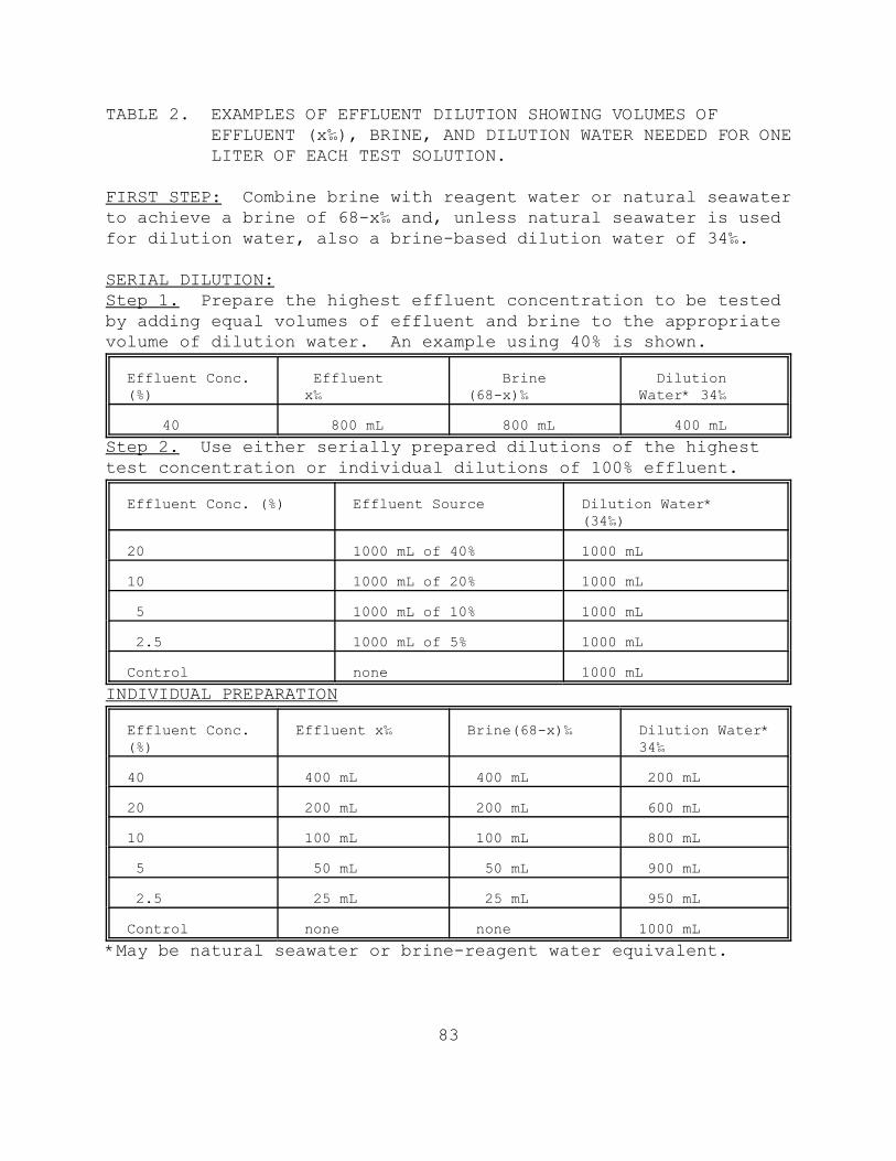
83

TABLE 2. EXAMPLES OF EFFLUENT DILUTION SHOWING VOLUMES OFEFFLUENT (x‰), BRINE, AND DILUTION WATER NEEDED FOR ONELITER OF EACH TEST SOLUTION.

FIRST STEP: Combine brine with reagent water or natural seawaterto achieve a brine of 68-x‰ and, unless natural seawater is usedfor dilution water, also a brine-based dilution water of 34‰.

SERIAL DILUTION:Step 1. Prepare the highest effluent concentration to be testedby adding equal volumes of effluent and brine to the appropriatevolume of dilution water. An example using 40% is shown.

Effluent Conc.(%)

Effluent x‰

Brine (68-x)‰

Dilution Water* 34‰

40 800 mL 800 mL 400 mLStep 2. Use either serially prepared dilutions of the highesttest concentration or individual dilutions of 100% effluent.

Effluent Conc. (%) Effluent Source Dilution Water* (34‰)

20 1000 mL of 40% 1000 mL

10 1000 mL of 20% 1000 mL

5 1000 mL of 10% 1000 mL

2.5 1000 mL of 5% 1000 mL

Control none 1000 mLINDIVIDUAL PREPARATION

Effluent Conc.(%)

Effluent x‰ Brine(68-x)‰ Dilution Water*34‰

40 400 mL 400 mL 200 mL

20 200 mL 200 mL 600 mL

10 100 mL 100 mL 800 mL

5 50 mL 50 mL 900 mL

2.5 25 mL 25 mL 950 mL

Control none none 1000 mL*May be natural seawater or brine-reagent water equivalent.

84

1-liter volumetric flask. Then, assuming an effluent salinity of2‰ and a brine salinity of 66‰, add 400 mL of brine (see equationabove and Table 2) and top off the flask with dilution water.Stopper the flask and shake well. Pour into a (100-250 mL)beaker and stir. Distribute equal volumes into the replicatetest chambers. The remaining test solution can be used forchemistry.

11.6.24.10 Brine Controls

11.6.24.10.1 Use brine controls in all tests where brine isused. Brine controls contain the same volume of brine as doesthe highest effluent concentration using brine, plus the volumeof reagent water needed to reproduce the hyposalinity of theeffluent in the highest concentration, plus dilution water. Calculate the amount of reagent water to add to brine controls byrearranging the above equation, (See SubSection, 11.6.24.8.3)setting SE = 0, and solving for VE.

VE = VB x (SB - 34)/(34 - SE)

11.6.25 BRINE SHRIMP, ARTEMIA SP., NAUPLII -- for feedingcultures and test organisms.

11.6.25.1 Newly hatched Artemia sp. nauplii are used for foodfor the test organisms. Although there are many commercialsources of brine shrimp cysts, the Brazilian or Colombian strainsare preferred because the supplies examined have had lowconcentrations of chemical residues and produce nauplii ofsuitably small size. (One source that has been found to beacceptable is Aquarium Products, 180L Penrod Ct., Glen Burnie,Maryland 21061). For commercial sources of brine shrimp,Artemia, cysts, see Table 2 of Section 5, Facilities, Equipment,and Supplies); and Section 4, Quality Assurance.

11.6.25.2 Each new batch of Artemia cysts must be evaluated forsize (Vanhaecke and Sorgeloos, 1980, and Vanhaecke et al., 1980)and nutritional suitability (Leger, et al., 1985, Leger, et al.,1986) against known suitable reference cysts by performing aside-by-side larval growth test using the "new" and "reference"cysts. The "reference" cysts used in the suitability test may bea previously tested and acceptable batch of cysts, or may beobtained from the Quality Assurance Research Division, EMSL,

85

Cincinnati, OH 45268, 513-569-7325. A sample of newly-hatchedArtemia nauplii from each new batch of cysts should be chemicallyanalyzed. The Artemia cysts should not be used if theconcentration of total organochlorine pesticides 0.15 ug/g wetweight or that the total concentration of organochlorinepesticides plus PCBs exceeds 0.30 µg/g wet weight (For analyticalmethods see USEPA, 1982).

11.6.25.3 Artemia nauplii are obtained as follows:

1. Add 1 L of seawater, or an aqueous unionized salt(NaCl) solution prepared with 35 g salt or artificialsea salts per liter, to a 2-L separatory funnel, orequivalent.

2. Add 10 mL Artemia cysts to the separatory funnel andaerate for 24 h at 27EC. Hatching time varies withincubation temperature and the geographic strain ofArtemia used (see USEPA, 1985a; USEPA, 1993a; ASTM,1993).

3. After 24 h, cut off the air supply in the separatoryfunnel. Artemia nauplii are phototactic, and willconcentrate at the bottom of the funnel if it iscovered for 5-10 minutes with a dark cloth or papertowel. To prevent mortality, do not leave theconcentrated nauplii at the bottom of the funnel morethan 10 min without aeration.

4. Drain the nauplii into a funnel fitted with a #150 µmNITEX® or stainless steel screen, and rinse withseawater or equivalent before use.

11.6.25.4 Testing Artemia nauplii as food for toxicity testorganisms.

11.6.25.4.1 The primary criteria for acceptability of each newsupply of brine shrimp cysts is adequate survival, and growth ofthe larvae. The larvae used to evaluate the acceptability of thebrine shrimp nauplii must be the same geographical origin andstage of development (9 to 15 days old) as those used routinelyin the toxicity tests. Two 7-day chronic tests are performedside-by-side, each consisting of five replicate test vesselscontaining five larvae (25 organisms per test, total of 50organisms). The juveniles in one set of test chambers is fed

86

reference (acceptable) nauplii and the other set is fed naupliifrom the "new" source of Artemia cysts.

11.6.25.4.2 The feeding rate and frequency, test vessels, volumeof control water, duration of the tests, and age of the Artemianauplii at the start of the test, should be the same as used forthe routine toxicity tests.

11.6.25.4.3 Results of the brine shrimp, Artemia, naupliinutrition assay, where there are only two treatments, can beevaluated statistically by use of a t test. The "new" food isacceptable if there are no statistically significant differencesin the survival or growth of the mysids fed the two sources ofnauplii.

11.6.26 TEST ORGANISMS

11.6.26.1 The test organisms for test method are larvae of thetopsmelt, Atherinops affinis. Topsmelt occur from the Gulf ofCalifornia to Vancouver Island, British Columbia (Miller and Lea,1972). It is often among the most abundant fish species incentral and southern California estuaries (Allen and Horn, 1975;Horn, 1979; Allen, 1982). Topsmelt reproduce from May throughAugust, depositing eggs on benthic algae in the upper ends ofestuaries and bays (Croaker, 1934; Fronk, 1969). Off-seasonspawning of Atherinops affinis has been successful in alaboratory-held population (Anderson et al., 1994). Theirembryonic development is similar to that of other atherinids usedwidely in toxicity testing (eg, Menidia species, Borthwick etal.,1985; Middaugh et al., 1987; Middaugh and Shenker, 1988), andmethods to assess sublethal effects with these species haveproven to be adaptable for topsmelt (Anderson et al., 1991,Middaugh and Anderson, 1993, McNulty et al., 1994).

11.6.26.2 Species Identification

11.6.26.2.1 Topsmelt often co-occur with jacksmelt, Atherinopsiscaliforniensis. The two species can be distinguished based onseveral key characteristics. Jacksmelt have 10-12 scales betweentheir two dorsal fins; topsmelt have 5-8 scales between the twofins. Jacksmelt teeth are arranged in several bands on each jawand the teeth are not forked; topsmelt teeth are arranged in oneband and the teeth are forked. In jacksmelt, the insertion of

87

the first dorsal fin occurs well in advance of the origin of theanal fin. In topsmelt, the origin of the anal fin is under theinsertion of the first dorsal fin. Consult Miller and Lea (1972)for a guide to the taxonomy of these two fishes.

11.6.26.3 Obtaining Broodstock

11.6.26.3.1 In California, adult topsmelt can be seined fromsandy beaches in sloughs and estuaries from April through August. The size of the seine used depends on the number of peopledeploying it and the habitat being sampled. Larger seines can beused in open sandy areas, smaller seines are used in smallerareas with rocky outcroppings. Five or six people are anadequate number to set and haul a 100-ft beach seine. The seineis set on an ebbing tide using a small motor skiff with oneperson driving and a second deploying the net from the bow. Thenet is set parallel to shore then hauled in evenly from thewings. The net mesh diameter should be small enough to preventthe fish from damaging themselves; a one-centimeter diameter meshin the middle panel and one-and-a-half-centimeter diameter meshin the wing panel is adequate. As the net is pulled onto theshore, the adult topsmelt are sorted into five-liter plasticbuckets, then immediately transferred to 100-liter transporttanks.

11.6.26.3.2 State collection permits are usually required forcollection of topsmelt. Collection is prohibited or restrictedin some areas. Collection of topsmelt is regulated by Californialaw. Collectors must obtain a scientific collector's permit fromthe California Department of Fish and Game and observe anyregulations regarding collection, transfer, and maintenance offish broodstock.

11.6.26.3.3 Various containers can be used to transport fish;100-liter covered plastic trash cans have been used successfullyto transport topsmelt. New plastic containers should be leachedin seawater for 96 hours prior to transporting fish. Eachcontainer can maintain approximately 20 adult fish for six toeight hours if adequate aeration is provided. Use compressedoxygen or air to supply aeration to the tanks during transport.

11.6.26.4 Broodstock Culture and Handling

88

11.6.26.4.1 Once in the laboratory the fish should be treatedfor 2 days with a general antibiotic in a separate tank (eg.,Prefuran® as per label instructions), then divided among 1000-liter holding tanks. No more than 30 adult fish should be placedin each tank. Tank temperature should be maintained at 18ECusing a 1500-watt immersion heater. To conserve heated seawater,the seawater in the tanks can be recirculated using the systemsimilar to that described by Middaugh and Hemmer (1984). A one-thirtieth (1/30)-hp electric pump is used to circulate water (10liters/minute) from the tanks through vertical, biologicallyactivated nylon filter elements located in a separate reservoir,then back into the tanks. Fresh seawater should be constantlyprovided to the system at 0.5 liters/minute to supplement therecirculated seawater. The tanks are insulated with one inchthick closed cell foam to conserve heat. Dissolved oxygen levelsshould be maintained at greater than 6.0 mg/liter using aeration. Salinity should be checked periodically using a refractometeraccurate to the nearest 0.5‰; tank salinity should be 34 ± 2‰.

11.6.26.4.2 Adult topsmelt in each tank are fed twice daily (at0900 and 1500 hrs) approximately 0.3g of Tetramin™ flake food. Supplemental feedings of krill or chopped squid are recommended.Tanks are siphoned clean once weekly.

11.6.26.4.3 Dyeless yarn spawning substrates are attached to thesurface of plastic grids cut from light diffuser panel (7 cm x10 cm x 1 cm) and weighted to the bottom of each tank. Substrates are checked daily for the presence of eggs.

11.6.26.4.4 Spawning is induced by a combination of threeenvironmental cues: lighting, 'tidal' cycle, and temperature. The photoperiod is 14 hours of light followed by 10 hours ofdarkness (14L:10D) with lights on at 0600 and off at 2000 hours. Use two cool white 40-watt fluorescent lamps suspended 1.25 meters above the surface of each tank to provide illumination. Light levels at the surface of the tanks should be 12 to 21µE/m2/s.

11.6.26.4.5 A 'tidal signal' of reduced current velocity isproduced once daily in each tank, from 2400 to 0200 hrs, byturning off the circulating pump (Middaugh and Hemmer, 1984).A 1500-watt immersion heater is used to maintain constanttemperature at 18EC and to provide temperature spikes. For

89

spiking, the temperature is raised from 18EC to 21EC over a 12 hperiod, then allowed to return to 18EC overnight. The temperatureshould be checked to the nearest 0.1EC at 1 to 4 hour intervalson days when the temperature spikes are introduced. It is commonfor the fish to appear stressed during the temperature increaseand one or two fish may die. If significant mortality begins tooccur, the temperature should be lowered immediately. Significant egg production usually begins within five days of thetemperature spike (Middaugh, et al., 1992).

11.6.26.5 Culture Materials

11.6.26.5.1 See Section 5, Facilities and Equipment, for adiscussion of suitable materials to be used in laboratory cultureof topsmelt. Be sure all new materials are properly leached inseawater before use. After use, all culture materials should bewashed in soap and water, then rinsed with seawater before re-use.

11.6.26.6 Test Organisms

11.6.26.6.1. Newly fertilized embryos should be placed in screentubes set in aquaria and equipped with gently flowing seawater at20 ± 1EC. The embryos can be left attached to the spawningsubstrates but care should be taken to ensure the substrates arerelatively clean and free of food; strands of embryos should notoverlap each other on the substrates, and gentle aeration must beprovided. Beginning about day 9, check the screen tubes dailyfor the presence of larvae. Isolate newly-hatched larvae into aseparate screen-tube at 21EC by slow siphoning. Provide larvaewith newly-hatched Artemia nauplii (in excess) at 24-h post-hatch; supply gently flowing seawater, and aeration. Larvaeaged 9 to 15 days are used in toxicity tests (McNulty et al.,1994). For information regarding topsmelt larva suppliers callthe Marine Pollution Studies Laboratory (408) 624-0947.

11.6.26.6.2 Larvae can be transported in 1-liter ziplock plasticbags (double-bagged). No more than approximately 100 larvaeshould be transported in any one bag; do not include food. Theseawater in the bags should be aerated with pure oxygen for 30seconds prior to introduction of the larvae. The bag should bepacked in an ice chest with one or two blue ice blocks (insulatedby newspaper) for transport. The temperature during transport

90

should be held between 15 and 18EC. Larvae should be shipped viaair-express overnight couriers.

11.6.26.6.3 Topsmelt larvae can tolerate a relatively wide rangeof salinities (5 to $35‰) if adequate acclimation is provided(Anderson, et al., In Press). In situations where the testsalinity is significantly lower than the salinity at which thelarvae were cultured, it may be necessary to acclimate the larvaeto the test salinity.

11.7 EFFLUENTS AND RECEIVING WATER COLLECTION, PRESERVATION, AND STORAGE

11.7.1 See Section 8, Effluent and Receiving Water Sampling,Sample Handling, and Sample Preparation for Toxicity Tests.

11.8 CALIBRATION AND STANDARDIZATION

11.8.1 See Section 4, Quality Assurance

11.9 QUALITY CONTROL

11.9.1 See Section 4, Quality Assurance

11.10 TEST PROCEDURES

11.10.1 TEST DESIGN

11.10.1.1 The test consists of at least five effluentconcentrations plus a dilution water control. Tests that usebrine to adjust salinity must also contain five replicates of abrine control.

11.10.1.2 Effluent concentrations are expressed as percenteffluent.

11.10.2 TEST SOLUTIONS

11.10.2.1 Receiving waters

11.10.2.1.1 The sampling point is determined by the objectivesof the test. At estuarine and marine sites, samples are usuallycollected at mid-depth. Receiving water toxicity is determined

91

with samples used directly as collected or with samples passedthrough a 60 µm NITEX® filter and compared without dilution,against a control. Using five replicate chambers per test, eachcontaining 200 mL would require approximately 1 L of sample pertest per day.

11.10.2.2 Effluents

11.10.2.2.1 The selection of the effluent test concentrationsshould be based on the objectives of the study. A dilutionfactor of at least 0.5 is commonly used. A dilution factor of0.5 provides hypothesis test discrimination of ± 100%, andtesting of a 16 fold range of concentrations. Hypothesis testdiscrimination shows little improvement as dilution factors areincreased beyond 0.5 and declines rapidly if smaller dilutionfactors are used. USEPA recommends that one of the five effluenttreatments must be a concentration of effluent mixed withdilution water which corresponds to the permittee's instreamwaste concentration (IWC). At least two of the effluenttreatments must be of lesser effluent concentration than the IWC,with one being at least one-half the concentration of the IWC. If 100‰ HSB is used as a diluent, the maximum concentration ofeffluent that can be tested will be 66% at 34‰ salinity.

11.10.2.2.2 If the effluent is known or suspected to be highlytoxic, a lower range of effluent concentrations should be used(such as 25%, 12.5%, 6.25%, 3.12% and 1.56%).

11.10.2.2.3 The volume in each test chamber is 200 mL.

11.10.2.2.4 Effluent dilutions should be prepared for allreplicates in each treatment in one container to minimizevariability among the replicates. Dispense into the appropriateeffluent test chambers.

11.10.2.3 Dilution Water

11.10.2.3.1 Dilution water should be uncontaminated 1-µm-filtered natural seawater or hypersaline brine prepared fromuncontaminated natural seawater plus reagent water (see Section7, Dilution Water). Natural seawater may be uncontaminatedreceiving water. This water is used in all dilution steps and asthe control water.

92

11.10.2.4 Reference Toxicant Test

11.10.2.4.1 Reference toxicant tests should be conducted asdescribed in Quality Assurance (see Section 4.7).

11.10.2.4.2 The preferred reference toxicant for topsmelt iscopper chloride (CuCl2N2H2O). Reference toxicant tests providean indication of the sensitivity of the test organisms and thesuitability of the testing laboratory (see Section 4 QualityAssurance). Another toxicant may be specified by the appropriateregulatory agency. Prepare a 10,000 µg/L copper stock solutionby adding 0.0268 g of copper chloride (CuCl2N2H2O) to one literof reagent water in a polyethylene volumetric flask. Alternatively, certified standard solutions can be ordered fromcommercial companies.

11.10.2.4.3 Reference toxicant solutions should be fivereplicates each of 0 (control), 56, 100, 180, and 320 µg/L totalcopper. Prepare one liter of each concentration by adding 0,5.6, 10.0, 18.0, and 32.0 mL of stock solution, respectively, toone-liter volumetric flasks and fill with dilution water. Startwith control solutions and progress to the highest concentrationto minimize contamination.

11.10.2.4.4 If the effluent and reference toxicant tests are tobe run concurrently, then the tests must use embryos from thesame spawn. The tests must be handled in the same way and testsolutions delivered to the test chambers at the same time. Reference toxicant tests must be conducted at 34 ± 2‰.

11.10.3 START OF THE TEST

11.10.3.1 Prior to Beginning the Test

11.10.3.1.1 The test should begin as soon as possible, preferably within 24 h of sample collection. The maximum holdingtime following retrieval of the sample from the sampling deviceshould not exceed 36 h for off-site toxicity tests unlesspermission is granted by the permitting authority. In no caseshould the sample be used in a test more than 72 h after samplecollection (see Section, 8 Effluent and Receiving Water Sampling,Sample Handling, and Sample Preparation for Toxicity Test).

93

11.10.3.1.2 Just prior to test initiation (approximately 1 h),the temperature of a sufficient quantity of the sample to makethe test solutions should be adjusted to the test temperature (20± 1EC) and maintained at that temperature during the addition ofdilution water.

11.10.3.1.3 Increase the temperature of the water bath, room, orincubator to the required test temperature (20 ± 1EC).

11.10.3.1.4 Randomize the placement of test chambers in thetemperature-controlled water bath, room, or incubator at thebeginning of the test, using a position chart. Assign numbersfor the position of each test chamber using a random numbers orsimilar process (see Appendix A, for an example ofrandomization). Maintain the chambers in this configurationthroughout the test, using a position chart. Record thesenumbers on a separate data sheet together with the concentrationand replicate numbers to which they correspond. Identify thissheet with the date, test organism, test number, laboratory, andinvestigator's name, and safely store it away until after thelarvae have been examined at the end of the test.

11.10.3.1.5 Note: Loss of the randomization sheet wouldinvalidate the test by making it impossible to analyze the dataafterwards. Make a copy of the randomization sheet and storeseparately. Take care to follow the numbering system exactlywhile filling chambers with the test solutions.

11.10.3.1.6 Arrange the test chambers randomly in the water bathor controlled temperature room. Once chambers have been labeledrandomly, they can be arranged in numerical order forconvenience, since this will also ensure random placement oftreatments.

11.10.3.2 Randomized Placement of Larvae into Test Chambers

11.10.3.2.1 Larvae must be randomized before placing them intothe test chambers. Pool all of the test larvae into a 1-literbeaker by slow siphoning from the screen-tube. The larvae in thescreen-tube can be concentrated into the bottom by lifting thetube during siphoning. Using a fire-polished glass tube, placeone larva into as many plastic cups as there are test chambers(including reference toxicant chambers). These cups should

94

contain enough reference seawater to maintain water quality andtemperature during the transfer process (approx. 50 mL). Wheneach of the cups contains one larva, repeat the process, addingone larva at a time until each cup contains 5 animals.

11.10.3.2.2 Carefully pour or pipet off excess water in thecups, leaving less than 5 mL with the test larvae. If more than5 mLs of water are added to the test solution with the juveniles,report the amount on the data sheet. Carefully transfer thelarvae into the test chambers immediately after reducing thewater volume. Again, make note of any excess dilution of thetest solution. Because of the small volumes involved in thetransfer process, this is best accomplished in a constanttemperature room. Be sure that all water used in culture,transfer, and test solutions is within 1EC of the testtemperature.

11.10.3.2.3 Verify that all five animals are transferred bycounting the number in each chamber after transfer. This initialcount is important because larvae unaccounted for at the end ofthe test are assumed to be dead.

11.10.4 LIGHT, PHOTOPERIOD, SALINITY AND TEMPERATURE

11.10.4.1 The light quality and intensity should be at ambientlaboratory conditions are generally adequate. Light intensityshould be 10-20 µE/m2/s, or 50 to 100 foot candles (ft-c), with a16 h light and 8 h dark cycle.

11.10.4.2 The water temperature in the test chambers should bemaintained at 20 ± 1EC. If a water bath is used to maintain thetest temperature, the water depth surrounding the test cupsshould be as deep as possible without floating the chambers.

15.10.4.3 The test salinity should be in the range of 5 to 34‰,and the salinity should not vary by more than ± 2‰ among thechambers on a given day. The salinity should vary by no morethan ±2‰ among the chambers on a given day. If effluent andreceiving water tests are conducted concurrently, the salinitiesof these tests should be similar.

15.10.4.4 Rooms or incubators with high volume ventilationshould be used with caution because the volatilization of the

95

test solutions and evaporation of dilution water may cause widefluctuations in salinity. Covering the test chambers with cleanpolyethylene plastic may help prevent volatilization andevaporation of the test solutions.

11.10.5 DISSOLVED OXYGEN (DO) CONCENTRATION

11.10.5.1 Aeration may affect the toxicity of effluent andshould be used only as a last resort to maintain a satisfactoryDO. The DO concentration should be measured on new solutions atthe start of the test (Day 0). The DO should not fall below 4.0mg/L (see Section 8, Effluent and Receiving Water Sampling,Sample Handling, and Sample Preparation for Toxicity Tests). Ifit is necessary to aerate, all treatments and the control shouldbe aerated. The aeration rate should not exceed that necessaryto maintain a minimum acceptable DO and under no circumstancesshould it exceed 100 bubbles/minute, using a pipet with a 1-2 mmorifice, such as a 1 mL KIMAX® serological pipet No. 37033, orequivalent. Care should be taken to ensure that turbulenceresulting from aeration does not cause undue stress to the fish.

11.10.6 FEEDING

11.10.6.1 Artemia nauplii are prepared as described below.

11.10.6.2 The test larvae are fed newly-hatched (less than 24-h-old) Artemia nauplii once a day from Day 0 through Day 6; larvaeare not fed on Day 7. Equal amounts of Artemia nauplii must befed to each replicate test chamber to minimize the variability oflarval weight. Add 40 newly hatched Artemia nauplii per larvatwice daily: once in the morning and once in the afternoon. Thedensity of Artemia may be determined by pipetting a known volumeof nauplii onto a piece of filter paper and counting the numberusing a dissecting microscope. Feeding excessive amounts ofArtemia nauplii will result in a depletion in DO to below anacceptable level. Siphon as much of the uneaten Artemia naupliias possible from each chamber daily to ensure that the larvaeprincipally eat newly hatched nauplii.

11.10.7 DAILY CLEANING OF TEST CHAMBERS

11.10.7.1 Before the daily renewal of test solutions, uneatenand dead brine shrimp, dead larvae, and other debris are removed

96

from the bottom of the test chambers with a siphon hose. Becauseof their small size during the first few days of the test, larvaeare easily drawn into a siphon tube when cleaning the testchambers. By placing the test chambers on a light box,inadvertent removal of larvae can be greatly reduced because theycan be more easily seen. If the water siphoned from the testchambers is collected in a white plastic tray, the live larvaecaught up in the siphon can be retrieved, and returned by pipetteto the appropriate test chamber and noted on the data sheet.

11.10.8 OBSERVATIONS DURING THE TEST

11.10.8.1 Routine Chemical and Physical Observations

11.10.8.1.1 DO is measured at the beginning of the exposureperiod in one test chamber at each test concentration and in thecontrol.

11.10.8.1.2 Temperature, pH, and salinity are measured at thebeginning of the exposure period in one test chamber at eachconcentration and in the control. Temperature should also bemonitored continuously or observed and recorded daily for atleast two locations in the environmental control system or thesamples. Temperature should be measured in a sufficient numberof test chambers at the end of the test to determine temperaturevariation in the environmental chamber.

11.10.8.1.3 Record all the measurements on the data sheet.

11.10.8.2 Routine Biological Observations

11.10.8.2.1 The number of live larvae in each test chamber arerecorded daily and the dead larvae are discarded. These dataprovide daily mortality rates which may be used to calculate 24,48, and 96-h LC50s.

11.10.8.2.2 Protect the larvae from unnecessary disturbancesduring the test by carrying out the daily test observations,solution renewals, and removal of dead larvae, carefully. Makesure the larvae remain immersed at all times during theperformance of the above operations.

97

11.10.9 TEST SOLUTION RENEWAL

11.10.9.1 The test solutions are renewed daily using freshlyprepared solutions, immediately after cleaning the test chambers. The old solution is carefully siphoned out, leaving enough waterso that all of the larvae can still swim freely (approximately 50mL). Siphon from the bottom of the test chambers so that deadArtemia nauplii are removed with the old test solution. It isconvenient to siphon old solutions into a small (~500 mL)container in order to ensure that no larvae have beeninadvertently removed during solution renewals. If a larva issiphoned, return it to the test chamber and note it on the datasheet.

11.10.9.2 New solution is siphoned into the test chambers usinga U-shaped glass tube attached to plastic tubing to minimizedisturbance to the larvae.

11.10.9.3 The effluent or receiving water used in the test isstored in an incubator or refrigerator at 4EC. Plasticcontainers such as 8-20 L cubitainers have proven suitable foreffluent collection and storage. For on-site toxicity studies nomore than 24 h should elapse between collection of the effluentand use in a toxicity test (see Section 8, Effluent and ReceivingWater Sampling, Sample Handling, and Sample Preparation forToxicity Tests).

11.10.9.4 Approximately 1 h before test initiation, a sufficientquantity of effluent or receiving water sample is warmed to 20 ±1EC to prepare the test solutions. A sufficient quantity ofeffluent should be warmed to make daily test solutions.

11.10.10 TERMINATION OF THE TEST

11.10.10.1 Ending the Test

11.10.10.1.1 Record the time the test is terminated.

11.10.10.1.2 Temperature, pH, dissolved oxygen, and salinity aremeasured at the end of the exposure period in one test chamber ateach concentration and in the control.

11.10.10.2 Sample Preservation

98

11.10.10.2.1 The surviving larvae in each test chamber(replicate) are counted, and immediately prepared as a group fordry weight determination, or are preserved in 4% formalin then70% ethanol. Preserved organisms are dried and weighed within 7d. For safety, formalin should be used under a hood. Note: Death is defined as lack of response to stimulus such as proddingwith a glass rod; dead larvae are generally opaque and curled.

11.10.10.3 Weighing

11.10.10.3.1 For immediate drying and weighing, siphon or pourlive larvae onto a 500 µm mesh screen in a large beaker to retainthe larvae and allow Artemia to be rinsed away. Rinse the larvaewith reagent water to remove salts that might contribute to thedry weight. Sacrifice the larvae in an ice bath of reagentwater.

11.10.10.3.2 Small aluminum weighing pans can be used to dry andweigh larvae. An appropriate number of aluminum weigh pans (oneper replicate) are marked for identification and weighed to 0.01mg, and the weights are recorded on the data sheets.

11.10.10.3.3 Immediately prior to drying, the preserved larvaeare in reagent water. The rinsed larvae from each test chamberare transferred, using forceps, to a tared weighing pans anddried at 60EC for 24 h, or at 105EC for a minimum of 6 h. Immediately upon removal from the drying oven, the weighing pansare placed in a desiccator to cool and to prevent the adsorptionof moisture from the air until weighed. Weigh all weighing panscontaining the dried larvae to 0.01 mg, subtract the tare weightto determine dry weight of larvae in each replicate. Record theweights.

11.10.10.4 Endpoints

11.10.10.4.1 Divide the dry weight by the number of originallarvae (5) per replicate to determine the average dry weight, andrecord on the data sheets. For the controls, also calculate themean weight per surviving fish in the test chamber to evaluate ifweights met test acceptability criteria (see Subsection 11.11). Complete the summary data sheet after calculating the averagemeasurements and statistically analyzing the dry weights and

99

percent survival for the entire test. Average weights should beexpressed to the nearest 0.01 mg.

11.11 SUMMARY OF TEST CONDITIONS AND TEST ACCEPTABILITY CRITERIA

11.11.1 A summary of test conditions and test acceptabilitycriteria is listed in Table 3.

TABLE 3. SUMMARY OF TEST CONDITIONS AND TEST ACCEPTABILITYCRITERIA FOR THE TOPSMELT, ATHERINOPS AFFINIS, LARVALSURVIVAL AND GROWTH TEST WITH EFFLUENTS AND RECEIVINGWATERS

1. Test type: Static-renewal

2. Salinity: 5 to 34‰ (± 2‰ of the selectedtest salinity)

3. Temperature: 20 ± 1EC

4. Light quality: Ambient laboratory illumination

5. Light intensity: 10-20 µE/m2/s (Ambientlaboratory levels)

6. Photoperiod: 16 h light, 8 h darkness

7. Test chamber size: 600 mL

8. Test solution volume: 200 mL/replicate

9. Renewal of testsolutions:

Daily

10. Age of test organisms: 9-15 days post-hatch

11. No. larvae per testchamber:

5

12. No. replicate chambersper concentration:

5

13. Source of food: Newly hatched Artemia nauplii

14. Feeding regime: Feed 40 nauplii per larvaetwice daily (morning and night)

100

15. Cleaning: Siphon daily, immediatelybefore test solution renewaland feeding

16. Aeration: None, unless DO concentrationfalls below 4.0 mg/L, thenaerate all chambers. Rateshould be less than 100bubbles/min.

17. Dilution water: Uncontaminated 1-µm-filterednatural seawater or hypersalinebrine prepared from naturalseawater

18. Test concentrations: Effluent: Minimum of 5 and acontrolReceiving waters: 100%receiving water and a control

19. Dilution factor: Effluents: $0.5Receiving waters: None, or $0.5

20. Test duration: 7 days

21. Endpoints: Survival and growth (weight)

22. Test acceptabilitycriteria:

$80% survival in controls, 0.85mg average weight of controllarvae (9 day old), LC50 withcopper must be #205 µg/L, <25%MSD for survival and <50% MSDfor growth

101

23. Sampling requirement: For on-site tests, samplescollected daily, and usedwithin 24 h of the time theyare removed from the samplingdevice. For off-site tests, aminimum of three samples arecollected on days one, three,and five with a maximum holdingtime of 36 h before first use(see Section 8, Effluent andReceiving Water Sampling,Sample Handling, and SamplePreparation for Toxicity Tests)

24. Sample volumerequired:

2 L per day

11.12 ACCEPTABILITY OF TEST RESULTS

11.12.1 Tests results are acceptable only if all the followingrequirements are met:

(1) The mean survival of larvae must be at least 80% in thecontrols.

(2) If the test starts with 9 day old larvae, the meanweight per larva must exceed 0.85 mg in the referenceand brine controls; the mean weight of preserved larvaemust exceed 0.72 mg.

(3) The LC50 for survival must be within two standarddeviations of the control chart mean for thelaboratory. The LC50 for survival with copper must be<205 µg/L.

(4) The minimum significant difference (%MSD) of <25%relative to the control for survival for the referencetoxicant test. The (%MSD) of <50% relative to thecontrol for growth for the reference toxicant test.

11.13 DATA ANALYSIS

102

11.13.1 GENERAL

11.13.1.1 Tabulate and summarize the data. A sample set ofsurvival and growth response data is listed in Table 4.

11.13.1.2 The endpoints of toxicity tests using the topsmeltlarvae are based on the adverse effects on survival and growth. The LC50 and the IC25 are calculated using point estimationtechniques (see Section 9, Chronic Toxicity Test Endpoints andData Analysis). LOEC and NOEC values, for survival and growth,are obtained using a hypothesis testing approach such asDunnett's Procedure (Dunnett, 1955) or Steel's Many-one Rank Test(Steel, 1959; Miller, 1981)(see Section 9). Separate analysesare performed for the estimation of the LOEC and NOEC endpointsand for the estimation of the LC50 and IC25. Concentrations atwhich there is no survival in any of the test chambers areexcluded from the statistical analysis of the NOEC and LOEC forsurvival and growth, but included in the estimation of the LC50and IC25. See the Appendices for examples of the manualcomputations and examples of data input and program output.

11.13.1.3 The statistical tests described here must be used witha knowledge of the assumptions upon which the tests arecontingent. Tests for normality and homogeneity of variance areincluded in Appendix B. The assistance of a statistician isrecommended for analysts who are not proficient in statistics.

11.13.2 EXAMPLE OF ANALYSIS OF TOPSMELT, ATHERINOPS AFFINISSURVIVAL DATA

11.13.2.1 Formal statistical analysis of the survival data isoutlined in Figures 1 and 2. The response used in the analysis isthe proportion of animals surviving in each test or controlchamber. Separate analyses are performed for the estimation ofthe NOEC and LOEC endpoints and for the estimation of the LC50endpoint. Concentrations at which there is no survival in any ofthe test chambers are excluded from statistical analysis of theNOEC and LOEC, but included in the estimation of the IC, EC, andLC endpoints.

11.13.2.2 For the case of equal numbers of replicates across allconcentrations and the control, the evaluation of the NOEC andLOEC endpoints is made via a parametric test, Dunnett's

103

Procedure, or a nonparametric test, Steel's Many-one Rank Test,on the arc sine square root transformed data. Underlyingassumptions of Dunnett's Procedure, normality and homogeneity ofvariance, are formally tested. The test for normality is theShapiro-Wilk's Test, and Bartlett's Test is used to test forhomogeneity of variance. If either of these tests fails, thenonparametric test, Steel's Many-one Rank Test, is used todetermine the NOEC and LOEC endpoints. If the assumptions ofDunnett's Procedure are met, the endpoints are estimated by theparametric procedure.

11.13.2.3 If unequal numbers of replicates occur among theconcentration levels tested, there are parametric andnonparametric alternative analyses. The parametric analysis is at test with the Bonferroni adjustment (see Appendix D). TheWilcoxon Rank Sum Test with the Bonferroni adjustment is thenonparametric alternative.

11.13.2.4 Probit Analysis (Finney, 1971; see Appendix H) is usedto estimate the concentration that causes a specified percentdecrease in survival from the control. In this analysis, thetotal mortality data from all test replicates at a givenconcentration are combined. If the data do not fit the ProbitAnalysis, the Spearman-Karber Method, the Trimmed Spearman-KarberMethod, or the Graphical Method may be used to estimate the LC50(see Appendices H-K).

11.13.2.5 Example of Analysis of Survival Data

11.13.2.5.1 This example uses the survival data from theTopsmelt Larval Survival and Growth Test. The proportionsurviving in each replicate must first be transformed by the arcsine square root transformation procedure described in Appendix . The raw and transformed data, means and variances of thetransformed observations at each copper concentration and controlare listed in Table 5. A plot of the survival proportions isprovided in Figure 5. Since there was 100% mortality in all fivereplicates for the 100 µg/L and 180 µg/L concentrations, they arenot included in the statistical analysis and are consideredqualitative mortality effects.

104

TABLE 4. SUMMARY OF SURVIVAL AND GROWTH DATA FOR TOPSMELT,ATHERINOPS AFFINIS, LARVAE EXPOSED TO COPPER FORSEVEN DAYS1

Copper Mean Conc. Replicate Survival Proportions Proportion (µg/L) A B C D E Survival

0.0 1.0 0.8 1.0 1.0 1.0 0.96 32.0 1.0 1.0 1.0 1.0 1.0 1.00 56.0 0.0 0.6 0.2 1.0 0.6 0.48 100.0 0.0 0.0 0.0 0.0 0.0 0.00 180.0 0.0 0.0 0.0 0.0 0.0 0.00 Conc. Replicate Average Dry Weights (mg) Mean Dry (µg/L) A B C D E Wgt (mg) 0.0 0.00134 0.00153 0.00134 0.00146 0.00144 0.00142 32.0 0.00146 0.00142 0.00150 0.00138 0.00128 0.00141 56.0 -- 0.00147 0.00170 0.00124 0.00130 0.00114 100.0 -- -- -- -- -- -- 180.0 -- -- -- -- -- --

1Five replicates of 5 larvae each.

105

Figure 1. Flowchart for statistical analysis of the topsmelt,Atherinis affinis, larval survival data by hypothesis testing.

106

Figure 2. Flowchart for statistical analysis of the topsmelt, Atherinis affinis, larval survival data by point estimation.

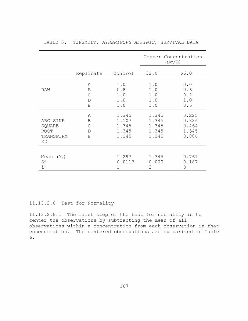
107

TABLE 5. TOPSMELT, ATHERINOPS AFFINIS, SURVIVAL DATA

Replicate Control

Copper Concentration(µg/L)

32.0 56.0

RAWABCDE

1.00.81.01.01.0

1.01.01.01.01.0

0.00.60.21.00.6

ARC SINESQUAREROOTTRANSFORMED

ABCDE

1.3451.1071.3451.3451.345

1.3451.3451.3451.3451.345

0.2250.8860.4641.3450.886

_Mean (Yi)S2ii

1.2970.01131

1.3450.0002

0.7610.1873

11.13.2.6 Test for Normality

11.13.2.6.1 The first step of the test for normality is tocenter the observations by subtracting the mean of allobservations within a concentration from each observation in thatconcentration. The centered observations are summarized in Table6.

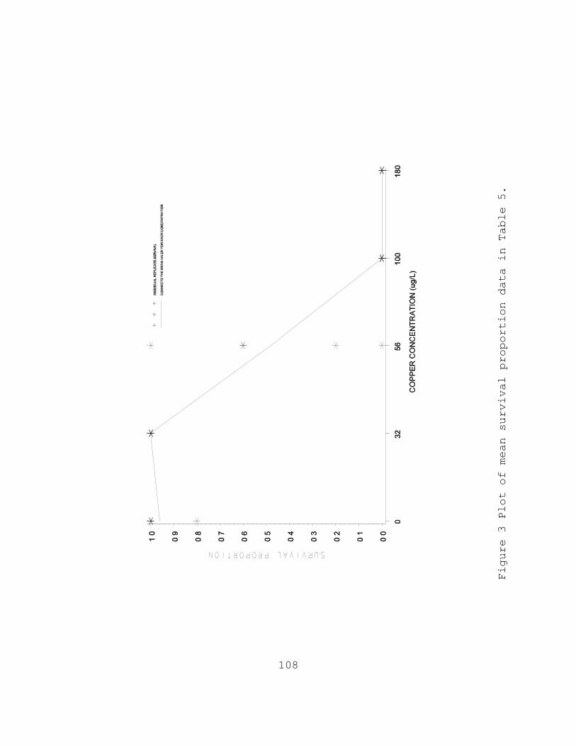
108

Figure 3 Plo

t of

mea

n su

rviv

al p

ropo

rtio

n da

ta in

Tabl

e 5.

109

TABLE 6. CENTERED OBSERVATIONS FOR SHAPIRO-WILK'S EXAMPLE

Replicate Control

Copper Concentration(µg/L)

32.0 56.0

ABCDE

0.048-0.190 0.048 0.048 0.048

0.000 0.000 0.000 0.000 0.000

-0.536 0.125-0.297 0.584 0.125

D ' 'ni'1(Xi&X)

2

11.13.2.6.2 Calculate the denominator, D, of thestatistic:

Where: Xi = the ith centered observation X& = the overall mean of the centered observations n = the total number of centered observations

11.13.2.6.3 For this set of data,

n = 15 X& = 1 (0.003) = 0.000 15

D = 0.793

11.13.2.6.4 Order the centered observations from smallest tolargest

X(1) # X(2) # ... # X(n)

110

TABLE 7. ORDERED CENTERED OBSERVATIONS FOR THE SHAPIRO-WILK'S EXAMPLE

i X(i) i X(i)

1 -0.536 9 0.048 2 -0.297 10 0.048 3 -0.190 11 0.048 4 0.000 12 0.048 5 0.000 13 0.125 6 0.000 14 0.125 7 0.000 15 0.584 8 0.000

W '1D[ 'ki'1ai(X

(n&i%1)&X (i))]2

W '1

0.793(0.817)2 ' 0.842

where X(i) denotes the ith ordered observation. The orderedobservations for this example are listed in Table 7.

11.13.2.6.5 From Table 4, Appendix B, for the number ofobservations, n, obtain the coefficients a1, a2, ... ak where k isn/2 if n is even and (n-1)/2 if n is odd. For the data in thisexample, n = 15 and k = 7. The ai values are listed in Table 8.

11.13.2.6.6 Compute the test statistic, W, as follows:

The differences X(n-i+1) - X(i) are listed in Table 7. For the data in this example,

11.13.2.6.7 The decision rule for this test is to compare W ascalculated in Subsection 11.13.2.6.6 to a critical value found inTable 6, Appendix B. If the computed W is less than the criticalvalue, conclude that the data are not normally distributed. Forthe data in this example, the critical value at a significance

111

TABLE 8. COEFFICIENTS AND DIFFERENCES FOR SHAPIRO-WILK'S EXAMPLE

i ai X(n-i+1) - X(i) 1 0.5150 1.120 X(15) - X(1) 2 0.3306 0.422 X(14) - X(2) 3 0.2495 0.315 X(13) - X(3) 4 0.1878 0.048 X(12) - X(4) 5 0.1353 0.048 X(11) - X(5) 6 0.0880 0.048 X(10) - X(6) 7 0.0433 0.048 X(9) - X(7)

level of 0.01 and n = 15 observations is 0.835. Since W = 0.842is greater than the critical value, conclude that the data arenormally distributed.

11.13.2.6.8 Since the variance of the lowest copperconcentration group is zero, Bartlett's test statistic can not becalculated. Therefore, the survival data variances areconsidered to be heterogeneous.

11.13.2.6.9 Since the data do not meet the assumption ofhomogeneity of variance, Steel's Many-one Rank Test will be used

to analyze the survival data.

11.13.2.7 Steel's Many-one Rank Test 11.13.2.7.1 For each control and concentration combination,combine the data and arrange the observations in order of sizefrom smallest to largest. Assign the ranks (1, 2, ..., 10) tothe ordered observations with a rank of 1 assigned to thesmallest observation, rank of 2 assigned to the next largerobservation, etc. If ties occur when ranking, assign the averagerank to each tied observation.

112

11.13.2.7.2 An example of assigning ranks to the combined datafor the control and 32.0 µg/L copper concentration is given inTable 9. This ranking procedure is repeated for each control/concentration combination. The complete set of rankingsis summarized in Table 10. The ranks are next summed for eachcopper concentration, as shown in Table 11.

11.13.2.7.3 For this example, determine if the survival in anyof the copper concentrations is significantly lower than thesurvival in the control. If this occurs, the rank sum at thatconcentration would be significantly lower than the rank sum ofthe control. Thus, compare the rank sums for the survival ateach of the various copper concentrations with some "minimum" orcritical rank sum, at or below which the survival would beconsidered significantly lower than the control. At asignificance level of 0.05, the minimum rank sum in a test withtwo concentrations (excluding the control) and five replicates is18 (see Table 5, Appendix E).

11.13.2.7.4 Since the rank sum for the 56.0 µg/L copperconcentration is equal to the critical value, the proportionsurviving in the 56.0 µg/L concentration is consideredsignificantly less than that in the control. Since the otherrank sum is not less than or equal to the critical value, it isnot considered to have a significantly lower proportion survivingthan the control. Hence, the NOEC and the LOEC are the 32.0 µg/Land 56.0 µg/L concentrations, respectively.

11.13.2.8 Calculation of the LC50

11.13.2.8.1 The data used for the calculation of the LC50 issummarized in Table 12. For estimating the LC50, the data forthe 100 µg/L and 180 µg/L copper concentrations with 100%mortality are included.

113

TABLE 9. ASSIGNING RANKS TO THE CONTROL AND 32.0 µg/LCOPPER CONCENTRATION FOR STEEL'S MANY-ONE RANKTEST

Rank Transformed Copper Proportion Concentration

Surviving (µg/L)

1 1.107 Control 6 1.345 32.0 6 1.345 32.0 6 1.345 32.0 6 1.345 32.0 6 1.345 32.0 6 1.345 Control 6 1.345 Control 6 1.345 Control 6 1.345 Control

TABLE 10. TABLE OF RANKS

Copper Concentration (µg/L) Replicate Control 32.0 56.0 A 1.345 (6, 8) 1.345 (6) 0.225 (1) B 1.107 (1, 5) 1.345 (6) 0.886 (3.5) C 1.345 (6, 8) 1.345 (6) 0.464 (2) D 1.345 (6, 8) 1.345 (6) 1.345 (8) E 1.345 (6, 8) 1.345 (6) 0.886 (3.5)

114

p s0 ' p s

1 '0.040%0.000

2' 0.020

TABLE 11. RANK SUMS

Copper Concentration(µg/L)

Rank Sum

32.056.0

3018

11.13.2.8.2 Because there are is only one partial mortality inthe set of copper concentration responses, Probit Analysis is notappropriate to calculate the LC50 and 95% confidence interval forthis set of test data. Inspection of the data reveals that, oncethe data is smoothed and adjusted, the proportion mortality inthe lowest effluent concentration will be zero and the proportionmortality in the highest effluent concentration will be one. Therefore, the Spearman-Karber Method is appropriate for thisdata.

11.13.2.8.3 Before the LC50 can be calculated the data must besmoothed and adjusted. For the data in this example, because theobserved proportion mortality for the 32.0 µg/L copperconcentration is less than the observed response proportion forthe control, the observed responses for the control and thisgroup must be averaged:

Where: pis = the smoothed observed mortality proportion for

effluent concentration i.

11.13.2.8.3.1 Because the rest of the responses are monotonic,additional smoothing is not necessary. The smoothed observedproportion mortalities are shown in Table 12.

11.13.2.8.4 Because the smoothed observed proportion mortalityfor the control is now greater than zero, the data in eacheffluent concentration must be adjusted using Abbott's formula

115

p a0 ' p a

1 'p s1 &p

s0

1&p s0

'0.020&0.020

1&0.020'

0.0000.980

' 0.0

p a2 '

p s2 &p

s0

1&p s0

'0.520&0.020

1&0.020'

0.5000.980

' 0.510

p a3 ' p a

4 'p s3 &p

s0

1&p s0

'1.000&0.020

1&0.020'

0.9800.980

' 1.000

m ' 'k&1i'1

(p ai%1 & pi)(Xi % Xi%1)

2

(Finney, 1971). The adjustment takes the form:

pia = (pi

s - p0s) / (1 - p0s)

Where: p0s = the smoothed observed proportion mortality for the

control

pis = the smoothed observed proportion mortality for

effluent concentration i

11.13.2.8.4.1 For the data in this example, the data for eacheffluent concentration must be adjusted for control mortalityusing Abbott's formula, as follows:

The smoothed, adjusted response proportions for the effluentconcentrations are shown in Table 12.

11.13.2.8.5 Calculate the log10 of the estimated LC50, m, asfollows:

Where: pia = the smoothed adjusted proportion mortality at

concentration i

Xi = the log10 of concentration i

116

V(m) ' 'k&1i'2

pia(1&p a

i )(Xi%1%Xi&1)2

4(ni&1)

k = the number of effluent concentrations tested, not including the control

TABLE 13. TOPSMELT, ATHERINOPS AFFINIS, GROWTH DATA))))))))))))))))))))))))))))))))))))))))))))))))))))))))))))))))))))))) Copper Concentration (µg/L) ))))))))))))))))))))))))))))))))))))))))))) Replicate Control 32.0 56.0 100.0 180.0))))))))))))))))))))))))))))))))))))))))))))))))))))))))))))))))))))))) A 0.00134 0.00146 - - - B 0.00153 0.00142 - - - C 0.00134 0.00150 - - - D 0.00146 0.00128 - - - E 0.00144 0.00141 - - -)))))))))))))))))))))))))))))))))))))))))))))))))))))))))))))))))))))))Mean(Y&i) 0.00142 0.00141 - - - Si2 0.000000006 0.000000007 - - -

i 1 2 3 4 5 )))))))))))))))))))))))))))))))))))))))))))))))))))))))))))))))))))))))

11.13.2.8.5.1 For this example, the log10 of the estimated LC50,m, is calculated as follows:

m = [(0.510 - 0.000) (1.5051 + 1.7482)]/2 + [(1.000 - 0.510) (1.7482 + 2.0000)]/2 + [(1.000 - 1.000) (2.0000 + 2.2553)]/2 +

= 1.7479

11.13.2.8.6 Calculate the estimated variance of m as follows:

Where: Xi = the log10 of concentration i

ni = the number of organisms tested at effluent concentration i

pia = the smoothed adjusted observed proportion mortality

at effluent concentration i

k = the number of effluent concentrations tested, not including the control

11.13.2.8.6.1 For this example, the estimated variance of m,V(m), is calculated as follows:

117

1.7479 ± 2 0.0006376 ' (1.6974, 1.7984)

V(m) = (0.510)(0.490)(2.0000 - 1.5051)2/4(24) + (1.000)(0.000)(2.2553 - 1.7482)2/4(24)

= 0.0006376

11.13.2.8.7 Calculate the 95% confidence interval for m: m ±2.0 %&&V&(&m&)11.13.2.8.7.1 For this example, the 95% confidence interval form is calculated as follows:

11.13.2.8.8 The estimated LC50 and a 95% confidence interval forthe estimated LC50 can be found by taking base10 antilogs of theabove values.

11.13.2.8.8.1 For this example, the estimated LC50 is calculatedas follows:

LC50 = antilog(m) = antilog(1.7479) = 56.0 µg/L.

11.13.2.8.8.2 The limits of the 95% confidence interval for theestimated LC50 are calculated by taking the antilogs of the upperand lower limits of the 95% confidence interval for m as follows:

lower limit: antilog(1.6974) = 49.8 µg/L

upper limit: antilog(1.7984) = 62.9 µg/L

11.13.3 EXAMPLE OF ANALYSIS OF TOPSMELT, ATHERINOPS AFFINIS, GROWTH DATA

11.13.3.1 Formal statistical analysis of the growth data isoutlined in Figure 4.

The response used in the statistical analysis is mean weight persurviving organism for each replicate. The IC25 can becalculated for the growth data via a point estimation technique(see Section 9, Chronic Toxicity Test Endpoints and DataAnalysis). Hypothesis testing can be used to obtain an NOEC andLOEC for growth. Concentrations above the NOEC for survival areexcluded from the hypothesis test for growth effects.

118

11.13.3.2 The statistical analysis using hypothesis testingconsists of a parametric test, Dunnett's Procedure, and anonparametric test, Steel's Many-one Rank Test. The underlyingassumptions of the Dunnett's Procedure, normality and homogeneityof variance, are formally tested. The test for normality is theShapiro-Wilk's Test and Bartlett's Test is used to test forhomogeneity of variance. If either of these tests fails, thenonparametric test, Steels' Many-one Rank Test, is used todetermine the NOEC and LOEC endpoints. If the assumptions ofDunnett's Procedure are met, the endpoints are determined by theparametric test.

11.13.3.3 Additionally, if unequal numbers of replicates occuramong the concentration levels tested there are parametric andnonparametric alternative analyses. The parametric analysis is at test with the Bonferroni adjustment. The Wilcoxon Rank SumTest with the Bonferroni adjustment is the nonparametricalternative. For detailed information on the Bonferroniadjustment, see Appendix D.

11.13.3.4 The data, mean and variance of the observations ateach concentration including the control are listed in Table 13. A plot of the mean weights for each treatment is provided inFigure 5. Since there is no survival in the 100 µg/L and 180µg/L copper concentrations, they are not considered in thegrowth analysis. Additionally, since there is significantmortality in the 56.0 µg/L concentration, its effect on growth isnot considered.

11.13.3.5 Test for Normality

11.13.3.5.1 The first step of the test for normality is tocenter the observations by subtracting the mean of all theobservations within a concentration from each observation in thatconcentration. The centered observations are summarized in Table14.

119

Figure 4. Flowchart for statistical analysis of the topsmelt,Atherinops affinis, larval growth data.

120

TABLE 14. CENTERED OBSERVATIONS FOR SHAPIRO-WILK'S EXAMPLE

Replicate Control 32.0 µg/L Copper

A -0.00008 0.00005 B 0.00011 0.00001 C -0.00008 0.00009 D 0.00004 -0.00003 E 0.00002 -0.00013

TABLE 13. TOPSMELT, ATHERINOPS AFFINIS, GROWTH DATA))))))))))))))))))))))))))))))))))))))))))))))))))))))))))))))))))))))) Copper Concentration (µg/L) ))))))))))))))))))))))))))))))))))))))))))) Replicate Control 32.0 56.0 100.0 180.0))))))))))))))))))))))))))))))))))))))))))))))))))))))))))))))))))))))) A 0.00134 0.00146 - - - B 0.00153 0.00142 - - - C 0.00134 0.00150 - - - D 0.00146 0.00128 - - - E 0.00144 0.00141 - - -)))))))))))))))))))))))))))))))))))))))))))))))))))))))))))))))))))))))Mean(Y&i) 0.00142 0.00141 - - - Si2 0.000000006 0.000000007 - - -

i 1 2 3 4 5 )))))))))))))))))))))))))))))))))))))))))))))))))))))))))))))))))))))))

11.13.3.5.2 Calculate the denominator, D, of the test statistic:

D ' 'ni'1(Xi & X)2

Where: Xi = the ith centered observation

X& = the overall mean of the centered observations n = the total number of centered observations.

121

Figu

re 5

. Pl

ot o

f we

ight

dat

a fr

om t

opsm

elt,

Ath

erin

is a

ffin

is,

larv

al s

urvi

val

and

grow

th t

est.

122

TABLE 15. ORDERED CENTERED OBSERVATIONS FOR SHAPIRO-WILK'S EXAMPLE

i X(i) i X(i)

1 -0.00013 6 0.00002

2 -0.00008 7 0.00004

3 -0.00008 8 0.00005

4 -0.00003 9 0.00009

5 0.00001 10 0.00011

For this set of data, n = 10

X& = 1 (0.00) = 0.00 10

D = 0.000000055

11.13.3.5.3 Order the centered observations from smallest tolargest:

X(1) # X(2) # ... # X(n)

Where X(i) is the ith ordered observation. These orderedobservations are listed in Table 15.

11.13.3.5.4 From Table 4, Appendix B, for the number ofobservations, n, obtain the coefficients a1, a2, ..., ak where kis n/2 if n is even and (n-1)/2 if n is odd. For the data inthis example, n = 10 and k = 5. The ai values are listed inTable 16.

123

TABLE 16. COEFFICIENTS AND DIFFERENCES FOR SHAPIRO-WILK'S EXAMPLE i ai X(n-i+1) - X(i) 1 0.5739 0.00024 X(10) - X(1) 2 0.3291 0.00017 X(9) - X(2) 3 0.2141 0.00013 X(8) - X(3) 4 0.1224 0.00007 X(7) - X(4) 5 0.0399 0.00001 X(6) - X(5)

W '1D[ 'ki'1ai(X

(n&i%1) & X (i))]2

B '

[( 'Pi'1Vi) ln S

2& 'P

i'1Vi ln S

2i ]

C

11.13.3.5.5 Compute the test statistic, W, as follows:

The differences X(n-i+1) - X(i) are listed in Table 16. For this setof data:

W = 1 (0.0002305)2 = 0.966 0.000000055

11.13.3.5.6 The decision rule for this test is to compare W withthe critical value found in Table 6, Appendix B. If the computedW is less than the critical value, conclude that the data are notnormally distributed. For this example, the critical value at asignificance level of 0.01 and 10 observations (n) is 0.781. Since W = 0.966 is greater than the critical value, the concludethat the data are normally distributed.

11.13.3.6 Test for Homogeneity of Variance

11.13.3.6.1 The test used to examine whether the variation inmean dry weight is the same across all effluent concentrationsincluding the control, is Bartlett's Test (Snedecor and Cochran,1980). The test statistic is as follows:

124

C ' 1%[3(p&1)]&1[ 'Pi'11/Vi&( 'P

i'1Vi)

&1]

B ' [(8)ln(6.5 x 10&9) & 4 'Pi'1ln(S 2

i )] / 1.125

Where: Vi = degrees of freedom for each effluent concentration and control, Vi = (ni - 1)

ni = the number of replicates for concentration i

p = number of levels of effluent concentrationincluding the control

ln = loge

i = 1, 2, ..., p where p is the number ofconcentrations including the control

S2 '

( 'Pi'1ViS

2i)

'Pi'1Vi

11.13.3.6.2 For the data in this example (see Table 14), alleffluent concentrations including the control have the samenumber of replicates (ni = 5 for all i). Thus, Vi = 4 for all i.

11.13.3.6.3 Bartlett's statistic is therefore:

= [8(-18.851) - 4(-37.709)]/1.125

= 0.028/1.125

= 0.0249

125

TABLE 17. ANOVA TABLE Source df Sum of Squares Mean Square(MS) (SS) (SS/df) 2 Between p - 1 SSB SB = SSB/(p-1) 2 Within N - p SSW SW = SSW/(N-p) Total N - 1 SST

11.13.3.6.4 B is approximately distributed as chi-square with p- 1 degrees of freedom, when the variances are in fact the same. Therefore, the appropriate critical value for this test, at asignificance level of 0.01 with one degree of freedom, is 6.635. Since B = 0.0249 is less than the critical value of 6.635,conclude that the variances are not different. 11.13.3.7 Dunnett's Procedure 11.13.3.7.1 To obtain an estimate of the pooled variance for theDunnett's Procedure, construct an ANOVA table as described inTable 17.

Where: p = number of concentration levels including the control

N = total number of observations n1 + n2 ... + np

ni = number of observations in concentration i

Between Sum of SquaresSSB ' 'Pi'1

T 2i/ni&G

2/N

Total Sum of SquaresSST ' 'Pi'1

'ni

j'1Y 2ij&G

2/N

126

Within Sum of Squares SSW ' SST&SSB

G = the grand total of all sample observations,

G ' 'Pi'1Ti

Ti = the total of the replicate measurements forconcentration i

Yij = the jth observation for concentration i (represents the mean dry weight of the mysids for concentration i in test chamber j)

11.13.3.7.2 For the data in this example:

n1 = n2 = 5

N = 10

T1 = Y11 + Y12 + Y13 + Y14 + Y15 = 0.00711

T2 = Y21 + Y22 + Y23 + Y24 + Y25 = 0.00704 G = T1 + T2 = 0.01415

SSB ' 'Pi'1

T 2i/ni&G

2/N

= 1 (1.001137 x 10-4) - (0.01415)2 = 4.90 x 10-10 5 10

SST ' 'Pi'1

'ni

j'1Y 2ij&G

2/N

= 0.0000201 - (0.01415)2 = 7.775 x 10-8 10

127

TABLE 18. ANOVA TABLE FOR DUNNETT'S PROCEDURE EXAMPLE )))))))))))))))))))))))))))))))))))))))))))))))))))))))))))))))))))))))))) Source df Sum of Squares Mean Square(MS) (SS) (SS/df) )))))))))))))))))))))))))))))))))))))))))))))))))))))))))))))))))))))))))) Between 1 4.90 x 10-10 4.9 x 10-10

Within 8 7.726 x 10-8 9.658 x 10-9

)))))))))))))))))))))))))))))))))))))))))))))))))))))))))))))))))))))))))) Total 9 7.775 x 10-8 ))))))))))))))))))))))))))))))))))))))))))))))))))))))))))))))))))))))))))

ti '(Y1& Yi)

Sw (1/n1)%(1/ni)

= 7.775 x 10-8 - (4.9 x 10-10) = 7.726 x 10-82SSW ' SST&SSB

SB = SSB/(p-1) = (4.9 x 10-10)/(2-1) = 4.9 x 10-102 SW = SSW/(N-p) = 7.726 x 10-8/(10-2) = 9.658 x 10-9

11.13.3.7.3 Summarize these calculations in the ANOVA table(Table 18).

11.13.3.7.4 To perform the individual comparisons, calculate thet statistic for each concentration, and control combination asfollows:

Where: Y&i = mean dry weight for effluent concentration i Y&1 = mean dry weight for the control

SW = square root of the within mean square

n1 = number of replicates for the control

ni = number of replicates for concentration i.

11.13.3.7.5 Table 19 includes the calculated t values for eachconcentration and control combination. In this example there isonly one comparison, of the 32.0 µg/L copper concentration withthe control. The calculation is as follows:

128

t2 '(0.00142 & 0.00141)

[ 9.828 x 10&5 (1/5)%(1/5) ]' 0.161

MSD ' d Sw (1/n1)%(1/n)

TABLE 19. CALCULATED t VALUES))))))))))))))))))))))))))))))))))))))))))))))))))))))))))))))))))))))))))

Copper Concentration (µg/L) i ti ))))))))))))))))))))))))))))))))))))))))))))))))))))))))))))))))))))))))))

32.0 2 0.161))))))))))))))))))))))))))))))))))))))))))))))))))))))))))))))))))))))))))

11.13.3.7.6 Since the purpose of this test is to detect asignificant reduction in mean weight, a one-sided test isappropriate. The critical value for this one-sided test is foundin Table 5, Appendix C. For an overall alpha level of 0.05, 8degrees of freedom for error and one concentration (excluding thecontrol) the critical value is 1.86. The mean weight forconcentration i is considered significantly less than the meanweight for the control if ti is greater than the critical value. Since t2 is less than 1.86, the 32.0 µg/L concentration does nothave significantly lower growth than the control. Hence the NOECand the LOEC for growth cannot be calculated.

11.13.3.7.7 To quantify the sensitivity of the test, the minimumsignificant difference (MSD) that can be statistically detectedmay be calculated:

Where: d = the critical value for Dunnett's Procedure

SW = the square root of the within mean square

n = the common number of replicates at each concentration

(this assumes equal replication at each concentration)

n1 = the number of replicates in the control.

129

MSD ' 1.86 (9.828 x 10&5) (1/4) % (1/4)

11.13.3.7.8 In this example:

= 1.86 (9.828 x 10-5)(0.632)

= 0.000116

11.13.3.7.9 Therefore, for this set of data, the minimumdifference that can be detected as statistically significant is0.000116 mg.

11.13.3.7.10 This represents a 8.2% reduction in mean weightfrom the control.

11.13.3.8 Calculation of the ICp

11.13.3.8.1 The growth data from Table 4 are utilized in thisexample. As seen from Table 4 and Figure 6, the observed meansare monotonically non-increasing with respect to concentration(mean response for each higher concentration is less than orequal to the mean response for the previous concentration and theresponses between concentrations follow a linear trend). Therefore, the means do not require smoothing prior tocalculating the IC. In the following discussion, the observedmeans are represented by Y&i and the smoothed means by Mi.

11.13.3.8.2 Since Y&5 = 0 < Y&4 = 0 < Y&3 = 0.00114 < Y&2 = 0.00141< Y&1 = 0.00142, set M1 = 0.00142, M2 = 0.00141, M3 = 0.00114, M4 =0 and M5 = 0.

11.13.3.8.3 Table 20 contains the response means and smoothedmeans and Figure 8 gives a plot of the smoothed response curve.

11.13.3.8.4 An IC25 can be estimated using the LinearInterpolation Method. A 25% reduction in weight, compared to thecontrols, would result in a mean dry weight of 0.001065 mg, whereM1(1-p/100) = 0.00142(1-25/100). Examining the smoothed meansand their associated concentrations (Table 20), the response,0.001065 mg, is bracketed by C3 = 56.0 µg/L copper and C4 = 100.0µg/L copper.

130

ICp ' Cj%[M1(1&p/100)&Mj](C(j%1)&Cj)

(M(j%1)&Mj)

11.13.3.8.5 Using the equation from Section 4.2 of Appendix M,the estimate of the IC25 is calculated as follows:

IC25 = 56.0 + [0.00142(1 - 25/100) - 0.00114] (100.0 -56.0) (0.0 - 0.00114)

= 58.9 µg/L.

11.13.3.8.6 When the ICPIN program was used to analyze this setof data, requesting 80 resamples, the estimate of the IC25 was58.9089 µg/L. The empirical 95% confidence interval for the truemean was 44.2778 µg/L to 67.0000 µg/L. The computer programoutput for the IC25 for this data set is shown in Figure 7.

TABLE 20. TOPSMELT, ATHERINOPS AFFINIS, MEAN GROWTHRESPONSE AFTER SMOOTHING

Copper Conc. (µg/L) i

Response Means (mg) Y&i

Smoothed Means (mg) Mi

Control 32.0 56.0 100.0 180.0

12345

0.00142 0.00141

0.00114 0.0 0.0

0.00142 0.00141 0.00114 0.0

0.0

11.14.1 PRECISION

11.14.1.1 Single-Laboratory Precision

11.14.1.1.1 Data on the single-laboratory precision of thetopsmelt larval survival and growth test using copper chloride asthe reference toxicant are provided in Tables 21 and 22. In thefive copper tests presented here, the NOECs for survival were 100µg/L for all tests but one; this test had a NOEC of 180 µg/L. The coefficient of variation for copper based on the LC25 is17.3% for survival; the coefficient of variation for copper based

131

on the LC50 is 9.7% for survival. The weight endpoint was lesssensitive than survival in all but one test. An IC25 could becalculated for three of five tests and the coefficient ofvariation for these three tests was 60.69%, the coefficient ofvariation based on the IC50 for these three tests was 4.75%.

11.14.1.2 Multilaboratory Precision

14.11.1.2.1 Data on the interlaboratory precision of thetopsmelt larval survival and growth test are provided in Table23. Three separate interlaboratory tests were conducted. In thefirst comparison both laboratories derived identical NOECs forcopper (100µg/L). The coefficient of variation, based on LC50sfor survival was 36%. In the second comparison the NOEC foreffluent was 20% at both laboratories. The coefficient ofvariation, based on the LC50s for survival was 19%. In the thirdcomparison the NOEC for copper was 32 µg/L at both laboratories. The coefficient of variation, based on the LC50s for survival was3%.

11.11.2 ACCURACY11.11.2.1 The accuracy of toxicity tests cannot be determined.

132

Figu

re 6

. Pl

ot o

f ra

w da

ta,

obse

rved

mea

ns,

and

smoo

thed

mea

ns f

or t

opsm

elt,

Ath

erin

is a

ffin

is,

grow

th

data

fro

m Ta

bles

4 a

nd 2

1.

133

Conc. ID 1 2 3 4 5--------------------------------------------------------------Conc. Tested 0 32 56 100 180--------------------------------------------------------------Response 1 .00134 .00146 0 0 0Response 2 .00153 .00142 .00147 0 0Response 3 .00134 .00150 .00170 0 0Response 4 .00146 .00138 .00124 0 0Response 5 .00144 .00128 .00130 0 0--------------------------------------------------------------*** Inhibition Concentration Percentage Estimate ***Toxicant/Effluent: CopperTest Start Date: Test Ending Date: Test Species: Atherinops affinisTest Duration: 7 daysDATA FILE: wc_aa.icpOUTPUT FILE: wc_aa.i25-----------------------------------------------------------------------Conc. Number Concentration Response Std. Pooled ID Replicates ug/L Means Dev. Response Means----------------------------------------------------------------------- 1 5 0.000 0.001 0.000 0.001 2 5 32.000 0.001 0.000 0.001 3 5 56.000 0.001 0.001 0.001 4 5 100.000 0.000 0.000 0.000 5 5 180.000 0.000 0.000 0.000-----------------------------------------------------------------------The Linear Interpolation Estimate: 58.9089 Entered P Value: 25-----------------------------------------------------------------------Number of Resamplings: 80The Bootstrap Estimates Mean: 58.1571 Standard Deviation: 7.9299Original Confidence Limits: Lower: 44.2778 Upper: 67.0000Expanded Confidence Limits: Lower: 36.9622 Upper: 71.0455Resampling time in Seconds: 0.11 Random_Seed: -498847050

Figure 7. ICPIN program output for the IC25

134

TABLE 21. SINGLE LABORATORY PRECISION OF THE TOPSMELT, ATHERINOPS AFFINISSURVIVAL ENDP0INT WITH COPPER (CU FG/L) CHLORIDE AS A REFERENCETOXICANT

Test Number NOEC LC25 LC50

1 100 142.1 187.4

2 100 NC3 162.4

3 100 151.7 165.6

4 180 181.0 190.6

5 100 119.2 204.0

# of Tests Statistic LC25 LC50

5 MeanSDCV (%)

148.525.617.3

182.017.69.7%

TABLE 22. SINGLE LABORATORY PRECISION OF THE TOPSMELT, ATHERINOPS AFFINISGROWTH ENDP0INT WITH COPPER (CU FG/L) CHLORIDE AS A REFERENCETOXICANT

Test Number NOEC LC25 LC50

1 180 222.1 264.2

2 180 NC4 NC4

3 >180 NC4 NC4

4 56 47.6 NC4

5 >180 NC4 NC4

# of Tests Statistic LC25 LC50

5 MeanSDCV (%)

156.895.260.7%

1Data from Anderson et al. 1994; point estimates calculated using probitanalysis, except where noted.2Five replicate exposure chambers with five larvae per chamber were used foreach treatment.3LC50 calculated using Spearman-Karber method, this method does not calculatean LC25.4Point estimate not calculated because the response was less than either 25 or50%.

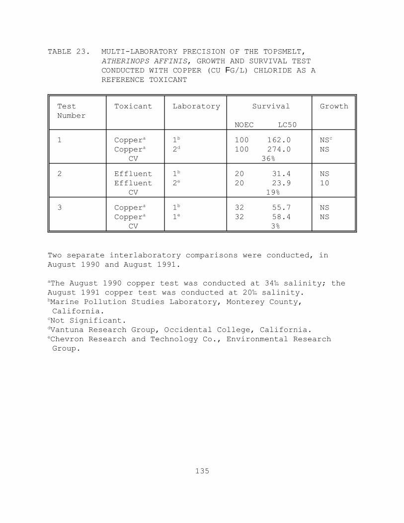
135

TABLE 23. MULTI-LABORATORY PRECISION OF THE TOPSMELT,ATHERINOPS AFFINIS, GROWTH AND SURVIVAL TESTCONDUCTED WITH COPPER (CU FG/L) CHLORIDE AS AREFERENCE TOXICANT

TestNumber

Toxicant Laboratory Survival

NOEC LC50

Growth

1 Coppera

Coppera

CV

1b

2d100 162.0100 274.0

36%

NScNS

2 EffluentEffluent CV

1b

2e20 31.420 23.9

19%

NS10

3 Coppera

Coppera

CV

1b

1e32 55.732 58.4

3%

NSNS

Two separate interlaboratory comparisons were conducted, inAugust 1990 and August 1991.

aThe August 1990 copper test was conducted at 34‰ salinity; the August 1991 copper test was conducted at 20‰ salinity.bMarine Pollution Studies Laboratory, Monterey County, California.cNot Significant.dVantuna Research Group, Occidental College, California.eChevron Research and Technology Co., Environmental Research Group.

136

APPENDIX I. TOPSMELT TEST: STEP-BY-STEP SUMMARY

PREPARATION OF TEST SOLUTIONS

A. Determine test concentrations and appropriate dilution waterbased on NPDES permit conditions and guidance from theappropriate regulatory agency.

B. Prepare effluent test solutions by diluting well mixedunfiltered effluent using volumetric flasks and pipettes. Use hypersaline brine where necessary to maintain all testsolutions at 34 ± 2‰. Include brine controls in tests thatuse brine.

C. Prepare a copper reference toxicant stock solution (10,000µg/L) by adding 0.0268 g of copper chloride (CuCl2N2H2O) to 1liter of reagent water.

D. Prepare zinc reference toxicant solution of 0 (control) 56,100, 180, and 180 µg/L by adding 0, 5.6, 10.0, 18.0, and 32.0 mL of stock solution, respectively, to a 1-L volumetricflask and filling to 1-L with dilution water.

E. Sample effluent and reference toxicant solutions forphysical/chemical analysis. Measure salinity, pH anddissolved oxygen from each test concentration.

F. Randomize numbers for test chambers and record the chambernumbers with their respective test concentrations on arandomization data sheet. Store the data sheet safely untilafter the test samples have been analyzed.

G. Place test chambers in a water bath or environmental chamberset to 20EC and allow temperature to equilibrate.

H. Measure the temperature daily in one random replicate (orseparate chamber) of each test concentration. Monitor thetemperature of the water bath or environmental chambercontinuously.

I. At the end of the test, measure salinity, pH, and dissolvedoxygen concentration from each test concentration.

137

PREPARATION AND ANALYSIS OF TEST ORGANISMS

A. Obtain 9-15 day old larvae from a commerical supplier or in-house cultures.

B. Larvae must be randomized before placing them into the testchambers. Be sure that all water used in culture, transfer,and test solutions is within 1EC of the test temperature.

C. Remove all dead larvae daily, and add 40 newly hatchedArtemia nauplii per larva twice daily; once in the morningand once in the afternoon. Adjust feeding to account forlarva mortality.

D. Renew test solutions daily using freshly prepared solutions,immediately after cleaning the test chambers.

E. After 7 days, count and record the number of live and deadlarvae in each chamber. After counting, use therandomization sheet to assign the correct test concentrationto each chamber. Remove all dead larvae.

F. The surviving larvae in each test chamber are immediatelyprepared as a group for dry weight determination, orpreserved in 4% formalin then 70% ethanol. Preservedorganisms are dried and weighed with 7 days.

G. Carefully transfer the larvae to a prenumbered, preweighedmicro-weigh boat using fine-tipped forceps. Dry for 24hours at 60EC or at 105EC for a minimum of 6 hours. Weigheach weigh boat on a microbalance (accurate to 1 µg). Record the chamber number, larvae weight, weigh boat weight(recorded previously), and number of larvae per weigh boat(replicate) on the data sheet.

H. Analyze the data.

I. Include standard reference toxicant point estimate values inthe standard quality control charts.

138

Data Sheet for Larval Fish Toxicity Test

Test Start Date: Start Time: Fish Species:

Test End Date: End Time: Collection/Arrival Date:

Reference Toxicant: Broodstock Source:

Fish Age at Start: TestCont. #

Concentration NumerAlive

TotalNumberAlive

TotalNumber atStart

Notes

Day1

Day2

Day3

Day 4 Day5

Day6

Day7

Computer Data StorageDiskFile

Note: See larval weight data on separate sheet.

139

Data Sheet for Weighing Larval Fish

Test Start Date: Start Time: Fish Species :

Test End Date: EndTime:

Collection/Arrival Date:

Toxicant: Fish Age at Start:

Sample Source:

Sample Type: Sediment Elutriate Porewater Water Test Container Number

Site Code orConcentration

Foil Number

Foil Weight (mg)

Total Weight (mg)

Weight ofLarval Fish

(mg)

Number of FishLarvae

Weight per Larval Fish (mg)

123456789

1011121314151617181920212223242526272829303132333435

Computer Data Storage NotesDisk:File:

Note: See larval mortality data on separate sheet.

140

SECTION 12

MYSID, Holmesimysis costataSURVIVAL AND GROWTH TEST METHOD

Adapted from a method developed byJohn W. Hunt, Brian S. Anderson and Sheila L. TurpenInstitute of Marine Sciences, University of California

Santa Cruz, California

(in association with)California Department of Fish and GameMarine Pollution Studies Laboratory

34500 Coast Route 1, Monterey, CA 93940

TABLE OF CONTENTS

12.1 Scope and Application12.2 Summary of Method12.3 Interferences12.4 Safety12.5 Apparatus and Equipment12.6 Reagents and Supplies12.7 Effluents and Receiving Water Collection,

Preservation, and Storage12.8 Calibration and Standardization12.9 Quality Control 12.10 Test Procedures12.11 Summary of Test Conditions and Test

Acceptability Criteria12.12 Acceptability of Test Results12.13 Data Analysis12.14 Precision and Accuracy

Appendix I Step-by Step Summary

141

SECTION 12

MYSID, HOLMESIMYSIS COSTATASURVIVAL AND GROWTH TEST

12.1 SCOPE AND APPLICATION

12.1.1 This method estimates the chronic toxicity of effluentsand receiving waters to the mysid, Holmesimysis costata, usingthree-to-four day old juveniles in a seven-day, static-renewalexposure. The effects include the synergistic, antagonistic,and additive effects of all chemical, physical, and additivecomponents which adversely affect the physiological andbiochemical functions of the test organisms.

12.1.2 Daily observations of mortality make it possible to alsocalculate acute toxicity for desired exposure periods (i.e., 24-h, 48-h, 96-h LC50s).

12.1.3 Detection limits of the toxicity of an effluent or a puresubstance are organism dependent.

12.1.4 Brief excursions in toxicity may not be detected using24-h composite samples. Also, because of the long samplecollection period involved in composite sampling and because testchambers are not sealed, highly volatile and highly degradabletoxicants present in the source may not be detected in the test.

12.1.5 This method is commonly used in one of two forms: (1) a definitive test, consisting of a minimum of five effluentconcentrations and a control, and (2) a receiving water test(s),consisting of one or more receiving water concentrations and acontrol.

12.1.6 This method should be restricted to use by, or under thesupervision of, professionals experienced in aquatic toxicitytesting. Specific experience with any toxicity test is usuallyneeded before acceptable results become routine.

12.2 SUMMARY OF METHOD

12.2.1 This method provides step-by-step instructions for

142

performing a 7-day static-renewal toxicity test using growth andsurvival juvenile mysids to determine the toxicity of substancesin marine waters. The test endpoints are survival and growth.

12.3 INTERFERENCES

12.3.1 Toxic substances may be introduced by contaminants indilution water, glassware, sample hardware, and testing equipment(see Section 5, Facilities, Equipment, and Supplies).

12.3.2 Improper effluent sampling and handling may adverselyaffect test results (see Section 8, Effluent and Receiving WaterSampling, Sample Handling, and Sample Preparation for ToxicityTests).

12.3.3 The test results can be confounded by (1) the presence ofpathogenic and/or predatory organisms in the dilution water,effluent, and receiving water, (2) the condition of the broodstock from which the test animals were taken, (3) the amount andtype of natural food in the effluent, receiving water, ordilution water, (4) nutritional value of the brine shrimp,Artemia nauplii, fed during the test, and (5) the quality of thebrine shrimp, Artemia nauplii, or other food added during thetest, which may sequester metals and other toxic substances, andlower the DO.

12.4 SAFETY

12.4.1 See Section 3, Health and Safety.

12.5 APPARATUS AND EQUIPMENT

12.5.1 Tanks, trays, or aquaria -- for holding and acclimatingadult mysids, e.g., standard salt water aquarium or Instant OceanAquarium (capable of maintaining seawater at 10-20EC), withappropriate filtration and aeration system.

12.5.2 Air pump, air lines, and air stones -- for aerating watercontaining mysids for supplying air to test solutions with lowdissolved oxygen.

12.5.3 Constant temperature chambers or water baths -- formaintaing test solution temperature and keeping dilution water

143

supply, juvenile mysids, and stock suspensions at testtemperature (13 or 15EC) prior to the test.

12.5.4 Water purification system -- Millipore Super-Q, Deionizedwater (DI) or equivalent.

12.5.5 Refractometer -- for determining salinity.

12.5.6 Hydrometer(s) -- for calibrating refractometer.

12.5.7 Thermometers, glass or electronic, laboratory grade --for measuring water temperatures.

12.5.8 Thermometer, National Bureau of Standards Certified (seeUSEPA METHOD l70.l, USEPA, l979) -- to calibrate laboratorythermometers.

12.5.9 pH and DO meters -- for routine physical and chemicalmeasurements.

12.5.10 Standard or micro-Winkler apparatus -- for determiningDO (optional) and calibrating the DO meter.

12.5.11 Winkler bottles -- for dissolved oxygen determinations.

12.5.12 Balance -- Analytical, capable of accurately weighing to0.0001 g (for weighing reference toxicants).

12.5.13 Microbalance -- Analytical, capable of accuratelyweighing to 0.000001 g (for weighing mysids).

12.5.14 Fume hood -- to protect the analyst from effluent orformaldehyde fumes.

12.5.15 Glass stirring rods -- for mixing test solutions.

12.5.16 Graduated cylinders -- Class A, borosilicate glass ornon-toxic plastic labware, 50-l000 mL for making test solutions.

12.5.17 Volumetric flasks -- Class A, borosilicate glass or non-toxic plastic labware, 10-1000 mL for making test solutions.

12.5.18 Pipets, automatic -- adjustable, to cover a range of

144

delivery volumes from 0.010 to 100 mL.

12.5.19 Pipet bulbs and fillers -- PROPIPET® or equivalent.

12.5.20 Wash bottles -- for reagent water, for topping offgraduated cylinders, for rinsing small glassware and instrumentelectrodes and probes.

12.5.21 Wash bottles -- for dilution water.

12.5.22 20-liter cubitainers or polycarbonate water cooler jugs-- for making hypersaline brine.

12.5.23 Cubitainers, beakers, or similar chambers of non-toxiccomposition for holding, mixing, and dispensing dilution waterand other general non-effluent, non-toxicant contact uses. Theseshould be clearly labeled and not used for other purposes.

12.5.24 Pipets, volumetric: 1, 10, 25, 50, and 100 mL -- fordilutions.

12.5.25 Plastic randomization cups (approximately 100 mL, onefor each test chamber).

12.5.26 Brine shrimp, Artemia, culture unit -- see Subsection12.6.24 and Section 4, Quality Assurance.

12.5.27 Separatory funnels, 2-L -- two to four for culturingArtemia.

12.5.28 Mysid culture apparatus (see Section 12.6.25.5). Thistest requires 400 three- to four-day-old juvenile mysids.

12.5.29 Gear for collecting adult mysids, including a smallboat, 0.5 mm-mesh hand nets, plastic buckets, and portable airsupply (mysids may also be obtained from commercial suppliers;).

12.5.30 Pipet bulbs and glass tubes (4 mm diameter, with fire-polished edges) for handling adult mysids.

12.5.31 Siphon tubes (fire polished glass with attached siliconetubing) -- for test solution renewals.

145

12.5.32 Fire-polished wide-bore 10 mL pipet -- for handlingjuveniles.

12.5.33 Forceps with fine points -- for transferring juvenilesto weighing pans.

12.5.34 Light box -- for examining organisms.

12.5.35 Drying oven, 50-105EC range -- for drying organisms.

12.5.36 Desiccator -- for holding dried organisms.

12.5.37 Clean NITEX® mesh sieves (# 150 µm, 500-1000µm) -- forconcentrating organisms. (NITEX® is available from SterlingMarine Products, 18 Label Street, Montclair, NJ 07042; 201-783-9800).

12.5.38 60 µm NITEX® filter - for filtering receiving water.

12.6 REAGENTS AND SUPPLIES

12.6.1 Sample containers -- for sample shipment and storage (seeSection 8, Effluent and Receiving Water Sampling, and SampleHandling, and Sample Preparation for Toxicity Tests).

12.6.2 Data sheets (one set per test) -- for data recording(Figures 1 and 2).

12.6.3 Tape, colored -- for labelling test chambers andcontainers.

12.6.4 Markers, water-proof -- for marking containers, etc.

12.6.5 Parafilm -- to cover graduated cylinders and vessels.

12.6.6 Gloves, disposable -- for personal protection fromcontamination.

12.6.7 Pipets, serological -- l-l0 mL, graduated.

12.6.8 Pipet tips -- for automatic pipets.

12.6.9 Coverslips -- for microscope slides.

146

12.6.10 Lens paper -- for cleaning microscope optics.

12.6.11 Laboratory tissue wipes -- for cleaning and dryingelectrodes, microscope slides, etc.

12.6.12 Disposable countertop covering -- for protection of worksurfaces and minimizing spills and contamination.

12.6.13 pH buffers 4, 7, and l0 (or as per instructions ofinstrument manufacturer) -- for standards and calibration check(see USEPA Method l50.l, USEPA, l979).

12.6.14 Membranes and filling solutions -- for dissolved oxygenprobe (see USEPA Method 360.l, USEPA, l979), or reagents formodified Winkler analysis.

12.6.15 Laboratory quality assurance samples and standards --for the above methods.

12.6.16 Test chambers -- 1000 mL, five chambers perconcentration. The chambers should be borosilicate glass (foreffluents) or nontoxic disposable plastic labware (for referencetoxicants). To avoid contamination from the air and excessiveevaporation of test solutions during the test, the chambersshould be covered during the test with safety glass plates or aplastic sheet (6 mm thick).

12.6.17 Micro-weighing pans, aluminum -- to determine the dryweight of organisms. Weighting pan should be about 5 mg or lessto minimize noise in measurement of the small mysids.

12.6.18 Fronds of kelp (Macrocystis) for habitat in culture.

12.6.19 Reference toxicant solutions (see Subsection 12.10.2.4and see Section 4, Quality Assurance).

12.6.20 Reagent water -- defined as distilled or deionized waterthat does not contain substances which are toxic to the testorganisms (see Section 5, Facilities, Equipment, and Supplies andSection 7, Dilution Water).

147

12.6.21 Effluent and receiving water -- see Section 8, Effluentand Surface Water Sampling, and Sample Handling, and SamplePreparation for Toxicity Tests.

12.6.22 Dilution water and hypersaline brine -- see Section 7,Dilution Water and Section 12.6.24, Hypersaline Brines. Thedilution water should be uncontaminated 1-µm-filtered naturalseawater. Hypersaline brine should be prepared from dilutionwater.

12.6.23 HYPERSALINE BRINES

12.6.23.1 Most industrial and sewage treatment effluentsentering marine and estuarine systems have little measurablesalinity. Exposure of larvae to these effluents will usuallyrequire increasing the salinity of the test solutions. It isimportant to maintain an essentially constant salinity across alltreatments. In some applications it may be desirable to matchthe test salinity with that of the receiving water (See Section7.1). Two salt sources are available to adjust salinities --artificial sea salts and hypersaline brine (HSB) derived fromnatural seawater. Use of artificial sea salts is necessary onlywhen high effluent concentrations preclude salinity adjustment byHSB alone.

12.6.23.2 Hypersaline brine (HSB) can be made by concentratingnatural seawater by freezing or evaporation. HSB should be madefrom high quality, filtered seawater, and can be added to theeffluent or to reagent water to increase salinity. HSB hasseveral desirable characteristics for use in effluent toxicitytesting. Brine derived from natural seawater contains thenecessary trace metals, biogenic colloids, and some of themicrobial components necessary for adequate growth, survival,and/or reproduction of marine and estuarine organisms, and it canbe stored for prolonged periods without any apparent degradation. However, even if the maximum salinity HSB (100‰) is used as adiluent, the maximum concentration of effluent (0‰) that can betested is 66% effluent at 34‰ salinity (see Table 1).

12.6.23.3 High quality (and preferably high salinity) seawatershould be filtered to at least 10 µm before placing into thefreezer or the brine generator. Water should be collected on anincoming tide to minimize the possibility of contamination.

148

12.6.23.4 Freeze Preparation of Brine

12.6.23.4.1 A convenient container for making HSB by freezing isone that has a bottom drain. One liter of brine can be made fromfour liters of seawater. Brine may be collected by partiallyfreezing seawater at -10 to -20EC until the remaining liquid hasreached the target salinity. Freeze for approximately six hours,then separate the ice (composed mainly of fresh water) from theremaining liquid (which has now become hypersaline).

12.6.23.4.2 It is preferable to monitor the water until thetarget salinity is achieved rather than allowing total freezingfollowed by partial thawing. Brine salinity should never exceed 100‰. It is advisable not to exceed about 70‰ brine salinityunless it is necessary to test effluent concentrations greaterthan 50%.

12.6.23.4.3 After the required salinity is attained, the HSBshould be filtered through a 1 µm filter and poured directly intoportable containers (20-L cubitainers or polycarbonate watercooler jugs are suitable). The brine storage containers shouldbe capped and labelled with the salinity and the date the brinewas generated. Containers of HSB should be stored in the dark at4EC (even room temperature has been acceptable). HSB is usuallyof acceptable quality even after several months in storage.

12.6.23.5 Heat Preparation of Brine

12.6.23.5.1 The ideal container for making brine using heat-assisted evaporation of natural seawater is one that (1) has ahigh surface to volume ratio, (2) is made of a non-corrosivematerial, and (3) is easily cleaned (fiberglass containers areideal). Special care should be used to prevent any toxicmaterials from coming in contact with the seawater being used togenerate the brine. If a heater is immersed directly into theseawater, ensure that the heater materials do not corrode or leach any substances that would contaminate the brine. Onesuccessful method is to use a thermostatically controlled heatexchanger made from fiberglass. If aeration is needed, use onlyoil-free air compressors to prevent contamination. 12.6.23.5.2 Before adding seawater to the brine generator,thoroughly clean the generator, aeration supply tube, heater, and

149

any other materials that will be in direct contact with thebrine. A good quality biodegradable detergent should be used,followed by several (at least three) thorough reagent waterrinses.

TABLE 1. MAXIMUM EFFLUENT CONCENTRATION (%) THAT CAN BE TESTED AT 34‰ WITHOUT THE ADDITION OF DRY SALTS GIVEN THE INDICATED EFFLUENT AND BRINE SALINITIES.

Effluent Brine Brine Brine Brine Brine

Salinity‰

60‰

70‰

80‰

90‰

100‰

0 43.33 51.43 57.50 62.22 66.00

1 44.07 52.17 58.23 62.92 66.67

2 44.83 52.94 58.97 63.64 67.35

3 45.61 53.73 59.74 64.37 68.04

4 46.43 54.55 60.53 65.12 68.75

5 47.27 55.38 61.33 65.88 69.47

10 52.00 60.00 65.71 70.00 73.33

15 57.78 65.45 70.77 74.67 77.65

20 65.00 72.00 76.67 80.00 82.50

25 74.29 80.00 83.64 86.15 88.00

12.6.23.5.3 Seawater should be filtered to at least 10 µm beforebeing put into the brine generator. The temperature of theseawater is increased slowly to 40EC. The water should beaerated to prevent temperature stratification and to increasewater evaporation. The brine should be checked daily (dependingon the volume being generated) to ensure that the salinity doesnot exceed 100‰ and that the temperature does not exceed 40EC. Additional seawater may be added to the brine to obtain thevolume of brine required.

12.6.23.5.4 After the required salinity is attained, the HSB

150

should be filtered through a 1 µm filter and poured directly intoportable containers (20-L cubitainers or polycarbonate watercooler jugs are suitable). The brine storage containers shouldbe capped and labelled with the salinity and the date the brinewas generated. Containers of HSB should be stored in the dark at4EC (even room temperature has been acceptable). HSB is usuallyof acceptable quality even after several months in storage.

12.6.23.6 Artificial Sea Salts

12.6.23.6.1 No data from mysids using sea salts or artificialseawater (e.g., GP2) are available for evaluation at this time,and their use must be considered provisional.

12.6.23.7 Dilution Water Preparation from Brine

12.6.23.7.1 Although salinity adjustment with brine is thepreferred method, the use of high salinity brines and/or reagentwater has sometimes been associated with discernible adverseeffects on test organisms. For this reason, it is recommendedthat only the minimum necessary volume of brine and reagent waterbe used to offset the low salinity of the effluent, and thatbrine controls be included in the test. The remaining dilutionwater should be natural seawater. Salinity may be adjusted inone of two ways. First, the salinity of the highest effluenttest concentration may be adjusted to an acceptable salinity, andthen serially diluted. Alternatively, each effluentconcentration can be prepared individually with appropriatevolumes of effluent and brine.

12.6.23.7.2 When HSB and reagent water are used, thoroughlymix together the reagent water and HSB before mixing in theeffluent. Divide the salinity of the HSB by the expected testsalinity to determine the proportion of reagent water to brine. For example, if the salinity of the brine is 100‰ and the test isto be conducted at 34‰, 100‰ divided by 34‰ = 2.94. Theproportion of brine is 1 part, plus 1.94 parts reagent water. Tomake 1 L of dilution water at 34‰ salinity from a HSB of 100‰,340 mL of brine and 660 mL of reagent water are required. Verifythe salinity of the resulting mixture using a refractometer.

12.6.23.8 Test Solution Salinity Adjustment

151

12.6.23.8.1 Table 2 illustrates the preparation of testsolutions (up to 50% effluent) at 34‰ by combining effluent, HSB,and dilution water. Note: if the highest effluent concentrationdoes not exceed 50% effluent, it is convenient to prepare brineso that the sum of the effluent salinity and brine salinityequals 68‰; the required brine volume is then always equal to theeffluent volume needed for each effluent concentration as in theexample in Table 2. 12.6.23.8.2 Check the pH of all brine mixtures and adjust towithin 0.2 units of dilution water pH by adding, dropwise, dilutehydrochloric acid or sodium hydroxide(see Section 8.8.9, Effluentand Receiving Water Sampling, Sample Handling, and SamplePreparation for Toxicity Tests).

12.6.23.8.3 To calculate the amount of brine to add to eacheffluent dilution, determine the following quantities: salinityof the brine (SB, in ‰), the salinity of the effluent (SE, in ‰),and volume of the effluent to be added (VE, in mL). Then use thefollowing formula to calculate the volume of brine (VB, in mL) tobe added:

VB = VE x (34 - SE)/(SB - 34)

12.6.23.8.4 This calculation assumes that dilution watersalinity is 34 ± 2‰.

12.6.23.9 Preparing Test Solutions

12.6.23.9.1 Two hundred mL of test solution are needed for eachtest chamber. To prepare test solutions at low effluentconcentrations (<6%), effluents may be added directly to dilutionwater. For example, to prepare 1% effluent, add 10 mL ofeffluent to a 1-liter volumetric flask using a volumetric pipetor calibrated automatic pipet. Fill the volumetric flask to the1-liter mark with dilution water, stopper it, and shake to mix. Distribute equal volumes into the replicate test chambers.

12.6.23.9.2 To prepare a test solution at higher effluentconcentrations, hypersaline brine must usually be used. Forexample, to prepare 40% effluent, add 400 mL of effluent to a 1-liter volumetric flask. Then, assuming an effluent salinity of2‰ and a brine salinity of 66‰, add 400 mL of brine (see

152

equation above and Table 2) and top off the flask with dilutionwater. Stopper the flask and shake well. Distribute equalvolumes into the replicate test chambers.

12.6.23.10 Brine Controls

12.6.23.10.1 Use brine controls in all tests where brine isused. Brine controls contain the same volume of brine as doesthe highest effluent concentration using brine, plus the volumeof reagent water needed to reproduce the hyposalinity of theeffluent in the highest concentration, plus dilution water. Calculate the amount of reagent water to add to brine controls byrearranging the above equation, (See, 12.6.23.8.3) setting SE =0, and solving for VE.

VE = VB x (SB - 34)/(34 - SE)

If effluent salinity is essentially 0‰, the reagent water volumeneeded in the brine control will equal the effluent volume at thehighest test concentration. However, as effluent salinity andeffluent concentration increase, less reagent water volume isneeded.

12.6.24 BRINE SHRIMP, ARTEMIA SP., NAUPLII -- for feedingcultures and test organisms.

12.6.24.1 Newly hatched Artemia sp. nauplii are used for foodfor the stock cultures and test organisms. Although there aremany commercial sources of brine shrimp cysts, the Brazilian orColombian strains are preferred because the supplies examinedhave had low concentrations of chemical residues and producenauplii of suitably small size. (One source that has been foundto be acceptable is Aquarium Products, 180L Penrod Ct., GlenBurnie, Maryland 21061). For commercial sources of brine shrimp,Artemia, cysts, see Table 2 of Section 5, Facilities, Equipment,and Supplies); and Section 4, Quality Assurance.

12.6.24.2 Each new batch of Artemia cysts should be evaluatedfor size (Vanhaecke and Sorgeloos, 1980, and Vanhaecke et al.,1980) and nutritional suitability (Leger, et al., 1985, Leger, etal., 1986) against known suitable reference cysts by performing aside-by-side larval growth test using the "new" and "reference"cysts. The "reference" cysts used in the suitability test may be

153

a previously tested and acceptable batch of cysts, or may beobtained from the Quality Assurance Research Division, EMSL,Cincinnati, OH 45268, 513-569-7325. A sample of newly-hatchedArtemia nauplii from each new batch of cysts should be chemicallyanalyzed. The Artemia cysts should not be used if theconcentration of total organochlorine pesticides 0.15 ug/g wetweight or that the total concentration of organochlorinepesticides plus PCBs exceeds 0.30 µg/g wet weight (For analyticalmethods see USEPA, 1982).

12.6.24.3 Artemia nauplii are obtained as follows:

1. Add 1 L of seawater, or an aqueous unionized salt(NaCl) solution prepared with 35 g salt or artificialsea salts per liter, to a 2-L separatory funnel, orequivalent.

2. Add 10 mL Artemia cysts to the separatory funnel andaerate for 24 h at 27EC. Hatching time varies withincubation temperature and the geographic strain ofArtemia used (see USEPA, 1985a; USEPA, 1993a; ASTM,1993).

3. After 24 h, cut off the air supply in the separatoryfunnel. Artemia nauplii are phototactic, and willconcentrate at the bottom of the funnel if it iscovered for 5-10 minutes with a dark cloth or papertowel. To prevent mortality, do not leave theconcentrated nauplii at the bottom of the funnel morethan 10 min without aeration.

4. Drain the nauplii into a funnel fitted with a #150 µmNITEX® or stainless steel screen, and rinse withseawater or equivalent before use.

12.6.24.4 Testing Artemia nauplii as food for toxicity testorganisms.

12.6.24.4.1 The primary criteria for acceptability of each newsupply of brine shrimp cysts is adequate survival, and growth ofthe mysids. The mysids used to evaluate the acceptability of thebrine shrimp nauplii must be the same geographical origin andstage of development (3 to 4 days old) as those used routinely inthe toxicity tests. Two 7-day chronic tests are performed side-by-side, each consisting of five replicate test vesselscontaining five juveniles (25 organisms per test, total of 50

154

TABLE 2. EXAMPLES OF EFFLUENT DILUTION SHOWING VOLUMES OFEFFLUENT (x‰), BRINE, AND DILUTION WATER NEEDED FOR ONELITER OF EACH TEST SOLUTION.

FIRST STEP: Combine brine with deionized water or natural seawater to achievea brine of 68-x‰ and, unless natural seawater is used for dilution water, alsoa brine-based dilution water of 34‰.

SERIAL DILUTION:

Step 1. Prepare the highest effluent concentration to be tested by addingequal volumes of effluent and brine to the appropriate volume of dilutionwater. An example using 40% is shown.

Effluent Conc.(%)

Effluent x‰ Brine (68-x)‰

Dilution Water*34‰

40 800 mL 800 mL 400 mLStep 2. Use either serially prepared dilutions of the highest testconcentration or individual dilutions of 100% effluent.

Effluent Conc. (%) Effluent Source Dilution Water* (34‰)

20 1000 mL of 40% 1000 mL

10 1000 mL of 20% 1000 mL

5 1000 mL of 10% 1000 mL

2.5 1000 mL of 5% 1000 mL

Control none 1000 mLINDIVIDUAL PREPARATION

Effluent Conc.(%)

Effluent x‰ Brine (68-x)‰ Dilution Water*34‰

40 400 mL 400 mL 200 mL

20 200 mL 200 mL 600 mL

10 100 mL 100 mL 800 mL

5 50 mL 50 mL 900 mL

2.5 25 mL 25 mL 950 mL

Control none none 1000 mL

*May be natural seawater or brine-reagent water equivalent.

155

organisms). The juveniles in one set of test chambers is fedreference (acceptable) nauplii and the other set is fed naupliifrom the "new" source of Artemia cysts.

12.6.24.4.2 The feeding rate and frequency, test vessels, volumeof control water, duration of the tests, and age of the Artemianauplii at the start of the test, should be the same as used forthe routine toxicity tests.

12.6.24.4.3 Results of the brine shrimp, Artemia, naupliinutrition assay, where there are only two treatments, can beevaluated statistically by use of a t test. The "new" food isacceptable if there are no statistically significant differencesin the survival or growth of the mysids fed the two sources ofnauplii.

12.6.25 TEST ORGANISMS

12.6.25.1 The test organisms for this method are juveniles ofthe mysid crustacean, Holmesimysis costata (Holmes 1900;previously referred to as Acanthomysis sculpta). H. costataoccurs in the surface canopy of the giant kelp Macrocystispyrifera where it feeds on zooplankters, kelp, epiphytes, anddetritus. There are few references to the ecology of this mysidspecies (Holmquist, 1979; Clutter, 1967, 1969; Green, 1970;Turpen et al., 1994). H. costata is numerically abundant in kelpforest habitats and is considered to be an important food sourcefor kelp forest fish (Clark 1971, Mauchline 1980). Mysids arecalled opossum shrimp because females brood their young in anabdominal pouch, the marsupium. H. costata eggs develop forabout 20 days in the marsupium before the young are released asjuveniles; broods are released at night during molting. Femalesrelease their first brood at 55 to 70 days post-release (at12EC), and may have multiple broods throughout theirapproximately 120-day life.

12.6.25.2 H. costata has been used in previous toxicity studieswith a variety of toxicants (Tatem and Portzer, 1985; Davidson etal., 1986; Machuzac and Mikel, 1987; Reish and Lemay, 1988;Asato, 1988; Martin et al., 1989; Singer et al., 1990; 1991; Huntet al., In Press). Mysids are useful as toxicity test organismsbecause of their widespread availability, ecological importance,sensitivity to toxicants, and amenability to laboratory culture

156

(Nimmo et al., 1977; Mauchline, 1980; Gentile et al., 1982;Lussier et al., 1985).

12.6.25.3 Species Identification

12.6.25.3.1 Laboratories unfamiliar with the test organismshould collect preliminary samples to verify speciesidentification. Refer to Holmquist (1979) or send samples ofmysids and any similar co-occurring organisms to a qualifiedtaxonomist. Request certification of species identification fromany organism suppliers. Records of verification should bemaintained along with a few preserved specimens.

12.6.25.3.2 There have been recent revisions to the taxonomy ofH. costata. Previous authors have referred to this species asAcanthomysis sculpta. However, Holmquist's (1979) reviewconsiders previous references to Acanthomysis sculpta inCalifornia to be synonymous with Holmesimysis costata; weconsider Holmquist's designation to be definitive.

12.6.25.4 Obtaining Broodstock

12.6.25.4.1 H. costata can be collected by sweeping a small-mesh(0.5 - 1 mm) hand net through the water just under the surfacecanopy blades of giant kelp Macrocystis pyrifera. Although thismethod collects mysids of all sizes, attention should be paid tothe number of gravid females collected because these are used toproduce the juvenile mysids used in toxicity testing. Mysidsshould be collected from waters remote from sources of pollutionto minimize the possibility of physiological or geneticadaptation to toxicants.

12.6.25.4.2 Mysids can be transported for a short time (< 3hours) in tightly covered 20 liter plastic buckets. The bucketsshould be filled to the top with seawater from the collectionsite, and should be gently aerated or oxygenated to maintaindissolved oxygen above 60% saturation. Transport temperaturesshould remain within 3EC of the temperature at the collectionsite.

12.6.25.4.3 For longer transport times of up to 36 hours, mysidscan be shipped in sealed plastic bags filled with seawater. Thefollowing transport procedure has been used successfully: 1)

157

fill the plastic bag with one liter of dilution water seawater,2) saturate the seawater with oxygen by bubbling pure oxygen forat least 10 minutes, 3) place 25-30 adult mysids, or up to 100juvenile mysids in each bag, 4) for adults add about 20 Artemianauplii per mysid, for 100 juveniles add a pinch (10 to 20 mg) ofground Tetramin® flake food and 200 newly-hatched Artemianauplii, 5) seal the bag securely, eliminating any airspace, then6) place it within a second sealed bag in an ice chest. Do notoverfeed mysids in transport, as this may deplete dissolvedoxygen, causing stress or mortality in transported mysids. Awell insulated ice chest should be cooled to approximately 15ECby adding one 1-liter blue ice block for every five 1-liter bagsof mysids (a temperature range of 12 to 16EC is tolerable). Wrapthe ice in newspaper and a plastic bag to insulate it from themysid bags. Pack the bags tightly to avoid shifting within thecooler.

12.6.25.5 Broodstock Culture and Handling

12.6.25.5.1 After collection, the mysids should be transporteddirectly to the laboratory and placed in seawater tanks oraquaria equipped with flowing seawater or adequate aeration andfiltration. Initial flow rates should be adjusted so that anytemperature change occurs gradually (0.5EC per hour). The watertemperature should be held at 15 ± 1EC. Note: Mysids collectednorth of Pt. Conception, California, should be held and tested at13 ± 1EC.

12.6.25.5.2 Mysids can be cultured in tanks ranging from 4 to1000 liters. Tanks should be equipped with gentle aeration andblades of Macrocystis to provide habitat. Static culture tankscan be used if there is constant aeration, temperature control,and frequent water changes (one half the water volume changed atleast twice a week). Maintain culture density below 20 animalsper liter by culling out adult males or juveniles.

12.6.25.5.3 Adult mysids should be fed 100 Artemia nauplii permysid per day. Juveniles should be fed 5 to 10 newly releasedArtemia nauplii per juvenile per day and a pinch (10 to 20 mg) ofground Tetramin® flake food per 100 juveniles per day. Staticchambers should be carefully monitored and rations adjusted to

158

prevent overfeeding and fouling of culture water. Refer tosection 12.6.19 for details of Artemia culture and qualitycontrol.

12.6.25.6 Culture Materials

12.6.25.6.1 Refer to Section 5, Facilities and Equipment, for adiscussion of suitable materials to be used in laboratory cultureof mysids. Be sure all new materials are properly leached inseawater before use. After use, all culture materials should bewashed in soap and water, then rinsed with seawater before re-use.

12.6.25.7 Test Organisms

12.6.25.7.1 Approximately 150 gravid female mysids should beisolated to provide approximately 400 juveniles for each set oftoxicity tests (5 juveniles/chamber x 30 reference toxicantchambers and approximately 35 effluent chambers, plus additionalmysids so that only healthy active juveniles are used in thetest). Gravid females can be identified by their large, extendedmarsupia filled with (visible) eyed juveniles. Marsupia appeardistended and gray when females are ready to release young, dueto presence of the juveniles.

12.6.25.7.2 Gravid females are easily isolated from other mysidsusing the following technique: (1) use a small dip net tocapture about 100 mysids from the culture tank, (2)transfer themysids to a screen-bottomed plastic tube (150 µm-mesh, 25-cmdiam.) partly immersed in a water bath or bucket, (3)lift thescreen-tube out of the water to immobilize mysids on the dampscreen, (4)gently draw the gravid females off the screen with asuction bulb and fire-polished glass tube (5-mm bore), (5) collect the gravid females in a separate screen tube. Re-immersethe screen continuously during the isolation process; mysidsshould not be exposed to air for more than a few seconds at atime.

12.6.25.7.3 Four or five days before a toxicity test begins,transfer gravid females into a removable, 2-mm-mesh screenedcradle suspended within an aerated 80-liter aquarium. Beforetransfer, make sure there are no juveniles in with the adultfemales. Extraneous juveniles are excluded to avoid

159

inadvertently mixing them with the soon-to-be released juvenilesused in testing. Provide the gravid females with newly hatchedArtemia nauplii (approximately 200 per mysid) to help stimulatejuvenile release. Artemia can be provided continuouslythroughout the night from an aerated reservoir holdingapproximately 75,000 Artemia. Direct the flow from the feederinto the screened compartment with the females, and add a fewblades of Macrocystis for habitat. The females are placed withinthe screened compartment so that as the juveniles are released,they can swim through the mesh into the bottom of the aquarium. Outflows on flow-through aquaria should be screened (150-µm-mesh)to retain juveniles and allow some Artemia to escape.

12.6.25.7.4 Juveniles are generally released at night, so it isimportant to turn off all lights at night to promote release. Inthe morning, the screened compartment containing the femalesshould be removed and placed in a separate aquarium. Juvenilesshould be slowly siphoned through a wide-diameter hose into a150-µm-mesh screen-bottom tube (25 cm diam.) immersed in a bucketfilled with clean seawater. Once the release aquarium isemptied, it should be washed with hot fresh water to eliminatestray juveniles that might mix with the next cohort.

12.6.25.7.5 After collection, the number of juveniles should beestimated visually or by counting subsamples with a small beaker. If there are not enough juveniles to conduct the necessary tests,they can be mixed with juveniles from one previous or subsequentrelease so that the test is initiated with three and/or four-dayold juveniles. Initial experiments indicate that mysids 2-days-old and younger survive poorly in toxicity tests and that mysidsolder than four days may vary in their toxicant sensitivity orsurvival rate (Hunt et al., 1989; Martin et al., 1989).

12.6.25.7.6 Test juveniles should be transferred to additionalscreen-tubes (or to 4-liter static beakers if flowing seawater isunavailable). The screen-tubes are suspended in a 15-literbucket so that dilution water seawater (0.5 liter/min) can flowinto the tube, through the screen, and overflow from the bucket. Check water flow rates (< one liter/min) to make sure thatjuveniles or Artemia nauplii are not forced down onto the screen. The height of the bucket determines the level of water in thescreen tube. About 200 to 300 juveniles can be held in eachscreen-tube (200 juveniles per static 4-liter beaker). Juveniles

160

should be fed 40 newly hatched Artemia nauplii per mysid per dayand a pinch (10 to 20 mg) of ground Tetramin® flake food per 100juveniles per day. A blade of Macrocystis (well rinsed inseawater) should be added to each chamber. Chambers should begently aerated and temperature controlled at 15 ± 1EC (or 13 ±1EC if collected north of Pt. Conception). Half of the seawaterin static chambers should be changed at least once betweenisolation and test initiation.

12.6.25.7.7 The day juveniles are isolated is designated day 0(the morning after their nighttime release). The toxicity testshould begin on day three or four. For example, if juveniles areisolated on Friday, the toxicity test should begin on thefollowing Monday or Tuesday.

12.7 EFFLUENT AND RECEIVING WATER COLLECTION, PRESERVATION, AND STORAGE

12.7.1 See Section 8, Effluent and Receiving Water Sampling,Sample Handling, and Sample Preparation for Toxicity Tests.

12.8 CALIBRATION AND STANDARIZATION

12.8.1 See Section 4, Quality Assurance.

12.9 QUALITY CONTROL

12.9.1 See Section 4, Quality Assurance.

12.10 TEST PROCEDURES

12.10.1 TEST DESIGN

12.10.1.1 The test consists of at least five effluentconcentrations plus a dilution water control. Tests that usebrine to adjust salinity must also contain five replicates of abrine control.

12.10.1.2 Effluent concentrations are expressed as percenteffluent.

12.10.2 TEST SOLUTIONS

161

12.10.2.1 Receiving waters

12.10.2.1.1 The sampling point is determined by the objectivesof the test. At estuarine and marine sites, samples are usuallycollected at mid-depth. Receiving water toxicity is determinedwith samples used directly as collected or with samples passedthrough a 60 µm NITEX® filter and compared without dilution,against a control. Using five replicates chambers per test, eachcontaining 200 mL would require approximately 1 L or more ofsample per test per renewal.

12.10.2.2 Effluents

12.10.2.2.1 The selection of the effluent test concentrationsshould be based on the objectives of the study. A dilutionfactor of at least 0.5 is commonly used. A dilution factor of0.5 provides hypothesis test discrimination of ± 100%, andtesting of a 16 fold range of concentrations. Hypothesis testdiscrimination shows little improvement as dilution factors areincreased beyond 0.5 and declines rapidly if smaller dilutionfactors are used. USEPA recommends that one of the five effluenttreatments must be a concentration of effluent mixed withdilution water which corresponds to the permittee's instreamwaste concentration (IWC). At least two of the effluenttreatments must be of lesser effluent concentration than the IWC,with one being at least one-half the concentration of the IWC. If 100‰ HSB is used as a diluent, the maximum concentration ofeffluent that can be tested will be 66% at 34‰ salinity.

12.10.2.2.2 If the effluent is known or suspected to be highlytoxic, a lower range of effluent concentrations should be used(such as 25%, 12.5%, 6.25%, 3.12% and 1.56%).

12.10.2.2.3 The volume of effluent required for a 75% renewal offive replicates per concentration for five concentrations ofeffluent and two controls, each containing 200 mL of testsolution, is approximately 370 mL.

12.10.2.2.4 Effluent dilutions should be prepared for allreplicates in each treatment in one container to minimizevariability among the replicates. Dispense into the appropriateeffluent test chambers.

162

12.10.2.3 Dilution Water

12.10.2.3.1 Dilution water should be uncontaminated 1-µm-filtered natural seawater or hypersaline brine prepared fromuncontaminated natural seawater plus reagent water (see Section7, Dilution Water). Natural seawater may be uncontaminatedreceiving water. This water is used in all dilution steps and asthe control water.

12.10.2.4 Reference Toxicant Test

12.10.2.4.1 Reference toxicant tests should be conducted asdescribed in Quality Assurance (see Section 4.7).

12.10.2.4.2 The preferred reference toxicant for mysids is zincsulfate (ZnSO4N7H2O). Reference toxicant tests provide anindication of the sensitivity of the test organisms and thesuitability of the testing laboratory (see Section 4 QualityAssurance). Another toxicant may be specified by the appropriateregulatory agency. Prepare a 10,000 µg/L zinc stock solution byadding 0.0440 g of zinc sulfate (ZnSO4N7H2O) to one liter ofreagent water in a polyethylene volumetric flask. Alternatively,certified standard solutions can be ordered from commercialcompanies.

12.10.2.4.3 Reference toxicant solutions should be fivereplicates each of 0 (control), 10, 18, 32, and 56, and 100 µg/Ltotal zinc. Prepare one liter of each concentration by adding 0,1.0, 1.8, 3.2, 5.6, and 10.0 mL of stock solution, respectively,to one-liter volumetric flasks and fill with dilution water. Start with control solutions and progress to the highestconcentration to minimize contamination.

12.10.2.4.4 If the effluent and reference toxicant tests are tobe run concurrently, then the tests must use juvenile originatingfrom or released from the same pool of gravid females. The testsmust be handled in the same way and test solutions delivered tothe test chambers at the same time. Reference toxicant testsmust be conducted at 34 ± 2‰.

12.10.3 START OF THE TEST

12.10.3.1 Prior to Beginning the Test

163

12.10.3.1.1 The test should begin as soon as possible, preferably within 24 h of sample collection. The maximum holdingtime following retrieval of the sample from the sampling deviceshould not exceed 36 h for off-site toxicity tests unlesspermission is granted by the permitting authority. In no caseshould the sample be used in a test more than 72 h after samplecollection (see Section 8 Effluent and Receiving Water Sampling,Sample Handling, and Sample Preparation for Toxicity Test).

12.10.3.1.2 Just prior to test initiation (approximately 1 h),the temperature of a sufficient quantity of the sample to makethe test solutions should be adjusted to the test temperature (13or 15 ± 1EC) and maintained at that temperature during theaddition of dilution water.

12.10.3.1.3 Increase the temperature of the water bath, room, orincubator to the required test temperature (13 or 15 ± 1EC).

12.10.3.1.4 Randomize the placement of test chambers in thetemperature-controlled water bath, room, or incubator at thebeginning of the test, using a position chart. Assign numbersfor the position of each test chamber using a random numbers orsimilar process (see Appendix A, for an example ofrandomization). Maintain the chambers in this configurationthroughout the test, using a position chart. Record thesenumbers on a separate data sheet together with the concentrationand replicate numbers to which they correspond. Identify thissheet with the date, test organism, test number, laboratory, andinvestigator's name, and safely store it away until after themysids have been examined at the end of the test.

12.10.3.1.5 Note: Loss of the randomization sheet wouldinvalidate the test by making it impossible to analyze the data afterwards. Make a copy of the randomization sheet and storeseparately. Take care to follow the numbering system exactlywhile filling chambers with the test solutions.

12.10.3.1.6 Arrange the test chambers randomly in the water bathor controlled temperature room. Once chambers have been labeled randomly and filled with test solutions, they can be arranged innumerical order for convenience, since this will also ensurerandom placement of treatments.

164

12.10.3.2 Randomized Assignment of Mysids to Test Chambers

12.10.3.2.1 The juvenile mysids must be randomized beforeplacing them into the test chambers. Pool all of the testjuveniles into a 1-liter beaker. Using a 10-mL wide-bore pipetor fire-polished glass tube (approximately 2-3 mm insidediameter), place one or two juveniles into as many plastic cupsas there are test chambers (including reference toxicantchambers). These cups should contain enough clean dilutionseawater to maintain water quality and temperature during thetransfer process (approximately 50 mL per cup). When each of thecups contains one or two juveniles, repeat the process, addingmysids until each cup contains 5 animals.

12.10.3.2.2 Carefully pour or pipet off excess water in thecups, leaving less than 5 mL with the test mysids. This 5 mLvolume can be estimated visually after initial measurements. Carefully pour or pipet the juveniles into the test chambersimmediately after reducing the water volume. Gently rocking thewater back and forth before pouring may help prevent juvenilesfrom clinging to the walls of the randomization cups. Juvenilescan become trapped in drops; have a squirt bottle ready togently rinse down any trapped mysids. If more than 5 mLs ofwater are added to the test solution with the juveniles, reportthe amount on the data sheet. Be sure that all water used inculture, transfer, and test solutions is within 1EC of the testtemperature. Because of the small volumes involved in thetransfer process, temperature control is best accomplished in aconstant-temperature room.

12.10.3.2.3 Verify that all five animals are in the testchambers by counting the number in each chamber after transfer. This initial count is important because mysids unaccounted for atthe end of the test are assumed to be dead.

12.10.4 LIGHT, PHOTOPERIOD, SALINITY AND TEMPERATURE

12.10.4.1 The light quality and intensity should be at ambientlaboratory conditions are generally adequate. Light intensityshould be 10-20 µE/m2/s, or 50 to 100 foot candles (ft-c), with a16 h light and 8 h dark cycle. A 30 minute phase-in/out periodis recommended.

165

12.10.4.2 The water temperature in the test chambers should bemaintained at 13 or 15 ± 1EC. It is critical that the test watertemperature be maintained at 13 ± 1EC (for mysids collected northof Pt. Conception, California) or 15 ± 1EC (for mysids collectedsouth of Pt. Conception, California). If a water bath is used tomaintain the test temperature, the water depth surrounding thetest cups should be as deep as possible without floating thechambers.

12.10.4.3 The test salinity should be in the range of 34 ± 2‰. The salinity should vary by no more than ±2‰ among the chamberson a given day. If effluent and receiving water tests areconducted concurrently, the salinities of these tests should besimilar.

12.10.4.4 Rooms or incubators with high volume ventilationshould be used with caution because the volatilization of thetest solutions and evaporation of dilution water may cause widefluctuations in salinity. Covering the test chambers with cleanpolyethylene plastic may help prevent volatilization andevaporation of the test solutions.

12.10.5 DISSOLVED OXYGEN (DO) CONCENTRATION

12.10.5.1 Aeration may affect the toxicity of effluent andshould be used only as a last resort to maintain a satisfactoryDO. The DO concentration should be measured on new solutions atthe start of the test (Day 0). The DO should not fall below 4.0mg/L (see Section 8, Effluent and Receiving Water Sampling,Sample Handling, and Sample Preparation for Toxicity Tests). Ifit is necessary to aerate, all treatments and the control shouldbe aerated. The aeration rate should not exceed that necessaryto maintain a minimum acceptable DO and under no circumstancesshould it exceed 100 bubbles/minute, using a pipet with a 1-2 mmorifice, such as a 1 mL KIMAX® serological pipet No. 37033, orequivalent.

12.10.6 FEEDING

12.10.6.1 Artemia nauplii are prepared as described above.

12.10.6.2 The feeding rates in the test beakers should beclosely controlled to avoid overfeeding and fouling of test

166

solutions. Add 40 newly hatched Artemia nauplii per mysid perday. Artemia nauplii should be well rinsed with clean seawaterand concentrated so that no more than one mL of seawater is addedduring feeding. (Use a 100-µm-mesh screen tube for rinsing andconcentrating the nauplii; see Section 12.6.24.3). Testperformance may be enhanced by feeding half the ration twicedaily. If mysids die during the course of the experiment, theration should be reduced proportionally. The mysids should notbe fed on day 7.

12.10.7 DAILY CLEANING OF TEST CHAMBERS

12.10.7.1 Before the renewal of test solutions, uneaten and deadArtemia, dead mysids and other debris are removed from the bottomof the test chambers with a pipette. As much of the uneatenArtemia as possible should be removed from each chamber to ensurethat the mysids eat primarily newly hatched nauplii. By placingthe test chambers on a light box, inadvertent removal of livemysids can be greatly reduced because they can be more easilyseen. If a mysid is lost during siphoning, note the test chamberfrom it came, and reduce the initial count from five to four forthat chamber when calculating survival at the end of the test.

12.10.8 OBSERVATIONS DURING THE TEST

12.10.8.1 Routine Chemical and Physical Observations

12.10.8.1.1 DO is measured at the beginning of the exposureperiod in one test chamber at each test concentration and in thecontrol.

12.10.8.1.2 Temperature, pH, and salinity are measured at thebeginning of the exposure period in one test chamber at eachconcentration and in the control. Temperature should also bemonitored continuously or observed and recorded daily for atleast two locations in the environmental control system or thesamples. Temperature should be measured in a sufficient numberof test chambers at the end of the test to determine temperaturevariation in the environmental chamber.

12.10.8.1.3 Record all the measurements on the data sheet.

12.10.8.2 Routine Biological Observations

167

12.10.8.2.1 The number of live mysids are counted and recordedeach day. Dead animals and excess food should be removed with apipette before test solutions are renewed. This is necessary toavoid cannibalism and to prevent fouling of test solutions.

12.10.8.2.2 Protect the mysids from unnecessary disturbanceduring the test by carrying out the daily test observations, solution renewals, and removal of the dead mysids, carefully. Make sure the mysids remain immersed during the performance ofthe above operations.

12.10.9 TEST SOLUTION RENEWAL

12.10.9.1 The test duration is 7 days. Because effluenttoxicity may change over short time periods in test chambers, thetest solutions must be renewed after 48 h and 96 h. Preparerenewal test solutions in the same way as initial test solutions. Remove three quarters of the original test solution from eachchamber, taking care to avoid losing or damaging mysids. Thiscan be done by siphoning with a small-bore (2 to 3 mm) fire-polished glass tube or pipet. Attach the glass tube to clearplastic tubing fitted with a pinch clamp so that the siphon flowcan be stopped quickly if necessary to release entrained mysids. It is convenient to siphon old solutions into a small (500 mL)chamber in order to check to make sure that no mysids have beeninadvertently removed during solution renewals. If a mysid issiphoned, return it to the test chamber and note it on the datasheet. Follow the chamber randomization sheet to siphon firstfrom the controls, then work sequentially to the highest testconcentration to avoid cross-contamination.

12.10.9.2 To minimize disturbance to the juvenile mysids, refill the chambers to the 200-mL mark by carefully siphoning newtest solution into the test chambers using small diameter plastictubing attached to a bent clean glass rod that directs incomingsolution upward or to the side to slow the current and minimizeturbulence.

12.10.9.3 The effluent or receiving water used in the test isstored in an incubator or refrigerator at 4EC. Plastic chamberssuch as 8-20 L cubitainers have proven suitable for effluentcollection and storage. For on-site toxicity studies no morethan 24 h should elapse between collection of the effluent and

168

use in a toxicity test (see Section 8, Effluent and ReceivingWater Sampling, Sample Handling, and Sample Preparation forToxicity Tests).

12.10.9.4 Approximately 1 h before test initiation, a sufficientquantity of effluent or receiving water sample is warmed to 13 ±1EC or 15 ± 1EC to prepare the test solutions. A sufficientquantity of effluent should be warmed to make the test solutions.

12.10.10 TERMINATION OF THE TEST

12.10.10.1 Ending the Test

12.10.10.1.1 Record the time the test is terminated.

12.10.10.1.2 Temperature, pH, dissolved oxygen, and salinity aremeasured at the end of the exposure period in one test chamber ateach concentration and in the control.

12.10.10.1.3 On the last day of the test, examine each testchamber, and remove and record any dead mysids. Sum thecumulative total of all mortalities observed in each test chamberover the 7 days of the test, subtract this from the initialnumber of mysids (5), and verify the number of survivors. Immobile mysids that do not respond to a stimulus are considereddead. The stimulus should be two or three gentle prods with adisposable pipet. Mysids that exhibit any response clearlyvisible to the naked eye are considered living. The mostcommonly observed movement in moribund mysids is a quickcontraction of the abdomen. This or any other obvious movementqualifies a mysid as alive.

12.10.10.2 Weighing

12.10.10.2.1 To prepare mysids for weighing at the end of theexposure period, remove any remaining dead mysids, then carefullypour the contents of the test chamber through a small mesh screen(<300µm). Count the mysids before screening, and take care tokeep track of them on the screen. Make sure mortality countshave already been recorded. Briefly dip the screen containingthe mysids in deionized water to rinse away the salt. Using finepoint forceps, carefully transfer the mysids from the screen to apreweighed and labelled micro-weigh boat. Carefully fold the

169

foil weigh boats over the mysids to avoid loss while drying testorganisms.

12.10.10.2.2 To prepare weigh boats prior to testing, write thetest chamber number on each with a fine felt-tipped marker, drythe ink and weigh boat in a drying oven, allow the dry weighboats to cool in a desiccator, weigh the weigh boats to thenearest 1 microgram (µg) on a microbalance, and record the weightand chamber number on the data sheet. Place the weighed weighboats in a clean ziplock bag until ready to use for weighingmysids. The juvenile mysids are very small, and light (60 µg)relative to the weigh boats (4 mg). Take all precautions to makesure weigh boats remain clean and dry during weighing andsubsequent storage, so that mysid weights may be accuratelydetermined by subtraction.

12.10.10.2.3 When all mysids are loaded onto weigh boats,arrange them all in a dish, small tray or other small openchamber, and place them in a clean drying oven. Dry for at least24 hours at 60EC or for at least 6 hours at 105EC. Remove theweigh boats with mysids from the drying oven and place them in adesiccator to cool for one hour. When cool, carefully weigh eachweigh boat on a microbalance (accurate to 1 µg). Record thechamber number, mysid weight, weigh boat weight (recordedpreviously), and number of mysids per weigh boat (replicate) onthe data sheet.

12.10.10.3 Endpoint

12.10.10.3.1 Growth is measured as dry weight of survivingmysids. All surviving mysids from a single replicate testchamber are pooled together and weighed, then this total weightis divided by the number of original mysids to obtain the meandry weight per individual for each replicate, which is used forstatistical analysis.

12.10.10.3.2 The percentage of surviving mysids in each chamberat the end of the test will be used for subsequent statisticalanalysis.

170

12.11 SUMMARY OF TEST CONDITIONS AND TEST ACCEPTABILITY CRITERIA

12.11.1 A summary of test conditions and test acceptabilitycriteria is listed in Table 3.

12.12 ACCEPTABILITY OF TEST RESULTS

12.12.1 Test results are acceptable only if all the followingrequirements are met:

(1) Control survival must be at least 75%.

(2) The average weight of control mysids must be at least40 µg per mysid.

(3) Between replicate variability in the mortality datamust be low enough that the minimum significantdifference (%MSD) is less than 40% in the referencetoxicant test.

(4) Between replicate variability in the weight data mustbe low enough that the %MSD is less than 50 µg in thereference toxicant test.

(5) Both the mortality NOEC and LC50 must be less than 100µg/L zinc in the reference toxicant test.

12.13 DATA ANALYSIS

12.13.1 GENERAL

12.13.1.1 Tabulate and summarize the data. Table 4 presents asample set of survival and growth data.

12.13.1.2 The endpoints of the mysid 7-day chronic test arebased on the adverse effects on survival and growth. The LC50and the IC25 are calculated using point estimation techniques(see Section 9, Chronic Toxicity Test Endpoints and DataAnalysis). LOEC and NOEC values for survival and growth are obtained using a hypothesis testing approach such as Dunnett'sProcedure (Dunnett, 1955) or Steel's Many-one Rank Test (Steel,1959; Miller, 1981) (see Section 9). Separate analyses are

171

performed for the estimation of the LOEC and NOEC endpoints andfor the estimation of the LC50 and IC25. Concentrations at whichthere is no survival in any of the test chambers are excludedfrom the statistical analysis of the NOEC and LOEC for survivaland growth, but included in the estimation of the LC50 and IC25. See the Appendices for examples of the manual computations, and examples of data input and program output.

12.13.1.3 The statistical tests described here must be used witha knowledge of the assumptions upon which the tests arecontingent. The assistance of a statistician is recommended foranalysts who are not proficient in statistics.

12.13.2 EXAMPLE OF ANALYSIS OF MYSID, HOLMESIMYSIS COSTATA,SURVIVAL DATA

12.13.2.1 Formal statistical analysis of the survival data isoutlined in Figures 1 and 2. The response used in the analysis isthe proportion of animals surviving in each test or controlchamber. Separate analyses are performed for the estimation ofthe NOEC and LOEC endpoints and for the estimation of the LC50endpoint. Concentrations at which there is no survival in any ofthe test chambers are excluded from statistical analysis of theNOEC and LOEC, but included in the estimation of the LC, EC, andIC endpoints.

12.13.2.2 For the case of equal numbers of replicates across allconcentrations and the control, the evaluation of the NOEC andLOEC endpoints is made via a parametric test, Dunnett'sProcedure, or a nonparametric test, Steel's Many-one Rank Test,on the arc sine square root transformed data. Underlyingassumptions of Dunnett's Procedure, normality and homogeneity ofvariance, are formally tested. The test for normality is theShapiro-Wilk's Test, and Bartlett's Test is used to test forhomogeneity of variance. If either of these tests fails, thenonparametric test, Steel's Many-one Rank Test, is used todetermine the NOEC and LOEC endpoints. If the assumptions ofDunnett's Procedure are met, the endpoints are estimated by theparametric procedure.

12.13.2.3 If equal numbers of replicates occur among the concentration levels tested, there are parametric andnonparametric alternative analyses. The parametric analysis is a

172

TABLE 3. SUMMARY OF TEST CONDITIONS AND TEST ACCEPTABILITYCRITERIA FOR THE MYSID, HOLMESIMYSIS COSTATA, GROWTHAND SURVIVAL TEST WITH EFFLUENTS AND RECEIVING WATERS

1. Test type: Static-renewal

2. Salinity: 34 ± 2‰

3. Temperature: 13 ± 1EC (mysids collected northof Pt. Conception)15 ± 1EC (mysids collected southof Pt. Conception)

4. Light quality: Ambient laboratory illumination

5. Light intensity: 10-20 µE/m2/s (Ambientlaboratory illumination)

6. Photoperiod: 16 h light, 8 h darkness

7. Test chamber: 1000 mL

8. Test solution volume: 200 mL

9. Renewal of testsolutions:

75% renewal at 48 and 96 hours

10. Age of test organisms: 3 to 4 days post-hatchjuveniles

11. No. organisms per testchamber:

5

12. No. replicate chambersper concentration:

5

13. No. mysids perconcentration:

25

14. Source of food: Newly hatched Artemia nauplii(less than 24 h old)

15. Feeding regime: Feed 40 nauplii per larvaedaily (dividing into morningand evening feedings)

173

16. Cleaning: Siphon during test solutionrenewal

17. Aeration: None unless DO falls below 4.0mg/L, then gently aerate in allcups

18. Dilution water: Uncontaminated 1-µm-filterednatural seawater or hypersalinebrine prepared from naturalseawater

19. Test concentrations: Effluents: Minimum of 5 and acontrolReceiving waters: 100%receiving water and a control

20. Dilution factor: Effluents: $0.5 seriesReceiving waters: None, or $0.5

21. Test duration: 7 days

22. Endpoints: Survival and growth

23. Test acceptabilitycriteria:

$75% survival, average dryweight $ 0.40 µg in thecontrols; survival MSD <40%;growth MSD <50 µg; and bothsurvival and growth NOECs mustbe less than 100 µg/L with zinc

24. Sampling requirements: For on-site tests, samples mustbe used within 24 h of the timethey are removed from thesampling device (see Section 8,Effluent and Receiving WaterSampling, Sample Handling, andSample Preparation for ToxicityTests)

25. Sample volume required: 2 L per renewal

174

TABLE 4. DATA FOR HOLMESIMYSIS COSTATA 7-DAY SURVIVAL ANDGROWTH TEST1

Treatment Replicate Total No. Prop. Mean

Chamber Mysids Alive Alive Weight Control, Brine 1 5 5 1.00 0.051

2 5 5 1.00 0.0503 5 5 1.00 0.0404 5 5 1.00 0.0645 5 5 1.00 0.039

Control, Dilution 1 5 5 1.00 0.0482 5 5 1.00 0.0583 5 5 1.00 0.0474 5 5 1.00 0.0585 5 5 1.00 0.051

1.80% 1 5 5 1.000.055

2 5 5 1.00 0.0483 5 5 1.00 0.0424 5 4 0.80 0.0415 5 5 1.00 0.052

3.20% 1 5 5 1.000.057

2 5 4 0.80 0.0503 5 5 1.00 0.046

t test with the Bonferroni adjustment (see Appendix D). TheWilcoxon Rank Sum Test with the Bonferroni adjustment is thenonparametric alternative.

12.13.2.4 Probit Analysis (Finney, 1971; see Appendix G) is usedto estimate the concentration that causes a specified percentdecrease in survival from the control. In this analysis, thetotal mortality data from all test replicates at a givenconcentration are combined. If the data do not fit the Probitmodel, the Spearman-Karber method, the Trimmed Spearman-Karber

175

D ' 'ni'1(Xi&X)

2

method, or the Graphical method may be used to estimate the LC50(see Appendices H-K).

12.13.2.5 The proportion of survival in each replicate mustfirst be transformed by the arc sine square root transformationprocedure described in Appendix B. The raw and transformed data,means and variances of the transformed observations at eachconcentration including the control are listed in Table 5. Aplot of the survival data is provided in Figure 3.

12.13.2.6 Test for Normality

12.13.2.6.1 The first step of the test for normality is tocenter the observations by subtracting the mean of allobservations within a concentration from each observation in thatconcentration. The centered observations are listed in Table 6.

12.13.2.6.2 Calculate the denominator, D, of the test statistic:

Where: X&i = the ith centered observation

X& = the overall mean of the centered observations n = the total number of centered observations.

12.13.2.6.3 For this set of data, n = 25 X& = 1 (0.001) = 0.00 25

D = 0.227

12.13.2.6.4 Order the centered observations from smallest tolargest: X(1) # X(2) # ... # X(n)

Where X(i) is the ith ordered observation. These orderedobservations are listed in Table 7.

176

TABLE 5. MYSID, HOLMESIMYSIS COSTATA, SURVIVAL DATA Concentration (%) Replicate Control 1.80 3.20 5.60 10.00 1 1.00 1.00 1.00 0.80 0.20 2 1.00 1.00 0.80 1.00 0.00 RAW 3 1.00 1.00 1.00 1.00 0.00 4 1.00 0.80 1.00 0.80 0.00 5 1.00 1.00 0.80 0.80 0.00 ARC SINE 1 1.345 1.345 1.345 1.107 0.464 SQUARE 2 1.345 1.345 1.107 1.345 0.225 ROOT 3 1.345 1.345 1.345 1.345 0.225 TRANS- 4 1.345 1.107 1.345 1.107 0.225 FORMED 5 1.345 1.345 1.107 1.107 0.225 Mean(Y&i) 1.345 1.297 1.250 1.202 0.273 Si2 0.000 0.011 0.017 0.017 0.011 i 1 2 3 4 5

W '1D[ 'ki'1ai(X

(n&i%1)&X (i))]2

12.13.2.6.5 From Table 4, Appendix B, for the number ofobservations, n, obtain the coefficients a1, a2,...., ak where kis n/2 if n is even and (n-1)/2 if n is odd. For the data inthis example, n = 25 and k = 12. The ai values are listed inTable 8.

12.13.2.6.6 Compute the test statistic, W, as follows:

The differences X(n-i+1) - X(i) are listed in Table 8.

177

Figure 1. Flowchart for statistical analysis of mysid,Holmesimysis costata, survival data by hypothesis testing.

178

Figure 2.Flowchart for statistical analysis of mysid, Holmesimysis costata, survival data by point estimation.

179

Figu

re 3

. Pl

ot o

f su

rviv

al o

f my

sids

, Ho

lmes

imys

is c

osta

ta,

at e

ach

trea

tmen

t

180

TABLE 6. CENTERED OBSERVATIONS FOR SHAPIRO-WILK'S EXAMPLE Concentration Replicate Control 1.80 3.20 5.60 10.00 (Dilution)

1 0.000 0.048 0.095 -0.095 0.191 2 0.000 0.048 -0.143 0.143 -0.048 3 0.000 0.048 0.095 0.143 -0.048 4 0.000 -0.190 0.095 -0.095 -0.048 5 0.000 0.048 -0.143 -0.095 -0.048

TABLE 7. ORDERED CENTERED OBSERVATIONS FOR SHAPIRO-WILK'S EXAMPLE i X(i) i X(i)

1 -0.190 14 0.000 2 -0.143 15 0.000 3 -0.143 16 0.048 4 -0.095 17 0.048 5 -0.095 18 0.048 6 -0.095 19 0.048 7 -0.048 20 0.095 8 -0.048 21 0.095 9 -0.048 22 0.095 10 -0.048 23 0.143 11 0.000 24 0.143 12 0.000 25 0.191 13 0.000

181

TABLE 8. COEFFICIENTS AND DIFFERENCES FOR SHAPIRO-WILK'S EXAMPLE i ai X

(n-i+1) - X(i) 1 0.4450 0.381 X(25) - X(1) 2 0.3069 0.286 X(24) - X(2) 3 0.2543 0.286 X(23) - X(3) 4 0.2148 0.190 X(22) - X(4) 5 0.1822 0.190 X(21) - X(5) 6 0.1539 0.190 X(20) - X(6) 7 0.1283 0.096 X(19) - X(7) 8 0.1046 0.096 X(18) - X(8) 9 0.0823 0.096 X(17) - X(9) 10 0.0610 0.096 X(16) - X(10) 11 0.0403 0.000 X(15) - X(11) 12 0.0200 0.000 X(14) - X(12)

For this data in this example:

W = 1 (0.4708)2 = 0.976 0.227

12.13.2.6.7 The decision rule for this test is to compare W ascalculated in Subsection 6.6 with the critical value found inTable 6, Appendix B. If the computed W is less than the criticalvalue, conclude that the data are not normally distributed. Forthis set of data, the critical value at a significance level of 0.01 and n = 25 observations is 0.888. Since W = 0.976 isgreater than the critical value, conclude that the data arenormally distributed.

12.13.2.6.8 Since the variance of the control group is zero,Bartlett's test statistic can not be calculated. Therefore, thesurvival data variances are considered to be heterogeneous.

12.13.2.6.9 Since the data do not meet the assumption ofhomogeneity of variance, Steel's Many-one Rank Test will be usedto analyze the survival data.

182

12.13.2.7 Steel's Many-one Rank Test 12.13.2.7.1 For each control and concentration combination,combine the data and arrange the observations in order of sizefrom smallest to largest. Assign the ranks (1, 2, ... , 10) tothe ordered observations with a rank of 1 assigned to thesmallest observation, rank of 2 assigned to the next largerobservation, etc. If ties occur when ranking, assign the averagerank to each tied observation.

12.13.2.7.2 An example of assigning ranks to the combined data for the control and 1.80% concentration is given in Table 9. This ranking procedure is repeated for each control/concentrationcombination. The complete set of rankings is summarized inTable 10. The ranks are then summed for each concentrationlevel, as shown in Table 11.

12.13.2.7.3 For this example, determine if the survival in anyof the concentrations is significantly lower than the survival inthe control. If this occurs, the rank sum at that concentrationwould be significantly lower than the rank sum of the control. Thus compare the rank sums for the survival at each of thevarious concentration levels with some "minimum" or critical ranksum, at or below which the survival would be consideredsignificantly lower than the control. At a significance level of0.05, the minimum rank sum in a test with four concentrations(excluding the control) is 17(See Table 5, Appendix E).

12.13.2.8.1 The data used to calculate the LC50 is summarized inTable 12. For this example, although there are twoconcentrations with partial mortalities, the chi-square test forheterogeneity was significant, indicating that Probit Analysis isinappropriate for this set of data. Inspection of the datareveals that the smoothed, adjusted proportion mortality for thelowest concentration will not be zero, indicating that theTrimmed Spearman-Karber Method is recommended to calculated theLC50 for this dataset.

12.13.2.8.2 For the Trimmed Spearman-Karber analysis, run theUSEPA Trimmed Spearman-Karber program, TSK. An example of theprogram output is provided in Figure 4.

183

TABLE 9. ASSIGNING RANKS TO THE CONTROL AND 1.80% CONCENTRATION LEVEL FOR STEEL'S MANY-ONE RANK TEST Transformed Proportion Rank of Total Mortality Concentration 1 1.107 1.80% 6 1.345 Control 6 1.345 Control 6 1.345 Control 6 1.345 Control 6 1.345 Control 6 1.345 1.80% 6 1.345 1.80% 6 1.345 1.80% 6 1.345 1.80%

TABLE 10. TABLE OF RANKS1

Concentration (%) Repli- Control 1.80 3.20 5.60 10.0 cate 1 1.345(6,6.5,7,8) 1.345(6) 1.345(6.5) 1.107(2) 0.464(5) 2 1.345(6,6.5,7,8) 1.345(6) 1.107(1.5) 1.345(7) 0.225(2.5) 3 1.345(6,6.5,7,8) 1.345(6) 1.345(6.5) 1.345(7) 0.225(2.5) 4 1.345(6,6.5,7,8) 1.107(1) 1.345(6.5) 1.107(2) 0.225(2.5) 5 1.345(6,6.5,7,8) 1.345(6) 1.107(1.5) 1.107(2) 0.225(2.5) 1Control ranks are given in the order of the concentration with which they were ranked.

184

TABLE 11. RANK SUMS Concentration Rank Sum 1.80 25.0 3.20 22.5 5.60 20.0 10.00 15.0

TABLE 12. DATA FOR TRIMMED SPEARMAN-KARBER ANALYSIS

Concentration (%)

Control 1.80 3.20 5.60 10.0 18.0

No Dead 0 1 2 3 24 25No Exposed 25 25 25 25 25 25

12.13.3 EXAMPLE OF ANALYSIS OF MYSID, HOLMESIMYSIS COSTATAGROWTH DATA

12.13.3.1 Formal statistical analysis of the growth data isoutlined in Figure 5. The response used in the statisticalanalysis is mean weight per surviving organism per replicate. The IC25 can be calculated for the growth data via a point

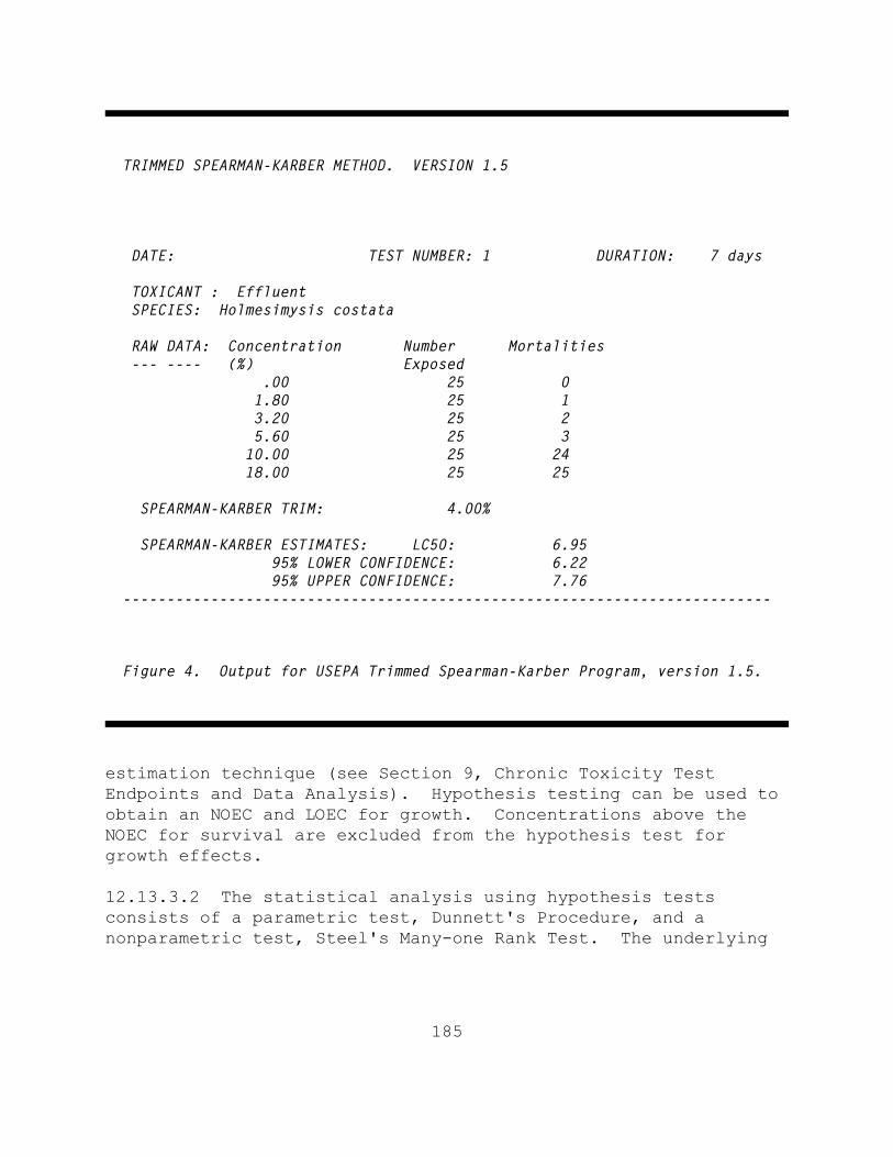
185

TRIMMED SPEARMAN-KARBER METHOD. VERSION 1.5

DATE: TEST NUMBER: 1 DURATION: 7 days

TOXICANT : Effluent SPECIES: Holmesimysis costata

RAW DATA: Concentration Number Mortalities --- ---- (%) Exposed .00 25 0 1.80 25 1 3.20 25 2 5.60 25 3 10.00 25 24 18.00 25 25

SPEARMAN-KARBER TRIM: 4.00%

SPEARMAN-KARBER ESTIMATES: LC50: 6.95 95% LOWER CONFIDENCE: 6.22 95% UPPER CONFIDENCE: 7.76--------------------------------------------------------------------------

Figure 4. Output for USEPA Trimmed Spearman-Karber Program, version 1.5.

estimation technique (see Section 9, Chronic Toxicity TestEndpoints and Data Analysis). Hypothesis testing can be used toobtain an NOEC and LOEC for growth. Concentrations above theNOEC for survival are excluded from the hypothesis test forgrowth effects.

12.13.3.2 The statistical analysis using hypothesis testsconsists of a parametric test, Dunnett's Procedure, and anonparametric test, Steel's Many-one Rank Test. The underlying

186

Figure 5. Flowchart for statistical analysis of mysid,Holmesimysis costata, growth data.

187

D ' 'ni'1(Xi & X)2

assumptions of the Dunnett's Procedure, normality and homogeneityof variance, are formally tested. The test for normality is theShapiro-Wilk's Test and Bartlett's Test is used to test forhomogeneity of variance. If either of these tests fails, thenonparametric test, Steel's Many-one Rank Test, is used todetermine the NOEC and LOEC endpoints. If the assumptions ofDunnett's Procedure are met, the endpoints are determined by theparametric test.

12.13.3.3 Additionally, if unequal numbers of replicates occuramong the concentration levels tested, there are parametric andnonparametric alternative analyses. The parametric analysis is at test with the Bonferroni adjustment. The Wilcoxon Rank SumTest with the Bonferroni adjustment is the nonparametricalternative. For detailed information on the Bonferroniadjustment, see Appendix D.

12.13.3.4 The data, mean and variance of the observations ateach concentration including the control for this example arelisted in Table 13. A plot of the data is provided in Figure 6. Since there is significant mortality in the 10.0% concentration,its effect on growth is not considered.

12.13.3.5 Test for Normality

12.13.3.5.1 The first step of the test for normality is tocenter the observations by subtracting the mean of allobservations within a concentration from each observation in thatconcentration. The centered observations are listed in Table 14.

12.13.3.5.2 Calculate the denominator, D, of the statistic:

188

TABLE 13. MYSID, HOLMESIMYSIS COSTATA, GROWTH DATA Concentration (%) Replicate Control 1.80 3.20 5.60 10.0 1 0.048 0.055 0.057 0.041 0.033 2 0.058 0.048 0.050 0.040 0.000 3 0.047 0.042 0.046 0.041 0.000 4 0.058 0.041 0.043 0.043 0.000 5 0.051 0.052 0.045 0.040 0.000

Mean(Yi) 0.052 0.048 0.048 0.041 0.007Si2 0.0000283 0.0000373 0.0000307 0.0000015 0.000218i 1 2 3 4 5

TABLE 14. CENTERED OBSERVATIONS FOR SHAPIRO-WILK'S EXAMPLE Concentration (%) Replicate Control 1.80 3.20 5.60 1 -0.004 0.007 0.009 0.000 2 0.006 0.000 0.002 -0.001 3 -0.005 -0.006 -0.002 0.000 4 0.006 -0.007 -0.005 0.002 5 -0.001 0.004 -0.003 -0.001

189

Figu

re 6

. Pl

ot o

f gr

owth

dat

a fo

r my

sid,

Hol

mesi

mysi

s co

stat

a, t

est.

190

TABLE 15. ORDERED CENTERED OBSERVATIONS FOR SHAPIRO-WILK'S EXAMPLE i X(i) i X(i) 1 -0.007 11 0.000 2 -0.006 12 0.000 3 -0.005 13 0.000 4 -0.005 14 0.002 5 -0.004 15 0.002 6 -0.003 16 0.004 7 -0.002 17 0.006 8 -0.001 18 0.006 9 -0.001 19 0.007 10 -0.001 20 0.009

Where: Xi = the ith centered observation X& = the overall mean of the centered observations n = the total number of centered observations

12.13.3.5.3 For this set of data, n = 20

X& = 1 (0.001) = 0.000 20

D = 0.000393

12.13.3.5.4 Order the centered observations from smallest tolargest

X(1) # X(2) # ... # X(n)

where X(i) denotes the ith ordered observation. The orderedobservations for this example are listed in Table 15.

191

W '1D[ 'ki'1ai(X

(n&i%1)&X (i))]2

TABLE 16. COEFFICIENTS AND DIFFERENCES FOR SHAPIRO-WILK'S EXAMPLE

i ai X(n-i+1) - X(i)

1 0.4734 0.016 X(20) - X(1) 2 0.3211 0.013 X(19) - X(2) 3 0.2565 0.011 X(18) - X(3) 4 0.2085 0.011 X(17) - X(4) 5 0.1686 0.008 X(16) - X(5) 6 0.1334 0.005 X(15) - X(6) 7 0.1013 0.004 X(14) - X(7) 8 0.0711 0.001 X(13) - X(8) 9 0.0422 0.001 X(12) - X(9) 10 0.0140 0.001 X(11) - X(10)

12.13.3.5.5 From Table 4, Appendix B, for the number ofobservations, n, obtain the coefficients a1, a2, ... ak where k isn/2 if n is even and (n-1)/2 if n is odd. For the data in thisexample, n = 20 and k = 10. The ai values are listed inTable 16.

12.13.3.5.6 Compute the test statistic, W, as follows:

The differences X(n-i+1) - X(i) are listed in Table 16. For this setof data: W = 1 (0.0194)2 = 0.958 0.000393

12.13.3.5.7 The decision rule for this test is to compare W ascalculated in Subsection 12.13.3.5.6 to a critical value found inTable 6, Appendix B. If the computed W is less than the criticalvalue, conclude that the data are not normally distributed. Forthis set of data, the critical value at a significance level of

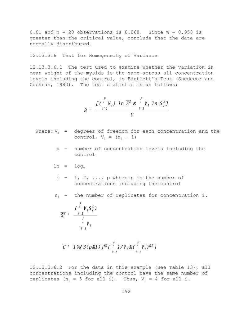
192

B '

[( 'Pi'1Vi) ln S2 & 'P

i'1Vi ln S 2

i]

C

0.01 and n = 20 observations is 0.868. Since W = 0.958 isgreater than the critical value, conclude that the data arenormally distributed.

12.13.3.6 Test for Homogeneity of Variance

12.13.3.6.1 The test used to examine whether the variation inmean weight of the mysids is the same across all concentrationlevels including the control, is Bartlett's Test (Snedecor andCochran, 1980). The test statistic is as follows:

Where: Vi = degrees of freedom for each concentration and thecontrol, Vi = (ni - 1)

p = number of concentration levels including thecontrol

ln = loge

i = 1, 2, ..., p where p is the number ofconcentrations including the control

ni = the number of replicates for concentration i.

S2 '

( 'Pi'1

ViS2i)

'Pi'1

Vi

C ' 1%[3(p&1)]&1[ 'Pi'11/Vi&( 'P

i'1Vi)

&1]

12.13.3.6.2 For the data in this example (See Table 13), allconcentrations including the control have the same number ofreplicates (ni = 5 for all i). Thus, Vi = 4 for all i.

193

B ' [(16)ln(0.0000245)&4 'Pi'1ln(S 2

i)]/1.104

TABLE 17. ANOVA TABLE Source df Sum of Squares Mean Square(MS) (SS) (SS/df)

2 Between p - 1 SSB SB = SSB/(p-1) 2 Within N - p SSW SW = SSW/(N-p)

12.13.3.6.3 Bartlett's statistic is therefore:

= [16(-10.617) - 4(-44.470)]/1.104 = [-169.872 - (-177.880)]/1.104 = 7.254

12.13.3.6.4 B is approximately distributed as chi-square with p- 1 degrees of freedom, when the variances are in fact the same. Therefore, the appropriate critical value for this test, at asignificance level of 0.01 with three degrees of freedom, is9.210. Since B = 7.254 is less than the critical value of 9.210,conclude that the variances are not different. 12.13.3.7 Dunnett's Procedure

12.13.3.7.1 To obtain an estimate of the pooled variance for theDunnett's Procedure, construct an ANOVA table as described inTable 17.

Where: p = number of concentration levels including the control

N = total number of observations n1 + n2 ... + np

194

ni = number of observations in concentration i

Between Sum of SquaresSSB ' 'Pi'1

T 2i/ni&G

2/N

Total Sum of SquaresSST ' 'Pi'1

'ni

j'1Y 2ij&G

2/N

Within Sum of Squares SSW ' SST&SSB

G = the grand total of all sample observations,

G ' 'Pi'1Ti

Ti = the total of the replicate measurements forconcentration i

Yij = the jth observation for concentration i(represents the mean weight of the mysids forconcentration i in test chamber j)

12.13.3.7.2 For the data in this example:

n1 = n2 = n3 = n4 = 5

N = 20

T1 = Y11 + Y12 + ... + Y15 = 0.262 T2 = Y21 + Y22 + ... + Y25 = 0.238 T3 = Y31 + Y32 + ... + Y35 = 0.241 T4 = Y41 + Y42 + ... + Y45 = 0.205 G = T1 + T2 + T3 + T4 = 0.946

SSB ' 'Pi'1T 2i/ni&G

2/N

= 1 (0.225) - (0.946)2 = 0.000254 5 20

SST ' 'Pi'1

'ni

j'1Y 2ij&G

2/N

= 0.0455 - (0.946)2 = 0.000754

195

TABLE 18. ANOVA TABLE FOR DUNNETT'S PROCEDURE EXAMPLE Source df Sum of Squares Mean Square (MS) (SS) (SS/df) Between 3 0.000254 0.0000847 Within 16 0.000500 0.0000313 Total 19 0.000754

ti '(Y1&Yi)

Sw (1/n1)%(1/ni)

20

SSW ' SST&SSB

= 0.000754 - 0.000254 = 0.000500

SB2 = SSB/(p-1) = 0.000254/(4-1) = 0.0000847

SW2 = SSW/(N-p) = 0.000500/(20-4) = 0.0000313

12.13.3.7.3 Summarize these calculations in the ANOVA table(Table 18).

12.13.3.7.4 To perform the individual comparisons, calculate thet statistic for each concentration, and control combination asfollows:

Where: Y&i = mean weight for concentration i Y&1 = mean weight for the control

SW = square root of the within mean square

n1 = number of replicates for the control

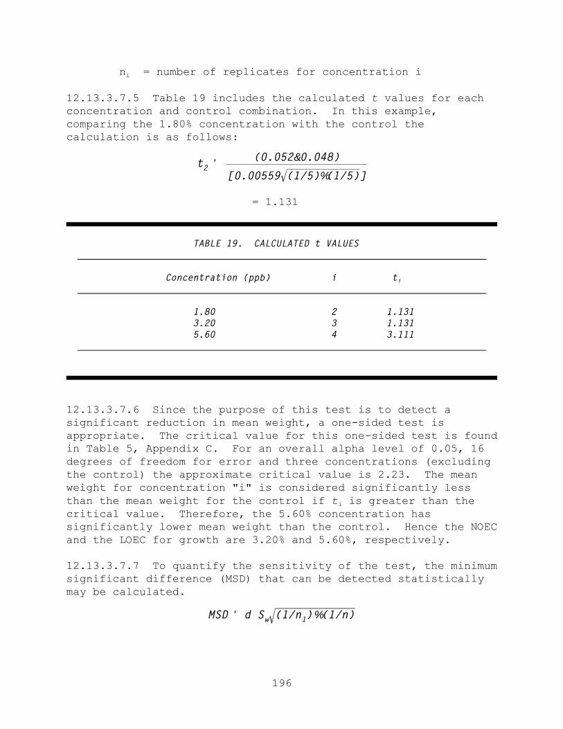
196

t2 '(0.052&0.048)

[0.00559 (1/5)%(1/5)]

TABLE 19. CALCULATED t VALUES

Concentration (ppb) i ti

1.80 2 1.131 3.20 3 1.131 5.60 4 3.111

MSD ' d Sw (1/n1)%(1/n)

ni = number of replicates for concentration i

12.13.3.7.5 Table 19 includes the calculated t values for eachconcentration and control combination. In this example,comparing the 1.80% concentration with the control thecalculation is as follows:

= 1.131

12.13.3.7.6 Since the purpose of this test is to detect asignificant reduction in mean weight, a one-sided test isappropriate. The critical value for this one-sided test is foundin Table 5, Appendix C. For an overall alpha level of 0.05, 16degrees of freedom for error and three concentrations (excludingthe control) the approximate critical value is 2.23. The meanweight for concentration "i" is considered significantly lessthan the mean weight for the control if ti is greater than thecritical value. Therefore, the 5.60% concentration hassignificantly lower mean weight than the control. Hence the NOECand the LOEC for growth are 3.20% and 5.60%, respectively.

12.13.3.7.7 To quantify the sensitivity of the test, the minimumsignificant difference (MSD) that can be detected statisticallymay be calculated.

197

MSD ' 2.23(0.00559) (1/5)%(1/5)

Where: d = the critical value for Dunnett's Procedure

SW = the square root of the within mean square

n = the common number of replicates at each concentration

(this assumes equal replication at each concentration)

n1 = the number of replicates in the control. 12.13.3.7.8 In this example:

= 2.23 (0.00559)(0.632)

= 0.00788

12.13.3.7.9 Therefore, for this set of data, the minimumdifference that can be detected as statistically significant is0.00788 mg.

12.13.3.7.10 This represents a 15.2% reduction in mean weightfrom the control.

12.13.3.8 Calculation of the ICp

12.13.3.8.1 The growth data from Table 13 are utilized in thisexample. As seen in the table, the observed means aremonotonically non-increasing with respect to concentration. Therefore, the smoothed means will be simply the correspondingobserved mean. The observed means are represented by Y&i and thesmoothed means by Mi. Table 20 contains the smoothed means andFigure 7 gives a plot of the smoothed response curve.

12.13.3.8.2 An IC25 can be estimated using the LinearInterpolation Method. A 25% reduction in weight, compared to thecontrols, would result in a mean weight of 0.039 mg, where M1(1-p/100) = 0.052(1-25/100). Examining the smoothed means and theirassociated concentrations (Table 20), the response, 0.039 mg, isbracketed by C4 = 5.60% and C5 = 10.0%.

198

ICp ' Cj%[M1(1&p/100)&Mj](C(j%1)&Cj)

(M(j%1)&Mj)

TABLE 20. MYSID, HOLMESIMYSIS COSTATA, MEAN GROWTH RESPONSE AFTER SMOOTHING S)))))))))))))))))))))))))))))))))))))))))))))))))))))))))))))))))Q

Toxicant Response Smoothed Conc. Means Means (%) i Yi (mg) Mi (mg) S)))))))))))))))))))))))))))))))))))))))))))))))))))))))))))))))))Q Control 1 0.052 0.052 1.80 2 0.048 0.048 3.20 3 0.048 0.048 5.60 4 0.041 0.041 10.00 5 0.0066 0.0066 18.00 6 0.000 0.000 S)))))))))))))))))))))))))))))))))))))))))))))))))))))))))))))))))Q

12.13.3.8.5 Using the equation in Section 4.2 from Appendix L,the estimate of the IC25 is calculated as follows:

IC25 = 5.60 + [0.052(1 - 25/100) - 0.041] (10.0 - 5.60) (0.0066 - 0.041) = 5.86%.

12.13.3.8.7 When the ICPIN program was used to analyze this setof data, requesting 80 resamples, the estimate of the IC25 was5.86%. The empirical 95.0% confidence interval for the true meanwas 4.9440% to 6.2553%. The computer program output for the IC25for this data set is shown in Figure 8.

12.14 PRECISION AND ACCURACY

12.12.1 PRECISION

12.12.1.1 Single-Laboratory Precision

12.12.1.1.1 Data on the single laboratory precision of theHolmesimysis costata growth and survival test with zinc sulfate

199

are shown in Table 21. NOECs for mysid survival were either 32or 56 µg/L Zn. There was also good agreement among LC50s, with acoefficient of variation of 14%. Mysids did not exhibit a growthresponse at zinc concentrations below those causing significantmortality; NOEC values for growth were always greater than orequal to the highest zinc concentration. IC50 values for growthcould not be calculated.

12.12.1.2 Multi-laboratory Precision

12.12.1.2.1 The multi-laboratory data indicate a similar levelof test precision (Table 22). The four multi-laboratory testswere conducted over a two year period, and each used spliteffluent samples tested at two laboratories. Survival NOECvalues were the same for both laboratories in three of the fourtests, with the NOECs varying by one concentration in the fourthtest. The mean coefficient of variation between LC50 values fromdifferent laboratories was 21%. The two available comparisons ofgrowth NOEC values indicate similar responses at bothlaboratories. Growth was the more sensitive indicator oftoxicity in three of the four effluent tests.

12.14.2 ACCURACY

12.14.2.1 The accuracy of toxicity tests cannot be determined.

200

Figu

re 7

. Pl

ot o

f ra

w da

ta,

obse

rved

mea

ns,

and

smoo

thed

mea

ns f

or t

he m

ysid

, Ho

lmes

imys

is c

osta

ta,

Grow

th d

ata

from

tab

les

13 a

nd 2

0

201

Conc. ID 1 2 3 4 5 6------------------------------------------------------------------------Conc. Tested 0 1.80 3.20 5.60 10.0 18.0------------------------------------------------------------------------Response 1 .048 .055 .057 .041 .033 0Response 2 .058 .048 .050 .040 0 0Response 3 .047 .042 .046 .041 0 0Response 4 .058 .041 .043 .043 0 0Response 5 .051 .052 .045 .040 0 0------------------------------------------------------------------------*** Inhibition Concentration Percentage Estimate ***Toxicant/Effluent: EffluentTest Start Date: Test Ending Date: Test Species: mysid, Holmesimysis costataTest Duration: 7 daysDATA FILE: mysid.icpOUTPUT FILE: mysid.i25-----------------------------------------------------------------------Conc. Number Concentration Response Std. Pooled ID Replicates % Means Dev. Response Means----------------------------------------------------------------------- 1 5 0.000 0.052 0.005 0.052 2 5 1.800 0.048 0.006 0.048 3 5 3.200 0.048 0.006 0.048 4 5 5.600 0.041 0.001 0.041 5 5 10.000 0.007 0.015 0.007 6 5 18.000 0.000 0.000 0.000-----------------------------------------------------------------------The Linear Interpolation Estimate: 5.8174 Entered P Value: 25-----------------------------------------------------------------------Number of Resamplings: 80The Bootstrap Estimates Mean: 5.8205 Standard Deviation: 0.2673Original Confidence Limits: Lower: 4.9440 Upper: 6.2553Expanded Confidence Limits: Lower: 4.5073 Upper: 6.4743Resampling time in Seconds: 0.22 Random_Seed: 526805435

Figure 8. Output for USEPA Linear Interpolation Program for the IC25.

202

TABLE 21. SINGLE LABORATORY PRECISION DATA FOR THE MYSID,HOLMESIMYSIS COSTATA GROWTH AND SURVIVAL TEST WITHZINC (ZN µG/L) SULFATE AS THE REFERENCE TOXICANT

Test SurvivalNOEC LC50

Growth NOEC

1 32 47 >32

2 32 59 >32

3 56 62 >56

4 56 65 >56

N 4 4 4

MeanSDCV (%)

44 58 7.914

>44

No growth effect was observed in zinc concentrations below thosecausing significant mortality (10, 18, 32, 56 and 100 µg/L).

All tests were conducted at MPSL.

203

TABLE 22. MULTI-LABORATORY PRECISION DATA FOR THE MYSID,HOLMESIMYSIS COSTATA GROWTH AND SURVIVAL TEST WITHSPLIT EFFLUENT (%) ON THE SAME DATE.

Test Effluent Type

Lab SurvivalNOEC LC50

GrowthNOEC

11

BKMEBKME

OSUMPSL

1.0 1.8 1.0 1.3

CV=26%

0.5L 0.5L

22

POTWPOTW

ATLMPSL

3.2 4.1 3.2 5.1

CV=14%

>3.2L>3.2L

33

POTWPOTW

SRHMPSL

10.0 12.810.0 11.7

CV=6%

na 3.2W

44

POTWPOTW

SRHMPSL

10.0 15.8 5.6 9.1

CV=38%

5.6W3.2W

Mean Interlaboratory CV= 21%

L Length was measured as the growth endpoint in tests 1 and 2,W Weight was measured in test 3 and 4.na Data was not available.

OSU is the Oregon State University Laboratory at the HatfieldMarine Science Center in Newport Oregon.

ATL is Aquatic Testing Laboratory in Ventura, California.

SRH is S.R. Hansen and Associates in Concord, California.

MPSL is the Marine Pollution Studies Laboratory near Monterey,California.

204

APPENDIX I. MYSID TEST: STEP-BY-STEP SUMMARY

PREPARATION OF TEST SOLUTIONS

A. Determine test concentrations and appropriate dilution waterbased on NPDES permit conditions and guidance from theappropriate regulatory agency.

B. Prepare effluent test solutions by diluting well mixedunfiltered effluent using volumetric flasks and pipettes. Use hypersaline brine where necessary to maintain all testsolutions at 34 ± 2‰. Include brine controls in tests thatuse brine.

C. Prepare a zinc reference toxicant stock solution (10,000µg/L) by adding 0.0440 g of zinc sulfate (ZnSO4N7H2O) to 1liter of reagent water.

D. Prepare zinc reference toxicant solution of 0 (control) 10,18, 32, 56 and 100 µg/L by adding 0, 1.0 1.8, 3.2, 5.6 and10.0 mL of stock solution, respectively, to a 1-L volumetricflask and filling to 1-L with dilution water.

E. Sample effluent and reference toxicant solutions forphysical/chemical analysis. Measure salinity, pH anddissolved oxygen from each test concentration.

F. Randomize numbers for test chambers and record the chambernumbers with their respective test concentrations on arandomization data sheet. Store the data sheet safely untilafter the test samples have been analyzed.

G. Place test chambers in a water bath or environmental chamberset to 13 or 15EC and allow temperature to equilibrate.

H. Measure the temperature daily in one random replicate (orseparate chamber) of each test concentration. Monitor thetemperature of the water bath or environmental chambercontinuously.

I. At the end of the test, measure salinity, pH, and dissolvedoxygen concentration from each test concentration.

205

PREPARATION AND ANALYSIS OF TEST ORGANISMS

A. Four to five days prior to the beginning of the toxicitytest, isolate approximately 150 gravid female mysids in ascreened (2-mm-mesh) compartment within an aerated 80-literaquarium (15EC). Add a surplus of Artemia nauplii (200 permysid, static; 500 per mysid, flow-through) to stimulateovernight release of juveniles. Add blades of kelp ashabitat.

B. Isolate the newly released juveniles by slowly siphoninginto a screen-tube (150-µm-mesh, 25 cm diam.) immersed in abucket of clean seawater. Transfer juveniles intoadditional screen-tubes or static 4-liter beakers at adensity of approximately 50 juveniles per liter. Juveniles should be fed five to ten newly released Artemianauplii per juvenile per day and a pinch (10 to 20 mg) ofground Tetramin® flake food per 100 juveniles per day.Maintain the juveniles for three days at 13 to 15EC,changing the water at least once in static chambers.

C. After three days, begin randomized introduction of juvenilesinto the test chambers. Place one or two mysids at a timeinto as many plastic cups as there are test chambers. Repeat the process until each cup has exactly five juvenilemysids.

D. Eliminate excess water from the cups (no more than 5 mLshould remain) and pipet the mysids into the test chambersusing a wide bore glass tube or pipet (approximately 3 mmID). Make sure no mysids are left in the randomizationcups. Count the number of juveniles in each test chamber toverify that each has five.

E. Remove all dead mysids daily, and add 40 newly hatchedArtemia nauplii/mysid/day, adjusting feeding to account formysid mortality.

F. At 48 and 96 hours, renew 75% of the test solution in eachchamber.

G. After 7 days, count and record the number of live and deadmysids in each chamber. After counting, use therandomization sheet to assign the correct test concentrationto each chamber. Remove all dead mysids.

206

H. Carefully pour the contents of each test chamber through asmall mesh screen (<300µm). Count the mysids and recordbefore screening. Briefly dip the screen containing themysids in fresh water to rinse away the salt. Carefullytransfer the mysids from the screen to a prenumbered,preweighed micro-weigh boat using fine-tipped forceps. Dryfor 24 hours at 60EC. Weigh each weigh boat on amicrobalance (accurate to 1 µg). Record the chamber number,mysid weight, weigh boat weight (recorded previously), andnumber of mysids per weigh boat (replicate) on the datasheet.

I. Analyze the data.

J. Include standard reference toxicant point estimate values inthe standard quality control charts.

207

Data Sheet for Juvenile Holmesimysis Toxicity Test

Test Start Date: Start Time: Mysid SourceTest End Date: End Time: Collection/Arrival Date:Reference Toxicant: Mysid Age at Start:Sample Source:

TestCont.

#ToxicConc.

Number Alive TotalNumber

Alive

TotalNumberat Start

Notes and Initials

Day 1 Day 2 Day 3 Day 4 Day 5 Day 6 Day 7

123456789

1011121314151617181920212223242526272829303132333435

Computer Data StorageDisk:File:

Note: See juvenile growth data on separate sheet.

208

Data Sheet for Weighing Juvenile Mysids Test Start Date:

Start Time:Mysid Source :

Test End Date:End Time:

Collection/Arrival Date:Reference Toxicant:

Mysid Age at Start:Sample Source:Sample Type:

TestContainerNumber

Site Codeor

Concentration

FoilNumber

FoilWeight

(µg)

TotalWeight

(µg)

Mysid Wt (Total - Foil)

(mg)

Number ofMysids

Weight perMysid(µg)

123456789

1011121314151617181920212223242526272829303132333435

Computer Data StorageDisk:File:Note: See mysid mortality data on separate sheet.

209

SECTION 13

PACIFIC OYSTER, Crassostrea gigasAND MUSSEL, Mytilus sp.

EMBRYO-LARVAL DEVELOPMENT TEST METHOD

Adapted from a method developed byGary A. Chapman, U.S. EPA, ORD Newport, ORand Debra L. Denton, U.S. EPA, Region IX

TABLE OF CONTENTS

13.1 Scope and Application 13.2 Summary of Method13.3 Interferences13.4 Safety13.5 Apparatus and Equipment13.6 Reagents and Supplies13.7 Effluents and Receiving Water Collection,

Preservation, and Storage13.8 Calibration and Standardization13.9 Quality Control13.10 Test Procedures13.11 Summary of Test Conditions and Test

Acceptability Criteria13.12 Acceptability of Test Results13.13 Data Analysis13.14 Precision and Accuracy

Appendix I Step-by Step Summary

210

SECTION 13

PACIFIC OYSTER, CRASSOSTREA GIGAS, AND MUSSEL, MYTILUS SPP.EMBRYO-LARVAL DEVELOPMENT TEST

13.1 SCOPE AND APPLICATION

13.1.1 This method estimates the chronic toxicity of effluentsand receiving waters to the embryos and larvae of several bivalvemolluscs, the Pacific oyster (Crassostrea gigas) and the mussels(Mytilus edulis, M. californianus, M. galloprovincialis, or M.trossulus) in a 48-h static non-renewal exposure. The effectsinclude the synergistic, antagonistic, and additive effects ofall the chemical, physical, and biological components whichadversely affect the physiological and biochemical functions ofthe test organisms.

13.1.2 Detection limits of the toxicity of an effluent orchemical substance are organism dependent.

13.1.3 Brief excursions in toxicity may not be detected using24-h composite samples. Also, because of the long samplecollection period involved in composite sampling, and because thetest chambers are not sealed, highly volatile and highlydegradable toxicants in the source may not be detected in thetest.

13.1.4 This test is commonly used in one of two forms: (1) adefinitive test, consisting of a minimum of five effluentconcentrations and a control, and (2) a receiving water test(s),consisting of one or more receiving water concentrations and acontrol.

13.1.5 This method should be restricted to use by, or under thesupervision of, professionals experienced in aquatic toxicitytesting. Specific experience with any toxicity test is usuallyneeded before acceptable results become routine.

13.2 SUMMARY OF METHOD

13.2.1 The method provides step-by-step instructions forperforming a 48-h static non-renewal toxicity test using embryosand larvae of the test species to determine the toxicity of

211

substances in marine and estuarine waters. The test endpoint isnormal shell development and should include mortality as ameasure of adverse effect.

13.3 INTERFERENCES

13.3.1 Toxic substances may be introduced by contaminants indilution water, glassware, sample hardware, and testing equipment(see Section 5, Facilities and Equipment, and Supplies).

13.3.2 Improper effluent sampling and handling may adverselyaffect test results (see Section 8, Effluent and Receiving WaterSampling, and Sample Handling, and Sample Preparation forToxicity Tests).

13.4 SAFETY

13.4.1 See Section 3, Health and Safety

13.5 APPARATUS AND EQUIPMENT

13.5.1 Tanks, trays, or aquaria -- for holding and acclimatingadult pacific oysters and mussels, e.g., standard salt wateraquarium or Instant Ocean Aquarium (capable of maintainingseawater at 10-20EC), with appropriate filtration and aerationsystem.

13.5.2 Air pump, air lines, and air stones -- for aerating watercontaining broodstock or for supplying air to test solutions withlow dissolved oxygen.

13.5.3 Constant temperature chambers or water baths -- formaintaining test solution temperature and keeping dilution watersupply, gametes, and embryo stock suspensions at test temperatureprior to the test.

13.5.4 Water purification system -- Millipore Super-Q, Deionizedwater (DI) or equivalent.

13.5.5 Refractometer -- for determining salinity.

13.5.6 Hydrometer(s) -- for calibrating refractometer.

212

13.5.7 Thermometers, glass or electronic, laboratory grade --for measuring water temperatures.

13.5.8 Thermometer, National Bureau of Standards Certified (seeUSEPA METHOD l70.l, USEPA, l979) -- to calibrate laboratorythermometers.

13.5.9 pH and DO meters -- for routine physical and chemicalmeasurements.

13.5.10 Standard or micro-Winkler apparatus -- for determiningDO (optional) and calibrating the DO meter.

13.5.11 Winkler bottles -- for dissolved oxygen determinations.

13.5.12 Balance -- Analytical, capable of accurately weighing to0.0001 g.

13.5.13 Fume hood -- to protect the analyst from effluent orformaldehyde fumes.

13.5.14 Glass stirring rods -- for mixing test solutions.

13.5.15 Graduated cylinders -- Class A, borosilicate glass ornon-toxic plastic labware, 50-l000 mL for making test solutions. (Note: not to be used interchangeably for gametes or embryos andtest solutions).

13.5.16 Volumetric flasks -- Class A, borosilicate glass or non-toxic plastic labware, 100-1000 mL for making test solutions.

13.5.17 Pipets, automatic -- adjustable, to cover a range ofdelivery volumes from 0.010 to 1.000 mL.

13.5.18 Pipet bulbs and fillers -- PROPIPET® or equivalent.

13.5.19 Wash bottles -- for reagent water, for topping offgraduated cylinders, for rinsing small glassware and instrumentelectrodes and probes.

13.5.20 Wash bottles -- for dilution water.

213

13.5.21 20-liter cubitainers or polycarbonate water cooler jugs-- for making hypersaline brine.

13.5.22 Cubitainers, beakers, or similar chambers of non-toxiccomposition for holding, mixing, and dispensing dilution waterand other general non-effluent, non-toxicant contact uses. Theseshould be clearly labeled and not used for other purposes.

13.5.23 Beakers, 50 mL -- for pooling surrogate water samplesfor chemistry measurements at the end of the test.

13.5.24 Beakers, 250 mL borosilicate glass -- for preparation oftest solutions.

13.5.25 Beakers, 1,000 mL borosilicate glass -- for mixinggametes for fertilization of eggs.

13.5.26 Inverted or compound microscope -- for inspectinggametes and making counts of embryos and larvae. The use of aninverted scope is not required, but recommended. Its use reducesthe exposure of workers to hazardous fumes (formalin orglutaraldehyde) during the counting of larvae and reduces sampleexamination time. Alternatively, a Sedgewick-Rafter cell may beused on a regular compound scope.

13.5.27 Counter, two unit, 0-999 -- for recording counts ofembryos and larvae.

13.5.28 A perforated plunger -- for maintaining a homogeneoussuspension of embryos.

13.5.29 Nytex screens, ca. 75 µm and ca. 37 µm -- for rinsinggametes to separate individual gametes from larger material; forretaining eggs, embryos, or larvae.

13.5.30 60 µm NITEX® filter -- for filtering receiving water.

13.6 REAGENTS AND SUPPLIES

13.6.1 Sample containers -- for sample shipment and storage (seeSection 8, Effluent and Receiving Water Sampling, and SampleHandling, and Sample Preparation for Toxicity Tests).

214

13.6.2 Data sheets (one set per test) -- for data recording (seeFigure 1).

13.6.3 Tape, colored -- for labelling test chambers andcontainers.

13.6.4 Markers, water-proof -- for marking containers, etc.

13.6.5 Parafilm -- to cover graduated cylinders and vesselscontaining gametes, embryos.

13.6.6 Gloves, disposable -- for personal protection fromcontamination.

13.6.7 Pipets, serological -- l-l0 mL, graduated.

13.6.8 Pipet tips -- for automatic pipets.

13.6.9 Coverslips -- for microscope slides.

13.6.10 Lens paper -- for cleaning microscope optics.

13.6.11 Laboratory tissue wipes -- for cleaning and dryingelectrodes, microscope slides, etc.

13.6.12 Disposable countertop covering -- for protection of worksurfaces and minimizing spills and contamination.

13.6.13 pH buffers 4, 7, and l0 (or as per instructions ofinstrument manufacturer) -- for standards and calibration check(see USEPA Method l50.l, USEPA, l979).

13.6.14 Membranes and filling solutions -- for dissolved oxygenprobe (see USEPA Method 360.l, USEPA, l979), or reagents formodified Winkler analysis.

13.6.15 Laboratory quality assurance samples and standards --for the above methods.

13.6.16 Test chambers -- 30 mL, four chambers per concentration. The chambers should be borosilicate glass or nontoxic disposable

215

plastic labware. The test may be performed in other sizedchambers as long as the density of embryos is the same.

13.6.17 Formaldehyde, 37% (Concentrated Formalin) -- forpreserving larvae. Note: formaldehyde has been identified as acarcinogen and is irritating to skin and mucous membranes. Itshould not be used at a concentration higher than necessary toachieve morphological preservation of larvae for counting andonly under conditions of maximal ventilation and minimalopportunity for volatilization into room air.

13.6.19 Reference toxicant solutions (see Section 13.10.2.4 andSection 4, Quality Assurance).

13.6.20 Reagent water -- defined as distilled or deionized waterthat does not contain substances which are toxic to the testorganisms (see Section 5, Facilities, Equipment, and Supplies andSection 7, Dilution Water).

13.6.21 Effluent and receiving water -- see Section 8, Effluentand Surface Water Sampling, and Sample Handling, and SamplePreparation for Toxicity Tests.

13.6.22 Dilution water and hypersaline brine -- see Section 7,Dilution Water and Section 13.6.24, Hypersaline Brines. Thedilution water should be uncontaminated 1-µm-filtered naturalseawater. Hypersaline brine should be prepared from dilutionwater.

13.6.23 HYPERSALINE BRINES

13.6.23.1 Most industrial and sewage treatment effluentsentering marine and estuarine systems have little measurablesalinity. Exposure of larvae to these effluents will usuallyrequire increasing the salinity of the test solutions. It isimportant to maintain an essentially constant salinity across alltreatments. In some applications it may be desirable to matchthe test salinity with that of the receiving water (See Section7.1). Two salt sources are available to adjust salinities --artificial sea salts and hypersaline brine (HSB) derived fromnatural seawater. Use of artificial sea salts is necessary onlywhen high effluent concentrations preclude salinity adjustment byHSB alone.

216

13.6.23.2 Hypersaline brine (HSB) can be made by concentratingnatural seawater by freezing or evaporation. HSB should be madefrom high quality, filtered seawater, and can be added to theeffluent or to reagent water to increase salinity. HSB hasseveral desirable characteristics for use in effluent toxicitytesting. Brine derived from natural seawater contains thenecessary trace metals, biogenic colloids, and some of themicrobial components necessary for adequate growth, survival,and/or reproduction of marine and estuarine organisms, and it canbe stored for prolonged periods without any apparent degradation. However, even if the maximum salinity HSB (100‰) is used as adiluent, the maximum concentration of effluent (0‰) that can betested is 66% effluent at 34‰ salinity (see Table 1).

13.6.23.3 High quality (and preferably high salinity) seawatershould be filtered to at least 10 µm before placing into thefreezer or the brine generator. Water should be collected on anincoming tide to minimize the possibility of contamination.

13.6.23.4 Freeze Preparation of Brine

13.6.23.4.1 A convenient container for making HSB by freezing isone that has a bottom drain. One liter of brine can be made fromfour liters of seawater. Brine may be collected by partiallyfreezing seawater at -10 to -20EC until the remaining liquid hasreached the target salinity. Freeze for approximately six hours,then separate the ice (composed mainly of fresh water) from theremaining liquid (which has now become hypersaline).

13.6.23.4.2 It is preferable to monitor the water until thetarget salinity is achieved rather than allowing total freezingfollowed by partial thawing. Brine salinity should never exceed 100‰. It is advisable not to exceed about 70‰ brine salinityunless it is necessary to test effluent concentrations greaterthan 50%.

13.6.23.4.3 After the required salinity is attained, the HSBshould be filtered through a 1 µm filter and poured directly intoportable containers (20-L cubitainers or polycarbonate watercooler jugs are suitable). The brine storage containers shouldbe capped and labelled with the salinity and the date the brinewas generated. Containers of HSB should be stored in the dark at

217

TABLE 1. MAXIMUM EFFLUENT CONCENTRATION (%) THAT CAN BE TESTED BY ADDING DILUTION WATERONLY OR BRINE ONLY (WITHOUT ADDITION OF DRY SEA SALTS), GIVEN VARIOUS EFFLUENTSALINITIES, DILUTION WATER SALINITIES, AND BRINE SALINITIES, AND MAINTAINING 30‰TEST SALINITY.

Effl. Dilution Water Salinity ‰ Brine Salinity ‰

‰ 31 32 33 34 35 60 70 80 90 100

0 3.23 6.25 9.09 11.76 14.29 50.00 57.14 62.50 66.67 70.00

1 3.33 6.45 9.38 12.12 14.71 50.85 57.97 63.29 67.42 70.71

2 3.45 6.67 9.68 12.50 15.15 51.72 58.82 64.10 68.18 71.43

3 3.57 6.90 10.00 12.90 15.63 52.63 59.70 64.94 68.97 72.16

4 3.70 7.14 10.34 13.33 16.13 53.57 60.61 65.79 69.77 72.92

5 3.85 7.41 10.71 13.79 16.67 54.55 61.54 66.67 70.59 73.68

10 4.76 9.09 13.04 16.67 20.00 60.00 66.67 71.43 75.00 77.78

15 6.25 11.76 16.67 21.05 25.00 66.67 72.73 76.92 80.00 82.35

20 9.09 16.67 23.08 28.57 33.33 75.00 80.00 83.33 85.71 87.50

25 16.67 28.57 37.50 44.44 50.00 85.71 88.89 90.91 92.31 93.33

218

4EC (even room temperature has been acceptable). HSB is usuallyof acceptable quality even after several months in storage.

13.6.23.5 Heat Preparation of Brine

13.6.23.5.1 The ideal container for making brine using heat-assisted evaporation of natural seawater is one that (1) has ahigh surface to volume ratio, (2) is made of a non-corrosivematerial, and (3) is easily cleaned (fiberglass containers areideal). Special care should be used to prevent any toxicmaterials from coming in contact with the seawater being used togenerate the brine. If a heater is immersed directly into theseawater, ensure that the heater materials do not corrode or leach any substances that would contaminate the brine. Onesuccessful method is to use a thermostatically controlled heatexchanger made from fiberglass. If aeration is needed, use onlyoil-free air compressors to prevent contamination. 13.6.23.5.2 Before adding seawater to the brine generator,thoroughly clean the generator, aeration supply tube, heater, andany other materials that will be in direct contact with thebrine. A good quality biodegradable detergent should be used,followed by several (at least three) thorough reagent waterrinses.

13.6.23.5.3 Seawater should be filtered to at least 10 µm beforebeing put into the brine generator. The temperature of theseawater is increased slowly to 40EC. The water should beaerated to prevent temperature stratification and to increasewater evaporation. The brine should be checked daily (dependingon the volume being generated) to ensure that the salinity doesnot exceed 100‰ an that the temperature does not exceed 40EC. Additional seawater may be added to the brine to obtain thevolume of brine required.

13.6.23.5.4 After the required salinity is attained, the HSBshould be filtered through a 1 µm filter and poured directly intoportable containers (20-L cubitainers or polycarbonate watercooler jugs are suitable). The brine storage containers shouldbe capped and labelled with the salinity and the date the brinewas generated. Containers of HSB should be stored in the dark at4EC (even room temperature has been acceptable). HSB is usuallyof acceptable quality even after several months in storage.

219

13.6.23.6 Artificial Sea Salts

13.6.23.6.1 No data from mussel or oyster tests using sea saltsor artificial seawater (e.g., GP2) are available for evaluationat this time, and their use must be considered provisional.

13.6.23.7 Dilution Water Preparation from Brine

13.6.23.7.1 Although salinity adjustment with brine is thepreferred method, the use of high salinity brines and/or reagentwater has sometimes been associated with discernible adverseeffects on test organisms. For this reason, it is recommendedthat only the minimum necessary volume of brine and reagent waterbe used to offset the low salinity of the effluent, and thatbrine controls be included in the test. The remaining dilutionwater should be natural seawater. Salinity may be adjusted inone of two ways. First, the salinity of the highest effluenttest concentration may be adjusted to an acceptable salinity, andthen serially diluted. Alternatively, each effluentconcentration can be prepared individually with appropriatevolumes of effluent and brine.

13.6.23.7.2 When HSB and reagent water are used, thoroughlymix together the reagent water and HSB before mixing in theeffluent. Divide the salinity of the HSB by the expected testsalinity to determine the proportion of reagent water to brine. For example, if the salinity of the brine is 100‰ and the test isto be conducted at 30‰, 100‰ divided by 30‰ = 3.33. Theproportion of brine is 1 part in 3.33 (one part brine to 2.33parts reagent water). To make 1 L of dilution water at 30‰salinity from a HSB of 100‰, 300 mL of brine and 700 mL ofreagent water are required. Verify the salinity of the resultingmixture using a refractometer.

13.6.23.8 Test Solution Salinity Adjustment

13.6.23.8.1 Table 2 illustrates the preparation of testsolutions (up to 50% effluent) at 34‰ by combining effluent, HSB,and dilution water. Note: if the highest effluent concentrationdoes not exceed 50% effluent, it is convenient to prepare brineso that the sum of the effluent salinity and brine salinityequals 68‰; the required brine volume is then always

220

equal to the effluent volume needed for each effluentconcentration as in the example in Table 2.

13.6.23.8.2 Check the pH of all test solutions and adjust towithin 0.2 units of dilution water pH by adding, dropwise, dilutehydrochloric acid or sodium hydroxide (see Section 8.8.9,Effluent and Receiving Water Sampling, Sample Handling, andSample Preparation for Toxicity Tests).

13.6.23.8.3 To calculate the amount of brine to add to eacheffluent dilution, determine the following quantities: salinityof the brine (SB, in ‰), the salinity of the effluent (SE, in ‰), and volume of the effluent to be added (VE, in mL). Then usethe following formula to calculate the volume of brine (VB, inmL) to be added:

VB = VE x (30 - SE)/(SB - 30)

13.6.23.8.4 This calculation assumes that dilution watersalinity is 30 ± 2‰.

13.6.23.9 Preparing Test Solutions

13.6.23.9.1 Ten mL of test solution are needed for each testcontainer. To prepare test solutions at low effluentconcentrations (<6%), effluents may be added directly to dilutionwater. For example, to prepare 1% effluent, add 1.0 mL ofeffluent to a 100-mL volumetric flask using a volumetric pipet orcalibrated automatic pipet. Fill the volumetric flask to the100-mL mark with dilution water, stopper it, and shake to mix. Pour into a (150-250 mL) beaker and stir. Distribute equalvolumes into the replicate test chambers. The remaining testsolution can be used for chemistry.

13.6.23.9.2 To prepare a test solution at higher effluentconcentrations, hypersaline brine must usually be used. Forexample, to prepare 40% effluent, add 400 mL of effluent to a 1-liter volumetric flask. Then, assuming an effluent salinity of2‰ and a brine salinity of 66‰, add 400 mL of brine (see equationabove and Table 2) and top off the flask with dilution water. Stopper the flask and shake well. Pour into a (100-250

221

TABLE 2. EXAMPLES OF EFFLUENT DILUTION SHOWING VOLUMES OFEFFLUENT (AT X‰), BRINE, AND DILUTION WATER NEEDED FORONE LITER OF EACH TEST SOLUTION.

FIRST STEP: Combine brine with reagent water or natural seawaterto achieve a brine of 68-x‰ and, unless natural seawater is usedfor dilution water, also a brine-based dilution water of 34‰.

SERIAL DILUTION:Step 1. Prepare the highest effluent concentration to be testedby adding equal volumes of effluent and brine to the appropriatevolume of dilution water. An example using 40% is shown.

Effluent Conc.(%)

Effluent x‰

Brine (68-x)‰

DilutionWater* 34‰

40 800 mL 800 mL 400 mL

Step 2. Make serial dilutions from the highest testconcentration.

Effluent Conc. (%) Effluent Source Dilution Water*(34‰)

20 1000 mL of 40% 1000 mL

10 1000 mL of 20% 1000 mL

5 1000 mL of 10% 1000 mL

2.5 1000 mL of 5% 1000 mL

Control none 1000 mL

INDIVIDUAL PREPARATION:

Effluent Conc.(%)

Effluent x‰ Brine (68-x)‰ DilutionWater* 34‰

40 400 mL 400 mL 200 mL

20 200 mL 200 mL 600 mL

10 100 mL 100 mL 800 mL

5 50 mL 50 mL 900 mL

2.5 25 mL 25 mL 950 mL

Control none none 1000 mL

*May be natural seawater or brine-reagent water equivalent.

222

mL) beaker and stir. Distribute equal volumes into the replicatetest chambers. The remaining test solution can be used forchemistry.

13.6.23.10 Brine Controls

13.6.23.10.1 Use brine controls in all tests where brine isused. Brine controls contain the same volume of brine as doesthe highest effluent concentration using brine, plus the volumeof reagent water needed to reproduce the hyposalinity of theeffluent in the highest concentration, plus dilution water. Calculate the amount of reagent water to add to brine controls byrearranging the above equation, (See, 13.6.23.8.3) setting SE =0, and solving for VE.

VE = VB x (SB - 30)/(30 - SE)

If effluent salinity is essentially 0‰, the reagent water volumeneeded in the brine control will equal the effluent volume at thehighest test concentration. However, as effluent salinity andeffluent concentration increase, less reagent water volume isneeded.

13.6.24 TEST ORGANISMS, OYSTERS AND MUSSELS

13.6.24.1 The test organisms for this test are the Pacific,oyster, Crassostrea gigas, or mussels, Mytilus spp. (at leasttwelve per test). Pacific oysters are native to Japan, but havebeen cultured commercially on the west coast of the United Statesfor over a century.

13.6.24.2 Species Identification

13.6.24.2.1 The three species of mussels included in this methodare presumably native to the west coast. The California mussel(Mytilus californianus) is distributed along the exposed rockycoast from Alaska to Baja California and is found from intertidalareas to 150 feet depth. The other two mussels included in thismethod (M. trossulus and M. galloprovinciallis) are common insheltered waters such as bays and estuaries and were previouslyconsidered to be west coast populations of Mytilus edulis. Thetwo species are both present in central California, with M.

223

galloprovincialis reported from San Francisco Bay to BajaCalifornia, and M. trossulus reported from Monterey to Alaska.

13.6.24.2.2 Test organisms should be identified to species usingmorphological features in recognized keys. Separation of the "M.edulis" complex, (M. trossulus, and M. galloprovinciallis) maynot be possible without electrophoretic characterization. Thegeographic source of the Mytilus spp. broodstock must bereported.

13.6.24.3 Obtaining Broodstock

13.6.24.3.1 Adult oysters (Crassostrea gigas) and mussels(Mytilus spp.) can be obtained from commercial suppliers and themussels can also be collected from the field. Organisms are bestshipped in damp towels or seaweed and kept cool (4-12EC). Note:if practical, check the sex ratio of brood stock or request suchinformation from a commercial supplier. A highly skewed sexratio could result in poor embryo yield.

13.6.24.4 Broodstock Culture and Handling

13.6.24.4.1 The adult bivalves are maintained in glass aquariaor fiberglass troughs or tanks. These are supplied continuously(approximately 5 L/min) with natural seawater, or salt waterprepared from commercial sea salts is recirculated. The animalsare checked daily and any obviously unhealthy animals arediscarded. Prior to spawning, the animals should be brushed orgently scraped to remove barnacles and other encrustingorganisms; this alleviates problems of egg and spermcontamination, especially through potential barnacle spawning.

13.6.24.4.2 Although ambient temperature seawater is usuallyacceptable for holding, recommended temperatures are 14-15EC foroyster and 8EC for mussels; conditioning bivalves to spawningcondition usually requires holding for from 1-8 weeks at a highertemperature (20EC for oysters, 15-18EC for mussels).

13.6.24.4.3 Natural seawater ($30‰) is used to maintain theadult animals and as a control water in the tests.

13.6.24.4.4 Adult animals used in field studies are transportedin insulated boxes or coolers packed with wet kelp or paper

224

toweling. Upon arrival at the field site, aquaria are filledwith control water, loosely covered with a styrofoam sheet andallowed to equilibrate to the holding temperature before animalsare added.

13.7 EFFLUENT AND RECEIVING WATER COLLECTION, PRESERVATION, AND STORAGE

13.7.1 See Section 8, Effluent and Receiving Water Sampling,Sample Handling, and Sample Preparation for Toxicity Tests.

13.8 CALIBRATION AND STANDARDIZATION

13.8.1 See Section 4, Quality Assurance.

13.9 QUALITY CONTROL

13.9.1 See Section 4, Quality Assurance.

13.10 TEST PROCEDURES

13.10.1 TEST DESIGN

13.10.1.1 The test consists of at least four replicates of fiveeffluent concentrations plus a dilution water control. Teststhat use brine to adjust salinity must also contain fourreplicates of a brine control. In addition, at least six extracount controls are prepared in dilution water and the number ofembryos in each are counted at the time of test initiation. These counts provide an average initial embryo density that isused in the calculation of test results (see 13.13.1.3). Extrareplicates are recommended for water chemistry during the tests(see Section 13.8 and Table 3).

13.10.1.2 Effluent concentrations are expressed as percenteffluent.

13.10.2 TEST SOLUTIONS

13.10.2.1 Receiving waters

13.10.2.1.1 The sampling point is determined by the objectivesof the test. At estuarine and marine sites, samples are usually

225

collected at mid-depth. Receiving water toxicity is determinedwith samples used directly as collected or with samples passedthrough a 60 µm NITEX® filter and compared without dilution,against a control. Using four replicate chambers per test, eachcontaining 10 mL, and 400 mL for chemical analysis, would requireapproximately 440 mL of sample per test.

13.10.2.2 Effluents

14.10.2.2.1 The selection of the effluent test concentrationsshould be based on the objectives of the study. A dilutionfactor of at least 0.5 is commonly used. A dilution factor of0.5 provides hypothesis test discrimination of ± 100%, andtesting of a 16 fold range of concentrations. Hypothesis testdiscrimination shows little improvement as dilution factors areincreased beyond 0.5 and declines rapidly if smaller dilutionfactors are used. USEPA recommends that one of the five effluenttreatments must be a concentration of effluent mixed withdilution water which corresponds to the permittee's instreamwaste concentration (IWC). At least two of the effluenttreatments must be of lesser effluent concentration than the IWC,with one being at least one-half the concentration of the IWC. If 100‰ HSB is used as a diluent, the maximum concentration ofeffluent that can be tested will be 70% at 30‰ salinity.

13.10.2.2.2 If the effluent is known or suspected to be highlytoxic, a lower range of effluent concentrations should be used(such as 25%, 12.5%, 6.25%, 3.12% and 1.56%).

13.10.2.2.3 The volume in each test chamber is 10 mL.

13.10.2.2.4 Effluent dilutions should be prepared for allreplicates in each treatment in one container to minimizevariability among the replicates. Dispense into the appropriateeffluent test chambers.

13.10.2.3 Dilution Water

13.10.2.3.1 Dilution water should be uncontaminated 1-µm-filtered natural seawater or hypersaline brine (prepared fromuncontaminated natural seawater) plus reagent water (see Section

226

7, Dilution Water). Natural seawater may be uncontaminatedreceiving water. This water is used in all dilution steps and asthe control water.

13.10.2.4 Reference Toxicant Test

13.10.2.4.1 Reference toxicant tests should be conducted asdescribed in Quality Assurance (see Section 4.7).

13.10.2.4.2 The preferred reference toxicant for oysters andmussels is copper chloride (CuCl2NH2O). Reference toxicant testsprovide an indication of the sensitivity of the test organismsand the suitability of the testing laboratory (see Section 4Quality Assurance). Another toxicant may be specified by theappropriate regulatory agency. Prepare a copper referencetoxicant stock solution (2,000 mg/L) by adding 5.366 g of copperchloride (CuCl2N2H2O) to 1 liter of reagent water. For eachreference toxicant test prepare a copper sub-stock of 3 mg/L bydiluting 1.5 mL of stock to one liter with reagent water. Alternatively, certified standard solutions can be ordered fromcommercial companies.

13.10.2.4.3 Prepare a control (0 Fg/L) plus four replicates eachof at least five consecutive copper reference toxicant solutions(e.g., from the series 3.0, 4.4, 6.5, 9.5, 13.9, 20.4, and 30.0Fg/L, by adding 0.10, 0.15, 0.22, 0.32, 0.46, 0.68, and 1.00 mLof sub-stock solution, respectively, to 100-mL volumetric flasksand filling to 100-mL with dilution water). Start with controlsolutions and progress to the highest concentration to minimizecontamination.

13.10.2.4.4 If the effluent and reference toxicant tests are tobe run concurrently, then the tests must use embryos from thesame spawn. The tests must be handled in the same way and testsolutions delivered to the test chambers at the same time. Reference toxicant tests must be conducted at 30 ± 2‰.

13.10.3 COLLECTION OF GAMETES FOR THE TEST

13.10.3.1 Spawning Induction

13.10.3.1.1 Select at least a dozen bivalves and place them intoa container filled with seawater (ca. 20EC for oysters, 15EC for

227

mussels) and allow time for them to resume pumping (ca. 30minutes). Mussels will often start pumping following immersionif they have been kept out of water and refrigerated overnightprior to spawning.

TABLE 3. EXAMPLE OF TYPICAL TEST ARRAY SHOWING NUMBER AND TYPESOF TREATMENT CHAMBERS REQUIRED.

TREATMENT Test Vials ChemistryVials

Count Control 6 0

Brine Control 4 1-3

Dilution Water Control 4 1-3

Effluent conc. 1 4 1-3

Effluent conc. 2 4 1-3

Effluent conc. 3 4 1-3

Effluent conc. 4 4 1-3

Effluent conc. 5 4 1-3

TOTAL Chambers = 41-55 34 7-21

13.10.3.1.2 Over a 15-20 minute period, increase the temperature(do not exceed 32EC for oysters, or 20EC for mussels), checkingfor spawning.

13.10.3.1.3 If no spawning occurs after 30 minutes, replace thewater with some at the original temperature and after 15 minutesagain increase the temperature as in 13.10.3.2. Although ASTM(1993) cautions against it, the addition of algae into the watercan often stimulate spawning of bivalves; if this method is used,the organisms should be moved to clean water once spawningbegins. Mussels can also be induced to spawn by injection of 0.5M KCl into the posterior adductor muscle. Oysters can be inducedto spawn by the addition of heat-killed sperm about one hourafter initial temperature increase.

13.10.3.2 Pooling Gametes

228

13.10.3.2.1 When individuals are observed to be sheddinggametes, remove each spawner from the tank and place each in aseparate container (20EC water for oysters, 15EC for mussels). Alternatively, bivalves can be placed into individual chambersinitially (at temperatures per 13.10.5.2) and these placed into awater bath that provides the desired maximum temperature.

13.10.3.2.2 Early in the spawning process, examine a smallsample of the gametes from each spawner to confirm sex and to seeif the gametes are of adequate quality.

13.10.3.2.3 Place a small amount of sperm from each male onto amicroscope slide (well slides work nicely). Examine the spermfor motility; use sperm from those males with the better spermmotility.

13.10.3.2.4 A small sample of the eggs from each female shouldbe examined for the presence of significant quantities of pooreggs (vacuolated, small, or abnormally shaped). If good qualityeggs are available from one or more females, questionable batchesof eggs should not be used for the test. It is more important touse high quality eggs than it is to use a pooled population ofeggs.

13.10.3.2.5 Sperm and egg suspensions that are to be used forpreparing the embryo stock should be passed through Nytex screen(ca. 75 Fm) to separate out clumps of gametes or extraneousmaterial.

13.10.3.2.6 The pooled eggs are placed into a 1 L beaker andsufficient dilution water added to achieve an egg density ofabout 5,000-8,000 eggs/mL (objects are just discernible whenviewed through the egg suspension) in about 800-900 mL watervolume.

13.10.3.3 Fertilization

13.10.3.3.1 Sperm density may vary from one spawning to thenext. It is important to use enough sperm to achieve a highpercent egg fertilization, but too many sperm can causepolyspermy with resultant abnormal development. To achieve anacceptable level of sperm, several egg suspensions of equaldensity should be fertilized using a range of sperm volumes,

229

e.g., 100 mL of egg suspension plus 1, 3, and 10 mL of spermsuspension. This test fertilization should be accomplishedwithin 1 hour of spawning. Use the eggs with the lowest amountof sperm giving normal embryo development after 1.5-2.5 hoursafter fertilization, as determined by microscopic examination. Usually >90% of the eggs should be fertilized; oysters shouldhave changed from the tear-drop shaped egg to a round single cellzygote; mussels should show a single polar body; or embryos ofeither species should have advanced to the two-cell stage.

13.10.4 START OF THE TEST

13.10.4.1 Prior to Beginning the Test

13.10.4.1.1 The test should begin as soon as possible,preferably within 24 h of sample collection. The maximum holdingtime following retrieval of the sample from the sampling deviceshould not exceed 36 h for off-site toxicity tests unlesspermission is granted by the permitting authority. In no caseshould the sample be used in a test more than 72 h after samplecollection (see Section 8 Effluent and Receiving Water Sampling,Sample Handling, and Sample Preparation for Toxicity Test).

13.10.4.1.2 Just prior to test initiation (approximately 1 h),the temperature of a sufficient quantity of the sample to makethe test solutions should be adjusted to the test temperature (18or 20 ± 1EC) and maintained at that temperature during theaddition of dilution water.

13.10.4.1.3 Increase the temperature of the water bath, room, orincubator to the required test temperature (18 or 20 ± 1EC).

13.10.4.1.4 Randomize the placement of test chambers in thetemperature-controlled water bath, room, or incubator at thebeginning of the test, using a position chart. Assign numbersfor the position of each test chamber using a random numbers orsimilar process (see Appendix A, for an example ofrandomization). Maintain the chambers in this configurationthroughout the test, using a position chart. Record thesenumbers on a separate data sheet together with the concentrationand replicate numbers to which they correspond. Identify thissheet with the date, test organism, test number, laboratory, and

230

investigator's name, and safely store it away until after theoysters or mussels have been examined at the end of the test.

13.10.4.1.5 Note: Loss of the randomization sheet wouldinvalidate the test by making it impossible to analyze the dataafterwards. Make a copy of the randomization sheet and storeseparately. Take care to follow the numbering system exactlywhile filling chambers with the test solutions.

13.10.4.1.6 Arrange the test chambers randomly in the water bathor controlled temperature room. Once chambers have been labeledrandomly, they can be arranged in numerical order forconvenience, since this will also ensure random placement oftreatments.

13.10.4.2 Estimation of Embryo Density

13.10.4.2.1 Adjust the embryo suspension to a density of 1,500-3,000/mL. Confirm by counting chamber counts on 1 mL subsamplesfrom a stirred suspension of embryos. Final larval density of15/mL will provide reasonable precision (150 larvae) and beeasier to count than 300 larvae. Add 0.1 mL of the embryosuspension to 10 mL of test solution into each of the randomizedtest vials. It is extremely important (for a consistent embryodensity among test chambers) to maintain a homogeneousdistribution of embryos in the stock suspension by regular, slowoscillation of a perforated plunger during embryo distribution.

13.10.4.3 Initial Density Counts

13.10.4.3.1 If tests are conducted on small volumes, using aninverted microscope, the total number of embryos injected intothe count controls should be determined as soon as the test hasbeen started. If larger test volumes are used, with counts basedupon subsamples, the embros should be resuspended in the waterusing a perforated plunger. Then subsamples are taken (e.g., 5-10 mL) and the total number of embryos counted in the subsample. Two methods for these counts are to use a counting chamber of thesame volume as the subsample, or to screen the embryos using a 37Fm screen and backwash with a smaller volume for small countingchambers. In either procedure, appropriate multiple rinsing isneeded to achieve quantitative transfer of embryos.

231

13.10.4.3.2 Initial counts are required to determine survival inthe controls and other treatments. High coefficients ofvariability in initial counts make survival estimates inexact andmay actually decrease the sensitivity of the test.

13.10.4.4 Incubation

13.10.4.4.1 Cover and incubate the chambers in an environmentalchamber or by partial immersion in a temperature-controlled waterbath for 48 hours.

13.10.4.4.2 At the end of the 48-hour incubation period, examinea count control test chamber (or control test vial if the countcontrols were transferred to a counting chamber to make theinitial counts) under a microscope to check for completedevelopment of control organisms. If development is complete,the test should be ended. If development does not appear to becomplete, the test should be continued until complete developmentoccurs (but not beyond 54 hours total test duration).

13.10.5 LIGHT, PHOTOPERIOD, SALINITY AND TEMPERATURE

13.10.5.1 The light quality and intensity should be at ambientlaboratory conditions. Light intensity should be 10-20 µE/m2/s,or 50 to 100 foot candles (ft-c), with a 16 h light and 8 h darkcycle.

13.10.5.2 The water temperature in the test chambers should bemaintained at 18 or 20 ± 1EC. If a water bath is used tomaintain the test temperature, the water depth surrounding thetest cups should be as deep as possible without floating thechambers.

13.10.5.3 The test salinity should be in the range of 30 ± 2‰. The salinity should vary by no more than ±2‰ among the chamberson a given day. If effluent and receiving water tests areconducted concurrently, the salinities of these tests should besimilar.

13.10.5.4 Rooms or incubators with high volume ventilationshould be used with caution because the volatilization of thetest solutions and evaporation of dilution water may cause widefluctuations in salinity. Covering the test chambers with clean

232

polyethylene plastic may help prevent volatilization andevaporation of the test solutions.

13.10.6 DISSOLVED OXYGEN (DO) CONCENTRATION

13.10.6.1 Aeration may affect the toxicity of effluent andshould be used only as a last resort to maintain a satisfactoryDO. The DO concentration should be measured on new solutions atthe start of the test (Day 0). The DO should not fall below 4.0mg/L (see Section 8, Effluent and Receiving Water Sampling,Sample Handling, and Sample Preparation for Toxicity Tests). Ifit is necessary to aerate, all treatments and the control shouldbe aerated. The aeration rate should not exceed that necessaryto maintain a minimum acceptable DO and under no circumstancesshould it exceed 100 bubbles/minute, using a pipet with a 1-2 mmorifice, such as a 1 mL KIMAX® serological pipet No. 37033, orequivalent.

13.10.7 OBSERVATIONS DURING THE TEST

13.10.7.1 Routine Chemical and Physical Observations

13.10.7.1.1 DO is measured at the beginning of the exposureperiod in each test concentration and in the control.

13.10.7.1.2 Temperature, pH, and salinity are measured at thebeginning of the exposure period in each test concentration andin the control. Temperature should also be monitored continuouslyor observed and recorded daily for at least two locations in theenvironmental control system or the samples. Temperature shouldbe measured in a sufficient number of test chambers at the end ofthe test to determine temperature variation in the environmentalchamber.

13.10.7.1.3 Record all the measurements on the data sheet.

13.10.8 TERMINATION OF THE TEST

13.10.8.1 Ending the Test

13.10.8.1.1 Record the time the test is terminated.

13.10.8.1.2 The pH, dissolved oxygen, and salinity are measured

233

at the end of the exposure period in one test chamber at eachconcentration and in the control. If small electrodes are used,these measurements can be performed in a single extra replicate vial set up specifically for this measurement. Measurementsshould not be made in vials that are to be counted, as larvae mayadhere to electrodes, possibly biasing larval counts.

13.10.8.2 Sample Preservation

13.10.8.2.1 To terminate the test, add 0.25 mL of concentratedformalin (37% formaldehyde). It is advisable not to shake thecontents at any time following test termination because thelarvae may stick to the edge of the chambers. Simply allow thepreservative to mix passively and the larvae to settle out. Theuse of glutaraldehyde instead of formalin is likely to beacceptable, but as no record of its use with this test is known,care should be taken to confirm that glutaraldehyde kills,preserves, and produces no artifacts that would confound the testresults.

13.10.8.2.2 Note: Formaldehyde has been identified as acarcinogen and both glutaraldehyde and formaldehyde areirritating to skin and mucus membranes. Neither should be usedat higher concentrations than needed to achieve morphologicalpreservation and only under conditions of maximal ventilation andminimal opportunity for volatilization into room air.

13.10.8.3 Counting

13.10.8.3.1 After addition of preservative, observe all thelarvae in each test vial. This can be done by examining thecontents of each test vial with an inverted microscope at about40X-50X magnification or by quantitative transfer of all larvaeonto a counting chamber and counting using a compound microscopeat about 100X. Using the mechanical stage, carefully count andscore all larvae as either normal or abnormal. If substantialnumbers of completely developed shells without meat are observed(i.e., > 5 percent of normal larvae), then these shells should beenumerated separately (as dead larvae). "Larvae possessingmisshapened or otherwise malformed shells are considered normal,provided development has been completed" (ASTM, 1994). Recordthe final counts on the data sheet.

234

13.10.8.3.2 If the number of larvae observed appears to be lowin relation to the number inoculated at the beginning of thetest, this signifies either mortality and dissolution, orpossible adherence to the walls of the vials or incompletetransfer to the counting chamber. Inspect the vials for evidenceof the latter two occurrences.

13.10.8.4 Endpoint

13.10.8.4.1 The percentage of embryos that did not survive anddevelop to live larvae with completely developed shells (i.e.,abnormal or dead organisms) is calculated for each treatmentreplicate (See 13.13.1.3). All larvae are considered live unlessthey are merely empty shells "without meat" (ASTM, 1994); embryosand larvae that are not yet in the D-hinge stage are counted asabnormal, even if they may have died during the test. Embryosand larvae that die and disintegrate during the test areestimated from initial embryo counts (See N' in 13.13.1.3).

13.10.8.4.2 Unless used as the dilution water, natural seawatercontrols are only used to check the relative performance of thedilution water controls (e.g., brine controls) required forsalinity adjustment. Statistical analysis should use theappropriate dilution water control data.

13.11 SUMMARY OF TEST CONDITIONS AND TEST ACCEPTABILITY CRITERIA

13.11.1 A summary of test conditions and test acceptabilitycriteria is listed in Table 4.

TABLE 4. SUMMARY OF TEST CONDITIONS AND TEST ACCEPTABILITYCRITERIA FOR, CRASSOSTREA GIGAS and MYTILUS SPP.,EMBRYO-LARVAL DEVELOPMENT TEST WITH EFFLUENTS ANDRECEIVING WATERS

1. Test type: Static non-renewal

2. Salinity: 30 ± 2‰

3. Temperature: 20 ± 1EC (oysters)15 or 18 ± 1EC (mussels)*

4. Light quality: Ambient laboratory light

235

5. Light intensity: l0-20 uE/m2/s (Ambientlaboratory levels)

6. Photoperiod: 16 h light, 8 h darkness

7. Test chamber size: 30 mL

8. Test solution volume: 10 mL

9. No. larvae per chamber: 150-300

10. No. replicate chambersper concentration:

4 (plus 3 chemistry vials)

11. Dilution water: Uncontaminated 1-µm-filterednatural seawater or hypersalinebrine prepared from naturalseawater

12. Test concentrations: Effluents: Minimum of 5 and acontrolReceiving waters: 100%receiving water and a control

13. Dilution factor: Effluents: $0.5Receiving waters: None or $0.5

14. Test duration: 48 hours (or until completedevelopment up to 54 hours)

15. Endpoint: Survival and normal shelldevelopment

16. Test acceptability criteria:

Control survival must be $70%for oyster embryos or $50% formussel embryos in controlvials; $90% normal shelldevelopment in survivingcontrols; and must achieve a%MSD of <25%

236

17. Sampling requirements: One sample collected at testinitiation, and preferably usedwithin 24 h of the time it isremoved from the samplingdevice (see Section 8, Effluentand Receiving Water Sampling,Sample Handling, and SamplePreparation for Toxicity Tests)

18. Sample volume required: 1 L per test

*Mussel embryo-larval tests were commonly conducted at 15EC(ASTM, 1994). Experience has shown that many laboratories innorthern Californa, Oregon, and Washington often fail to achieveadequate control development at 15EC in 48 hours. It isacceptable to conduct the test at 15EC with the permission of theregulatory authority. Developmental rates may be dependent uponspecies, local population characteristics, or other factors.

13.12 ACCEPTABILITY OF TEST RESULTS

13.12.1 For tests to be considered acceptable, the followingrequirements must be met:

(1) The mean survival must be at least 70% for oysters orat least 50% for mussels in the controls.

(2) The percent normal must be at least 90% in thesurviving controls.

(3) The minimum significant difference (%MSD) is <25%relative to the control.

13.13 DATA ANALYSIS

13.13.1 GENERAL

13.13.1.1 Tabulate and summarize the data. Calculate theproportion of normally developed larvae for each replicate. Asample set of test data is listed in Table 5.

237

13.13.1.2 Final calculations are based upon counts of normallarvae and total larvae at test termination, and mean initialembryo count.

13.13.1.3 The percentage of embryos that did not survive ordevelop to live larvae with completely developed shells (i.e.,abnormal or dead organisms) is calculated for each treatmentreplicate (including controls) using the formula:

A = 100 (N' - B') N'

where:

A = percent abnormal and dead organismsB' = the adjusted number of normal larvae at the end of the testN' = the initial number of embryos in the test chambers expressed as the mean of the initial counts;

and: if N > N', where

N = the actual number of larvae at the end of the testthen: B' = B (N' / N)

where: B = the actual number of normal larvae at the end of the test but, when N # N', then: B' = B

The means of "A" are obtained for each treatment concentration,and the latter are corrected for control response using Abbott'sformula, as follows:

E = 100 (A - M) 100 - M

where:

E = the mean percent abnormal/dead corrected for controlsA = the mean percent abnormal/deadM = the value of A for the controls.

13.13.1.4 The statistical tests described here must be used witha knowledge of the assumptions upon which the tests arecontingent. The assistance of a statistician is recommended foranalysts who are not proficient in statistics.

238

TABLE 5. DATA FROM BIVALVE DEVELOPMENT TEST)))))))))))))))))))))))))))))))))))))))))))))))))))))))))))))CopperConcentration Initial Number Number Proportion(µg/L) Replicate Density Surviving Normal Normal ))))))))))))))))))))))))))))))))))))))))))))))))))))))))))))))))))))))))) Control A 25 22 22 1.00 B 25 25 24 0.96 C 25 25 25 1.00 D 30 30 29 0.97 0.13 A 25 23 22 0.96 B 30 30 29 0.97 C 25 25 25 1.00 D 25 24 23 0.96 0.25 A 25 25 23 0.92 B 25 19 18 0.95 C 25 21 19 0.90 D 25 23 22 0.96 0.50 A 25 11 10 0.91 B 25 14 13 0.93 C 25 17 15 0.88 D 25 15 14 0.93 1.00 A 25 8 7 0.88 B 25 6 5 0.83 C 25 8 7 0.88 D 25 11 9 0.82 2.00 A 25 2 2 1.00 B 25 3 2 0.67 C 25 4 3 0.75 D 25 5 2 0.40

13.13.1.5 The endpoints of toxicity tests using bivalves arebased on the reduction in proportion of normally developedlarvae. The IC25 is calculated using the Linear InterpolationMethod (see Section 9, Chronic Toxicity Test Endpoints and DataAnalysis). LOEC and NOEC values for larval development areobtained using a hypothesis testing approach such as Dunnett'sProcedure (Dunnett, 1955) or Steel's Many-one Rank Test (Steel,1959; Miller, 1981) (see Section 9). Separate analyses areperformed for the estimation of the LOEC and NOEC endpoints andfor the estimation of the IC25. See the Appendices for examplesof the manual computations, and examples of data input andprogram output.

13.13.2 EXAMPLE OF ANALYSIS OF BIVALVE EMBRYO-LARVALDEVELOPMENT DATA

239

13.13.2.1 Formal statistical analysis of the embryo-larvaldevelopment is outlined in Figure 1. The response used in theanalysis is the proportion of normally developed surviving larvaein each test or control chamber. Separate analyses are performedfor the estimation of the NOEC and LOEC endpoints and for theestimation of the IC25 endpoint. Concentrations at which thereis no normal development in any of the test chambers are excludedfrom statistical analysis of the NOEC and LOEC, but included inthe estimation of the IC25.

13.13.2.2 For the case of equal numbers of replicates across allconcentrations and the control, the evaluation of the NOEC andLOEC endpoints is made via a parametric test, Dunnett'sProcedure, or a nonparametric test, Steel's Many-one Rank Test,on the arc sine square root transformed data. Underlyingassumptions of Dunnett's Procedure, normality and homogeneity ofvariance, are formally tested. The test for normality is theShapiro-Wilk's Test, and Bartlett's Test is used to test forhomogeneity of variance. If either of these tests fails, thenonparametric test, Steel's Many-one Rank Test, is used todetermine the NOEC and LOEC endpoints. If the assumptions ofDunnett's Procedure are met, the endpoints are estimated by theparametric procedure.

13.13.2.3 If unequal numbers of replicates occur among theconcentration levels tested, there are parametric andnonparametric alternative analyses. The parametric analysis is at test with the Bonferroni adjustment (see Appendix D). TheWilcoxon Rank Sum Test with the Bonferroni adjustment is thenonparametric alternative.

13.13.2.4 Example of Analysis of Embryo-Larval Development Data

13.13.2.4.1 Since the response of interest is the proportion ofnormally developed surviving larvae, each replicate must first betransformed by the arc sine square root transformation proceduredescribed in Appendix B. Because there are varying numbers ofsurvivors in the replicates, the adjustment for responseproportions of zero or one will not be made. The raw andtransformed data, means and variances of the transformedobservations at each effluent concentration and control arelisted in Table 5. The data are plotted in Figure 2.

240

Figure 1. Flowchart for statistical analysis of the pacific oyster, Crassostrea gigas, andmussel, Mytilus spp., development data.

241

TABLE 6. BIVALVE EMBRYO-LARVAL DEVELOPMENT DATAS)))))))))))))))))))))))))))))))))))))))))))))))))))))))))))) Copper Concentration (µg/L) ))))))))))))))))))))))))))))))))))))))))))) Replicate Control 0.13 0.25 0.50 1.00 2.00S))))))))))))))))))))))))))))))))))))))))))))))))))))))))))))))))))))))))) A 1.00 0.96 0.92 0.91 0.88 1.00RAW B 0.96 0.97 0.95 0.93 0.83 0.67 C 1.00 1.00 0.90 0.88 0.88 0.75 D 0.97 0.96 0.96 0.93 0.82 0.40S)))))))))))))))))))))))))))))))))))))))))))))))))))))))))))))))))))))))))ARC SINE A 1.571 1.369 1.284 1.266 1.217 1.571SQUARE ROOT B 1.369 1.397 1.345 1.303 1.146 0.959TRANSFORMED C 1.571 1.571 1.249 1.217 1.217 1.047 D 1.397 1.369 1.369 1.303 1.133 0.685S)))))))))))))))))))))))))))))))))))))))))))))))))))))))))))))))))))))))))Mean (Y&i) 1.477 1.427 1.312 1.272 1.178 1.066Si2 0.01191 0.00945 0.00303 0.00166 0.00203 0.13733

i 1 2 3 4 5 6S)))))))))))))))))))))))))))))))))))))))))))))))))))))))))))))))))))))))))

D ' 'ni'1

(Xi & X )2

13.13.2.5 Test for Normality

13.13.2.5.1 The first step of the test for normality is tocenter the observations by subtracting the mean of allobservations within a concentration from each observation in thatconcentration. The centered observations are summarized inTable 6.

13.13.2.5.2 Calculate the denominator, D, of the statistic:

Where: Xi = the ith centered observation X& = the overall mean of the centered observations n = the total number of centered observations

13.13.2.5.3 For this set of data, n = 24

X& = 1 (-0.002) = 0.000 24

D = 0.4963

242

TABLE 7. ORDERED CENTERED OBSERVATIONS FOR SHAPIRO-WILK'S EXAMPLE

))))))))))))))))))))))))))))))))))))))))))))))))))))))))))))) i X(i) i X(i)))))))))))))))))))))))))))))))))))))))))))))))))))))))))))))) 1 -0.381 13 -0.019 2 -0.108 14 -0.006 3 -0.107 15 0.031 4 -0.080 16 0.031 5 -0.063 17 0.033 6 -0.058 18 0.039 7 -0.058 19 0.039 8 -0.055 20 0.057 9 -0.045 21 0.094 10 -0.032 22 0.094 11 -0.030 23 0.144 12 -0.028 24 0.505)))))))))))))))))))))))))))))))))))))))))))))))))))))))))))))

W '1D

['ki'1

ai(X(n&i%1)&X (i))]

2

13.13.2.5.4 Order the centered observations from smallest tolargest X(1) # X(2) # ... # X(n) where X(i) denotes the ith ordered observation. The orderedobservations for this example are listed in Table 7

13.13.2.5.5 From Table 4, Appendix B, for the number ofobservations, n, obtain the coefficients a1, a2, ... ak where k isn/2 if n is even and (n-1)/2 if n is odd. For the data in thisexample, n = 24 and k = 12. The ai values are listed in Table 8.

13.13.2.5.6 Compute the test statistic, W, as follows:

The differences, X(n-i+1) - X(i), are listed in Table 8. For thedata in this example:

W = 1 (0.6322)2 = 0.805 0.4963

243

TABLE 8. COEFFICIENTS AND DIFFERENCES FOR SHAPIRO-WILK'S EXAMPLE

))))))))))))))))))))))))))))))))))))))))))))))))))))))))))))) i ai X(n-i+1) - X(i)

))))))))))))))))))))))))))))))))))))))))))))))))))))))))))))))))))))))))) 1 0.4493 0.886 X(24) - X(1)

2 0.3098 0.252 X(23) - X(2)

3 0.2554 0.201 X(22) - X(3)

4 0.2154 0.174 X(21) - X(4)

5 0.1807 0.120 X(20) - X(5)

6 0.1512 0.097 X(19) - X(6)

7 0.1245 0.097 X(18) - X(7)

8 0.0997 0.088 X(17) - X(8)

9 0.0764 0.076 X(16) - X(9)

10 0.0539 0.063 X(15) - X(10)

11 0.0321 0.024 X(14) - X(11)

12 0.0107 0.009 X(13) - X(12)

)))))))))))))))))))))))))))))))))))))))))))))))))))))))))))))))))))))))))

13.13.2.5.7 The decision rule for this test is to compare W ascalculated in Subsection 5.6 to a critical value found inTable 6, Appendix B. If the computed W is less than the criticalvalue, conclude that the data are not normally distributed. Forthe data in this example, the critical value at a significancelevel of 0.01 and n = 24 observations is 0.884. Since W = 0.805is less than the critical value, conclude that the data are notnormally distributed.

13.13.2.5.8 Since the data do not meet the assumption ofnormality, Steel's Many-one Rank Test will be used to analyze theembryo-larval development data.

13.13.2.6 Steel's Many-one Rank Test

13.13.2.6.1 For each control and concentration combination,combine the data and arrange the observations in order of sizefrom smallest to largest. Assign the ranks (1, 2, ... , 8) tothe ordered observations with a rank of 1 assigned to thesmallest observation, rank of 2 assigned to the next largerobservation, etc. If ties occur when ranking, assign the averagerank to each tied observation.

244

Figu

re 2

. Plo

t of m

ean

prop

ortio

n of

nor

mal

y de

velo

ped

biva

lve

larv

ae.

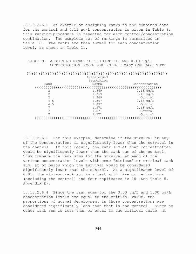
245

TABLE 9. ASSIGNING RANKS TO THE CONTROL AND 0.13 µg/LCONCENTRATION LEVEL FOR STEEL'S MANY-ONE RANK TEST

))))))))))))))))))))))))))))))))))))))))))))))))))))))))))))) Transformed Proportion Rank Normal Concentration )))))))))))))))))))))))))))))))))))))))))))))))))))))))))))))))))) 2 1.369 0.13 µg/L 2 1.369 0.13 µg/L 2 1.369 Control 4.5 1.397 0.13 µg/L 4.5 1.397 Control 7 1.571 0.13 µg/L 7 1.571 Control 7 1.571 Control ))))))))))))))))))))))))))))))))))))))))))))))))))))))))))))))))))

13.13.2.6.2 An example of assigning ranks to the combined datafor the control and 0.13 µg/L concentration is given in Table 9. This ranking procedure is repeated for each control/concentrationcombination. The complete set of rankings is summarized inTable 10. The ranks are then summed for each concentrationlevel, as shown in Table 11.

13.13.2.6.3 For this example, determine if the survival in anyof the concentrations is significantly lower than the survival inthe control. If this occurs, the rank sum at that concentrationwould be significantly lower than the rank sum of the control. Thus compare the rank sums for the survival at each of thevarious concentration levels with some "minimum" or critical ranksum, at or below which the survival would be consideredsignificantly lower than the control. At a significance level of0.05, the minimum rank sum in a test with five concentrations(excluding the control) and four replicates is 10 (See Table 5,Appendix E).

13.13.2.6.4 Since the rank sums for the 0.50 µg/L and 1.00 µg/Lconcentration levels are equal to the critical value, theproportions of normal development in those concentrations areconsidered significantly less than that in the control. Since noother rank sum is less than or equal to the critical value, no

246

TABLE 11. RANK SUMS ))))))))))))))))))))))))))))))))))))))))))))))))))))))))) Concentration µg/L Copper) Rank Sum ))))))))))))))))))))))))))))))))))))))))))))))))))))))))) 0.13 15.5 0.25 10.5 0.50 10.0 1.00 10.0

TABLE 10. TABLE OF RANKS1

))))))))))))))))))))))))))))))))))))))))))))))))))))))))))))) Copper Concentration (µg/L) ))))))))))))))))))))))))))))))))Replicate Control 0.13 0.25))))))))))))))))))))))))))))))))))))))))))))))))))))))))))))))))))))))))))

1 1.571(7,7.5,7.5,7.5,7) 1.369(2) 1.284(2) 2 1.369(2,4.5,5,5,4) 1.397(4.5) 1.345(3) 3 1.571(7,7.5,7.5,7.5,7) 1.571(7) 1.249(1) 4 1.397(4.5,6,6,6,5) 1.369(2) 1.369(4.5)

-------------------------------------------------------------------------- Copper Concentration (µg/L) (Continued) ))))))))))))))))))))))))))))))))))))))))))))))))Replicate 0.50 1.00 2.00))))))))))))))))))))))))))))))))))))))))))))))))))))))))))))))))))))))))))

1 1.266(2) 1.217(3.5) 1.571(7) 2 1.303(3.5) 1.146(2) 0.959(2) 3 1.217(1) 1.217(3.5) 1.047(3) 4 1.303(3.5) 1.133(1) 0.685(1)

))))))))))))))))))))))))))))))))))))))))))))))))))))))))))))))))))))))))))1Control ranks are given in the order of the concentration with which they were ranked.

other concentration has a significantly lower proportion normalthan the control. Because the 0.50 µg/L concentration showssignificantly lower normal development than the control while the

higher 2.00 µg/L concentration does not, these test results are

247

TABLE 12. BIVALVE MEAN LARVAL DEVELOPMENT RESPONSE AFTER SMOOTHING

Copper Conc. (µg/L) i

Response Means, Y&i (proportion)

Smoothed Means, Mi (proportion)

Control 0.13 0.25 0.50 1.00 2.00

123456

0.983 0.973 0.932 0.913 0.852 0.705

0.983 0.973 0.932 0.913 0.852 0.705

considered to have an anomalous dose-response relationship and itis recommended that the test be repeated. If an NOEC and LOECmust be determined for this test, the lowest concentration withsignificant growth impairment versus the control is considered tothe LOEC for growth. Thus, for this test, the NOEC and LOECwould be 0.25 µg/L and 0.50 µg/L, respectively.

13.13.2.7 Calculation of the ICp

13.13.2.7.1 The embryo-larval development data in Table 4 areutilized in this example. As can be seen from Table 4 and Figure2, the observed means are monotonically non-increasing withrespect to concentration (mean response for each higherconcentration is not less than or equal to the mean response for the previous concentration and the responses betweenconcentrations do not follow a linear trends). Therefore, it isnot necessary to smooth the means prior to calculating the IC. The observed means, represented by Y&i become the correspondingsmoothed means, Mi. Table 12 contains the response means andsmoothed means and Figure 3 gives a plot of the smoothed responsecurve.

13.13.2.7.2 An IC25 can be estimated using the LinearInterpolation Method. A 25% reduction in mean proportion ofnormally developed larvae, compared to the controls, would result

248

Figu

re 3

. Plo

t of r

aw d

ata,

obs

erve

d m

eans

, and

sm

ooth

ed m

eans

for t

he b

ival

ve

de

velo

pmen

t dat

a fr

om T

able

s 4

and

12.

249

in a mean proportion of 0.737, where M1(1-p/100) = 0.983(1-25/100). Examining the means and their associated concentrations(Table 12), the response, 0.737, is bracketed by C4 = 1.00 µg/Lcopper and C5 = 2.00 µg/L copper.

13.13.2.7.3 Using the equation from Section 4.2 in Appendix L,the estimate of the IC25 is calculated as follows:

ICp ' Cj%[M1(1&p/100)&Mj](C(j%1)&Cj)

(M(j%1)&Mj)

IC25 = 1.00 + [0.983(1 - 25/100) - 0.852] (2.00 - 1.00) S))))))))))))Q (0.705 - 0.852) = 1.78 µg/L.

13.13.2.7.4 When the ICPIN program was used to analyze this setof data, requesting 80 resamples, the estimate of the IC25 was1.7839 µg/L. The empirical 95.0% confidence interval for thetrue mean was not available because the number of resamples whichgenerated an IC25 estimate was not an even multiple of 40. Thecomputer program output for the IC25 for this data set is shownin Figure 4.

13.14 PRECISION AND ACCURACY

13.14.1 PRECISION

13.14.1.1 Single-Laboratory Precision

13.14.1.1.1 Single-laboratory precision data for the Mytilusspp. with the reference toxicant cadmium and lyophilized pulpmill effluent with natural seawater are provided in Tables 4-5. The coefficient of variation, based on EC25, is 32.8% to 45.0%for cadmium and 14.2% to 30.6% for lyophilized pulp milleffluent. Single-laboratory precision data for the Crassostreagigas with the reference toxicant cadmium and lyophilized pulpmill effluent with natural seawater are provided in Tables 6-7. The coefficient of variation, based on EC25, is 18.5% to 80.4%for cadmium and 20.8% to 43.3% for lyophilized pulp milleffluent.

13.14.1.2 Multi-laboratory Precision

250

Conc. ID 1 2 3 4 5 6------------------------------------------------------------------------Conc. Tested 0 0.13 0.25 0.50 1.00 2.00------------------------------------------------------------------------Response 1 1.00 0.96 0.92 0.91 0.88 1.00Response 2 0.96 0.97 0.95 0.93 0.83 0.67Response 3 1.00 1.00 0.90 0.88 0.88 0.75Response 4 0.97 0.96 0.96 0.93 0.82 0.40------------------------------------------------------------------------*** Inhibition Concentration Percentage Estimate ***Toxicant/Effluent: CopperTest Start Date: Test Ending Date: Test Species: bivalveTest Duration: 48 hoursDATA FILE: bivalve.icpOUTPUT FILE: bivalve.i25-----------------------------------------------------------------------Conc. Number Concentration Response Std. Pooled ID Replicates ug/L Means Dev. Response Means----------------------------------------------------------------------- 1 4 0.000 0.983 0.021 0.983 2 4 0.130 0.973 0.019 0.973 3 4 0.250 0.932 0.028 0.932 4 4 0.500 0.913 0.024 0.913 5 4 1.000 0.852 0.032 0.852 6 4 2.000 0.705 0.247 0.705-----------------------------------------------------------------------The Linear Interpolation Estimate: 1.7839 Entered P Value: 25-----------------------------------------------------------------------Number of Resamplings: 80Those resamples not used had estimatesabove the highest concentration/ %Effluent.

The Bootstrap Estimates Mean: 1.6188 Standard Deviation: 0.1758

No Confidence Limits can be produced since the number of resamplesgenerated is not a multiple of 40.Resampling time in Seconds: 0.17 Random_Seed: -232404862

Figure 4. ICPIN program output for the IC25.

251

13.14.1.2.1 Multi-laboratory precision data for Mytilus spp.with the reference toxicant, cadmium and lyophilized pulp milleffluent are provided in Tables 12-13. The coefficient ofvariation for cadmium EC25 is 23.6%, and for effluent EC25 is14.4% based on five laboratories. Multi-laboratory precisiondata for Crassostrea gigas with the reference toxicant, cadmiumand lyophilized pulp mill effluent are provided in Tables 14-15. The coefficient of variation is 21.3% for cadmium EC25 and 14.2%for lyophilized pulp mill effluent EC25, based on results fromfive laboratories.

13.14.2 ACCURACY

13.14.2.1 The accuracy of toxicity tests cannot be determined.

TABLE 12. SINGLE AND MULTI-LABORATORY PRECISION OF THE MUSSEL,MYTILUS SPP., DEVELOPMENT TEST PERFORMED WITH CADMIUMCHLORIDE (CD MG/L) AS A REFERENCE TOXICANT

Month Lab A Lab B Lab C Lab D Lab E

Oct-92 2.35 1.06 2.42 4.20 4.77

Nov-92 0.86 3.49 3.89 2.21 2.39

Dec-92 1.79 2.51 no data 2.27 3.73

Jan-93 3.69 2.25 6.77 no data 1.57

Feb-93 2.81 2.91 5.85 3.75 3.05

Mar-93 3.71 2.64 2.62 4.89 no data

Mean 2.54 2.48 4.31 3.46 3.10

SD 1.11 0.81 1.94 1.19 1.23

CV (%) 43.9 32.8 45.0 34.3 40.0

# of Labs Statistic EC25

5 Mean (N=5)SDCV(%)

3.180.7523.6

These data are from: Pastorok, et al. (1994), West Coast Marine SpeciesChronic Protocol Variability Study, PTI Environmental Services, Prepared forWashington Department of Ecology, February, 1994.

252

TABLE 13. SINGLE AND MULTI-LABORATORY PRECISION OF THE MUSSEL,MYTILUS SPP., DEVELOPMENT TEST PERFORMED WITHLYOPHILIZED PULP MILL EFFLUENT (%) AS THE TOXICANT

Month Lab A Lab B Lab C Lab D Lab E

Oct-92 1.78 1.40 2.02 1.83 1.85

Nov-92 1.57 1.94 2.70 1.98 no data

Dec-92 1.74 1.88 3.08 no data 1.87

Jan-93 3.17 2.03 2.46 1.07 no data

Feb-93 1.66 no data no data no data no data

Mar-93 1.85 1.66 1.72 1.82 no data

Mean 1.96 1.78 2.40 1.68 1.86

SD 0.60 0.25 0.54 0.41 0.28

CV (%) 30.6 14.2 22.5 24.5 1.4

# of Labs Statistic EC25

5 Mean (n=5)SDCV(%)

1.930.2814.4

These data are from: Pastorok, et al. (1994) West Coast MarineSpecies Chronic Protocol Variability Study, PTI EnvironmentalServices, Prepared for Washington Department of Ecology,February, 1994.

253

TABLE 14. SINGLE AND MULTI-LABORATORY PRECISION OF THE OYSTER,CRASSOSTREA GIGAS, DEVELOPMENT TEST PERFORMED WITHCADMIUM CHLORIDE (CD MG/L) AS A REFERENCE TOXICANT

Month Lab A Lab B Lab C Lab D Lab E

July-92 1.04 1.54 0.50 0.41 0.56

Aug-92 0.31 1.38 0.30 0.35 no data

Sept-92 0.68 0.20 0.49 no data no data

Apr-93 no data 0.45 0.51 no data 0.95

May-93 0.46 0.30 1.05 0.52 0.83

June-93 0.26 1.55 0.93 no data 0.83

July-93 0.28 0.82 0.66 1.56 0.90

Mean 0.51 0.89 0.63 0.71 0.81

SD 0.31 0.59 0.27 0.57 0.15

CV (%) 60.6 66.7 42.1 80.4 18.5

# of Labs Statistic EC25

5 Mean (n=5)SDCV(%)

0.710.1521.3

These data are from: Pastorok, et al. (1994), West Coast MarineSpecies Chronic Protocol Variability Study, PTI EnvironmentalServices, Prepared for Washington Department of Ecology,February, 1994.

254

TABLE 15. SINGLE AND MULTI-LABORATORY PRECISION OF THE OYSTER,CRASSOSTREA GIGAS, DEVELOPMENT TEST PERFORMED WITHLYOPHILIZED PULP MILL EFFLUENT (%) AS THE TOXICANT

Month Lab A Lab B Lab C Lab D Lab E

July-92 no data 0.91 1.28 no data 1.43

Aug-92 1.21 1.09 0.98 0.61 no data

Sept-92 0.76 1.66 0.83 no data no data

Apr-93 0.80 1.10 1.61 1.66 no data

May-93 1.21 0.65 1.90 0.93 0.93

June-93 1.09 1.32 1.72 0.83 0.98

July-93 0.82 0.80 1.56 1.67 1.04

Mean 0.98 1.08 1.41 1.14 1.10

SD. 0.21 0.34 0.40 0.49 0.23

CV (%) 21.6 31.4 28.0 43.3 20.8

# of Labs Statistic EC25

5 Mean (n=5)SDCV(%)

1.140.1614.2

These data are from: Pastorok, et al., (1994), West Coast MarineSpecies Chronic Protocol Variability Study, PTI EnvironmentalServices, Prepared for Washington Department of Ecology,February, 1994.

255

APPENDIX I. BIVALVE TEST: STEP-BY-STEP SUMMARY

PREPARATION OF TEST SOLUTIONS

A. Determine test concentrations and appropriate dilution waterbased on NPDES permit conditions and guidance from theappropriate regulatory agency.

B. Prepare effluent test solutions by diluting well mixedunfiltered effluent using volumetric flasks and pipettes. Use hypersaline brine where necessary to maintain all testsolutions at 30 ± 2‰. Include brine controls in tests thatuse brine.

C. Prepare a copper reference toxicant stock solution.

D. Prepare a series copper reference toxicant concentrations.

E. Sample effluent and reference toxicant solutions forphysical/chemical analysis. Measure salinity, pH anddissolved oxygen from each test concentration.

F. Randomize numbers for test chambers and record the chambernumbers with their respective test concentrations on arandomization data sheet. Store the data sheet safely untilafter the test samples have been analyzed.

G. Place test chambers in a water bath or environmental chamberset to 18 or 20EC and allow temperature to equilibrate.

H. Measure the temperature daily in one random replicate (orseparate chamber) of each test concentration. Monitor thetemperature of the water bath or environmental chambercontinuously.

I. At the end of the test, measure salinity, pH, and dissolvedoxygen concentration from each test concentration.

PREPARATION AND ANALYSIS OF TEST ORGANISMS

A. Determine test concentrations and appropriate dilution waterbased on NPDES permit requirements and guidance from theappropriate regulatory agency.

256

B. Prepare test solutions by diluting well mixed unfilteredeffluent using volumetric pipettes. Use hypersaline brinewhere necessary to maintain all test solutions at 30 ± 2‰. Include brine controls in tests that use brine.

C. Sample effluent and reference toxicant solutions forphysical/chemical analysis. Measure salinity, pH anddissolved oxygen from each test concentration.

D. Randomize numbers for test chambers and record the chambernumbers with their respective test concentrations on arandomization data sheet. Store the data sheet safely untilafter the test samples have been analyzed.

E. Place test chambers in a water bath or environmental chamberset to 18 or 20EC as appropriate for the test species andallow temperature to equilibrate.

F. Measure the test solution temperature daily in a randomlylocated blank test chamber. Monitor the temperature of thewater bath or environmental chamber continuously.

PREPARATION AND ANALYSIS OF TEST ORGANISMS

A. Obtain test organisms and hold or condition as necessary forspawning.

B. On day of test, spawn organisms, examine gametes, pool goodeggs, pool good sperm.

C. Fertilize subsets of eggs with a range of spermconcentrations to obtain >90% embryogenesis withoutpolyspermy.

D. Adjust embryo stock suspension density to 1500-3000/mL.

E. Introduce organisms to test chambers (150-300 embryos in 0.1mL of stock).

F. Count all embryos in each of six extra controls set up fordetermining mean embryo density and variation. Return theseto the test for later examination for developmental rate incontrols.

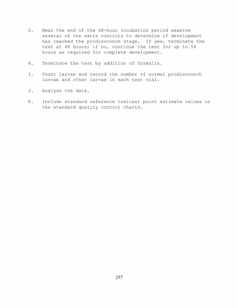
257

G. Near the end of the 48-hour incubation period examineseveral of the extra controls to determine if developmenthas reached the prodisoconch stage. If yes, terminate thetest at 48 hours; if no, continue the test for up to 54hours as required for complete development.

H. Terminate the test by addition of formalin.

I. Count larvae and record the number of normal prodisoconchlarvae and other larvae in each test vial.

J. Analyze the data.

K. Include standard reference toxicant point estimate values inthe standard quality control charts.

258

Sample data sheet for embryo microscopic examination.

BIVALVE DEVELOPMENT TEST: RESULTS

Bioassay No._______________ Date________________

Counter______________

Number Sample Abnormal Normal %Normal Notes

259

SECTION 14

RED ABALONE, Haliotis rufescensLARVAL DEVELOPMENT TEST METHOD

Adapted from a method developed byJohn W. Hunt and Brian S. Anderson

Institute of Marine Sciences, University of CaliforniaSanta Cruz, California

(in association with)California Department of Fish and GameMarine Pollution Studies Laboratory

34500 Coast Route 1, Monterey, CA 93940

TABLE OF CONTENTS

14.1 Scope and Application14.2 Summary of Method14.3 Interferences14.4 Safety14.5 Apparatus and Equipment14.6 Reagents and Supplies14.7 Effluents and Receiving Water Collection,

Preservation, and Storage14.8 Calibration and Standardization14.9 Quality Control 14.10 Test Procedures14.11 Summary of Test Conditions and Test

Acceptability Criteria14.12 Acceptability of Test Results14.13 Data Analysis14.14 Precision and Accuracy

Appendix I Step-by Step Summary

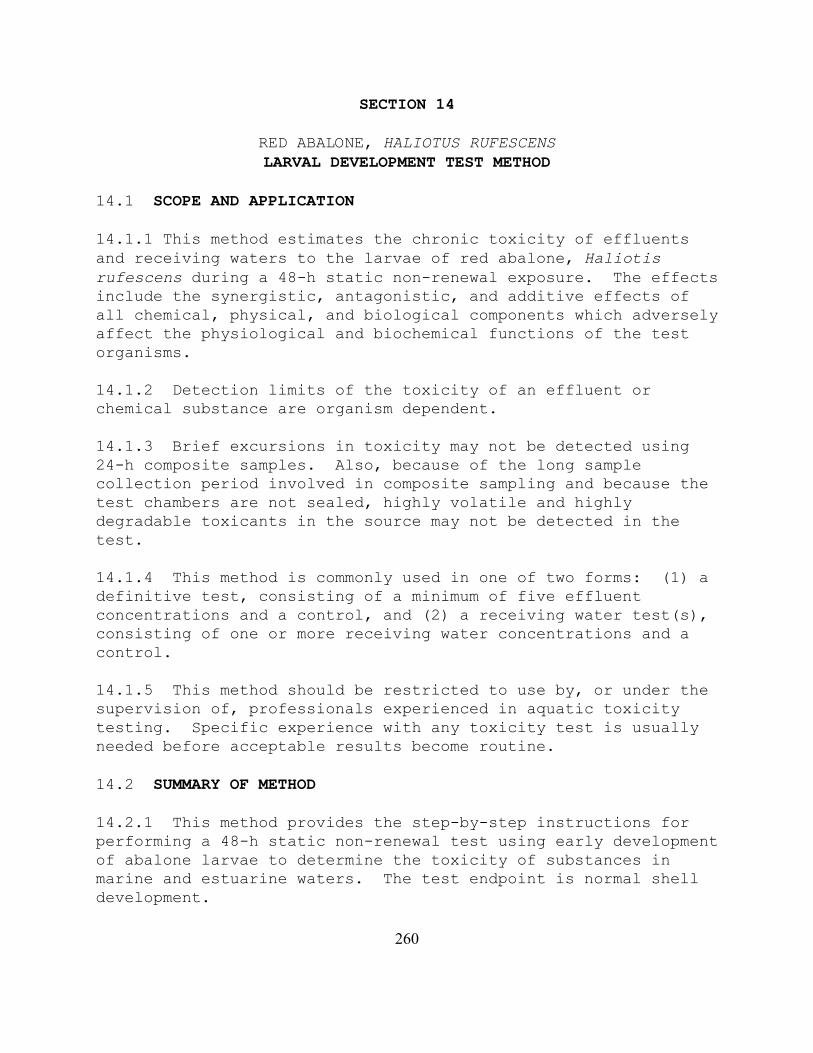
260

SECTION 14

RED ABALONE, HALIOTUS RUFESCENSLARVAL DEVELOPMENT TEST METHOD

14.1 SCOPE AND APPLICATION

14.1.1 This method estimates the chronic toxicity of effluentsand receiving waters to the larvae of red abalone, Haliotisrufescens during a 48-h static non-renewal exposure. The effectsinclude the synergistic, antagonistic, and additive effects ofall chemical, physical, and biological components which adverselyaffect the physiological and biochemical functions of the testorganisms.

14.1.2 Detection limits of the toxicity of an effluent orchemical substance are organism dependent.

14.1.3 Brief excursions in toxicity may not be detected using24-h composite samples. Also, because of the long samplecollection period involved in composite sampling and because thetest chambers are not sealed, highly volatile and highlydegradable toxicants in the source may not be detected in thetest.

14.1.4 This method is commonly used in one of two forms: (1) adefinitive test, consisting of a minimum of five effluentconcentrations and a control, and (2) a receiving water test(s),consisting of one or more receiving water concentrations and acontrol.

14.1.5 This method should be restricted to use by, or under thesupervision of, professionals experienced in aquatic toxicitytesting. Specific experience with any toxicity test is usuallyneeded before acceptable results become routine.

14.2 SUMMARY OF METHOD

14.2.1 This method provides the step-by-step instructions forperforming a 48-h static non-renewal test using early developmentof abalone larvae to determine the toxicity of substances inmarine and estuarine waters. The test endpoint is normal shelldevelopment.

261

14.3 INTERFERENCES

14.3.1 Toxic substances may be introduced by contaminants indilution water, glassware, sample hardware, and testing equipment(see Section 5, Facilities and Equipment, and Supplies).

14.3.2 Improper effluent sampling and handling may adverselyaffect test results (see Section 8, Effluent and Receiving WaterSampling, and Sample Handling, and Sample Preparation forToxicity Tests).

14.4 SAFETY

14.4.1 See Section 3, Health and Safety.

14.5 APPARATUS AND EQUIPMENT

14.5.1 Tanks, trays, or aquaria -- for holding and acclimatingadult red abalone, e.g., standard salt water aquarium or InstantOcean Aquarium (capable of maintaining seawater at 10-20EC), withappropriate filtration and aeration system.

14.5.2 Air pump, air lines, and air stones -- for aerating watercontaining broodstock or for supplying air to test solutions withlow dissolved oxygen.

14.5.3 Constant temperature chambers or water baths -- formaintaining test solution temperature and keeping dilution watersupply, gametes, and embryo stock suspensions at test temperature(15EC) prior to the test.

14.5.4 Water purification system -- Millipore Super-Q, Deionizedwater (DI) or equivalent.

14.5.5 Refractometer -- for determining salinity.

14.5.6 Hydrometer(s) -- for calibrating refractometer.

14.5.7 Thermometers, glass or electronic, laboratory grade --for measuring water temperatures.

262

14.5.8 Thermometer, National Bureau of Standards Certified (seeUSEPA METHOD l70.l, USEPA, l979) -- to calibrate laboratorythermometers.

14.5.9 pH and DO meters -- for routine physical and chemicalmeasurements.

14.5.10 Standard or micro-Winkler apparatus -- for determiningDO (optional) and calibrating the DO meter.

14.5.11 Winkler bottles -- for dissolved oxygen determinations.

14.5.12 Balance -- Analytical, capable of accurately weighing to0.0001 g.

14.5.13 Fume hood -- to protect the analyst from effluent orformaldehyde fumes.

14.5.14 Glass stirring rods -- for mixing test solutions.

14.5.15 Graduated cylinders -- Class A, borosilicate glass ornon-toxic plastic labware, 50-l000 mL for making test solutions. (Note: not to be used interchangeably for gametes or embryos andtest solutions).

14.5.16 Volumetric flasks -- Class A, borosilicate glass or non-toxic plastic labware, 10-1000 mL for making test solutions.

14.5.17 Pipets, automatic -- adjustable, to cover a range ofdelivery volumes from 0.010 to 1.000 mL.

14.5.18 Pipet bulbs and fillers -- PROPIPET® or equivalent.

14.5.19 Wash bottles -- for reagent water, for topping offgraduated cylinders, for rinsing small glassware and instrumentelectrodes and probes.

14.5.20 Wash bottles -- for dilution water.

14.5.21 20-liter cubitainers or polycarbonate water cooler jugs-- for making hypersaline brine.

263

14.5.22 Cubitainers, beakers, or similar chambers of non-toxiccomposition for holding, mixing, and dispensing dilution waterand other general non-effluent, non-toxicant contact uses. Theseshould be clearly labeled and not used for other purposes.

14.5.23 Beakers, 1,000 mL borosilicate glass -- for mixinggametes for fertilization of eggs.

14.5.24 Beakers, 250 mL borosilicate glass -- for preparation oftest solutions.

14.5.25 Counter, two unit, 0-999 -- for recording counts oflarvae.

14.5.26 Inverted or compound microscope -- for inspectinggametes and making counts of larvae.

14.5.27 Perforated plunger -- for stirring egg solutions.

14.5.28 Supply of Macrocystis or other macroalgae (if holdingbroodstock for longer than 5 days) -- for feeding abalone.

14.5.29 Stainless steel butter knife, rounded smooth-edged blade(for handling adult abalone). Abalone irons and plastic puttyknives have also been used successfully.

14.5.30 Sieve or screened tube, approximately 37 µm-mesh -- forretaining larvae at the end of the test.

14.5.31 60 µm NITEX® filter -- for filtering receiving water.

14.6 REAGENTS AND SUPPLIES

14.6.1 Sample containers -- for sample shipment and storage (seeSection 8, Effluent and Receiving Water Sampling, and SampleHandling, and Sample Preparation for Toxicity Tests).

14.6.2 Data sheets (one set per test) -- for data recording (SeeAppendix I).

14.6.3 Tape, colored -- for labelling test chambers andcontainers.

264

14.6.4 Markers, water-proof -- for marking containers, etc.

14.6.5 Parafilm -- to cover graduated cylinders and vesselscontaining gametes, embryos.

14.6.6 Gloves, disposable -- for personal protection fromcontamination.

14.6.7 Pipets, serological -- l-l0 mL, graduated.

14.6.8 Pipet tips -- for automatic pipets.

14.6.9 Coverslips -- for microscope slides.

14.6.10 Lens paper -- for cleaning microscope optics.

14.6.11 Laboratory tissue wipes -- for cleaning and dryingelectrodes, microscope slides, etc.

14.6.12 Disposable countertop covering -- for protection of worksurfaces and minimizing spills and contamination.

14.6.13 pH buffers 4, 7, and l0 (or as per instructions ofinstrument manufacturer) -- for standards and calibration check(see USEPA Method l50.l, USEPA, l979).

14.6.14 Membranes and filling solutions -- for dissolved oxygenprobe (see USEPA Method 360.l, USEPA, l979), or reagents formodified Winkler analysis.

14.6.15 Laboratory quality assurance samples and standards --for the above methods.

14.6.16 Test chambers -- 600 mL, five chambers perconcentration. The chambers should be borosilicate glass (foreffluents) or nontoxic disposable plastic labware (for referencetoxicants). To avoid contamination from the air and excessiveevaporation of test solutions during the test, the chambersshould be covered during the test with safety glass plates or aplastic sheet (6 mm thick).

14.6.17 Formaldehyde, 37% (Concentrated Formalin) -- forpreserving larvae. Note: formaldehyde has been identified as a

265

carcinogen and is irritating to skin and mucous membranes. Itshould not be used at a concentration higher than necessary toachieve morphological preservation of larvae for counting andonly under conditions of maximal ventilation and minimalopportunity for volatilization into room air.

14.6.18 Tris (hydroxymethyl) aminomethane and hydrogen peroxide(for H2O2 spawning method) -- for spawning abalone.

14.6.19 Reference toxicant solutions (see Subsection 14.10.2.4and see Section 4, Quality Assurance).

14.6.20 Reagent water -- defined as distilled or deionized waterthat does not contain substances which are toxic to the testorganisms (see Section 5, Facilities, Equipment, and Supplies andSection 7, Dilution Water).

14.6.21 Effluent and receiving water -- see Section 8, Effluentand Surface Water Sampling, and Sample Handling, and SamplePreparation for Toxicity Tests.

14.6.22 Dilution water and hypersaline brine -- see Section 7,Dilution Water and Section 14.6.24, Hypersaline Brines. The dilution water should be uncontaminated 1-µm-filtered naturalseawater. Hypersaline brine should be prepared from dilutionwater.

14.6.23 HYPERSALINE BRINES

14.6.23.1 Most industrial and sewage treatment effluentsentering marine and estuarine systems have little measurablesalinity. Exposure of larvae to these effluents will usuallyrequire increasing the salinity of the test solutions. It isimportant to maintain an essentially constant salinity across alltreatments. In some applications it may be desirable to matchthe test salinity with that of the receiving water (See Section7.1). Two salt sources are available to adjust salinities --artificial sea salts and hypersaline brine (HSB) derived fromnatural seawater. Use of artificial sea salts is necessary onlywhen high effluent concentrations preclude salinity adjustment byHSB alone.

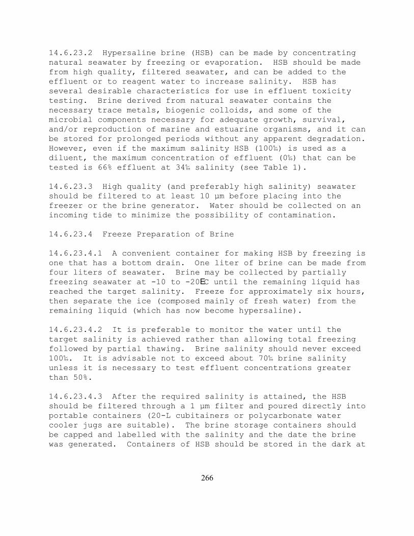
266

14.6.23.2 Hypersaline brine (HSB) can be made by concentratingnatural seawater by freezing or evaporation. HSB should be madefrom high quality, filtered seawater, and can be added to theeffluent or to reagent water to increase salinity. HSB hasseveral desirable characteristics for use in effluent toxicitytesting. Brine derived from natural seawater contains thenecessary trace metals, biogenic colloids, and some of themicrobial components necessary for adequate growth, survival,and/or reproduction of marine and estuarine organisms, and it canbe stored for prolonged periods without any apparent degradation. However, even if the maximum salinity HSB (100‰) is used as adiluent, the maximum concentration of effluent (0‰) that can betested is 66% effluent at 34‰ salinity (see Table 1).

14.6.23.3 High quality (and preferably high salinity) seawatershould be filtered to at least 10 µm before placing into thefreezer or the brine generator. Water should be collected on anincoming tide to minimize the possibility of contamination.

14.6.23.4 Freeze Preparation of Brine

14.6.23.4.1 A convenient container for making HSB by freezing isone that has a bottom drain. One liter of brine can be made fromfour liters of seawater. Brine may be collected by partiallyfreezing seawater at -10 to -20EC until the remaining liquid hasreached the target salinity. Freeze for approximately six hours,then separate the ice (composed mainly of fresh water) from theremaining liquid (which has now become hypersaline).

14.6.23.4.2 It is preferable to monitor the water until thetarget salinity is achieved rather than allowing total freezingfollowed by partial thawing. Brine salinity should never exceed100‰. It is advisable not to exceed about 70‰ brine salinityunless it is necessary to test effluent concentrations greaterthan 50%.

14.6.23.4.3 After the required salinity is attained, the HSBshould be filtered through a 1 µm filter and poured directly intoportable containers (20-L cubitainers or polycarbonate watercooler jugs are suitable). The brine storage containers shouldbe capped and labelled with the salinity and the date the brinewas generated. Containers of HSB should be stored in the dark at

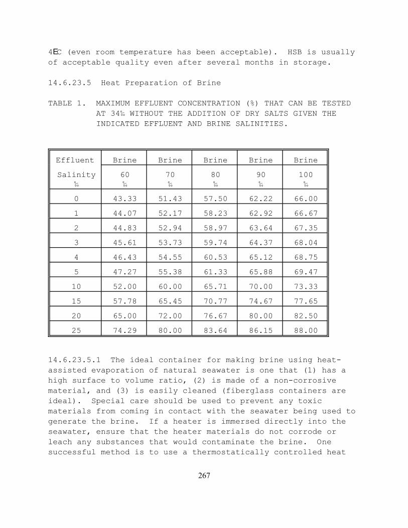
267

4EC (even room temperature has been acceptable). HSB is usuallyof acceptable quality even after several months in storage.

14.6.23.5 Heat Preparation of Brine

TABLE 1. MAXIMUM EFFLUENT CONCENTRATION (%) THAT CAN BE TESTED AT 34‰ WITHOUT THE ADDITION OF DRY SALTS GIVEN THE INDICATED EFFLUENT AND BRINE SALINITIES.

Effluent Brine Brine Brine Brine Brine

Salinity‰

60‰

70‰

80‰

90‰

100‰

0 43.33 51.43 57.50 62.22 66.00

1 44.07 52.17 58.23 62.92 66.67

2 44.83 52.94 58.97 63.64 67.35

3 45.61 53.73 59.74 64.37 68.04

4 46.43 54.55 60.53 65.12 68.75

5 47.27 55.38 61.33 65.88 69.47

10 52.00 60.00 65.71 70.00 73.33

15 57.78 65.45 70.77 74.67 77.65

20 65.00 72.00 76.67 80.00 82.50

25 74.29 80.00 83.64 86.15 88.00

14.6.23.5.1 The ideal container for making brine using heat-assisted evaporation of natural seawater is one that (1) has ahigh surface to volume ratio, (2) is made of a non-corrosivematerial, and (3) is easily cleaned (fiberglass containers areideal). Special care should be used to prevent any toxicmaterials from coming in contact with the seawater being used togenerate the brine. If a heater is immersed directly into theseawater, ensure that the heater materials do not corrode or leach any substances that would contaminate the brine. Onesuccessful method is to use a thermostatically controlled heat

268

exchanger made from fiberglass. If aeration is needed, use onlyoil-free air compressors to prevent contamination. 14.6.23.5.2 Before adding seawater to the brine generator,thoroughly clean the generator, aeration supply tube, heater, andany other materials that will be in direct contact with thebrine. A good quality biodegradable detergent should be used,followed by several (at least three) thorough reagent waterrinses.

14.6.23.5.3 Seawater should be filtered to at least 10 µm beforebeing put into the brine generator. The temperature of theseawater is increased slowly to 40EC. The water should beaerated to prevent temperature stratification and to increasewater evaporation. The brine should be checked daily (dependingon the volume being generated) to ensure that the salinity doesnot exceed 100‰ and that the temperature does not exceed 40EC. Additional seawater may be added to the brine to obtain thevolume of brine required.

14.6.23.5.4 After the required salinity is attained, the HSBshould be filtered through a 1 µm filter and poured directly intoportable containers (20-L cubitainers or polycarbonate watercooler jugs are suitable). The brine storage containers shouldbe capped and labelled with the salinity and the date the brinewas generated. Containers of HSB should be stored in the dark at4EC (even room temperature has been acceptable). HSB is usuallyof acceptable quality even after several months in storage.

14.6.23.6 Artificial Sea Salts

14.6.23.6.1 No data from red abalone tests using sea salts orartificial seawater (e.g., GP2) are available for evaluation atthis time, and their use must be considered provisional.

14.6.23.7 Dilution Water Preparation from Brine

14.6.23.7.1 Although salinity adjustment with brine is thepreferred method, the use of high salinity brines and/or reagentwater has sometimes been associated with discernible adverseeffects on test organisms. For this reason, it is recommendedthat only the minimum necessary volume of brine and reagent waterbe used to offset the low salinity of the effluent, and that

269

brine controls be included in the test. The remaining dilutionwater should be natural seawater. Salinity may be adjusted inone of two ways. First, the salinity of the highest effluenttest concentration may be adjusted to an acceptable salinity, andthen serially diluted. Alternatively, each effluentconcentration can be prepared individually with appropriatevolumes of effluent and brine.

14.6.23.7.2 When HSB and reagent water are used, thoroughlymix together the reagent water and HSB before mixing in theeffluent. Divide the salinity of the HSB by the expected testsalinity to determine the proportion of reagent water to brine. For example, if the salinity of the brine is 100‰ and the test isto be conducted at 34‰, 100‰ divided by 34‰ = 2.94. Theproportion of brine is 1 part plus 1.94 parts reagent water. Tomake 1 L of dilution water at 34‰ salinity from a HSB of 100‰,340 mL of brine and 660 mL of reagent water are required. Verifythe salinity of the resulting mixture using a refractometer.

14.6.23.8 Test Solution Salinity Adjustment

14.6.23.8.1 Table 2 illustrates the preparation of testsolutions (up to 50% effluent) at 34‰ by combining effluent, HSB,and dilution water. Note: if the highest effluent concentrationdoes not exceed 50% effluent, it is convenient to prepare brineso that the sum of the effluent salinity and brine salinityequals 68‰; the required brine volume is then always equal to theeffluent volume needed for each effluent concentration as in theexample in Table 2.

14.6.23.8.2 Check the pH of all test solutions and adjust towithin 0.2 units of dilution water pH by adding, dropwise, dilutehydrochloric acid or sodium hydroxide (see Section 8.8.9,Effluent and Receiving Water Sampling, Sample Handling, andSample Preparation for Toxicity Tests).

14.6.23.8.3 To calculate the amount of brine to add to eacheffluent dilution, determine the following quantities: salinityof the brine (SB, in ‰), the salinity of the effluent (SE, in ‰), and volume of the effluent to be added (VE, in mL). Then use the following formula to calculate the volume of brine (VB,in mL) to be added:

270

VB = VE x (34 - SE)/(SB - 34)

14.6.23.8.4 This calculation assumes that dilution watersalinity is 34 ± 2‰.

14.6.23.9 Preparing Test Solutions

14.6.23.9.1 Two hundred mL of test solution are needed for eachtest chamber. To prepare test solutions at low effluentconcentrations (<6%), effluents may be added directly to dilutionwater. For example, to prepare 1% effluent, add 10 mL ofeffluent to a 1-liter volumetric flask using a volumetric pipetor calibrated automatic pipet. Fill the volumetric flask to the1-L mark with dilution water, stopper it, and shake to mix. Distribute equal volumes into the replicate test chambers.

14.6.23.9.2 To prepare a test solution at higher effluentconcentrations, hypersaline brine must usually be used. Forexample, to prepare 40% effluent, add 400 mL of effluent to a 1-liter volumetric flask. Then, assuming an effluent salinity of2‰ and a brine salinity of 66‰, add 400 mL of brine (see equationabove and Table 2) and top off the flask with dilution water. Stopper the flask and shake well. Distribute equal volumes intothe replicate test chambers.

14.6.23.10 Brine Controls

14.6.23.10.1 Use brine controls in all tests where brine isused. Brine controls contain the same volume of brine as doesthe highest effluent concentration using brine, plus the volumeof reagent water needed to reproduce the hyposalinity of theeffluent in the highest concentration, plus dilution water. Calculate the amount of reagent water to add to brine controls byrearranging the above equation, (See, 16.6.23.8.3) setting SE =0, and solving for VE.

VE = VB x (SB - 34)/(34 - SE)

If effluent salinity is essentially 0‰, the reagent water volumeneeded in the brine control will equal the effluent volume at thehighest test concentration. However, as effluent salinity andeffluent concentration increase, less reagent water volume isneeded.

271

14.6.24 TEST ORGANISMS

14.6.24.1 The test organisms used for this test are red abalone,Haliotis rufescens. This large gastropod mollusc is harvestedcommercially in southern California and supports a popularrecreational fishery throughout the state. It consumes a varietyof seaweeds and small incidental organisms, and is an importantfood source for sea otters, lobsters, and octopods (Hines andPearse 1892). Abalone are "broadcast" spawners that reproduce by equivalent.ejecting large numbers of gametes into the watercolumn, where fertilization takes place externally. Free-swimming larvae hatch as trochophores, then undergo torsion whilepassing through a veliger stage. Abalone larvae do not feedduring their one to three weeks in the plankton, but exist onenergy stored in the yolk sack, supplemented perhaps by theuptake of dissolved amino acids. Once larvae come into contactwith suitable substrate, they metamorphose and begin to consumebenthic algae using a rasp-like tongue (the radula). Red abalonebecome reproductive after about two years at a length of about 7cm, and can live for at least 25 years, growing to 30 cm inlength. Refer to Hahn (1989) for a review of abalone life historyand culture to Martin et al. (1977), Morse et al (1979) and Huntand Anderson (1989 and 1993) for previous toxicity studies.

14.6.24.2 Species Identification

14.6.24.2.1 Broodstock should be positively identified tospecies. Epipodal characteristics provide the best means ofidentification. All California haliotids have a lacey epipodialfringe, except for the red and black abalone, which have smooth,lobed epipodia. The red abalone can be distinguished from theblack by shell coloration and by the number of respiratory pores in the shell (reds have 3 to 4, blacks have 5 to 8). For furtherinformation on abalone taxonomy consult Owen et al. (1971), andMorris et al. (1980).

14.6.24.3 Obtaining Broodstock

14.6.24.3.1 Mature red abalone broodstock can be collected fromrocky substrates from the intertidal to depths exceeding 30meters. They are found most commonly in crevices in areas wherethere is an abundance of macroalgae. State collection permitsare usually required for collecting abalone. Collection of

272

TABLE 2. EXAMPLES OF EFFLUENT DILUTION SHOWING VOLUMES OFEFFLUENT (x‰), BRINE, AND DILUTION WATER NEEDED FOR ONELITER OF EACH TEST SOLUTION.

FIRST STEP: Combine brine with reagent water or natural seawater to achieve abrine of 68-x‰ and, unless natural seawater is used for dilution water, also abrine-based dilution water of 34‰.

SERIAL DILUTION:

Step 1. Prepare the highest effluent concentration to be tested by addingequal volumes of effluent and brine to the appropriate volume of dilutionwater. An example using 40% is shown.

Effluent Conc.(%)

Effluent x‰ Brine (68-x)‰

Dilution Water*34‰

40 800 mL 800 mL 400 mL

Step 2. Use either serially prepared dilutions of the highest testconcentration or individual dilutions of 100% effluent.

Effluent Conc. (%) Effluent Source Dilution Water* (34‰)

20 1000 mL of 40% 1000 mL

10 1000 mL of 20% 1000 mL

5 1000 mL of 10% 1000 mL

2.5 1000 mL of 5% 1000 mL

Control none 1000 mLINDIVIDUAL PREPARATION

Effluent Conc.(%)

Effluent x‰ Brine (68-x)‰ Dilution Water*34‰

40 400 mL 400 mL 200 mL

20 200 mL 200 mL 600 mL

10 100 mL 100 mL 800 mL

5 50 mL 50 mL 900 mL

2.5 25 mL 25 mL 950 mL

Control none none 1000 mL*May be natural seawater or brine-reagent water.

273

abalone is regulated by California law. Collectors must obtain ascientific collectors permit from the California Department ofFish and Game and observe any regulations regarding collection,transfer, and maintenance of abalone broodstock.

14.6.24.3.2 While abalone captured in the wild can be induced tospawn, those grown or conditioned in the laboratory have beenmore dependable. Commercial mariculture facilities in Californiaproduce large numbers of abalone, and distribution systems existto supply live spawners to a number of market areas. In anycase, broodstock should be obtained from sources free ofcontamination by toxic substances to avoid genetic orphysiological preadaptation to pollutants.

14.6.24.3.3 Abalone broodstock can be transported for short timeperiods from the field or supply facility in clean coveredplastic buckets filled with seawater. Use compressed air, orbattery powered pumps to supply aeration. Compressed oxygen isnot recommended because bubbled oxygen may induce unintendedspawning (Morse et al., 1977). Maintain water temperatureswithin 3EC of the temperature at the collecting site. Fourabalone in a 15-liter bucket should remain healthy for up to fourhours under these conditions.

14.6.24.3.4 Abalone can be transported for up to 30 hours insealed, oxygen-filled plastic bags containing moist (seawater)polyfoam sponges (Hahn, 1989). Cut the polyfoam into sections(about 20 X 40 cm) and allow them to soak in clean seawater for afew minutes. New sponges should be leached in seawater for atleast 24 hours. Rinse the sponges in fresh seawater and wringthem out well. Place the polyfoam inside double plastic trashbags, then place the abalone on the moist foam. It is importantthat there is no standing water in the bags. Put the abalonebags into an ice chest (10 to 15 liter), fill the bags with pureoxygen, squeeze the bags to purge out all the air, then refillwith oxygen (approximately three liters of oxygen gas willsupport eight abalone). Seal the bags (air-tight) with a tie orrubber band. Wrap two small (one-liter) blue ice blocks insections of newspaper (about 15 pages thick) for insulation, andplace the wrapped blue ice in a sealed plastic bag in the chest on top of the abalone bags. Fill any remaining space withpacking and seal the box for shipping. Avoid transporting theice chest in temperatures below freezing or above 30EC.

274

14.6.24.4 Broodstock Culture and Handling

14.6.24.4.1 At the testing facility, place the abalone inaerated tanks with flowing seawater (1 to 2 liter/min). Withhigh water quality, water flow, and aeration, abalone 8 to 10 cmlong can be kept at a density of one per liter of tank space orone per 100 cm2 of tank surface area, whichever provides thelower density. Density should be cut to a maximum of 0.5 perliter in recirculating systems and to a maximum of 0.25 per literin static tanks. Tanks should be covered for shade and toprevent escape. Drain and rinse culture tanks twice weekly toprevent build-up of detritus. Remove any dead abaloneimmediately, and drain and scrub its tank.

14.6.24.4.2 Ideal maintenance temperature is 15 ± 1EC, thetoxicity test temperature (see also Leighton, 1974). Ifbroodstock are to be held for longer than 5 days at the testingfacility, feed broodstock with blades of the giant kelp,Macrocystis. Feed to slight excess; large amounts of uneatenalgae will foul culture water. If Macrocystis is unavailable,other brown algae (Nereocystis, Egregia, Eisenia) or any fleshyred algae can be substituted (Hahn, 1989).

14.6.24.4.3 Recirculating tanks should be equipped withbiological or activated carbon filtration systems and oystershell beds to maintain water quality. Measure the ammoniacontent of static or recirculating seawater daily to monitor theeffectiveness of the filtration system. Un-ionized ammoniaconcentrations should not exceed 20 µg/liter and total ammoniaconcentrations should not exceed 1.0 mg/liter. Supply constantaeration and temperature control. Add only a few blades of algalfood at each cleaning to prevent its accumulation and decay.

14.6.24.4.4 When handling abalone, use a rounded, dull-bladedstainless-steel butter knife, abalone iron, or plastic puttyknife to release the animal's grip on the substrate. Gentlyslide the flat dull blade under the foot at the posterior endnear the beginning of the shell whorl, and slide it under abouttwo-thirds of the foot. Apply constant pressure to keep thefront edge of the blade against the substrate and not up into thefoot. Quickly and gently lift the foot off the substrate. Asmooth deliberate motion is more effective and less damaging thanrepeated prying.

275

14.6.24.4.5 Assess the reproductive condition of the broodstockby examining the gonads, located under the right posterior edgeof the shell. An abalone placed upside down on a flat surfacewill soon relax and begin moving the foot trying to right itself. Take advantage of this movement and use the dull blade to bendthe foot away from the gonad area for inspection. The femaleovary is jade green, the male testes are cream-colored. When thegonad fully envelopes the dark blue-gray conical digestive glandand is bulky along its entire length, the abalone is ready forspawning (Hahn, 1989). Ripe (recrudescent) spawners have adistinct color difference between the gray digestive gland andthe green or cream-colored gonad. Less developed gonads appeargray (in females) or brown (in males).

14.6.24.4.6 Abalone 7 to 10 cm in shell length are recommendedin broodstock. They are easier to handle than larger ones, andcan be spawned more often (approximately every four months undersuitable culture conditions; Ault, 1985). Though spawning fewereggs than larger abalone, 10 cm abalone will produce over 100,000eggs at a time (Ault, 1985). Twenty to thirty-five thousand eggs are needed for a single toxicant test, depending on test design. For further information of red abalone culture, see Ebert andHouk (1984) or Hahn (1989).

14.6.24.5 Culture Materials

14.6.24.5.1 See Section 4, Quality Assurance Section for adiscussion of suitable materials to be used in laboratory cultureof abalone. Be sure all new materials are properly leached inseawater before use. After use, all culture materials should bewashed in soap and water, then rinsed with seawater before reuse.

14.7 EFFLUENT AND RECEIVING WATER COLLECTION, PRESERVATION, AND STORAGE

14.7.1 See Section 8, Effluent and Receiving Water Sampling,Sample Handling, and Sample Preparation for Toxicity Tests.

14.8 CALIBRATION AND STANDARDIZATION

14.8.1 See Section 4, Quality Assurance.

14.9 QUALITY CONTROL

276

14.9.1 See Section 4, Quality Assurance.

14.10 TEST PROCEDURES

14.10.1 TEST DESIGN

14.10.1.1 The test consists of at least five effluentconcentrations plus a dilution water control. Tests that usebrine to adjust salinity must also contain five replicates of abrine control.

14.10.1.2 Effluent concentrations are expressed as percenteffluent.

14.10.2 TEST SOLUTIONS

14.10.2.1 Receiving waters

14.10.2.1.1 The sampling point is determined by the objectivesof the test. At estuarine and marine sites, samples are usuallycollected at mid-depth. Receiving water toxicity is determinedwith samples used directly as collected or with samples passedthrough a 60 µm NITEX® filter and compared without dilution, against a control. Using five replicate chambers per test, eachcontaining 200 mL would require approximately 1 L of sample pertest.

14.10.2.2 Effluents

14.10.2.2.1 The selection of the effluent test concentrationsshould be based on the objectives of the study. A dilutionfactor of at least 0.5 is commonly used. A dilution factor of0.5 provides hypothesis test discrimination of ± 100%, andtesting of a 16 fold range of concentrations. Hypothesis testdiscrimination shows little improvement as dilution factors areincreased beyond 0.5 and declines rapidly if smaller dilutionfactors are used. USEPA recommends that one of the five effluenttreatments must be a concentration of effluent mixed withdilution water which corresponds to the permittee's instreamwaste concentration (IWC). At least two of the effluenttreatments must be of lesser effluent concentration than the IWC,

277

with one being at least one-half the concentration of the IWC. If 100‰ HSB is used as a diluent, the maximum concentration ofeffluent that can be tested will be 66% at 34‰ salinity.

14.10.2.2.2 If the effluent is known or suspected to be highlytoxic, a lower range of effluent concentrations should be used(such as 25%, 12.5%, 6.25%, 3.12% and 1.56%).

14.10.2.2.3 The volume in each test chamber is 200 mL.

14.10.2.2.4 Effluent dilutions should be prepared for allreplicates in each treatment in one container to minimizevariability among the replicates. Dispense into the appropriateeffluent test chambers.

14.10.2.3 Dilution Water

14.10.2.3.1 Dilution water should be uncontaminated 1-µm-filtered natural seawater or hypersaline brine prepared fromuncontaminated natural seawater plus reagent water (see Section7, Dilution Water). Natural seawater may be uncontaminatedreceiving water. This water is used in all dilution steps and asthe control water.

14.10.2.4 Reference Toxicant Test

14.10.2.4.1 Reference toxicant tests should be conducted asdescribed in Quality Assurance (see Section 4.7).

14.10.2.4.2 The preferred reference toxicant for red abalone iszinc sulfate (ZnSO4NH2O). Reference toxicant tests provide anindication of the sensitivity of the test organisms and thesuitability of the testing laboratory (see Section 4 QualityAssurance). Another toxicant may be specified by theappropriate regulatory agency. Prepare a 10,000 µg/L zinc stocksolution by adding 0.0440 g of zinc sulfate (ZnSO4NH2O) to oneliter of reagent water in a polyethylene volumetric flask. Alternatively, certified standard solutions can be ordered fromcommercial companies.

14.10.2.4.3 Reference toxicant solutions should be fivereplicates each of 0 (control), 10, 18, 32, and 56, and 100 µg/Ltotal zinc. Prepare one liter of each concentration by adding 0,

278

1.0, 1.8, 3.2, 5.6, and 10.0 mL of stock solution, respectively,to one-liter volumetric flasks and fill with dilution water. Start with control solutions and progress to the highestconcentration to minimize contamination.

14.10.2.4.4 If the effluent and reference toxicant tests are tobe run concurrently, then the tests must use embryos from thesame spawn. The tests must be handled in the same way and testsolutions delivered to the test chambers at the same time. Reference toxicant tests must be conducted at 34 ± 2‰.

14.10.3 COLLECTION OF GAMETES FOR THE TEST

14.10.3.1 Spawning Induction

14.10.3.1.1 Note: Before beginning the spawning inductionprocess, be sure that test solutions will be mixed, sampled, andtemperature equilibrated in time to receive the newly fertilizedeggs. Spawning induction generally takes about three hours, butif embryos are ready before test solutions are at the propertemperature, the delay may allow embryos to develop past the one-cell stage before transfer to the toxicant. Transfer can thendamage the embryos, leading to unacceptable test results.

14.10.3.1.2 Culture work (spawning, etc.) and toxicant workshould be done in separate laboratory rooms, and care should betaken to avoid contaminating organisms prior to testing.

14.10.3.1.3 Ripe abalone can be induced to spawn by stimulatingthe synthesis of prostoglandin-endoperoxide in the reproductivetissues (Morse et al., 1977). This can be done in two ways: addition of hydrogen peroxide to seawater buffered with Tris(Morse et al., 1977), or irradiation of seawater with ultravioletlight (Kikuchi and Uki, 1974). The first method is preferablefor small laboratories because it avoids the cost and maintenancerequirements of a UV system. If a UV system is available, thismethod may be preferable because it is simple, does not usechemicals that could accidentally harm larvae, and is consideredto be less likely to force gametes from unripe adults.

14.10.3.1.4 If brood stock are shipped to the laboratory by asupplier, it is important to allow two days or more forlaboratory acclimation before spawning induction; this should

279

increase the probability of achieving a successful spawn ofviable gametes. Always bring brood stock up to acclimationtemperature slowly to avoid premature spawning.

14.10.3.2 Hydrogen Peroxide Method

14.10.3.2.1 Select four ripe male abalone and four ripe females. Clean their shells of any loose debris. Place the males in oneclean polyethylene bucket and the females in another. Cover thebuckets with a tight fitting perforated lid, supply the chamberswith flowing or recirculating (1 liter/minute) 20-µm-filteredseawater (15EC), and leave the animals without food for 24 to 48hours to acclimate and eliminate wastes. If flowing seawater isunavailable, keep the spawners in larger (>30 liter) aquaria withaeration at 15 ± 1EC for 24 hours without food to eliminatewastes. Three hours prior to the desired spawning time, drainthe buckets, wipe and rinse out mucus and debris, and refill with6 liters of 1 µm-filtered seawater. If abalone have been kept inlarger aquaria, put them in the buckets at this time. Check theabalone from time to time to make sure they remain underwater. Add air stones to the buckets and keep them aerated untilspawning begins.

14.10.3.2.1 Dissolve 12.1 g of Tris into 50 mL of reagent water. When the Tris has dissolved completely, mix the hydrogen peroxide(H2O2) solution in a separate flask by pouring 10 mL of fresh*refrigerated H2O2 (30%) into 40 mL of refrigerated reagent water(1:5 dilution). Pour 25 mL of Tris solution and 25 mL of H2O2

solution into each of the spawning buckets (male and female). Stir well to mix; the final concentration in the spawning bucketswill be approximately 6 mM Tris (pH = 9.1) and 5 m H2O2. Allowthe abalone to remain in contact with the chemicals for 2.5 hoursat 15 ± 1EC. The chemical reaction is temperature dependent(three hours of contact with H2O2 would be necessary at 11EC). Temperatures higher than 15EC are not recommended for spawning. Maintain constant aeration. Since females often begin spawningafter the males, it may be useful to induce male spawning 15-30minutes later, however egg quality should not be compromised iffemales spawn first (See 14.10.3.3.2 below).

*Note: Hydrogen peroxide loses potency over time. Purchasereagent or certified grade H2O2 in small containers (100

280

mL). Store unopened containers for no more than one year,and discard open containers after one month. Mark thepurchase date and opening date on all containers, and keepall containers refrigerated.

14.10.3.2.3 After 2.5 hours, empty the spawning buckets, rinsethem well, and refill them to the top with fresh dilution waterseawater at the same temperature (15 ± 1EC). Keep the containersclean by siphoning away mucus and debris. Maintain constantaeration until spawning begins, then remove the air stones. Theabalone begin spawning about three hours after the introductionof the chemicals (at 15 ± 1EC). Eggs are dark green and arevisible individually to the naked eye, sperm appear as whiteclouds emanating from the respiratory pores.

14.10.3.2.4 If spawning begins before the chemicals have beenremoved, drain the buckets immediately, discarding any gametes. Rinse the buckets thoroughly and refill with clean, dilutionwater seawater (15 ± 1EC). Use only the gametes subsequentlyspawned in clean water for testing.

14.10.3.3 UV Irradiation Method

14.10.3.3.1 Select four ripe male abalone and four ripe females. Clean their shells of any debris. Place the males in one cleanpolyethylene bucket and the females in another. Cover thebuckets with a tight fitting perforated lid, supply thecontainers with flowing or recirculating (1 liter/minute) 20-µm-filtered seawater (15 ± 1EC), and leave the animals without foodfor 24 to 48 hours to acclimate and eliminate wastes. If flowingseawater is unavailable, keep the spawners in larger (>30 liter)aquaria with aeration at 15 ± 1EC for 24 hours. Three hoursprior to the desired spawning time, drain the buckets, wipe andrinse out mucus and debris, and refill with just enough water tocover the abalone (which should all be placed in the bottom ofthe bucket). Begin slowly filling the buckets with dilutionwater seawater (15 ± 1EC) that has passed through the UVsterilization unit. Flow rates to each of the buckets should be150 mL/min. A low total flow rate (300 mL/minute) in the UV unitis necessary to permit sufficient seawater irradiation. (Thesterilization unit should be cleaned and the UV bulb replaced atleast once annually). Place the buckets in a water bath at 15 ±1EC to counter the temperature increase caused by the slow

281

passage of the water past the UV lamp. Check the containersperiodically, and keep them clean by siphoning out any debris. After three hours (± about 1/2 hour), abalone should beginspawning by ejecting clouds of gametes into the water. Eggs aredark green and are visible individually to the naked eye, spermappear as white clouds emanating from the respiratory pores.

14.10.3.3.2 Note: If past experience or other factors indicatedifficulties in achieving synchronous spawning, it may be helpfulto induce a second group of females about an hour after thefirst. This will increase the chances of providing fresh eggs(less than one hour old) for fertilization if males spawn late(see below). Senescence of sperm is seldom a problem becausemales continue spawning over a longer period of time.

14.10.3.4 Pooling Gametes

14.10.3.4.1 Although it is not necessary, it is preferable tohave more than one abalone of each sex spawn. To increase theprobability of multiple spawners without risking senescence ofthe gametes, allow one-half hour after the first individual ofthe second sex begins to spawn before initiating fertilization. For example, if males spawn first, wait one-half hour after thefirst female spawns before fertilizing eggs. In most cases thiswill provide time for more than one of each sex to spawn. Moreimportant than multiple spawning, however, is avoiding delay offertilization. Eggs should be fertilized within one hour ofrelease (Uki and Kikuchi 1974). All sperm should be pooled, andall eggs should be pooled prior to fertilization. This can beaccomplished by gentle swirling within the spawning buckets. Note: Take care to avoid contaminating eggs with sperm prior tothe intended fertilization time. It is important thatdevelopment is synchronous among all test embryos.

14.10.3.5 Fertilization

14.10.3.5.1 As the females spawn, allow the eggs to settle tothe bottom. If necessary, gently stir to evenly distribute theeggs. Siphon out and discard any eggs that appear clumpedtogether. Eggs are ready to transfer to a third (fertilization)bucket when either: (1) one-half hour has passed since the firstindividual of the second sex has spawned (2) multiple individualsof each sex have spawned, or 3) there are too many eggs on the

282

bottom of the bucket to allow evenly distributed eggs to avoideach other. Slowly siphon eggs into a third clean polyethylenebucket containing one or two liters of dilution water seawater(15 ± 1EC). Siphon carefully to avoid damaging the eggs and toavoid collecting any debris from the spawning container. Siphonabout 100,000 eggs, enough to make a single even layer on thecontainer bottom. Each egg should be individuallydistinguishable, and not touching other eggs. If excess eggs areavailable, siphon them into a second fertilization bucket to beused as a reserve. Keep all containers at 15 ± 1EC. Make surethat water temperatures differ by no more than 1EC whentransferring eggs or sperm from one container to another.

14.10.3.5.2 As the males spawn, siphon sperm from directly abovethe respiratory pore and collect this in a 500 mL flask withfiltered seawater. Keep the flask at 15 ± 1EC, and use it as aback-up in case the males stop spawning. If spawning continuesrenew this reserve every 15 minutes. Usually the males willcontinue spawning, turning the water in the bucket milky white. As long as the males continue spawning, partially drain andrefill the bucket every 15 minutes, replacing old sperm-ladenwater with fresh seawater (15 ± 1EC). Use the freshest spermpossible for fertilization.

14.10.3.5.3 Make sure eggs are fertilized within one hour ofrelease (Uki and Kikuchi, 1974, see note after Section 14.8.5.2). To fertilize the eggs, collect about 200 mL of sperm-laden waterin a small beaker. The sperm concentration in the beaker doesnot have to be exact, just enough to give a slightly cloudyappearance (approximately 1 to 10 X 106 cells/mL in thefertilization bucket). See Hahn (1989) for further informationon sperm concentrations and the method for fertilization. Pourthe sperm solution into the fertilization bucket containing theclean isolated eggs. Using a hose fitted with a clean glasstube, add dilution water seawater to the fertilization bucket ata low flow rate (<1 liter/min; 15 ± 1EC). Use the water flow togently roil the eggs to allow them to mix with the sperm andfertilize. When the bucket is about half-full and eggs areevenly mixed, stop the water flow and allow the eggs to settle tothe bottom of the bucket (about 15 minutes). Fertilization isthen complete.

283

14.10.3.5.4 Note: Once fertilized eggs have settled to thebottom of the bucket (15 minutes after addition of sperm), thefollowing steps (rinsing, concentrating, and counting theembryos) must proceed without delay to assure that embryos aretransferred into the test solutions within about one hour. Embryos must be delivered to the test chambers before the firstcell division takes place. (Multicellular embryos are moresusceptible to damage in handling, and test endpoint analysisassumes that the first cell division takes place in the toxicantsolution).

14.10.3.5.5 After embryos have settled, carefully pour or siphonoff the water from above the settled embryos to remove as much ofthe sperm laden water as possible without losing substantialnumbers of embryos. Slowly refill the bucket with dilution waterseawater (15 ± 1EC). Allow the embryos to settle, and siphonthem into a tall 1000 mL beaker for counting. Siphon at a slowflow rate, and move the siphon along the bottom of the bucketquickly to pick up a large number of embryos in the short amountof time it takes to fill the beaker. Examine a sample of theembryos at 100X magnification. One to one hundred sperm shouldbe visible around the circumference of each embryo, 15 sperm peregg is optimal. If sperm are so dense that the embryos appearfuzzy (>>100 sperm/egg), the abalone may develop abnormally andshould not be used.

14.10.4 START OF THE TEST

14.10.4.1 Prior to Beginning the Test

14.10.4.1.1 The test should begin as soon as possible, preferably within 24 h of sample collection. The maximum holdingtime following retrieval of the sample from the sampling deviceshould not exceed 36 h for off-site toxicity tests unlesspermission is granted by the permitting authority. In no caseshould the sample be used in a test more than 72 h after samplecollection (see Section 8 Effluent and Receiving Water Sampling,Sample Handling, and Sample Preparation for Toxicity Test).

14.10.4.1.2 Just prior to test initiation (approximately 1 h),the temperature of a sufficient quantity of the sample to make

284

the test solutions should be adjusted to the test temperature (15± 1EC) and maintained at that temperature during the addition ofdilution water.

14.10.4.1.3 Increase the temperature of the water bath, room, orincubator to the required test temperature (15 ± 1EC).

14.10.4.1.4 Randomize the placement of test chambers in thetemperature-controlled water bath, room, or incubator at thebeginning of the test, using a position chart. Assign numbersfor the position of each test chamber using a random numbers orsimilar process (see Appendix A, for an example ofrandomization). Maintain the chambers in this configurationthroughout the test, using a position chart. Record thesenumbers on a separate data sheet together with the concentrationand replicate numbers to which they correspond. Identify thissheet with the date, test organism, test number, laboratory, andinvestigator's name, and safely store it away until after theabalone have been examined at the end of the test.

14.10.4.1.5 Note: Loss of the randomization sheet wouldinvalidate the test by making it impossible to analyze the dataafterwards. Make a copy of the randomization sheet and storeseparately. Take care to follow the numbering system exactlywhile filling chambers with the test solutions.

14.10.4.1.6 Arrange the test chambers randomly in the water bathor controlled temperature room. Once chambers have been labeledrandomly and filled with test solutions, they can be arranged innumerical order for convenience, since this will also ensurerandom placement of treatments.

14.10.4.2 Estimation of Embryo Density

14.10.4.2.1 Evenly mix the embryos in the 1000 mL beaker bygentle vertical stirring with a clean perforated plunger. Neverallow embryos to settle densely in the bottom of the beaker, andtake care not to crush embryos while stirring. Take a sample ofthe evenly suspended embryos using a 1 mL wide bore graduatedpipet. Hold the pipet up to the light and count the individualembryos using a hand counter. Alternatively, empty the contentsof the pipet onto a Sedgewick-Rafter slide and count embryosunder low magnification on a compound scope. Discard the sampled

285

embryos after counting. Density of embryos in the beaker shouldbe between 200 and 300 embryos/mL. Dilute if the concentrationis too high, let embryos settle and pour off excess water ifconcentration is too low. Take the mean of five samples fromthis solution to estimate the number of embryos per milliliter.

14.10.4.3 Delivery of Fertilized Embryos

14.10.4.3.1 Using the estimated embryo density in the 1000 mLbeaker, calculate the volume of water that contains 1000 embryos. Remove 1000 embryos (or less for smaller volumes, see Section14.10.1.3) by drawing the appropriate volume of water from thewell-mixed beaker using a 10 mL wide bore pipet. Deliver theembryos into the test chambers directly from the pipet makingsure not to touch the pipet to the test solution. Stir theembryo beaker with the plunger before taking aliquots. Thetemperature of the embryo suspension must be within 1EC of thetemperature of the test solution. (As above, all solutions arekept at 15 ± 1EC). Record the volume of water delivered into thetest chambers with the embryos. Embryos must be delivered intothe test solutions within one hour of fertilization. Immediatelyafter the embryos have been delivered, take a sample from theembryo beaker and examine it under 100X magnification. Allembryos should still be in the one-cell stage; record anyobservations to the contrary on the data sheet.

14.10.4.4 Incubation

14.10.4.4.1 Incubate test organisms for 48 hours in the testchambers at 15 ± 1EC under low lighting (approximately 10 µE/m2/s) with 16L:8D photoperiod. Fertilized embryos becometrochophore larvae, hatch, and develop into veliger larvae in thetest solutions during the exposure period.

14.10.5 LIGHT, PHOTOPERIOD, SALINITY AND TEMPERATURE

14.10.5.1 The light quality and intensity should be at ambientlaboratory conditions. Light intensity should be 10-20 µE/m2/s,or 50 to 100 foot candles (ft-c), with a 16 h light and 8 h darkcycle.

14.10.5.2 The water temperature in the test chambers should bemaintained at 15 ± 1EC. If a water bath is used to maintain the

286

test temperature, the water depth surrounding the test cupsshould be as deep as possible without floating the chambers.

14.10.5.3 The test salinity should be in the range of 34 ± 2‰.The salinity should vary by no more than ±2‰ among the chamberson a given day. If effluent and receiving water tests areconducted concurrently, the salinities of these tests should besimilar.

14.10.5.4 Rooms or incubators with high volume ventilationshould be used with caution because the volatilization of thetest solutions and evaporation of dilution water may cause widefluctuations in salinity. Covering the test chambers with cleanpolyethylene plastic may help prevent volatilization andevaporation of the test solutions.

14.10.6 DISSOLVED OXYGEN (DO) CONCENTRATION

14.10.6.1 Aeration may affect the toxicity of effluent andshould be used only as a last resort to maintain a satisfactoryDO. The DO concentration should be measured on new solutions atthe start of the test (Day 0). The DO should not fall below 4.0mg/L (see Section 8, Effluent and Receiving Water Sampling,Sample Handling, and Sample Preparation for Toxicity Tests). Ifit is necessary to aerate, all treatments and the control shouldbe aerated. The aeration rate should not exceed that necessaryto maintain a minimum acceptable DO and under no circumstancesshould it exceed 100 bubbles/minute, using a pipet with a 1-2 mmorifice, such as a 1 mL KIMAX® serological pipet No. 37033, orequivalent.

14.10.7 OBSERVATIONS DURING THE TEST

14.10.7.1 Routine Chemical and Physical Observations

14.10.7.1.1 DO is measured at the beginning of the exposureperiod in one test chamber at each test concentration and in thecontrol.

14.10.7.1.2 Temperature, pH, and salinity are measured at thebeginning of the exposure period in one test chamber at eachconcentration and in the control. Temperature should also bemonitored continuously or observed and recorded daily for at

287

least two locations in the environmental control system or thesamples. Temperature should be measured in a sufficient numberof test chambers at the end of the test to determine temperaturevariation in the environmental chamber.

14.10.7.1.3 Record all the measurements on the data sheet.

14.10.8 TERMINATION OF THE TEST

14.10.8.1 Ending the Test

14.10.8.1.1 Record the time the test is terminated.

14.10.8.1.2 Temperature, pH, dissolved oxygen, and salinity aremeasured at the end of the exposure period in one test chamber ateach concentration and in the control.

14.10.8.2 Sample Preservation

14.10.8.2.1 After 48 hours exposure, the abalone larvae arefixed in formalin or glutaraldehyde. The two methods for samplepreservation are described. Be sure that samples forphysicochemical measurements have been taken before furtherprocessing of test solutions.

14.10.8.2.2 At the end of the 48-hour incubation period, removeeach test chamber, swirl the solution to suspend all the larvae,and pour the entire contents through a 37 µm-mesh screen. Thetest solution is discarded and the larvae are retained on thescreen. Using streams of filtered seawater from a squeezebottle, rinse the larvae from the screen through a funnel into 25mL screw cap vials. Be careful not to hit the larvae directlywith the streams of water; rough handling during transfer maycause fragmentation of the larvae, making counting more difficultand less accurate. Add enough buffered formalin to preservelarvae in a 5% solution (some laboratories have successfullypreserved larvae with lower formalin concentrations. Under-preserved larvae disintegrate quickly, however, and whole testsmay have to be rejected if larvae have not been adequatelyfixed). Addition of formalin is more accurate if the vials arepremarked with lines showing the volume of sample and the volume

288

of formalin to be added. Alternatively, a 0.05% finalglutaraldehyde solution may be substituted. Larvae should becounted within two weeks.

14.10.8.2.3 Note: Formaldehyde has been identified as acarcinogen and both glutaraldehyde and formaldehyde areirritating to skin and mucus membranes. Neither should be usedat higher concentrations than needed to achieve morphologicalpreservation and only under conditions of maximal ventilation andminimal opportunity for volatilization into room air.

14.10.8.3 Counting

14.10.8.3.1 To count the larvae using a standard compoundmicroscope, pipet all the larvae from the bottom of thepreservation vial onto a Sedgewick-Rafter counting cell. Examine100 larvae from each vial under 100X magnification. To bestcharacterize the sample and to avoid bias, select groups oflarvae one field of vision at a time, moving to the next fieldwithout looking through the lens. Be careful to work across theslide in one direction to avoid recounting the same areas. Countthe number of normal and abnormal larvae using hand counters. The percent normal larvae is calculated as the number normaldivided by the total number counted. After counting, use afunnel to return the larvae to the vial for future reference.

14.10.8.4 Endpoint

14.10.8.4.1 Examine the shape of the larval shell to distinguishnormal from abnormal larvae. Count veliger larvae as normal ifthey have smoothly curved larval shells that are striated withcalcareous deposits and are somewhat opaque. It is common fornormal larvae to have a slight curved indentation near theleading edge of the shell. A single indentation is this area iscounted as normal.

14.10.8.4.2 Larvae with both multiple indentations and anobvious lack of calcification (i.e. clear appearance in at leastpart of the shell) are counted as abnormal. The combination ofthese two features indicates inhibition of a biological process(lack of calcification) and actual damage to the organism(indentations) allowed by the thin shell. Refer to theaccompanying photographs (Figure 1) for classification of

289

marginally deformed larvae. The following types of larvae arealso counted as abnormal: (1) larvae that have arresteddevelopment (from one cell through trochophore stage), (2) larvaewith obvious severe deformations, (3) larvae with broken shells,(4) larval shells separated from the rest of the animal, and (5)larvae found remaining in the egg membrane (however, take care to distinguish these from larvae that may have come in contact withloose egg cases). Record all counts and the test chamber numberon the data sheet.

14.11 SUMMARY OF TEST CONDITIONS AND TEST ACCEPTABILITY CRITERIA

14.14.1 A summary of test conditions and test acceptabilitycriteria is listed in Table 3.

14.12 ACCEPTABILITY OF TEST RESULTS

14.12.1 Test results are acceptable only if all the followingrequirements are met:

(1) the mean larval normality must be at least 80% in thecontrols.

(2) the response from 56 µg/L zinc treatment must besignificantly different from the control response.

(3) the minimum significant difference (%MSD) is <20%relative to the control for the reference toxicant.

14.13 DATA ANALYSIS

14.13.1 GENERAL

14.13.1.1 Tabulate and summarize the data. Calculate theproportion of larvae with normally developed shells for eachreplicate. A sample set of test data is listed in Table 4.

14.13.1.2 The statistical tests described here must be used witha knowledge of the assumptions upon which the tests arecontingent. The assistance of a statistician is recommended foranalysts who are not proficient in statistics.

290

FIGURE 1. 48-HOUR-OLD ABALONE VELIGER LARVAE

Figures 1A -D Provided by John Hunt, Institute of Marine Sciences. Photocopied from:

"Marine Bioassay Project Procedures Manual of October, 1990." California State Water Resources Control Board.

The following three pages show 12 photographs of 48-hour-old abalone veliger larvae from effluent toxicity tests. All larvae were taken from intermediate effluent concentrations and werechosen to represent "borderline" cases (i.e. larvae that wereslightly affected and are therefore, difficult to categorize asnormal or abnormal). In most cases, larvae from lower and highereffluent concentrations are more easily categorized than thoseshown here; in the lower concentrations they are obviouslywithout shell abnormalities and in the higher concentrations theyare severely deformed. These photographs are presented as avisual reference to help standardize test analysis and eliminatebias in the interpretation of marginally deformed larvae. Alllarvae on the left-hand side of these pages were counted asnormal, all larvae on the right-hand side were counted asabnormal.

294

TABLE 3. SUMMARY OF TEST CONDITIONS AND TEST ACCEPTABILITYCRITERIA FOR, HALIOTIS RUFESCENS, LARVAL DEVELOPMENTTEST WITH EFFLUENTS AND RECEIVING WATERS

1. Test type: Static non-renewal

2. Salinity: 34 ± 2‰

3. Temperature: 15 ± 1EC

4. Light quality: Ambient laboratory light

5. Light intensity: 10 µE/m2/s(Ambient laboratory levels)

6. Photoperiod: 16 h light, 8 h darkness

7. Test chamber size: 600 mL

8. Test solution volume: 200 mL/replicate

9. Larvae density perchamber:

5-10 per mL

10. No. replicate chambersper concentration:

5

11. Dilution water: Uncontaminated 1-µm-filterednatural seawater or hypersalinebrine plus reagent water

12. Test concentrations: Effluents: Minimum of 5 and acontrolReceiving waters: 100%receiving water and a control

13. Dilution factor: Effluents: $0.5Receiving waters: None or $0.5

14. Test duration: 48 h

15. Endpoint: Normal shell development

295

16. Test acceptability criteria:

$80% normal shell developmentin the controls; must havestatistical significant effectat 56 µg/L zinc; must achieve a%MSD of <20%

17. Sampling requirements: One sample collected at testinitiation, and preferably usedwithin 24 h of the time it isremoved from the samplingdevice (see Section 8,Effluent and Receiving WaterSampling, Sample Handling, andSample Preparation for ToxicityTests)

18. Sample volume required: 2 L per test

14.13.1.3 The endpoints of toxicity tests using the red abaloneare based on the reduction in proportion of normal shelldevelopment. The IC25 is calculated using the LinearInterpolation Method (see Section 9, Chronic Toxicity TestEndpoints and Data Analysis). LOEC and NOEC values for larvaldevelopment are obtained using a hypothesis testing approach suchas Dunnett's Procedure (Dunnett, 1955) or Steel's Many-one RankTest (Steel, 1959; Miller, 1981) (see Section 9). Separateanalyses are performed for the estimation of the LOEC and NOECendpoints and for the estimation of the IC25. See the Appendicesfor examples of the manual computations, and examples of datainput and program output.

14.13.2 EXAMPLE OF ANALYSIS OF RED ABALONE, HALIOTUS RUFESCENS,LARVAL DEVELOPMENT DATA

14.13.2.1 Formal statistical analysis of the larval developmentis outlined in Figure 2. The response used in the analysis isthe proportion of larvae with normally developed shells in eachtest or control chamber. Separate analyses are performed for theestimation of the NOEC and LOEC endpoints and for the estimationof the IC25 endpoint. Concentrations at which there is no normalshell development in any of the test chambers are excluded fromstatistical analysis of the NOEC and LOEC, but included in theestimation of the IC25.

296

TABLE 4. DATA FROM RED ABALONE, HALIOTUS RUFESCENS, DEVELOPMENT TEST

)))))))))))))))))))))))))))))))))))))))))))))))))))))))))))))EffluentConcentration No. Larvae Number Proportion(%) Replicate Counted Normal Normal ))))))))))))))))))))))))))))))))))))))))))))))))))))))))))))))))))))))))) Brine A 100 100 1.00 Control B 100 98 0.98 C 100 100 1.00 D 100 99 0.99 E 100 99 0.99 Dilution A 100 99 0.99 Control B 100 99 0.99 C 100 99 0.99 D 100 100 1.00 0.56 A 100 99 0.99 B 100 99 0.99 C 100 98 0.98 D 100 100 1.00 E 100 100 1.00 1.00 A 100 99 0.99 B 100 100 1.00 C 100 99 0.99 D 100 99 0.99 E 100 100 1.00 1.80 A 100 99 0.99 B 100 99 0.99 C 100 99 0.99 D 100 98 0.98 E 100 97 0.97 3.20 A 100 39 0.39 B 100 57 0.57 C 100 61 0.61 D 100 65 0.65 E 100 80 0.80 5.60 A 100 0 0.00 B 100 0 0.00 C 100 0 0.00 D 100 0 0.00 E 100 0 0.00 10.00 A 100 0 0.00 B 100 0 0.00 C 100 0 0.00 D 100 0 0.00 E 100 0 0.00))))))))))))))))))))))))))))))))))))))))))))))))))))))))))))))))))))))))

297

14.13.2.2 For the case of equal numbers of replicates across allconcentrations and the control, the evaluation of the NOEC andLOEC endpoints is made via a parametric test, Dunnett'sProcedure, or a nonparametric test, Steel's Many-one Rank Test,on the arc sine square root transformed data. Underlyingassumptions of Dunnett's Procedure, normality and homogeneity ofvariance, are formally tested. The test for normality is theShapiro-Wilk's Test, and Bartlett's Test is used to test forhomogeneity of variance. If either of these tests fails, thenonparametric test, Steel's Many-one Rank Test, is used todetermine the NOEC and LOEC endpoints. If the assumptions ofDunnett's Procedure are met, the endpoints are estimated by theparametric procedure.

14.13.2.3 If unequal numbers of replicates occur among theconcentration levels tested, there are parametric andnonparametric alternative analyses. The parametric analysis is at test with the Bonferroni adjustment (see Appendix D). TheWilcoxon Rank Sum Test with the Bonferroni adjustment is thenonparametric alternative.

14.13.2.4 Comparison of Brine and Dilution Controls

14.13.2.4.1 This example uses toxicity data from a red abalone,Haliotus rufescens, larval development test performed witheffluent. The response of interest is the proportion of larvaewith normally developed shells, thus each replicate must first betransformed by the arc sine square root transformation proceduredescribed in Appendix B. Because the example test was run usingboth brine and dilution controls, the two controls must first betested for significant differences in the normal shelldevelopment proportions. The raw and transformed data, means andvariances of the transformed observations for the two controlsare listed in Table 5.

14.13.2.4.2 Tests for Normality

14.13.2.4.2.1 In the two sample situation, the distributionalassumption is that each sample comes from a normally distributedpopulation. Thus in comparing the brine and dilution controls,the data for each concentration must be separately checked fornormality. When the two response groups are tested separately,it is not necessary to center the data.

298

Figure 2. Flowchart for statistical analysis of red abalone,Haliotus rufescens, development data.

299

TABLE 5. RED ABALONE, HALIOTUS RUFESCENS, LARVALDEVELOPMENT DATA FROM BRINE AND DILUTIONCONTROLS

))))))))))))))))))))))))))))))))))))))))))))))))))))))))))))) Brine Dilution Replicate Control Control))))))))))))))))))))))))))))))))))))))))))))))))))))))))))))) RAW A 1.00 0.99 B 0.98 0.99 C 1.00 0.99 D 0.99 1.00 E 0.99))))))))))))))))))))))))))))))))))))))))))))))))))))))))))))) ARC SINE A 1.521 1.471 SQUARE ROOT B 1.429 1.471 TRANSFORMED C 1.521 1.471 D 1.471 1.521 E 1.471 )))))))))))))))))))))))))))))))))))))))))))))))))))))))))))))Mean (Y&i) 1.483 1.484 Si2 0.00152 0.000625i 1 2 )))))))))))))))))))))))))))))))))))))))))))))))))))))))))))))

D ' 'n

i'1(Xi & X )2

14.13.2.4.2.2 Calculate the denominator, D, of the statisticfor each control group:

Where: Xi = the ith centered observation X& = the overall mean of the centered observations n = the total number of centered observations

14.13.2.4.2.3 For the brine control data,

n = 5

300

TABLE 6. ORDERED CENTERED OBSERVATIONS FOR SHAPIRO-WILK'S EXAMPLE

))))))))))))))))))))))))))))))))))))))))))))))))))))))))))))) Brine Control Dilution Control ))))))))))))))))) )))))))))))))))))) i X(i) i X(i))))))))))))))))))))))))))))))))))))))))))))))))))))))))))))))) 1 1.429 1 1.471 2 1.471 2 1.471 3 1.471 3 1.471 4 1.521 4 1.521 5 1.521 ))))))))))))))))))))))))))))))))))))))))))))))))))))))))))))))

X& = 1 (7.413) = 1.483 5

D = 0.00609

For the dilution control data,

n = 4

X& = 1 (5.934) = 1.484 4

D = 0.00191

14.13.2.4.2.4 Order the observations for each control group fromsmallest to largest

X(1) # X(2) # ... # X(n) where X(i) denotes the ith ordered observation. The orderedobservations for the two groups in this example are listed inTable 6.

301

TABLE 7. COEFFICIENTS AND DIFFERENCES FOR SHAPIRO-WILK'S EXAMPLE

)))))))))))))))))))))))))))))))))))))))))))))))))))))))))))))

i ai X(n-i+1) - X(i)

))))))))))))))))))))))))))))))))))))))))))))))))))))))))))))))))))))))))) Brine Control Group )))))))))))))))))))))))))))))))))))))))))))))))))))))))))))) 1 0.6646 0.092 X(5) - X(1)

2 0.2413 0.050 X(4) - X(3)

Dilution Control Group )))))))))))))))))))))))))))))))))))))))))))))))))))))))))))) 1 0.6872 0.050 X(4) - X(1)

2 0.1667 0.000 X(3) - X(2)

)))))))))))))))))))))))))))))))))))))))))))))))))))))))))))))))))))))))))

W '1D

[ 'k

i'1ai(X

(n&i%1)&X (i))]2

14.13.2.4.2.5 From Table 4, Appendix B, for the number ofobservations, n, obtain the coefficients a1, a2, ... ak where k isn/2 if n is even and (n-1)/2 if n is odd. For the datasets inthis example, n = 5 and k = 2 for the brine control group, and n= 4 and k = 2 for the dilution control group. The ai values arelisted in Table 7.

14.13.2.4.2.6 Compute the test statistic, W, for each group asfollows:

The differences, X(n-i+1) - X(i), are listed in Table 7. For thedata in the brine example:

W = 1 (0.07321)2 = 0.880 0.00609

For the data in the dilution example:

W = 1 (0.03436)2 = 0.618 0.00191

14.13.2.4.2.7 The decision rule for this test is to compare W as

302

TABLE 8. ASSIGNING RANKS TO THE BRINE AND DILUTION CONTROLSFOR THE WILCOXON RANK SUM TEST

))))))))))))))))))))))))))))))))))))))))))))))))))))))))))))) Transformed Proportion Rank Normal Control Group )))))))))))))))))))))))))))))))))))))))))))))))))))))))))))))))))) 1 1.429 Brine 4 1.471 Brine 4 1.471 Brine 4 1.471 Dilution 4 1.471 Dilution 4 1.471 Dilution 8 1.521 Brine 8 1.521 Dilution 8 1.521 Dilution ))))))))))))))))))))))))))))))))))))))))))))))))))))))))))))))))))

calculated in Subsection 2.6 to a critical value found inTable 6, Appendix B. If the computed W is less than the criticalvalue, conclude that the data are not normally distributed. Forthe data in the brine control, the critical value at asignificance level of 0.01 and n = 5 observations is 0.686. Since W = 0.880 is greater than the critical value, conclude thatthe brine control data are normally distributed. For the data inthe dilution control, the critical value at a significance levelof 0.01 and n = 4 observations is 0.687. Since W = 0.618 is lessthan the critical value, conclude that the dilution control dataare not normally distributed.

14.13.2.4.2.8 Since the dilution control data does not meet thenormality assumption, the Wilcoxon Rank Sum Test will be used tocompare the responses in the two control groups.

14.13.2.4.3 Wilcoxon Rank Sum Test 14.13.2.4.3.1 To perform the Wilcoxon Rank Sum test, combine thedata from the two groups and arrange in order from smallest tolargest. Assign the rands (1, 2, ..., 9) to the orderedobservations with a rank of 1 assigned to the smallestobservation, rank of 2 assigned to the next larger observation,etc. If ties occur when ranking, assign the average rank to eachtied observation. A table of the ranks is given in Table 8.

303

14.13.2.4.3.2 The ranks are then summed for both of the controlgroups. For this data, the sum of the ranks in the brine controlgroup is 25 and the sum of the ranks in the dilution controlgroup is 20.

14.13.2.4.3.3 For this situation, we wish to determine if theproportions of normally developed larvae in the two controlgroups are significantly different. To do this, compare the ranksum of the group with the smaller sample size with some "minimum"or critical rank sum, at or below which the devlopment in thecontrols would be considered significantly different. At asignificance level of 0.05, the minimum rank sum in a test withfive replicates in one group and and four replicates in the otheris 11 (See Snedecor and Cochran, 1980).

14.13.2.4.3.4 The dilution control sample size is smaller thanthe sample size of the brine control group so its rank sum iscompared to the critical value. Since its rank sum of 20 isgreater than the critical value of 11, conclude that thedevelopment proportions for the two control groups are notsignificantly different.

14.13.2.5 Example of Analysis of Larval Development Data

14.13.2.5.1 Since the responses in the two control groups arenot significantly different, only the dilution control group willbe used in the analysis of the shell development responses forthe effluent concentrations. As above, each replicate must firstbe transformed by the arc sine square root transformationprocedure described in Appendix B. The raw and transformed data,means and variances of the transformed observations at eacheffluent concentration and dilution control are listed inTable 9. The data are plotted in Figure 3. Since there is 100%abnormality in all replicates for the 5.6% and 10.0%concentrations, they are not included in the statistical analysisand are considered qualitative abnormality effects.

14.13.2.6 Test for Normality

14.13.2.6.1 The first step of the test for normality is tocenter the observations by subtracting the mean of all

304

D ' 'n

i'1(Xi&X)2

W '1D

[ 'k

i'1ai(X

(n&i%1)&X (i))]2

observations within a concentration from each observation in thatconcentration. The centered observations are summarized inTable 10.

14.13.2.6.2 Calculate the denominator, D, of the statistic:

Where: Xi = the ith centered observation X& = the overall mean of the centered observations n = the total number of centered observations

14.13.2.6.3 For this set of data, n = 24

X& = 1 (-0.004) = 0.000 24

D = 0.1127

14.13.2.6.4 Order the centered observations from smallest tolargest

X(1) # X(2) # ... # X(n) where X(i) denotes the ith ordered observation. The orderedobservations for this example are listed in Table 11.

14.13.2.6.5 From Table 4, Appendix B, for the number ofobservations, n, obtain the coefficients a1, a2, ... ak where k isn/2 if n is even and (n-1)/2 if n is odd. For the data in thisexample, n = 24 and k = 12. The ai values are listed inTable 12.

14.13.2.5.6 Compute the test statistic, W, as follows:

305

Figu

re 3

. Plo

t of m

ean

prop

ortio

n of

nor

mal

ly d

evel

oped

red

abal

one,

Hal

iotu

s ru

fesc

ens

larv

ae.

306

TABLE 9. RED ABALONE, HALIOTUS RUFESCENS, SHELL DEVELOPMENT DATA

S)))))))))))))))))))))))))))))))))))))))))))))))))))))))))))) Effluent Concentration (%) Dilution ))))))))))))))))))))))))))))))))))))))))))) Replicate Control 0.56 1.00 1.80 3.20 5.6 10.0S))))))))))))))))))))))))))))))))))))))))))))))))))))))))))))))))))))))))) A 0.99 0.99 0.99 0.99 0.39 0 0RAW B 0.99 0.99 1.00 0.99 0.57 0 0 C 0.99 0.98 0.99 0.99 0.61 0 0 D 1.00 1.00 0.99 0.98 0.65 0 0 E 1.00 1.00 0.97 0.80 0 0S)))))))))))))))))))))))))))))))))))))))))))))))))))))))))))))))))))))))))ARC SINE A 1.471 1.471 1.471 1.471 0.674 - -SQUARE ROOT B 1.471 1.471 1.521 1.471 0.856 - -TRANSFORMED C 1.471 1.429 1.471 1.471 0.896 - - D 1.521 1.521 1.471 1.429 0.938 - - E 1.521 1.521 1.397 1.107 - -S)))))))))))))))))))))))))))))))))))))))))))))))))))))))))))))))))))))))))Mean (Y&i) 1.484 1.483 1.491 1.448 0.894 - -Si2 0.000625 0.001523 0.000750 0.001137 0.024288 - -

i 1 2 3 4 5 6 7S)))))))))))))))))))))))))))))))))))))))))))))))))))))))))))))))))))))))))

TABLE 10. CENTERED OBSERVATIONS FOR SHAPIRO-WILK'S EXAMPLE

S)))))))))))))))))))))))))))))))))))))))))))))))))))))))))))) Effluent Concentration (%)

S))))))))))))))))))))))))))))))))))))))))))))Q Replicate Control 0.56 1.00 1.80 3.20S))))))))))))))))))))))))))))))))))))))))))))))))))))))))))))))))))))))))) A -0.013 -0.012 -0.020 0.023 -0.220 B -0.013 -0.012 0.030 0.023 -0.038 C -0.013 -0.054 -0.020 0.023 0.002 D 0.037 0.038 -0.020 -0.019 0.044 E 0.038 0.030 -0.051 0.213S)))))))))))))))))))))))))))))))))))))))))))))))))))))))))))))))))))))))))

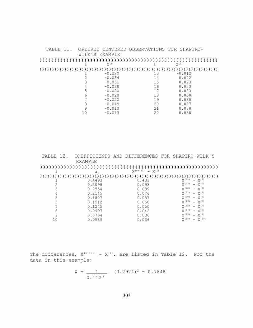
307

TABLE 11. ORDERED CENTERED OBSERVATIONS FOR SHAPIRO- WILK'S EXAMPLE

)))))))))))))))))))))))))))))))))))))))))))))))))))))))))))) i X(i) i X(i)

)))))))))))))))))))))))))))))))))))))))))))))))))))))))))))))))))))))))) 1 -0.220 13 -0.012 2 -0.054 14 0.002 3 -0.051 15 0.023 4 -0.038 16 0.023 5 -0.020 17 0.023 6 -0.020 18 0.030 7 -0.020 19 0.030 8 -0.019 20 0.037 9 -0.013 21 0.038 10 -0.013 22 0.038

TABLE 12. COEFFICIENTS AND DIFFERENCES FOR SHAPIRO-WILK'S EXAMPLE

)))))))))))))))))))))))))))))))))))))))))))))))))))))))))))) i ai X(n-i+1) - X(i)

)))))))))))))))))))))))))))))))))))))))))))))))))))))))))))))))))))))))) 1 0.4493 0.433 X(24) - X(1)

2 0.3098 0.098 X(23) - X(2)

3 0.2554 0.089 X(22) - X(3)

4 0.2145 0.076 X(21) - X(4)

5 0.1807 0.057 X(20) - X(5)

6 0.1512 0.050 X(19) - X(6)

7 0.1245 0.050 X(18) - X(7)

8 0.0997 0.042 X(17) - X(8)

9 0.0764 0.036 X(16) - X(9)

10 0.0539 0.036 X(15) - X(10)

The differences, X(n-i+1) - X(i), are listed in Table 12. For thedata in this example:

W = 1 (0.2974)2 = 0.7848 0.1127

308

14.13.2.5.7 The decision rule for this test is to compare W ascalculated in 14.13.2.5.6 to a critical value found in Table 6,Appendix B. If the computed W is less than the critical value,conclude that the data are not normally distributed. For thedata in this example, the critical value at a significance levelof 0.01 and n = 24 observations is 0.884. Since W = 0.7848 isless than the critical value, conclude that the data are notnormally distributed.

14.13.2.5.8 Since the data do not meet the assumption ofnormality, the Wilcoxon Rank Sum Test with the BonferroniAdjustment will be used to analyze the shell development data.

14.13.2.6 Wilcoxon Rank Sum Test with the Bonferroni Adjustment

14.13.2.6.1 For each control and concentration combination,combine the data and arrange the observations in order of sizefrom smallest to largest. Assign the ranks (1, 2, ... , 9) tothe ordered observations with a rank of 1 assigned to thesmallest observation, rank of 2 assigned to the next largerobservation, etc. If ties occur when ranking, assign the averagerank to each tied observation. 14.13.2.6.2 An example of assigning ranks to the combined datafor the control and 0.56% concentration is given in Table 13. This ranking procedure is repeated for each control/concentrationcombination. The complete set of rankings is summarized inTable 14. The ranks are then summed for each concentrationlevel, as shown in Table 15.

14.13.2.6.3 For this example, determine if the survival in anyof the concentrations is significantly lower than the survival inthe control. If this occurs, the rank sum at that concentrationwould be significantly lower than the rank sum of the control. Thus compare the rank sums for the survival at each of thevarious concentration levels with some "minimum" or critical ranksum, at or below which the survival would be consideredsignificantly lower than the control. At a significance level of0.05, the minimum rank sum in a test with four concentrations(excluding the control), four control replicates and fiveconcentration replicates is 15 (See Table 5, Appendix F).

309

TABLE 13. ASSIGNING RANKS TO THE CONTROL AND 0.56%CONCENTRATION LEVEL FOR THE WILCOXON RANK SUMTEST WITH THE BONFERRONI ADJUSTMENT

))))))))))))))))))))))))))))))))))))))))))))))))))))))))))))) Transformed Proportion Rank Normal Concentration )))))))))))))))))))))))))))))))))))))))))))))))))))))))))))))))))) 1 1.429 0.56 % 4 1.471 0.56 % 4 1.471 0.56 % 4 1.471 Control 4 1.471 Control 4 1.471 Control 8 1.521 0.56 % 8 1.521 0.56 % 8 1.521 Control ))))))))))))))))))))))))))))))))))))))))))))))))))))))))))))))))))

TABLE 14. TABLE OF RANKS1

))))))))))))))))))))))))))))))))))))))))))))))))))))))))))))) Effluent Concentration (%)Repli- )))))))))))))))))))))))))))))))))))))))))))))) cate Control 0.56 1.00 1.80 3.20))))))))))))))))))))))))))))))))))))))))))))))))))))))))))))))))))))))))))

1 1.471(4,3.5,5.5,7) 1.471(4) 1.471(3.5) 1.471(5.5) 0.674(1) 2 1.471(4,3.5,5.5,7) 1.471(4) 1.521(8) 1.471(5.5) 0.856(2) 3 1.471(4,3.5,5.5,7) 1.429(1) 1.471(3.5) 1.471(5.5) 0.896(3) 4 1.521(8,8,9,9) 1.521(8) 1.471(3.5) 1.429(2) 0.938(4) 5 1.521(8) 1.521(8) 1.397(1) 1.107(5)

))))))))))))))))))))))))))))))))))))))))))))))))))))))))))))))))))))))))))1Control ranks are given in the order of the concentration with which they were ranked.

310

TABLE 15. RANK SUMS ))))))))))))))))))))))))))))))))))))))))))))))))))))))))) Concentration (% Effluent) Rank Sum ))))))))))))))))))))))))))))))))))))))))))))))))))))))))) 0.56 25.0 1.00 26.5 1.80 19.5 3.20 15.0

14.13.2.6.4 Since the rank sum for the 3.20% concentration levelis equal to the critical value, the proportion normal in thatconcentration is considered significantly less than that in thecontrol. Since no other rank sum is less than or equal to thecritical value, no other concentration has a significantly lowerproportion normal than the control. Hence, the NOEC and the LOECare 1.80% and 3.20%, respectively.

14.13.2.7 Calculation of the ICp

14.13.2.7.1 The shell development data in Table 4 are utilizedin this example. As can be seen from Table 4 and Figure 4, theobserved means are not monotonically non-increasing with respectto concentration (mean response for each higher concentration isnot less than or equal to the mean response for the previousconcentration and the responses between concentrations do notfollow a linear trends). Therefore, the means are smoothed priorto calculating the IC. In the following discussion, the observedmeans are represented by Y&i and the smoothed means by Mi.

14.13.2.7.2 Starting with the control mean, Y&1 = 0.993 and Y&2 =0.992, we see that Y&1 > Y&2. Set M1 = Y&1. Comparing Y&2 to Y&3,Y&2< Y&3.

14.13.2.7.3 Calculate the smoothed means:

M2 = M3 = (Y&2 + Y&3)/2 = 0.993

14.13.2.7.4 Since Y&7 = 0 < Y&6 = 0 < Y&5 = 0.604 < Y&4 = 0.984 < Y&3

= 0.993, set M3 = 0.993, M4 = 0.984, M5 = 0.604, M6 = 0, and set M7= 0.

311

Figu

re 4

. Plo

t of r

aw d

ata,

obs

erve

d m

eans

, and

sm

ooth

ed m

eans

for r

ed

abal

one,

Hal

iotu

s ru

fesc

ens,

deve

lopm

ent d

ata

from

Tab

les

4 an

d 16

.

312

TABLE 16. RED ABALONE, HALIOTUS RUFESCENS, MEAN SHELL DEVELOPMENT RESPONSE AFTER SMOOTHING

Effluent Conc. (%) i

Response Means, Y&i (proportion)

Smoothed Means, Mi (proportion)

Control 0.56 1.00 1.80 3.20 5.60 10.00

1234567

0.993 0.992 0.994 0.984 0.604 0.000 0.000

0.993 0.993 0.993 0.984 0.604 0.000

0.000

14.13.2.7.5 Table 16 contains the response means and smoothedmeans and Figure 4 gives a plot of the smoothed response curve.

14.13.2.7.6 An IC25 can be estimated using the Linear Interpolation Method. A 25% reduction in mean proportion offertilized eggs, compared to the controls, would result in a meanproportion of 0.745, where M1(1-p/100) = 0.993(1-25/100). Examining the means and their associated concentrations(Table 16), the response, 0.745, is bracketed by C4 = 1.80%effluent and C5 = 3.20% effluent.

14.13.2.7.7 Using the equation from Section 4.2 in Appendix L,the estimate of the IC25 is calculated as follows:

ICp ' Cj%[M1(1&p/100)&Mj](C(j%1)&Cj)

(M(j%1)&Mj)

IC25 = 1.8 + [0.993(1 - 25/100) - 0.984] (3.2 - 1.8) S))))))))))))Q (0.604 - 0.984) = 2.68%.

14.13.2.7.8 When the ICPIN program was used to analyze this setof data, requesting 80 resamples, the estimate of the IC25 was2.6818%. The empirical 95.0% confidence interval for the true

313

mean was 2.5000% to 3.1262 %. The computer program output forthe IC25 for this data set is shown in Figure 5.

14.14 PRECISION AND ACCURACY

14.14.1 PRECISION

14.14.1.1 Single-Laboratory Precision

14.14.1.1.1 Data on the single laboratory precision of theHaliotis rufescens larval development method using zinc sulfateare shown in Table 17. Zinc concentrations were 18, 32, 56, and100 µg/L. All tests were conducted at the Marine PollutionStudies Laboratory. There was good agreement among test EC50s,with a coefficient of variation of 8%.

14.14.1.2 Multi-laboratory Precision

14.14.1.2.1 The multi-laboratory data indicate a similar levelof test precision Table 18. Data are presented for fourinterlaboratory trials in which either two or three laboratoriestested both split effluent samples and reference toxicants. Themean coefficient of variation between EC50 values from differentlaboratories was 15%.

14.14.2 ACCURACY

14.14.2.1 The accuracy of toxicity tests cannot be determined.

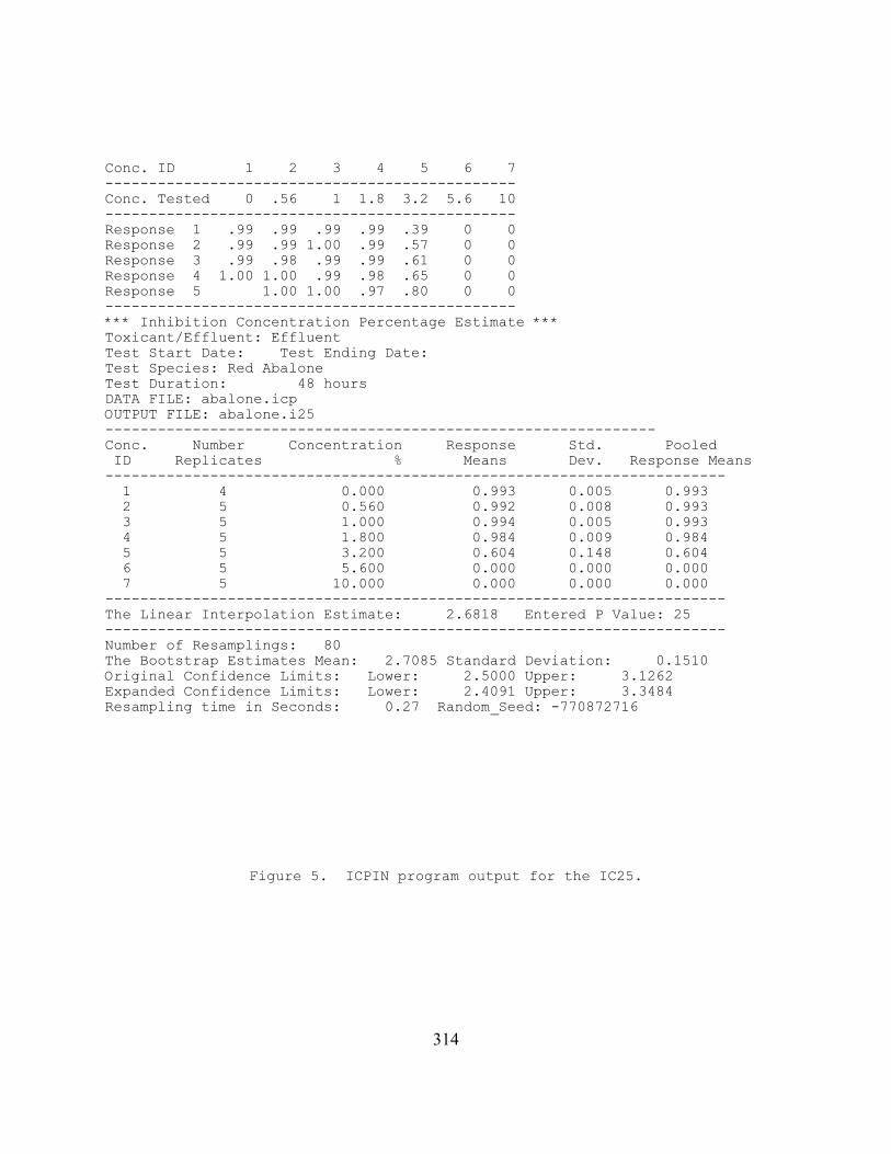
314

Conc. ID 1 2 3 4 5 6 7-----------------------------------------------Conc. Tested 0 .56 1 1.8 3.2 5.6 10-----------------------------------------------Response 1 .99 .99 .99 .99 .39 0 0Response 2 .99 .99 1.00 .99 .57 0 0Response 3 .99 .98 .99 .99 .61 0 0Response 4 1.00 1.00 .99 .98 .65 0 0Response 5 1.00 1.00 .97 .80 0 0-----------------------------------------------*** Inhibition Concentration Percentage Estimate ***Toxicant/Effluent: EffluentTest Start Date: Test Ending Date: Test Species: Red AbaloneTest Duration: 48 hoursDATA FILE: abalone.icpOUTPUT FILE: abalone.i25---------------------------------------------------------------Conc. Number Concentration Response Std. Pooled ID Replicates % Means Dev. Response Means----------------------------------------------------------------------- 1 4 0.000 0.993 0.005 0.993 2 5 0.560 0.992 0.008 0.993 3 5 1.000 0.994 0.005 0.993 4 5 1.800 0.984 0.009 0.984 5 5 3.200 0.604 0.148 0.604 6 5 5.600 0.000 0.000 0.000 7 5 10.000 0.000 0.000 0.000-----------------------------------------------------------------------The Linear Interpolation Estimate: 2.6818 Entered P Value: 25-----------------------------------------------------------------------Number of Resamplings: 80The Bootstrap Estimates Mean: 2.7085 Standard Deviation: 0.1510Original Confidence Limits: Lower: 2.5000 Upper: 3.1262Expanded Confidence Limits: Lower: 2.4091 Upper: 3.3484Resampling time in Seconds: 0.27 Random_Seed: -770872716

Figure 5. ICPIN program output for the IC25.

315

TABLE 17. SINGLE LABORATORY PRECISION DATA FOR THE RED ABALONE,HALIOTIS RUFESCENS LARVAL DEVELOPMENT TEST WITH ZINC(ZN FG/L) SULFATE AS A REFERENCE TOXICANT

Test Date NOEC (µg/L) EC50 (µg/L)

March 1990 32 421

May 1990 32 391

January 1991 18 341

February 1991 18 402

Mean 38.4

SD 3.0

CV (%) 7.8

1 Source: Hunt et al., 19912 Source: Anderson et al., 1994

316

TABLE 18. MULTI-LABORATORY PRECISION OF THE RED ABALONE, HALIOTISRUFESCENS LARVAL DEVELOPMENT TEST PERFORMED WITH ZINC(ZN FG/L) SULFATE AND EFFLUENT (%) AS THE TOXICANTS

Test Date Toxicant Lab NOEC EC50 CV

March 1990 Effluent A >3.2% nc

March 1990 Effluent B >3.2% nc

March 1990 Effluent C 0.32% 1.83 nc

March 1990 Zinc A 32 41

March 1990 Zinc B 18 28

March 1990 Zinc C 18 31 20%

May 1990 Effluent A 3.2% 4.7

May 1990 Effluent D 1.8% 3.5

May 1990 Effluent C 3.2% 3.8 16%

May 1990 Zinc A 32 39

May 1990 Zinc D 32 46

May 1990 Zinc C 32 37 12%

January1991

Effluent A <0.56% 1.5

January1991

Effluent C 1.25% 1.8 13%

January1991

Zinc A 18 34

January1991

Zinc C 32 48 24%

January1991

Effluent A 1.0% 2.7

January1991

Effluent C 1.8% 2.8 3.0%

Mean Interlaboratory CV = 15% Interlaboratory CV based on 6 tests for whichCV values could be calculated. Source: Hunt et al., 1991.

nc = indicates that the CV could not be calculated because only one laboratoryobserved a 50% effect and calculated an EC50.

317

APPENDIX I. RED ABALONE TEST: STEP-BY-STEP SUMMARY

PREPARATION OF TEST SOLUTIONS

A. Determine test concentrations and appropriate dilution waterbased on NPDES permit conditions and guidance from theappropriate regulatory agency.

B. Prepare effluent test solutions by diluting well mixedunfiltered effluent using volumetric flasks and pipettes. Use hypersaline brine where necessary to maintain all testsolutions at 34 ± 2‰. Include brine controls in tests thatuse brine.

C. Prepare a zinc reference toxicant stock solution (10,000µg/L) by adding 0.0440 g of zinc sulfate (ZnSO4N7H2O) to 1liter of reagent water.

D. Prepare zinc reference toxicant solution of 0 (control) 10,18, 32, 56 and 100 µg/L by adding 0, 1.0 1.8, 3.2, 5.6 and10.0 mL of stock solution, respectively, to a 1-L volumetricflask and filling to 1-L with dilution water.

E. Sample effluent and reference toxicant solutions forphysical/chemical analysis. Measure salinity, pH anddissolved oxygen from each test concentration.

F. Randomize numbers for test chambers and record the chambernumbers with their respective test concentrations on arandomization data sheet. Store the data sheet safely untilafter the test samples have been analyzed.

G. Place test chambers in a water bath or environmental chamberset to 15EC and allow temperature to equilibrate.

H. Measure the temperature daily in one random replicate (orseparate chamber) of each test concentration. Monitor thetemperature of the water bath or environmental chambercontinuously.

I. At the end of the test, measure salinity, pH, and dissolvedoxygen concentration from each test concentration.

318

PREPARATION AND ANALYSIS OF TEST ORGANISMS

A. Obtain test organisms and hold or condition as necessary forspawning.

B. Induce four male and four female abalone to spawn usingeither H2O2 and Tris or UV irradiated seawater (300 mL/minflow rate through the UV unit). All solutions should bemaintained at 15 ± 1EC.

C. Siphon eggs into a fertilization bucket. Add 200 mL ofsperm-laden water to fertilize the eggs. Wash thefertilized eggs at least twice by slowly decanting andrefilling the chamber with fresh filtered seawater. Temperatures should vary by no more than 1EC between watersused in mixing and refilling.

D. Suspend the embryos evenly in a 1000 mL beaker and countfive samples in a 1 mL pipet to estimate embryo density.

E. Pipet 1000 fertilized embryos into each 200 mL test chamber. Be sure temperatures in the embryo beaker and the solutionsare at 15 ± 1EC. Incubate for 48 h. For smaller-sizedchambers, use proportionately fewer embryos.

F. At the end of the 48 h period, pour the entire test solutionwith larvae through a 37 µm-meshed screen. Wash larvae fromthe screen into 25 mL vials. Add buffered formalin topreserve the larvae in a 5% solution or glutaraldehyde for a0.05% solution. Cap the flask and invert gently to mix.

G. Pipet a sample from each vial onto a Sedgwick-Raftercounting slide and count 100 larvae. Return the larvae tothe vials for future reference.

H. Count the number of normal larvae for each replicate anddivide by the total counted.

I. Analyze the data.

J. Include standard reference toxicant point estimate values inthe standard quality control charts.

319

Salinity Adjustment Worksheet for Abalone

Date Sampled: Batch:Date Adjusted: Region:

VS (TS-SS) SS = Salinity of Sample VB = Volume of Brine (SB -TS) VS = Volume of Sample SB = Salinity of Brine

TS = Target Salinity (34±2%)

VDW = VBL - VBS VDW = Volume of Dilution Water (Adjusted to 34±2%) VBL = Largest Volume of Brine added to adjust salinity

VBS = Volume of Brine added to each Sample

Total Volume = VB added + VDW added (Total volume should be the same for all samples)

Precision andAccuracy forRefractometer

Site Code (ID Org #) or concentration

Initial Salinity TS

Vol. of Brine

Vol.Dil. Water

Total Volume

Final Salinity

34±234±234±234±234±234±234±234±234±234±234±234±234±234±234±234±234±234±234±234±234±234±234±234±234±234±234±234±234±2

Initials: Double Checked:

320

Data Sheet for Mollusc Larval Development Toxicity Test

Test Start Date: Start Time: Mollusc Species:

Test End Date: End Time: Collection/Arrival Date:

ReferenceToxicant:ReferenceToxicant:

Broodstock Source:

Sample Source:

Sample Type: Effluent Ref Tox Solid Elutriate Pore Water WaterSample Type: Effluent Ref Tox Solid Elutriate Pore Water WaterTest

Cont.#

StationCode or

Concentration Sample ID #

After 48 hours

NotesNormalLarvae

AbnormalLarvae

123456789

1011121314151617181920212223242526272829303132333435

Computer Data StorageComputerData Storage

Notes

Disk:File:

321

SECTION 15

PURPLE URCHIN, Strongylocentrotus purpuratusAND SAND DOLLAR, Dendraster excentricus

LARVAL DEVELOPMENT TEST METHOD

Adapted from a method developed bySteven Bay and Darrin Greenstein

Southern California Coastal Water Research ProjectWestminster, CA 92683

TABLE OF CONTENTS

15.1 Scope and Application15.2 Summary of Method15.3 Interferences15.4 Safety15.5 Apparatus and Equipment15.6 Reagents and Supplies15.7 Effluents and Receiving Water Collection,

Preservation, and Storage15.8 Calibration and Standardization15.9 Quality Control 15.10 Test Procedures15.11 Summary of Test Conditions and Test

Acceptability Criteria15.12 Acceptability of Test Results15.13 Data Analysis15.14 Precision and Accuracy

Appendix I Step-by Step Summary

322

SECTION 15

SEA URCHIN, Strongylocentrotus purpuratusAND SAND DOLLAR, Dendraster excentricus

LARVAL DEVELOPMENT TEST

15.1 SCOPE AND APPLICATION

15.1.1 This method estimates the chronic toxicity of effluentsand receiving waters to the developing embryos of the purple seaurchin, Strongylocentrotus purpuratus, and the sand dollar,Dendraster excentricus, during a 72-h static non-renewalexposure. The effects include the synergistic, antangonistic,and additive effects of all chemical, physical, and biologicalcomponents which adversely affect the physiological andbiochemical functions of the test organisms.

15.1.2 Detection limits of the toxicity of an effluent orchemical substance are organism dependent.

15.1.3 Brief excursions in toxicity may not be detected using24-h composite samples. Also, because of the long samplecollection period involved in composite sampling and because thetest chambers are not sealed, highly volatile and highlydegradable toxicants in the source may not be detected in thetest.

15.1.4 This test is commonly used in one of two forms: (1) adefinitive test, consisting of a minimum of five effluentconcentrations and a control, and (2) a receiving water test(s),consisting of one or more receiving water concentrations and acontrol.

15.1.5 This method should be restricted to use by, or under thesupervision of, professionals experienced in aquatic toxicitytesting. Specific experience with any toxicity test is usuallyneeded before acceptable results become routine.

15.2 SUMMARY OF METHOD

15.2.1 The method provides the step-by-step instructions for

323

performing a 72-h static non-renewal test using the earlydevelopment of the purple sea urchin, Strongylocentrotuspurpuratus, and the sand dollar, Dendraster excentricus, todetermine the toxicity of substances in marine and estuarine

waters. The test endpoint is normal larval development and mayinclude mortality if modified for total counts at test initiationand termination.

15.3 INTERFERENCES

15.3.1 Toxic substances may be introduced by contaminants indilution water, glassware, sample hardware, and testing equipment(see Section 5, Facilities, Equipment, and Supplies).

15.3.2 Improper effluent sampling and handling may adverselyaffect test results (see Section 8, Effluent and Receiving WaterSampling and Sample Handling, and Sample Preparation for ToxicityTests).

15.4 SAFETY

15.4.1 See Section 3, Health and Safety

15.5 APPARATUS AND EQUIPMENT

15.5.1 Tanks, trays, or aquaria -- for holding and acclimatingadult sea urchins and sand dollars, e.g., standard salt wateraquarium or Instant Ocean Aquarium (capable of maintainingseawater at 10-20EC), with appropriate filtration and aerationsystem.

15.5.2 Air pump, air lines, and air stones -- for aerating watercontaining broodstock or for supplying air to test solutions withlow dissolved oxygen.

15.5.3 Constant temperature chambers or water baths -- formaintaining test solution temperature and keeping dilution watersupply, gametes, and embryo stock suspensions at test temperature(15EC) prior to the test.

324

15.5.4 Water purification system -- Millipore Super-Q, Deionizedwater (DI) or equivalent.

15.5.5 Refractometer -- for determining salinity.

15.5.6 Hydrometer(s) -- for calibrating refractometer.

15.5.7 Thermometers, glass or electronic, laboratory grade --for measuring water temperatures.

15.5.8 Thermometer, National Bureau of Standards Certified (seeUSEPA METHOD l70.l, USEPA, l979) -- to calibrate laboratorythermometers.

15.5.9 pH and DO meters -- for routine physical and chemicalmeasurements.

15.5.10 Standard or micro-Winkler apparatus -- for determiningDO (optional) and calibrating the DO meter.

15.5.11 Winkler bottles -- for dissolved oxygen determinations.

15.5.12 Balance -- Analytical, capable of accurately weighing to0.0001 g.

15.5.13 Fume hood -- to protect the analyst from effluent orformaldehyde fumes.

15.5.14 Glass stirring rods -- for mixing test solutions.

15.5.15 Graduated cylinders -- Class A, borosilicate glass ornon-toxic plastic labware, 50-l000 mL for making test solutions. (Note: not to be used interchangeably for gametes or embryos andtest solutions).

15.5.16 Volumetric flasks -- Class A, borosilicate glass or non-toxic plastic labware, 100-1000 mL for making test solutions.

15.5.17 Pipets, automatic -- adjustable, to cover a range ofdelivery volumes from 0.010 to 1.000 mL.

15.5.18 Pipet bulbs and fillers -- PROPIPET® or equivalent.

325

15.5.19 Wash bottles -- for reagent water, for topping offgraduated cylinders, for rinsing small glassware and instrumentelectrodes and probes.

15.5.20 Wash bottles -- for dilution water.

15.5.21 20-liter cubitainers or polycarbonate water cooler jugs-- for making hypersaline brine.

15.5.22 Cubitainers, beakers, or similar chambers of non-toxiccomposition for holding, mixing, and dispensing dilution waterand other general non-effluent, non-toxicant contact uses. Theseshould be clearly labeled and not used for other purposes.

15.5.23 Beakers, 5-10 mL borosilicate glass -- for collectingsperm from sand dollars.

15.5.24 Beakers, 250 mL borosilicate glass -- for preparation oftest solutions.

15.5.25 Beakers, 100 mL borosilicate glass -- for spawning; tosupport sea urchins and to collect sea urchin and sand dollareggs.

15.5.26 Beakers, 1,000 mL borosilicate glass -- for rinsing andsettling sea urchin eggs.

16.5.27 Vortex mixer -- to mix sea urchin semen in tubes priorto sampling.

15.5.28 Compound microscope -- for examining gametes, countingsperm cells (200-400x), eggs and embryos and (100x), andexamining larvae. Dissecting scopes are sometimes used to counteggs at a lower magnification. One piece of equipment worthy ofa special mention is an inverted microscope. The use of aninverted scope is not required, but recommended. Its use reducesthe exposure of workers to hazardous fumes (formalin orglutaraldehyde) during the counting of larvae and reduces sampleexamination time. Alternatively, a Sedgewick-Rafter cell may beused on a regular compound scope.

15.5.29 Counter, two unit, 0-999 -- for recording sperm, egg,embryo, and larval counts.

326

15.5.30 Sedgwick-Rafter counting chamber -- for counting egg andembryo stock and examining larval development at the end of thetest.

15.5.31 Centrifuge tubes, test tubes, or vials -- for holdingsemen.

15.5.32 Hemacytometers, Neubauer -- for counting sperm.

15.5.33 Siphon hose (3 mm i.d.) -- for removing wash water fromsettled eggs.

15.5.34 Perforated plunger -- for maintaining homogeneousdistribution of eggs and embryos during sampling and distributionto test chambers.

15.5.35 Enamel or plastic tray -- for optional spawningplatform.

15.5.36 Nitex® screening (0.5mm mesh) -- cleaning egg solutions.

15.5.37 60 µm NITEX® filter -- for filtering receiving waters.

15.6 REAGENTS AND SUPPLIES

15.6.1 Sample containers -- for sample shipment and storage (seeSection 8, Effluent and Receiving Water Sampling, and SampleHandling, and Sample Preparation for Toxicity Tests).

15.6.2 Data sheets (one set per test) -- for data recording (seeFigures 1-4).

15.6.3 Tape, colored -- for labelling test chambers andcontainers.

15.6.4 Markers, water-proof -- for marking containers, etc.

15.6.5 Parafilm -- to cover graduated cylinders and vesselscontaining gametes and embryos.

15.6.6 Gloves, disposable -- for personal protection fromcontamination.

327

15.6.7 Pipets, serological -- l-l0 mL, graduated.

15.6.8 Pipet tips -- for automatic pipets. Note: pipet tips forhandling semen should be cut off to produce an opening about 1 mmin diameter; pipet tips for handling eggs should be cut off toproduce an opening about 2 mm in diameter. This is necessary toprovide smooth flow of the viscous semen, accurate sampling ofeggs, and to prevent injury to eggs passing through a restrictedopening. A clean razor blade can be used to trim pipet tips.

15.6.9 Coverslips -- for microscope slides.

15.6.10 Lens paper -- for cleaning microscope optics.

15.6.11 Laboratory tissue wipes -- for cleaning and dryingelectrodes, microscope slides, etc.

15.6.12 Disposable countertop covering -- for protection of worksurfaces and minimizing spills and contamination.

15.6.13 pH buffers 4, 7, and l0 (or as per instructions ofinstrument manufacturer) -- for standards and calibration check(see USEPA Method l50.l, USEPA, l979).

15.6.14 Membranes and filling solutions -- for dissolved oxygenprobe (see USEPA Method 360.l, USEPA, l979), or reagents formodified Winkler analysis.

15.6.15 Laboratory quality assurance samples and standards --for the above methods.

15.6.16 Test chambers -- 30-mL glass scintillation vials withpolypropylene caps, four chambers per concentration.

15.6.17 Formaldehyde, 10%, in seawater -- for preserving larvae.Note: formaldehyde has been identified as a carcinogen and isirritating to skin and mucous membranes. It should not be usedat a concentration higher than necessary to achieve morphologicalpreservation of larvae for counting and only under conditions ofmaximal ventilation and minimal opportunity for volatilizationinto room air.

15.6.18 Glutaraldehyde, 1% in seawater -- for preserving larvae.

328

Figure 1. Sample experiment set-up sheet.

SEA URCHIN EMBRYO DEVELOPMENT TEST

EXPERIMENT DESCRIPTION

Bioassay No.___________ Start Date________ Start time_______

Investigator___________ End Date__________ End Time_________

SampleNumbers

Sample Concentration Other Information

329

Figure 2. Sample worksheet for urchin spawning information.

SEA URCHIN DEVELOPMENT TEST

SPAWNING WORKSHEET

Bioassay no.______________ Date ______________________

Spawning

No. Injectiontime

Sex Accepted?(Comments)

123456789101112

Sperm density

#sperm counted=__________________________________________ mean=________________________

(mean)_________ x (5 x 106)=____________ sperm/mL

Egg dilution

# eggs counted=____________________________ mean=__________________________

(mean)__________ x 100=_______________ eggs/mL in stock

eggs/mL in stock ÷ 1,000= ____________ Egg dilution factor

330

Figure 3. Sample worksheet for sea urchin fertilization information.

SEA URCHIN DEVELOPMENT TESTFERTILIZATION WORKSHEET

Bioassay No. _________________Date_______________

____________mL eggs used ______________mL dilution water used

Fertilization and initiation

__________mL in egg dilution x 1,000 eggs/mL = ____________eggs in dilution

__________eggs in dilution x 500 sperm/egg = _____________sperm needed

__________sperm needed ÷ ___________sperm/mL in spermdilution=___________mL sperm dilution needed

Percent fertilized after 10 min ____________________

Time of inoculation_____________

331

Figure 4. Sample data sheet for embryo microscopic examination.

SEA URCHIN DEVELOPMENT TEST: RESULTS

Bioassay No._______________ Date________________

Counter______________

Number Sample Abnormal Normal %Normal Notes

332

15.6.19 Acetic acid, 10%, reagent grade, in filtered (10F)seawater -- for preparing killed sperm dilutions for spermcounts.

15.6.20 Haemo-Sol or equivalent cleaner -- for cleaninghemacytometer and cover slips.

15.6.21 0.5 M KCl solution -- for inducing spawning.

15.6.22 Syringe, disposable, 3 or 5 mL -- for injecting KCl intosea urchins and sand dollars to induce spawning.

15.6.23 Needles, 25 gauge -- for injecting KCl.

15.6.24 Pasteur pipets and bulbs -- for sampling eggs fromspawning beakers.

15.6.25 Hematocrit capillary tubes -- for sampling sperm forexamination and for loading hemacytometers.

15.6.26 Microscope well-slides -- for pre-test assessment ofsperm activity and egg condition.

15.6.27 Reference toxicant solutions (see Section 15.10.2.4 andSection 4, Quality Assurance).

15.6.28 Reagent water -- defined as distilled or deionized waterthat does not contain substances which are toxic to the testorganisms (see Section 5, Facilities, Equipment, and Supplies).

15.6.29 Effluent and receiving water -- see Section 8, Effluentand Surface Water Sampling, and Sample Handling, and SamplePreparation for Toxicity Tests.

15.6.30 Dilution water and hypersaline brine -- see Section 7,Dilution Water and Section 15.6.24, Hypersaline Brines. Thedilution water should be uncontaminated 1-µm-filtered naturalseawater. Hypersaline brine should be prepared from dilutionwater.

15.6.31 HYPERSALINE BRINES

15.6.31.1 Most industrial and sewage treatment effluents

333

entering marine and estuarine systems have little measurablesalinity. Exposure of larvae to these effluents will usuallyrequire increasing the salinity of the test solutions. It isimportant to maintain an essentially constant salinity across alltreatments. In some applications it may be desirable to matchthe test salinity with that of the receiving water (See Section7.1). Two salt sources are available to adjust salinities --artificial sea salts and hypersaline brine (HSB) derived fromnatural seawater. Use of artificial sea salts is necessary onlywhen high effluent concentrations preclude salinity adjustment byHSB alone.

15.6.31.2 Hypersaline brine (HSB) can be made by concentratingnatural seawater by freezing or evaporation. HSB should be madefrom high quality, filtered seawater, and can be added to theeffluent or to reagent water to increase salinity. HSB hasseveral desirable characteristics for use in effluent toxicitytesting. Brine derived from natural seawater contains thenecessary trace metals, biogenic colloids, and some of themicrobial components necessary for adequate growth, survival,and/or reproduction of marine and estuarine organisms, and it canbe stored for prolonged periods without any apparent degradation. However, even if the maximum salinity HSB (100‰) is used as adiluent, the maximum concentration of effluent (0‰) that can be tested is 66% effluent at 34‰ salinity (see Table 1).

15.6.31.3 High quality (and preferably high salinity) seawatershould be filtered to at least 10 µm before placing into thefreezer or the brine generator. Water should be collected on anincoming tide to minimize the possibility of contamination.

15.6.31.4 Freeze Preparation of Brine

15.6.31.4.1 A convenient container for making HSB by freezing isone that has a bottom drain. One liter of brine can be made fromfour liters of seawater. Brine may be collected by partiallyfreezing seawater at -10 to -20EC until the remaining liquid hasreached the target salinity. Freeze for approximately six hours,then separate the ice (composed mainly of fresh water) from theremaining liquid (which has now become hypersaline).

334

TABLE 1. MAXIMUM EFFLUENT CONCENTRATION (%) THAT CAN BE TESTED AT 34‰ WITHOUT THE ADDITION OF DRY SALTS GIVEN THE INDICATED EFFLUENT AND BRINE SALINITIES.

Effluent Brine Brine Brine Brine Brine

Salinity‰

60‰

70‰

80‰

90‰

100‰

0 43.33 51.43 57.50 62.22 66.00

1 44.07 52.17 58.23 62.92 66.67

2 44.83 52.94 58.97 63.64 67.35

3 45.61 53.73 59.74 64.37 68.04

4 46.43 54.55 60.53 65.12 68.75

5 47.27 55.38 61.33 65.88 69.47

10 52.00 60.00 65.71 70.00 73.33

15 57.78 65.45 70.77 74.67 77.65

20 65.00 72.00 76.67 80.00 82.50

25 74.29 80.00 83.64 86.15 88.00

15.6.31.4.2 It is preferable to monitor the water until thetarget salinity is achieved rather than allowing total freezingfollowed by partial thawing. Brine salinity should never exceed100‰. It is advisable not to exceed about 70‰ brine salinityunless it is necessary to test effluent concentrations greaterthan 50%.

15.6.31.4.3 After the required salinity is attained, the HSBshould be filtered through a 1 µm filter and poured directly intoportable containers (20-L cubitainers or polycarbonate watercooler jugs are suitable). The brine storage containers shouldbe capped and labelled with the salinity and the date the brinewas generated. Containers of HSB should be stored in the dark at4EC (even room temperature has been acceptable). HSB is usuallyof acceptable quality even after several months in storage.

15.6.31.5 Heat Preparation of Brine

335

15.6.31.5.1 The ideal container for making brine using heat-assisted evaporation of natural seawater is one that (1) has ahigh surface to volume ratio, (2) is made of a non-corrosivematerial, and (3) is easily cleaned (fiberglass containers areideal). Special care should be used to prevent any toxicmaterials from coming in contact with the seawater being used togenerate the brine. If a heater is immersed directly into theseawater, ensure that the heater materials do not corrode or leach any substances that would contaminate the brine. Onesuccessful method is to use a thermostatically controlled heatexchanger made from fiberglass. If aeration is needed, use onlyoil-free air compressors to prevent contamination. 15.6.31.5.2 Before adding seawater to the brine generator,thoroughly clean the generator, aeration supply tube, heater, andany other materials that will be in direct contact with thebrine. A good quality biodegradable detergent should be used,followed by several (at least three) thorough reagent waterrinses.

15.6.31.5.3 Seawater should be filtered to at least 10 µm beforebeing put into the brine generator. The temperature of theseawater is increased slowly to 40EC. The water should beaerated to prevent temperature stratification and to increasewater evaporation. The brine should be checked daily (dependingon the volume being generated) to ensure that the salinity doesnot exceed 100‰ and that the temperature does not exceed 40EC. Additional seawater may be added to the brine to obtain thevolume of brine required.

15.6.31.5.4 After the required salinity is attained, the HSBshould be filtered through a 1 µm filter and poured directly intoportable containers (20-L cubitainers or polycarbonate watercooler jugs are suitable). The brine storage containers shouldbe capped and labelled with the salinity and the date the brinewas generated. Containers of HSB should be stored in the dark at4EC (even room temperature has been acceptable). HSB is usuallyof acceptable quality even after several months in storage.

15.6.31.6 Artificial Sea Salts

15.6.31.6.1 No data from sea urchin or sand dollar larval testsusing sea salts or artificial seawater (e.g., GP2) are available

336

for evaluation at this time, and their use must be consideredprovisional.

15.6.31.7 Dilution Water Preparation from Brine

15.6.31.7.1 Although salinity adjustment with brine is thepreferred method, the use of high salinity brines and/or reagentwater has sometimes been associated with discernible adverseeffects on test organisms. For this reason, it is recommendedthat only the minimum necessary volume of brine and reagent waterbe used to offset the low salinity of the effluent, and thatbrine controls be included in the test. The remaining dilutionwater should be natural seawater. Salinity may be adjusted inone of two ways. First, the salinity of the highest effluenttest concentration may be adjusted to an acceptable salinity, andthen serially diluted. Alternatively, each effluentconcentration can be prepared individually with appropriatevolumes of effluent and brine.

15.6.31.7.2 When HSB and reagent water are used, thoroughly mixtogether the reagent water and HSB before mixing in the effluent. Divide the salinity of the HSB by the expected test salinity todetermine the proportion of reagent water to brine. For example,if the salinity of the brine is 100‰ and the test is to beconducted at 34‰, 100‰ divided by 34‰ = 2.94. The proportion is1 part brine plus 1.94 parts reagent water. To make 1 L ofdilution water at 34‰ salinity from a HSB of 100‰, 340 mL ofbrine and 660 mL of reagent water are required. Verify thesalinity of the resulting mixture using a refractometer.

15.6.31.8 Test Solution Salinity Adjustment

15.6.31.8.1 Table 2 illustrates the preparation of testsolutions (up to 50% effluent) at 34‰ by combining effluent, HSB,and dilution water. Note: if the highest effluent concentrationdoes not exceed 50% effluent, it is convenient to prepare brineso that the sum of the effluent salinity and brine salinityequals 68‰; the required brine volume is then always equal to theeffluent volume needed for each effluent concentration as in theexample in Table 2. 15.6.31.8.2 Check the pH of all test solutions and adjust towithin 0.2 units of dilution water pH by adding, dropwise, dilute

337

hydrochloric acid or sodium hydroxide (see Section 8.8.9,Effluent and Receiving Water Sampling, Sample Handling, andSample Preparation for Toxicity Tests).

15.6.31.8.3 To calculate the amount of brine to add to eacheffluent dilution, determine the following quantities: salinityof the brine (SB, in ‰), the salinity of the effluent (SE, in ‰), and volume of the effluent to be added (VE, in mL). Then usethe following formula to calculate the volume of brine (VB, inmL) to be added:

VB = VE x (34 - SE)/(SB - 34)

15.6.31.8.4 This calculation assumes that dilution watersalinity is 34 ± 2‰.

15.6.31.9 Preparing Test Solutions

15.6.31.9.1 Ten mL of test solution are needed for each testchamber. To prepare test solutions at low effluentconcentrations (<6%), effluents may be added directly to dilutionwater. For example, to prepare 1% effluent, add 1.0 mL ofeffluent to a 100-mL volumetric flask using a volumetric pipet orcalibrated automatic pipet. Fill the volumetric flask to the100-mL mark with dilution water, stopper it, and shake to mix. Pour into a (150-250 mL) beaker and stir. Distribute equalvolumes into the replicate test chambers. The remaining testsolution can be used for chemistry.

15.6.31.9.2 To prepare a test solution at higher effluentconcentrations, hypersaline brine must usually be used. Forexample, to prepare 40% effluent, add 400 mL of effluent to a 1-liter volumetric flask. Then, assuming an effluent salinity of2‰ and a brine salinity of 66‰, add 400 mL of brine (see equationabove and Table 2) and top off the flask with dilution water. Stopper the flask and shake well. Pour into a (100-250 mL)beaker and stir. Distribute equal volumes into the replicatetest chambers. The remaining test solution can be used forchemistry.

338

TABLE 2. EXAMPLES OF EFFLUENT DILUTION SHOWING VOLUMES OFEFFLUENT (AT X‰), BRINE, AND DILUTION WATER NEEDED FORONE LITER OF EACH TEST SOLUTION.

FIRST STEP: Combine brine with reagent water or natural seawaterto achieve a brine of 68-x‰ and, unless natural seawater is usedfor dilution water, also a brine-based dilution water of 34‰.

SERIAL DILUTION:

Step 1. Prepare the highest effluent concentration to be tested by addingequal volumes of effluent and brine to the appropriate volume of dilutionwater. An example using 40% is shown.

Effluent Conc.(%)

Effluent x‰ Brine (68-x)‰

Dilution Water*34‰

40 800 mL 800 mL 400 mLStep 2. Make serial dilutions from the highest test concentration.

Effluent Conc. (%) Effluent Source Dilution Water* (34‰)

20 1000 mL of 40% 1000 mL

10 1000 mL of 20% 1000 mL

5 1000 mL of 10% 1000 mL

2.5 1000 mL of 5% 1000 mL

Control none 1000 mL

INDIVIDUAL PREPARATION:

Effluent Conc.(%)

Effluent x‰ Brine (68-x)‰ Dilution Water*34‰

40 400 mL 400 mL 200 mL

20 200 mL 200 mL 600 mL

10 100 mL 100 mL 800 mL

5 50 mL 50 mL 900 mL

2.5 25 mL 25 mL 950 mL

Control none none 1000 mL

*May be natural seawater or brine-reagent water equivalent.

339

15.6.31.10 Brine Controls

15.6.31.10.1 Use brine controls in all tests where brine isused. Brine controls contain the same volume of brine as doesthe highest effluent concentration using brine, plus the volumeof reagent water needed to reproduce the hyposalinity of theeffluent in the highest concentration, plus dilution water. Calculate the amount of reagent water to add to brine controls byrearranging the above equation, (See, 15.6.31.8.3) setting SE =0, and solving for VE.

VE = VB x (SB - 34)/(34 - SE)

If effluent salinity is essentially 0‰, the reagent water volumeneeded in the brine control will equal the effluent volume at thehighest test concentration. However, as effluent salinity andeffluent concentration increase, less reagent water volume isneeded.

15.6.32 TEST ORGANISMS, PURPLE URCHINS

15.6.32.1 Sea Urchins, Strongylocentrotus purpuratus(approximately 6 of each sex per test).

15.6.32.2 Species Identification

15.6.32.2.1 Although identification of purple sea urchins,Strogylocentrotus purpuratus, is usually a simple matter ofconfirming general body color, size, and spine appearance, thoseunfamiliar with the species should seek confirmation from localexperts.

15.6.32.3 Obtaining Broodstock

15.6.32.3.1 Adult sea urchins (Strongylocentrotus purpuratus)can be obtained from commercial suppliers or collected fromuncontaminated intertidal areas. State collection permits areusually required for collection of sea urchins and collection isprohibited or restricted in some areas. The animals are besttransported "dry," surrounded either by moist seaweed or papertowels dampened with seawater. Animals should be kept atapproximately their collection or culture temperature to preventthermal shock which can prematurely induce spawning.

340

15.6.32.4 Broodstock Culture and Handling

15.6.32.4.1 The adult sea urchins are maintained in glassaquaria or fiberglass tanks. The tanks are supplied continuously(approximately 5 L/min) with filtered natural seawater, or saltwater prepared from commericial sea salts is recirculated. Theanimals are checked daily and any obviously unhealthy animals arediscarded.

15.6.32.4.2 Although ambient temperature seawater is usuallyacceptable, maintaining sea urchins in spawning condition usuallyrequires holding at a relatively constant temperature. Theculture unit should be capable of maintaining a constanttemperature between 10 and 14EC with a water temperature controldevice.

15.6.32.4.3 Food for sea urchins -- kelp, recommended, but notnecessarily limited to, Laminaria sp., Hedophyllum sp.,Nereocystis sp., Macrocystis sp., Egregia sp., Alaria sp. orromaine lettuce. The kelp should be gathered from knownuncontaminated zones or obtained from commerical supply houseswhose kelp comes from known uncontaminated areas, or romainelettuce. Fresh food is introduced into the tanks at leastseveral times a week. Sun dried (12-24 hours) or oven dried(60EC overnight) kelp, stores well at room temperature or frozen,rehydrates well and is adequate to maintain sea urchins for longperiods. Decaying food and fecal pellets are removed asnecessary to prevent fouling.

15.6.32.4.4 Natural seawater (>30‰) is used to maintain theadult animals and ($32‰) as a control water in the tests.

15.6.32.4.5 Adult male and female (if sexes known) animals usedin field studies are transported in separate or partitionedinsulated boxes or coolers packed with wet kelp or papertoweling. Upon arrival at the field site, aquaria (or a singlepartitioned aquarium) are filled with control water, looselycovered with a styrofoam sheet and allowed to equilibrate to theholding temperature before animals are added. Healthy animalswill attach to the kelp or aquarium within hours.

15.6.32.4.6 To successfully maintain about 25 adult animals forseven days at a field site, 40-L glass aquaria using aerated,

341

recirculating, clean saline water (32‰) and a gravel bedfiltration system, are housed within a water bath, such as anINSTANT OCEANR Aquarium. The sexes should be held separately ifpossible.

15.6.33 TEST ORGANISMS, SAND DOLLARS

15.6.33.1 Sand Dollars, Dendraster excentricus, (approximately 6of each sex per test).

15.6.33.2 Species Identification

15.6.33.2.1 Although identification of sand dollars, Dendrasterexcentricus, is usually a simple matter of confirming generalbody appearance, those unfamiliar with the species should seekconfirmation from local experts.

15.6.33.3 Obtaining Broodstock 15.6.33.3.1 Adult sand dollars (Dendraster excentricus) can beobtained from commercial suppliers or collected from subtidalzones (most areas) or from intertidal zones of some shelteredwaters (e.g., Puget Sound). State collection permits may berequired for collection of sand dollars and collection prohibitedor restricted in some areas. The animals are best transported"dry," surrounded either by moist seaweed or paper towelsdampened with seawater. Animals should be kept at approximatelytheir collection or culture temperature to prevent thermal shockwhich can prematurely induce spawning.

15.6.33.4 Broodstock Culture and Handling

15.6.33.4.1 The adult sand dollars are maintained in glassaquaria or fiberglass tanks. The tanks are supplied continuously(approximately 5 L/min) with filtered natural seawater, orsaltwater prepared from commercial sea salts is recirculated. The animals are checked daily and any obviously unhealthy animalsare discarded. For longer periods than a few days, severalcentimeters or more of a sand substrate may be desirable.

15.6.33.4.2 Although ambient temperature seawater is usuallyacceptable, maintaining sand dollars in spawning conditionusually requires holding at a relatively constant temperature.

342

The culture unit should be capable of maintaining a constanttemperature between 8 and 12EC with a water temperature controldevice.

15.6.33.4.3 Sand dollars will feed on suspended or benthicmaterials such as phytoplankton, benthic diatoms, etc. Noreports of laboratory populations being maintained in spawningcondition over several years are known. It is probably mostconvenient to obtain sand dollars, use them, and then discardthem after they cease to produce good quality gametes.

15.6.33.4.4 Natural seawater (>30‰) is used to maintain theadult animals and ($32‰) as a control water in the tests.

15.6.33.4.5 Adult male and female (if sexes known) animals usedin field studies are transported in separate or partitionedinsulated boxes or coolers packed with wet kelp or papertoweling. Upon arrival at the field site, trays or aquaria (or asingle partitioned aquarium) are filled with control water,loosely covered with a styrofoam sheet and allowed to equilibrateto the holding temperature before animals are added.

15.6.33.4.6 To successfully maintain about 25 adult animals forseven days at a field site, 40-L glass aquaria using aerated,recirculating, clean saline water (>30‰) are housed within awater bath, such as an INSTANT OCEANR Aquarium. The sexes shouldbe held separately if possible.

15.7 EFFLUENT AND RECEIVING WATER COLLECTION, PRESERVATION AND STORAGE

15.7.1 See Section 8, Effluent and Receiving Water Sampling andSample Handling, and Sampling Preparation for Toxicity Tests.

15.8 CALIBRATION AND STANDARDIZATION

15.8.1 See Section 4, Quality Assurance.

15.9 QUALITY CONTROL

15.9.1 See Section 4, Quality Assurance.

15.10 TEST PROCEDURES

343

15.10.1 TEST DESIGN

15.10.1.1 The test consists of at least four replicates of fiveeffluent concentrations plus a dilution water control. Teststhat use brine to adjust salinity must also contain fourreplicates of a brine control.

15.10.1.2 Effluent concentrations are expressed as percenteffluent.

15.10.2 TEST SOLUTIONS

15.10.2.1 Receiving waters

15.10.2.1.1 The sampling point is determined by the objectivesof the test. At estuarine and marine sites, samples are usuallycollected at mid-depth. Receiving water toxicity is determinedwith samples used directly as collected or with samples passedthrough a 60 µm NITEX® filter and compared without dilution,against a control. Using four replicate chambers per test, eachcontaining 10 mL, and 400 mL for chemical analysis, would requireapproximately 440 mL of sample per test.

15.10.2.2 Effluents

15.10.2.2.1 The selection of the effluent test concentrationsshould be based on the objectives of the study. A dilutionfactor of at least 0.5 is commonly used. A dilution factor of0.5 provides hypothesis test discrimination of ± 100%, andtesting of a 16 fold range of concentrations. Hypothesis testdiscrimination shows little improvement as dilution factors areincreased beyond 0.5 and declines rapidly if smaller dilutionfactors are used. USEPA recommends that one of the five effluenttreatments must be a concentration of effluent mixed withdilution water which corresponds to the permittee's instreamwaste concentration (IWC). At least two of the effluenttreatments must be of lesser effluent concentration than the IWC,with one being at least one-half the concentration of the IWC. If 100‰ HSB is used as a diluent, the maximum concentration ofeffluent that can be tested will be 66% at 34‰ salinity.

344

15.10.2.2.2 If the effluent is known or suspected to be highlytoxic, a lower range of effluent concentrations should be used(such as 25%, 12.5%, 6.25%, 3.12% and 1.56%).

15.10.2.2.3 The volume in each test chamber is 10 mL.

15.10.2.2.4 Effluent dilutions should be prepared for allreplicates in each treatment in one container to minimizevariability among the replicates. Dispense into the appropriateeffluent test chambers.

15.10.2.3 Dilution Water

15.10.2.3.1 Dilution water should be uncontaminated 1-µm-filtered natural seawater or hypersaline brine prepared fromuncontaminated natural seawater plus reagent water (see Section7, Dilution Water). Natural seawater may be uncontaminatedreceiving water. This water is used in all dilution steps and asthe control water.

15.10.2.4 Reference Toxicant Test

15.10.2.4.1 Reference toxicant tests should be conducted asdescribed in Quality Assurance (see Section 4.7).

15.10.2.4.2 The preferred reference toxicant for sea urchins andsand dollars is copper chloride (CuCl2NH2O). Reference toxicanttests provide an indication of the sensitivity of the testorganisms and the suitability of the testing laboratory (seeSection 4 Quality Assurance). Another toxicant may be specifiedby the appropriate regulatory agency. Prepare a copper referencetoxicant stock solution (2,000 mg/L) by adding 5.366 g of copperchloride (CuCl2N2H2O) to 1 liter of reagent water. For eachreference toxicant test prepare a copper sub-stock of 3 mg/L bydiluting 1.5 mL of stock to one liter with reagent water. Alternatively, certified standard solutions can be ordered fromcommercial companies.

15.10.2.4.3 Prepare a control (0 Fg/L) plus four replicates eachof at least five consecutive copper reference toxicant solutions(e.g., from the series 3.0, 4.4, 6.5, 9.5, 13.9, 20.4, and 30.0Fg/L, by adding 0.10, 0.15, 0.22, 0.32, 0.46, 0.68, and 1.00 mLof sub-stock solution, respectively, to 100-L volumetric flasks

345

and filling to 100-mL with dilution water). Alternatively,certified standard solutions can be ordered from commercialcompanies. Start with control solutions and progress to thehighest concentration to minimize contamination.

15.10.2.4.4 If the effluent and reference toxicant tests are tobe run concurrently, then the tests must use embryos from thesame spawn. The tests must be handled in the same way and testsolutions delivered to the test chambers at the same time. Reference toxicant tests must be conducted at 34 ± 2‰.

15.10.3 COLLECTION OF GAMETES FOR THE TEST

15.10.3.1 Spawning Induction

15.10.3.1.1 Pour seawater into 100 mL beakers and place in 15ECbath or room. Allow to come to temperature. Select a sufficientnumber of sea urchins or sand dollars (based upon recent or pastspawning success) so that three of each sex are likely to providegametes of acceptable quantity and quality for the test. Duringoptimal spawning periods this may only require six animals, threeof each sex, when the sexes are known from prior spawning. During other periods, especially if the sex is not known, manymore animals may be required.

15.10.3.1.2 Care should be exercised when removing sea urchinsfrom holding tanks so that damage to tube-feet is minimized. Following removal, sea urchins should be placed into a containerlined with seawater-moistened paper towels to preventreattachment.

15.10.3.1.3 Place each sand dollar, oral side up, on a 100 mLbeaker filled with 15EC seawater or each sea urchin onto a cleantray covered with several layers of seawater moistened papertowels.

15.10.3.1.4 Handle sexes separately once known; this minimizesthe chance of accidental egg fertilization. Throughout the testprocess, it is best if a different worker, different pipets, etc.are used for males (semen) and females (eggs). Frequent washingof hands is a good practice.

15.10.3.1.5 Fill a 3 or 5 mL syringe with 0.5 M KCl and inject

346

0.5 mL through the soft periostomal membrane of each sea urchin(See Figure 5) or into the oral opening each sand dollar. Ifsexes are known, use a separate needle for each sex. If sexesare not known, rinse the needle with hot tap water between eachinjection. This will avoid the accidental injection of spermfrom males into females. Note the time of injection on the datasheet.

15.10.3.1.6 Spawning of sea urchins is sometimes induced byholding the injected sea urchin and gently shaking or swirling itfor several seconds. This may provide an additional physicalstimulus, or may aid in distributing the injected KCl.

15.10.3.1.7 Place the sea urchins onto the beakers or tray (oralside down). Place the sand dollars onto the beakers (oral sideup). Females will release orange (sea urchins) or purple (sanddollars) eggs and males will release cream-colored semen.

15.10.3.1.8 As gametes begin to be shed, note the time on thedata sheet and separate the sexes. Place male sand dollars withthe oral side up atop a small (5-10 mL) glass beaker filled with12EC seawater. Leave spawning sea urchin males on tray or beaker(oral side down) for semen collection. Female sand dollars andsea urchins are left to shed eggs into the 100-mL beakers.

15.10.3.1.9 If sufficient quantities of gametes are available,only collect gametes for the first 15 min after each animalstarts releasing. This helps to insure good quality gametes.As a general guideline, do not collect gametes from anyindividual for more than 30 minutes after the first injection.

15.10.3.1.10 If no spawning occurs after 5 or 10 minutes, asecond 0.5 mL injection may be tried. If animals do not producesufficient gametes following injection of 1.0 mL of KCl, theyshould probably not be reinjected as this seldom results inacquisition of good quality gametes and may result in mortalityof adult urchins.

15.10.3.1.11 Sections 15.10.4.2 and 15.10.6.4 describecollection and dilution of the sperm and eggs. While some of thegamete handling needs to be in a specific order, parts of theprocedure can be done simultaneously while waiting for gametes tosettle.

Figure 5. Showing the location and orientation used in theinjection of KCl into sea urchins to stimulate spawning.

15.10.3.2 Collection of Sperm

15.10.3.2.1 Sea urchin semen should be collected dry (directlyfrom the surface of the sea urchin), using either a Pasteurpipette or a 0.1 mL autopipette with the end of the tip cut offso that the opening is at least 2 mm. Pipette semen from eachmale into separate 1-15 mL conical test tubes, stored in an icewater bath.

15.10.3.3 Viability of Sperm

15.10.3.3.1 Early in the spawning process, place a very smallamount of sperm from each male sea urchin or sand dollar into

348

dilution water on a microscope slide (well slides work nicely). Examine the sperm for motility; use sperm from males with highsperm motility.

15.10.3.4 Pooling of Sperm

15.10.3.4.1 Pool equal quantities of semen from each of the seaurchin males that has been deemed good. If possible, 0.025 mLshould be pooled from each of those used and a total of at least0.05 mL of pooled semen should be available. Sperm collectedfrom good male sand dollars should be pooled after firstdecanting off the overlying water (the final sand dollar spermdensity usually is between 2x109 and 2x1010 sperm/mL).

15.10.3.5 Storage of Sperm

15.10.3.5.1 Cover each test tube or beaker with a cap orparafilm, as air exposure of semen may alter its pH through gasexchange and reduce the viability of the sperm. Keep spermcovered and on ice or refrigerated (<5EC). The sperm should beused within 4 h of collection.

15.10.4 PREPARATION OF SPERM DILUTION FOR USE IN THE TEST

15.10.4.1 Sperm Dilution

15.10.4.1.1 When ready to use sperm, mix by agitating the tubewith a vortex mixer. Add about 0.025 mL of semen to a 100 mLbeaker containing 50 mL of 15EC dilution water. Stir thissolution thoroughly with a Pasteur pipette. A drop of eggsolution from each female may be placed on a well slide and asmall amount of sperm solution added to test fertilization. Ifno fertilization membrane forms on eggs from any female, then newgametes should be collected. Keep the sperm dilution covered andat 15EC until ready for use. This dilution should be used tofertilize the eggs within 1.5 hours of being made.

15.10.4.2 Sperm Density Determination

15.10.4.2.1 Take 0.5 mL subsample of the sperm solution and addit to 5 mL of 10% acetic acid in a 50 mL graduated cylinder, tokill the sperm. Bring the volume to 50 mL with dilution water. Mix by inversion and place one drop of the killed sperm solution

349

onto each side of a hemocytometer. Let sperm settle for about 15minutes. Count the number of sperm in 80 small squares on eachside of the hemocytometer. If the counts for each side arewithin 80% of one another, then take the mean of those twocounts. If the counts are not that close, then refill thehemocytometer, recount and take the mean of the four counts. Usethe following equations to determine sperm density and record theresults on the spawning worksheet (Figure 2).

#sperm/mL=(dilution)(count)(hemacytometer conversion factor)(mm3/mL)number of squares counted

dilution=100conversion factor=4000mm3/mL=1000number of squares=80

Therefore:

#sperm/mL=(count)(5 x 106) (Equation 2A)

15.10.5 PREPARATION OF EGG SUSPENSION FOR USE IN THE TEST

15.10.5.1 Acceptability of Eggs

15.10.5.1.1 Place a small sample of eggs from each female in thecounting chamber and examine eggs with the microscope. Look forthe presence of significant quantities of immature or abnormalappearing eggs (germinal vesicle present, unusually large orsmall or irregularly shaped). Do not use the eggs from femaleshaving more than 10% abnormal eggs or from females whose eggs didnot fertilize during the test in Section 15.10.5.1.

15.10.5.2 Pooling of Eggs

15.10.5.2.1 Allow eggs to settle in the collection beakers. Decant some of the water from the collection beakers taking carenot to pour off many eggs. Pour the remaining sea urchin eggs

350

through the Nitex® screen (to remove fecal material and otherdebris) into a 1 liter beaker. Repeat with each of the "good"females. Bring the volume up to about 600 mL with dilutionwater. Allow the eggs to settle to the bottom again. Siphon offabout 400 mL of the overlying water and then bring back up to 600mL with dilution water. Do not allow the temperature to riseabove the 15EC test temperature; somewhat cooler temperatures forholding would be acceptable.

15.10.5.2.2 Pooled sand dollar eggs should be treated gently andno additional screening or rinsing step is recommended. Mix wellonce just before subsampling for egg stock calculations. This isbest done in a large graduated cylinder appropriate for thenumber of eggs available. Cover with parafilm and invert gentlyseveral times.

15.10.5.3 Density of Eggs

15.10.5.3.1 Using a plunger, mix the sea urchin egg suspensionwell. While continuing to mix, remove a 10 mL sample and placein a 1 liter graduated cylinder. Bring the volume up to 1 literwith dilution water. Mix this dilution well and remove a 1 mLsample to a counting cell. Count all the eggs in the 1 mLsample. Repeat the process and take the mean of the two counts. Calculate the number of eggs per mL in the stock solution usingEquation 3 and record the results.

# of eggs in count x 100= # eggs/mL in stock (Equation 3)

15.10.5.4 Dilution of Eggs

15.10.5.4.1 When using scintillation vials as the test chamber,the final concentration of eggs in the diluted stock must be 250eggs/0.25 mL, which is equal to 1,000 eggs/mL. To calculate thedilution factor for the eggs, use Equation 4. (If larger testchambers are used, the total number of eggs used will be greaterand the stock solution density may be adjusted, but the finalconcentration of eggs in the test solutions must remain 25eggs/mL).

# of eggs/mL in stock ÷ 1,000= Dilution factor (Equation 4)

15.10.5.4.2 The dilution factor must be greater than one. If

351

not, concentrate the eggs and recount (starting at Section15.4.5.3 The dilution factor minus 1 equals the number of partsof water that go with one part of eggs in the final dilution. For example: if the dilution factor were 5.3, then 4.3 parts ofwater would be used with 1 part eggs.

15.10.5.4.3 Make a dilution of the egg stock so that there ismore than enough volume to perform the bioassay.

15.10.5.5 Fertilization of Eggs

15.10.5.5.1 The recommended initial sperm to egg ratio forfertilization of the eggs is 500:1. Calculate the volume ofsperm dilution (Section 15.10.5.1) to add to the egg dilution, byusing the following equations and record the results (Figure 3).

volume of egg dilution x 1,000 eggs/mL= total # of eggs in dilution (Equation5A)

total # of eggs in dilution x 500 sperm/egg= # of sperm needed(Equation 5B)

# of sperm needed ÷ # sperm/mL in sperm dilution= mL of sperm solution(Equation 5C)

15.10.5.5.2 Add this volume of the sperm dilution to the eggdilution and mix gently with a plunger. Wait 10 min, then checkfor fertilization. If fertilization is not at least 90%, add asecond volume of the sperm dilution. Wait 10 min and recheck. If fertilization is still not 90%, then the test must berestarted with different gametes.

15.10.5.5.3 The test should be initiated within 1 hour offertilization being achieved.

15.10.6 START OF THE TEST

15.10.6.1 Prior to Beginning the Test

15.10.6.1.1 The test should begin as soon as possible, preferably within 24 h of sample collection. The maximum holdingtime following retrieval of the sample from the sampling deviceshould not exceed 36 h for off-site toxicity tests unlesspermission is granted by the permitting authority. In no case

352

should the sample be used in a test more than 72 h after samplecollection (see Section 8 Effluent and Receiving Water Sampling,Sample Handling, and Sample Preparation for Toxicity Test).

15.10.6.1.2 Just prior to test initiation (approximately 1 h),the temperature of a sufficient quantity of the sample to makethe test solutions should be adjusted to the test temperature (15± 1EC) and maintained at that temperature during the addition ofdilution water.

15.10.6.1.3 Increase the temperature of the water bath, room, orincubator to the required test temperature (15 ± 1EC).

15.10.6.1.4 Randomize the placement of test chambers in thetemperature-controlled water bath, room, or incubator at thebeginning of the test, using a position chart. Assign numbersfor the position of each test chamber using a random numbers orsimilar process (see Appendix A, for an example ofrandomization). Maintain the chambers in this configurationthroughout the test, using a position chart. Record thesenumbers on a separate data sheet together with the concentrationand replicate numbers to which they correspond. Identify thissheet with the date, test organism, test number, laboratory, andinvestigator's name, and safely store it away until after the seaurchins or sand dollars have been examined at the end of thetest.

15.10.6.1.5 Note: Loss of the randomization sheet wouldinvalidate the test by making it impossible to analyze the data afterwards. Make a copy of the randomization sheet and storeseparately. Take care to follow the numbering system exactlywhile filling chambers with the test solutions.

15.10.6.1.6 Arrange the test chambers randomly in the water bathor controlled temperature room. Once chambers have been labeledrandomly and filled with test solutions, they can be arranged innumerical order for convenience, since this will also ensurerandom placement of treatments.

15.10.6.1.6 If mortality is to be included as an endpoint, atleast 5 extra control chambers should be set up and identified onthe randomization sheet as initial count chambers.

353

15.10.6.2 Delivery of Fertilized Eggs

15.10.6.2.1 Gently mix the solution of fertilized eggs. Deliver0.25 mL of egg solution to each vial, using an automatic pipettewith the tip cut off to provide at least a 0.5 mm opening. Deliver the embryos into the test chambers directly from thepipette, taking care not to touch the pipette to the testsolution. The egg solution temperature must be within 1EC of thetest solutions. Keep the eggs well mixed during the deliveryprocedure.

15.10.6.3 Incubation

15.10.6.3.1 The embryos are incubated for 72 hours in the testchambers at 15 ± 1EC at ambient light level.

15.10.6.3.2 The optional extra control chambers for initialcounts should be counted as soon as possible after testinitiation. If they are sampled and counted in a non-destructivemanner they may be returned to the test but used only as a checkfor larval developmental rate. They must not be used for forroutine control counts at the end of the test.

15.10.7 LIGHT, PHOTOPERIOD, SALINITY AND TEMPERATURE

15.10.7.1 The light quality and intensity should be at ambientlaboratory conditions. Light intensity should be 10-20 µE/m2/s,or 50 to 100 foot candles (ft-c), with a 16 h light and 8 h darkcycle.

15.10.7.2 The water temperature in the test chambers should bemaintained at 15 ± 1EC. If a water bath is used to maintain thetest temperature, the water depth surrounding the test cupsshould be as deep as possible without floating the chambers.

15.10.7.3 The test salinity should be in the range of 34 ± 2‰. The salinity should vary by no more than ±2‰ among the chamberson a given day. If effluent and receiving water tests areconducted concurrently, the salinities of these tests should besimilar.

15.10.7.4 Rooms or incubators with high volume ventilationshould be used with caution because the volatilization of the

354

test solutions and evaporation of dilution water may cause widefluctuations in salinity. Covering the test chambers with cleanpolyethylene plastic may help prevent volatilization andevaporation of the test solutions.

15.10.8 DISSOLVED OXYGEN (DO) CONCENTRATION

15.10.8.1 Aeration may affect the toxicity of effluent andshould be used only as a last resort to maintain a satisfactoryDO. The DO concentration should be measured on new solutions atthe start of the test (Day 0). The DO should not fall below 4.0mg/L (see Section 8, Effluent and Receiving Water Sampling,Sample Handling, and Sample Preparation for Toxicity Tests). Ifit is necessary to aerate, all treatments and the control shouldbe aerated. The aeration rate should not exceed that necessaryto maintain a minimum acceptable DO and under no circumstancesshould it exceed 100 bubbles/minute, using a pipet with a 1-2 mmorifice, such as a 1 mL KIMAX® serological pipet No. 37033, orequivalent.

15.10.9 OBSERVATIONS DURING THE TEST

15.10.9.1 Routine Chemical and Physical Observations

15.10.9.1.1 The DO should be measured in each test solution atthe beginning of the exposure period.

15.10.9.1.2 The temperature, pH, and salinity should be measuredin all each test solution at the beginning of the exposureperiod. Temperature should also be monitored continuously orobserved and recorded daily for at least two locations in theenvironmental control system or the samples. Temperature shouldbe measured in a sufficient number of test chambers at the end ofthe test to determine temperature variation in the environmentalchamber.

15.10.9.1.3 Record all the measurements on the data sheet.

15.10.9.2 Routine Biological Observations

15.10.9.2.1 Developing embryos do not need to be monitoredduring the test under normal circumstances.

355

15.10.10 TERMINATION OF THE TEST

15.10.10.1 Ending the Test

15.10.10.1.1 Record the time the test is terminated.

15.10.10.1.2 Temperature, pH, dissolved oxygen, and salinity aremeasured at the end of the exposure period in one test chamber ateach concentration and in the control(s).

15.10.10.2 Sample Preservation

15.10.10.2.1 To terminate the test, add 1.0 mL of 37%(concentrated) buffered formalin to each sample to give a finalformalin concentration of 4%. As an alternate fixative, 0.5 mLof 1.0% glutaraldehyde may be used, in each test chamber. Tightly cap and gently mix each chamber and store for laterevaluation. (If the test is performed in larger chambers, a 10mL subsample of well mixed test solution is to be taken from eachchamber and preserved).

15.10.10.3 Counting

15.10.10.3.1 It is recommended that the embryos be examinedwithin one week of preservation. Longer storage times may alsobe used, but run the risk of sample degradation due to improperpreservation. Larvae can be counted directly in thescintillation vials using an inverted microscope. If an invertedscope is not available, then samples should be loaded into aSedgewick-Rafter cell, as follows. The embryos should first beallowed to settle to the bottom of the sample chamber. All butabout 1 mL of the overlying liquid should then be removed. Allof the remaining liquid containing the embryos should then betransferred to the counting chamber. Whichever scope is used,the embryos should be examined at about 100x power. The first 100 embryos encountered are counted using a multi-unithandcounter to track normal versus abnormal larvae. Record thedata by sample number on a data sheet (Figure 4).

15.10.10.3.2 Mortality can be determined only if: (1) allsurviving larvae are counted (either in the test vials with aninverted microscope or by total transfer to a counting chamber);or (2) the test solution is stirred with a plunger and

356

quantitative subsampling is conducted followed by total larvalcounts on the subsample. The latter procedure requireshomogeneous distribution of larvae in the test solution,quantitative transfer of larvae (without adherence to transferhardware or test chambers), and accurate volume measurements. Mortality is most important to consider with point estimates(e.g., EC25) or when mortality occurs at the NOEC for normaldevelopment.

15.10.10.4 Endpoint

15.10.10.4.1 Normal Larvae

15.10.10.4.1.1 Normally developed pluteus larvae have severaldistinctive characteristics:

(1) The larvae should have a pyramid shape with a pair ofskeletal rods that extend at least half the length ofthe long axis of the larvae (Figure 6D).

(2) The gut should be differentiated into three parts(Figure 6E). If the gut appears lobed and constrictsdistally in specimens with an obstructed view (e.g.,Figure 6D), then normal gut development may beinferred.

(3) Development of post-oral arms has begun.

15.10.10.4.2 Abnormal Larvae

15.10.10.4.2.1 Larvae need only be scored as abnormal or normalto conduct the test, but the categories of abnormalities may betracked as well. Abnormal larvae should fit into one of thefollowing categories:

(1) Pathological prehatched: Embryos at the single ormulti-cell stage with the fertilization membrane stillvisible.

(2) Pathological hatched: larvae that have nofertilization membrane and demonstrate an extensive

357

degree of malformation or necrosis. Most of these larvae appear as dark balls of cells or dissociated blobs of cells.

(3) Inhibited: larvae at the blastula or gastrula stagethat have no gut differentiation or have no orunderdeveloped skeleton. These larvae appear to bedeveloping regularly, but are at a stage earlier thanattained by control organisms (e.g., Figure 6A-C).

(4) Gut abnormalities: larvae whose overall appearance isnormal, but have guts that are lacking,undifferentiated, abnormally shaped or project outsideof the larvae (exogastrulated).

(5) Skeletal abnormalities: larvae whose overallappearance is normal, but have missing spicules,extraneous spicules or rods growing in abnormaldirections. Note: Some larvae may exhibit aseparation of the rods at the apex. This may be causedby preservation and should not be termed abnormal. Since the test is started with already fertilized eggs,any unfertilized eggs that are encountered should notbe counted as either normal or abnormal, but should beignored.

15.11 SUMMARY OF TEST CONDITIONS

15.11.1 A summary of test conditions and test acceptabilitycriteria is listed in Table 3.

15.12 ACCEPTABILITY OF TEST RESULTS

15.12.1 Test results are acceptable only if all the followingrequirements are met:

(1) larval normality must be at least 80% in the controls.

(2) the minimum significant difference (%MSD) is #20%relative to the controls.

15.13 DATA ANALYSIS

15.13.1 GENERAL

15.13.1.1 Tabulate and summarize the data. Calculate the

Figure 6. Stages of sea urchin embryo development (modified from Kume andDan 1957). A. blastula; B. gastrula; C. prism; D. pluteus (frontal view); E.pluteus (lateral view). al.arm: anterior lateral arm, e: esophagus, i: intestine, st: stomach, std: stomodaeum.

359

TABLE 3. SUMMARY OF TEST CONDITIONS AND TEST ACCEPTABILITYCRITERIA FOR THE PURPLE URCHIN, STRONGYLOCENTROTUSPURPURATUS, AND SAND DOLLAR, DENDRASTER EXCENTRICUSEMBRYO DEVELOPMENT TEST WITH EFFLUENTS AND RECEIVINGWATERS

1. Test type: Static non-renewal

2. Salinity: 34 ± 2‰

3. Temperature: 15 ± 1EC

4. Light quality: Ambient laboratoryillumination

5. Light intensity: 10-20 µE/m2/s (Ambientlaboratory levels)

6. Photoperiod: 16 h light, 8 h darkness

7. Test chamber size: 30 mL

8. Test solution volume: 10 mL

9. No. replicate chambersper concentration:

4

10. Dilution water: Uncontaminated 1-µm-filterednatural seawater orhypersaline brine preparedfrom natural seawater

11. Test concentrations: Effluents: Minimum of 5 and acontrolReceiving waters: 100%receiving water and a control

12. Dilution factor: Effluents: $0.5Receiving waters: 100%receiving water and a control

13. Test duration: 72 ± 2 hr

14. Endpoint: Normal development;mortality can be included

15. Test acceptabilitycriteria:

$80% normal shell developmentin the controls; must achievea %MSD of <25%

360

16. Sampling requirements: One sample collected at testinitiation, and preferablyused within 24 h of the timeit is removed from thesampling device (see Section8, Effluent and ReceivingWater Sampling, SampleHandling, and SamplePreparation for ToxicityTests)

17. Sample volumerequired:

1 L per test

proportion of normally developed larvae for each replicate. Asample set of test data is listed in Table 4.

15.13.1.2 The statistical tests described here must be used witha knowledge of the assumptions upon which the tests arecontingent. The assistance of a statistician is recommended foranalysts who are not proficient in statistics.

15.13.1.3 The endpoints of toxicity tests using the purple seaurchin are based on the reduction in proportion of normallydeveloped larvae. The IC25 is calculated using the LinearInterpolation Method (see Section 9, Chronic Toxicity TestEndpoints and Data Analysis). LOEC and NOEC values fordevelopment are obtained using a hypothesis testing approach suchas Dunnett's Procedure (Dunnett, 1955) or Steel's Many-one RankTest (Steel, 1959; Miller, 1981) (see Section 9). Separateanalyses are performed for the estimation of the LOEC and NOECendpoints and for the estimation of the IC25. See the Appendicesfor examples of the manual computations, and examples of datainput and program output.

15.13.2 EXAMPLE OF ANALYSIS OF PURPLE SEA URCHIN,STRONGYLOCENTROTUS PURPURATUS, DEVELOPMENT DATA

15.13.2.1 Formal statistical analysis of the larval developmentdata is outlined in Figure 7. The response used in the analysisis the proportion of normally developed larvae in each test orcontrol chamber. Separate analyses are performed for theestimation of the NOEC and LOEC endpoints and for the estimationof the IC25 endpoint. Concentrations at which there are nonormally developed larvae in any of the test chambers areexcluded from statistical analysis of the NOEC and LOEC, butincluded in the estimation of the IC25.

361

TABLE 4. DATA FROM PURPLE SEA URCHIN,STRONGYLOCENTROTUS PURPURATUS, DEVELOPMENTTEST

S))))))))))))))))))))))))))))))))))))))))))))))))))))))))))))Copper No. LarvaeConcentration No. Larvae Normally Proportion(µg/L) Replicate Exposed Developed Normal )))))))))))))))))))))))))))))))))))))))))))))))))))))))))))))))))))))))))) Control A 100 87 0.87 B 100 89 0.89 C 100 81 0.81 D 101 89 0.88 E 74 62 0.84

3.2 A 110 98 0.89 B 100 82 0.82 C 100 91 0.91 D 100 83 0.83 E 100 89 0.89

5.6 A 102 86 0.84 B 100 89 0.89 C 100 85 0.85 D 107 90 0.84 E 100 85 0.85

10.0 A 100 70 0.70 B 100 71 0.71 C 100 77 0.77 D 100 74 0.74 E 100 87 0.87

18.0 A 100 7 0.07 B 100 12 0.12 C 100 14 0.14 D 100 16 0.16 E 100 10 0.10

32.0 A 101 0 0.00 B 102 0 0.00 C 100 0 0.00 D 100 0 0.00 E 100 0 0.00

362

Figure 7. Flowchart for statistical analysis of sea urchin,Strongylocentrotus purpuratus, development test.

363

D ' 'n

i'1(Xi & X )2

15.13.2.2 For the case of equal numbers of replicates across allconcentrations and the control, the evaluation of the NOEC andLOEC endpoints is made via a parametric test, Dunnett'sProcedure, or a nonparametric test, Steel's Many-one Rank Test,on the arc sine square root transformed data. Underlyingassumptions of Dunnett's Procedure, normality and homogeneity ofvariance, are formally tested. The test for normality is theShapiro-Wilk's Test, and Bartlett's Test is used to test forhomogeneity of variance. If either of these tests fails, thenonparametric test, Steel's Many-one Rank Test, is used todetermine the NOEC and LOEC endpoints. If the assumptions ofDunnett's Procedure are met, the endpoints are estimated by theparametric procedure.

15.13.2.3 If unequal numbers of replicates occur among theconcentration levels tested, there are parametric andnonparametric alternative analyses. The parametric analysis is at test with the Bonferroni adjustment (see Appendix D). TheWilcoxon Rank Sum Test with the Bonferroni adjustment is thenonparametric alternative.

15.13.2.4 Example of Analysis of Development Data

15.13.2.4.1 This example uses toxicity data from a purple seaurchin, Strongylocentrotus purpuratus, development test performedwith copper. The response of interest is the proportion ofnormally developed larvae, thus each replicate must first betransformed by the arc sine square root transformation proceduredescribed in Appendix B. The raw and transformed data, means andvariances of the transformed observations at each copperconcentration and control are listed in Table 5. The data areplotted in Figure 8. Because there is zero normal development inall five replicates of the 32.0 µg/L copper concentration, it wasnot included in the statistical analysis and is considered aqualitative development effect.

15.13.2.5 Test for Normality

15.13.2.5.1 The first step of the test for normality is tocenter the observations by subtracting the mean of allobservations within a concentration from each observation in thatconcentration. The centered observations are summarized inTable 6.

15.13.2.5.2 Calculate the denominator, D, of the statistic:

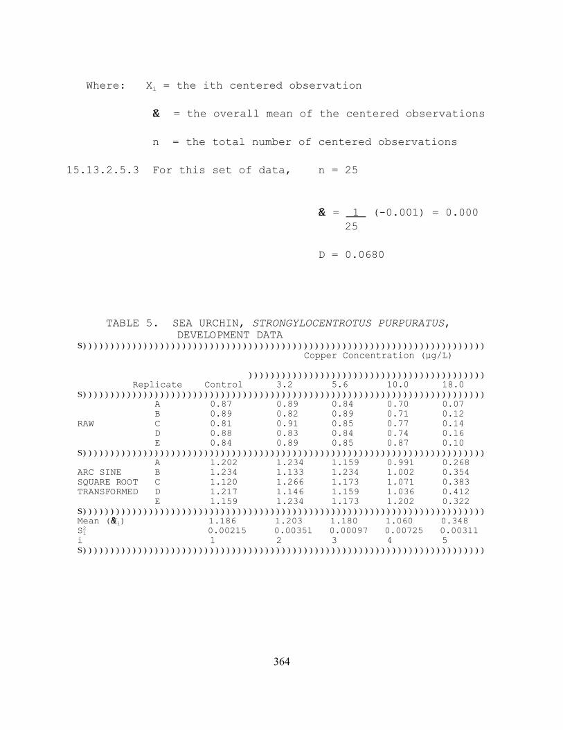
364

TABLE 5. SEA URCHIN, STRONGYLOCENTROTUS PURPURATUS, DEVELOPMENT DATA

S))))))))))))))))))))))))))))))))))))))))))))))))))))))))))))))))))))))))) Copper Concentration (µg/L)

))))))))))))))))))))))))))))))))))))))))))) Replicate Control 3.2 5.6 10.0 18.0S))))))))))))))))))))))))))))))))))))))))))))))))))))))))))))))))))))))))) A 0.87 0.89 0.84 0.70 0.07 B 0.89 0.82 0.89 0.71 0.12RAW C 0.81 0.91 0.85 0.77 0.14 D 0.88 0.83 0.84 0.74 0.16 E 0.84 0.89 0.85 0.87 0.10S))))))))))))))))))))))))))))))))))))))))))))))))))))))))))))))))))))))))) A 1.202 1.234 1.159 0.991 0.268ARC SINE B 1.234 1.133 1.234 1.002 0.354SQUARE ROOT C 1.120 1.266 1.173 1.071 0.383TRANSFORMED D 1.217 1.146 1.159 1.036 0.412 E 1.159 1.234 1.173 1.202 0.322S)))))))))))))))))))))))))))))))))))))))))))))))))))))))))))))))))))))))))Mean (Y&i) 1.186 1.203 1.180 1.060 0.348Si2 0.00215 0.00351 0.00097 0.00725 0.00311

i 1 2 3 4 5 S)))))))))))))))))))))))))))))))))))))))))))))))))))))))))))))))))))))))))

Where: Xi = the ith centered observation X& = the overall mean of the centered observations n = the total number of centered observations

15.13.2.5.3 For this set of data, n = 25

X& = 1 (-0.001) = 0.000 25

D = 0.0680

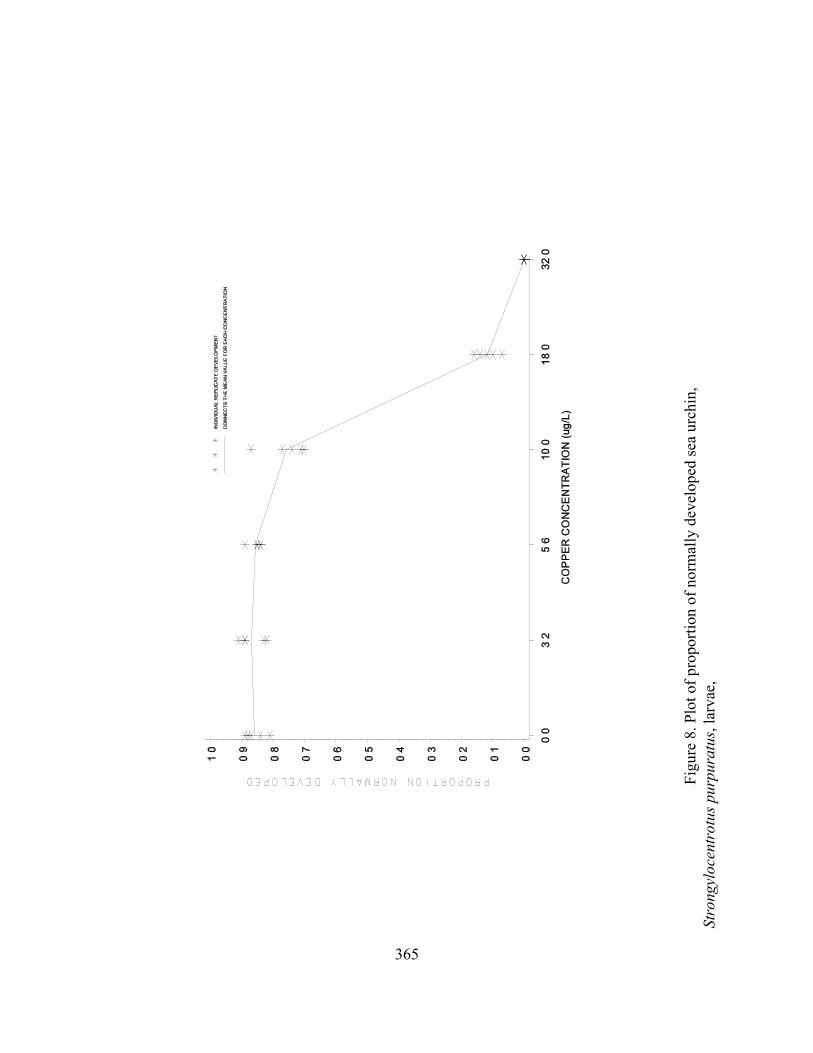
365

Figu

re 8

. Plo

t of p

ropo

rtio

n of

nor

mal

ly d

evel

oped

sea

urc

hin,

St

rong

yloc

entr

otus

pur

pura

tus,

larv

ae,

366

TABLE 6. CENTERED OBSERVATIONS FOR SHAPIRO-WILK'S EXAMPLE

S))))))))))))))))))))))))))))))))))))))))))))))))))))))))))))))))))))))))) Copper Concentration (µg/L)

S)))))))))))))))))))))))))))))))))))))))))))))))Q Replicate Control 3.2 5.6 10.0 18.0S))))))))))))))))))))))))))))))))))))))))))))))))))))))))))))))))))))))))) A 0.016 0.031 -0.021 -0.069 -0.080 B 0.048 -0.070 0.054 -0.058 0.006 C -0.066 0.063 -0.007 0.011 0.035 D 0.031 -0.057 -0.021 -0.024 0.064 E -0.027 0.031 -0.007 0.142 -0.026S)))))))))))))))))))))))))))))))))))))))))))))))))))))))))))))))))))))))))

W '1D

[ 'k

i'1ai(X

(n&i%1)&X (i))]2

15.13.2.5.4 Order the centered observations from smallest tolargest X(1) # X(2) # ... # X(n)

where X(i) denotes the ith ordered observation. The orderedobservations for this example are listed in Table 7.

15.13.2.5.5 From Table 4, Appendix B, for the number ofobservations, n, obtain the coefficients a1, a2, ... ak where k isn/2 if n is even and (n-1)/2 if n is odd. For the data in thisexample, n = 25 and k = 12. The ai values are listed in Table 8. 15.13.2.5.6 Compute the test statistic, W, as follows:

The differences, X(n-i+1) - X(i), are listed in Table 8. For thedata in this example:

W = 1 (0.2545)2 = 0.953 0.0680

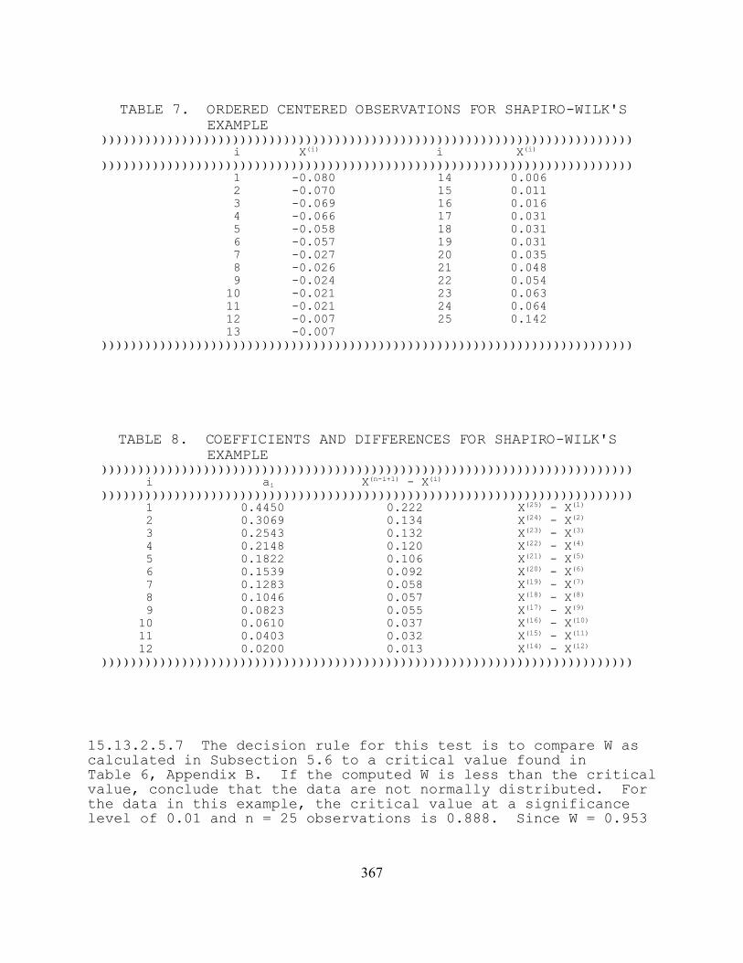
367

TABLE 7. ORDERED CENTERED OBSERVATIONS FOR SHAPIRO-WILK'S EXAMPLE

))))))))))))))))))))))))))))))))))))))))))))))))))))))))))))))))))))))))) i X(i) i X(i)

))))))))))))))))))))))))))))))))))))))))))))))))))))))))))))))))))))))))) 1 -0.080 14 0.006 2 -0.070 15 0.011 3 -0.069 16 0.016 4 -0.066 17 0.031 5 -0.058 18 0.031 6 -0.057 19 0.031 7 -0.027 20 0.035 8 -0.026 21 0.048 9 -0.024 22 0.054 10 -0.021 23 0.063 11 -0.021 24 0.064 12 -0.007 25 0.142 13 -0.007)))))))))))))))))))))))))))))))))))))))))))))))))))))))))))))))))))))))))

TABLE 8. COEFFICIENTS AND DIFFERENCES FOR SHAPIRO-WILK'S EXAMPLE

))))))))))))))))))))))))))))))))))))))))))))))))))))))))))))))))))))))))) i ai X(n-i+1) - X(i)

))))))))))))))))))))))))))))))))))))))))))))))))))))))))))))))))))))))))) 1 0.4450 0.222 X(25) - X(1)

2 0.3069 0.134 X(24) - X(2)

3 0.2543 0.132 X(23) - X(3)

4 0.2148 0.120 X(22) - X(4)

5 0.1822 0.106 X(21) - X(5)

6 0.1539 0.092 X(20) - X(6)

7 0.1283 0.058 X(19) - X(7)

8 0.1046 0.057 X(18) - X(8)

9 0.0823 0.055 X(17) - X(9)

10 0.0610 0.037 X(16) - X(10)

11 0.0403 0.032 X(15) - X(11)

12 0.0200 0.013 X(14) - X(12)

)))))))))))))))))))))))))))))))))))))))))))))))))))))))))))))))))))))))))

15.13.2.5.7 The decision rule for this test is to compare W ascalculated in Subsection 5.6 to a critical value found inTable 6, Appendix B. If the computed W is less than the criticalvalue, conclude that the data are not normally distributed. Forthe data in this example, the critical value at a significancelevel of 0.01 and n = 25 observations is 0.888. Since W = 0.953

368

B '

[( 'P

i'1Vi) ln S2 & '

P

i'1Vi ln S 2

i ]

C

S2 '

( 'P

i'1ViS

2i )

'P

i'1Vi

C ' 1% [3(p&1)]&1[ 'P

i'11/Vi& ( '

P

i'1Vi)

&1]

is greater than the critical value, conclude that the data arenormally distributed.

15.13.2.6 Test for Homogeneity of Variance

15.13.2.6.1 The test used to examine whether the variation inthe proportion of normally developed larvae is the same acrossall copper concentrations including the control, is Bartlett'sTest (Snedecor and Cochran, 1980). The test statistic is asfollows:

Where: Vi = degrees of freedom for each concentration and control,

Vi = (ni - 1)

p = number of concentration levels including the control

ni = the number of replicates for concentration i.

ln = loge

i = 1,2, ..., p where p is the number of concentrationsincluding the control

15.13.2.6.2 For the data in this example (see Table 5), allconcentrations including the control have the same number ofreplicates (ni = 5 for all i). Thus, Vi = 4 for all i.

369

B ' [(20) ln(0.00340) & 4 'Pi'1

ln(S 2i )] / 1.100

TABLE 9. ANOVA TABLE Source df Sum of Squares Mean Square(MS) (SS) (SS/df) 2 Between p - 1 SSB SB = SSB/(p-1) 2 Within N - p SSW SW = SSW/(N-p) Total N - 1 SST

15.13.2.6.3 Bartlett's statistic is, therefore:

= [20(-5.6840) - 4(-29.4325)]/1.100 = 4.050/1.100 = 3.6818 15.13.2.6.4 B is approximately distributed as chi-square withp-1 degrees of freedom, when the variances are in fact the same. Therefore, the appropriate critical value for this test, at asignificance level of 0.01 with 4 degrees of freedom, is 13.28. Since B = 3.6818 is less than the critical value of 13.28,conclude that the variances are not different. 15.13.2.7 Dunnett's Procedure

15.13.2.7.1 To obtain an estimate of the pooled variance for theDunnett's Procedure, construct an ANOVA table as described inTable 9.

Where: p = number of concentration levels including the control

N = total number of observations n1 + n2 ... + np

370

ni = number of observations in concentration i

Between Sum of SquaresSSB ' 'Pi'1

T 2i /ni&G 2/N

Total Sum of SquaresSST ' 'Pi'1'ni

j'1Y 2

ij &G 2/N

Within Sum of SquaresSSW ' SST&SSB

G = the grand total of all sample observations,G ' 'P

i'1Ti

Ti = the total of the replicate measurements forconcentration i

Yij = the jth observation for concentration i(represents the proportion of normal larvae forconcentration i in test chamber j)

15.13.2.7.2 For the data in this example:

n1 = n2 = n3 = n4 = n5 = 5

N = 25

T1 = Y11 + Y12 + Y13 + Y14 + Y15 = 5.932 T2 = Y21 + Y22 + Y23 + Y24 + Y25 = 6.013 T3 = Y31 + Y32 + Y33 + Y34 + Y35 = 5.898 T4 = Y41 + Y42 + Y43 + Y44 + Y45 = 5.302 T5 = Y51 + Y52 + Y53 + Y54 + Y55 = 1.739

G = T1 + T2 + T3 + T4 + T5 = 24.884

SSB ' 'Pi'1

T 2i /ni&G 2/N

= (137.267)/5 - (24.884)2/25 = 2.685

SST ' 'Pi'1'ni

j'1Y 2

ij &G 2/N = 27.521 - (24.884)2/25 = 2.752

= 2.752 - 2.685 = 0.067 SSW ' SST&SSB

SB2 = SSB/(p-1) = 2.685/(5-1) = 0.6713

SW2 = SSW/(N-p) = 0.067/(25-5) = 0.0034

371

TABLE 10. ANOVA TABLE FOR DUNNETT'S PROCEDURE EXAMPLE

Source df Sum of Squares Mean Square(MS) (SS) (SS/df) Between 4 2.685 0.6713

Within 20 0.067 0.0034

Total 24 2.752

ti '(Y1& Yi)

Sw (1/n1)% (1/ni)

15.13.2.7.3 Summarize these calculations in the ANOVA table(Table 10).

15.13.2.7.4 To perform the individual comparisons, calculate thet statistic for each concentration, and control combination asfollows:

Where: Y&i = mean proportion normal larvae for concentration i Y&1 = mean proportion normal larvae for the control

SW = square root of the within mean square

n1 = number of replicates for the control

ni = number of replicates for concentration i.

Since we are looking for a decreased response from the control inthe proportion of normally developed larvae, the concentrationmean is subtracted from the control mean.

372

t2 '(1.186 & 1.203)

0.0583 (1/5)% (1/5)' &0.461

TABLE 11. CALCULATED t VALUESS))))))))))))))))))))))))))))))))))))))))))))))))))))))))))))))))))))))))) Copper Concentration (µg/L) i tiS))))))))))))))))))))))))))))))))))))))))))))))))))))))))))))))))))))))))) 3.2 2 -0.461 5.6 3 0.163 10.0 4 3.417 18.0 5 22.727S)))))))))))))))))))))))))))))))))))))))))))))))))))))))))))))))))))))))))

MSD ' d Sw (1/n1)% (1/n)

15.13.2.7.5 Table 11 includes the calculated t values for eachconcentration and control combination. In this example,comparing the 3.2 µg/L copper concentration with the control thecalculation is as follows:

15.13.2.7.6 Since the purpose of this test is to detect asignificant decrease in the proportion of normally developedlarvae, a one-sided test is appropriate. The critical value forthis one-sided test is found in Table 5, Appendix C. For anoverall alpha level of 0.05, 20 degrees of freedom for error andfour concentrations (excluding the control) the critical value is2.30. The mean proportion of normally developed larvae forconcentration i is considered significantly less than the meanproportion of normally developed larvae for the control if ti isgreater than the critical value. Therefore, the 10.0 µg/L and18.0 µg/L concentrations have a significantly lower meanproportion of normally developed larvae than the control. Hencethe NOEC is 5.6 µg/L copper and the LOEC is 10.0 µg/L copper.

15.13.2.7.7 To quantify the sensitivity of the test, the minimumsignificant difference (MSD) that can be statistically detectedmay be calculated:

Where: d = the critical value for Dunnett's Procedure

SW = the square root of the within mean square

373

MSD ' 2.30 (0.0583) (1/5) % (1/5)

n = the common number of replicates at eachconcentration (this assumes equal replication ateach concentration)

n1 = the number of replicates in the control.

15.13.2.7.8 In this example,

= 2.30 (0.0583)(0.6325)

= 0.085

15.13.2.7.9 The MSD (0.085) is in transformed units. Todetermine the MSD in terms of proportion of normally developedlarvae, carry out the following conversion.

1. Subtract the MSD from the transformed control mean.

1.186 - 0.085 = 1.101

2. Obtain the untransformed values for the control mean andthe difference calculated in step 1 of 13.2.7.9.

[ Sine (1.186) ]2 = 0.859 [ Sine (1.101) ]2 = 0.795

3. The untransformed MSD (MSDu) is determined by subtractingthe untransformed values from step 2 in 14.2.7.9.

MSDu = 0.859 - 0.795 = 0.064

15.13.2.7.10 Therefore, for this set of data, the minimumdifference in mean proportion of normally developed larvaebetween the control and any copper concentration that can bedetected as statistically significant is 0.064.

15.13.2.7.11 This represents a 7.5% decrease in the proportionof normally developed larvae from the control.

15.13.2.8 Calculation of the ICp

15.13.2.8.1 The development data in Table 4 are utilized in thisexample. As can be seen from Figure 9, the observed means arenot monotonically non-increasing with respect to concentration.

374

Figu

re 9

. Plo

t of r

aw d

ata,

obs

erve

d m

eans

, and

sm

ooth

ed m

eans

for t

he s

ea

urch

in,

Stro

gylo

cent

rotu

s pu

rpur

atus

, lar

val d

evel

opm

ent d

ata

from

T

able

s 4

and

12.

375

TABLE 12. SEA URCHIN, STRONYLOCENTROTUS PURPURATUS, MEAN PROPORTION OF NORMALLY DEVELOPED LARVAE

S))))))))))))))))))))))))))))))))))))))))))))))))))))))))))))))))))))Q

Copper Response Smoothed Conc. Means, Yi Means, Mi (µg/L) i (proportion) (proportion) S))))))))))))))))))))))))))))))))))))))))))))))))))))))))))))))))))))Q Control 1 0.858 0.863 0.05 2 0.868 0.863 0.10 3 0.854 0.854 0.15 4 0.758 0.758 0.20 5 0.118 0.118 0.40 6 0.000 0.000 S))))))))))))))))))))))))))))))))))))))))))))))))))))))))))))))))))))Q

ICp ' Cj%[M1(1&p/100)&Mj](C(j%1)&Cj)

(M(j%1)&Mj)

Therefore, the means must be smoothed prior to calculating theIC.

15.13.2.8.2 Starting with the observed control mean, Y1 = 0.858,and the observed mean for the lowest copper concentration, Y2 =0.868, we see that Y1 is less than Y2.

15.13.2.8.3 Calculate the smoothed means: M1 = M2 = (Y1 + Y2)/2 = 0.863 15.13.2.8.4 Since Y3 = 0.854 > Y4 = 0.758 > Y5 = 0.118 > Y6 =0.0, set M3 = 0.854, M4 = 0.758, M5 = 0.118, and M6 = 0.0. Table 12 contains the smoothed means and Figure 8 gives a plot ofthe smoothed means and the interpolated response curve.

15.13.2.8.5 An IC25 can be estimated using the LinearInterpolation Method. A 25% reduction in mean proportion ofnormally developed larvae, compared to the controls, would resultin a mean proportion of 0.647, where M1(1-p/100) = 0.863(1-25/100). Examining the means and their associated concentrations(Table 12), the response, 0.647, is bracketed by C4 = 10.0 µg/Lcopper and C5 = 18.0 µg/L copper.

15.13.2.8.6 Using the equation from Section 4.2 in Appendix L,the estimate of the IC25 is calculated as follows:

376

Conc. ID 1 2 3 4 5 6------------------------------------------------------------------------Conc. Tested 0 3.2 5.6 10 18 32------------------------------------------------------------------------Response 1 .87 .89 .84 .70 .07 0Response 2 .89 .82 .89 .71 .12 0Response 3 .81 .91 .85 .77 .14 0Response 4 .88 .83 .84 .74 .16 0Response 5 .84 .89 .85 .87 .10 0------------------------------------------------------------------------*** Inhibition Concentration Percentage Estimate ***Toxicant/Effluent: Copper ChlorideTest Start Date: Test Ending Date: Test Species: Purple Sea Urchin, Strongylocentrotus purpuratusTest Duration: 72 hoursDATA FILE: urch_dev.icpOUTPUT FILE: urch_dev.i25-----------------------------------------------------------------------Conc. Number Concentration Response Std. Pooled ID Replicates ug/L Means Dev. Response Means----------------------------------------------------------------------- 1 5 0.000 0.858 0.033 0.863 2 5 3.200 0.868 0.040 0.863 3 5 5.600 0.854 0.021 0.854 4 5 10.000 0.758 0.068 0.758 5 5 18.000 0.118 0.035 0.118 6 5 32.000 0.000 0.000 0.000-----------------------------------------------------------------------The Linear Interpolation Estimate: 11.3844 Entered P Value: 25-----------------------------------------------------------------------Number of Resamplings: 80The Bootstrap Estimates Mean: 11.3702 Standard Deviation: 0.2898Original Confidence Limits: Lower: 10.7785 Upper: 11.9375Expanded Confidence Limits: Lower: 10.4756 Upper: 12.2141Resampling time in Seconds: 0.16 Random_Seed: 83761380

Figure 10. ICPIN program output for the IC25.

377

IC25 = 10.0 + [0.863(1 - 25/100) - 0.758] (18.0 - 10.0) S)))))))))))))Q (0.118 - 0.758) = 11.38 µg/L.

15.13.2.8.7 When the ICPIN program was used to analyze this setof data, requesting 80 resamples, the estimate of the IC25 was11.3844 µg/L. The empirical 95.0% confidence interval for thetrue mean was 10.7785 µg/L to 11.9375 µg/L. The computer programoutput for the IC25 for this data set is shown in Figure 10.

15.14 PRECISION AND ACCURACY

15.14.1 PRECISION

15.14.1.1 Single Laboratory Precision

15.14.1.1.1 Data on the single-laboratory precision of thedevelopment test using copper as a reference toxicant is providedin Table 13. The NOEC varied by only one concentration intervalindicating good precision. The coefficient of variation for theEC50 and EC25 were 22% and 21% indicating acceptable precision.

15.14.1.2 Multi-Laboratory Precision

15.14.1.2.1 Data on the multi-laboratory precision of thedevelopment test using copper as a reference toxicant is providedin Table 14. The NOEC for laboratory's A and B were identical. The difference in NOEC observed for lab C was probably due thewide range of concentrations used (See Footnote 4). Thecoefficient of variation for the EC50 was 39%, indicatingacceptable interlaboratory precision.

15.14.2 ACCURACY

15.14.2.1 The accuracy of tox1icity tests cannot be determined.

378

Table 13. SINGLE-LABORATORY PRECISION OF THE PURPLE SEA URCHIN,STRONGYLOCENTROTUS PURPURATUS, DEVELOPMENT TEST WITHCOPPER (CU µG/L) SULFATE AS A REFERENCE TOXICANT1.

Test Number NOEC (µg/L) EC50 (µg/L) EC25 (µg/L)

1 10.0 19.4 15.1

2 10.0 18.3 15.4

3 5.6 10.8 9.0

4 5.6 14.3 11.0

5 5.6 16.8 12.9

MeanCV(%)

15.9 22.0

12.7 21.0

1 Tests performed by Marine Pollution Studies Laboratory,Granite Canyon, Monterey California.

TABLE 14. MULTI-LABORATORY PRECISION OF THE PURPLE SEA URCHIN,STRONGYLOCENTROTUS PURPURATUS, DEVELOPMENT TEST WITHCOPPER (CU µG/L) SULFATE AS A REFERENCE TOXICANT.1

Lab NOEC (µg/L) EC50 (µg/L)

A2 10.0 22.5

B3 10.0 15.2

C4 1.8 10.1

MeanCV(%)

15.9 39.0

1Data from labs A and B are from an interlaboratory study using splitreference toxicant samples and dilution water. Test performed in August,1993. Test duration was 72 hr. Concentrations were 3.2, 5.6, 10, 18 and 32Fg/L.

2Test performed by Southern California Coastal Water Research Project,Westminster, CA.

3Test performed by Marine Pollution Studies Laboratory, Granite Canyon,Monterey California.4 Test performed by MEC Analytical Systems, Inc., Tiburon, CA. Testperformed in April, 1994. Test duration was 96 hr. Concentrations were 0.1,0.32, 1.8, 18 and 56 Fg/L.

379

APPENDIX I. SEA URCHIN DEVELOPMENT: STEP-BY-STEP SUMMARY

PREPARATION OF TEST SOLUTIONS

A. Determine test concentrations and appropriate dilution waterbased on NPDES permit conditions and guidance from theappropriate regulatory agency.

B. Prepare effluent test solutions by diluting well mixedunfiltered effluent using volumetric flasks and pipettes. Use hypersaline brine where necessary to maintain all testsolutions at 34 ± 2‰. Include brine controls in tests thatuse brine.

C. Prepare a copper reference toxicant stock solution.

D. Prepare a copper reference toxicant series. Add 10 mL oftest solution each vial.

E. Sample effluent and reference toxicant solutions forphysical/chemical analysis. Measure salinity, pH anddissolved oxygen of each test concentration.

F. Randomize numbers for test chambers and record the chambernumbers with their respective test concentrations on arandomization data sheet. Store the data sheet safely untilafter the test samples have been analyzed.

G. Place test chambers in a water bath or environmental chamberset to 15EC and allow temperature to equilibrate.

H. Measure the temperature daily in one random replicate (orseparate chamber) of each test concentration. Monitor thetemperature of the water bath or environmental chambercontinuously.

I. At the end of the test, measure salinity, pH, and dissolvedoxygen concentration from each test concentration.

PREPARTION AND ANALYSIS OF TEST ORGANISMS

A. Obtain test organisms and hold or condition as necessary forspawning.

B. Place six 100 mL beakers of dilution water in 15EC waterbath or room. Select 6-8 sea urchins and place on traycovered with seawater moistened paper towels. Induce

380

spawning by injecting each sea urchin with 0.5 mL of 0.5 MKCl. Place animals back onto tray, oral side down.

C. When spawning begins, note time that each animal beginsspawning. Leave males on tray for semen collection. Placespawning females oral side up on 100 mL beakers. Do notcollect gametes more than 15 min after spawning begins.

D. Collect semen using either a Pasteur pipette or a 100 FLautopipette. Pipette semen from each male into a separate 5mL conical test tube, stored in an ice water bath.

E. Check for the motility of sperm from each male.

F. Pool semen by pipetting equal amounts from each "good" maleto another centrifuge tube. At least 0.025 mL should betaken from each male and a total of at least 0.05 mL shouldbe available. Cover the tube and store in a refrigeratoruntil ready for use.

G. Finish collecting eggs before diluting semen.

H. Mix pooled semen by agitating on a vortex mixer. Add about0.025 mL of semen to a 100 mL beaker containing 50 mL of15EC dilution water. Stir thoroughly with a Pasteurpipette. Test eggs from each female to determine if theycan be fertilized.

I. Take 0.5 mL subsample of sperm dilution and add to 5 mL of10% acetic acid in a 50 mL graduated cylinder. Bring to 50mL with dilution water. Mix well by inversion and load adrop into each side of hemocytometer. Count the sperm in 80small squares. Calculate the sperm density using Equation2A.

J. Examine sample of eggs from each female. Do not use theeggs from any female whose eggs appear abnormal or that didnot fertilize in Section G.

K. Decant water from eggs of each usable female and pourthrough Nitex® screen into a 1 liter beaker. Bring volumeup to about 600 mL with dilution water. Allow to resettle,siphon about 400 mL of overlying water and bring back to 600mL with dilution water.

L. Mix egg solution well and make an accurate 100x dilutionusing at least 10 mL of the egg solution. Mix the dilutionwell and count two different 1 mL subsamples in a counting

381

cell. Use the mean of the two counts in Equation 3 todetermine the density of the egg stock.

M. Use Equation 4 to determine the egg dilution factor and makedilution of eggs with dilution water.

N. Use Equations 5 A-C to determine the volume of the spermdilution that is necessary to fertilize the egg dilution. Add the appropriate volume of sperm and after 10 minutes,check fertilization success.

O. Gently mix the fertilized egg solution with a plunger anddeliver 0.25 mL of egg solution to each vial. Make surethat the pipette tip is cut off to provide at least a 0.5 mmopening. Keep egg solution well mixed during additionperiod.

P. Incubate the embryos for 72 hours at 15 ± 1EC.

Q. Test termination and analysis

R. Perform water quality measurements as at the start.

S. After 72 hours, add 1.0 mL of 37% buffered formalin or 0.5mL of 1.0% glutaraldehyde to each test chamber. Tightly capand gently mix each vial.

T. Examine each sample with a microscope and determine thepercentage of normally developed embryos.

U. Analyze the data.

V. Include standard reference toxicant point estimate values inthe standard quality control charts.

APPENDIX II. USING THE NEUBAUER HEMACYTOMETER TO ENUMERATE SEAURCHIN SPERM

The Neubauer hemacytometer is a specialized microscope slide withtwo counting grids and a coverslip.

383

Together, the total area of each grid (1 mm2) and the verticaldistance between the grid and the coverslip (0.1 mm), providespace for a specific microvolume of aqueous sample (0.1 mm3).

This volume of liquid and the cells suspended therein (e.g.,blood cells or sperm cells) represent 1/10,000th of the liquidvolume and cell numbers of a full milliliter (cm3) of the sampledmaterial.

If the full 400-squares of each grid are counted, this representsthe number of sperm in 0.1 mm3. Multiplying this value times 10yields the sperm per mm3 (and is the source of the hemacytometerfactor of 4,000 squares/mm3). If this product is multiplied by1,000 mm3/cm3, the answer is the number of sperm in onemilliliter of the sample. If the counted sample represents adilution of a more concentrated original sample, the above answeris multiplied by the dilution factor to yield the cell density inthe original sample. If the cells are sufficiently dense, it isnot necessary to count the entire 400-square field, and the finalcalculation takes into account the number of squares actuallycounted:

cells/mL = (dilution) (4,000 squares/mm3) (1,000 mm3/cm3) (cell count) (number of squares counted)

Thus, with a dilution of 4000 (0.025 mL of semen in 100 mL ofdilution water), 80 squares counted, and a count of 100, thecalculation becomes:

cells/mL = (4,000) (4,000) (1,000) (100) 80

= 20,000,000,000 cells/mL

385

There are several procedures that are necessary for counts to beconsistent within and between laboratories. These include mixingthe sample, loading and emptying the hematocrit tube, cleaningthe hemacytometer and cover slip, and actual counting procedures.

Obviously, if the sample is not homogeneous, subsamples can varyin sperm density. A few extra seconds in mixing can save a lotof wasted minutes in subsequent counting procedures. A fullhematocrit tube empties more easily than one with just a littleliquid, so withdraw a full sample. This can be expedited bytipping the sample vial.

Because the sperm are killed prior to sampling, they will slowlysettle. For this reason, the sample in the hematocrit tubeshould be loaded onto the hemacytometer as rapidly as possible. Two replicate samples are withdrawn in fresh hematocrit tubes andloaded onto opposite sides of a hemacytometer.

386

The loaded hemacytometer is left for 15 minutes to allow thesperm to settle onto the counting field. If the coverslip ismoved after the samples are loaded, the hemacytometer should berinsed and refilled with fresh sample. After 15 minutes, thehemacytometer is placed under a microscope and the counting gridlocated at 100x. Once the grid is properly positioned, themicroscope is adjusted to 200x or 400x, and one of the cornersquares is positioned for counting (any one of the four cornersis appropriate). For consistency, use the same procedure eachtime (Many prefer to start in the upper left corner of theoptical field, and this procedure will be used in the examplesgiven below). Examine the first large square in the selectedcorner. If no sperm are visible, or if the sperm are so dense orclumped to preclude accurate counting, count a sample with a moreappropriate dilution.

In making counts of sperm, it is necessary to adopt a consistentmethod of scanning the smaller squares and counting sperm thatfall upon the lines separating the squares. Count the sperm inthe small squares by beginning in the upper left hand corner(square 1) and proceding right to square 4, down to square 5,left to square 8, etc. until all 16 squares are counted.

387

Because sperm that appear on lines might be counted as being ineither square, it is important to avoid double counting or non-counting. For this reason a convention is decided upon and usedconsistently: paraphrasing the instructions received with one(Hausser Scientific) counting chamber "to avoid counting (sperm)twice, the best practice is to count all touching the top andleft, and none touching the lower and right, boundary lines." Whatever convention is chosen, it must be adhered to. Theexample below shows a sperm count based upon a selectedconvention of counting sperm that fall on the upper and leftlines, but not on the lower or right lines:

In the above illustration, sperm falling on the lower and rightlines are not counted. The count begins at the upper left asillustrated in the preceding figure. A typical count sequence isdemonstrated by the numbers next to each sperm illustrated. Sperm identified as numbers 1, 5, 13, 20, 27, 28, 33, 51 and 54touch lines and are counted as being in the square below them orto their right. The circled sperm are not counted as being inthis field of 16 small squares (but they would be included in anycounts of adjacent squares in which they would be on upper orleft hand lines).

388

Once these counting conventions have been selected, it isadvisable to follow another strict protocol outlining the numberand sequence of large squares to be counted. Because the spermmay not be randomly distributed across the counting grid, it isrecommended to count an array of squares covering the entiregrid. The following procedure is recommended:Count the number of sperm in the first large square.

1. If the number is less than 10, count all 25 squares usingthe same scanning pattern outlined above (left to rightthrough squares 1 to 5, down to square 6, left throughsquare 10, down to 11, etc.). See pattern no. 3.

2. If the number is between 10 and 19, count 9 large squaresusing pattern no. 2.

3. If the number is 20 or greater, count 5 large squares usingpattern no. 1.

The final consideration in achieving good replicate counts iskeeping the hemacytometers and coverslips clean. They should berinsed in distilled water soon after use. The coverslips shouldbe stored in a good biocleanser such as hemasol. For an hour orso prior to use, the hemacytometer slides should also be soakedin the solution. Both slides and coverslips should then berinsed off with reagent water, blotted dry with a lint-freetissue, and wiped with lens paper.

389

SECTION 16

PURPLE URCHIN, Strongylocentrotus purpuratusAND SAND DOLLAR, Dendraster excentricus

FERTILIZATION TEST METHOD

Adapted from a method developed byGary A. Chapman, U.S. EPA, ORD Newport, OR 97365and Debra L. Denton, U.S. EPA, Region IX, CA 94105

TABLE OF CONTENTS

16.1 Scope and Application16.2 Summary of Method16.3 Interferences16.4 Safety16.5 Apparatus and Equipment16.6 Reagents and Supplies16.7 Effluents and Receiving Water Collection,

Preservation, and Storage16.8 Calibration and Standardization16.9 Quality Control 16.10 Test Procedures16.11 Summary of Test Conditions and Test

Acceptability Criteria16.12 Acceptability of Test Results16.13 Data Analysis16.14 Precision and Accuracy

Appendix I Step-by Step Summary

390

SECTION 16

SEA URCHIN, Strongylocentrotus purpuratusAND SAND DOLLAR, Dendraster excentricus

FERTILIZATION TEST

16.1 SCOPE AND APPLICATION

16.1.1 This method estimates the chronic toxicity of effluentsand receiving waters to the gametes of sea urchins,(Strongylocentrotus purpuratus), or sand dollars (Dendrasterexcentricus) during a static non-renewal 20 minute sperm exposureand a subsequent 20 minute exposure period following the additionof eggs for measuring the fertilizing capacity of the sperm. Theeffects include the synergistic, antagonistic, and additiveeffects of all chemical, physical, and biological componentswhich adversely affect the physiological and biochemicalfunctions of the test organisms.

16.1.2 The purpose of the test is to determine theconcentrations of a test substance that reduce egg fertilizationby exposed sperm relative to that attained by sperm in controlsolutions. Concentrations of materials adversely affecting eggfertilization under the conditions of this test are usuallyacutely and chronically toxic to one or more of several commonmarine test species and, by extension, are presumably acutely andchronically toxic to other of the many untested marine species.

16.1.3 Detection limits of the toxicity of an effluent orchemical substance are organism dependent.

16.1.4 Brief excursions in toxicity may not be detected using24-h composite samples. Also, because of the long samplecollection period involved in composite sampling and because thetest chambers are not sealed, highly volatile and highlydegradable toxicants in the source may not be detected in thetest.

16.1.5 This test is commonly used in one of two forms: (1) adefinitive test, consisting of a minimum of five effluentconcentrations and a control, and (2) a receiving water test(s),

391

consisting of one or more receiving water concentrations and acontrol.

16.1.6 This method should be restricted to use by, or under thesupervision of, professionals experienced in aquatic toxicitytesting. Specific experience with any toxicity test is usuallyneeded before acceptable results become routine.

16.2 SUMMARY OF METHOD

16.2.1 The method provides the step-by-step instructions forexposing sperm suspensions (appropriate sperm density may firstbe determined in a trial fertilization test) to effluents orreceiving waters for 20 minutes. Eggs are then added to thesperm suspensions and, twenty minutes after the eggs are added,the test is terminated by the addition of a preservative. Thepercent fertilization is determined by microscopic examination of100 eggs in an aliquot of eggs from each treatment. The testendpoint is normal egg fertilization.

16.3 INTERFERENCES

16.3.1 Toxic substances may be introduced by contaminants indilution water, glassware, sample hardware, and testing equipment(see Section 5, Facilities, Equipment, and Supplies).

16.3.2 Improper effluent sampling and handling may adverselyaffect test results (see Section 8, Effluent and Receiving WaterSampling and Sample Handling, and Sample Preparation for ToxicityTests).

16.4 SAFETY

16.4.1 See Section 3, Health and Safety

16.5 APPARATUS AND EQUIPMENT

16.5.1 Tanks, trays, or aquaria -- for holding and acclimatingadult sea urchins and sand dollars, e.g., standard salt wateraquarium or Instant Ocean Aquarium (capable of maintainingseawater at 10-20EC), with appropriate filtration and aerationsystem.

392

16.5.2 Air pump, air lines, and air stones -- for aerating watercontaining broodstock or for supplying air to test solutions withlow dissolved oxygen.

16.5.3 Constant temperature chambers or water baths -- formaintaining test solution temperature and keeping dilution watersupply, gametes, and embryo stock suspensions at test temperature(12EC) prior to the test. (Incubators are usually unsatisfactorybecause test tubes must be removed for addition of sperm and eggsand the small test volumes can rapidly change temperature atnormal room temperatures.)

16.5.4 Water purification system -- Millipore Super-Q, Deionizedwater (DI) or equivalent.

16.5.5 Refractometer -- for determining salinity.

16.5.6 Hydrometer(s) -- for calibrating refractometer.

16.5.7 Thermometers, glass or electronic, laboratory grade --for measuring water temperatures.

16.5.8 Thermometer, National Bureau of Standards Certified (seeUSEPA METHOD l70.l, USEPA, l979) -- to calibrate laboratorythermometers.

16.5.9 pH and DO meters -- for routine physical and chemicalmeasurements.

16.5.10 Standard or micro-Winkler apparatus -- for determiningDO (optional) and calibrating the DO meter.

16.5.11 Winkler bottles -- for dissolved oxygen determinations.

16.5.12 Balance -- Analytical, capable of accurately weighing to0.0001 g.

16.5.13 Fume hood -- to protect the analyst from effluent orformaldehyde fumes.

16.5.14 Glass stirring rods -- for mixing test solutions.

393

16.5.15 Graduated cylinders -- Class A, borosilicate glass ornon-toxic plastic labware, 50-l000 mL for making test solutions. (Note: not to be used interchangeably for gametes or embryos andtest solutions).

16.5.16 Volumetric flasks -- Class A, borosilicate glass or non-toxic plastic labware, 10-1000 mL for making test solutions.

16.5.17 Pipets, automatic -- adjustable, to cover a range ofdelivery volumes from 0.010 to 1.000 mL.

16.5.18 Pipet bulbs and fillers -- PROPIPET® or equivalent.

16.5.19 Wash bottles -- for reagent water, for topping offgraduated cylinders, for rinsing small glassware and instrumentelectrodes and probes.

16.5.20 Wash bottles -- for dilution water.

16.5.21 20-liter cubitainers or polycarbonate water cooler jugs-- for making hypersaline brine.

16.5.22 Cubitainers, beakers, or similar chambers of non-toxiccomposition for holding, mixing, and dispensing dilution waterand other general non-effluent, non-toxicant contact uses. Theseshould be clearly labeled and not used for other purposes. Strong solutions of NaOH and formaldehyde should not be held forseveral month periods in Cubitainers: interaction or leachinginto solutions of 0.1 N or 1 N NaOH used for pH adjustment ofdilution water has caused poor egg fertilization; formaldehydesimilarly stored has induced abberant partial membrane elevationin eggs.

16.5.23 Beakers, 5-10 mL borosilicate glass -- for collectingsperm from sand dollars.

16.5.24 Beakers, 100 mL borosilicate glass -- for spawning; tosupport sea urchins and to collect sea urchin and sand dollareggs.

16.5.25 Beakers, 1,000 mL borosilicate glass -- for rinsing andsettling sea urchin eggs.

394

16.5.26 Vortex mixer -- to mix sea urchin semen in tubes priorto sampling.

16.5.27 Compound microscope -- for examining gametes, countingsperm cells (200-400x) and eggs (100x), and examining fertilizedeggs. Dissecting scopes are sometimes used to count eggs at alower magnification.

16.5.28 Counter, two unit, 0-999 -- for recording sperm and eggcounts.

16.5.29 Sedgwick-Rafter counting chamber -- for counting eggstock and examining eggs for fertilization at the end of thetest.

16.5.30 Hemacytometers, Neubauer -- for counting sperm.

16.5.31 Siphon hose (3 mm i.d.) -- for removing wash water fromsettled eggs.

16.5.32 Centrifuge tubes, test tubes, or vials -- for holdingsemen.

16.5.33 Perforated plunger -- for maintaining homogeneousdistribution of eggs during sampling and distribution to testtubes.

16.5.34 60 µm NITEX® filter -- for filtering receiving water.

16.6 REAGENTS AND SUPPLIES

16.6.1 Sample containers -- for sample shipment and storage (seeSection 8, Effluent and Receiving Water Sampling, and SampleHandling, and Sample Preparation for Toxicity Tests).

16.6.2 Data sheets (one set per test) -- for data recording (seeFigures 1 and 2).

16.6.3 Tape, colored -- for labelling test chambers andcontainers.

16.6.4 Markers, water-proof -- for marking containers, etc.

395

16.6.5 Parafilm -- to cover graduated cylinders and vesselscontaining gametes.

16.6.6 Gloves, disposable -- for personal protection fromcontamination.

16.6.7 Pipets, serological -- l-l0 mL, graduated.

16.6.8 Pipet tips -- for automatic pipets. Note: pipet tips forhandling semen should be cut off to produce an opening about 1 mmin diameter; pipet tips for handling eggs should be cut off toproduce an opening about 2 mm in diameter. This is necessary toprovide smooth flow of the viscous semen, accurate sampling ofeggs, and to prevent injury to eggs passing through a restrictedopening. A clean razor blade can be used to trim pipet tips.

16.6.9 Coverslips -- for microscope slides.

16.6.10 Lens paper -- for cleaning microscope optics.

16.6.11 Laboratory tissue wipes -- for cleaning and dryingelectrodes, microscope slides, etc.

16.6.12 Disposable countertop covering -- for protection of worksurfaces and minimizing spills and contamination.

16.6.13 pH buffers 4, 7, and 10 (or as per instructions of instrument manufacturer) -- for standards and calibration check(see USEPA Method l50.l, USEPA, l979).

16.6.14 Membranes and filling solutions -- for dissolved oxygenprobe (see USEPA Method 360.l, USEPA, l979), or reagents formodified Winkler analysis.

16.6.15 Laboratory quality assurance samples and standards --for the above methods.

16.6.16 Test chambers -- test tubes, borosilicate glass, 16 x100 mm or 16 x 125 mm, with caps for conducting the test, fourchambers per concentration.

396

Figure 1. Sample data sheet for spawning record.

Animal Time No. Sex Injected Spawn Comments

1

2

3

4

5

6

7

8

9

10

11

12

Pooled eggs from female nos. .

Pooled ( mL) of sperm each from male nos. .

397

Figure 2. Sample data sheet for egg and sperm counts.

EGG COUNTS -

Sample Dilution Count Eggs/mL

For 100 mL egg suspension at 2,240 eggs/mL use:

100 mL x 2,240 eggs/mL / (counted eggs/mL) = mL of egg stock

224,000 eggs / eggs/mL = mL

If required stock >100 mL, concentrate egg stock by settling theeggs and decanting off sufficient overlying water to retain:

(________ eggs/mL / 2,240 eggs/mL) x 100 = ______ % volume

SPERM COUNTS -

Sample Dilution Count Squares Sperm/mL

SPERM/mL = (DIL.FACT.) (COUNT) (4000) (1000) (NO. SQUARES COUNTED)

398

16.6.17 Formaldehyde, 10%, in seawater -- for preserving eggs.Note: formaldehyde has been identified as a carcinogen and isirritating to skin and mucous membranes. It should not be used at a concentration higher than necessary to achieve morphologicalpreservation of larvae for counting and only under conditions ofmaximal ventilation and minimal opportunity for volatilizationinto room air.

16.6.18 Glutaraldehyde, 1% in seawater -- for preserving eggs.

16.6.13 pH buffers 4, 7, and l0 (or as per instructions of 16.6.19 Acetic acid, 10%, reagent grade, in filtered (10F)seawater -- for preparing killed sperm dilutions for spermcounts.

16.6.20 Haemo-Sol or equivalent cleaner -- for cleaninghemacytometer and cover slips.

16.6.21 0.5 M KCl solution -- for inducing spawning.

16.6.22 Syringe, disposable, 3 or 5 mL -- for injecting KCl intosea urchins and sand dollars to induce spawning.

16.6.23 Needles, 25 gauge -- for injecting KCl.

16.6.24 Pasteur pipets and bulbs -- for sampling eggs fromspawning beakers.

16.6.25 Hematocrit capillary tubes -- for sampling sperm forexamination and for loading hemacytometers.

16.6.26 Microscope well-slides -- for pre-test assessment ofsperm activity and egg condition.

16.6.27 Reference toxicant solutions (see 16.10.2.4 and Section4, Quality Assurance).

16.6.28 Reagent water -- defined as distilled or deionized waterthat does not contain substances which are toxic to the testorganisms (see Section 5, Facilities, Equipment, and Supplies andSection 7, Dilution Water).

399

16.6.29 Effluent and receiving water -- see Section 8, Effluentand Surface Water Sampling, and Sample Handling, and SamplePreparation for Toxicity Tests.

16.6.30 Dilution water and hypersaline brine -- see Section 7,Dilution Water and Section 16.6.24, Hypersaline Brines. Thedilution water should be uncontaminated 1-µm-filtered naturalseawater. Hypersaline brine should be prepared from dilutionwater.

16.6.31 HYPERSALINE BRINES

16.6.31.1 Most industrial and sewage treatment effluentsentering marine and estuarine systems have little measurablesalinity. Exposure of larvae to these effluents will usuallyrequire increasing the salinity of the test solutions. It isimportant to maintain an essentially constant salinity across alltreatments. In some applications it may be desirable to matchthe test salinity with that of the receiving water (See Section7.1). Two salt sources are available to adjust salinities --artificial sea salts and hypersaline brine (HSB) derived fromnatural seawater. Use of artificial sea salts is necessary onlywhen high effluent concentrations preclude salinity adjustment byHSB alone.

16.6.31.2 Hypersaline brine (HSB) can be made by concentratingnatural seawater by freezing or evaporation. HSB should be madefrom high quality, filtered seawater, and can be added to theeffluent or to reagent water to increase salinity. HSB hasseveral desirable characteristics for use in effluent toxicitytesting. Brine derived from natural seawater contains thenecessary trace metals, biogenic colloids, and some of themicrobial components necessary for adequate growth, survival,and/or reproduction of marine and estuarine organisms, and it canbe stored for prolonged periods without any apparent degradation. However, even if the maximum salinity HSB (100‰) is used as adiluent, the maximum concentration of effluent (0‰) that can betested is 66% effluent at 34‰ salinity (see Table 1).

16.6.31.3 High quality (and preferably high salinity) seawatershould be filtered to at least 10 µm before placing into thefreezer or the brine generator. Water should be collected on anincoming tide to minimize the possibility of contamination.

400

16.6.31.4 Freeze Preparation of Brine

16.6.31.4.1 A convenient container for making HSB by freezing isone that has a bottom drain. One liter of brine can be made fromfour liters of seawater. Brine may be collected by partiallyfreezing seawater at -10 to -20EC until the remaining liquid hasreached the target salinity. Freeze for approximately six hours,then separate the ice (composed mainly of fresh water) from theremaining liquid (which has now become hypersaline).

16.6.31.4.2 It is preferable to monitor the water until thetarget salinity is achieved rather than allowing total freezingfollowed by partial thawing. Brine salinity should never exceed100‰. It is advisable not to exceed about 70‰ brine salinityunless it is necessary to test effluent concentrations greaterthan 50%.

16.6.31.4.3 After the required salinity is attained, the HSBshould be filtered through a 1 µm filter and poured directly intoportable containers (20-L cubitainers or polycarbonate watercooler jugs are suitable). The brine storage containers shouldbe capped and labelled with the salinity and the date the brinewas generated. Containers of HSB should be stored in the dark at4EC (even room temperature has been acceptable). HSB is usuallyof acceptable quality even after several months in storage.16.6.31.5 Heat Preparation of Brine

16.6.31.5.1 The ideal container for making brine using heat-assisted evaporation of natural seawater is one that (1) has ahigh surface to volume ratio, (2) is made of a non-corrosivematerial, and (3) is easily cleaned (fiberglass containers areideal). Special care should be used to prevent any toxicmaterials from coming in contact with the seawater being used togenerate the brine. If a heater is immersed directly into theseawater, ensure that the heater materials do not corrode or leach any substances that would contaminate the brine. Onesuccessful method is to use a thermostatically controlled heatexchanger made from fiberglass. If aeration is applied, use onlyoil-free air compressors to prevent contamination. 16.6.31.5.2 Before adding seawater to the brine generator,thoroughly clean the generator, aeration supply tube, heater, andany other materials that will be in direct contact with the

401

brine. A good quality biodegradable detergent should be used,followed by several (at least three) thorough reagent waterrinses.

16.6.31.5.3 Seawater should be filtered to at least 10 µm beforebeing put into the brine generator. The temperature of theseawater is increased slowly to 40EC. The water should beaerated to prevent temperature stratification and to increasewater evaporation. The brine should be checked daily (dependingon the volume being generated) to ensure that the salinity doesnot exceed 100‰ and that the temperature does not exceed 40EC. Additional seawater may be added to the brine to obtain thevolume of brine required.

16.6.31.5.4 After the required salinity is attained, the HSBshould be filtered through a 1 µm filter and poured directly intoportable containers (20-L cubitainers or polycarbonate watercooler jugs are suitable). The brine storage containers shouldbe capped and labelled with the salinity and the date the brinewas generated. Containers of HSB should be stored in the dark at4EC (even room temperature has been acceptable). HSB is usuallyof acceptable quality even after several months in storage.

16.6.31.6 Artificial Sea Salts

16.6.31.6.1 No data from sea urchin or sand dollar fertilizationtests using sea salts are available for evaluation at this time,and their use should be considered provisional. The use of GP2artificial seawater (Table 2) has been found to provide controlfertilization equal to that of natural seawater.

16.6.31.6.2 The GP2 reagent grade chemicals (Table 2) should bemixed with deionized (DI) water or its equivalent in a singlebatch, never by test concentration or replicate. The reagentwater used for hydration should be between 21-26EC. Theartificial seawater must be conditioned (aerated) for 24 h beforeuse as the testing medium. If the solution is to be autoclaved,sodium bicarbonate is added after the solution has cooled. Astock solution of sodium bicarbonate is made up by dissolving33.6 g NaHCO3 in 500 mL of reagent water. Add 2.5 mL of thisstock solution for each liter of the GP2 artificial seawater.

16.6.31.7 Dilution Water Preparation from Brine

402

16.6.31.7.1 Although salinity adjustment with brine is thepreferred method, the use of high salinity brines and/or reagentwater has sometimes been associated with discernible adverseeffects on test organisms. For this reason, it is recommendedthat only the minimum necessary volume of brine and reagent waterbe used to offset the low salinity of the effluent, and thatbrine controls be included in the test. The remaining dilutionwater should be natural seawater. Salinity may be adjusted inone of two ways. First, the salinity of the highest effluent

test concentration may be adjusted to an acceptable salinity, andthen serially diluted. Alternatively, each effluentconcentration can be prepared individually with appropriatevolumes of effluent and brine.

16.6.31.7.2 When HSB and reagent water are used, thoroughly mixtogether the reagent water and HSB before mixing in the effluent. Divide the salinity of the HSB by the expected test salinity todetermine the proportion of reagent water to brine. For example,if the salinity of the brine is 100‰ and the test is to beconducted at 34‰, 100‰ divided by 34‰ = 2.94. Thus, theproportion is one part brine plus 1.94 parts reagent water). Tomake 1 L of dilution water at 34‰ salinity from a HSB of 100‰,340 mL of brine and 660 mL of reagent water are required. Verifythe salinity of the resulting mixture using a refractometer.

16.6.31.8 Test Solution Salinity Adjustment

16.6.31.8.1 Table 3 illustrates the preparation of testsolutions (up to 50% effluent) at 34‰ by combining effluent, HSB,and dilution water. Note: if the highest effluent concentrationdoes not exceed 50% effluent, it is convenient to prepare brineso that the sum of the effluent salinity and brine salinityequals 68‰; the required brine volume is then always equal to theeffluent volume needed for each effluent concentration as in theexample in Table 3.

16.6.31.8.2 Check the pH of all brine mixtures and adjust towithin 0.2 units of dilution water pH by adding, dropwise, dilutehydrochloric acid or sodium hydroxide.

403

TABLE 1. MAXIMUM EFFLUENT CONCENTRATION (%) THAT CAN BE TESTEDAT 34‰ WITHOUT THE ADDITION OF DRY SALTS GIVEN THEINDICATED EFFLUENT AND BRINE SALINITIES.

Effluent Brine Brine Brine Brine Brine

Salinity‰

60‰

70‰

80‰

90‰

100‰

0 43.33 51.43 57.50 62.22 66.00

1 44.07 52.17 58.23 62.92 66.67

2 44.83 52.94 58.97 63.64 67.35

3 45.61 53.73 59.74 64.37 68.04

4 46.43 54.55 60.53 65.12 68.75

5 47.27 55.38 61.33 65.88 69.47

10 52.00 60.00 65.71 70.00 73.33

15 57.78 65.45 70.77 74.67 77.65

20 65.00 72.00 76.67 80.00 82.50

25 74.29 80.00 83.64 86.15 88.00

16.6.31.8.3 To calculate the amount of brine to add to eacheffluent dilution, determine the following quantities: salinityof the brine (SB, in ‰), the salinity of the effluent (SE, in ‰), and volume of the effluent to be added (VE, in mL). Then usethe following formula to calculate the volume of brine (VB, inmL) to be added:

VB = VE x (34 - SE)/(SB - 34)

16.6.31.8.4 This calculation assumes that dilution watersalinity is 34 ± 2‰.

16.6.31.9 Preparing Test Solutions

404

TABLE 2. REAGENT GRADE CHEMICALS USED IN THE PREPARATION OF GP2ARTIFICIAL SEAWATER FOR THE PURPLE URCHINSTRONGYLOCENTROTUS PURPURATUS, AND SAND DOLLARDENDRASTER EXCENTRICUS TOXICITY TEST1,2

Compound Concentration(g/L)

Amount (g)Required for 20 L

NaCl 23.90 478.0

Na2SO4 4.00 80.0

KCl 0.698 13.96

KBr 0.100 2.00

Na2B4O7 ! 10 H2O 0.039 0.78

MgCl2 ! 6 H2O 10.80 216.0

CaCl2 ! 2 H2O 1.50 30.0

SrCl2 ! 6 H2O 0.025 0.490

NaHCO3 0.193 3.86

1Modified GP2 from Spotte et al. (1984)2The constituent salts and concentrations were taken from USEPA(1990b). The salinity is 34.0 g/L.

16.6.31.9.1 Five mL of test solution are needed for each testchamber. To prepare test solutions at low effluentconcentrations (<6%), effluents may be added directly to dilutionwater. For example, to prepare 1% effluent, add 1.0 mL ofeffluent to a 100-mL volumetric flask using a volumetric pipet orcalibrated automatic pipet. Fill the volumetric flask to the100-mL mark with dilution water, stopper it, and shake to mix. Pour into a (150-250 mL) beaker and stir. Distribute equalvolumes into the replicate test chambers. The remaining testsolution can be used for chemistry.

16.6.31.9.2 To prepare a test solution at higher effluentconcentrations, hypersaline brine must usually be used. For

405

example, to prepare 40% effluent, add 400 mL of effluent to a 1-liter volumetric flask. Then, assuming an effluent salinity of2‰ and a brine salinity of 66‰, add 400 mL of brine (see equationabove and Table 3) and top off the flask with dilution water. Stopper the flask and shake well. Pour into a (100-250 mL)beaker and stir. Distribute equal volumes into the replicatetest chambers. The remaining test solution can be used forchemistry.

16.6.31.10 Brine Controls

16.6.31.10.1 Use brine controls in all tests where brine isused. Brine controls contain the same volume of brine as doesthe highest effluent concentration using brine, plus the volumeof reagent water needed to reproduce the hyposalinity of theeffluent in the highest concentration, plus dilution water. Calculate the amount of reagent water to add to brine controls byrearranging the above equation, (See, 16.6.33.8.3) setting SE =0, and solving for VE.

VE = VB x (SB - 34)/(34 - SE)

If effluent salinity is essentially 0‰, the reagent water volumeneeded in the brine control will equal the effluent volume at thehighest test concentration. However, as effluent salinity andeffluent concentration increase, less reagent water volume isneeded.

16.6.32 TEST ORGANISMS, PURPLE URCHINS

16.6.32.1 Sea Urchins, Strongylocentrotus purpuratus(approximately 6 of each sex per test).

16.6.32.2 Adult sea urchins (Strongylocentrotus purpuratus) canbe obtained from commercial suppliers or collected fromuncontaminated intertidal or subtidal areas. State collectionpermits are usually required for collection of sea urchins andcollection is prohibited or restricted in some areas. Theanimals are best transported "dry," surrounded either by moistseaweed or paper towels dampened with seawater. Animals shouldbe kept at approximately their collection or culture temperatureto prevent thermal shock which can prematurely induce spawning.

406

TABLE 3. EXAMPLES OF EFFLUENT DILUTION SHOWING VOLUMES OFEFFLUENT (AT X‰), BRINE, AND DILUTION WATER NEEDED FORONE LITER OF EACH TEST SOLUTION.

FIRST STEP: Combine brine with reagent water or natural seawaterto achieve a brine of 68-x‰ and, unless natural seawater is usedfor dilution water, also a brine-based dilution water of 34‰.

SERIAL DILUTION:Step 1. Prepare the highest effluent concentration to be tested by addingequal volumes of effluent and brine to the appropriate volume of dilutionwater. An example using 40% is shown.

Effluent Conc.(%)

Effluent x‰ Brine (68-x)‰

Dilution Water*34‰

40 800 mL 800 mL 400 mL

Step 2. Use either serially prepared dilutions of the highest testconcentration or individual dilutions of 100% effluent.

Effluent Conc. (%) Effluent Source Dilution Water* (34‰)

20 1000 mL of 40% 1000 mL

10 1000 mL of 20% 1000 mL

5 1000 mL of 10% 1000 mL

2.5 1000 mL of 5% 1000 mL

Control none 1000 mL

INDIVIDUAL PREPARATION:

Effluent Conc.(%)

Effluent x‰ Brine (68-x)‰ Dilution Water*34‰

40 400 mL 400 mL 200 mL

20 200 mL 200 mL 600 mL

10 100 mL 100 mL 800 mL

5 50 mL 50 mL 900 mL

2.5 25 mL 25 mL 950 mL

Control none none 1000 mL

*May be natural seawater or brine-reagent water equivalent.

407

16.6.32.3 The adult sea urchins are maintained in glass aquariaor fiberglass tanks. The tanks are supplied continuously(approximately 5 L/min) with filtered natural seawater, or saltwater prepared from commericial sea salts is recirculated. Theanimals are checked daily and any obviously unhealthy animals arediscarded.

16.6.32.4 Although ambient temperature seawater is usuallyacceptable, maintaining sea urchins in spawning condition usuallyrequires holding at a relatively constant temperature. Theculture unit should be capable of maintaining a constanttemperature between 10 and 14EC with a water temperature controldevice.

16.6.32.5 Food for sea urchins -- kelp, recommended, but notnecessarily limited to, Laminaria sp., Hedophyllum sp.,Nereocystis sp., Macrocystis sp., Egregia sp., Alaria sp. orromaine lettuce. The kelp should be gathered from knownuncontaminated zones or obtained from commerical supply houseswhose kelp comes from known uncontaminated areas, or romainelettuce. Fresh food is introduced into the tanks at leastseveral times a week. Sun dried (12-24 hours) or oven dried(60EC overnight) kelp, stores well at room temperature or frozen,rehydrates well and is adequate to maintain sea urchins for longperiods. Decaying food and fecal pellets are removed asnecessary to prevent fouling.

16.6.32.6 Natural seawater (>30‰) is used to maintain the adultanimals and ($32‰) as a control water in the tests.

16.6.32.7 Adult male and female (if sexes known) animals used infield studies are transported in separate or partitionedinsulated boxes or coolers packed with wet kelp or papertoweling. Upon arrival at the field site, aquaria (or a singlepartitioned aquarium) are filled with control water, looselycovered with a styrofoam sheet and allowed to equilibrate to theholding temperature before animals are added. Healthy animalswill attach to the kelp or aquarium within hours.

16.6.32.8 To successfully maintain about 25 adult animals forseven days at a field site, 40-L glass aquaria using aerated,recirculating, clean saline water (32‰) and a gravel bedfiltration system, are housed within a water bath, such as an

408

INSTANT OCEANR Aquarium. The sexes should be held separately ifpossible.

16.6.33 TEST ORGANISMS, SAND DOLLARS

16.6.33.1 Sand Dollars, Dendraster excentricus, (approximately 6of each sex per test). 16.6.33.2 Adult sand dollars (Dendraster excentricus) can beobtained from commercial suppliers or collected from subtidalzones (most areas) or from intertidal zones of some shelteredwaters (e.g., Puget Sound). State collection permits may berequired for collection of sand dollars and collection prohibitedor restricted in some areas. The animals are best transported"dry," surrounded either by moist seaweed or paper towelsdampened with seawater. Animals should be kept at approximatelytheir collection or culture temperature to prevent thermal shockwhich can prematurely induce spawning.

16.6.33.3 The adult sand dollars are maintained in glass aquariaor fiberglass tanks. The tanks are supplied continuously(approximately 5 L/min) with filtered natural seawater, orsaltwater prepared from commercial sea salts is recirculated. The animals are checked daily and any obviously unhealthy animalsare discarded. For longer periods than a few days, severalcentimeters or more of a sand substrate may be desirable.

16.6.33.4 Although ambient temperature seawater is usuallyacceptable, maintaining sand dollars in spawning conditionusually requires holding at a relatively constant temperature. The culture unit should be capable of maintaining a constanttemperature between 8 and 12EC with a water temperature controldevice.

16.6.33.5 Sand dollars will feed on suspended or benthicmaterials such as phytoplankton, benthic diatoms, etc. Noreports of laboratory populations being maintained in spawningcondition over several years are known. It is probably mostconvenient to obtain sand dollars, use them, and then discardthem after they cease to produce good quality gametes.

16.6.33.6 Natural seawater (>30‰) is used to maintain the adultanimals and ($32‰) as a control water in the tests.

409

16.6.33.7 Adult male and female (if sexes known) animals used infield studies are transported in separate or partitionedinsulated boxes or coolers packed with wet kelp or papertoweling. Upon arrival at the field site, trays or aquaria (or asingle partitioned aquarium) are filled with control water,loosely covered with a styrofoam sheet and allowed to equilibrateto the holding temperature before animals are added.

16.7 EFFLUENT AND RECEIVING WATER COLLECTION, PRESERVATION AND STORAGE

16.7.1 Section 8, Effluent and Receiving Water Sampling andSample Handling, and Sampling Preparation for Toxicity Tests.

16.8 CALIBRATION AND STANDARDIZATION

16.8.1 See Section 4, Quality Assurance.

16.9 QUALITY CONTROL

16.9.1 See Section 4, Quality Assurance.

16.10 TEST PROCEDURES

16.10.1 TEST DESIGN

16.10.1.1 The test consists of at least four effluentconcentrations plus a dilution water control. Tests that usebrine to adjust salinity must also contain four replicates of abrine control. In addition, four extra controls are prepared foregg controls.

16.10.1.2 Effluent concentrations are expressed as percenteffluent.

16.10.2 TEST SOLUTIONS

16.10.2.1 Receiving waters

16.10.2.1.1 The sampling point is determined by the objectivesof the test. At estuarine and marine sites, samples are usuallycollected at mid-depth. Receiving water toxicity is determinedwith samples used directly as collected or with samples passed

410

through a 60 µm NITEX® filter and compared without dilution,against a control. Using four replicate chambers per test, eachcontaining 5 mL, and 400 mL for chemical analysis, would requireapproximately 420 mL or more of sample per test.

16.10.2.2 Effluents

16.10.2.2.1 The selection of the effluent test concentrationsshould be based on the objectives of the study. A dilutionfactor of at least 0.5 is commonly used. A dilution factor of0.5 provides hypothesis test discrimination of ± 100%, andtesting of a 16 fold range of concentrations. Hypothesis testdiscrimination shows little improvement as dilution factors areincreased beyond 0.5 and declines rapidly if smaller dilutionfactors are used. USEPA recommends that one of the five effluenttreatments must be a concentration of effluent mixed withdilution water which corresponds to the permittee's instreamwaste concentration (IWC). At least two of the effluenttreatments must be of lesser effluent concentration than the IWC,with one being at least one-half the concentration of the IWC. If 100‰ HSB is used as a diluent, the maximum concentration ofeffluent that can be tested will be 66% at 34‰ salinity.

16.10.2.2.2 If the effluent is known or suspected to be highlytoxic, a lower range of effluent concentrations should be used(such as 25%, 12.5%, 6.25%, 3.12% and 1.56%).

16.10.2.2.3 The volume in each test chamber is 5 mL.

16.10.2.2.4 Effluent dilutions should be prepared for allreplicates in each treatment in one container to minimizevariability among the replicates. Dispense into the appropriateeffluent test chambers.

16.10.2.3 Dilution Water

16.10.2.3.1 Dilution water should be uncontaminated 1-µm-filtered natural seawater, or hypersaline brine prepared fromuncontaminated natural seawater plus reagent water; or sea salts(see Section 7, Dilution Water). Natural seawater may beuncontaminated receiving water. This water is used in alldilution steps and as the control water.

411

16.10.2.4 Reference Toxicant Test

16.10.2.4.1 Reference toxicant tests should be conducted asdescribed in Quality Assurance (see Section 4.7).

16.10.2.4.2 The preferred reference toxicant for sea uchins andsand dollar is copper chloride (CuCl2NH2O). Reference toxicanttests provide an indication of the sensitivity of the testorganisms and the suitability of the testing laboratory (seeSection 4 Quality Assurance). Another toxicant may be specifiedby the appropriate regulatory agency. Prepare a copper referencetoxicant stock solution (2,000 mg/L) by adding 5.366 g of copperchloride (CuCl2N2H2O) to 1 liter of reagent water. For eachreference toxicant test prepare a copper sub-stock of 3 mg/L bydiluting 1.5 mL of stock to one liter with reagent water. Alternatively, certified standard solutions can be ordered fromcommercial companies.

16.10.2.4.3 Prepare a control (0 Fg/L) plus four replicates eachof at least five consecutive copper reference toxicant solutions(e.g., from the series 3.0, 4.4, 6.5, 9.5, 13.9, 20.4, and 30.0Fg/L, by adding 0.10, 0.15, 0.22, 0.32, 0.46, 0.68, and 1.00 mLof sub-stock solution, respectively, to 100-L volumetric flasksand filling to 100-mL with dilution water). Start with controlsolutions and progress to the highest concentration to minimizecontamination.

16.10.2.4.4 If the effluent and reference toxicant tests are tobe run concurrently, then the tests must use embryos from thesame spawn. The tests must be handled in the same way and testsolutions delivered to the test chambers at the same time. Reference toxicant tests must be conducted at 34 ± 2‰.

16.10.3 COLLECTION OF GAMETES FOR THE TEST

16.10.3.1 Spawning Induction

16.10.3.1.1 Pour seawater into 100 mL beakers and place in 12ECbath or room. Allow to come to temperature. Select a sufficientnumber of sea urchins or sand dollars (based upon recent or pastspawning success) so that three of each sex are likely to providegametes of acceptable quantity and quality for the test. Duringoptimal spawning periods this may only require six animals, three

412

of each sex, when the sexes are known from prior spawning. During other periods, especially if the sex is not known, manymore animals may be required.

16.10.3.1.2 Care should be exercised when removing sea urchinsfrom holding tanks so that damage to tube-feet is minimized. Following removal, sea urchins should be placed into a containerlined with seawater-moistened paper towels to preventreattachment.

16.10.3.1.3 Place each sand dollar, oral side up, on a 100 mLbeaker filled with 12EC seawater or each sea urchin onto a cleantray covered with several layers of seawater moistened papertowels.

16.10.3.1.4 Handle sexes separately once known; this minimizesthe chance of accidental egg fertilization. Throughout the testprocess, it is best if a different worker, different pipets, etc.are used for males (semen) and females (eggs). Frequent washingof hands is a good practice.

16.10.3.1.5 Fill a 3 or 5 mL syringe with 0.5 M KCl and inject0.5 mL through the soft periostomal membrane of each sea urchin(See Figure 3) or into the oral opening each sand dollar. Ifsexes are known, use a separate needle for each sex. If sexesare not known, rinse the needle with hot tap water between eachinjection. This will avoid the accidental injection of spermfrom males into females. Note the time of injection (sample datasheet, Figure 1).

16.10.3.1.6 Spawning of sea urchins is sometimes induced byholding the injected sea urchin and gently shaking or swirling itfor several seconds. This may provide an additional physicalstimulus, or may aid in distributing the injected KCl.

16.10.3.1.7 Place the sea urchins onto the beakers or tray (oralside down). Place the sand dollars onto the beakers (oral sideup). Females will release orange (sea urchins) or purple (sanddollars) eggs and males will release cream-colored semen.16.10.3.1.8 As gametes begin to be shed, note the time on thedata sheet and separate the sexes. Place male sand dollars withthe oral side up atop a small (5-10 mL) glass beaker filled with12EC seawater. Leave spawning sea urchin males on tray or beaker

413

(oral side down) for semen collection. Female sand dollars andsea urchins are left to shed eggs into the 100-mL beakers.

16.10.3.1.9 If sufficient quantities of gametes are available,only collect gametes for the first 15 min after each animalstarts releasing. This helps to insure good quality gametes.As a general guideline, do not collect gametes from anyindividual for more than 30 minutes after the first injection. 16.10.3.1.10 If no spawning occurs after 5 or 10 minutes, asecond 0.5 mL injection may be tried. If animals do not producesufficient gametes following injection of 1.0 mL of KCl, theyshould probably not be reinjected as this seldom results inacquisition of good quality gametes and may result in mortalityof adult urchins.

16.10.3.1.11 Collect the undiluted semen from each male seaurchin, using a 0.1 mL automatic pipet. Store the sperm fromeach male in a separate, labelled, conical, glass centrifugetube, covered with a cap or parafilm, on ice. Air exposure ofsemen may alter its pH through gas exchange and reduce theviability of the sperm. Note: undiluted semen fromStrongylocentrotus purpuratus typically contains about 4 x 1010sperm/mL.

16.10.3.1.12 Sections 15.10.4.2 and 15.10.6.4 describecollection and dilution of the sperm and eggs. While some of thegamete handling needs to be in a specific order, parts of theprocedure can be done simultaneously while waiting for gametes tosettle.

16.10.3.2 Collection of Sperm

16.10.3.2.1 Sea urchin semen should be collected dry (directlyfrom the surface of the sea urchin), using either a Pasteurpipette or a 0.1 mL autopipette with the end of the tip cut offso that the opening is at least 2 mm. Pipette semen from eachmale into separate 1-15 mL conical test tubes, stored in an icewater bath.

16.10.3.3 Viability of Sperm

16.10.3.3.1 Early in the spawning process, place a very smallamount of sperm from each male sea urchin or sand dollar into

414

dilution water on a microscope slide (well slides work nicely). Examine the sperm for motility; use sperm from males with highsperm motility. It is more important to use high quality spermthan it is to use a pooled population of sperm.

16.10.3.4 Pooling of Sperm

16.10.3.4.1 Pool equal quantities of semen from each of the seaurchin males that has been deemed good. If possible, 0.025 mLshould be pooled from each of those used and a total of at least0.05 mL of pooled semen should be available. Sperm collectedfrom good male sand dollars should be pooled after firstdecanting off the overlying water (the final sand dollar spermdensity usually is between 2x109 and 2x1010 sperm/mL).

16.10.3.5 Storage of Sperm

16.10.3.5.1 Cover each test tube or beaker with a cap orparafilm, as air exposure of semen may alter its pH through gasexchange and reduce the viability of the sperm. Keep spermcovered and on ice or refrigerated (<5EC). The sperm should beused in a toxicity test within 4 h of collection.

16.10.4 PREPARATION OF EGG SUSPENSION FOR USE IN THE TEST

16.10.4.1 Acceptability of Eggs

16.10.4.1.1 Prior to pooling, a small sample of the eggs fromeach female should be examined for the presence of significantquantities of poor eggs (vacuolated, small, or irregularlyshaped) and mixed with good sperm to determine extent offertilization. If good quality eggs are available from one ormore females, questionable eggs should not be used for the test. It is more important to use high quality eggs than it is to use apooled population of eggs.

16.10.4.2 Pooling of Eggs

16.10.4.2.1 Allow eggs to settle in the collection beakers. Decant some of the water from the collection beakers taking carenot to pour off many eggs. The sea urchin eggs are pooled into a1 L beaker, and the volume brought to 600 mL with 12EC dilutionwater. The eggs are suspended by swirling and the eggs allowed

415

to settle for 15 minutes at 12EC. About 500 mL of the overlyingwater are siphoned off, the volume brought back to 600 mL withmore 12EC dilution water, and the eggs resuspended and allowed tosettle for a second 15 minute period. After again siphoning offthe overlying 500 mL, the rinsed eggs are gently transferred toeither a 100 or a 250 mL graduated cylinder and brought to volumewith 12EC dilution water. Eggs are stored at 12EC throughout thepre-test period.

16.10.4.2.2 Pooled sand dollar eggs should be treated gently andno additional rinsing step is recommended. Mix well once justbefore subsampling for egg stock calculations. This is best donein a large graduated cylinder appropriate for the number of eggsavailable. Cover with parafilm and invert gently several times.

16.10.4.3 Density of Eggs

16.10.4.3.1 Subsamples of the egg stock are then taken fordetermining egg density. Place 9 mL of dilution water in each oftwo 22 mL liquid scintillation vials. Label A and B. Place 1 mLof well-mixed egg stock into vial A. Mix well. (The remainingegg stock is covered with parafilm and stored at 12EC.) Transfer1 mL of egg suspension from vial A to vial B. Mix contents ofvial B and transfer 1 mL of egg suspension B into a Sedgewick-Rafter counting chamber. Count eggs under a compound microscope. If count is <30, count a 1 mL sample from vial A (see sample datasheet, Figure 2).

16.10.4.3.2 Prepare 100 mL of egg stock in dilution water at thefinal target concentration of 2,240 eggs/mL (224,000 eggs in 100mL). If the egg stock is >2,240 eggs/mL (A >224 or B >30eggs/mL), dilute the egg stock by transferring:

224,000 eggs / D eggs/mL = mL

of well-mixed egg stock to a 100 mL graduated cylinder and bringthe total volume to 100 mL with dilution water where:

D = (Count A) x 10 or (Count B) x 100. If the egg stock is <2,240 eggs/mL (A <224 eggs/mL), concentratethe eggs by allowing them to settle and then decant enough waterto retain the following percent of the original volume:

416

( D eggs/mL / 2,240) x 100 = % volume.

16.10.4.3.3 Check the egg stock density. Place 9 mL of dilutionwater into a 22 mL scintillation vial; add 1 mL of the final eggstock. Mix well and transfer 1 mL into a Sedgewick-Raftercounting chamber. The egg count should be between 200 and 245. Adjust egg stock volume and recheck counts if necessary to obtaincounts within this range. Because some eggs (especially sanddollar eggs) may be sensitive to handling, it is advisable toseparately prepare egg stocks for the fertilization trial and thedefinitive test (but use the same pooled batch of eggs).

16.10.5 PREPARATION OF SPERM DILUTION FOR USE IN THE (OPTIONAL)TRIAL FOR ESTIMATING APPROPRIATE SPERM DENSITY FOR TEST

16.10.5.1 A trial fertilization is recommended to reduce thelikelihood of a failed test due to inadequate controlfertilization or exceeding the maximum acceptable sperm density. However, two other alternative approaches are acceptable:

1) Conduct the test at a low enough sperm density thatoversperming does not create test insensitivity. Thiscan be met by using a confirmed sperm stock density of#5.6x106/mL (this is equivalent to a sperm:egg ratio of#500:1 at 200 eggs/mL); or

2) Conduct the test, but include two extra sets of controls, one set receiving only 0.050 mL of the sperm stock and the other receiving 0.2 mL of the sperm stock. The control fertilization in the 0.050 mL spermstock controls must be at least 5% lower than that in the 0.2 mL sperm stock controls or the test is unacceptable. Confirm that the sperm stock density didnot exceed the maximum acceptable density of 3.36 x 107sperm/mL.

16.10.5.2 Fertilization trial is conducted to determine thesperm density that will provide about 80-100 percent control eggfertilization while avoiding significant "oversperming" that canreduce test sensitivity. Although usually expressed as asperm:egg ratio (e.g., 1,000:1), because egg density is heldconstant at 200/mL, the sperm:egg ratio is also a measure ofsperm density.

417

16.10.5.3 It is unacceptable to conduct a definitive toxicitytest if the sperm:egg ratio exceeds 3,000:1. This is a cut-offbased on gradual loss of test sensitivity at higher spermdensities, even in cases where control fertilization isconsiderably below 100 percent.

16.10.5.4 It is unnecessary to conduct trials for definitivetoxicity tests at sperm:egg ratios below 500:1, because thisratio should never cause significant "oversperming."

16.10.5.5 Sperm density of sea urchin semen or sand dollar spermsuspension is checked by hemocytometer counts and a replicatedseries of nominal S:E ratios set up (3,000, 1288, 550, 234, and100:1) based upon appropriate dilution calculations.

16.10.5.6 For sea urchins and sand dollars, prepare a killedsperm preparation for determining the dilution required to obtaina sperm stock (3.36 x 107 sperm/mL) for the maximum sperm density(6 x 105 sperm/200 eggs/mL--3,000:1) needed for the trial. Asperm density of about 1 x 107 is convenient to count. If theapproximate sperm density is known, the dilution proceduresoutlined in Table 4 can be followed without initial sperm counts;the actual trial sperm density must still be determined bysubsequent counts. For example (Table 4), if expected spermdensity is ca. 5 x 108 dilute 0.2 mL of sperm to 10 mL, if ca. 5x 109 dilute 0.2 mL of sperm to 100 mL (or 0.025 mL of sperm to10 mL), if ca. 5 x 1010 dilute 0.040 mL to 200 mL. Table 4 isprovided for guidance as a quick reference for dilution volumesif sperm density of pooled semen is can be reasonably estimated,and as a check for mathematical accuracy of formula calculationsfor sperm dilution.

16.10.5.7 Mix the pooled sea urchin semen (16.10.3.8) byagitating the centrifuge tube for about 5 seconds using a vortexmixer. Very slowly withdraw a subsample of semen using anautomatic pipet, wipe off the outside of the pipet tip withtissue, and empty the pipet contents into an Erlenmeyer flaskcontaining the appropriate volume (Table 4) of a sperm killingsolution of 1% glacial acetic acid in dilution water (e.g., 10 mLof 10% glacial acetic acid plus 90 mL of dilution water).

Figure 3. Showing the location and orientation used in theinjection of KCl into sea urchins to stimulate spawning.

Repeatedly rinse the residual semen from the pipet tip by fillingand emptying until no further cloudy solution is expelled fromthe pipet (this may require several dozen rinses). Cover theflask with parafilm and mix thoroughly by repeated inversion.

16.10.5.8 Mix the chilled suspension of pooled sand dollar sperm(16.10.5.6) using a stirring rod. Pipet the appropriate volumeof sperm suspension (Table 4) into an Erlenmeyer flask containingthe appropriate volume (Table 4) of a sperm killing solution of1% glacial acetic acid in dilution water (e.g., 10 mL of 10%glacial acetic acid plus 90 mL of dilution water).

16.10.5.9 Transfer samples of well-mixed sperm suspension to bothsides of two Neubauer hemacytometers. Let the sperm settle 15min.

16.10.5.10 Count the sperm on one hemacytometer followingprocedures outlined in Appendix II. If the lower count is at

419

least 80% of the higher count use the mean count to estimatesperm density in semen and the required dilution volume for thetest stock. If the two counts do not agree within 20%, count thetwo fields on the other hemacytometer. Calculate the spermdensity in the semen or sperm suspension using the mean of allfour counts unless one count can be eliminated as an obviousoutlier.

16.10.5.11 Calculate the volume of dilution water necessary todilute the sea urchin semen or the sand dollar sperm suspensionto the sperm density (sperm/mL) required for the sperm stock forthe trial. See Table 5 for recommended dilution procedures; italso provides a quick reference for dilution volumes once spermdensity of pooled semen is known, or a check for mathematicalaccuracy of formula calculations for sperm dilution. Note: tablevalues for sperm densities from 1x108 to 9x109 are for volume(mL) of sperm stock for total volume of 100 mL; table values forsperm densities $1x1010 are for dilution water volumes for 0.025mL of semen. Table 5 is used as follows: given a sperm densityin the semen stock (e.g., 4.7x109) find the row containing theinteger (characteristic) and the exponent (4x109) in the lefthand column, then read across to the column coresponding to themantissa (0.7). The value at the intersection of the row andcolumn (0.71 mL) is the volume of semen per 100mL needed forsperm stock to achieve a 3000:1 sperm:egg ratio in the trial.

16.10.5.12 For the approximate sperm:egg ratios dilute the3000:1 stock as follows:

1288:1 5 mL 3000:1 stock with 6.6 mL dilution water 550:1 2 mL 3000:1 stock with 9.9 mL dilution water 234:1 1 mL 3000:1 stock with 11.8 mL dilution water 100:1 0.5 mL 3000:1 stock with 16.5 mL dilution water

16.10.6 SPERM DENSITY TRIAL

16.10.6.1 The series of trial sperm:egg ratios should include 3,000:1 and several lower ratios. The ratios 100:1, 234:1,550:1, 1288:1 and 3,000:1 are recommended because they evenlydivide the log sperm:egg ratio. Fertilization appears to be alinear function of the log of sperm density (Figure 4). Recommended sperm dilution procedures are given in Table 5.

420

16.10.6.4 Quantitive evaluation of the sperm density trialshould be obtained by counting 100 eggs from each tube until asuitable sperm density can be determined for the definitive test. Examples of sperm density selection are given in Table 6. Percent fertilization may be lower in the test than in the trialbecause the viability of the stored sperm may decrease during theperiod of the trial. If the sperm have very good viability(e.g., cases 1 and 2, Table 6), this loss of viability should besmall. On the other hand, if viability is inherently poorer(cases 3, 4 and 5, Table 6), the loss of viability could begreater and probably should be taken into account in selectingthe sperm density for the test. Case 6 (Table 6) represents aspecial case in which egg viability may affect the percentfertilization; in this case the asymptote of the fertilizationcurve is assumed to represent 100% fertilization for purposes ofselection of sperm density for the test.

16.10.6.5 Prepare killed sperm preparations of the trial spermstock suspensions to provide confirmation of the nominalsperm:egg ratios. It saves time if these can be prepared andloaded onto hemacytometers while the trial is being conducted. Alternatively, once the trial has been evaluated, the selectednominal sperm density can be confirmed by direct hemacytometercount.

16.10.6.6 Record all the counts made, select a target sperm:eggratio for the test, and calculate the dilution of the storedsperm stock needed to provide the necessary sperm density for thedefinitive test.

16.10.6.7 Table 5 can be used for deriving the volumes neededfor preparing the final sperm stock. For a pooled spermsuspension density of 4x109 and a target sperm:egg ratio of500:1, simply read the dilution for the 3000:1 sperm:egg ratiofrom Figure 5 (0.84 mL / 100 mL) and reduce the sperm volume by3,000 / 500 = 6. In this case 0.84 / 6 = 0.14 mL; the dilutionfactor checks out (100 / 0.14 = 714).

421

TABLE 4. Dilution volume guide for initial count of sperm density to achieve recommended counting density of 1 x 107/mL.

InitialSperm/mL

mL/10mL mL/100mL mL/200mL

1 x 108 1.000

2 x 108 0.500

3 x 108 0.333

4 x 108 0.250

5 x 108 0.200

6 x 108 0.167

7 x 108 0.143

8 x 108 0.125

9 x 108 0.111

1 x 109 0.100 1.000

2 x 109 0.050 0.500 1.000

3 x 109 0.033 0.333 0.667

4 x 109 0.025 0.250 0.500

5 x 109 0.200 0.400

6 x 109 0.167 0.333

7 x 109 0.143 0.286

8 x 109 0.125 0.250

9 x 109 0.111 0.222

1 x 1010 0.100 0.200

2 x 1010 0.050 0.100

3 x 1010 0.033 0.067

4 x 1010 0.025 0.050

5 x 1010 0.040

6 x 1010 0.033

7 x 1010 0.029

8 x 1010 0.025

9 x 1010 0.022

Note: to obtain quantitatively repeatable samples of semen it is important that: (1) thepipet tip have an opening of at least 1 mm; (2) samples be withdrawn slowly to avoidcavitation and entrainment of air in the semen sample; (3) samples not include fragmentsof broken spines (which usually settle to the test tube bottom upon vortexing); and (4)wiping semen from the pipet tip with tissue be done with care to avoid wicking semen fromwithin the pipet tip.

422

Bring the indicated volume of sperm stock to 100 mL

Density 0.0 0.1 0.2 0.3 0.4 0.5 0.6 0.7 0.8 0.9

1.00e+08 33.60 30.55 28.00 25.85 24.00 22.40 21.00 19.76 18.67 17.68

2.00e+08 16.80 16.00 15.27 14.61 14.00 13.44 12.92 12.44 12.00 11.59

3.00e+08 11.20 10.84 10.50 10.18 9.88 9.60 9.33 9.08 8.84 8.62

4.00e+08 8.40 8.20 8.00 7.81 7.64 7.47 7.30 7.15 7.00 6.86

5.00e+08 6.72 6.59 6.46 6.34 6.22 6.11 6.00 5.89 5.79 5.69

6.00e+08 5.60 5.51 5.42 5.33 5.25 5.17 5.09 5.01 4.94 4.87

7.00e+08 4.80 4.73 4.67 4.60 4.54 4.48 4.42 4.36 4.31 4.25

8.00e+08 4.20 4.15 4.10 4.05 4.00 3.95 3.91 3.86 3.82 3.78

9.00e+08 3.73 3.69 3.65 3.61 3.57 3.54 3.50 3.46 3.43 3.39

1.00e+09 3.36 3.05 2.80 2.58 2.40 2.24 2.10 1.98 1.87 1.77

2.00e+09 1.68 1.60 1.53 1.46 1.40 1.34 1.29 1.24 1.20 1.16

3.00e+09 1.12 1.08 1.05 1.02 0.99 0.96 0.93 0.91 0.88 0.86

4.00e+09 0.84 0.82 0.80 0.78 0.76 0.75 0.73 0.71 0.70 0.69

5.00e+09 0.67 0.66 0.65 0.63 0.62 0.61 0.60 0.59 0.58 0.57

6.00e+09 0.56 0.55 0.54 0.53 0.53 0.52 0.51 0.50 0.49 0.49

7.00e+09 0.48 0.47 0.47 0.46 0.45 0.45 0.44 0.44 0.43 0.43

8.00e+09 0.42 0.41 0.41 0.40 0.40 0.40 0.39 0.39 0.38 0.38

9.00e+09 0.37 0.37 0.37 0.36 0.36 0.35 0.35 0.35 0.34 0.34

To dilute dense semen: add 0.025 mL of semen into these volumes (mL) of dilution water

Density 0.0 0.1 0.2 0.3 0.4 0.5 0.6 0.7 0.8 0.9

1.00e+10 7.44 8.44 9.44 10.44 11.44 12.44 13.44 14.44 15.44 16.44

2.00e+10 14.88 15.88 16.88 17.88 18.88 19.88 20.88 21.88 22.88 23.88

3.00e+10 22.32 23.32 24.32 25.32 26.32 27.32 28.32 29.32 30.32 31.32

4.00e+10 29.76 30.76 31.76 32.76 33.76 34.76 35.76 36.76 37.76 38.76

5.00e+10 37.20 38.20 39.20 40.20 41.20 42.20 43.20 44.20 45.20 46.20

6.00e+10 44.64 45.64 46.64 47.64 48.64 49.64 50.64 51.64 52.64 53.64

7.00e+10 52.08 53.08 54.08 55.08 56.08 57.08 58.08 59.08 60.08 61.08

8.00e+10 59.52 60.52 61.52 62.52 63.52 64.52 65.52 66.52 67.52 68.52

9.00e+10 66.96 67.96 68.96 69.96 70.96 71.96 72.96 73.96 74.96 75.96TABLE 5. DILUTION VOLUMES OF SPERM STOCK OF INDICATED DENSITY (1.0X108 TO 9.9X1010) TOACHIEVE THE SPERM STOCK DENSITY (3.36X107) FOR A 3000:1 SPERM:EGG RATIO.

423

Figure 4. Relationship between sea urchin sperm:egg ration and percent control fertilization from 21 trialsconducted by EPA (Feb-May 1991).

16.10.7 OBSERVATIONS DURING THE TEST

16.10.7.1 It is recommended that all observations be made onextra test solution remaining after the test tubes have beenfilled.

16.10.7.2 DO, pH, and salinity are measured at the beginning ofthe test. Due to the short duration of the test, no additionalmeasurements of these parameters are required. Temperature ismeasured several times during the test as outlined in 16.10.7.

16.10.7.3 Record all measurements on the data sheet.

16.10.8 START OF THE DEFINITIVE TEST

16.10.8.1 Prior to Beginning the Testproduced good fertility, or if some produced good fertility.

424

TABLE 6. EXAMPLES OF RESULTS OF TRIAL FERTILIZATION TESTS WITHSPECIFIED SPERM DENSITIES AND TARGET SPERM DENSITYSELECTION (SPERM:EGG RATIO) FOR THE DEFINITIVE TEST.

sperm: egg case 1 case 2 case 3 case 4 case 5 case 6

100:1 100* 95* 85 70 40 70

234:1 100 98 95* 80 64 85*

550:1 100 100 98 98* 82 89

1288:1 100 100 100 100 84 90

3000:1 100 100 100 100 88* 90

* recommended selection (interpolation to intermediate sperm:egg ratios may be used if found desirable)

1. If all trials exceed 90% fertilization, select 100:1 (case 1 andcase 2).

2. If not all trials exceed 90% fertilization select the lowestsperm:egg ratio that does exceed 90% fertilization (case 3 andcase 4).

3. If no trials exceed 90% fertilization, select the highestsperm:egg ratio (case 5) unless fertilization appears to becomeasymptotic below 100% (case 6).

4. If even the highest sperm:egg ratio fails to achieve 70%fertilization it is probable that an acceptable test cannot beconducted with these gametes.

11,200 x target S:E ratio = target density; e.g., if target S:E =500:1, target density = 11,200 x 500 = 5,600,000 sperm/mL. (11,200 = (1,120 eggs/tube)(0.1 mL of sperm stock/tube)).

(stock sperm/mL)/(target sperm/mL) = dilution; e.g., if stocksperm has 4x109 sperm/mL, then dilution = 4x109 / 5.6x106 = 714

16.10.8.1.1 The test should begin as soon as possible, preferably within 24 h of sample collection. The maximum holdingtime following retrieval of the sample from the sampling deviceshould not exceed 36 h for off-site toxicity tests unless

425

permission is granted by the permitting authority. In no caseshould the sample be used in a test more than 72 h after samplecollection (see Section 8 Effluent and Receiving Water Sampling,Sample Handling, and Sample Preparation for Toxicity Test).

16.10.8.1.2 Just prior to test initiation (approximately 1 h),the temperature of a sufficient quantity of the sample to makethe test solutions should be adjusted to the test temperature (12± 1EC) and maintained at that temperature during the addition ofdilution water.

16.10.8.1.3 Increase the temperature of the water bath, room, orincubator to the required test temperature (12 ± 1EC).

16.10.8.1.4 Randomize the placement of test chambers in thetemperature-controlled water bath, room, or incubator at thebeginning of the test, using a position chart. Assign numbersfor the position of each test chamber using a random numbers orsimilar process (see Appendix A, for an example ofrandomization). Maintain the chambers in this configurationthroughout the test, using a position chart. Record thesenumbers on a separate data sheet together with the concentrationand replicate numbers to which they correspond. Identify thissheet with the date, test organism, test number, laboratory, andinvestigator's name, and safely store it away until after the seaurchins and sand dollars have been examined at the end of thetest.

16.10.8.1.5 Note: Loss of the randomization sheet wouldinvalidate the test by making it impossible to analyze the dataafterwards. Make a copy of the randomization sheet and storeseparately. Take care to follow the numbering system exactlywhile filling chambers with the test solutions.

16.10.8.1.6 Arrange the test chambers randomly in the water bathor controlled temperature room. Once chambers have been labeledrandomly, they can be arranged in numerical order forconvenience, since this will also ensure random placement oftreatments.

16.10.9.2 Sperm Exposure

426

16.10.9.2.1 Mix the iced sea urchin semen or sand dollar spermsuspension as described in 16.10.5.7 and 16.10.5.8 (do not killthe sperm). Combine the required volumes of sperm and dilutionwater and mix this sperm stock well by repeated inversion of thegraduate cylinder or beaker. Begin test within 5 minutes. Table5 (for 3000:1 sperm:egg ratio) can be used to aid in calculatingappropriate volumes by reducing the sperm volume or increasingthe dilution water volume by the factor:

f = 3000:1 / target sperm:egg ratio

16.10.9.2.2 The test tubes containing 5.0 mL of the various testsolutions should have been equilibrated in a 12EC waterbath. Into each test tube, inject 0.100 mL of the sperm stock (exceptsee 16.7.4 and 16.11.4) and note the time of first and lastinjection. It is important that the injection be performed withcare that the entire volume goes directly into the test solutionand not onto the side of the test tube. Similarly, the pipet tipshould not touch the test solution or the side of the test tube,risking transfer of traces of test solution(s) into the spermstock. Using repeated single 0.100 mL refill and injection,about 12 tubes per minute is a reasonable injection rate. Morerapid rates of injection can be attained with repeating (singlefill, multiple injection) pipets. Sperm injection rate(tubes/min) should not exceed that possible for egg injection.

16.10.9.2.3 Unless the test tubes are totally randomized,injection of sperm should be performed by replicate, i.e., thefirst set of replicates should receive sperm, then the secondset, then the third set, etc. The sperm stock solution should bemixed frequently to maintain a homogeneous sperm stock.

16.10.9.2.4 Confirm the sperm density. Pipet 9 mL of spermstock solution into a vial or test tube containing 1 mL of 10%acetic acid. Fill both sides of a hemacytometer with thisdilution after mixing well. Let stand for 15 minutes. Countboth sides of the hemacytometer using counting pattern no. 1outlined in Appendix II and take the average count. For asperm:egg ratio of 500:1 the stock sperm density will be5,600,000 sperm/mL. (For counting pattern no. 1, this amounts toa total count of 102 sperm for the five large squares.) Calculate the sperm density in the sperm stock. If either: (1)the stock sperm density is greater than 33,600,000 sperm/mL (S:E

427

>3,000:1), or (2) the sperm density is more than 2x the targetdensity, the test must be restarted with freshly diluted semen. 16.10.9.2.5 Check the temperature of the test solutions severaltimes during the sperm exposure by including a temperature blanktest tube containing 5 mL of dilution water with a thermometer.

16.10.9.3 Adding Eggs to the Test

16.10.9.3.1 Exactly 20 minutes after the sperm addition to thetest was begun, begin to add the eggs, with every tube (includingegg blanks - 11.7.4) receiving 0.5 mL of egg stock. Follow thesame pattern of introduction for the eggs as used with the spermso that each test tube has a sperm incubation period of 20minutes. Note the time of start and finish of egg addition. This duration should be within one minute of that used for thesperm.

16.10.9.3.2 In order to maintain the same sperm:egg ratio ineach test tube, the eggs must be maintained in a uniformdistribution in the water column of the egg stock. Slow, gentleagitation of the egg stock in a beaker using a perforated plungerappears to be the best method of achieving a uniformdistribution. Frequent inversion and mixing of egg stock ineither a graduated cylinder or a multiple injection pipet may beacceptable.

16.10.9.3.3 The eggs should be injected using a pipet with anopening of at least 2 mm in order to avoid damaging the eggs andto provide sufficient flow to obtain a representative sample.

16.10.9.3.4 Two pair of egg blanks should be included in thetest design, one at the beginning of the injection sequence(effluent blank) and one at the end of the injection sequence(egg blank). These tubes receive no sperm. The effluent blankcontains the highest concentration of effluent and the egg blankcontains dilution water. Examination of the effluent blank willindicate if the effluent induces a false fertilization membrane(a possible event, but probably rare) thus masking toxicity. Examination of the egg blank will indicate if accidentallyfertilized eggs were used in the test (this is a minor factorunless a significant portion of the eggs were accidentallyfertilized; it can indicate poor laboratory techniques). These

428

blanks are kept capped until the eggs are added in order to avoidcontamination by sperm.

16.10.10 LIGHT, PHOTOPERIOD, SALINITY AND TEMPERATURE

16.10.10.1 The echinoderm fertilization test can be conducted inthe dark or at ambient laboratory light levels. Due to its shortduration, the fertilization test requires no photoperiod.

16.10.10.2 The water temperature in the test chambers should bemaintained at 12 ± 1EC. If a water bath is used to maintain thetest temperature, the water depth surrounding the test cupsshould be as deep as possible without floating the chambers. Asensor placed in a temperature blank vial with standard volume oftest solution can provide a direct measure of test solutiontemperature, one which may be more stable than the temperature inthe air or water in the medium surrounding the test vials. Donot measure temperatures directly in a test vial, but prepare andhandle the temperature blank(s) exactly as the normal controlvials. Record the temperature several times between thebeginning and the end of the test.

16.10.10.3 The test salinity should be in the range of 34 ± 2‰. The salinity should vary by no more than ±2‰ among the chamberson a given day. If effluent and receiving water tests areconducted concurrently, the salinities of these tests should besimilar.

16.10.10.4 Rooms or incubators with high volume ventilationshould be used with caution because the volatilization of thetest solutions and evaporation of dilution water may cause widefluctuations in salinity.

16.10.11 DISSOLVED OXYGEN (DO) CONCENTRATION

16.10.11.1 Aeration may affect the toxicity of effluent andshould be used only as a last resort to maintain a satisfactoryDO. The DO concentration should be measured on new solutions atthe start of the test (Day 0). The DO should not fall below 4.0mg/L (see Section 8, Effluent and Receiving Water Sampling,Sample Handling, and Sample Preparation for Toxicity Tests). Ifit is necessary to aerate, all treatments and the control shouldbe aerated. The aeration rate should not exceed that necessary

429

to maintain a minimum acceptable DO and under no circumstancesshould it exceed 100 bubbles/minute, using a pipet with a 1-2 mmorifice, such as a 1 mL KIMAX® serological pipet No. 37033, orequivalent.

16.10.12 OBSERVATIONS DURING THE TEST

16.10.12.1 Routine Chemical and Physical Observations

16.10.12.1.1 DO is measured at the beginning of the exposureperiod in one test chamber at each test concentration and in thecontrol.

16.10.12.1.2 Temperature, pH, and salinity are measured at thebeginning of the exposure period in one test chamber at eachconcentration and in the control. Temperature should also bemonitored continuously or observed and recorded daily for atleast two locations in the environmental control system or thesamples. Temperature should be measured in a sufficient numberof test chambers at the end of the test to determine temperaturevariation in the environmental chamber.

16.10.12.1.3 Record all the measurements on the data sheet.

16.10.13 TERMINATION OF THE TEST

16.10.13.1 Ending the Test

16.10.13.1.1 Record the time the test is terminated.

16.10.13.1.2 Because of the short test duration water qualitymeasurements are not necessary at the end.

16.10.13.2 Sample Preservation

16.10.13.2.1 Exactly 20 minutes after the egg addition, the testshould be stopped by the addition of a fixative to kill the spermand eggs (both unfertilized and fertilized [zygotes]) and topreserve the eggs for examination. Again, the time allotted tofixative addition should be about the same as that for sperm andegg addition and the sequence of addition the same as for theintroduction of the gametes.

430

16.10.13.2.2 The choice of formaldehyde or glutaraldehyde is upto the individual laboratory. There are at least two acceptableprocedures: (1) the EPA Arbacia method of adding 10% formaldehydein dilution water at the rate of 2 mL to each test tube; or (2)the addition of 1% glutaraldehyde (vol/vol) in clean seawater atthe rate of 0.5 mL to each test tube. Glutaraldehyde should bemade up fresh each day. Because concentrated glutaraldehyde iscommonly only 25% strength, 1% glutaraldehyde is obtained bydiluting the concentrate by 25x (e.g., 4 mL + 96 mL seawater).

16.10.13.2.3 It must be noted that formaldehyde has beenidentified as a carcinogen and that both glutaraldehyde andformaldehyde are irritating to skin and mucous membranes. Neither should be used at higher concentrations than needed toachieve morphological preservation of eggs for counting and onlyunder conditions of maximal ventilation and minimal opportunityfor volatilization into room air. Before using either compoundin this method, the user should consult the latest materialsafety data available.

16.10.13.3 Counting

16.10.13.3.1 Immediately after termination of the test, thetubes are capped (or otherwise covered) and the contents mixed byinversion. They can be stored at room temperature until theeggs are examined for fertilization. Counts should be completed within 48 hours and, if counts extend over two days, should bemade by replicate, i.e., count all replicate 1 tubes, thenreplicate 2, etc.

16.10.13.3.2 At least 100 eggs from each test tube are examinedand scored for the presence or absence of an elevatedfertilization membrane. Newly fertilized eggs will almost alwayshave a completely elevated membrane around the egg (See Figures 5and 6). Often a double membrane appears in sea urchin eggs, but following storage, even of only several hours, the inner(hyaline) membrane may disappear. Fertilized eggs may touch the outer membrane, or the membrane(s) may partially collapse. Because these phenomena only occur after preservation, eggs withany elevation of the fertilization membrane are counted asfertilized.

431

Figure 5. Examples of typical fertilized and unfertilized sea urchin eggsand a number of examples of atypical "fertilized" eggs (a through h). Normalfertilized eggs have an outer fertilization membrane and an inner hyalinemembrane. After preservation, the hyaline membrane sometimes disappears (a);in other cases the egg is displaced from the center and contacts the perimetereither inside an enlarged hyaline envelope (b) or with no visible hyalinemembrane (c). In some instances there appears to be only a slight elevationof the outer membrane or only the hyaline membrane appears, fully (d),partially (f), or only as a halo (g). In some batches of eggs the membrane(s)appear to be fragile and some collapse (e). In rare cases sperm appear toactivate membrane elevation over only segments of the egg leading to ablistered appearance (h). When eggs appearing as those in examples f, g, andh are common in a test, the results should be examined closely to see if theiroccurrence appears to be dose-related (indicating an effect on fertilization),not dose-related (indicating a problem with egg quality or preservative), oris common in the effluent egg control (indicating an effluent- produced falsefertilization). Eggs that are not mature are capable of being fertilized, butshould never be counted. These include obviously smaller (often denser) eggs,normal sized eggs with a distinct, clear center, and very large eggs withoften irregular color and density.

432

Figure 6. Examples of typical fertilized and unfertilized sanddollar eggs. Nearly all newly released eggs are characterized bya surrounding sphere of small purple chromatophores embeddedwithin the transparent gelatinous coat surrounding the egg. Thecoat and the chromatophores may be lost or retained in the testand subsequent handling. Typical fertilized eggs are representedby (a) and (b). Some fertilized eggs (c) show only a wispyremnant of the fertilization membrane. Eggs when spawned usuallyappear as in (d) and (e) or somewhere in between. The morerounded "raisin" appearing egg in (d) is usually superior to the"asteroid" appearing egg in (e) although the latter can provideacceptable test results. However, the more irregularly shaped orvacuolated the eggs appear, the poorer the control fertilizationis likely to be. The egg shown in (f), the "pitted olive," nevershows a fertilization membrane and should not be counted.

433

16.10.13.3.3 It is convenient to concentrate the eggs prior tocounting. If the eggs are allowed to completely settle (ca 30minutes after termination and mixing), most of the overlyingsolution can be removed with a pipet, leaving the eggsconcentrated in a much smaller volume. The eggs are thenresuspended by filling and emptying a 1 mL pipet about 5 timesfrom the remaining volume and finally transferring 1 mL of theegg suspension into a 1 mL Sedgewick-Rafter counting chamber(other volume counting chambers can be used).

16.10.13.3.4 Failure to completely resuspend the eggs can resultin biasing the counts towards higher percent fertilization due toa tendency seen in rare batches of eggs in which unfertile eggstend to be adhesive. This phenomenon may be further influencedby the choice of preservative, the strength of the preservative,and the period between preservation and counting. However, othersampling procedures may be used once demonstrated not to biassampling and if no clumping of adhesive eggs is observed in agiven test; for example, concentrated eggs may be picked up fromthe test tube and deposited in a small drop on a microscopeslide, or eggs can be scored by examination with the test tubeslaying on their sides and viewed at low power or with an invertedmicroscope.

16.10.13.4 Endpoint

16.10.13.4.1 In a count of at least 100 eggs, record the numberof eggs with fertilization membranes and the number of eggswithout fertilization membranes.

16.11 SUMMARY OF TEST CONDITIONS AND TEST ACCEPTABILITY CRITERIA

16.11.1 A summary of test conditions and test acceptabilitycriteria is listed in Table 7.

TABLE 7. SUMMARY OF TEST CONDITIONS AND TEST ACCEPTABILITYCRITERIA FOR, STRONGYLOCENTROTUS PURPURATUS ANDDENDRASTER EXCENTRICUS, FERTILIZATION TEST WITHEFFLUENTS AND RECEIVING WATERS

1. Test type: Static non-renewal

2. Salinity: 34 ± 2‰

3. Temperature: 12 ± 1EC

4. Light quality: Ambient laboratory lightduring test preparation

434

5. Light intensity: l0-20 uE/m2/s (Ambientlaboratory levels)

6. Test chamber size: 16 x 100 or 16 x 125 mm

7. Test solution volume: 5 mL

8. Number of spawners: Pooled sperm from up to fourmales and pooled eggs from upto four females are used pertest

9. No. egg and sperm cellsper chamber:

About 1,120 eggs and not morethan 3,360,000 sperm per testtube

10. No. replicate chambersper concentration:

4

11. Dilution water: Uncontaminated 1-µm-filterednatural seawater orhypersaline brine preparedfrom natural seawater orartificial sea salts

12. Test concentrations: Effluents: Minimum of 5 and acontrolReceiving waters: 100% acontrol

13. Dilution factor: Effluents: $0.5Receiving waters: None or $0.5

14. Test duration: 40 min (20 min plus 20 min)

15. Endpoint: Fertilization of eggs

16. Test acceptabilitycriteria:

$70% egg fertilization incontrols; %MSD of <25%; andappropriate sperm counts

17. Sampling requirements: One sample collected at testinitiation, and preferablyused within 24 h of the timeit is removed from thesampling device (see Section8, Effluent and ReceivingWater Sampling, and SamplePreparation for ToxicityTests)

18. Sample volume required: 1 L

435

16.12 ACCEPTABILITY OF TEST RESULTS

16.12.1 Test results are acceptable only if all the followingrequirements are met:

(1) Egg fertilization at the NOEC must be greater than 80%of that in the controls.

(2) The minimum significant difference (%MSD) is <25%relative to the control.

(3) The sperm count for the final sperm stock must notexceed 33,600,000/mL.

(4) If the sperm count for the final sperm stock is between5,600,000 and 33,600,000/mL it must not exceed 2x ofthe target density from the trial, or if no targetdensity was specified for the test (see 11.5.1), thehigh sperm density controls (0.2 mL sperm stock) musthave at least 5% higher fertilization than the lowsperm density controls (0.05 mL sperm stock).

(5) Dilution water egg blanks and effluent egg blanksshould contain essentially no eggs with fertilizationmembranes.

16.13 DATA ANALYSIS

16.13.1 GENERAL

16.13.1.1 Tabulate and summarize the data. Calculate theproportion of fertilized eggs for each replicate. A sample setof test data is listed in Table 8.

16.13.1.2 The statistical tests described here must be used witha knowledge of the assumptions upon which the tests arecontingent. The assistance of a statistician is recommended foranalysts who are not proficient in statistics.

16.13.1.3 The endpoints of toxicity tests using the sea urchinand the sand dollar are based on the reduction in proportion ofeggs fertilized. The IC25 is calculated using the LinearInterpolation Method (see Section 9, Chronic Toxicity TestEndpoints and Data Analysis). LOEC and NOEC values for fecundityare obtained using a hypothesis testing approach such asDunnett's Procedure (Dunnett, 1955) or Steel's Many-one Rank Test(Steel, 1959; Miller, 1981) (see Section 9). Separate analyses

436

TABLE 8. DATA FROM SEA URCHIN, STRONGYLOCENTROTUS PURPURATUS,FERTILIZATION TEST

S)))))))))))))))))))))))))))))))))))))))))))))))))))))))))))))))))))))))))EffluentConcentration No. of Eggs No. of Eggs Proportion(%) Replicate Counted Fertilized Fertilized)))))))))))))))))))))))))))))))))))))))))))))))))))))))))))))))))))))))))) Control A 100 97 0.97 B 100 90 0.90 C 100 100 1.00

0.05 A 100 100 1.00 B 100 100 1.00 C 100 98 0.98

0.10 A 100 100 1.00 B 100 97 0.97 C 100 99 0.99

0.15 A 100 98 0.98 B 100 96 0.96 C 100 97 0.97

0.20 A 100 94 0.94 B 100 88 0.88 C 100 97 0.97

0.40 A 100 43 0.43 B 100 63 0.63 C 100 46 0.46

0.60 A 100 2 0.02 B 100 1 0.01 C 100 9 0.09

0.80 A 100 0 0.00 B 100 0 0.00 C 100 0 0.00S)))))))))))))))))))))))))))))))))))))))))))))))))))))))))))))))))))))))))

are performed for the estimation of the LOEC and NOEC endpoints

and for the estimation of the IC25. See the Appendices forexamples of the manual computations, and examples of data inputand program output.

437

16.13.2 EXAMPLE OF ANALYSIS OF SEA URCHIN, STRONGYLOCENTROTUSPURPURATUS, AND SAND DOLLAR, DENDRASTER EXCENTRICUS,FERTILIZATION DATA

16.13.2.1 Formal statistical analysis of the fertilization datais outlined in Figure 7.

The response used in the analysis is the proportion of fertilizedeggs in each test or control chamber. Separate analyses areperformed for the estimation of the NOEC and LOEC endpoints andfor the estimation of the IC25 endpoint. Concentrations at whichthere are no eggs fertilized in any of the test chambers areexcluded from statistical analysis of the NOEC and LOEC, butincluded in the estimation of the IC25.

16.13.2.2 For the case of equal numbers of replicates across allconcentrations and the control, the evaluation of the NOEC andLOEC endpoints is made via a parametric test, Dunnett'sProcedure, or a nonparametric test, Steel's Many-one Rank Test,on the arc sine square root transformed data. Underlyingassumptions of Dunnett's Procedure, normality and homogeneity ofvariance, are formally tested. The test for normality is theShapiro-Wilk's Test, and Bartlett's Test is used to test forhomogeneity of variance. If either of these tests fails, thenonparametric test, Steel's Many-one Rank Test, is used todetermine the NOEC and LOEC endpoints. If the assumptions ofDunnett's Procedure are met, the endpoints are estimated by theparametric procedure.

16.13.2.3 If unequal numbers of replicates occur among theconcentration levels tested, there are parametric andnonparametric alternative analyses. The parametric analysis is at test with the Bonferroni adjustment (see Appendix D). TheWilcoxon Rank Sum Test with the Bonferroni adjustment is thenonparametric alternative.

16.13.2.4 Example of Analysis of Fecundity Data

16.13.2.4.1 This example uses toxicity data from a sea urchin,Strongylocentrotus purpuratus, fertilization test performed witheffluent. The response of interest is the proportion offertilized eggs, thus each replicate must first be transformed bythe arc sine square root transformation procedure described inAppendix B. The raw and transformed data, means and variances ofthe transformed observations at each effluent concentration andcontrol are listed in Table 9. The data are plotted in Figure 8. Because there is zero fertilization in all three replicates forthe 0.80% effluent concentration, it was not included in thestatistical analysis and is considered a qualitative fecundityeffect.

438

Figure 7. Flowchart for statistical analysis of sea urchin, Strongylocentrotus purpuratus,and sand dollar, Dendraster excentricus, test.

439

Figu

re 8

. Plo

t of p

ropo

rtio

n of

fert

ilize

d se

a ur

chin

, Str

ongy

loce

ntro

tus

purp

urat

us, e

ggs

440

TABLE 9. SEA URCHIN, STRONGYLOCENTROTUS PURPURATUS, FERTILIZATION DATA

S))))))))))))))))))))))))))))))))))))))))))))))))))))))))))))))))))))))))) Effluent Concentration (%)

)))))))))))))))))))))))))))))))))))))))))))))))))Q Rep. Control 0.05 0.10 0.15 0.20 0.40 0.60S))))))))))))))))))))))))))))))))))))))))))))))))))))))))))))))))))))))))) A 0.97 1.00 1.00 0.98 0.94 0.43 0.02RAW B 0.90 1.00 0.97 0.96 0.88 0.63 0.01 C 1.00 0.98 0.99 0.97 0.97 0.46 0.09S)))))))))))))))))))))))))))))))))))))))))))))))))))))))))))))))))))))))))ARC SINE A 1.397 1.521 1.521 1.429 1.323 0.715 0.142SQUARE ROOT B 1.249 1.521 1.397 1.369 1.217 0.917 0.100TRANSFORMED C 1.521 1.429 1.471 1.397 1.397 0.745 0.305S)))))))))))))))))))))))))))))))))))))))))))))))))))))))))))))))))))))))))Mean (Y&i) 1.389 1.490 1.463 1.398 1.312 0.792 0.182Si2 0.01854 0.00282 0.00389 0.00090 0.00819 0.01188 0.01173

i 1 2 3 4 5 6 7S)))))))))))))))))))))))))))))))))))))))))))))))))))))))))))))))))))))))))

TABLE 10. CENTERED OBSERVATIONS FOR SHAPIRO-WILK'S EXAMPLE

)))))))))))))))))))))))))))))))))))))))))))))))))))))))))))))))))))))))))) Effluent Concentration (%)

S)))))))))))))))))))))))))))))))))))))))))))))))))))Q Replicate Control 0.05 0.10 0.15 0.20 0.40 0.60S))))))))))))))))))))))))))))))))))))))))))))))))))))))))))))))))))))))))) A 0.008 0.031 0.058 0.031 0.011 -0.077 -0.040 B -0.140 0.031 -0.066 -0.029 -0.095 0.125 -0.082 C 0.132 -0.061 0.008 -0.001 0.085 -0.047 0.123S)))))))))))))))))))))))))))))))))))))))))))))))))))))))))))))))))))))))))

16.13.2.5 Test for Normality

16.13.2.5.1 The first step of the test for normality is tocenter the observations by subtracting the mean of allobservations within a concentration from each observation in thatconcentration. The centered observations are summarized inTable 10.

441

D ' 'ni'1

(Xi & X )2

W '1D

['ki'1

ai(X(n&i%1)&X (i))]

2

16.13.2.5.2 Calculate the denominator, D, of the statistic:

Where: Xi = the ith centered observation X& = the overall mean of the centered observations n = the total number of centered observations

16.13.2.5.3 For this set of data, n = 21

X& = 1 (0.005) = 0.000 21

D = 0.1159

16.13.2.5.4 Order the centered observations from smallest tolargest

X(1) # X(2) # ... # X(n) where X(i) denotes the ith ordered observation. The orderedobservations for this example are listed in Table 11.

16.13.2.5.5 From Table 4, Appendix B, for the number ofobservations, n, obtain the coefficients a1, a2, ... ak where k isn/2 if n is even and (n-1)/2 if n is odd. For the data in thisexample, n = 21 and k = 10. The ai values are listed inTable 12.

16.13.2.5.6 Compute the test statistic, W, as follows:

The differences, X(n-i+1) - X(i), are listed in Table 12. For thedata in this example:

W = 1 (0.3345)2 = 0.9654 0.1159

16.13.2.5.7 The decision rule for this test is to compare W ascalculated in 2.6 to a critical value found in Table 6, AppendixB. If the computed W is less than the critical value, concludethat the data are not normally distributed. For the data in this

442

TABLE 11. ORDERED CENTERED OBSERVATIONS FOR SHAPIRO-WILK'S EXAMPLE

))))))))))))))))))))))))))))))))))))))))))))))))))))))))))))))))))))))))) i X(i) i X(i)

))))))))))))))))))))))))))))))))))))))))))))))))))))))))))))))))))))))))) 1 -0.140 12 0.008 2 -0.095 13 0.011 3 -0.082 14 0.031 4 -0.077 15 0.031 5 -0.066 16 0.031 6 -0.061 17 0.058 7 -0.047 18 0.085 8 -0.040 19 0.123 9 -0.029 20 0.125 10 -0.001 21 0.132 11 0.008)))))))))))))))))))))))))))))))))))))))))))))))))))))))))))))))))))))))))

TABLE 12. COEFFICIENTS AND DIFFERENCES FOR SHAPIRO-WILK'S EXAMPLE ))))))))))))))))))))))))))))))))))))))))))))))))))))))))))))))))))))))))) i ai X(n-i+1) - X(i)

))))))))))))))))))))))))))))))))))))))))))))))))))))))))))))))))))))))))) 1 0.4643 0.272 X(21) - X(1)

2 0.3185 0.220 X(20) - X(2)

3 0.2578 0.205 X(19) - X(3)

4 0.2119 0.162 X(18) - X(4)

5 0.1736 0.124 X(17) - X(5)

6 0.1399 0.092 X(16) - X(6)

7 0.1092 0.078 X(15) - X(7)

8 0.0804 0.071 X(14) - X(8)

9 0.0530 0.040 X(13) - X(9)

10 0.0263 0.009 X(12) - X(10)

)))))))))))))))))))))))))))))))))))))))))))))))))))))))))))))))))))))))))

example, the critical value at a significance level of 0.01 and n = 21 observations is 0.873. Since W = 0.9654 is greater than thecritical value, conclude that the data are normally distributed. 16.13.2.6 Test for Homogeneity of Variance

16.13.2.6.1 The test used to examine whether the variation inthe proportion of fertilized eggs is the same across all effluent

443

B '

[('Pi'1

Vi) ln S2 & 'Pi'1

Vi ln S 2i ]

C

B ' [(14)ln(0.008279)&2'Pi'1

ln(S 2i )] / 1.1905

concentrations including the control, is Bartlett's Test(Snedecor and Cochran, 1980). The test statistic is as follows:

Where: Vi = degrees of freedom for each concentration and control,

Vi = (ni - 1)

p = number of concentration levels including the control

ni = the number of replicates for concentration i.

ln = loge

i = 1,2, ..., p where p is the number of concentrationsincluding the control

S2 '

('Pi'1

ViS2i )

'Pi'1

Vi C ' 1% [3(p&1)]&1['Pi'1

1/Vi& ('Pi'1

Vi)&1]

16.13.2.6.2 For the data in this example (see Table 8), alleffluent concentrations including the control have the samenumber of replicates (ni = 3 for all i). Thus, Vi = 2 for all i.

16.13.2.6.3 Bartlett's statistic is, therefore:

= [14(-4.7940) - 2(-36.1047)]/1.1905 = 5.0934/1.1905 = 4.2784 16.13.2.6.4 B is approximately distributed as chi-square withp-1 degrees of freedom, when the variances are in fact the same. Therefore, the appropriate critical value for this test, at asignificance level of 0.01 with 6 degrees of freedom, is 16.81. Since B = 4.2784 is less than the critical value of 16.81,conclude that the variances are not different.

444

TABLE 13. ANOVA TABLE Source df Sum of Squares Mean Square(MS) (SS) (SS/df) 2 Between p - 1 SSB SB = SSB/(p-1) 2 Within N - p SSW SW = SSW/(N-p) Total N - 1 SST

16.13.2.7 Dunnett's Procedure

16.13.2.7.1 To obtain an estimate of the pooled variance for theDunnett's Procedure, construct an ANOVA table as described inTable 13.

Where: p = number of concentration levels including the control

N = total number of observations n1 + n2 ... + np

ni = number of observations in concentration i

Between Sum of SquaresSSB ' 'Pi'1

T 2i /ni&G 2/N

Total Sum of SquaresSST ' 'Pi'1'ni

j'1Y 2

ij &G 2/N

Within Sum of SquaresSSW ' SST&SSB

G = the grand total of all sample observations,G ' 'P

i'1Ti

Ti = the total of the replicate measurements forconcentration i

Yij = the jth observation for concentration i(represents the proportion of fertilized eggs forconcentration i in test chamber j)

445

ti '(Y1& Yi)

Sw (1/n1)% (1/ni)

16.13.2.7.2 For the data in this example:

n1 = n2 = n3 = n4 = n5 = n6 = n7 = 3

N = 21

T1 = Y11 + Y12 + Y13 = 4.167 T2 = Y21 + Y22 + Y23 = 4.471 T3 = Y31 + Y32 + Y33 = 4.389 T4 = Y41 + Y42 + Y43 = 4.194 T5 = Y51 + Y52 + Y53 = 3.937 T6 = Y61 + Y62 + Y63 = 2.377 T7 = Y71 + Y72 + Y73 = 0.547

G = T1 + T2 + T3 + T4 + T5 + T6 + T7 = 24.082

SSB ' 'Pi'1

T 2i /ni&G 2/N

= (95.656)/3 - (24.082)2/21 = 4.269

SST ' 'Pi'1'ni

j'1Y 2

ij &G 2/N = 32.001 - (24.082)2/21 = 4.385

= 4.385 - 4.269 = 0.116 SSW ' SST&SSB

2 SB = SSB/(p-1) = 4.269/(7-1) = 0.7115

2 SW = SSW/(N-p) = 0.116/(21-7) = 0.0083

16.13.2.7.3 Summarize these calculations in the ANOVA table(Table 14).

16.13.2.7.4 To perform the individual comparisons, calculate thet statistic for each concentration, and control combination asfollows:

446

TABLE 14. ANOVA TABLE FOR DUNNETT'S PROCEDURE EXAMPLE

Source df Sum of Squares Mean Square(MS) (SS) (SS/df) Between 6 4.269 0.7115

Within 14 0.116 0.0083

Total 20 4.385

t2 '(1.389 & 1.490)

0.0911 (1/3)% (1/3)' &1.358

Where: Y&i = mean proportion fertilized eggs for concentration i Y&1 = mean proportion fertilized eggs for the control

SW = square root of the within mean square

n1 = number of replicates for the control

ni = number of replicates for concentration i.

Since we are looking for a decreased response from the control inthe proportion of fertilized eggs, the concentration mean issubtracted from the control mean.

16.13.2.7.5 Table 15 includes the calculated t values for eachconcentration and control combination. In this example,comparing the 0.05% concentration with the control thecalculation is as follows:

16.13.2.7.6 Since the purpose of this test is to detect asignificant decrease in the proportion of fertilized eggs, aone-sided test is appropriate. The critical value for thisone-sided test is found in Table 5, Appendix C. For an overallalpha level of 0.05, 14 degrees of freedom for error and sixconcentrations (excluding the control) the critical value is2.53. The mean proportion of fertilized eggs for concentration iis considered significantly less than the mean proportion of

447

TABLE 15. CALCULATED t VALUESS))))))))))))))))))))))))))))))))))))))))))))))))))))))))))))))))))))))))) Effluent Concentration (%) i tiS))))))))))))))))))))))))))))))))))))))))))))))))))))))))))))))))))))))))) 0.05 2 -1.358 0.10 3 -0.995 0.15 4 -0.121 0.20 5 1.035 0.40 6 8.026 0.60 7 16.227S)))))))))))))))))))))))))))))))))))))))))))))))))))))))))))))))))))))))))

MSD ' d Sw (1/n1)% (1/n)

MSD ' 2.53 (0.0911) (1/3) % (1/3)

fertilized eggs for the control if ti is greater than thecritical value. Therefore, the 0.40% and 0.60% concentrationshave a significantly lower mean proportion of fertilized eggsthan the control. Hence the NOEC is 0.20% effluent and the LOECis 0.40% effluent.

16.13.2.7.7 To quantify the sensitivity of the test, the minimumsignificant difference (MSD) that can be statistically detectedmay be calculated:

Where: d = the critical value for Dunnett's Procedure

SW = the square root of the within mean square

n = the common number of replicates at eachconcentration (this assumes equal replication ateach concentration)

n1 = the number of replicates in the control.

16.13.2.7.8 In this example,

= 2.53 (0.0911)(0.8165)

= 0.188

16.13.2.7.9 The MSD (0.188) is in transformed units. Todetermine the MSD in terms of proportion of fertilized eggs,carry out the following conversion.

1. Subtract the MSD from the transformed control mean.

448

1.389 - 0.188 = 1.201

2. Obtain the untransformed values for the control mean andthe difference calculated in step 1 of 13.2.7.9.

[ Sine (1.389) ]2 = 0.967 [ Sine (1.201) ]2 = 0.869

3. The untransformed MSD (MSDu) is determined by subtractingthe untransformed values from step 2 in 14.2.7.9.

MSDu = 0.967 - 0.869 = 0.098

16.13.2.7.10 Therefore, for this set of data, the minimumdifference in mean proportion of fertilized eggs between thecontrol and any effluent concentration that can be detected asstatistically significant is 0.098.

16.13.2.7.11 This represents a 10.2% decrease in the proportionof fertilized eggs from the control.

16.13.2.8 Calculation of the ICp

16.13.2.8.1 The fertilization data in Table 7 are utilized inthis example. As can be seen from Figure 8, the observed meansare not monotonically non-increasing with respect toconcentration. Therefore, the means must be smoothed prior tocalculating the IC.

16.13.3.8.2 Starting with the observed control mean, Y1 = 0.957,and the observed mean for the lowest effluent concentration, Y2= 0.993, we see that Y1 is less than Y2.

16.13.3.8.3 Calculate the smoothed means: M1 = M2 = (Y1 + Y2)/2 = 0.975 16.13.3.8.4 Since Y3 = 0.987 is larger than M2, average Y3 withthe previous concentrations: M1 = M2 = M3 = (M1 + M2 + Y3)/3 = 0.979.

16.13.3.8.5 Since M3 > Y4 = 0.970 > Y5 = 0.930 > Y6 = 0.507 > Y7 =0.040 > Y8 = 0.0, set M4 = 0.970, M5 = 0.930, M6 = 0.507, M7 =0.040, and M8 = 0.0. Table 16 contains the smoothed means andFigure 10 gives a plot of the smoothed means and the interpolatedresponse curve.

16.13.2.8.6 An IC25 can be estimated using the LinearInterpolation Method. A 25% reduction in mean proportion offertilized eggs, compared to the controls, would result in a mean

449

ICp ' Cj%[M1(1&p/100)&Mj](C(j%1)&Cj)

(M(j%1)&Mj)

TABLE 16. SEA URCHIN, STRONYLOCENTROTUS PURPURATUS, MEAN PROPORTION OF FERTILIZED EGGS

S))))))))))))))))))))))))))))))))))))))))))))))))))))))))))))))))))))Q

Effluent Response Smoothed Conc. Means, Yi Means, Mi (%) i (proportion) (proportion) S))))))))))))))))))))))))))))))))))))))))))))))))))))))))))))))))))))Q Control 1 0.957 0.979 0.05 2 0.993 0.979 0.10 3 0.987 0.979 0.15 4 0.970 0.970 0.20 5 0.930 0.930 0.40 6 0.507 0.507 0.60 7 0.040 0.040 0.80 8 0.000 0.000 S))))))))))))))))))))))))))))))))))))))))))))))))))))))))))))))))))))Q

proportion of 0.734, where M1(1-p/100) = 0.979(1-25/100). Examining the means and their associated concentrations (Table 16), the response, 0.734, is bracketed by C5 = 0.20%effluent and C6 = 0.40% effluent.

16.13.2.8.7 Using the equation from Section 4.2 in Appendix L,the estimate of the IC25 is calculated as follows:

IC25 = 0.20 + [0.979(1 - 25/100) - 0.930] (0.40 - 0.20) S)))))))))))))Q (0.507 - 0.930) = 0.29%.

16.13.2.8.8 When the ICPIN program was used to analyze this setof data, requesting 80 resamples, the estimate of the IC25 was0.2925%. The empirical 95.0% confidence interval for the truemean was 0.2739% to 0.3241%. The computer program output for theIC25 for this data set is shown in Figure 10.

16.14 PRECISION AND ACCURACY

16.14.1 PRECISION

450

16.14.1.1 Single-Laboratory Precision

16.14.1.1.1 Single-laboratory precision data forStrongylocentrotus purpurtatus with the reference toxicantcopper, tested in natural seawater, are provided in Table 17. The coefficient of variation based on the EC25 is 29%, and onEC50 is 24%, showing acceptable precision. Single-laboratoryprecision data for Dendraster excentricus with the referencetoxicant copper, tested in natural seawater, are provided inTables 18 and 19. The coefficient of variation based on theEC25, is 18% to 29% and EC50, is 21% to 33%, showing acceptableprecision.

16.14.1.2 Multi-laboratory Precision

16.14.1.2.1 Multi-laboratory precision data forStrongylocentrotus purpuratus, with the reference toxicantcopper, tested in natural seawater, are provided in Table 20. The coefficient of variation for the EC25 was 52%, based on datafrom five laboratories.

16.14.2 ACCURACY

16.14.2.1 The accuracy of toxicity tests cannot be determined.

451

Figu

re 9

. Plo

t of r

aw d

ata,

obs

erve

d m

eans

, and

sm

ooth

ed m

eans

for t

he s

ea

urch

in,

Stro

ngyl

ocen

trot

us p

urpu

ratu

s, e

ggs.

452

Conc. ID 1 2 3 4 5 6 7 8----------------------------------------------------Conc. Tested 0 .05 .10 .15 .20 .40 .60 .80----------------------------------------------------Response 1 .97 1.00 1.00 .98 .94 .43 .02 0Response 2 .90 1.00 .97 .96 .88 .63 .01 0Response 3 1.00 .98 .99 .97 .97 .46 .09 0----------------------------------------------------*** Inhibition Concentration Percentage Estimate ***Toxicant/Effluent: EffluentTest Start Date: Test Ending Date: Test Species: Sea Urchin, Strongylocentrotus purpuratusTest Duration: 40 minutesDATA FILE: urchin.icpOUTPUT FILE: urchin.i25-----------------------------------------------------------------------Conc. Number Concentration Response Std. Pooled ID Replicates % Means Dev. Response Means----------------------------------------------------------------------- 1 3 0.000 0.957 0.051 0.979 2 3 0.050 0.993 0.012 0.979 3 3 0.100 0.987 0.015 0.979 4 3 0.150 0.970 0.010 0.970 5 3 0.200 0.930 0.046 0.930 6 3 0.400 0.507 0.108 0.507 7 3 0.600 0.040 0.044 0.040 8 3 0.800 0.000 0.000 0.000-----------------------------------------------------------------------The Linear Interpolation Estimate: 0.2925 Entered P Value: 25-----------------------------------------------------------------------Number of Resamplings: 80The Bootstrap Estimates Mean: 0.2917 Standard Deviation: 0.0141Original Confidence Limits: Lower: 0.2739 Upper: 0.3241Expanded Confidence Limits: Lower: 0.2533 Upper: 0.3589Resampling time in Seconds: 0.22 Random_Seed: -25579058

Figure 10. ICPIN program output for the IC25.

453

TABLE 17. SINGLE LABORATORY PRECISION OF THE SEA URCHIN,STRONGYLOCENTROTUS PURPURATUS FERTILIZATION TESTPERFORMED IN SEAWATER USING GAMETES FROM ADULTSMAINTAINED IN SEAWATER AFTER BEING COLLECTED FROMNATURAL POPULATIONS WITH COPPER (CU µG/L) SULFATE ASTHE REFERENCE TOXICANT

Test Number NOEC (µg/L) EC25 (µg/L) EC50 (µg/L)

1 6.9 9.7 14.3

2 23.0 26.2 30.9

3 11.2 19.6 25.8

4 16.0 16.4 31.1

5 15.3 17.8 24.6

6 10.8 18.6 28.3

MeanCV(%)

18.129.0

25.824.0

Tests performed by Sally Noack, AScI, at EPA's Pacific EcosystemsBranch of ERL-Narragansett, Newport, OR.Copper concentrations were measured and within 10% of nominal;nominal concentrations were 5, 8, 12, 17, 25, 35, and 50 µg/L.These tests used only three replicates per concentration.

454

TABLE 18. SINGLE LABORATORY PRECISION OF THE SAND DOLLAR,DENDRASTER EXCENTRICUS FERTILIZATION TEST PERFORMED INSEAWATER USING GAMETES FROM ADULTS MAINTAINED INSEAWATER AFTER BEING COLLECTED FROM NATURAL POPULATIONSWITH COPPER (CU µG/L) SULFATE AS THE REFERENCE TOXICANT

Test Date

TestNumber

NOEC (µg/L) EC25 (µg/L) EC50 (µg/L)

7/11/94 1*2**3***

5.05.0 -

9.414.616.0

12.617.518.6

7/14/94 1*2**3***

12.0<5.017.0

16.719.623.0

20.925.830.5

7/17/94 1*2**3***

8.05.012.0

15.313.513.4

17.716.417.0

7/19/94 1*2**3***

12.017.012.0

12.818.613.3

15.622.116.0

Mean 123overall

13.516.616.4

16.720.520.5

SD 123overall

3.23.04.6

3.54.36.7

CV(%) 123overall

24%18%28%

21%21%33%

Tests performed at National Council of the Paper Industry for Airand Stream Improvement, Inc. Anacortes, WA.Copper concentrations were nominal; nominal concentrations were5, 8, 12, 17, 25, 35, and 50 µg/L.

* Tests conducted with nominal S:E ratio of 147:1** Tests conducted with nominal S:E ratio of 166:1*** Tests conducted with nominal S:E ratio of 224:1

455

TABLE 19. SINGLE LABORATORY PRECISION OF THE SAND DOLLAR,DENDRASTER EXCENTRICUS FERTILIZATION TEST PERFORMED INSEAWATER USING GAMETES FROM ADULTS MAINTAINED INSEAWATER AFTER BEING COLLECTED FROM NATURAL POPULATIONSWITH COPPER (CU µG/L) SULFATE AS THE REFERENCETOXICANT.

Test Number NOEC (µg/L) EC25 (µg/L) EC50 (µg/L)

1 17.0 25.8 31.0

2 25.0 34.3 41.8

3 12.0 31.1 43.7

4 8.0 14.2 19.8

5 25.0 27.2 30.5

MeanCV(%)

26.529.0

33.429.0

Tests performed by Gary Chapman and Debra Denton at EPA's PacificEcosystems Branch of ERL-Narragansett, Newport, OR.

Copper concentrations were nominal; nominal concentrations were5, 8, 12, 17, 25, 35, and 50 µg/L.

456

TABLE 20. MULTIPLE LABORATORY PRECISION OF THE SEA URCHIN,STONGYLOCENTROTUS PURPURATUS, FERTILIZATION TESTPERFORMED WITH COPPER (CU µG/L) SULFATE AS A REFERENCETOXICANT

Lab # of Tests Statistic EC25 (µg/L)

A 3 MeanSDCV(%)

7.83.038%

B 2 MeanSDCV(%)

4.0 - -

C 6 MeanSDCV(%)

18.05.430%

D 2 MeanNACV(%)

14.9 - -

E 6 MeanSDCV(%)

19.310.554%

# of LabMeans

Statistic EC25

5 MeanSDCV(%)

12.8 6.652%

Tests performed as part of a methods evaluation effort organizedby the US EPA laboratory in Newport, Oregon; tests were conductedin 1991 by volunteer laboratories in California and Washington.

457

APPENDIX I. PURPLE URCHIN AND SAND DOLLAR TEST: STEP-BY-STEPSUMMARY

PREPARATION OF TEST SOLUTIONS

A. Determine test concentrations and appropriate dilution waterbased on NPDES permit conditions and guidance from theappropriate regulatory agency.

B. Prepare effluent test solutions by diluting well mixedunfiltered effluent using volumetric flasks and pipettes. Use hypersaline brine where necessary to maintain all testsolutions at 34 ± 2‰. Include brine controls in tests thatuse brine.

C. Prepare a copper reference toxicant stock solution (2,000mg/L) by adding 5.366 g of copper chloride (CuCl2N2H2O) to 1liter of reagent water. For each reference toxicant testprepare a copper sub-stock of 3 mg/L by diluting 1.5 mL ofstock to one liter with reagent water.

D. Prepare a control (0 Fg/L) plus at least five consecutivecopper reference toxicant solutions (e.g., from the series3.0, 4.4, 6.5, 9.5, 13.9, 20.4, and 30.0 Fg/L, by adding0.10, 0.15, 0.22, 0.32, 0.46, 0.68, and 1.00 mL of sub-stocksolution, respectively, to 100-L volumetric flasks andfilling to 100-mL with dilution water).

E. Randomize numbers for test chambers and record the chambernumbers with their respective test concentrations on arandomization data sheet. Store the data sheet safely untilafter the test samples have been analyzed.

F. Sample effluent and reference toxicant solutions forphysical/chemical analysis. Measure salinity, pH anddissolved oxygen from each test concentration.

G. Place test chambers in a water bath or environmental chamberset to 12EC and allow temperature to equilibrate.

H. Measure the temperature in several temperature blanks duringthe course of the test.

PREPARATION AND ANALYSIS OF TEST ORGANISMS

A. Obtain test organisms and hold or condition as necessary forspawning.

B. On day of test, spawn organisms, examine gametes, pool goodeggs, pool good sperm.

C. Determine egg and sperm densities and adjust as necessary.

458

D. Run trial sperm:egg fertilization test (optional).

E. Adjust sperm density for definitive test.

F. Inject sperm into test solutions.

G. 20 minutes later inject eggs into test solutions.

H. 20 minutes after egg addition, stop the test by the additionof preservative.

I. Confirm sperm density in definitive test by hemacytometer counts.

J. Count at least 100 eggs in each test tube.

K. Analyze the data.

L. Include standard reference toxicant point estimate values inthe standard quality control charts.

459

APPENDIX II. USING THE NEUBAUER HEMACYTOMETER TO ENUMERATE SEAURCHIN SPERM

The Neubauer hemacytometer is a specialized microscope slide withtwo counting grids and a coverslip.

460

Together, the total area of each grid (1 mm2) and the verticaldistance between the grid and the coverslip (0.1 mm), providespace for a specific microvolume of aqueous sample (0.1 mm3).

461

This volume of liquid and the cells suspended therein (e.g.,blood cells or sperm cells) represent 1/10,000th of the liquidvolume and cell numbers of a full milliliter (cm3) of the sampledmaterial.

If the full 400-squares of each grid are counted, this representsthe number of sperm in 0.1 mm3. Multiplying this value times 10yields the sperm per mm3 (and is the source of the hemacytometerfactor of 4,000 squares/mm3). If this product is multiplied by1,000 mm3/cm3, the answer is the number of sperm in onemilliliter of the sample. If the counted sample represents adilution of a more concentrated original sample, the above answeris multiplied by the dilution factor to yield the cell density inthe original sample. If the cells are sufficiently dense, it isnot necessary to count the entire 400-square field, and the finalcalculation takes into account the number of squares actuallycounted:

cells/mL = (dilution) (4,000 squares/mm3) (1,000 mm3/cm3) (cell count) (number of squares counted)

Thus, with a dilution of 4000 (0.025 mL of semen in 100 mL ofdilution water), 80 squares counted, and a count of 100, thecalculation becomes:

cells/mL = (4,000) (4,000) (1,000) (100) 80

= 20,000,000,000 cells/mL

There are several procedures that are necessary for counts to beconsistent within and between laboratories. These include mixingthe sample, loading and emptying the hematocrit tube, cleaningthe hemacytometer and cover slip, and actual counting procedures.

Obviously, if the sample is not homogeneous, subsamples can varyin sperm density. A few extra seconds in mixing can save a lotof wasted minutes in subsequent counting procedures. A fullhematocrit tube empties more easily than one with just a littleliquid, so withdraw a full sample. This can be expedited bytipping the sample vial.

Because the sperm are killed prior to sampling, they will slowlysettle. For this reason, the sample in the hematocrit tubeshould be loaded onto the hemacytometer as rapidly as possible. Two replicate samples are withdrawn in fresh hematocrit tubes andloaded onto opposite sides of a hemacytometer.

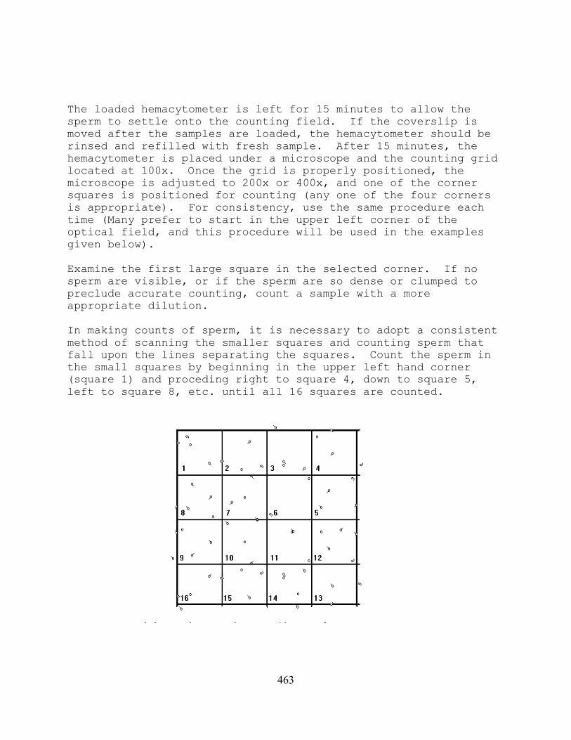
463

The loaded hemacytometer is left for 15 minutes to allow thesperm to settle onto the counting field. If the coverslip ismoved after the samples are loaded, the hemacytometer should berinsed and refilled with fresh sample. After 15 minutes, thehemacytometer is placed under a microscope and the counting gridlocated at 100x. Once the grid is properly positioned, themicroscope is adjusted to 200x or 400x, and one of the cornersquares is positioned for counting (any one of the four cornersis appropriate). For consistency, use the same procedure eachtime (Many prefer to start in the upper left corner of theoptical field, and this procedure will be used in the examplesgiven below).

Examine the first large square in the selected corner. If nosperm are visible, or if the sperm are so dense or clumped topreclude accurate counting, count a sample with a moreappropriate dilution.

In making counts of sperm, it is necessary to adopt a consistentmethod of scanning the smaller squares and counting sperm thatfall upon the lines separating the squares. Count the sperm inthe small squares by beginning in the upper left hand corner(square 1) and proceding right to square 4, down to square 5,left to square 8, etc. until all 16 squares are counted.

464

Because sperm that appear on lines might be counted as being ineither square, it is important to avoid double counting or non-counting. For this reason a convention is decided upon and usedconsistently: paraphrasing the instructions received with one(Hausser Scientific) counting chamber "to avoid counting (sperm)twice, the best practice is to count all touching the top andleft, and none touching the lower and right, boundary lines." Whatever convention is chosen, it must be adhered to. Theexample below shows a sperm count based upon a selectedconvention of counting sperm that fall on the upper and leftlines, but not on the lower or right lines:

In the above illustration, sperm falling on the lower and rightlines are not counted. The count begins at the upper left asillustrated in the preceding figure. A typical count sequence isdemonstrated by the numbers next to each sperm illustrated. Sperm identified as numbers 1, 5, 13, 20, 27, 28, 33, 51 and 54touch lines and are counted as being in the square below them orto their right. The circled sperm are not counted as being inthis field of 16 small squares (but they would be included in anycounts of adjacent squares in which they would be on upper orleft hand lines).

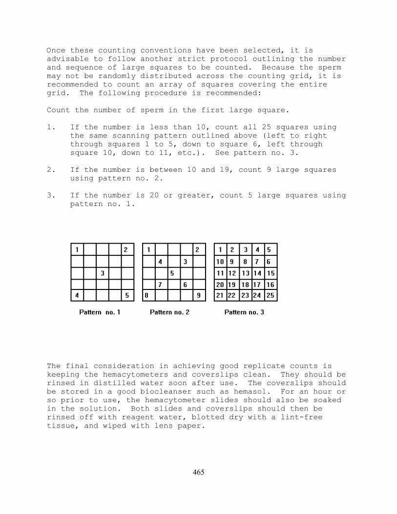
465

Once these counting conventions have been selected, it isadvisable to follow another strict protocol outlining the numberand sequence of large squares to be counted. Because the spermmay not be randomly distributed across the counting grid, it isrecommended to count an array of squares covering the entiregrid. The following procedure is recommended:

Count the number of sperm in the first large square.

1. If the number is less than 10, count all 25 squares usingthe same scanning pattern outlined above (left to rightthrough squares 1 to 5, down to square 6, left throughsquare 10, down to 11, etc.). See pattern no. 3.

2. If the number is between 10 and 19, count 9 large squaresusing pattern no. 2.

3. If the number is 20 or greater, count 5 large squares usingpattern no. 1.

The final consideration in achieving good replicate counts iskeeping the hemacytometers and coverslips clean. They should berinsed in distilled water soon after use. The coverslips shouldbe stored in a good biocleanser such as hemasol. For an hour orso prior to use, the hemacytometer slides should also be soakedin the solution. Both slides and coverslips should then berinsed off with reagent water, blotted dry with a lint-freetissue, and wiped with lens paper.

466

SECTION 17

GIANT KELP, Macrocystis pyriferaGERMINATION AND GERM-TUBE GROWTH TEST METHOD

Adapted from a method developed byBrian S. Anderson and John W. Hunt

Institute of Marine Sciences, University of CaliforniaSanta Cruz, California

(in association with)California Department of Fish and GameMarine Pollution Studies Laboratory

34500 Coast Route 1, Monterey, CA 93940

TABLE OF CONTENTS

17.1 Scope and Application17.2 Summary of Method17.3 Interferences17.4 Safety17.5 Apparatus and Equipment17.6 Reagents and Supplies17.7 Effluents and Receiving Water Collection,

Preservation, and Storage 17.8 Calibration and Standardization17.9 Quality Control 17.10 Test Procedures17.11 Summary of Test Conditions and Test

Acceptability Criteria17.12 Acceptability of Test Results17.13 Data Analysis17.14 Precision and Accuracy

Appendix I Step-by Step Summary

467

SECTION 17

GIANT KELP, MACROCYSTIS PYRIFERA GERMINATION AND GROWTH TEST

17.1 SCOPE AND APPLICATION

17.1.1 This method estimates the chronic toxicity of effluentsand receiving water to zoospores and embryonic gametophytes ofgiant kelp, Macrocystis pyrifera during a 48-h static non-renewalexposure. The effects include the synergistic, antagonistic, andadditive effects of all the chemical, physical, and biologicalcomponents which adversely affect the physiological andbiochemical functions of the test organisms.

17.1.2 Detection limits of the toxicity of an effluent orchemical substance are organism dependent.

17.1.3 Brief excursions in toxicity may not be detected using24-h composite samples. Also, because of the long samplecollection period involved in composite sampling and because thetest chambers are not sealed, highly volatile and highlydegradable toxicants in the source may not be detected in thetest.

17.1.4 This method is commonly used in one of two forms: (1) adefinitive test, consisting of minimum of five effluentconcentrations and a control, and (2) a receiving water test(s),consisting of one or more receiving water concentrations and acontrol.

17.1.5 This method should be restricted to use by, or under thesupervision of, professionals experienced in aquatic toxicitytesting. Specific experience with any toxicity test is usuallyneeded before acceptable results become routine.

17.2 SUMMARY OF METHOD

17.2.1 This method provides step-by-step instructions forperforming a 48-h day static non-renewal toxicity test usinggiant kelp to determine the toxicity of substances in marine and

468

estuarine waters. The test endpoints are germination ofgameophyte spores and length of embryonic gametophyte germinationtubes.

17.3 INTERFERENCES

17.3.1 Toxic substances may be introduced by contaminants indilution water, glassware, sample hardware, and testing equipment(see Section 5, Facilities and Equipment, and Supplies).

17.3.2 Improper effluent sampling and handling may adverselyaffect test results (see Section 8, Effluent and Receiving WaterSampling, and Sample Handling, and Sample Preparation forToxicity Tests).

17.4 SAFETY

17.4.1 See Section 3, Health and Safety.

17.5 APPARATUS AND EQUIPMENT

17.5.1 Tanks, trays, or aquaria -- for holding and acclimatinggiant kelp, e.g., standard salt water aquarium or Instant OceanAquarium (capable of maintaining seawater at 10-20EC), withappropriate filtration and aeration system.

17.5.2 Air pump, air lines, and air stones -- for aerating watercontaining broodstock or for supplying air to test solutions withlow dissolved oxygen.

17.5.3 Constant temperature chambers or water baths -- formaintaining test solution temperature and keeping dilution watersupply, gametes, and embryo stock suspensions at test temperature(15EC) prior to the test.

17.5.4 Water purification system -- Millipore Super-Q, Deionizedwater (DI) or equivalent.

17.5.5 Refractometer -- for determining salinity.

17.5.6 Hydrometer(s) -- for calibrating refractometer.

469

17.5.7 Thermometers, glass or electronic, laboratory grade --for measuring water temperatures.

17.5.8 Thermometer, National Bureau of Standards Certified (seeUSEPA METHOD l70.l, USEPA, l979) -- to calibrate laboratorythermometers.

17.5.9 pH and DO meters -- for routine physical and chemicalmeasurements.

17.5.10 Standard or micro-Winkler apparatus -- for determiningDO (optional) and calibrating the DO meter.

17.5.11 Winkler bottles -- for dissolved oxygen determinations.

17.5.12 Balance -- Analytical, capable of accurately weighing to0.0001 g.

17.5.13 Fume hood -- to protect the analyst from effluent orformaldehyde fumes.

17.5.14 Glass stirring rods -- for mixing test solutions.

17.5.15 Graduated cylinders -- Class A, borosilicate glass ornon-toxic plastic labware, 50-l000 mL for making test solutions. (Note: not to be used interchangeably for gametes or embryos andtest solutions).

17.5.16 Volumetric flasks -- Class A, borosilicate glass or non-toxic plastic labware, 10-1000 mL for making test solutions.

17.5.17 Pipets, automatic -- adjustable, to cover a range ofdelivery volumes from 0.010 to 1.000 mL.

17.5.18 Pipet bulbs and fillers -- PROPIPET® or equivalent.

17.5.19 Wash bottles -- for reagent water, for topping offgraduated cylinders, for rinsing small glassware and instrumentelectrodes and probes.

17.5.20 Wash bottles -- for dilution water.

470

17.5.21 20-liter cubitainers or polycarbonate water cooler jugs-- for making hypersaline brine.

17.5.22 Cubitainers, beakers, or similar chambers of non-toxiccomposition for holding, mixing, and dispensing dilution waterand other general non-effluent, non-toxicant contact uses. Theseshould be clearly labeled and not used for other purposes.

17.5.23 Beakers, 250 borosilicate glass -- for mixing testsolutions.

17.5.24 Beakers, 1,000 mL borosilicate glass -- for holdingsporophyll blades.

17.5.25 Inverted or compound microscope -- for inspectingzoopspores and embryonic gametophytes.

17.5.26 Hemacytometer (bright-line rbc) -- for measuringzoospore density.

17.5.27 Counter, two unit, 0-999 -- for recording counts ofzoopspores.

17.5.28 Light meter (irradiance meter w/cosine corrected sensor)-- for measuring light intensity.

17.5.29 Cool white fluorescent lights -- for providing lightduring incubation of developing gametophytes.

17.5.30 60 µm NITEX® filter -- for filtering receiving water.

17.6 REAGENTS AND SUPPLIES

17.6.1 Sample containers -- for sample shipment and storage (seeSection 8, Effluent and Receiving Water Sampling, and SampleHandling, and Sample Preparation for Toxicity Tests).

17.6.2 Data sheets (one set per test) -- for data recording(Figures 1 and 2).

17.6.3 Tape, colored -- for labelling test chambers andcontainers.

471

17.6.4 Markers, water-proof -- for marking containers, etc.

17.6.5 Parafilm -- to cover graduated cylinders and vessels.

17.6.6 Gloves, disposable -- for personal protection fromcontamination.

17.6.7 Pipets, serological -- l-l0 mL, graduated.

17.6.8 Pipet tips -- for automatic pipets.

17.6.9 Coverslips -- for microscope slides.

17.6.10 Lens paper -- for cleaning microscope optics.

17.6.11 Laboratory tissue wipes -- for cleaning and dryingelectrodes, microscope slides, etc.

17.6.12 Disposable countertop covering -- for protection of worksurfaces and minimizing spills and contamination.

17.6.13 pH buffers 4, 7, and l0 (or as per instructions ofinstrument manufacturer) -- for standards and calibration check(see USEPA Method l50.l, USEPA, l979).

17.6.14 Membranes and filling solutions -- for dissolved oxygenprobe (see USEPA Method 360.l, USEPA, l979), or reagents formodified Winkler analysis.

17.6.15 Laboratory quality assurance samples and standards --for the above methods.

17.6.16 Test chambers -- 600 mL, five chambers perconcentration. The chambers should be borosilicate glass (foreffluents) or nontoxic disposable plastic labware (for referencetoxicants). To avoid contamination from the air and excessiveevaporation of test solutions during the test, the chambersshould be covered during the test with safety glass plates or aplastic sheet (6 mm thick).

17.6.17 Glutaraldehyde -- for specimen preservation - optional;(see Section 17.10.8.2).

472

17.6.18 Microscope slide (flat) -- for each test chamber toserve as the substratum upon which the zoospores will settle.

17.6.19 Reference toxicant solutions (see Section 17.10.2.4 andsee Section 4, Quality Assurance).

17.6.20 Reagent water -- defined as distilled or deionized waterthat does not contain substances which are toxic to the testorganisms (see Section 5, Facilities, Equipment, and Supplies andSection 7, Dilution Water).

17.6.21 Effluent and receiving water -- see Section 8, Effluentand Surface Water Sampling, and Sample Handling, and SamplePreparation for Toxicity Tests.

17.6.22 Dilution water and hypersaline brine -- see Section 7,Dilution Water and Section 17.6.24, Hypersaline Brines. Thedilution water should be uncontaminated 1-µm-filtered naturalseawater. Hypersaline brine should be prepared from dilutionwater.

17.6.23 HYPERSALINE BRINES

17.6.23.1 Most industrial and sewage treatment effluentsentering marine and estuarine systems have little measurablesalinity. Exposure of larvae to these effluents will usuallyrequire increasing the salinity of the test solutions. It isimportant to maintain an essentially constant salinity across alltreatments. In some applications it may be desirable to matchthe test salinity with that of the receiving water (See Section7.1). Two salt sources are available to adjust salinities --artificial sea salts and hypersaline brine (HSB) derived fromnatural seawater. Use of artificial sea salts is necessary onlywhen high effluent concentrations preclude salinity adjustment byHSB alone.

17.6.23.2 Hypersaline brine (HSB) can be made by concentratingnatural seawater by freezing or evaporation. HSB should be madefrom high quality, filtered seawater, and can be added to theeffluent or to reagent water to increase salinity. HSB hasseveral desirable characteristics for use in effluent toxicitytesting. Brine derived from natural seawater contains thenecessary trace metals, biogenic colloids, and some of the

473

microbial components necessary for adequate growth, survival,and/or reproduction of marine and estuarine organisms, and it canbe stored for prolonged periods without any apparent degradation. However, even if the maximum salinity HSB (100‰) is used as adiluent, the maximum concentration of effluent (0‰) that can betested is 66% effluent at 34‰ salinity (see Table 1).

TABLE 1. MAXIMUM EFFLUENT CONCENTRATION (%) THAT CAN BE TESTED AT 34‰ WITHOUT THE ADDITION OF DRY SALTS GIVEN THE INDICATED EFFLUENT AND BRINE SALINITIES.

Effluent Brine Brine Brine Brine Brine

Salinity‰

60‰

70‰

80‰

90‰

100‰

0 43.33 51.43 57.50 62.22 66.00

1 44.07 52.17 58.23 62.92 66.67

2 44.83 52.94 58.97 63.64 67.35

3 45.61 53.73 59.74 64.37 68.04

4 46.43 54.55 60.53 65.12 68.75

5 47.27 55.38 61.33 65.88 69.47

10 52.00 60.00 65.71 70.00 73.33

15 57.78 65.45 70.77 74.67 77.65

20 65.00 72.00 76.67 80.00 82.50

25 74.29 80.00 83.64 86.15 88.00

17.6.23.3 High quality (and preferably high salinity) seawatershould be filtered to at least 10 µm before placing into thefreezer or the brine generator. Water should be collected on anincoming tide to minimize the possibility of contamination.

17.6.23.4 Freeze Preparation of Brine

17.6.23.4.1 A convenient container for making HSB by freezing isone that has a bottom drain. One liter of brine can be made from

474

four liters of seawater. Brine may be collected by partiallyfreezing seawater at -10 to -20EC until the remaining liquid hasreached the target salinity. Freeze for approximately six hours,then separate the ice (composed mainly of fresh water) from theremaining liquid (which has now become hypersaline).

17.6.23.4.2 It is preferable to monitor the water until thetarget salinity is achieved rather than allowing total freezingfollowed by partial thawing. Brine salinity should never exceed100‰. It is advisable not to exceed about 70‰ brine salinityunless it is necessary to test effluent concentrations greaterthan 50%.

17.6.23.4.3 After the required salinity is attained, the HSBshould be filtered through a 1 µm filter and poured directly intoportable containers (20-L cubitainers or polycarbonate watercooler jugs are suitable). The brine storage containers shouldbe capped and labelled with the salinity and the date the brinewas generated. Containers of HSB should be stored in the dark at4EC (even room temperature has been acceptable). HSB is usuallyof acceptable quality even after several months in storage.

17.6.23.5 Heat Preparation of Brine

17.6.23.5.1 The ideal container for making brine using heat-assisted evaporation of natural seawater is one that (1) has ahigh surface to volume ratio, (2) is made of a non-corrosivematerial, and (3) is easily cleaned (fiberglass containers areideal). Special care should be used to prevent any toxicmaterials from coming in contact with the seawater being used togenerate the brine. If a heater is immersed directly into theseawater, ensure that the heater materials do not corrode or leach any substances that would contaminate the brine. Onesuccessful method is to use a thermostatically controlled heatexchanger made from fiberglass. If aeration is needed, use onlyoil-free air compressors to prevent contamination. 17.6.23.5.2 Before adding seawater to the brine generator,thoroughly clean the generator, aeration supply tube, heater, andany other materials that will be in direct contact with thebrine. A good quality biodegradable detergent should be used,followed by several (at least three) thorough reagent waterrinses.

475

17.6.23.5.3 Seawater should be filtered to at least 10 µm beforebeing put into the brine generator. The temperature of theseawater is increased slowly to 40EC. The water should beaerated to prevent temperature stratification and to increasewater evaporation. The brine should be checked daily (dependingon the volume being generated) to ensure that the salinity doesnot exceed 100‰ and that the temperature does not exceed 40EC. Additional seawater may be added to the brine to obtain thevolume of brine required.

17.6.23.5.4 After the required salinity is attained, the HSBshould be filtered through a 1 µm filter and poured directly intoportable containers (20-L cubitainers or polycarbonate watercooler jugs are suitable). The brine storage containers shouldbe capped and labelled with the salinity and the date the brinewas generated. Containers of HSB should be stored in the dark at4EC (even room temperature has been acceptable). HSB is usuallyof acceptable quality even after several months in storage.

17.6.23.6 Artificial Sea Salts

17.6.23.6.1 No data from giant kelp tests using sea salts orartificial seawater (e.g., GP2) are available for evaluation atthis time, and their use must be considered provisional.

17.6.23.7 Dilution Water Preparation from Brine

17.6.23.7.1 Although salinity adjustment with brine is thepreferred method, the use of high salinity brines and/or reagentwater has sometimes been associated with discernible adverseeffects on test organisms. For this reason, it is recommendedthat only the minimum necessary volume of brine and reagent waterbe used to offset the low salinity of the effluent, and thatbrine controls be included in the test. The remaining dilutionwater should be natural seawater. Salinity may be adjusted inone of two ways. First, the salinity of the highest effluenttest concentration may be adjusted to an acceptable salinity, andthen serially diluted. Alternatively, each effluentconcentration can be prepared individually with appropriatevolumes of effluent and brine.

17.6.23.7.2 When HSB and reagent water are used, thoroughlymix together the reagent water and HSB before mixing in the

476

effluent. Divide the salinity of the HSB by the expected testsalinity to determine the proportion of reagent water to brine. For example, if the salinity of the brine is 100‰ and the test isto be conducted at 34‰, 100‰ divided by 34‰ = 2.94. Theproportion of brine is 1 part, plus 1.94 parts reagent water. Tomake 1 L of dilution water at 34‰ salinity from a HSB of 100‰,340 mL of brine and 660 mL of reagent water are required. Verifythe salinity of the resulting mixture using a refractometer.

17.6.23.8 Test Solution Salinity Adjustment

17.6.23.8.1 Table 2 illustrates the preparation of testsolutions (up to 50% effluent) at 34‰ by combining effluent, HSB,and dilution water. Note: if the highest effluent concentrationdoes not exceed 50% effluent, it is convenient to prepare brineso that the sum of the effluent salinity and brine salinityequals 68‰; the required brine volume is then always equal to theeffluent volume needed for each effluent concentration as in theexample in Table 2. 17.6.23.8.2 Check the pH of all test solutions and adjust towithin 0.2 units of dilution water pH by adding, dropwise, dilutehydrochloric acid or sodium hydroxide (see Section 8.8.9,Effluent and Receiving Water Sampling, Sample Handling, andSample Preparation for Toxicity Tests).

17.6.23.8.3 To calculate the amount of brine to add to eacheffluent dilution, determine the following quantities: salinityof the brine (SB, in ‰), the salinity of the effluent (SE, in ‰), and volume of the effluent to be added (VE, in mL). Then usethe following formula to calculate the volume of brine (VB, inmL) to be added:

VB = VE x (34 - SE)/(SB - 34)

17.6.23.8.4 This calculation assumes that dilution watersalinity is 34 ± 2‰.

17.6.23.9 Preparing Test Solutions

17.6.23.9.1 Two hundred mL of test solution are needed for eachtest chamber. To prepare test solutions at low effluentconcentrations (<6%), effluents may be added directly to dilution

477

water. For example, to prepare 1% effluent, add 10 mL ofeffluent to a 1-liter volumetric flask using a volumetric pipetor calibrated automatic pipet. Fill the volumetric flask to the1-Liter mark with dilution water, stopper it, and shake to mix. Distribute equal volumes into the replicate test chambers.

17.6.23.9.2 To prepare a test solution at higher effluentconcentrations, hypersaline brine must usually be used. Forexample, to prepare 40% effluent, add 400 mL of effluent to a 1-liter volumetric flask. Then, assuming an effluent salinity of2‰ and a brine salinity of 66‰, add 400 mL of brine (see equationabove and Table 2) and top off the flask with dilution water. Stopper the flask and shake well. Distribute equal volumes intothe replicate test chambers.

17.6.23.10 Brine Controls

17.6.23.10.1 Use brine controls in all tests where brine isused. Brine controls contain the same volume of brine as doesthe highest effluent concentration using brine, plus the volumeof reagent water needed to reproduce the hyposalinity of theeffluent in the highest concentration, plus dilution water. Calculate the amount of reagent water to add to brine controls byrearranging the above equation, (See, 17.6.23.8.3) setting SE =0, and solving for VE.

VE = VB x (SB - 34)/(34 - SE)

If effluent salinity is essentially 0‰, the reagent water volumeneeded in the brine control will equal the effluent volume at thehighest test concentration. However, as effluent salinity andeffluent concentration increase, less reagent water volume isneeded.

17.6.24 TEST ORGANISMS

17.6.24.1 The test organisms for this method are the zoosporesof the giant kelp, Macrocystis pyrifera. Macrocystis is thedominant canopy forming Laminarian alga in southern and centralCalifornia and forms extensive subtidal forests along the coast.Giant kelp forests support a rich diversity of marine life andprovide habitat and food for hundreds of invertebrate andvertebrate species (North, 1971; Foster and Schiel, 1985). It

478

TABLE 2. EXAMPLES OF EFFLUENT DILUTION SHOWING VOLUMES OFEFFLUENT (x‰), BRINE, AND DILUTION WATER NEEDED FOR ONELITER OF EACH TEST SOLUTION.

FIRST STEP: Combine brine with reagent water or natural seawaterto achieve a brine of 68-x‰ and, unless natural seawater is usedfor dilution water, also a brine-based dilution water of 34‰.

SERIAL DILUTION:Step 1. Prepare the highest effluent concentration to be testedby adding equal volumes of effluent and brine to the appropriatevolume of dilution water. An example using 40% is shown.

Effluent Conc.(%)

Effluent x‰ Brine (68-x)‰

Dilution Water*34‰

40 800 mL 800 mL 400 mL

Step 2. Use either serially prepared dilutions of the highest testconcentration or individual dilutions of 100% effluent.

Effluent Conc. (%) Effluent Source Dilution Water* (34‰)

20 1000 mL of 40% 1000 mL

10 1000 mL of 20% 1000 mL

5 1000 mL of 10% 1000 mL

2.5 1000 mL of 5% 1000 mL

Control none 1000 mL

INDIVIDUAL PREPARATION

Effluent Conc.(%)

Effluent x‰ Brine (68-x)‰ Dilution Water*34‰

40 400 mL 400 mL 200 mL

20 200 mL 200 mL 600 mL

10 100 mL 100 mL 800 mL

5 50 mL 50 mL 900 mL

2.5 25 mL 25 mL 950 mL

Control none none 1000 mL

*May be natural seawater or brine-reagent water equivalent.

479

is an appropriate toxicity test species because of itsavailability, economic and ecological importance, history ofsuccessful laboratory culture (North, 1976; Luning, 1980;Kuwabara, 1981; Deysher and Dean, 1984; Linfield, 1985), andprevious use in toxicity testing (Smith and Harrison, 1978; Jameset al., 1987; Anderson and Hunt, 1988; Hunt et al., 1989;Anderson et al., 1990). Other Laminarian alga species haveproven to be useful for laboratory toxicity testing (Chung andBrinkhuis, 1986; Thompson and Burrows, 1984; Hopkin and Kain,1978; see Thursby et al., 1993 for review).

17.6.24.2 Like all kelps, Macrocystis has a life cycle thatalternates between a microscopic gametophyte stage and amacroscopic sporophyte stage. It is the sporophyte stage thatforms kelp forests. These plants produce reproductive blades(sporophylls) at their base. The sporophylls develop patches(sori) in which biflagellate, haploid zoospores are produced. The zoospores are released into the water column where they swimand eventually settle onto the bottom and germinate. Thedioecious spores develop into either male or female gametophytes. The male gametophytes produce flagellated gametes which mayfertilize eggs produced by the female gametophytes. Fertilizedeggs develop into sporophytes within 12- 15 days, completing thelifecycle.

17.6.24.3 The method described here focuses on germination ofthe zoospores and the initial growth of the developinggametophytes. It involves the controlled release of zoosporesfrom the sporophyll blades, followed by the introduction of aspore suspension of known density into the test containers. Thezoospores swim through the test solution and eventually settleonto glass microscope slides. The settled spores germinate byextruding the cytoplasm of the spore through the germ-tube intothe first gametophytic cell. This stage is often referred to asthe "dumbell" stage. The two endpoints measured after 48 hoursare germination success and growth of the embryonic gametophytes(germ-tube length).

17.6.24.4 Species Identification

17.6.24.4.1 Although there is some debate over the taxonomy ofthe genus Macrocystis, Abbott and Hollenberg (1976) consider onlytwo species in California: M. pyrifera, and M. integrifolia. The

480

two are distinguished from each other based on habitat and themorphology of their holdfasts. Macrocystis pyrifera occurssubtidally while M. integrifolia occurs in the low intertidaland shallow subtidal zones. Macrocystis pyrifera has a conicalholdfast while M. integrifolia has a more flattened, creepingholdfast. Consult Abbott and Hollenberg (1976) for a moredetailed taxonomic discussion of the two species.

17.6.24.5 Obtaining Zoospores

17.6.24.5.1 Macrocystis zoospores are obtained from thereproductive blades (sporophylls) of the adult plant. The sporophylls are located near the base of the plant just above itsconical holdfast. Sporophylls must be collected subtidally andshould be collected from at least five different plants in anyone location to give a good genetic representation of thepopulation. The sporophylls should be collected from areas freeof point and non-point source pollution to minimize thepossibility of genetic or physiological adaptation to pollutants. In situations where a thermocline is present at the collectionsite, the sporophylls should be collected from below thethermocline to ensure adequate spore release. Sporophylls areidentified in the field by the presence of darkened patchescalled sori. The zoospores develop within the sori. In addition,the sporophylls are distinguished from vegetative blades by theirthinner width, basal location on the adult plant, and generallack of pneumatocysts (air bladders). Collection of algae isregulated by California law. Collectors must obtain a scientificcollector's permit from the California Department of Fish andGame and observe any regulations regarding collection andtransport of kelp. For further information regarding sporophyllcollection, contact the Marine Pollution Studies Laboratory,34500 Coast Route 1, Granite Canyon, Monterey CA, 93940, (408)624-0947.

17.6.24.6 Broodstock Culture and Handling

17.6.24.6.1 After collection, the sporophylls should be keptdamp and not exposed to direct sunlight. Avoid immersing theblades in seawater, however, to prevent premature spore release.The sporophylls should be rinsed thoroughly in 0.2 µm filteredseawater to remove diatoms and other epiphytic organisms. Theindividual blades can be gently rubbed between fingers under

481

running filtered seawater or brushed with a soft bristled brush.The blades are stored between moist paper towels (lasagna styleso that the sporophylls do not overlap each other, and each layerof sporophylls are separated by a layer of paper towels) atapproximately 9-12EC until needed. The zoospores must bereleased within 24 hours of collection to insure their viability. Preliminary data indicate that prolonged storage times may affecttest results (Bottomley et al., 1991); however as long asgermination rates meet control acceptability criteria this shouldnot affect test results. Sporophylls should be kept shaded toprevent damage to the spores. For holding or transport timeslonger than approximately six hours, the sporophylls should beplaced in an ice chest with blue ice. The blue ice should bewrapped in newspaper (10 layers) for insulation, then plastic toprevent leaking.

17.7 EFFLUENT AND RECEIVING WATER COLLECTION, PRESERVATION, AND STORAGE

17.7.1 See Section 8, Effluent and Receiving Water Sampling,Sample Handling, and Sample Preparation for Toxicity Tests.

17.8 CALIBRATION AND STANDARDIZATION

17.8.1 See Section 4, Quality Assurance.

17.9 QUALITY CONTROL

17.9.1 See Section 4, Quality Assurance.

17.10 TEST PROCEDURES

17.10.1 TEST DESIGN

17.10.1.1 The test consists of at least five effluentconcentrations plus a dilution water control. Tests that usebrine to adjust salinity must also contain five replicates of abrine control.

17.10.1.2 Effluent concentrations are expressed as percenteffluent.

17.10.2 TEST SOLUTIONS

482

17.10.2.1 Receiving waters

17.10.2.1.1 The sampling point is determined by the objectivesof the test. At estuarine and marine sites, samples are usuallycollected at mid-depth. Receiving water toxicity is determinedwith samples used directly as collected or with samples passedthrough a 60 µm NITEX® filter and compared without dilution, against a control. Using five replicate chambers per test, eachcontaining 200 mL, analysis would require approximately 1 L ofsample per test.

17.10.2.2 Effluents

17.10.2.2.1 The selection of the effluent test concentrationsshould be based on the objectives of the study. A dilutionfactor of at least 0.5 is commonly used. A dilution factor of0.5 provides hypothesis test discrimination of ± 100%, andtesting of a 16 fold range of concentrations. Hypothesis testdiscrimination shows little improvement as dilution factors areincreased beyond 0.5 and declines rapidly if smaller dilutionfactors are used. USEPA recommends that one of the five effluenttreatments must be a concentration of effluent mixed withdilution water which corresponds to the permittee's instreamwaste concentration (IWC). At least two of the effluenttreatments must be of lesser effluent concentration than the IWC,with one being at least one-half the concentration of the IWC. If 100‰ HSB is used as a diluent, the maximum concentration ofeffluent that can be tested will be 66% at 34‰ salinity.

17.10.2.2.2 If the effluent is known or suspected to be highlytoxic, a lower range of effluent concentrations should be used(such as 25%, 12.5%, 6.25%, 3.12% and 1.56%).

17.10.2.2.3 The volume in each test chamber is 200 mL.

17.10.2.2.4 Effluent dilutions should be prepared for allreplicates in each treatment in one container to minimizevariability among the replicates. Dispense into the appropriateeffluent test chambers.

17.10.2.3 Dilution Water

17.10.2.3.1 Dilution water should be uncontaminated 1-µm-

483

filtered natural seawater or hypersaline brine prepared fromuncontaminated natural seawater plus reagent water (see Section7, Dilution Water). Natural seawater may be uncontaminatedreceiving water. This water is used in all dilution steps and asthe control water.

17.10.2.4 Reference Toxicant Test

17.10.2.4.1 Reference toxicant tests should be conducted asdescribed in Quality Assurance (see Section 4.7).

17.10.2.4.2 The preferred reference toxicant for giant kelp iscopper chloride (CuCl2N2H2O). Reference toxicant tests providean indication of the sensitivity of the test organisms and thesuitability of the testing laboratory (see Section 4 QualityAssurance). Another toxicant may be specified by the appropriateregulatory agency. Prepare a 10,000 µg/L copper stock solutionby adding 0.0268 g of copper chloride (CuCl2N2H2O) to one literof reagent water in a polyethylene volumetric flask. Alternatively, certified standard solutions can be ordered fromcommercial companies.

17.10.2.4.3 Reference toxicant solutions should be fivereplicates each of 0 (control), 5.6, 10, 18, 32, 100, and 180µg/L total copper. Prepare one liter of each concentration byadding 0, 0.56, 1.0, 1.8, 3.2, 5.6, 10.0, and 18.0 mL of stocksolution, respectively, to one-liter volumetric flasks and fillwith dilution water. Start with control solutions and progressto the highest concentration to minimize contamination.

17.10.2.4.4 If the effluent and reference toxicant tests are tobe run concurrently, then the tests must use zoospores from thesame release. The tests must be handled in the same way and testsolutions delivered to the test chambers at the same time. Reference toxicant tests must be conducted at 34 ± 2‰.

17.10.3 RELEASE OF ZOOSPORES FOR THE TEST

17.10.3.1 Zoospores are released by slightly desiccating thesporophyll blades, and then placing them in filtered seawater. To desiccate the sporophylls, blot the blades with paper towelsand expose them to air for 1 hour.

484

17.10.3.2 The number of sporophyll blades needed depends upontheir maturity; usually 25-30 blades (~ 100 grams wet weight) aresufficient. After 1 hour the blades should be rinsed againthoroughly using 0.2 µm-filtered seawater, then placed in a oneL glass or plastic beaker filled with 0.2 µm filtered seawater at15-16EC. The release water should never exceed 18EC.

17.10.3.3 After one hour, a sufficient number of zoosporesshould be present to conduct the test. The presence of zoosporesis indicated by a slight cloudiness in the water. To verifywhether zoospores are present, periodically sample the solutionand observe the sample microscopically (100x).

17.10.3.4 To insure that the zoospores are viable and have notbegun to germinate before they are exposed to the toxicant, thezoospore release process should not be longer than two hours. Ifit takes longer than two hours to get an adequate density ofzoospores (~7,500 zoospores/mL of test solution), repeat therelease process with a new batch of sporophylls.

17.10.3.5 After the zoospores are released, remove thesporophylls and let the spore mixture settle for 30 minutes. After 30 minutes, decant 250 mLs from the top of the sporesolution into a separate clean glass beaker. Sample the sporesolution and determine the spore density using a bright-linehemacytometer (100x). Spores may be counted directly, or toobtain a more accurate count, fix a sample of spores by mixingnine milliliters of spore solution with 1-mL of 37% bufferedformalin (or acetic acid) in a test tube. Shake the sample wellbefore placing it on the hemacytometer.

17.10.3.6 After counting, the density is multiplied by 1.111 tocorrect for the dilution caused by adding 1 mL of formalin to thesample. Use at least five replicate counts. After the densityis determined, calculate the volume of zoospores necessary togive approximately 7,500 spores/mL of test solution. To prevent over-dilution of the test solution, this volume should not exceed1% of the test solution volume. If this volume exceeds 1% of thetest solution volume, it should be noted in the results.

17.10.3.7 Test solutions must be prepared while the zoosporesare releasing from the sporophylls. Test solutions must bemixed, sampled, and temperature equilibrated in time to receive

485

the swimming zoospores as soon as they are counted. Zoosporerelease and counting should be done in a room separate from thatused for toxicant preparation, and care should be taken to avoidcontaminating the zoospores prior to testing.

17.10.4 START OF THE TEST

17.10.4.1 Prior to Beginning the Test

17.10.4.1.1 The test should begin as soon as possible,preferably within 24 h of sample collection. The maximum holdingtime following retrieval of the sample from the sampling deviceshould not exceed 36 h for off-site toxicity tests unlesspermission is granted by the permitting authority. In no caseshould the sample be used in a test more than 72 h after samplecollection (see Section 8 Effluent and Receiving Water Sampling,Sample Handling, and Sample Preparation for Toxicity Test).

17.10.4.1.2 Just prior to test initiation (approximately 1 h),the temperature of a sufficient quantity of the sample to makethe test solutions should be adjusted to the test temperature (15± 1EC) and maintained at that temperature during the addition ofdilution water.

17.10.4.1.3 Increase the temperature of the water bath, room, orincubator to the required test temperature (15 ± 1EC).

17.10.4.1.4 Randomize the placement of test chambers in thetemperature-controlled water bath, room, or incubator at thebeginning of the test, using a position chart. Assign numbersfor the position of each test chamber using a random numbers orsimilar process (see Appendix A, for an example ofrandomization). Maintain the chambers in this configurationthroughout the test, using a position chart. Record thesenumbers on a separate data sheet together with the concentrationand replicate numbers to which they correspond. Identify thissheet with the date, test organism, test number, laboratory, andinvestigator's name, and safely store it away until after thegametophyte spores have been examined at the end of the test.

17.10.4.1.5 Note: Loss of the randomization sheet wouldinvalidate the test by making it impossible to analyze the dataafterwards. Make a copy of the randomization sheet and store

486

separately. Take care to follow the numbering system exactlywhile filling chambers with the test solutions.

17.10.4.1.6 Arrange the test chambers randomly in the water bathor controlled temperature room. Once chambers have been labeledrandomly and filled with test solutions, they can be arranged in

numerical order for convenience, since this will also ensurerandom placement of treatments.

17.10.4.2 Estimation of Zoospore Density

17.10.4.2.1 After determining the zoospore density andcalculating the volume yielding 7,500 zoospores/mL test solution,add this volume to each test chamber (this is the start time ofthe test). Observe a sample of zoospores microscopically toverify that they are swimming before adding them to the testchambers.

17.10.4.2.2 Incubate the developing gametophytes for 48 hours inthe test chambers at 15EC under 50 µE/m2/s. The zoosporesgerminate and develop to the "dumbell" gametophyte stage duringthe exposure period.

17.10.5 LIGHT, PHOTOPERIOD, SALINITY AND TEMPERATURE

17.10.5.1 The lights used in this method are cool whitefluorescent lights adjusted to give 50 µE/m2/s at the top of eachtest chamber. Each test chamber must receive the same quanta oflight (50 ± 10 µE/m2/s). Areas of increased light can beeliminated by taping the outside of the light diffuser orwrapping the fluorescent bulbs with aluminum foil.

17.10.5.2 The water temperature in the test chambers should bemaintained at 15 ± 1EC. If a water bath is used to maintain thetest temperature, the water depth surrounding the test cupsshould be as deep as possible without floating the chambers.

15.10.5.3 The test salinity should be in the range of 34 ± 2‰. The salinity should vary by no more than ±2‰ among the chamberson a given day. If effluent and receiving water tests areconducted concurrently, the salinities of these tests should besimilar.

487

15.10.5.4 Rooms or incubators with high volume ventilationshould be used with caution because the volatilization of thetest solutions and evaporation of dilution water may cause wide fluctuations in salinity. Covering the test chambers with cleanpolyethylene plastic may help prevent volatilization andevaporation of the test solutions.

17.10.6 DISSOLVED OXYGEN (DO) CONCENTRATION

17.10.6.1 Aeration may affect the toxicity of effluent andshould be used only as a last resort to maintain a satisfactoryDO. The DO concentration should be measured on new solutions atthe start of the test (Day 0). The DO should not fall below 4.0mg/L (see Section 8, Effluent and Receiving Water Sampling,Sample Handling, and Sample Preparation for Toxicity Tests). Ifit is necessary to aerate, all treatments and the control shouldbe aerated. The aeration rate should not exceed that necessaryto maintain a minimum acceptable DO and under no circumstancesshould it exceed 100 bubbles/minute, using a pipet with a 1-2 mmorifice, such as a 1 mL KIMAX® serological pipet No. 37033, orequivalent.

17.10.7 OBSERVATIONS DURING THE TEST

17.10.7.1 Routine Chemical and Physical Observations

17.10.7.1.1 DO is measured at the beginning of the exposureperiod in one test chamber at each test concentration and in thecontrol.

17.10.7.1.2 Temperature, pH, and salinity are measured at thebeginning of the exposure period in one test chamber at eachconcentration and in the control. Temperature should also bemonitored continuously or observed and recorded daily for atleast two locations in the environmental control system or thesamples. Temperature should be measured in a sufficient numberof test chambers at the end of the test to determine temperaturevariation in the environmental chamber.

17.10.7.1.3 Record all the measurements on the data sheet.

17.10.8 TERMINATION OF THE TEST

488

17.10.8.1 Ending the Test

17.10.8.1.1 Record the time the test is terminated.

17.10.8.1.2 Temperature, pH, dissolved oxygen, and salinity aremeasured at the end of the exposure period in one test chamber ateach concentration and in the control.

17.10.8.2 Sample preservation

17.10.8.2.1 In some cases it may be convenient to preserve thekelp cultures for later analysis. Preliminary work by Andersonand Hunt (Marine Pollution Studies Laboratory unpublished data)indicates that cultures can be preserved in 0.1% glutaraldehyde(final concentration) and that preservation has no significanteffect on germination or germ-tube growth. Other researchershave used higher glutaraldehyde concentrations and found adequatepreservation with no effect on spore germination or gametophytegrowth (K. Goodwin, Calif. Inst. of Tech., unpublished data).

17.10.8.2.2 Because data on the effects of preservation arepreliminary, it is recommended that anyone interested inpreserving kelp cultures for later analysis first demonstratethat preservation does not affect test results. This can beaccomplished by comparing germination and germ-tube growth inpreserved vs non-preserved kelp cultures. We also recommend thatif it is necessary to preserve kelp cultures for later analysis,a complete test should be preserved so that if any replicates areread preserved, all of the replicates should be read preserved. In the case where concurrent reference toxicant and complexeffluent tests are conducted, it may be convenient to fix onetest in glutaraldehyde and read the other test immediately.

17.10.8.2.3 When fixing kelp cultures, it is important tominimize disturbance to the gametophytes. Make sure that theculture slides are fixed and stored horizontally. We have useddisposable petri dishes for preservation chambers; these allowindividual replicate slides to be labelled and preservedseparately to avoid mixing replicates. Note: Glutaraldehyde istoxic. If you intend to use this material as a preservative,study the material data safety sheets from the supplier and

489

follow strict safety precautions. Make sure test chambers andsolutions contaminated with this material are disposed ofproperly.

17.10.8.3 Counting

17.10.8.3.1 After 48 hours, the test is terminated. Because ittakes a considerable amount of time to read the test, reading canbegin after 45 hours and must be completed within six hours. Remove the slide without decanting the test solution. The testslide can be lifted from the bottom of the test chamber with aseparate clean microscope slide. Blot the bottom on a papertowel and place an 18-mm square cover slip on the slide. Blotthe excess water around the edge of the cover slip to eliminatethe flow of water under the cover slip.

17.10.8.4 Endpoints

17.10.8.4.1 The endpoints measured for the 48 hour Macrocystismethod are percent germination success and germination tubelength. Germination is considered successful if a germ-tube ispresent on the settled zoospore. Germination is considered to beunsuccessful if no germination tube is visible. To differentiatebetween a germinated and non-germinated zoospore, observe thesettled zoospores at 400x magnification and determine whetherthey are circular (non-germinated) or have a protuberance thatextends at least one spore diameter (about 3.0 µm) from the edgeof the spore (germinated). Spores with a germination tubes lessthan one spore diameter are considered non-germinated.

17.10.8.4.2 The first 100 spores encountered while moving acrossthe microscope slide are counted for each replicate of eachtreatment. Note: Sewage effluents may contain certain objects,such as ciliates, which look similar to non-germinated kelpspores. It is important to ensure that only kelp spores arecounted for this endpoint. Kelp spores are green-brown in color,spherical, and lack mobility. Also, components of the cytoplasmof kelp spores appear to fluoresce a light green color when thespore is slightly out of focus. If a particular object cannot beidentified, it should not be counted.

17.10.8.4.3 The growth endpoint is the measurement of the totallength of the germination tube from the edge of the original

490

spore membrane. Only germinated spores with straight germinationtubes and within the same focal plane are measured; if a spore isnot completely in focus from tip to tip it should not bemeasured. The spores to be measured are randomly selected bymoving the microscope stage to a new field of view withoutlooking through the ocular lens.

17.10.8.4.4 Measure the germination-tube length of the sporewhose spore case center is nearest the micrometer in each field;the spores case can be distinguished from the growing tip becauseit is usually clear (empty) at 48 hours, and it is more circularthan the growing tip. If more than one spore case is touchingthe micrometer, both (or all) germinated spores are measured. Atotal of 10 spores for each replicate of each treatment aremeasured. It is easier to measure germ-tube length with amicrometer having a 10 mm linear scale (0.1 mm subdivisions);measure lengths to the nearest micron (typically to the nearesthalf micrometer unit; see Section 10200E, Standard Methods 17thedition, for micrometer/microscope calibration procedures). Insituations where germination is significantly inhibited it may bedifficult to find germinated spores for germ-tube growthmeasurement using the random search technique.

17.10.8.4.5 To expedite reading, the slide can be scanned tofind germinated spores if germination is 30% or less. In thissituation the first 10 spores encountered are measured for germ-tube length.

17.11 SUMMARY OF TEST CONDITIONS AND TEST ACCEPTABILITY CRITERIA

17.11.1 A summary of test conditions and test acceptabilitycriteria is listed in Table 3.

17.12 ACCEPTABILITY OF TEST RESULTS

17.12.1 For tests to be considered acceptable, the followingrequirements must be met:

(1) Mean control germination must be at least 70% in thecontrols.

(2) Mean germination-tube length in the controls must be atleast 10 µm in the controls.

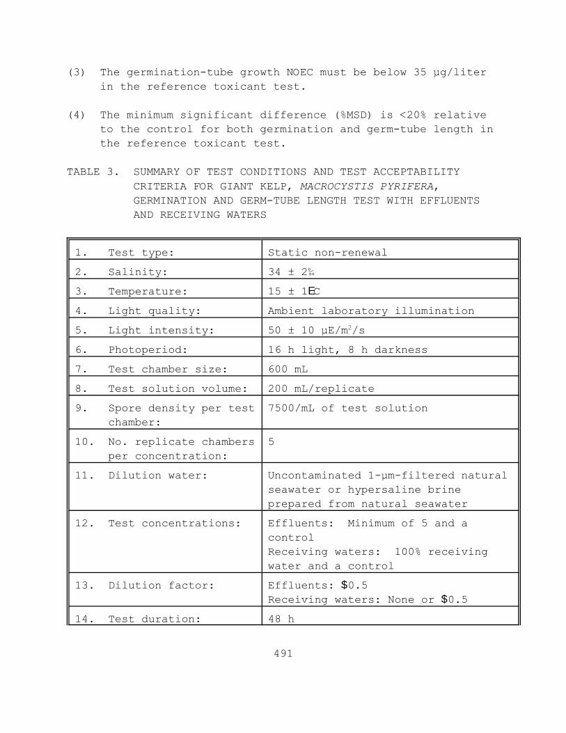
491

(3) The germination-tube growth NOEC must be below 35 µg/literin the reference toxicant test.

(4) The minimum significant difference (%MSD) is <20% relativeto the control for both germination and germ-tube length inthe reference toxicant test.

TABLE 3. SUMMARY OF TEST CONDITIONS AND TEST ACCEPTABILITYCRITERIA FOR GIANT KELP, MACROCYSTIS PYRIFERA,GERMINATION AND GERM-TUBE LENGTH TEST WITH EFFLUENTSAND RECEIVING WATERS

1. Test type: Static non-renewal

2. Salinity: 34 ± 2‰

3. Temperature: 15 ± 1EC

4. Light quality: Ambient laboratory illumination

5. Light intensity: 50 ± 10 µE/m2/s

6. Photoperiod: 16 h light, 8 h darkness

7. Test chamber size: 600 mL

8. Test solution volume: 200 mL/replicate

9. Spore density per testchamber:

7500/mL of test solution

10. No. replicate chambersper concentration:

5

11. Dilution water: Uncontaminated 1-µm-filtered naturalseawater or hypersaline brineprepared from natural seawater

12. Test concentrations: Effluents: Minimum of 5 and acontrolReceiving waters: 100% receivingwater and a control

13. Dilution factor: Effluents: $0.5Receiving waters: None or $0.5

14. Test duration: 48 h

492

15. Endpoints: Germination and germ-tube length

16. Test acceptabilitycriteria:

$70% germination in the controls;$10 µm germ-tube length in thecontrols and the NOEC must be below35 µg/L in the reference toxicanttest; must achieve a %MSD of <20 forboth germination and germ-tubelength in the reference toxicant.

17. Sampling requirements: One sample collected at testinitiation, and preferably usedwithin 24 h of the time it isremoved from the sampling device(see Section 8, Effluent andReceiving Water Sampling, SampleHandling, and Sample Preparation forToxicity Tests)

18. Sample volumerequired:

2 L per test

17.13 DATA ANALYSIS

17.13.1 GENERAL

17.13.1.1 Tabulate and summarize the data. Table 4 presents asample set of germination and growth data.

17.13.1.2 The endpoints of the giant kelp 48-hour chronic testare based on the adverse effects on germination and growth. TheIC25 endpoints are calculated using point estimation techniques(see Section 9, Chronic Toxicity Test Endpoints and DataAnalysis). LOEC and NOEC values for germination and growth areobtained using a hypothesis testing approach such as Dunnett'sProcedure (Dunnett, 1955) or Steel's Many-one Rank Test (Steel,1959; Miller, 1981) (see Section 9). Separate analyses areperformed for the estimation of the LOEC and NOEC endpoints andfor the estimation of the IC25 endpoints. Concentrations atwhich there is no germination in any of the test chambers areexcluded from the statistical analysis of the NOEC and LOEC forgermination and growth, but included in the estimation of the

493

IC25. See the Appendices for examples of the manualcomputations, and examples of data input and program output.

17.13.1.3 The statistical tests described here must be used witha knowledge of the assumptions upon which the tests arecontingent. The assistance of a statistician is recommended foranalysts who are not proficient in statistics.

17.13.2 EXAMPLE OF ANALYSIS OF GIANT KELP, MACROCYSTIS PYRIFERA,GERMINATION DATA

17.13.2.1 Formal statistical analysis of the germination data isoutlined in Figure 1. The response used in the analysis is theproportion of germinated spores in each test or control chamber. Separate analyses are performed for the estimation of the NOECand LOEC endpoints and for the estimation of the IC25 endpoint. Concentrations at which there is no germination in any of thetest chambers are excluded from statistical analysis of the NOECand LOEC, but included in the estimation of the IC endpoints.

17.13.2.2 For the case of equal numbers of replicates across allconcentrations and the control, the evaluation of the NOEC andLOEC endpoints is made via a parametric test, Dunnett'sProcedure, or a nonparametric test, Steel's Many-one Rank Test,on the arc sine square root transformed data. Underlyingassumptions of Dunnett's Procedure, normality and homogeneity ofvariance, are formally tested. The test for normality is theShapiro-Wilk's Test, and Bartlett's Test is used to test forhomogeneity of variance. If either of these tests fails, thenonparametric test, Steel's Many-one Rank Test, is used todetermine the NOEC and LOEC endpoints. If the assumptions ofDunnett's Procedure are met, the endpoints are estimated by theparametric procedure.

17.13.2.3 If unequal numbers of replicates occur among theconcentration levels tested, there are parametric andnonparametric alternative analyses. The parametric analysis is at test with the Bonferroni adjustment (see Appendix D). TheWilcoxon Rank Sum Test with the Bonferroni adjustment is thenonparametric alternative.

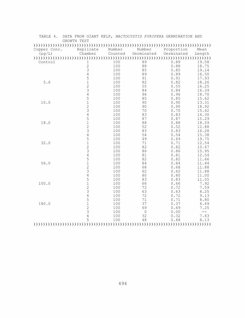
494

TABLE 4. DATA FROM GIANT KELP, MACTOCYSTIS PYRIFERA GERMINATION ANDGROWTH TEST

))))))))))))))))))))))))))))))))))))))))))))))))))))))))))))))))))))))))))Copper Conc. Replicate Number Number Proportion Mean (µg/L) Chamber Counted Germinated Germinated Length)))))))))))))))))))))))))))))))))))))))))))))))))))))))))))))))))))))))))) Control 1 100 89 0.89 19.58

2 100 88 0.88 18.753 100 85 0.85 19.144 100 89 0.89 16.505 100 91 0.91 17.93

5.6 1 100 82 0.82 18.262 100 55 0.55 16.253 100 84 0.84 16.394 100 96 0.96 18.705 100 85 0.85 15.62

10.0 1 100 90 0.90 13.312 100 90 0.90 18.923 100 70 0.70 15.624 100 83 0.83 14.305 100 87 0.87 15.29

18.0 1 100 88 0.88 18.592 100 52 0.52 12.883 100 83 0.83 16.284 100 54 0.54 15.385 100 49 0.49 19.75

32.0 1 100 71 0.71 12.542 100 82 0.82 10.673 100 86 0.86 15.954 100 81 0.81 12.545 100 82 0.82 11.66

56.0 1 100 84 0.84 11.442 100 68 0.68 11.883 100 62 0.62 11.884 100 80 0.80 11.005 100 83 0.83 11.55

100.0 1 100 66 0.66 7.922 100 72 0.72 7.593 100 63 0.63 8.254 100 72 0.72 9.135 100 71 0.71 8.80

180.0 1 100 37 0.37 6.492 100 69 0.69 7.253 100 0 0.00 --4 100 32 0.32 7.635 100 48 0.48 8.13

))))))))))))))))))))))))))))))))))))))))))))))))))))))))))))))))))))))))))

495

Figure 1. Flowchart for statistical analysis of giant kelp,Macrocystis pyrifera, germination data.

496

D ' 'n

i'1(Xi&X)2

17.13.2.4 Example of Analysis of Germination Data

17.12.2.4.1 This example used toxicity data from a giant kelp,Macrocystis pyrifera, germination and growth test performed withcopper. The response of interest is the proportion of germinatedspores, thus each replicate must be transformed by the arc sinesquare root transformation procedure described in Appendix B. The raw and transformed data, means and variances of thetransformed observations at each concentration including the control are listed in Table 5. A plot of the survival data isprovided in Figure 2.

17.13.2.5 Test for Normality

17.13.2.5.1 The first step of the test for normality is tocenter the observations by subtracting the mean of allobservations within a concentration from each observation in thatconcentration. The centered observations are listed in Table 6.

17.13.2.5.2 Calculate the denominator, D, of the test statistic:

Where: X&i = the ith centered observation

X& = the overall mean of the centered observations n = the total number of centered observations.

17.13.2.5.3 For this set of data, n = 40 X& = 1 (-0.002) = 0.000 40

D = 0.9281

17.13.2.5.4 Order the centered observations from smallest tolargest: X(1) # X(2) # ... # X(n)

497

TABLE 5. GIANT KELP, MACTOCYSTIS PYRIFERA GERMINATION DATA)))))))))))))))))))))))))))))))))))))))))))))))))))))))))))))))))))))))))) COPPER ARC SINECONCENTRATION REPLICATE RAW SQUARE ROOT MEAN (µg/L) CHAMBER DATA TRANSFORMED i Y& Si

2

)))))))))))))))))))))))))))))))))))))))))))))))))))))))))))))))))))))))))) Control 1 0.89 1.233 1 1.224 0.00114

2 0.88 1.2173 0.85 1.1734 0.89 1.2335 0.91 1.266

5.6 1 0.82 1.133 2 1.134 0.036702 0.55 0.8353 0.84 1.1594 0.96 1.3695 0.85 1.173

10.0 1 0.90 1.249 3 1.167 0.011522 0.90 1.2493 0.70 0.9914 0.83 1.1465 0.87 1.202

18.0 1 0.88 1.217 4 0.954 0.044232 0.52 0.8053 0.83 1.1464 0.54 0.8255 0.49 0.775

32.0 1 0.71 1.002 5 1.115 0.004662 0.82 1.1333 0.86 1.1874 0.81 1.1205 0.82 1.133

56.0 1 0.84 1.159 6 1.058 0.012722 0.68 0.9703 0.62 0.9074 0.80 1.1075 0.83 1.146

100.0 1 0.66 0.948 7 0.979 0.001912 0.72 1.0133 0.63 0.9174 0.72 1.0135 0.71 1.002

180.0 1 0.37 0.654 8 0.610 0.119142 0.69 0.9803 0.00 0.0504 0.32 0.6015 0.48 0.765

))))))))))))))))))))))))))))))))))))))))))))))))))))))))))))))))))))))))))

498

Figu

re 2

. Plo

t of g

erm

inat

ion

prop

ortio

ns o

f the

gia

nt k

elp,

M

acro

cyst

is p

yrife

ra, a

t eac

h tr

eatm

ent l

evel

.

499

TABLE 6. CENTERED OBSERVATIONS FOR SHAPIRO-WILK'S EXAMPLE)))))))))))))))))))))))))))))))))))))))))))))))))))))))))))))))))))))))))) Copper Concentration (µg/L) Rep Control 5.6 10.0 18.0 32.0 56.0 100.0 180.0)))))))))))))))))))))))))))))))))))))))))))))))))))))))))))))))))))))))))) 1 0.009 -0.001 0.082 0.263 -0.113 0.101 -0.031 0.044 2 -0.007 -0.299 0.082 -0.149 0.018 -0.088 0.034 0.370 3 -0.051 0.025 -0.176 0.192 0.072 -0.151 -0.062 -0.560 4 0.009 0.235 -0.021 -0.129 0.005 0.049 0.034 -0.009 5 0.042 0.039 0.035 -0.179 0.018 0.088 0.023 0.155))))))))))))))))))))))))))))))))))))))))))))))))))))))))))))))))))))))))))

TABLE 7. ORDERED CENTERED OBSERVATIONS FOR SHAPIRO-WILK'S EXAMPLE)))))))))))))))))))))))))))))))))))))))))))))))))))))))))))))))))))))))))) i X(i) i X(i)

)))))))))))))))))))))))))))))))))))))))))))))))))))))))))))))))))))))))))) 1 -0.560 21 0.018 2 -0.299 22 0.023 3 -0.179 23 0.025 4 -0.176 24 0.034 5 -0.151 25 0.034 6 -0.149 26 0.035 7 -0.129 27 0.039 8 -0.113 28 0.042 9 -0.088 29 0.044 10 -0.062 30 0.049 11 -0.051 31 0.072 12 -0.031 32 0.082 13 -0.021 33 0.082 14 -0.009 34 0.088 15 -0.007 35 0.101 16 -0.001 36 0.155 17 0.005 37 0.192 18 0.009 38 0.235 19 0.009 39 0.263 20 0.018 40 0.370))))))))))))))))))))))))))))))))))))))))))))))))))))))))))))))))))))))))))

Where X(i) is the ith ordered observation. These orderedobservations are listed in Table 7.

500

W '1D

[ 'k

i'1ai(X

(n&i%1)&X (i))]2

TABLE 8. COEFFICIENTS AND DIFFERENCES FOR SHAPIRO-WILK'S EXAMPLE)))))))))))))))))))))))))))))))))))))))))))))))))))))))))))))))))))))))))) i ai X(n-i+1) - X(i) )))))))))))))))))))))))))))))))))))))))))))))))))))))))))))))))))))))))))) 1 0.3964 0.930 X(40) - X(1) 2 0.2737 0.562 X(39) - X(2) 3 0.2368 0.414 X(38) - X(3) 4 0.2098 0.368 X(37) - X(4) 5 0.1878 0.306 X(36) - X(5) 6 0.1691 0.250 X(35) - X(6) 7 0.1526 0.217 X(34) - X(7) 8 0.1376 0.195 X(33) - X(8) 9 0.1237 0.170 X(32) - X(9) 10 0.1108 0.134 X(31) - X(10) 11 0.0986 0.100 X(30) - X(11) 12 0.0870 0.075 X(29) - X(12) 13 0.0759 0.063 X(28) - X(13) 14 0.0651 0.048 X(27) - X(14) 15 0.0546 0.042 X(26) - X(15) 16 0.0444 0.035 X(25) - X(16) 17 0.0343 0.029 X(24) - X(17) 18 0.0244 0.016 X(23) - X(18) 19 0.0146 0.014 X(22) - X(19) 20 0.0049 0.000 X(21) - X(20) ))))))))))))))))))))))))))))))))))))))))))))))))))))))))))))))))))))))))))

17.13.2.5.5 From Table 4, Appendix B, for the number ofobservations, n, obtain the coefficients a1, a2,...., ak where kis n/2 if n is even and (n-1)/2 if n is odd. For the data inthis example, n = 40 and k = 20. The ai values are listed inTable 8.

17.13.2.5.6 Compute the test statistic, W, as follows:

The differences X(n-i+1) - X(i) are listed in Table 8. For this datain this example:

W = 1 (0.9230)2 = 0.918 0.9281

501

TABLE 9. ASSIGNING RANKS TO THE CONTROL AND 5.6 µg/LCONCENTRATION LEVEL FOR STEEL'S MANY-ONE RANK TEST

)))))))))))))))))))))))))))))))))))))))))))))))))))))))))))))))))))))) Transformed Proportion Rank Germinated Concentration )))))))))))))))))))))))))))))))))))))))))))))))))))))))))))))))))))))) 1 0.835 5.6 µg/L 2 1.133 5.6 µg/L 3 1.159 5.6 µg/L 4.5 1.173 5.6 µg/L 4.5 1.173 Control 6 1.217 Control 7.5 1.233 Control 7.5 1.233 Control 9 1.266 Control 10 1.369 5.6 µg/L ))))))))))))))))))))))))))))))))))))))))))))))))))))))))))))))))))))))

TABLE 10. TABLE OF RANKS1

)))))))))))))))))))))))))))))))))))))))))))))))))))))))))))))))))))))))))) Concentration (µg/L) ))))))))))))))))))))))))))))))Rep. Control 5.6 10.0)))))))))))))))))))))))))))))))))))))))))))))))))))))))))))))))))))))))))) 1 1.233(7.5,6.5,8.5,8.5,8.5,8.5,8.5) 1.133(2) 1.249(8.5) 2 1.217(6,5,6.5,7,7,7,7) 0.835(1) 1.249(8.5) 3 1.173(4.5,3,5,5,6,6,6) 1.159(3) 0.991(1) 4 1.233(7.5,6.5,8.5,8.5,8.5,8.5,8.5) 1.369(10) 1.146(2) 5 1.266(9,10,10,10,10,10,10) 1.173(4.5) 1.202(4)-------------------------------------------------------------------------- Concentration (µg/L) (Continued) )))))))))))))))))))))))))))))))))))))))))))))))))))))))))))))))Rep. 18.0 32.0 56.0 100.0 180.0)))))))))))))))))))))))))))))))))))))))))))))))))))))))))))))))))))))))))) 1 1.217(6.5) 1.002(1) 1.159(5) 0.948(2) 0.654(3) 2 0.805(2) 1.133(3.5) 0.970(2) 1.013(4.5) 0.980(5) 3 1.146(4) 1.187(6) 0.907(1) 0.917(1) 0.050(1) 4 0.825(3) 1.120(2) 1.107(3) 1.013(4.5) 0.601(2) 5 0.775(1) 1.133(3.5) 1.146(4) 1.002(3) 0.765(4)))))))))))))))))))))))))))))))))))))))))))))))))))))))))))))))))))))))))))1Control ranks are given in the order of the concentration with which they were ranked.

502

17.13.2.5.7 The decision rule for this test is to compare W ascalculated in Subsection 5.6 with the critical value found inTable 6, Appendix B. If the computed W is less than the criticalvalue, conclude that the data are not normally distributed. Forthis set of data, the critical value at a significance level of0.01 and n = 40 observations is 0.919. Since W = 0.918 is lessthan the critical value, conclude that the data are not normallydistributed.

17.13.2.5.8 Since the data do not meet the assumption ofnormality, Steel's Many-one Rank Test will be used to analyze thegermination data.

17.13.2.6 Steel's Many-one Rank Test 17.13.2.6.1 For each control and concentration combination,combine the data and arrange the observations in order of sizefrom smallest to largest. Assign the ranks (1, 2, ... , 10) tothe ordered observations with a rank of 1 assigned to thesmallest observation, rank of 2 assigned to the next largerobservation, etc. If ties occur when ranking, assign the averagerank to each tied observation. 17.13.2.6.2 An example of assigning ranks to the combined datafor the control and 5.6 µg/L copper concentration is given inTable 9. This ranking procedure is repeated for eachcontrol/concentration combination. The complete set of rankingsis summarized in Table 10. The ranks are then summed for eachconcentration level, as shown in Table 11.

17.13.2.6.3 For this example, determine if the survival in anyof the concentrations is significantly lower than the survival inthe control. If this occurs, the rank sum at that concentrationwould be significantly lower than the rank sum of the control. Thus compare the rank sums for the survival at each of thevarious concentration levels with some "minimum" or critical ranksum, at or below which the survival would be consideredsignificantly lower than the control. At a significance level of0.05, the minimum rank sum in a test with seven concentrations(excluding the control) and five replicates is 16 (See Table 5,Appendix E).

503

TABLE 11. RANK SUMS ))))))))))))))))))))))))))))))))))))))))))))))))))))))))) Concentration Rank Sum ))))))))))))))))))))))))))))))))))))))))))))))))))))))))) 5.6 20.5 10.0 24.0 18.0 16.5 32.0 16.0 56.0 15.0 100.0 15.0 180.0 15.0

17.13.2.6.4 Since the rank sum for the 32.0 µg/L concentrationis equal to the critical value and the rank sums for the 56.0,100.0 and 180.0 µg/L concentrations are less than the criticalvalue, the germination proportions in those concentrations areconsidered significantly less than that in the control. Hence,the NOEC and the LOEC are considered to be 18.0 µg/L and 32.0µg/L, respectively.

17.13.2.7 Calculation of the ICp

17.13.2.7.1 The germination data from Table 4 and Figure 2 areutilized in this example. As can be seen from the figure, theobserved means are not monotonically non-increasing with respectto concentration. Therefore, the means must be smoothed prior tocalculating the IC.

17.13.2.7.2 Starting with the observed control mean, Y1 = 0.884is less than the observed mean for the lowest effluentconcentration, Y2 = 0.804, so set M1 = 0.884.

17.13.2.7.3 Comparing Y2 to Y3 = 0.840, we see that Y2 is lessthan Y3.

17.13.2.7.4 Calculate the smoothed means: M2 = M3 = (Y2 + Y3)/2 = 0.822

504

ICp ' Cj%[M1(1&p/100)&Mj](C(j%1)&Cj)

(M(j%1)&Mj)

17.13.2.7.5 Since M3 is larger than Y4 = 0.652, set M4 = 0.652. Since Y5 = 0.804 is larger than M4, these means must be smoothed.

17.13.2.7.6 Calculate the smoothed means: M4 = M5 = (M4 + Y5)/2 = 0.728. 17.13.2.7.7 Since Y6 = 0.754 is larger than M5, average Y6 withthe two previous concentrations: M4 = M5 = M6 = (M4 + M5 + Y6)/3 = 0.737.

17.13.2.7.8 Since M6 > Y7 = 0.688 > Y8 = 0.372, set M7 = 0.688and M8 = 0.372. Table 12 contains the smoothed means andFigure 3 gives a plot of the smoothed means and the interpolatedresponse curve.

17.13.2.7.9 An IC25 can be estimated using the LinearInterpolation Method. A 25% reduction in germination, comparedto the controls, would result in a mean germination of 0.663,where M1(1-p/100) = 0.884(1-25/100). Examining the smoothedmeans and their associated concentrations (Table 12), theresponse, 0.663, is bracketed by C7 = 100.0 µg/L and C8 = 180.0µg/L.

17.13.2.7.10 Using the equation in Section 4.2 from Appendix L,the estimate of the IC25 is calculated as follows:

IC25 = 100.0 + [0.884(1 - 25/100) - 0.688] (180.0 - 100.0) S))))))))))))))Q (0.372 - 0.688) = 106.3 µg/L.

17.13.2.7.11 When the ICPIN program was used to analyze this setof data, requesting 80 resamples, the estimate of the IC25 was106.3291 µg/L. The empirical 95.0% confidence interval for thetrue mean was 94.6667 µg/L to 117.0588 µg/L. The computerprogram output for the IC25 for this data set is shown inFigure 4.

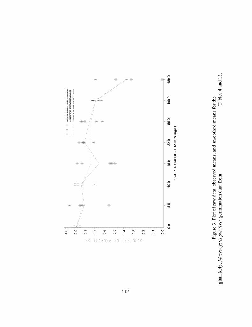
505

Figu

re 3

. Plo

t of r

aw d

ata,

obs

erve

d m

eans

, and

sm

ooth

ed m

eans

for t

he

gian

t kel

p, M

acro

cyst

is p

yrife

ra, g

erm

inat

ion

data

from

T

able

s 4

and

13.

506

Conc. ID 1 2 3 4 5 6 7 8----------------------------------------------------Conc. Tested 0 5.6 10 18 32 56 100 180----------------------------------------------------Response 1 .89 .82 .90 .88 .71 .84 .66 .37Response 2 .88 .55 .90 .52 .82 .68 .72 .69Response 3 .85 .84 .70 .83 .86 .62 .63 0Response 4 .89 .96 .83 .54 .81 .80 .72 .32Response 5 .91 .85 .87 .49 .82 .83 .71 .48----------------------------------------------------*** Inhibition Concentration Percentage Estimate ***Toxicant/Effluent: CopperTest Start Date: Test Ending Date: Test Species: Giant Kelp, Macrocystis pyriferaTest Duration: 48 hoursDATA FILE: kelpgerm.icpOUTPUT FILE: kelpgerm.i25-----------------------------------------------------------------------Conc. Number Concentration Response Std. Pooled ID Replicates ug/L Means Dev. Response Means----------------------------------------------------------------------- 1 5 0.000 0.884 0.022 0.884 2 5 5.600 0.804 0.152 0.822 3 5 10.000 0.840 0.083 0.822 4 5 18.000 0.652 0.187 0.737 5 5 32.000 0.804 0.056 0.737 6 5 56.000 0.754 0.098 0.737 7 5 100.000 0.688 0.041 0.688 8 5 180.000 0.372 0.252 0.372-----------------------------------------------------------------------The Linear Interpolation Estimate: 106.3291 Entered P Value: 25-----------------------------------------------------------------------Number of Resamplings: 80The Bootstrap Estimates Mean: 105.8680 Standard Deviation: 5.6981Original Confidence Limits: Lower: 94.6667 Upper: 117.0588Expanded Confidence Limits: Lower: 88.8354 Upper: 122.4237Resampling time in Seconds: 0.28 Random_Seed: 390692880

Figure 4. ICPIN program output for the IC25.

507

17.13.3 EXAMPLE OF ANALYSIS OF GIANT KELP, MACROCYSTIS PYRIFERA,GROWTH DATA

17.13.3.1 Formal statistical analysis of the growth data isoutlined in Figure 5. The response used in the statistical analysis is mean germ-tube length per replicate. An IC25 can becalculated for the growth data via a point estimation technique(see Section 9, Chronic Toxicity Test Endpoints and DataAnalysis). Hypothesis testing can be used to obtain the NOEC andLOEC for growth.

17.13.3.2 The statistical analysis using hypothesis testsconsists of a parametric test, Dunnett's Procedure, and anonparametric test, Steel's Many-one Rank Test. The underlyingassumptions of the Dunnett's Procedure, normality and homogeneityof variance, are formally tested. The test for normality is theShapiro-Wilk's Test and Bartlett's Test is used to test forhomogeneity of variance. If either of these tests fails, thenonparametric test, Steel's Many-one Rank Test, is used todetermine the NOEC and LOEC endpoints. If the assumptions ofDunnett's Procedure are met, the endpoints are determined by theparametric test.

17.13.3.3 Additionally, if unequal numbers of replicates occuramong the concentration levels tested, there are parametric andnonparametric alternative analyses. The parametric analysis is at test with the Bonferroni adjustment. The Wilcoxon Rank SumTest with the Bonferroni adjustment is the nonparametric alternative. For detailed information on the Bonferroniadjustment, see Appendix D.

17.13.3.4 The data, mean and variance of the observations ateach concentration including the control for this example arelisted in Table 13. A plot of the data is provided in Figure 6.

17.13.3.5 Test for Normality

17.13.3.5.1 The first step of the test for normality is tocenter the observations by subtracting the mean of allobservations within a concentration from each observation in thatconcentration. The centered observations are listed in Table 14.

508

Figure 5. Flowchart for statistical analysis of giant kelp,Macrocystis pyrifera, growth data.

509

TABLE 13. GIANT KELP, MACROCYSTIS PYRIFERA, GROWTH DATA)))))))))))))))))))))))))))))))))))))))))))))))))))))))))))))))))))))))))) Copper Concentration (µg/L)

)))))))))))))))))))))))))))))))))))))))))))))))))))))))) Rep Control 5.60 10.0 18.0 32.0 56.0 100.0 180.0)))))))))))))))))))))))))))))))))))))))))))))))))))))))))))))))))))))))))) 1 19.58 18.26 13.31 18.59 12.54 11.44 7.92 6.49 2 18.75 16.25 18.92 12.88 10.67 11.88 7.59 7.25 3 19.14 16.39 15.62 16.28 15.95 11.88 8.25 -- 4 16.50 18.70 14.30 15.38 12.54 11.00 9.13 7.63 5 17.93 15.62 15.29 19.75 11.66 11.55 8.80 8.13))))))))))))))))))))))))))))))))))))))))))))))))))))))))))))))))))))))))))))Mean(Y&i) 18.38 17.04 15.49 16.58 12.67 11.55 8.34 7.38Si2 1.473 1.827 4.498 7.327 3.953 0.133 0.396 0.478

i 1 2 3 4 5 6 7 8))))))))))))))))))))))))))))))))))))))))))))))))))))))))))))))))))))))))))))

TABLE 14. CENTERED OBSERVATIONS FOR SHAPIRO-WILK'S EXAMPLE)))))))))))))))))))))))))))))))))))))))))))))))))))))))))))))))))))))))))) Copper Concentration (µg/L) Rep Control 5.6 10.0 18.0 32.0 56.0 100.0 180.0)))))))))))))))))))))))))))))))))))))))))))))))))))))))))))))))))))))))))) 1 1.20 1.22 -2.18 2.01 -0.13 -0.11 -0.42 -0.89 2 0.37 -0.79 3.43 -3.70 -2.00 0.33 -0.75 -0.13 3 0.76 -0.65 0.13 -0.30 3.28 0.33 -0.09 -- 4 -1.88 1.66 -1.19 -1.20 -0.13 -0.55 0.79 0.25 5 -0.45 -1.42 -0.20 3.17 -1.01 0.00 0.46 0.75))))))))))))))))))))))))))))))))))))))))))))))))))))))))))))))))))))))))))

D ' 'n

i'1(Xi&X)2

17.13.3.5.2 Calculate the denominator, D, of the statistic:

Where: Xi = the ith centered observation X& = the overall mean of the centered observations

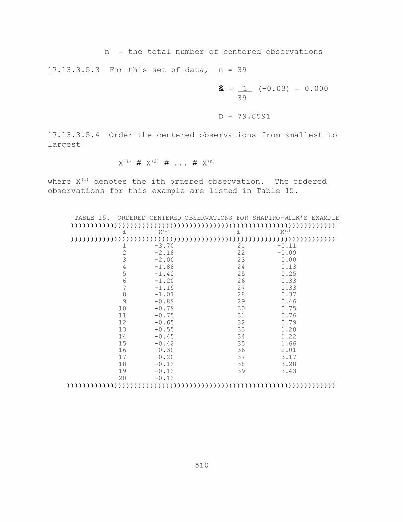
510

TABLE 15. ORDERED CENTERED OBSERVATIONS FOR SHAPIRO-WILK'S EXAMPLE ))))))))))))))))))))))))))))))))))))))))))))))))))))))))))))))))))) i X(i) i X(i)

))))))))))))))))))))))))))))))))))))))))))))))))))))))))))))))))))) 1 -3.70 21 -0.11 2 -2.18 22 -0.09 3 -2.00 23 0.00 4 -1.88 24 0.13 5 -1.42 25 0.25 6 -1.20 26 0.33 7 -1.19 27 0.33 8 -1.01 28 0.37 9 -0.89 29 0.46 10 -0.79 30 0.75 11 -0.75 31 0.76 12 -0.65 32 0.79 13 -0.55 33 1.20 14 -0.45 34 1.22 15 -0.42 35 1.66 16 -0.30 36 2.01 17 -0.20 37 3.17 18 -0.13 38 3.28 19 -0.13 39 3.43 20 -0.13 ))))))))))))))))))))))))))))))))))))))))))))))))))))))))))))))))))))

n = the total number of centered observations

17.13.3.5.3 For this set of data, n = 39

X& = 1 (-0.03) = 0.000 39

D = 79.8591

17.13.3.5.4 Order the centered observations from smallest tolargest

X(1) # X(2) # ... # X(n)

where X(i) denotes the ith ordered observation. The orderedobservations for this example are listed in Table 15.

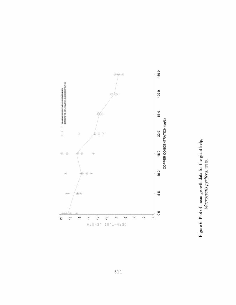
511

Figu

re 6

. Plo

t of m

ean

grow

th d

ata

for t

he g

iant

kel

p,M

acro

cyst

is p

yrife

ra, t

ests

.

512

W '1D

[ 'k

i'1ai(X

(n&i%1)&X (i))]2

TABLE 16. COEFFICIENTS AND DIFFERENCES FOR SHAPIRO-WILK'S EXAMPLE)))))))))))))))))))))))))))))))))))))))))))))))))))))))))))))))))))))))))) i ai X(n-i+1) - X(i) )))))))))))))))))))))))))))))))))))))))))))))))))))))))))))))))))))))))))) 1 0.3989 7.13 X(39) - X(1) 2 0.2755 5.46 X(38) - X(2) 3 0.2380 5.17 X(37) - X(3) 4 0.2104 3.89 X(36) - X(4) 5 0.1880 3.08 X(35) - X(5) 6 0.1689 2.42 X(34) - X(6) 7 0.1520 2.39 X(33) - X(7) 8 0.1366 1.80 X(32) - X(8) 9 0.1225 1.65 X(31) - X(9) 10 0.1092 1.54 X(30) - X(10) 11 0.0967 1.21 X(29) - X(11) 12 0.0848 1.02 X(28) - X(12) 13 0.0733 0.88 X(27) - X(13) 14 0.0622 0.78 X(26) - X(14) 15 0.0515 0.67 X(25) - X(15) 16 0.0409 0.43 X(24) - X(16) 17 0.0305 0.20 X(23) - X(17) 18 0.0203 0.04 X(22) - X(18) 19 0.0101 0.02 X(21) - X(19) ))))))))))))))))))))))))))))))))))))))))))))))))))))))))))))))))))))))))))

17.13.3.5.5 From Table 4, Appendix B, for the number ofobservations, n, obtain the coefficients a1, a2, ... ak where k isn/2 if n is even and (n-1)/2 if n is odd. For the data in thisexample, n = 39 and k = 19. The ai values are listed inTable 16.

17.13.3.5.6 Compute the test statistic, W, as follows:

The differences X(n-i+1) - X(i) are listed in Table 16. For this setof data:

W = 1 (8.7403)2 = 0.957 79.8591

513

B '

[( 'P

i'1Vi) 1n S2 & '

P

i'1Vi 1n S 2

i ]

C

17.13.3.5.7 The decision rule for this test is to compare W ascalculated in Subsection 5.6 to a critical value found inTable 6, Appendix B. If the computed W is less than the criticalvalue, conclude that the data are not normally distributed. Forthis set of data, the critical value at a significance level of0.01 and n = 39 observations is 0.917. Since W = 0.957 isgreater than the critical value, conclude that the data arenormally distributed.

17.13.3.6 Test for Homogeneity of Variance

17.13.3.6.1 The test used to examine whether the variation inmean weight of the mysids is the same across all concentrationlevels including the control, is Bartlett's Test (Snedecor andCochran, 1980). The test statistic is as follows:

Where: Vi = degrees of freedom for each copper concentrationand control, Vi = (ni - 1)

p = number of concentration levels including thecontrol

ln = loge

i = 1, 2, ..., p where p is the number ofconcentrations including the control

ni = the number of replicates for concentration i.

S2 '

( 'P

i'1ViS

2i )

'P

i'1Vi

C ' 1% [3(p&1)]&1[ 'P

i'11/Vi& ( '

P

i'1Vi)

&1]

514

B ' [(31) ln(2.5761) & 'P

i'1Vi ln(S 2

i )] / 1.0977

TABLE 17. ANOVA TABLE Source df Sum of Squares Mean Square(MS) (SS) (SS/df) 2 Between p - 1 SSB SB = SSB/(p-1) 2 Within N - p SSW SW = SSW/(N-p)

Total N - 1 SST

17.13.3.6.2 For the data in this example (See Table 13), allconcentrations including the control have five replicates exceptthe 180 µg/L concentration which has four replicates (ni = 5 fori = 1 - 7; n8 = 4). Thus, Vi = 4 for i = 1 - 7 and V8 = 3.

17.13.3.6.3 Bartlett's statistic is therefore:

= [31(0.9463) - [4ln(1.4729) + ... + 3ln(0.4780)] / 1.0977 = [29.3353 - 9.4481] / 1.0977 = 18.12

17.13.3.6.4 B is approximately distributed as chi-square with p- 1 degrees of freedom, when the variances are in fact the same. Therefore, the appropriate critical value for this test, at asignificance level of 0.01 with seven degrees of freedom, is18.48. Since B = 18.12 is less than the critical value, concludethat the variances are not different. 17.13.3.7 t Test with Bonferroni's Adjustment

17.13.3.7.1 To obtain an estimate of the pooled variance for thet test with Bonferroni's adjustment, construct an ANOVA table asdescribed in Table 17.

Where: p = number of concentration levels including the control

515

N = total number of observations n1 + n2 ... + np

ni = number of observations in concentration i

Between Sum of SquaresSSB ' 'P

i'1T 2

i /ni&G 2/N

Total Sum of SquaresSST ' 'P

i'1'ni

j'1Y

2ij &G 2/N

Within Sum of Squares SSW ' SST&SSB

G = the grand total of all sample observations,

G ' 'P

i'1Ti

Ti = the total of the replicate measurements forconcentration i

Yij = the jth observation for concentration i(represents the mean length of the germ-tubes forconcentration i in test chamber j)

17.13.3.7.2 For the data in this example:

n1 = n2 = n3 = n4 = n5 = n6 = n7 = 5; n8 = 4

N = 39

T1 = Y11 + Y12 + Y13 + Y14 + Y15 = 91.90 T2 = Y21 + Y22 + Y23 + Y24 + Y25 = 85.22 T3 = Y31 + Y32 + Y33 + Y34 + Y35 = 77.44 T4 = Y41 + Y42 + Y43 + Y44 + Y45 = 82.88 T5 = Y51 + Y52 + Y53 + Y54 + Y55 = 63.36 T6 = Y61 + Y62 + Y63 + Y64 + Y65 = 57.75 T7 = Y71 + Y72 + Y73 + Y74 + Y75 = 41.69 T8 = Y81 + Y82 + Y83 + Y84 = 29.50

G = T1 + T2 + T3 + T4 + T5 + T6 + T7 + T8 = 529.74

SSB ' 'P

i'1T 2

i /ni&G 2/N

516

TABLE 18. ANOVA TABLE FOR THE t TEST WITH BONFERRONI'S ADJUSTMENT EXAMPLE

)))))))))))))))))))))))))))))))))))))))))))))))))))))))))))))))))))))))))) Source df Sum of Squares Mean Square (MS) (SS) (SS/df) )))))))))))))))))))))))))))))))))))))))))))))))))))))))))))))))))))))))))) Between 7 554.406 79.201 Within 31 79.859 2.576 )))))))))))))))))))))))))))))))))))))))))))))))))))))))))))))))))))))))))) Total 38 634.265 ))))))))))))))))))))))))))))))))))))))))))))))))))))))))))))))))))))))))))

ti '(Y1 & Y i)

Sw (1/n1) % (1/ni)

= 7749.905 - (529.74)2 = 554.406 39

SST ' 'P

i'1'ni

j'1Y

2ij &G 2/N

= 7829.764 - (529.74)2 = 634.265 39

= 634.265 - 554.406 = 79.859 SSW ' SST&SSB

SB2 = SSB/(p-1) = 554.406/(8-1) = 79.201

SW2 = SSW/(N-p) = 79.859/(39-8) = 2.576

17.13.3.7.3 Summarize these calculations in the ANOVA table(Table 18).

17.13.3.7.4 To perform the individual comparisons, calculate thet statistic for each concentration, and control combination asfollows:

517

t2 '(18.38 & 17.04)

[1.605 (1/5)% (1/5) ]

TABLE 19. CALCULATED t VALUES )))))))))))))))))))))))))))))))))))))))))))))))))))))))))))))))))))))))))) Concentration (µg/L) i ti )))))))))))))))))))))))))))))))))))))))))))))))))))))))))))))))))))))))))) 5.6 2 1.320 10.0 3 2.847 18.0 4 1.773 32.0 5 5.625 56.0 6 6.728 100.0 7 9.891 180.0 8 10.836))))))))))))))))))))))))))))))))))))))))))))))))))))))))))))))))))))))))))

Where: Y&i = mean length for concentration i

Y&1 = mean length for the control

SW = square root of the within mean square

n1 = number of replicates for the control

ni = number of replicates for concentration i

17.13.3.7.5 Table 19 includes the calculated t values for eachconcentration and control combination. In this example,comparing the 5.6 µg/L concentration with the control, thecalculation is as follows:

= 1.320

17.13.3.7.6 Since the purpose of this test is to detect asignificant reduction in mean length, a one-sided test isappropriate. The critical value for this one-sided test is foundin Table 5, Appendix D. For an overall alpha level of 0.05, 31degrees of freedom for error and seven concentrations (excludingthe control) the approximate critical value is 2.597. The meanweight for concentration "i" is considered significantly lessthan the mean weight for the control if ti is greater than thecritical value. Therefore, the 10.0 µg/L, 32 µg/L, 56.0 µg/L,

518

100.0 µg/L, 180.0 µg/L concentrations have significantly lowermean length than the control. Because the 10.0 µg/Lconcentration shows signigicantly lower mean length than thecontrol while the higher 18.0 µg/L concentration does not, thesetest results are considered to have an anomalous dose-responserelationship and it is recommended that the test be repeated. Ifan NOEC and LOEC must be determined for this test, the lowestconcentration with significant growth impairment versus thecontrol is considered to the LOEC for growth. Thus, for thistest, the NOEC and LOEC would be 5.6 µg/L and 10.0 µg/L,respectively.

17.13.3.8 Calculation of the ICp

17.13.3.8.1 The growth data from Table 13 and Figure 3 areutilized in this example. As can be seen in the figure, theobserved means are not monotonically non-increasing with respectto concentration. Therefore, the means must be smoothed prior tocalculating the IC

17.13.3.8.2 Starting with the observed control mean, Y1 = 18.38is greater than the observed mean for the lowest copperconcentration, Y2 = 17.044, so set M1 = 18.38. Likewise, Y2 isgreater than the observed mean for the next copper concentration,Y3 = 15.488, so set M2 = 17.044.

17.13.3.8.3 Comparing Y3 to Y4 = 16.576, we see that Y3 is lessthan Y4.

17.13.3.8.4 Calculate the smoothed means: M3 = M4 = (Y3 + Y4)/2 = 16.032

17.13.3.8.5 Since M4 > Y5 = 12.672 > Y6 = 11.550 > Y7 = 8.338 > Y8

= 7.375, set M5 = 12.672, M6 = 11.550, M7 = 8.338 and M8 = 7.375. Table 20 contains the smoothed means and Figure 7 gives a plot ofthe smoothed response curve.

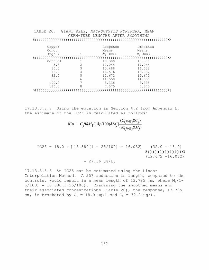
519

TABLE 20. GIANT KELP, MACROCYSTIS PYRIFERA, MEAN GERM-TUBE LENGTHS AFTER SMOOTHING S)))))))))))))))))))))))))))))))))))))))))))))))))))))))))))))))))Q

Copper Response Smoothed Conc. Means Means (µg/L) i Y&i (mm) Mi (mm) S)))))))))))))))))))))))))))))))))))))))))))))))))))))))))))))))))Q Control 1 18.380 18.380 5.6 2 17.044 17.044 10.0 3 15.488 16.032 18.0 4 16.576 16.032 32.0 5 12.672 12.672 56.0 6 11.550 11.550 100.0 7 8.338 8.338 180.0 8 7.375 7.375 S)))))))))))))))))))))))))))))))))))))))))))))))))))))))))))))))))Q

ICp ' Cj%[M1(1&p/100)&Mj](C(j%1)&Cj)

(M(j%1)&Mj)

17.13.3.8.7 Using the equation in Section 4.2 from Appendix L,the estimate of the IC25 is calculated as follows:

IC25 = 18.0 + [18.380(1 - 25/100) - 16.032] (32.0 - 18.0) S))))))))))))))Q (12.672 -16.032) = 27.36 µg/L.

17.13.3.8.6 An IC25 can be estimated using the LinearInterpolation Method. A 25% reduction in length, compared to thecontrols, would result in a mean length of 13.785 mm, where M1(1-p/100) = 18.380(1-25/100). Examining the smoothed means andtheir associated concentrations (Table 20), the response, 13.785mm, is bracketed by C4 = 18.0 µg/L and C5 = 32.0 µg/L.

520

Figu

re 7

. Plo

t of r

aw d

ata,

obs

erve

d m

eans

, and

sm

ooth

ed m

eans

for t

he g

iant

K

elp,

Mac

rocy

stis

pyr

ifera

, gro

wth

dat

a fr

om T

able

s 13

and

20.

521

17.13.3.8.8 When the ICPIN program was used to analyze this setof data, requesting 80 resamples, the estimate of the IC25 was27.3625 µg/L. The empirical 95.0% confidence interval for thetrue mean was 20.8734 µg/L to 42.3270 µg/L. The computer programoutput for the IC25 for this data set is shown in Figure 8.

17.14 PRECISION AND ACCURACY

17.14.1 PRECISION

17.14.1.1 Single-Laboratory Precision

17.14.1.1.1 Single-laboratory precision data for the giant kelp48-hour test method with the reference toxicants copper chlorideand sodium azide with natural seawater are provided in Tables 21-22. The coefficient of variation (CV) of the germination EC50susing copper was 38.8%; the CV of the germ-tube length IC40susing copper was 32.9% (Table 21). The coefficient of variation(CV) of the germination EC50s using azide was 36.7%; the CV ofthe germ-tube length IC25s using azide was 30.8%, the CV of thegerm-tube length IC50s using azide was 28.4% (Table 22).

17.14.1.2 Multi-laboratory Precision

17.14.1.2.1 Multi-laboratory precision data for the kelp 48-hourtest method with the reference toxicant copper chloride areprovided in Table 23. The coefficient of variation of the IC50sfor the germ-tube length endpoint ranged between 8.4% and 55.5%using copper chloride. The coefficient of variation of the IC50sfor the germination endpoint ranged between >1.1% and 67.6% usingcopper chloride.

17.14.2 ACCURACY

17.14.2.1 The accuracy of toxicity tests cannot be determined.

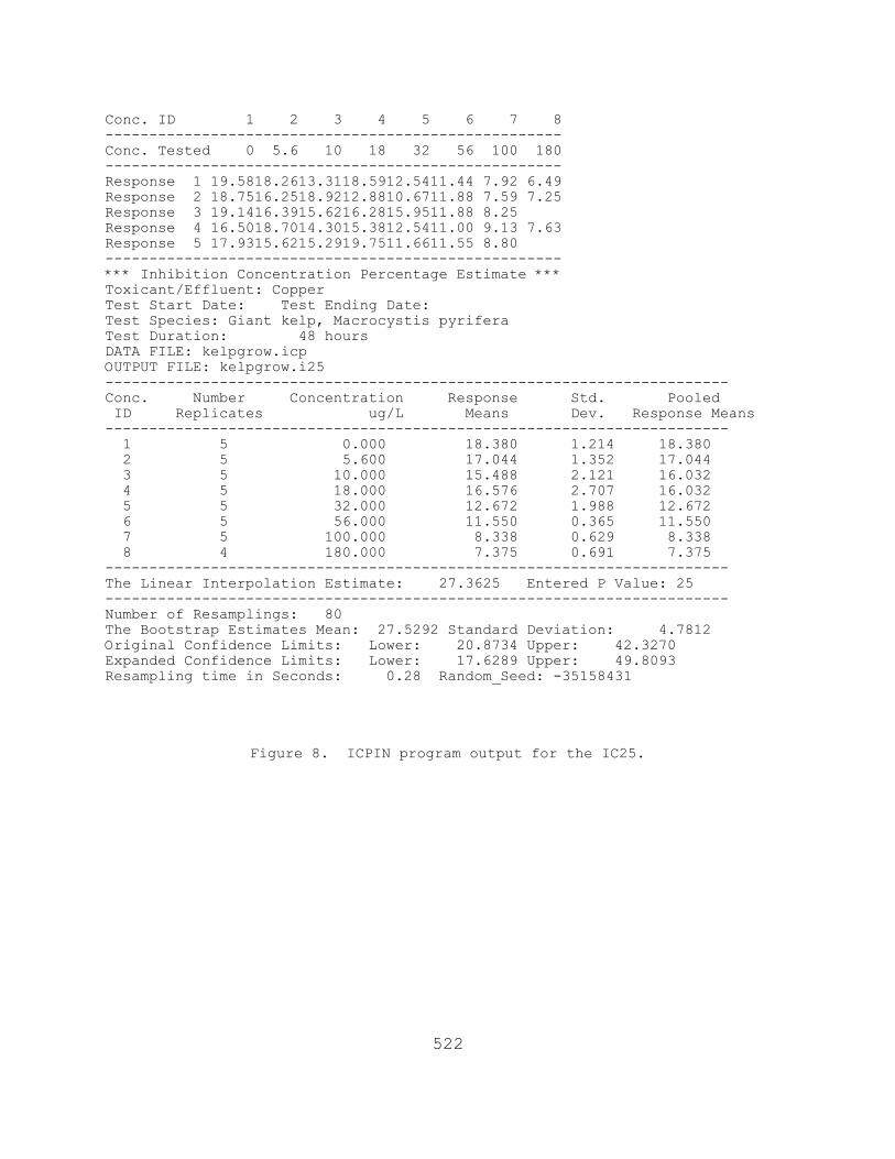
522

Conc. ID 1 2 3 4 5 6 7 8----------------------------------------------------Conc. Tested 0 5.6 10 18 32 56 100 180----------------------------------------------------Response 1 19.5818.2613.3118.5912.5411.44 7.92 6.49Response 2 18.7516.2518.9212.8810.6711.88 7.59 7.25Response 3 19.1416.3915.6216.2815.9511.88 8.25 Response 4 16.5018.7014.3015.3812.5411.00 9.13 7.63Response 5 17.9315.6215.2919.7511.6611.55 8.80 ----------------------------------------------------*** Inhibition Concentration Percentage Estimate ***Toxicant/Effluent: CopperTest Start Date: Test Ending Date: Test Species: Giant kelp, Macrocystis pyriferaTest Duration: 48 hoursDATA FILE: kelpgrow.icpOUTPUT FILE: kelpgrow.i25-----------------------------------------------------------------------Conc. Number Concentration Response Std. Pooled ID Replicates ug/L Means Dev. Response Means----------------------------------------------------------------------- 1 5 0.000 18.380 1.214 18.380 2 5 5.600 17.044 1.352 17.044 3 5 10.000 15.488 2.121 16.032 4 5 18.000 16.576 2.707 16.032 5 5 32.000 12.672 1.988 12.672 6 5 56.000 11.550 0.365 11.550 7 5 100.000 8.338 0.629 8.338 8 4 180.000 7.375 0.691 7.375-----------------------------------------------------------------------The Linear Interpolation Estimate: 27.3625 Entered P Value: 25-----------------------------------------------------------------------Number of Resamplings: 80The Bootstrap Estimates Mean: 27.5292 Standard Deviation: 4.7812Original Confidence Limits: Lower: 20.8734 Upper: 42.3270Expanded Confidence Limits: Lower: 17.6289 Upper: 49.8093Resampling time in Seconds: 0.28 Random_Seed: -35158431

Figure 8. ICPIN program output for the IC25.

523

TABLE 21. SINGLE LABORATORY PRECISION OF THE GIANT KELP,MACROCYSTIS PYRIFERA GERMINATION AND GERM-TUBE LENGTHTEST WITH COPPER (CU FG/L) CHLORIDE AS THE REFERENCETOXICANT

Test Number Germ-Tube LengthNOEC IC40

GerminationNOEC EC50

12345

<5.6 122.710.0 43.118.0 70.7 5.6 88.032.0 124.7

10.0 67.518.0 73.518.0 124.356.0 101.656.0 122.9

MeanCV

89.8 38.8%

90.7 32.9%

Data from Anderson et al., 1994

TABLE 22. SINGLE LABORATORY PRECISION OF THE GIANT KELP,MACROCYSTIS PYRIFERA GERMINATION AND GERM-TUBE LENGTHTEST WITH SODIUM AZIDE (MG/L) AS THE REFERENCETOXICANT

Test Date Germ-Tube LengthNOEC IC25 IC50

GerminationNOEC EC50

2/11/922/18/926/29/927/07/927/15/927/16/927/22/9210/09/927/02/92

18.0 39.5 133.718.0 34.1 96.532.0 57.5 142.210.0 33.1 92.518.0 42.8 138.9 5.6 25.0 68.410.0 30.2 80.6 5.6 25.1 80.010.0 24.8 80.1

18.0 52.332.0 72.632.0 132.110.0 79.218.0 117.810.0 48.318.0 62.4 5.6 60.318.0 84.0

MeanCV

34.7 101.4 30.8% 28.4%

78.8 36.7%

Data from Hunt et al., 1991

524

TABLE 23. MULTI-LABORATORY PRECISION OF THE GIANT KELP,MACROCYSTIS PYRIFERA GERMINATION AND GERM-TUBE LENGTHTEST PERFORMED WITH COPPER CHLORIDE (µG/L) AS THEREFERENCE TOXICANT

Lab Germ-tube lengthNOEC IC40

GerminationNOEC EC50

CVGerm-tube

CVGermination

March 1990 123

5.6 122.732.0 117.818.0 104.1

10.0 46.932.0 46.232.0 *

8.4% >1.1%

May 1990 123

10.0 43.1<5.6 99.118.0 68.7

18.0 112.032.0 164.218.0 67.9

39.9% 59.3%

May 1990 123

18.0 70.718.0 91.332.0 134.2

18.0 112.056.0 64.532.0 158.0

45.3% nc

December1990

12

5.6 88.0 5.6 45.3

56.0 77.718.0 *

45.3% nc

September1990

12

32.0 124.718.0 54.4

56.0 127.456.0 114.8

55.5% 7.4%

September1989

12

<10.0 89.3**<10.0 171.8**

56.0 115.556.0 327.7

44.5% 67.6%

November1989

12

32.0 >180.010.0 >180.0

<10.0 >180.018.0 >180.0

nc nc

May 1988 12

<56.0 232.0***<56.0 *

<56.0 211.056.0 100.7

nc 50.0%

* No EC50 calculated because response was less than 50%.** Only concentration means available, therefore no IC40 values were

calculated.nc Not calculated (Insufficient numbers to calculate the coefficient of

variation).*** IC50 value, not IC40

Data from Hunt et al., 1991

525

APPENDIX I. MACROCYSTIS TEST: STEP-BY-STEP SUMMARY

PREPARATION OF TEST SOLUTIONS

A. Determine test concentrations and appropriate dilution waterbased on NPDES permit conditions and guidance from theappropriate regulatory agency.

B. Prepare effluent test solutions by diluting well mixedunfiltered effluent using volumetric flasks and pipettes. Use hypersaline brine where necessary to maintain all testsolutions at 34 ± 2‰. Include brine controls in tests thatuse brine.

C. Prepare a copper reference toxicant stock solution (10,000µg/L) by adding 0.0268 of copper chloride (CuCl2N2H2O) to 1liter of reagent water.

D. Prepare copper reference toxicant solution of 0 (control)5.6, 10, 18, 32, 100 and 180 µg/L by adding 0, 0.56, 1.01.8, 3.2, 10.0 and 18.0 mL of stock solution, respectively,to a 1-L volumetric flask and filling to 1-L with dilutionwater.

E. Sample effluent and reference toxicant solutions forphysical/chemical analysis. Measure salinity, pH anddissolved oxygen from each test concentration.

F. Randomize numbers for test chambers and record the chambernumbers with their respective test concentrations on arandomization data sheet. Store the data sheet safely untilafter the test samples have been analyzed.

G. Place test chambers in a water bath or environmental chamberset to 15EC and allow temperature to equilibrate.

H. Measure the temperature daily in one random replicate (orseparate chamber) of each test concentration. Monitor thetemperature of the water bath or environmental chambercontinuously.

I. At the end of the test, measure salinity, pH, and dissolvedoxygen concentration from each test concentration.

526

PREPARATION AND ANALYSIS OF TEST ORGANISMS

A. Collect sporophylls and rinse in 0.2 µm filtered seawater. Store at 9-12EC for no more than 24 hours before zoosporerelease.

B. Blot sporophylls and leave exposed to air for one hour.

C. Place 25-30 sporophylls one liter of 0.2 µm filteredseawater for no more than two hours. The presence ofzoospores is indicated by a slight cloudiness in the water.

D. Take a sample of the zoospore solution from the top 5centimeters of the beaker and determine the spore densityusing a hemacytometer. Determine the volume of waternecessary to give 7,500 spores/mL of test solution. Thisvolume should not exceed one percent of the test solutionvolume.

E. Verify that the zoospores are swimming, then pipet thevolume of water necessary to give 7,500 spores/mL into eachof the test chambers. Take zoospores from the top 5centimeters of the release beaker so that only swimmingzoospores are used.

F. At 48 ± 3 hours, count the number of germinated and non-germinated spores of the first 100 spores encountered ineach replicate of each concentration. Measure the length of10 randomly selected germination tubes (or preserve with0.1% glutaraldehyde for later examination).

G. Analyze the data.

H. Include standard reference toxicant point estimate values inthe standard quality control charts.

527

Data Sheet for Kelp Toxicity Test

Test Start Date: Start Time: Kelp Species :Test End Date: End Time: Collection/ArrivalDate:Reference Toxicant: Kelp Source:

Sample Source: Microscope Model:Sample Type: Solid Elutriate Pore Water Water Effluent Ref Tox

Micrometer Conversion Factor:TestCont.#

StationCode

Numberof

SporesGerm.

Numberof

SporesNotGerm.

Length Measurements (in ocular micrometerunits)

Notes

L1 L2 L3 L4 L5 L6 L7 L8 L9 L10

1234567891011121314151617181920212223242526272829303132333435

Computer Data StorageDisk:File:

528

CITED REFERENCES

Abbott, I.A. and G.J. Hollenberg. 1976. Marine Algae ofCalifornia. Stanford University Press, Stanford, CA. 827pp.

Allen, L.G. 1982. Seasonal abundance, composition, andproductivity of the littoral fish assemblage in upperNewport Bay, California. Fish. Bull., U.S. 80 (4): 769-790.

Allen, L.G. and M.H. Horn. 1975. Abundance, diversity andseasonality of fishes in Colorado Lagoon, Alamitos Bay,California. Estuar. Coastal Mar. Sci. 3: 371- 380.

American Society for Testing and Materials. 1987. Annual Book ofASTM standards; water and environmental technology. Vol11.04: 382-388.

Anderson, B.S. and J.W. Hunt. 1988. Bioassay methods forevaluating the toxicity of heavy metals, biocides, andsewage effluent using microscopic stages of giant kelpMacrocystis pyrifera (Agardh): a preliminary report. Mar.Environ. Res. 26:113-134.

Anderson, B.S., J.W. Hunt, M. Martin, S.L. Turpen, and F.H.Palmer. 1988. Marine Bioassay Project third report;protocol development: Reference toxicant and initialcomplex effluent testing. Report No. DWQ 88-7WQ, CaliforniaState Water Resources Control Board, Sacramento, CA. 154 pp.

Anderson, B.S., J.W. Hunt, H.R. McNulty, M.D. Stephenson, F.H.Palmer, D.L. Denton and M. Reeve. 1994. Marine BioassayProject seventh report: Refinements of effluent toxicitytesting protocols for four marine species. Report No. 94-2WQ, January 1994, State Water Resources Control Board. Sacramento, CA, p 104.

Anderson, B.S., J.W. Hunt, W.J. Piekarski, B.M. Phillips, M.A.Englund, R.S. Tjeerdema, and J.D. Goetzl. (1995, In Press). Influence of salinity on copper and azide toxicity to larvaltopsmelt Atherinops affinis (ayres). Arch. Environ. Contam.

Anderson, B.S., D.P. Middaugh, J.W., Hunt, and S.L. Turpen.

529

1991. Copper toxicity to sperm, embryos, and larvae oftopsmelt Atherinops affinis, with notes on induced spawning.Mar. Environ. Res. 31, 17-35.

Anderson, B.S., J.W. Hunt, S.L., Turpen, H.R. Barber, and M.A.Englund. 1994. Off-season spawning and factors influencing toxicity test development with topsmelt (Atherinopsaffinis). Environ. Tox. and Chem. 13 (3), pp 479-485.

Anderson, B.S., J.W. Hunt, S.L. Turpen, A.R. Coulon, and M.Martin. 1990. Copper toxicity to microscopic stages ofMacrocystis pyrifera: Interpopulation comparisons andtemporal variability. Mar. Ecol. Prog. Ser. 68, 147-156.

Anderson, B.S., J.W. Hunt, S.L., Turpen, A.R., Coulon, M, Martin,D.L. Denton, and F.H. Palmer. 1990. Procedures manual forconducting toxicity tests developed by the Marine BioassayProject. Report No. 90-10WQ. State Water Resources ControlBoard, Sacramento, CA.

Anderson, B.S., J.W. Hunt, S.L Turpen, A.R. Coulon, M. Martin,and F.H. Palmer, F.H. 1990. Marine Bioassay Project fifthreport: protocol development and interlaboratory toxicitytesting with complex effluents. Report No. 90-13WQ. StateWater Resources Control Board. Sacramento, CA.

AOAC. 1990. Agricultural chemicals; contaminants; drugs. Vol.1, Official methods of analysis. 15th edition. Associationof Official Analytical Chemists, Arlington, VA.

APHA. 1992. Part 8010E.4.b. In: Standard methods for theexamination of water and wastewater. 18th edition. AmericanPublic Health Association, Washington, DC. p. 8-10.

Asato, S.L. 1989. The effects of heavy metals on survival andfeeding of Holmesimysis costata (Mysidacea). BiologiaMarina, Mem. del VII Simposium, La Paz, Baja California Sur,Mexico: 113-120.

ASTM. 1987. Annual book of standards, water and environmentaltechnology. American Society for Testing and Materials,Philadelphia, Pennsylvania Vol. 11.04: 375.

530

ASTM. 1993. Standard practice for using brine shrimp nauplii asfood for test animals in aquatic toxicology. ASTM E1191-90. American Society for Testing and Materials, Philadelphia,PA.

ASTM. 1994. Standard guide for conducting static acute toxicitytests starting with embryos of four species of saltwaterbivalve molluscs. Designation: E 724-89. p. 452-471. In: 1994 Annual Book of ASTM Standards, Section 11, Water andEnvironmental Technology, Volume 11.04, Pesticides; ResourceRecovery; Hazardous Substances and Oil Spill Responses;Waste Management; Biological Effects. ASTM, Philadelphia,PA.

Ault, J. 1985. Some quantitative aspects of reproduction andgrowth of the red abalone , Haliotis rufescens Swainson. J.World Maricult. Soc. 16: 398.

Benoit, D.A., F.A. Puglisi, and D.L. Olson. 1982. A fatheadminnow, Pimephales promelas, early life state toxicity testmethod evaluation and exposure to four organic chemicals. Environ. Pollut. (Series A) 28:189-197.

Birge,W.J., J.A. Black, and B.A. Ramey. 1981. The reproductive toxicology of aquatic contaminants. Hazard assessments ofchemicals, current developments, Vol. 1, Academic Press,Inc., p. 59-114.

Birge, W.J., J.A. Black, and A.G. Westerman. 1985. Short-termfish and amphibian embryo-larval tests for determining theeffects of toxicant stress on early life stages andestimating chronic values for single compounds and complexeffluents. Environ. Tox. Chem. (4):807-821.

Birge, W.J., and R.A. Cassidy. 1983. Importance ofstructure-activity relationships in aquatic toxicology. Fundam. Appl. Toxicol. 3:359-368.

Borthwick, P.W., Patrick, J.M. Jr., and D.P. Middaugh. 1985. Comparative acute sensitivities of early life stages ofatherinid fishes to chlorpyrifos and thiobencarb. Arch.Environ. Contam. Toxicol. 14: 465-473.

531

Bottomley, J.P., J.R. Gully, R.B. Baird, T. Gerlinger, and W.J.North. 1991. Effects of seasonality and sporophyll storagetime on the sensitivity of the giant kelp Macrocystispyrifera spore germination bioassay. Abstract of posterpresented at the Society of Environmental Toxicology andChemistry (SETAC) annual meetings, Seattle, WA.

Bower, C.E. 1983. The basic marine aquarium. Charles C.Thomas, Publ., Springfield, IL.

Bruland, K.W., R.P. Franks, G.A. Knauer, and J.H. Martin. 1979. Sampling and analytical methods for the determination ofcopper, cadmium, zinc, and nickel at the nannogram per literlevel in seawater. Anal. Chem. Acta 150: 233 - 245.

Chung, I.K. and B.H. Brinkhuis. 1986. Copper effects in earlylife stages of kelp Laminaria saccharina. Mar. Pol. Bull.17: 213-218.

Clark, W. 1971. Mysids of the southern kelp region. In: W.North, ed., Biology of Giant Kelp Beds (Macrocystis) inCalifornia. J. Cramer Publisher, Lehre, Germany: p 369 -380.

Clutter, R.I. 1967. Zonation of nearshore mysids. Ecology. 48(2): 200-208.

Clutter, R.I. 1969. The microdistribution and social behavior ofsome pelagic mysids. J. Exp. Mar Biol. Ecol. 3: 125-155.

Croaker, R.S. 1934. The spawning of Atherinops insularuminsularum. Copeia 1934: 43.

Davidson, B.M., A.O. Valkirs and P.F. Seligman. 1986. Acute andchronic effects of tributyltin on the mysid Acanthomysissculpta (Crustacea, Mysidacea). Proceedings, Oceans 86,Washington, D.C., Sept 23-24: p 1219-1225.

DeLisle, P.F. and M.H. Roberts. 1988. The effect of salinity oncadmium toxicity to the estuarine mysid Mysidopsis bahia:role of chemical speciation. Aquatic Toxicology 12: 357 -370.

532

Deysher, L.E. and T.A. Dean. 1984. Critical irradiance levelsand the interactive effects of quantum irradiance andquantum dose on gametogenesis in the giant kelp, Macrocystispyrifera. J. Phycol. 20: 520-524.

DeWoskin, R.S. 1984. Good laboratory practice regulations: acomparison. Research Triangle Institute, Research TrianglePark, NC, 63 pp.

Dunnett, C.W. 1955. Multiple comparison procedure for comparingseveral treatments with a control. J. Amer. Statist.Assoc. 50:1096-1121.

Ebert, E.E. and J.L. Houk. 1984. Elements and innovations inthe cultivation of red abalone Haliotis rufescens. Aquaculture. 39: 375-392.

Emerson, K., R.C. Russo, R.E. Lund, and R.V. Thurston. 1975. Aqueous ammonia equilibrium calculations; effect of pH andtemperature. J. Fish. Res. Bd. Can. 32(12): 2379-2383.

FDA. 1978. Good laboratory practices for nonclinical laboratorystudies. Part 58, Fed. Reg. 43(247):60013-60020, December22, 1978.

Finney, D.J. 1971. Probit analysis. Third Edition. CambridgePress, NY, NY. 668 pp.

Foster, M.S. and D.R. Schiel. 1985. The ecology of giant kelpforests in California: a community profile. U.S. Fish andWild. Serv. Biol. Rep. 85 (7.2) 152 pp.

Fronk, R.H. 1969. Biology of Atherinops affinis Hubbs inNewport Bay. M.S. Thesis, Univ. of Calif., Irvine. 106p.

Gaetz, C.T. 1986. Toxicity of used drilling fluids to mysids(Mysidopsis bahia). Environ. Toxicol. Chem. 5: 813 - 821.

Gentile, J.H., S.M. Gentile, G. Hoffman, J.F. Heltshe, and N.G.Hairston, Jr. 1983. The effects of chronic mercuryexposure on the survival, reproduction and populationdynamics of Mysidopsis bahia. Environ. Toxicol. Chem.2:61-68.

533

Gentile, S.M., J.H. Gentile, J. Walker, and J.F. Heltshe. 1982. Chronic effects of cadmium on two species of mysid shrimp:Mysidopsis bahia and Mysidopsis bigelowi. Hydrobiologia. 93: 195-204.

Green, J.M. 1970. Observations on the behavior and larvaldevelopment of Acanthomysis sculpta (Tattersall),(Mysidacea). Can. J. Zool. 48: 289-292.

Grigg, R.W. and R.S. Kiwala. 1970. Some ecological effects ofdischarged wastes on marine life. Calif. Fish Game 56: 145- 155.

Hahn, K.O. 1989. Handbook of culture of abalone and othermarine gastropods. CRC Press, Inc. Boca Raton, Florida. 348 pp.

Hines, A.H. and J.H. Pearse. 1982. Abalones, shells, and seaotters: dynamics of prey populations in central California. Ecology 63: 1547 - 1560.

Hodges, J.L., Jr., and E.L. Lehmann. 1956. The efficiency ofsome nonparametric competitors of the t Test. Ann. Math.Statist. 31:625-642.

Holmquist, C. 1979. Mysis costata and its relations (Crustacea,Mysidacea). Zool. Jb. Syst. 106: 471-499.

Holmquist, C. 1981. The genus Acanthomysis Czerniavsky, 1882(Crustacea, Mysidacea) Zool. Jb. Syst. 108: 386-415.

Hopkin, R. and J.M. Kain. 1978. The effects of some pollutantson survival, growth and respiration of Laminaria hyperborea. Est. and Coast. Mar. Science 7; 531-553.

Horn, M.H. 1979. Diel and seasonal variation in abundance anddiversity of shallow-water fish populations in Morro Bay,California. Fish. Bull. 78: 759-770.

Horne, J.D., M.A. Swirsky, T.A. Hollister, B.R. Oblad, and J.H.Kennedy. 1983. Aquatic toxicity studies of five prioritypollutants, Contract Report, EPA Contract No. 68-01-6201, U.S. Environmental Protection Agency, Washington, DC.

534

Hose, J.E., J.R. Stoffel, and K.E. Zerba. 1983. Behavioralresponses of selected marine fishes to chlorinated seawater. Mar. Env. Res. 9: 37-59.

Hunt, J.H. and B.S. Anderson. 1989. Sublethal effects of zincand municipal effluents on larvae of the red abalone,Haliotis rufescens. Mar. Biol. 101: 545 - 552.

Hunt, J.W. and B.S. Anderson. 1993. From research to routine: Areview of toxicity testing with marine molluscs. In:Environmental Toxicology and Risk Assessment, ASTM STP 1179,Wayne G. Landis, Jane S. Hughes, and Michael A. Lewis, Eds,American Society for Testing and Materials, Philadelphia, pp320-339.

Hunt, J.W., B.S. Anderson, S.L. Turpen, H. R. Barber, M. Martin,D.L. Denton, and F.H. Palmer. 1991. Marine Bioassay Projectsixth report: Interlaboratory comparison and protocoldevelopment with four marine species. Report No. 91-21-WQ,State Water Resources Control Board, Sacramento, CA, p 62.

Hunt, J.W., B.S. Anderson, S.L. Turpen, A.R. Coulon, M. Martin,F.H. Palmer, J.J. Janik. 1989. Marine Bioassay Projectfourth report: Experimental evaluation of effluent toxicitytesting protocols with giant kelp, mysids, red abalone, andtopsmelt. DWQ report No. 89-5WQ, State Water resourcesControl Board, Sacramento, CA.

Hunt, J.W., B.S. Anderson, S.L. Turpen, M.A. Englund, and W.J.Piekarski. (In Press) Precision and sensitivity of a seven-day growth and survival toxicity test using the west coastmysid crustacean, Holmesimysis costata. Environ. Toxicol.and Chem.

James, D.E., S.L. Manley, M.C. Carter, and W.J. North. 1987. Effects of PCBs and hydrazine in life processes inmicroscopic stages of selected brown seaweeds. Hydrobio. 151/152: 411-415.

Jensen, A.L. 1972. Standard error of LC50 and sample size infish bioassays. Water. Res. 6:85-89.

535

Johnson, M.S. 1975. Biochemical systematics of the atherinidgenus Menidia. Copeia 4:662-691.

Kikuchi, S. and N. Uki. 1974. Technical study on artificialspawning of abalone, genus Haliotis IV. Duration offertility related to temperature. Bull. Tohoku Reg. Fish.Res. Lab., 34: 73.

Kume, M. and K. Dan. 1957. Invertebrate Embryology. U.S.Department of Commerce, National Technical InformationService, No. TT67-58050, Washington, D.D. 605 pp.

Kuwabara, J.S. 1981. Gametophytic growth by Macrocystispyrifera (Phaeophyta) in response to various iron and zincconcentrations. J. Phycol. 17: 417-419.

Leger, P., Bengtson, D.A., Simpson, K.L. and Sorgeloos, P. 1986. "The use and nutritional value of Artemia as a food source,"M. Barnes (ed.), Oceanography and Marine Biology AnnualReview, Vol. 24, Aberdeen University Press, Aberdeen,Scotland, 1986, pp. 521-623.

Leger, P., Sorgeloos, P., Millamena, O.M., and Simpson, K.L. 1985. "International Study on Artemia. XXV. Factorsdetermining the nutritional effectiveness of Artemia: Therelative impact of chlorinated hydrocarbons and essentialfatty acids in San Francisco Bay and San Pablo Bay Artemia." J. Exp. Mar. Biol. Ecol., Vol. 93, 1985. pp. 71-82.

Leighton, D.L. 1974. The influence of temperature on larval andjuvenile growth in three species of southern Californiaabalones. Fishery Bulletin 72: 1137 - 1145.

Linfield, J.L.T., M. Martin and J. Norton. 1985. MarineBioassay Project first progress report: bioassay speciesselection and recommended protocols. California State WaterResources Control Board, Sacramento, CA.

Luning, K. 1980. Critical levels of light and temperatureregulating the gametogenesis of three Laminaria species(Phaeophyceae). J. Phycol. 16: 1-15.

536

Lussier, S.M., J.H. Gentile, and J. Walker. 1985. Acute andchronic effects of heavy metals and cyanide on Mysidopsisbahia (Crustacea: Mysidacea). Aquat. Toxicol. 7:25-35.

Macek, K.J., and B.H. Sleight. 1977. Utility of toxicity testswith embryos and fry of fish in evaluating hazardsassociated with the chronic toxicity of chemicals to fishes. In: Mayer, F. L., and J. L. Hamelink, eds., AquaticToxicology and Hazard Evaluation, ASTM STP 634, AmericanSociety for Testing and Materials, Philadelphia, PA. pp.137-146.

Machuzak, M.J. and T.K. Mikel, Jr. 1987. Drilling fluidbioassays using Pacific ocean mysid shrimp, Acanthomysissculpta, a preliminary introduction. In: W.J. Adams, G.A.Chapman, and W.G. Landis, eds., Aquatic Toxicology andHazard Assessment: 10, ASTM STP 971. American Society forTesting and Materials, Philadelphia, PA: 447-453.

Martin, F.D. and G.E. Drewry. 1978. Development of fishes ofthe Mid-Atlantic Bight. An atlas of eggs, larval, andjuvenile stages. Biological Service Program, Fish andWildlife Service, U.S. Department of the Interior,Washington DC. FWS/OBS-78/12.

Martin, M., J.W. Hunt, B.S. Anderson, S.L. Turpen, and F.H.Palmer. 1989. Experimental evaluation of the mysidHolmesimysis costata as a test organism for effluenttoxicity testing. Environ. Toxicol. Chem. 8: 1003 - 1012.

Martin, M., M.D. Stephenson, and J.H. Martin. 1977. Copper Toxicity Experiments in Relation to Abalone DeathsObserved in a Power Plant's Cooling Waters. Calif. Fishand Game, Vol. 63, No. 2, pp. 95-100.

McKim, J.M. 1977. Evaluation of tests with the early lifestages of fish for predicting long-term toxicity. J. Fish.Res. Bd. Can. 34:1148-1154.

McLuscky, D.S. and L. Hagerman. 1987. The toxicity of chromium,nickel, and zinc: effects of salinity and temperature, andthe osmoregulatory consequences in the mysid Praunusflexuosus. Aquatic Toxicology 10: 225 - 238.

537

McNulty, H.R., B.S. Anderson, J.W. Hunt, S.T. Turpen, and M.M.Singer. 1994. Age-specific toxicity of copper to larvaltopsmelt Atherinops affinis. Environ. Tox. and Chem. 13(3), pp 487-492.

Middaugh, D.P and B.S. Anderson. 1993. Utilization of thetopsmelt, Atherinops affinis in environmental toxicologicalstudies along the Pacific coast of the United States. Rev.Environ. Toxicol. (E. Hodgson, Ed.), ToxicologyCommunications Inc., Raleigh, NC, pp 1-50.

Middaugh, D.P, B.S. Anderson, and M.J. Hemmer. 1992. Laboratoryspawning of topsmelt, Atherinops affinis, with notes onculture and growth of larvae. Environ. Toxicol. and Chem. 292-399.

Middaugh, D.P., and M.J. Hemmer. 1984. Spawning of the tidewatersilverside Menidia peninsulae (Goode and Bean), in responseto tidal and lighting schedules in the laboratory. Estuaries7(2): 139 - 148.

Middaugh, D.P., Hemmer, M.J., and L.R. Goodman. 1987. Methodsfor spawning, culturing and conducting toxicity tests withearly life stages of four atherinid fishes: The inlandsilverside, Menidia beryllina, Atlantic silverside, M.menidia, tidewater silverside, M. peninsulae and Californiagrunion, Leuresthes tenuis. EPA/600/8-87/004, pp 56.

Middaugh, D.P., Hemmer, M.J., and E.M. Lores. 1988. Teratological effects of 2,4-dinitrophenol 'produced water'and naphthalene on embryos of the inland silverside Menidiaberyllina. Dis. Aquat. Org. 4: 53-65.

Middaugh, D.P. and J.M. Shenker. 1988. Salinity tolerance ofyoung topsmelt, Atherinops affinis, cultured in thelaboratory. Calif. Fish Game, 74 (4): 232-235

Miller, D.J. and R.N. Lea. 1972. Guide to the coastal marinefishes of California. Calif. Dep. Fish Game Bull. 157. 235p.

Miller, R.G. 1981. Simultaneous statistical inference. Springer-Verlag, New York. 299 pp.

538

Morris, R., D. Abbott, and E. Haderlie. 1980. Intertidalinvertebrates of California. Stanford Univ. Press. 690pp.

Morse, D.E., H. Duncan, N. Hooker, and A. Morse. 1977. Hydrogenperoxide induces spawning in molluscs, with activation ofprostaglandin endoperoxide synthetase. Science 196: 298-300.

Morse, D.E., H. Hooker, H. Duncan, and L. Jensen. Gamma-Aminobutyric Acid, a Neurotransmitter, Induces PlanktonicAbalone Larvae to Settle and Begin Metamorphosis. Science,Vol. 204, 1979, pp. 407-410.

Mount, D.I., and C.E. Stephan. 1967. A method for establishingacceptable toxicant limits for fish - Malathion and 2,4-D. Trans. Am. Fish. Soc. 96: 185-193.

Nacci, D., and E. Jackim. 1985. Rapid aquatic toxicity assayusing incorporation of tritiated-thymidine into sea urchin,Arbacia punctulata, embryo. In: Bahner, R.C., and D.J.Hansen. eds., Aquatic Toxicology and Hazard Assessment:Eighth Symposium. STP 891. American Society for Testing andMaterials, Philadelphia, PA. pp. 382-393.

Nimmo, D.R., L.H. Bahner, R.A. Rigby, J.M. Sheppard, and A. J.Wilson, Jr. 1977. Mysidopsis bahia: an estuarine speciessuitable for life-cycle tests to determine the effects of apollutant. ASTM STP 634, American Society for Testing andMaterials, Philadelphia, PA: 109-116.

Norberg, T.J., and D.I. Mount. 1983. A seven-day larval growthtest. Presented at the Annual Meeting, Society ofEnvironmental Toxicology and Chemistry, November 6-9, 1983,Arlington, VA.

Norberg, T.J., and D.I. Mount. 1985. A new fathead minnow(Pimephales promelas) subchronic toxicity test. Environ.Toxicol. Chem. 4(5):711-718.

Norberg-King, T.J. 1991. Calculations of ICp values of IC15,IC20, IC25, IC30, and IC50 for Appendix A of the revisedtechnical support document. Memorandum to M. Heber, USEPA,Washington, DC.

539

North, W.J. 1976. Aquaculture techniques for creating andrestoring beds of giant kelp, Macrocystis spp. J. Fish.Res. Board Can. 33: 1015-1023.

North, W.J., ed. 1971. The Biology of Giant Kelp Beds(Macrocystis ) in California. Nova Hedwigia, 32:1-600.

Owen, B., J. McLean, and B. Meyer. 1971. Hybridization in theeastern Pacific abalone (Haliotis). Bull. Los Angeles County Museum Nat. Hist. Sci. (9).

Pastorok, J.W., J.W. Anderson, M.K. Butcher, and J.E. Sexton. 1994. West Coast Marine Species Chronic ProtocolVariability Study. PTI Environmental Services, Bellvue, WA.

Reish, D.J., and J.A. Lemay. 1988. Bioassay manual for dredgedsediments: U.S. Army Corps of Engineers. Research report,U.S. ACE Environmental Resources Branch, Contract No. DACW-09--83R-005: 34 pp.

Renfro, W.C. 1960. Salinity relations of some fishes in theAransas River. Tulane Stud. Zool. 8:83-91.

Richards, F.A., and N. Corwin. 1956. Some oceanographicapplications of recent determinations of the solubility ofoxygen in seawater. Limnol. Oceanogr. 1(4):263-267. Simmons, E.G. 1957. Ecological survey of the Upper LagunaMadre of Texas. Publ. Inst. Mar. Sci. 4(2):156-200.

Singer, M.M., D.L. Smalheer, R.S. Tjeerdema, and M. Martin. 1990. Toxicity of an oil dispersant to the early lifestages of four marine species. Env. Tox. and Chem. 9: 1389-1397.

Singer, M.M., D.L. Smalheer, R.S. Tjeerdema, and M. Martin. 1991. Effects of spiked exposure to an oil dispersant onthe early life stages of four marine species. Env. Tox. andChem. 10: 1367-1374.

Smith, B.A. 1971. An ecological study of the Delaware River inthe vicinity of Artificial Island. Part V. The fish of

540

four low-salinity tidal tributaries of the Delaware Riverestuary. Progress Report to Public Service Electric and GasCo. Ichthyological Assoc. Ithaca, NY. 291 pp.

Smith, B.M. and F.L. Harrison. 1978. Sensitivity of Macrocystisgametophytes to copper. U.S. Nuclear Regulatory Commission,NUREG/CR-0694; UCRL-52481. 1-34.

Snedecor, G.W., and W.G. Cochran. 1980. Statistical Methods. Seventh edition. Iowa State University Press, Ames, IA. 593 pp.

Sokal, R.R. and F.J. Rohlf. 1969. Biometry. W.H. Freeman andCompany, San Francisco, CA: 776 pp.

Spotte, S. 1973. Marine aquarium keeping. John Wiley and Sons,NY, NY.

Spotte, S., G. Adams, and P.M. Bubucis. 1984. GP2 as anartificial seawater for culture or maintenance of marineorganisms. Zool. Biol. 3:229-240.

Steel, R.G. 1959. A multiple comparison rank sum test:treatments versus control. Biometrics 15:560-572.

Tatem, H.E. and A.S. Portzer. 1985. Culture and toxicity testsusing Los Angeles district bioassay animals, Acanthomysisand Neanthes. U.S. Army Corps of Engineers, Misc. Paper EL-85-6, Waterways Experiment Station, Vicksburg, MI: 13pp

Taylor, J.K. 1987. Quality assurance of chemical measurements. Lewis Publ., Inc., Chelsea, MI.

Thompson, R.S. and E.M. Burrows. 1984. The toxicity of copper,zinc, and mercury to the brown macroalga Laminariasaccharina. In: Ecotoxicological Testing For The MarineEnvironment. G Persoone, E. Jaspers, and C Claus (Eds).State Univ. Ghent and Inst. Mar. Scient. Res. Brendene,Belgium 2: 588pp.

Thursby, G.B., B.S. Anderson, G.E. Walsh, and R.L. Steele. 1993. A review of the current status of marine algal toxicitytesting in the United States, In: Environmental Toxicology

541

and and Risk Assessment, ASTM STP 1179, Wayne G. Landis,Jane S. Hughes, and Michael A. Lewis, Eds, American Societyfor Testing and Materials, Philadelphia, PA, pp 362-377.

Thurston, R.V., R.C. Russo, and K. Emerson. 1974. Aqueousammonia equilibrium calculations. Tech. Rep. No. 741. Fisheries Bioassay Laboratory, Montana State University,Bozeman, MT. 18 pp.

Turpen, S.L., J.W. Hunt, B.S. Anderson, and J.S. Pearse. 1994. Population structure, growth, and fecundity of the kelpforest mysid, Holmesimysis costata in Monterey Bay,California. J. Crust. Biol. 14(4):657-664.

USDA. 1989. Methods which detect multiple residues. Vol. 1. Pesticide analysismanual. U. S. Department of Health and Human Services,Washington D.C.

USEPA. 1973. Biological field and laboratory methods formeasuring the quality of surface waters and effluents. C.I. Weber (ed.). U. S. Environmental Protection Agency,Methods Development and Quality Assurance ResearchLaboratory, Cincinnati, OH 45268. EPA 600/4-73/001.

USEPA. 1975. Methods for acute toxicity tests with fish,macroinvertebrates, and amphibians. Environmental ResearchLaboratory, U. S. Environmental Protection Agency, Duluth,MN 55804. EPA/660/3-75/009.

USEPA. 1979. Methods for chemical analysis of water and wastes. Environmental Monitoring and Support Laboratory, US EPA,Cincinnati, Ohio, EPA/600/4-79/020., revised March 1983.

USEPA. 1979a. Handbook for analytical quality control in waterand wastewater laboratories. U. S. Environmental ProtectionAgency, Environmental Monitoring and Support Laboratory,Cincinnati, OH 45268. EPA/600/4-79/019.

USEPA. 1979b. Methods for chemical analysis of water andwastes. Environmental Monitoring and Support Laboratory, U.S. Environmental Protection Agency, Cincinnati, OH 45268. EPA-600/4-79/020, revised March 1983.

542

USEPA. 1979d. Good laboratory practice standards for healtheffects. Paragraph 772.110-1, Part 772 - Standards fordevelopment of test data. Fed. Reg. 44:27362-27375, May 9,1979.

USEPA. 1980a. Appendix B - Guidelines for Deriving WaterQuality Criteria for the Protection of Aquatic Life and ItsUses. Federal Register, Vol. 45, No. 231, Friday, November28, 1980.

USEPA. 1980b. Proposed good laboratory practice guidelines fortoxicity testing. Paragraph 163.60-6. Fed. Reg.45:26377-26382, April 18, 1980.

USEPA. 1980c. Physical, chemical, persistence, and ecologicaleffects testing; good laboratory practice standards(proposed rule). 40 CFR 772, Fed. Reg. 45:77353-77365,November 21, 1980.

USEPA. 1981. In situ acute/chronic toxicological monitoring ofindustrial effluents for the NPDES biomonitoring programusing fish and amphibian embryo/larval stages as testorganisms. Birge, W.J., and J.A. Black. Office of WaterEnforcement and Permits, U. S. Environmental ProtectionAgency, Washington, DC 20460. OWEP-82-001.

USEPA. 1982. Methods for organic chemical analysis of municipaland industrial wastewater. Environmental Monitoring andSupport Laboratory, U. S. Environmental Protection Agency,Cincinnati, OH 45268. EPA/600/4-82/057.

USEPA. 1983. Guidelines and format for EMSL-Cincinnati methods. Kopp, J.F. Environmental Monitoring and Support Laboratory,U. S. Environmental Protection Agency, Cincinnati, OH 45268.EPA/600/8-83/020.

USEPA. 1984. Effluent and ambient toxicity testing and instreamcommunity response on the Ottawa River, Lima, Ohio. Mount,D.I., N.A. Thomas, T.J. Norberg, M. T. Barbour, T.H. Roush,and W.F. Brandes. Environmental Research Laboratory, U. S.Environmental Protection Agency, Duluth, MN 55804.EPA/600/3-84/080.

543

USEPA. 1985a. Methods for measuring the acute toxicity ofeffluents to freshwater and marine organisms. ThirdEdition. Peltier, W., and C.I. Weber. eds. EnvironmentalMonitoring and Support Laboratory, U. S. EnvironmentalProtection Agency, Cincinnati, OH 45268. EPA/600/4-85/013.

USEPA. 1985c. Validity of effluent and ambient toxicity testsfor predicting biological impact, Scippo Creek, Circleville,Ohio. Mount, D.I., and T.J. Norberg-King (eds.). Environmental Research Laboratory, U. S. EnvironmentalProtection Agency, Duluth, MN 55804. EPA/600/3-85/044.

USEPA. 1985d. Validity of effluent and ambient toxicity testingfor predicting biological impact on Five Mile Creek,Birmingham, Alabama. Mount, D.I., A.E. Steen, and T.J.Norberg-King (eds.). Environmental Research Laboratory, U.S. Environmental Protection Agency, Duluth, MN 55804.EPA/600/8-85/015.

USEPA. 1985e. Validity of effluent and ambient toxicity testsfor predicting biological impact, Ohio River, near Wheeling,West Virginia. Mount, D.I., A. E. Steen, and T.J.Norberg-King (eds.). Environmental Research Laboratory, U.S. Environmental Protection Agency, Duluth, MN 55804.EPA/600/3-85/071.

USEPA. 1986a. Validity of effluent and ambient toxicity testsfor predicting biological impact, Back River, BaltimoreHarbor, Maryland. Mount, D.I., A. E. Steen, and T.Norberg-King (eds.). Environmental Research Laboratory,U. S. Environmental Protection Agency, Duluth, MN 55804.EPA/600/8-86/001.

USEPA. 1986b. Validity of effluent and ambient toxicity testsfor predicting biological impact, Skeleton Creek, Enid,Oklahoma. Norberg, T.J., and D.I. Mount (eds.). Environmental Research Laboratory, U. S. EnvironmentalProtection Agency, Duluth, MN 55804. EPA/600/8-86/002.

USEPA. 1986c. Validity of effluent and ambient toxicity testsfor predicting biological impact, Kanawha River, Charleston,West Virginia. Mount, D.I., and T. Norberg-King (eds.).

544

Environmental Research Laboratory, U. S. EnvironmentalProtection Agency, Duluth, MN 55804. EPA/600/3-86/006.

USEPA. 1986d. Validity of effluent and ambient toxicity testsfor predicting biological impact, Naugatuck River,Connecticut. Mount, D.I., T. Norberg-King, and A.E. Steen(eds.). Environmental Research Laboratory, U. S.Environmental Protection Agency, Duluth, MN. 55804EPA/600/8-86/005.

USEPA. 1986e. Occupational health and safety manual. Office ofAdministration, U. S. Environmental Protection Agency,Washington, DC 20460.

USEPA. 1987a. Users guide to the conduct and interpretation ofcomplex effluent toxicity tests at estuarine/marine sites. Schimmel, S.C., ed. Environmental Research Laboratory, U.S. Environmental Protection Agency, Narragansett, RI 02882. Contribution No. 796., 265 pp.

USEPA. 1987b. Guidance manual for conducting complex effluentand receiving water larval fish growth-survival studies withthe sheepshead minnow (Cyprinodon variegatus). ContributionNo. X104. Hughes, M.M., M.A. Heber, S.C. Schimmel, and W.J.Berry. In: Schimmel, S.C., ed. Users guide to the conductand interpretation of complex effluent toxicity tests at estuarine/marine sites. Environmental Research Laboratory,U. S. Environmental Protection Agency, Narragansett, RI02882. Contribution No. 796., 265 pp.

USEPA. 1987c. Guidance manual for rapid chronic toxicity testson effluents and receiving waters with larval inlandsilversides (Menidia beryllina). Contribution No. 792. Heber, M.A., M.M. Hughes, S.C. Schimmel, and D.A. Bengtson. In: Schimmel, S.C. ed., Users guide to the conduct andinterpretation of complex effluent toxicity tests atestuarine/marine sites. Environmental Research Laboratory,U. S. Environmental Protection Agency, Narragansett, RI02882. Contribution No. 796., 265 pp.

USEPA. 1987e. Guidance manual for conducting sperm cell testswith the sea urchin, Arbacia punctulata, for use in testingcomplex effluents. Nacci, D., R. Walsh, and E. Jackim.

545

Contribution No. X105. In: Schimmel, S.C., ed. Usersguide to the conduct and interpretation of complex effluenttoxicity tests at estuarine/marine site. EnvironmentalResearch Laboratory, U. S. Environmental Protection Agency,Narragansett, RI 02882. Contribution No. 796., 265 pp.

USEPA. 1987f. Guidance manual for conducting sexualreproduction test with the marine macroalga Champia parvulafor use in testing complex effluents. Contribution No.X103. Thursby, G.B., and R.L. Steele. In: Schimmel, S.C., ed. Users guide to the conduct and interpretation ofcomplex effluent toxicity tests at estuarine/marine sites. Environmental Research Laboratory, U. S. EnvironmentalProtection Agency, Narragansett, RI 02882. Contribution No.796., 265 pp.

USEPA. 1987g. Methods for spawning, culturing and conductingtoxicity-tests with early life stages of four antherinidfishes: the inland silverside, Menidia beryllina, Atlanticsilverside, M. menidia, tidewater silverside, M. peninsulae,and California grunion, Leuresthes tenuis. Middaugh, D.P.,M.J. Hemmer, and L.R. Goodman. Office of Research andDevelopment, U. S. Environmental Protection Agency,Washington, DC 20460. EPA/600/8-87/004.

USEPA. 1988. Weber, C.I., W.B. Horning, D.J. Klemm, T.W.Neiheisel, P.A. Lewis, E.L. Robinson, J. Menkedick, and F.Kessler. Short-term methods for estimating chronic toxicityof effluents and receiving waters to marine and estuarineorganisms. EPA/600/4-87/028. U.S. Environmental ProtectionAgency, Cincinnati, OH.

USEPA. 1988b. NPDES compliance inspection manual. Office ofWater Enforcement and Permits (EN-338), U. S. EnvironmentalProtection Agency, Washington, DC 20460.

USEPA. 1988c. Methods for aquatic toxicity identificationevaluations: Phase I toxicity characterization procedures. D.I. Mount and L. Anderson-Carnahan. Environmental ResearchLaboratory, U. S. Environmental Protection Agency, Duluth,MN 55804. EPA-600/3-88/034.

546

USEPA. 1988d. An interpolation estimate for chronic toxicity:The ICp approach. Norberg-King, T.J. Technical Report 05-88, National Effluent Toxicity Assessment Center,Environmental Research Laboratory, U. S. EnvironmentalProtection Agency, Duluth, MN 55804.

USEPA. 1989b. Toxicity reduction evaluation protocol formunicipal wastewater treatment plants. J.A. Botts, J.W.Braswell, J. Zyman, W.L. Goodfellow, and S.B. Moore (eds.).Risk Reduction Engineering Laboratory, U. S. EnvironmentalProtection Agency, Cincinnati, OH 45268. EPA/600/2-88/062.

USEPA. 1989c. Generalized methodology for conducting industrialtoxicity reduction evaluations (TREs). J.A. Fava, D.Lindsay, W.H. Clement, R. Clark, G.M. DeGraeve, J.D. Cooney,S. Hansen, W. Rue, S. Moore, and P. Lankford (eds.). RiskReduction Engineering Laboratory, U. S. EnvironmentalProtection Agency, Cincinnati, OH 45268. EPA/600/2-88/070.

USEPA. 1989d. Methods for aquatic toxicity identificationevaluations: Phase II toxicity identification procedures. D.I. Mount, and L. Anderson-Carnahan. EnvironmentalResearch Laboratory, U. S. Environmental Protection Agency,Duluth, MN 55804. EPA-600/3-88/035.

USEPA. 1989e. Methods for aquatic toxicity identificationevaluations: Phase III, toxicity confirmation procedures. D.I. Mount. Environmental Research Laboratory, U. S.Environmental Protection Agency, Duluth, MN 55804.EPA-600/3-88/036.

USEPA. 1990a. Macroinvertebrate field and laboratory methodsfor evaluating the biological integrity of surface waters. Klemm, D.J., P.A. Lewis, F. Fulk, and J.M. Lazorchak. Environmental Monitoring Systems Laboratory, U. S.Environmental Protection Agency, Cincinnati, OH 45268.EPA/600/4-90/030.

USEPA. 1990b. Supplemental methods and status reports forshort-term saltwater toxicity tests. G. Morrison and G.Chapman. ERL Contrib. No. 1199. Environmental ResearchLaboratory, U. S. Environmental Protection Agency,Narragansett, RI 02882. 127 pp.

547

USEPA. 1991a. Technical support document for water quality-based toxic controls. Office of Water Enforcement andPermits and Office of Water Regulations and Standards, U. S.Environmental Protection Agency, Washington, DC 20460.EPA/505/2-90/001.

USEPA. 1991b. Methods for aquatic toxicity identificationevaluations: Phase I, toxicity characterization procedures. 2nd ed., T. Norberg-King, D.I. Mount, E. Durhan, G. Ankley,L. Burkhard, J. Amato, M. Ludasewycz, M. Schubauer-Berigan,and L. Anderson-Carnahan (eds.). Environmental ResearchLaboratory, U. S. Environmental Protection Agency, Duluth,MN 55804. EPA/600/6-91/003.

USEPA. 1991c. Manual for the evaluation of laboratoriesperforming aquatic toxicity tests. Klemm, D.J., L.B.Lobring, and W.H. Horning. Environmental Monitoring SystemsLaboratory, U. S. Environmental Protection Agency,Cincinnati, OH 45268. EPA/600/4-90/031.

USEPA. 1992. Toxicity identification evaluation: Characterization of chronically toxic effluents: Phase I. T.J. Norberg-King, D.I. Mount, J.R. Amato, D.A. Jensen, andJ.A. Thompson. Environmental Research Laboratory, U. S.Environmental Protection Agency, Duluth, MN 55804. EPA-600/6-91/005F.

USEPA. 1993a. Methods for measuring the acute toxicity ofeffluents and receiving waters to freshwater and marineorganisms. Fourth Edition. Weber, C.I. (ed.). Environmental Monitoring Systems Laboratory, U. S.Environmental Protection Agency, Cincinnati, OH 45268.EPA/600/4-90/027F.

USEPA. 1993b. Short-term methods for estimating the chronictoxicity of effluents and surface waters to freshwaterorganisms. Third edition. Lewis, P.A., D.J. Klemm, and J.M.Lazorchak (eds.). Environmental Monitoring SystemsLaboratory, U. S. Environmental Protection Agency,Cincinnati, OH 45268. EPA/600/4-91/002.

USEPA. 1993c. Fish field and laboratory methods for evaluatingthe biological integrity of surface watrs. Klemm, D.J.,

548

Q.J. Stober, and J.M. Lazorchak. Environmental MonitoringSystems Laboratory, U.S. Environmental Protection Agency,Cincinnati, OH 45268. EPA/600/R-92/111.

USEPA. 1994. Short-term methods for estimating the chronictoxicity of effluents and receiving waters to marine andestuarine organisms. Second edition. EnvironmentalMonitoring Systems Laboratory, U. S. EnvironmentalProtection Agency, Cincinnati, OH 45268. EPA/600/4-91/003.

Vanhaecke, P. and Sorgeloos, P. 1980. "International Study onArtemia. IV. The biometrics of Artemia strains fromdifferent geographical origin." In: G. Persoone, P.Sorgeloos, O. Roels and E. Jaspers (eds.), The Brine ShrimpArtemia, Vol. 3, Ecology, Culturing Use in Aquaculture,Universal Press, Wetteren, Belgium. pp. 393-405.

Vanhaecke, P., Steyaert, H. and Sorgeloos, P. 1980. "International Study on Artemia. III. The use of CoulterCounter equipment for the biometrical analysis of Artemiacysts. Methodology and Mathematics," In: G. Persoone, P.Sorgeloos, O. Roels, and E. Jaspers (eds.), The Brine Shrimp Artemia, Vol. 1, Morphology, Genetics, Radiobiology,Toxicology. Universal Press, Wettersen, Belgium, 1980, pp. 107-115.

Walters, D.B., and C.W. Jameson. 1984. Health and safety fortoxicity testing. Butterworth Publ., Woburn, MA.

Ward, G.S., and P.R. Parrish. 1980. Evaluation of early lifestage toxicity tests with embryos and juveniles ofsheepshead minnows. In: J. G. Eaton, P.R. Parrish and A.C.Hendricks, Aquatic Toxicology, ASTM STP 707, AmericanSociety for Testing and Materials, Philadelphia, PA. p. 243-247.

Woltering, D.M. 1984. The growth response in fish chronic andearly life stage toxicity tests: A critical review. Aquat.Toxicol. 5:1-21.

Zar, J. H. 1974. Biostatistical Analysis. Prentice-Hall, Inc.,Inglewood Cliff, N.J.

549

BIBLIOGRAPHY

Anderson, J.W., J.M. Neff, B.A. Cox, H.E. Tatem, and G.H.Hightower. 1974. Characteristics of dispersions andwater-soluble extracts of crude and refined oils and theirtoxicity to estuarine crustaceans and fish. Mar. Biol.27:75-88.

Anonymous. 1979. Test 6: Mysidopsis bahia life cycle. FederalRegister 44(53):16291.

ASTM. 1990. Standard guide for conducting life cycle toxicitytests with salt water mysids. ASTM E1191-90. AmericanSociety for Testing and Materials, Philadelphia, PA.

Battelle. 1988. A robust statistical method for estimatingeffects concentrations in short-term fathead minnow toxicitytests. Battelle Washington Environmental Program Office,Washington, DC.

Bay, S.M., P.S. Oshida, and K.D. Jenkins. 1983. A simple newbioassay based on echinochrome synthesis by larval seaurchins. Mar. Environ. Res. 8:29-39.

Beck, A.D., and D.A. Bengtson. 1982. International study onArtemia XXII: Nutrition in aquatic toxicology - Diet qualityof geographical strains of the brine shrimp, Artemia. In:Pearson, J.G., R.B. Foster, and W.E. Bishop, eds., ASTM STP766, American Society for Testing and Materials, Philadelphia,PA. pp. 161-169.

Beck, A.D., D.A. Bengtson, and W.H. Howell. 1980. Internationalstudy on Artemia. V. Nutritional value of five geographicalstrains of Artemia: Effects of survival and growth of larvalAtlantic silversides, Menidia menidia. In: Persoone, G., P.Sorgeloos, D.A. Roels, and E. Jaspers. eds., The brineshrimp, Artemia. Vol. 3, Ecology, culturing, use inaquaculture. Universal Press, Wetteren, Belgium. pp.249-259.

Beckett, D.C., and P.A. Lewis. 1982. An efficient procedure forslide mounting of larval chironomids. Trans. Amer. Fish.Soc. 101(1):96-99.

550

Bengtson, D.A. 1984. Resource partitioning by Menidia menidia andMenidia beryllina (Osteichthyes: Atherinidae). Mar. Ecol.Prog. Ser. 18:21-32.Bengtson, D.A.S., A.D. Beck, S.M. Lussier,D. Migneault, and C.E. Olney. 1984. International study onArtemia. XXXI. Nutritional effects in toxicity tests: use ofdifferent Artemia geographical strains. In:Persoone, G., E.Jaspers, and C. Claus, eds., Ecotoxicological testing for themarine environment, Vol. 2. State Univ. Ghent and Inst. Mar.Sci. Res., Bredene, Belgium. pp. 399-417.

Bidwell, J.P., and S. Spotte. 1985. Artificial Seawaters:formulas and methods. Jones and Barlett, Publ., Boston, MA.349 pp.

Bigelow, H.B., and W.C. Schroeder. 1953. Fishes of the Gulf ofMaine. U.S. Fish Wildl. Serv., Fish. Bull. 53:1-577.

Birge, W.J., J.A. Black, and A.G. Westerman. 1979. Evaluation ofaquatic pollutants using fish and amphibian eggs as bioassayorganisms. National Academy of Sciences, Washington, DC, p.108-118.

Birge, W.J., J.A., Black, A.G., Westerman, and B.A. Ramey. 1983Fish and amphibian embryos - A model system for evaluatingteratogenicity. Fundam. Appl. Toxicol. 3:237-242.

Black, J.A., W.J. Birge, A.G. Westerman, and P.C. Francis. 1983.Comparative aquatic toxicology of aromatic hydrocarbons.Fundam. Appl. Toxicol. 3:353-358.

Blaxter, J.H.S., F.S. Russell, and M. Yonge, eds. 1980. Thebiology of mysids and euphausiids. Part 1. The biology of themysids. Adv. Mar. Biol. 18:1-319.

Borthwick, P.W., J.M. Patrick, Jr., and D.P. Middaugh. 1985.Comparative acute sensitivities of early life stages ofatherinid fishes to chloropyrifos and thiobencarb. Arch.Environm. Contam. Toxicol. 14:465-473.

Breteler, R.J., J.W. Williams, and R.L. Buhl. 1982. Measurementof chronic toxicity using the opossum shrimp Mysidopsis bahia.Hydrobiol. 93:189-194.

551

Buikema, A.L., Jr., B.R. Niederlehner, and J. Cairns, Jr. 1981.The effects of simulated refinery effluent and its componentson the estuarine crustacean, Mysidopsis bahia. Arch.Environm. Contam. Toxicol. 10:231-240.

Buikema, A.L., B.R. Niederlehner, and J. Cairns. 1982. Biologicalmonitoring. Part IV. Toxicity Testing. Water Res.16:239-262.

Chernoff, B., J.V. Conner, and C.F. Byran. 1981. Systematics ofthe Menidia beryllina complex (Pisces:Atherinidae) from theGulf of Mexico and its tributaries. Copeia 2:319-335.

Cripe, G.M., D.R. Nimmo, and T.L. Hamaker. 1981. Effects of twoorganophosphate pesticides on swimming stamina of the mysidMysidopsis bahia. In: Vernberg, F.J., A. Calabrese, F.P.Thurberg, and W.B. Vernberg, eds., Biological monitoring ofmarine pollutants. Academic Press, NY, NY, pp 21-36.

Davey, E.W., J.H. Gentile, S.J. Erickson, and P. Betzer. 1970.Removal of trace metals from marine culture media. Limnol.Oceanogr. 15:486-488.

DeGraeve, G.M., J.D. Cooney, T.L. Pollock, N.G. Reichenbach, J.H.Dean, M.D. Marcus, and D.O. McIntyre. 1989. Fathead minnow7-day test: round robin study. Intra- and interlaboratorystudy to determine the reproducibility of the seven-dayfathead minnow larval survival and growth test. BattelleColumbus Division, Columbus, OH.

DeGraeve, G.M., W.H. Clement, and M.F. Arthur. 1989. A method forconducting laboratory toxicity degradation evaluations ofcomplex effluents. Battelle Columbus Division, Columbus, OH.22 pp.

Dinnel, P., Q. Stober, J. Link, M. Letourneau, W. Roberts, S.Felton, and R. Nakatani. 1983. Methodology and validation ofa sperm cell toxicity test for testing toxic substances inmarine waters. Final Report. Grant R/TOX. FRI-UW-83.University of Washington Sea Grant Program in cooperation withU. S. Environmental Protection Agency. 208 pp.

552

Dorn, P.B., and J.H. Rogers. 1989. Variability associated withidentification of toxics in National Pollutant DischargeElimination System (NPDES) effluent toxicity tests. Environ.Toxicol. Chem. 8:893-902.

Downs, T.R., and W.W. Wilfinger. 1983. Fluorometricquantification of DNA in cells and tissue. Anal. Biochem.131: 538-547.

Draper, N.R., and J.A. John. 1981. Influential observations andoutliers in regression. Technometrics 23:21-26.

Dye, J. E. 1980. The production and efficient use of freshlyhatched brine shrimp nauplii (Artemia) in the larval rearingof marine fish at the hatcheries of the British White FishAuthority. In: Persoone, G., P. Sorgeloos, D.A. Roels, and E.Jaspers. eds., The brine shrimp, Artemia. Vol. 3, Ecology,culturing, use in aquaculture. Universal Press, Wetteren,Belgium. pp. 271-276.

Farrell, D.H. 1979. Guide to the shallow-water mysids fromFlorida. Fla. Dept. Environ. Reg., Techn. Ser. 4(1):1-69.

Finney, D.J. 1948. The Fisher-Yates test of significance in 2X2contingency tables. Biometrika 35:145-156.

Finney, D.J. 1985. The median lethal dose and its estimation.Arch. Toxicol. 56:215-218.

Fotheringham, N., and S.L. Brunenmeister. 1975. Common marineinvertebrates of the northwestern Gulf coast. Gulf Publ. Co.,Houston, TX.

Fujita, S., T. Watanabe, and C. Kitajima. 1980. Nutritionalquality of Artemia from different localities as a living feedfor marine fish from the viewpoint of essential fatty acids.In: Persoone, G., P. Sorgeloos, D.A. Roels, and E. Jaspers.eds., The brine shrimp, Artemia. Vol. 3, Ecology, culturing,use in aquaculture. Universal Press, Wetteren, Belgium.pp. 277-290.

Gast, M.H., and W.A. Brungs. 1973. A procedure for separatingeggs of the fathead minnow. Prog. Fish. Cult. 35:54.

553

Gentile, J.H., S.M. Gentile, N.G. Hairston, Jr., and B.K. Sullivan.1982. The use of life-tables for evaluating the chronictoxicity of pollutants to Mysidopsis bahia. Hydrobiol.93:179-187.

Gentile, S.M., J.H. Gentile, J. Walker, and J.F. Heltshe. 1982.Chronic effects of cadmium on two species of mysid shrimp:Mysidopsis bahia and M. bigelowi. Hydrobiol. 93:195-204.

Goodman, L.R., D.J. Hansen, D.P. Middaugh, G.M. Cripe, and J.C.Moore. 1985. Method for early life-stage toxicity testsusing three atherinid fishes and results with chloropyrifos.In: Cardwell, R.D., R. Purdy, and R.C. Bahner, eds., AquaticToxicology and Hazard Evaluation, ASTM STP 854, AmericanSociety for Testing and Materials, Philadelphia, PA. pp.145-154.

Hall, W.S., J.B. Patoczka, R.J. Mirenda, B.A. Porter, and E.Miller. 1989. Acute toxicity of industrial surfactants toMysidopsis bahia. Arch. Environ. Contam. Toxicol. 18:765-772.

Heard, R.W. 1982. Guide to the common tidal marsh invertebratesof the northeastern Gulf of Mexico. Publ. No. MASGP-79-004,Mississippi-Alabama Sea Grant Consortium, Ocean Springs, MS.

Hildebrand, S.F. 1922. Notes on habits and development of eggsand larvae of the silversides Menidia menidia and Menidiaberyllina. Bull. U.S. Bur. Fish. 38:113-120.

Hildebrand, S.F., and W.C. Schroeder. 1928. Fishes of ChesapeakeBay. Bull. U. S. Fish. 43(1):366pp.

Hutton, C.H., P.F. DeLisle, M.H. Roberts, and D.A. Hepworth. 1986.Chrysaora quinquecirrha: a predator on mysids (Mysidopsisbahia) in culture. Progr. Fish-Cult. 48:154-155.

Jackim, E., and D. Nacci. 1986. Improved sea urchin DNA-basedembryo growth toxicity test. Environ. Toxicol. Chem.5:561-565.

Jensen, J. P. 1958. The relation between body size and number ofeggs in marine malacostrakes. Meddr. Danm. Fisk.-og Havunders2:1-25.

554

Jensen, A. 1984a. Marine ecotoxicological tests with seaweeds.In: Personne, G., E. Jaspers, and C. Claus, eds.,Ecotoxicological testing for the marine environment. Vol. 1.State University of Ghent and Institute for Marine ScientificResearch, Bredene, Belgium. pp. 181-193.

Jensen, A. 1984b. Marine ecotoxicological tests withphytoplankton. In: Personne, G., E. Jaspers, and C. Claus,eds., Ecotoxicological testing for the marine environment.Vol. 1. State University of Ghent and Institute for MarineScientific Research, Bredene, Belgium. pp. 195-213.

Johns, D.M., W.J. Berry, and W. Walton. 1981. International studyon Artemia. XVI. Survival, growth and reproductive potentialof the mysid Mysidopsis bahia Molenock fed variousgeographical strains of the brine shrimp Artemia. J. Exp.Mar. Biol. Ecol. 53:209-219.

Johns, D.M., M.E. Peters, and A.D. Beck. 1980. Internationalstudy on Artemia. VI. Nutritional value of geographical andtemporal strains of Artemia: effects on survival and growth oftwo species of Brachyuran larvae. In: Persoone, G., P.Sorgeloos, D.A. Roels, and E. Jaspers. eds., The brineshrimp, Artemia. Vol. 3, Ecology, culturing, use inaquaculture. Universal Press, Wetteren, Belgium. pp.291-304.

Jop, K.M., J.H. Rogers, Jr., P.B. Dorn, and K.L. Dickson. 1986.Use of hexavalent chromium as a reference toxicant in aquatictoxicity tests. In: T.M. Poston, and R. Purdy, eds., AquaticToxicology and Environmental Fate, ASTM STP 921, AmericanSociety for Testing and Materials, Philadelphia, PA. pp. 390-403.

Kenaga, E.E. 1982. The use of environmental toxicology andchemistry data in hazard assessment: Progress, needs,challenges. Environ. Toxicol. Chem. 1:69-79.

Kenaga, E.E., and R.J. Moolenaar. 1976. Fish and Daphnia toxicityas surrogates for aquatic vascular plants and algae.Environ. Sci. Technol. 13:1479-1480.

555

Kester, D.R., I.W. Dredall, D.N. Connors, and R.M. Pytokowicz.1967. Preparation of artificial seawater. Limnol. Oceanogr.12:176-179.

Klein-MacPhee, G., W.H. Howell, and A.D. Beck. 1980.International study on Artemia. VII. Nutritional value offive geographical strains of Artemia to winter flounderPseudopleuronectes americanus larvae. In: Persoone, G., P.Sorgeloos, D.A. Roels, and E. Jaspers. eds., The brine shrimp,Artemia. Vol. 3, Ecology, culturing, use in aquaculture.Universal Press, Wetteren, Belgium. pp. 305-312.

Klein-MacPhee, G., W.H. Howell, and A.D. Beck. 1982.International study on Artemia. XX. Comparison of a referenceand four geographical strains of Artemia as food for winterflounder (Pseudopleuronectes americanus) larvae. Aquacult.29:279-288.

Kuntz, A. 1916. Notes on the embryology and larval development offive species of teleostean fishes. Bull. U.S. Bur. Fish.34(831):409-429.

Lawler, A.R., and S.L. Shepard. 1978. Procedures for eradicationof hydrozoan pests in closed-system mysid culture. Gulf Res.Rept. 6:177-178.

Leger, P., and P. Sorgeloos. 1982. Automation in stock-culturemaintenance and juvenile separation of the mysid Mysidopsisbahia (Molenock). Aquacult. Eng. 1:45-53.

Mauchline, J., and M. Murano. 1977. World list of the Mysidacea,Crustacea. J. Tokyo Univ. Fish. 64:39-88.

Middaugh, D.P., and T. Takita. 1983. Tidal and diurnal spawningcues in the Atlantic Silverside, Menidia menidia. Environ.Biol. Fish. 8(2):97-104.

Middaugh, D.P., and M.J. Hemmer. 1984. Spawning of the tidewatersilverside, Menidia peninsulae (Goode and Bean) in response totidal and lighting schedules in the laboratory. Estuaries7:137-146.

Middaugh, D.P., M.J. Hemmer, and Y. Lamadrid-Rose. 1986.Laboratory spawning cues in Menidia beryllina and M.

556

pennisulae (Pices: Atherinidae) with notes on survival andgrowth of larvae at different salinities. Environ. Biol.Fish. 15(2):107-117.

Molenock, J. 1969. Mysidopsis bahia, a new species of mysid(Crustacea: Mysidacea) from Galveston Bay, Texas. TulaneStud. Zool. Bot. 15(3):113-116.

Morgan, M.D. 1982. The ecology of Mysidacea. Developments inhydrobiology 10. W. Junk, Publ., The Hague, Netherlands. 232pp.

Nacci, D., E. Jackim, and R. Walsh. 1986. Comparative evaluationof three rapid marine toxicity tests: Sea urchin early embryogrowth test, sea urchin sperm cell toxicity test and Microtox.Environ. Toxicol. Chem. 5:521-525.

Nimmo, D.R., L.H. Bahner, R.A. Rigby, J.M. Sheppard, and A.J.Wilson, Jr. 1977. Mysidopsis bahia: an estuarine speciessuitable for life-cycle toxicity tests to determine theeffects of a pollutant. In: Mayer, F.L., and J.L. Hamelin,eds., Aquatic Toxicology and Hazard Evaluation. ASTM STP 634,American Society for Testing and Materials, Philadelphia, PA.pp. 109-116.

Nimmo, D.R., and T.L. Hamaker. 1982. Mysids in toxicity testing- a review. Hydrobiol. 93:171-178.

Nimmo, D.R., T.L. Hamaker, J.C. Moore, and C.A. Sommers. 1979.Effect of diflubenzuron on an estuarine crustacean. Bull.Environm. Contam. Toxicol. 22:767-770.

Nimmo, D.R., T.L. Hamaker, E. Matthews, and J.C. Moore. 1981. Anoverview of the acute and chronic effects of first and secondgeneration pesticides on an estuarine mysid. In: Vernberg,F.J., A. Calabrese, F.P. Thurberg, and W.B. Vernberg, eds.,Biological Monitoring of Marine Pollutants. Academic Press,NY. pp. 3-19.

Nimmo, D.R., T.L. Hamaker, E. Matthews, and W.T. Young. 1982. Thelong- term effects of suspended particulates on survival andreproduction of the mysid shrimp, Mysidopsis bahia, in the

557

laboratory. In: Mayer, G.F., ed., Ecological Stress and theNew York Bight: Science and Management. Estuarine Res.Found., Columbia, SC. pp. 41-50.

Nimmo, D.R., T.L. Hamaker, J.C. Moore, and R.A. Wood. 1980. Acuteand chronic effects of Dimilin on survival and reproduction ofMysidopsis bahia. In: Eaton, J.G., P.R. Parrish, and A.C. Hendricks, eds., ASTM STP 707, American Society for Testingand Materials, Philadelphia, PA. pp. 366-376.

Nimmo, D.R., T.L. Hamaker, and C.A. Sommers. 1978a. Culturing themysid (Mysidopsis bahia) in flowing seawater or a staticsystem. In: Bioassay Procedures for the Ocean DisposalPermit Program, U. S. Environmental Protection Agency,Environmental Research Laboratory, Gulf Breeze, FL 332561.EPA/600/9-78/010. pp. 59-60.

Nimmo, D.R., T.L. Hamaker, and C.A. Sommers. 1978b. Entire lifecycle toxicity test using mysids (Mysidopsis bahia) inflowing water. In: Bioassay Procedures for the Ocean DisposalPermit Program, U. S. Environmental Protection Agency,Environmental Research Laboratory, Gulf Breeze, FL 32561.EPA/600/9-78/010. pp. 64-68.

Nimmo, D.R., and E.S. Iley, Jr. 1982 Culturing and chronictoxicity of Mysidopsis bahia using artificial seawater.Office of Toxic Substances, U.S. Environmental ProtectionAgency, Washington, DC 20460. Publ. PA 902.

Nimmo, D.R., R.A. Rigby, L.H. Bahner, and J.M. Sheppard. 1978.The acute and chronic effects of cadmium on the estuarinemysid, Mysidopsis bahia. Bull. Environm. Contam. Toxicol.19(1):80-85.

Pearson, E.S., and T.O. Hartley. 1962. Biometrika tables forstatisticians. Vol. 1. Cambridge Univ. Press, England. pp.65-70.

Persoone, G., E. Jaspers, and C. Claus, eds. 1980.Ecotoxicological testing for the marine environment. Vol. 1.State University of Ghent and Institute for Marine ScientificResearch, Bredene, Belgium.

558

Persoone, G., P. Sorgeloos, O. Roels, and E. Jaspers. eds. 1980a.The brine shrimp Artemia. Vol. 1. Morphology, genetics,radiobiology, toxicology. Proceedings of the InternationalSymposium on the brine shrimp Artemia salina, Corpus Christi,Texas, 1979. Universal Press, Wetteren, Belgium. 318 pp.

Persoone, G., P. Sorgeloos, O. Roels, and E. Jaspers. eds. 1980b.The brine shrimp Artemia. Vol. 2. Physiology, biochemistry,molecular biology. Proceedings of the International Symposiumon the brine shrimp Artemia salina, Corpus Christi, Texas,1979. Universal Press, Wetteren, Belgium. 636 pp.

Persoone, G., P. Sorgeloos, O. Roels, and E. Jaspers. eds. 1980c.The brine shrimp Artemia. Vol. 3. Ecology, culturing, use inaquaculture. Proceedings of the International Symposium on thebrine shrimp Artemia salina, Corpus Christi, Texas, 1979.Universal Press, Wetteren, Belgium. 428 pp.

Price, W.W. 1982. Key to the shallow water Mysidacea of the Texascoast with notes on their ecology. Hydrobiol. 93(1/2):9-21.

Price, W.W. 1978. Occurrence of Mysidopsis almyra Bowman, M.bahia Molenock, and Bowmaniella brasiliensis Bacescu(Crustacea, Mysidacea) from the eastern coast of Mexico. GulfRes. Repts. 6:173-175.

Rand, G.M., and S.R. Petrocelli. 1985 Fundamentals of aquatictoxicology. Hemisphere Publ. Corp., New York. 66 pp.

Reitsema, L.A. 1981. The growth, respiration, and energetics ofMysidopsis almyra (Crustacea; Mysidacea) in relation totemperature, salinity, and hydrocarbon exposure. Ph.D. thesis,Texas A & M University, College Station, TX.

Reitsema, L.A., and J.M. Neff. 1980. A recirculating artificialseawater system for the laboratory culture of Mysidopsisalmyra (Crustacea; Pericaridea). Estuaries 3:321-323.

Rodgers, J.H., Jr., P.B. Dorn, T. Duke, R. Parrish, and B. Venables(rapporteur). 1986. Mysidopsis sp.: life history andculture. A report from a workshop held at Gulf Breeze,Florida, October 15-16, 1986. American Petroleum Institute,Washington, DC.

559

Sorgeloos, P. 1980. Life history of the brine shrimp Artemia. In:Persoone, G., P. Sorgeloos, D.A. Roels, and E. Jaspers. eds.,The brine shrimp, Artemia. Vol. 1. Morphology, genetics,radiobiology, toxicology. Proceedings of the InternationalSymposium on the brine shrimp Artemia salina, Corpus Christi,Texas, 1979. Universal Press, Wetteren, Belgium. pp.ixx-xxii.

Spehar, R.L., D.K. Tanner, and B.R. Nordling. 1983. Toxicity ofthe synthetic pyrethroids, permethrin, AC-222, 705, and theiraccumulation in early life stages of fathead minnows andsnails. Aquat. Toxicol. 3:171-182.

Sprague, J.B. 1969. Measurement of pollutant toxicity to fish.I. Bioassay methods for acute toxicity. Water Res. 3:793-821.

Steel, R.G., and J.H. Torrie. 1960. Principles and procedures ofstatistics with special reference to biological sciences.McGraw-Hill Publ., NY, NY.

Steele, R.L., and M.D. Hanisak. 1978. Sensitivity of some brownalgal reproductive stages to oil pollution. In: Jensen, A.and J. R. Stein, eds., Proceedings of the Ninth InternationalSeaweed Symposium, Vol. 9, Science Press, Princeton, NJ.pp. 181-190.

Steele, R.L., and G.B. Thursby. 1983. A toxicity test using lifestages of Champi parvula (Rhodophyta). In: Bishop, W.E.,R.D. Cardwell, and B.B. Heidolph, eds., Aquatic Toxicology andHazard Assessment: Sixth Symposium. STP 802, AmericanSociety for Testing and Materials, Philadelphia, PA.pp. 73-89.

Stuck, K.C., H.M. Perry, and R.W. Heard. 1979. An annotated keyto the Mysidacea of the North Central Gulf of Mexico. GulfRes. Rept. 6(3):225-238.

Stuck, K.C., H.M. Perry, and R.W. Heard. 1979a. An annotated keyto the Mysidacea of the North Central Gulf of Mexico. GulfRes. Rept. 6(3):225-238.

Stuck, K.C., H.M. Perry, and R.W. Heard. 1979b. Records and rangeextensions of Mysidacea from coastal and shelf water of theEastern Gulf of Mexico. Gulf Res. Rept. 6(3):239-248.

560

Tagatz, M.E., and D.L. Dudley. 1961. Seasonal occurrence ofmarine fishes in four shore habitats near Beaufort, N.C.,1957-1960. U.S. Fish. Wildl. Serv. Sc. Rept. Fish. 390. 19pp.

Tarzwell, C.M. 1971. Bioassays to determine allowable wasteconcentrations in the aquatic environment. In: Cole, H.A.(Organizer), A discussion on biological effects of pollutionin the sea. Proc. Roy. Soc. Lond. B 177(1048):279-285.

Tattersall, W.M., and O.S. Tattersall. 1951. The BritishMysidacea. Royal Soc., London, England. 460 pp.

Theilacker, G.H., and M.F. McMaster. 1971. Mass culture of therotifer Brachionus plicatilis and its evaluation as a foodfor larval anchovies. Mar. Biol. 10:183-188.

Thompson, R.S., and E.M. Burrows. 1984. The toxicity of copper,zinc, and mercury to the brown macroalga Laminariasaccharina. In: Persoone, G., E. Jaspers, and C. Claus,eds., Ecotoxicological testing for the marine environment,Vol. 2, State University of Ghent and Institute for MarineScientific Research, Bredene, Belgium. pp. 259-269.

Thursby, G.B., and R.L. Steele. 1984. Toxicity of arsenite andarsenate to the marine macroalga Champia parvula. Environ.Toxicol. Chem. 3:391-397.

Thursby, G.B., and R.L. Steele. 1986. Comparison of short- andlong-term sexual reproduction tests with the marine red algaChampia parvula. Environ. Toxicol. Chem. 5:1013-1018.

Thursby, G.B., R.L. Steele, and M.E. Kane. 1985. Effect oforganic chemicals on growth and reproduction in the marine redalga Champia parvula. Environ. Toxicol. Chem. 4:797-805.

USEPA. 1977. Occupational health and safety manual. Office ofPlanning and Management, U. S. Environmental ProtectionAgency, Washington, DC 20460.

USEPA. 1978. Life-cycle toxicity test using sheepshead minnows(Cyprinodon variegatus). Hansen, D.J., P.R. Parrish, S.C.Schimmel, and L.R. Goodman. In: Bioassay procedures for theocean disposal permit program, U. S. Environmental Protection

561

Agency, Environmental Research Laboratory, Gulf Breeze, FL32561. EPA/600/9-78/010. pp. 109-117.

USEPA. 1978. Methods for measuring the acute toxicity ofeffluents to aquatic organisms. Second edition. Peltier, W.,Environmental Monitoring and Support Laboratory - Cincinnati,U. S. Environmental Protection Agency, Cincinnati, OH 45268.EPA/600/4-78/012.

USEPA. 1979c. Interim NPDES compliance biomonitoring inspectionmanual. Office of Water Enforcement, U. S. EnvironmentalProtection Agency, Washington, DC 20460. (MCD-62).

USEPA. 1981a. Acute toxicity test standard using mysid shripm instatic and flow-through systems. Toxic Substances ControlAct, Section 4. U. S. Environmental Protection Agency, Officeof Toxic Substances, Health and Environmental Review Division,Washington, DC 20460.

USEPA. 1981b. Chronic toxicity test standard using mysid shrimpin a flow-through system. Toxic Substances Control Act,Section 4. U. S. Environmental Protection Agency, Office ofToxic Substances, Health and Environmental Review Division,Washington, DC 20460.

USEPA. 1981c. Technical support document for using mysid shrimpin acute and chronic toxicity tests. Toxic Substances ControlAct, Section 4. U. S. Environmental Protection Agency, Officeof Toxic Substances, Health and Environmental Review Division,Washington, DC 20460.

USEPA. 1981d. Effluent toxicity screening test using Daphnia andmysid shrimp. Weber, C.I., and W.H. Peltier. EnvironmentalMonitoring and Support Laboratory, U. S. EnvironmentalProtection Agency, Cincinnati, OH 45268.

USEPA. 1984. Development of water quality-based permitlimitations for toxic pollutants: National Policy. Fed. Reg.49:9016-9019.

USEPA. 1985a. Technical support document for water quality-basedcontrol. Office of Water, U. S. Environmental ProtectionAgency, Washington, DC 20460.

562

USEPA. 1985b. Short-term methods for estimating the chronictoxicity of effluents and receiving waters to freshwaterorganisms. Horning, W.B., and C.I. Weber (eds). Secondedition. Environmental Monitoring and Support Laboratory, U.S. Environmental Protection Agency, Cincinnati, OH 45268.EPA/600/4-85/014.

USEPA. 1985b. Ambient water quality criteria for ammonia - 1984.Office of Water Regulations and Standards, Office of Water, U.S. Environmental Protection Agency, Washington, DC 20460.EPA/440/5-85/001.

USEPA. 1985c. Ambient water quality criteria for ammonia - 1984.Office of Water Regulations and Standards, Office of Water, U.S. Environmental Protection Agency, Washington, DC 20460.EPA/440/5-85/001.

USEPA. 1985d. Hazard evaluation division: Standard evaluationprocedure: Acute toxicity test for estuarine and marineorganisms (shrimp 96-hour acute toxicity test). Rieder, D.,Office of Pesticides Programs, U. S. Environmental ProtectionAgency, Washington, DC 20460. EPA/540/9-85/010.

USEPA. 1987d. Guidance manual for conducting seven day mysidsurvival/growth/reproduction study using the estuarine mysid,Mysidopsis bahia. Contribution No. X106. Lussier, S.M., A.Kuhn, and J. Sewall. In: Schimmel, S. C., ed. Users guideto the conduct and interpretation of complex effluent toxicitytests at estuarine/marine sites. Environmental ResearchLaboratory, U. S. Environmental Protection Agency,Narragansett, RI 02882. Contribution No. 796., 265 pp.

USEPA. 1988a. Short-term methods for estimating the chronictoxicity of effluents and receiving waters to marine andestuarine organisms. Weber, C.I., W.B. Horning, II, D.J.Klemm, T.W. Neiheisel, P.A. Lewis, E.L. Robinson, J.Menkedick, and F. Kessler (eds.). Environmental Monitoring andSupport Laboratory, U. S. Environmental Protection Agency,Cincinnati, OH 45268. EPA/600/4-87/028.

USEPA. 1989a. Short-term methods for estimating the chronictoxicity of effluents and receiving waters to freshwaterorganisms. Second Edition. Weber, C.I., W.H. Peltier, T.J.Norberg-King, W.B. Horning, II, F.A. Kessler, J.R. Menkedick,

563

T.W. Neiheisel, P.A. Lewis, D.J. Klemm, Q.H. Pickering, E.L.Robinson, J.M. Lazorchak, L.J. Wymer, and R.W. Freyberg(eds.). Environmental Monitoring Systems Laboratory, U. S.Environmental Protection Agency, Cincinnati, OH 45268.EPA/600/4-89/001.

Usher, R.R., and D.A. Bengtson. 1981. Survival and growth ofsheepshead minnow larvae and juveniles on diet of Artemianauplii. Prog. Fish-Cult. 43(2):102-105.

Vanhaecke, P., and P. Sorgeloos. 1983. International study onArtemia. XIX. Hatching data for ten commercial sources ofbrine shrimp cysts and re-evaluation of the "hatchingefficiency" concept. Aquacult. 30:43-52.

Walsh, G.E., L.H. Bahner, and W.B. Horning. 1980. Toxicity oftextile mill effluents to freshwater and estuarine algae,crustaceans, and fishes. Environ. Pollut. (Ser. A.)21:169-179.

Ward, S.H. 1984. A system for laboratory rearing of the mysid,Mysidopsis bahia Molenock. Progr. Fish-Cult. 46(3):170-175.

Ward, S.H. 1987. Feeding response of the mysid Mysidopsis bahiareared on Artemia. Prog. Fish-Cult. 49:29-33.

Ward, S.H. 1990. Procedures for toxicant testing and culture ofthe marine macroalga, Champia parvula. Technical Report, U.S. Environmental Protection Agency, Region 2, New York, NY20278.

Welch, P.S. 1948. Limnological methods. McGraw-Hill Book Company,New York, NY.

Zaroogian, G.E., G. Pesch, and G. Morrison. 1969. Formulation ofan artificial seawater media suitable for oyster larvaedevelopment. Amer. Zool. 9:1141.

Zillioux, E.J., H.R. Foulk, J.C. Prager, and J.A. Cardin. 1973.Using Artemia to assay oil dispersant toxicities. JWPCF45:2389-2396.

564

APPENDICES

Page

A. Independence, Randomization, and Outliers . . . . . . 566

1. Statistical Independence . . . . . . . . . . . . . 5662. Randomization . . . . . . . . . . . . . . . . . . . 5663 Outliers . . . . . . . . . . . . . . . . . . . . . 572

B. Validating Normality and Homogeneity of Variance Assumptions . . . . . . . . . . . . . . . . . . . 575

1. Introduction . . . . . . . . . . . . . . . . . . . 575 2. Tests for Normal Distribution of Data . . . . . . 5753. Test for Homogeneity of Variance . . . . . . . . 582 4. Transformations of the Data . . . . . . . . . . . 584

C. Dunnett's Procedure . . . . . . . . . . . . . . . . . 587

1. Manual Calculations . . . . . . . . . . . . . . . . 5872. Computer Calculations . . . . . . . . . . . . . . . 595

D. t test with the Bonferroni Adjustment . . . . . . . . .602 E. Steel's Many-one Rank Test . . . . . . . . . . . . . .609

F. Wilcoxon Rank Sum Test with the Bonferroni Adjustment 615

G. Single Concentration Toxicity Test - Comparison of Control with 100% Effluent or Receiving Water or

Comparison of Dilution and Controls . . . . . . . 622

H. Probit Analysis . . . . . . . . . . . . . . . . . . . 627

I. Spearman-Karber Method . . . . . . . . . . . . . . . . 631

J. Trimmed Spearman-Karber Method . . . . . . . . . . . 638

K. Graphical Method . . . . . . . . . . . . . . . . . . 643

565

L. Linear Interpolation Method . . . . . . . . . . . . . .648

1. General Procedure . . . . . . . . . . . . . . . . . 648 2. Data Summary and Plots . . . . . . . . . . . . . . 648 3. Monotonicity . . . . . . . . . . . . . . . . . . .648 4. Linear Interpolation Method . . . . . . . . . . . .649 5. Confidence Intervals . . . . . . . . . . . . . . .650 6. Manual Calculations . . . . . . . . . . . . . . . .651 7. Computer Calculations . . . . . . . . . . . . . . .655

Cited References . . . . . . . . . . . . . . . . . . . 659

566

APPENDIX A

INDEPENDENCE, RANDOMIZATION, AND OUTLIERS

1. STATISTICAL INDEPENDENCE 1.1 Dunnett's Procedure and the t test with Bonferroni'sadjustment are parametric procedures based on the assumptionsthat (1) the observations within treatments are independent andnormally distributed, and (2) that the variance of theobservations is homogeneous across all toxicant concentrationsand the control. Of the three possible departures from theassumptions, non-normality, heterogeneity of variance, and lackof independence, those caused by lack of independence are themost difficult to resolve (see Scheffe, 1959). For toxicitydata, statistical independence means that given knowledge of thetrue mean for a given concentration or control, knowledge of theerror in any one actual observation would provide no informationabout the error in any other observation. Lack of independenceis difficult to assess and difficult to test for statistically. It may also have serious effects on the true alpha or beta level. Therefore, it is of utmost importance to be aware of the need forstatistical independence between observations and to beconstantly vigilant in avoiding any patterned experimentalprocedure that might compromise independence. One of the bestways to help insure independence is to follow properrandomization procedures throughout the test.

2. RANDOMIZATION

2.1 Randomization of the distribution of test organisms amongtest chambers, and the arrangement of treatments and replicatechambers is an important part of conducting a valid test. Thepurpose of randomization is to avoid situations where testorganisms are placed serially into test chambers, or where allreplicates for a test concentration are located adjacent to oneanother, which could introduce bias into the test results.

2.2 An example of randomization of the distribution of testorganisms among test chambers, and an example of randomization ofarrangement of treatments and replicate chambers are describedusing the topsmelt, Atherinops affinis, Survival and Growth test. For the purpose of the example, the test design is as follows:

567

Five effluent concentrations are tested in addition to thecontrol. The effluent concentrations are as follows: 6.25%,12.5%, 25.0%, 50.0%, and 100.0%. There are five replicatechambers per treatment. Each replicate chamber contains fivelarvae.

2.3 RANDOMIZATION OF FISH TO REPLICATE CHAMBERS EXAMPLE

2.3.1 Consider first the random assignment of the fish to thereplicate chambers. The first step is to label each of thereplicate chambers with the control or effluent concentration andthe replicate number. The next step is to assign each replicatechamber three double-digit numbers. An example of thisassignment is provided in Table A.1. Note that the double digits00 and 91 through 99 were not used.

2.3.2 The random numbers used to carry out the random assignmentof fish to replicate chambers are provided in Table A.2.The third step is to choose a starting position in Table A.2, andread the first double digit number. The first number readidentifies the replicate chamber for the first fish taken fromthe tank. For the example, the first entry in row 2 was chosenas the starting position. The first number in this row is 37. According to Table A.1, this number corresponds to replicatechamber 2 of the 6.25% effluent concentration. Thus, the firstfish taken from the tank is to be placed in replicate chamber 2of the 6.25% effluent concentration.

2.3.3 The next step is to read the double digit number to theright of the first one. The second number identifies thereplicate chamber for the second fish taken from the tank. Continuing the example, the second number read in row 2 of TableA.2 is 54. According to Table A.1, this number corresponds toreplicate chamber 4 of the 50.0% effluent concentration. Thus,the second fish taken from the tank is to be placed in replicatechamber 4 of the 50.0% effluent concentration.

2.3.4 Continue in this fashion until all the fish have beenrandomly assigned to a replicate chamber. In order to fill eachreplicate chamber with ten fish, the assigned numbers will beused more than once. If a number is read from the table that wasnot assigned to a replicate chamber, then ignore it and continueto the next number. If a replicate chamber becomes filled and a

568

TABLE A.1. RANDOM ASSIGNMENT OF FISH TO REPLICATE CHAMBERS EXAMPLEASSIGNED NUMBERS FOR EACH REPLICATE CHAMBER

S))))))))))))))))))))))))))))))))))))))))))))))))))))))))))))))))))))))))))Q Assigned Numbers Replicate ChamberS))))))))))))))))))))))))))))))))))))))))))))))))))))))))))))))))))))))))))Q 01, 31, 61 Control, replicate chamber 1 02, 32, 62 Control, replicate chamber 2 03, 33, 63 Control, replicate chamber 3 04, 34, 64 Control, replicate chamber 4 05, 35, 65 Control, replicate chamber 5 06, 36, 66 6.25% effluent, replicate chamber 1 07, 37, 67 6.25% effluent, replicate chamber 2 08, 38, 68 6.25% effluent, replicate chamber 3 09, 39, 69 6.25% effluent, replicate chamber 4 10, 40, 70 6.25% effluent, replicate chamber 5 11, 41, 71 12.5% effluent, replicate chamber 1 12, 42, 72 12.5% effluent, replicate chamber 2 13, 43, 73 12.5% effluent, replicate chamber 3 14, 44, 74 12.5% effluent, replicate chamber 4 15, 45, 75 12.5% effluent, replicate chamber 5 16, 46, 76 25.0% effluent, replicate chamber 1 17, 47, 77 25.0% effluent, replicate chamber 2 18, 48, 78 25.0% effluent, replicate chamber 3 19, 49, 79 25.0% effluent, replicate chamber 4 20, 50, 80 25.0% effluent, replicate chamber 5 21, 51, 81 50.0% effluent, replicate chamber 1 22, 52, 82 50.0% effluent, replicate chamber 2 23, 53, 83 50.0% effluent, replicate chamber 3 24, 54, 84 50.0% effluent, replicate chamber 4 25, 55, 85 50.0% effluent, replicate chamber 5 26, 56, 86 100.0% effluent, replicate chamber 1 27, 57, 87 100.0% effluent, replicate chamber 2 28, 58, 88 100.0% effluent, replicate chamber 3 29, 59, 89 100.0% effluent, replicate chamber 4 30, 60, 90 100.0% effluent, replicate chamber 5S))))))))))))))))))))))))))))))))))))))))))))))))))))))))))))))))))))))))))Q

number is read from the table that corresponds to it, then ignorethat value and continue to the next number. The first ten randomsummarized in Table A.3.2.3.5 Three double-digit numbers wereassigned to each replicate chamber (instead of one or two double-digit numbers) in order to make efficient use of the randomnumber table (Table A.2). To illustrate, consider the assignmentof only one double-digit number to each replicate chamber: thefirst column of assigned numbers in Table A.1. Whenever thenumbers 00 and 31 through 99 are read from Table A.2, they willbe disregarded and the next number will be read.

569

TABLE A.2. TABLE OF RANDOM NUMBERS (Dixon and Massey, 1983)

10 09 73 25 33 76 52 01 35 86 34 67 35 43 76 80 95 90 91 17 39 29 27 49 45 37 54 20 48 05 64 89 47 42 96 24 80 52 40 37 20 63 61 04 02 00 82 29 16 65 08 42 26 89 53 19 64 50 93 03 23 20 90 25 60 15 95 33 47 64 35 08 03 36 06 99 01 90 25 29 09 37 67 07 15 38 31 13 11 65 88 67 67 43 97 04 43 62 76 59 12 80 79 99 70 80 15 73 61 47 64 03 23 66 53 98 95 11 68 77 12 27 17 68 33 66 06 57 47 17 34 07 27 68 50 36 69 73 61 70 65 81 33 98 85 11 19 92 91 70 31 06 01 08 05 45 57 18 24 06 35 30 34 26 14 86 79 90 74 39 23 40 30 97 32 85 26 97 76 02 02 05 16 56 92 68 66 57 48 18 73 05 38 52 47 18 62 38 85 79 63 57 33 21 35 05 32 54 70 48 90 55 35 75 48 28 46 82 87 09 83 49 12 56 24 73 79 64 57 53 03 52 96 47 78 35 80 83 42 82 60 93 52 03 44 35 27 38 84 35 98 52 01 77 67 14 90 56 86 07 22 10 94 05 58 60 97 09 34 33 50 50 07 39 98 11 80 50 54 31 39 80 82 77 32 50 72 56 82 48 29 40 52 42 01 52 77 56 78 51 83 45 29 96 34 06 28 89 80 83 13 74 67 00 78 18 47 54 06 10 68 71 17 78 17 88 68 54 02 00 86 50 75 84 01 36 76 66 79 51 90 36 47 64 93 29 60 91 10 62 99 59 46 73 48 87 51 76 49 69 91 82 60 89 28 93 78 56 13 68 23 47 83 41 13 65 48 11 76 74 17 46 85 09 50 58 04 77 69 74 73 03 95 71 86 40 21 81 65 44 80 12 43 56 35 17 72 70 80 15 45 31 82 23 74 21 11 57 82 53 14 38 55 37 63 74 35 09 98 17 77 40 27 72 14 43 23 60 02 10 45 52 16 42 37 96 28 60 26 55 69 91 62 68 03 66 25 22 91 48 36 93 68 72 03 76 62 11 39 90 94 40 05 64 18 09 89 32 05 05 14 22 56 85 14 46 42 75 67 88 96 29 77 88 22 54 38 21 45 98 91 49 91 45 23 68 47 92 76 86 46 16 28 35 54 94 75 08 99 23 37 08 92 00 48 80 33 69 45 98 26 94 03 68 58 70 29 73 41 35 53 14 03 33 40 42 05 08 23 41 44 10 48 19 49 85 15 74 79 54 32 97 92 65 75 57 60 04 08 81 22 22 20 64 13 12 55 07 37 42 11 10 00 20 40 12 86 07 46 97 96 64 48 94 39 28 70 72 58 15 63 60 64 93 29 16 50 53 44 84 40 21 95 25 63 43 65 17 70 82 07 20 73 17 90 61 19 69 04 46 26 45 74 77 74 51 92 43 37 29 65 39 45 95 93 42 58 26 05 27 15 47 44 52 66 95 27 07 99 53 59 36 78 38 48 82 39 61 01 18 33 21 15 94 66 94 55 72 85 73 67 89 75 43 87 54 62 24 44 31 91 19 04 25 92 92 92 74 59 73 42 48 11 62 13 97 34 40 87 21 16 86 84 87 67 03 07 11 20 59 25 70 14 66 70 23 52 37 83 17 73 20 88 98 37 68 93 59 14 16 26 25 22 96 63 05 52 28 25 62 04 49 35 24 94 75 24 63 38 24 45 86 25 10 25 61 96 27 93 35 65 33 71 24 72 00 54 99 76 54 64 05 18 81 59 96 11 96 38 96 54 69 28 23 91 23 28 72 95 29 35 96 31 53 07 26 89 80 93 45 33 35 13 54 62 77 97 45 00 24 90 10 33 93 33 59 80 80 83 91 45 42 72 68 42 83 60 94 97 00 13 02 12 48 92 78 56 52 01 06 46 05 88 52 36 01 39 09 22 86 77 28 14 40 77 93 91 08 36 47 70 61 74 29 41 32 17 90 05 97 87 37 92 52 41 05 56 70 70 07 86 74 31 71 57 85 39 41 18 38 69 23 46 14 06 20 11 74 52 04 15 95 66 00 00 18 74 39 24 23 97 11 89 63 38 19 56 54 14 30 01 75 87 53 79 40 41 92 15 85 66 67 43 68 06 84 96 28 52 07 45 15 51 49 38 19 47 60 72 46 43 66 79 45 43 59 04 79 00 33 20 82 66 95 41 94 86 43 19 94 36 16 81 08 51 34 88 88 15 53 01 54 03 54 56 05 01 45 11 76 98 08 62 48 26 45 24 02 84 04 44 99 90 88 96 39 09 47 34 07 35 44 13 18 80 33 18 51 62 32 41 94 15 09 49 89 43 54 85 81 88 69 54 19 94 37 54 87 30 43 80 95 10 04 06 96 38 27 07 74 20 15 12 33 87 25 01 62 52 98 94 62 46 11 71 79 75 24 91 40 71 96 12 82 96 69 86 10 25 91 74 85 22 05 39 00 38 75 95 79 18 63 33 25 37 98 14 50 65 71 31 01 02 46 74 05 45 56 14 27 77 93 89 19 36 74 02 94 39 02 77 55 73 22 70 97 79 01 71 19 52 52 75 80 21 80 81 45 17 48 54 17 84 56 11 80 99 33 71 43 05 33 51 29 69 56 12 71 92 55 36 04 09 03 24 11 66 44 98 83 52 07 98 48 27 59 38 17 15 39 09 97 33 34 40 88 46 12 33 56 48 32 47 79 28 31 24 96 47 10 02 29 53 68 70 32 30 75 75 46 15 02 00 99 94 69 07 49 41 38 87 63 79 19 76 35 58 40 44 01 10 51 82 16 15 01 84 87 69 38

570

TABLE A.3. EXAMPLE OF RANDOM ASSIGNMENT OF FIRST TEN FISH TO REPLICATECHAMBERS

))))))))))))))))))))))))))))))))))))))))))))))))))))))))))))))))))))))))))))Fish Assignment))))))))))))))))))))))))))))))))))))))))))))))))))))))))))))))))))))))))))))First fish taken from tank 6.25% effluent, replicate chamber 2Second fish taken from tank 50.0% effluent, replicate chamber 4Third fish taken from tank 25.0% effluent, replicate chamber 5Fourth fish taken from tank 25.0% effluent, replicate chamber 3Fifth fish taken from tank Control, replicate chamber 5Sixth fish taken from tank Control, replicate chamber 4Seventh fish taken from tank 100.0% effluent, replicate chamber 4Eighth fish taken from tank 25.0% effluent, replicate chamber 2Ninth fish taken from tank 12.5% effluent, replicate chamber 2Tenth fish taken from tank 50.0% effluent, replicate chamber 4))))))))))))))))))))))))))))))))))))))))))))))))))))))))))))))))))))))))))))

TABLE A.4. RANDOM ASSIGNMENT OF REPLICATE CHAMBERS TO POSITIONS: EXAMPLELABELLING THE POSITIONS WITHIN THE WATER BATH

S))))))))))))))))))))))))))))))))))))))))))))))))))))))))))))))))))))))))Q 1 2 3 4 5 6 7 8 9 10 11 12

13 14 15 16 17 18

19 20 21 22 23 24

25 26 27 28 29 30S))))))))))))))))))))))))))))))))))))))))))))))))))))))))))))))))))))))))Q

2.4 RANDOMIZATION OF REPLICATE CHAMBERS TO POSITIONS EXAMPLE

2.4.1 Next consider the random assignment of the 30 replicatechambers to positions within the water bath (or equivalent). Assume that the replicate chambers are to be positioned in a fiverow by six column rectangular array. The first step is to labelthe positions in the water bath. Table A.4 provides an examplelayout. assignments of fish to replicate chambers for the exampleare

571

2.4.2 The second step is to assign each of the 30 positionsthree double-digit numbers. An example of this assignment isprovided in Table A.5. Note that the double digits 00 and 91through 99 were not used.

2.4.3 The random numbers used to carry out the random assignmentof replicate chambers to positions are provided in Table A.2. The third step is to choose a starting position in Table A.2, andread the first double-digit number. The first number readidentifies the position for the first replicate chamber of thecontrol. For the example, the first entry in row 10 of Table A.2was chosen as the starting position. The first number in thisrow was 73. According to Table A.5, this number corresponds toposition 13. Thus, the first replicate chamber for the controlwill be placed in position 13.

2.4.4 The next step is to read the double-digit number to theright of the first one. The second number identifies theposition for the second replicate chamber of the control. Continuing the example, the second number read in row 10 of TableA.2 is 79. According to Table A.5, this number corresponds toposition 19. Thus, the second replicate chamber for the controlwill be placed in position 19.

2.4.5 Continue in this fashion until all the replicate chambershave been assigned to a position. The first five numbers readwill identify the positions for the control replicate chambers,the second five numbers read will identify the positions for thelowest effluent concentration replicate chambers, and so on. Ifa number is read from the table that was not assigned to aposition, then ignore that value and continue to the next number. If a number is repeated in Table A.2, then ignore the repeats andcontinue to the next number. The complete randomization ofreplicate chambers to positions for the example is displayed inTable A.6.

2.4.6 Three double-digit numbers were assigned to each position(instead of one or two) in order to make efficient use of therandom number table (Table A.2). To illustrate, consider theassignment of only one double-digit number to each position: thefirst column of assigned numbers in Table A.5. Whenever thenumbers 00 and 31 through 99 are read from Table A.2, they willbe disregarded and the next number will be read.

572

3. OUTLIERS

3.1 An outlier is an inconsistent or questionable data pointthat appears unrepresentative of the general trend exhibited bythe majority of the data. Outliers may be detected by tabulationof the data, plotting, and by an analysis of the residuals. Anexplanation should be sought for any questionable data points. Without an explanation, data points should be discarded only withextreme caution. If there is no explanation, the analysis shouldbe performed both with and without the outlier, and the resultsof both analyses should be reported.

3.2 Gentleman-Wilk's A statistic gives a test for the conditionthat the extreme observation may be considered an outlier. For adiscussion of this, and other techniques for evaluating outliers,see Draper and John (1981).

573

TABLE A.5. RANDOM ASSIGNMENT OF REPLICATE CHAMBERS TOPOSITIONS: EXAMPLE ASSIGNED NUMBERS FOR EACHPOSITION

S)))))))))))))))))))))))))))))))))))))))))))))))))))))))))))))))))))Q Assigned Numbers Position S)))))))))))))))))))))))))))))))))))))))))))))))))))))))))))))))))))Q 01, 31, 61 1 02, 32, 62 2 03, 33, 63 3 04, 34, 64 4 05, 35, 65 5 06, 36, 66 6 07, 37, 67 7 08, 38, 68 8 09, 39, 69 9 10, 40, 70 10 11, 41, 71 11 12, 42, 72 12 13, 43, 73 13 14, 44, 74 14 15, 45, 75 15 16, 46, 76 16 17, 47, 77 17 18, 48, 78 18 19, 49, 79 19 20, 50, 80 20 21, 51, 81 21 22, 52, 82 22 23, 53, 83 23 24, 54, 84 24 25, 55, 85 25 26, 56, 86 26 27, 57, 87 27 28, 58, 88 28 29, 59, 89 29 30, 60, 90 30S)))))))))))))))))))))))))))))))))))))))))))))))))))))))))))))))))))Q

574

TABLE A.6. EXAMPLE OF RANDOM ASSIGNMENT OF REPLICATE CHAMBERS TOPOSITIONS:

ASSIGNMENT OF ALL 30 POSITIONSS))))))))))))))))))))))))))))))))))))))))))))))))))))))))))))))))))))))))Q 25.0% 50.0% 6.25% Control 6.25% 100.0%

25.0% 12.5% 50.0% 25.0% 50.0% 12.5%

Control 12.5% 100.0% 100.0% 6.25% 6.25%

Control 12.5% 100.0% 6.25% Control 25.0%

100.0% 25.0% Control 50.0% 50.0% 12.5%S))))))))))))))))))))))))))))))))))))))))))))))))))))))))))))))))))))))))Q

575

APPENDIX B

VALIDATING NORMALITY AND HOMOGENEITY OF VARIANCE ASSUMPTIONS

1. INTRODUCTION

1.1 Dunnett's Procedure and the t test with Bonferroni'sadjustment are parametric procedures based on the assumptionsthat the observations within treatments are independent andnormally distributed, and that the variance of the observationsis homogeneous across all toxicant concentrations and thecontrol. These assumptions should be checked prior to usingthese tests, to determine if they have been met. Tests forvalidating the assumptions are provided in the followingdiscussion. If the tests fail (if the data do not meet theassumptions), a nonparametric procedure such as Steel's Many-oneRank Test may be more appropriate. However, the decision onwhether to use parametric or nonparametric tests may be ajudgement call, and a statistician should be consulted inselecting the analysis. 2. TEST FOR NORMAL DISTRIBUTION OF DATA

2.1 SHAPIRO-WILK'S TEST

2.1.1 One formal test for normality is the Shapiro-Wilk's Test(Conover, 1980). The test statistic is obtained by dividing thesquare of an appropriate linear combination of the sample orderstatistics by the usual symmetric estimate of variance. Thecalculated W must be greater than zero and less than or equal toone. This test is recommended for a sample size of 50 or less. If the sample size is greater than 50, the Kolmogorov "D"statistic (Stephens, 1974) is recommended. An example of theShapiro-Wilk's test is provided below.

2.2 The example uses growth data from the Mysid Larval Survivaland Growth Test. The same data are used later in the discussionsof the homogeneity of variance determination in Section 3 of thisappendix and Dunnett's Procedure in Appendix C. The data, themean and variance of the observations at each concentration,including the control, are listed in Table B.1.

576

TABLE B.1. MYSID, HOLMESIMYSIS COSTATA, GROWTH DATA)))))))))))))))))))))))))))))))))))))))))))))))))))))))))))))))))))))))))) Concentration (%) Replicate Control 1.80 3.20 5.60 )))))))))))))))))))))))))))))))))))))))))))))))))))))))))))))))))))))))))) 1 0.048 0.055 0.057 0.041 2 0.058 0.048 0.050 0.040 3 0.047 0.042 0.046 0.041 4 0.058 0.041 0.043 0.043 5 0.051 0.052 0.045 0.040))))))))))))))))))))))))))))))))))))))))))))))))))))))))))))))))))))))))))Mean(Y&i) 0.052 0.048 0.048 0.041Si2 0.0000283 0.0000373 0.0000307 0.0000015

i 1 2 3 4))))))))))))))))))))))))))))))))))))))))))))))))))))))))))))))))))))))))))

TABLE B.2. CENTERED OBSERVATIONS FOR SHAPIRO-WILK'S EXAMPLE )))))))))))))))))))))))))))))))))))))))))))))))))))))))))))))))))))))))))) Concentration (%) Replicate Control 1.80 3.20 5.60 )))))))))))))))))))))))))))))))))))))))))))))))))))))))))))))))))))))))))) 1 -0.004 0.007 0.009 0.000 2 0.006 0.000 0.002 -0.001 3 -0.005 -0.006 -0.002 0.000 4 0.006 -0.007 -0.005 0.002 5 -0.001 0.004 -0.003 -0.001 ))))))))))))))))))))))))))))))))))))))))))))))))))))))))))))))))))))))))))

D ' 'ni'1(Xi & X)2

2.3 The first step of the test for normality is to center theobservations by subtracting the mean of all observations within aconcentration from each observation in that concentration. Thecentered observations are listed in Table B.2.

2.4 Calculate the denominator, D, of the statistic:

Where: Xi = the ith centered observation

577

TABLE B.3. ORDERED CENTERED OBSERVATIONS FOR SHAPIRO-WILK'S EXAMPLE )))))))))))))))))))))))))))))))))))))))))))))))))))))))))))))))))))))))))) i X(i) i X(i) )))))))))))))))))))))))))))))))))))))))))))))))))))))))))))))))))))))))))) 1 -0.007 11 0.000 2 -0.006 12 0.000 3 -0.005 13 0.000 4 -0.005 14 0.002 5 -0.004 15 0.002 6 -0.003 16 0.004 7 -0.002 17 0.006 8 -0.001 18 0.006 9 -0.001 19 0.007 10 -0.001 20 0.009 ))))))))))))))))))))))))))))))))))))))))))))))))))))))))))))))))))))))))))

X& = the overall mean of the centered observations n = the total number of centered observations

2.4.1 For this set of data, n = 20

X& = 1 (0.001) = 0.000 20

D = 0.000393

2.5 Order the centered observations from smallest to largest

X(1) # X(2) # ... # X(n)

where X(i) denotes the ith ordered observation. The orderedobservations for this example are listed in Table B.3.

2.6 From Table B.4, for the number of observations, n, obtainthe coefficients a1, a2, ... ak where k is n/2 if n is even and(n-1)/2 if n is odd. For the data in this example, n = 20 and k= 10. The ai values are listed in Table B.5.

578

TABLE B.4. COEFFICIENTS FOR THE SHAPIRO-WILK'S TEST (Conover, 1980)

Number of Observations

i±n 2 3 4 5 6 7 8 9 10

1 0.7071 0.7071 0.6872 0.6646 0.6431 0.6233 0.6052 0.5888 0.5739

2 - 0.0000 0.1667 0.2413 0.2806 0.3031 0.3164 0.3244 0.3291

3 - - - 0.0000 0.0875 0.1401 0.1743 0.1976 0.2141

4 - - - - - 0.0000 0.0561 0.0947 0.1224

5 - - - - - - - 0.0000 0.0399

Number of Observations

i±n 11 12 13 14 15 16 17 18 19 20

1 0.5601 0.5475 0.5359 0.5251 0.5150 0.5056 0.4968 0.4886 0.4808 0.4734

2 0.3315 0.3325 0.3325 0.3318 0.3306 0.3290 0.3273 0.3253 0.3232 0.3211

3 0.2260 0.2347 0.2412 0.2460 0.2495 0.2521 0.2540 0.2553 0.2561 0.2565

4 0.1429 0.1586 0.1707 0.1802 0.1878 0.1939 0.1988 0.2027 0.2059 0.2085

5 0.0695 0.0922 0.1099 0.1240 0.1353 0.1447 0.1524 0.1587 0.1641 0.1686

6 0.0000 0.0303 0.0539 0.0727 0.0880 0.1005 0.1109 0.1197 0.1271 0.1334

7 - - 0.0000 0.0240 0.0433 0.0593 0.0725 0.0837 0.0932 0.1013

8 - - - - 0.0000 0.0196 0.0359 0.0496 0.0612 0.0711

9 - - - - - - 0.0000 0.0163 0.0303 0.0422

10 - - - - - - - - 0.0000 0.0140

Number of Observations

i±n 21 22 23 24 25 26 27 28 29 30

1 0.4643 0.4590 O.4542 0.4493 0.4450 0.4407 0.4366 0.4328 0.4291 0.4254

2 0.3185 0.3156 0.3126 0.3098 0.3069 0.3043 0.3018 0.2992 0.2968 0.2944

3 0.2578 0.2571 0.2563 0.2554 0.2543 0.2533 0.2522 0.2510 0.2499 0.2487

4 0.2119 0.2131 0.2139 0.2145 0.2148 0.2151 0.2152 0.2151 0.2150 0.2148

5 0.1736 0.1764 0.1787 0.1807 0.1822 0.1836 0.1848 0.1857 0.1864 0.1870

6 0.1399 0.1443 0.1480 0.1512 0.1539 0.1563 0.1584 0.1601 0.1616 0.1630

7 0.1092 0.1150 0.1201 0.1245 0.1283 0.1316 0.1346 0.1372 0.1395 0.1415

8 0.0804 0.0878 0.0941 0.0997 0.1046 0.1089 0.1128 0.1162 0.1192 0.1219

9 0.0530 0.0618 0.0696 0.0764 0.0823 0.0876 0.0923 0.0965 0.1002 0.1036

10 0.0263 0.0368 0.0459 0.0539 0.0610 0.0672 0.0728 0.0778 0.0822 0.0862

11 0.0000 0.0122 0.0228 0.0321 0.0403 0.0476 0.0540 0.0598 0.0650 0.0697

12 - - 0.0000 0.0107 0.0200 0.0284 0.0358 0.0424 0.0483 0.0537

13 - - - - 0.0000 0.0094 0.0178 0.0253 0.0320 0.0381

14 - - - - - - 0.0000 0.0084 0.0159 0.0227

15 - - - - - - - - 0.0000 0.0076

579

TABLE B.4. COEFFICIENTS FOR THE SHAPIRO-WILK'S TEST (CONTINUED)

Number of Observations

i±n 31 32 33 34 35 36 37 38 39 40 1 0.4220 0.4188 0.4156 0.4127 0.4096 0.4068 0.4040 0.4015 0.3989 0.39642 0.2921 0.2898 0.2876 0.2854 0.2834 0.2813 0.2794 0.2774 0.2755 0.27373 0.2475 0.2462 0.2451 0.2439 0.2427 0.2415 0.2403 0.2391 0.2380 0.23684 0.2145 0.2141 0.2137 0.2132 0.2127 0.2121 0.2116 0.2110 0.2104 0.20985 0.1874 0.1878 0.1880 0.1882 0.1883 0.1883 0.1883 0.1881 0.1880 0.18786 0.1641 0.1651 0.1660 0.1667 0.1673 0.1678 0.1683 0.1686 0.1689 0.16917 0.1433 0.1449 0.1463 0.1475 0.1487 0.1496 0.1505 0.1513 0.1520 0.15268 0.1243 0.1265 0.1284 0.1301 0.1317 0.1331 0.1344 0.1356 0.1366 0.13769 0.1066 0.1093 0.1118 0.1140 0.1160 0.1179 0.1196 0.1211 0.1225 0.123710 0.0899 0.0931 0.0961 0.0988 0.1013 0.1036 0.1056 0.1075 0.1092 0.110811 0.0739 0.0777 0.0812 0.0844 0.0873 0.0900 0.0924 0.0947 0.0967 0.098612 0.0585 0.0629 0.0669 0.0706 0.0739 0.0770 0.0798 0.0824 0.0848 0.087013 0.0435 0.0485 0.0530 0.0572 0.0610 0.0645 0.0677 0.0706 0.0733 0.075914 0.0289 0.0344 0.0395 0.0441 0.0484 0.0523 0.0559 0.0592 0.0622 0.065115 0.0144 0.0206 0.0262 0.0314 0.0361 0.0404 0.0444 0.0481 0.0515 0.054616 0.0000 0.0068 0.0131 0.0187 0.0239 0.0287 0.0331 0.0372 0.0409 0.044417 - - 0.0000 0.0062 0.0119 0.0172 0.0220 0.0264 0.0305 0.034318 - - - - 0.0000 0.0057 0.0110 0.0158 0.0203 0.024419 - - - - - - 0.0000 0.0053 0.0101 0.014620 - - - - - - - - 0.0000 0.0049

Number of Observations

i±n 41 42 43 44 45 46 47 48 49 50 1 0.3940 0.3917 0.3894 0.3872 0.3850 0.3830 0.3808 0.3789 0.3770 0.37512 0.2719 0.2701 0.2684 0.2667 0.2651 0.2635 0.2620 0.2604 0.2589 0.25743 0.2357 0.2345 0.2334 0.2323 0.2313 0.2302 0.2291 0.2281 0.2271 0.22604 0.2091 0.2085 0.2078 0.2072 0.2065 0.2058 0.2052 0.2045 0.2038 0.20325 0.1876 0.1874 0.1871 0.1868 0.1865 0.1862 0.1859 0.1855 0.1851 0.18476 0.1693 0.1694 0.1695 0.1695 0.1695 0.1695 0.1695 0.1693 0.1692 0.16917 0.1531 0.1535 0.1539 0.1542 0.1545 0.1548 0.1550 0.155l 0.1553 0.15548 0.1384 0.1392 0.1398 0.1405 0.1410 0.1415 0.1420 0.1423 0.1427 0.14309 0.1249 0.1259 0.1269 0.1278 0.1286 0.1293 0.1300 0.1306 0.1312 0.131710 0.1123 0.1136 0.1149 0.1160 0.1170 0.1180 0.1189 0.1197 0.1205 0.121211 0.1004 0.1020 0.1035 0.1049 0.1062 0.1073 0.1085 0.1095 0.1105 0.111312 0.0891 0.0909 0.0927 0.0943 0.0959 0.0972 0.0986 0.0998 0.1010 0.102013 0.0782 0.0804 0.0824 0.0842 0.0860 0.0876 0.0892 0.0906 0.0919 0.093214 0.0677 0.0701 0.0724 0.0745 0.0765 0.0783 0.0801 0.0817 0.0832 0.084615 0.0575 0.0602 0.0628 0.0651 0.0673 0.0694 0.0713 0.0731 0.0748 0.076416 0.0476 0.0506 0.0534 0.0560 0.0584 0.0607 0.0628 0.0648 0.0667 0.068517 0.0379 0.0411 0.0442 0.0471 0.0497 0.0522 0.0546 0.0568 0.0588 0.060818 0.0283 0.0318 0.0352 0.0383 0.0412 0.0439 0.0465 0.0489 0.0511 0.053219 0.0188 0.0227 0.0263 0.0296 0.0328 0.0357 0.0385 0.0411 0.0436 0.045920 0.0094 0.0136 0.0175 0.0211 0.0245 0.0277 0.0307 0.0335 0.0361 0.038621 0.0000 0.0045 0.0087 0.0126 0.0163 0.0197 0.0229 0.0259 0.0288 0.031422 - - 0.0000 0.0042 0.0081 0.0118 0.0153 0.0185 0.0215 0.024423 - - - - 0.0000 0.0039 0.0076 0.0111 0.0143 0.017424 - - - - - - 0.0000 0.0037 0.0071 0.010425 - - - - - - - - 0.0000 0.0035

580

W '1D[ 'ki'1ai(X

(n&i%1)&X (i))]2

TABLE B.5. COEFFICIENTS AND DIFFERENCES FOR SHAPIRO-WILK'S EXAMPLE ))))))))))))))))))))))))))))))))))))))))))))))))))))))))))))))))))))))))) i ai X(n-i+1) - X(i)

))))))))))))))))))))))))))))))))))))))))))))))))))))))))))))))))))))))))) 1 0.4734 0.016 X(20) - X(1) 2 0.3211 0.013 X(19) - X(2) 3 0.2565 0.011 X(18) - X(3) 4 0.2085 0.011 X(17) - X(4) 5 0.1686 0.008 X(16) - X(5) 6 0.1334 0.005 X(15) - X(6) 7 0.1013 0.004 X(14) - X(7) 8 0.0711 0.001 X(13) - X(8) 9 0.0422 0.001 X(12) - X(9) 10 0.0140 0.001 X(11) - X(10) )))))))))))))))))))))))))))))))))))))))))))))))))))))))))))))))))))))))))

2.7 Compute the test statistic, W, as follows:

The differences X(n-i+1) - X(i) are listed in Table B.5. For thisset of data:

W = 1 (0.0194)2 = 0.958 0.000393

2.8 The decision rule for this test is to compare the computed Wto the critical value found in Table B.6. If the computed W isless than the critical value, conclude that the data are notnormally distributed. For this set of data, the critical valueat a significance level of 0.01 and n = 20 observations is 0.868. Since W = 0.958 is greater than the critical value, conclude thatthe data are normally distributed.

2.9 In general, if the data fail the test for normality, atransformation such as to log values may normalize the data. After transforming the data, repeat the Shapiro Wilk's Test fornormality.

581

TABLE B.6. QUANTILES OF THE SHAPIRO WILK'S TEST STATISTIC (Conover, 1980)

n 0.01 0.02 0.05 0.10 0.50 0.90 0.95 0.98 0.99

3 0.753 0.756 0.767 0.789 0.959 0.998 0.999 1.000 1.0004 0.687 0.707 0.748 0.792 0.935 0.987 0.992 0.996 0.9975 0.686 0.715 0.762 0.806 0.927 0.979 0.986 0.991 0.9936 0.713 0.743 0.788 0.826 0.927 0.974 0.981 0.986 0.9897 0.730 0.760 0.803 0.838 0.928 0.972 0.979 0.985 0.9888 0.749 0.778 0.818 0.851 0.932 0.972 0.978 0.984 0.9879 0.764 0.791 0.829 0.859 0.935 0.972 0.978 0.984 0.98610 0.781 0.806 0.842 0.869 0.938 0.972 0.978 0.983 0.98611 0.792 0.817 0.850 0.876 0.940 0.973 0.979 0.984 0.98612 0.805 0.828 0.859 0.883 0.943 0.973 0.979 0.984 0.98613 0.814 0.837 0.866 0.889 0.945 0.974 0.979 0.984 0.98614 0.825 0.846 0.874 0.895 0.947 0.975 0.980 0.984 0.98615 0.835 0.855 0.881 0.901 0.950 0.975 0.980 0.984 0.98716 0.844 0.863 0.887 0.906 0.952 0.976 0.981 0.985 0.98717 0.851 0.869 0.892 0.910 0.954 0.977 0.981 0.985 0.98718 0.858 0.874 0.897 0.914 0.956 0.978 0.982 0.986 0.98819 0.863 0.879 0.901 0.917 0.957 0.978 0.982 0.986 0.98820 0.868 0.884 0.905 0.920 0.959 0.979 0.983 0.986 0.98821 0.873 0.888 0.908 0.923 0.960 0.980 0.983 0.987 0.98922 0.878 0.892 0.911 0.926 0.961 0.980 0.984 0.987 0.98923 0.881 0.895 0.914 0.928 0.962 0.981 0.984 0.987 0.98924 0.884 0.898 0.916 0.930 0.963 0.981 0.984 0.987 0.98925 0.888 0.901 0.918 0.931 0.964 0.981 0.985 0.988 0.98926 0.891 0.904 0.920 0.933 0.965 0.982 0.985 0.988 0.98927 0.894 0.906 0.923 0.935 0.965 0.982 0.985 0.988 0.99028 0.896 0.908 0.924 0.936 0.966 0.982 0.985 0.988 0.99029 0.898 0.910 0.926 0.937 0.966 0.982 0.985 0.988 0.99030 0.900 0.912 0.927 0.939 0.967 0.983 0.985 0.988 0.99031 0.902 0.914 0.929 0.940 0.967 0.983 0.986 0.988 0.99032 0.904 0.915 0.930 0.941 0.968 0.983 0.986 0.988 0.99033 0.906 0.917 0.931 0.942 0.968 0.983 0.986 0.989 0.99034 0.908 0.919 0.933 0.943 0.969 0.983 0.986 0.989 0.99035 0.910 0.920 0.934 0.944 0.969 0.984 0.986 0.989 0.99036 0.912 0.922 0.935 0.945 0.970 0.984 0.986 0.989 0.99037 0.914 0.924 0.936 0.946 0.970 0.984 0.987 0.989 0.99038 0.916 0.925 0.938 0.947 0.971 0.984 0.987 0.989 0.99039 0.917 0.927 0.939 0.948 0.971 0.984 0.987 0.989 0.99140 0.919 0.928 0.940 0.949 0.972 0.985 0.987 0.989 0.99141 0.920 0.929 0.941 0.950 0.972 0.985 0.987 0.989 0.99142 0.922 0.930 0.942 0.951 0.972 0.985 0.987 0.989 0.99143 0.923 0.932 0.943 0.951 0.973 0.985 0.987 0.990 0.99144 0.924 0.933 0.944 0.952 0.973 0.985 0.987 0.990 0.99145 0.926 0.934 0.945 0.953 0.973 0.985 0.988 0.990 0.99146 0.927 0.935 0.945 0.953 0.974 0.985 0.988 0.990 0.99147 0.928 0.936 0.946 0.954 0.974 0.985 0.988 0.990 0.99148 0.929 0.937 0.947 0.954 0.974 0.985 0.988 0.990 0.99149 0.929 0.937 0.947 0.955 0.974 0.985 0.988 0.990 0.99150 0.930 0.938 0.947 0.955 0.974 0.985 0.988 0.990 0.991

582

TABLE B.7. MYSID, HOLMESIMYSIS COSTATA, GROWTH DATA)))))))))))))))))))))))))))))))))))))))))))))))))))))))))))))))))))))))))) Concentration (%) Replicate Control 1.80 3.20 5.60 )))))))))))))))))))))))))))))))))))))))))))))))))))))))))))))))))))))))))) 1 0.048 0.055 0.057 0.041 2 0.058 0.048 0.050 0.040 3 0.047 0.042 0.046 0.041 4 0.058 0.041 0.043 0.043 5 0.051 0.052 0.045 0.040))))))))))))))))))))))))))))))))))))))))))))))))))))))))))))))))))))))))))Mean(Y&i) 0.052 0.048 0.048 0.041Si2 0.0000283 0.0000373 0.0000307 0.0000015

i 1 2 3 4))))))))))))))))))))))))))))))))))))))))))))))))))))))))))))))))))))))))))

B '

[( 'Pi'1Vi) ln S2 & 'P

i'1Vi ln S 2

i]

C

3. TEST FOR HOMOGENEITY OF VARIANCE

3.1 For Dunnett's Procedure and the t test with Bonferroni'sadjustment, the variances of the data obtained from each toxicantconcentration and the control are assumed to be equal. Bartlett's Test is a formal test of this assumption. In usingthis test, it is assumed that the data are normally distributed. 3.2 The data used in this example are growth data from a MysidSurvival and Growth Test, and are the same data used in AppendixC. These data are listed in Table B.7, together with thecalculated variance for the control and each toxicantconcentration.

3.3 The test statistic for Bartlett's Test (Snedecor andCochran, 1980) is as follows:

Where: Vi = degrees of freedom for each effluent concentration and control, (Vi = ni - 1)

p = number of levels of toxicant concentration

including the control

583

B ' [(16)1n(0.0000245)&4 'Pi'11n(S 2

i)]/1.104

ln = loge

i = 1, 2, ..., p where p is the number of concentrations including the control

ni =the number of replicates for concentration i.

S2'( 'Pi'1

ViS2i)

'Pi'1

Vi

C'1%[3(p&1)]&1[ 'Pi'11/Vi&( 'P

i'1Vi)

&1]

3.4 Since B is approximately distributed as chi-square with p -1 degrees of freedom when the variances are equal, theappropriate critical value is obtained from a table of thechi-square distribution for p - 1 degrees of freedom and asignificance level of 0.01. If B is less than the critical valuethen the variances are assumed to be equal.

3.5 For the data in this example, all concentrations includingthe control have the same number of replicates (ni - 5 for alli). Thus, Vi = 4 for all i. For this data, p = 4, S&2 =0.0000245, and C = 1.104. Bartlett's statistic is therefore:

= [16(-10.617) - 4(-44.470)]/1.104 = [-169.872 - (-177.880)]/1.104 = 7.254

3.6 Since B is approximately distributed as chi-square with p -1 degrees of freedom when the variances are equal, theappropriate critical value for the test is 9.21 for asignificance level of 0.01. Since B = 7.254 is less than 9.21,conclude that the variances are not different.

584

4. TRANSFORMATIONS OF THE DATA

4.1 When the assumptions of normality and/or homogeneity ofvariance are not met, transformations of the data may remedy theproblem, so that the data can be analyzed by parametricprocedures, rather than nonparametric technique such as Steel'sMany-one Rank Test or Wilcoxon's Rank Sum Test. Examples oftransformations include log, square root, arc sine square root,and reciprocals. After the data have been transformed, theShapiro-Wilk's and Bartlett's tests should be performed on thetransformed observations to determine whether the assumptions ofnormality and/or homogeneity of variance are met.

4.2 ARC SINE SQUARE ROOT TRANSFORMATION (USEPA, 1993).

4.2.1 For data consisting of proportions from a binomial(response/no response; live/dead) response variable, the variancewithin the ith treatment is proportional to Pi (1 - Pi), where Piis the expected proportion for the treatment. This clearlyviolates the homogeneity of variance assumption required byparametric procedures such as Dunnett's Procedure or the t testwith Bonferroni's adjustment, since the existence of a treatmenteffect implies different values of Pi for different treatments,i. Also, when the observed proportions are based on smallsamples, or when Pi is close to zero or one, the normalityassumption may be invalid. The arc sine square root (arc sine%&P&& ) transformation is commonly used for such data tostabilize the variance and satisfy the normality requirement. 4.2.2 Arc sine transformation consists of determining the angle(in radians) represented by a sine value. In the case of arcsine square root transformation of mortality data, the organismresponse proportion (proportion dead or affected; proportionsurviving) is taken as the sine value, the square root of thesine value is determined, and the angle (in radians) for thesquare root of the sine value is determined. Whenever theresponse proportion is 0 or 1, a special modification of the arcsine square root transformation must be used (Bartlett, 1937). An explanation of the arc sine square root transformation and themodification is provided below.

4.2.3 Calculate the response proportion (RP) at each effluentconcentration, in this case proportion surviving where:

585

RP = (number of surviving or unaffected organisms)/(numberexposed).

Example: If 12 of 20 animals in a given treatment replicatesurvive:

RP = 12/20

= 0.60

4.2.4 Transform each RP to its arc sine square root, as follows:

4.2.4.1 For RPs greater than zero or less than one:

Angle (radians) = RP

Example: If RP = 0.60:

Angle = arc sine 0.60

= arc sine 0.7746

= 0.8861 radians

4.2.4.2 Modification of the arc sine square root when RP = 0.

Angle (in radians) = arc sine 1/4N

Where: N = Number of animals/treatment replicate

Example: If 20 animals are used:

Angle = arc sine 1/80

= arc sine 0.1118

= 0.1120 radians

586

4.2.4.3 Modification of the arc sine square root when RP = 0

Angle = 1.5708 radians - (radians for RP = 0)

Example: Using above value:

Angle = 1.5708 - 0.1120

= 1.4588 radians

587

TABLE C.1. MYSID, HOLMESIMYSIS COSTATA, GROWTH DATA )))))))))))))))))))))))))))))))))))))))))))))))))))))))))))))))))))) Concentration (%) Replicate Control 1.80 3.20 5.60 )))))))))))))))))))))))))))))))))))))))))))))))))))))))))))))))))))) 1 0.048 0.055 0.057 0.041 2 0.058 0.048 0.050 0.040 3 0.047 0.042 0.046 0.041 4 0.058 0.041 0.043 0.043 5 0.051 0.052 0.045 0.040 )))))))))))))))))))))))))))))))))))))))))))))))))))))))))))))))))))) Mean (Y&i) 0.052 0.048 0.048 0.041 Total (Ti) 0.262 0.238 0.241 0.205 i 1 2 3 4 ))))))))))))))))))))))))))))))))))))))))))))))))))))))))))))))))))))

APPENDIX C

DUNNETT'S PROCEDURE

1. MANUAL CALCULATIONS 1.1 Dunnett's Procedure (Dunnett, 1955; Dunnett, 1964) is usedto compare each concentration mean with the control mean todecide if any of the concentrations differ from the control. This test has an overall error rate of alpha, which accounts forthe multiple comparisons with the control. It is based on theassumptions that the observations are independent and normallydistributed and that the variance of the observations ishomogeneous across all concentrations and control. (See AppendixB for a discussion on validating the assumptions). Dunnett'sProcedure uses a pooled estimate of the variance, which is equalto the error value calculated in an analysis of variance. Dunnett's Procedure can only be used when the same number ofreplicate test vessels have been used at each concentration andthe control. When this condition is not met, the t test withBonferroni's adjustment is used (see Appendix D).

1.2 The data used in this example are growth data from a MysidSurvival and Growth Test, and are the same data used in AppendixB. These data are listed in Table C.1.

588

TABLE C.2. ANOVA TABLE Source df Sum of Squares Mean Square(MS) (SS) (SS/df) 2 Between p - 1 SSB SB = SSB/(p-1) 2 Within N - p SSW SW = SSW/(N-p)

Total N - 1 SST

1.3 One way to obtain an estimate of the pooled variance is toconstruct an ANOVA table including all sums of squares, asdescribed in Table C.2:

Where: p = number of effluent concentrations including the control:

N = the total sample size; N''ini

ni = the number of replicates for concentration "i"

Total Sum of SquaresSST''ijYij

2&G 2/N

Between Sum of SquaresSSB''iTi

2/ni&G2/N

Within Sum of SquaresSSW'SST&SSB

G = the grand total of all sample

observations; G' 'Pi'1Ti

Ti = the total of the replicate measurements forconcentration i

589

N = the total sample size; N''ini

ni = the number of replicates for concentration i

Yij = the jth observation for concentration i

1.4 For the data in this example:

n1 = n2 = n3 = n4 = n5 = 5

N = 20

T1 = Y11 + Y12 + Y13 + Y14 + Y15 = 0.262 T2 = Y21 + Y22 + Y23 + Y24 + Y25 = 0.238 T3 = Y31 + Y32 + Y33 + Y34 + Y35 = 0.241 T4 = Y41 + Y42 + Y43 + Y44 + Y45 = 0.205

G = T1 + T2 + T3 + T4 = 0.946

SSB ' 'Pi'1

T 2i/ni&G

2/N

= 1 (0.225) - (0.946)2 = 0.000254 5 20

SST ' 'Pi'1

'ni

j'1Y 2ij&G

2/N

= 0.0455 - (0.946)2 = 0.000754 20

= 0.000754 - 0.000254 = 0.000500 SSW ' SST&SSB

SB2 = SSB/(p-1) = 0.000254/(4-1) = 0.0000847

SW2 = SSW/(N-p) = 0.000500/(20-4) = 0.0000313

1.5 Summarize these data in the ANOVA table, as shown in TableC.3:

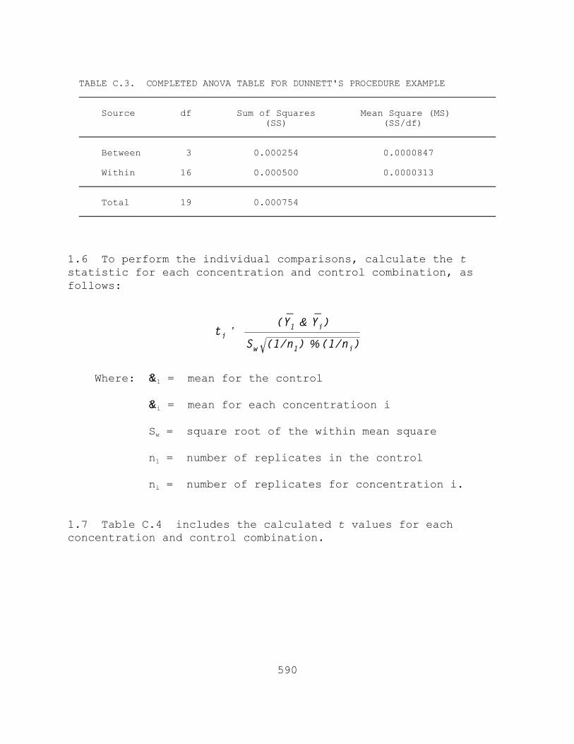
590

TABLE C.3. COMPLETED ANOVA TABLE FOR DUNNETT'S PROCEDURE EXAMPLE Source df Sum of Squares Mean Square (MS) (SS) (SS/df) Between 3 0.000254 0.0000847 Within 16 0.000500 0.0000313 Total 19 0.000754

ti '(Y1 & Yi)

Sw (1/n1) % (1/ni)

1.6 To perform the individual comparisons, calculate the tstatistic for each concentration and control combination, asfollows:

Where: &Y1 = mean for the control

&Yi = mean for each concentratioon i Sw = square root of the within mean square n1 = number of replicates in the control ni = number of replicates for concentration i.

1.7 Table C.4 includes the calculated t values for eachconcentration and control combination.

591

TABLE C.4. CALCULATED t VALUES )))))))))))))))))))))))))))))))))))))))))))))))))))))))))))))))))))))))))) Concentration (ppb) i ti )))))))))))))))))))))))))))))))))))))))))))))))))))))))))))))))))))))))))) 1.80 2 1.131 3.20 3 1.131 5.60 4 3.111))))))))))))))))))))))))))))))))))))))))))))))))))))))))))))))))))))))))))

1.8 Since the purpose of the test is only to detect a decreasein growth from the control, a one-sided test is appropriate. Thecritical value for the one-sided comparison is read from thetable of Dunnett's "t" values (Table C.5; this table assumes anequal number of replicates in all treatment concentrations andthe control). For this set of data, with an overall alpha levelof 0.05, 16 degrees of freedom and three concentrations excludingthe control, the critical value is 2.23. The mean weight forconcentration "i" is considered significantly less than the meanweight for the control if ti is greater than the critical value. Comparing each of the calculated t values in Table C.4 with thecritical value, a significant decrease in growth from the controlis detected in the 5.60% concentration. Therefore, the NOEC andthe LOEC for growth are 3.20% and 5.60%, respectively.

592

TABL

E C.

5.

DUNN

ETT'

S "T

" VA

LUES

(Mill

er,

1981

) (O

ne-t

aile

d)dak

v

ka

= .0

5a

= 0.1

12

34

56

78

91

23

45

67

89

52.

022.

442.

682.

852.

983.

083.

163.

243.

303.

373.

904.

214.43

4.60

4.73

4.85

4.94

5.03

61.

942.

342.

562.

712.

832.

923.

003.

073.

123.

143.

613.

884.07

4.21

4.33

4.43

4.51

4.59

71.

892.

272.

482.

622.

732.

822.

892.

953.

013.

003.

423.

563.83

3.96

4.07

4.15

4.23

4.30

81.

862.

222.

422.

552.

662.

742.

812.

872.

922.

903.

293.

513.67

3.79

3.88

3.96

4.03

4.09

91.

832.

182.

372.

502.

602.

682.

752.

812.

862.

823.

193.

403.55

3.66

3.75

3.82

3.89

3.94

101.

812.

152.

342.

472.

562.

642.

702.

762.

812.

763.

113.

313.45

3.56

3.64

3.71

3.78

3.83

111.

802.

132.

312.

442.

532.

602.

672.

722.

772.

723.

063.

253.38

3.48

3.56

3.63

3.69

3.74

121.

782.

112.

292.

412.

502.

582.

642.

692.

742.

683.

013.

193.32

3.42

3.50

3.56

3.62

3.67

131.

772.

092.

272.

392.

482.

552.

612.

662.

712.

652.

973.

153.27

3.37

3.44

3.91

3.56

3.61

141.

762.

082.

252.

372.

462.

532.

592.

642.

692.

622.

943.

113.23

3.32

3.40

3.46

3.51

3.56

151.

752.

072.

242.

362.

442.

512.

572.

622.

672.

602.

913.

083.20

3.29

3.36

3.42

3.47

3.52

161.

752.

062.

232.

342.

432.

502.

562.

612.

652.

582.

883.

053.17

3.26

3.33

3.39

3.44

3.48

171.

742.

052.

222.

332.

422.

492.

542.

592.

642.

572.

863.

033.14

3.23

3.30

3.36

3.41

3.45

181.

732.

042.

212.

322.

412.

482.

532.

582.

622.

552.

843.

013.12

3.21

3.27

3.33

3.38

3.42

191.

732.

032.

202.

312.

402.

472.

522.

572.

612.

542.

832.

993.10

3.18

3.25

3.31

3.36

3.40

201.

722.

032.

192.

302.

392.

462.

512.

562.

602.

532.

812.

973.08

3.17

3.23

3.29

3.34

3.38

241.

712.

012.

172.

282.

362.

432.

482.

532.

572.

492.

772.

923.03

3.11

3.17

3.22

3.27

3.31

301.

701.

992.

152.

252.

332.

402.

452.

502.

542.

462.

722.

872.97

3.05

3.11

3.16

3.21

3.24

401.

681.

972.

132.

232.

312.

372.

422.

472.

512.

422.

682.

822.92

2.99

3.05

3.10

3.14

3.18

601.

671.

952.

102.

212.

282.

352.

392.

442.

482.

392.

642.

782.87

2.94

3.00

3.04

3.08

3.12

120

1.66

1.93

2.08

2.18

2.26

2.32

2.37

2.41

2.45

2.36

2.60

2.73

2.82

2.90

2.94

2.99

3.03

3.06

593

MSD'd Sw (1/n1)%(1/n)

MSD ' 2.23(0.00559) (1/5)%(1/5)

1.9 To quantify the sensitivity of the test, the minimumsignificant difference (MSD) may be calculated. The formula isas follows:

Where:d = critical value for the Dunnett's Procedure

Sw = the square root of the within mean square

n = the number of replicates at each concentration,assuming an equal number of replicates at alltreatment concentrations

n1 = number of replicates in the control

For example:

= 2.23 (0.00559)(0.632)

= 0.00788

1.10 Therefore, for this set of data, the minimum differencebetween the control mean and a concentration mean that can bedetected as statistically significant is 0.00788 mg. Thisrepresents a 15.2% reduction in mean weight from the control.

1.11 If the data have not been transformed, the MSD (and thepercent decrease from the control mean that it represents) can bereported as is.

1.11.1 In the case where the data have been transformed, the MSDwould be in transformed units. In this case carry out thefollowing conversion to determine the MSD in untransformed units.

1.11.2 Subtract the MSD from the transformed control mean. Callthis difference D. Next, obtain untransformed values for thecontrol mean and the difference, D. Finally, compute theuntransformed MSD as follows:

594

MSDu = controlu - Du

Where: MSDu = the minimum significant difference foruntransformed data Controlu = the untransformed control mean

Du = the untransformed difference 1.11.3 Calculate the percent reduction from the control thatMSDu represents as: MSDu Percent Reduction = )))))))))))) X 100 Controlu 1.11.3.1 An example of a conversion of the MSD to untransformedunits, when the arc sine square root transformation was used onthe data, follows.

Step 1. Subtract the MSD from the transformed control mean. As an example, assume the data in Table C.1 weretransformed by the arc sine square roottransformation. Thus:

0.052 - 0.00788 = 0.04412

Step 2. Obtain untransformed values for the control mean(0.052) and the difference (0.04412) obtained inStep 1, above.

[ Sine (0.052)]2 = 0.00270

[ Sine (0.04412)]2 = 0.00195

Step 3. The untransformed MSD (MSDu) is determined bysubtracting the untransformed values obtained inStep 2.

MSDu = 0.00270 - 0.00195 = 0.00075

In this case, the MSD would represent a 1.4% decrease in survivalfrom the control [(0.00075/0.052)(100)].

595

2. COMPUTER CALCULATIONS

2.1 This computer program incorporates two analyses: ananalysis of variance (ANOVA), and a multiple comparison oftreatment means with the control mean (Dunnett's Procedure). TheANOVA is used to obtain the error value. Dunnett's Procedureindicates which toxicant concentration means (if any) arestatistically different from the control mean at the 5% level ofsignificance. The program also provides the minimum differencebetween the control and treatment means that could be detected asstatistically significant, and tests the validity of thehomogeneity of variance assumption by Bartlett's Test. Themultiple comparison is performed based on procedures described byDunnett (1955).

2.2 The source code for the Dunnett's program is structured intoa series of subroutines, controlled by a driver routine. Eachsubroutine has a specific function in the Dunnett's Procedure,such as data input, transforming the data, testing for equalityof variances, computing p values, and calculating the one-wayanalysis of variance.

2.3 The program compares up to seven toxicant concentrationsagainst the control, and can accommodate up to 50 replicates perconcentration.

2.4 If the number of replicates at each toxicant concentrationand control are not equal, a t test with the Bonferroniadjustment is performed instead of Dunnett's Procedure (seeAppendix D).

2.5 The program was written in IBM-PC FORTRAN by ComputerSciences Corporation, 26 W. Martin Luther King Drive, Cincinnati,OH 45268. A compiled version of the program can be obtained fromEMSL-Cincinnati by sending a diskette with a written request.

2.6 DATA INPUT AND OUTPUT

2.6.1 The mysid growth data from Table C.1 are used toillustrate the data input and output for this program.

2.6.2 Data Input

596

2.6.2.1 When the program is entered, the user is asked to selectthe type of data to be analyzed:

1. Response proportions, like survival or fertilizationproportions data.

2. Counts and measurements, like offspring counts, cystocarpand algal cell counts, weights, chlorophyll measurementsor turbidity measurements.

2.6.2.2 After the type of analysis for the data is chosen, theuser has the following options:

1. Create a data file 2. Edit a data file 3. Perform analysis on existing data set 4. Stop

2.6.2.3 When Option 1 (Create a data file) is selected forresponse proportions, the program prompts the user for thefollowing information:

1. Number of concentrations, including control2. For each concentration and replicate:

- number of organisms exposed per replicate - number of organisms responding per replicate (organisms surviving, eggs fertilized, etc.)

2.6.2.4 After the data have been entered, the user may save thefile on a disk, and the program returns to the main menu (seebelow).

2.6.2.5 Sample data input is shown in Figure C.1.

2.6.3. Program Output

2.6.3.1 When Option 3 (perform analysis on existing data set) isselected from the menu, the user is asked to select thetransformation desired, and indicate whether they expect themeans of the test groups to be less or greater than the mean forthe control group (see Figure C.2).

597

EMSL Cincinnati Dunnett Software Version 1.5

What type of data do you wish to analyze?

1) response proportions (like survival data or fertility proportion data) Note: The program calculates a proportion after prompting for number of exposed organisms and number of responding organisms.

2) counts and measurements (like offspring counts, cystocarps and algal cell counts, weights, chlorophyll measurements, or turbidity measurements)

Enter "1", "2", (or "q" to quit program): 2

Title ? Appendix C, Dunnett's Procedure Example - Mysid Data

Output to printer or disk file ? P

1) Create a data file 2) Edit a data file 3) Analyze an existing data set 4) Stop

Your choice ? 1

Number of concentrations, including control ? 4

Number of observations for conc. 1 (the control) ? 5

Enter the data for conc. 1 (the control) one observation at a time.

NO. 1? 0.048

NO. 2? 0.058

NO. 3? 0.047

NO. 4? 0.058

NO. 5? 0.051

Figure C.1. Sample Data Input for Dunnett's Program for Survival Data fromTable C.1.

598

Enter the data for conc. 2 one observation at a time.

NO. 1? 0.055

NO. 2? 0.048

NO. 3? 0.042

NO. 4? 0.041

NO. 5? 0.052

Number of observations for conc. 3 ? 5

Enter the data for conc. 3 one observation at a time.

NO. 1? 0.057

NO. 2? 0.050

NO. 3? 0.046

NO. 4? 0.043

NO. 5? 0.045

Number of observations for conc. 4 ? 5

Enter the data for conc. 4 one observation at a time.

NO. 1? 0.041

NO. 2? 0.040

NO. 3? 0.041

NO. 4? 0.043

NO. 5? 0.040

Do you wish to save the data on disk ? Y

Disk file for output ? c:\mysid.dat

Figure C.1. Sample Data Input for Dunnett's Program for Survival Data fromTable C.1. (Continued)

599

EMSL Cincinnati Dunnett Software Version 1.5

1) Create a data file 2) Edit a data file 3) Analyze an existing data set 4) Stop

Your choice ? 3

File name ? c:\mysid.dat

Available Transformations 1) no transform 2) square root 3) log10

Your choice ? 1

Dunnett's test as implemented in this program is a one-sided test. You must specify the direction the test is to be run; that is, do you expect the means for the test concentrations to be less than or greater than the mean for the control concentration.

Direction for Dunnetts test : L=less than, G=greater than ? L

Figure C.2. Example of Choosing Option 3 from the Main Menu of the DunnettProgram.

600

2.6.3.2 Summary statistics (Figure C.3) for the raw andtransformed data, if applicable, the ANOVA table, results ofBartlett's Test, the results of the multiple comparisonprocedure, and the minimum detectable difference are included in the program output.

601

EMSL Cincinnati Dunnett Software Version 1.5

Appendix C, Dunnett's Procedure Example - Mysid Data

Summary Statistics and ANOVA

Transformation = None

Conc. n Mean s.d. cv%____________________________________________________________1 = control 5 .0524 .0053 10.2 2 5 .0476 .0061 12.8 3 5 .0482 .0055 11.5 4* 5 .0410 .0012 3.0____________________________________________________________

*) the mean for this conc. is significantly less than the control mean at alpha = 0.05 (1-sided) by Dunnett's test

Minimum detectable difference for Dunnett's test = -.006974This difference corresponds to -13.31 percent of control

Between concentrationssum of squares = .000333 with 3 degrees of freedom.

Error mean square = .000024 with 16 degrees of freedom.

Bartlett's test p-value for equality of variances = .060

Do you wish to restart the program ?

Figure C.3. Example of Program Output for the Dunnett's Program Using the Datain Table C.1.

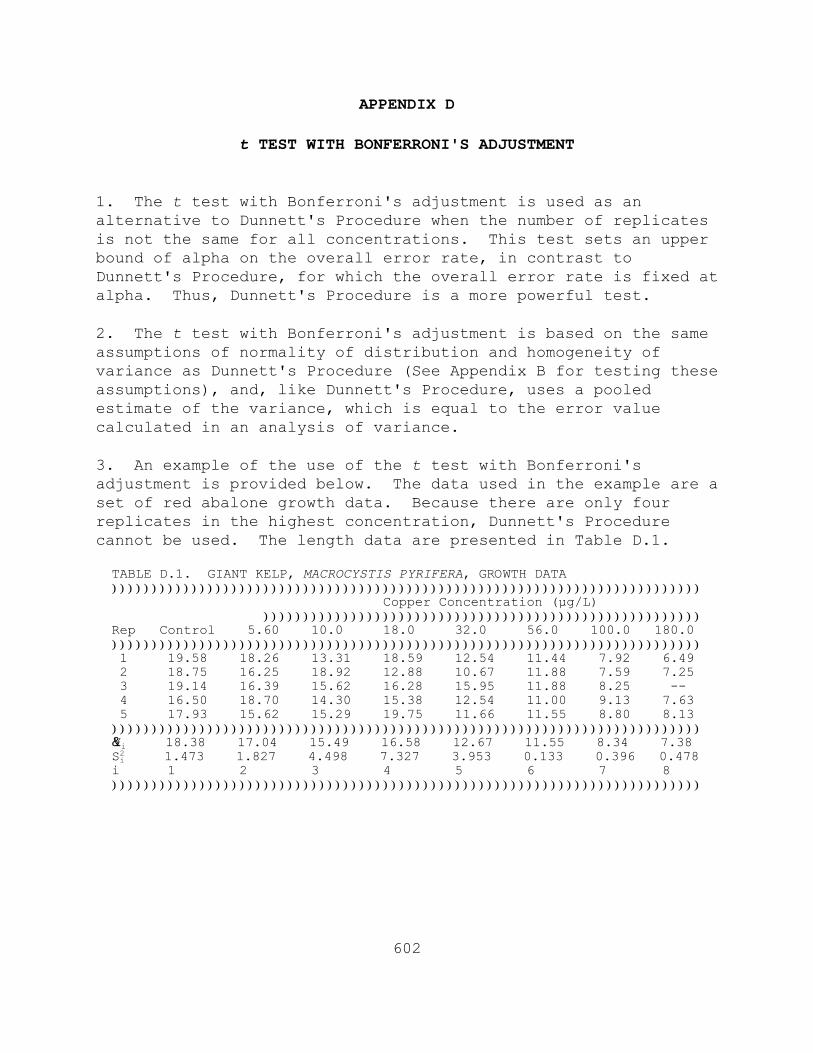
602

TABLE D.1. GIANT KELP, MACROCYSTIS PYRIFERA, GROWTH DATA)))))))))))))))))))))))))))))))))))))))))))))))))))))))))))))))))))))))))) Copper Concentration (µg/L) )))))))))))))))))))))))))))))))))))))))))))))))))))))))Rep Control 5.60 10.0 18.0 32.0 56.0 100.0 180.0)))))))))))))))))))))))))))))))))))))))))))))))))))))))))))))))))))))))))) 1 19.58 18.26 13.31 18.59 12.54 11.44 7.92 6.49 2 18.75 16.25 18.92 12.88 10.67 11.88 7.59 7.25 3 19.14 16.39 15.62 16.28 15.95 11.88 8.25 -- 4 16.50 18.70 14.30 15.38 12.54 11.00 9.13 7.63 5 17.93 15.62 15.29 19.75 11.66 11.55 8.80 8.13))))))))))))))))))))))))))))))))))))))))))))))))))))))))))))))))))))))))))Y&i 18.38 17.04 15.49 16.58 12.67 11.55 8.34 7.38Si2 1.473 1.827 4.498 7.327 3.953 0.133 0.396 0.478

i 1 2 3 4 5 6 7 8))))))))))))))))))))))))))))))))))))))))))))))))))))))))))))))))))))))))))

APPENDIX D

t TEST WITH BONFERRONI'S ADJUSTMENT

1. The t test with Bonferroni's adjustment is used as analternative to Dunnett's Procedure when the number of replicatesis not the same for all concentrations. This test sets an upperbound of alpha on the overall error rate, in contrast toDunnett's Procedure, for which the overall error rate is fixed atalpha. Thus, Dunnett's Procedure is a more powerful test.

2. The t test with Bonferroni's adjustment is based on the sameassumptions of normality of distribution and homogeneity ofvariance as Dunnett's Procedure (See Appendix B for testing theseassumptions), and, like Dunnett's Procedure, uses a pooledestimate of the variance, which is equal to the error valuecalculated in an analysis of variance.

3. An example of the use of the t test with Bonferroni'sadjustment is provided below. The data used in the example are aset of red abalone growth data. Because there are only fourreplicates in the highest concentration, Dunnett's Procedurecannot be used. The length data are presented in Table D.1.

603

TABLE D.2. ANOVA TABLE Source df Sum of Squares Mean Square(MS) (SS) (SS/df) 2 Between p - 1 SSB SB = SSB/(p-1) 2 Within N - p SSW SW = SSW/(N-p)

3.1 One way to obtain an estimate of the pooled variance is toconstruct an ANOVA table including all sums of squares, asdescribed in Table D.2:

Where: p = number of effluent concentrations includingthe control

N = the total sample size; N''ini

ni = the number of replicates for concentration i

SST''ijYij

2&G 2/N

Total Sum of Squares

Between Sum of SquaresSSB''iTi

2/ni&G2/N

Within Sum of SquaresSSW'SST&SSB

Where: G = The grand total of all sample

observations; G' 'Pi'1Ti

604

Ti = The total of the replicatemeasurements for concentration i

Yij = The jth observation for

concentration i 3.2 For the data in this example:

n1 = n2 = n3 = n4 = n5 = n6 = n7 = 5; n8 = 4

N = 39

T1 = Y11 + Y12 + Y13 + Y14 + Y15 = 91.90 T2 = Y21 + Y22 + Y23 + Y24 + Y25 = 85.22 T3 = Y31 + Y32 + Y33 + Y34 + Y35 = 77.44 T4 = Y41 + Y42 + Y43 + Y44 + Y45 = 82.88 T5 = Y51 + Y52 + Y53 + Y54 + Y55 = 63.36 T6 = Y61 + Y62 + Y63 + Y64 + Y65 = 57.75 T7 = Y71 + Y72 + Y73 + Y74 + Y75 = 41.69 T8 = Y81 + Y82 + Y83 + Y84 = 29.50

G = T1 + T2 + T3 + T4 + T5 + T6 + T7 + T8 = 529.74

SSB ' 'Pi'1

T 2i/ni&G

2/N

= 7749.905 - (529.74)2 = 554.406 39

SST ' 'Pi'1

'ni

j'1Y 2ij&G

2/N

= 7829.764 - (529.74)2 = 634.265 39

= 634.265 - 554.406 = 79.859 SSW ' SST&SSB

SB2 = SSB/(p-1) = 554.406/(8-1) = 79.201

SW2 = SSW/(N-p) = 79.859/(39-8) = 2.576

605

TABLE D.3. COMPLETED ANOVA TABLE FOR THE t TEST WITH BONFERRONI'SADJUSTMENT EXAMPLE

)))))))))))))))))))))))))))))))))))))))))))))))))))))))))))))))))))))))))) Source df Sum of Squares Mean Square (MS) (SS) (SS/df) )))))))))))))))))))))))))))))))))))))))))))))))))))))))))))))))))))))))))) Between 7 554.406 79.201 Within 31 79.859 2.576 )))))))))))))))))))))))))))))))))))))))))))))))))))))))))))))))))))))))))) Total 38 634.265 ))))))))))))))))))))))))))))))))))))))))))))))))))))))))))))))))))))))))))

ti '(Y1 & Yi)

Sw (1/n1) % (1/ni)

3.3 Summarize these calculations in the ANOVA table (Table D.3):

3.4 To perform the individual comparisons, calculate the tstatistic for each concentration and control combination, asfollows:

Where: &Yi = mean for concentration i

&Y1 = mean for the control

Sw = square root of the within mean square

n1 = number of replicates in the control.

ni = number of replicates for concentration i.

3.5 Table D.4 includes the calculated t values for eachconcentration and control combination.

606

TABLE D.4. CALCULATED t VALUES )))))))))))))))))))))))))))))))))))))))))))))))))))))))))))))))))))))))))) Concentration (µg/L) i ti )))))))))))))))))))))))))))))))))))))))))))))))))))))))))))))))))))))))))) 5.6 2 1.320 10.0 3 2.847 18.0 4 1.773 32.0 5 5.625 56.0 6 6.728 100.0 7 9.891 180.0 8 10.217))))))))))))))))))))))))))))))))))))))))))))))))))))))))))))))))))))))))))

3.6 Since the purpose of this test is to detect a significantreduction in mean length, a one-sided test is appropriate. Thecritical value for this one-sided test is found in Table D.5. For an overall alpha level of 0.05, 31 degrees of freedom forerror and seven concentrations (excluding the control) theapproximate critical value is 2.597. The mean length forconcentration "i" is considered significantly less than the meanlength for the control if ti is greater than the critical value. Comparing each of the calculated t values in Table D.4 with thecritical value, the 10.0 µg/L, 32 µg/L, 56.0 µg/L, 100.0 µg/L,180.0 µg/L concentrations have significantly lower mean lengththan the control. Because the 10.0 µg/L concentration showssignigicantly lower mean length that the control while the higher18.0 µg/L concentration does not, these test results areconsidered to have an anomalous dose-response relationship and itis recommended that the test be repeated. If an NOEC and LOECmust be determined for this test, the lowest concentration withsignificant growth impairment versus the control is considered tothe LOEC for growth. Thus, for this test, the NOEC and LOECwould be 5.6 µg/L and 10.0 µg/L, respectively.

607

TABLE D.5. CRITICAL VALUES FOR "t" FOR THE t TEST WITH BONFERRONI'S ADJUSTMENT P = 0.05

CRITICAL LEVEL, ONE TAILED

d.f.

K = 1

K = 2

K = 3

K = 4

K = 5

K = 6

K = 7

K = 8

K = 9

K = 10

1

6.314

12.707

19.002

25.452

31.821

38.189

44.556

50.924

57.290

63.657

2

2.920

4.303

5.340

6.206

6.965

7.649

8.277

8.861

9.408

9.925

3

2.354

3.183

3.741

4.177

4.541

4.857

5.138

5.392

5.626

5.841

4

2.132

2.777

3.187

3.496

3.747

3.961

4.148

4.315

4.466

4.605

5

2.016

2.571

2.912

3.164

3.365

3.535

3.681

3.811

3.927

4.033

6

1.944

2.447

2.750

2.969

3.143

3.288

3.412

3.522

3.619

3.708

7

1.895

2.365

2.642

2.842

2.998

3.128

3.239

3.336

3.422

3.500

8

1.860

2.307

2.567

2.752

2.897

3.016

3.118

3.206

3.285

3.356

9

1.834

2.263

2.510

2.686

2.822

2.934

3.029

3.111

3.185

3.250

10

1.813

2.229

2.406

2.634

2.764

2.871

2.961

3.039

3.108

3.170

11

1.796

2.201

2.432

2.594

2.719

2.821

2.907

2.981

3.047

3.106

12

1.783

2.179

2.404

2.561

2.681

2.778

2.863

2.935

2.998

3.055

13

1.771

2.161

2.380

2.533

2.651

2.746

2.827

2.897

2.958

3.013

14

1.762

2.145

2.360

2.510

2.625

2.718

2.797

2.864

2.924

2.977

15

1.754

2.132

2.343

2.490

2.603

2.694

2.771

2.837

2.895

2.947

16

1.746

2.120

2.329

2.473

2.584

2.674

2.749

2.814

2.871

2.921

17

1.740

2.110

2.316

2.459

2.567

2.655

2.729

2.793

2.849

2.899

18

1.735

2.101

2.305

2.446

2.553

2.640

2.712

2.775

2.830

2.879

19

1.730

2.094

2.295

2.434

2.540

2.626

2.697

2.759

2.813

2.861

20

1.725

2.086

2.206

2.424

2.528

2.613

2.684

2.745

2.798

2.846

21

1.721

2.080

2.278

2.414

2.518

2.602

2.672

2.732

2.785

2.832

22

1.718

2.074

2.271

2.406

2.509

2.592

2.661

2.721

2.773

2.819

23

1.714

2.069

2.264

2.398

2.500

2.583

2.651

2.710

2.762

2.808

24

1.711

2.064

2.258

2.391

2.493

2.574

2.642

2.701

2.752

2.797

25

1.709

2.060

2.253

2.385

2.486

2.566

2.634

2.692

2.743

2.788

608

TABLE D.5. CRITICAL VALUES FOR "t" FOR THE t TEST WITH BONFERRONI'S ADJUSTMENT

P = 0.05 CRITICAL LEVEL, ONE TAILED (CONTINUED)

df K = 1 K = 2 K = 3 K = 4 K = 5 K = 6 K = 7 K = 8 K = 9 K = 10

29 1.700 2.046 2.235 2.364 2.463 2.541 2.607 2.664 2.713 2.757

30 1.698 2.043 2.231 2.360 2.458 2.536 2.602 2.658 2.707 2.750

31 1.696 2.040 2.228 2.356 2.453 2.531 2.597 2.652 2.701 2.745

32 1.694 2.037 2.224 2.352 2.449 2.527 2.592 2.647 2.696 2.739

33 1.693 2.035 2.221 2.349 2.445 2.523 2.587 2.643 2.691 2.734

34 1.691 2.033 2.219 2.346 2.442 2.519 2.583 2.638 2.686 2.729

35 1.690 2.031 2.216 2.342 2.438 2.515 2.579 2.634 2.682 2.724

36 1.689 2.029 2.213 2.340 2.435 2.512 2.575 2.630 2.678 2.720

37 1.688 2.027 2.211 2.337 2.432 2.508 2.572 2.626 2.674 2.716

38 1.686 2.025 2.209 2.334 2.429 2.505 2.568 2.623 2.670 2.712

39 1.685 2.023 2.207 2.332 2.426 2.502 2.565 2.619 2.667 2.708

40 1.684 2.022 2.205 2.329 2.424 2.499 2.562 2.616 2.663 2.705

50 1.676 2.009 2.189 2.311 2.404 2.478 2.539 2.592 2.638 2.678

60 1.671 2.001 2.179 2.300 2.391 2.463 2.324 2.576 2.621 2.661

70 1.667 1.995 2.171 2.291 2.381 2.453 2.513 2.564 2.609 2.648

80 1.665 1.991 2.166 2.285 2.374 2.446 2.505 2.556 2.600 2.639

90 1.662 1.987 2.162 2.280 2.369 2.440 2.499 2.549 2.593 2.632

100 1.661 1.984 2.158 2.276 2.365 2.435 2.494 2.544 2.588 2.626

110 1.659 1.982 2.156 2.273 2.361 2.432 2.490 2.540 2.583 2.622

120 1.658 1.980 2.153 2.270 2.358 2.429 2.487 2.536 2.580 2.618

Infinite 1.645 1.960 2.129 2.242 2.327 2.394 2.450 2.498 2.540 2.576

______________________________________________________________________________________________

d.f. = Degrees of freedom for MSE (Mean Square Error) from ANOVA.

K = Number of concentrations to be compared to the control.

609

APPENDIX E

STEEL'S MANY-ONE RANK TEST

1. Steel's Many-one Rank Test is a nonparametric test forcomparing treatments with a control. This test is an alternativeto Dunnett's Procedure, and may be applied to data when thenormality assumption has not been met. Steel's Test requiresequal variances across the treatments and the control, but it isthought to be fairly insensitive to deviations from thiscondition (Steel, 1959). The tables for Steel's Test require anequal number of replicates at each concentration. If this is notthe case, use Wilcoxon's Rank Sum Test, with Bonferroni'sadjustment (See Appendix F).

2. For an analysis using Steel's Test, for each control andconcentration combination, combine the data and arrange theobservations in order of size from smallest to largest. Assignthe ranks to the ordered observations (1 to the smallest, 2 tothe next smallest, etc.). If ties occur in the ranking, assignthe average rank to the observation. (Extensive ties wouldinvalidate this procedure). The sum of the ranks within eachconcentration is then calculated. To determine if the responsein a concentration is significantly less than the response in thecontrol, the rank sum for each concentration is compared to thesignificant values of rank sums given later in the section. Inthis table, k equals the number of treatments excluding thecontrol and n equals the number of replicates for eachconcentration and the control.

3. An example of the use of this test is provided below. Thetest employs embryo-larval development data from a bivalve 48-hour chronic test. The data are listed in Table E.1.

4. For each control and concentration combination, combine thedata and arrange the observations in order of size from smallestto largest. Assign the ranks (1, 2, 3, ..., 8) to the orderedobservations (1 to the smallest, 2 to the next smallest, etc.). If ties occur in the ranking, assign the average rank to eachtied observation.

5. An example of assigning ranks to the combined data for thecontrol and 0.13 µg/L copper concentration is given in Table E.2.

610

This ranking procedure is repeated for each control andconcentration combination. The complete set of rankings islisted in Table E.3. The ranks are then summed for each toxicantconcentration, as shown in Table E.4.

6. For this set of data, determine if the development in any ofthe effluent concentrations is significantly lower than thedevelopment of the control organisms. If this occurs, the ranksum at that concentration would be significantly lower than therank sum of the control. Thus, compare the rank sums for thedevelopment at each of the various effluent concentrations withsome "minimum" or critical rank sum, at or below which thesurvival would be considered to be significantly lower than thecontrol. At a probability level of 0.05, the critical rank sumin a test with five concentrations and four replicates perconcentration, is 10 (see Table F.4).

7. Since the rank sums for the 0.50 µg/L and 1.00 µg/Lconcentration levels are equal to the critical value, theproportions of normal development in those concentrations areconsidered significantly less than that in the control. Since noother rank sum is less than or equal to the critical value, noother concentration has a significantly lower proportion normalthan the control. Because the 0.50 µg/L concentration showssignigicantly lower normal development than the control while thehigher 2.00 µg/L concentration does not, these test results areconsidered to have an anomalous dose-response relationship and itis recommended that the test be repeated. If an NOEC and LOECmust be determined for this test, the lowest concentration withsignificant impairment versus the control is considered to theLOEC for growth. Thus, for this test, the NOEC and LOEC would be0.25 µg/L and 0.50 µg/L, respectively.

611

TABLE E.1. BIVALVE EMBRYO-LARVAL DEVELOPMENT DATAS))))))))))))))))))))))))))))))))))))))))))))))))))))))))))))))))))))))))) Copper Concentration (µg/L) Replicate Control 0.13 0.25 0.50 1.00 2.00S))))))))))))))))))))))))))))))))))))))))))))))))))))))))))))))))))))))))) A 1.00 0.96 0.92 0.91 0.88 1.00RAW B 0.96 0.97 0.95 0.93 0.83 0.67 C 1.00 1.00 0.90 0.88 0.88 0.75 D 0.97 0.96 0.96 0.93 0.82 0.60S)))))))))))))))))))))))))))))))))))))))))))))))))))))))))))))))))))))))))ARC SINE A 1.571 1.369 1.284 1.266 1.217 1.571SQUARE ROOT B 1.369 1.397 1.345 1.303 1.146 0.959TRANSFORMED C 1.571 1.571 1.249 1.217 1.217 1.047 D 1.397 1.369 1.369 1.303 1.133 0.886S)))))))))))))))))))))))))))))))))))))))))))))))))))))))))))))))))))))))))Mean (Y&i) 1.477 1.427 1.312 1.272 1.178 1.116Si2 0.01191 0.00945 0.00303 0.00166 0.00203 0.09644i 1 2 3 4 5 6S)))))))))))))))))))))))))))))))))))))))))))))))))))))))))))))))))))))))))

612

TABLE E.2. ASSIGNING RANKS TO THE CONTROL AND 0.13 µg/L CONCENTRATIONLEVEL FOR STEEL'S MANY-ONE RANK TEST

)))))))))))))))))))))))))))))))))))))))))))))))))))))))))))))))))) Transformed Proportion

Rank Normal Concentration )))))))))))))))))))))))))))))))))))))))))))))))))))))))))))))))))) 2 1.369 0.13 µg/L 2 1.369 0.13 µg/L 2 1.369 Control 4.5 1.397 0.13 µg/L 4.5 1.397 Control 7 1.571 0.13 µg/L 7 1.571 Control 7 1.571 Control ))))))))))))))))))))))))))))))))))))))))))))))))))))))))))))))))))

613

TABLE E.3. TABLE OF RANKS1

)))))))))))))))))))))))))))))))))))))))))))))))))))))))))))))))))))))))))) Copper Concentration (µg/L) ))))))))))))))))))))))))))))))))Replicate Control 0.13 0.25))))))))))))))))))))))))))))))))))))))))))))))))))))))))))))))))))))))))))

1 1.571(7,7.5,7.5,7.5,7) 1.369(2) 1.284(2) 2 1.369(2,4.5,5,5,4) 1.397(4.5) 1.345(3) 3 1.571(7,7.5,7.5,7.5,7) 1.571(7) 1.249(1) 4 1.397(4.5,6,6,6,5) 1.369(2) 1.369(4.5)

-------------------------------------------------------------------------- Copper Concentration (µg/L) (Continued) ))))))))))))))))))))))))))))))))))))))))))))))))Replicate 0.50 1.00 2.00))))))))))))))))))))))))))))))))))))))))))))))))))))))))))))))))))))))))))

1 1.266(2) 1.217(3.5) 1.571(7) 2 1.303(3.5) 1.146(2) 0.959(2) 3 1.217(1) 1.217(3.5) 1.047(3) 4 1.303(3.5) 1.133(1) 0.886(1)

))))))))))))))))))))))))))))))))))))))))))))))))))))))))))))))))))))))))))1Control ranks are given in the order of the concentration with which they were ranked.

TABLE E.4. RANK SUMS ))))))))))))))))))))))))))))))))))))))))))))))))))))))))) Concentration µg/L Copper) Rank Sum ))))))))))))))))))))))))))))))))))))))))))))))))))))))))) 0.13 15.5 0.25 10.5 0.50 10.0 1.00 10.0 2.00 13.0 )))))))))))))))))))))))))))))))))))))))))))))))))))))))))

614

TABLE E.5. SIGNIFICANT VALUES OF RANK SUMS: JOINT CONFIDENCE COEFFICIENTS OF 0.95 (UPPER) and 0.99 (LOWER) FOR ONE-SIDED ALTERNATIVES (Steel, 1959) k = number of treatments (excluding control) % n % 2 3 4 5 6 7 8 9 % % 4 % 11 10 10 10 10 -- -- -- % -- -- -- -- -- -- -- -- 5 % 18 17 17 16 16 16 16 15 % 15 -- -- -- -- -- -- -- 6 % 27 26 25 25 24 24 24 23 % 23 22 21 21 -- -- -- -- 7 % 37 36 35 35 34 34 33 33 % 32 31 30 30 29 29 29 29 8 % 49 48 47 46 46 45 45 44 % 43 42 41 40 40 40 39 39 9 % 63 62 61 60 59 59 58 58 % 56 55 54 53 52 52 51 51 10 % 79 77 76 75 74 74 73 72 % 71 69 68 67 66 66 65 65 11 % 97 95 93 92 91 90 90 89 % 87 85 84 83 82 81 81 80 12 % 116 114 112 111 110 109 108 108 % 105 103 102 100 99 99 98 98 13 % 138 135 133 132 130 129 129 128 % 125 123 121 120 119 118 117 117 14 % 161 158 155 154 153 152 151 150 % 147 144 142 141 140 139 138 137 15 % 186 182 180 178 177 176 175 174 % 170 167 165 164 162 161 160 160 16 % 213 209 206 204 203 201 200 199 % 196 192 190 188 187 186 185 184 17 % 241 237 234 232 231 229 228 227 % 223 219 217 215 213 212 211 210 18 % 272 267 264 262 260 259 257 256 % 252 248 245 243 241 240 239 238 19 % 304 299 296 294 292 290 288 287 % 282 278 275 273 271 270 268 267 20 % 339 333 330 327 325 323 322 320 % 315 310 307 305 303 301 300 299

615

APPENDIX F

WILCOXON RANK SUM TEST

1. Wilcoxon's Rank Sum Test is a nonparametric test, to be usedas an alternative to Steel's Many-one Rank Test when the numberof replicates are not the same at each concentration. ABonferroni's adjustment of the pairwise error rate for comparisonof each concentration versus the control is used to set an upperbound of alpha on the overall error rate, in contrast to Steel'sMany-one Rank Test, for which the overall error rate is fixed atalpha. Thus, Steel's Test is a more powerful test.

2. The use of this test may be illustrated with devlopment datafrom the red abalone test in Table F.1. The control group hasfour replicates while each of the concentration levels has fivereplicates. Since there is 100% abnormality in all replicatesfor the 5.6% and 10.0% concentrations, they are not included inthe statistical analysis and are considered qualitativeabnormality effects.

3. For each concentration and control combination, combine thedata and arrange the values in order of size, from smallest tolargest. Assign ranks to the ordered observations (a rank of 1to the smallest, 2 to the next smallest, etc.). If ties in rankoccur, assign the average rank to each tied observation.

4. An example of assigning ranks to the combined data for thecontrol and effluent concentration 0.56% is given in Table F.2. This ranking procedure is repeated for each of the threeremaining control versus test concentration combinations. Thecomplete set of ranks is listed in Table F.3. The ranks are thensummed for each effluent concentration, as shown in Table F.4.

5. For this set of data, determine if the development in any ofthe test concentrations is significantly lower than thedevelopment in the control. If this occurs, the rank sum at thatconcentration would be significantly lower than the rank sum ofthe control. Thus, compare the rank sums for fecundity of eachof the various effluent concentrations with some "minimum" orcritical rank sum, at or below which the fecundity would beconsidered to be significantly lower than the control. At a

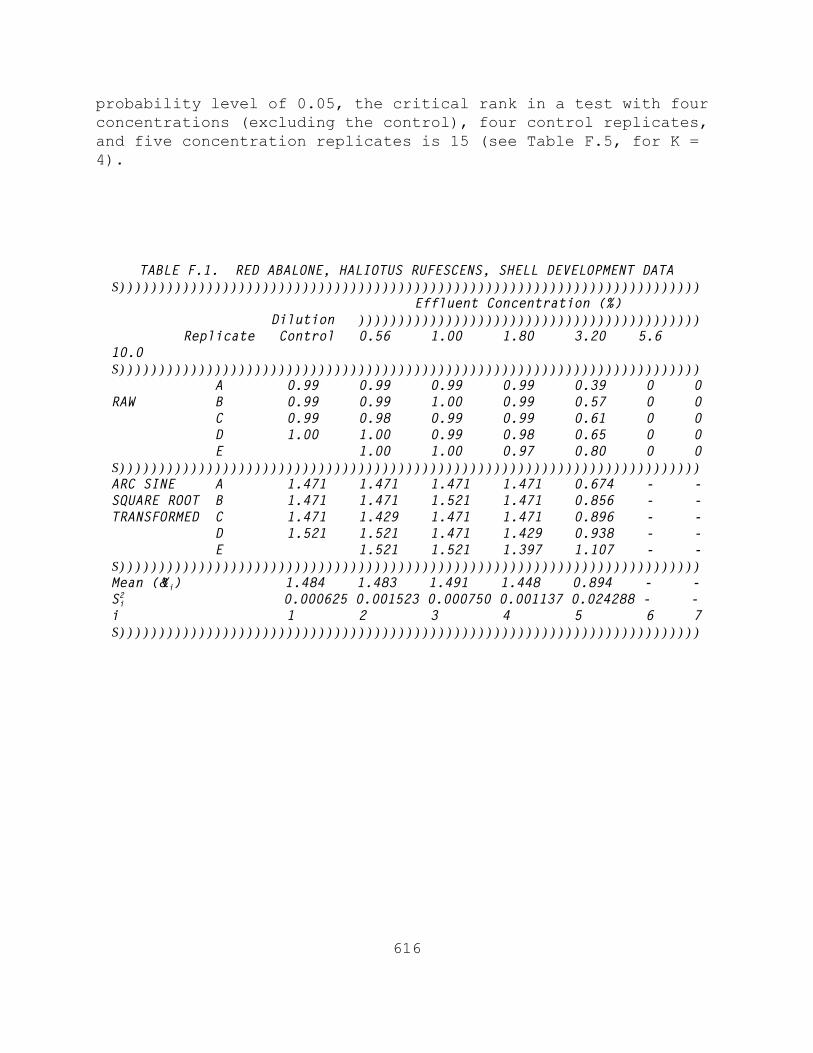
616

TABLE F.1. RED ABALONE, HALIOTUS RUFESCENS, SHELL DEVELOPMENT DATAS))))))))))))))))))))))))))))))))))))))))))))))))))))))))))))))))))))))))) Effluent Concentration (%) Dilution ))))))))))))))))))))))))))))))))))))))))))) Replicate Control 0.56 1.00 1.80 3.20 5.6 10.0S))))))))))))))))))))))))))))))))))))))))))))))))))))))))))))))))))))))))) A 0.99 0.99 0.99 0.99 0.39 0 0RAW B 0.99 0.99 1.00 0.99 0.57 0 0 C 0.99 0.98 0.99 0.99 0.61 0 0 D 1.00 1.00 0.99 0.98 0.65 0 0 E 1.00 1.00 0.97 0.80 0 0S)))))))))))))))))))))))))))))))))))))))))))))))))))))))))))))))))))))))))ARC SINE A 1.471 1.471 1.471 1.471 0.674 - -SQUARE ROOT B 1.471 1.471 1.521 1.471 0.856 - -TRANSFORMED C 1.471 1.429 1.471 1.471 0.896 - - D 1.521 1.521 1.471 1.429 0.938 - - E 1.521 1.521 1.397 1.107 - -S)))))))))))))))))))))))))))))))))))))))))))))))))))))))))))))))))))))))))Mean (Y&i) 1.484 1.483 1.491 1.448 0.894 - -Si2 0.000625 0.001523 0.000750 0.001137 0.024288 - -i 1 2 3 4 5 6 7S)))))))))))))))))))))))))))))))))))))))))))))))))))))))))))))))))))))))))

probability level of 0.05, the critical rank in a test with fourconcentrations (excluding the control), four control replicates,and five concentration replicates is 15 (see Table F.5, for K =4).

617

TABLE F.2. ASSIGNING RANKS TO THE CONTROL AND 0.56% CONCENTRATION LEVEL FOR THE WILCOXON RANK SUM TEST WITH THE BONFERRONI ADJUSTMENT

)))))))))))))))))))))))))))))))))))))))))))))))))))))))))))))))))) Transformed Proportion

Rank Normal Concentration )))))))))))))))))))))))))))))))))))))))))))))))))))))))))))))))))) 1 1.429 0.56 % 4 1.471 0.56 % 4 1.471 0.56 % 4 1.471 Control 4 1.471 Control 4 1.471 Control 8 1.521 0.56 % 8 1.521 0.56 % 8 1.521 Control ))))))))))))))))))))))))))))))))))))))))))))))))))))))))))))))))))

TABLE F.3. TABLE OF RANKS1

)))))))))))))))))))))))))))))))))))))))))))))))))))))))))))))))))))))))))) Effluent Concentration (%)Repli- )))))))))))))))))))))))))))))))))))))))))))))) cate Control 0.56 1.00 1.80 3.20))))))))))))))))))))))))))))))))))))))))))))))))))))))))))))))))))))))))))

1 1.471(4,3.5,5.5,7) 1.471(4) 1.471(3.5) 1.471(5.5) 0.674(1) 2 1.471(4,3.5,5.5,7) 1.471(4) 1.521(8) 1.471(5.5) 0.856(2) 3 1.471(4,3.5,5.5,7) 1.429(1) 1.471(3.5) 1.471(5.5) 0.896(3) 4 1.521(8,8,9,9) 1.521(8) 1.471(3.5) 1.429(2) 0.938(4) 5 1.521(8) 1.521(8) 1.397(1) 1.107(5)

))))))))))))))))))))))))))))))))))))))))))))))))))))))))))))))))))))))))))1Control ranks are given in the order of the concentration with which they were ranked.

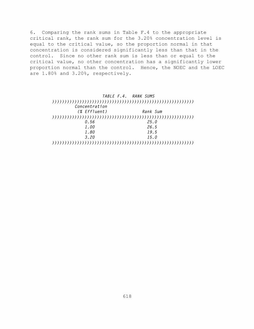
618

TABLE F.4. RANK SUMS ))))))))))))))))))))))))))))))))))))))))))))))))))))))))) Concentration (% Effluent) Rank Sum ))))))))))))))))))))))))))))))))))))))))))))))))))))))))) 0.56 25.0 1.00 26.5 1.80 19.5 3.20 15.0 )))))))))))))))))))))))))))))))))))))))))))))))))))))))))

6. Comparing the rank sums in Table F.4 to the appropriatecritical rank, the rank sum for the 3.20% concentration level isequal to the critical value, so the proportion normal in thatconcentration is considered significantly less than that in thecontrol. Since no other rank sum is less than or equal to thecritical value, no other concentration has a significantly lowerproportion normal than the control. Hence, the NOEC and the LOECare 1.80% and 3.20%, respectively.

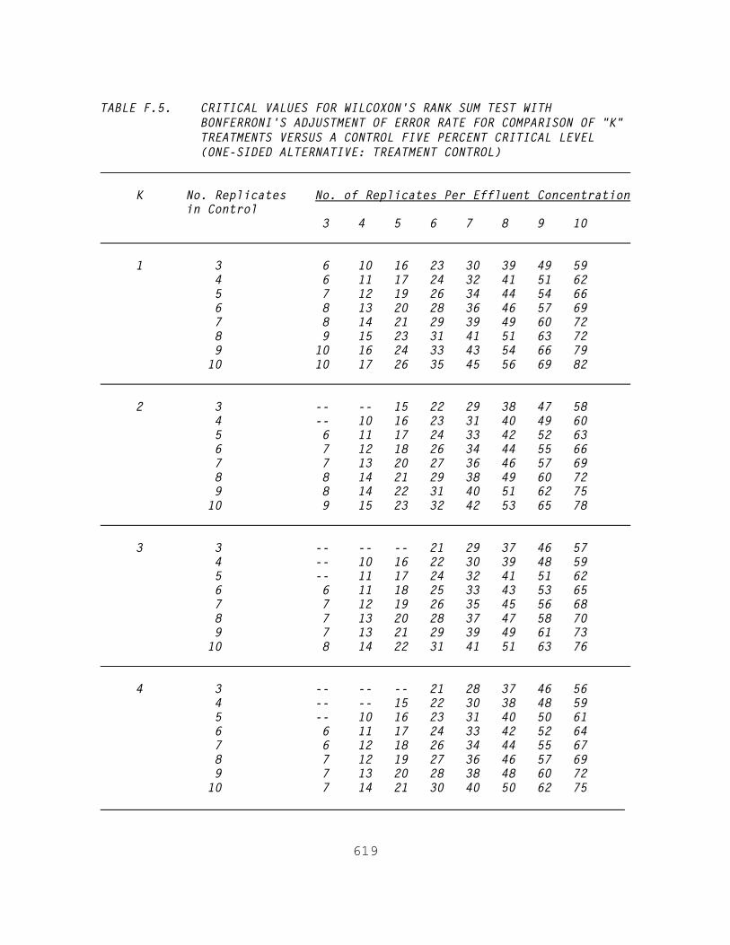
619

TABLE F.5. CRITICAL VALUES FOR WILCOXON'S RANK SUM TEST WITHBONFERRONI'S ADJUSTMENT OF ERROR RATE FOR COMPARISON OF "K"TREATMENTS VERSUS A CONTROL FIVE PERCENT CRITICAL LEVEL(ONE-SIDED ALTERNATIVE: TREATMENT CONTROL)

K No. Replicates No. of Replicates Per Effluent Concentration in Control 3 4 5 6 7 8 9 10 1 3 6 10 16 23 30 39 49 59 4 6 11 17 24 32 41 51 62 5 7 12 19 26 34 44 54 66 6 8 13 20 28 36 46 57 69 7 8 14 21 29 39 49 60 72 8 9 15 23 31 41 51 63 72 9 10 16 24 33 43 54 66 79 10 10 17 26 35 45 56 69 82 2 3 -- -- 15 22 29 38 47 58 4 -- 10 16 23 31 40 49 60 5 6 11 17 24 33 42 52 63 6 7 12 18 26 34 44 55 66 7 7 13 20 27 36 46 57 69 8 8 14 21 29 38 49 60 72 9 8 14 22 31 40 51 62 75 10 9 15 23 32 42 53 65 78

3 3 -- -- -- 21 29 37 46 57 4 -- 10 16 22 30 39 48 59 5 -- 11 17 24 32 41 51 62 6 6 11 18 25 33 43 53 65 7 7 12 19 26 35 45 56 68 8 7 13 20 28 37 47 58 70 9 7 13 21 29 39 49 61 73 10 8 14 22 31 41 51 63 76

4 3 -- -- -- 21 28 37 46 56 4 -- -- 15 22 30 38 48 59 5 -- 10 16 23 31 40 50 61 6 6 11 17 24 33 42 52 64 7 6 12 18 26 34 44 55 67 8 7 12 19 27 36 46 57 69 9 7 13 20 28 38 48 60 72 10 7 14 21 30 40 50 62 75

620

TABLE F.5. CRITICAL VALUES FOR WILCOXON'S RANK SUM TEST WITH BONFERRONI'SADJUSTMENT OF ERROR RATE FOR COMPARISON OF "K" TREATMENTSVERSUS A CONTROL FIVE PERCENT CRITICAL LEVEL (ONE-SIDEDALTERNATIVE: TREATMENT CONTROL) (CONTINUED)

K No. Replicates No. of Replicates Per Effluent Concentration in Control 3 4 5 6 7 8 9 10

5 3 -- -- -- -- 28 36 46 56 4 -- -- 15 22 29 38 48 58 5 -- 10 16 23 31 40 50 61 6 -- 11 17 24 32 42 52 63 7 6 11 18 25 34 43 54 66 8 6 12 19 27 35 45 56 68 9 7 13 20 28 37 47 59 71 10 7 13 21 29 39 49 61 74

6 3 -- -- -- -- 28 36 45 56 4 -- -- 15 21 29 38 47 58 5 -- 10 16 22 30 39 49 60 6 -- 11 16 24 32 41 51 63 7 6 11 17 25 33 43 54 65 8 6 12 18 26 35 45 56 68 9 6 12 19 27 37 47 58 70 10 7 13 20 29 38 49 60 73

7 3 -- -- -- -- -- 36 45 56 4 -- -- -- 21 29 37 47 58 5 -- -- 15 22 30 39 49 60 6 -- 10 16 23 32 41 51 62 7 -- 11 17 25 33 43 53 65 8 6 11 18 26 35 44 55 67 9 6 12 19 27 36 46 58 70 10 7 13 20 28 38 48 60 72

8 3 -- -- -- -- -- 36 45 55 4 -- -- -- 21 29 37 47 57 5 -- -- 15 22 30 39 49 59 6 -- 10 16 23 31 40 51 62 7 -- 11 17 24 33 42 53 64 8 6 11 18 25 34 44 55 67 9 6 12 19 27 36 46 57 69 10 6 12 19 28 37 48 59 72

621

TABLE F.5. CRITICAL VALUES FOR WILCOXON'S RANK SUM TEST WITH BONFERRONI'SADJUSTMENT OF ERROR RATE FOR COMPARISON OF "K" TREATMENTSVERSUS A CONTROL FIVE PERCENT CRITICAL LEVEL (ONE-SIDEDALTERNATIVE: TREATMENT CONTROL) (CONTINUED)

K No. Replicates No. of Replicates Per Effluent Concentration in Control 3 4 5 6 7 8 9 10

9 3 -- -- -- -- -- -- 45 55 4 -- -- -- 21 28 37 46 57 5 -- -- 15 22 30 39 48 59 6 -- 10 16 23 31 40 50 62 7 -- 10 17 24 33 42 52 64 8 -- 11 18 25 34 44 55 66 9 6 11 18 26 35 46 57 69 10 6 12 19 28 37 47 59 71

10 3 -- -- -- -- -- -- 45 55 4 -- -- -- 21 28 37 46 57 5 -- -- 15 22 29 38 48 59 6 -- 10 16 23 31 40 50 61 7 -- 10 16 24 32 42 52 64 8 -- 11 17 25 34 43 54 66 9 6 11 18 26 35 45 56 68 10 6 12 19 27 37 47 58 71

622

F 'S 21

S 22

where S 21 > S 2

2

APPENDIX G

SINGLE CONCENTRATION TOXICITY TEST - COMPARISON OF CONTROLWITH 100% EFFLUENT OR RECEIVING WATER OR COMPARISON OF

DILUTION AND BRINE CONTROLS

1. To statistically compare a control with one concentration,such as 100% effluent or the instream waste concentration, a ttest is the recommended analysis. The t test is based on theassumptions that the observations are independent and normallydistributed and that the variances of the observations are equalbetween the two groups. 2. Shapiro-Wilk's test may be used to test the normalityassumption (See Appendix B for details). For the two samplecase, the datasets must be tested for normality separately. Ifeither set of data does not meet the normality assumption, thenonparametric test, Wilcoxon's Rank Sum Test, may be used toanalyze the data. An example of this test is given in AppendixF. Since a control and one concentration are being compared, theK = 1 section of Table F.5 contains the needed critical valuesfor one-sided tests. An additional reference, such as Snedecorand Cochran (1980) must be used to determine critical values fortwo-sided tests, such as comparing brine and dilution controls. 3. The F test for equality of variances is used to test thehomogeneity of variance assumption. When conducting the F test,the alternative hypothesis of interest is that the variances arenot equal. 4. To make the two-tailed F test at the 0.01 level ofsignificance, put the larger of the two variances in thenumerator of F.

5. Compare F with the 0.005 level of a tabled F value with n1 -1 and n2 - 1 degrees of freedom, where n1 and n2 are the number ofreplicates for each of the two groups.

623

TABLE G.1. MYSID, HOLMESIMYSIS COSTATA, GROWTH DATA FROM A SINGLE-CONCENTATION EFFLUENT TEST

)))))))))))))))))))))))))))))))))))))))))))))))))))))))))))))))))))))))))) Replicate Control Effluent)))))))))))))))))))))))))))))))))))))))))))))))))))))))))))))))))))))))))) RAW A 0.048 0.041 B 0.058 0.033 C 0.047 0.044 D 0.055 0.040 E 0.051 0.043))))))))))))))))))))))))))))))))))))))))))))))))))))))))))))))))))))))))))Mean (Y&i) 0.052 0.040Si2 0.0000217 0.0000187i 1 2 ))))))))))))))))))))))))))))))))))))))))))))))))))))))))))))))))))))))))))

F '0.00002170.0000187

' 1.160

6. A set of mysid growth data from a single-concentrationeffluent test will be used to illustrate the F test. The rawdata, mean and variance for the two controls are given in TableG.1. The data from each concentration meets the assumption ofnormality.

7. Since the variability of the control is greater than thevariability of the effluent concentration, S2 for the control isplaced in the numerator of the F statistic and S2 for theeffluent concentration control is placed in the denominator.

8. There are 5 replicates for the each groups, so the numeratorand denominator degrees of freedom, ni - 1, are both 4. For atwo-tailed test at the 0.01 level of significance, the critical Fvalue is obtained from a table of the F distribution (Snedecorand Cochran, 1980). The critical F value for this test is 23.16. Since 2.41 is not greater than 23.16, conclude that the variancesof the brine and dilution controls are homogeneous.

9. Equal Variance t Test.

624

9.1 To perform the t test, calculate the following teststatistic:

t 'Y1 & Y2

Sp1n1

%1n2

Where: &Y1 = mean for the control

&Y2 = mean for the effluent concentration

Sp '(n1 & 1)S

21 % (n2 & 1)S

22

n1 % n2 & 2

S12 = estimate of the variance for the control

S22 = estimate of the variance for the effluent

concentration

n1 = number of replicates for the control

n2 = number of replicates for the effluent concentration

9.2 Since we are concerned here with a decrease in response fromthe control, a one-tailed test is appropriate. Thus, we willcompare the calculated t with a critical t, where the critical tis at the 5% level of significance with n1 + n2 - 2 degrees offreedom. If the calculated t exceeds the critical t, the meanresponses are declared different.

9.3 When comparing brine and dilution controls, the concern isfor any difference between the two control groups, and atwo-tailed test is appropriate. In that case, the calculated twould be compared with a critical t, where the critical t is atwo-tailed value at the 5% level of significance with n1 + n2 - 2degrees of freedom. If the absolute value of the calculated texceeds the critical t, the mean responses are declareddifferent.

625

t '0.052 & 0.040

0.00449 15

%15

' 4.226

Sp '(5 & 1) 0.0000217 % (5 & 1) 0.0000187

5 % 5 & 2' 0.00449

t 'Y1 & Y2

S 21

n1%

S 22

n2

9.4 Using the data from Table G.1 to illustrate the t test, thecalculation of t is as follows:

Where:9.5 For a one-tailed test at the 0.05 level of significance and8 degrees of freedom, the appropriate critical t value is 1.860. Note: Table D.5 for K = 1 includes the critical t values forcomparing two groups in a one-tailed test. Since t = 4.226 isgreater than 1.860, conclude that the growth in the effluentconcentration is significantly less than the control groupgrowth.

9.6 Critical t values for two-tailed tests, such as those neededin comparing a brine control and a dilution control, can be foundin a table of the t distribution, such as the one in Snedecor andCochran, 1980. Note that the critical t for a two-tailed test isthe upper-tail value at the a/2 level of significance.

10. UNEQUAL VARIANCE t TEST.

10.1 If the F test for equality of variance fails, the t test isstill a valid test. However, the denominator of the t statisticis adjusted as follows:

Where: &Y1 = mean for the control

626

df )'(n1&1) (n2&1)

(n2&1) C2%(1&C)2(n1&1)

&Y2 = mean for the effluent concentration

S12 = estimate of the variance for the control

S22 = estimate of the variance for the effluent

concentration

n1 = number of replicates for the control

n2 = number of replicates for the effluent concentration 10.2 Additionally, the degrees of freedom for the test areadjusted using the following formula:

Where:

C '

S 21

n1

S 21

n1%S 22

n2

10.3 The modified degrees of freedom is usually not an integer. Common practice is to round down to the nearest integer. 10.4 The t test is then conducted as the equal variance t test. The calculated t is compared to the critical t at the 0.05significance level with the modified degrees of freedom. If thecalculated t exceeds the critical t, the mean responses are foundto be statistically different.

627

TABLE H.1. DATA FOR PROBIT ANALYSIS)))))))))))))))))))))))))))))))))))))))))))))))))))))))))))))))))))))))))) Concentration (%) )))))))))))))))))))))))))))))))))))))))))))) Control 1.80 3.20 5.60 10.0 18.0))))))))))))))))))))))))))))))))))))))))))))))))))))))))))))))))))))))))))No. Dead 1 0 3 9 24 25No. Exposed 25 25 25 25 25 25))))))))))))))))))))))))))))))))))))))))))))))))))))))))))))))))))))))))))

APPENDIX H

PROBIT ANALYSIS

1. This program calculates the EC1 and EC50 (or LC1 and LC50),and the associated 95% confidence intervals.

2. The program is written in IBM PC Basic for the IBM compatiblePC by Computer Sciences Corporation, 26 W. Martin Luther KingDrive, Cincinnati, OH 45268. A compiled, executable version ofthe program and supporting documentation can be obtained fromEMSL-Cincinnati by sending a written request to EMSL at 3411Church Street, Cincinnati, OH 45244.

2.1 A set of mortality data from a mysid survival and growthtest is given in Table H.1. The program's data input routine isillustrated with this data in Figure H.1. The program beginswith a request for the following information:

1. Desired output of abbreviated (A) or full (F) output? (Note: only abbreviated output is shown below.)

2. Output designation (P = printer, D = disk file). 3. Title for the output. 4. The number of exposure concentrations.5. Toxicant concentration data.2.2 The program output for

the abbreviated output options, shown in Figure H.2,includes the following:

2.2 The program output for the abbreviated output options, shownin figure H.2, includes the following:

628

1. A table of the observed proportion responding andthe proportion responding adjusted for thecontrols.

2. The calculated chi-square statistic forheterogeneity and the tabular value. This test isone indicator of how well the data fit the model. The program will issue a warning when the testindicates that the data do not fit the model.

3. The estimated LC1 and LC50 values and associated95% confidence intervals.

629

$$$$$$$$$$$$$$$$$$$$$$$$$$$$$$$$$$$$$$$$$$$$$$$$$$$$$$$$$$$$$ $ $ $ EPA PROBIT ANALYSIS PROGRAM $ $ USED FOR CALCULATING LC/EC VALUES $ $ Version 1.5 $ $$$$$$$$$$$$$$$$$$$$$$$$$$$$$$$$$$$$$$$$$$$$$$$$$$$$$$$$$$$$$

Do you wish abbreviated (A) or full (F) input/output? AOutput to printer (P) or disk file (D)? PTitle ? Example of Probit Analysis for Appendix H

Number responding in the control group = ? 1Number of animals exposed in the concurrent control group = ? 25Number of exposure concentrations, exclusive of controls ? 5

Input data starting with the lowest exposure concentration

Concentration = ? 1.80Number responding = ? 0Number exposed = ? 25

Concentration = ? 3.20Number responding = ? 3Number exposed = ? 25

Concentration = ? 5.60Number responding = ? 9Number exposed = ? 25

Concentration = ? 10.0Number responding = ? 24Number exposed = ? 25

Concentration = ? 18.0Number responding = ? 25Number exposed = ? 25

Number Number Number Conc. Resp. Exposed ______ ______ ______ _______ 1 1.8000 0 25 2 3.2000 3 25 3 5.6000 9 25 4 10.0000 24 25 5 18.0000 25 25

Do you wish to modify your data ? N

The number of control animals which responded = 1The number of control animals exposed = 25Do you wish to modify these values ? N

630

Example of Probit Analysis for Appendix H

Proportion Observed Responding Number Number Proportion Adjusted for Conc. Exposed Resp. Responding Controls Control 25 1 0.0400 0.0000 1.8000 25 0 0.0000 -.0306 3.2000 25 3 0.1200 0.0930 5.6000 25 9 0.3600 0.3404 10.0000 25 24 0.9600 0.9588 18.0000 25 25 1.0000 1.0000 Chi - Square for Heterogeneity (calculated) = 3.004Chi - Square for Heterogeneity (tabular value at 0.05 level) = 7.815 Example of Probit Analysis for Appendix H Estimated LC/EC Values and Confidence Limits Exposure 95% Confidence LimitsPoint Conc. Lower Upper LC/EC 1.00 2.642 1.384 3.519LC/EC 50.00 5.973 4.998 6.920

Figure H.2. USEPA Probit Analysis Program used for Calculating LC/ECValues, Version 1.5.

631

APPENDIX I

SPEARMAN-KARBER METHOD

1. The Spearman-Karber Method is a nonparametric statisticalprocedure for estimating the LC50 and the associated 95%confidence interval (Finney, 1978). The Spearman-Karber Methodestimates the mean of the distribution of the log10 of thetolerance. If the log tolerance distribution is symmetric, thisestimate of the mean is equivalent to an estimate of the medianof the log tolerance distribution.

2. If the response proportions are not monotonically non-decreasing with increasing concentration (constant or steadilyincreasing with concentration), the data must be smoothed. Abbott's procedure is used to "adjust" the concentration responseproportions for mortality occurring in the control replicates.

3. Use of the Spearman-Karber Method is recommended when partialmortalities occur in the test solutions, but the data do not fitthe Probit model.

4. To calculate the LC50 using the Spearman-Karber Method, thefollowing must be true: 1) the smoothed adjusted proportionmortality for the lowest effluent concentration (not includingthe control) must be zero, and 2) the smoothed adjustedproportion mortality for the highest effluent concentration mustbe one.

5. To calculate the 95% confidence interval for the LC50estimate, one or more of the smoothed adjusted proportionmortalities must be between zero and one.

6. The Spearman-Karber Method is illustrated below using a setof mortality data from a Mysid Survival and Growth test. Thesedata are listed in Table I.1.

632

TABLE I.1. EXAMPLE OF SPEARMAN-KARBER METHOD: MORTALITY DATA FROM A MYSID SURVIVAL AND GROWTH TEST (25 ORGANISMS PERCONCENTRATION)

S))))))))))))))))))))))))))))))))))))))))))))))))))))))))))))))))))Q Effluent Number of Mortality Concentration Mortalities Proportion % S))))))))))))))))))))))))))))))))))))))))))))))))))))))))))))))))))Q Control 2 0.08 6.25 2 0.08 12.5 0 0.00 25.0 3 0.12 50.0 16 0.64 100.0 25 1.00 S))))))))))))))))))))))))))))))))))))))))))))))))))))))))))))))))))Q

p si&1 ' p s

i ' (pi%pi&1)/2

p s0 ' p s

1 ' p s2 '

0.08%0.08%0.003

'0.163

' 0.053

7. Let p0, p1, ..., pk denote the observed response proportionmortalities for the control and k effluent concentrations. Thefirst step is to smooth the pi if they do not satisfy p0 # p1 #... # pk. The smoothing process replaces any adjacent pi's thatdo not conform to p0 # p1 # ... # pk with their average. Forexample, if pi is less than pi-1 then:

Where: pis = the smoothed observed proportionmortality for effluent concentration i.

7.1 For the data in this example, because the observed mortalityproportions for the control and the 6.25% effluent concentrationare greater than the observed response proportions for the 12.5%effluent concentration, the responses for these three groups mustbe averaged:

633

TABLE I.2. EXAMPLE OF SPEARMAN-KARBER METHOD: SMOOTHED, ADJUSTED MORTALITY DATA FROM A MYSID SURVIVAL AND GROWTH TEST

Smoothed, Effluent Smoothed Adjusted Concentration Mortality Mortality Mortality % Proportion Proportion Proportion

Control 0.08 0.053 0.000 6.25 0.08 0.053 0.000 12.5 0.00 0.053 0.000 25.0 0.12 0.120 0.071 50.0 0.64 0.640 0.620 100.0 1.00 1.000 1.000

p a0 ' p a

1 ' p a2 '

p s1 & p s

0

1 & p s0

'0.053 & 0.053

1 & 0.053'

0.00.947

' 0.0

7.2 Since p3 = 0.12 is larger than p2s, set p3s = 0.12. Similarly,p4 = 0.64 is larger than p3

s, so set p4s = 0.64. Finally, p5 = 1.00is larger than p4

s, so set p5s = 1.00. Additional smoothing is not

necessary. The smoothed observed proportion mortalities areshown in Table I.2.

8. Adjust the smoothed observed proportion mortality in eacheffluent concentration for mortality in the control group usingAbbott's formula (Finney, 1971). The adjustment takes the form:

pia = (pi

s - p0s) / (1 - p0s)

Where: p0s = the smoothed observed proportion mortality for the

control

pis = the smoothed observed proportion mortality for

effluent concentration i.

8.1 For the data in this example, the data for each effluentconcentration must be adjusted for control mortality usingAbbott's formula, as follows:

634

p a3 '

p s3 & p s

0

1 & p s0

'0.120 & 0.053

1 & 0.053'

0.0670.947

' 0.071

p a4 '

p s4 & p s

0

1 & p s0

'0.640 & 0.053

1 & 0.053'

0.5870.947

' 0.620

p a5 '

p s5 & p s

0

1 & p s0

'1.000 & 0.053

1 & 0.053'

0.9470.947

' 1.000

m ' 'k&1i'1

(p ai%1&p

ai )(Xi%Xi%1)

2

The smoothed, adjusted response proportions for the effluentconcentrations are shown in Table I.2. A plot of the smoothed,adjusted data is shown in Figure I.1.

9. Calculate the log10 of the estimated LC50, m, as follows:

Where: pia = the smoothed adjusted proportion mortality at

concentration i

Xi = the log10 of concentration i

k = the number of effluent concentrations tested, not including the control.

9.1 For this example, the log10 of the estimated LC50, m, iscalculated as follows:

m = [(0.000 - 0.000) (0.7959 + 1.0969)]/2 + [(0.071 - 0.000) (1.0969 + 1.3979)]/2 + [(0.620 - 0.071) (1.3979 + 1.6990)]/2 + [(1.000 - 0.620) (1.6990 + 2.0000)]/2

= 1.64147

635

Figure I.1

. P

lot

of o

bser

ved,

smo

othe

d, a

nd a

djus

ted

resp

onse

proportions for mysid,

Hol

mesi

mysi

s co

stat

a, s

urvi

val

data

.

636

V(m) ' 'k&1i'2

p ai (1&p

ai )(Xi%1&Xi&1)

2

4(ni&1)

1.64147 ± 2 0.0011388 ' (1.57398, 1.70896)

10. Calculate the estimated variance of m as follows:

Where: Xi = the log10 of concentration i

ni = the number of organisms tested at effluent concentration i

pi

a = the smoothed adjusted observed proportion mortality at effluent concentration i

k = the number of effluent concentrations tested, not including the control.

10.1 For this example, the estimated variance of m, V(m), iscalculated as follows:

V(m) = (0.000)(1.000)(1.3979 - 0.7959)2/4(24) + (0.071)(0.929)(1.6990 - 1.0969)2/4(24) + (0.620)(0.380)(2.0000 - 1.3979)2/4(24)

= 0.0011388

11. Calculate the 95% confidence interval for m:

m ± 2.0 V(m)

11.1 For this example, the 95% confidence interval for m iscalculated as follows:

12. The estimated LC50 and a 95% confidence interval for theestimated LC50 can be found by taking base10 antilogs of theabove values.

637

12.1 For this example, the estimated LC50 is calculated asfollows:

LC50 = antilog(m) = antilog(1.64147) = 43.8%.

12.2 The limits of the 95% confidence interval for the estimatedLC50 are calculated by taking the antilogs of the upper and lowerlimits of the 95% confidence interval for m as follows:

lower limit: antilog(1.57398) = 37.5%

upper limit: antilog(1.70896) = 51.2%

638

APPENDIX J

TRIMMED SPEARMAN-KARBER METHOD

1. The Trimmed Spearman-Karber Method is a modification of theSpearman-Karber Method, a nonparametric statistical procedure forestimating the LC50 and the associated 95% confidence interval(Hamilton, et al, 1977). The Trimmed Spearman-Karber Methodestimates the trimmed mean of the distribution of the log10 ofthe tolerance. If the log tolerance distribution is symmetric,this estimate of the trimmed mean is equivalent to an estimate ofthe median of the log tolerance distribution.

2. If the response proportions are not monotonically non-decreasing with increasing concentration (constant or steadilyincreasing with concentration), the data must be smoothed. Abbott's procedure is used to "adjust" the concentration responseproportions for mortality occurring in the control replicates.

3. Use of the Trimmed Spearman-Karber Method is recommended onlywhen the requirements for the Probit Analysis and the Spearman-Karber Method are not met.

4. To calculate the LC50 using the Trimmed Spearman-KarberMethod, the smoothed, adjusted, observed proportion mortalitiesmust bracket 0.5.

5. To calculate the 95% confidence interval for the LC50estimate, one or more of the smoothed, adjusted, observedproportion mortalities must be between zero and one.

6. Let p0, p1, ..., pk denote the observed proportion mortalitiesfor the control and the k effluent concentrations. The firststep is to smooth the pi if they do not satisfy p0 # p1 # ... #pk. The smoothing process replaces any adjacent pi's that do notconform to p0 # p1 # ... # pk, with their average. For example,if pi is less than pi-1 then:

pis-1 = pis = (pi + pi-1)/2

Where: pis = the smoothed observed proportion mortality foreffluent concentration i.

639

7. Adjust the smoothed observed proportion mortality in eacheffluent concentration for mortality in the control group usingAbbott's formula (Finney, 1971). The adjustment takes the form:

pia = (pis - p0

s) / (1 - p0s)

Where: p0s = the smoothed observed proportion mortality for the

control

pis = the smoothed observed proportion mortality for

effluent concentration i.

8. Calculate the amount of trim to use in the estimation of theLC50 as follows:

Trim = max(p1a, 1-pk

a)

Where: p1a = the smoothed, adjusted proportion mortality forthe lowest effluent concentration, exclusive ofthe control

pka = the smoothed, adjusted proportion mortality forthe highest effluent concentration

k = the number of effluent concentrations, exclusiveof the control.

The minimum trim should be calculated for each data set ratherthan using a fixed amount of trim for each data set.

9. Due to the intensive nature of the calculation for theestimated LC50 and the calculation of the associated 95%confidence interval using the Trimmed Spearman-Karber Method, itis recommended that the data be analyzed by computer.

10. A computer program which estimates the LC50 and associated95% confidence interval using the Trimmed Spearman-Karber Method,can be obtained through EMSL, 3411 Church Street, Cincinnati, OH45244. The program can be obtained from EMSL-Cincinnati bysending a written request to the above address.

640

TABLE J.1. EXAMPLE OF TRIMMED SPEARMAN-KARBER METHOD: MORTALITYDATA FROM A TOPSMELT LARVAL SURVIVAL AND GROWTH TEST (25ORGANISMS PER CONCENTRATION)

S))))))))))))))))))))))))))))))))))))))))))))))))))))))))))))))))Q Effluent Number of Mortality Concentration Mortalities Proportion % S))))))))))))))))))))))))))))))))))))))))))))))))))))))))))))))))Q Control 0 0.00 6.25 2 0.08 12.5 1 0.04 25.0 5 0.20 50.0 25 1.00 100.0 25 1.00 S))))))))))))))))))))))))))))))))))))))))))))))))))))))))))))))))Q

11. The Trimmed Spearman-Karber program automatically performsthe following functions:

a. Smoothing. b. Adjustment for mortality in the control. c. Calculation of the necessary trim. d. Calculation of the LC50. e. Calculation of the associated 95% confidence interval.

12. To illustrate the Trimmed Spearman-Karber method using theTrimmed Spearman-Karber computer program, a set of data from aTopsmelt Larval Survival and Growth test will be used. The dataare listed in Table J.1.

12.1 The program requests the following input (Figure J.1):a. Output destination (D = disk file or P = printer).b. Control data.c. Data for each toxicant concentration.

12.2 The program output includes the following (Figure J.2):a. A table of the concentrations tested, number of

organisms exposed, and the mortalities.b. The amount of trim used in the calculation.c. The estimated LC50 and the associated 95% confidence

interval.

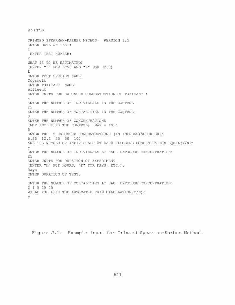
641

A:>TSK

TRIMMED SPEARMAN-KARBER METHOD. VERSION 1.5 ENTER DATE OF TEST: 1 ENTER TEST NUMBER: 2 WHAT IS TO BE ESTIMATED? (ENTER "L" FOR LC50 AND "E" FOR EC50) L ENTER TEST SPECIES NAME: TopsmeltENTER TOXICANT NAME: effluent ENTER UNITS FOR EXPOSURE CONCENTRATION OF TOXICANT : % ENTER THE NUMBER OF INDIVIDUALS IN THE CONTROL: 25 ENTER THE NUMBER OF MORTALITIES IN THE CONTROL: 0 ENTER THE NUMBER OF CONCENTRATIONS (NOT INCLUDING THE CONTROL; MAX = 10): 5 ENTER THE 5 EXPOSURE CONCENTRATIONS (IN INCREASING ORDER): 6.25 12.5 25 50 100ARE THE NUMBER OF INDIVIDUALS AT EACH EXPOSURE CONCENTRATION EQUAL(Y/N)? y ENTER THE NUMBER OF INDIVIDUALS AT EACH EXPOSURE CONCENTRATION: 25 ENTER UNITS FOR DURATION OF EXPERIMENT (ENTER "H" FOR HOURS, "D" FOR DAYS, ETC.): Days ENTER DURATION OF TEST: 7 ENTER THE NUMBER OF MORTALITIES AT EACH EXPOSURE CONCENTRATION: 2 1 5 25 25 WOULD YOU LIKE THE AUTOMATIC TRIM CALCULATION(Y/N)? y

Figure J.1. Example input for Trimmed Spearman-Karber Method.

642

TRIMMED SPEARMAN-KARBER METHOD. VERSION 1.5 DATE: 1 TEST NUMBER: 2 DURATION: 7 Days TOXICANT: effluent SPECIES: Topsmelt RAW DATA: Concentration Number Mortalities --- ---- (%) Exposed .00 25 0 6.25 25 2 12.50 25 1 25.00 25 5 50.00 25 25 100.00 25 25 SPEARMAN-KARBER TRIM: 6.00% SPEARMAN-KARBER ESTIMATES: LC50: 30.98 95% LOWER CONFIDENCE: 27.17 95% UPPER CONFIDENCE: 35.32 NOTE: MORTALITY PROPORTIONS WERE NOT MONOTONICALLY INCREASING. ADJUSTMENTS WERE MADE PRIOR TO SPEARMAN-KARBER ESTIMATION. ------------------------------------------------------------------------------

Figure J.2. Example output for Trimmed Spearman-Karber Method.

643

TABLE K.1. EXAMPLE OF GRAPHICAL METHOD: MORTALITY DATA FROM ATOPSMELT LARVAL SURVIVAL AND GROWTH TEST (25ORGANISMS PER CONCENTRATION)

S))))))))))))))))))))))))))))))))))))))))))))))))))))))))))))))))Q Effluent Number of Mortality Concentration Mortalities Proportion % S))))))))))))))))))))))))))))))))))))))))))))))))))))))))))))))))Q Control 1 0.04 6.25 0 0.00 12.5 0 0.00 25.0 0 0.00 50.0 25 1.00 100.0 25 1.00 S))))))))))))))))))))))))))))))))))))))))))))))))))))))))))))))))Q

APPENDIX K

GRAPHICAL METHOD

1. The Graphical Method is used to calculate the LC50. It is amathematical procedure which estimates the LC50 by linearlyinterpolating between points of a plot of observed percentmortality versus the base 10 logarithm (log10) of percenteffluent concentration. This method does not provide aconfidence interval for the LC50 estimate and its use is onlyrecommended when there are no partial mortalities after the datais smoothed and adjusted for control mortality. The onlyrequirement for the Graphical Method is that the observed percentmortalities bracket 50%.

2. For an analysis using the Graphical Method the data mustfirst be smoothed and adjusted for mortality in the controlreplicates. The procedure for smoothing and adjusting the datais detailed in the following steps.

3. The Graphical Method is illustrated below using a set ofmortality data from a Topsmelt Larval Survival and Growth test. These data are listed in Table K.1.

644

p si&1 ' p s

i ' (pi%pi&1)/2

p s0 ' p s

1 ' p s2 ' p s

3 '0.04 % 0.00 % 0.00 % 0.00

4'

0.044

' 0.01

p ai ' (p s

i &p s0 ) /(1&p s

0 )

4. Let p0, p1, ..., pk denote the observed proportion mortalitiesfor the control and the k effluent concentrations. The firststep is to smooth the pi if they do not satisfy p0 # p1 # ... #pk. The smoothing process replaces any adjacent pi's that do notconform to p0 # p1 # ... # pk with their average. For example, ifpi is less than pi-1 then:

Where: pis = the smoothed observed proportion mortality for effluent concentration i.

4.1 For the data in this example, because the observed mortalityproportions for the 6.25%, 12.5%, and 25.0% effluentconcentrations are less than the observed response proportion forthe control, the values for these four groups must be averaged:

4.2 Since p4 = p5 = 1.00 are larger then 0.01, set p4s = p5s =1.00. Additional smoothing is not necessary. The smoothedobserved proportion mortalities are shown in Table K.2.

5. Adjust the smoothed observed proportion mortality in eacheffluent concentration for mortality in the control group usingAbbott's formula (Finney, 1971). The adjustment takes the form:

Where: p0s = the smoothed observed proportion mortality for the control

pis = the smoothed observed proportion mortality for effluent concentration i.

645

p a0 ' p a

1 ' p a2 ' p a

3 'p s1 & p s

0

1 & p s0

'0.01 & 0.011 & 0.0125

'0.00.99

' 0.0

p a4 ' p a

5 'p s4 & p s

0

1 & p s0

'1.00 & 0.011 & 0.01

'0.990.99

' 1.00

TABLE K.2. EXAMPLE OF GRAPHICAL METHOD: SMOOTHED, ADJUSTEDMORTALITY DATA FROM A TOPSMELT LARVAL SURVIVAL ANDGROWTH TEST

S))))))))))))))))))))))))))))))))))))))))))))))))))))))))))))))))Q Smoothed, Effluent Smoothed Adjusted Concentration Mortality Mortality Mortality % Proportion Proportion Proportion S))))))))))))))))))))))))))))))))))))))))))))))))))))))))))))))))Q Control 0.04 0.01 0.00 6.25 0.00 0.01 0.00 12.5 0.00 0.01 0.00 25.0 0.00 0.01 0.00 50.0 1.00 1.00 1.00 100.0 1.00 1.00 1.00 S))))))))))))))))))))))))))))))))))))))))))))))))))))))))))))))))Q

5.1 Because the smoothed observed proportion mortality for thecontrol group is greater than zero, the responses must beadjusted using Abbott's formula, as follows:

A table of the smoothed, adjusted response proportions for theeffluent concentrations is shown in Table K.2.

5.2 Plot the smoothed, adjusted data on 2-cycle semi-log graphpaper with the logarithmic axis (the y axis) used for percenteffluent concentration and the linear axis (the x axis) used forobserved percent mortality. A plot of the smoothed, adjusteddata is shown in Figure K.1.

646

Figure K.1. Plot of the smoothed adjusted response proportions for topsmelt, Atherinops affinis, survival data.

647

6. Locate the two points on the graph which bracket 50%mortality and connect them with a straight line.

7. On the scale for percent effluent concentration, read thevalue for the point where the plotted line and the 50% mortalityline intersect. This value is the estimated LC50 expressed as apercent effluent concentration.

7.1 For this example, the two points on the graph which bracketthe 50% mortality line (0% mortality at 25% effluent, and 100%mortality at 50% effluent) are connected with a straight line. The point at which the plotted line intersects the 50% mortalityline is the estimated LC50. The estimated LC50 = 35% effluent.

648

APPENDIX L

LINEAR INTERPOLATION METHOD

1. GENERAL PROCEDURE

1.1 The Linear Interpolation Method is used to calculate a pointestimate of the effluent or other toxicant concentration thatcauses a given percent reduction (e.g., 25%, 50%, etc.) in thereproduction or growth of the test organisms (InhibitionConcentration, or IC). The procedure was designed for generalapplicability in the analysis of data from short-term chronictoxicity tests, and the generation of an endpoint from acontinuous model that allows a traditional quantitativeassessment of the precision of the endpoint, such as confidencelimits for the endpoint of a single test, and a mean andcoefficient of variation for the endpoints of multiple tests.

1.2 The Linear Interpolation Method assumes that the responses(1) are monotonically non-increasing, where the mean response foreach higher concentration is less than or equal to the meanresponse for the previous concentration, (2) follow a piecewiselinear response function, and (3) are from a random, independent,and representative sample of test data. If the data are notmonotonically non-increasing, they are adjusted by smoothing(averaging). In cases where the responses at the low toxicantconcentrations are much higher than in the controls, thesmoothing process may result in a large upward adjustment in thecontrol mean. Also, no assumption is made about the distributionof the data except that the data within a group being resampledare independent and identically distributed.

2. DATA SUMMARY AND PLOTS

2.1 Calculate the mean responses for the control and eachtoxicant concentration, construct a summary table, and plot thedata.

3. MONOTONICITY

3.1 If the assumption of monotonicity of test results is met,the observed response means (&Yi) should stay the same or decrease

649

as the toxicant concentration increases. If the means do notdecrease monotonically, the responses are "smoothed" by averaging(pooling) adjacent means.

3.2 Observed means at each concentration are considered in orderof increasing concentration, starting with the control mean (&Y1). If the mean observed response at the lowest toxicantconcentration (&Y2) is equal to or smaller than the control mean(&Y1), it is used as the response. If it is larger than thecontrol mean, it is averaged with the control, and this averageis used for both the control response (M1) and the lowesttoxicant concentration response (M2). This mean is then comparedto the mean observed response for the next higher toxicantconcentration (&Y3). Again, if the mean observed response for thenext higher toxicant concentration is smaller than the mean ofthe control and the lowest toxicant concentration, it is used asthe response. If it is higher than the mean of the first two, itis averaged with the first two, and the mean is used as theresponse for the control and two lowest concentrations oftoxicant. This process is continued for data from the remainingtoxicant concentrations. A numerical example of smoothing thedata is provided below. (Note: Unusual patterns in thedeviations from monotonicity may require an additional step ofsmoothing). Where &Yi decrease monotonically, the &Yi become Miwithout smoothing.

4. LINEAR INTERPOLATION METHOD

4.1 The method assumes a linear response from one concentrationto the next. Thus, the ICp is estimated by linear interpolationbetween two concentrations whose responses bracket the responseof interest, the (p) percent reduction from the control.

4.2 To obtain the estimate, determine the concentrations CJ andCJ+1 which bracket the response M1 (1 - p/100), where M1 is thesmoothed control mean response and p is the percent reduction inresponse relative to the control response. These calculationscan easily be done by hand or with a computer program asdescribed below. The linear interpolation estimate iscalculated as follows:

650

ICp ' CJ % [ M1 (1 & p/100) & MJ ](CJ % 1 & CJ)

(MJ % 1 & MJ)

Where: CJ = tested concentration whose observed meanresponse is greater than M1(1 - p/100).

CJ + 1 = tested concentration whose observed meanresponse is less than M1(1 - p/100).

M1 = smoothed mean response for the control.

MJ = smoothed mean response for concentrationJ.

MJ + 1 = smoothed mean response for concentrationJ + 1.

p = percent reduction in response relativeto the control response.

ICp = estimated concentration at which thereis a percent reduction from the smoothedmean control response. The ICp isreported for the test, together with the95% confidence interval calculated bythe ICPIN.EXE program described below.

4.3 If the CJ is the highest concentration tested, the ICp wouldbe specified as greater than CJ. If the response at the lowestconcentration tested is used to extrapolate the ICp value, theICp should be expressed as a less than the lowest testconcentration.

5. CONFIDENCE INTERVALS

5.1 Due to the use of a linear interpolation technique tocalculate an estimate of the ICp, standard statistical methodsfor calculating confidence intervals are not applicable for theICp. This limitation is avoided by use a technique known as thebootstrap method as proposed by Efron (1982) for deriving pointestimates and confidence intervals.

651

5.2 In the Linear Interpolation Method, the smoothed responsemeans are used to obtain the ICp estimate reported for the test. The bootstrap method is used to obtain the 95% confidenceinterval for the true mean. In the bootstrap method, the testdata Yji is randomly resampled with replacement to produce a newset of data Yji*, that is statistically equivalent to theoriginal data, but a new and slightly different estimate of theICp (ICp*) is obtained. This process is repeated at least 80times (Marcus and Holtzman, 1988) resulting in multiple "data"sets, each with an associate ICp* estimate. The distribution ofthe ICp* estimates derived from the sets of resampled dataapproximates the sampling distribution of the ICp estimate. Thestandard error of the ICp is estimated by the standard deviationof the individual ICp* estimates. Empirical confidence intervalsare derived from the quantiles of the ICp* empiricaldistribution. For example, if the test data are resampled aminimum of 80 times, the empirical 2.5% and the 97.5% confidencelimits are approximately the second smallest and second largestICp* estimates (Marcus and Holtzman, 1988).

5.3 The width of the confidence intervals calculated by thebootstrap method is related to the variability of the data. Whenconfidence intervals are wide, the reliability of the IC estimateis in question. However, narrow intervals do not necessarilyindicate that the estimate is highly reliable, because ofundetected violations of assumptions and the fact that theconfidence limits based on the empirical quantiles of a bootstrapdistribution of 80 samples may be unstable.

5.4 The bootstrapping method of calculating confidence intervalsis computationally intensive. For this reason, all of thecalculations associated with determining the confidence intervalsfor the ICp estimate have been incorporated into a computerprogram. Computations are most easily done with a computerprogram such as the revision of the BOOTSTRP program (USEPA,1988; USEPA, 1989) which is now called "ICPIN" and is describedbelow in subsection 7.

6. MANUAL CALCULATIONS

6.1 DATA SUMMARY AND PLOTS

652

TABLE L.1. MYSID, HOLMESIMYSIS COSTATA, GROWTH DATA)))))))))))))))))))))))))))))))))))))))))))))))))))))))))))))))))))))))))) Concentration (%) Replicate Control 1.80 3.20 5.60 10.0 )))))))))))))))))))))))))))))))))))))))))))))))))))))))))))))))))))))))))) 1 0.048 0.055 0.057 0.041 0.033 2 0.058 0.048 0.050 0.040 0.000 3 0.047 0.042 0.046 0.041 0.000 4 0.058 0.041 0.043 0.043 0.000 5 0.051 0.052 0.045 0.040 0.000))))))))))))))))))))))))))))))))))))))))))))))))))))))))))))))))))))))))))Mean(Y&i) 0.052 0.048 0.048 0.041 0.007i 1 2 3 4 5))))))))))))))))))))))))))))))))))))))))))))))))))))))))))))))))))))))))))

6.1.1 The data used in this example are the mysid growth dataused in the example in Section 14. The data is presented as themean weight per surviving organism. Table L.1 includes the rawdata and the mean growth for each concentration. A plot of thedata is provided in Figure L.1.

6.2 MONOTONICITY

6.2.1. As seen in the table, the observed means aremonotonically non-increasing with respect to concentration. Therefore, the smoothed means will be simply the correspondingobserved mean. The observed means are represented by Y&i and thesmoothed means by Mi. Table L.2 contains the smoothed means andFigure L.1 gives a plot of the smoothed response curve.

6.3 LINEAR INTERPOLATION

6.3.1 An estimates of the IC25 can be calculated using theLinear Interpolation Method. A 25% reduction in mean weight,compared to the controls, would result in a mean weight of 0.039,where M1(1-p/100) = 0.052(1-25/100). Examining the smoothedmeans and their associated concentrations (Table L.2), theresponse, 0.039 mg, is bracketed by C4 = 5.60% and and C5 =10.0%.

653

Figure L.1

. P

lot

of r

aw d

ata,

obs

erve

d me

ans,

and

smo

othe

d me

ans

for

the mysid,

Hol

mesi

msys

cos

tata,

grow

th d

ata.

654

TABLE L.2. MYSID, HOLMESIMYSIS COSTATA, MEAN GROWTH RESPONSE AFTER SMOOTHING S)))))))))))))))))))))))))))))))))))))))))))))))))))))))))))))))))Q

Toxicant Response Smoothed Conc. Means Means (%) i Yi (mg) Mi (mg) S)))))))))))))))))))))))))))))))))))))))))))))))))))))))))))))))))Q Control 1 0.052 0.052 1.80 2 0.048 0.048 3.20 3 0.048 0.048 5.60 4 0.041 0.041 10.00 5 0.007 0.007 18.00 6 0.000 0.000 S)))))))))))))))))))))))))))))))))))))))))))))))))))))))))))))))))Q

6.3.2 Using the equation from section 4.2, the estimate of theIC25 is calculated as follows:

ICp ' CJ % [ M1 (1 & p/100) & MJ ]

(CJ % 1 & CJ)

(MJ % 1 & MJ)

IC25 ' 5.60 % [0.052 (1 & 25/100) & 0.041] (10.0 & 5.60)(0.007 & 0.041)

= 5.86%

6.4 CONFIDENCE INTERVALS

6.4.1 Confidence intervals for the ICp are derived using thebootstrap method. As described above, this method involvesrandomly resampling the individual observations and recalculatingthe ICp at least 80 times, and determining the mean ICp, standarddeviation, and empirical 95% confidence intervals. For thisreason, the confidence intervals are calculated using a computerprogram called ICPIN. This program is described below and isavailable to carry out all the calculations of both theinterpolation estimate (ICp) and the confidence intervals.

655

7. COMPUTER CALCULATIONS

7.1 The computer program, ICPIN, prepared for the LinearInterpolation Methods was written in TURBO PASCAL for IBMcompatible PCs. The program (version 2.0) has been modified byComputer Science Corporation, Duluth, MN with funding provided bythe Environmental Research Laboratory, Duluth, MN (Norberg-King,1993). The program was originally developed by BattelleLaboratories, Columbus, OH through a government contractsupported by the Environmental Research Laboratory, Duluth, MN(USEPA, 1988). A compiled, executable version of the program andsupporting documentation can be obtained by sending a writtenrequest to EMSL-Cincinnati, 3411 Church Street, Cincinnati, OH 45244.

7.2 The ICPIN.EXE program performs the following functions: 1)it calculates the observed response means (Yi) (response means); 2) it calculates the standard deviations; 3) checks theresponses for monotonicity; 4) calculates smoothed means (Mi)(pooled response means) if necessary; 5) uses the means, Mi, tocalculate the initial ICp of choice by linear interpolation; 6)performs a user-specified number of bootstrap resamples between80 and 1000 (as multiples of 40); 7) calculates the mean andstandard deviation of the bootstrapped ICp estimates; and 8)provides an original 95% confidence intervals to be used with theinitial ICp when the number of replicates per concentration isover six and provides both original and expanded confidenceintervals when the number of replicates per concentration areless than seven (Norberg-King, 1993).

7.3 For the ICp calculation, up to twelve treatments can beinput (which includes the control). There can be up to 40replicates per concentration, and the program does not require anequal number of replicates per concentration. The value of p canrange from 1% to 99%.

7.4 DATA INPUT

7.4.1 Data is entered directly into the program onscreen. Asample data entry screen in shown in Figure L.2. The programdocumentation provides guidance on the entering and analysis ofdata for the Linear Interpolation Method.

656

ICp Data Entry/Edit Screen Current File: Conc. ID * 1 * 2 * 3 * 4 * 5 * 6 Conc. Tested * * * * * * Response 1 * * * * * * Response 2 * * * * * * Response 3 * * * * * * Response 4 * * * * * * Response 5 * * * * * * Response 6 * * * * * * Response 7 * * * * * * Response 8 * * * * * * Response 9 * * * * * * Response 10 * * * * * * Response 11 * * * * * * Response 12 * * * * * * Response 13 * * * * * * Response 14 * * * * * * Response 15 * * * * * * Response 16 * * * * * * Response 17 * * * * * * Response 18 * * * * * * Response 19 * * * * * * Response 20 * * * * * * 44444444444444444444444444444444444444444444444444444444444444444444444444F10 for Command Menu Use Arrow Keys to Switch Fields

Figure L.2. ICp data entry/edit screen. Twelve concentrationidentifications can be used. Data for concentrationsare entered in columns 1 through 6. For concentrations

657

7.4.2 The user selects the ICp estimate desired (e.g., IC25 orIC50) and the number of resamples to be taken for the bootstrapmethod of calculating the confidence intervals. The program hasthe capability of performing any number of resamples from 80 to1000 as multiples of 40. However, Marcus and Holtzman (1988)recommend a minimum of 80 resamples for the bootstrap method beused and at least 250 resamples are better (Norberg-King, 1993).

7.5 DATA OUTPUT

7.5.1 The program output includes the following (see Figure L.3)

1. A table of the concentration identification, theconcentration tested and raw data response for eachreplicate and concentration.

2. A table of test concentrations, number of replicates,concentration (units), response means (Yi), standarddeviations for each response mean, and the pooledresponse means (smoothed means; Mi).

3. The linear interpolation estimate of the ICp using themeans (Mi). Use this value for the ICp estimate.

4. The mean ICp and standard deviation from the bootstrapresampling.

5. The confidence intervals calculated by the bootstrapmethod for the ICp. Provides an original 95% confidenceintervals to be used with the initial ICp when the numberof replicates per concentration is over six and providesboth original and expanded confidence intervals when thenumber of replicates per concentration are less thanseven.

7.6 ICPIN program output for the analysis of the mysid growthdata in Table L.1 is provided in Figure L.3.

7.6.1 When the ICPIN program was used to analyze this set ofdata, requesting 80 resamples, the estimate of the IC25 was5.8174%. The empirical 95% confidence intervals for the truemean was 4.9440% to 6.2553%.

658

Conc. ID 1 2 3 4 5 6------------------------------------------------------------------------Conc. Tested 0 1.80 3.20 5.60 10.0 18.0------------------------------------------------------------------------Response 1 .048 .055 .057 .041 .033 0Response 2 .058 .048 .050 .040 0 0Response 3 .047 .042 .046 .041 0 0Response 4 .058 .041 .043 .043 0 0Response 5 .051 .052 .045 .040 0 0------------------------------------------------------------------------*** Inhibition Concentration Percentage Estimate ***Toxicant/Effluent: EffluentTest Start Date: Test Ending Date: Test Species: mysid, Holmesimysis costataTest Duration: 7 daysDATA FILE: mysid.icpOUTPUT FILE: mysid.i25-----------------------------------------------------------------------Conc. Number Concentration Response Std. Pooled ID Replicates % Means Dev. Response Means----------------------------------------------------------------------- 1 5 0.000 0.052 0.005 0.052 2 5 1.800 0.048 0.006 0.048 3 5 3.200 0.048 0.006 0.048 4 5 5.600 0.041 0.001 0.041 5 5 10.000 0.007 0.015 0.007 6 5 18.000 0.000 0.000 0.000-----------------------------------------------------------------------The Linear Interpolation Estimate: 5.8174 Entered P Value: 25-----------------------------------------------------------------------Number of Resamplings: 80The Bootstrap Estimates Mean: 5.8205 Standard Deviation: 0.2673Original Confidence Limits: Lower: 4.9440 Upper: 6.2553Expanded Confidence Limits: Lower: 4.5073 Upper: 6.4743Resampling time in Seconds: 0.22 Random_Seed: 526805435

Figure L.3. Example of ICPIN program output for the IC25.

659

CITED REFERENCES

Bartlett, M.S. 1937. Some examples of statistical methods ofresearch in agriculture and applied biology. J. RoyalStatist. Soc. Suppl. 4:137-183.

Conover, W.J. 1980. Practical nonparametric statistics. Secondedition. John Wiley and Sons, NY, NY. pp. 466-467.

Dixon, W.J., and F.J. Massey, Jr. 1983. Introduction tostatistical analysis. Fourth Edition. McGraw Hill, NY, NY.

Draper, N.R., and J.A. John. 1981. Influential observations andoutliers in regression. Technometrics 23:21-21.

Dunnett, C.W. 1955. Multiple comparison procedure for comparingseveral treatments with a control. J. Amer. Statist.Assoc. 50:1096-1121.

Dunnett, C.W. 1964. New table for multiple comparisons with acontrol. Biometrics 20:482.

Efron, B. 1982. The Jackknife, the Bootstrap, and otherresampling plans. CBMS 38, Soc. Industr. Appl. Math.,Philadelphia, PA.

Finney, D.J. 1971. Probit analysis. Third Edition. CambridgePress, NY, NY. 668 pp.

Finney, D.J. 1978. Statistical method in biological assay. Third Edition. Charles Griffin & Co. Ltd, London, England.508 pp.

Hamilton, M.A., R.C. Russo, and R.V. Thurston. 1977. TrimmedSpearman-Karber method for estimating median lethalconcentrations. Environ. Sci. Tech. 11(7):714-719.

Marcus, A.H., and A.P. Holtzman. 1988. A robut statisticalmethod for estimating effects concentrations in short-termfathead minnow toxicity tests. Manuscript submitted to theCriteria and Standards Division, U. S. EnvironmentalProtection Agency, by Battelle Washington Environmental

660

Program Office, Washington, DC. June 1988 under EPA ContractNo. 69-03-3534. 39 pp.

Miller, R.G. 1981. Simultaneous statistical inference. Springer-Verlag, New York, NY. 299 pp.

Norberg-King, T.J. 1993. A linear interpolation method forsublethal toxicity: The inhibition concentration (ICp)approach. Version 2.0. National Effluent ToxicityAssessment Center Technical Report 03-93, EnvironmentalResearch Laboratory, Duluth, MN 55804. June 1993

Scheffe, H. 1959. The analysis of variance. John Wiley, NewYork. 477 pp.

Snedecor, G.W., and W.G. Cochran. 1980. Statistical Methods. Seventh edition. Iowa State University Press, Ames, IA. 593 pp.

Steel, R.G. 1959. A multiple comparison rank sum test:treatments versus control. Biometrics 15:560-572.

Stephens, M.A. 1974. EDF statistics for goodness of fit andcome comparisons. J. Amer. Stat. Assoc. (JASA) 69:730-7737.

USEPA. 1988. An interpolation estimate for chronic toxicity:The ICp approach. Norberg-King, T.J. Technical Report 05-88, National Effluent Toxicity Assessment Center,Environmental Research Laboratory, U. S. EnvironmentalProtection Agency, Duluth, MN 55804.

USEPA. 1989. Short-term methods for estimating the chronictoxicity of effluents and receiving waters to freshwaterorganisms. Second Edition. Weber, C.I., W.H. Peltier, T.J.Norberg-King, W.B. Horning, II, F.A. Kessler, J.R.Menkedick, T.W. Neiheisel, P.A. Lewis, D.J. Klemm, Q.H.Pickering, E.L. Robinson, J.M. Lazorchak, L.J. Wymer, andR.W. Freyberg (eds.). Environmental Monitoring SystemsLaboratory, U. S. Environmental Protection Agency,Cincinnati, OH 45268. EPA/600/4-89/001.

USEPA. 1993. Methods for measuring the acute toxicity ofeffluents and receiving waters to freshwater and marine

661

organisms. Fourth Edition. Weber, C.I. (ed.). Environmental Monitoring Systems Laboratory, U. S.Environmental Protection Agency, Cincinnati, OH 45268.EPA/600/4-90/027F.