Attitude Determination of a Land Vehicle usingInertial Measurement Units

By:

Brian Bleeker- bbleeker_02@yahoo.comRob MacMillan- cubsfan789@yahoo.com

Advised by:

Dr. In Soo Ahn

Date:

May 12, 2003

2

Table of Contents

1. PROJECT SUMMARY 3

2. PROJECT DESCRIPTION 3-82.1. Inertial Measurement Unit 3-42.2. Attitude Computer 4-52.3. Resolution of Specific Forces 42.4. Navigation Computer 5-62.5. Completed Work 6-7

2.5.1. Product Research 6-72.5.2. Practice Matlab Code 72.5.3. Attitude Computer Matlab Code 7

2.6. Experimental Testing 7-8

3. TESTS AND RESULTS 9-163.1. Initial IMU Testing 9-103.2. Euler Angle Initialization 10-123.3. Euler Angle Computation 123.4. Filtering Methods 12-143.5. Position Calculation 14-16

4. STANDARDS/PATENTS 16-174.1. Standards 16-174.2. Patents 17

5. EQUIPMENT LIST 17

6. CONCLUSIONS 17

APPENDIX A Practice Matlab Code: 18-22ECEF to NED Coordinates 18-20NED to ECEF Coordinates 21-22

APPENDIX B Overall System Matlab Code: 23-36Earth Parameters 23Turn Rate of Earth 23Turn Rate of Navigation Frame 24Turn Rate of the Body in the Body Frame 24Skew Matrix 25Update Directional Cosine Matrix 25Gravity Computer 25Covariance Filter 26-28Cbn Initialization 28-29Euler Angle Computation 29Average/Velocity Slope Filter 29-31Navigation Equation - Determine Position 31-32Determine Latitude, Longitude, and Attitude 32Main Program 32-36

REFERENCE 37

3

1. Project Summary

To determine the attitude of a land vehicle with respect to navigation coordinates, angularrates and translational accelerations are measured using an inertial measurement unit(IMU). This attitude and position determination system can function as a stand-alonesystem or supplement a global positioning system in time when there is no line of sight toGPS satellites. Similar systems can be implemented to record the movement of thevehicle to prevent it from leaving a set course or from moving into an unstable ordangerous environment. These systems may help a driver by triggering increasedtraction control and air bag deployment as the accelerations and attitude angles changewhile driving. The block diagram of this system is shown in Fig. 1.1.1.

body mounted

gyroscopes

resolution of specific forces

attitude computer

Σ body

mounted accelerometers

Coriolis correction

gravity computer

initial estimates of

attitude

position & velocity

estimates

Σ fb

ωib

navigation computer

Figure 1.1.1 Overall Block Diagram of the system

2. Project Description

2.1. Inertial Measurement Unit

Movement of the land vehicle causes the output of the three accelerometers and threegyroscopes within the IMU to output the translational accelerations and angular rateswith respect to the body axis. Gravity is shown as acceleration on one or more of theacceleration outputs depending upon how the IMU is attached to the land vehicle (seefigure 2.1.1).

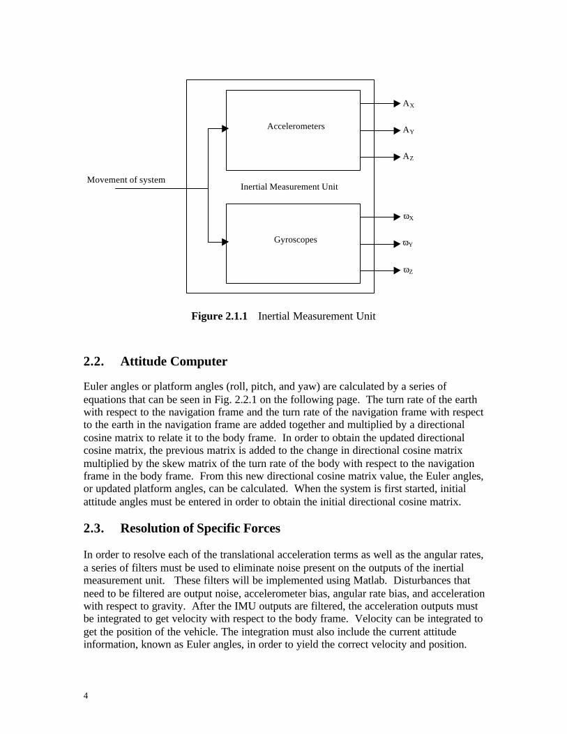
4

Figure 2.1.1 Inertial Measurement Unit

2.2. Attitude Computer

Euler angles or platform angles (roll, pitch, and yaw) are calculated by a series ofequations that can be seen in Fig. 2.2.1 on the following page. The turn rate of the earthwith respect to the navigation frame and the turn rate of the navigation frame with respectto the earth in the navigation frame are added together and multiplied by a directionalcosine matrix to relate it to the body frame. In order to obtain the updated directionalcosine matrix, the previous matrix is added to the change in directional cosine matrixmultiplied by the skew matrix of the turn rate of the body with respect to the navigationframe in the body frame. From this new directional cosine matrix value, the Euler angles,or updated platform angles, can be calculated. When the system is first started, initialattitude angles must be entered in order to obtain the initial directional cosine matrix.

2.3. Resolution of Specific Forces

In order to resolve each of the translational acceleration terms as well as the angular rates,a series of filters must be used to eliminate noise present on the outputs of the inertialmeasurement unit. These filters will be implemented using Matlab. Disturbances thatneed to be filtered are output noise, accelerometer bias, angular rate bias, and accelerationwith respect to gravity. After the IMU outputs are filtered, the acceleration outputs mustbe integrated to get velocity with respect to the body frame. Velocity can be integrated toget the position of the vehicle. The integration must also include the current attitudeinformation, known as Euler angles, in order to yield the correct velocity and position.

Inertial Measurement UnitMovement of system

Accelerometers

Gyroscopes

AX

AY

AZ

ωX

ωY

ωZ

5

Figure 2.2.1 Attitude Computer

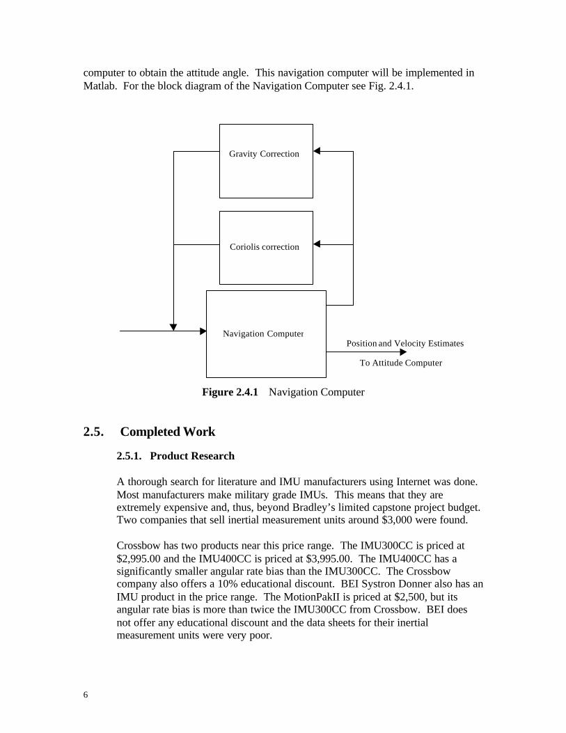
2.4. Navigation Computer

In order to properly compute the attitude of the land vehicle, the attitude computer mustbe updated continuously as the vehicle moves. Also, gravity and Coriolis force must beproperly factored in to give velocity and position estimates in the local navigation system.With these corrections the movement of the land vehicle can be fed back to the attitude

Get raw angular data from IMUbibω

Compute:nenωnieω

Compute:

[ ]nie

nen

nb

bib

bnb C ωωωω +−=

Obtain the initial attitudeangles

UpdatedPlatform Angles

000 ,, γβα

Initial:

)0(nbC

Update nbC :

[ ])()()()( ttCttCttC bnb

nb

nb

nb Ω∆+=∆+

Skew Matrix:

][ bnb

bnb skew ω=Ω

Earth DataRo

L, altitude

6

computer to obtain the attitude angle. This navigation computer will be implemented inMatlab. For the block diagram of the Navigation Computer see Fig. 2.4.1.

Figure 2.4.1 Navigation Computer

2.5. Completed Work

2.5.1. Product Research

A thorough search for literature and IMU manufacturers using Internet was done.Most manufacturers make military grade IMUs. This means that they areextremely expensive and, thus, beyond Bradley’s limited capstone project budget.Two companies that sell inertial measurement units around $3,000 were found.

Crossbow has two products near this price range. The IMU300CC is priced at$2,995.00 and the IMU400CC is priced at $3,995.00. The IMU400CC has asignificantly smaller angular rate bias than the IMU300CC. The Crossbowcompany also offers a 10% educational discount. BEI Systron Donner also has anIMU product in the price range. The MotionPakII is priced at $2,500, but itsangular rate bias is more than twice the IMU300CC from Crossbow. BEI doesnot offer any educational discount and the data sheets for their inertialmeasurement units were very poor.

Navigation Computer

Gravity Correction

Coriolis correction

Position and Velocity Estimates

To Attitude Computer

7

These products are significantly less expensive than military grade productsbecause they are manufactured with silicon chips. These chips are prone toincreased biases and random walk noise. For the purposes of this project theIMU300CC was purchased.

2.5.2. Practice Matlab Code

To get familiar with writing Matlab functions, sample data taken from a GPSreceiver was analyzed. The data file was read into Matlab. This data was inearth-centered earth fixed coordinates. This means that the location of thereceiver was measured with respect to the center of the earth. The goal of theexercise was to convert the ECEF coordinates to local navigation coordinates.Also, another function was written to convert the local navigation coordinatesback to the ECEF coordinates. The Matlab code written for this exercise and theresults from the code are attatched in Appendix A.

2.5.3. Attitude Computer Matlab Code

The attitude computer of the attitude determination system is written andfunctional. Each block of the diagram is written as individual functions. Thiswill help in writing other programs so that each function can be calledaccordingly. The following list of code has been written and attached inAppendix B.Ø The turn rate of the navigation frame with respect to the earth in the

navigation frame.Ø The turn rate of the earth with respect to the inertial frame in the

navigation frame.Ø The turn rate of the body frame with respect to the navigation frame in the

body frame.Ø Skew symmetric matrix for a 1 by 3 column vector.Ø Update the directional cosine matrix of the body frame in the navigation

frame.Ø Initialize the directional cosine matrix.Ø Create the current platform angles.

With all these functions written an overall main file was written to call thefunctions of the attitude computer. This function will also control the transfer ofdata between the resolution of specific forces, navigation computer and attitudecomputer.

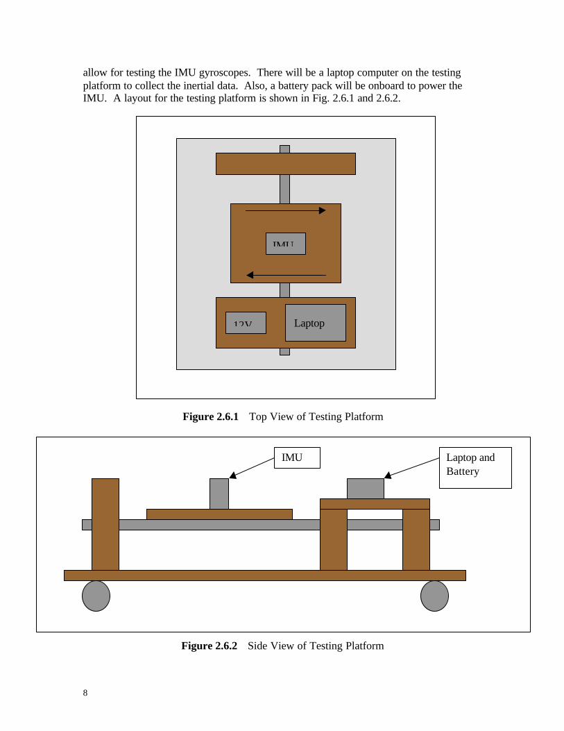
2.6. Experimental Testing

To simulate the movements of a land-based vehicle, a tested platform will be constructed.This platform will have wheels to allow the user to push it in the desired direction to testthe IMU accelerometers. The testing platform will also have a rotating axis that will

8

IMU

12V Laptop

allow for testing the IMU gyroscopes. There will be a laptop computer on the testingplatform to collect the inertial data. Also, a battery pack will be onboard to power theIMU. A layout for the testing platform is shown in Fig. 2.6.1 and 2.6.2.

Figure 2.6.1 Top View of Testing Platform

Figure 2.6.2 Side View of Testing Platform

Laptop andBattery

IMU

9

3. Tests and Results

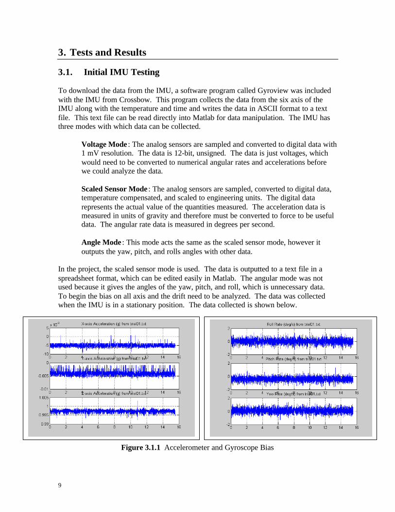
3.1. Initial IMU Testing

To download the data from the IMU, a software program called Gyroview was includedwith the IMU from Crossbow. This program collects the data from the six axis of theIMU along with the temperature and time and writes the data in ASCII format to a textfile. This text file can be read directly into Matlab for data manipulation. The IMU hasthree modes with which data can be collected.

Voltage Mode : The analog sensors are sampled and converted to digital data with1 mV resolution. The data is 12-bit, unsigned. The data is just voltages, whichwould need to be converted to numerical angular rates and accelerations beforewe could analyze the data.

Scaled Sensor Mode : The analog sensors are sampled, converted to digital data,temperature compensated, and scaled to engineering units. The digital datarepresents the actual value of the quantities measured. The acceleration data ismeasured in units of gravity and therefore must be converted to force to be usefuldata. The angular rate data is measured in degrees per second.

Angle Mode : This mode acts the same as the scaled sensor mode, however itoutputs the yaw, pitch, and rolls angles with other data.

In the project, the scaled sensor mode is used. The data is outputted to a text file in aspreadsheet format, which can be edited easily in Matlab. The angular mode was notused because it gives the angles of the yaw, pitch, and roll, which is unnecessary data.To begin the bias on all axis and the drift need to be analyzed. The data was collectedwhen the IMU is in a stationary position. The data collected is shown below.

Figure 3.1.1 Accelerometer and Gyroscope Bias

10

From figure 3.1.1 it is determined that all of the axes of the IMU are extremely noisy andhave significant bias.

3.2. Euler Angle Initialization

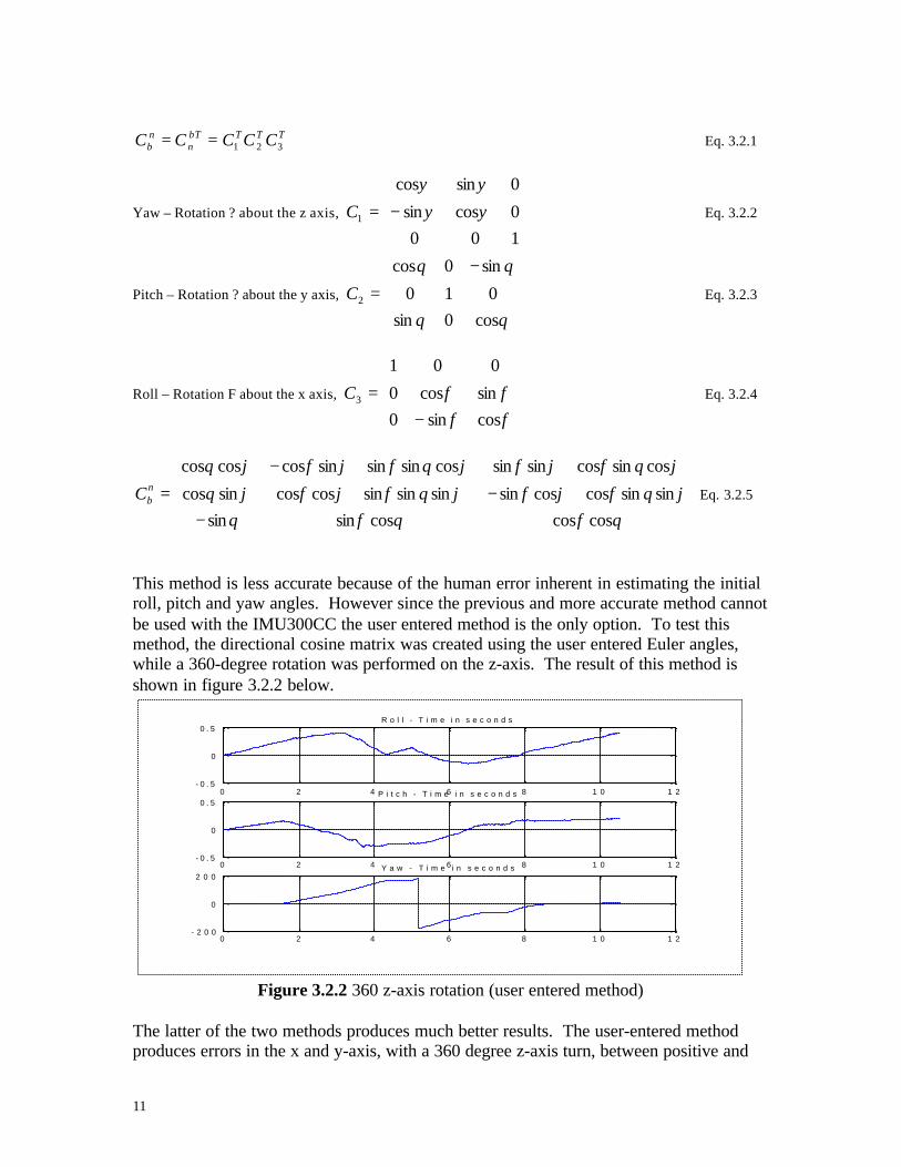
In order to initialize the Euler angles in an inertial measurement system, the data from theaccelerometers and gyroscopes are compared to the known quantity of the rotation of theearth and local gravity calculated in the gravity computer. Because the data shown infigure 3.1.1 has such a large bias and is very noisy, it is impossible to determine therotation of the earth and gravity from the given data. To test this method, the directionalcosine matrix was created using this process while a 360-degree rotation was performedon the z-axis. The result of this method is shown in figure 3.2.1 below.

Figure 3.2.1 360-degree z axis rotation(earth rotation and gravity method)

From the data shown in figure 3.2.1, the z axis does rotate 360 degrees however there isundesired rotation on both the x and y axis. This shows the failure of the earth rotationand gravity method to initialize the directional cosine matrix. To prove that isinitialization method does not work in this situation the norm of the direction cosinematrix in every time step should be approximately 1. The norm turned out to be muchgreater than 1 and is useless.

Cbn =39.36 129.38 46.68127.86 -39.89 -1.13-2.03 -4.88 -2.73

Norm(Cbn) = 141.89

To initialize the directional cosine matrix to one that will work in this situation, the usermust enter the initial roll, pitch and yaw angles. From the user inputs, a directionalcosine matrix is formed using the following equations.

11

TTTbTn

nb CCCCC 321== Eq. 3.2.1

Yaw – Rotation ? about the z axis,

−=

1000cossin

0sincos

1 ψψ

ψψ

C Eq. 3.2.2

Pitch – Rotation ? about the y axis,

−

=θθ

θθ

cos0sin010

sin0cos

2C Eq. 3.2.3

Roll – Rotation F about the x axis,

−=

φφφφ

cossin0sincos0

001

3C Eq. 3.2.4

−+−+

++−

=θφθφθ

ϕθφϕφϕθφϕφϕθ

ϕθφϕφϕθφϕφϕθ

coscoscossinsinsinsincoscossinsinsinsincoscossincos

cossincossinsincossinsinsincoscoscosnbC Eq. 3.2.5

This method is less accurate because of the human error inherent in estimating the initialroll, pitch and yaw angles. However since the previous and more accurate method cannotbe used with the IMU300CC the user entered method is the only option. To test thismethod, the directional cosine matrix was created using the user entered Euler angles,while a 360-degree rotation was performed on the z-axis. The result of this method isshown in figure 3.2.2 below.

Figure 3.2.2 360 z-axis rotation (user entered method)

The latter of the two methods produces much better results. The user-entered methodproduces errors in the x and y-axis, with a 360 degree z-axis turn, between positive and

0 2 4 6 8 1 0 1 2- 0 . 5

0

0 . 5R o l l - T i m e i n s e c o n d s

0 2 4 6 8 1 0 1 2- 0 . 5

0

0 . 5P i t c h - T i m e i n s e c o n d s

0 2 4 6 8 1 0 1 2- 2 0 0

0

2 0 0Y a w - T i m e i n s e c o n d s

12

negative 0.5 degrees. There is, however, a significant error and further filtering on allaxes is required. The filtering methods are discussed in Section 3.4.

3.3. Euler Angle ComputationThe Euler angles are computed directly from the directional cosine matrix after everyupdate. The angles are computed using a series of equations shown below.

Roll:

=33

32arctanCC

φ Eq. 3.3.1

Pitch: 31arcsin C−=θ Eq. 3.3.2

Yaw:

=11

21arctanCC

ϕ Eq. 3.3.3

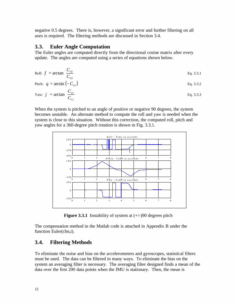
When the system is pitched to an angle of positive or negative 90 degrees, the systembecomes unstable. An alternate method to compute the roll and yaw is needed when thesystem is close to this situation. Without this correction, the computed roll, pitch andyaw angles for a 360-degree pitch rotation is shown in Fig. 3.3.1.

Figure 3.3.1 Instability of system at (+/-)90 degrees pitch

The compensation method in the Matlab code is attached in Appendix B under thefunction Euler(cbn,i).

3.4. Filtering Methods

To eliminate the noise and bias on the accelerometers and gyroscopes, statistical filtersmust be used. The data can be filtered in many ways. To eliminate the bias on thesystem an averaging filter is necessary. The averaging filter designed finds a mean of thedata over the first 200 data points when the IMU is stationary. Then, the mean is

0 1 2 3 4 5 6 7 8- 4 0 0

- 2 0 0

0

2 0 0R o l l - T i m e i n s e c o n d s

0 1 2 3 4 5 6 7 8- 1 0 0

0

1 0 0P i t c h - T i m e i n s e c o n d s

0 1 2 3 4 5 6 7 8- 2 0 0

0

2 0 0Y a w - T i m e i n s e c o n d s

13

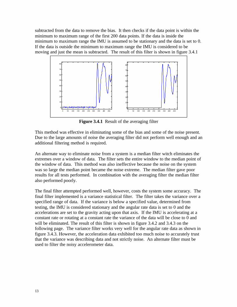
subtracted from the data to remove the bias. It then checks if the data point is within theminimum to maximum range of the first 200 data points. If the data is inside theminimum to maximum range the IMU is assumed to be stationary and the data is set to 0.If the data is outside the minimum to maximum range the IMU is considered to bemoving and just the mean is subtracted. The result of this filter is shown in figure 3.4.1

Figure 3.4.1 Result of the averaging filter

This method was effective in eliminating some of the bias and some of the noise present.Due to the large amounts of noise the averaging filter did not perform well enough and anadditional filtering method is required.

An alternate way to eliminate noise from a system is a median filter witch eliminates theextremes over a window of data. The filter sets the entire window to the median point ofthe window of data. This method was also ineffective because the noise on the systemwas so large the median point became the noise extreme. The median filter gave poorresults for all tests performed. In combination with the averaging filter the median filteralso performed poorly.

The final filter attempted performed well, however, costs the system some accuracy. Thefinal filter implemented is a variance statistical filter. The filter takes the variance over aspecified range of data. If the variance is below a specified value, determined fromtesting, the IMU is considered stationary and the angular rate data is set to 0 and theaccelerations are set to the gravity acting upon that axis. If the IMU is accelerating at aconstant rate or rotating at a constant rate the variance of the data will be close to 0 andwill be eliminated. The result of this filter is shown in figure 3.4.2 and 3.4.3 on thefollowing page. The variance filter works very well for the angular rate data as shown infigure 3.4.3. However, the acceleration data exhibited too much noise to accurately trustthat the variance was describing data and not strictly noise. An alternate filter must beused to filter the noisy accelerometer data.

0 50 100 150 200 250 300 350 400 450

0

10

20

30

40

50

60

70

80

0 50 100 150 200 250 300 350 400 450

0

10

20

30

40

50

60

70

80

14

Figure 3.4.2 Stationary IMU Roll, Pitch and Yaw Results using Variance Filter

Figure 3.4.3 360-Degree Yaw Rotation Unfiltered(left) and Variance Filtered(right)

3.5 Position Calculation

In order to convert acceleration data to velocity and position, two integrations factoring inthe necessary corrections must be performed; integrating acceleration produces velocityand integrating velocity produces position. The corrections that must be accounted forwhen integrating velocity include: subtracting the force of gravity on the z-axis,subtracting the Coriolis effect (the rotation of the earth), and updating the change inattitude given by the directional cosine matrix. However, when integrating theacceleration twice, any bias seen on those axis will produce a quadratic function seen inthe position. Also, any noise on the outputs of the accelerometers will distort the positionof the vehicle. As discussed above, the filtering methods worked well for the rotation rateoutputs from the three inertial gyroscopes, however, they were ineffective for the threeoutputs from the accelerometers. The filters were ineffective because the bias on theaccelerometers has a random value when powered up and changes values as the systemmoves. The changing bias along with the random startup value disallows a directsubtraction of the bias at the input of the system. There is also significant noise on theaccelerometers. This noise increases in size when the inertial measurement unit is moved

0 5 0 0 1 0 0 0 1 5 0 0 2 0 0 0 2 5 0 0-1

0

1R o l l - T i m e i n s e c o n d s

0 5 0 0 1 0 0 0 1 5 0 0 2 0 0 0 2 5 0 0-1

0

1P i t c h - T i m e i n s e c o n d s

0 5 0 0 1 0 0 0 1 5 0 0 2 0 0 0 2 5 0 0- 2 0 0

0

2 0 0Y a w - T i m e i n s e c o n d s

0 2 0 0 4 0 0 6 0 0 8 0 0 1 0 0 0 1 2 0 0 1 4 0 0-1

0

1R o l l - T i m e i n s e c o n d s

0 2 0 0 4 0 0 6 0 0 8 0 0 1 0 0 0 1 2 0 0 1 4 0 0-1

0

1P i t c h - T i m e i n s e c o n d s

0 2 0 0 4 0 0 6 0 0 8 0 0 1 0 0 0 1 2 0 0 1 4 0 0-1

0

1Y a w - T i m e i n s e c o n d s

0 2 4 6 8 1 0 1 2- 0 . 5

0

0 . 5R o l l - T i m e i n s e c o n d s

0 2 4 6 8 1 0 1 2- 0 . 5

0

0 . 5P i t c h - T i m e i n s e c o n d s

0 2 4 6 8 1 0 1 2- 2 0 0

0

2 0 0Y a w - T i m e i n s e c o n d s

15

or rotated on any axis even if the movement or rotation is not on the axis being looked at.Both the changing bias and the increased noise can be seen in figure 3.5.1 below.

Figure 3.5.1 Changing Bias and increased noise on X-axis, No movement on X-axishowever rotation on Z-axis

In figure 3.5.1 the noise is very large which would indicate some movement in the Xdirection. There was however no movement in the X direction, only a rotation about theZ-axis(Yaw). Some of the increase in noise may be attributed to centripetal force,however, because the rotation of the body is fairly slow, the centripetal force should notcontribute that much to the acceleration along the X-axis. Also, in figure 3.5.1, thechanging bias can be seen. The bias in this case ranges from about 0.1G to about -0.05G. This seemingly random change in bias has no pattern and cannot be predicted.The bias change on all three accelerometer axis does not depend on the type of movementor the axis on which the movement occurs.When integrated, the noise and the bias on the accelerometers produces an unwantedlinear velocity as shown in figure 3.5.2 on the following page. Using the first 200stationary data points on each axis, the slope of the linear velocity is computed andsubtracted directly from the velocity of the entire data set on their respective axis. Thisprovides some correction and improves the output of the position of the vehicle. Therandom bias on the system however is a very large problem. Shown in figure 3.5.3 and3.5.4 on the following page are the results of moving the inertial measurement unit onemeter north and then one meter south. Because the bias of the system changes, themovement north is not equivalent to the movement south. When there is no movement atall, the system shows a constant positive velocity. When integrated, this constant positivevelocity becomes a linear change in position. Due to the excessive noise and randombias, position and velocity could not be determined using this inertial measurement unit.

Changing bias

16

Figure 3.5.2 Unwanted linear velocity on stationary test

Figure 3.5.3 and 3.5.4 Velocity and position of system with random bias

4. Standards/Patents

4.1 Standards

A standard search was done on the Internet. Places to purchase standards were found, butthere were no free standards listings found. As of right now, standards have not beenpurchased for this project.

4.2 Patents

Using a patent research tool linked to the Bradley University Cullom Davis Librarywebsite the following patents have similarities to this project.

17

Ø 6,463,366 Attitude determination and alignment using electro-optical sensorsand global navigation satellites

Ø 6,417,802 Integrated inertial/GPS navigation system

Ø 6,292,750 Vehicle positioning method and system thereof

All of the above patents have to do with a system integrating a GPS receiver and aninertial measurement unit. For these systems the GPS acts to initialize and keep the IMUwithin error specs by resetting the system. This project does not depend on the errorcompensation abilities of the GPS systems. As of right now, there are no patents directlyapplicable to this project.

5. Equipment List

1 – Inertial Measurement Unit1 – Laptop computer1 – 12V battery1 – Testing Platform

6. Conclusions

The overall goal of the project was to determine the attitude of a vehicle using the inputsfrom the inertial measurement unit. The project goal was completed successfully. As anextension of this project, determining the position of the inertial measurement unit wasattempted for complete inertial navigation solutions. However, due to the excessive noiseand random bias of the Crossbow IMU, position determination and, hence, a completenavigation solution is not possible with this IMU unless a separate sensor like agyrocompass is used for a proper initialization. Although complete inertial navigation isnot possible, this IMU can be applied to some useful short-term applications for detectingaccelerations and velocities.

18

APPENDIX A – Practice Matlab Code

The following is code for Matlab converting the position ofa vehicle in earth-centered earth fixed coordinates toLatitude Longitude and altitude.Figure A.1 shows the position in ECEF coordinatesFigure A.2 shows the position in latitude, longitude andaltitude

From the website http:// www.geocode.com/eagle.html it wasfound that the approximate address where the data was takewas 1701 E. Empire St. in Bloomington Il.

ECEF To NEDfunction [lat, lon, alt] = ecef2ned(gtime, ecefpos)

% ECEF2NED Convert ecef coordinates to NED coordinates and diplay.%% [latitude, longitude, altitude] = ecef2ned(gtime, ECEF position)% ECEF Position Array = [x, y, z]%% Example:% array.x% array.y% array.z% *** The array parameters must have *.x, *.y, and *.z.%% Enter the time, and the x,y,z positions in ecef coordinates.% This function will display two figures:% 1: x,y,z position in ecef coordinates and% 2: latitude, longitude, and altitude% A negative longitude is the Western hemispere.% A negative latitude is in the Southern hemisphere.%% Written By: Brian Bleeker% Rob MacMillan

b = size(gtime);gtime = gtime(:,1) - gtime(1,1);

figure(1), subplot(311), plot(gtime, ecefpos.x), gridtitle('ECEF X Position')

subplot(312), plot(gtime, ecefpos.y), gridtitle('ECEF Y Position')

subplot(313), plot(gtime, ecefpos.z), gridtitle('ECEF Z Position')

a = 6378137.0; %semi-major axis(equatorial) radiusb = 6356752.3142; %semi-minor axis(polar) radius

19

f = (a-b)/a;e = sqrt(f*(2-f)); %eccentricity ofellipsoidlen = length(ecefpos.x); %get length of data

for i = 1:len lon(i) = atan2(ecefpos.y(i), ecefpos.x(i)); %long = atan(y,x) -direct lon(i) = lon(i)*180/pi; %convert to degrees

h = 0; %initialize N = a; flag = 0; j = 0; p = sqrt(ecefpos.x(i)^2 + ecefpos.y(i)^2);

sinlat = ecefpos.z(i)/(N*(1-e^2)+h); %First iteration lat(i) = atan((ecefpos.z(i)+e^2*N*sinlat)/p); N = a/(sqrt(1 - (e^2)*(sinlat^2))); prevalt = (p/cos(lat(i)))-N; prevlat = lat(i)*180/pi;

while (flag < 2) %do at least 100iterations flag = 0; sinlat = ecefpos.z(i)/(N*(1-e^2)+h); lat(i) = atan((ecefpos.z(i)+e^2*N*sinlat)/p); N = a/(sqrt(1 - (e^2)*(sinlat^2))); alt(i) = (p/cos(lat(i)))-N; lat(i) = lat(i)*180/pi; if abs(prevalt-alt(i)) < .00000001 flag = 1; end if abs(prevlat-lat(i)) < .00000001 flag = flag + 1; end j = j+1; if j == 100 flag = 2; end prevalt = alt(i); prevlat = lat(i); endend

figure(2), subplot(311), plot(gtime, lon), gridtitle('NED Longitude')

subplot(312), plot(gtime, lat), gridtitle('NED Latitude')

subplot(313), plot(gtime, alt), gridtitle('NED Altitude')

20

Figure A.1 Position in ECEF Coordinates

Figure A.2 position in latitude, longitude and altitude

0 50 100 150 200 2508.89

8.895

8.9

8.905

8.91x 10

4 ECEF X position from data set ash11h50hz.brw

0 50 100 150 200 250-4.8572

-4.8572

-4.8571

-4.8571

-4.8571x 10

6 ECEF Y position from data set ash11h50hz.ena

0 50 100 150 200 2504.1194

4.1194

4.1194

4.1195

4.1195

4.1195x 10

6 ECEF Z position from data set ash11h50hz.brw

0 50 100 150 200 250-88.951

-88.9505

-88.95

-88.9495NED Longitude from data set ash11h50hz.brw

0 50 100 150 200 25040.4868

40.487

40.4872

40.4874

40.4876

40.4878NED Latitude from data set ash11h50hz.ena

0 50 100 150 200 250240

250

260

270

280NED Altitude from data set ash11h50hz.brw

21

NED To ECEFThe following code converts North, East, Down coordinates to Earth Centered EarthFixed (ECEF) coordinates.

function [ecef_pos] = ned2ecef2(ned)% NED2ECEF2 Convert NED coordinates to ECEF coordinates and diplay.%% [ECEF position] = ned2ecef2(ned position)% NED Position Array [n,e,d]%% Example:% array.n% array.e% array.d% *** The array parameters must have *.n, *.e, and *.d%% The NED positions are latitude longitude and altitude in decimaldegrees.% A negative longitude is the Western hemispere.% A negative latitude is in the Southern hemisphere.%% Written By: Brian Bleeker% Rob MacMillan

%a = earth_shape; % call earth_shape to get earth dataa = 6378137 ; %a(1);b = 6356752.3142; %a(2);lat=ned.n*pi/180;lon=ned.e*pi/180;f = (a-b)/a;e = sqrt(f*(2-f));N = a /(sqrt(1-e^2*(sin(lat))^2));

%lat = ned.pos(1)/b + ned.geo_ref(1); % compute the current latitudecoslat = cos(lat);sinlat = sin(lat);coslon = cos(lon);sinlon = sin(lon);

x = (N + ned.d)*coslat*coslon;

y = (N + ned.d)*coslat*sinlon; % compute the current longitude

z = (N*(1 - e^2)+ ned.d)*sinlat;

%r0 = r0 + ned.geo_ref(3)*coslat;

ecef_pos.x = x;% assign positionsecef_pos.y = y;ecef_pos.z = z;

22

The following sample data takes the NED coordinates for Dr. Ahn's house and converts itinto ECEF coordinates. It then converts it back. From this we are able to find the errorin the strictly mathematical model for processing the data.

Sample Data:

» nedned = n: 40.752169 e: -89.672332 d: 250

» ecef=ned2ecef2(ned)ecef = x: 27672.3433890974 y: -4838712.35630367 z: 4141776.28953698

» [lat, lon, alt] = ecef2ned(1, ecef)lat = 40.752176473724lon = -89.672332alt = 249.999985948205

The error for the longitude calculation is very close to 0 as it is strictly an inverse tangentoperation. When converting the latitude, the error is on the order of .00002%, which iscaused by the iteration process. The error at this altitude is on the order of .00000006%.As coordinates and altitude change the error will increase however we calculated that theerror at 2400 meters is approximately 2 millimeters and the error 12000 meters isapproximately 33 centimeters. We feel that this is reasonable error as 12000 meters isapproximately the ceiling for commercial air travel (35000 ft.).

23

APPENDIX B – Attitude Computer Matlab Code

Earth Parametersfunction [earth]=earth_param()

% EARTH_PARAM Returns the constant parameters of the earth for usein different functions.%% [earth] = earth_param()%% Returns:% a - earth equitorial radius% b - earth polor radius% e - eccentricity of elipsoid% f - (a-b)/a% o - omega - earth turn rate%% Written By: Brian Bleeker% Rob MacMillanearth.a = 6378137.0;earth.b = 6356752.3142;earth.f = (earth.a-earth.b)/earth.a;earth.e = sqrt(earth.f*(2-earth.f));earth.o = 7.292115E-5;

Turn Rate of the Earth With Respect to the Inertial Frame in the Navigation Framefunction [win] = trEARTH_IF_NED(lat)

% TREARTH_IF_LGF Find the turn rate of the earth with respect tothe inertial% frame in the local NED frame.%% [win] = trEARTH_IF_NED(Latitude)%% Latitude is in decimal degrees.%% Written By: Brian Bleeker% Rob MacMillan

earth=earth_param;

win(1) = earth.o * cos(lat*pi/180);win(2) = 0;win(3) = -earth.o * sin(lat*pi/180);

win = transpose(win);

24

Turn Rate of the Navigation Frame With Respect to the Earth in the NavigationFrame

function [wen] = trLGF_earth(ve, vn, lat, h)

% TRLGF_EARTH Find the turn rate of the local geo frame withrespect to the earth.%% [wen] = trLGF_earth(Velocity east, Velocity north, Latitude,altitude)%% Latitude is in decimal degrees.%% Written By: Brian Bleeker% Rob MacMillan

earth=earth_param;Rn = (earth.a(1-earth.e^2))/((1-earth.e^2*(sin(lat*pi/180))^2)^(3/2));Re = earth.a/((1-earth.e^2*(sin(lat*pi/180))^2)^(1/2));

wen(1) = ve/(Re+h);wen(2) = -vn/(Rn+h);wen(3) = (-ve*tan(lat*pi/180))/(Re+h);

wen = transpose(wen);

Turn Rate of the Body Frame With Respect to the Navigation Frame in the BodyFrame

function [wnb]=trBODY_NED_BODY(win,wen,wib,cbn)

% TRBODY_NED_BODY Find the turn rate of the vehicle with respectto the navigaton% frame in the body frame.%% [wnb] = trBODY_NED_BODY(turn rate of the earth w.r.t inertialframe in local geo frame,% turn rate of local geo frame w.r.t theearth,% raw angular data from IMU, Directionalcosine matrix)%%% Written By: Brian Bleeker% Rob MacMillan

wnb=wib-cbn*(wen+win);

25

Skew Matrixfunction [omeganb] = skew(wnb)% SKEW(WNB) Derive the skew matrix of wnb% WNB = [wnb.x,wnb,y,wnd.z]% skew(wnb)% 0 -wnb.z wnb.y% wnb.z 0 -wnb.x% -wnb.y wnb.x 0%% Written By: Brian Bleeker% Rob MacMillanomeganb = [0,-wnb.z,wnb.y;wnb.z,0,-wnb.x;-wnb.y,wnb.x,0];

Update Directional Cosine Matrixfunction [cbn2]=update_cbn(cbn, delt, omeganb)

% UPDATE_CBN Update the directional cosine matrix to compute% new attitude angles.%% [cbn] = update_cbn(cbn - old values, delta time, skew(wnb))%% Written By: Brian Bleeker% Rob MacMillan%cbn2 = cbn + delt[cbn*omeganb];

Gravity Computer

function [g] = gravity(lat, h, earth)% gravity(lat, h, earth) Derive the local gravity vector.% Caused by the mass attraction of the Earthand the centripetal% acceleration caused by the Earth'srotation.%% g = [g.eg, g.ng, g.g]'% eg : the meridian deflection% ng : the deflection perpendicular to the meridian%% Written By: Brian Bleeker% Rob MacMillan

%earth = earth_param;

g = 9.780318*(1+5.3024*10^-3*(sin(lat*pi/180))^2-5.9*10^-6*(sin(2*lat*pi/180))^2);g = g/(1+h/earth.ro)^2;

26

Covariance Filter

function [covf, w2]=cov_filter3(f,w,range,g,gtime)

% Written By: Brian Bleeker% Rob MacMillan

len=length(w.r);flag=[0,0,0];for i = 1 : range + 1 : (len) if (i + range) < len temp6(i:i+range)= cov(f.x(i:i+range)); if cov(f.x(i : (i + range))) > .01 flag(1)=flag(1)+1; covf.x(i:i+range) = 1; f2.x(i : (i + range)) =(f.x(i : (i + range))); if flag(1) == 1 tmp = cov(f.x(i:i+range)); end if tmp < .5 covf.x(i:i+range)=-1; f2.x(i : (i + range)) = 0; end else covf.x(i:i+range) = -1; f2.x(i : (i + range)) = 0; end temp5(i:i+range)= cov(f.y(i:i+range)); if cov(f.y(i : (i + range))) > .01 flag(2)=flag(2)+1; covf.y(i:i+range) = 1; f2.y(i : (i + range)) =(f.y(i : (i + range))); if flag(2) == 1 tmp2 = cov(f.y(i:i+range)); end if tmp2 < .5 covf.y(i:i+range)=-1; f2.y(i : (i + range)) = 0; end else covf.y(i:i+range) = -1; f2.y(i : (i + range)) = 0;

end temp4(i:i+range)= cov(f.z(i:i+range)); if cov(f.z(i : (i + range))) > .01 flag(3)=flag(3)+1; covf.z(i:i+range) = 1; f2.z(i : (i + range)) =(f.z(i : (i + range))); if flag(3) == 1 tmp3 = cov(f.z(i:i+range)); end if tmp3 < .5 covf.z(i:i+range)=-1; f2.z(i : (i + range)) = 0; end

27

else covf.z(i:i+range) = -1; f2.z(i : (i + range)) = 0;

end

temp1(i:i+range)= cov(w.r(i:i+range)); if cov(w.r(i : (i + range))) > 2.8 w2.r(i : (i + range)) = (w.r(i : (i + range))); else w2.r(i : (i + range)) = 0; end temp2(i:i+range)= cov(w.p(i:i+range)); if cov(w.p(i : (i + range))) > 7.2 w2.p(i : (i + range)) = (w.p(i : (i + range))); else w2.p(i : (i + range)) = 0; end temp3(i:i+range)= cov(w.y(i:i+range)); if cov(w.y(i : (i + range))) > 1 w2.y(i : (i + range)) = (w.y(i : (i + range))); else w2.y(i : (i + range)) = 0; end

else temp6(i : len) = cov(f.x(i : len)); if cov(f.x(i : (len))) > .01 covf.x(i : len) = 1; f2.x(i : ( len)) = (f.x(i : (len))); if tmp < .5 covf.x(i:len)=-1; f2.x(i : (i + len)) = 0; end else covf.x(i : len) = -1; f2.x(i : (i + len)) = 0;

end temp5(i : len) = cov(f.y(i : len)); if cov(f.y(i : (len))) > .01 covf.y(i : len) = 1; f2.y(i : ( len)) = (f.y(i : (len))); if tmp2 < .5 covf.x(i:i+range)=-1; f2.y(i : (i + len)) = 0; end else covf.y(i : len) = -1; f2.y(i : (i + len)) = 0;

end temp4(i : len) = cov(f.z(i : len));

if cov(f.z(i : (len))) > .01 covf.z(i : len) = 1;

28

f2.z(i : ( len)) = (f.z(i : (len))); if tmp3 < .5 covf.x(i:i+range)=-1; f2.z(i : (i + len)) = 0; end else covf.z(i : len) = -1; f2.z(i : (i + len)) = 0;

end

temp1(i : len) = cov(w.r(i : len)); %cov(w.r(i:len)) if cov(w.r(i : (len))) > 2.8 w2.r(i : (len)) = (w.r(i : (len))); else w2.r(i : (len)) = 0; end temp2(i : len) = cov(w.p(i : len)); %cov(w.p(i:len)) if cov(w.p(i : (len))) > 7.2 w2.p(i : (len)) = (w.p(i : (len))); else w2.p(i : (len)) = 0; end

temp3(i : len) = cov(w.y(i : len)); %cov(w.y(i:len)) if cov(w.y(i : (len))) > 1 w2.y(i : (len)) = (w.y(i : (len))); else w2.y(i : (len)) = 0; end endend

Cbn Initializationfunction [cbn] = cbninit(yaw, pitch, roll)% CBNINIT(yaw, pitch, roll) Derive the initial directional cosinematrix%% (cbn)% cos.p*cos.y -cos.r*sin.y + sin.r*sin.p*cos.ysin.r*sin.y + cos.r*sin.p*cos.y% cos.p*sin.y cos.r*cos.y + sin.r*sin.p*sin.y -sin.r*cos.y + cos.r*sin.p*sin.y% -sin.p sin.r*cos.pcos.r*cos.p %% Written By: Brian Bleeker% Rob MacMillan

yaw = yaw*pi/180;pitch = pitch*pi/180;roll = roll*pi/180;

29

cbn = [cos(pitch)*cos(yaw), -cos(roll)*sin(yaw) +sin(roll)*sin(pitch)*cos(yaw), sin(roll)*sin(yaw) +cos(roll)*sin(pitch)*cos(yaw); cos(pitch)*sin(yaw), cos(roll)*cos(yaw) +sin(roll)*sin(pitch)*sin(yaw), -sin(roll)*cos(yaw) +cos(roll)*sin(pitch)*sin(yaw); -sin(pitch), sin(roll)*cos(pitch), cos(roll)*cos(pitch)];

Euler Angle Computation

function euler(cbn, i)% euler(cbn, position) Derive the euler angles from cbn%% Written By: Brian Bleeker% Rob MacMillan

global angles;

angles.p(i) = (asin(-cbn(3,1)))*180/pi;

if abs(angles.p(i)-90) <= 1 if rem(i,2)==0 angles.r(i) = angles.r(i-1); angles.y(i) = atan2((cbn(2,3)-cbn(1,2)),(cbn(1,3)+cbn(2,2)))*180/pi + angles.r(i); else angles.y(i)=angles.y(i-1); angles.r(i) = -atan2((cbn(2,3)-cbn(1,2)),(cbn(1,3)+cbn(2,2)))*180/pi + angles.y(i);

endelseif abs(angles.p(i)+90) <= 1 if rem(i,2)==0 angles.r(i) = angles.r(i-1); angles.y(i) = atan2((cbn(2,3)+cbn(1,2)),(cbn(1,3)-cbn(2,2)))*180/pi - angles.r(i); else angles.y(i)= angles.y(i-1); angles.r(i) = atan2((cbn(2,3)+cbn(1,2)),(cbn(1,3)-cbn(2,2)))*180/pi - angles.y(i);

end

elseangles.y(i) = (atan2(cbn(2,1),cbn(1,1)))*180/pi;angles.r(i) = (atan2(cbn(3,2),cbn(3,3)))*180/pi;

end

Average/Velocity Slope Filter

function [ave, mx, mn, slope] = average(acc,w,g,cbn,delt)

% Written By: Brian Bleeker% Rob MacMillan

temp_x = 0;temp_y = 0;

30

temp_z = 0;temp_wr = 0;temp_wp = 0;temp_wy = 0;mx.x = -10;mn.x = 10;mx.y = -10;mn.y = 10;mx.z = -10;mn.z = 10;mx.wr = -10;mn.wr = 10;mx.wp = -10;mn.wp = 10;mx.wy = -10;mn.wy = 10;

for (i = 1:400) a = [acc.x(i);acc.y(i);acc.z(i)]; a = cbn * a; temp_x = a(1) + temp_x; temp_y = a(2) + temp_y; temp_z = a(3) + temp_z; temp_wr = w.r(i) + temp_wr; temp_wp = w.p(i) + temp_wp; temp_wy = w.y(i) + temp_wy; if a(1) < mn.x mn.x = a(1); elseif a(1) > mx.x mx.x = a(1); end if a(2) < mn.y mn.y = a(2); elseif a(2) > mx.y mx.y = a(2); end

if a(3) < mn.z mn.z = a(3); elseif a(3) > mx.z mx.z = a(3); end

if w.r(i) < mn.wr mn.wr = w.r(i); elseif w.r(i) > mx.wr mx.wr = w.r(i); end

if w.p(i) < mn.wp mn.wp = w.p(i); elseif w.p(i) > mx.wp mx.wp = w.p(i); end

if w.y(i) < mn.wy mn.wy = w.y(i); elseif w.y(i) > mx.wy mx.wy = w.y(i); end a(3)=a(3)-g;

31

if i > 1 vel.x(i) = a(1)*delt + vel.x(i-1); vel.y(i) = a(2)*delt + vel.y(i-1); vel.z(i) = a(3)*delt + vel.z(i-1); else vel.x(i) = a(1)*delt; vel.y(i) = a(2)*delt; vel.z(i) = a(3)*delt; end

endfigure(100000);plot(vel.x)figure(100001);plot(vel.y)figure(100002);plot(vel.z)

ave.x = temp_x/200;ave.y = temp_y/200;ave.z = temp_z/200-g;ave.wr = temp_wr/200;ave.wp = temp_wp/200;ave.wy = temp_wy/200;mx.z = mx.z-g;mn.z = mn.z-g;slope.n = vel.x(400)/400;slope.e = vel.y(400)/400;slope.d = vel.z(400)/400;

Navigation Equation - Determine Position

function [pos, vel] = position_1(f, v, lat, h, g, delt, earth, slope)% [position, velocity] = position(force, velocity, lat, height,gravity, change in time, earth)%% The Navigation Equation%% Written By: Brian Bleeker% Rob MacMillan

%earth = earth_param;

%rate of change of velocityacc.n = f.n - 2*earth.o*v.e*sin(lat*pi/180)+(v.n*v.d-(v.e)^2*tan(lat*pi/180))/(earth.ro + h) ;%+ .001225;%- slope.n;acc.e = f.e +2*earth.o*(v.n*sin(lat*pi/180)+v.d*cos(lat*pi/180))+(v.e/(earth.ro+h))*(v.d + v.n*tan(lat*pi/180));% - .00025;%- slope.e;acc.d = f.d - 2*earth.o*v.e*cos(lat*pi/180)-(((v.e)^2+(v.n)^2)/(earth.ro+h)) - g;% - .0005;% - slope.d;

%change rate of change of velocity into acceleration and integrate toget velocity: V/t*tif (abs(acc.n*delt) < .0005) vel.n = v.n;% - slope.n + acc.n*delt;% - .00005;else vel.n = acc.n*delt + v.n - slope.n-.0003125;%.0005;%.000125;%.000265;

32

endvel.e = acc.e*delt + v.e - slope.e;vel.d = acc.d*delt + v.d - slope.d;

%integrate velocity get positionpos.n = vel.n*delt;pos.e = vel.e*delt;pos.d = vel.d*delt;

Latitude, Longitude, and Altitude Position Determination

function [pos] = position2(v, lat, h, delt, earth)% [position] = position2(velocity, lat, height, earth)%% pos.latitude(i)% .longitude(i)% .height%% Written By: Brian Bleeker% Rob MacMillan

%earth = earth_param

pos.lat = v.n/(earth.ro + h);pos.lon = v.e*sec(lat*pi/180)/(earth.ro + h);pos.h = v.d;

pos.lat = pos.lat*delt;pos.lon = pos.lon*delt;pos.h = pos.h*delt;

Main Program

clear globalclear allglobal angles;

[gtime, w.r, w.p, w.y, f.x, f.y, f.z, temp, timecounts]... =textread('C:\temp\IMU\lab8\data2\meter_x_1_back.txt','%f %f %f %f%f %f %f %f %f','headerlines',8);%,'delimiter',',');

b = size(gtime);gtime = gtime(:,1) - gtime(1,1);

f.x=f.x*9.8;f.y=f.y*9.8;f.z=f.z*9.8;%%%ATTITUDE COMPUTER

%Enter the roll, pitch, yawyaw = 0;%12.5;%77.5pitch = 0;%-.115;%-.115;roll = 0;%-.535;range = 17;lat = 40;

33

lon = -89.6175;delt = 1/207;delt2 = range*delt;h = 607;i = 1;j = 1;time = 0;

earth = earth_param(lat); %obtain earthdataearth.ro;g = gravity(lat, h, earth);

[covf,w] = cov_filter3(f,w,range,g,gtime); %median filter

b

win = trEARTH_IF_NED(lat, earth); %turn rateof the earth w.r.t inertial frame in the NED framewib = [w.r(1)*pi/180;w.p(1)*pi/180;w.y(1)*pi/180];%cnb = angle_adjust(acc, g, wib, lat, earth); %initaldirectional cosine matrixcnb = cbninit(yaw,pitch, roll);cbn = cnb'; %get cnb to relate NED tobody for wnbeuler(cbn, i); %obtain the eulerangles

a = [0;0;g];a = cbn * a;acc.n=a(1);acc.e=a(2);acc.d=a(3);

[ave, mx, mn, slope] = average(f,w,g,cbn,delt);%FILTER

%f.x = f.x - slope.n;%f.y = f.y - slope.e;%f.z = f.z - slope.d;

%[f] = acc_filter(f, ave, mx, mn, g, cnb);

%w = ang_filter(w, ave, mx, mn);

for i = 1:b if i == 1 vtemp.n = 0; vtemp.e = 0; vtemp.d = 0;

%covftemp.x = covf.x(i); %covftemp.y = covf.y(i); %covftemp.z = covf.z(i);

%acc = acc_filter2(acc, g, covftemp, acc, g, cnb);

34

[pos, vtemp] = position_1(acc, vtemp, lat, h, g, delt, earth,slope); v.n(1) = vtemp.n; v.e(1) = vtemp.e; v.d(1) = vtemp.d; p.n(1) = pos.n;%0; p.e(1) = pos.e;%0; p.d(1) = pos.d;%0;

epostemp = position2(vtemp, lat, h, delt, earth);

epos.lat(1) = epostemp.lat + lat; epos.lon(1) = epostemp.lon + lon; epos.h(1) = epostemp.h + h;

else euler(cbn, i) %obtain theeuler angles

earth = earth_param(epos.lat(i-1)); %obtainearth data

g = gravity(epos.lat(i-1), epos.h(i-1), earth); %Calculatenew gravity

%covftemp.x = covf.x(i); %covftemp.y = covf.y(i); %covftemp.z = covf.z(i);

acc.n = f.x(i); acc.e = f.y(i); acc.d = f.z(i); %acc = acc_filter2(acc, g, covftemp, accprev, gprev, cnb);

if rem(i,250)==0 cnb acc end

a = [acc.n;acc.e;acc.d]; a = cbn * a; acc.n = a(1); acc.e = a(2); acc.d = a(3);

if rem(i,250)==0 cbn acc

i end

[pos, vtemp] = position_1(acc, vtemp, lat, h, g, delt, earth,slope); v.n(i) = vtemp.n; v.e(i) = vtemp.e; v.d(i) = vtemp.d; p.n(i) = pos.n + p.n(i-1); %positions

35

p.e(i) = pos.e + p.e(i-1); p.d(i) = pos.d + p.d(i-1);

epostemp = position2(vtemp, epos.lat(i-1), epos.h(i-1), delt,earth);

epos.lat(i) = epostemp.lat + epos.lat(i-1); epos.lon(i) = epostemp.lon + epos.lon(i-1); epos.h(i) = epostemp.h + epos.h(i-1);

wib = [w.r(i)*pi/180; w.p(i)*pi/180; w.y(i)*pi/180]; %IMUangular rates end

win = trEARTH_IF_NED(epos.lat(i), earth); %turn rateof the earth w.r.t inertial frame in the NED frame wen = trLGF_earth(vtemp, epos.lat(i), epos.h(i), earth); %turnrate of the NED frame w.r.t earth in the NED frame wnb = trBODY_NED_BODY(win,wen,wib,cnb); %turn rateof the body w.r.t NED in the body frame skewwnb = skew(wnb); %skewwnb cbn = update_cbn(cbn, delt, skewwnb); %update thedirectional cosine matrix cnb = cbn'; accprev = acc; gprev = g; end

%Roll, Pitch, Yawfigure(1), subplot(311), plot(angles.r), gridtitle('Roll - Time in seconds')

subplot(312), plot(angles.p), gridtitle('Pitch - Time in seconds')

subplot(313), plot(angles.y), gridtitle('Yaw - Time in seconds')

%Position (m)figure(22), subplot(311), plot(gtime, p.n), gridtitle('Position Movement North')

subplot(312), plot(gtime, p.e), gridtitle('Position Movement East')

subplot(313), plot(gtime, p.d), gridtitle('Position Movement Down')

%Position (m)figure(23), subplot(311), plot(gtime, v.n), gridtitle('Velocity Movement North')

subplot(312), plot(gtime, v.e), gridtitle('Velocity Movement East')

36

subplot(313), plot(gtime, v.d), gridtitle('Velocity Movement Down')

%Position (lat, lon, h)figure(3), subplot(311), plot(gtime, epos.lat), gridtitle('Position Movement North')

subplot(312), plot(gtime, epos.lon), gridtitle('Position Movement East')

subplot(313), plot(gtime, epos.h), gridtitle('Position Movement Down')

37

REFERENCE

D.H. Titterton, J.L. Weston, Strapdown Inertial Navigation Technology, Peter PeregrinusLtd. London, England, 1997.

IMU Specifications:

IMU300CC :http://www.xbow.com/Products/Product_pdf_files/Inertial_pdf/IMU300CC.pdf

IMU400CC :http://www.xbow.com/Products/Product_pdf_files/Inertial_pdf/IMU400CC.pdf

IMU700CA :http://www.xbow.com/Products/Product_pdf_files/Inertial_pdf/IMU700CA.pdf

MicroPak and MicroPak II:http://www.systron.com/