atmospheric pattern classification using neural …

Neural, Parallel, and Scientific Computations 21 (2013) 67- 86

ATMOSPHERIC PATTERN CLASSIFICATION USING NEURAL NETWORK

NARAYAN CHANDRA DEB

Electronics and Communication Sciences Unit

Indian Statistical Institute 203, B T Road, Kolkata, India email:[email protected], [email protected]

ABSTRACT. The thermal structure of the atmosphere varies with the characteristics of the

atmosphere. The remote sensing tool SODAR (SOund Detection And Ranging) system is capable

of capturing various atmospheric thermal structure patterns that need proper identification and

analysis. The analysis of different patterns provides significant input to the understanding of

atmospheric processes of the Planetary Boundary Layer (PBL). The expert in this domain only

can identify properly different types of atmospheric patterns. The manual identification is a

tedious task. Therefore the main objective of this work is to develop an automatic atmospheric

pattern classifier using multi-layer perception (MLP) neural network in order to avoid the manual

identification. Proposed neural network based SODAR structure classification method is

developed based on significant features of the backscattered signals captured by the SODAR

system. Plot of backscattered signals intensities in the height and time scale generate image that

representing different thermal structure patterns of the atmosphere due to various dynamics of the

PBL. Total 600 data sets are selected from the known structure pattern to design the classifier.

Acceptable training and test results are being presented in this paper.

Keywords - neural networks, SODAR, PBL, multi-layer perception.

1. INTRODUCTION

Automatic recognition of various atmospheric structure patterns of the Planetary

Boundary Layers (PBL) in the lower part of atmosphere are of great importance to the

scientific community all over the globe. Many researchers are engaged towards the

development for state of the art technology using various computational tools. As we

know that the lower part of the atmosphere is influenced by the earth’s underlying

surface, therefore the studies of wind flow, thermal structure and characteristics of the

Atmospheric Boundary Layer (ABL) are very important for the development of various

prediction systems. Hence, it is necessary to understand and characterize the dynamics of

the ABL. The remote sensing tool SODAR system has been deployed over the past few

decades to probe the ABL. Various published works (Mcallister et al., 1969; Cronenwett

et al., 1972; Beran et al., 1973; Frisch et al., 1974; Wendler et al., 1983; Asimakopolous et

al., 1976) proved the utility of this remote sensing technology for ABL study. With these

objectives in mind, a monostatic SODAR was designed, developed and installed at the

Indian Antarctic station, Maitri (70.800S, 11.7

0 E) and operated it in the harsh polar

climatic conditions for over 6 years (1991 to 1997). The design and development (Deb et

al.,1995) of this dedicated equipment and its utilization to understand various intricacies

of the polar environment are being highlighted in the subsequent sections. The physical

process and the development of different observed structure patterns are described by

_____________

Received August 10, 2012 1061-5369 $15.00 © Dynamic Publishers, Inc

68 NARAYAN CHANDRA DEB

Deb et al. (2010, 2011). The SODAR system generated huge volume of data which was

collected from Antarctica and interpretation of those data was a challenging task to us.

Manual interpretation is a tedious job and obviously prone to errors. This motivated us to

develop a SODAR structure recognition method. Different studies (Kalogiros et al.1995,

Mukherjee et al. 2002, Choudhury and Mitra 2004) have discussed the classification of

SODAR structures. Two computational approaches are used: one based on traditional

pattern recognition techniques and the other one is neurocomputing approach. Chaudhuri

et al. (1992) developed the SODAR structure classification algorithm based on shape

parameters of atmospheric boundary layer (ABL) patterns being represented in the

SODAR pattern and the background. Kalogiros et al. (1995) proposed a SODAR

structure classification algorithm using image processing and pattern recognition

techniques. This algorithm is designed using the features computed from SODAR data of

the atmospheric boundary layers. Later Mukherjee et al. (2002) enhanced the SODAR

structure classification method by using fractal features. Mukherjee et al. (1999)

proposed a SODAR structure identification method using a neural network only for

convective and inversion structures. Choudhury and Mitra (2004) proposed a SODAR

structure classification model using a neural network for six different structures. Deb et

al. (2010, 2011) already developed two atmospheric structures classification methods:

one is neural network based offline method which is capable to classify 10 types of

atmospheric structures using 39 computed features from SODAR data and 15

meteorological features. Other one is graph matching method by using features from

frequency domain analysis of SODAR data to classify eight distinct classes of

atmospheric structures. In the present paper we propose a SODAR structure recognition

method using multi-layer perceptron where only nine features from the time domain data

analysis are being used to classify eight distinct structure patterns more accurately. An

on-line implementation of SODAR structure data classification method is also described

in this paper.

2. BASIC WORKING PRINCIPLE OF THE SODAR SYSTEM

The SODAR system utilizes sound waves instead of radio waves as employed by the

RADAR (RAdio Detection And Ranging). The system transmits high power (100 watt,

electrical) short pulse (50ms) sound waves of certain frequency (1000-1500 Hz) into the

atmosphere by means of specialized antennas.

Transmitting system Receiving system

Figure 1: Block diagram of SODAR

Acoustic Shield

Parabolic Dish

Signal Processing

Computer

&

Control

Pre-Amp & Switching Audio

Power Amp

Acoustic Pulse

Master Oscillator Antenna Subsystem

Display

Transducer

ATMOSPHERIC PATTERN CLASSIFICATION 69

These pulses are then interact with the atmospheric turbulence structures (the irregular

fluctuations of small-scale horizontal and vertical wind currents resulting from both

mechanical or thermal forces) to scatter their energy in all directions. Some of the

acoustic energy is always reflected back towards the sound source. That backscattered

energy (atmospheric echo) is measured by the SODAR system up to a vertical height

range of one kilometer. Both the intensity and frequency of the return signal are

monitored to estimate wind components, radial velocity and above all the thermal

structure of the atmosphere. A schematic diagram of SODAR system is shown in Fig. 1.

It consists of three main subsystems such as transmitting subsystem, antenna subsystem,

and receiving subsystem.

3. SODAR SYSTEM OPERATION IN ANTARCTICA

One monostatic SODAR system was operated at Indian Antarctic base in Antarctica

for six years. Topography, installation of the system and data collection are discussed in

subsequent sections.

3.1 Topography of the Operating Site. Maitri (70.70S, 11.7

0E), is situated on rocky

terrain over the Schirmachar region of East Antarctica at 120 m above sea level. Figure 2

depicts map of Antarctica (Koul, 1995). In the map, Schirmachar region seems to be

located on the periphery of the continent touching the ocean, but in reality, shelf

extending up to above 70 km towards north sector of the Schirmachar region separates

the oasis from being close to the open ocean in Antarctica. The oasis extends from east to

west tending to low lying ‘moraine’ of the glacier and it is basically rocky, barren with

hilly undulations. It lies between the latitude 700 44

33

S to 70

0 44

30

S and longitude

110 22

40

E to 11

0 54

00

E. The size of the area is about 32.5sq. km having low-lying

hills (50 to 200m high) interspersed with small glacial lakes ranging in size from 0.02 to

0.15 km2. In the Schirmachar region, the intense sunshine during the summer period

results in well-defined convective activity.

3.2 SODAR System Installation and Data Collection. Computer based a monostatic

(single antenna acts for both to transmit and to receive) SODAR system was designed,

developed and installed at Indian research base ‘Maitri’ in Antarctica in 1991 (Deb et al.

1995) during 11th

Indian Scientific Expedition to Antarctic (ISEA) under the Indian

Antarctic research program. Author had been to Antarctica and stayed 14 months there to

run the SODAR system. Figure 3 depicts antenna system and instrument in the laboratory

hut at Maitri, Antarctica. The system could run automatically round the clock basis.


Figure 2: Indian station ‘Maitri’ located on Schirmachar oasis near the ice shelf.

Figure 3: SODAR antenna system and instrument at Maitri, Antarctica.

During transmission, a high power (15 watt acoustic) pulse was transmitted at every 20-

second interval. After sending 50 millisecond width of 1800 Hz acoustic pulse, system

sets to receive the backscattered echo and remains active for the next 6 seconds. Thus the

maximum height up to which the sound wave traces is the height travelled by the sound

pulse in 6/2 = 3 seconds. This is roughly 1km (taking the velocity of sound in air being

330 metre/second and that the sound pulses are transmitted vertically). In receiving mode

it detected backscattered signals for 6 seconds to scan 1kilometre height range. For the

rest 14 seconds, it was an idle time for the equipment. The data constitutes from the

backscattered signal strength received at the SODAR system from varying heights of the

atmosphere as calculated from their time of return. Signals from greater height will

presumably take a greater time to return. The return signal after necessary processing


were digitized (400 value in 6 second every 20 second intervals) and stored in permanent

storage device round the clock basis automatically using a special format (scattering

strength of signals from different heights) along with the stamp of station, date and time.

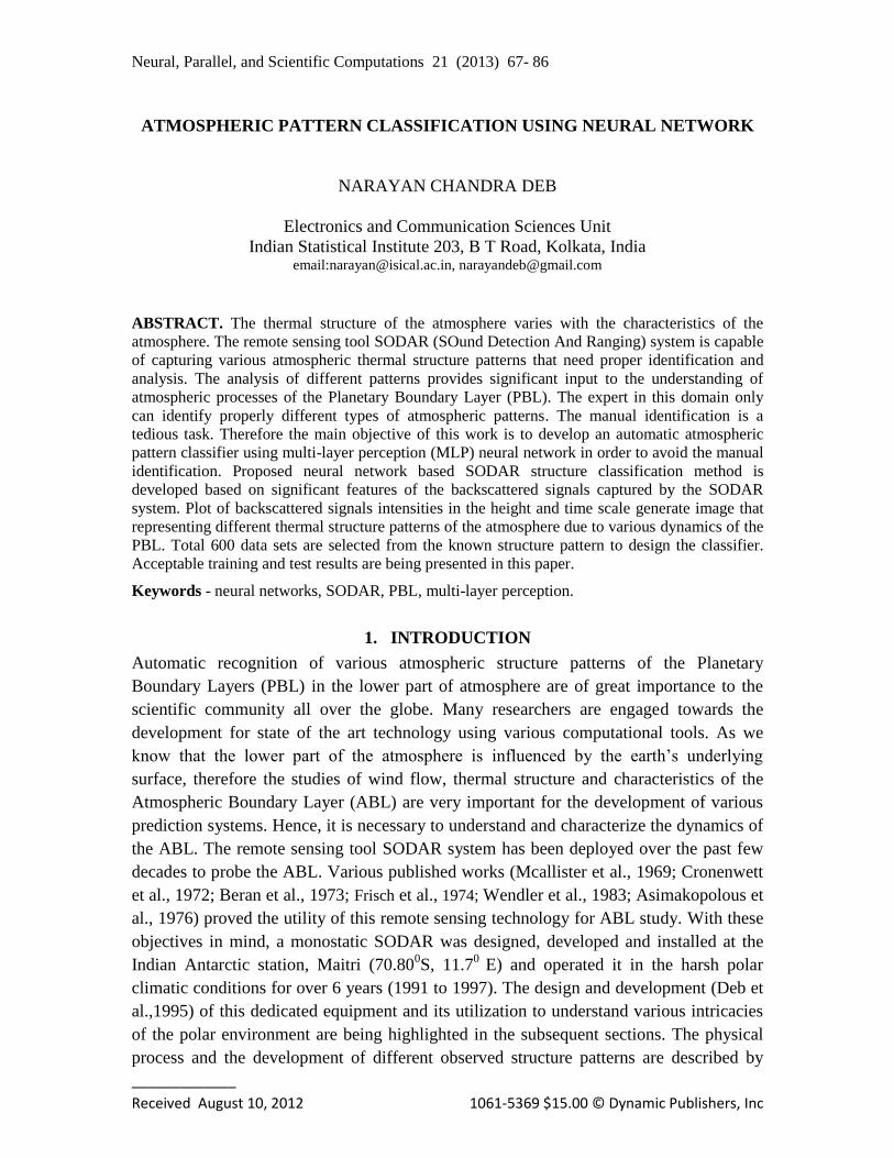
Figure 4: Structure pattern plotted from SODAR data for January 27, 1996

Then height, time and intensity of signals are plotted to generate image to view the

structure patterns. For each SODAR scan 400 intensity values are first converted its

equivalent gray value one by one using the expression , where 4096 is the

highest value of data, then plotted on the screen to obtain the image where ‘X’ axis is

treated as time scale and the ‘Y’ axis is treated as height scale as shown in Fig. 4. Various

types of SODAR structures are observed during (1991 – 1997) the operation of the

system. All these data were used for the Antarctic boundary layer study (Naithani et al.,

1994, 1995; Deb et al., 1999, 2001; Dutta et al., 1999; Gajananda et al., 2004; Kumar et

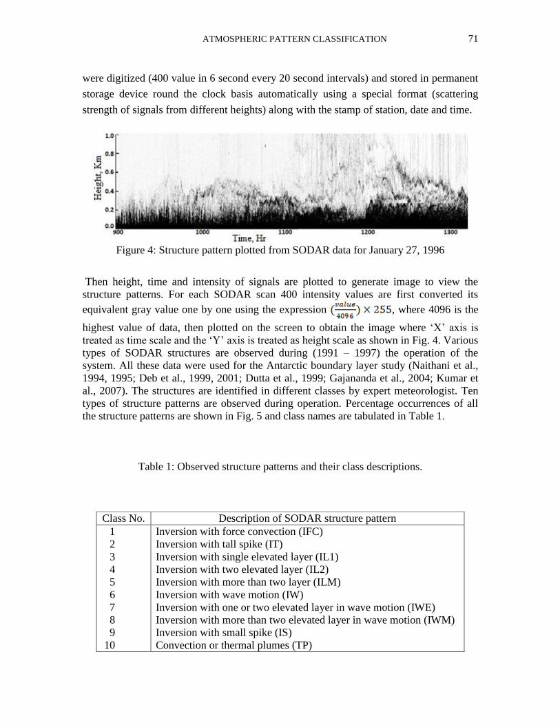
al., 2007). The structures are identified in different classes by expert meteorologist. Ten

types of structure patterns are observed during operation. Percentage occurrences of all

the structure patterns are shown in Fig. 5 and class names are tabulated in Table 1.

Table 1: Observed structure patterns and their class descriptions.

Class No. Description of SODAR structure pattern

1

2

3

4

5

6

7

8

9

10

Inversion with force convection (IFC)

Inversion with tall spike (IT)

Inversion with single elevated layer (IL1)

Inversion with two elevated layer (IL2)

Inversion with more than two layer (ILM)

Inversion with wave motion (IW)

Inversion with one or two elevated layer in wave motion (IWE)

Inversion with more than two elevated layer in wave motion (IWM)

Inversion with small spike (IS)

Convection or thermal plumes (TP)


Figure 5: Percentage occurrences of different structures as observed at Maitri,

Antarctica, during 1995-1997.

For this classification work we have considered only the class that appeared at site for at

least 2% or more occasions during observations recorded over a complete year. Fig. 5

shows three classes (IW, IWE, IWM) whose percentage occurrence < 2% and these three

classes are considered as a single class IEW on the basis of similar wave motion

characteristics. In this work, eight different structure patterns were selected using human

expert knowledge in this field. All these structure patterns were generated from the data

obtained by the system operated at Indian Antarctic base “Maitri” during 1995-1997. The

images of selected structure pattern classes are depicted in Figs. 6(a) – (h) and significant

property and relation with atmospheric process for the formation of all these classes are

described subsequently. From the graphical observation we have extracted each segment

(block of 400×180) for each class of structure from continuous data. Data are represented

as 3D image where X represents time, Y represents height, and intensity variation is third

dimension. From this pictorial representation of data various selected structures were

marked into different classes (Table 2) with the expert knowledge.

Table 2: Selected SODAR structure pattern classes.

3.3 Description of Atmospheric Pattern for Different Classes. All these eight selected

structure classes are representing a different thermodynamic state of the lower ABL.

From Table 2 it is evident that there are two main categories of structure inversion and

convection. Again among the inversion classes, there are 7 sub-classes.

Class No. Description of SODAR structure pattern

1

2

3

4

5

6

7

8

Inversion with force convection (IFC), Fig. 6(a)

Inversion with tall spike (IT), Fig. 6(b)

Inversion with single elevated layer (IL1), Fig. 6(c)

Inversion with two elevated layer (IL2), Fig. 6(d)

Inversion with more than two layer (ILM), Fig. 6(e)

Inversion with elevated layer in wave motion (IEW), Fig. 6(f)

Inversion with small spike (IS), Fig. 6(g)

Convection or thermal plumes (TP), Fig. 6(h)


(a) (b)

(c) (d)

(e) (f)

(g) (h)

Figure 6: Eight different classes of SODAR structure (a) IFC, (b) IT, (c) IL1, (d) IL2, (e)

ILM, (f) IEW, (g) IS, and (h) TP.


Atmospheric inversion is a phenomenon where temperature increases with increasing

height in the atmosphere instead of the usual inverse relation of temperature with altitude.

Under certain conditions, the normal vertical temperature gradient is inverted such that

the air is colder near the surface of the earth. This can occur when, a warmer, less dense

air mass moves over a cooler, dense air mass. So temperature inversion occurs when the

air temperature increases with height above the earth's surface. The different types of

inversion occur in the vicinity of warm fronts. An inversion is also produced whenever

radiation from the surface of the earth exceeds the amount of radiation received from the

sun, which commonly occurs at night, or during the winter when the angle of the sun is

very low in the sky. In Antarctica, about 95% of the time, inversions were recorded.

Some inversions were weak and dissipated quickly while others hang for several days

depending on the weather pattern. It was possible to record these inversions only for

winds below 12 mtr/s and beyond this wind speed, noise masks all the received signals.

We are discussing briefly about all types of inversion structures.

IFC (Inversion with Force Convection): Convection or advection is the movement of

fluids, atmospheric air packets in this case. In case of forced convection, the fluid

movement is not usually affiliated to natural forces like buoyancy. Sometimes, in high

wind conditions, the temperature inversion layer may be associated with force

convection, as shown in Fig 6.(a).

IT (Inversion with Tall spike): The inversion layer shows tall spike like structures. Under

moderately high wind conditions, the temperature inversion layers formed are associated

with tall spikes, as seen on the top of the layer. Formation of a temperature inversion

layer with tall spikes is shown in Fig 6.(b).

IL1 (Inversion with single elevated Layer): If there is an elevated part of the atmosphere

on the top of the surface based inversion layer, then IL1 is said to occur. At times an

inversion layer may be associated with single elevated layer, as shown in Fig 6(c).

IL2 (Inversion with two elevated Layer): The temperature inversion layer may be

associated with two elevated layers, as observed in Fig. 6(d). This condition is

favourable to form two elevated stable inversion layers.

ILM (Inversion with more than two elevated Layer): Sometimes, under very light wind

conditions, the temperature inversion layer may be associated with more than two

elevated layers, as observed in Fig. 6(e).

IEW (Inversion with Elevated layer in Wave motion): Inversion with wave like

structured layer form under light wind conditions and this temperature inversion layer

may be associated with wave motion, as observed in Fig. 6(f).

IS (Inversion with Small spike): During low wind, clam condition and absence of solar

energy temperature inversion layer with small spike is generally developed which is

shown in Fig. 6(g).

TP (Thermal Plumes): Thermal Plumes or Convection happens because warm air is less

dense than the cold air around it, so it is lighter and rises or goes up in the atmosphere.


Evidence of convection happening is seen when the sky is clear without clouds. There is

a constant balancing act going on all the time in our atmosphere as moist, warm air goes

upward and cooler, denser air moves down. This result in the formation of structures

called thermal plumes. Figure 6(h) describes the formation of typical convective

boundary layer with thermal plumes. Plume structures were seen to appear on cloudless,

clear sunny weather. This class represents an unstable atmospheric condition, in which

the transfer of heat, momentum, and energy from the surface level to the higher level and

vice-versa takes place. This layer brings a drastic change in the thermodynamic state of

the ABL.

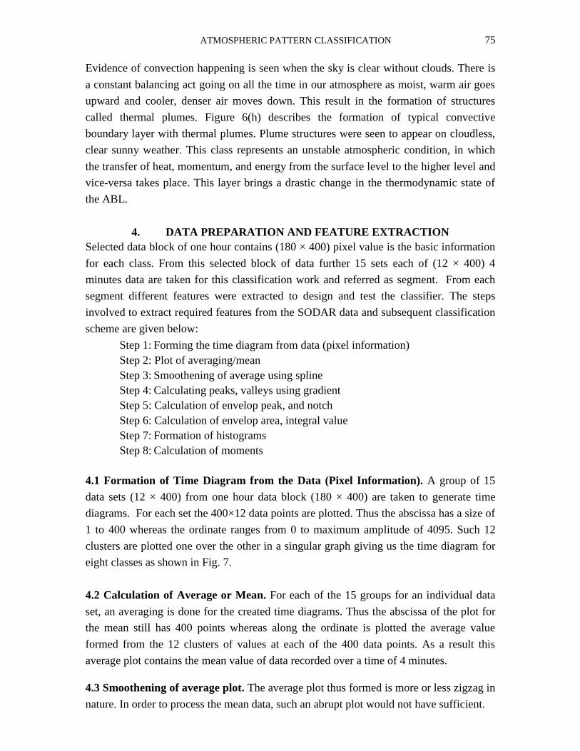
4. DATA PREPARATION AND FEATURE EXTRACTION

Selected data block of one hour contains (180 × 400) pixel value is the basic information

for each class. From this selected block of data further 15 sets each of (12 × 400) 4

minutes data are taken for this classification work and referred as segment. From each

segment different features were extracted to design and test the classifier. The steps

involved to extract required features from the SODAR data and subsequent classification

scheme are given below:

Step 1: Forming the time diagram from data (pixel information)

Step 2: Plot of averaging/mean

Step 3: Smoothening of average using spline

Step 4: Calculating peaks, valleys using gradient

Step 5: Calculation of envelop peak, and notch

Step 6: Calculation of envelop area, integral value

Step 7: Formation of histograms

Step 8: Calculation of moments

4.1 Formation of Time Diagram from the Data (Pixel Information). A group of 15

data sets (12 × 400) from one hour data block (180 × 400) are taken to generate time

diagrams. For each set the 400×12 data points are plotted. Thus the abscissa has a size of

1 to 400 whereas the ordinate ranges from 0 to maximum amplitude of 4095. Such 12

clusters are plotted one over the other in a singular graph giving us the time diagram for

eight classes as shown in Fig. 7.

4.2 Calculation of Average or Mean. For each of the 15 groups for an individual data

set, an averaging is done for the created time diagrams. Thus the abscissa of the plot for

the mean still has 400 points whereas along the ordinate is plotted the average value

formed from the 12 clusters of values at each of the 400 data points. As a result this

average plot contains the mean value of data recorded over a time of 4 minutes.

4.3 Smoothening of average plot. The average plot thus formed is more or less zigzag in

nature. In order to process the mean data, such an abrupt plot would not have sufficient.


Therefore in order to get a smoother version of the plot we resort to cubic spline method.

A smoother plot is thus obtained allowing us to proceed with finding the gradient of the

above mentioned plot. This has been done by selecting around 25-30 data points at

regular intervals from the mean plot and then plotting them by interpolating the abscissa

back to a domain of 400 points.

(a) (b)

(c) (d)

(e) (f)

(g) (h)

Figure 7: Time diagrams for eight classes (a) IFC, (b) IT, (c) IL1, (d) IL2, (e) ILM, (f)

IEW, (g) IS, and (h) TP.


4.4 Calculation of peaks and valleys using gradient. The gradient has been calculated

from the smoothened plot of the average diagram. The calculation of gradient has been

done in a linear manner by dividing the difference of alternate data points of the

interpolated function by the difference of the abscissa points. The peak and valley points

of the curves are determined by setting a threshold over the curve of the gradient. For all

the data classes a positive threshold value of +16 and a negative threshold value of –16

are set. The main logic for the determination of peaks and valleys is that as the gradient

curve is gradually traced along the abscissa when the curve starting from a point below

the negative threshold crosses the zero position and then extends over the positive

threshold, then the point on the smoothened average plot corresponding to this point on

the gradient plot is marked as a peak. Similarly for locating a valley, it is found that

points starting from above the positive threshold and abruptly falling below the negative

threshold correspond to the valleys, which are also similarly marked. The number of

peaks and valleys information acquired from the different data sets. Figure 7 shows time

diagram which represents average plot, spline as well as gradient for each data classes in

support of entire description.

4.5 Calculation of Envelope Peak and Notch.

Envelope Peak (enpk): The peak property considers the number of peaks of the

smoothed average time diagram. Here we have considered the number of peaks of the

smooth envelope of the time diagram. Here also the sliding procedure has been applied.

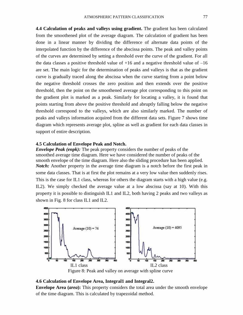
Notch: Another property in the average time diagram is a notch before the first peak in

some data classes. That is at first the plot remains at a very low value then suddenly rises.

This is the case for IL1 class, whereas for others the diagram starts with a high value (e.g.

IL2). We simply checked the average value at a low abscissa (say at 10). With this

property it is possible to distinguish IL1 and IL2, both having 2 peaks and two valleys as

shown in Fig. 8 for class IL1 and IL2.

IL1 class IL2 class

Figure 8: Peak and valley on average with spline curve

4.6 Calculation of Envelope Area, Integral1 and Integral2.

Envelope Area (area): This property considers the total area under the smooth envelope

of the time diagram. This is calculated by trapezoidal method.


Integral1 (int1) and Integral2 (int2): These two properties are helpful to determine the

width of the first peak of the smoothed average time diagram. For this, two equal

intervals on the time axis of the time diagram, each of duration 120 points (i.e., from 1 to

120 and from 121 to 240) are considered. Then the fractional areas under the curve (the

smooth averaged time diagram) are calculated in those two intervals. Now for a wide

peak it’s found that integral1 (area in the first interval) is around 0.7, i.e., around 70% of

the total area and integral2 (area in the second interval) is around 0.25, i.e., around 25%.

This is the case for classes having a wide peak (like IT) or classes having multiple peaks

distributed throughout the time axis of the time diagram (like ILM, IEW) or classes

having a single peak which is flat (IFC). Whereas for classes having a single narrow peak

(IS) or having two peaks that are situated near the origin of the time axis (IL1 and IL2)

the value of integral1 is higher, around 0.9 (i.e., around 90% of total area under the time

diagram) and value of integral2 is much lower; around 0.09 (i.e.,9% of the total area).

Values of integral1 (int1) and integral2 (int2) are calculated for each class.

4.7 Formation of Histograms. Histograms are plotted from the image intensity (range 0

to 255) of each class. Then frequency or number of occurrence for each intensity value is

calculated and then normalised so that the frequency values lie within 0 and 1. Then these

normalised frequencies are plotted in the form of bar diagram as shown in Fig. 9.

(a) (b) (c)

(d) (e) (f)

(g) (h)

Figure 9: Histogram of different classes (a) IFC, (b) IT, (c) IL1, (d) IL2, (e) ILM, (f)

IEW, (g) IS, and (h) TP.


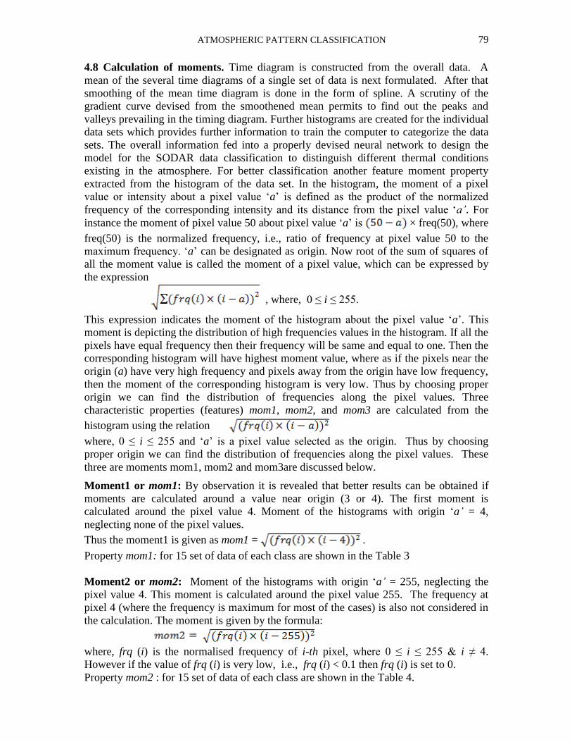
4.8 Calculation of moments. Time diagram is constructed from the overall data. A

mean of the several time diagrams of a single set of data is next formulated. After that

smoothing of the mean time diagram is done in the form of spline. A scrutiny of the

gradient curve devised from the smoothened mean permits to find out the peaks and

valleys prevailing in the timing diagram. Further histograms are created for the individual

data sets which provides further information to train the computer to categorize the data

sets. The overall information fed into a properly devised neural network to design the

model for the SODAR data classification to distinguish different thermal conditions

existing in the atmosphere. For better classification another feature moment property

extracted from the histogram of the data set. In the histogram, the moment of a pixel

value or intensity about a pixel value ‘a’ is defined as the product of the normalized

frequency of the corresponding intensity and its distance from the pixel value ‘a’. For

instance the moment of pixel value 50 about pixel value ‘a’ is × freq(50), where

freq(50) is the normalized frequency, i.e., ratio of frequency at pixel value 50 to the

maximum frequency. ‘a’ can be designated as origin. Now root of the sum of squares of

all the moment value is called the moment of a pixel value, which can be expressed by

the expression

, where, 0 ≤ i ≤ 255.

This expression indicates the moment of the histogram about the pixel value ‘a’. This

moment is depicting the distribution of high frequencies values in the histogram. If all the

pixels have equal frequency then their frequency will be same and equal to one. Then the

corresponding histogram will have highest moment value, where as if the pixels near the

origin (a) have very high frequency and pixels away from the origin have low frequency,

then the moment of the corresponding histogram is very low. Thus by choosing proper

origin we can find the distribution of frequencies along the pixel values. Three

characteristic properties (features) mom1, mom2, and mom3 are calculated from the

histogram using the relation

where, 0 ≤ i ≤ 255 and ‘a’ is a pixel value selected as the origin. Thus by choosing

proper origin we can find the distribution of frequencies along the pixel values. These

three are moments mom1, mom2 and mom3are discussed below.

Moment1 or mom1: By observation it is revealed that better results can be obtained if

moments are calculated around a value near origin (3 or 4). The first moment is

calculated around the pixel value 4. Moment of the histograms with origin ‘a’ = 4,

neglecting none of the pixel values.

Thus the moment1 is given as mom1 = .

Property mom1: for 15 set of data of each class are shown in the Table 3

Moment2 or mom2: Moment of the histograms with origin ‘a’ = 255, neglecting the

pixel value 4. This moment is calculated around the pixel value 255. The frequency at

pixel 4 (where the frequency is maximum for most of the cases) is also not considered in

the calculation. The moment is given by the formula:

where, frq (i) is the normalised frequency of i-th pixel, where 0 ≤ i ≤ 255 & i ≠ 4.

However if the value of frq (i) is very low, i.e., frq (i) < 0.1 then frq (i) is set to 0.

Property mom2 : for 15 set of data of each class are shown in the Table 4.


Table 3: Properties of mom1 calculated from 15 data sets for each class

Dataset IFC IT IL1 IL2 ILM IEW IS TP

1 200.627 187.1682 253.171 57.303 253.2971 251.1372 147.797 2.1873

2 181.9152 187.5192 236.069 72.3605 254.4288 251.1388 137.3852 2.1406

3 212.6666 205.0207 254.4861 73.9646 252.382 251.03 158.8864 1.8505

4 253.8311 221.2805 254.6783 73.6677 252.3153 252.3113 143.3309 1.7793

5 254.605 205.2562 253.0337 70.9728 254.2145 253.7515 137.2602 2.5154

6 236.6449 190.8994 251.444 71.5256 255.228 252.5582 153.7046 53.9906

7 255.2277 183.9757 252.8994 85.2503 255.3426 251.015 134.9069 2.1693

8 229.6747 195.7422 254.8501 92.5031 254.961 251.2877 174.5302 2.2378

9 256.8657 176.204 251.8587 80.6994 255.2786 252.8044 130.1177 53.99

10 254.4648 170.8328 253.6656 83.3804 255.7131 228.1985 118.4336 1.931

11 255.2276 189.3008 254.6451 83.4151 254.2339 254.2976 145.388 3.013

12 253.8408 179.164 255.0891 87.1289 255.8725 158.8664 114.7713 55.1444

13 237.3543 185.4862 255.1799 83.9154 256.3313 137.7672 135.6846 52.3753

14 254.1546 191.3491 256.799 90.1087 255.8508 145.8815 95.2287 66.6693

15 251.9891 192.5122 232.5609 94.6438 255.7497 145.9685 113.6127 65.9072

Range 182 - 257 171 - 221 232 - 256 57 - 94 252 - 256 137 - 254 95 - 159 1.8 - 67

Table 4: Properties of mom2 calculated from 15 data sets for each class


1 188.7569 87.1261 296.9469 148.4184 272.9416 222.7958 281.7648 135.0646

2 127.5579 103.1107 326.5689 119.4098 279.3822 223.698 267.0637 132.184

3 208.99 74.5837 248.2096 122.5426 283.8652 172.801 283.4711 114.2678

4 273.6995 103.3282 310.0982 112.1476 298.8288 182.4343 273.4535 109.8724

5 290.4878 99.1891 284.2479 110.4015 287.1984 225.4868 223.8192 155.3274

6 196.8338 67.327 246.1457 123.1892 292.4867 218.3203 266.2934 116.2702

7 191.1551 79.7913 241.9491 126.4405 257.9043 169.5943 266.1704 133.9537

8 243.4249 83.6711 307.6582 125.6575 277.0027 248.7162 314.5736 138.1835

9 254.5623 76.6452 259.7935 125.1006 260.2925 259.6073 264.8554 137.5589

10 232.5556 97.6545 243.7822 144.9138 257.4418 197.7819 263.3741 119.2414

11 242.5478 95.669 310.2965 135.0275 228.8214 308.8634 271.4879 186.0519

12 215.3991 68.1082 315.8189 143.4041 212.2447 185.3569 223.0354 106.5288

13 218.1794 64.4727 299.0734 158.516 247.2406 191.1066 275.4922 131.487

14 273.0989 86.2966 330.5897 172.8111 251.6459 195.84 231.0088 117

15 302.6373 89.359 354.5304 168.5485 237.3094 242.3318 343.0767 145.1469

Range 127-303 64-103 241-355 110-172 212-299 172-309 223-343 106-186

Moment3 or mom3: Moment of the histograms with origin ‘a’ = 4, Neglecting the pixel

value 255. This moment is calculated from the following formula:

where, frq(i) is the normalised frequency of i-th pixel value, 0 ≤ i ≤ 254. In this case we

have not considered the frequency of the pixel value 255. This eliminates the effect of the

high frequency value of pixel 255 and gives more insight about the histogram pattern.

Property mom3 : for 15 set of data of each class are shown in the Table 5.


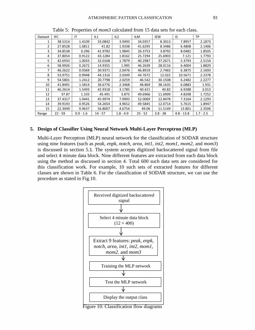
Table 5: Properties of mom3 calculated from 15 data sets for each class.


1 38.5314 1.4109 33.0842 3.9493 34.0357 8.3013 7.8957 2.1873

2 27.8528 1.0811 41.82 1.9338 41.6295 8.3486 6.4808 2.1406

3 34.8538 0.296 41.9782 1.9845 26.3753 3.8792 8.0482 1.8505

4 37.8054 0.9122 43.1284 1.8162 25.7294 25.6903 7.121 1.7793

5 42.6933 1.0033 32.0168 1.7879 40.2987 37.2671 5.3793 2.5154

6 58.9926 0.2672 14.9355 1.995 46.2639 28.0116 6.4004 1.8829

7 46.2622 0.9369 30.9371 2.0476 46.8919 2.7465 6.3875 2.1693

8 53.9751 0.9948 44.1316 2.0349 44.7672 12.022 10.5671 2.2378

9 54.5801 1.2412 20.7798 2.0259 46.542 30.1508 6.2482 2.2277

10 41.8491 1.5814 36.6776 2.3468 48.869 38.1635 6.0883 1.931

11 46.2614 1.5493 42.9318 3.1785 40.421 40.82 6.9288 3.013

12 37.87 1.103 45.491 3.875 49.6966 11.6909 4.8208 1.7252

13 37.4317 1.0441 45.9974 7.0993 52.0069 12.8478 7.3164 2.1293

14 39.9193 0.9526 54.2654 4.9652 49.5845 12.0714 5.7615 1.8947

15 22.3049 0.9637 56.8007 4.6754 49.06 11.5149 13.801 2.3506

Range 22 - 59 0.9 - 1.6 14 - 57 1.8 - 4.9 25 - 52 3.8 - 38 4.8 - 13.8 1.7 - 2.5

5. Design of Classifier Using Neural Network Multi-Layer Perceptron (MLP)

Multi-Layer Perceptron (MLP) neural network for the classification of SODAR structure

using nine features (such as peak, enpk, notch, area, int1, int2, mom1, mom2, and mom3)

is discussed in section 5.1. The system accepts digitized backscattered signal from file

and select 4 minute data block. Nine different features are extracted from each data block

using the method as discussed in section 4. Total 600 such data sets are considered for

this classification work. For example, 10 such sets of extracted features for different

classes are shown in Table 6. For the classification of SODAR structure, we can use the

procedure as stated in Fig.10.

Figure 10: Classification flow diagrams

Received digitized backscattered

signal

Select 4 minute data block

(12 × 400)

Extract 9 features: peak, enpk,

notch, area, int1, int2, mom1,

mom2, and mom3

Training the MLP network

Display the output class

Test the MLP network


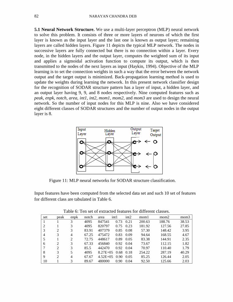
5.1 Neural Network Structure. We use a multi-layer perceptron (MLP) neural network

to solve this problem. It consists of three or more layers of neurons of which the first

layer is known as the input layer and the last one is known as output layer; remaining

layers are called hidden layers. Figure 11 depicts the typical MLP network. The nodes in

successive layers are fully connected but there is no connection within a layer. Every

node, in the hidden layers and the output layer, computes the weighted sum of its input

and applies a sigmoidal activation function to compute its output, which is then

transmitted to the nodes of the next layers as input (Haykin, 1994). Objective of the MLP

learning is to set the connection weights in such a way that the error between the network

output and the target output is minimized. Back-propagation learning method is used to

update the weights during learning the network. In this present network classifier design

for the recognition of SODAR structure pattern has a layer of input, a hidden layer, and

an output layer having 9, 9, and 8 nodes respectively. Nine computed features such as

peak, enpk, notch, area, int1, int2, mom1, mom2, and mom3 are used to design the neural

network. So the number of input nodes for this MLP is nine. Also we have considered

eight different classes of SODAR structures and the number of output nodes in the output

layer is 8.

Figure 11: MLP neural networks for SODAR structure classification.

Input features have been computed from the selected data set and such 10 set of features

for different class are tabulated in Table 6.

Table 6: Ten set of extracted features for different classes.

set peak enpk notch area int1 int2 mom1 mom2 mom3

1 1 3 4095 847541 0.73 0.21 200.63 188.76 38.53

2 1 3 4095 820797 0.75 0.23 181.92 127.56 27.85

3 2 3 83.91 407379 0.85 0.08 57.30 148.42 3.95

4 3 4 67.25 475472 0.83 0.09 94.64 168.55 4.67

5 1 2 72.75 448617 0.89 0.05 83.38 144.91 2.35

6 2 3 67.33 456840 0.92 0.04 73.67 112.15 1.82

7 2 3 85.5 442470 0.92 0.04 70.97 110.40 1.79

8 3 5 4095 8.27E+05 0.68 0.18 254.22 287.19 40.29

9 2 4 67.67 4.52E+05 0.90 0.05 85.25 126.44 2.05

10 1 3 89.67 480000 0.90 0.04 92.50 125.66 2.03


We have prepared the data file with 9 + 8 = 17 fields in a record of which 9 computed

features as input and remaining 8 fields are output which indicate either presence by ‘1’

or absence by ‘0’. That means in a record one of these eight output fields is one and

remaining are zeros. These eight classes are defined in Table 7

Table 7: The arrangement of various classes in the output string

1 2 3 4 5 6 7 8

IFC IT IL1 IL2 ILM IEW IS TP

5.2 Training and Test the Network. Initially, we mix the data set randomly. Then we

partitioned the data into two parts, one part contains 80% of data used as training the

model and the remaining 20% of these data used as test the performance of the trained

model. This neural network (MLP) is trained with different hidden nodes such as 5, 6, 7,

8, 9, 10, 15, 20, 25, 30 up-to different levels of iterations from 300 to 1200. The

performance of the model is tabulated in Tables 8 and 9.

Table 8: Percentage recognition score with training data set for different hidden node No. of Iteration

For different hidden node (H)

H = 5 H = 6 H = 7 H = 8 H = 9 H = 10 H = 15 H = 20 H = 25 H = 30

300 73.778 82.667 84.444 89.556 88.667 86.444 92.444 93.778 94.222 93.333

400 74.444 81.333 86.667 86.889 90.667 89.111 94.667 97.778 92.889 94.000

500 76.222 84.222 84.667 88.000 89.556 92.000 96.444 95.111 96.667 95.111

600 79.778 82.889 86.667 90.000 91.111 91.556 96.889 96.222 98.222 96.889

700 74.000 82.889 86.000 88.222 91.333 91.333 96.667 97.111 96.444 96.667

800 78.889 85.556 85.778 90.889 90.444 91.556 94.889 98.000 95.556 97.111

900 78.667 82.222 87.333 88.889 92.444 91.556 96.000 97.556 97.778 98.222

1000 77.778 84.667 90.000 90.222 93.556 92.889 97.333 96.222 98.000 98.444

1100 75.778 83.778 87.556 90.222 90.667 92.000 96.222 98.667 97.556 98.000

1200 76.889 84.667 87.556 88.444 91.111 93.556 96.222 99.111 98.667 98.222

Table 9: Percentage recognition score with test data set for different hidden node

6. Results and Conclusions

The neural network model (MLP) is designed for identification of atmospheric structures

generated by a SODAR system using the knowledge, experiences and expertise of the

No. of Iteration

For different hidden node (H)

5 6 7 8 9 10 15 20 25 30

300 70.667 77.333 76.667 76.667 79.333 84.000 86.667 90.810 88.000 88.000

400 70.000 73.333 78.000 82.667 84.000 84.667 88.667 87.333 89.333 88.000

500 70.667 77.333 78.667 79.333 82.000 84.000 86.667 88.667 88.667 90.000

600 74.667 76.667 81.333 80.000 86.000 84.000 83.333 84.667 89.333 86.000

700 70.000 78.000 77.333 77.333 83.333 87.333 88.000 91.333 87.333 89.333

800 70.667 76.667 80.667 76.000 86.000 83.333 86.000 88.000 88.000 88.000

900 72.667 72.000 78.667 80.000 86.000 83.333 87.333 85.333 90.000 89.333

1000 71.333 80.667 81.333 80.667 87.333 87.333 85.333 89.333 90.667 91.333

1100 69.333 79.333 77.333 83.333 84.000 87.333 89.333 88.667 90.000 89.333

1200 72.000 79.333 78.667 83.333 84.000 82.000 85.333 90.000 88.000 90.000


human expert working in this field. Table 8 and Table 9 depict the result of the

performance of the present model of atmospheric structure classification. All eight

classes are correctly classified in terms of accuracy. The Table 8 shows that 97.1%

recognition score achieved for training set data, when model runs for 700 iterations with

20 hidden nodes, and 91.33% recognition score achieved for test set data, when model

runs for 700 iterations with 20 hidden nodes as indicated in Table 9. Thus we have

achieved successful classification of SODAR data.

The SODAR system has emerged as a useful remote sensing tool that provides

information about the formation of different types of thermal structures like temperature

inversion, thermal plumes, elevated multilayered inversion, fog layers, and other various

types of PBL (Planetary Boundary Layer) structures, at low cost and continuous basis. It

was evident that SODAR signatures were representing various structures believed to be

associated with the formation and changes in the PBL characteristics. We designed

classifier in the soft-computing paradigm can automatically recognize the PBL structures

in order to avoid the tedious job of manual identification of the different types of useful

SODAR patterns. We have used neural network architecture to classify eight different

types of SODAR patterns and this may be one of the solutions of the SODAR pattern

classification problems. Multi-layer perceptron (MLP) neural network models are

inherently suitable in data-rich environments and extract underlying relationships from

the data domain. The classifier reduces dependence on human experts for the

identification of SODAR structure patterns. The results obtained by testing the model are

satisfactory. This classifier tool may be applicable for both offline and online SODAR

structure recognition. With this enhancement, we can develop a new SODAR system

incorporating automatic structure classification scheme for different applications. Finally,

this study holds promise for researchers working in the domains of atmospheric sciences,

remote sensing, air pollution, meteorology, and civil aviation.

REFERENCES

1. Mcallister, L.G., Pollard, J.R.,Mahohey, A.R. & Shaw, P.J.R., (1969), Acoustic

sounding – a new approach to the study of atmospheric structure. Proceedings of

IEEE, v. 57, pp. 579–587.

2. Cronenwett, W.T., Walker, G.B. & Inman, R.L., (1972), Acoustic sounding of

meteorological phenomena in the planetary boundary layer. Journal of Applied

Meteorology, v. 11, pp. 1351–1358.

3. Beran, D.W., Hooke, W.H. & Clifford, S.F., (1973), Acoustic echo-sounding

techniques and their application to gravity wave, turbulence and stability studies.

Earth and Environmental Science, v. 4, pp. 133–153.


4. Frisch, A.S., & Clifford, S.F., (1974), A study of convection capped by a stable

layer using Doppler radar and acoustic echo sounder, Journal of Applied


5. Wendler , G., Kodama, Y., & Poggi, A., (1983), Katabatic winds in Adelie Land,

Antarctic Journal of United States, v. 18, pp. 236- 238.

6. Asimakopolous, D.N., Cole, R.S., Caughey, S.J. & Crease, B. A., (1976), A

quantitative comparison between acoustic sounder returns and the direct

measurement of atmospheric temperature fluctuations. Boundary Layer


7. Deb, N. C., Naithani, J., & Kapoor, M., (1995), Design and Development of a PC

controlled Acoustic Sounding System for Antarctica, Eleventh Indian Expedition

to Antarctica, Scientific Report, Depertment of Ocean Development, Technical

Publication No.9, pp. 79-86.

8. Deb, N.C., Pal, S., Patranabis, D. C., & Dutta, H. N., (2010), A neurocomputing

model for sodar structure classification, International Journal of Remote Sensing, v.

31, 2995 – 3018.

9. Deb, N.C., Ray, K. S., & Dutta, H. N., (2011), SODAR Pattern Classification by

Graph Matching, IEEE Geosciences and Remote Sensing Letters, v. 8, pp 483-487.

10. Kalogiros, J.A., Helmis, C.G., Asimakopoulos, D.N., Papageorgas, P.G. &

Soilemes, A.T., (1995), A layer detection and classification algorithm for sodar

facsimile records. International Journal of Remote Sensing, v. 16, pp. 2939–2954.

11. Mukherjee, A., Pal, P. & Das, J., (2002), Classification of sodar data using fractal

features. Poster presentation at Proceedings of Indian Conference on Computer

Vision, Graphics & Image Processing, 16–18 December, Ahmedabad, India, pp.

203-207.

12. Choudhury, S. & Mitra, S., (2004), A connectionist approach to SODAR pattern

classification. IEEE Geosciences and Remote Sensing Letters, v. 1, pp. 42–46.

13. Chaudhuri, B.B., De, A.K., Gnaguly A. & Das, J., (1992), Automatic recognition

and Interprtation of sodar records. Indian Journal of Radio Space Physics, v. 21, pp.

123–128.

14. Mukherjee, A., Pal, P. & Das, J., (1999), Identification of elementary sodar patterns

using perceptrons. In Proceedings of fourth International Conference on advance in

pattern recognition and digital techniques, December 1999, India. (New Delhi,

India:Narosa) pp. 83-86.

15. Koul, P. N., (1995), A Report on the Operations Carried Out By Survey of India

Team During Eleventh Indian Expedition to Antarctica; Eleventh Indian Expedition

to Antarctica, Scientific Report, Department of Ocean Development, Technical

Publication No.9, pp. 145-151.


16. Naithani, J., Dutta, H. N., Pasricha, P. K., Reddy, B. M., & Aggarwal, K. M.,

(1994), Evaluation of heat and momentum fluxes over Maitri, Antarctica,

Boundary Layer meteorology, v. 74, pp.195-208.

17. Naithani, J., & Dutta, H. N., (1995), Acoustic sounder measurements of the

planetary boundary layer at Maitri, Antarctica, Boundary layer Meteorology, v. 76,

pp. 199-207.

18. Deb, N. C., Srivastava, M. K., Singh, R., Pasricha, P. K., & Dutta, H. N., (1999),

Warm spell over Schirmacher region of east Antarctica during February, 1996,

DOD Tech Pub No. 13, pp. 71-78.

19. Deb, N. C., Chowdhury, S., & Pal, A., (2001), Acoustic Remote Sensing of LPBL

over Antarctica,” Indian Journal of Physics, v. 75B, pp. 259-262.

20. Dutta, H. N., Srivastava, M. K., Pasricha, P. K., Gajananda, Kh., Naithani, J.,

Deb, N. C., Ojha, D., & Gupta, V. B., (1999), Cyclone induced warming over a

wide spread region in east Antarctica : a case study, NPL Report No. DOD/12-

MMDP/8-97-MRC Cell/01, NPL, New Delhi, October, pp. 1-15.

21. Gajananda, Kh., Kaushik, A., & Dutta, H. N., (2004), Thermal convection over

east Antarctica: Potential microorganism dispersal, International Journal of

Aerobiologia v. 20, pp. 21-34.

22. Kumar, A., Gupta, V. B., Dutta, H. N., & Ghude, S., (2007), Mathematical

modelling of katabatic winds over Schirmacher region, East Antarctica, Indian J

Radio & Space Phys., v. 36, pp. 204-212.

23. Haykin, S., (1994), Neural Networks: A Comprehensive Foundation, New York:

Macmillan.

atmospheric pattern classification using neural …

Documents