Atmospheric Circulation of Extrasolar Planets

Adam P. ShowmanUniversity of Arizona

James Y-K. ChoQueen Mary, University of London

Kristen MenouColumbia University

We survey the basic principles of atmospheric dynamics relevant to explaining existingand future observations of extrasolar planets, both gas giant and terrestrial. Given the paucityof data on extrasolar planet (or “exoplanet”) atmospheres,our approach is to emphasizefundamental principles and insights gained from Solar System studies that are likely to begeneralizable to exoplanets. We begin by presenting the hierarchy of some basic equations setsused in atmospheric dynamics, including the Navier-Stokes, primitive, equivalent-barotropic,shallow-water, and two-dimensional nondivergent models.We then survey key concepts inatmospheric dynamics, including the importance of planetary rotation, the concept of balance,and simple scaling arguments to show how turbulent interactions generally produce large-scaleeast-west banding on rotating planets. We next turn to issues specific to giant planets, includingtheir expected interior and atmospheric thermal structures, the implications for their windpatterns, and mechanisms to pump their east-west jets. Hot Jupiter atmospheric dynamicsare given particular attention, as these close-in planets have been the subject of most of theconcrete developments in exoplanetary atmospheres. We then turn to the basic elements ofcirculation on terrestrial planets as inferred from Solar System studies, including Hadleycells, jet streams, processes that govern the large-scale horizontal temperature differences, andclimate, and we discuss how these insights may apply to extrasolar terrestrial planets. Althoughexoplanets surely possess a greater diversity of circulation regimes than seen on the planets inour Solar System, our guiding philosophy is that the multi-decade study of Solar System planetsreviewed here provides a foundation upon which our understanding of more exotic exoplanetarymeteorology must build.

1. INTRODUCTION

Since the first discovery of extrasolar giant planetsaround Sun-like stars via Doppler velocimetry (Mayor andQueloz 1995; Marcy and Butler 1996), extrasolar planetresearch has experienced a spectacular series of observa-tional breakthroughs. The first discovery of a transitinghot Jupiter1 (Charbonneau et al. 2000; Henry et al. 2000)opened the door to a wide range of clever techniques forcharacterizing such transiting planets. The drop in flux thatoccurs during secondary eclipse, when the planet passes be-hind its star, led to direct infrared detections of the thermalflux from the planet’s dayside (Deming et al. 2005; Char-bonneau et al. 2005). This was quickly followed by thedetection of day/night temperature variations (Harringtonet al. 2006), detailed phase curve observations (e.g. Knut-son et al. 2007, 2009; Cowan et al. 2007), infrared spec-tral and photometric measurements (Grillmair et al. 2007,

1The terms hot Jupiter and hot Neptune refer to extrasolar giant planetswith masses comparable to those of Jupiter and Neptune, respectively, withorbital semi-major axes less than∼ 0.1 AU, leading to high temperatures.

2008; Richardson et al. 2007; Charbonneau et al. 2008;Knutson et al. 2008a) and a variety of transit spectroscopicconstraints (Tinetti et al. 2007; Swain et al. 2008; Barman2008). Collectively, these observations help to constrainthe composition, albedo, three-dimensional (3D) tempera-ture structure, and hence the atmospheric circulation regimeof hot Jupiters.

Additional photometric and spectroscopic constraints onthe atmospheres of hot Jupiters and hot Neptunes will be-come available in the next few years, with repeated eclipsemeasurements, multi-wavelength infrared (IR) coverage,densely sampled phase curves and improved infrared andtransit spectra. Similar observational constraints on po-tentially habitable Earth-like planets around nearby M-dwarf stars may even be within our reach over the nextdecade (Charbonneau and Deming 2007). These rapidobservational developments imply that the physical con-ditions present in the distant atmospheres of hot Jupitersand Neptunes (and eventually warm Earths) can be directlyconstrained by remote astronomical observing. The muchincreased infrared sensitivity of the upcomingJames Webb

1

Space Telescoperelative to the currentSpitzer Space Tele-scopeguarantees that transiting/eclipsing systems will re-main powerful astronomical tools for the study of nearbyexoplanetary atmospheres in the future (Seager et al. 2008).

Transiting systems also provide constraints on key plan-etary attributes; these constraints are a prerequisite to char-acterizing the atmospheric circulation regimes of the plan-ets. When combined with Doppler velocimetry data, transitobservations permit a direct measurement of the exoplanet’sradius, mass and thus surface gravity2. With the additionalexpectation that close-in exoplanets are tidally locked ifona circular orbit, or pseudo-synchronized3 if on an eccentricorbit, the planetary rotation rate is thus indirectly knownaswell. Knowledge of the radius, surface gravity, rotation rateand external irradiation conditions for several exoplanets,together with the availability of direct observational con-straints on their emission, absorption and reflection prop-erties, opens the way for the development of comparativeatmospheric science beyond the reach of our own Solar Sys-tem.

The need to interpret these astronomical data reliably,by accounting for the effects of atmospheric circulation andunderstanding its consequences for the resulting planetaryemission, absorption and reflection properties, is the centraltheme of this chapter. Tidally locked close-in exoplanetsare subject to an unusual situation of permanent day/nightradiative forcing, which does not exist in our Solar System4.To address the new regimes of forcings and responses ofthese exoplanetary atmospheres, a discussion of fundamen-tal principles of atmospheric fluid dynamics and how theyare implemented in multi-dimensional, coupled radiation-hydrodynamics numerical models of the GCM (GeneralCirculation Model) type is required.

Contemplating the wide diversity of exoplanets raisesa number of fundamental questions. What determines themean wind speeds, direction, and 3D flow geometry in at-mospheres? What controls the equator-to-pole and day-night temperature differences? What controls the frequen-cies and spatial scales of temporal variability? What roledoes the circulation play in controlling the mean climate(e.g., global-mean surface temperature, composition) of anatmosphere? How do these answers depend on parame-ters such as the planetary rotation rate, gravity, atmosphericmass and composition, and stellar flux? And, finally, whatare the implications for observations and habitability of ex-oplanets?

At present, only partial answers to these questions exist(see reviews by Showman et al. 2008b; Cho 2008). With up-coming observations of exoplanets, constraints from solar-system atmospheres, and careful theoretical work, signif-

2Combining Doppler velocimetry and transit measurements lifts the mass-inclination degeneracy.

3Pseudo-synchronization refers to a state of tidal synchronization achievedonly at periastron passage (=closest approach), as expected from the strongdependence of tides with orbital separation.

4Venus may provide a partial analogy, which has not been fullyexploitedyet.

icant progress is possible over the next decade. While arich variety of atmospheric flow behaviors is realized in theSolar System alone—and an even wider diversity is pos-sible on exoplanets—the fundamental physical principlesobeyed by all planetary atmospheres are nonetheless uni-versal. With this unifying notion in mind, this chapter pro-vides a basic description of atmospheric circulation princi-ples developed on the basis of extensive Solar System stud-ies and discusses the prospects for using these principles tobetter understand physical conditions in the atmospheres ofremote worlds.

2. EQUATIONS AND CONCEPTS GOVERNINGATMOSPHERIC CIRCULATION

2.1. Fundamental equations

Under a wide range of conditions, the atmosphere can beaptly described as a fluid, which we assume here to be elec-trically neutral. For a good understanding of atmosphericcirculation, a hierarchy of atmospheric fluid dynamics mod-els is required—along with a good understanding of theproperties of the individual model equation sets and the re-lationship between them. Reduced models, which excludecertain fast waves, give less complete descriptions of the at-mosphere. However, they can adequately describe the (usu-ally more important) slow motions and elucidate a numberof mechanisms not easily captured in the full model.

2.1.1. Navier-Stokes Equations

Let u = u(x, t) be velocity at positionx and timet,wherex,u ∈ R

3. If the frictional force per unit area of thefluid is linearly proportional to shear in the fluid, then it isa Newtonian fluid (e.g., Batchelor 1967). Such fluids aredescribed by the Navier-Stokes equations:

Du

Dt= −1

ρ∇p+ fb +

1

ρ∇·

2µ

[

e − 1

3(∇·u) I

]

, (1a)

where

D

Dt=

∂

∂t+ u·∇ (1b)

is the material derivative (i.e., the deriative following themotion of a fluid element). Here,ρ is density,p is pres-sure,fb represents various body forces per mass (e.g., grav-ity and Coriolis),µ is molecular dynamic viscosity, ande = 1

2[(∇u)+(∇u)T] andI are the strain-rate and unit ten-

sors, respectively. In Eq. (1a) the quantity inside the bracesis the viscous stress tensor. Here, as in Eq. (3) below, theaverage normal viscous stress (bulk viscosity) has been as-sumed to be zero.

Eq. (1a) is closed with the following equations for mass(per unit volume), internal energy (per unit mass), and state:

Dρ

Dt= −ρ∇·u, (2)

2

Dǫ

Dt= −p

ρ(∇ · u) +

2µ

ρ

[

e : (∇u)T − 1

3(∇ · u)2

]

+1

ρ∇ · (KT∇T ) + Q, (3)

p = p(ρ, T ), (4)

whereǫ = ǫ(T, s) is specific internal energy,s is specificentropy,KT is heat conduction coefficient,T is tempera-ture, andQ is thermodynamic heating rate per mass. InEq. (3) “ : ” is scalar-product (i.e., component-wise multi-plication) operator for two tensors. Eqs. (1–4) constitute6equations for 6 independent unknowns,u, p, ρ, T . Notethat for a homogeneous thermodynamic system, which in-volves a single phase, only two state variables can vary in-dependently; hence, there are only two thermodynamic de-grees of freedom for such a system.

The neutral atmosphere is well described by Eqs. (1–4)when the characteristic length scaleL is much larger thanthe mean free path of the constituents that make up the at-mosphere. Hence, the equations are valid up to heightswhere ionization is not significant and the continuum hy-pothesis does not break down. Under normal conditions,the atmosphere behaves like an ideal gas. The parametersµ, KT, and other physical properties of the fluid depend onT , as well asρ. When appreciable temperature differencesexists in the flow field, these properties must be regarded asa function of position. For large-scale atmosphere applica-tions, however, the terms involvingµ in Eqs. (1a) and (3)are small and can be neglected in most cases. The typicalboundary conditions areu · n = 0 at the lower boundary,wheren is the normal to the boundary, andρ, p → 0 asz → ∞. For local, limited area models, periodic boundaryconditions are often used.

2.1.2. The Primitive Equations

On the large scale (to be more precisely quantified be-low), the motion of an atmosphere is governed by the prim-itive equations. They read (e.g., Salby 1996):

Dv

Dt= −∇p Φ − fk×v + F −D (5a)

∂Φ

∂p= −1

ρ(5b)

∂

∂p= −∇p · v (5c)

Dθ

Dt=

θ

cpTqnet , (5d)

whereD

Dt=

∂

∂t+ v·∇p +

∂

∂p. (5e)

Note here thatp, rather than the geometric heightz, isused as the vertical coordinate. This coordinate, which sim-plifies the gradient term in Eq. (5a), is common in atmo-spheric studies; it rendersz = z(x, p, t) a dependent vari-able, where nowx ∈ R

2. In Eq. (5)v(x, t) = (u, v) is

the (eastward, northward) velocity in a frame rotating withΩ; Φ = gz is the geopotential, whereg is the gravitationalacceleration (assumed to be constant and to include the cen-trifugal acceleration contribution; see Holton 2004, pp. 13-14) andz is the height above a fiducial geopotential surface;k is the local upward unit vector;f = 2Ω sinφ is the Cori-olis parameter, the locally vertical component of the plan-etary vorticity vector2Ω; ∇p is the horizontal gradient ona p-surface; = Dp/Dt is the vertical velocity;F andD represent the momentum sources and sinks, respectively;θ = T (pref/p)

κ is the potential temperature5, wherepref is areference pressure andκ = R/cp with R the specific gasconstant andcp the specific heat at constant pressure; andqnet is thenetdiabatic heating rate (heating minus cooling).Note thatqnet can include not only radiative heating/coolingbut latent heating and, at low pressures where the thermalconductivity becomes large, conductive heating. The New-tonian cooling scheme, which relaxes temperature toward aprescribed radiative-equilibrium temperature over a speci-fied radiative time constant, is one simple parameterizationof qnet.

The fundamental presumption in the use of Eqs. (5) isthat small scale processes are parameterizable within theframework of large-scale dynamics. Here by “large” scales,it is meant typicallyL & a/10, wherea is the planetaryradius. By “small” scales, it is meant those scales thatare not resolvable numerically by global models—typically. a/10. Regions of the atmosphere where small scaleprocesses are important are often highly concentrated (e.g.,fronts and convective updrafts). Their characteristic scalesare≪a/10. Therefore, it is possible that the Eq. (5) set—aswith all the other equation sets discussed in this chapter—leaves out some processes important for large-scale dynam-ics, particularly over long timescales.

To arrive at Eq. (5), one begins with Eqs. (1–4) in spher-ical geometry (e.g., Batchelor 1967). Two approximationsare then made. These are the “shallow atmosphere” andthe “traditional” approximations (e.g., Salby (1996)). Thefirst assumesz/a ≪ 1. The second is formally validin the limit of strong stratification, when the Prandtl ra-tio (N2/Ω2) ≫ 1. Here,N = N(x, z, t) is the Brunt-Vaisala (buoyancy) frequency, the oscillation frequency foran air parcel that is displaced vertically under adiabatic con-ditions:

N =

[

g∂(ln θ)

∂z

]1/2

. (6)

These approximations allow the Coriolis terms involvingvertical velocity to be dropped from Eq. (1a) and verticalaccelerations to be assumed small. The latter is explicitlyembodied in Eq. (5b), the hydrostatic balance, which wediscuss further below.

Hydrostatic balance renders the primitive equations validonly whenN2/ω2 ≫ 1, where2π/ω is the timescale of the

5The potential temperatureθ is related to the entropys by ds = cpd ln θ.Whencp is constant, this yieldsθ = T (pref/p)

κ.

3

motion under consideration. This condition, which is dis-tinct from the Prandtl ratio condition, restricts the verticallength scale of motions to be small compared to the hori-zontal length scale. Therefore, the hydrostatic balance ap-proximation breaks down in weakly stratified regions (herewe refer to the dynamically evolving hydrostatic balance as-sociated with circulation-induced perturbations in pressureand density; the mean background density and pressure—i.e., those that would exist in absence of dynamics—willremain hydrostatically balanced even when the circulation-induced perturbations are not). The hydrostatic assumptionfilters vertically propagating sound waves from the equa-tions.

According to Eq. (5d), whenqnet = 0, individual valuesof θ are retained by fluid elements as they move with theflow. In this case, Eq. (5) also admit a dynamically impor-tant conserved quantity, the potential vorticity:

qPE =

[

(ζ + f)k

ρ

]

·∇θ, (7a)

whereζ = k · ∇×v is the relative vorticity. This quantityprovides the crucial connection between the primitive equa-tions and the physically simpler models that follow. For ex-ample, undulations of potential vorticity are often a directmanifestation of Rossby waves, which are represented inall the models presented in this and following subsections.The conservation of the potential vorticityqPE following theflow,

DqPE

Dt= 0 , (7b)

and the redistribution ofqPE implied by it, is one of the mostimportant properties in atmospheric dynamics.

2.1.3. One-Layer Models

For many applications, Eq. (5) is too complex and broadin scope. In the absence of observational information toproperly constrain the model parameters, reduction of theequations is beneficial. A commonly used approach is tocollapse the 3D primitive equations to a two-dimensional(2D), one-layer model. Such reduction allows investigationof horizontal vortex and jet interactions in an idealized set-ting. Here we discuss these models starting with the mostcomplex.

Equivalent-Barotropic Model

One useful reduction is the equivalent-barotropic equa-tions (Salby 1989), which are obtained by vertically inte-grating Eq. (5). The reduced equations govern the dynam-ics of a semi-infinite gas layer, which is bounded below bya material surface. The equation of state that applies in thelayer is p = p(ρ). The bounding surface at the bottomdeforms according to the local temperature on the surface.The equations read:

D〈v〉Dt

= −∇(H + HB ) − fk×〈v〉 + Dv (8a)

DHDt

= −κH∇·〈v〉 + DH , (8b)

where

D

Dt=

∂

∂t+ 〈v〉·∇. (8c)

In Eq. (8),〈v(x, t)〉 is the pressure-averaged velocity, inte-grated fromp0(x, t) to p = 0, and

H =θ0A0Γ

(

p0

pref

)κ

, (9)

with Γ the vertical gradient of temperature,HB = z0/A0,andDv andDH the forcing and dissipation for momen-tum and thickness, respectively. Here, the “0” subscriptrefers to the value of the variable at the bottom boundingsurface, which is generally a function ofx andt. For exam-ple,A0 = A(θ0) is the value of the equivalent-barotropicstructure functionA(θ(p)) andz0 = z0(x) is the prescribedelevation of the bounding surface.A itself is defined suchthat (Charney 1949)

v(x, p, t) = A(θ) 〈v(x, t)〉. (10)

For vertically aligned flows,A = 1, and is independent ofthe vertical coordinate. The boundary condition is then

Dθ0Dt

= 0 (11)

in the adiabatic case, sinceθ0 is uniform. In the diabaticcase, this equation with forcing terms becomes a formal ad-dition to the set of equivalent-barotropic equations.

Whenκ = 1, the set of Eq. (8) is formally identical tothe shallow-water equations with〈v〉 = (u, v) and bot-tom topography. Here,u andv have their usual meanings(cf., §2.1.2).

Equation (8) admit an important conservation law anal-ogous to Eq. (7). In the absence of heating and dissipation,the equivalent-barotropic potential vorticity,

qEB =〈ζ〉 + f

H1/κ(12)

is conserved following the flow:

DqEB

Dt= 0 , (13)

where〈ζ〉 = k · ∇×〈v〉 andk is the local upward unitvector.

Shallow-Water Model

A related, but simpler, model is the shallow-watermodel. Consider a thin layer of homogeneous (i.e.,constant-density) fluid, bounded above by a free surfaceand below by an impermeable boundary, so that its thick-ness ish(x, t). The dynamics of such a layer is governedby the following equations (e.g., Pedlosky 1987, chapter 3):

Dv

Dt= −g∇h− fk× v (14a)

Dh

Dt= −h∇·v, (14b)

4

whereD

Dt=

∂

∂t+ v·∇. (14c)

As stated above, this set of equations is formally identicalto Eq. (8), withv = 〈v〉. Forcing and dissipation are notincluded in Eq. (14), but they can be added in the usual way.In the absence of forcing and dissipation, the equations pre-serve the potential vorticity,

qSW =ζ + f

h, (15)

following the flow. BothqSW andqEB can be directly derivedfrom qPE.

If Eq. (14) is derived as the vertical mean of the flowof an isentropic atmosphere with a free upper boundary,hmust be replaced byhκ in the geopotential gradient term. Ifthey are derived as a vertical mean of the flow of an isen-tropic atmosphere between rigid upper and lower bound-aries,hmust be replaced byhγ−1 in the geopotential gradi-ent term. Note that while∇·v 6= 0 in Eq. (14b),∇·u = 0,since the layer is homogeneous (i.e., density is constant).Hence, the sound speedcs → ∞, and the sound waves arefiltered out from the system. However, the system does re-tain gravity waves, which propagate at speedcg =

√gh.

The shallow-water equations are widely used as a pro-cess model in geophysical fluid dynamics. They are muchsimpler than the primitive equations, yet they still describea wealth of phenomena—including vortices, jet streams,Rossby waves, gravity waves, and the interactions betweenthem. Excluded here, and in the equivalent-barotropicmodel, are any processes that depend on the details of thevertical structure—including vertically propagating waves,baroclinic instabilities (see§2.2.7), and depth-dependentflow. However, because both rotational and buoyancyprocesses are included (the latter via the variable layerthickness), the shallow-water model—as well as all themodels discussed so far—includes a fundamental lengthscale called theRossby radius of deformation(often simplycalled the deformation radius), which is a natural lengthscale for a variety of phenomena that depend on both ro-tation and stratification. In the shallow-water system, thislength scale is

LD =

√gh

f. (16)

Quasi-geostrophic model

In some cases, it is useful to have a physical system thatretains the effects of the deformation radius but filters outgravity waves. When the gravity wave speed greatly ex-ceeds the wind speed, these waves generally play a sec-ondary role in the evolution of vortices and jets. Such amodel, called the one-layer quasi-geostrophic (QG) model,can be obtained from Eq. (14) as follows. Make use of po-tential vorticity (the rotational component of the flow6) and

6By Helmholtz theorem, the flow field can be decomposed into a rotationalpart and a divergent part.

set the following initial condition:

∂

∂t(∇ · v) = 0 (17)

∂2

∂t2(∇ · v) = 0. (18)

Thus, the divergent component of the flow is specified ini-tially to be smooth. If in addition the “QG approximation”is imposed, which assumes that the layer experiences onlysmall fractional thickness variations and approximates thepotential vorticity byqQG = (ζ+ f)/H− (fh′)/H2 (whereH is the constant mean layer thickness andh′ representsthe small deviations fromH), we obtain a Poisson equationfor qQG. It turns out that, at the lowest order, the horizontalvelocity is nearly horizontally non-divergent, which allowsus to define a streamfunction

v =

(

−∂ψ∂y,∂ψ

∂x

)

, (19)

whereψ = ψ(x, t) is the streamfunction. On scales largecompared toLD, the QG equations reduce to the Charneyequation for the time evolution of the streamfunction7:

D

Dt

(

∇2ψ − 1

L2D

ψ

)

+ β∂ψ

∂x= 0. (20)

whereβ = df/dy is the gradient of the Coriolis parameterwith northward distance.

Two-Dimensional, Nondivergent Model

This is the simplest useful one-layer model for large-scale dynamics. For large-scale weather systems character-ized byU/cg ≪ 1, we can apply a rigid upper boundary tothe shallow-water model, sincecg represents external grav-ity wave speed in the model. Then,H is large and Eq. (14b)implies∇·v ≪ 1. Taking∇·v = 0 then gives the 2D non-divergent equation:

Dv

Dt= −g∇h− fk× v, (21)

whereD/Dt is same as in (14c). The∇ · v = 0 restrictionon the velocity implies that we can define a streamfunctionas in Eq. (19). Using this definition, Eq. (21) can equiva-lently be written

D

Dt(∇2ψ + f) = 0 . (22)

From Eq. (22), we see thatq2D = ∇2ψ + f is the materi-ally conserved potential vorticity for the 2D nondivergentmodel. This also results simply by lettingh → constant inEq. (15).

7This equation is also known as the Charney-Hasegawa-Mima equation, thequasi-geostrophic shallow-water equation, and the equivalent-barotropicequation (which is not the same as the model described by Eq. 8).

5

Eq. (22) is the simplest useful physical model for large-scale atmospheric dynamics; its solutions include Rossbywaves, non-linear advection, the so-called “β effect” (i.e.,the dynamical influence of finiteβ), and phenomena—suchas the formation of zonal jet streams—that require the inter-action of all these aspects (see§2.2.6). However, it lacks afinite deformation radius (LD → ∞) and does not possessgravity wave solutions, so any phenomena that depend onfinite deformation radius or gravity waves cannot be cap-tured. (These assumptions render the equation valid onlyfor U/cg ≪ 1 andL/LD ≪ 1.) As a result, the 2D non-divergent model cannot serve as an accurate predictive toolfor most applications; however, its very simplicity rendersit a valuable process model for investigating jet formationin the simplest possible setting (for a review of examplessee, e.g., Vasavada and Showman 2005; Vallis 2006, andothers).

2.1.4. Conserved Quantities

Potential vorticity conservation has been emphasizedthroughout because of its central importance in atmosphericdynamics. There are other useful conserved quantities. Forexample, the full Navier-Stokes equation gives

D

Dt(r×u) = r ×

(

−1

ρ∇p− 2Ω× u−∇Φ∗ + F

)

,

(23)whereΦ∗ is effective geopotential. From this, we obtain theconservation law for specific, axial angular momentumM:

DMDt

= −1

ρ

∂p

∂λ+ Fλ cosφ, (24a)

whereM = (Ωr cosφ+ u) r cosφ . (24b)

Eq. (24) relates the material change ofM to the axial com-ponents of torques present. For a thin atmosphere,r can bereplaced witha.

Eq. (1) also gives the material conservation law for thespecific total energyE:

DE

Dt= −1

ρ∇·(pu) + (Qnet + u·F), (25)

whereE is the total energy including kinetic, potential, andinternal contributions:E = 1

2u

2 + Φ + cvT with cv thespecific heat at constant volume andT the temperature. Influx form, the conservation law is:

∂

∂t(ρE) + ∇·[(ρE + p)u] = ρ (Qnet + u·F). (26)

As already noted forM, the total energy reduces in theappropriate way for the various simpler physical situationsdiscussed in previous subsections. For example,Φ andcvTterms do not exist for the 2D nondivergent case. An im-portant issue in the study of atmospheric energetics is theextent to whichΦ andcvT are available to be converted to12u

2.

2.2. Basic concepts

The equation sets summarized in§2.1 describe nonlin-ear, potentially turbulent flows with many degrees of free-dom. Unfortunately, due to the nonlinearity and complex-ity, analytic solutions rarely exist, and one must resort tosolving the equations numerically on a computer. To rep-resent the atmospheric circulation of a particular planet,the equation sets are generally discretized onto a globalgrid and solved numerically with a chosen spatial resolu-tion and timestep, subject to appropriate parameter values(e.g., composition, gravity, planetary rotation rate), bound-ary conditions, and forcing/damping (e.g., prescriptionsforheating/cooling and friction).

Such models vary greatly in complexity and numericalmethod. General Circulation Models (GCMs) in the solar-system studies literature, for example, typically solve the3D primitive equations with sophisticated representationsof radiative transfer, cloud formation, surface/atmosphereinteractions, surface ice formation, and (if relevant) oceanicprocesses. These models are useful for exploring the inter-action of dynamics with surface processes, radiation, andclimate and are needed for quantitative comparisons withobservational records.

However, because of their complexity, numerical simu-lations with full GCMs are computationally expensive, lim-iting such simulations to only moderate spatial resolutionand making it difficult to broadly survey the relevant param-eter space. Even more problematic, because of the inherentcomplexity of nonlinear fluid dynamics and its possible in-teractions with radiation and surface processes, it is rarelyobviouswhya given GCM simulation produces the output itdoes. By itself, the output of a sophisticated 3D model oftenprovides little more fundamental understanding than the ob-servations of the actual atmosphere themselves. To under-stand how a given atmospheric circulation would vary underdifferent planetary parameters, for example, an understand-ing of themechanismsshaping the circulation is required.Although careful diagnostics of GCM results can provideimportant insights into the mechanisms that are at play, adeep mechanistic understanding does not always flow natu-rally from such simulations.

Rather, obtaining a robust understanding requires a di-versity of model types, ranging from simple to complex,in which various processes are turned on and off and theresults carefully diagnosed. This is called amodeling hier-archyand its use forms the backbone of forward progress inthe field of atmospheric dynamics of Earth and other solar-system planets (see, e.g., Held 2005). For example, despitethe existence of numerous full GCMs for modern Earthclimate, significant advances in our understanding of themechanismsshaping the atmospheric circulation rely heav-ily on the usage of linear models, simplified one-layer non-linear models (such as the 2D non-divergent or shallow-water models), and 3D models that do not include the so-phisticated treatments of radiation and sub-gridscale con-

6

vective processes included in full GCMs.8 Even more fun-damentally, obtaining understanding requires the develop-ment of basic theory that can (at least qualitatively) explainthe results of these various models as well as observationsof actual atmospheres. One of the major goals in perform-ing simplified models is to aid in the construction of such atheory (see, e.g., Schneider 2006).

Exoplanet GCMs will surely be useful in the comingyears. But, as with solar-system planets, we expect that afundamental understanding will require use of a modelinghierarchy as well as basic theory. In this section we surveykey concepts in atmospheric dynamics that provide insightinto the expected atmospheric circulation regimes. Empha-sis is placed on presenting a conceptual understanding andas such we describe not only GCM results but basic theoryand the results of highly simplified models as well. Herewe focus on basic aspects relevant to both gaseous and ter-restrial planets. Detailed presentations of issues specific togiant and terrestrial exoplanets are deferred to§2.3 and§2.4.

2.2.1. Energetics of atmospheric circulation

Atmospheric circulations involve an energy cycle. Ab-sorption of starlight and emission of infrared energy tospace creates potential energy, which is converted to kineticenergy and then lost via friction. Each step in the processinvolves nonlinearities, and generally the atmosphere self-adjusts so that, in a time mean sense, the conversion ratesbalance.

What matters for driving the circulation is not theto-tal potential energy but rather thefraction of the potentialenergy that can be extracted by adiabatic atmospheric mo-tions. For example, a stably stratified, horizontally uniformatmosphere can contain vast potential energy, but none canbe extracted—any adiabatic motions can onlyincreasethepotential energy of such a state. Uniformly heating the toplayers of such an atmosphere would further increase its po-tential energy but would still preclude an atmospheric cir-culation.

For convecting atmospheres, creating extractable poten-tial energy requires heating the fluid at lower altitudes thanit is cooled. This creates buoyant air parcels (positivelybuoyant at the bottom, negatively buoyant at the top); verti-cal motion of these buoyant parcels releases potential en-ergy and drives convection.9 But, most atmospheres arestably stratified, and in this case extractable energy—calledavailable potential energy—only exists when density varieshorizontally on isobars (Peixoto and Oort 1992, chapter 14).In this case, the denser regions can slide laterally and down-ward underneath the less-dense regions, decreasing the po-tential energy and creating kinetic energy (winds). Con-

8To illustrate, a summary of the results of such a hierarchy for understand-ing Jupiter’s jet streams can be found in Vasavada and Showman (2005).

9To emphasize the importance of the distinction, consider a hot, isolatedgiant planet. The cooling caused by its radiation to spacedecreasesitstotal potential energy, yet (because the cooling occurs near the top) thisin-creasesthe fraction of the remaining potential energy that can be extractedby motions. This is what can allow convection to occur on suchobjects.

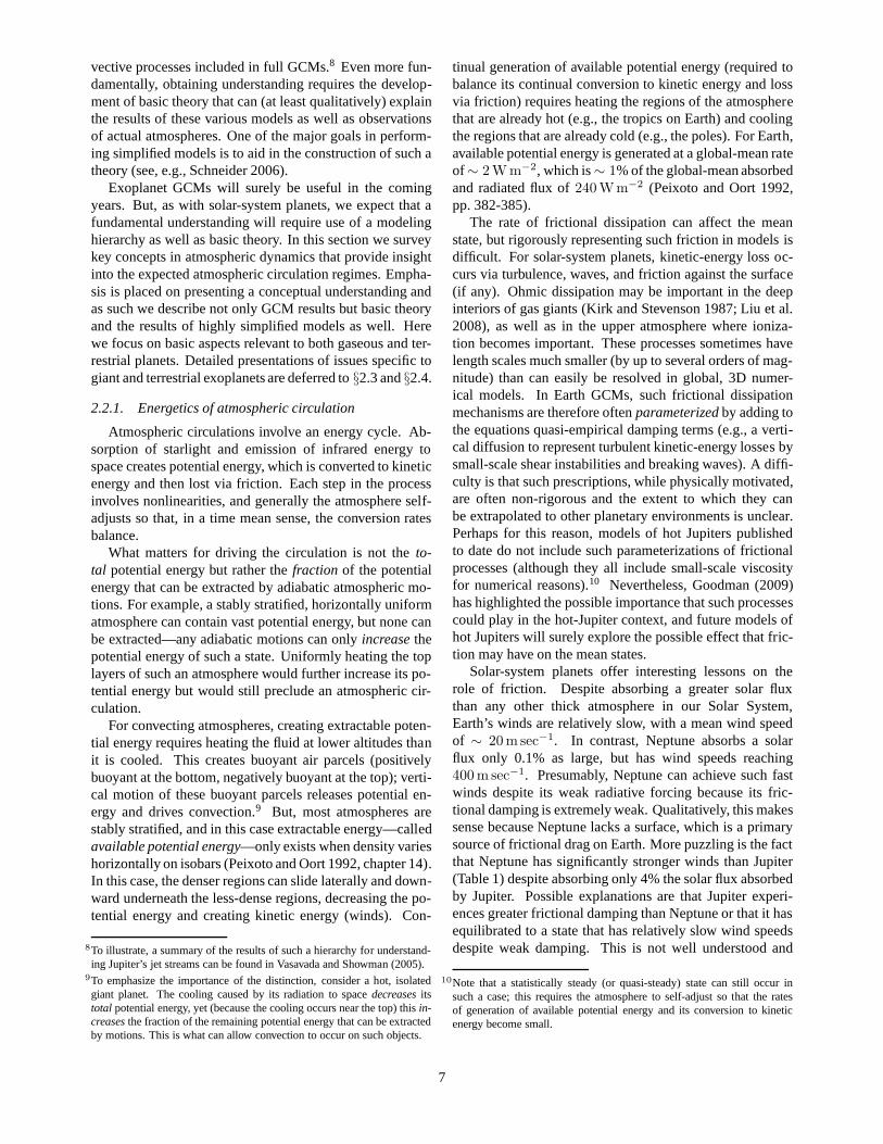
tinual generation of available potential energy (requiredtobalance its continual conversion to kinetic energy and lossvia friction) requires heating the regions of the atmospherethat are already hot (e.g., the tropics on Earth) and coolingthe regions that are already cold (e.g., the poles). For Earth,available potential energy is generated at a global-mean rateof∼ 2 W m−2, which is∼ 1% of the global-mean absorbedand radiated flux of240 Wm−2 (Peixoto and Oort 1992,pp. 382-385).

The rate of frictional dissipation can affect the meanstate, but rigorously representing such friction in modelsisdifficult. For solar-system planets, kinetic-energy loss oc-curs via turbulence, waves, and friction against the surface(if any). Ohmic dissipation may be important in the deepinteriors of gas giants (Kirk and Stevenson 1987; Liu et al.2008), as well as in the upper atmosphere where ioniza-tion becomes important. These processes sometimes havelength scales much smaller (by up to several orders of mag-nitude) than can easily be resolved in global, 3D numer-ical models. In Earth GCMs, such frictional dissipationmechanisms are therefore oftenparameterizedby adding tothe equations quasi-empirical damping terms (e.g., a verti-cal diffusion to represent turbulent kinetic-energy losses bysmall-scale shear instabilities and breaking waves). A diffi-culty is that such prescriptions, while physically motivated,are often non-rigorous and the extent to which they canbe extrapolated to other planetary environments is unclear.Perhaps for this reason, models of hot Jupiters publishedto date do not include such parameterizations of frictionalprocesses (although they all include small-scale viscosityfor numerical reasons).10 Nevertheless, Goodman (2009)has highlighted the possible importance that such processescould play in the hot-Jupiter context, and future models ofhot Jupiters will surely explore the possible effect that fric-tion may have on the mean states.

Solar-system planets offer interesting lessons on therole of friction. Despite absorbing a greater solar fluxthan any other thick atmosphere in our Solar System,Earth’s winds are relatively slow, with a mean wind speedof ∼ 20 m sec−1. In contrast, Neptune absorbs a solarflux only 0.1% as large, but has wind speeds reaching400 m sec−1. Presumably, Neptune can achieve such fastwinds despite its weak radiative forcing because its fric-tional damping is extremely weak. Qualitatively, this makessense because Neptune lacks a surface, which is a primarysource of frictional drag on Earth. More puzzling is the factthat Neptune has significantly stronger winds than Jupiter(Table 1) despite absorbing only 4% the solar flux absorbedby Jupiter. Possible explanations are that Jupiter experi-ences greater frictional damping than Neptune or that it hasequilibrated to a state that has relatively slow wind speedsdespite weak damping. This is not well understood and

10Note that a statistically steady (or quasi-steady) state can still occur insuch a case; this requires the atmosphere to self-adjust so that the ratesof generation of available potential energy and its conversion to kineticenergy become small.

7

argues for humility in efforts to model the circulations ofexoplanets.

2.2.2. Timescale arguments for the coupled radiation-dynamics problem

The atmospheric circulation represents a coupled radiation-hydrodynamics problem. The circulation advects the tem-perature field and thereby influences the radiation field; inturn, the radiation field (along with atmospheric opacitiesand surface conditions) determines the atmospheric heatingand cooling rates that drive the circulation. Rigorously at-tacking this problem requires coupled treatment of both ra-diation and dynamics. However, crude insight into the ther-mal response of an atmosphere can be obtained with sim-ple timescale arguments. Supposeτadvect is an advectiontime (e.g., the characteristic time for air to advect acrossahemisphere) andτrad is the radiative time (i.e., the charac-teristic time for radiation to induce large fractional entropychanges). Whenτrad ≪ τadvect, we expect temperature todeviate only slightly from the (spatially varying) radiativeequilibrium temperature structure. Because the radiative-equilibrium temperature typically varies greatly from day-side to nightside (or from equator to pole), this implies thatsuch a planet would exhibit large fractional temperaturecontrasts. On the other hand, whenτrad ≫ τadvect, dynam-ical transport dominates and air will tend to homogenize itsentropy, implying that lateral temperature contrasts shouldbe modest.

In estimating the advection time, one must distinguishnorth-south from east-west advection; east-west advection(relative to the pattern of stellar insolation) will often bedominated by the planetary rotation. For synchronously ro-tating planets, a characteristic horizontal advection time is

τadvect ∼a

U, (27)

whereU is a characteristic horizontal wind speed. A simi-larly crude estimate of the radiative time can be obtained byconsidering a layer of pressure thickness∆p that is slightlyout of radiative equilibrium and radiates to space as a black-body. If the radiative equilibrium temperature isTrad andthe actual temperature isTrad + ∆T , with ∆T ≪ Trad,then the net flux radiated to space is4σT 3

rad∆T and theradiative timescale is (Showman and Guillot 2002; James1994, pp. 65-66)

τrad ∼ ∆p

g

cp4σT 3

. (28)

In deep, optically thick atmospheres where the radiativetransport is diffusive, a more appropriate estimate might bea diffusion time, crudely given byτrad ∼ H2/D, whereHis the vertical height of a thermal perturbation andD is theradiative diffusivity.

Showman et al. (2008b) estimated advective and radia-tive time constants for solar-system planets and found that,as expected, planets withτrad ≫ τadvect generally havesmall horizontal temperature contrasts and vice versa.

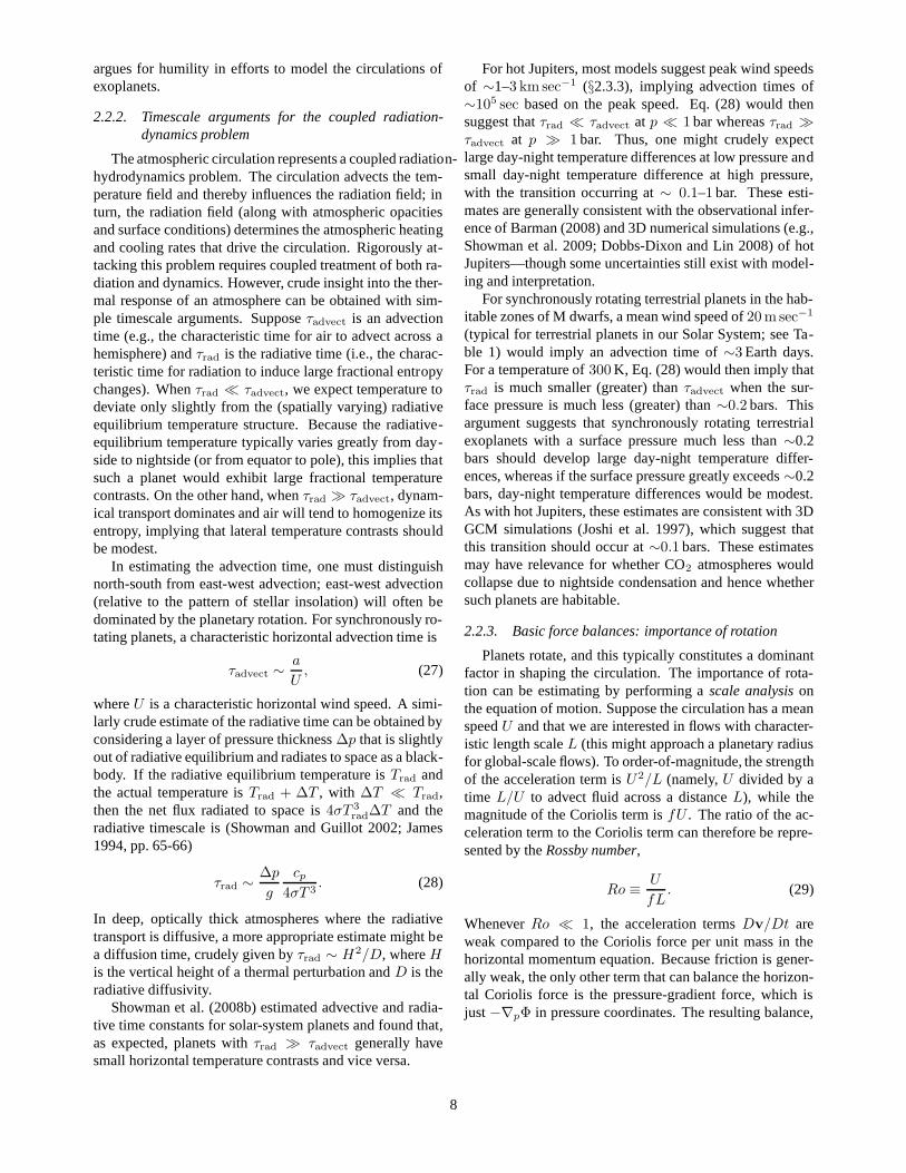
For hot Jupiters, most models suggest peak wind speedsof ∼1–3 km sec−1 (§2.3.3), implying advection times of∼105 sec based on the peak speed. Eq. (28) would thensuggest thatτrad ≪ τadvect at p ≪ 1 bar whereasτrad ≫τadvect at p ≫ 1 bar. Thus, one might crudely expectlarge day-night temperature differences at low pressure andsmall day-night temperature difference at high pressure,with the transition occurring at∼ 0.1–1 bar. These esti-mates are generally consistent with the observational infer-ence of Barman (2008) and 3D numerical simulations (e.g.,Showman et al. 2009; Dobbs-Dixon and Lin 2008) of hotJupiters—though some uncertainties still exist with model-ing and interpretation.

For synchronously rotating terrestrial planets in the hab-itable zones of M dwarfs, a mean wind speed of20 m sec−1

(typical for terrestrial planets in our Solar System; see Ta-ble 1) would imply an advection time of∼3 Earth days.For a temperature of300 K, Eq. (28) would then imply thatτrad is much smaller (greater) thanτadvect when the sur-face pressure is much less (greater) than∼0.2 bars. Thisargument suggests that synchronously rotating terrestrialexoplanets with a surface pressure much less than∼0.2bars should develop large day-night temperature differ-ences, whereas if the surface pressure greatly exceeds∼0.2bars, day-night temperature differences would be modest.As with hot Jupiters, these estimates are consistent with 3DGCM simulations (Joshi et al. 1997), which suggest thatthis transition should occur at∼0.1 bars. These estimatesmay have relevance for whether CO2 atmospheres wouldcollapse due to nightside condensation and hence whethersuch planets are habitable.

2.2.3. Basic force balances: importance of rotation

Planets rotate, and this typically constitutes a dominantfactor in shaping the circulation. The importance of rota-tion can be estimating by performing ascale analysisonthe equation of motion. Suppose the circulation has a meanspeedU and that we are interested in flows with character-istic length scaleL (this might approach a planetary radiusfor global-scale flows). To order-of-magnitude, the strengthof the acceleration term isU2/L (namely,U divided by atime L/U to advect fluid across a distanceL), while themagnitude of the Coriolis term isfU . The ratio of the ac-celeration term to the Coriolis term can therefore be repre-sented by theRossby number,

Ro ≡ U

fL. (29)

WheneverRo ≪ 1, the acceleration termsDv/Dt areweak compared to the Coriolis force per unit mass in thehorizontal momentum equation. Because friction is gener-ally weak, the only other term that can balance the horizon-tal Coriolis force is the pressure-gradient force, which isjust−∇pΦ in pressure coordinates. The resulting balance,

8

calledgeostrophic balance, is given by

fu = −(

∂Φ

∂y

)

p

fv =

(

∂Φ

∂x

)

p

(30)

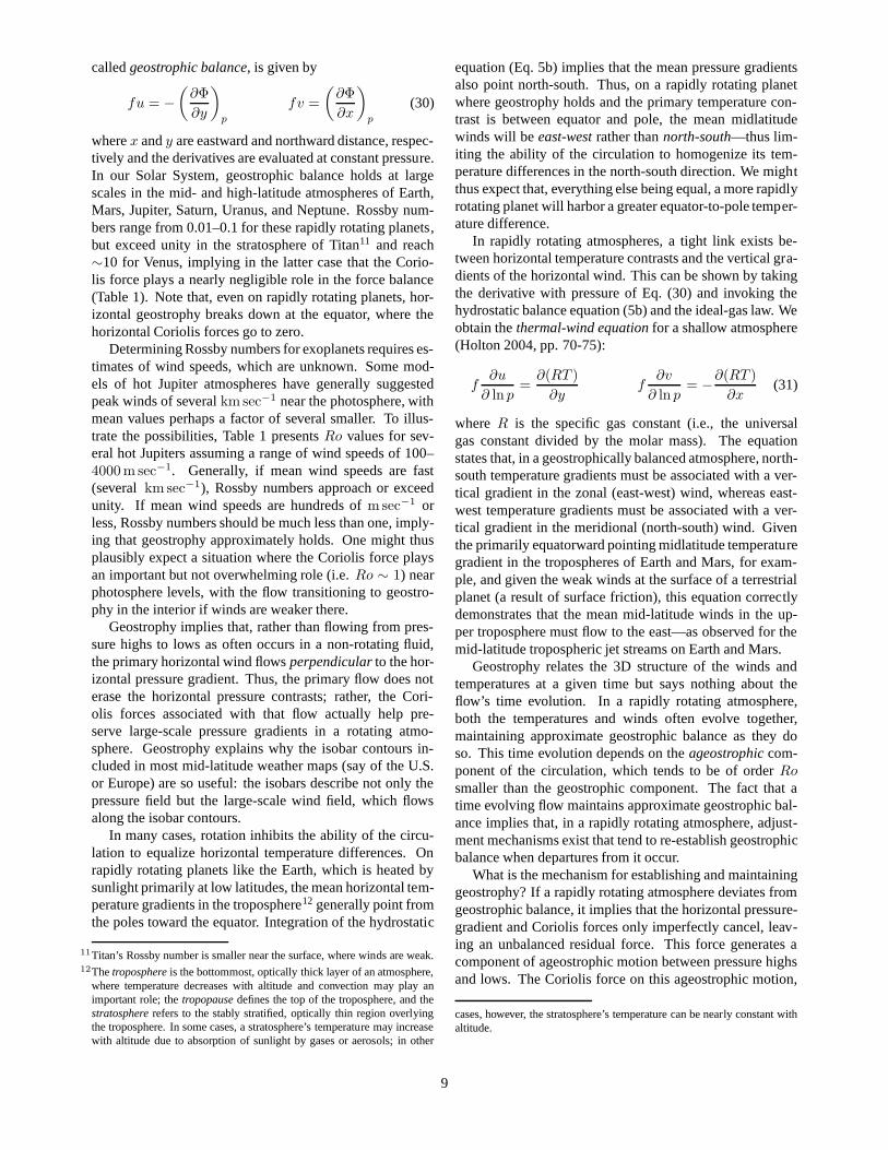
wherex andy are eastward and northward distance, respec-tively and the derivatives are evaluated at constant pressure.In our Solar System, geostrophic balance holds at largescales in the mid- and high-latitude atmospheres of Earth,Mars, Jupiter, Saturn, Uranus, and Neptune. Rossby num-bers range from 0.01–0.1 for these rapidly rotating planets,but exceed unity in the stratosphere of Titan11 and reach∼10 for Venus, implying in the latter case that the Corio-lis force plays a nearly negligible role in the force balance(Table 1). Note that, even on rapidly rotating planets, hor-izontal geostrophy breaks down at the equator, where thehorizontal Coriolis forces go to zero.

Determining Rossby numbers for exoplanets requires es-timates of wind speeds, which are unknown. Some mod-els of hot Jupiter atmospheres have generally suggestedpeak winds of severalkm sec−1 near the photosphere, withmean values perhaps a factor of several smaller. To illus-trate the possibilities, Table 1 presentsRo values for sev-eral hot Jupiters assuming a range of wind speeds of 100–4000 m sec−1. Generally, if mean wind speeds are fast(severalkm sec−1), Rossby numbers approach or exceedunity. If mean wind speeds are hundreds ofmsec−1 orless, Rossby numbers should be much less than one, imply-ing that geostrophy approximately holds. One might thusplausibly expect a situation where the Coriolis force playsan important but not overwhelming role (i.e.Ro ∼ 1) nearphotosphere levels, with the flow transitioning to geostro-phy in the interior if winds are weaker there.

Geostrophy implies that, rather than flowing from pres-sure highs to lows as often occurs in a non-rotating fluid,the primary horizontal wind flowsperpendicularto the hor-izontal pressure gradient. Thus, the primary flow does noterase the horizontal pressure contrasts; rather, the Cori-olis forces associated with that flow actually help pre-serve large-scale pressure gradients in a rotating atmo-sphere. Geostrophy explains why the isobar contours in-cluded in most mid-latitude weather maps (say of the U.S.or Europe) are so useful: the isobars describe not only thepressure field but the large-scale wind field, which flowsalong the isobar contours.

In many cases, rotation inhibits the ability of the circu-lation to equalize horizontal temperature differences. Onrapidly rotating planets like the Earth, which is heated bysunlight primarily at low latitudes, the mean horizontal tem-perature gradients in the troposphere12 generally point fromthe poles toward the equator. Integration of the hydrostatic

11Titan’s Rossby number is smaller near the surface, where winds are weak.12Thetroposphereis the bottommost, optically thick layer of an atmosphere,

where temperature decreases with altitude and convection may play animportant role; thetropopausedefines the top of the troposphere, and thestratosphererefers to the stably stratified, optically thin region overlyingthe troposphere. In some cases, a stratosphere’s temperature may increasewith altitude due to absorption of sunlight by gases or aerosols; in other

equation (Eq. 5b) implies that the mean pressure gradientsalso point north-south. Thus, on a rapidly rotating planetwhere geostrophy holds and the primary temperature con-trast is between equator and pole, the mean midlatitudewinds will beeast-westrather thannorth-south—thus lim-iting the ability of the circulation to homogenize its tem-perature differences in the north-south direction. We mightthus expect that, everything else being equal, a more rapidlyrotating planet will harbor a greater equator-to-pole temper-ature difference.

In rapidly rotating atmospheres, a tight link exists be-tween horizontal temperature contrasts and the vertical gra-dients of the horizontal wind. This can be shown by takingthe derivative with pressure of Eq. (30) and invoking thehydrostatic balance equation (5b) and the ideal-gas law. Weobtain thethermal-wind equationfor a shallow atmosphere(Holton 2004, pp. 70-75):

f∂u

∂ ln p=∂(RT )

∂yf∂v

∂ ln p= −∂(RT )

∂x(31)

whereR is the specific gas constant (i.e., the universalgas constant divided by the molar mass). The equationstates that, in a geostrophically balanced atmosphere, north-south temperature gradients must be associated with a ver-tical gradient in the zonal (east-west) wind, whereas east-west temperature gradients must be associated with a ver-tical gradient in the meridional (north-south) wind. Giventhe primarily equatorward pointing midlatitude temperaturegradient in the tropospheres of Earth and Mars, for exam-ple, and given the weak winds at the surface of a terrestrialplanet (a result of surface friction), this equation correctlydemonstrates that the mean mid-latitude winds in the up-per troposphere must flow to the east—as observed for themid-latitude tropospheric jet streams on Earth and Mars.

Geostrophy relates the 3D structure of the winds andtemperatures at a given time but says nothing about theflow’s time evolution. In a rapidly rotating atmosphere,both the temperatures and winds often evolve together,maintaining approximate geostrophic balance as they doso. This time evolution depends on theageostrophiccom-ponent of the circulation, which tends to be of orderRosmaller than the geostrophic component. The fact that atime evolving flow maintains approximate geostrophic bal-ance implies that, in a rapidly rotating atmosphere, adjust-ment mechanisms exist that tend to re-establish geostrophicbalance when departures from it occur.

What is the mechanism for establishing and maintaininggeostrophy? If a rapidly rotating atmosphere deviates fromgeostrophic balance, it implies that the horizontal pressure-gradient and Coriolis forces only imperfectly cancel, leav-ing an unbalanced residual force. This force generates acomponent of ageostrophic motion between pressure highsand lows. The Coriolis force on this ageostrophic motion,

cases, however, the stratosphere’s temperature can be nearly constant withaltitude.

9

TABLE 1

PLANETARY PARAMETERS

Planet a∗ Rotation period♯ Ω gravityℵ F2⋆ T♠

e H†p U‡ Ro¶ LD/a

♣ Lβ/a3

(103 km) (Earth days) (rad sec−1) (msec−2) (W m−2) (K) (km) (msec−1)

Venus 6.05 243 3 × 10−7 8.9 2610 232 5 ∼ 20 10 70 7Earth 6.37 1 7.27 × 10−5 9.82 1370 255 7 ∼ 20 0.1 0.3 0.5Mars 3.396 1.025 7.1 × 10−5 3.7 590 210 11 ∼ 20 0.1 0.6 0.6Titan 2.575 16 4.5 × 10−6 1.4 15 85 18 ∼ 20 2 10 3Jupiter 71.4 0.4 1.7 × 10−4 23.1 50 124 20 ∼ 40 0.02 0.03 0.1Saturn 60.27 0.44 1.65 × 10−4 8.96 15 95 39 ∼ 150 0.06 0.03 0.3Uranus 25.56 0.72 9.7 × 10−5 8.7 3.7 59 25 ∼ 100 0.1 0.1 0.4Neptune 24.76 0.67 1.09 × 10−4 11.1 1.5 59 20 ∼ 200 0.1 0.1 0.6

WASP-12b 128 1.09 6.7 × 10−5 11.5 8.8 × 106 2500 800 - 0.01–0.3 0.1 0.2–1.5HD 189733b 81 2.2 3.3 × 10−5 22.7 4.7 × 105 1200 200 - 0.03–1 0.3 0.4–3HD 149026b 47 2.9 2.5 × 10−5 21.9 1.8 × 106 1680 280 - 0.06–2 0.8 0.6–4HD 209458b 94 3.5 2.1 × 10−5 10.2 1.0 × 106 1450 520 - 0.04–1 0.4 0.5–3TrES-2 87 2.4 2.9 × 10−5 21 1.1 × 106 1475 260 - 0.03–1 0.3 0.4–3TrES-4 120 3.5 2.0 × 10−5 7.8 2.5 × 106 1825 870 - 0.03–1 0.4 0.4–3HAT-P-7b 97 2.2 3.3 × 10−5 25 4.7 × 106 2130 320 - 0.02–1 0.3 0.4–3GJ 436b 31 2.6 2.8 × 10−5 9.8 4.3 × 104 660 250 - 0.1–3 0.7 0.8–5HAT-P-2b 68 5.6 1.3 × 10−5 248 9.5 × 105 1400 21 - 0.1–3 1 0.8–5Corot-Exo-4b 85 9.2 7.9 × 10−6 13.2 3.0 × 105 1080 300 - 0.1–4 1 0.9–5

NOTE.—∗Equatorial planetary radius.♯Assumes synchronous rotation for exoplanets.ℵ Equatorial gravity at the surface.2Mean incident stellar flux.♠Global-average blackbody emission temperature, which for exoplanets is calculated from Eq. (60) assuming zero albedo.†Pressure scale height, evaluated at temperatureTe. ‡Rough estimates of mean horizontal wind speed. Estimates for Venus and Titan are in the high-altitude superrotating jet; both planets have weaker winds (fewm sec−1) in the bottom scale height. In all cases, peak winds exceed the listed values by factors of two or more.¶Rossby number, evaluated in mid-latitudes usingwind values listed in Table andL ∼ 2000 km for Earth, Mars, and Titan,6000 km for Venus, and104 km for Jupiter, Saturn, Uranus, and Neptune. For exoplanets, wepresent a range of possible values evaluated withL = a and winds from 100 to4000 m sec−1. ♣Ratio of Rossby deformation radius to planetary radius, evaluted inmid-latitudes withH equal to the pressure scale height andN appropriate for a vertically isothermal temperature profile. 3Ratio of Rhines length (Eq. 44) to planetaryradius, calculated using the equatorial value ofβ and the wind speeds listed in the Table.

10

and the alteration of the pressure contrasts caused by theageostrophic wind, act to re-establish geostrophy.

To give a concrete example, imagine an atmosphere withzero winds and a localized circular region of high surfacepressure surrounded on all sides by lower surface pres-sure. This state has an unbalanced pressure-gradient force,which would induce a horizontal acceleration of fluid ra-dially away from the high-pressure region. The horizontalCoriolis force on this outward motion causes a lateral de-flection (to the right in the northern hemisphere and left inthe southern hemisphere13), leading to a vortex surroundingthe high-pressure region. The Coriolis force on this vor-tical motion points radially toward the high-pressure cen-ter, resisting its lateral expansion. This process continuesuntil the inward-pointing Coriolis force balances the out-ward pressure-gradient force—hence establishing geostro-phy and inhibiting further expansion. Although this is anextreme example, radiative heating/cooling, friction, andother forcings gradually push the atmosphere away fromgeostrophy, and the process described above re-establishesit.

This process, calledgeostrophic adjustment, tends to oc-cur with a natural length scale comparable to the Rossbyradius of deformation, given in a 3D system by

LD =NH

f(32)

whereN is Brunt-Vaisala frequency (Eq. 6),H is the verti-cal scale of the flow, andf is the Coriolis parameter. Thus,geostrophic adjustment naturally generates large-scale at-mospheric flow structures with horizontal sizes compara-ble to the deformation radius (see Holton (2004) or Vallis(2006) for a detailed treatment).

Equation (31), as written, applies to atmospheres thatare vertically thin compared to their horizontal dimensions(i.e., shallow atmospheres). However, a non-shallow analogof Eq. (31) can be obtained by considering the 3D vortic-ity equation. In a geostrophically balanced fluid where thefriction force is weak, the vorticity balance is given by (seePedlosky 1987, p. 43)

2(Ω · ∇)u − 2Ω(∇ · u) = −∇ρ×∇pρ2

, (33)

whereΩ is the planetary rotation vector andu is the 3Dwind velocity. The term on the right, called the baroclinicterm, is nonzero when density varies on constant-pressuresurfaces. In the interior of a giant planet, however, convec-tion tends to homogenize the entropy, in which case frac-tional density variations on isobars are extremely small.Such a fluid, where surfaces of constantp and ρ align,is called a barotropic fluid. In this case the right side ofEq. (33) can be neglected, leading to the compressible-fluid

13Northern and southern hemispheres are here defined as those whereΩ ·

k > 0 and< 0, respectively, whereΩ andk are the planetary rotationvector and local vertical (upward) unit vector.

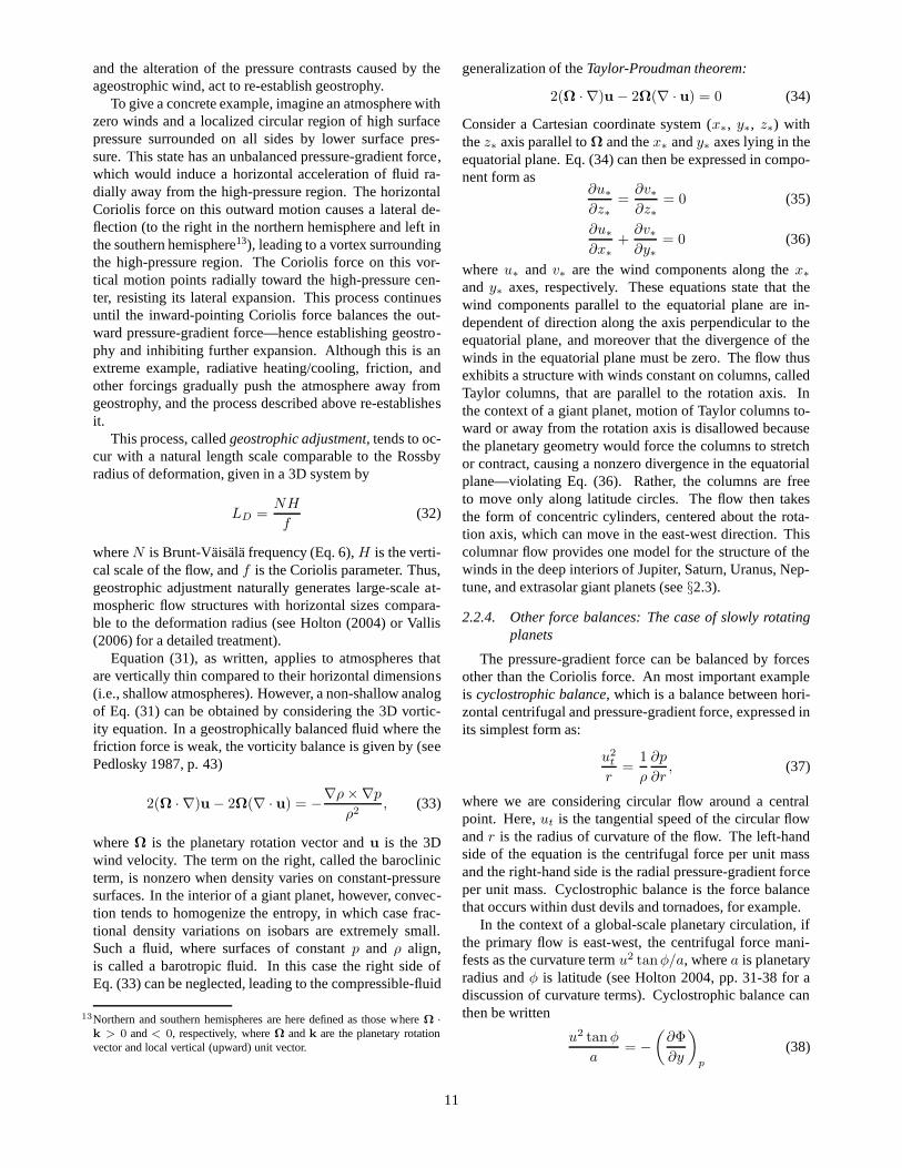
generalization of theTaylor-Proudman theorem:

2(Ω · ∇)u − 2Ω(∇ · u) = 0 (34)

Consider a Cartesian coordinate system (x∗, y∗, z∗) withthez∗ axis parallel toΩ and thex∗ andy∗ axes lying in theequatorial plane. Eq. (34) can then be expressed in compo-nent form as

∂u∗∂z∗

=∂v∗∂z∗

= 0 (35)

∂u∗∂x∗

+∂v∗∂y∗

= 0 (36)

whereu∗ and v∗ are the wind components along thex∗and y∗ axes, respectively. These equations state that thewind components parallel to the equatorial plane are in-dependent of direction along the axis perpendicular to theequatorial plane, and moreover that the divergence of thewinds in the equatorial plane must be zero. The flow thusexhibits a structure with winds constant on columns, calledTaylor columns, that are parallel to the rotation axis. Inthe context of a giant planet, motion of Taylor columns to-ward or away from the rotation axis is disallowed becausethe planetary geometry would force the columns to stretchor contract, causing a nonzero divergence in the equatorialplane—violating Eq. (36). Rather, the columns are freeto move only along latitude circles. The flow then takesthe form of concentric cylinders, centered about the rota-tion axis, which can move in the east-west direction. Thiscolumnar flow provides one model for the structure of thewinds in the deep interiors of Jupiter, Saturn, Uranus, Nep-tune, and extrasolar giant planets (see§2.3).

2.2.4. Other force balances: The case of slowly rotatingplanets

The pressure-gradient force can be balanced by forcesother than the Coriolis force. An most important exampleis cyclostrophic balance, which is a balance between hori-zontal centrifugal and pressure-gradient force, expressed inits simplest form as:

u2t

r=

1

ρ

∂p

∂r, (37)

where we are considering circular flow around a centralpoint. Here,ut is the tangential speed of the circular flowandr is the radius of curvature of the flow. The left-handside of the equation is the centrifugal force per unit massand the right-hand side is the radial pressure-gradient forceper unit mass. Cyclostrophic balance is the force balancethat occurs within dust devils and tornadoes, for example.

In the context of a global-scale planetary circulation, ifthe primary flow is east-west, the centrifugal force mani-fests as the curvature termu2 tanφ/a, wherea is planetaryradius andφ is latitude (see Holton 2004, pp. 31-38 for adiscussion of curvature terms). Cyclostrophic balance canthen be written

u2 tanφ

a= −

(

∂Φ

∂y

)

p

(38)

11

This is the force balance relevant on Venus, for exam-ple, where a strong zonal jet with peak speeds reach-ing ∼100 m sec−1 dominates the stratospheric circulation(Gierasch et al. 1997). Eq. (38) can be differentiated withrespect to pressure to yield a cyclostrophic version of thethermal-wind equation:

∂(u2)

∂ ln p= − a

tanφ

∂(RT )

∂y, (39)

where hydrostatic balance and the ideal-gas law have beeninvoked.

Thus, on a slowly rotating, cyclostrophically balancedplanet like Venus, Eq. (39) would indicate that varia-tion of the zonal winds with height requires latitudinaltemperature gradients as occur with geostrophic balance.Note, however, that for zonal winds whose strength in-creases with height, the latitudinal temperature gradientsfor cyclostrophic balance point equatorwardregardlessofwhether the zonal winds are east or west. This differs fromgeostrophy, where latitudinal temperature gradients wouldpoint equatorward for a zonal wind that becomes moreeastward with height but poleward for a zonal wind thatbecomes more westward with height.

2.2.5. What controls vertical velocities?

In atmospheres, mean vertical velocities associated withthe large-scale circulation tend to be much smaller than hor-izontal velocities. This results from several factors:

Large aspect ratio:Atmospheres generally have horizon-tal dimensions greatly exceeding their vertical dimensions,which leads to a strong geometric constraint on vertical mo-tions. To illustrate, supposeU/c ≪ 1, where c is thesound speed, and the continuity equation can be approxi-mated in 3D by the incompressibility condition∇ · u =∂u/∂x+ ∂v/∂y+ ∂w/∂z = 0. To order of magnitude, thehorizontal terms can be approximated asU/L and the verti-cal term can be approximated asW/H , whereL andH arethe horizontal and vertical scales andU andW are the char-acteristic magnitudes of the horizontal and vertical wind.This then suggests a vertical velocity of approximately

W ∼ H

LU (40)

On a typical terrestrial planet,U ∼ 10 m sec−1, L ∼1000 km, andH ∼ 10 km, which would suggestW ∼0.1 m sec−1, two orders of magnitude smaller than hori-zontal velocities. However, this estimate ofW is an upperlimit, since partial cancellation can occur between∂u/∂xand ∂v/∂y, and indeed for most atmospheres Eq. (40)greatly overestimates their mean vertical velocities. OnEarth, for example, mean midlatitude vertical velocities onlarge scales (∼103 km) are actually∼10−2 msec−1 in thetroposphere and∼10−3 msec−1 in the stratosphere, muchsmaller than suggested by Eq. (40).

Suppression of vertical motion by rotation:The geostrophicvelocity flows perpendicular to the horizontal pressure gra-

dient, which implies that a large fraction of this flow can-not cause horizontal divergence or convergence (as neces-sary to allow vertical motions). However, theageostrophiccomponent of the flow, which isO(Ro) smaller thanthe geostrophic component, can cause horizontal conver-gence/divergence. Thus, to order-of-magnitude one mightexpectW ∼ RoU/L. Considering the geostrophic flowand taking the curl of Eq. (30), we can show that the hori-zontal divergence of the horizontal geostrophic wind is

∇p · vG =β

fv =

v

a tanφ(41)

where in the rightmost expressionβ/f has been evalu-ated assuming spherical geometry. To order of magnitude,v ∼ U . Eq. (41) then implies that to order-of-magnitudethe horizontal flow divergence is notU/L but ratherU/a.On many planets, the dominant flow structures are smallerthan the planetary radius (e.g.,L/a ∼ 0.1–0.2 for Earth,Jupiter, and Saturn). This implies that the horizontal di-vergence of the geostrophic flow is∼L/a smaller than theestimate in Eq. (40). Taken together, these constraints sug-gest that rapid rotation can suppress vertical velocities byclose to an order of magnitude. For Earth parameters, theestimates implyW ∼ 0.01 m sec−1, similar to the meanvertical velocities in Earth’s troposphere.

Suppression of vertical motion by stable stratification:Most atmospheres are stably stratified, implying that en-tropy (potential temperature) increases with height. Adia-batic expansion/contraction in ascending (descending) airwould cause temperature at a given height to decrease (in-crease) over time. In the absence of radiation, such steadyflow patterns are unsustainable because they induce densityvariations that resist the motion—ascending air becomesdenser and descending air becomes less dense than thesurroundings. Thus, in stably stratified atmospheres, theradiative heating/cooling rate exerts major control over therate of vertical ascent/decent. Steady vertical motion canonly occur as fast as radiation can remove the temperaturevariations caused by the adiabatic ascent/descent (Show-man et al. 2008a), when conduction is negligible. The ideacan be quantified by rewriting the thermodynamic energyequation (Eq. 5d) in terms of the Brunt-Vaisala frequency:

∂T

∂t+ v · ∇pT − ω

H2pN

2

Rp=qnet

cp(42)

whereHp is the pressure scale height. An upper limit on themagnitude of the vertical velocity is obtained by equatingthe right side to the last term on the left side. Convertingto velocity expressed in height units, we obtain (Showmanet al. 2008a; Showman and Guillot 2002)

W ∼ qnet

cp

R

HpN2. (43)

For Earth’s midlatitude troposphere,Hp ∼ 10 km, N ∼0.01 sec−1, and qnet/cp ∼ 3 × 10−5 K sec−1, implying

12

W ∼ 10−2 msec−1. In the stratosphere, however, the heat-ing rate is lower, and the stable stratification is greater, lead-ing to values ofW ∼ 10−3 msec−1.

For a canonical hot Jupiter with a 3-day rotation pe-riod, horizontal wind speeds ofkm sec−1 imply Rossbynumbers of∼1, and for scale heights of∼300 km (Ta-ble 1) and horizontal length scales of a planetary ra-dius, one thus estimatesRoUH/L ∼ 10 m sec−1. Like-wise, forR = 3700 J kg−1 K−1, Hp ∼ 300 km, N ≈0.005 sec−1 (appropriate for an isothermal layer on a hotJupiter with surface gravity of20 m sec−1), andqnet/cp ∼10−2K sec−1 (perhaps appropriate for photospheres of atypical hot Jupiter), Eq. (43) suggests mean vertical speedsof W ∼ 10 m sec−1 (Showman and Guillot 2002; Show-man et al. 2008a). Thus, despite the fact that the circula-tion on hot Jupiters occurs in a radiative zone expected tobe stably stratified over most of the planet, vertical over-turning can occur near the photosphere over timescales ofHp/W ∼ 105 sec. Because the interior of a multi-Gyr-old hot Jupiter transports an intrinsic flux of only∼ 10–100 Wm−2 (as compared with typically∼ 105 W m−2 inthe layer where starlight is absorbed and infrared radia-tion escapes to space), the net heatingqnet should decreaserapidly with depth. The mean vertical velocities should thusplummet with depth, leading to very long overturning timesin the bottom part of the radiative zone.

2.2.6. Effect of eddies: jet streams and banding

Although turbulence is a challenging problem, severaldecades of work in the fields of fluid mechanics and at-mosphere/ocean dynamics have led to a basic understand-ing of turbulent flows and how they interact with planetaryrotation. In a 3D turbulent flow, vortex stretching and fil-amentation drives a fluid’s kinetic energy to smaller andsmaller length scales, where it can finally be removed byviscous dissipation. This process, the so-calledforwarden-ergy cascade, occurs when turbulence has scales smallerthan a fraction of a pressure scale height (∼10 km for Earth,∼200 km for hot Jupiters). On global scales, however, at-mospheres are quasi-two-dimensional, with horizontal flowdimensions exceeding vertical flow dimensions by typicallyfactors of∼100. In this quasi-2D regime, vortex stretch-ing is inhibited, and other nonlinear processes, such as vor-tex merging, assume a more prominent role, forcing energyto undergo aninversecascade from small to large scales(Vallis 2006, pp. 349-361). This process has been well-documented in idealized laboratory and numerical exper-iments (e.g., Tabeling 2002) and helps explain the emer-gence of large-scale jets and vortices from small-scale tur-bulent forcing in planetary atmospheres.

Where the Coriolis parameterf is approximately con-stant, this process generally produces turbulence that is hor-izontally isotropic, that is, turbulence without any preferreddirectionality (north-south versus east-west). This couldexplain the existence of some quasi-circular vortices onJupiter and Saturn, for example; however, it fails to explain

the existence of numerous jet streams on Jupiter, Saturn,Uranus, Neptune, and the terrestrial planets. On the otherhand, Rhines (1975) realized that the variation off with lat-itude leads to anisotropy, causing elongation of structuresin the east-west direction relative to the north-south direc-tion. This anisotropy can cause the energy to reorganizeinto east-west oriented jet streams with a characteristic lat-itudinal length scale

Lβ = π

(

U

β

)1/2

(44)

whereU is a mean wind speed andβ ≡ df/dy is the gra-dient of the Coriolis parameter with northward distancey.This length is called the Rhines scale.

Numerous idealized studies of 2D turbulent flow forcedby injection of small-scale turbulence have demonstratedjet formation by this mechanism (Williams 1978; Cho andPolvani 1996a; Huang and Robinson 1998; Marcus et al.2000; Vasavada and Showman 2005). Figure 1 illustratesan example. In 2D non-divergent numerical simulations offlow energized by small-scale turbulence, the flow remainsisotropic at low rotation rates (Fig. 1, left) but developsbanded structure at high rotation rates (Fig. 1, right). Asshown in Fig. 2, the number of jets in such simulations in-creases as the wind speed decreases, qualitatively consistentwith Eq. (44).

The Rhines scale can be interpreted as a transition scalebetween the regimes of turbulence and Rossby waves,which are a large-scale wave solution to the dynamicalequations in the presence of non-zeroβ. Considering thesimplest possible case of an unforced 2D non-divergentfluid (§2.1.3), the vorticity equation reads

∂ζ

∂t+ v · ∇ζ + vβ = 0, (45)

whereζ is the relative vorticity,v is the horizontal veloc-ity vector, andv is the northward velocity component. Therelative vorticity has characteristic scaleU/L, and so thenonlinear term has characteristic scaleU2/L2. Theβ termhas characteristic scaleβU . Comparison between these twoterms shows that, for length scales smaller than the Rhinesscale, the nonlinear term dominates, implying the domi-nance of nonlinear vorticity advection. For scales exceed-ing the Rhines scale, the linearvβ term dominates over thenonlinear term, and Rossby waves are the primary solutionsto the equations.14

How does jet formation occur at the Rhines scale? In

14Adopting a streamfunctionψ defined byu = −∂ψ/∂y andv = ∂ψ/∂x,the 2D non-divergent vorticity equation can be written∂∇2ψ/∂t +β∂ψ/∂x = 0 when the nonlinear term is neglected. In Cartesian ge-ometry with constantβ, this equation has wave solutions with a dispersionrelationshipω = −βk2/(k2 + l2) whereω is the oscillation frequencyandk andl are the wavenumbers (2π over the wavelength) in the eastwardand northward directions, respectively. These are Rossby waves, whichhave a westward phase speed and a frequency that depends on the waveorientation.

13

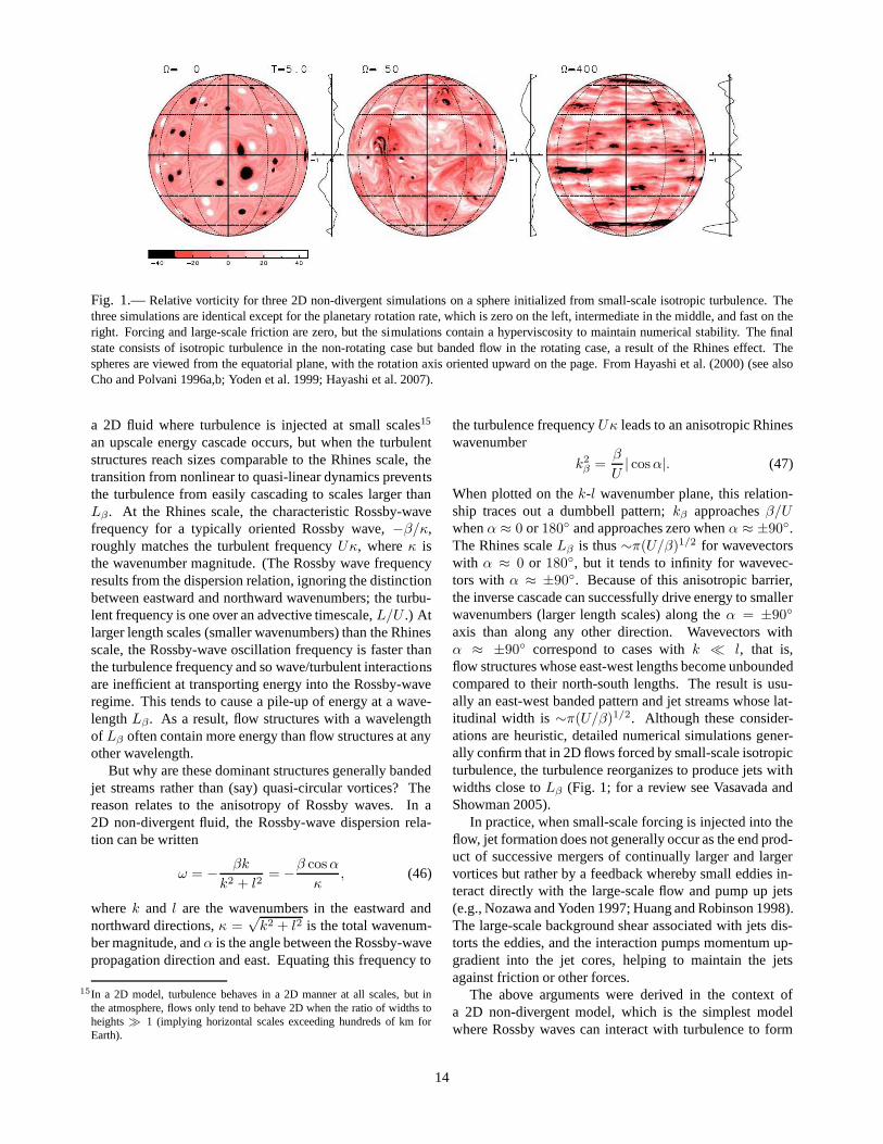
Fig. 1.—Relative vorticity for three 2D non-divergent simulationson a sphere initialized from small-scale isotropic turbulence. Thethree simulations are identical except for the planetary rotation rate, which is zero on the left, intermediate in the middle, and fast on theright. Forcing and large-scale friction are zero, but the simulations contain a hyperviscosity to maintain numerical stability. The finalstate consists of isotropic turbulence in the non-rotatingcase but banded flow in the rotating case, a result of the Rhines effect. Thespheres are viewed from the equatorial plane, with the rotation axis oriented upward on the page. From Hayashi et al. (2000) (see alsoCho and Polvani 1996a,b; Yoden et al. 1999; Hayashi et al. 2007).

a 2D fluid where turbulence is injected at small scales15

an upscale energy cascade occurs, but when the turbulentstructures reach sizes comparable to the Rhines scale, thetransition from nonlinear to quasi-linear dynamics preventsthe turbulence from easily cascading to scales larger thanLβ. At the Rhines scale, the characteristic Rossby-wavefrequency for a typically oriented Rossby wave,−β/κ,roughly matches the turbulent frequencyUκ, whereκ isthe wavenumber magnitude. (The Rossby wave frequencyresults from the dispersion relation, ignoring the distinctionbetween eastward and northward wavenumbers; the turbu-lent frequency is one over an advective timescale,L/U .) Atlarger length scales (smaller wavenumbers) than the Rhinesscale, the Rossby-wave oscillation frequency is faster thanthe turbulence frequency and so wave/turbulent interactionsare inefficient at transporting energy into the Rossby-waveregime. This tends to cause a pile-up of energy at a wave-lengthLβ. As a result, flow structures with a wavelengthof Lβ often contain more energy than flow structures at anyother wavelength.

But why are these dominant structures generally bandedjet streams rather than (say) quasi-circular vortices? Thereason relates to the anisotropy of Rossby waves. In a2D non-divergent fluid, the Rossby-wave dispersion rela-tion can be written

ω = − βk

k2 + l2= −β cosα

κ, (46)

wherek and l are the wavenumbers in the eastward andnorthward directions,κ =

√k2 + l2 is the total wavenum-

ber magnitude, andα is the angle between the Rossby-wavepropagation direction and east. Equating this frequency to

15In a 2D model, turbulence behaves in a 2D manner at all scales,but inthe atmosphere, flows only tend to behave 2D when the ratio of widths toheights≫ 1 (implying horizontal scales exceeding hundreds of km forEarth).

the turbulence frequencyUκ leads to an anisotropic Rhineswavenumber

k2β =

β

U| cosα|. (47)

When plotted on thek-l wavenumber plane, this relation-ship traces out a dumbbell pattern;kβ approachesβ/Uwhenα ≈ 0 or 180 and approaches zero whenα ≈ ±90.The Rhines scaleLβ is thus∼π(U/β)1/2 for wavevectorswith α ≈ 0 or 180, but it tends to infinity for wavevec-tors withα ≈ ±90. Because of this anisotropic barrier,the inverse cascade can successfully drive energy to smallerwavenumbers (larger length scales) along theα = ±90

axis than along any other direction. Wavevectors withα ≈ ±90 correspond to cases withk ≪ l, that is,flow structures whose east-west lengths become unboundedcompared to their north-south lengths. The result is usu-ally an east-west banded pattern and jet streams whose lat-itudinal width is∼π(U/β)1/2. Although these consider-ations are heuristic, detailed numerical simulations gener-ally confirm that in 2D flows forced by small-scale isotropicturbulence, the turbulence reorganizes to produce jets withwidths close toLβ (Fig. 1; for a review see Vasavada andShowman 2005).

In practice, when small-scale forcing is injected into theflow, jet formation does not generally occur as the end prod-uct of successive mergers of continually larger and largervortices but rather by a feedback whereby small eddies in-teract directly with the large-scale flow and pump up jets(e.g., Nozawa and Yoden 1997; Huang and Robinson 1998).The large-scale background shear associated with jets dis-torts the eddies, and the interaction pumps momentum up-gradient into the jet cores, helping to maintain the jetsagainst friction or other forces.

The above arguments were derived in the context ofa 2D non-divergent model, which is the simplest modelwhere Rossby waves can interact with turbulence to form

14

Fig. 2.—Zonal-mean zonal winds versus latitude for a series of global, 2D non-divergent simulations performed on a sphere showingthe correlation between jet speed and jet width. The simulations are forced by small-scale turbulence and damped by a linear drag. Eachsimulation uses different forcing and friction parametersand equilibrates to a different mean wind speed, ranging from fast on the left toslow on the right. Simulations with faster jets have fewer jets and vice versa; the jet widths approximately scale with the Rhines length.From Huang and Robinson (1998).

jets. Such a model lacks gravity waves and has an infi-nite deformation radiusLD (Eqs. 16 and 32). It is possi-ble to extend the above ideas to one-layer models exhibit-ing gravity waves and a finite deformation radius, such asthe shallow-water model. Doing so shows that, as long asβ is strong, jets dominate when the deformation radius islarge (as in the 2D non-divergent model); however, the flowbecomes more isotropic (dominated by vortices rather thanjets) when the deformation radius is sufficiently smallerthan(U/β)1/2 (e.g., Okuno and Masuda 2003; Smith 2004;Showman 2007).

On a spherical planet,β = 2Ωa−1 cosφ, which impliesthat a planet should have a number of jet streams roughlygiven by

Njet ∼(

2Ωa

U

)1/2

. (48)

These considerations do a reasonable job of predictingthe latitudinal separations and total number of jets that ex-ist on planets in our Solar System. Given the known windspeeds (Table 1) and values ofβ, the Rhines scale predicts∼ 20 jet streams on Jupiter/Saturn, 4 jet streams on Uranusand Neptune, and 7 jet streams on Earth. This is similarto the observed numbers (∼ 20 on Jupiter and Saturn, 3on Uranus and Neptune, and 3 to 7 on Earth dependingon how they are defined16) Moreover, the scale-dependentanisotropy—with quasi-isotropic turbulence at small scalesand banded flow at large scales—is readily apparent onsolar-system planets. Fig. 3 illustrates an example for Sat-urn: small-scale structures (e.g., the cloud-covered vorticesthat manifest as small dark spots in the figure) are relativelycircular, whereas the large-scale structures are banded.

16In Earth’s troposphere, an instantaneous snapshot typically shows distinctsubtropical and high-latitude jets in each hemisphere, with weaker flow be-tween these jets and westward flow at the equator. The jet latitudes exhibitlarge excursions in longitude and time, however, and when a time- andlongitude average is performed, only a single local maximumin eastwardflow exists in each hemisphere, with westward flow at the equator.

These considerations yield insight into the degree ofbanding and size of dominant flow structures to be ex-pected on exoplanets. Equation (48) suggests that the num-ber of bands scales asΩ1/2, so rapidly rotating exoplan-ets will tend to exhibit numerous strongly banded jets,whereas slowly rotating planets will exhibit fewer jets withweaker banding. Moreover, for a given rotation rate, planetswith slower winds should exhibit more bands than planetswith faster winds. Hot Jupiters are expected to be tidallylocked, implying rotation rates of typically a few days.Although wind speeds on hot Jupiters are unknown, vari-ous numerical models have obtained (or assumed) speedsof ∼0.5–3km sec−1 (Showman and Guillot 2002; Cooperand Showman 2005; Langton and Laughlin 2007; Dobbs-Dixon and Lin 2008; Menou and Rauscher 2009; Cho et al.2003, 2008). Inserting these values into Eq. (48) impliesNjet ∼ 1–2. Consistent with these arguments, numeri-cal models have obtained typically∼1–3 broad jets. Thus,due to a combination of their slower rotation and presumedfaster wind speeds, hot Jupiters should have only a smallnumber of broad jets—unlike Jupiter and Saturn. If thewind speeds are much slower, and/or rotation rates muchgreater than assumed here, the number of bands would belarger.

2.2.7. Role of eddies in 3D atmospheres

Although atmospheres behave in a quasi-2D manner onlarge scales due to large horizontal:vertical aspect ratios,small Rossby numbers, and stable stratification, they are ofcourse three dimensional, and as a result they can experi-ence both upscale and downscale energy cascades depend-ing on the length scales of the turbulence and other factors.Nevertheless, the basic mechanism discussed above for theinteraction of turbulence and theβ effect still applies andsuggests that even 3D atmospheres can generally exhibit abanded structure with a characteristic length scale close toLβ. Consistent with this idea, numerical simulations showthat banding can indeed occur in 3D even whenβ is the only

15

Fig. 3.—Saturn’s north polar region as imaged by the Cassini Visibleand Infrared Mapping Spectrometer at 5µm wavelengths. Atthis wavelength, scattered sunlight is negligible; brightregions are cloud-free regions where thermal emission escapes from the deep(∼ 3 − 5 bar) atmosphere, whereas dark region are covered by thick clouds that block this thermal radiation. Note the scale-dependentanisotropy: small-scale features tend to be circular, whereas the large-scale features are banded. This phenomenon results directly fromthe Rhines effect (see text). [Photo credit: NASA/VIMS/BobBrown/Kevin Baines.]

source of anisotropy (e.g., Sayanagi et al. 2008; Lian andShowman 2009). Nevertheless, on real planets, banding canalso result from anisotropic forcing—such as the fact thatsolar heating is primarily a function of latitude rather thanlongitude on rapidly rotating planets like Earth and Mars.

A variety of studies show that, in stably stratified, rapidlyrotating atmospheres, the characteristic vertical lengthscaleof the flow is approximatelyf/N times the characteristichorizontal scale (e.g., Charney 1971; Dritschel et al. 1999;Reinaud et al. 2003; Haynes 2005). For typical horizontaldimensions of large-scale flows, this often implies verticaldimensions of one to several scale heights.

Several processes can generate turbulent eddies that sig-nificantly affect the large-scale flow. Convection is particu-larly important in giant planet interiors and near the surfaceof terrestrial planets. Shear instabilities can occur whenthewind shear is sufficiently large; they transfer energy fromthe mean flow into turbulence and reduce the shear of themean flow. A particularly important turbulence-generatingprocess on rapidly rotating planets isbaroclinic instabil-ity, which is a dynamical instability driven by the extrac-tion of potential energy from a latitudinal temperature con-trast.17 On non- (or slowly) rotating planets, the presence ofa latitudinal temperature contrast would simply cause a di-rect Hadley-type overturning circulation, which efficientlymutes the thermal contrasts. However, on a rapidly rotat-ing planet, Hadley circulations cannot penetrate to high lati-tudes (§2.4.3), and, in the absence of instabilities and waves,

17When two adjacent, stably stratified air columns have differing temper-ature profiles, potential energy is released when the coldercolumn slidesunderneath the hotter column. For this reason, baroclinic instability, whichdraws on this energy source, is sometimes called “slantwiseconvection.”

the atmosphere poleward of the Hadley cell would ap-proach a radiative-equilibrium temperature structure, withstrong latitudinal temperature gradients and strong zonalwinds in thermal-wind balance with the temperature gra-dients. In 3D, this radiative-equilibrium structure can ex-perience baroclinic instabilities, which develop into three-dimensional eddies that push cold polar air equatorward anddown and push warm low-latitude air poleward and up. Thisprocess lowers the center of mass of the fluid, thereby con-verting potential energy into kinetic energy and transportingthermal energy between the equator and poles. The fastestinstability growth rates occur at length scales comparabletothe Rossby deformation radius (Eq. 32), and the resultingeddies act as a major driver for the mid-latitude jet streamson Earth, Mars, and perhaps Jupiter, Saturn, Uranus, andNeptune.

A formalism for describing the effect of eddies on themean flow can be achieved by decomposing the flow intozonal-mean components and deviations from the zonalmean. Here, “eddies” are defined as deviations from thezonal-mean flow and can represent the effects of turbulence,waves, and instabilities. Denoting zonal means with over-bars and deviations therefrom with primes, we can writeu = u+ u′, v = v + v′, θ = θ + θ′, andω = ω + ω′. Sub-stituting these expressions into the 3D primitive equations(Eq. 5) and zonally averaging the resulting equations yields

∂θ

∂t=

θq

T cp− ∂(θv)

∂y− ∂(θω)

∂p(49)

∂u

∂t= fv − ∂(uv)

∂y− ∂(uω)

∂p+ F −D. (50)

16

It can be shown that

uv = u v + u′v′ (51)

and similarly for zonal averages of other quadratic terms.Thus, the terms involving derivatives on the right sides ofEqs. (49)–(50) represent the effect of transport by advectionof themean flow(e.g.,u v) and the effect of transport byed-dies(e.g.,u′v′). For example,u′v′ can be thought of as thenorthward transport of eastward momentum by eddies. Ifu′v′ has the same sign as the background jet shear∂u/∂y,then eddies pump momentum up-gradient into the jet cores.If they have opposite signs, the eddies transport momen-tum down-gradient out of the jet cores. (See Cho 2008,for a brief discussion in the exoplanet context). Molecu-lar diffusion is a down-gradient process, but in many caseseddies can transport momentum up-gradient, strengtheningthe jets.

To illustrate, consider linear Rossby waves, whose dis-persion relation is given by Eq. (46) in the case of a 2Dnon-divergent flow. For such waves, it can be shown thatthe productu′v′ is opposite in sign to the north-south com-ponent of their group velocity (see Vallis 2006, pp. 489-490). Since the group velocity generally points away fromthe wave source, this implies that Rossby waves cause a fluxof eastward momentumtoward the wave source. The gen-eral result is an eastward eddy acceleration at the latitudesof the wave source and a westward eddy acceleration at thelatitudes where the waves dissipate or break. This process isa major mechanism by which jet streams can form in plan-etary atmospheres.

The existence of eddy acceleration and heat transporttriggers a mean circulation that has a back-influence onboth u andθ. On a rapidly rotating planet, for example,the eddy accelerations and heat transports tend to push theatmosphere away from geostrophic balance, leading to amismatch in the mean north-south pressure gradient andCoriolis forces. This unbalanced force drives north-southmotion, which, through the mass continuity equation, ac-companies vertical motions. This circulation induces ad-vection of momentum and entropy, and moreover causesan east-west Coriolis accelerationfv, all of which tend torestore the atmosphere toward geostrophic balance [for de-scriptions of this, see James (1994, pp. 100-107) or Holton(2004, pp. 313-323)]. Such mean circulations tend to havebroad horizontal and vertical extents, providing a mecha-nism for a localized eddy perturbation to trigger a non-localresponse.

Clearly, jets on planets do not continually accelerate, soany jet acceleration caused by eddies must (on average) beresisted by other terms in the equation. Near the equator (oron slowly rotating planets where Coriolis forces are small),this jet acceleration is generally balanced by a combinationof friction (e.g., as represented byD in Eq. (50)) and large-scale advection. However, in the mid- and high-latitudesof rapidly rotating planets, Coriolis forces are strong, andaway from the surface the eddy accelerations are often bal-anced by the Coriolis force on the mean flowfv.

2.3. Circulation regimes: giant planets

2.3.1. Thermal structure of giant planets: general consid-erations

Because of the enormous energy released during plan-etary accretion, the interiors of giant planets are hot, anddue to the expected high opacities in their interiors, this en-ergy is thought to be transported through their interiors intotheir atmospheres primarily by convection rather than radia-tion (Stevenson 1991; Chabrier and Baraffe 2000; Burrowset al. 2001; Guillot et al. 2004; Guillot 2005; Fortney et al.2009, this volume). Jupiter, Saturn, and Neptune emit sig-nificantly more energy than they absorb from the Sun (byfactors of 1.7, 1.8, and 2.6, respectively, implying interiorheat fluxes of∼1–10 Wm−2) showing that these planetsare still cooling off, presumably by convection, even 4.6Gyr after their formation. Even for extrasolar giant planets(EGPs) that lie close to their parent stars, the stellar inso-lation generally cannot stop the inexorable cooling of theplanetary interiors (e.g., Guillot et al. 1996; Saumon et al.1996; Burrows et al. 2000; Chabrier et al. 2004; Fortneyet al. 2007). Thus, we expect that in general the interiorsof giant planets will be convective, and hence the interiorentropy will be nearly homogenized and the interior tem-perature and density profiles will lie close to an adiabat.18

The interiors will not precisely follow an adiabat becauseconvective heat loss generates descending plumes that arecolder than the background fluid. We can estimate the devi-ation from an adiabat as follows. Solar-system giant planetsare rotationally dominated; as a result, convective velocitiesare expected to scale as (Stevenson 1979; Fernando et al.1991):

w ∼(

Fαg

Ωρcp

)1/2

, (52)

wherew is the characteristic magnitude of the vertical ve-locity, F is the heat flux transported by convection, andαandcp are the thermal expansivity and specific heat at con-stant pressure. To order-of-magnitude, the convected heatflux should beF ∼ ρwcp δT , whereδT is the characteristicmagnitude of the temperature difference between a convec-tive plume and the environment. These equations yield

δT ∼(

FΩ

ρcpαg

)1/2

. (53)

Inserting values for Jupiter’s interior (F ∼ 10 Wm−2,Ω = 1.74×10−4 sec−1, ρ ∼ 1000 kgm−3,α ∼ 10−5 K−1,cp ≈ 1.3 × 104 J kg−1 K−1, and g ≈ 20 m sec−2), weobtainδT ∼ 10−3 K, suggesting fractional density pertur-bations ofαδT ∼ 10−8. Thus, deviations from an adi-abat in the interior should be extremely small. Even ob-jects with large interior heat fluxes, such as brown dwarfsor young giant planets, will have only modest deviations

18Compositional gradients that force the interior density structures to deviatefrom a uniform adiabat could exist in Uranus and some extrasolar giantplanets (Podolak et al. 1991; Chabrier and Baraffe 2007).

17

from an adiabat; for example, the above equations suggestthat an isolated 1000-K Jupiter-like planet with a heat fluxof 6 × 104 W m−2 would experience deviations from anadiabat in its interior of only∼0.1 K.

At sufficiently low pressures in the atmosphere, theopacities become small enough that the outward energytransport transitions from convection to radiation, leading toa temperature profile that in radiative equilibrium is stablystratified and hence suppresses convection. At a minimum,this transition (called theradiative-convective boundary)will occur when the gas becomes optically thin to escapinginfrared radiation (at pressures less than∼0.01–1 bar de-pending on the opacities). For Jupiter, Saturn, Uranus, andNeptune, this transition occurs at pressures somewhat lessthan1 bar. However, in the presence of intense stellar irradi-ation, the absorbed stellar energy greatly exceeds the energyloss from the interior; thus, the mean photospheric temper-ature only slightly exceeds the temperature that would existin thermal equilibrium with the star. In this case, cooling ofthe interior adiabat can only continue by development of athick, stably stratified layer that penetrates downward fromthe surface and deepens with increasing age. Thus, for old,heavily irradiated planets, the radiative-convective bound-ary can instead occur at large optical depth, at pressures of∼100–1000 bars depending on age (see§2.3.3 and Fortneyet al. 2009, this volume).

To what extent can large horizontal temperature differ-ences develop in the observable atmosphere? This de-pends greatly on the extent to which the infrared photo-sphere19 and radiative-convective boundaries differ in pres-sure. On Jupiter, Saturn, Uranus, and Neptune, the in-frared photospheres lie at∼300 mbar, close to the pressureof the radiative-convective boundary. Thus, the convectiveinteriors—with their exceedingly small lateral temperaturecontrasts—effectively outcrop into the layer where radia-tion streams into space. On such a planet, lateral tempera-ture contrasts in the observable atmosphere should be small(Ingersoll and Porco 1978), and indeed the latitudinal tem-perature contrasts are typically only∼2–5 K in the uppertropospheres and lower stratospheres of our solar-systemgiant planets (Ingersoll 1990).

If instead the radiative-convective boundary lies fardeeper than the infrared photosphere—as occurs on hotJupiters—then large lateral temperature contrasts at thephotosphere can potentially develop. Above the radiative-convective boundary, convective mixing is inhibited andthus cannot force vertical air columns in different regionsto lie along a single temperature profile. Laterally vary-ing absorption of light from the parent star (or other pro-cesses) can thus generate different vertical temperature gra-dients in different regions, potentially leading to significanthorizontal temperature contrasts. In reality, such lateraltemperature contrasts lead to horizontal pressure gradients,which generate horizontal winds that attempt to reduce the

19We define the infrared photosphere as the pressure at which the bulk of theplanet’s infrared radiation escapes to space.

temperature contrasts. The resulting temperature contraststhus depend on a competition between radiation and dy-namics. These processes will be particularly importantwhen strongly uneven external irradiation occurs, as onhot Jupiters.

Several additional processes can produce meteorologi-cally significant temperature perturbations on giant plan-ets. In particular, most giant planets contain trace con-stituents that are gaseous in the high pressure/temperatureconditions of the interiors but condense in the outermostlayers. This condensation releases latent heat and changesthe mean molecular weight of the air, both of which causesignificant density perturbations. On Jupiter and Saturn,ammonia, ammonium hydrosulfide, and water condense atpressures of∼0.5, 2, and 6 bars, causing temperature in-creases of∼0.2, 0.1, and2 K, respectively, for solar abun-dances. For Jupiter, this corresponds to fractional densitychanges of∼10−3 for NH3 and NH4SH and∼10−2 forH2O. At deep levels (∼2000 K, which occurs at pressuresof ∼5000 bars on Jupiter), iron, silicates, and various metaloxides and hydrides condense, with a total latent heatingof ∼1 K and a fractional density perturbation of∼10−3.For Uranus/Neptune, the condensation structure is similarbut also includes methane near the tropopause, with a la-tent heating of∼0.2 K and a fractional density change of∼3 × 10−3 at solar abundance. Conversion between orthoand para forms of the H2 molecule is also important at tem-peratures< 200 K and produces a fractional density changeof ∼10−2 (Gierasch and Conrath 1985). Note that methane,and plausibly water and other trace constituents, are en-hanced over solar abundances by factors of∼3, 7, and 20–40 for Jupiter, Saturn, and Uranus/Neptune, respectively,sothe actual density alterations for these planets likely exceedthose listed above by these factors.

The key point is that these fractional density perturba-tions exceed those associated with dry convection in theinterior by orders of magnitude; condensation could thusdominate the meteorology in the region where it occurs.Such moist convection could have several effects. First,if the density contrasts become organized on large scales,then significant vertical shear of the horizontal wind canoccur (via the thermal-wind equation) that would otherwisenot exist in the outermost part of the convection zone. Sec-ond, it can generate a background temperature profile thatis stably stratified (e.g. Stevens 2005), allowing wave prop-agation and various other phenomena. Third, the buoy-ancy produced by the condensation could act as a powerfuldriver of the circulation. For example, on Jupiter and Sat-urn, condensation leads to powerful thunderstorms (Littleet al. 1999; Gierasch et al. 2000) that are a leading candi-date for driving the global-scale jet streams (§2.3.2). Thecloud formation associated with moist convection can alsosignificantly alter the temperature structure due to its influ-ence in scattering/absorbing radiation.

For giant planets hotter than those in our solar system,the condensation sequence shifts to lower pressures and themore volatile species disappear from the condensation se-

18

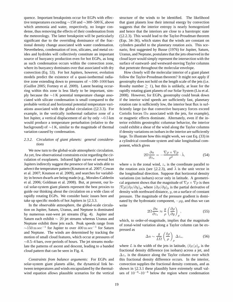
quence. Important breakpoints occur for EGPs with effec-tive temperatures exceeding∼150 and∼300–500K, abovewhich ammonia and water, respectively, no longer con-dense, thus removing the effects of their condensation fromthe meteorology. The latter breakpoint will be particularlysignificant due to the overriding dominance of the frac-tional density change associated with water condensation.Nevertheless, condensation of iron, silicates, and metal ox-ides and hydrides will collectively constitute an importantsource of buoyancy production even for hot EGPs, as longas such condensation occurs within the convection zone,where its buoyancy dominates over that associated with dryconvection (Eq. 53). For hot Jupiters, however, evolutionmodels predict the existence of a quasi-isothermal radia-tive zone extending down to pressures of∼100–1000 bars(Guillot 2005; Fortney et al. 2009). Latent heating occur-ring within this zone is less likely to be important, sim-ply because the∼1 K potential temperature change asso-ciated with silicate condensation is small compared to theprobable vertical and horizontal potential temperature vari-ations associated with the global circulation (§2.3.3). Forexample, in the vertically isothermal radiative zone of ahot Jupiter, a vertical displacement of air by only∼0.5 kmwould produce a temperature perturbation (relative to thebackground) of∼1 K, similar to the magnitude of thermalvariation caused by condensation.

2.3.2. Circulation of giant planets: general considera-tions

We now turn to the global-scale atmospheric circulation.As yet, few observational constraints exist regarding the cir-culation of exoplanets. Infrared light curves of several hotJupiters indirectly suggest the presence of fast winds abletoadvect the temperature pattern (Knutson et al. 2007; Cowanet al. 2007; Knutson et al. 2009), and searches for variabil-ity in brown dwarfs are being made (e.g., Morales-Calderonet al. 2006; Goldman et al. 2008). But, at present, our lo-cal solar-system giant planets represent the best proxies toguide our thinking about the circulation on a wide class ofrapidly rotating EGPs. We consider basic issues here andtake up specific models of hot Jupiters in§2.3.3.

In the observable atmosphere, the global-scale circula-tion on Jupiter, Saturn, Uranus, and Neptune is dominatedby numerous east-west jet streams (Fig. 4). Jupiter andSaturn each exhibit∼ 20 jet streams whereas Uranus andNeptune exhibit three jets each. Peak speeds range from∼150 m sec−1 for Jupiter to over400 m sec−1 for Saturnand Neptune. The winds are determined by tracking themotion of small cloud features, which occur at pressures of∼0.5–4 bars, over periods of hours. The jet streams modu-late the patterns of ascent and descent, leading to a bandedcloud pattern that can be seen in Fig. 4.

Constraints from balance arguments:For EGPs andsolar-system giant planets alike, the dynamical link be-tween temperatures and winds encapsulated by the thermal-wind equation allows plausible scenarios for the vertical

structure of the winds to be identified. The likelihoodthat giant planets lose their internal energy by convectionsuggests that the interior entropy is nearly homogenizedand hence that the interiors are close to a barotropic state(§2.2.3). This would lead to the Taylor-Proudman theorem(Eqs. 34–36), which states that the winds are constant oncylinders parallel to the planetary rotation axis. This sce-nario, first suggested by Busse (1976) for Jupiter, Saturn,Uranus, and Neptune, postulates that the jets observed in thecloud layer would simply represent the intersection with thesurface of eastward- and westward-moving Taylor columnsthat penetrate throughout the molecular envelope.

How closely will the molecular interior of a giant planetfollow the Taylor-Proudman theorem? It might not apply ifgeostrophy does not hold on the length scale of the jets (i.e.Rossby number& 1), but this is unlikely, at least for therapidly rotating giant planets of our Solar System (Liu et al.2008). However, for EGPs, geostrophy could break downif the interior wind speeds are sufficiently fast, planetaryrotation rate is sufficiently low, the interior heat flux is suf-ficiently large (so that convective buoyancy forces exceedCoriolis forcesΩu associated with the jets, for example),or magnetic effects dominate. Alternately, even if the in-terior exhibits geostrophic columnar behavior, the interiorcould exhibit a shear of the wind along the Taylor columnsif density variations on isobars in the interior are sufficientlylarge. To illustrate how this might work, we cast Eq. (33) ina cylindrical coordinate system and take longitudinal com-ponent, which gives

2Ω∂u

∂z∗= −∇ρ×∇p

ρ2· λ, (54)

whereu is the zonal wind,z∗ is the coordinate parallel tothe rotation axis (see§2.2.3), andλ is the unit vector inthe longitudinal direction. Suppose that horizontal densityvariations (on isobars) occur only in latitude. A geometri-cal argument shows that the magnitude of∇ρ×∇p is then|∇p|(∂ρ/∂y)p, where(∂ρ/∂y)p is the partial derivative ofdensity with northward distance,y, on a surface of constantpressure. The magnitude of the pressure gradient is domi-nated by the hydrostatic component,−ρg, and thus we canwrite

2Ω∂u

∂z∗≈ g

ρ

(

∂ρ

∂y

)

p

, (55)

which, to order-of-magnitude, implies that the magnitudeof zonal-wind variation along a Taylor column can be ex-pressed as

∆u ∼ g

LΩ

(

δρ

ρ

)

p

∆z∗, (56)

whereL is the width of the jets in latitude,(δρ/ρ)p is thefractional density difference (on isobars) across a jet, and∆z∗ is the distance along the Taylor column over whichthis fractional density difference occurs. In the interior,convection supplies the fractional density contrasts, andasshown in§2.3.1 these plausibly have extremely small val-ues of10−6–10−8 below the region where condensation

19

Fig. 4.— Left: Jupiter, Saturn, Uranus, and Neptune shown to scale in visible-wavelength images from the Cassini and Voyagerspacecraft.Right: Zonal-mean zonal wind profiles obtained from tracking small-scale cloud features over a period of hours. Jupiter andSaturn have an alternating pattern of∼ 20 east-west jets, whereas Uranus and Neptune have 3 broad jets.

can occur. We can obtain a crude order-of-magnitude es-timate for the thermal-wind shear along a Taylor columnby assuming that these fractional density differences are or-ganized on the jet scale and coherently extend across thefull ∼104 km vertical length of a Taylor column. Insertingthese values into Eq. (56), along with parameters relevant toa Jupiter-like planet (g ≈ 20 m sec−2, L ≈ 5000 km, Ω =1.74 × 10−4 sec−1) yields ∆u ∼ 0.001–0.1 m sec−1. Ifthis estimate is correct, then Jupiter-like planets would ex-hibit only small thermal-wind shear along Taylor columns,and the Taylor-Proudman theorem would hold to good ap-proximation in the molecular interior.

However, the above estimate is crude; if the jet-scalehorizontal density contrasts were much larger than the den-sity contrasts associated with convective plumes, for exam-ple, then the wind shear along Taylor columns could ex-ceed the values estimated above. The quantitative validityof Eq. (53), on which the wind-shear estimates are based,also remains uncertain. To attack the problem more rig-orously, Kaspi et al. (2009) performed full 3D numericalsimulations of convection in giant-planet interiors, suggest-ing that the compressibility may play an important role inallowing the generation of thermal-wind shear within giantplanets, especially in the outermost layers of their convec-tion zones. Such wind shear is particularly likely to be im-portant for young and/or massive planets with large interiorheat fluxes.

Although fast winds could exist throughout the molec-ular envelope, Lorentz forces probably act to brake thezonal flows in the underlying metallic region at pressuresexceeding∼1–3 Mbar (Kirk and Stevenson 1987; Groteet al. 2000; Busse 2002). The winds in the deep, metal-lic interior are thus often assumed to be weak. The transi-tion between molecular and metallic occurs gradually, andthere exists a wide semi-conducting transition zone overwhich the Taylor-Proudman theorem approximately holdsyet the electrical conductivity becomes important. Liu et al.(2008) argued that, if the observed jets on Jupiter and Sat-urn penetrated downward as Taylor columns, the Ohmicdissipation would exceed the luminosity of Jupiter (Sat-

urn) if the jets extended deeper than 95% (85%) of theplanetary radius. The observed jets are thus probably shal-lower than these depths. However, if the jets extended part-way through the molecular envelope, terminating within thesemi-conducting zone where the Ohmic dissipation occurs,the shear at the base of the jets must coexist with lateraldensity contrasts on isobars via the thermal wind relation-ship (Eq. 55). This is problematic, because, as previouslydiscussed, sufficiently large sources of density contrastsarelacking in the deep interior. Liu et al. (2008) thereforeargued that the jets must be weakthroughoutthe molecu-lar envelope up to shallow levels where alternate buoyancysources become available (e.g., latent heating and/or transi-tion to a radiative zone).

In the outermost layers of a giant planet, density varia-tions associated with latent heating and/or a transition toaradiative zone allow significant thermal wind-shear to de-velop. On Jupiter and Saturn, this so-called “baroclinic”layer begins with condensation of iron, silicates, and vari-ous metal oxides and hydrides at pressures of∼104 bars andcontinues with condensation of water, NH4SH, and ammo-nia (at∼10, 2, and 0.5 bars, respectively), finally transition-ing to the stably stratified stratosphere at∼0.2 bars. Earlymodels showed that the observed jet speeds can plausiblyresult from thermal-wind shear within this layer assumingthe winds in the interior are zero (Ingersoll and Cuzzi 1969).For example, water condensation could cause a fractionaldensity contrast on isobars of up to10−2, and if these den-sity differences extend vertically over∼100 km (roughlythe altitude difference between the water-condensation leveland the observed cloud deck), then Eq. (56) implies∆u ∼30 m sec−1, similar to the observed speed of Jupiter’s mid-latitude jets (Fig. 4).

To summarize, current understanding suggests that giantplanets should exhibit winds within the convective molecu-lar envelope that exhibit columnar structure parallel to therotation axis, transitioning in the outermost layers (pres-sures less than thousands of bars) to a baroclinic zone wherehorizontal density contrasts associated with latent heatingand/or a radiative zone allow the zonal winds to vary with

20

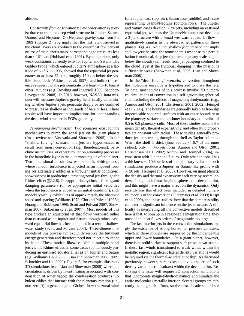
altitude.

Constraints from observations:Few observations yet ex-ist that constrain the deep wind structure in Jupiter, Saturn,Uranus, and Neptune. On Neptune, gravity data from the1989Voyager 2flyby imply that the fast jets observed inthe cloud layers are confined to the outermost few percentor less of the planet’s mass, corresponding to pressures lessthan∼105 bars (Hubbard et al. 1991). By comparison, onlyweak constraints currently exist for Jupiter and Saturn. TheGalileo Probe, which entered Jupiter’s atmosphere at a lat-itude of∼7N in 1995, showed that the equatorial jet pen-etrates to at least 22 bars, roughly150 km below the vis-ible cloud deck (Atkinson et al. 1997), and indirect infer-ences suggest that the jets penetrate to at least∼5–10 bars atother latitudes (e.g. Dowling and Ingersoll 1989; Sanchez-Lavega et al. 2008). In 2016, however, NASA’sJunomis-sion will measure Jupiter’s gravity field, finally determin-ing whether Jupiter’s jets penetrate deeply or are confinedto pressures as shallow as thousands of bars or less. Theseresults will have important implications for understandingthe deep-wind structure in EGPs generally.

Jet-pumping mechanisms:Two scenarios exist for themechanisms to pump the zonal jets on the giant planets(for a review see Vasavada and Showman 2005). In the“shallow forcing” scenario, the jets are hypothesized toresult from moist convection (e.g., thunderstorms), baro-clinic instabilities, or other turbulence-generating processesin the baroclinic layer in the outermost region of the planet.Two-dimensional and shallow-water models of this process,where random turbulence is injected as an imposed forc-ing (or alternately added as a turbulent initial condition),show success in producing alternating zonal jets through theRhines effect (§2.2.6). For appropriately chosen forcing anddamping parameters (or for appropriate initial velocitieswhen the turbulence is added as an initial condition), suchmodels typically exhibit jets of approximately the observedspeed and spacing (Williams 1978; Cho and Polvani 1996a;Huang and Robinson 1998; Scott and Polvani 2007; Show-man 2007; Sukoriansky et al. 2007). Most models of thistype produce an equatorial jet that flows westward ratherthan eastward as on Jupiter and Saturn, though robust east-ward equatorial flow has been obtained in a recent shallow-water study (Scott and Polvani 2008). Three-dimensionalmodels of this process can explicitly resolve the turbulentenergy generation and therefore need not inject turbulenceby hand. These models likewise exhibits multiple zonaljets via the Rhines effect, in some cases spontaneously pro-ducing an eastward equatorial jet as on Jupiter and Saturn(e.g. Williams 1979, 2003; Lian and Showman 2008, 2009;Schneider and Liu 2009). Figure 5, for example, illustrates3D simulations from Lian and Showman (2009) where thecirculation is driven by latent heating associated with con-densation of water vapor; the condensation produces tur-bulent eddies that interact with the planetary rotation (i.e.,non-zeroβ) to generate jets. Globes show the zonal wind

for a Jupiter case (top row), Saturn case (middle), and a caserepresenting Uranus/Neptune (bottom row). The Jupiterand Saturn cases develop∼ 20 jets, including an eastwardequatorial jet, whereas the Uranus/Neptune case developsa 3-jet structure with a broad westward equatorial flow—qualitatively similar to the observed jet patterns on theseplanets (Fig. 4). Note that shallowforcing need not implyshallowjets; because the atmosphere’s response to a pertur-bation is nonlocal, deep jets (penetrating many scale heightsbelow the clouds) can result from jet pumping confined tothe cloud layer if the frictional damping in the interior issufficiently weak (Showman et al. 2006; Lian and Show-man 2008).

In the “deep forcing” scenario, convection throughoutthe molecular envelope is hypothesized to drive the jets.To date, most studies of this process involve 3D numeri-cal simulations of convection in a self-gravitating sphericalshell excluding the effects of magnetohydrodynamics (e.g.,Aurnou and Olson 2001; Christensen 2001, 2002; Heimpelet al. 2005). The boundaries are generally taken as free-slipimpermeable spherical surfaces with an outer boundary atthe planetary surface and an inner boundary at a radius of0.5 to 0.9 planetary radii. Most of these studies assume themean density, thermal expansitivity, and other fluid proper-ties are constant with radius. These studies generally pro-duce jets penetrating through the shell as Taylor columns.When the shell is thick (inner radius≤ 0.7 of the outerradius), only∼ 3–5 jets form (Aurnou and Olson 2001;Christensen 2001, 2002; Aurnou and Heimpel 2004), in-consistent with Jupiter and Saturn. Only when the shell hasa thickness∼ 10% or less of the planetary radius do suchsimulations produce a Jupiter- or Saturn-like profile with∼ 20 jets (Heimpel et al. 2005). However, on giant planets,the density and thermal expansivity each vary by several or-ders of magnitude from the photosphere to the deep interior,and this might have a major effect on the dynamics. Onlyrecently has this effect been included in detailed numeri-cal models of the convection (Glatzmaier et al. 2009; Kaspiet al. 2009), and these studies show that the compressibilitycan exert a significant influence on the jet structure. A dif-ficulty in interpreting all the convective models describedhere is that, to spin up in a reasonable integration time, theymust adopt heat fluxes orders of magnitude too large.

The fast interior jets in these convection simulations im-ply the existence of strong horizontal pressure contrasts,which in these models are supported by the impermeableupper and lower boundaries. On a giant planet, however,there is no solid surface to support such pressure variations.If these fast winds transitioned to weak winds within themetallic region, significant lateral density variations wouldbe required via the thermal-wind relationship. As discussedpreviously, however, there exists no obvious source of suchdensity variations (on isobars) within the deep interior. Re-solving this issue will require 3D convection simulationsthat incorporate magnetohydrodynamics and simulate theentire molecular+metallic interior. Several groups are cur-rently making such efforts, so the next decade should see

21

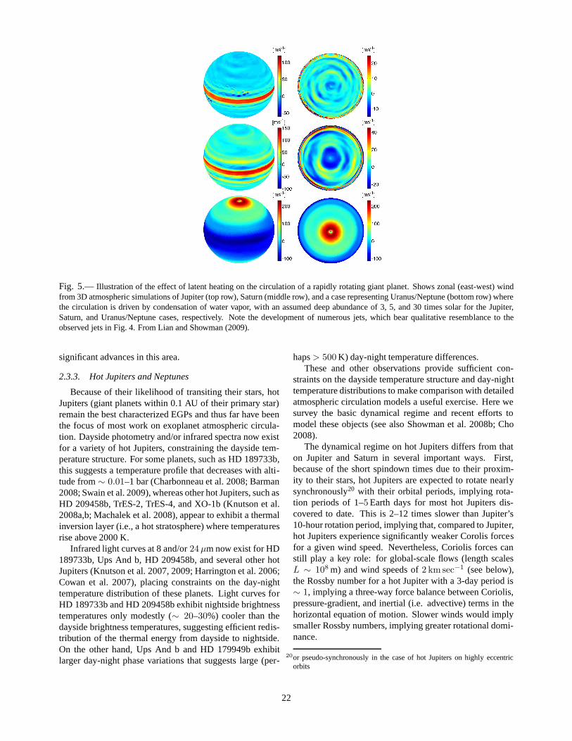
Fig. 5.— Illustration of the effect of latent heating on the circulation of a rapidly rotating giant planet. Shows zonal (east-west) windfrom 3D atmospheric simulations of Jupiter (top row), Saturn (middle row), and a case representing Uranus/Neptune (bottom row) wherethe circulation is driven by condensation of water vapor, with an assumed deep abundance of 3, 5, and 30 times solar for theJupiter,Saturn, and Uranus/Neptune cases, respectively. Note the development of numerous jets, which bear qualitative resemblance to theobserved jets in Fig. 4. From Lian and Showman (2009).

significant advances in this area.

2.3.3. Hot Jupiters and Neptunes

Because of their likelihood of transiting their stars, hotJupiters (giant planets within 0.1 AU of their primary star)remain the best characterized EGPs and thus far have beenthe focus of most work on exoplanet atmospheric circula-tion. Dayside photometry and/or infrared spectra now existfor a variety of hot Jupiters, constraining the dayside tem-perature structure. For some planets, such as HD 189733b,this suggests a temperature profile that decreases with alti-tude from∼ 0.01–1 bar (Charbonneau et al. 2008; Barman2008; Swain et al. 2009), whereas other hot Jupiters, such asHD 209458b, TrES-2, TrES-4, and XO-1b (Knutson et al.2008a,b; Machalek et al. 2008), appear to exhibit a thermalinversion layer (i.e., a hot stratosphere) where temperaturesrise above 2000 K.

Infrared light curves at 8 and/or24µm now exist for HD189733b, Ups And b, HD 209458b, and several other hotJupiters (Knutson et al. 2007, 2009; Harrington et al. 2006;Cowan et al. 2007), placing constraints on the day-nighttemperature distribution of these planets. Light curves forHD 189733b and HD 209458b exhibit nightside brightnesstemperatures only modestly (∼ 20–30%) cooler than thedayside brightness temperatures, suggesting efficient redis-tribution of the thermal energy from dayside to nightside.On the other hand, Ups And b and HD 179949b exhibitlarger day-night phase variations that suggests large (per-

haps> 500 K) day-night temperature differences.These and other observations provide sufficient con-

straints on the dayside temperature structure and day-nighttemperature distributions to make comparison with detailedatmospheric circulation models a useful exercise. Here wesurvey the basic dynamical regime and recent efforts tomodel these objects (see also Showman et al. 2008b; Cho2008).

The dynamical regime on hot Jupiters differs from thaton Jupiter and Saturn in several important ways. First,because of the short spindown times due to their proxim-ity to their stars, hot Jupiters are expected to rotate nearlysynchronously20 with their orbital periods, implying rota-tion periods of 1–5 Earth days for most hot Jupiters dis-covered to date. This is 2–12 times slower than Jupiter’s10-hour rotation period, implying that, compared to Jupiter,hot Jupiters experience significantly weaker Corolis forcesfor a given wind speed. Nevertheless, Coriolis forces canstill play a key role: for global-scale flows (length scalesL ∼ 108 m) and wind speeds of2 km sec−1 (see below),the Rossby number for a hot Jupiter with a 3-day period is∼ 1, implying a three-way force balance between Coriolis,pressure-gradient, and inertial (i.e. advective) terms inthehorizontal equation of motion. Slower winds would implysmaller Rossby numbers, implying greater rotational domi-nance.

20or pseudo-synchronously in the case of hot Jupiters on highly eccentricorbits

22

Second, hot Jupiters receive enormous energy fluxes(∼ 104–106 W m−2 on a global average) from their parentstars, in contrast to the∼ 10 Wm−2 received by Jupiterand 1 W m−2 for Neptune. The resulting high tempera-tures lead to short radiative time constants of days or lessat pressures< 1 bar (Showman and Guillot 2002; Iro et al.2005; Showman et al. 2008a, and Eq. (28)), in contrast toJupiter where radiative time constants are years. Even in thepresence of fast winds, these short radiative time constantsallow the possibility of large fractional day-night tempera-ture differences, particularly on the most heavily irradiatedplanets—in contrast to Jupiter where temperatures vary hor-izontally by only a few percent.

Third, over several Gyr of evolution, the intense irradi-ation received by hot Jupiters leads to the development ofa nearly isothermal radiative zone extending to pressures of∼ 100–1000 bars (Guillot et al. 1996; Guillot 2005; Fort-ney et al. 2009). The observable weather in hot Jupiters thusoccurs not within the convection zone but within the stablystratified radiative zone. Moreover, as described in§2.3.1,this separation between the photosphere and the radiative-convective boundary may allow large horizontal tempera-ture differences to develop and support significant thermal-wind shear. For example, assuming that a lateral tempera-ture contrast of∆T ∼ 300 K extending over several scaleheights (∆ln p ∼ 3) occurs over a lateral distance of108 m,the resulting thermal-wind shear∆u ∼ 2 km sec−1. Thus,balance arguments suggest that the existence of significanthorizontal temperature contrasts would naturally requirefast wind speeds.

The modest rotation rates, large stable stratifications, andpossible fast wind speeds suggest that the Rossby defor-mation radius and Rhines scale are large on hot Jupiters.On Jupiter, the deformation radius is∼ 2000 km and theRhines scale is∼ 104 km (much smaller than the planetaryradius of71, 400 km), which helps explain why Jupiter andSaturn have an abundant population of small vortices andnumerous zonal jets (Figs. 3–4) (Williams 1978; Cho andPolvani 1996a; Vasavada and Showman 2005). In contrast,a hot Jupiter with a rotation period of 3 Earth days and windspeed of2 km sec−1 has a deformation radius and Rhinesscale comparable to the planetary radius. Thus, dynamicalstructures such as vortices and jets should be more global inscale than occurs on Jupiter and Saturn (Menou et al. 2003;Showman and Guillot 2002; Cho et al. 2003). This scal-ing argument is supported by detailed nonlinear numericalsimulations of the circulation, which generally show the de-velopment of only∼ 1–3 broad jets (Showman and Guillot2002; Cho et al. 2003, 2008; Dobbs-Dixon and Lin 2008;Langton and Laughlin 2007, 2008a; Showman et al. 2008a,2009).

A variety of 2D and 3D models have been used to inves-tigate the atmospheric circulation of hot Jupiters. Cho et al.(2003, 2008) performed global numerical simulations of hotJupiters on circular orbits using the one-layer equivalentbarotropic equations (Eq. 8). They initialized the simula-tions with small-scale balanced turbulence and forced them

with a large-scale deflection of the lower bounding surface(see§2.1.3) to provide a crude representation of the pressureeffects of the day-night heating gradient. However, no ex-plicit heating/cooling was included. Together, these effectsled to the production of several broad, meandering jets anddrifting polar vortices. The mean wind speed in the finalstate is to a large degree determined by the mean speed ofthe initial turbulence, which ranged from100–800 m sec−1

in their models. At the large (∼planetary-scale) deforma-tion radius relevant to hot Jupiters, the equatorial jet in thefinal state can flow either eastward or westward depend-ing on the initial condition and other details. The simu-lations exhibit significant time variability that, if present onhot Jupiters, would lead to detectable orbit-to-orbit variabil-ity in light curves and secondary eclipse depths (Cho et al.2003; Rauscher et al. 2007, 2008).

Langton and Laughlin (2007) performed global, 2D sim-ulations of hot Jupiters on circular orbits using the shallow-water equations with a mass source on the dayside andmass sink on the nightside to parameterize the effects ofdayside heating and nightside cooling. When the obliq-uity is assumed zero and the mass sources/sinks are suffi-ciently large, their forced flows quickly reach a steady statewith wind speeds of∼ 1 km sec−1 and order-unity lateralvariations in the thickness of the shallow-water layer. Onthe other hand, Langton and Laughlin (2008a) numericallysolved the 2D fully compressible equations for the horizon-tal velocity and temperature of hot Jupiters on eccentric or-bits and obtained very turbulent, time-varying flows. Ap-parently, in this case, the large-scale heating patterns pro-duced hemisphere-scale vortices that were dynamically un-stable, leading to the breakdown of these eddies into small-scale turbulence.

Several authors have also performed 3D numerical sim-ulations of hot Jupiters. Showman and Guillot (2002),Cooper and Showman (2005, 2006), Showman et al.(2008a), and Menou and Rauscher (2009) performed globalsimulations with the 3D primitive equations where the day-side heating and nightside cooling was parameterized with aNewtonian heating/cooling scheme, which relaxes the tem-peratures toward a prescribed radiative-equilibrium tem-perature profile (hot on the dayside, cold on the nightside)over a prescribed radiative timescale. Dobbs-Dixon and Lin(2008) performed simulations with the fully compressibleequations in a limited-area domain, consisting of the equa-torial and mid-latitudes but with the poles cut off. Like thestudies listed above, they also adopted a simplified methodfor forcing their flow, in this case using a radiative diffusionscheme. Showman et al. (2009) coupled their global 3Ddynamical solver to a state-of-the-art, non-gray, cloud-freeradiative transfer scheme with opacities calculated assum-ing local chemical equilibrium (Figs. 7 and 8). The abovemodels models all generally obtain wind structures with∼ 1–3 broad jets with speeds of∼ 1–4 km sec−1.

Despite the diversity in modeling approaches, the studiesdescribed above agree in several key areas.

23

-90

-60

-30

0

30

60

90

-400 -200 0 200 400

Latit

ude

[deg

]

Eastward Velocity [m/s]

Fig. 6.— One-layer, global equivalent barotropic simulation of thehot Jupiter HD 209458b from Cho et al. (2003). Globes showequatorial (left) and polar (right) views of the potential vorticity (Eq. 12); note the development of large polar vortices and small-scaleturbulent structure, which result from a combination of theturbulent initial condition and large-scale “topographic” forcing intended toqualitatively represent the day-night heating contrast. Plot shows zonal-mean zonal wind versus latitude, illustrating the 3-jet structurethat develops.

Fig. 7.— Results from a 3D simulation of the hot Jupiter HD 189733b from Showman et al. (2009). The dynamics are coupled toa realistic representation of cloud-free, non-gray radiative transfer assuming solar abundances.Left: Temperature (colorscale, in K)and winds (arrows) at the 30 mbar pressure, which is the approximate level of the mid-IR photosphere. A strong eastward equatorialjet develops that displaces the hottest regions eastward from the substellar point (which lies at0

longitude,0 latitude). Right: Lightcurves inSpitzerbandpasses calculated from the simulation (curves; labelsshow wavelength inµm) in comparison to observations(points) from Knutson et al. (2007, 2009), Charbonneau et al. (2008), and Deming et al. (2006).

24

Fig. 8.— 3D simulation of HD 209458b, including realistic cloud-free, non-gray radiative transfer, illustrating developmentof adayside stratosphere when opacity from visible-absorbingspecies (in this case TiO and VO) are included. Such stratospheres arerelevant to explainingSpitzerdata of HD 209458b, TrES-2, TrES-4, XO-1b, and other hot Jupiters. Here, the stratosphere (shown inred) begins at pressures of∼ 10 mbar and widens with altitude until it covers most of the dayside at pressures of∼ 0.1 mbar. Panelsshow temperature (colorscale, in K) and winds (arrows) at the 0.08, 1, and 30 mbar levels from top to bottom, respectively. Substellarlongitude and latitude are (0

, 0). From Showman et al. (2009).

25

• First, most of the above studies generally producepeak wind speeds similar to within a factor of 2–3, in the range of one to severalkm sec−1.21 Thissimilarity is not a coincidence but results from theforce balances that occur for a global-scale flow inthe presence of large fractional temperature differ-ences. Consider the longitudinal force balance at theequator, for example, and suppose the day-night heat-ing gradient produces a day-night temperature differ-ence∆Thoriz that extends vertically over a range oflog-pressures∆log p. This temperature differencecauses a day-night horizontal pressure-gradient ac-celeration which, to order-of-magnitude, can be writ-tenR∆Thoriz∆log p/a, wherea is the planetary ra-dius. At high latitudes, this could be balanced by theCoriolis force arising from a north-south flow, but thehorizontal Coriolis force is zero at the equator. At theequator, such a force instead tends to cause accelera-tion of the flow in the east-west direction. Balancingthe pressure-gradient acceleration byv·∇v, which toorder-of-magnitude isU2/a for a global-scale flow,we have

U ∼√

R∆Thoriz∆ln p (57)

This should be interpreted as the characteristic vari-ation in zonal wind speed along the equator. ForR = 3700 J kg−1 K−1, ∆Thoriz ∼ 400 K, and∆ln p ∼ 3 (appropriate to a temperature differenceextending vertically over three scale heights), thisyieldsU ∼ 2 km sec−1.

Likewise, consider the latitudinal force balance inthe mid-latitudes. To order-of-magnitude, the lati-tudinal pressure-gradient acceleration is again givenbyR∆Thoriz∆ln p/a, where here∆Thoriz is the lat-itudinal temperature contrast (e.g., from equator topole) that extends vertically over∆ln p. If Ro ≫ 1,this is balanced by the advective accelerationU2/a,whereas ifRo ≪ 1, it would instead be balanced bythe Coriolis accelerationfU , wheref is the Cori-olis parameter (§2.2.3). The former case recoversEq. (57), whereas the latter case yields

U ∼ R∆Thoriz∆ln p

fa(58)

Here,U is properly interpreted as the characteristicdifference in horizontal wind speed vertically across∆ln p. InsertingR = 3700 J kg−1 K−1, ∆Thoriz ∼400 K, ∆ln p ∼ 3, f ∼ 2 × 10−5 (appropriate inmid-latitudes to a hot Jupiter with a 3-day period),anda ≈ 108 m, we again obtainU ∼ 2 km sec−1. 22

21In intercomparing studies, one must be careful to distinguish mean versuspeak speeds and, in the case of 3D models, the pressure level at whichthose speeds are quoted; such quantities can differ by a factor of several ina single model.

22The similarity of the numerical estimates from Eq. (57) and (58) resultsfrom the fact that we assumed the same horizontal temperature differencesin longitude and latitude and thatRo ∼ 1 for the parameter regime ex-plored here.

While not minimizing the real differences in the nu-merical results obtained in the various studies, theabove estimates show that the existence of windspeeds of a fewkm sec−1 in the various numericalstudies is a basic outcome of force balance in thepresence of lateral temperature contrasts of hundredsof K.

• Second, the various numerical studies all produce asmall number (∼ 1–4) of broad jets. This was firstpointed out by Showman and Guillot (2002), Menouet al. (2003), and Cho et al. (2003) and, as describedpreviously, results from the fact that the Rossby de-formation radius and Rhines scale are comparable toa planetary radius for typical conditions relevant tohot Jupiters. Follow-up studies have confirmed thesegeneral expectations (Cooper and Showman 2005;Cho et al. 2008; Langton and Laughlin 2007, 2008a;Dobbs-Dixon and Lin 2008; Showman et al. 2008a,2009).

Despite these similarities, there remain some key dif-ferences in the numerical results obtained by the variousgroups so far. These include the following:

• As yet, little agreement exists on whether hot Jupitersshould exhibit significant temporal variability on theglobal scale. The 2D simulations of Cho et al. (2003,2008) and Langton and Laughlin (2008a) producehighly turbulent, time-variable flows, whereas theshallow-water study of Langton and Laughlin (2007)and most of the 3D studies (Showman and Guillot2002; Cooper and Showman 2005; Dobbs-Dixon andLin 2008; Showman et al. 2008a, 2009) exhibit rel-atively steady flow patterns with only modest timevariability for zero-obliquity, zero-eccentricity hotJupiters. The Cho et al. simulations essentially guar-antee a time-variable outcome because of the tur-bulent initial condition, although breaking Rossbywaves and dynamical instabilities during the simula-tions also play a large role; the Langton and Laugh-lin (2008a) simulations were initialized from rest andnaturally develop turbulence via dynamical instabil-ity throughout the course of the simulation.

Time variability can result from several mechanisms,including dynamical (e.g., barotropic or baroclinic)instabilities, large-scale oscillations, and modifica-tion of the jet pattern by atmospheric waves. Ifthe jet pattern is dynamically stable (or, more rig-orously, if relevant instability growth times are sig-nificantly longer than the characteristic atmosphericheating/cooling times), then this mechanism for pro-ducing variability would be inhibited; on the otherhand, if the jet pattern is unstable (with instabilitygrowth rates comparable to or less than the heat-ing/cooling times), the jets will naturally break upand produce a wide range of turbulent eddies. In thisregard, it is crucial to carefully distinguish between

26

2D and 3D models, because they exhibit very dif-ferent stability criteria (e.g., Dowling 1995). For ex-ample, in a 2D, nondivergent model, theoretical andnumerical work shows that jets are guaranteed stableonly if

∂2u

∂y2< β (59)

a relationship called thebarotropic stability criterion.Numerical simulations show that 2D, nondivergentfluids initialized with jets violating Eq. (59) gener-ally develop instabilities that rob energy from the jetsuntil the jets no longer violate the equation. However,jets in a 3D fluid can in some cases strongly violateEq. (59) while remaining stable; Jupiter and Saturn,for example, have several jets where∂2u/∂y2 exceedβ by a factor of 2–3 (Ingersoll et al. 1981; Sanchez-Lavega et al. 2000), and yet the jet pattern has re-mained almost unchanged over multi-decade timescales. This may simply imply that the barotropicstability criterion is irrelevant for a 3D fluid (Dowl-ing 1995; Vasavada and Showman 2005). Thus, it isa priori unsurprising that 2D and 3D models wouldmake different predictions for time variability. Acareful study of the conditions under which time vari-ability can occur for hot Jupiters should thereforeadopt 3D models—or, at a minimum, 2D modelswith a finite Rossby deformation radius (such as theshallow-water or equivalent-barotropic model).

However, a recent study by Menou and Rauscher(2009) shows that the issue is not only one of 2Dversus 3D. Making straightforward extensions to anEarth model, they performed forced 3D shallow sim-ulations initialized from rest that developed highlyturbulent, time variable flows on the global scale,showing that time variability from the emergence ofhorizontal shear instability may occur in 3D undersome conditions relevant to hot Jupiters. Like sev-eral previous studies, they forced their flows with aNewtonian heating/cooling scheme that generates aday-night temperature difference. However, a care-ful comparison shows that their forcing set-up differssignificantly from those of previous studies. Theyplace an impermeable surface at 1 bar and apply theirmaximum day/night forcing immediately above thesurface; the day-night radiative-equilibrium temper-ature difference decreases with altitude and reacheszero near the top of their model. This is backwardsfrom the set-up used in Cooper and Showman (2005,2006) and Showman et al. (2008a, 2009) where theforcing amplitude peaks near the top of the domainand decreases with depth, and where the surface isplaced significantly deeper than the region of atmo-spheric heating/cooling to minimize its interactionwith the circulation in the observable atmosphere.The differences in the forcing schemes and positionof the surface presumably determine whether or not a

given 3D simulation develops global-scale instabilityand time variability. Further work will be necessaryto identify the specific forcing conditions that lead totime-variable or quasi-steady conditions at the globalscale.

It is also worth remembering that hot Jupiters them-selves exhibit huge diversity; among the known tran-siting planets, for example, incident stellar flux variesby a factor of∼ 150, gravities range over a factor of∼ 70, and expected rotation rates vary over nearlya factor of 10 (e.g., Table 1). Given this diversity,it is reasonable to expect that some hot Jupiters willexhibit time-variable conditions while others will ex-hibit relatively steady flow patterns.

• Another area of difference between models regardsthe direction of the equatorial jet. The shallow-waterand equivalent barotropic models can produce ei-ther eastward or westward equatorial jets, depend-ing on the initial conditions and other modeling de-tails (Cho et al. 2003, 2008; Langton and Laughlin2007, 2008a). In contrast, all of the 3D models pub-lished to date for synchronously rotating hot Jupiterswith zero obliquity and eccentricity have producedrobust eastward equatorial jets (Showman and Guil-lot 2002; Cooper and Showman 2005, 2006; Show-man et al. 2008a, 2009; Dobbs-Dixon and Lin 2008;Menou and Rauscher 2009). The mechanisms re-sponsible for generating the eastward jets in these 3Dmodels remain to be diagnosed in detail but presum-ably involve the global-scale eddies generated by theday-night heating contrast.

To date, most work on hot-Jupiter atmospheric circula-tion has emphasized planets on circular orbits. However,several transiting hot Jupiters and Neptunes have eccentricorbits, including GJ 436b, HAT-P-2b, HD 17156b, and HD80606b, whose orbital eccentricities are 0.15, 0.5, 0.67, and0.93, respectively. When the eccentricity is large, the inci-dent stellar flux varies significantly throughout the orbit—HAT-P-2b, for example, receives∼ 9 times more flux at pe-riapse than at apoapse, while for HD 80606b, the maximumincident flux exceeds the minimum incident flux by a fac-tor of over 800! These variations dwarf those experiencedin our Solar System and constitute an uncharted regime ofdynamical forcing for a planetary atmosphere. An 8-µmlight curve of HD 80606b has recently been obtained withthe Spitzer Space Telescopeduring a 30-hour interval sur-rounding periapse passage (Laughlin et al. 2009), whichshows the increase in planetary flux that presumably ac-companies the flash heating as the planet passes by its star.2D and 3D numerical simulations suggest that these plan-ets may exhibit dynamic, time-variable flows and show thatthe planet’s emitted infrared flux can peak hours to days af-ter periapse passage (Langton and Laughlin 2008a,b; Lewiset al. 2009).

27

2.3.4. Chemistry as a probe of the meteorology

Chemistry can provide important constraints on the me-teorology of giant planets. On Jupiter, for example, gaseousCO, PH3, GeH4, and AsH3 have been detected in the uppertroposphere (p < 5 bars) with mole fractions of∼ 0.8, 0.2,0.6, and 0.5–1 ppb, respectively. None of these compoundsare thermochemically stable in the upper troposphere—thechemical equilibrium mole fractions are< 10−14 for AsH3

and< 10−20 for the other three species (Fegley and Lod-ders 1994). However, the equilibrium abundances of allfour species rise with depth, exceeding 1 ppb at pressuresgreater than 500, 400, 160, and 20 bars for CO, PH3, GeH4,and AsH3, respectively. Thus, the high abundances of thesespecies in the upper troposphere appear to result from rapidconvective mixing from the deep atmosphere.23 Kinetic re-action times are rapid at depth but plummet with decreasingtemperature and pressure, allowing these species to persistin disequilibrium (i.e., “quench”) in the low-pressure andtemperature conditions of the upper troposphere. Knowl-edge of the chemical kinetic rate constants allows quantita-tive estimates to be made of the vertical mixing rate neededto explain the observed abundances. For all four of thespecies listed above, the required vertical mixing rates yieldorder-of-magnitude matches with the mixing rate expectedfrom thermal convection at Jupiter’s known heat flux (e.g.Prinn and Barshay 1977; Fegley and Lodders 1994; Bezardet al. 2002). Thus, the existence of these disequilibriumspecies provides evidence that the deep atmosphere is in-deed convective.

Given the difficulty of characterizing the meteorologyof EGPs with spatially resolved observations, these typesof chemical constraints will likely play an even more im-portant role in our understanding of EGPs than is the casefor Jupiter. Several brown dwarfs, including Gl 229b, Gl570d, and 2MASS J0415-0935, show evidence for dise-quilibrium abundances of CO and/or NH3 (e.g., Noll et al.1997; Saumon et al. 2000, 2006, 2007). These observationscan also plausibly be explained by vertical mixing. Forthese objects, NH3 is quenched in the convection zone, butCO is quenched in the overlying radiative zone where ver-tical mixing must result from some combination of small-scale turbulence (due, for example, to the breaking of verti-cally propagating gravity waves) and vertical advection dueto the large-scale circulation (§2.2.7). Current models sug-gest that such mixing corresponds to an eddy diffusivity inthe radiative zone of∼ 1–10 m2 sec−1 for Gl 229b and10–100 m2 sec−1 for 2MASS J0415-0935 (Saumon et al.2007). These inferences on vertical mixing rate provideconstraints on the atmospheric circulation that would be dif-ficult to obtain in any other way.

Several hot Jupiters likewise reside in temperatureregimes where CH4 is the stable form in the observableatmosphere and CO is the stable form at depth, or where

23Jupiter also has a high stratospheric CO abundance that is inferred to resultfrom exogenous sources (Bezard et al. 2002).

CH4 is the stable form on the nightside and CO is the stableform on the dayside. The abundance and spatial distributionof CO and CH4 on these objects could thus provide impor-tant clues about the wind speeds and other aspects of themeteorology. CH4 has been detected via transmission spec-troscopy on HD 189733b (Swain et al. 2008) and CO hasbeen indirectly inferred from the shape of the dayside emis-sion spectrum (Barman 2008), although further observa-tions and radiative-transfer models are needed to determinetheir abundances and spatial variability (if any). Cooperand Showman (2006) coupled a simple model for CO/CH4

interconversion kinetics to their 3D dynamical model ofhot Jupiters to demonstrate that CO and CH4 should bequenched in the observable atmosphere, where thermo-chemical CO↔CH4 interconversion times are orders ofmagnitude longer than plausible dynamical times. If so, onewould expect CO and CH4 to have similar abundances onthe dayside and nightside of hot Jupiters, in contrast to thechemical-equilibrium situation where CH4 would be muchmore prevalent on the nightside (note, however, that theirmodels neglect photochemistry, which could further modifythe abundances of both species). For temperatures relevantto objects like HD 209458b and HD 189733b, Cooper andShowman (2006) found that the quenching occurs at pres-sures of∼ 1–10 bars, and that the quenched abundancedepends primarily on the temperatures and vertical veloci-ties in this pressure range.

Thus, future observational determination of CO and CH4

abundances and comparison with detailed 3D models mayallow constraints on the temperatures and vertical veloci-ties in the deep (1–10 bar) atmospheres of hot Jupiters tobe obtained. Such constraints probe significantly deeperthan the expected visible and infrared photospheres of hotJupiters and hence would nicely complement the charac-terization of hot-Jupiter thermal structure via light curvesand secondary-eclipse spectra. Note also that an analogousstory involving N2 and NH3 interconversion may occur oneven cooler objects (Teff ∼ 700 K “warm” Jupiters).

2.4. Circulation regimes: terrestrial planets

With current groundbased searches and upcoming space-craft such as NASA’sKeplermission, terrestrial planets arelikely to be discovered around main-sequence stars withinthe next five years, and basic characterization of their atmo-spheric composition and temperature structure should fol-low over the subsequent decade. At base, we wish to un-derstand not only whether such planets exist but whetherthey have atmospheres, what their atmospheric composi-tion, structure and climate may be, and whether they cansupport life. Addressing these issues will require a consid-eration of relevant physical and chemical climate feedbacksas well as the plausible circulation regimes in these planets’atmospheres.

The study of extrasolar terrestrial planet atmospheres isjust beginning, and only a handful of papers have specifi-cally investigated the possible circulation regimes on these

28

objects. However, a vast literature has developed to under-stand the climate and circulation of Venus, Titan, Mars, andespecially Earth, and many of the insights developed for un-derstanding these planets may be generalizable to exoplan-ets. Our goal here is to provide conceptual and theoreticalguidance on the types of climate and circulation processesthat exist in terrestrial planet atmospheres and discuss howthose processes vary under diverse planetary conditions. In§2.4.1 we survey basic issues in climate. The followingsections,§2.4.3–§2.4.5, address basic circulation regimeson terrestrial planets, emphasizing those aspects (e.g., pro-cesses that determine the horizontal temperature contrasts)relevant to future exoplanet observations.§2.4.6 discussesregimes of exotic forcing associated with synchronous ro-tation, large obliquities, and large orbital eccentricities.

2.4.1. Climate

Climate can be defined as the mean condition of aplanet’s atmosphere/ocean system—the temperatures, pres-sures, winds, humidities, and cloud properties—averagedover time intervals longer than the timescale of typicalweather events. The climate on the terrestrial planets re-sults from a wealth of interacting physical, chemical, ge-ological, and (when relevant) biological effects, and evenon Earth, understanding the past and present climate hasrequired a multi-decade interdisciplinary research effort. Inthis section, we provide only a brief sampling of the sub-ject, touching only on the most basic physical processesthat help to determine a planet’s global-mean conditions.

The mean temperatures at which a planet radiates tospace depends primarily on the incident stellar flux andthe planetary albedo. Equating emitted infrared energy(assumed blackbody) with absorbed stellar flux yieldsa planet’s global-mean effective temperature at radiativeequilibrium:

Teff =

[

F⋆(1 −Ab)

4σ

]1/4

(60)

whereF⋆ is the incident stellar flux,Ab is the planet’sglobal-mean bond albedo24, andσ is the Stefan-Boltzmannconstant. The factor of 4 results from the fact that the planetintercepts a stellar beam of areaπa2 but radiates infraredfrom its full surface area of4πa2.

Given an incident stellar flux, a variety of atmosphericprocesses act to determine the planet’s surface temperature.First, the circulation and various atmospheric feedbacks canplay a key role in determining the planetary albedo. Barerock is fairly dark, and for terrestrials planet the albedo islargely determined by the distribution of clouds and surfaceice. The Moon, for example, has bond albedo of 0.11, yield-ing an effective temperature of274 K. In contrast, Venushas a bond albedo of 0.75 because of its global cloud cover,yielding an effective temperature of232 K. With partial

24The bond albedo is the fraction of light incident upon a planet that is scat-tered back to space, integrated over all wavelengths and directions.

cloud and ice cover, Earth is an intermediate case, with abond albedo of 0.31 and an effective temperature of255 K.These examples illustrate that the circulation, via its effecton clouds and surface ice, can have a major influence onmean conditions—Venus’ effective temperature is less thanthat of the Earth and Moon despite receiving nearly doublethe Solar flux!

Second,Teff is not the surface temperature but themean blackbody temperature at which the planet radiatesto space. The surface temperatures can significantly exceedTeff through thegreenhouse effect.Planets orbiting Sun-like stars receive most of their energy in the visible, butthey tend to radiate their energy to space in the infrared.Most gases tend to be relatively transparent in the visible,but H2O, CO2, CH4, and other molecules absorb signif-icantly in the infrared. On a planet like Earth or Venus,a substantial fraction of the sunlight therefore reaches theplanetary surface, but infrared emission from the surfaceis mostly absorbed in the atmosphere and cannot radiatedirectly to space. In turn, the atmosphere radiates both up(to space) and down (to the surface). The surface thereforereceives a double whammy of radiation from both the Sunand the atmosphere; to achieve energy balance, the surfacetemperature becomes elevated relative to the effective tem-perature. This is the greenhouse effect. Contrary to populardescriptions, the greenhouse effect shouldnot be thoughtof as a situation where the heat is “trapped” or “cannotescape.” Indeed, the planet as a whole resides in a near-balance where infrared emission to space (mostly from theatmosphere when the greenhouse effect is strong) almostequals absorbed sunlight.

To have a significant greenhouse effect, a planet musthave a massive-enough atmosphere to experience pressurebroadening of the spectral lines. Mars, for example, has∼ 15 times more CO2 per area than Earth, yet its green-house effect is significantly weaker because its surface pres-sure is only 6 mbar.

The climate is influenced by numerous feedbacks thatcan affect the mean state and how the atmosphere respondsto perburbations. Some of the more important feedbacksare as follows:

• Thermal feedback:Increases or decreases in the tem-perature at the infrared photosphere lead to enhancedor reduced radiation to space, respectively. This is anegative feeback that allows planets to reach a stableequilibrium with absorbed starlight.

• Ice-albedo feedback:Surface ice can form on plan-ets exhibiting trace gases that can condense to solidform. Because of the brightness of ice and snow, anincrease in snow/ice coverage decreases the absorbedstarlight, promoting colder conditions and growth ofeven more ice. Conversely, melting of surface iceincreases the absorbed starlight, promoting warmerconditions and continued melting. This is a positivefeedback.

29

Simple models of the ice-albedo feedback show that,over a range ofF⋆ values (depending on the strengthof the greenhouse effect), an Earth-like planet can ex-hibit two stable equilibrium states for a given valueof F⋆: a warm, ice-poor state with a low albedo anda cold, ice-covered state with a high albedo (e.g.,North et al. 1981). Geologic evidence suggests that∼ 0.6–2.4 Gyr ago Earth experienced several multi-Myr-long glaciations with global or near-global icecover (dubbed “snowball Earth” events; Hoffman andSchrag 2002), suggesting that Earth has flipped backand forth between these equilibria. The susceptibilityof a planet to entering such a snowball state is highlysensitive to the strength of latitudinal heat transport(Spiegel et al. 2008), thereby linking this feedback tothe global circulation.

• Condensable-greenhouse-gas feedback:When an at-mospheric constituent is a greenhouse gas that alsoexists in condensed form on the surface, the atmo-sphere can experience a positive feedback that af-fects the temperature and the distribution of this con-stituent between the atmosphere and surface. Anincrease in surface temperature increases the con-stituent’s saturation vapor pressure, hence the evapo-ration rate, the atmospheric abundance and thereforethe greenhouse effect. A decrease in surface temper-ature decreases the saturation vapor pressure, reduc-ing the evaporation rate, the atmospheric abundance,and therefore the greenhouse effect. Thermal pertur-bations are therefore amplified. For Earth, this pro-cess occurs with water vapor (Earth’s most impor-tant greenhouse gas) and is called the “water-vaporfeedback” in the Earth climate literature (Held andSoden 2000). The water-vapor feedback will play amajor role in determining how Earth responds to an-thropogenic increases in carbon dioxide over the nextcentury.

In some circumstances, this positive feedback isso strong that it can trigger a runaway that shiftsthe atmosphere into a drastically different state. Inthe case of warming, this would constitute arun-away greenhousethat leads to the complete evapora-tion/sublimation of the condensable constituent fromthe surface. If early Venus had oceans, for example,they might have experienced runaway evaporation,leading to a monstrous early water vapor atmosphere(Ingersoll 1969; Kasting 1988) that would have hadmajor effects on subsequent planetary evolution.

In the case of cooling, such a runaway would removemost of the condensable constituent from the atmo-sphere, and if the relevant gas dominates the atmo-sphere, this could lead toatmospheric collapse. Forexample, if a Venus-like planet (with its∼ 500-Kgreenhouse effect) were moved sufficiently far fromthe Sun, CO2 condensation would initiate, potentiallycollapsing the atmosphere to a Mars-like state with

most of the CO2 condensed on the ground, a cold,thin CO2 atmosphere in vapor-pressure equilibriumwith the surface ice, and minimal greenhouse effect.The CO2 cloud formation that precedes such a col-lapse is often used to define the outer edge of theclassical habitable zone for terrestrial planets whosegreenhouse effect comes primarily from CO2 (Kast-ing et al. 1993).

Because CO2 condensation naturally initiates inthe coldest regions (the poles for a rapidly rotatingplanet; the nightside for a synchronous rotator), theconditions under which atmospheric collapse initi-ates depend on the atmospheric circulation. Weakequator-to-pole (or day-night) heat transport leads tocolder polar (or nightside) temperatures for a givensolar flux, promoting atmospheric collapse. Thesedynamical effects have yet to be fully included inclimate models.

• Clouds:Cloud coverage increases the albedo, lessen-ing the absorption of starlight and promoting coolerconditions. On the other hand, because the tro-pospheric temperatures generally decrease with alti-tude, cloud tops are typically cooler than the groundand therefore radiate less infrared energy to space,promoting warmer conditions (an effect that dependssensitively on cloud altitude and latitude). These ef-fects compete with each other. By determining thedetailed properties of clouds (e.g., fractional cover-age, latitudes, altitudes, and size-particle distribu-tions), the atmospheric circulation therefore plays amajor role in determining the mean surface tempera-ture.

To the extent that cloud properties depend on atmo-spheric temperature, clouds can act as a feedback thataffects the mean state and amplifies or reduces a ther-mal perturbation to the climate system. However, be-cause the sensitivity of cloud properties to the globalcirculation and mean climate is extremely difficult topredict, the net sign of this feedback (positive or neg-ative) remains unknown even for Earth. For exoplan-ets, clouds could plausibly act as a positive feedbackin some cases and negative feedback in others.

• Long-term atmosphere/geology feedbacks:On geo-logical timescales, terrestrial planets can experiencesignificant exchange of material between the interiorand atmosphere. An example that may be particu-larly relevant for Earth-like (i.e. ocean and continent-bearing) exoplanets is the carbonate-silicate cycle,which can potentially buffer atmospheric CO2 in atemperature-dependent way that tends to stabilize theatmospheric temperature against variations in solarflux (see, e.g. Kasting and Catling 2003). Such feed-backs, while beyond the scope of this chapter, maybe critical in determining the mean composition andtemperature of extrasolar terrestrial planets.

30

In addition to the major feedbacks outlined above, thereexist dozens of additional interacting physical, chemical,and biological feedbacks that can influence the mean cli-mate and its sensitivity to perturbations. Hartmann andcoauthors (2003) provide a thorough assessment for theEarth’s current climate; although the details will be differ-ent for other planets, this gives a flavor for the complexitythat can be expected.

2.4.2. Global circulation regimes

For atmospheres with radiative time constants greatlyexceeding the planet’s solar day, the atmosphere cannotrespond rapidly to day-night variations in stellar heatingand instead responds primarily to the daily-mean insolation,which is a function of latitude. This situation applies tomost planets in the Solar System, including the (lower) at-mospheres of Venus, Earth, Titan, Jupiter, Saturn, Uranus,and Neptune.25 The resulting patterns of temperature andwinds vary little with longitude in comparision to their vari-ation in latitude and height. In such an atmosphere, the pri-mary task of the atmospheric circulation is to transport ther-mal energy not from day to night but between the equatorand the poles.26 On the other hand, when the atmosphere’sradiative time constant is much shorter than the solar day,the day-night heating gradient will be paramount and day-night temperature variations at the equator could potentiallyrival temperature variations between the equator and poles.

In the next several subsections we survey our under-standing of global atmospheric circulations for these tworegimes. Because the first situation applies to most SolarSystem atmospheres, it has received the vast majority ofwork and remains better understood. This regime, whichwe discuss in§§2.4.3–2.4.5, will apply to planets whose or-bits are sufficiently far from their stars that the planets havenot despun into a synchronously rotating state; it can alsoapply to atmosphere-bearing moons of hot Jupiters even atsmall distances from their stars. The latter regime, sur-veyed in§2.4.6, prevails for planets exhibiting small enoughorbital eccentricities and semi-major axes to become syn-chronously locked to their stars. This situation probablyapplies to most currently known transiting giant exoplan-ets and may also apply to terrestrial planets in the habitablezones of M dwarfs, which are the subject of current obser-vational searches. Despite its current relevance, this novelforcing regime has come under investigation only in the pastdecade and remains incompletely understood due to a lackof Solar-System analogs.

25Mars is a transitional case, with a radiative time constant∼ 2–3 times its24.6-hour day.

26At low obliquity (< 54), yearly averaged starlight is absorbed primarilyat low latitudes, so the circulation transports thermal energy poleward, butat high obliquity (> 54), yearly averaged starlight is absorbed primarilyat the poles (Ward 1974), and the yearly averaged energy transport by thecirculation is equatorward. At high obliquity, strong seasonal cycles willalso occur.

2.4.3. Axisymmetric flows: Hadley cells

Perhaps the simplest possible idealization of a circula-tion that transports heat from equator to poles is an ax-isymmetric circulation—that is, a circulation that is inde-pendent of longitude—where hot air rises at the equator,moves poleward aloft, cools, sinks at high latitudes, and re-turns equatorward at depth (near the surface on a terrestrialplanet). Such a circulation is termed aHadley cell, and wasfirst envisioned by Hadley in 1735 to explain Earth’s tradewinds. Most planetary atmospheres in our Solar System,including those of Venus, Earth, Mars, Titan, and possiblythe giant planets, exhibit Hadley circulations.

Hadley circulations on real planets are of course not trulyaxisymmetric; on the terrestrial planets, longitudinal varia-tions in topography and thermal properties (e.g., associatedwith continent-ocean contrasts) induce asymmetry in longi-tude. Nevertheless, the fundamental idea is that the longitu-dinal variations are notcrucial for driving the circulation.This differs from the circulation in midlatitudes, whoselongitudinally averaged properties are fundamentally con-trolled by the existence of non-axisymmetric baroclinic ed-dies that are inherently three-dimensional (see§2.2.7).

Planetary rotation generally prevents Hadley circulationsfrom extending all the way to the poles. Because of plan-etary rotation, equatorial air contains considerable angularmomentum about the planetary rotation axis; to conserveangular momentum, equatorial air would accelerate to un-realistically high speeds as it approached the pole, a phe-nomenon which is dynamically inhibited. To illustrate, thespecific angular momentum about the rotation axis on aspherical planet isM = (Ωa cosφ + u)a cosφ, where thefirst and second terms represent angular momentum due toplanetary rotation and winds, respectively. Ifu = 0 at theequator, thenM = Ωa2, and an angular-momentum con-serving circulation would then exhibit winds of

u = Ωasin2 φ

cosφ(61)

Given Earth’s radius and rotation rate, this equation im-plies zonal-wind speeds of134 m sec−1 at 30 latitude,700 m sec−1 at 60 latitude, and2.7 km sec−1 at 80 lat-itude. Such high-latitude wind speeds are unrealisticallyhigh and would furthermore be violently unstable to 3D in-stabilities. On Earth, the actual Hadley circulations extendto∼ 30 latitude.

The Hadley circulation exerts strong control over thewind structure, latitudinal temperature contrast, and cli-mate. Hadley circulations transport thermal energy by themost efficient means possible, namely straightforward ad-vection of air from one latitude to another. As a result,the latitudinal temperature contrast across a Hadley circu-lation tends to be modest; the equator-to-pole temperaturecontrast on a planet will therefore depend strongly on thewidth of the Hadley cell. Moreover, on planets with con-densable gases, Hadley cells exert control over the patternsof cloudiness and rainfall. On Earth, the rising branch of

31

the Hadley circulation leads to cloud formation and abun-dant rainfall near the equator, helping to explain for ex-ample the prevalence of tropical rainforests in SoutheastAsia/Indonesia, Brazil, and central Africa.27 On the otherhand, because condensation and rainout dehydrates the ris-ing air, the descending branch of the Hadley cell is rela-tively dry, which explains the abundances of arid climateson Earth at 20–30 latitude, including the deserts of theAfrican Sahara, South Africa, Australia, central Asia, andthe southwestern United States. The Hadley cell can also in-fluence the mean cloudiness, hence albedo and thereby themean surface temperature. Venus’s slow rotation rate leadsto a global equator-to-pole Hadley cell, with the descend-ing branch confined to small polar vortices and the ascend-ing branch covering most of the planet. Coupled with thepresence of trace condensable gases, this near-global ascentleads to a near-global cloud layer that helps generate Venus’high bond albedo of 0.75. Different Hadley cell patternswould presumably cause different cloudiness patterns, dif-ferent albedos, and therefore different global-mean surfacetemperatures. On exoplanets, Hadley circulations will alsolikewise help control latitudinal heat fluxes, equator-to-poletemperature contrasts, and climate.

A variety of studies have been carried out using fullynonlinear, global 3D numerical circulation models to de-termine the sensitivity of the Hadley cell to the plane-tary rotation rate and other parameters (e.g. Hunt 1979;Williams and Holloway 1982; Williams 1988a,b; del Genioand Suozzo 1987; Navarra and Boccaletti 2002; Walker andSchneider 2005, 2006). These studies show that as the rota-tion rate is decreased the width of the Hadley cell increases,the equator-to-pole heat flux increases, and the equator-to-pole temperature contrast decreases. Figs. 9–10 illustratesexamples from Navarra and Boccaletti (2002) and del Ge-nio and Suozzo (1987). For Earth parameters, the circula-tion exhibits mid-latitude eastward jet streams that peak inthe upper troposphere (∼ 200 mbar pressure), with weakerwind at the equator (Fig. 9). The Hadley cells extend fromthe equator to the equatorward flanks of the mid-latitudejets. As the rotation rate decreases, the Hadley cells widenand the jets shift poleward. At first, the jet speeds increasewith decreasing rotation rate, which results from the factthat as the Hadley cells extend poleward (i.e., closer to therotation axis) the air can spin-up faster (cf Eq. 61). Even-tually, once the Hadley cells extend almost to the pole (atrotation periods exceeding∼ 5–10 days for Earth radius,gravity, and vertical thermal structure), further decreases inrotation rate reduce the mid-latitude jet speed.

Perhaps more interestingly for exoplanet observations,these changes in the Hadley cell significantly influencethe planetary temperature structure. This is illustrated inFig. 10 from a series of simulations by del Genio andSuozzo (1987). Because the Hadley cells transport heatextremely efficiently, the temperature remains fairly con-stant across the width of the Hadley cells. Poleward of the

27Regional circulations, such as monsoons, also contribute.

Hadley cells, however, the heat is transported in latitude bybaroclinic instabilities (§§2.2.7 and 2.4.4), which are lessefficient, so a large latitudinal temperature gradient existswithin this so-called “baroclinic zone.” The equator-to-poletemperature contrast depends strongly on the width of theHadley cell.

Despite the value of the 3D circulation models describedabove, the complexity of these models tends to obscure thephysical mechanisms governing the Hadley circulation’sstrength and latitudinal extent and cannot easily be extrapo-lated to different planetary parameters. A conceptual theoryfor the Hadley cell, due to Held and Hou (1980), providesconsiderable insight into Hadley cell dynamics and allowsestimates of how, for example, the width of the Hadley cellshould scale with planetary size and rotation rate [see re-views in James (1994, pp. 80-92), Vallis (2006, pp. 457-466), and Schneider (2006)]. Stripped to its basics, thescheme envisions an axisymmetric two-layer model, wherethe lower layer represents the equatorward flow near thesurface and the upper layer represents the poleward flowin the upper troposphere. For simplicity, Held and Hou(1980) adopted a basic-state density that is constant withaltitude. Absorption of sunlight and loss of heat to spacegenerate a latitudinal temperature contrast that drives thecirculation; for concreteness, let us parameterize the radi-ation as a relaxation toward a radiative-equilibrium poten-tial temperature profile that varies with latitude asθrad =θ0−∆θrad sin2 φ, whereθ0 is the radiative-equilibrium po-tential temperature at the equator and∆θrad is the equator-to-pole difference in radiative-equilibrium potential temper-ature. If we make the small-angle approximation for sim-plicity (valid for a Hadley cell that is confined to low lati-tudes), we can express this asθrad = θ0 − ∆θradφ

2.In the lower layer, we assume that friction against the

ground keeps the wind speeds low; in the upper layer, as-sumed to occur at an altitudeH , the flow conserves angu-lar momentum. The upper layer flow is then specified byEq. (61), which is justu = Ωaφ2 in the small-angle limit.We expect that the upper-layer wind will be in thermal-windbalance with the latitudinal temperature contrast28:

f∂u

∂z= f

u

H= − g

θ0

∂θ

∂y(62)

where∂u/∂z is simply given byu/H in this two-layermodel. Insertingu = Ωaφ2 into Eq. (62), approximat-ing the Coriolis parameter asf = βy (whereβ is treatedas constant), and integrating, we obtain a temperature thatvaries with latitude as

θ = θequator −Ω2θ0

2ga2Hy4 (63)

whereθequator is a constant to be determined.

28This form differs slightly from Eq. (31) because Eq. (62) adopts a constantbasic-state density (the so-called “Boussinesq” approximation) whereasEq. (31) adopts the compressible ideal-gas equation of state.

32

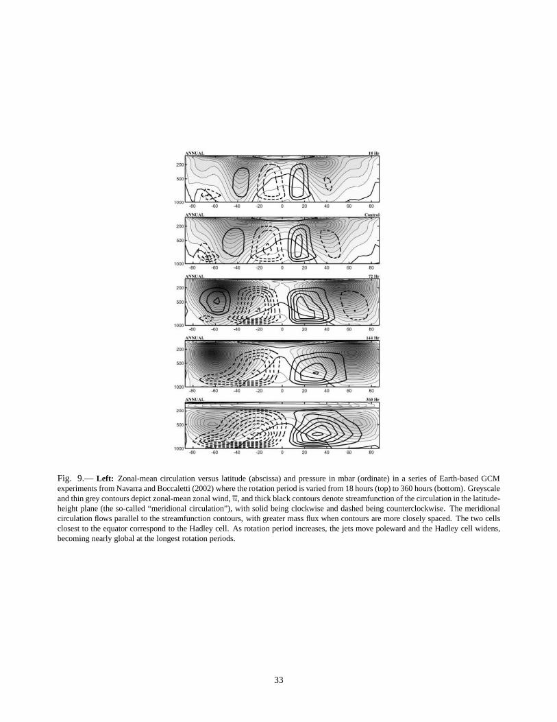
Fig. 9.— Left: Zonal-mean circulation versus latitude (abscissa) and pressure in mbar (ordinate) in a series of Earth-based GCMexperiments from Navarra and Boccaletti (2002) where the rotation period is varied from 18 hours (top) to 360 hours (bottom). Greyscaleand thin grey contours depict zonal-mean zonal wind,u, and thick black contours denote streamfunction of the circulation in the latitude-height plane (the so-called “meridional circulation”), with solid being clockwise and dashed being counterclockwise. The meridionalcirculation flows parallel to the streamfunction contours,with greater mass flux when contours are more closely spaced.The two cellsclosest to the equator correspond to the Hadley cell. As rotation period increases, the jets move poleward and the Hadleycell widens,becoming nearly global at the longest rotation periods.

33

Fig. 10.—Zonally averaged temperature inC versus latitude at 500 mbar (in the mid-troposphere) for a sequence of Earth-like GCMruns that vary the planetary rotation period between 1 and 64Earth days (labelled in the graph). The flat region near the equator ineach run results from the Hadley cell, which transports thermal energy extremely efficiently and leads to a nearly isothermal equatorialtemperature structure. The region of steep temperature gradients at high latitudes is the baroclinic zone, where the temperature structureand latitudinal heat transport are controlled by eddies resulting from baroclinic instability. Note that the width of the Hadley cellincreases, and the equator-to-pole temperature difference decreases, as the planetary rotation period is increased.From del Genio andSuozzo (1987).

At this point, we introduce two constraints. First, Heldand Hou (1980) assumed the circulation is energeticallyclosed, i.e. that no net exchange of mass or thermal energyoccurs between the Hadley cell and higher latitude circula-tions. Given an energy equation with radiation parameter-ized using Newtonian cooling,dθ/dt = (θrad − θ)/τrad,whereτrad is a radiative time constant, the assumption thatthe circulation is steady and closed requires that

∫ φH

0

θ dy =

∫ φH

0

θraddy (64)

where we are integrating from the equator to the polewardedge of the Hadley cell, at latitudeφH . Second, tempera-ture must be continuous with latitude at the poleward edgeof the Hadley cell. In the axisymmetric model, baroclinicinstabilities are suppressed, and the regions poleward of theHadley cells reside in a state of radiative equilibrium. Thus,θ must equalθrad at the poleward edge of the cell. Insert-ing our expressions forθ andθrad into these two constraintsyields a system of two equations forφH andθequator. Thesolution yields a Hadley cell with a latitudinal half-widthof

φH =

(

5∆θradgH

3Ω2a2θ0

)1/2

(65)

in radians. This solution suggests that the width of theHadley cell scales as the square root of the fractionalequator-to-pole radiative-equilibrium temperature differ-ence, the square root of the gravity, the square root ofthe height of the cell, and inversely with the rotationrate. Inserting Earth annual-mean values (∆θrad ≈ 70 K,θ = 260 K, g = 9.8 m sec−2, H = 15 km, a = 6400 km,andΩ = 7.2 × 10−5 sec−1) yields∼ 32.

Redoing this analysis without the small-angle approx-imation leads to a transcendental equation forφH (see

Eq. (17) in Held and Hou 1980), which can be solved nu-merically. Figure 11 (solid curve) illustrates the solution.As expected,φH ranges from0 as Ω → ∞ to 90 asΩ → 0, and, for planets of Earth radius with Hadley cir-culations∼ 10 km tall, bridges these extremes between ro-tation periods of∼ 0.5 and 20 days. Although deviationsexist, the agreement between the simple Held-Hou modeland the 3D GCM is surprisingly good given the simplicityof the Held-Hou model.

Importantly, the Held-Hou model demonstrates that lat-itudinal confinement of the Hadley cell occurs even in anaxisymmetric atmosphere. Thus, the cell’s latitudinal con-finement does not require (for example) three-dimensionalbaroclinic or barotropic instabilities associated with the jetat the poleward branch of the cell. Instead, the confinementresults from energetics: the twin constraints of angular-momentum conservation in the upper branch and thermal-wind balance specify the latitudinal temperature profile inthe Hadley circulation (Eq. 63). This generates equato-rial temperatures colder than (and subtropical temperatureswarmer than) the radiative equilibrium, implying radiativeheating at the equator and cooling in the subtropics. Thisproperly allows the circulation to transport thermal energypoleward. If the cell extended globally on a rapidly ro-tating planet, however, the circulation would additionallyproduce high-latitude temperaturescolder than the radia-tive equilibrium temperature, which in steady state wouldrequire radiativeheatingat high latitudes. This is thermo-dynamically impossible given the specified latitudinal de-pendence ofθrad. The highest latitude to which the cell canextend without encountering this problem is simply givenby Eq. (64).

The model can be generalized to consider a more re-alistic treatment of radiation than the simplified Newto-

34

Fig. 11.— Latitudinal width of the Hadley cell from a sequence of Earth-like GCM runs that vary the planetary rotation period(symbols) and comparison to the Held and Hou (1980) theory (solid curve), the small-angle approximation to the Held-Houtheory fromEq. (65) (dotted curve), and the Held (2000) theory from Eq. (66) (dashed-dotted curve). GCM results are from del Genio and Suozzo(1987) (squares and triangles, depicting northern and southern hemispheres, respectively), Navarra and Boccaletti (2002) (filled circles),and Korty and Schneider (2008) (asterisks; only cases adopting θrad ≈ 70 K and their parameterΓ = 0.7 are shown). Parametersadopted for the curves areg = 9.8 msec

−2, H = 15km, ∆θrad = 70 K, a = 6400 km, θ0 = 260 K, and∆θv = 30K. In the GCMstudies, different authors define the width of the Hadley cell in different ways, so some degree of scatter is inevitable.

nian cooling/heating scheme employed by Held and Hou(1980). Caballero et al. (2008) reworked the scheme using atwo-stream, non-grey representation of the radiative trans-fer with parameters appropriate for Earth and Mars. Thisleads to a prediction for the width of the Hadley cell thatdiffers from Eq. (65) by a numerical constant of order unity.

Although the prediction of Held-Hou-type models forφH provides important insight, several failures of thesemodels exist. First, the model underpredicts the strength ofthe Earth’s Hadley cell (e.g., as characterized by the mag-nitude of the north-south wind) by about an order of mag-nitude. This seems to result from the lack of turbulent ed-dies in axisymmetric models; several studies have shownthat turbulent three-dimensional eddies exert stresses thatact to strengthen the Hadley cells beyond the predictionsof axisymmetric models (e.g. Kim and Lee 2001; Walkerand Schneider 2005, 2006; Schneider 2006).29 Second, theHadley cells on Earth and probably Mars are not energet-ically closed; rather, mid-latitude baroclinic eddies trans-port thermal energy out of the Hadley cell into the polarregions. As a result, net heating occurs throughout the lati-tudinal extent of Earth’s Hadley cell—rather than heating inthe equatorial branch and cooling in the poleward branch aspostulated by Held and Hou (1980). Third, the poleward-moving upper tropospheric branches of the Hadley cells donot conserve angular momentum—although the zonal wind

29Held and Hou (1980)’s original model neglected the seasonalcycle, andit has been suggested that generalization of the Held-Hou axisymmetricmodel to include seasonal effects could alleviate this failing (Lindzen andHou 1988). Although this improves the agreement with Earth’s observedannual-meanHadley-cell strength, it predicts large solstice/equinoxos-cillations in Hadley-cell strength that are lacking in the observed Hadleycirculation (Dima and Wallace 2003).

does become eastward as one moves poleward across thecell, for Earth this increase is a factor of∼ 2–3 less thanpredicted by Eq. (61). Overcoming these failings requiresthe inclusion of three-dimensional eddies.

Several studies have shown that turbulent eddies in themid- to high-latitudes—which are neglected in the Held-Hou and other axisymmetric models—can affect the widthof the Hadley circulation and alter the parameter depen-dences suggested by Eq. (65) (e.g., del Genio and Suozzo1987; Walker and Schneider 2005, 2006). Turbulence canproduce an acceleration/deceleration of the zonal-meanzonal wind, which breaks the angular-momentum conserva-tion constraint in the upper-level wind, causingu to deviatefrom Eq. (61). With a differentu(φ) profile, the latitudi-nal dependence of temperature will change (via Eq. 62),and hence so will the latitudinal extent of the Hadley cellrequired to satisfy Eq. (64). Indeed, within the context ofaxisymmetric models, the addition of strong drag into theupper-layer flow (parameterizing turbulent mixing with theslower-moving surface air, for example) can lead Eq. (64)to predict that the Hadley cell should extend to the poleseven for Earth’s rotation rate (e.g., Farrell 1990).

It could thus be the case that the width of the Hadleycell is strongly controlled by eddies. For example, in themidlatitudes of Earth and Mars, baroclinic eddies generallyaccelerate the zonal flow eastward in the upper troposphere;in steady state, this is generally counteracted by a westwardCoriolis acceleration, which requires anequatorwardup-per tropospheric flow—backwards from the flow directionin the Hadley cell. Such eddy effects can thereby terminatethe Hadley cell, forcing its confinement to low latitudes.Based on this idea, Held (2000) suggested that the Hadley

35

cell width is determined by the latitude beyond which thetroposphere first becomes baroclinically unstable (requir-ing isentrope slopes to exceed a latitude-dependent criticalvalue). Adopting the horizontal thermal gradient impliedby the angular-momentum conserving wind (Eq. 63), mak-ing the small-angle approximation, and utilizing a commontwo-layer model of baroclinic instability, this yields (Held2000)

φH ≈(

gH∆θv

Ω2a2θ0

)1/4

(66)

in radians, where∆θv is the vertical difference in potentialtemperature from the surface to the top of the Hadley cell.Note that the predicted dependence ofφH on planetary ra-dius, gravity, rotation rate, and height of the Hadley cell isweaker than predicted by the Held-Hou model. Earth-basedGCM simulations suggest that Eq. (66) may provide a betterrepresentation of the parameter dependences (Frierson et al.2007; Lu et al. 2007; Korty and Schneider 2008). Neverthe-less, even discrepancies with Eq. (66) are expected since theactual zonal wind does not follow the angular-momentumconserving profile (implying that the actual thermal gradi-ent will deviate from Eq. 63). Substantially more work isneeded to generalize these ideas to the full range of condi-tions relevant for exoplanets.

2.4.4. High-latitude circulations: the baroclinic zones

For terrestrial planets heated at the equator and cooled atthe poles, several studies suggest that the equator-to-poleheat engine can reside in either of two regimes depend-ing on rotation rate and other parameters (del Genio andSuozzo 1987). When the rotation period is long, the Hadleycells extend nearly to the poles, dominate the equator-to-pole heat transport, and thereby determine the equator-to-pole temperature gradient. Baroclinic instabilities are sup-pressed because of the small latitudinal thermal gradientand large Rossby deformation radius (at which baroclinicinstabilities have maximal growth rates), which exceeds theplanetary size for slow rotators such as Titan and Venus.On the other hand, for rapidly rotating planets like Earthand Mars, the Hadley cells are confined to low latitudes;in the absence of eddies the mid- and high-latitudes wouldrelax into a radiative-equilibrium state, leading to minimalequator-to-pole heat transport and a large equator-to-poletemperature difference. This structure is baroclinicallyun-stable, however, and the resulting baroclinic eddies providethe dominant mechanism for transporting thermal energyfrom the poleward edges of the Hadley cells (∼ 30 lati-tude for Earth) to the poles. This baroclinic heat transportsignificantly reduces the equator-to-pole temperature con-trast in the mid- and high-latitudes. For gravity, planetaryradius, and heating rates relevant for Earth, the breakpointbetween these regimes occurs at a rotation period of∼ 5–10days (del Genio and Suozzo 1987).

On rapidly rotating terrestrial planets like Earth andMars, then, the equatorial and high-latitude circulationsfundamentally differ: the equatorial Hadley cells, while

strongly affected by eddies, do notrequire eddies to ex-ist, nor to transport heat poleward. In contrast, the circula-tion and heat transport at high latitudes (poleward of∼ 30

latitude on Earth and Mars) fundamentally depends on theexistence of eddies. At high latitudes, interactions of ed-dies with the mean flow controls the latitudinal tempera-ture gradient, latitudinal heat transport, and structure of thejet streams. This range of latitudes is called thebarocliniczone.

The extent to which baroclinic eddies can reduce theequator-to-pole temperature gradient has important impli-cations for the mean climate. Everything else being equal,an Earth-like planet with colder poles will develop more ex-tensive polar ice and be more susceptible to an ice-albedofeedback that triggers a globally glaciated “snowball” state(Spiegel et al. 2008). Likewise, a predominantly CO2 at-mosphere can become susceptible to atmospheric collapseif the polar temperatures become sufficiently cold for CO2

condensation.There is thus a desire to understand the extent to which

baroclinic eddies can transport heat poleward. General cir-culation models (GCMs) attack this problem by spatiallyand temporally resolving the full life of every barocliniceddy and their effect on the mean state, but this is com-putationally intensive and often sheds little light on the un-derlying sensitivity of the process to rotation rate and otherparameters.

Two simplified approaches have been advanced that illu-minate this issue. Although GCMs for terrestrial exoplanetswill surely be needed in the future, simplified approachescan guide our understanding of such GCM results and pro-vide testable hypotheses regarding the dependence of heattransport on planetary parameters. They also may provideguidance for parameterizations of the latitudinal heat trans-port in simpler energy-balance climate models that do notexplicitly attempt to resolve the full dynamics. We devotethe rest of this section to discussing these simplified ap-proaches.

The first simplified approach postulates that barocliniceddies relax the midlatitude thermal structure into a statethat is neutrally stable to baroclinic instabilities (Stone1978), a process calledbaroclinic adjustment. This ideais analogous to the concept of convective adjustment: whenradiation or other processes drive the vertical temperaturegradient steeper than an adiabat (dT/dz < −g/cp foran ideal gas, wherez is height), convection ensues anddrives the temperature profile toward the adiabat, whichis the neutrally stable state for convection. If the convec-tive overturn timescales are much shorter than the radiativetimescales, then convection overwhelms the ability of ra-diation to destabilize the environment, and the temperatureprofile then deviates only slightly from an adiabat over awide range of convective heat fluxes (see, e.g.,§2.3.1). Ina similar way, the concept of baroclinic adjustment postu-lates that when timescales for baroclinic eddy growth aremuch shorter than the timescale for radiation to create alarge equator-to-pole temperature contrast, the eddies will

36

transport thermal energy poleward at just the rate needed tomaintain a profile that is neutral to baroclinic instabilities.

This idea was originally developed for a simplified two-layer system, for which baroclinic instability first initiateswhen the slope of isentropes exceeds∼ H/a, whereH isa pressure scale height anda is the planetary radius. Com-parison of this critical isentrope slope with Earth observa-tions shows impressive agreement poleward of 30-40 lati-tude, where baroclinic instabilities are expected to be active(Stone 1978). A substantial literature has subsequently de-veloped to explore the idea further (for a review see Zurita-Gotor and Lindzen 2006). The resulting latitudinal temper-ature gradient is then approximatelyH/a times the verti-cal potential temperature gradient. Interestingly, this the-ory suggests that otherwise identical planets with differentBrunt-Vaisala frequencies (due to differing opacitiesand/orroles for latent heating, for example) would exhibit very dif-ferent midlatitude temperature gradients—the planet withsmaller stable stratification (i.e., smaller Brunt-Vais¨ala fre-quency; Eq. 6) exhibiting a smaller latitudinal temperaturegradient. Moreover, although Earth’s ocean transports sub-stantial heat between the equator and poles, the theory alsosuggests that the ocean may only exert a modest influenceon the latitudinal temperature gradients in theatmosphere(Lindzen and Farrell 1980a): in the absence of oceanicheat transport, the atmospheric eddies would simply take upthe slack to maintain the atmosphere in the baroclinicallyneutral state. (There could of course be an indirect effecton latitudinal temperature gradients if removing/adding theoceans altered the tropospheric stratification.) Finally,thetheory suggests that the latitudinal temperature gradientinthe baroclinic zone does not depend on planetary rotationrate except indirectly via the influence of rotation rate onstatic stability. It is worth emphasizing, however, that evenif the latitudinal temperature gradientin the baroclinic zonewere constant with rotation rate, the total equator-to-poletemperature difference would still decrease with decreas-ing rotation rate because, with decreasing rotation rate, theHadley cell occupies a greater latitude range and the baro-clinically adjusted region would be compressed toward thepoles (see Fig.10).

Despite Stone (1978)’s encouraging results, severalcomplicating factors exist. First, the time-scale separa-tion between radiation and dynamics is much less obvi-ous for baroclinic adjustment than for convective adjust-ment. In an Earth or Mars-like context, the convectiveinstability timescales are∼ 1 hour, the baroclinic insta-bility timescales are days, and the radiation timescale is∼ 20 days (Earth) or∼ 2 days (Mars). The ability of baro-clinic eddies to adjust the environment to a baroclinicallyneutral state may thus be marginal, especially for planetswith short radiative time constants (such as Mars). Sec-ond, the neutrally stable state in the two-layer model—corresponding to an isentrope slope of∼ H/a—is an arte-fact of the vertical discretization in that model. When amulti-layer model is used, the critical isentrope slope forinitiating baroclinic instability decreases as the numberof

layers increases, and it approaches zero in a vertically con-tinuous model. One might then wonder why a barocliniczone can supportany latitudinal temperature contrast (as itobviously does on Earth and Mars). The reason is that theinstability growth timescales are long at small isentropicslopes (Lindzen and Farrell 1980b); the instabilities onlydevelop a substantial ability to affect the mean state whenisentrope slopes become steep. In practice, then, the baro-clinic eddies are perhaps only able to relax the atmosphereto a state with isentrope slopes of∼ H/a rather than some-thing significantly shallower.

The second simplified approach to understanding equator-to-pole temperature contrasts on terrestrial planets seeks todescribe the poleward heat transport by baroclinic eddies asa diffusive process (Held 1999). This approach is based onthe idea that baroclinic eddies have maximal growth rates atscales close to the Rossby radius of deformation,LD (seeEq. 32), and if the baroclinically unstable zone has a latitu-dinal width substantially exceedingLD then there will bescale separation between the mean flow and the eddies.30

The possible existence of a scale separation in the baro-clinic instability problem implies that representing the heattransport as a function oflocal mean-flow quantities (suchas the mean latitudinal temperature gradient) is a reason-able prospect. Still, caution is warranted, since an inverseenergy cascade (§2.2.6) could potentially transfer the en-ergy to scales larger thanLD, thereby weakening the scaleseparation.

The diffusive approach is typically cast in the contextof a 1D energy-balance model that seeks to determine thevariation with latitude of the zonally averaged surface tem-perature. This approach has a long history for Earth climatestudies (see review in North et al. 1981), solar-system plan-ets (e.g. Hoffert et al. 1981), and even in preliminary stud-ies of the climates and habitability of extrasolar terrestrialplanets (Williams and Kasting 1997; Williams and Pollard2003; Spiegel et al. 2008, 2009). In its simplest form, thegoverning equation reads

c∂T

∂t= ∇ · (cD∇T ) + S(φ) − I (67)

whereT is surface temperature,D ( m2 sec−1) is the dif-fusivity associated with heat transport by baroclinic eddies,S(φ) is the absorbed stellar flux as a function of latitude,andI is the emitted thermal flux, which is a function of tem-perature. In the simplest possible case,I is represented asa linear function of temperature,I = A+BT (North et al.1981), whereA andB are positive constants. In Eq. (67),cis a heat capacity (with unitsJ m−2 K−1) that represents theatmosphere and oceans (if any). The steady-state solutionin the absence of transport (D = 0) is T = [S(φ) −A]/B.

30As pointed out by Held (1999), this differs from many instability problemsin fluid mechanics, such as shear instability in pipe flow or convection in afluid driven by a heat flux between two plates, where maximal growth ratesoccur at length scales comparable to the domain size and no eddy/mean-flow scale separation occurs.

37

On the other hand, when transport dominates (D → ∞),the solution yields constantT .

The termS(φ) includes the effect of latitudinally varyingalbedo (e.g., due to ice cover), but if albedo is constant withlatitude, thenS represents the latitudinally varying insola-tion. To schematically illustrate the effect of heat transporton the equator-to-pole temperature gradient, parameterizeSas a constant plus a term proportional to the Legendre poly-nomialP2(cosφ). In this case, and ifD andc are constant,the equation has a steady analytic solution with an equator-to-pole temperature difference given by (Held 1999)

∆Teq−pole =∆Trad

1 + 6 cDBa2

(68)

wherea is the planetary radius and∆Trad is the equator-to-pole difference in radiative-equilibrium temperature. Theequation implies that atmospheric heat transport signifi-cantly influences the equator-to-pole temperature differencewhen the diffusivity exceeds∼ Ba2/(6c). For Earth,B ≈2 W m−2 K−1, a = 6400 km, and c ≈ 107 J m−2 K−1,suggesting that atmospheric transport becomes importantwhenD & 106 m2 sec−1.

The question comes down to how to determine the diffu-sivity,D. In Earth models,D is typically chosen by tuningthe models to match the current climate, and then that valueof D is used to explore the regimes of other climates (e.g.North 1975). However, that approach sidesteps the underly-ing physics and prevents an extrapolation to other planetaryenvironments.

Motivated by an interest in understanding the feedbackbetween baroclinic instabilities and the mean state, substan-tial effort has been devoted to determining the dependenceof the diffusivity on control parameters such as rotationrate and latitudinal thermal gradient (for a review see Held1999). This work can help guide efforts to understand thetemperature distribution on rapidly rotating exoplanets.Weexpect that the diffusivity will scale as

D ≈ ueddyLeddy (69)

where ueddy and Leddy are the characteristic velocitiesand horizontal sizes of the heat-transporting eddies. Be-cause baroclinic eddies will be in near-geostrophic balance(Eq. 30) on a rapidly rotating planet, the characteristic eddyvelocities,ueddy, will relate to characteristic eddy potential-temperature perturbationsθ′eddy via the thermal-wind rela-tion, givingueddy ∼ gθ′eddyheddy/(fLeddy), whereheddy

is the characteristic vertical thickness of the eddies. Underthe assumption that the ratio of vertical to horizontal scalesis heddy/Leddy ∼ f/N (Charney 1971; Haynes 2005), thisyieldsueddy ≈ gθ′eddy/(θ0N) (whereN is Brunt-Vaisalafrequency), which simply states that eddies with larger ther-mal perturbations will also have larger velocity perturba-tions. Under the assumption that the thermal perturbationsscale asθ′eddy ≈ Leddy∂θ/∂y, we then have

D ≈ L2eddy

g

Nθ0

∂θ

∂y. (70)

Greater thermal gradients and eddy-length scales lead togreater diffusivity and, importantly, the diffusivity dependson thesquareof the eddy size.

Several proposals for the relevant eddy size have beenput forward, which we summarize in Table 2. Based onthe idea that baroclinic instabilities have the greatest growthrates for lengths comparable to the deformation radius,Stone (1972) suggested thatLeddy is the deformation ra-dius,NH/f . On the other hand, baroclinic eddies couldenergize an inverse cascade, potentially causing the domi-nant heat-transporting eddies to have sizes exceedingLD.In the limit of this process (Green 1970), the eddies wouldreach the width of the baroclinic zone,Lzone (potentiallyclose to a planetary radius for a planet with a narrow Hadleycell). This simply leads to Eq. (70) withLeddy = Lzone. Incontrast, Held and Larichev (1996) argued that the inversecascade would produce an eddy scale not of orderLzone butinstead of order the Rhines scale,(ueddy/β)1/2. Finally,Barry et al. (2002) used heat-engine arguments to proposethat

D ≈(

eaq

θ0

∂θ

∂y

)3/5 (

2

β

)4/5

(71)

whereqnet is the net radiative heating/cooling per mass thatthe eddy fluxes are balancing,a is the planetary radius, ande is a constant of order unity.

As can be seen in Table 2, these proposals have diver-gent implications for the dependence of diffusivity on back-ground parameters. Stone (1972)’s diffusivity is propor-tional to the latitudinal temperature gradient and, becauseof the variation ofLD with rotation rate, inversely propor-tional to the square of the planetary rotation rate. Green(1970)’s diffusivity likewise scales with the latitudinaltem-perature gradient; it contains no explicit dependence on theplanetary rotation rate, but a rotation-rate dependence couldenter because the Hadley cell shrinks andLzone increaseswith increasing rotation rate. Held and Larichev (1996)’sdiffusivity has the same rotation-rate dependence as that ofStone (1972), but it has a much stronger depenence on grav-ity and temperature gradient [g3 and(∂θ/∂y)3]. Moreover,it increases with decreasing static stability asN−3, un-like Stone’s diffusivity that scales withN .31 Finally, Barryet al. (2002)’s diffusivity suggests a somewhat weaker de-pendence, scaling with as(∂θ/∂y)3/5 and Ω−3/5. Notethat the rotation-rate dependences described above shouldbe treated with caution, because altering the rotation rateorgravity could change the circulation in a way that alters theBrunt-Vaisala frequency, leading to additional changes in

31TheN−3 dependence in Held and Larichev (1996)’s gives the impres-sion that the diffusivity becomes unbounded as the atmospheric verti-cal temperature profile becomes neutrally stable (i.e. asN → 0), butthis is misleading. In reality, one expects the latitudinaltemperaturegradient and potential energy available for driving baroclinic instabili-ties to decrease with decreasingN . Noting that the slope of isentropesis mθ ≡ (∂θ/∂y)(∂θ/∂z)−1 , one can re-express Held and Larichev(1996)’s diffusivity as scaling withmθN

3. Thus, at constant isentropeslope, the diffusivity properly drops to zero as the vertical temperatureprofile becomes neutrally stable.

38

TABLE 2

PROPOSED DIFFUSIVITIES FOR HIGH-LATITUDE HEAT TRANSPORT ON TERRESTIAL PLANETS

Scheme Leddy D

Stone (1972) LDH2Ngf2θ0

∂θ∂y

Green (1970) Lzone L2zone

gNθ0

∂θ∂y

Held and Larichev (1996) Lβg3

N3β2θ3

0

“

∂θ∂y

”3

Barry et al. (2002) Lβ

“

eaqnet

θ0

∂θ∂y

”3/5 “

2β

”4/5

the diffusivity.Additional work is needed to determine which of these

schemes (if any) is valid over a wide range of parametersrelevant to terrestrial exoplanets. Most of the work per-formed to test the schemes of Green (1970), Stone (1972),Held and Larichev (1996) and others has adopted simpli-fied two-layer quasi-geostrophic models under idealized as-sumptions such as planar geometry with constant Coriolisparameter (a so-called “f-plane”). Because variation offwith latitude alters the properties of baroclinic instability, itis possible that schemes developed for constantf may nottranslate directly into a planetary context. In contrast, Barryet al. (2002) performed a suite of Earth-based full GCM cal-culations (which had 33 layers and properly account for thevariation off across the sphere) to test the various diffusiv-ities proposed above, and they found that Eq. (71) providesthe best fit to the GCM results. Their results are proba-bly most robust for the dependences on heating rateqnet

and thermal gradient∂θ/∂y, which they varied by factorsof ∼ 200 and 6, respectively; planetary radius and rotationrates were varied by only∼ 70%, so the dependences onthose parameters should be considered tentative. Additionalsimulations in the spirit of Barry et al. (2002), consideringa wider range of planetary and atmospheric parameters, canclarify the true sensitivities of the heat transport rates.

2.4.5. Slowly rotating regime

At slow rotation rates, the GCM simulations shown inFigs. 9–10 develop near-global Hadley cells with high-latitude jets, but the wind remains weak at the equator. Incontrast, Titan and Venus (with rotation periods of 16 and243 days, respectively) have robust (∼100 m sec−1) super-rotating winds in their equatorial upper tropospheres. Be-cause the equator is the region of the planet lying farthestfrom the rotation axis, such a flow contains a local maxi-mum of angular momentum at the equator. AxisymmetricHadley circulations (§2.4.3) cannot produce such superro-tation; rather, up-gradient transport of momentum by ed-dies is required. This process remains poorly understood.One class of models suggests that this transport occurs from

high latitudes; for example, the high-latitude jets that resultfrom the Hadley circulation (which can be seen in Fig. 9)experience a large-scale shear instability that pumps eddymomentum toward the equator, generating the equatorialsuperrotation (Del Genio and Zhou 1996). Alternatively,thermal tide or wave interaction could induce momentumtransports that generate the equatorial superrotation (e.g.,Fels and Lindzen 1974). Recently, a variety of simplifiedVenus and Titan GCMs have been developed that show en-couraging progress in capturing the superrotation (e.g., Ya-mamoto and Takahashi 2006; Richardson et al. 2007; Leeet al. 2007; Herrnstein and Dowling 2007).

The Venus/Titan superrotation problem may have impor-tant implications for understanding the circulation of syn-chronously locked exoplanets. All published 3D circulationmodels of synchronously locked hot Jupiters (§2.3.3), andeven the few published studies of sychrounously locked ter-restrial planets (Joshi et al. 1997; Joshi 2003, see§2.4.6),develop robust equatorial superrotation. The day-nightheating pattern associated with synchronous locking shouldgenerate thermal tides and, in analogy with Venus and Ti-tan, these could be relevant in driving the superrotationin the 3D exoplanet models. Simplified Earth-based two-layer calculations that include longitudinally varying heat-ing, and which also develop equatorial superrotation, seemto support this possibility (Suarez and Duffy 1992; Sara-vanan 1993).

2.4.6. Unusual forcing regimes

Our discussion of circulation regimes on terrestrial plan-ets has so far largely focused on annual-mean forcing con-ditions. On Earth, seasonal variations represent relativelymodest perturbations around the annual-mean climate dueto Earth’s23.5 obliquity. On longer timescales, the secu-lar evolution of Earth’s orbital elements is thought to be re-sponsible for paleoclimatic trends, such as ice ages, accord-ing to Milankovitch’s interpretation (e.g. Kawamura et al.2007). While it may be surprising to refer to Earth’s seasonsor ice ages as minor events from a human perspective, it isclear that they constitute rather mild versions of the more

39

diverse astronomical forcing regimes expected to occur onextrasolar worlds.

In principle, terrestrial exoplanets could possess largeobliquities (i → 90 deg) and eccentricities (e → 1). Thiswould result in forcing conditions with substantial seasonalvariations around the annual mean, such as order-of magni-tude variations in the global insolation over the orbital pe-riod at large eccentricities. Even the annual mean climatecan be dramatically affected under unusual forcing condi-tions, for instance at large obliquities when the poles receivemore annual-mean insolation than the planetary equator (fori > 54). Yet another unusual forcing regime occurs if theterrestrial planet is tidally locked to its parent star and thuspossesses permanent day and night sides much like the hotJupiters discussed in§2.3.3. Relatively few studies of circu-lation regimes under such unusual forcing conditions havebeen carried out to date.

Williams and Kasting (1997) and Spiegel et al. (2009)investigated the climate of oblique Earth-like planets withsimple, diffusive energy-balance models of the type de-scribed by Eq. (67). While seasonal variations were foundto be severe at high obliquity, Williams and Kasting (1997)concluded that highly oblique planets could neverthelessremain regionally habitable, especially if they possessedthick CO2-enriched atmospheres with large thermal iner-tia relative to Earth, as may indeed be expected for terres-trial planets in the outermost regions of a system’s habit-able zone. Spiegel et al. (2009) confirmed these results andhighlighted the risks that global glaciation events and partialatmospheric CO2 collapse constitute for highly oblique ter-restrial exoplanets. Williams and Pollard (2003) presenteda much more detailed set of three-dimensional climate andcirculation models for Earth-like planets at various obliq-uities. Despite large seasonal variations at extreme obliq-uities, Williams and Pollard (2003) found no evidence forany runaway greenhouse effect or global glaciation eventin their climate models and thus concluded that Earth-likeplanets should generally be hospitable to life even at highobliquity.

Williams and Pollard (2002) also studied the climateon eccentric versions of the Earth with a combinationof detailed three-dimensional climate models and simplerenergy-balance models. They showed that the strong vari-ations in insolation occurring at large eccentricities canberather efficiently buffered by the large thermal inertia ofthe atmosphere+ocean climate system. These authors thusargued that the annually averaged insolation, which is anincreasing function ofe, may be the most meaningful quan-tity to describe in simple terms the climate of eccentric,thermally blanketed Earth-like planets. It is presumablythe case that terrestrial planets with reduced thermal iner-tia from lower atmospheric/oceanic masses would be morestrongly affected by such variations in insolation.

It should be emphasized that, despite the existing workon oblique or eccentric versions of the Earth, a fundamen-tal understanding of circulation regimes under such unusualforcing conditions is still largely missing. For instance,

variations in the Hadley circulation regime or the baro-clinic transport efficiency, expected as forcing conditionsvary along the orbit, have not been thoroughly explored.Similarly, the combined effects of a substantial obliquityand eccentricity have been ignored. As the prospects forfinding and characterizing exotic versions of the Earth im-prove, these issues should become the subject of increasingscrutiny.

One of the best observational prospects for the nextdecade is the discovery of tidally locked terrestrial plan-ets around nearby M-dwarfs (e.g., Irwin et al. 2009; Sea-ger et al. 2008). In anticipation of such discoveries, Joshiet al. (1997) presented a careful investigation of the circu-lation regime on this class of unusually forced planets, withpermanent day and night sides. The specific focus of theirwork was to determine the conditions under which CO2 at-mospheric collapse could occur on the cold night sides ofsuch planets and act as a trap for this important greenhousegas, even when circulation and heat transport are present.Using a simplified general circulation model, these authorsexplored the problem’s parameter space for various globalplanetary and atmospheric attributes and included a studyof the potential risks posed by violent flares from the stel-lar host. The unusual circulation regime that emerged fromthis work was composed of a direct circulation cell at sur-face levels (i.e. equatorial day to night transport with po-lar return) and a superrotating wind higher up in the atmo-sphere. While detrimental atmospheric collapse did occurunder some combinations of planetary attributes (e.g., forthin atmospheres), the authors concluded that efficient at-mospheric heat transport was sufficient to prevent collapseunder a variety of plausible scenarios. More recently, Joshi(2003) revisited some of these results with a much moredetailed climate model with explicit treatments of non-grayradiative transfer and a hydrological cycle. It is likely thatthis interesting circulation regime will be reconsidered inthe next few years as the discovery of such exotic worlds ison our horizon.

3. FUTURE PROSPECTS

Over the past few years, transit, secondary eclipse, andlight curve observations have provided our first look atthe atmospheric structure and circulation of several hotJupiters. The reality of atmospheric circulation on these ob-jects is suggested by exquisite light curves of HD 189733bshowing modest day-night infrared brightness tempera-ture variations and displacement of the longitudes of min-imum/maximum flux from the antistellar/substellar points,presumably the result of an efficient circulation able to dis-tort the temperature pattern (Knutson et al. 2007, 2009).However, observations of a range of hot Jupiters and Nep-tunes hint at a diversity of behaviors that has yet to befully characterized. In parallel, this observational vanguardhas triggered a growing body of theoretical and modelingstudies to investigate plausible atmospheric circulationpat-terns on hot Jupiters. While the models agree on some

40

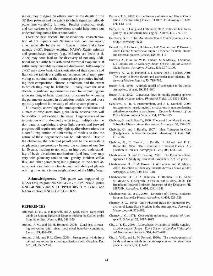
issues, they disagree on others, such as the details of the3D flow patterns and the extent to which significant global-scale time variability is likely. Further theoretical workand comparison with observations should help move ourunderstanding onto a firmer foundation.

Over the next decade, the observational characteriza-tion of hot Jupiters and Neptunes will continue apace,aided especially by the warmSpitzermission and subse-quently JWST. Equally exciting, NASA’sKepler missionand groundbased surveys (e.g., MEarth; see Irwin et al.2009) may soon lead to the discovery of not only addi-tional super-Earths but Earth-sized terrestrial exoplanets. Ifsufficiently favorable systems are discovered, follow-up byJWSTmay allow basic characterization of their spectra andlight curves (albeit at significant resources per planet), pro-viding constraints on their atmospheric properties includ-ing their composition, climate, circulation, and the extentto which they may be habitable. Finally, over the nextdecade, significant opportunities exist for expanding ourunderstanding of basic dynamical processes by wideningthe parameters adopted in circulation models beyond thosetypically explored in the study of solar-system planets.

Ultimately, unraveling the atmospheric circulation andclimate of exoplanets from global-scale observations willbe a difficult yet exciting challenge. Degeneracies of in-terpretation will undoubtedly exist (e.g., multiple circula-tion patterns explaining a given light curve), and forwardprogress will require not only high-quality observations buta careful exploration of a hierarchy of models so that thenature of these degeneracies can be understood. Despitethe challenge, the potential payoff will be the unleashingof planetary meteorology beyond the confines of our So-lar System, leading to not only an improved understand-ing of basic circulation mechanisms (and how they mayvary with planetary rotation rate, gravity, incident stellarflux, and other parameters) but a glimpse of the actual at-mospheric circulations, climate, and habitability of planetsorbiting other stars in our neighborhood of the Milky Way.

Acknowledgments. This paper was supported byNASA Origins grant NNX08AF27G to APS, NASA grantsNNG04GN82G and STFC PP/E001858/1 to JYKC, andNASA contract NNG06GF55G to KM.

REFERENCES

Atkinson, D. H., A. P. Ingersoll, and A. Seiff, 1997: Deep zonalwinds on Jupiter: Update of Doppler tracking the Galileo probefrom the orbiter.Nature, 388, 649–650.

Aurnou, J. M., and M. H. Heimpel, 2004: Zonal jets in rotat-ing convection with mixed mechanical boundary conditions.Icarus, 169, 492–498.

Aurnou, J. M., and P. L. Olson, 2001: Strong zonal winds fromthermal convection in a rotating spherical shell.Geophys. Res.Lett., 28, 2557–2560.

Barman, T. S., 2008: On the Presence of Water and Global Circu-lation in the Transiting Planet HD 189733b.Astrophys. J. Lett.,676, L61–L64.

Barry, L., G. C. Craig, and J. Thuburn, 2002: Poleward heat trans-port by the atmospheric heat engine.Nature, 415, 774–777.

Batchelor, G. K., 1967:An Introduction to Fluid Dynamics. Cam-bridge University Press.

Bezard, B., E. Lellouch, D. Strobel, J.-P. Maillard, and P.Drossart,2002: Carbon Monoxide on Jupiter: Evidence for Both Internaland External Sources.Icarus, 159, 95–111.

Burrows, A., T. Guillot, W. B. Hubbard, M. S. Marley, D. Saumon,J. I. Lunine, and D. Sudarsky, 2000: On the Radii of Close-inGiant Planets.Astrophys. J. Lett., 534, L97–L100.

Burrows, A., W. B. Hubbard, J. I. Lunine, and J. Liebert, 2001:The theory of brown dwarfs and extrasolar giant planets.Re-views of Modern Physics, 73, 719–765.

Busse, F. H., 1976: A simple model of convection in the Jovianatmosphere.Icarus, 29, 255–260.

Busse, F. H., 2002: Convective flows in rapidly rotating spheresand their dynamo action.Physics of Fluids, 14, 1301–1314.

Caballero, R., R. T. Pierrehumbert, and J. L. Mitchell, 2008:Axisymmetric, nearly inviscid circulations in non-condensingradiative-convective atmospheres.Quarterly Journal of theRoyal Meteorological Society, 134, 1269–1285.

Chabrier, G., and I. Baraffe, 2000: Theory of Low-Mass StarsandSubstellar Objects.Annu. Rev. Astron. Astrophys., 38, 337–377.

Chabrier, G., and I. Baraffe, 2007: Heat Transport in Giant(Exo)planets: A New Perspective.Astrophys. J. Lett., 661,L81–L84.

Chabrier, G., T. Barman, I. Baraffe, F. Allard, and P. H.Hauschildt, 2004: The Evolution of Irradiated Planets: Ap-plication to Transits.Astrophys. J. Lett., 603, L53–L56.

Charbonneau, D., and D. Deming, 2007: The Dynamics-BasedApproach to Studying Terrestrial Exoplanets.ArXiv e-prints.

Charbonneau, D., T. M. Brown, D. W. Latham, and M. Mayor,2000: Detection of Planetary Transits Across a Sun-like Star.Astrophys. J. Lett., 529, L45–L48.

Charbonneau, D., H. A. Knutson, T. Barman, L. E. Allen,M. Mayor, S. T. Megeath, D. Queloz, and S. Udry, 2008: TheBroadband Infrared Emission Spectrum of the Exoplanet HD189733b.Astrophys. J., 686, 1341–1348.

Charbonneau, D., et al., 2005: Detection of Thermal Emissionfrom an Extrasolar Planet.Astrophys. J., 626, 523–529.

Charney, J. G., 1949: On a Physical Basis for Numerical Pre-diction of Large-Scale Motions in the Atmosphere.Journal ofMeteorology, 6, 371–385.

Charney, J. G., 1971: Geostrophic turbulence.Journal of Atmo-spheric Sciences, 28, 1087–1095.

Cho, J. Y.-K., 2008: Atmospheric dynamics of tidally synchro-nized extrasolar planets.Royal Society of London Philosophi-cal Transactions Series A, 366, 4477–4488.

Cho, J. Y.-K., and L. M. Polvani, 1996a: The morphogenesis ofbands and zonal winds in the atmospheres on the giant outerplanets.Science, 8(1), 1–12.

41

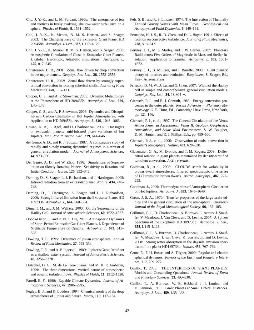
Cho, J. Y.-K., and L. M. Polvani, 1996b: The emergence of jetsand vortices in freely evolving, shallow-water turbulenceon asphere.Physics of Fluids, 8, 1531–1552.

Cho, J. Y.-K., K. Menou, B. M. S. Hansen, and S. Seager,2003: The Changing Face of the Extrasolar Giant Planet HD209458b.Astrophys. J. Lett., 587, L117–L120.

Cho, J. Y.-K., K. Menou, B. M. S. Hansen, and S. Seager, 2008:Atmospheric Circulation of Close-in Extrasolar Giant Planets.I. Global, Barotropic, Adiabatic Simulations.Astrophys. J.,675, 817–845.

Christensen, U. R., 2001: Zonal flow driven by deep convectionin the major planets.Geophys. Res. Lett., 28, 2553–2556.

Christensen, U. R., 2002: Zonal flow driven by strongly super-critical convection in rotating spherical shells.Journal of FluidMechanics, 470, 115–133.

Cooper, C. S., and A. P. Showman, 2005: Dynamic Meteorologyat the Photosphere of HD 209458b.Astrophys. J. Lett., 629,L45–L48.

Cooper, C. S., and A. P. Showman, 2006: Dynamics and Disequi-librium Carbon Chemistry in Hot Jupiter Atmospheres, withApplication to HD 209458b.Astrophys. J., 649, 1048–1063.

Cowan, N. B., E. Agol, and D. Charbonneau, 2007: Hot nightson extrasolar planets: mid-infrared phase variations of hotJupiters.Mon. Not. R. Astron. Soc., 379, 641–646.

del Genio, A. D., and R. J. Suozzo, 1987: A comparative study ofrapidly and slowly rotating dynamical regimes in a terrestrialgeneral circulation model.Journal of Atmospheric Sciences,44, 973–986.

Del Genio, A. D., and W. Zhou, 1996: Simulations of Superro-tation on Slowly Rotating Planets: Sensitivity to RotationandInitial Condition. Icarus, 120, 332–343.

Deming, D., S. Seager, L. J. Richardson, and J. Harrington, 2005:Infrared radiation from an extrasolar planet.Nature, 434, 740–743.

Deming, D., J. Harrington, S. Seager, and L. J. Richardson,2006: Strong Infrared Emission from the Extrasolar Planet HD189733b.Astrophys. J., 644, 560–564.

Dima, I. M., and J. M. Wallace, 2003: On the Seasonality of theHadley Cell.Journal of Atmospheric Sciences, 60, 1522–1527.

Dobbs-Dixon, I., and D. N. C. Lin, 2008: Atmospheric Dynamicsof Short-Period Extrasolar Gas Giant Planets. I. Dependence ofNightside Temperature on Opacity.Astrophys. J., 673, 513–525.

Dowling, T. E., 1995: Dynamics of jovian atmospheres.AnnualReview of Fluid Mechanics, 27, 293–334.

Dowling, T. E., and A. P. Ingersoll, 1989: Jupiter’s Great Red Spotas a shallow water system.Journal of Atmospheric Sciences,46, 3256–3278.

Dritschel, D. G., M. de La Torre Juarez, and M. H. P. Ambaum,1999: The three-dimensional vortical nature of atmosphericand oceanic turbulent flows.Physics of Fluids, 11, 1512–1520.

Farrell, B. F., 1990: Equable Climate Dynamics.Journal of At-mospheric Sciences, 47, 2986–2995.

Fegley, B. J., and K. Lodders, 1994: Chemical models of the deepatmospheres of Jupiter and Saturn.Icarus, 110, 117–154.

Fels, S. B., and R. S. Lindzen, 1974: The Interaction of ThermallyExcited Gravity Waves with Mean Flows.Geophysical andAstrophysical Fluid Dynamics, 6, 149–191.

Fernando, H. J. S., R.-R. Chen, and D. L. Boyer, 1991: Effectsofrotation on convective turbulence.Journal of Fluid Mechanics,228, 513–547.

Fortney, J. J., M. S. Marley, and J. W. Barnes, 2007: PlanetaryRadii across Five Orders of Magnitude in Mass and Stellar In-solation: Application to Transits.Astrophys. J., 659, 1661–1672.

Fortney, J. J., B. Militzer, and I. Baraffe, 2009: Giant planets:theory of interiors and evolution.Exoplanets, S. Seager, Ed.,Univ. Arizona Press.

Frierson, D. M. W., J. Lu, and G. Chen, 2007: Width of the Hadleycell in simple and comprehensive general circulation models.Geophys. Res. Lett., 34, 18,804–+.

Gierasch, P. J., and B. J. Conrath, 1985: Energy conversion pro-cesses in the outer planets.Recent Advances in Planetary Me-teorology, G. E. Hunt, Ed., Cambridge Univ. Press, New York,pp. 121–146.

Gierasch, P. J., et al., 1997: The General Circulation of theVenusAtmosphere: an Assessment.Venus II: Geology, Geophysics,Atmosphere, and Solar Wind Environment, S. W. Bougher,D. M. Hunten, and R. J. Philips, Eds., pp. 459–500.

Gierasch, P. J., et al., 2000: Observation of moist convection inJupiter’s atmosphere.Nature, 403, 628–630.

Glatzmaier, G. A., M. Evonuk, and T. M. Rogers, 2009: Differ-ential rotation in giant planets maintained by density-stratifiedturbulent convection.ArXiv e-prints.

Goldman, B., et al., 2008: CLOUDS search for variability inbrown dwarf atmospheres. Infrared spectroscopic time seriesof L/T transition brown dwarfs.Astron. Astrophys., 487, 277–292.

Goodman, J., 2009: Thermodynamics of Atmospheric Circulationon Hot Jupiters.Astrophys. J., 693, 1645–1649.

Green, J. S. A., 1970: Transfer properties of the large-scale ed-dies and the general circulation of the atmosphere.QuarterlyJournal of the Royal Meteorological Society, 96, 157–185.

Grillmair, C. J., D. Charbonneau, A. Burrows, L. Armus, J. Stauf-fer, V. Meadows, J. Van Cleve, and D. Levine, 2007: A SpitzerSpectrum of the Exoplanet HD 189733b.Astrophys. J. Lett.,658, L115–L118.

Grillmair, C. J., A. Burrows, D. Charbonneau, L. Armus, J. Stauf-fer, V. Meadows, J. van Cleve, K. von Braun, and D. Levine,2008: Strong water absorption in the dayside emission spec-trum of the planet HD189733b.Nature, 456, 767–769.

Grote, E., F. H. Busse, and A. Tilgner, 2000: Regular and chaoticspherical dynamos.Physics of the Earth and Planetary Interi-ors, 117, 259–272.

Guillot, T., 2005: THE INTERIORS OF GIANT PLANETS:Models and Outstanding Questions.Annual Review of Earthand Planetary Sciences, 33, 493–530.

Guillot, T., A. Burrows, W. B. Hubbard, J. I. Lunine, andD. Saumon, 1996: Giant Planets at Small Orbital Distances.Astrophys. J. Lett., 459, L35–L38.

42

Guillot, T., D. J. Stevenson, W. B. Hubbard, and D. Saumon, 2004:The interior of Jupiter.Jupiter: The Planet, Satellites and Mag-netosphere, F. Bagenal, T. E. Dowling, and W. B. McKinnon,Eds., Cambridge Univ. Press, pp. 35–57.

Harrington, J., B. M. Hansen, S. H. Luszcz, S. Seager, D. Deming,K. Menou, J. Y.-K. Cho, and L. J. Richardson, 2006: ThePhase-Dependent Infrared Brightness of the Extrasolar Planetυ Andromedae b.Science, 314, 623–626.

Hartmann, D. L., and coauthors, 2003:Understanding ClimateChange Feedbacks. National Research Council of the NationalAcademy of Sciences, The National Academies Press, Wash-ington, D.C.

Hayashi, Y.-Y., K. Ishioka, M. Yamada, and S. Yoden, 2000:Emergence of circumpolar vortex in two dimensional turbu-lence on a rotating sphere.Proceedings of the IUTAM Sympo-sium on Developments in Geophysical Turbulence (Fluid Me-chanics and its Applications V. 58, R. M. Kerr and Y. Kimura,Eds., Kluwer Academic Pub., pp. 179–192.

Hayashi, Y.-Y., S. Nishizawa, S.-I. Takehiro, M. Yamada, K.Ish-ioka, and S. Yoden, 2007: Rossby Waves and Jets in Two-Dimensional Decaying Turbulence on a Rotating Sphere.Jour-nal of Atmospheric Sciences, 64, 4246–+.

Haynes, P., 2005: Stratospheric Dynamics.Annual Review ofFluid Mechanics, 37, 263–293.

Heimpel, M., J. Aurnou, and J. Wicht, 2005: Simulation of equa-torial and high-latitude jets on Jupiter in a deep convectionmodel.Nature, 438, 193–196.

Held, I., 2005: The gap between simulation and understanding inclimate modeling.Bull. Amer. Meteorological Soc., 86, 1609–1614.

Held, I. M., 1999: The macroturbulence of the troposphere.Tellus,51A-B, 59–70.

Held, I. M., 2000: The general circulation of the atmo-sphere.Paper presented at 2000 Woods Hole OceanographicInstitute Geophysical Fluid Dynamics Program, Woods HoleOceanographic Institute, Woods Hole, MA (available athttp://www.whoi.edu/page.do?pid=13076).

Held, I. M., and A. Y. Hou, 1980: Nonlinear Axially Symmet-ric Circulations in a Nearly Inviscid Atmosphere.Journal ofAtmospheric Sciences, 37, 515–533.

Held, I. M., and V. D. Larichev, 1996: A scaling theory for hor-izontally homogeneous, baroclinically unstable flow on a betaplane.Journal of Atmospheric Sciences, 53, 946–952.

Held, I. M., and B. J. Soden, 2000: Water vapor feedback anadglobal warming.Annu. Rev. Energy Environ., 25, 441–475.

Henry, G. W., G. W. Marcy, R. P. Butler, and S. S. Vogt, 2000: ATransiting “51 Peg-like” Planet.Astrophys. J. Lett., 529, L41–L44.

Herrnstein, A., and T. E. Dowling, 2007: Effects of topographyon the spin-up of a Venus atmospheric model.Journal of Geo-physical Research (Planets), 112(E11).

Hoffert, M. I., A. J. Callegari, C. T. Hsieh, and W. Ziegler, 1981:Liquid water on Mars: an energy balance climate model forCO2/H2O atmospheres.Icarus, 47, 112–129.

Hoffman, P. F., and D. Schrag, 2002: Review article: The snow-ball Earth hypothesis: testing the limits of global change.TerraNova, 14, 129–155.

Holton, J. R., 2004:An Introduction to Dynamic Meteorology, 4thEd.. Academic Press, San Diego.

Huang, H.-P., and W. A. Robinson, 1998: Two-Dimensional Tur-bulence and Persistent Zonal Jets in a Global Barotropic Model.Journal of Atmospheric Sciences, 55, 611–632.

Hubbard, W. B., W. J. Nellis, A. C. Mitchell, N. C. Holmes, P. C.McCandless, and S. S. Limaye, 1991: Interior structure of Nep-tune - Comparison with Uranus.Science, 253, 648–651.

Hunt, B. G., 1979: The Influence of the Earth’s Rotation Rate onthe General Circulation of the Atmosphere.Journal of Atmo-spheric Sciences, 36, 1392–1408.

Ingersoll, A. P., 1969: The Runaway Greenhouse: A History ofWater on Venus.Journal of Atmospheric Sciences, 26, 1191–1198.

Ingersoll, A. P., 1990: Atmospheric dynamics of the outer planets.Science, 248, 308–315.

Ingersoll, A. P., and J. N. Cuzzi, 1969: Dynamics of Jupiter’scloud bands.Journal of Atmospheric Sciences, 26, 981–985.

Ingersoll, A. P., and C. C. Porco, 1978: Solar heating and internalheat flow on Jupiter.Icarus, 35, 27–43.

Ingersoll, A. P., R. F. Beebe, J. L. Mitchell, G. W. Garneau, G. M.Yagi, and J.-P. Muller, 1981: Interaction of eddies and meanzonal flow on Jupiter as inferred from Voyager 1 and 2 images.J. Geophys. Res., 86, 8733–8743.

Iro, N., B. Bezard, and T. Guillot, 2005: A time-dependent radia-tive model of HD 209458b.Astron. Astrophys., 436, 719–727.

Irwin, J., D. Charbonneau, P. Nutzman, and E. Falco, 2009: TheMEarth project: searching for transiting habitable super-Earthsaround nearby M dwarfs.IAU Symposium, vol. 253 of IAUSymposium, pp. 37–43.

James, I. N., 1994: Introduction to Circulating Atmospheres.Cambridge Atmospheric and Space Science Series, CambridgeUniversity Press, UK.

Joshi, M., 2003: Climate Model Studies of Synchronously Rotat-ing Planets.Astrobiology, 3, 415–427.

Joshi, M. M., R. M. Haberle, and R. T. Reynolds, 1997: Simula-tions of the Atmospheres of Synchronously Rotating TerrestrialPlanets Orbiting M Dwarfs: Conditions for Atmospheric Col-lapse and the Implications for Habitability.Icarus, 129, 450–465.

Kaspi, Y., G. R. Flierl, and A. P. Showman, 2009: The deep windstructure of the giant planets: results from an anelastic generalcirculation model.Icarus, submitted.

Kasting, J. F., 1988: Runaway and moist greenhouse atmospheresand the evolution of earth and Venus.Icarus, 74, 472–494.

Kasting, J. F., and D. Catling, 2003: Evolution of a HabitablePlanet.Annu. Rev. Astron. Astrophys., 41, 429–463.

Kasting, J. F., D. P. Whitmire, and R. T. Reynolds, 1993: Habit-able Zones around Main Sequence Stars.Icarus, 101, 108–128.

Kawamura, K., et al., 2007: Northern hemisphere forcing of cli-matic cycles in Antarctica over the past 360,000 years.Nature,448, 912–916.

Kim, H.-K., and S. Lee, 2001: Hadley Cell Dynamics in a Primi-tive Equation Model. Part II: Nonaxisymmetric Flow.Journalof Atmospheric Sciences, 58, 2859–2871.

43

Kirk, R. L., and D. J. Stevenson, 1987: Hydromagnetic constraintson deep zonal flow in the giant planets.Astrophys. J., 316, 836–846.

Knutson, H. A., D. Charbonneau, L. E. Allen, J. J. Fortney,E. Agol, N. B. Cowan, A. P. Showman, C. S. Cooper, and S. T.Megeath, 2007: A map of the day-night contrast of the extra-solar planet HD 189733b.Nature, 447, 183–186.

Knutson, H. A., D. Charbonneau, L. E. Allen, A. Burrows, andS. T. Megeath, 2008a: The 3.6-8.0µm Broadband EmissionSpectrum of HD 209458b: Evidence for an Atmospheric Tem-perature Inversion.Astrophys. J., 673, 526–531.

Knutson, H. A., D. Charbonneau, A. Burrows, F. T. O’Donovan,and G. Mandushev, 2008b: Detection of a Temperature Inver-sion in the Broadband Infrared Emission Spectrum of TrES-4.ArXiv e-prints.

Knutson, H. A., D. Charbonneau, N. B. Cowan, J. J. Fortney, A.P.Showman, E. Agol, G. W. Henry, M. E. Everett, and L. E.Allen, 2009: Multiwavelength Constraints on the Day-NightCirculation Patterns of HD 189733b.Astrophys. J., 690, 822–836.

Korty, R. L., and T. Schneider, 2008: Extent of Hadley circula-tions in dry atmospheres.Geophys. Res. Lett., 35, 23,803–+.

Langton, J., and G. Laughlin, 2007: Observational Consequencesof Hydrodynamic Flows on Hot Jupiters.Astrophys. J. Lett.,657, L113–L116.

Langton, J., and G. Laughlin, 2008a: Hydrodynamic Simula-tions of Unevenly Irradiated Jovian Planets.Astrophys. J., 674,1106–1116.

Langton, J., and G. Laughlin, 2008b: Persistent circumpolar vor-tices on the extrasolar giant planet HD 37605 b.Astron. Astro-phys., 483, L25–L28.

Laughlin, G., D. Deming, J. Langton, D. Kasen, S. Vogt, P. But-ler, E. Rivera, and S. Meschiari, 2009: Rapid heating of theatmosphere of an extrasolar planet.Nature, 457, 562–564.

Lee, C., S. R. Lewis, and P. L. Read, 2007: Superrotation in aVenus general circulation model.Journal of Geophysical Re-search (Planets), 112(E11).

Lewis, N., A. P. Showman, J. J. Fortney, and M. S. Marley, 2009:Three-Dimensional Atmospheric Dynamics of Eccentric Ex-trasolar Planets.American Astronomical Society Meeting Ab-stracts, vol. 213 of American Astronomical Society MeetingAbstracts, p. 346.01.

Lian, Y., and A. P. Showman, 2008: Deep jets on gas-giant planets.Icarus, 194, 597–615.

Lian, Y., and A. P. Showman, 2009: Generation of zonal jets bymoist convection on the giant planets.submitted to Icarus.

Lindzen, R. S., and B. Farrell, 1980a: The role of the polar regionsin climate, and a new parameterization of global heat transport.Montly Weather Review, 108, 2064–2079.

Lindzen, R. S., and B. Farrell, 1980b: A simple approximate resultfor the maximum growth rate of baroclinic instabilities.Journalof the Atmospheric Sciences, 37, 1648–1654.

Lindzen, R. S., and A. V. Hou, 1988: Hadley Circulations forZonally Averaged Heating Centered off the Equator.Journalof Atmospheric Sciences, 45, 2416–2427.

Little, B., C. D. Anger, A. P. Ingersoll, A. R. Vasavada, D. A.Senske, H. H. Breneman, W. J. Borucki, and The Galileo SSITeam, 1999: Galileo Images of Lightning on Jupiter.Icarus,142, 306–323.

Liu, J., P. M. Goldreich, and D. J. Stevenson, 2008: Constraintson deep-seated zonal winds inside Jupiter and Saturn.Icarus,196, 653–664.

Lu, J., G. A. Vecchi, and T. Reichler, 2007: Expansion of theHadley cell under global warming.Geophys. Res. Lett., 34,6805–+.

Machalek, P., P. R. McCullough, C. J. Burke, J. A. Valenti, A.Bur-rows, and J. L. Hora, 2008: Thermal Emission of ExoplanetXO-1b. Astrophys. J., 684, 1427–1432.

Marcus, P. S., T. Kundu, and C. Lee, 2000: Vortex dynamics andzonal flows.Physics of Plasmas, 7, 1630–1640.

Marcy, G. W., and R. P. Butler, 1996: A Planetary Companion to70 Virginis. Astrophys. J. Lett., 464, L147+.

Mayor, M., and D. Queloz, 1995: A Jupiter-Mass Companion toa Solar-Type Star.Nature, 378, 355–+.

Menou, K., and E. Rauscher, 2009: Atmospheric Circulation ofHot Jupiters: A Shallow Three-Dimensional Model.ArXiv e-prints.

Menou, K., J. Y.-K. Cho, S. Seager, and B. M. S. Hansen, 2003:“Weather” Variability of Close-in Extrasolar Giant Planets. As-trophys. J. Lett., 587, L113–L116.

Morales-Calderon, M., et al., 2006: A Sensitive Search forVari-ability in Late L Dwarfs: The Quest for Weather.Astrophys. J.,653, 1454–1463.

Navarra, A., and G. Boccaletti, 2002: Numerical general circula-tion experiments of sensitivity to Earth rotation rate.ClimateDynamics, 19, 467–483.

Noll, K. S., T. R. Geballe, and M. S. Marley, 1997: Detection ofAbundant Carbon Monoxide in the Brown Dwarf Gliese 229B.Astrophys. J. Lett., 489, L87+.

North, G. R., 1975: Analytical solution to a simple climate modelwith diffusive heat transport.Journal of the Atmospheric Sci-ences, 32, 1301–1307.

North, G. R., R. F. Cahalan, and J. A. J. Coakley, 1981: Energybalance climate models.Rev. Geophysics Space Physics, 19,91–121.

Nozawa, T., and S. Yoden, 1997: Formation of zonal band struc-ture in forced two-dimensional turbulence on a rotating sphere.Physics of Fluids, 9, 2081–2093.

Okuno, A., and A. Masuda, 2003: Effect of horizontal divergenceon the geostrophic turbulence on a beta-plane: Suppressionofthe Rhines effect.Physics of Fluids, 15, 56–65.

Pedlosky, J., 1987: Geophysical Fluid Dynamics, 2nd Ed..Springer-Verlag, New York.

Peixoto, J. P., and A. H. Oort, 1992:Physics of Climate. AmericanInstitute of Physics, New York.

Podolak, M., W. B. Hubbard, and D. J. Stevenson, 1991: Modelsof Uranus’ interior and magnetic field.Uranus, J. T. Bergstralh,E. D. Miner, and M. S. Matthews, Eds., Univ. Arizona Press,Tucson, AZ, pp. 29–61.

44

Prinn, R. G., and S. S. Barshay, 1977: Carbon monoxide onJupiter and implications for atmospheric convection.Science,198, 1031–1034.

Rauscher, E., K. Menou, J. Y.-K. Cho, S. Seager, and B. M. S.Hansen, 2007: Hot Jupiter Variability in Eclipse Depth.Astro-phys. J. Lett., 662, L115–L118.

Rauscher, E., K. Menou, J. Y.-K. Cho, S. Seager, and B. M. S.Hansen, 2008: On Signatures of Atmospheric Features in Ther-mal Phase Curves of Hot Jupiters.Astrophys. J., 681, 1646–1652.

Reinaud, J. N., D. G. Dritschel, and C. R. Koudella, 2003: Theshape of vortices in quasi-geostrophic turbulence.Journal ofFluid Mechanics, 474, 175–192.

Rhines, P. B., 1975: Waves and turbulence on a beta-plane.Jour-nal of Fluid Mechanics, 69, 417–443.

Richardson, L. J., D. Deming, K. Horning, S. Seager, and J. Har-rington, 2007: A spectrum of an extrasolar planet.Nature, 445,892–895.

Salby, M. L., 1989: Deep circulations under simple classes ofstratifications.Tellus, 41A, 48.

Salby, M. L., 1996: Fundamentals of Atmospheric Physics. SanDiego: Academic Press, 1996.

Sanchez-Lavega, A., J. F. Rojas, and P. V. Sada, 2000: Saturn’sZonal Winds at Cloud Level.Icarus, 147, 405–420.

Sanchez-Lavega, A., et al., 2008: Depth of a strong jovian jetfrom a planetary-scale disturbance driven by storms.Nature,451, 437–440.

Saravanan, R., 1993: Equatorial Superrotation and Maintenanceof the General Circulation in Two-Level Models.Journal ofAtmospheric Sciences, 50, 1211–1227.

Saumon, D., W. B. Hubbard, A. Burrows, T. Guillot, J. I. Lunine,and G. Chabrier, 1996: A Theory of Extrasolar Giant Planets.Astrophys. J., 460, 993–+.

Saumon, D., T. R. Geballe, S. K. Leggett, M. S. Marley, R. S.Freedman, K. Lodders, B. Fegley, Jr., and S. K. Sengupta,2000: Molecular Abundances in the Atmosphere of the TDwarf GL 229B.Astrophys. J., 541, 374–389.

Saumon, D., M. S. Marley, M. C. Cushing, S. K. Leggett, T. L.Roellig, K. Lodders, and R. S. Freedman, 2006: Ammoniaas a Tracer of Chemical Equilibrium in the T7.5 Dwarf Gliese570D. Astrophys. J., 647, 552–557.

Saumon, D., et al., 2007: Physical Parameters of Two Very CoolT Dwarfs. Astrophys. J., 656, 1136–1149.

Sayanagi, K. M., A. P. Showman, and T. E. Dowling, 2008: TheEmergence of Multiple Robust Zonal Jets from Freely Evolv-ing, Three-Dimensional Stratified Geostrophic TurbulencewithApplications to Jupiter.Journal of Atmospheric Sciences, 65,3947–3962.

Schneider, T., 2006: The General Circulation of the Atmosphere.Annual Review of Earth and Planetary Sciences, 34, 655–688.

Schneider, T., and J. Liu, 2009: Formation of Jets and EquatorialSuperrotation on Jupiter.ArXiv e-prints.

Scott, R. K., and L. Polvani, 2007: Forced-dissipative shallowwater turbulence on the sphere and the atmospheric circulationof the giant planets.J. Atmos. Sci, 64, 3158–3176.

Scott, R. K., and L. M. Polvani, 2008: Equatorial superrotation inshallow atmospheres.Geophys. Res. Lett., 35, 24,202–+.

Seager, S., D. Deming, and J. A. Valenti, 2008: Transiting Exo-planets with JWST.ArXiv e-prints.

Showman, A. P., 2007: Numerical simulations of forced shallow-water turbulence: effects of moist convection on the large-scalecirculation of Jupiter and Saturn.J. Atmos. Sci., 64, 3132–3157.

Showman, A. P., and T. Guillot, 2002: Atmospheric circulationand tides of “51 Pegasus b-like” planets.Astron. Astrophys.,385, 166–180.

Showman, A. P., P. J. Gierasch, and Y. Lian, 2006: Deep zonalwinds can result from shallow driving in a giant-planet atmo-sphere.Icarus, 182, 513–526.

Showman, A. P., C. S. Cooper, J. J. Fortney, and M. S. Mar-ley, 2008a: Atmospheric Circulation of Hot Jupiters: Three-dimensional Circulation Models of HD 209458b and HD189733b with Simplified Forcing.Astrophys. J., 682, 559–576.

Showman, A. P., K. Menou, and J. Y.-K. Cho, 2008b: Atmo-spheric Circulation of Hot Jupiters: A Review of Current Un-derstanding.Extreme Solar Systems, D. Fischer, F. A. Rasio,S. E. Thorsett, and A. Wolszczan, Eds., vol. 398 ofAstronomi-cal Society of the Pacific Conference Series, pp. 419–441.

Showman, A. P., J. J. Fortney, Y. Lian, M. S. Marley, R. S. Freed-man, H. A. Knutson, and D. Charbonneau, 2009: Atmosphericcirculation of hot Jupiters: Coupled radiative-dynamicalgen-eral circulation model simulations of HD 189733b and HD209458b.ArXiv e-prints.

Smith, K. S., 2004: A local model for planetary atmospheresforced by small-scale convection.J. Atmos. Sciences, 61, 1420–1433.

Spiegel, D. S., K. Menou, and C. A. Scharf, 2008: HabitableClimates.Astrophys. J., 681, 1609–1623.

Spiegel, D. S., K. Menou, and C. A. Scharf, 2009: HabitableClimates: The Influence of Obliquity.Astrophys. J., 691, 596–610.

Stevens, B., 2005: Atmospheric Moist Convection.Annual Re-view of Earth and Planetary Sciences, 33, 605–643.

Stevenson, D. J., 1979: Turbulent thermal convection in thepres-ence of rotation and a magnetic field - A heuristic theory.Geo-physical and Astrophysical Fluid Dynamics, 12, 139–169.

Stevenson, D. J., 1991: The search for brown dwarfs.Annu. Rev.Astron. Astrophys., 29, 163–193.

Stone, P. H., 1972: A simplified radiative-dynamical model forthe static stability of rotating atmospheres.Journal of the At-mospheric Sciences, 29, 406–418.

Stone, P. H., 1978: Baroclinic Adjustment.Journal of Atmo-spheric Sciences, 35, 561–571.

Suarez, M. J., and D. G. Duffy, 1992: Terrestrial Superrotation: ABifurcation of the General Circulation.Journal of AtmosphericSciences, 49, 1541–1556.

Sukoriansky, S., N. Dikovskaya, and B. Galperin, 2007: On the”arrest” of inverse energy cascade and the Rhines scale.J. At-mos. Sci., in press.

Swain, M. R., G. Vasisht, and G. Tinetti, 2008: The presence ofmethane in the atmosphere of an extrasolar planet.Nature, 452,329–331.

45

Swain, M. R., G. Vasisht, G. Tinetti, J. Bouwman, P. Chen,Y. Yung, D. Deming, and P. Deroo, 2009: Molecular Signa-tures in the Near-Infrared Dayside Spectrum of HD 189733b.Astrophys. J. Lett., 690, L114–L117.

Tabeling, P., 2002: Two-dimensional turbulence: a physicist ap-proach.Phys. Rep., 362, 1–62.

Tinetti, G., et al., 2007: Water vapour in the atmosphere of atransiting extrasolar planet.Nature, 448, 169–171.

Vallis, G. K., 2006: Atmospheric and Oceanic Fluid Dynamics:Fundamentals and Large-Scale Circulation. Cambridge Univ.Press, Cambridge, UK.

Vasavada, A. R., and A. P. Showman, 2005: Jovian atmosphericdynamics: an update after Galileo and Cassini.Reports ofProgress in Physics, 68, 1935–1996.

Walker, C. C., and T. Schneider, 2005: Response of ideal-ized Hadley circulations to seasonally varying heating.Geo-phys. Res. Lett., 32, 6813–+.

Walker, C. C., and T. Schneider, 2006: Eddy Influences on HadleyCirculations: Simulations with an Idealized GCM.Journal ofAtmospheric Sciences, 63, 3333–3350.

Ward, W. R., 1974: Climatic variations on Mars. I. Astronomicaltheory of insolation.J. Geophys. Res., 79, 3375–3386.

Williams, D. M., and J. F. Kasting, 1997: Habitable Planets withHigh Obliquities.Icarus, 129, 254–267.

Williams, D. M., and D. Pollard, 2002: Earth-like worlds on ec-centric orbits: excursions beyond the habitable zone.Interna-tional Journal of Astrobiology, 1, 61–69.

Williams, D. M., and D. Pollard, 2003: Extraordinary climatesof Earth-like planets: three-dimensional climate simulations atextreme obliquity.International Journal of Astrobiology, 2, 1–19.

Williams, G. P., 1978: Planetary circulations. I - Barotropic rep-resentation of Jovian and terrestrial turbulence.Journal of At-mospheric Sciences, 35, 1399–1426.

Williams, G. P., 1979: Planetary circulations. II - The Jovianquasi-geostrophic regime.Journal of Atmospheric Sciences,36, 932–968.

Williams, G. P., 1988a: The dynamical range of global circula-tions – I. Climate Dynamics, 2, 205–260.

Williams, G. P., 1988b: The dynamical range of global circula-tions – II. Climate Dynamics, 3, 45–84.

Williams, G. P., 2003: Jovian Dynamics. Part III: Multiple,Mi-grating, and Equatorial Jets.Journal of Atmospheric Sciences,60, 1270–1296.

Williams, G. P., and J. L. Holloway, 1982: The range and unityofplanetary circulations.Nature, 297, 295–299.

Yamamoto, M., and M. Takahashi, 2006: Superrotation Main-tained by Meridional Circulation and Waves in a Venus-LikeAGCM. Journal of Atmospheric Sciences, 63, 3296–3314.

Yoden, S., K. Ishioka, Y.-Y. Hayashi, and M. Yamada, 1999: Afurther experiment on two-dimensional decaying turbulence ona rotating sphere.Nuovo Cimento C Geophysics Space PhysicsC, 22, 803–812.

Zurita-Gotor, P., and R. S. Lindzen, 2006: Theories of baroclinicadjustment and eddy equilibration.The Global Circulation ofthe Atmosphere, T. Schneider and A. H. Sobel, Eds., PrincetonUniversity Press, pp. 22–46. This 2-column preprint was prepared with the AAS LATEX macros v5.2.

46