Aswath Damodaran 1

Market Frictions: Undiversified Investors, Illiquidity and Control

Aswath Damodaran

www.damodran.com

Aswath Damodaran 2

Fundamental Assumptions

The Diversified Investor: Investors are rational and attempt to maximize expected returns, given risk taken. In the process, they end up with diversified portfolios and use information to make reasoned judgments on value.

The Liquid Market: Investments are liquid. Trading is easy, instantaneous and costless.

The powerful stockholder: As the owners of companies, stockholders exercise power over managers, who seek mightily to maximize stockholder wealth.

Aswath Damodaran 3

I. The Undiversified InvestorImplications for Valuation and Corporate Finance

Aswath Damodaran 4

Diversified Investors and the Cost of Equity

The assumption that the marginal investor in a company is diversified is central to how we measure risk in finance.

Since we assume that the marginal investor is diversified, we assume that the only risk that will be priced into the cost of equity is the risk that cannot be diversified away.

When we use a beta to measure risk, we are measuring only that portion of the risk that cannot be diversified away. We are assuming that the remaining risk is ignored because it can be diversified.

Is it possible that the marginal investor is not diversified? If so, how should we measure risk?

Aswath Damodaran 5

80 unitsof firm specificrisk

20 units of market risk

Private owner of businesswith 100% of your weatlthinvested in the business

Publicly traded companywith investors who are diversifiedIs exposedto all the riskin the firm

Demands acost of equitythat reflects thisrisk

Eliminates firm-specific risk in portfolio

Demands acost of equitythat reflects only market risk

Market Beta measures justmarket riskTotal Beta measures all risk= Market Beta/ (Portion of the total risk that is market risk)

Private Owner versus Publicly Traded Company Perceptions of Risk in an Investment

Aswath Damodaran 6

Use bottom-up betas of publicly traded firms to get the unlevered beta of the busines

Kristin Kandy is a privately owned, candy manufacturer, in the United States. The owner of the company has all of her wealth tied up in the company and wants to assess its value (to her).

The average unlevered beta across publicly traded candy companies in the United States is 0.78. We will assume that this is a fair measure of the market risk in the candy business.

Aswath Damodaran 7

Estimating a total beta

To get from the market beta to the total beta, we need a measure of how much of the risk in the firm comes from the market and how much is firm-specific.

Looking at the regressions of publicly traded firms that yield the bottom-up beta should provide an answer.

• The average R-squared across the regressions is 10.89%.

• Since betas are based on standard deviations (rather than variances), we will take the correlation coefficient (the square root of the R-squared) as our measure of the proportion of the risk that is market risk.

Correlation of candy companies with market = = 0.33

Total Unlevered Beta = Market Beta/ Correlation with the market

= 0.78/0.333 = 2.34

Aswath Damodaran 8

The final step in the beta computation: Estimate a Debt to equity ratio and cost of equity

With publicly traded firms, we re-lever the beta using the market D/E ratio for the firm. With private firms, this option is not feasible. We have two alternatives:

• Assume that the debt to equity ratio for the firm is similar to the average market debt to equity ratio for publicly traded firms in the sector.

• Use your estimates of the value of debt and equity as the weights in the computation. (There will be a circular reasoning problem: you need the cost of capital to get the values and the values to get the cost of capital.)

We will assume that this privately owned candy company will have a debt to equity ratio (42%) similar to the average publicly traded restaurant (even though we used retailers to the unlevered beta).

• Levered beta = 2.34 (1 + (1-.4) (.42)) = 2.94

• Cost of equity =4.5% + 2.94 (4%) = 16.26%

(T Bond rate was 4.5% at the time; 4% is the equity risk premium)

Aswath Damodaran 9

Current Cashflow to Firm

EBIT(1-t) : 300,000

- Nt CpX 100,000

- Chg WC 40,000

= FCFF 160,000

Reinvestment Rate = 46.67%

Expected Growth

in EBIT (1-t)

.4667*.1364= .0636

6.36 %

Stable Growth

g = 4%; Beta =3.00;

ROC= 12.54%

Reinvestment Rate=31.90%

Terminal Value10

= 289/(.1254-.04) = 3,403

Cost of Equity

16.26%

Cost of Debt

(4.5%+1.00)(1-.40)

= 3.30%

Weights

E =70% D = 30%

Discount at Cost of Capital (WACC) = 16.26% (.70) + 3.30% (.30) = 12.37%

Firm Value: 2,571

+ Cash 125

- Debt: 900

=Equity 1,796

Riskfree Rate :

Riskfree rate = 4.50%

(10-year T.Bond rate)

+Total Beta

2.94

X

Risk Premium

4.00%

Unlevered Beta for

Sectors: 0.82

Firm’s D/E

Ratio: 1.69%

Mature risk

premium

4%

Country Risk

Premium

0%

Figure 14.7 Kristin’s Kandy: Valuation

Reinvestment Rate

46.67%

Return on Capital

13.64%

Term Yr

425

136

289

Synthetic rating = A-

Year 1 2 3 4 5

EBIT (1-t) $319 $339 $361 $384 $408

- Reinvestment $149 $158 $168 $179 $191

=FCFF $170 $181 $193 $205 $218

Correlation

0.33/

Beta

0.98

Aswath Damodaran 10

II. The bane of illiquidity…

Aswath Damodaran

Aswath Damodaran 11

What is illiquidity?

The simplest way to think about illiquidity is to consider it the cost of buyer’s remorse: it is the cost of reversing an asset trade almost instantaneously after you make the trade.

Defined thus, all assets are illiquid. The difference is really a continuum, with some assets being more liquid than others.

The notion that publicly traded firms are liquid and private businesses are not is too simplistic.

Liquid, widely held stock in developed market

Stock in traded company with small float

Stock in lightly traded, OTC or emerging market stock

Treasury bonds and bills

Hiihgly rated corporate bonds

Real assetsPrivate business with control

Private business without controlWhich is more illiquid?Most liquidLeast liquid

Aswath Damodaran 12

The Components of Trading Costs for an asset

Brokerage Cost: This is the most explicit of the costs that any investor pays but it is by far the smallest component.

Bid-Ask Spread: The spread between the price at which you can buy an asset (the dealer’s ask price) and the price at which you can sell the same asset at the same point in time (the dealer’s bid price).

Price Impact: The price impact that an investor can create by trading on an asset, pushing the price up when buying the asset and pushing it down while selling.

Opportunity Cost: There is the opportunity cost associated with waiting to trade. While being a patient trader may reduce the previous two components of trading cost, the waiting can cost profits both on trades that are made and in terms of trades that would have been profitable if made instantaneously but which became unprofitable as a result of the waiting.

Aswath Damodaran 13

Why is there a bid-ask spread?

In most markets, there is a dealer or market maker who sets the bid-ask spread, and there are three types of costs that the dealer faces that the spread is designed to cover.

• The first is the risk cost of holding inventory;

• the second is the cost of processing orders and

• the final cost is the cost of trading with more informed investors. The spread has to be large enough to cover these costs and yield a reasonable

profit to the market maker on his or her investment in the profession.

Aswath Damodaran 14

The Magnitude of the Spread

Aswath Damodaran 15

More Evidence of Bid-Ask Spreads

The spreads in U.S. government securities are much lower than the spreads on traded stocks in the United States. For instance, the typical bid-ask spread on a Treasury bill is less than 0.1% of the price.

The spreads on corporate bonds tend to be larger than the spreads on government bonds, with safer (higher rated) and more liquid corporate bonds having lower spreads than riskier (lower rated) and less liquid corporate bonds.

The spreads in non-U.S. equity markets are generally much higher than the spreads on U.S. markets, reflecting the lower liquidity in those markets and the smaller market capitalization of the traded firms.

While the spreads in the traded commodity markets are similar to those in the financial asset markets, the spreads in other real asset markets (real estate, art...) tend to be much larger.

Aswath Damodaran 16

The Determinants of the Bid-Ask Spread

Price level: Spreads tend to be higher, as a percent of the price, for lower priced stocks than for higher priced stocks.

Volatility: Spreads tend to increase with the volatility of the stock price. Number of market makers: Spreads tend to decrease with the number of

market makers on the stock. Trading volume: Spreads decrease as trading volume increases. Information disparities: Spreads tend to increase as the information disparity

across investors increases.

Aswath Damodaran 17

Why is there a price impact?

The first is that markets are not completely liquid. A large trade can create an imbalance between buy and sell orders, and the only way in which this imbalance can be resolved is with a price change. This price change, that arises from lack of liquidity, will generally be temporary and will be reversed as liquidity returns to the market.

The second reason for the price impact is informational. A large trade attracts the attention of other investors in that asset market because if might be motivated by new information that the trader possesses. This price effect will generally not be temporary, especially when we look at a large number of stocks where such large trades are made. While investors are likely to be wrong a fair proportion of the time on the informational value of large block trades, there is reason to believe that they will be right almost as often.

Aswath Damodaran 18

How large is the price impact? Evidence from Studies of Block Trades

Aswath Damodaran 19

Limitations of the Block Trade Studies

These and similar studies suffer from a sampling bias - they tend to look at large block trades in liquid stocks on the exchange floor – they also suffer from another selection bias, insofar as they look only at actual executions.

The true cost of market impact arises from those trades that would have been done in the absence of a market impact but were not because of the perception that it would be large.

Aswath Damodaran 20

Round-Trip Costs (including Price Impact) as a Function of Market Cap and Trade Size

Dollar Value of Block ($ thoustands)

Sector 5 25 250 500 1000 2500 5000 10000 20000

Smallest 17.30% 27.30% 43.80%

2 8.90% 12.00% 23.80% 33.40%

3 5.00% 7.60% 18.80% 25.90% 30.00%

4 4.30% 5.80% 9.60% 16.90% 25.40% 31.50%

5 2.80% 3.90% 5.90% 8.10% 11.50% 15.70% 25.70%

6 1.80% 2.10% 3.20% 4.40% 5.60% 7.90% 11.00% 16.20%

7 1.90% 2.00% 3.10% 4.00% 5.60% 7.70% 10.40% 14.30% 20.00%

8 1.90% 1.90% 2.70% 3.30% 4.60% 6.20% 8.90% 13.60% 18.10%

Largest 1.10% 1.20% 1.30% 1.71% 2.10% 2.80% 4.10% 5.90% 8.00%

Aswath Damodaran 21

Determinants of Price Impact

Looking at the evidence, the variables that determine that price impact of trading seem to be the same variables that drive the bid-ask spread. That should not be surprising. The price impact and the bid-ask spread are both a function of the liquidity of the market. The inventory costs and adverse selection problems are likely to be largest for stocks where small trades can move the market significantly.

In many real asset markets, the difference between the price at which one can buy the asset and the price at which one can sell, at the same point in time, is a reflection of both the bid-ask spread and the expected price impact of the trade on the asset. Not surprisingly, this difference can be very large in markets where trading is infrequent; in the collectibles market, this cost can amount to more than 20% of the value of the asset.

Aswath Damodaran 22

The Theory on Illiquidity Discounts

Illiquidity discount on value: You should reduce the value of an asset by the expected cost of trading that asset over its lifetime.

• The illiquidity discount should be greater for assets with higher trading costs• The illiquidity discount should be decrease as the time horizon of the investor

holding the asset increases Illiquid assets should be valued using higher discount rates

• Risk-Return model: Some illiquidity risk is systematic. In other words, the illiquidity increases when the market is down. This risk should be built into the discount rate.

• Empirical: Assets that are less liquid have historically earned higher returns. Relating returns to measures of illiquidity (turnover rates, spreads etc.) should allow us to estimate the discount rate for less liquid assets.

Illiqudiity can be valued as an option: When you are not allowed to trade an asset, you lose the option to sell it if the price goes up (and you want to get out).

Aswath Damodaran 23

a. Illiquidity Discount in Value

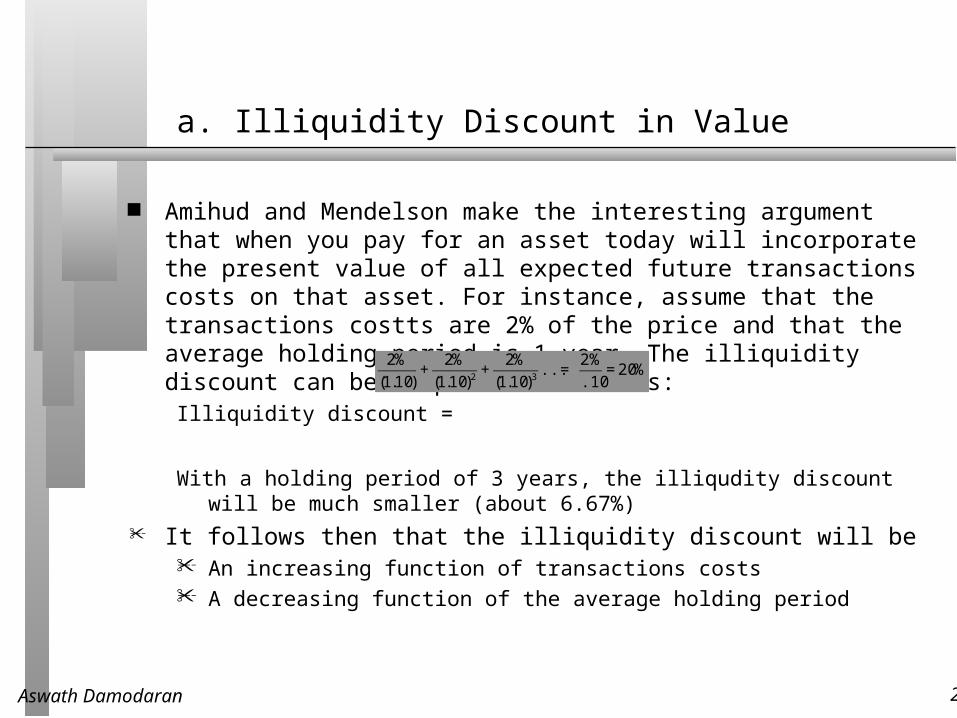
Amihud and Mendelson make the interesting argument that when you pay for an asset today will incorporate the present value of all expected future transactions costs on that asset. For instance, assume that the transactions costts are 2% of the price and that the average holding period is 1 year. The illiquidity discount can be computed as follows:

Illiquidity discount =

With a holding period of 3 years, the illiqudity discount will be much smaller (about 6.67%)

It follows then that the illiquidity discount will be An increasing function of transactions costs A decreasing function of the average holding period

€

2%

(1.10)+

2%

(1.10)2+

2%

(1.10)3... =

2%

.10= 20%

Aswath Damodaran 24

b. Adjusting discount rates for illiquidity

Liquidity as a systematic risk factor• If liquidity is correlated with overall market conditions, less liquid stocks should

have more market risk than more liquid stocks• To estimate the cost of equity for stocks, we would then need to estimate a

“liquidity beta” for every stock and multiply this liquidity beta by a liquidity risk premium.

• The liquidity beta is not a measure of liquidity, per se, but a measure of liquidity that is correlated with market conditions.

Liquidity premiums• You can always add liquidity premiums to conventional risk and return models to

reflect the higher risk of less liquid stocks.• These premiums are usually based upon historical data and reflect what you would

have earned on less liquid investments historically (usually smaller stocks with lower trading volume) relative to more liquid investments. Amihud and Mendelson estimate that the expected return increases about 0.25% for every 1% increase in the bid-ask spread.

Aswath Damodaran 25

c. Illiquidity as a lookback option

Longstaff (1995) presents an upper bound for the option by considering an investor with perfect market timing abilities who owns an asset on which she is not allowed to trade for a period.

In the absence of trading restrictions, this investor would sell at the maximum price that an asset reaches during the time period and the value of the look-back option estimated using this maximum price should be the outer bound for the value of illiquidity. Using this approach,

Aswath Damodaran 26

Valuing the Lookback Option

Aswath Damodaran 27

The Cost of Illiquidity: Empirical EvidenceBond Market

T.Bills versus T.Bonds: The yield on the less liquid treasury bond was higher on an annualized basis than the yield on the more liquid treasury bill, a difference attributed to illiquidity.

Corporate Bonds: A study compared over 4000 corporate bonds in both investment grade and speculative categories, and concluded that illiquid bonds had much higher yield spreads than liquid bonds. This study found that liquidity decreases as they moved from higher bond ratings to lower ones and increased as they move from short to long maturities.

Overall: The consensus finding is that liquidity matters for all bonds, but that it matters more with risky bonds than with safer bonds.

Aswath Damodaran 28

The Cost of Illiquidity:Equity Markets - Cross Sectional Differences

Trading volume: Brennan, Chordia and Subrahmanayam (1998) find that dollar trading volume and stock returns are negatively correlated, after adjusting for other sources of market risk. Datar,

Turnover Ratio: Nair and Radcliffe (1998) use the turnover ratio as a proxy for liquidity. After controlling for size and the market to book ratio, they conclude that liquidity plays a significant role in explaining differences in returns, with more illiquid stocks (in the 90the percentile of the turnover ratio) having annual returns that are about 3.25% higher than liquid stocks (in the 10th percentile of the turnover ratio). In addition, they conclude that every 1% increase in the turnover ratio reduces annual returns by approximately 0.54%.

And it is not a size or price to book effect: Nguyen, Mishra and Prakash (2005) conclude that stocks with higher turnover ratios do have lower expected returns. They also find that market capitalization and price to book ratios, two widely used proxies that have been shown to explain differences in stock returns, do not proxy for illiquidity

Aswath Damodaran 29

Controlled Studies

All of the studies noted on the last page can be faulted because they cannot control for liquidity perfectly. Illiquid stocks are more likely to be in smaller companies that are not held by institutional investors. No matter how carefully a study is done, it will be difficult to categorically state that the observed return differences are due to liquidity.

The studies that carry the most weight for measuring illiquidity, therefore, are studies where we can control for the difference. Usually, they involved shares issued by the same company, with the only difference being that one set of shares is liquid and the other is not. The difference in price can then be attributed entirely to illiquidity.

Aswath Damodaran 30

a. Restricted Stock Studies

Restricted securities are securities issued by a company, but not registered with the SEC, that can be sold through private placements to investors, but cannot be resold in the open market for a one-year holding period, and limited amounts can be sold after that. Restricted securities trade at significant discounts on publicly traded shares in the same company.

• Maher examined restricted stock purchases made by four mutual funds in the period 1969-73 and concluded that they traded an average discount of 35.43% on publicly traded stock in the same companies.

• Moroney reported a mean discount of 35% for acquisitions of 146 restricted stock issues by 10 investment companies, using data from 1970.

• In a recent study of this phenomenon, Silber finds that the median discount for restricted stock is 33.75%.

Many of these older studies were done when the restriction stretched to two years. More recent studies since the change in the holding period come back with lower values for the discount (20-25%).

Aswath Damodaran 31

The problems with restricted stock

There are three statistical problems with extrapolating from restricted stock studies.

• First, these studies are based upon small sample sizes, spread out over long time periods, and the standard errors in the estimates are substantial.

• Second, most firms do not make restricted stock issues and the firms that do make these issues tend to be smaller, riskier and less healthy than the typical firm. This selection bias may be skewing the observed discount.

• Third, the investors with whom equity is privately placed may be providing other services to the firm, for which the discount is compensation.

Bajaj, Dennis, Ferris and Sarin compute a discount of 9.83% for private placements, where there is no illiquidity, and argue that controlling for differences across companies making restricted stock results in an illiqudity discount of 7.23% for restricted stock.

Aswath Damodaran 32

b. Initial Public Offerings.

Aswath Damodaran 33

The problem with IPOs: Side Bets and Other Uncertainties

There are two problems with the IPO studies that make us reluctant to conclude that it is illiquidity.

• The first is the sheer size of the discount suggests that there may be something else going on in these transactions. In particular, these might not be arms length transactions and the sellers of these shares may be getting compensating benefits elsewhere.

• The second is that there may be uncertainty about whether the IPO will go through and if it does, the price at which the company will go public. The discount may reflect how much the sellers are willing to pay to accept a certainty equivalent of a risky cash flow.

Aswath Damodaran 34

c. Companies with different share classes

Some companies have multiple classes of shares in the same market, with some classes being more liquid than others. If there are no other differences (in voting rights or dividends, for instance) across the classes, the difference in prices can be attributed to liquidity.

Chen and Xiong (2001) compare the market prices of the traded common stock in 258 Chinese companies with the auction and private placement prices of the RIS shares and conclude that the discount on the latter is 78% for auctions and almost 86% for private placements.

There are companies in emerging markets with ADRs listed for their stock in the US. The ADRs historically have traded at significant premiums over the domestic listings and some of the difference can be attributed to the higher liquidity of the US market.

Aswath Damodaran 35

Dealing with illiquidity in valuation

If we accept that illiquidity affects value, and both the theory and empirical evidence suggest that it does, the question becomes how best to bring it into the value.

There are three choices:• Estimate the value of the asset as if it were a liquid asset and then discount that

value for illiquidity

• Adjust the discount rates and use a higher discount rate for illiquid companies

• Estimate the illiquidity discount by looking at comparable companies and seeing how much their values are impacted by illiquidity

Aswath Damodaran 36

a. Illiquidity DiscountThe Rule of Thumb approach

In private company valuation, illiquidity is a constant theme that analysts talk about.

All the talk, though, seems to lead to a rule of thumb. The illiquidity discount for a private firm is between 20-30% and does not vary much across private firms.

In our view, this reflects the objective of many appraisers of private companies which has been to get the largest discount that the courts will accept rather than the right illiquidity discount.

Aswath Damodaran 37

Determinants of the Illiquidity Discount

1. Liquidity of assets owned by the firm: The fact that a private firm is difficult to sell may be rendered moot if its assets are liquid and can be sold with no significant loss in value. A private firm with significant holdings of cash and marketable securities should have a lower illiquidity discount than one with factories or other assets for which there are relatively few buyers.

2. Financial Health and Cash flows of the firm: A private firm that is financially healthy should be easier to sell than one that is not healthy. In particular, a firm with strong earnings and positive cash flows should be subject to a smaller illiquidity discount than one with losses and negative cash flows.

3. Possibility of going public in the future: The greater the likelihood that a private firm can go public in the future, the lower should be the illiquidity discount attached to its value. In effect, the probability of going public is built into the valuation of the private firm.

4. Size of the Firm: If we state the illiquidity discount as a percent of the value of the firm, it should become smaller as the size of the firm increases.

5. Control Component: Investing in a private firm is decidedly more attractive when you acquire a controlling stake with your investment. A reasonable argument can be made that a 51% stake in a private business should be more liquid than a 49% stake in the same business.

Aswath Damodaran 38

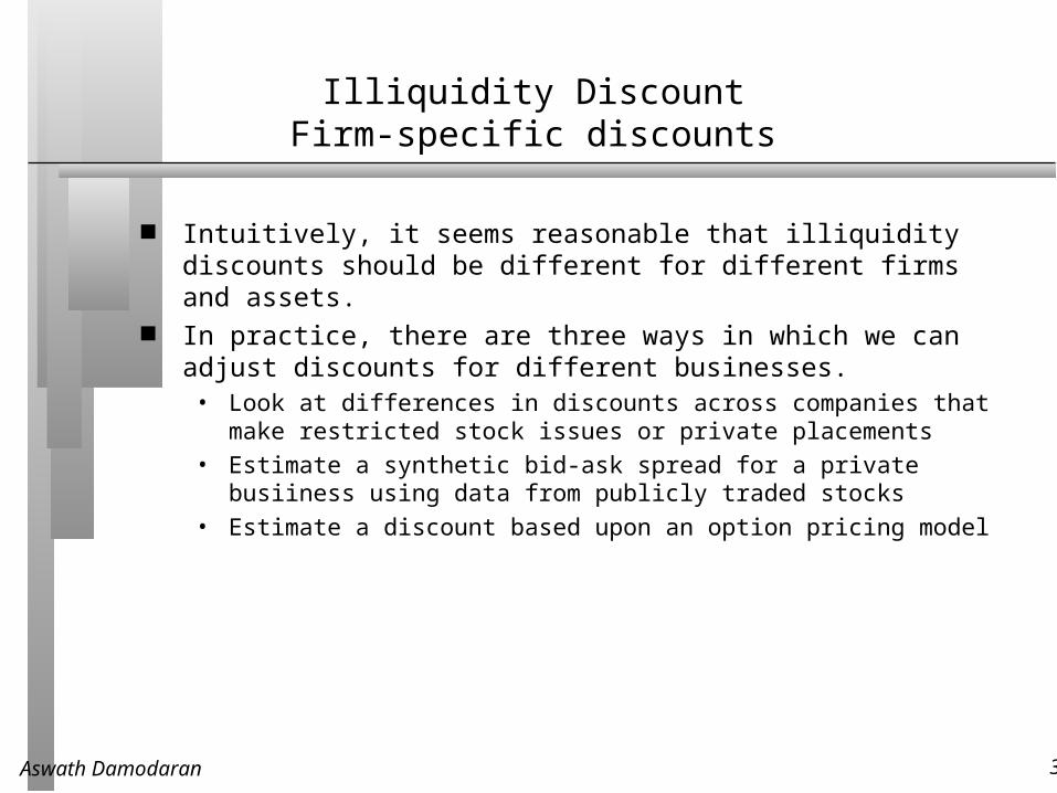
Illiquidity DiscountFirm-specific discounts

Intuitively, it seems reasonable that illiquidity discounts should be different for different firms and assets.

In practice, there are three ways in which we can adjust discounts for different businesses.

• Look at differences in discounts across companies that make restricted stock issues or private placements

• Estimate a synthetic bid-ask spread for a private busiiness using data from publicly traded stocks

• Estimate a discount based upon an option pricing model

Aswath Damodaran 39

1. Exploiting Cross Sectional Differences : Restricted Stock

Silber (1991) develops the following relationship between the size of the discount and the characteristics of the firm issuing the registered stock –

LN(RPRS) = 4.33 +0.036 LN(REV) - 0.142 LN(RBRT) + 0.174 DERN + 0.332 DCUST

where,

RPRS = Relative price of restricted stock (to publicly traded stock)

REV = Revenues of the private firm (in millions of dollars)

RBRT = Restricted Block relative to Total Common Stock in %

DERN = 1 if earnings are positive; 0 if earnings are negative;

DCUST = 1 if there is a customer relationship with the investor; 0 otherwise; Interestingly, Silber finds no effect of introducing a control dummy - set equal

to one if there is board representation for the investor and zero otherwise.

Aswath Damodaran 40

Adjusting the average illiquidity discount for firm characteristics - Silber Regression

The Silber regression does provide us with a sense of how different the discount will be for a firm with small revenues versus one with large revenues.

Consider, for example, two profitable firms that are equal in every respect except for revenues. Assume that the first firm has revenues of 10 million and the second firm has revenues of 100 million. The Silber regression predicts illiquidity discounts of the following:

• For firm with 100 million in revenues: 44.5%

• For firm with 10 million in revenues: 48.9%

• Difference in illiquidity discounts: 4.4% If your base discount for a firm with 10 million in revenues is 25%, the

illiquidity discount for a firm with 100 million in revenues would be 20.6%.

Aswath Damodaran 41

Liquidity Discount and Revenues

Figure 24.1: Illiquidity Discounts: Base Discount of 25% for profitable firm with $ 10 million in revenues

0.00%

5.00%

10.00%

15.00%

20.00%

25.00%

30.00%

35.00%

40.00%

5 10 15 20 25 30 35 40 45 50 100 200 300 400 500 1000Revenues

Discount as % of Value

Profitable firmUnprofitable firm

Aswath Damodaran 42

Application to a private firm: Kristin Kandy

Kristin Kandy is a profitable firm with $ 3 million in revenues. We computed the Silber regression discount using a base discount of 15% for

a healthy firm with $ 10 million in revenues. The difference in illiquidity discount for a firm with $ 10 million in revenues

and a firm with a firm with $ 3 million in revenues in the Silber regression is 2.17%.

Adding this on to the base discount of 15% yields a total discount of 17.17%.

Aswath Damodaran 43

2. An Alternate Approach to the Illiquidity Discount: Bid Ask Spread

As we noted earlier, the bid-ask spread is one very important component of the trading cost on a publicly traded asset. It can be loosely considered to be the illiquidity discount on a publicly traded stock.

Studies have tied the bid-ask spread to• the size of the firm

• the trading volume on the stock

• the degree Regressing the bid-ask spread against variables that can be measured for a

private firm (such as revenues, cash flow generating capacity, type of assets, variance in operating income) and are also available for publicly traded firms offers promise.

Aswath Damodaran 44

A Bid-Ask Spread Regression

Using data from the end of 2000, for instance, we regressed the bid-ask spread against annual revenues, a dummy variable for positive earnings (DERN: 0 if negative and 1 if positive), cash as a percent of firm value and trading volume.

Spread = 0.145 – 0.0022 ln (Annual Revenues) -0.015 (DERN) – 0.016 (Cash/Firm Value) – 0.11 ($ Monthly trading volume/ Firm Value)

You could plug in the values for a private firm into this regression (with zero trading volume) and estimate the spread for the firm.

The synthetic bid-ask spread was computed using the spread regression presented earlier and the inputs for Kristin Kandy (revenues = $3 million, positive earnings, cash/ firm value = 6.56% and no trading)

Spread = 0.145 – 0.0022 ln (Annual Revenues) -0.015 (DERN) – 0.016 (Cash/Firm Value) – 0.11 ($ Monthly trading volume/ Firm Value) = 0.145 – 0.0022 ln (3) -0.015 (1) – 0.016 (0.0696) – 0.11 (0) = 0.1265 or 12.65%

Aswath Damodaran 45

3. Option Based Discount

Liquidity is sometimes modeled as a put option for the period when an investor is restricted from trading. Thus, the illiquidity discount on value for an asset where the owner is restricted from trading for 2 years will be modeled as a 2-year at-the-money put option.

The problem with this is that liquidity does not give you the right to sell a stock at today’s market price anytime over the next 2 years. What it does give you is the right to sell at the prevailing market price anytime over the next 2 years.

One variation that will work is to Assume that you have a disciplined investor who always sells investments, when the price rises 25% above the original buying price. Not being able to trade on this investment for a period (say, 2 years) undercuts this discipline and it can be argued that the value of illiquidity is the product of the value of the put option (estimated using a strike price set 25% above the purchase price and a 2 year life) and the probability that the stock price will rise 25% or more over the next 2 years.

Aswath Damodaran 46

An option based discount for Kristin Kandy

To value illiquidity as an option, we chose arbitrary values for illustrative purposes of an upper limit on the price (at which you would have sold) of 20% above the current value, an industry average standard deviation of 25% and a 1-year trading restriction. The resulting option has the following parameters:

• S = Estimated value of equity = $1,796 million; K = 1,796 (1.20) = $2,155 million; t =1; Riskless rate = 4.5% and = 25%

• Put Option value = $ 354 million The probability that the stock price will increase more than 20% over the next

year was computed from a normal distribution with the average = 16.26% (cost of equity) and standard deviation = 25%.

Z = (20-16.26)/25 = 0.15 N(Z) = 0.5595) Value of liquidity = Value of option to sell at 20% above the current stock

price * Probability that stock price will increase by more than 20% over next year = $354 million * 0.4405 = $156 million

Aswath Damodaran 47

A Comparions of Illiquidity Discounts

Approach Estimated Discount

Liquid ity Adjusted Value

Fixed Discount - Restricted Stock 25.00% $1,347.00

Fixed Discount - Restricted Stock vs Registered Placements 15.00% $1,526.60

15% base discount adjusted for Revenues/Health (Silber) 17.17% $1,487.63 Synthetic Spread 12.65% $1,570.42

Option Based approach (20% upside; Industry variance of 25%; 1 year trading restriction) 8.67% $1,640.24

Aswath Damodaran 48

b. Illiquidity Adjustments to the Discount Rate

1. Add a constant illiquidity premium to the discount rate for all illlquid assets to reflect the higher returns earned historically by less liquid (but still traded) investments, relative to the rest of the market.

• Practitioners attribute all or a significant portion of the small stock premium of 3-4% reported by Ibbotson Associates to illiquidity and add it on as an illiquidity premium. Note, though, that even the smallest stocks listed in their sample are several magnitudes larger than the typical private company and perhaps more liquid.

• An alternative estimate of the premium emerges from studies that look at venture capital returns over long period. Using data from 1984-2004, Venture Economics, estimated that the returns to venture capital investors have been about 4% higher than the returns on traded stocks. We could attribute this difference to illiquidity and add it on as the “illiquidity premium” for all private companies.

2. Add a firm-specific illiquidity premium, reflecting the illiquidity of the asset being valued: For liquidity premiums that vary across companies, we have to estimate a measure of how exposed companies are to liquidity risk. In other words, we need liquidity betas or their equivalent for individual companies.

3. Relate the observed illiquidity premium on traded assets to specific characteristics of those assets. Thus healthier firms with more liquid holdings should have a smaller liquidity premium added on to the discount rate than distressed firms with non-marketable assets.

Aswath Damodaran 49

Illiquidity Discount Rate adjustments for Kristin Kandy

Adding an illiquidity premium of 4% (based upon the premium earned across all venture capital investments) to the cost of equity yields a cost of equity of 20.26% and a cost of capital of 15.17%. Using this higher cost of capital lowers the value of equity in the firm to $1.531 million, about 15.78% lower than the original estimated.

Allowing for the fact that Kristin Kandy is an established business that is profitable would allow us to lower the illiquidity premium to 2% (based upon late stage venture capital investments). This will lower the cost of equity to 18.26%, the cost of capital to 13.77% and result in a value of equity of $1.658 million. The resulting illiquidity discount is 7.66%.

Aswath Damodaran 50

c. Relative Valuation adjustment to value

You can value an illiquid company by finding out the market prices of other companies that were similarly illiquid.

There are two variations that can be used• Use data on private company transactions to estimate the multiple of earnings, book

value or revenues that this company should trade for

• Use data on publicly traded firms and adjust the resulting multiple for illiquidity of a private business

Aswath Damodaran 51

Private Company Transactions Approach: Requirements for Success

There are a number of private businesses that are similar in their fundamental characteristics (growth, risk and cashflows) to the private business being valued.

There are a large enough number of transactions involving these private businesses (assets) and information on transactions prices is widely available.

The transactions prices can be related to some fundamental measure of company performance (like earnings, book value and sales) and these measures are computed with uniformity across the different companies.

Other information encapsulating the risk and growth characteristics of the businesses that were bought is also easily available.

Aswath Damodaran 52

Publicly Traded Company Approach: Variations

Use an illiquidity discount, estimated using the same approaches described earlier, to adjust the multiple: For instance, an analyst who believes that a fixed illiquidity discount of 25% is appropriate for all private businesses would then reduce the public multiple by 25% for private company valuations. An analyst who believes that multiples should be different for different firms would adjust the discount to reflect the firm’s size and financial health and apply this discount to public multiples.

Instead of estimating a mean or median multiples for publicly traded firms, relate the multiples of these firms to the fundamentals of the firms (including size, growth, risk and a measure of illiquidity). The resulting regression can then be used to estimate the multiple for a private business.

Aswath Damodaran 53

Kristin Kandy: Comparable publicly traded firms

Company Name Ticker Symbol EV/ Sales

Operating Margin

Turnover Ratio

Gard enburger Inc GBUR 0.62 0.03 0.65

Paradise Inc PARF 0.33 0.05 0.38

Armanino Foods Dist ARMF 0.59 0.06 0.37

Vita Food Pro ds VSF 0.57 0.02 0.13

Yocream Intl Inc YOCM 0.53 0.07 0.70

Al lergy Research Gro up Inc ALRG 0.72 0.15 0.16

Uni mark Group Inc UNMG 0.55 0.02 0.14

Tofutti Brands TOF 0.81 0.05 0.10

Advanced Nutraceuticals Inc ANII 1.13 0.20 0.26

Sterling Sugars Inc SSUG 0.96 0.15 0.23

Spectru m Organic Products Inc SPOP 0.75 0.02 0.20

Nort hland Cranberr ies Inc NRCNA 0.66 0.10 0.07

Scheid Vi neyards SVIN 1.77 0.25 0.26

Medifast Inc MED 1.41 0.16 0.74

Galaxy Nutritio nal Foods Inc. GXY 1.44 0.09 0.17

Natrol Inc NTOL 0.51 0.06 0.15

Mon terey Gourmet Foods Inc PSTA 0.76 0.01 0.34

ML M acadamia Orchards LP NUT 3.64 0.08 0.39

Gold en Enterprises GLDC 0.50 0.02 0.12

Natural Alternatives Intl Inc. NAII 0.59 0.08 1.31

Rica Foods Inc RCF 0.80 0.06 0.06

Tasty Baking TBC 0.52 0.06 0.39

Scope Ind ustries SCPJ 0.75 0.17 0.15

Bridgford Foods BRID 0.47 0.03 0.07

Poore Brothers SNAK 1.12 0.10 0.70

High Li ner Foods Inc HLF.TO 0.42 0.07 0.23

Seneca Foods 'A ' SENEA 0.38 0.07 0.05

LIFEWAY FOODS LWAY 5.78 0.22 1.95

Seneca Foods 'B' SENEB 0.38 0.07 0.13

FPI L imited FPL.TO 0.40 0.04 0.14

Rocky M ountain Choc Factory RMCF 6.24 0.22 1.65

Calavo Growers Inc. CVGW 0.50 0.04 0.13

MGP In gredients Inc. MGPI 0.55 0.07 1.86

Aswath Damodaran 54

Estimating Kristin Kandy’s value

Regressing EV/Sales ratios for these firms against operating margins and turnover ratios yields the following:

EV/Sales = 0.11 + 10.78 EBIT/Sales + 0.89 Turnover Ratio – 0.67 Beta R2= 45.04%

(0.27) (3.81) (2.81) (1.06)

Kristin Kandy has a pre-tax operating margin of 25%, a zero turnover ratio (to reflect its status as a private company) and a beta (total) of 2.94. This generates an expected EV/Sales ratio of 0.296.

EV/Sales = 0.11 + 10.78 (.25) + 0.89 (0) – 0.67 (2.94) = 0.835 Multiplying this by Kristin Kandy’s revenues of $3 million in the most recent

financial year generates an estimated value for the firm of $2.51 million. This value is already adjusted for illiquidity.

Aswath Damodaran 55

Conclusion

All assets are illiquid, but there are differences in the degree of illiquidity. Illiquidity matters to investors. They pay lower prices and demand higher

returns from less liquid assets than from otherwise similar more liquid assets The effect of illiquidity on value can be estimated in one of three ways

• The value of the asset can be computed as if it were liquid, and then adjusted for illiquidity at the end (as a discount)

• The discount rate used for illiquid assets can be set higher than that used for liquid assets

• The illiquidity effect can be built into value by looking at how similar illiquid companies have been priced in transactions or by adjusting publicly traded company multiples for illiquidity

Aswath Damodaran 56

III. The Not so powerful stockholderThe value of control

Aswath Damodaran

Home Page: www.damodaran.com

E-Mail: adamodar@stern.nyu.edu

Aswath Damodaran 57

Why control matters…

When valuing a firm, the value of control is often a key factor is determining value.

For instance,• In acquisitions, acquirers often pay a premium for control that can be substantial• When buying shares in a publicly traded company, investors often pay a premium

for voting shares because it gives them a stake in control.\• In private companies, there is often a discount atteched to buying minority stakes in

companies because of the absence of control.

Aswath Damodaran 58

What is the value of control?

The value of controlling a firm derives from the fact that you believe that you or someone else would operate the firm differently (and better) from the way it is operated currently.

The expected value of control is the product of two variables: • the change in value from changing the way a firm is operated

• the probability that this change will occur

Aswath Damodaran 59

Determinants of Value

Aswath Damodaran 60

Current Cashflow to FirmEBIT(1-t) : 436 HRK- Nt CpX 3 HRK - Chg WC -118 HRK= FCFF 551 HRKReinv Rate = (3-118)/436= -26.35%; Tax rate = 17.35%Return on capital = 8.72%

Expected Growth from new inv..7083*.0969 =0.0686or 6.86%

Stable Growthg = 4%; Beta = 0.80Country Premium= 2%Cost of capital = 9.92%Tax rate = 20.00% ROC=9.92%; Reinvestment Rate=g/ROC =4/9.92= 40.32%

Terminal Value5= 365/(.0992-.04) =6170 HRK Cost of Equity10.70%Cost of Debt(4.25%+ 0.5%+2%)(1-.20)= 5.40 %

WeightsE = 97.4% D = 2.6%Discount at $ Cost of Capital (WACC) = 10.7% (.974) + 5.40% (0.026) = 10.55%Op. Assets 4312+ Cash: 1787- Debt 141 - Minority int 465=Equity 5,484/ (Common + Preferred shares) Value non-voting share335 HRK/share

Riskfree Rate :HRK Riskfree Rate= 4.25%

+Beta 0.70XMature market premium 4.5%

Unlevered Beta for Sectors: 0.68Firm’s D/ERatio: 2.70%Adris Grupa (Status Quo): 4/2010 Reinvestment Rate 70.83%Return on Capital 9.69%612246365

+ Country Default Spread2%

XRel Equity Mkt Vol1.50On May 1, 2010AG Pfd price = 279 HRKAG Common = 345 HRK

HKR CashflowsLambda0.68XCRP for Croatia (3%)

X

Lambda0.42CRP for Central Europe (3%)Average from 2004-0970.83%Average from 2004-099.69%Year 1 2 3 4 5EBIT (1-t) HRK 466 HRK 498 HRK 532 HRK 569 HRK 608 - Reinvestment HRK 330 HRK 353 HRK 377 HRK 403 HRK 431FCFF HRK 136 HRK 145 HRK 155 HRK 166 HRK 177

Aswath Damodaran 61

A. Value of Gaining Control

Cashflows from existing assetsCashflows before debt payments, but after taxes and reinvestment to maintain exising assets

Expected Growth during high growth periodGrowth from new investmentsGrowth created by making new investments; function of amount and quality of investments

Efficiency GrowthGrowth generated by using existing assets better

Length of the high growth periodSince value creating growth requires excess returns, this is a function of- Magnitude of competitive advantages- Sustainability of competitive advantages

Stable growth firm, with no or very limited excess returns

Cost of capital to apply to discounting cashflowsDetermined by- Operating risk of the company- Default risk of the company- Mix of debt and equity used in financing

Changing ValueHow well do you manage your existing investments/assets?Are you investing optimally forfuture growth?Is there scope for more efficient utilization of exsting assets?

Are you building on your competitive advantages?Are you using the right amount and kind of debt for your firm?

Aswath Damodaran 62

I. Ways of Increasing Cash Flows from Assets in Place

Revenues

* Operating Margin

= EBIT

- Tax Rate * EBIT

= EBIT (1-t)

+ Depreciation- Capital Expenditures- Chg in Working Capital= FCFF

Divest assets thathave negative EBITMore efficient operations and cost cuttting: Higher Margins

Reduce tax rate- moving income to lower tax locales- transfer pricing- risk management

Live off past over- investmentBetter inventory management and tighter credit policies

Aswath Damodaran 63

II. Value Enhancement through Growth

Reinvestment Rate

* Return on Capital

= Expected Growth Rate

Reinvest more inprojectsDo acquisitionsIncrease operatingmarginsIncrease capital turnover ratio

Aswath Damodaran 64

III. Building Competitive Advantages: Increase length of the growth period

Increase length of growth periodBuild on existing competitive advantages

Find new competitive advantages

Brand nameLegal ProtectionSwitching CostsCost advantages

Aswath Damodaran 65

IV. Reducing Cost of Capital

Cost of Equity (E/(D+E) + Pre-tax Cost of Debt (D./(D+E)) = Cost of CapitalChange financing mixMake product or service less discretionary to customers

Reduce operating leverageMatch debt to assets, reducing default risk

Changing product characteristics

More effective advertising

OutsourcingFlexible wage contracts &cost structureSwapsDerivativesHybrids

Aswath Damodaran 66

An Assessment of Ardis Grupa: Where is there most promise?

If you were running Adris Grupa, where do you see the most promise in value enhancement?

Increase cash flows from existing assets Increase growth rate during high growth period (Reinvestment rate = 71%,

Return on capital = 9.69%; Cost of capital = 10.55%; Growth rate = 10.09%) Increase length of growth period (5 years) Reduce cost of capital (Debt ratio = 2.6%) Pay out more of the cash to stockholders (Cash is 30% of overall value)

Aswath Damodaran 67

Ardis : Optimal Capital Structure

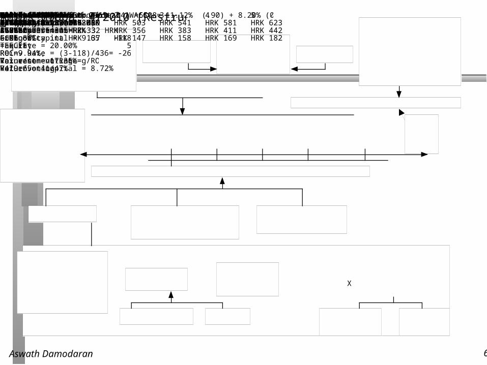
Aswath Damodaran 68

Current Cashflow to FirmEBIT(1-t) : 436 HRK- Nt CpX 3 HRK - Chg WC -118 HRK= FCFF 551 HRKReinv Rate = (3-118)/436= -26.35%; Tax rate = 17.35%Return on capital = 8.72%

Expected Growth from new inv..7083*.01054=0.or 6.86%

Stable Growthg = 4%; Beta = 0.80Country Premium= 2%Cost of capital = 9.65%Tax rate = 20.00% ROC=9.94%; Reinvestment Rate=g/ROC =4/9.65= 41/47%

Terminal Value5= 367/(.0965-.04) =6508 HRK Cost of Equity11.12%Cost of Debt(4.25%+ 4%+2%)(1-.20)= 8.20%

WeightsE = 90 % D = 10 %Discount at $ Cost of Capital (WACC) = 11.12% (.90) + 8.20% (0.10) = 10.55%Op. Assets 4545+ Cash: 1787- Debt 141 - Minority int 465=Equity 5,735

Value/non-voting 334Value/voting 362

Riskfree Rate :HRK Riskfree Rate= 4.25%

+Beta 0.75XMature market premium 4.5%

Unlevered Beta for Sectors: 0.68Firm’s D/ERatio: 11.1%Adris Grupa: 4/2010 (Restructured) Reinvestment Rate 70.83%Return on Capital 10.54%628246367

+ Country Default Spread2%

XRel Equity Mkt Vol1.50On May 1, 2010AG Pfd price = 279 HRKAG Common = 345 HRK

HKR CashflowsLambda0.68XCRP for Croatia (3%)

X

Lambda0.42CRP for Central Europe (3%)Average from 2004-0970.83%e Year 1 2 3 4 5EBIT (1-t) HRK 469 HRK 503 HRK 541 HRK 581 HRK 623 - Reinvestment HRK 332 HRK 356 HRK 383 HRK 411 HRK 442FCFF HRK 137 HRK 147 HRK 158 HRK 169 HRK 182

Increased ROIC to cost of capitalChanged mix of debt and equity tooptimal

Aswath Damodaran 69

Current Cashflow to FirmEBIT(1-t) : 163- Nt CpX 39 - Chg WC 4= FCFF 120Reinvestment Rate = 43/163

=26.46%

Expected Growth in EBIT (1-t).2645*.0406=.01071.07%

Stable Growthg = 3%; Beta = 1.00;Cost of capital = 6.76% ROC= 6.76%; Tax rate=35%Reinvestment Rate=44.37%

Terminal Value5= 104/(.0676-.03) = 2714Cost of Equity8.50%Cost of Debt(4.10%+2%)(1-.35)= 3.97%

WeightsE = 48.6% D = 51.4%Discount at Cost of Capital (WACC) = 8.50% (.486) + 3.97% (0.514) = 6.17%Op. Assets 2,472+ Cash: 330- Debt 1847=Equity 955-Options 0Value/Share $ 5.13

Riskfree Rate :Riskfree rate = 4.10%+Beta 1.10XRisk Premium4%Unlevered Beta for Sectors: 0.80Firm’s D/ERatio: 21.35%Mature riskpremium4%

Country Equity Prem0%

Blockbuster: Status Quo Reinvestment Rate 26.46%Return on Capital4.06%Term Yr184 82102

1 2 3 4 5EBIT (1-t) $165 $167 $169 $173 $178 - Reinvestment $44 $44 $51 $64 $79 FCFF $121 $123 $118 $109 $99

Aswath Damodaran 70

Current Cashflow to FirmEBIT(1-t) : 249- Nt CpX 39 - Chg WC 4= FCFF 206Reinvestment Rate = 43/249

=17.32%

Expected Growth in EBIT (1-t).1732*.0620=.01071.07%

Stable Growthg = 3%; Beta = 1.00;Cost of capital = 6.76% ROC= 6.76%; Tax rate=35%Reinvestment Rate=44.37%

Terminal Value5= 156/(.0676-.03) = 4145Cost of Equity8.50%Cost of Debt(4.10%+2%)(1-.35)= 3.97%

WeightsE = 48.6% D = 51.4%Discount at Cost of Capital (WACC) = 8.50% (.486) + 3.97% (0.514) = 6.17%Op. Assets 3,840+ Cash: 330- Debt 1847=Equity 2323-Options 0Value/Share $ 12.47

Riskfree Rate :Riskfree rate = 4.10%+Beta 1.10XRisk Premium4%Unlevered Beta for Sectors: 0.80Firm’s D/ERatio: 21.35%Mature riskpremium4%

Country Equity Prem0%

Blockbuster: Restructured Reinvestment Rate 17.32%Return on Capital6.20%Term Yr280124156

1 2 3 4 5EBIT (1-t) $252 $255 $258 $264 $272 - Reinvestment $44 $44 $59 $89 $121 FCFF $208 $211 $200 $176 $151

Aswath Damodaran 71

B. The Probability of Changing Control

The probability of changing management will be different across different companies and will vary across different markets. In general, the more power stockholders have and the stronger corporate governance systems are, the greater is the probability of management change for any given firm.

The probability of changing management will change over time as a function of legal changes, market developments and investor shifts.

Aswath Damodaran 72

Mechanisms for changing management

Activist investors: Some investors have been willing to challenge management practices at companies by offering proposals for change at annual meetings. While they have been for the most part unsuccessful at getting these proposals adopted, they have shaken up incumbent managers.

Proxy contests: In proxy contests, investors who are unhappy with management try to get their nominees elected to the board of directors.

Forced CEO turnover: The board of directors, in exceptional cases, can force out the CEO of a company and change top management.

Hostile acquisitions: If internal processes for management change fail, stockholders have to hope that another firm or outside investor will try to take over the firm (and change its management).

Aswath Damodaran 73

Determinants of Likelihood of Change: Institutional Factors

Capital restrictions: In markets where it is difficult to raise funding for hostile acquisitions, management change will be less likely. Hostile acquisitions in Europe became more common after the corporate bond market developed.

State Restrictions: Some markets restrict hostile acquisitions for parochial (France and Dannon, US and Unocal), political (Pennsylvania’s anti-takeover law to protect Armstrong Industries), social (loss of jobs) and economic reasons (prevent monopoly power).

Inertia and Conflicts of Interest: If financial service institutions (banks and investment banks) have ties to incumbent managers, it will become difficult to change management.

Aswath Damodaran 74

Determinants of the Likelihood of Change: Firm-specific factors

Anti-takeover amendments: Corporate charters can be amended, making it more difficult for a hostile acquirer to acquire the company or dissident stockholders to change management.

Voting Rights: Incumbent managers get voting rights which are disproportional to their stockholdings, by issuing shares with no voting rights or reduced voting rights to the public.

Corporate Holding Structures: Cross holdings and Pyramid structures are designed to allow insiders with small holdings to control large numbers of firms.

Large Stockholders as managers: A large stockholder (usually the founder) is also the incumbent manager of the firm.

Aswath Damodaran 75

Why the probability of management changing shifts over time….

Corporate governance rules can change over time, as new laws are passed. If the change gives stockholders more power, the likelihood of management changing will increase.

Activist investing ebbs and flows with market movements (activist investors are more visible in down markets) and often in response to scandals.

Events such as hostile acquisitions can make investors reassess the likelihood of change by reminding them of the power that they do possess.

Aswath Damodaran 76

Estimating the Probability of Change

You can estimate the probability of management changes by using historical data (on companies where change has occurred) and statistical techniques such as probits or logits.

Empirically, the following seem to be related to the probability of management change:

• Stock price and earnings performance, with forced turnover more likely in firms that have performed poorly relative to their peer group and to expectations.

• Structure of the board, with forced CEO changes more likely to occur when the board is small, is composed of outsiders and when the CEO is not also the chairman of the board of directors.

• Ownership structure; forced CEO changes are more common in companies with high institutional and low insider holdings. They also seem to occur more frequently in firms that are more dependent upon equity markets for new capital.

• Industry structure, with CEOs more likely to be replaced in competitive industries.

Aswath Damodaran 77

Assessing the Probability of Control Change at Adris Grupa

On the minus side, the company has voting and non-voting shares and the controlling family is firmly in control of the firm (as attested to by their holding of the voting shares and their presence in top management and the board of directors).

On the plus side, the non-voting shareholders have been provided with full tag-along rights in a takeover, entitling them to a fair share of the gains.

Bottom line: The probability of control changing in a hostile takeover is close to zero. The probability of control changing in a friendly takeover is much higher.

Aswath Damodaran 78

Manifestations of the Value of Control

Hostile acquisitions: In hostile acquisitions which are motivated by control, the control premium should reflect the change in value that will come from changing management.

Valuing publicly traded firms: The market price for every publicly traded firm should incorporate an expected value of control, as a function of the value of control and the probability of control changing.

Market value = Status quo value + (Optimal value – Status quo value)* Probability of management changing

Voting and non-voting shares: The premium (if any) that you would pay for a voting share should increase with the expected value of control.

Minority Discounts in private companies: The minority discount (attached to buying less than a controlling stake) in a private business should be increase with the expected value of control.

Aswath Damodaran 79

1. Hostile Acquisition: Example

In a hostile acquisition, you can ensure management change after you take over the firm. Consequently, you would be willing to pay up to the optimal value.

As an example, Blockbuster was trading at $9.50 per share in July 2005. The optimal value per share that we estimated as $ 12.47 per share. Assuming that this is a reasonable estimate, you would be willing to pay up to $2.97 as a premium in acquiring the shares.

Issues to ponder:• Would you automatically pay $2.97 as a premium per share? Why or why not?

• What would your premium per share be if change will take three years to implement?

Aswath Damodaran 80

Hostile Acquisitions: Implications

a. The value of control will vary across firms: Since the control premium is the difference between the status-quo value of a firm and its optimal value, it follows that the premium should be larger for poorly managed firms and smaller for well managed firms.

b. There can be no rule of thumb on control premium: Since control premium will vary across firms, there can be no simple rule of thumb that applies across all firms. The notion that control is always 20-30% of value cannot be right.

c. The control premium should vary depending upon why a firm is performing badly: The control premium should be higher when a firm is performing badly because of poor management decisions than when a firm’s problems are caused by external factors over which management has limited or no control.

d. The control premium should be a function of the ease of making management changes: Not all changes are easy to make or quick to implement. It is far easier to change the financing mix of an under levered company than it is to modernize the plant and equipment of a manufacturing company with old and outdated plants.

Aswath Damodaran 81

Hostile Acquisitions: Evidence of a control effect

a. Premiums paid for target firms in acquisitions: While the average premium paid for target firms in acquisitions in the United States has been between 20 and 30% in the 1980s and 1990s, the premiums tend to be slightly higher for hostile acquisitions. In addition, bidding firm returns which tend to be negligible or slightly negative across all acquisitions are much more positive on hostile acquisitions.

b. Target firm characteristics: Target firms in hostile takeovers have earned a 2.2% lower return on equity, on average, than other firms in their industry; they have earned returns for their stockholders that are 4% lower than the market; and only 6.5% of their stock is held by insiders. The typical target firm is characterized by poor project choice and stock price performance as well as low insider holdings.

c. Post-acquisition actions: contrary to popular view, most hostile takeovers are not followed by the acquirer stripping the assets of the target firm and leading it to ruin. Instead, target firms refocus on their core businesses and often improve their operating performance.

Aswath Damodaran 82

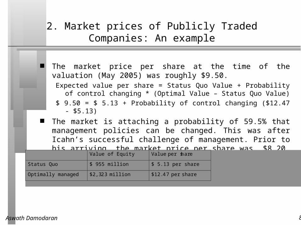
2. Market prices of Publicly Traded Companies: An example

The market price per share at the time of the valuation (May 2005) was roughly $9.50.

Expected value per share = Status Quo Value + Probability of control changing * (Optimal Value – Status Quo Value)

$ 9.50 = $ 5.13 + Probability of control changing ($12.47 - $5.13) The market is attaching a probability of 59.5% that management policies can

be changed. This was after Icahn’s successful challenge of management. Prior to his arriving, the market price per share was $8.20, yielding a probability of only 41.8% of management changing.

Value of Equity Value per share

Status Quo $ 955 million $ 5.13 per share

Optimally mana ged $2,323 million $12.47 per share

Aswath Damodaran 83

Market Prices for Publicly Traded Firms: Implications

a. Paying a premium over the market price can result in over payment: In a firm where the market already assumes that management will be changed and builds it into the stock price, acquirers should be wary of paying a premium on the current market price even for a badly managed firm.

b. Anything that causes market perception of the likelihood of management change to shift can have large effects on all stocks. A hostile acquisition of one company, for instance, may lead investors to change their assessments of the likelihood of management change for all companies and to an increase in stock prices.

c. Poor corporate governance = Lower stock prices: Stock prices in a market where corporate governance is effective will reflect a high likelihood of change for bad management and a higher expected value for control. In contrast, it is difficult, if not impossible, to dislodge managers in markets where corporate governance is weak. Stock prices in these markets will therefore incorporate lower expected values for control. The differences in corporate governance are likely to manifest themselves most in the worst managed firms in the market.

Aswath Damodaran 84

Market Price for Publicly Traded Firms: Evidence of a control effect

a. Hostile Acquisitions: If the prices of all stocks reflect the expected value of control, any actions that make hostile acquisitions more or less likely will affect stock prices. When Pennsylvania passed its anti-takeover law in 1989, Pennsylvania firms saw their stock prices decline 6.90%.

b. Management Changes: In badly managed firms, a forced CEO turnover with an outside successor has the most positive consequences, especially when the outsider is viewed as someone capable of changing the way the firm is run.

c. Corporate Governance:

• Gompers, Ishi and Metrick found that the stocks with the weakest stockholder power earned 8.4% less in annual returns than stockholders with the strongest stockholder power. They also found that an increase of 1% in the poor governance index translated into a decline of 2.4% in the firm’s Tobin’s Q, which is the ratio of market value to replacement cost.

• Bris and Cabolis look at target firms in 9277 cross-border mergers, where the corporate governance system of the target is in effect replaced by the corporate governance system of the acquirer. They find that the Tobin’s Q increases for firms in an industry when a firm or firms in that industry are acquired by foreign firms from countries with better corporate governance

Aswath Damodaran 85

3. Voting and Non-voting Shares: An Example

The value of a voting share derives entirely from the capacity you have to change the way the firm is run.

In this case, we have two values for Adris Grupa’s Equity.

Status Quo Value of Equity = 5,469 million HKR

All shareholders, common and preferred, get an equal share of the status quo value.

Value for a non-voting share = 5469/(9.616+6.748) = 334 HKR/share

Optimal value of Equity = 5,735 million HKR

Value of control at Adris Grupa = 5,735 – 5469 = 266 million HKR

Only voting shares get a share of this value of control

Value per voting share =334 HKR + 266/9.616 = 362 HKR

Aswath Damodaran 86

Voting and Non-voting Shares: Implications

a. The difference between voting and non-voting shares should go to zero if there is no chance of changing management/control. If there are relatively few voting shares, held entirely by insiders, the probability of management change may very well be close to zero and voting shares should trade at the same price as non-voting shares.

b. Other things remaining equal, voting shares should trade at a larger premium on non-voting shares at badly managed firms than well-managed firms. In a badly managed firm, the expected value of control is likely to be higher.

c. Other things remaining equal, the smaller the number of voting shares relative to non-voting shares, the higher the premium on voting shares should be. The expected value of control is divided by the number of voting shares to get the premium; the smaller that number, the greater the value per share.

d. Other things remaining equal, the greater the percentage of voting shares that are available for trading by the general public (float), the higher the premium on voting shares should be. When voting shares are predominantly held by insiders, the probability of control changing is small and so is the expected value of control.

e. Any event that illustrates the power of voting shares relative to non-voting shares is likely to affect the premium at which all voting shares trade.

Aswath Damodaran 87

4. Minority Discount: An example

Assume that you are valuing Kristin Kandy, a privately owned candy business for sale in a private transaction. You have estimated a value of $ 1.6 million for the equity in this firm, assuming that the existing management of the firm continues into the future and a value of $ 2 million for the equity with new and more creative management in place.

• Value of 51% of the firm = 51% of optimal value = 0.51* $ 2 million = $1.02 million

• Value of 49% of the firm = 49% of status quo value = 0.49 * $1.6 million = $784,000

Note that a 2% difference in ownership translates into a large difference in value because one stake ensures control and the other does not.

Aswath Damodaran 88

Minority Discount: Implications

a. The minority discount should vary inversely with management quality: If the minority discount reflects the value of control (or lack thereof), it should be larger for firms that are poorly run and smaller for well-run firms.

b. Control may not always require 51%: While it is true that you need 51% of the equity to exercise control of a private firm when you have only two co-owners, it is possible to effectively control a firm with s smaller proportion of the outstanding stock when equity is dispersed more investors.

c. The value of an equity stake will depend upon whether it provides the owner with a say in the way a firm is run: Many venture capitalists play an active role in the management of the firms that they invest in and the value of their equity stake should reflect this power. In effect, the expected value of control is built into the equity value. In contrast, a passive private equity investor who buys and holds stakes in private firms, without any input into the management process, should value her equity stakes at a lower value.

Aswath Damodaran 89

To conclude…

The value of control in a firm should lie in being able to run that firm differently and better. Consequently, the value of control should be greater in poorly performing firms.

The market value of every firm reflects the expected value of control, which is the product of the probability of management changing and the effect on value of that change.

With companies with voting and non-voting shares, the premium on voting shares should reflect the expected value of control. If the probability of control changing is small and/or the value of changing management is small (because the company is well run), the expected value of control should be small and so should the voting stock premium.

In private company valuation, the discount applied to minority blocks should be a reflection of the value of control.