sustainability

Article

Asset Allocation Model for a Robo-Advisor Using theFinancial Market Instability Index andGenetic Algorithms

Wonbin Ahn 1, Hee Soo Lee 2, Hosun Ryou 3 and Kyong Joo Oh 3,*1 Center of Bionics, Korea Institute of Science and Technology, Seoul 02792, Korea; wbahn@kist.re.kr2 Department of Business Administration, Sejong University, Seoul 05006, Korea; heesoo@sejong.ac.kr3 Department of Industrial Engineering, Yonsei University, Seoul 03722, Korea; ryouho@yonsei.ac.kr* Correspondence: johanoh@yonsei.ac.kr; Tel.: +82-2-2123-5720

Received: 6 December 2019; Accepted: 18 January 2020; Published: 23 January 2020�����������������

Abstract: There has been a growing demand for portfolio management using robo-advisors, andhence, research on the automation of portfolio composition has been increasing. In this study,we propose a model that automates the portfolio structure by using the instability index of thefinancial time series and genetic algorithms (GAs). We use the instability index to filter the investmentassets and optimize the threshold value used as a filtering criterion by applying a GA. For an empiricalanalysis, we use stocks, bonds, commodities exchange traded funds (ETFs), and exchange rate.We compare the performance of our model with that of risk parity and mean-variance models andfind our model has better performance. Several additional experiments with our model using variousinternal parameters are conducted, and the proposed model with a one-month test period after oneyear of learning is found to provide the highest Sharpe ratio.

Keywords: financial market instability index; genetic algorithm; asset allocation; exchangetraded funds

1. Introduction

Interest in robo-advisors is growing with FinTech trends. FinTech, a compound of finance andtechnology, has a large impact on various industries as well as the financial industry. As one ofthe most important FinTech developments, robo-advisors are being treated as representative of thenext-generation business model in the area of portfolio management by the investor community [1,2].On behalf of human investment professionals, robo-advisors provide online investment advisory servicefor portfolio management according to individual investment propensity and investment purpose withbig data analysis and advanced algorithm-based automation system. In fact, robo-advisors are not anentirely new technique, but the terminology is new. The core of the robo-advisors is the composition ofinvestments in a portfolio that is mainly based on exchange traded funds (ETFs). An ETF is a typeof fund that owns the underlying assets such as stocks, bonds or commodities and is traded like acommon stock on a stock exchange with relatively low transaction costs [3]. Empirical research onrobo-advisors has been steadily progressing with technology development. Recent developments ininformation and communication technology (ICT) and artificial intelligence have defined new termsand become a domain of the robo-advisor [4,5]. Several studies show better portfolio managementperformance using artificial intelligence than using various existing strategies [6–8].

As financial markets are constantly evolving with sophisticated techniques, the classical financialtheories or traditional models are no longer effective to understand the financial market mechanism andconstruct efficient portfolios. Since the mean-variance model by Markowitz, the asset allocation modelfor optimal portfolio has evolved steadily [9]. The mean-variance model has been extensively used

Sustainability 2020, 12, 849; doi:10.3390/su12030849 www.mdpi.com/journal/sustainability

Sustainability 2020, 12, 849 2 of 15

for theoretical and empirical studies [10,11]. Since the 1960s, the capital asset pricing model (CAPM)and a model that eliminates unsystematic risk from diversified investment were developed [12–14].The CAPM, which find expected return of asset based on many assumptions, has been criticizedbecause it does not fit real market conditions [15]. Since then, the multi-factor model using otherfactors in addition to market return are introduced, and the Black–Litterman model which reflectsinvestor’s market prospects was introduced for constructing a portfolio [15–17].

The other noteworthy model is the risk parity model, which is gradually replacing existingmodels. The risk parity model has many advantages over the previous models. This model allowsinvestors to focus more on risk than other factors. It effectively constructs a more diversified portfolioand shows good performance in backtesting [18–21]. This result seems to be possible because themodel shows lower drawdown and volatility than existing models. However, some have arguedthat the risk parity strategy is affected by interest rates, lacks consideration of future returns, andrequires leveraging low-risk assets. The weights on each asset included in a portfolio can be changedsignificantly depending on risk measurement. Furthermore, the risk parity strategy does not reflect theinvestor’s special circumstances efficiently. In contrast, a robo-advisor needs to reflect investors’ riskpreferences more properly for portfolio management regardless of leverage. Indeed, a model that canselect assets considering investors’ risk preference is more efficient for portfolio management.

The classical financial theories or traditional models are no longer effective to understand thefinancial market mechanism and construct efficient portfolios because financial markets are constantlyevolving with sophisticated techniques. The purpose of this research is to develop an asset allocationmodel for a robo-advisor using more advanced techniques and compare its performance with those oftraditional models. The model proposed in this paper focuses on asset instability. This model usesmarket indices to measure the degree of instability of financial time series data, compares them tothresholds, and manages risk by eliminating unstable assets. The degree of instability is measured by ap-value that is used to determine the weight of each asset included in a portfolio. Genetic algorithmsare used to optimize thresholds to determine the degree of instability. By comparing with the riskparity model and the mean-variance model, we confirm that the proposed model provides higherprofitability and stability [22,23]. The significant advantage of the proposed model is that it can reflectinvestors’ propensity to invest in various ways by adjusting this threshold. We can increase the shareof assets with high instability for investors who prefer risk, whereas we can increase the proportion ofstable assets for investors who prefer stability. A general role of a robo-advisor is to provide financialadvice or investment management based on mathematical rules or algorithm. In this sense, our assetallocation model can be used as a portfolio management algorithm or an automated investment adviceby a robo-advisor.

For empirical analysis, we use ETFs traded in Korean markets. Many recent portfolio investmentsfocus on investing in ETFs. Before ETFs are traded on the market, it is difficult to manage the risks of aportfolio because a lot of capital is required to make a diversified portfolio. However, with the adventof ETFs, it is possible to make a fully diversified portfolio even at low cost.

The composition of this paper is as follows. In Section 2, we review the algorithms and theoriesused in the proposed model and describe how to derive the iFMII (integrated financial market instabilityindex) that identifies instability. We also discuss the risk parity model and the genetic algorithms usedfor threshold optimization and describe the components of the proposed model. In Section 3, we reportempirical results and compare the performance of our model with that of other models. Section 4concludes our paper.

Sustainability 2020, 12, 849 3 of 15

2. Materials and Methods

2.1. Literature Review

2.1.1. p-Value Derived from the iFMII

The p-value indicating the degree of instability has been derived from the iFMII. In fact, theinstability index was first introduced as the iSMII (integrated stock market instability index), but it wasexpanded to the iFMII so that it is not limited to the stock market [24]. The iFMII considers time seriesdata to be linear or nonlinear. For the nonlinear model, nonparametric nearly stationary autoregressive(NNSAR) model with artificial neural networks (ANN) is used. ANN is one of the widely appliedmodels with nonlinear time series. For the linear model, autoregressive (AR) model is used.

As a first step, a stable interval of the time series between certain values is determined. Once theinterval is determined, linear and nonlinear models are constructed based on the stable interval. Then,the time series included in the remaining interval is predicted by the model constructed in the stableinterval. To determine the order of constructed model, sample partial autocorrelation function (SPACF)is used.

The linear FMII (financial market instability index) and the nonlinear FMII are calculated as thedifference between the predicted value and the actual value. Because the model is constructed basedon a stable section, the larger the error, the more unstable the value is. The two derived FMIIs arecombined using the Bayesian averaging method to produce the iFMII. It is empirically found that thecombined index with approximately 50% of each FMII best reflects the degree of instability. The p-valueof each FMII is obtained rank of the error in descending order, which implies that the higher the errorvalue (or the lower the rank of an error), the lower the p-value. The two p-values obtained from thelinear and nonlinear FMIIs are also combined to same weight as when calculating the iFMII to producethe p-value of the iFMII called the ip-value. Previous studies have shown that an ip-value lower than0.2 indicates a very unstable condition in the Korean stock market [24]. In this paper, we propose tooptimize the threshold value for unstable conditions and determine whether a 0.2 threshold valueis appropriate.

2.1.2. Risk Parity Model

To use the mean-variance model to make an efficient portfolio, the expected return of each asset,the covariance matrix, and the risk aversion factor of the investor are required [9,16]. The covariancematrix includes the volatility of each asset and covariances between all possible pairs of each assetincluded in the portfolio. Expected return, volatility, and correlation are estimated by various methods,but the most controversial variable is the expected return. The expected return has the greatest impacton asset allocation decisions depending on the estimation method, such as using historical figures andassumptions imposed for estimation.

To overcome these weaknesses, various alternatives have been proposed. One of them is therisk parity model that requires only the covariance matrix [25,26]. The risk parity model constitutesa portfolio so that each asset (or security) has the same risk contribution to the total portfolio risk.In this sense, the risk parity model is considered a model for distributing risks rather than a model forconstructing an efficient portfolio. In this paper, the historical standard deviation of each asset is usedas the volatility measure, and the assets in a portfolio are allocated proportionally to the reciprocal ofthe volatility, which is also known as naïve model of risk parity [27–30].

2.1.3. Genetic Algorithms

A genetic algorithm is an optimization methodology that is based on the principles of Darwinianevolution [31–34]. The algorithm is mainly used to find solutions to nonlinear optimization problemsusing evolutionary rules such as crossover, selection, and mutation. Before applying the algorithm,all candidates (chromosomes) for solutions are usually converted into a binary structure, and the

Sustainability 2020, 12, 849 4 of 15

objective (fitness) function, which represents the goal of the problem and is used to calculate fitnessscore, should be constructed. A set of chromosomes is called a population, and each populationis numbered as the nth generation. Moving on to the next generation, the evolutionary rules areimplemented based on the fitness scores of chromosomes, which measure how well chromosomes fit theproblem. Typically, chromosomes that have higher fitness scores have higher probability to be parentsfor crossover according to a selection rule. A crossover rule is a way to create better chromosomesby mixing two different chromosomes, and a mutation rule randomly selects and changes genes ofchromosomes. By repeating this process, chromosomes gradually fit the objective function and arecloser to the optimal solution [35,36].

In this study, a GA is used to optimize the thresholds of asset filtering in a portfolio. The thresholdset of each asset in a portfolio is treated as a variable, and the maximization of the Sharpe ratio withzero risk-free rate over the past period is used as an objective function. The Sharpe ratio which iswidely used in finance to measure an asset’s performance is defined as the average return earnedmore than the risk-free rate per unit of volatility or total risk. For the operators on the GA, rank-basedselection and uniform crossover with 0.5 crossover rate are used. Mutation method is performedrandomly by variables individually with 0.1 mutation rate. By rank-ordered replacement method, theworst solutions are replaced with new possible solutions created by operators. The GA stops onlywhen the fitness value has not improved at least 0.01% during last 20,000 trials. The larger the trials,the more likely it is to obtain a globally optimized solution, but complexity increases exponentially infinding an optimal threshold. Therefore, the empirical analysis is usually carried out using a reasonablestopping condition in the process of finding an optimal solution.

2.2. Proposed Model

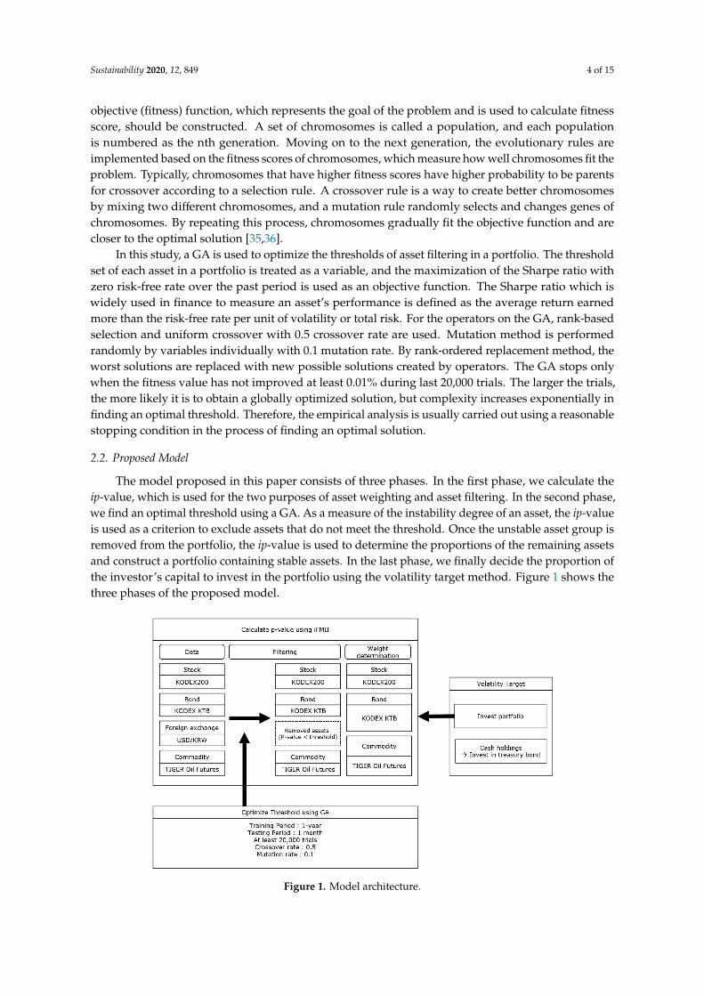
The model proposed in this paper consists of three phases. In the first phase, we calculate theip-value, which is used for the two purposes of asset weighting and asset filtering. In the second phase,we find an optimal threshold using a GA. As a measure of the instability degree of an asset, the ip-valueis used as a criterion to exclude assets that do not meet the threshold. Once the unstable asset group isremoved from the portfolio, the ip-value is used to determine the proportions of the remaining assetsand construct a portfolio containing stable assets. In the last phase, we finally decide the proportion ofthe investor’s capital to invest in the portfolio using the volatility target method. Figure 1 shows thethree phases of the proposed model.

Figure 1. Model architecture.

Sustainability 2020, 12, 849 5 of 15

2.2.1. Phase 1: Calculate the ip-Value from the IFMII

The FMII value for each asset is obtained by constructing linear and nonlinear models for thetime series data included in a stable interval. For a given time series of ith asset Yi1, Yi2, · · · , Yin, theNNSAR model with order k and the error term ei,t is presented in Equation (1).

Yi,t = ft(Yi,t−1, Yi,t−2, · · · , Yi,t−k

)+ ei,t, t = 1, 2, · · · , n (1)

The AR model with order k and the error term ei,t is presented in Equation (2).

Yi,t = ∅i,1Yi,t−1 +∅i,2Yi,t−2 + · · ·+∅i,kYi,t−k + ei,t, t = 1, 2, · · · , n (2)

The FMII value for each asset is the error between the predicted value from the constructed modeland the actual value. We use the mean absolute percentage error type (MAPE) presented in Equation (3)to calculate the error.

MAPE(t) =1n

n−1∑i=0

∣∣∣Yt−i − Yt−i∣∣∣

Yt−i× 100 (3)

where Yt−i is the predicted value and the Yt−i is actual value. FMII1 is derived from the linear model,and FMII2 is derived from the nonlinear model. Then, the p-value is calculated for each FMII value,and the two p-values are combined to determine the final ip-value for the asset.

First, we determine a stable interval for each asset. A stable interval means a period in which themovement of the asset’s time series data appears to be a normal (or stationary) time series. Generally,an interval where the time series is not volatile and moves within a certain box is selected as a stableinterval. After selecting the stable interval and calculating FMII1 and FMII2 for each asset, the p-valueof FMII1 and FMII2 for each asset is obtained by dividing the rank of its FMII value in descendingorder by the total number of predictions. We first calculate the p-value for the linear model. For a giveninterval, we check the sample autocorrelation function (SACF) to determine whether the time series inthe interval is abnormal (or nonstationary). Then, we use the nonstationary linear AR model for theprediction of an abnormal time series. The order of the AR and ANN model is determined througha SPACF. The AR formula is constructed using the determined order, and the FMII1 of each asset isderived. In this paper, the SPACF cuts off at a lag of 2 because it is the first time that the SPACF isbetween −0.2 and 0.2. Therefore, we can present our AR(2) and ANN models as Equations (4) and (5),respectively. The error terms for (5) are fitted by using AR(1) after ANN model constructed

Yi,t = ∅i,1Yi,t−1 +∅i,2Yi,t−2 + ei,t, t = 1, 2, · · · , n (4)

Yi,t = ft(Yi,t−1, Yi,t−2) + ei,t, t = 1, 2, · · · , n (5)

When asset movements are nonlinear, an ANN is used to estimate and predict nonlinear timeseries. The ANN derives FMII2 using the commonly used backpropagation (BPN) algorithm andmulti-layer perceptron (MLP) architecture with 2 × 3 × 1 for financial data analysis. In this paper.The p-value from the linear model (FMII1) and the nonlinear model (FMII2) is calculated by Equation (6)and they are combined with an equal weight to calculate the ip-value of the asset. The derived ip-valuehas a value between 0 and 1, and values closer to 0 mean more unstable and those closer to 1 indicatemore stable. This value is used for two purposes in the next step.

p− value =the rank of FMII in decending order

the total number of prediction(6)

2.2.2. Phase 2: Determine the Allocation of Assets

The allocation of assets uses the ip-value calculated in Section 3.1. First, we use ip-value to filterthe assets. If the ip-value is lower than a certain value, it is excluded from the portfolio because it

Sustainability 2020, 12, 849 6 of 15

is considered unusual and unstable. The second use of ip-value is to determine the weight of eachasset in the portfolio. The weight is obtained by dividing the ip-value of each asset by the total sum ofthe ip-value of all assets in the portfolio. For example, the ip-values of three assets in a portfolio, A1,A2, and A3, are 0.3, 0.8, and 0.1, respectively, and the threshold is 0.2. Then, A3 is excluded from theportfolio, and the investment weight for each asset is as follows:

A1 = 0.3/(0.3 + 0.8 + 0) = 0.27

A2 = 0.8/(0.3 + 0.8 + 0) = 0.73

A3 = 0

The determination of the asset weight as mentioned above requires a threshold value for theip-value. In a previous study, the threshold value for the p-value is reported as 0.2 for the Koreanstock market, but this value is not always appropriate [24]. In this paper, a GA is used to determine anappropriate threshold value with a population size, crossover rate and mutation rate of 1000, 0.5 and0.06, respectively. The learning section sets a certain period of time in the past where the optimizedip-value is found. The chromosome is a linear form of the ip-value threshold for each asset, and theobjective function is to maximize the Sharpe ratio of index returns over the past period. We use theoptimized ip-value threshold from the GA to remove unstable assets and determine the asset weight ofa portfolio for the next period.

2.2.3. Phase 3: Volatility Target

Once the asset weights in the portfolio have been obtained, investors must determine theproportion of their capital to invest in the portfolio. We use the volatility target method to determinethe portfolio investment proportion. First, the portfolio volatility is calculated using the volatility,weight of each asset, and the correlation coefficient between asset returns in the portfolio. Then, if theportfolio volatility is larger than target volatility, the capital proportion of investing in the portfolio isobtained by dividing the target volatility by the portfolio volatility. The investor’s capital, other thanportfolio investment, is assumed to be invested in bond. Finally, the investor’s total return is generatedby the portfolio returns and the bond returns.

2.3. Application of the Proposed Model to Build a Robo-Advisor

A robo-advisor is created by a team of experts in financial advice, investment management,and tech product development. The procedure of building a robo-advisor largely consists of threesteps. A robo-advisor framework in Figure 2 describes the procedure of building a robo-advisor. In thefirst step shown in panel 1 of Figure 2, a model for identifying customer propensity is developed whereclient survey is conducted, and clients are classified depending on their status and risk preferences.In the second step shown in panels 2–5 of Figure 2, an optimized portfolio is constructed by judgingmarket status, measuring price volatility, and clustering ETF by risk level. As the last step shown inpanel 6 of Figure 2, pattern matching trading system is developed for making actual trades. ComparingFigures 1 and 2, the proposed model in this paper can be applied to the second step of building arobo-advisor as the proposed asset allocation model consisting of three phases can be used to make anoptimized portfolio. In other words, Figure 1 is related to panels 2–5 of Figure 2.

Sustainability 2020, 12, 849 7 of 15

Figure 2. A robo-advisor framework.

3. Results

3.1. Experimental Environments

We use ETF time series data traded in Korean financial markets. In Korea, investors can invest inETFs at a lower cost than other funds because there are no imposed sales fees and lower commissions.Investing in a stock ETF provides a similar effect to investing in all stocks included in the index.Therefore, ETFs enable investors to invest in a very small percentage of the entire market as well asassets that are difficult to access, such as illiquid bonds or crude oil. As a result, ETFs allow investorsto make diversified investments at a lower cost. We use the KODEX200, which tracks the KOSPI200index as the stock index and the KODEX KTB as the bond index. We use the won/dollar exchange ratefor foreign exchange assets and TIGER crude oil futures which is a Korean exchange-traded fund thattracks the performance of the S&P GSCI Crude Oil Enhanced Index for commodity assets. Additionally,U.S. (United States) financial market data is used for model validation. We use the iShares ETF datasetmanaged by BlockRock which is an American global investment management corporation. Table 1shows selected ETFs for stock, bond, currency, and commodity sectors of Korean and U.S. markets.

Table 1. Selected ETFs of Korean and U.S. Markets.

Sector Korean ETF Market U.S. ETF Market

Stock KODEX200 iShares MSCI Emerging MarketsBond KODEX KTB iShares 20+ Year Treasury Bond

Currency Won/Dollar exchange rate iShares Currency Hedged MSCI CanadaCommodity TIGER crude oil futures iShares Silver Trust

Monthly time series data for each asset from January 2014 to December 2018 are used for trainingand testing in our experiments. Figure 3 shows the movement of the four time series during the sampleperiod. The learning interval or the training period for the threshold optimization is set to 12 monthsin the past, and the test period is the next month. Because we use monthly data, we learn from 12 datapoints in the past and apply the determined weight of assets to the next month. The sliding windowmethod is used. The window interval is one month, and the total number of windows is 48. Table 2shows the sliding window schedule with training and testing periods. The target volatility is set at2.9%, which is the exposed realized volatility of a typical 60/40 U.S. stock/bond portfolio [37].

Sustainability 2020, 12, 849 8 of 15

Figure 3. Movement of four representative assets, January 2015–December 2018.

Sustainability 2020, 12, 849 9 of 15

Table 2. Sliding window schedule with training and testing periods.

Window Number Training Period Testing Period

1 January 2014~December 2014 January 20152 February 2014~January 2015 February 20153 March 2014~February 2015 March 20154 April 2014~March 2015 April 20155 May 2014~April 2015 May 2015. . . . . . . . .43 July 2017~June 2018 July 201844 August 2017~July 2018 August 201845 September 2017~August 2018 September 201846 October 2017~September 2018 October 201847 November 2017~October 2018 November 201848 December 2017~November 2018 December 2018

Four preliminary experiments were conducted to verify that the proposed model is more validthan the other models. Experiment 1 adopts the risk parity model with a monthly volatility target of2.9%, which determines the proportion of asset allocation as the reciprocal of the volatility of each asset.In Experiment 2, we use the traditional mean-variance model with a volatility target to determineasset weights for an efficient portfolio. Experiment 3 is conducted to determine the optimal assetweights by using GA and the ip-value with a fixed threshold of 0.2. In this experiment, ip-value isused to determine the investment asset and specific allocation weights are searched by GA with 1-yeartraining. In Experiment 4, we compose a portfolio based on the ip-value with optimized thresholdvalues by a GA for each asset. The optimized threshold values are used to determine the investmentasset, and specific allocation weights are from the ip-value of invested asset. We use 1-year (Experiment4.1) and 2-year training periods (Experiment 4.2) in this Experiment. The objective function for the GAis to maximize the Sharpe ratio during the training period. Experiments 1 to 4 are based on the KoreanETF market. For model validation, we conduct Experiment 5 where we apply the most profitableparameters obtained from Experiment 1 to 4 to the U.S. ETF market.

Once the asset weights in the portfolio have been obtained, investors must determine theproportion of their capital to invest in the portfolio. We use the volatility target method to determinethe portfolio investment proportion. First, the portfolio volatility is calculated using the volatility andweight of each asset and the correlation coefficient between asset returns in the portfolio. Then, if theportfolio volatility is larger than target volatility, the capital proportion of investing in the portfoliois obtained by dividing the target volatility by the portfolio volatility. The investor’s capital otherthan the portfolio investment is assumed to be invested in KODEX KTB (bond) in this model. Finally,the investor’s total return is generated by the portfolio returns and the KODEX KTB return.

3.2. Experimental Results

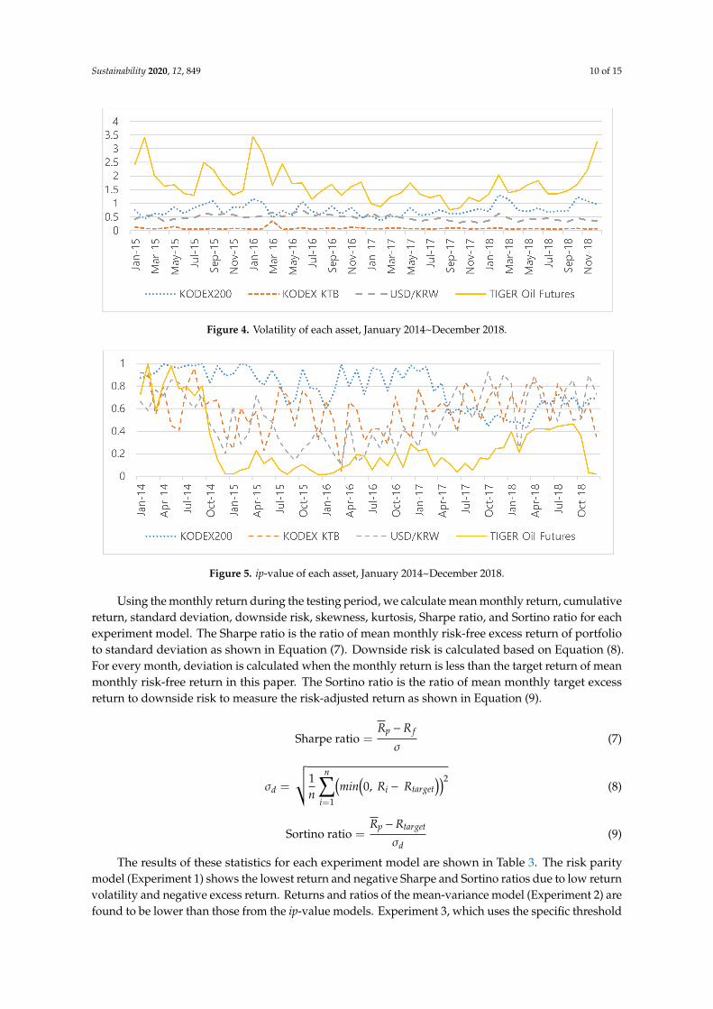
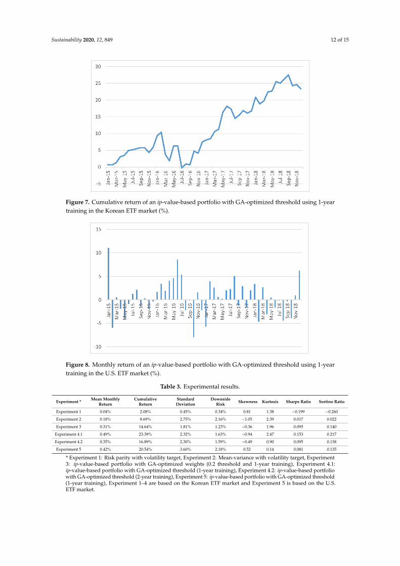
First, the volatility and the ip-value of each ETF are obtained as shown in Figures 4 and 5,respectively. The lower the ip-value is, the higher the instability. When the ip-values in Figure 5are compared with the volatilities of each asset in Figure 4, it is noted that the larger the volatilityis, the lower the ip-value. In the case of bonds, even though the volatility does not seem to change,the ip-value fluctuates because it is based on the rank of iFMII and reflects a low level of volatility.Therefore, the ip-value shows the level of stability of asset movement.

Sustainability 2020, 12, 849 10 of 15

Figure 4. Volatility of each asset, January 2014~December 2018.

Figure 5. ip-value of each asset, January 2014~December 2018.

Using the monthly return during the testing period, we calculate mean monthly return, cumulativereturn, standard deviation, downside risk, skewness, kurtosis, Sharpe ratio, and Sortino ratio for eachexperiment model. The Sharpe ratio is the ratio of mean monthly risk-free excess return of portfolioto standard deviation as shown in Equation (7). Downside risk is calculated based on Equation (8).For every month, deviation is calculated when the monthly return is less than the target return of meanmonthly risk-free return in this paper. The Sortino ratio is the ratio of mean monthly target excessreturn to downside risk to measure the risk-adjusted return as shown in Equation (9).

Sharpe ratio =Rp −R f

σ(7)

σd =

√√1n

n∑i=1

(min

(0, Ri − Rtarget

))2(8)

Sortino ratio =Rp −Rtarget

σd(9)

The results of these statistics for each experiment model are shown in Table 3. The risk paritymodel (Experiment 1) shows the lowest return and negative Sharpe and Sortino ratios due to low returnvolatility and negative excess return. Returns and ratios of the mean-variance model (Experiment 2) arefound to be lower than those from the ip-value models. Experiment 3, which uses the specific threshold

Sustainability 2020, 12, 849 11 of 15

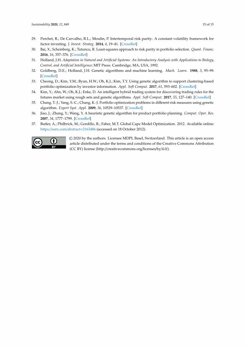
rather than the optimized threshold with 1-year training period, also shows higher returns and ratiosthan those from experiments 1 and 2. Therefore, we can expect that the ip-value-based models bringhigher returns per volatility than the existing models. Additionally, the Sharpe and Sortino ratios ofExperiment 4 are higher than those from experiments 1 and 2. However, we find some differences inresults from the ip-value models using different parameters. The model using a 1-year training period(Experiment 4.1) shows better performance than that using a 2-year learning period (Experiment 4.2).Comparing the results of Experiment 3 and Experiment 4.2, the model using specific threshold and1-year weight optimization by GA shows lower returns but similar Sharpe ratios and higher Sortinoratios. Although assessing the asset allocation model through the returns is important, it is moreimportant to evaluate it through the generated portfolio returns per volatility, which is measured bythe Sharpe and Sortino ratios. From that point of view, 2-year training process may not be appropriatewhen constructing ip-value-based models. Our presented 1-year training model in Experiment 4.1shows the highest mean monthly and cumulative returns as well as the highest Sharpe and Sortinoratios. Therefore, we use the training interval and other parameters of Experiment 4.1 for Experiment5 with U.S. data. We also find that monthly returns from all models except for risk parity model showsleft-tailed distribution with negative skewness and there is no excess kurtosis problem for all models.

Figures 6 and 7 show the monthly return and cumulative return of Korean ETFs over the sampleperiod generated from the ip-value model with a 1-year learning period, respectively. As shown inFigure 6, the portfolio generates mostly positive returns except for several months. In this empiricalanalysis, rebalancing is performed monthly, so there may be some point in time in which asset allocationis not adjusted as sensitively. If the asset allocation is rebalanced on a weekly or daily basis, thisproblem seems to be solved to some extent. Figures 8 and 9 show the monthly return and cumulativereturn of U.S. ETFs over the sample period generated from the ip-value model with a 1-year learningperiod, respectively. As shown in Figure 8, the portfolio generates more frequent positive returns forU.S. ETFs as those for Korean ETFs. We also find that our model generates competitive performance inthe U.S. ETF market as well as the Korean ETF market.

Figure 6. Monthly return of an ip-value-based portfolio with GA-optimized threshold using 1-yeartraining in the Korean ETF market (%).

Sustainability 2020, 12, 849 12 of 15

Figure 7. Cumulative return of an ip-value-based portfolio with GA-optimized threshold using 1-yeartraining in the Korean ETF market (%).

Figure 8. Monthly return of an ip-value-based portfolio with GA-optimized threshold using 1-yeartraining in the U.S. ETF market (%).

Table 3. Experimental results.

Experiment * Mean MonthlyReturn

CumulativeReturn

StandardDeviation

DownsideRisk Skewness Kurtosis Sharpe Ratio Sortino Ratio

Experiment 1 0.04% 2.08% 0.45% 0.34% 0.81 1.38 −0.199 −0.260

Experiment 2 0.18% 8.69% 2.75% 2.16% −1.05 2.39 0.017 0.022

Experiment 3 0.31% 14.64% 1.81% 1.23% −0.36 1.96 0.095 0.140

Experiment 4.1 0.49% 23.39% 2.32% 1.63% −0.94 2.47 0.153 0.217

Experiment 4.2 0.35% 16.89% 2.30% 1.59% −0.49 0.90 0.095 0.138

Experiment 5 0.42% 20.54% 3.60% 2.18% 0.52 0.14 0.081 0.135

* Experiment 1: Risk parity with volatility target, Experiment 2: Mean-variance with volatility target, Experiment3: ip-value-based portfolio with GA-optimized weights (0.2 threshold and 1-year training), Experiment 4.1:ip-value-based portfolio with GA-optimized threshold (1-year training), Experiment 4.2: ip-value-based portfoliowith GA-optimized threshold (2-year training), Experiment 5: ip-value-based portfolio with GA-optimized threshold(1-year training), Experiment 1–4 are based on the Korean ETF market and Experiment 5 is based on the U.S.ETF market.

Sustainability 2020, 12, 849 13 of 15

Figure 9. Cumulative return of an ip-value-based portfolio with GA-optimized threshold using 1-yeartraining in the U.S. ETF market (%).

4. Concluding Remarks

With the emergence of the robo-advisor, the asset allocation model is expected to evolve onestep further. There are few asset allocation models that achieve high diversification effects and reflectthe investment tendency of various investors. A model that can reflect investment tendencies ismore suitable for the future robo-advisor period than the previous risk parity and mean-variancemodels. The model proposed in this paper combines the time series model (or statistical model) tomeasure the degree of instability and GA to optimize the asset weights and thresholds for instability.In this respect, our approach differs from the existing asset allocation models which are based on onlystatistical models. The empirical results show better performance by the proposed model than theprevious models. It is noted that the previous models depend on some assumptions. In contrast, ourmodel does not make any specific assumptions, so it seems more plausible to apply it to actual marketdata. Our model is also used for investors with various investment propensities by using variousthreshold values.

The model proposed in this paper can be used as a portfolio management algorithm or anautomated investment advice to construct a robo-advisor. A procedure to identify investor preferencesshould be added, and then ETFs that match the identified trends can be selected. Furthermore, addinganother component that automatically makes asset trades constructs a robo-advisor. In future research,we plan to assess the proposed model using various ranges of internal parameters for the learningperiod and threshold values.

This study has potential limitations. The model developed in this paper is based on a portfoliothat consists of stocks, bonds, foreign exchange assets, and commodity assets in the Korean ETF market,and U.S. ETF market for model validation. As such, the empirical results are limited to the Koreanand U.S. ETF market data. Based on the idea of our model, a future research can be enriched bydeveloping a model that can be used for other portfolios containing various types of financial assets ina global market.

Author Contributions: Project administrator, K.J.O.; Proposing methodology, programming, formal analysis andwriting—original draft preparation, W.A.; Resources and Data processing, H.R.; Writing—review, editing andvalidation, H.S.L. All authors have read and agreed to the published version of the manuscript.

Funding: This research received no external funding.

Conflicts of Interest: The authors declare no conflict of interest.

Sustainability 2020, 12, 849 14 of 15

References

1. Faloon, M.; Scherer, B. Individualization of Robo-Advice. J. Wealth Manag. 2017, 20, 30–36. [CrossRef]2. Yanagawa, E. Trends and initiatives about robo-advisers: Pioneering unexplored areas in Japan. J. Digit. Bank.

2017, 2, 58–73.3. Poterba, J.M.; Shoven, J.B. Exchange-Traded Funds: A New Investment Option for Taxable Investors.

Am. Econ. Rev. 2002, 92, 422–427. [CrossRef]4. Musto, C.; Semeraro, G.; Lops, P.; De Gemmis, M.; Lekkas, G. Personalized finance advisory through

case-based recommender systems and diversification strategies. Decis. Support Syst. 2015, 77, 100–111.[CrossRef]

5. Lopez, J.C.; Babcic, S.; De La Ossa, A. Advice goes virtual: How new digital investment services are changingthe wealth management landscape. J. Financ. Perspect. 2015, 3, 1–18.

6. Gomes, C.P.; Selman, B. Algorithm portfolios. Artif. Intell. 2001, 126, 43–62. [CrossRef]7. Trippi, R.R.; Turban, E. Neural Networks in Finance and Investing: Using Artificial Intelligence to Improve Real

World Performance; McGraw-Hill, Inc.: New York, NY, USA, 1992.8. Bahrammirzaee, A. A comparative survey of artificial intelligence applications in finance: Artificial neural

networks, expert system and hybrid intelligent systems. Neural Comput. Appl. 2010, 19, 1165–1195. [CrossRef]9. Markowitz, H. Portfolio selection. J. Financ. 1952, 7, 77–91.10. Rubinstein, M.E. A mean-variance synthesis of corporate financial theory. J. Financ. 1973, 28, 167–181.

[CrossRef]11. Li, D.; Ng, W.-L. Optimal Dynamic Portfolio Selection: Multiperiod Mean-Variance Formulation. Math. Financ.

2000, 10, 387–406. [CrossRef]12. Gruber, M.J.; Ross, S.A. The current status of the capital asset pricing model (CAPM). J. Financ. 1978, 33,

885–901. [CrossRef]13. Sharpe, W.F. Capital asset prices: A theory of market equilibrium under conditions of risk. J. Financ. 1964,

19, 425–442.14. Lintner, J. The valuation of risk assets and the selection of risky investments in stock portfolios and

capital budgets. In Stochastic Optimization Models in Finance; Academic Press: Cambridge, MA, USA, 1975;pp. 131–155.

15. Fama, E.F.; French, K.R. The Value Premium and the CAPM. J. Financ. 2006, 61, 2163–2185. [CrossRef]16. Black, F.; Litterman, R. Global Portfolio Optimization. Financ. Anal. J. 1992, 48, 28–43. [CrossRef]17. Drobetz, W. How to avoid the pitfalls in portfolio optimization? Putting the Black-Litterman approach at

work. Financ. Mark. Portf. Manag. 2001, 15, 59–75. [CrossRef]18. Chaves, D.; Hsu, J.; Li, F.; Shakernia, O. Risk Parity Portfolio vs. Other Asset Allocation Heuristic Portfolios.

J. Invest. 2011, 20, 108–118. [CrossRef]19. Anderson, R.M.; Bianchi, S.W.; Goldberg, L.R. Will my risk parity strategy outperform? Financ. Anal. J. 2012,

68, 75–93. [CrossRef]20. Clarke, R.; De Silva, H.; Thorley, S. Risk parity, maximum diversification, and minimum variance: An analytic

perspective. J. Portf. Manag. 2013, 39, 39–53. [CrossRef]21. Roncalli, T.; Weisang, G. Risk parity portfolios with risk factors. Quant. Financ. 2016, 16, 377–388. [CrossRef]22. Kim, D.H.; Lee, S.J.; Oh, K.J.; Kim, T.Y. An early warning system for financial crisis using a stock market

instability index. Expert Syst. 2009, 26, 260–273. [CrossRef]23. Oh, K.J.; Kim, T.Y.; Kim, C. An early warning system for detection of financial crisis using financial market

volatility. Expert Syst. 2006, 23, 83–98. [CrossRef]24. Kim, Y.M.; Han, S.K.; Kim, T.Y.; Oh, K.J.; Luo, Z.; Kim, C. Intelligent stock market instability index:

Application to the Korean stock market. Intell. Data Anal. 2015, 19, 879–895. [CrossRef]25. Qian, E. Risk parity and diversification. J. Invest. 2011, 20, 119. [CrossRef]26. Lohre, H.; Opfer, H.; Ország, G. Diversifying risk parity. J. Risk 2014, 16, 53–79. [CrossRef]27. Benson, R.; Furbush, T.; Goolgasian, C. Targeting Volatility: A Tail Risk Solution When Investors Behave

Badly. J. Index Invest. 2014, 4, 88–101. [CrossRef]28. Hocquard, A.; Ng, S.; Papageorgiou, N. A constant-volatility framework for managing tail risk. J. Portf. Manag.

2013, 39, 28–40. [CrossRef]

Sustainability 2020, 12, 849 15 of 15

29. Perchet, R.; De Carvalho, R.L.; Moulin, P. Intertemporal risk parity: A constant volatility framework forfactor investing. J. Invest. Strateg. 2014, 4, 19–41. [CrossRef]

30. Bai, X.; Scheinberg, K.; Tutuncu, R. Least-squares approach to risk parity in portfolio selection. Quant. Financ.2016, 16, 357–376. [CrossRef]

31. Holland, J.H. Adaptation in Natural and Artificial Systems: An Introductory Analysis with Applications to Biology,Control, and Artificial Intelligence; MIT Press: Cambridge, MA, USA, 1992.

32. Goldberg, D.E.; Holland, J.H. Genetic algorithms and machine learning. Mach. Learn. 1988, 3, 95–99.[CrossRef]

33. Cheong, D.; Kim, Y.M.; Byun, H.W.; Oh, K.J.; Kim, T.Y. Using genetic algorithm to support clustering-basedportfolio optimization by investor information. Appl. Soft Comput. 2017, 61, 593–602. [CrossRef]

34. Kim, Y.; Ahn, W.; Oh, K.J.; Enke, D. An intelligent hybrid trading system for discovering trading rules for thefutures market using rough sets and genetic algorithms. Appl. Soft Comput. 2017, 55, 127–140. [CrossRef]

35. Chang, T.-J.; Yang, S.-C.; Chang, K.-J. Portfolio optimization problems in different risk measures using geneticalgorithm. Expert Syst. Appl. 2009, 36, 10529–10537. [CrossRef]

36. Jiao, J.; Zhang, Y.; Wang, Y. A heuristic genetic algorithm for product portfolio planning. Comput. Oper. Res.2007, 34, 1777–1799. [CrossRef]

37. Butler, A.; Philbrick, M.; Gordillo, R.; Faber, M.T. Global Cape Model Optimization. 2012. Available online:https://ssrn.com/abstract=2163486 (accessed on 18 October 2012).

© 2020 by the authors. Licensee MDPI, Basel, Switzerland. This article is an open accessarticle distributed under the terms and conditions of the Creative Commons Attribution(CC BY) license (http://creativecommons.org/licenses/by/4.0/).