assessment of urans and des for …turbo.mech.iwate-u.ac.jp/fel/papers/gt2010-22325.pdf · the des...

1 Copyright © 2008 by ASME

Proceedings of GT2010 ASME Turbo Expo 2010: Power for Land, Sea and Air

June 14-18, 2010, Glasgow, UK

GT2010-22325

ASSESSMENT OF URANS AND DES FOR PREDICTION OF LEADING EDGE FILM COOLING

Toshihiko Takahashi a , Ken-ich Funazaki b, Hamidon Bin Salleh b, Eiji Sakai c and Kazunori Watanabe c

a Central Research Institute of Electric Power Industry, JAPAN, visiting at the von Karman Institute for Fluid Dynamics b Department of Mechanical Engineering, Iwate University, JAPAN c Central Research Institute of Electric Power Industry, JAPAN

E-mail: [email protected] ( [email protected] ; until Oct. 2010 )

ABSTRACT This paper describes assessment of CFD simulations

for the film-cooling on the blade leading edge with circular cooling holes in order to contribute durability assessment of the turbine blades. Unsteady RANS (URANS) applying a k - ε - v2

- f turbulence model and the Spallart and Allmaras turbulence model, and Detached-Eddy Simulation (DES) based on the Spallart and Allmaras turbulence model are addressed to solve thermal convection. The CFD calculations were conducted by simulating a semi-circular model in the wind tunnel experiments.

The DES and also the k - ε - v2 - f model evaluate explicitly unsteady fluctuation of local temperature by the vortex structures, so that the predicted film cooling effectiveness comparatively in agreement with measurements. On the other hand, the predicted temperature fields by the Spallart and Allmaras model are less diffusive than the DES and the k - ε - v2 - f model. In the present turbulence modeling, the DES only predicts penetration of main flow into the film cooling hole, but the Spallart and Allmaras model is not able to evaluate the unsteadiness and the vortex structures clearly, and over-predict film cooling effectiveness on the partial surface.

INTRODUCTION Application of film cooling technology to gas turbines

progresses in combined power generation plants increasing thermal efficiency with rise in turbine inlet gas temperature. In order to assess durability of the gas turbine blades, it is essential to estimate the temperature distributions of the blades. Accordingly, prediction of film cooling by CFD is important for assessment of the durability. It is necessary for the durability assessment to estimate the cooling performance especially on the leading edge region where flow impinges and heavy thermal load appears. Hence the present study focuses on the CFD prediction of the leading edge film cooling performance.

Experimental investigations of the leading edge film cooling have been previously done and clarified a lot of

important characteristics of the performances. Mick and Mayle [1] had measured film cooling effectiveness and heat transfer on the semi-circular leading edge with three rows of cooling holes. They presents the effectiveness is decreased as the blowing ratio is increased. Mehendale and Han [2] studied the influences of the blowing ratio and the inlet turbulence intensity by using the same model as the Mick and Mayle [1]. Furthermore, Ou, et al.[3], Ekkad, et al. [4] and Johnston, et. al. [5] investigated the influences of inlet turbulence on the cooling performance. Funazaki, et al.[6] studied influences of the incoming periodic turbulence by wakes on the film cooling of the semi-circular leading edge model. Cruse et al. [7] studied the effect of leading-edge shapes on the film cooling effectiveness by using an infrared camera with circular and elliptic leading edge geometries. Reiss and Bölcs [8] examined the influence of the cooling hole geometry on film cooling performance. The authors presented fan-shaped holes increased film cooling performance due to reduced tendency of ‘‘lift off’’ at high blowing ratios. Ou and Rivir[9] employed liquid crystal image to measure the film cooling heat transfer. Ahn, et al.[10] measured the effectiveness on a rotating blade leading edge by using pressure sensitive paints. More recently, Liu, et al.[11] conducted detailed investigation of the hole angle and shape effects by using transient infrared thermography techniques. Falcoz, et al.[12] presents detailed measurements of the film cooling effectiveness with thermochromatic liquid crystal.

With regard to the numerical approaches for film cooling, starting with flat plate configurations, a number of the investigations (ex. [13]-[24] for flat plate configurations, [25]-[36] for leading edge configurations) have been conducted in order to predict the cooling performance and to clarify the physics of the thermal flow field, so far. In terms of the leading edge film cooling, the CFD studies also presented useful knowledge. The United Technology Pratt and Whitney organized the blind test of film cooling calculation on a cylindrical leading edge experiments by Cruse et al. [7]. On this blind test, Lin et al.[25], Martin and Thole [26], Thakur et al.[27] calculated the same thermo-flow field by applying

mailto:[email protected]�

mailto:[email protected]�


different mesh types with discretization schemes and turbulence modeling including a k - ω model and a k - ε model with wall functions. Chernobrovkin and Lakshminarayana [28] also ran simulations for the same flow by a low Reynolds number k - ε model, later. All those computations correctly predicted the tendencies of lateral-averaged effectiveness, but included discrepancies in local effectiveness. Lin et al.[25] and their extended work (Lin and Shih [29]) with the SST model clarified how hot spots can form on the stagnation region due to flow induced by coolant jets. On the other hand, they also indicated that the simulations under-predicted the spread of the coolant in the wall-normal direction. York and Leylek [30], [31] and [32] applied the realizable k - ε turbulence model into the leading edge film cooling in order to investigate the film cooling effectiveness, heat transfer coefficient and the effects of hole shapes, respectively. The authors showed the predictions are generally in good agreement with the experiments, but discrepancies increases with the blowing ratio. All the numerical studies for the leading edge cooling mentioned above had been conducted based on the steady RANS modeling. Those outcomes demonstrate that CFD is able to serve useful information for estimation of the leading edge film cooling.

However, it is fundamentally difficult in principle for the eddy viscosity models in the steady RANS simulations to correctly resolve anisotropic behavior induced by large scale structures which probably are the primal mechanisms of the mixing of the film coolant with the free stream. A Large-Eddy Simulation (LES) and of course DNS are essential to finely resolve turbulence scales. Due to this, the LES has been applied to the calculation of the film cooling; Tyagi and Acharya [23], Guo, et al.[24] for the flat plate configuration, Rozati and Tafti [21], [22] and Sreedharan and Tafti [36] for the leading edge configuration. Those studies have clarified the detailed physics of the film cooling flow. On the other hands, it is supposed to be difficult for the near future environment of high-performance computing, at least for industrial simulations, to estimate the convective heat transfer of cooled blades in a hot section (ex. HPT blades) by the LES. Those convective heat transfer calculations need considerably fine mesh similar to the DNS to resolve turbulence scales to be fine close to the near-wall region. High speed computing and massive resources required make it difficult to apply the full LES to real configurations and conditions of actual cooled blades.

On the above background, this study investigates performances of unsteady CFD calculations by applying RANS modeling to the leading edge film cooling. Taking practicable simulations for industrial problems in the near future into consideration, calculations of unsteady RANS (URANS) and a Detached-Eddy Simulation (DES) are conducted from a view of time-averaged estimation of the cooling performance which is first important for the durability assessment of the cooled blade with large matrix of parameters. The URANS employing the k - ε - v2 - f turbulence model [37],[38] and the Spallart and Allmaras turbulence model [39], and the DES [40], which is

a LES with the Spallart and Allmaras turbulence model in the near-wall region, are addressed to solve thermal convection. In the unsteady calculations, RANS modeling was possibly expected to work as a filter to extract structures having impacts on the cooling performance. The present authors previously calculated the film cooling mainly for flat plate configurations with steady modeling using the k - ω type turbulence model (chiefly by the SST model) and the DES (Sakai, et al.[33]). The authors presented that the DES could predict secondary vortices counter-rotating against the primary vortex pair in the flat plate cooling, which is supposed to enhance lateral spreading of the film coolant. The authors also tried to calculate the leading edge film cooling in addition, but acquired little information for the CFD capability for the leading edge film cooling. The present calculations were conducted by simulating an experiment of the semi-circular leading edge model. Distributions of film cooling effectiveness on the model surface and temperatures distributions in the flow field are compared with the measurements with a thermo-probe consisting of thermocouples and thermochromatic liquid crystal. Thermo-flow characteristics predicted by the present unsteady calculations were investigated.

NOMENCLATURE BR : Blowing ratio, ρ2 U2 / ρm Um ,

l f ll li h l D : Diameter of the leading edge model, m d : Diameter of film cooling holes, m h : Heat transfer coefficient, W/(m2K)

LQ : Thermochromatic liquid crystal n : Wall-normal distance, m Q : Second invariant of gradient of velocity tensor q : Heat flux, W/m2

ReD : Reynolds number , ρUm D/µ T : Temperature, K

TC : Thermocouples t : Time, s U : Mean velocity, m/s

x, y, z : Cartesian coordinates, m α : Angle, deg. η : Film cooling effectiveness, ( Tm - Taw )/(Tm – T2 ) µ : Viscosity, Pa s ρ : Density, kg/m3

Subscripts aw : Adiabatic wall ave : Average in the pitch-wise direction of the model

Hole : Relative to each cooling hole m : Relative to main flow w : Wall 2 : Relative to film flow


LEADING EDGE MODEL Fig. 1 shows the leading edge model used in the numerical

calculations and experimental measurements. The leading edge model consists of a semi-circular geometry of 80 mm diameter and a flat after-body. The model has plenum inside to supply the secondary air as film coolant through film cooling holes. On the wall of the model, the film cooling holes of 8 mm diameter are periodically placed with staggered arrangement in the three rows. Hole angle is 30 degrees to the model surface in the height-wise direction, and the pitch of the periodic holes is 62 mm (7.72d). Two rows of the film cooling holes, Hole1 (Row1) and Hole2 (Row2), are located at 15 degrees on both side from the stagnation line in case without film cooling. The other row of the film cooling hole, Hole3 (Row3), is placed at 50 degrees from the stagnation. As shown in Fig.2 (a), the computational domain simulating the experimental setups is composed of the primary domain, the secondary chamber, and the connecting duct between the primary domain and the chamber. The primary domain is a pitch of the periodical arrangement of the film cooling holes in the height-wise direction, consisting of the main stream region, the film cooling holes (Hole1, Hole2, and Hole3), and the plenum as shown in Fig.2(b).

DESCRIPTIONS OF NUMERICAL CALCULATIONS The “FLUENT” code based on the finite volume method

was used in the numerical calculations. Unsteady Reynolds-averaged and filtered Navier-Stokes equations were solved with the URANS models and the DES, respectively. The discretized equations are solved by the SIMPLE algorithm (Patanker and Spalding [41]) with time integration. The second order implicit scheme is utilized for the time integral of both the URANS and the DES with a non-dimensional time step of 4.05 x 10-4 D/Um. Time-averaged statistics were accumulated over the period of about 8D/ Um. URANS

Unsteady Reynolds-averaged Navier-Stokes equations were solved with k - ε - v2 - f model [37], [38] (V2F) and the Spallart and Allmaras model [39] (SA). The V2F was employed to attempt to correctly treat wall asymptotic behaviors of the turbulent properties and to avoid production of anomalous turbulent energy in the flow around the leading edge by a two-equation eddy viscosity model. Regarding this point for the SA, the turbulence production is evaluated based on the antisymmetric components of the velocity gradient tensor (the vorticity tensor). The convective terms of the momentum equations were discretized by the third order MUSCL scheme [42] and the other terms are solved with the second order central difference scheme.

DES

The DES modeling [40] based on the Spalart-Allmaras model [39] was applied. The DES model replaces the length

scale dw in the SA, which is the distance to the closest wall, with the length scale defined as;

l = min(dw, Cdes Δ) (1)

where Δ is based on the largest grid space in the x, y, or z

Fig.2 Computational domain (b) Primary domain (extracted from the whole domain)

(a) Whole domain

Fig.1 Leading edge model


directions forming the computational cell, and Cdes (=0.65) is the empirical constant. The second order central difference scheme is applied into all the spatial discretizations of the momentum equations. Computational mesh and conditions

Fig.3 shows outline of the computational mesh (surface mesh) employed in the calculations. Unstructured grid system which consists of hexahedral cells and tetra cells was employed to solve the discretized equations. Except in the plenum and the secondary air chamber, the hexahedral cells are generated in the main stream region and the film cooling holes.

It supposed to be some challenge to search grid convergence for the DES switching the modeling from the LES to the SA close to the wall as indicated by the eq.(1). In the present, however, just focused on the leading edge portion with a very thin boundary layer in the whole domain, near wall mesh is fined by using hanging nodes in order to secure resolution. Total number of the cells is 3,995,322; 1,898,260 cells in the main stream region around the leading edge model, 1,783,376 cells in the film cooling holes, 271,830 cells in the plenum, and 41,856 cells in the secondary air chamber. The cells on the model surface are formed layered-structure in the near wall regions. The value of y+ for the computational point of the first cell above the wall is less than unity so that the wall function approach is not applied on the wall. For a reference of mesh dependency in the solutions, Fig.4 shows comparisons of span-wise averaged film cooling effectiveness on the model between the DES calculations with the primary mesh mentioned above and a coarse mesh. The computational conditions are shown later. The total cell number of the coarse mesh is 1,422,738; 587,748 cells in the main stream region, 521,304 cells in the film cooling holes, 313,686 cells in the other regions. The coarse mesh results show only a small difference from the primary mesh ones. In the present study, the primary mesh had been employed for all the calculations of the DES and URANS.

Table 1 shows inlet conditions for the numerical calculations. In this study, the temperature of the secondly air was set at higher than the main flow temperature, according as experimental conditions as presented below. All the calculations were performed for Reynolds number ReD of 8.55 x 104, based on the model diameter D and inlet flow conditions. Two cases for the mean blowing ratio (BR~1, 2) of the three holes Hole1, Hole2 and Hole3 are calculated for each of the turbulence model. Adiabatic conditions were imposed on the wall of the model. Mass flow rate, total temperature and turbulent quantities were imposed at the inlets of the main stream region and the secondary air chamber, and the static pressure is set at both the outlets of the main stream region and the plenum. The static pressure at the plenum outlet was specified to balance a mean mass flow in film cooling holes which is determined by the prescribed mean blowing ratio BR. With regard to the inlet turbulence quantities in the each turbulence model, steady component is set at constant on the

basis of the turbulence intensity of 0.1%, referred to the wind tunnel experiment. Unsteady components of the flow primitives are not given at the inlets in the calculations.

All the computations were executed with a PC cluster of eight CPUs. The process time per CPU for the DES and the SA is approximately five seconds per iteration in the SIMPLE algorithm, and the process for the V2F took about 20% longer than for the SA, because of the number of the equations.

Fig.3 Outlines of CFD mesh (Surface mesh) (b) Mesh around leading edge (expanded)

(a) Mesh of the primary domain

Fig.4 Variations of predicted effectiveness with mesh

ηav

e

DES Primary mesh BR= 1.03DES Coarse mesh 1.02Experiment, LQ 1.06

s/d

deg.α-90 -60 -30 0 30 60 900

0.1

0.2

0.3

0.4

0.5-15 -10 -5 0 5 10 15


Table 1 Computational conditions

ρmUm ,

kg/(m2s) Tm, K ρ2U2 ,

kg/(m2s) T2, K 2nd air chamber

supply, kg/s

BR ~ 1 19.29 291.17 19.82(DES) 19.87(V2F) 20.06(SA)

321.15 0.030

BR ~ 2 19.28 290.57 41.06(DES) 41.60(V2F) 41.85(SA)

329.15 0.030

Table 2 Experimental conditions (a) Measurements with thermocouples (TC)

ρmUm ,



supply, kg/s

BR ~ 1 19.87 291.17 21.06 340.15 0.038

BR ~ 2 19.75 290.57 40.29 345.15 0.041

(b) Measurements with thermochromatic liquid crystal(LQ)

ρmUm ,



supply, kg/s

BR ~ 1 20.10 292.75 21.30 318.15 0.036

BR ~ 2 20.15 291.45 41.10 327.15 0.042

EXPERIMENTENTAL MEASUREMENTS Local temperatures on and around the leading edge

model, which is installed in a test section of a low speed wind tunnel, were measured with thermocouples and thermochromatic liquid crystal applied on the model surface. Turbulence intensity of the main stream into the test section of the wind tunnel is less than 0.5%.

Locations of the temperature measurement by the thermocouples are shown in Fig.5 in red. The temperature distributions on four traverse planes normal to the model surface, shown in Fig.5 (a), were measured by a probe of a K-type thermocouple. On each of the plane of 5d x 7.72d (a pitch of the periodic hole arrangement), temperatures are measured on 17 x 9 crossing points of the grid lines shown in the Fig.5 (b) by traversing the probe. Local temperature profile of very near wall fields is also measured on the half surface of the model at the same side as the above flow field measurements, as a surface temperature by using the thermocouple probe. Wall temperature profile on the whole surface of the model was also measured by the transient method using thermochromatic liquid crystal with two video cameras set at each side of the model, which is referred in Sakai, et al.[33]. Those temperatures measured were converted to film cooling effectiveness. The experimental details were described in Takahashi, et al[43], Sakai, et al. [44] and Funazaki and Binsalleh[45] including information for uncertainties in the measurement of the thermochromatic liquid crystal. Table 2 presents the experimental condition for each of the measurement.

RESULTS AND DISCUSSION Blowing ratio of each film cooling hole

Fig. 6 shows time-averaged fraction of blowing ratio for each film cooling hole to the mean blowing ratio BR for the three holes. All the turbulence models estimate nearly the same blowing ratio fractions for each of the cooling hole. The blowing ratio of the Hole1 and Hole2 where are located close to the stagnation region are smaller than the Hole3. In case of the small mean blowing ratio (BR ~ 1), the blowing ratio fraction of the Hole2, as which the Hole3 is located in the same side of the semi-circular model, is larger than the Hole1 located on the opposite side at the same angle form the stagnation line without film holes as the Hole2. Those differences of the blowing ratio fractions are due to static pressure distribution around the leading edge model, and decreases with increase of the mean blowing ratio BR, because of the increase of the dynamic pressure of the secondary flow ejecting. Hereinafter, the mean blowing ratio BR is designated as a “blowing ratio”.

(a) Measured planes (b)Measurement points in each plane

Fig.5 Locations of temperature measurement by TC

Hole1 Hole2 Hole3

BR

BRH

ole /

BR

DESV2FS A

1 2

0.8

1

1.2

Fig.6 Fraction of blowing ratio for each cooling hole

- 30° 5d

α= - 90°

- 70°

- 40°

7.75d

Measurement pitch: 1mm, 2mm, 5mm

Main flow

Row3

Row2 Row1

Model surface


Film cooling effectiveness on the model surface

Fig. 7 shows predicted distributions of time-averaged local film cooling effectiveness on the model surface. And Fig.8 (a) and (b) show measured distributions of the film cooling effectiveness with thermocouple probe (a) and the thermochromatic liquid crystal (b), respectively. The black area in the Fig.8 (b) is owing to no reaction of the thermochromatic liquid crystal in the transient method. The measured distribution agrees with each other for the angle α < 0º, and the

numerical distributions and their variations with the blowing ratio BR are generally similar as the experimental measurements. Both of the measurements and the predictions indicate that local effectiveness decreases and film coverage get worse with increase of the blowing ratio BR, owing to increase of penetration of the ejected secondary air into main flow. All the results also show that the film coverage region leans downward of the model as the blowing ratio BR increases.

(a) DES (b) V2F (c) SA Fig.7 Time-averaged local adiabatic effectiveness

η

BR=1.03

BR=2.13

BR=1.03

BR=2.16

BR=1.04

BR=2.17

6.0

4.0

2.0

0.0

6.0

4.0

2.0

0.0 -90 0 90

α deg. -90 0 90

α deg. -90 0 90

α deg.

Hole3

Hole2

Hole1 Hole3

Hole2

Hole1 Hole3

Hole2

Hole1

Hole3

Hole2

Hole1 Hole3

Hole2

Hole1 Hole3

Hole2

Hole1

(b) Measurements with thermochromatic liquid crystal (LQ) (Black area is due to no reaction of liquid crystal)

90 20 α deg. -20 -90 α deg.

6.0

4.0

2.0

0.0

90 20 α deg. -20 -90 α deg.

6.0

4.0

2.0

0.0

BR=1.06

BR=2.04

HOLE3

HOLE2

HOLE1

HOLE3

HOLE2

HOLE1

BR=1.06

BR=2.04

(a) Measurements with thermocouples(TC)

Fig.8 Measured distributions of adiabatic effectiveness

η

1.0

0.0

-20 -90 α deg.

BR=1.09

HOLE3

HOLE2

6.0

4.0

2.0

0.0

-20 -90 α deg.

BR=1.89

HOLE3

HOLE2

6.0

4.0

2.0

0.0


The CFD calculations, however, predict local higher

effectiveness than the measurements in regions downstream of the trailing edges of the film cooling holes, as shown in the Fig.7. This local high effectiveness in the prediction is more remarkable and concentrated spatially in the predictions by the SA than in the other predictions, especially as shown in the region downstream of the Hole3. Furthermore, the distribution by the SA in the case of the smaller blowing ratio (BR =1.04) shows a peak area (a plateau) of high effectiveness down the Hole1 (α >30º), which is not found in the experimental measurement by the thermochromatic liquid crystal of the Fig.8 (b) (BR =1.06) and in other numerical predictions.

Fig. 9 shows time-averaged distributions of the span-wise averaged film cooling effectiveness. In these figures, previous results by steady calculations using the SST model (Sakai, et al. [33]) are also included. The figures indicate that all the CFD calculations have reasonable capabilities to predict the spatial averaged profiles of the leading edge film cooling. The DES and the V2F results are comparatively in agreement with the measurements. But, the SA of BR =1.04 as shown in the Fig.7 and also the previous steady calculation by the SST model of BR =2.05 predict the high effectiveness in the downstream region of the Hole1 (α >30º), which appear to be qualitatively different from the measurement.

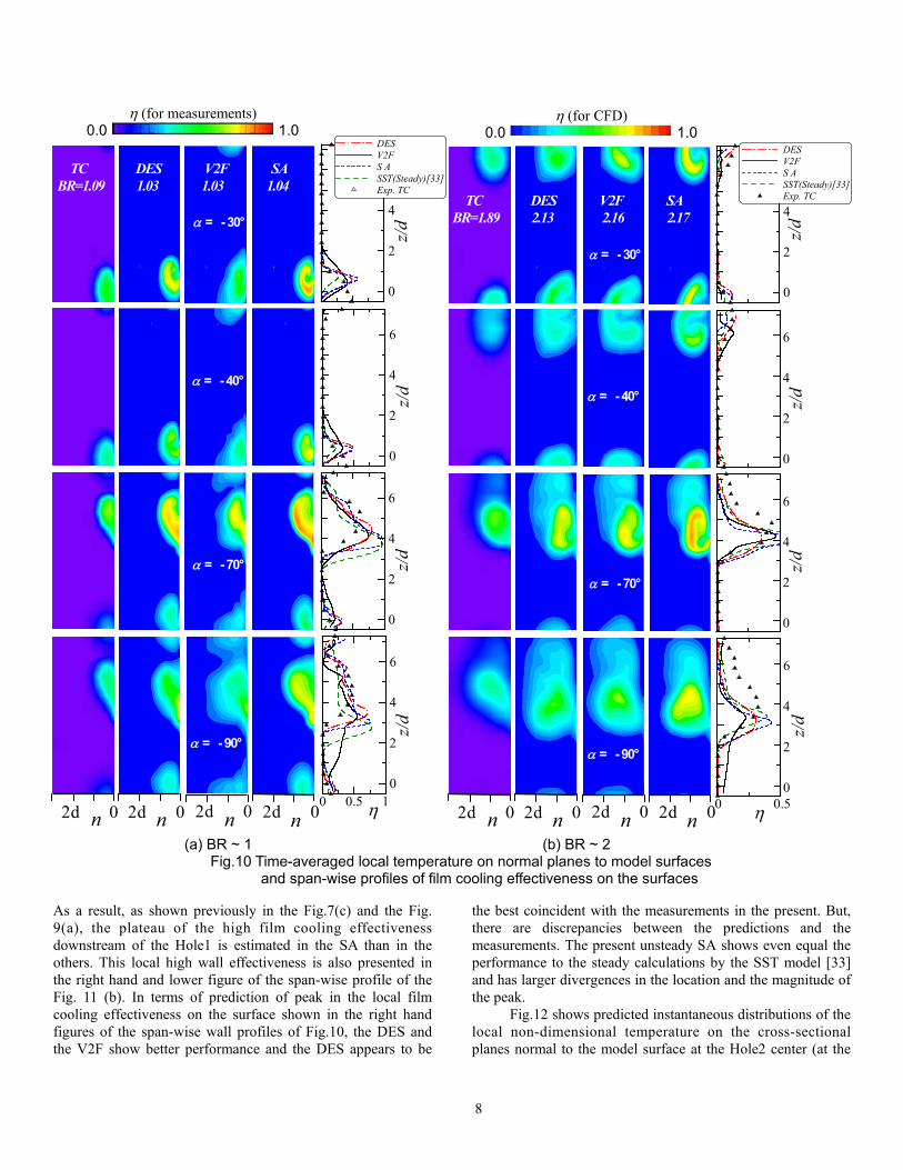
Local temperature distribution around the model Fig.10 shows time-averaged distributions of measured

and predicted local temperature on transverse planes normal to the model surface, at each angle of α = -30º, -40º, -70º and -90º, where is downstream of the Hole2 and the Hole3. In the Fig.10, time-averaged span-wise profiles of the local film cooling effectiveness on the model surface are also presented at the same angles α as those normal planes in the flow field. The CFD results shown in these figures are time-averaged, and the measurement data are acquired by traversing the thermocouples. The local temperature on the normal plane is non-dimensionalized by the same definition as the film cooling effectiveness η. The previous steady calculations using the SST model (Sakai, et al. [33]) are also included in the figures of the span-wise profiles on the model surface.

Every turbulence model shows relatively good performance for predicting location of bulk of the secondary air ejected into the main flow on the normal planes, and simulates departures of the secondary air from the surface with increase of the blowing ratio BR. The V2F, especially as shown in the Fig.10 (b) in case of BR~1, appears to have advantage in the prediction of the location of the bulk secondary air on the normal plane. Distributed patterns of the local temperature supposed to be affected by a so-called kidney-shape vortex pairs, which are found clearly in the results by the SA at the angles α = -30° of BR=1.04 and α = -30°, -40° of BR=2.17. Those predicted patterns of the local temperature indicate that the vortices like the kidney-shape does not have a symmetric structure with respect to the center of the cooling holes as found in the flat plate cooling. In this leading edge film cooling, the entrainment of the main flow by the vortex appears to be larger on the upper side (the leading edge side of the hole) than on the lower side (on the trailing edge side of the hole), so that the film cooling effectiveness is higher on the trailing edge side of the hole as shown in Fig.7.

Regarding those structures on the local temperature in the flow field, all the CFD calculations predict similar aspects, but the SA estimates higher non-dimensional temperature in their core regions than the V2F and the DES. These local distributions predicted by the V2F and the DES appear to be more diffusive and are consistent with aspects in the measurements. And as shown in the Fig.10 (b) of the higher blowing ratio (BR~2), the V2F and the DES estimate the same extent of the normal spreading of the secondary air as the measurements, but the SA under-estimates that. In the Fig. 10 (a) of the lower blowing ratio (BR~1), the normal spreading predicted by the V2F is a little larger than by the DES, but the spreading of the secondary air in every calculation shows the similar extent each other. Furthermore, in the Fig.11 presenting the predicted time-averaged local temperature distributions on normal planes to the model surface downstream of the Hole1 (at angles α = 30º, 60º), The SA evaluates the bulk of the secondary air remarkably to be closer to the wall, shown in Fig.11 (a) of BR=1.04. And the normal spreading of the secondary air in the SA is also smaller than the other models.

ηav

e

Exp., TC, BR= 1.89 LC, 2.04DES 2.13V2F 2.16SA 2.17SST(Steady)[33] 2.05

deg.α

s/d

-90 -60 -30 0 30 60 900

0.1

0.2

0.3

0.4

0.5-15 -10 -5 0 5 10 15

(b) BR ~2

Fig.9 Time-averaged distributions of span-wise averaged film cooling effectiveness

ηav

e

Exp., TC, BR= 1.09 LC, 1.06DES 1.03V2F 1.03SA 1.04SST(Steady)[33] 1.00

s/d

α deg.-90 -60 -30 0 30 60 900

0.1

0.2

0.3

0.4

0.5-15 -10 -5 0 5 10 15

(a) BR ~1


As a result, as shown previously in the Fig.7(c) and the Fig. 9(a), the plateau of the high film cooling effectiveness downstream of the Hole1 is estimated in the SA than in the others. This local high wall effectiveness is also presented in the right hand and lower figure of the span-wise profile of the Fig. 11 (b). In terms of prediction of peak in the local film cooling effectiveness on the surface shown in the right hand figures of the span-wise wall profiles of Fig.10, the DES and the V2F show better performance and the DES appears to be

the best coincident with the measurements in the present. But, there are discrepancies between the predictions and the measurements. The present unsteady SA shows even equal the performance to the steady calculations by the SST model [33] and has larger divergences in the location and the magnitude of the peak.

Fig.12 shows predicted instantaneous distributions of the local non-dimensional temperature on the cross-sectional planes normal to the model surface at the Hole2 center (at the

(a) BR ~ 1 (b) BR ~ 2 Fig.10 Time-averaged local temperature on normal planes to model surfaces

and span-wise profiles of film cooling effectiveness on the surfaces

α = - 30°

α = - 40°

α = - 70°

α = - 90°

2d 0 n

n

n

n

2d 0

2d 0

2d 0

TC DES V2F SA BR=1.09 1.03 1.03 1.04

DESV2FS ASST(Steady)[33]Exp. TC

z/d

0

2

4

η

z/d

0 0.5 10

2

4

6

z/d

0

2

4

6

z/d

0

2

4

6

α = - 30°

α = - 40°

α = - 70°

α = - 90°

2d 0 n

n

n

n

2d 0

2d 0

2d 0

TC DES V2F SA BR=1.89 2.13 2.16 2.17

DESV2FS ASST(Steady)[33]Exp. TC

z/d

0

2

4

z/d

0

2

4

6

ηz/

d0 0.5

0

2

4

6

z/d

0

2

4

6

η (for measurements) 0.0 1.0

η (for CFD) 0.0 1.0


angle α = - 15º) of BR~1. In the present turbulence models, the DES predicts the smallest scales around the interface between the main flow and the secondary air. The V2F also shows the wave pattern around there, but in the SA, the interface has no fluctuation found. Here, the DES only could predict instantaneous penetration of the main flow into the film hole. That is useful for the assessment of the blade durability on the safe side.

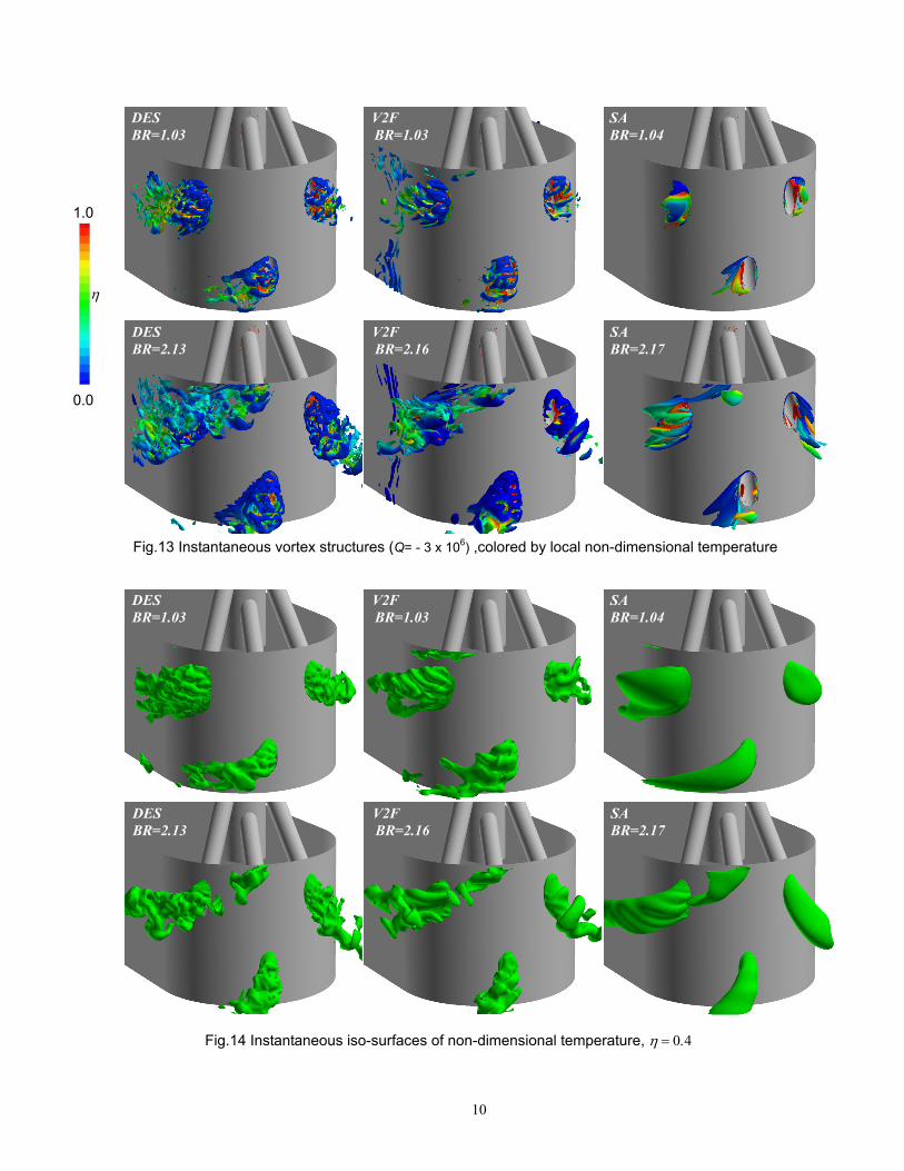
Thermo-flow structures

Fig.13 presents predicted instantaneous views of vortex structures, colored by the local non-dimensional temperature. These vortex structures are represented by iso-surfaces of second invariant of gradient of velocity tensor Q. The non-dimensional temperature is evaluated by the same definition as the film cooling effectiveness η.

The predictable flow scales depend upon the turbulence model, and there are large differences between the SA and the others. Those result from differences in estimations of the eddy viscosity among the turbulence models. The DES and The V2F predict vortex structures representing anisotropic motions, and the DES presents smaller scales resolved than the V2F. The extracted vortex structures from the DES results are found in slightly longer areas downstream of the holes than the V2F results. To the contrary, the SA evaluates the markedly short area where the vortices are found downstream of the holes. Those aspects indicate that the predicted flows by the DES and the V2F promote mixing by the vortex structures more than the flow predicted by the SA.

What the “Reynolds averaging” in the unsteady problem actually represents does not suppose to be well known. In this study, however, both the V2F and the SA based “Reynolds averaging” are conducted with the same mesh resolution and the same temporal integration as the DES. It is important at least that those discretized equations appropriately evaluate the eddy viscosity at each cell and each time step. The present

(a) BR ~ 1 (b) BR ~ 2 Fig.11 Time-averaged local temperature on normal planes to model surfaces

and span-wise profiles of film cooling effectiveness on the surfaces

Fig.12 Instantaneous local temperature on normal planes to the surface, BR~1

η 0.0 1.0

Penetration of main flow

DES V2F SA BR=1.03 1.03 1.04

Hole2 Hole2 Hole2

η 0.0 1.0

η

z/d

0 0.5 10

2

4

6

DESV2FS A

z/d

0

2

4

2d 0

2d 0

2d 0 n

n

n

α = 30°

α = 60°

DES V2F SA BR=1.03 1.03 1.04

DESV2FS A

z/d

0

2

4

η

z/d

0 0.50

2

4

6

2d 0

2d 0

2d 0 n

n

n

α = 30°

α = 60°

DES V2F SA BR=2.13 2.16 2.17


Fig.13 Instantaneous vortex structures (Q= - 3 x 106) ,colored by local non-dimensional temperature

DES V2F SA BR=1.03 BR=1.03 BR=1.04

DES V2F SA BR=2.13 BR=2.16 BR=2.17

DES V2F SA BR=1.03 BR=1.03 BR=1.04

DES V2F SA BR=2.13 BR=2.16 BR=2.17

Fig.14 Instantaneous iso-surfaces of non-dimensional temperature, η = 0.4

η

1.0 0.0


numerical results show that the SA of the one-equation model which is not able to correctly take the “turbulence length scale” yields a stronger spatial filter than the others. On the other hand, the V2F, which takes into account the wall asymptotic behaviors of the turbulence properties with four constitutive equations, appears to reasonably estimate the eddy viscosity. But in the RANS, especially the V2F, there must be also influences of the MUSCL (up-wind) scheme on the predictions.

The DES and V2F similarly predict distinctive vortex structures at around envelopes of the bulk structures, where are shear-layers between the main flow and the ejected secondary air. Inside these shear-layer vortices in the DES and the V2F, other structures with higher non-dimensional temperature are found. But, in the SA calculations, the shear-layer vortex structures are not found. As shown in predicted instantaneous iso-temperature surfaces (η =0.4) of the Fig.14 (at the same angle of depression as the Fig.13), the DES and also the V2F predict fluctuations of the local temperature. These pictures for the DES and the V2F in the Fig.14 exhibit chiefly that the structures in the shear-layers influence the fluctuations of the local temperature. On the other hands, the SA estimates the

smooth iso-surfaces indicating small fluctuation of the local temperature field. These aspects are consistent with the local temperature distributions on the cross-sectional planes in the flow field, presented in the Fig.12.

Fig.15 views predicted time-averaged (a) and instantaneous (b) iso-temperature surfaces (η =0.4 ) form the bottom of the model for the blowing ratio BR~1. In every instantaneous picture in the Fig.15 (b), the volumes wrapped by the temperature iso-surfaces are seen to remain downstream of the film cooling holes along the surface curvature of the model. The SA only predicts the continuous volumes along the model surface in the instantaneous picture. As shown in the Fig.15 (a) for the time-averaged views, however, the DES and the V2F presents the volumes to be shorter downstream of the holes (clearly for downstream of the Hole1) than the SA. These are supposed to be due to the fact that the DES and also the V2F evaluate the mixing by the unsteady vortex structures. On the contrary, the SA estimates distinctively the long time-averaged volumes of the temperature which are similar to the instantaneous one. Those characteristics of the predicted flow structures different from each turbulence modeling give information for the diffusion behavior of the local temperature field.

The high film cooling effectiveness downstream of the Hole1 (α >30º) at BR=1.04 in the SA, presented before in the Fig.7(c) and the Fig.9 (a), is relevant to the predicted characteristics of the local temperature field mentioned above. It seems that the stable and continuous volume of higher temperature above the surface than the main flow temperature could be brought closer to the surface in the flow accelerated along the curvature of the leading edge as shown in the Fig.11 (a). This disadvantage found in the present unsteady simulation of the SA model would be also true with the steady RANS simulations, as presented in the Fig.9 (c) for the span-wise averaged effectiveness by the SST model. The present results illustrate a risk that the steady simulation which is not able to evaluate unsteady vortices also fails to predict even a spatial-averaged performance of film cooling on a curved surface.

In this regard, however in the present study, the temperature of the secondly air was set at higher than the main flow temperature according to the experimental conditions. Consequently, the opposite influence to the present result would be found in the inherent film cooling.

CONCLUSIONS In order to horizontally assess unsteady CFD calculations

by using RANS modeling for prediction of the film cooling on the semi-circular leading edge model, the URANS simulations employing the k - ε - v2 - f model and the Spallart and Allmaras turbulence model, and the DES based on the Spallart and Allmaras turbulence model were performed and those results were compared with the temperature measurements with the thermocouples and thermochrimatic liquid crystal. As a result, some aspects for the performances of those CFD simulations were brought out in the followings.

Fig.15 Iso-surfaces of non-dimensional temperature, η =0.4, BR~1, views from the bottom of the model

(b) Time-averaged view

DES BR=1.03

Model surface Model surface Model surface Hole1

Hole3

Hole2

Hole1

Hole3

Hole2

Hole1

Hole3

Hole2

V2F BR=1.03

SA BR=1.04

Hole1

Hole3

Hole2

Hole1

Hole3

Hole2

Hole1

Hole3

Hole2

Model surface Model surface Model surface

(a) Instantaneous view

DES BR=1.03

V2F BR=1.03

SA BR=1.04


The DES and the k - ε - v2 - f model presented good performances in estimations of time-averaged, span-wise-averaged film and local cooling effectiveness on the leading edge surface. Overall, it was concluded that the predicted temperature fields by these simulations were more diffusive and comparatively in agreement with the measurements than the Spallart and Allmaras model and the steady calculation by the SST model done previously. However, there were some quantitative discrepancies in the time-averaged local peak of the effectiveness on the surface in the predictions by the DES and the k - ε - v2 - f model. The Spallart and Allmaras model predicted the high film cooling effectiveness on the partial surface at angle α >30º in case of the blowing ratio BR~1, which was not found in the measurement. That was also similar as the steady calculations by the SST model.

The DES and also the k - ε - v2 - f model evaluated explicitly unsteady fluctuation of local temperature induced by the vortex structures (anisotropic motions). However, the Spallart and Allmaras model could not clearly predict the unsteadiness and the anisotropic motions despite of the unsteady simulation. In the present turbulence modeling, the DES resolved the smallest scale, and only predicted penetration of main flow into the film cooling hole. The k - ε - v2 - f model predicted similar structures to the DES, but did not show that penetration of the main flow. Those were due to differences in the evaluations of the eddy viscosity among the models.

The partial over-estimation of the local film cooling effectiveness by the Spallart and Allmaras model mentioned above is supposed to be due to lack of the unsteady vortex structures in the accelerated flow along the leading edge curvature. This disadvantage found in the present unsteady simulation of the Spallart and Allmaras model would be also true with ordinary steady RANS simulations.

REFERENCES [1] Mick, W.J., and Mayle, R.E., 1988, “Stagnation Film Cooling and Heat Transfer including its Effect Within the Hole Pattern,” ASME Journal of Turbomachinery, 110, pp. 66-72. [2] Mehendale, A.B., and Han, J.C., 1992, “Influence of High Mainstream Turbulence on Leading Edge Film Cooling Heat Transfer,” ASME Journal of Turbomachinery, 114, pp. 707-715 [3] Ou, S., Mehendale, A. B., and J.C. Han, J. C., 1992, “Influence of high mainstream turbulence on leading edge film cooling heat transfer: effect of film hole row location,” ASME Journal of Turbomachinery. 114, pp.716–723. [4] Ekkad, S.V., Han, J.C., and Du, H., 1998, “Detailed Film Cooling Measurements on a Cylinder Leading Edge Model: Effect of Free-Stream Turbulence and Coolant Density,” ASME Journal of Turbomachinery, 120, pp. 799-807. [5] Johnston, C.A., Bogard, D.G., and McWaters, M.A., 1999, “Highly Turbulent Mainstream Effects on Film Cooling of a Simulated Airfoil Leading Edge,” ASME Paper 99-GT-261. [6] Funazaki, K, Yokota, M., and Yamawaki, S., 1997, ”effect of Periodic Wake Passing on Film Effectiveness of Discrete

Cooling Holes Around the leading Edge of a Blunt Body,” ASME Journal of Turbomachinery, 119, pp.292-301. [7] Cruse, M.W., Yuki, U.M., and Bogard, D.G., 1997, “Investigation of Various Parametric Influences on Leading Edge Film Cooling”, ASME Paper 97-GT-296 [8] Reiss, H. and Bölcs, A., 2000, “Experimental study of showerhead cooling on a cylinder comparing several configurations using cylindrical and shaped holes,” ASME Journal of Turbomachinery,. 122, pp. 161–169. [9] Ou, S., and Rivir, R.B., 2001, “Leading Edge Film Cooling Heat Transfer with High Free Stream Turbulence Using a Transient Liquid Crystal Image Method,” Int. Journal of Heat and Fluid Flow, 22, pp. 614-623. [10] Ahn, J., Schobeiri, M.T., Han, J. C. and Moon, H. K., 2005, “Film Cooling Effectiveness on the Leading Edge of a Rotating Film-Cooled Blade Using Pressure Sensitive Paint,” GT2005-68344. [11] Lu, Y., Allison, D., and Ekkad, S. V., 2006, “Influence of Hole Angel and Shaping on Leading Edge Showerhead Film Cooling,” GT2006-90370. [12] Falcoz a, C., Weigand, B. and Ott, P., 2006, “Experimental investigations on showerhead cooling on a blunt body,” Int. Journal Heat and Mass Transfer, 49, pp.1287-1298. [13] Walters, D. K. and Leylek, J. H., 1997,“A Systematic computational Methodology Applied to a Three-dimensional Film-cooling Flowfield,” ASME Journal of Turbomachinery, 119, pp.777-785. [14] Walters, D. K. and Leylek, J. H., 2000,“A Detailed Analysis of Film-Cooling Physics: Part I- Streamwise Injection With Cylindrical Holes,” ASME Journal of Turbomachinery, 122, pp.103-112. [15] Hyams, D. G. and Leylek, J. H., 2000,“A Detailed Analysis of Film-Cooling Physics: Part II- Compound-Angle Injection WithCylindrical Holes,” ASME Journal of Turbomachinery, 122, pp.113-121. [16] McGovern, K. T. and Leylek, J. H., 2000,“A Detailed Analysis of Film-Cooling Physics: Part III- Streamwise Injection With Shaped Holes,” ASME Journal of Turbomachinery, 122, pp.122-132. [17] Brittingham, R. A. and Leylek, J. H., 2000,“A Detailed Analysis of Film-Cooling Physics: Part Part IV- Compound-Angle Injection With Shaped Holes, ASME Journal of Turbomachinery, 122, pp.133-145. [18] Hassan, J. S. and Yavuzkurt, S., 2006, “Comparison of Four Different Two-equation Models of Turbulence in Predicting Film Cooling Performance,” GT2006-90860. Na, S., Zhu, B., Bryden, M. and Shih, T. I-P., 2006, “CFD Analysis of Film Cooling,” AIAA 2006-22 [19] Bacci, A. and Facchini, B., 2007, “Turbulence Modeling for the Numerical Simulation of Film and Effusion Cooling Flows,” GT2007-27182. [20] Yavuzkurt, S. and Hassan, J. S., 2007, “ Evaluation of Two-equation Models of Turbulence in Predicting Film Cooling Performance under High Free Stream Turbulence,”


GT2007-27184. [21] Yavuzkurt, S. and Habte, M., 2008, “Effect of Computational Grid on Performance of Two-equation Models of Turbulence for Film Cooling Applications,” GT2008-50153. [22] Harrison, K. L. and Bogard, D. G., 2008, “Comparison of RANS Turbulence Models for Prediction of Film Cooling Performance,” GT2008-51423. [23] Tyagi, M. and Acharya, S., 2003, “Large Eddy Simulation of Film Cooling Flow From an Inclined Cylindrical Jet,” ASME Journal of Turbomachinery, 125, pp. 734-742. [24] Guo, X., Meinke, M., and Schröder, W., 2006, “Large-Eddy Simulation of Film Cooling Flows.” Computers and Fluids, 35(6), pp. 587-606. [25] Lin, Y.-L., Stephens, M. A., and Shih, T. I.-P., 1997, ‘‘Computations of Leading-Edge Film Cooling With Injection Through Rows of Compound Angle Holes,’’ ASME Paper 97-GT-298. [26] Martin, C. A., and Thole, K. A., 1997, ‘‘A CFD Benchmark Study: Leading-Edge Film Cooling with Compound Angle Injection,’’ ASME 97-GT-297. [27] Thakur, S., Wright, J., and Shyy, W., 1997, “Computation of Leading-Edge Film Cooling Flow,” ASME Paper No. 97-GT-381. [28] Chernobrovkin, A., and Lakshminarayana, B., 1998, ‘‘Numerical Simulation and Aerothermal Physics of Leading Edge Film Cooling,’’ ASME Paper 98-GT-504. [29] Lin, Y. L. and Shih, T. I-P., 2001, “Film Cooling of a Cylindrical Leading Edge With Injection Through Rows of Compound-Angle Holes,” ASME Journal of Heat Transfer, 123, pp.645-654. [30] York, W. D. and Leylek, J. H., 2002, “Leading-edge Film-cooling Physics: PART I – Adiabatic Effectiveness,” GT-2002-30166. [31] York, W. D. and Leylek, J. H., 2002, “Leading-edge Film-cooling Physics: PART II –Heat Transfer Coefficient,” GT-2002-30167. [32] York, W. D. and Leylek, J. H., 2002, “Leading-edge Film-cooling Physics: PART III –Diffused Hole Effectiveness,” GT-2002-30520. [33] Eiji Sakai, E., Takahashi, T., Funazaki, K., Salleh, H. B. and Watanabe, K., 2009, “Numerical Study on Flat Plate and Leading Edge Film Cooling,” GT2009-59517.

[34] Rozati, A. and Tafti, D. K., 2007, ”Large Eddy Simulation of Leading Edge Film Cooling PART-I: Computational Domain and Effect of Coolant Pipe Inlet Condition,” GT2007-27689. [35] Rozati, A. and Tafti, D. K., 2007, ”Large Eddy Simulation of Leading Edge Film Cooling PART-II: Heat Transfer and Effect of Blowing Ratio,” GT2009-59325. [36] Sreedharan, S. S., and Tafti, D. K., 2007, ”Effect of Blowing Ratio in the Near Stagnation Region of a Three-row Leading Edge Film Cooling Geometry Using Large Eddy Simulations,” GT2007-27690. [37] P. A. Durbin, P.A., 1995, “Separated Flow Computations with the k-e-v2 Model,” AIAA Journal, 33(4), pp.659-664. [38] Lien, F. and Kalizin, G.,, 2001, “Computations of Transonic flow with the v2-f turbulence model,” Int. Journal of Heat Fuid Flow, 22(53), pp.53-61. [39] Spalart, P. and Allmaras, S., 1992, “A one-equation turbulence model for aerodynamic flows,” Technical Report AIAA, AIAA-92-0439. [40] Shur, M., Spalart, P. R., Strelets, M., and Travin, A., 1999, “Detached-eddy simulation of an airfoil at high angle of attack,” In 4th Int. Symposium on Eng. Turb. Modeling and Experiments, Corsica, France. [41] Patanker, S. V. and Spalding, D. B., 1972, “Calculation procedure for Heat, Mass and Momentum Transfer in Three-dimensional Parabolic Flows, “Int. J. Heat Mass Transfer, 15, pp.1787-1806. [42] B. Van Leer, 1979, “Toward the ultimate concervative difference scheme. IV. A Second Order Sequel to Godunov's Method,” Journal of Computational Physics, 32:101-136. [43] Takahashi, T., Funazaki, K., Bin Salleh, H., Sakai, E. and Watanabe, K., 2009, “Evaluation of CFD Analysis for Film Cooling on Gas Turbine Blade - Analysis of Cooling Performance on a Blade Leading Edge -,” CRIEPI report M08017(in Japanese). [44] Sakai, E., Takahashi, T., Funazaki, K., Bin Salleh, H., 2009, “Evaluation of CFD Analysis for Film Cooling on Gas Turbine Blade -Analysis of flat plate configuration-,” CRIEPI report M08007(in Japanese). [45] Funazaki, K and Bin Salleh, H,. 2008, “Extensive Studies on Internal and External Heat Transfer Characteristics of Integrated Impingement Cooling Structure for HP Turbibes,” ASME paper GT2008-50202.

assessment of urans and des for …turbo.mech.iwate-u.ac.jp/fel/papers/gt2010-22325.pdf · the des...

Documents