assessment of the system degradation level using the

Assessment of the system degradation level using the Bayesian approach

I. Žutautaitė-Šeputienė1,2, J. Augutis1,2 & E. Ušpuras2

1Lithuanian Energy Institute, Lithuania 2Vytautas Magnus University, Lithuania

Abstract

This study presents the developed algorithm for assessment and updating estimates of the parameters in mathematical models of device or systems ageing process (that is characterized by increasing failure rate) with respect to prior information and obtained observations (failure data). The proposed algorithm is based on a modified application of the Bayesian approach (BA). In the paper some ways for the forecasting of residual lifetime with respect of allowed risk margins using obtained updated mathematical model of increasing failure rate are presented. Keywords: degradation, ageing, increasing failure rate, Bayesian approach.

1 Introduction

In this research work mathematical models of complex devices or system ageing (or degradation) processes are analyzed. In engineering, ageing is understood as a process during which characteristics (physical, mechanical or chemical properties) of systems, structures or components are changing in time, i.e., technical devices lose the ability to perform their designed functions (dependability of devices is decreasing). In order to avoid problems during device operation time it is important to evaluate the effect of the ageing phenomena. Therefore mathematical models that describe the ageing phenomena are necessary. Contribution of a probabilistic assessment of the ageing process is significant to strategic planning of devices control. Performing a reliability analysis, it is important to not only test whether the current condition of device corresponds to the safety requirements (such as that denoted by technical specifications or regulatory institutions) but also to evaluate residual lifetime

www.witpress.com, ISSN 1743-3517 (on-line) WIT Transactions on Information and Communication Technologies, Vol 43, ©2010 WIT Press

doi:10.2495/RISK100051

Risk Analysis VII PI-47

with respect to its ageing process. These problems are relevant for the devices’ lifetime extension. For instance, unfortunately, at present many power plants are reaching end-of-life status and not enough new plants are expected to be online any time soon. Operators want to prolong their plant’s safe and cost-effective operation for as long as possible. Therefore problem of lifetime extension is especially significant. So, the situation when failure rate of devices or systems begins to increase in face of ageing phenomena is common in practice. This is typical of devices whose lifetime is reaching end-of-life status, or devices that operate under extreme conditions, for instance, safety system operation during accidents.

2 System ageing process characterized by increasing failure rate

The operation time of device can be divided into three parts (Figure 1): burn-in period (when failure rate is decreasing); period of useful life (characterized by constant failure rate); and wear-out (or so called ageing) period (when the failure rate is increasing): at time moment t0 it started, the critical value of increasing failure rate is marked as cr and the critical value is reached at the time moment tcr.

Figure 1: The bathtub curve. Hypothetic failure rate versus time.

It is evident that dependability of a considered device (or software, etc.) is decreasing in the third (ageing) period because of more frequent failures. So it is important to determine whether the ageing period is started for an analyzed device

(there are some tests to determine whether discrete events in a process have a trend: Laplace test or so called centroid test) [1], inversion test [2], two-cells test [3]);

to develop a mathematical model for device ageing period that enables to do point and interval forecasts of residual lifetime tcr for the device (i.e., the failure rate does not exceed the allowed critical value cr).


PI-48 Risk Analysis VII

The lifetime distribution of a considered system is selected according to the type of failure rate trend. Usually lifetime distributions are used which are characterized by increasing (i.e., “↑”) failure rate function or bath-tube (i.e., “U”) shaped failure rate function: Weibull, Birnbaum-Saunders (↑); Generalized Modified Weibull Exponentiated Weibull, Additive Weibull, Modified Weibull, Modified Weibull Extension (↑ and U) and others. The most popular probabilistic models for the lifetime are presented in Marshall and Olkin [4], Blischke and Murthy [5], Limnios and Nikulin [6], Gnedenko el al. [7], Rausand and Høyland [8], Murthy et al. [9], Crow and Feinberg [10], Dodson and Nolan [11], Ireson et al. [12] researches. In the reliability analysis of a technical device, technical systems, software (Limnios and Nikulin [6], Yang and Xie [13], Pham [14], Huang et al. [15], Ravishankera et al. [16] researches) nonhomogeneous Poisson process (NHPP) is used for the failure data in case of time t dependent failure rate (t). NHPP case is analyzed in more details in this work. The next step of a modeling is the evaluation of the parameters of the chosen model. The most popular Maximum Likelihood Estimation (MLE) is limited because prior information about parameters is not taken into account. Performing safety analysis of devices, the typical situation is: quite enough precise prior information about operation of similar devices, lack of statistical data (limited measurements – too expense, no possibilities to do it, etc.). For this purpose the algorithm based on Bayesian approach is proposed for the calculation of parameter estimates. BA application complicates in case of non-stationary processes (NP) (for instance, ageing process) analysis, because measurements or observations obtained in different time moments represent the other state of the system. In this research the modification of BA application that allows taking into account trends of inconstant characteristics (for instance, increasing failure rate) of a non-stationary process is presented.

2.1 Modified application of Bayesian approach

It is assumed that a non-stationary process is described by inconstant characteristic . For instance, this characteristic is an increasing failure rate in analysis of device operation during its ageing period. Measurements (or observations) of characteristic are denoted with yi, i = 1, …, n. Prior information for the BA application to obtain parameter estimates of non-stationary process mathematical model is required: distribution of statistical data, the probability density function (pdf) is

p(y, η1, ..., ηm); form of the trend function of the system’ dynamics describing characteristic ξ as a function of some factors F1, …, Fr and parameters θ1, …, θs: f(θ1, …, θs, F1, …, Fr). For instance, it can be an exponential, polynomial, linear function, etc. The expected value of random non-stationary characteristic ξ satisfies requirement

Eξ = f(θ1, …, θs, F1, …, Fr). (1)



Note that parameters η1, ..., ηm of the distribution (likelihood function) of statistical data are expressed in respect of ξ trend function defined by eq. (1), i.e., expected value must satisfy eq. (1). In case, when likelihood function depends on more than one parameter requirement defined by eq. (1) is insufficient to express parameters η1, ..., ηm in respect of parameters θ1, …, θs. In this case it is necessary to have information about variance or other statistical moments of the data distribution (system of m equations is required). In general, variance or other moments may be unknown (assumed as random variables) or inconstant with known trend functions as expected value (eq. (1)). In respect of the uncertainty of prior information, maybe noisily measurements and etc., the parameters θ1, …, θs of the considering model are assumed as random independent variables with a priori known their distributions (otherwise non-informative, for instance, a uniform distribution or Jeffreys distribution [17] can be used as prior; note that their prior probability density functions (pdfs) are pl(xl), l = 1, …, s). BA is applied to update random unknown parameters θ1, …, θs of the function defined by eq. (1). Assume that distribution of statistical data yi, i = 1, …, n, is known, i.e., the likelihood function – L(·) that satisfies eq. (1). The posterior multivariable density function is obtained by the application of Bayesian formula for this information

,

d...d),...,|,...,()(...

),...,|,...,()(),...,|,...,(

1

1111

111

11

R R

ssi

s

ill

si

s

lll

is

s

uuuuyyLup

xxyyLxpyyxx (2)

i = 2, …, n, Rl – range (set of all possible values) of parameter θl, l = 1, …, s. Posterior pdf defined by eq. (2) is used to obtain: Bayesian point estimate (the expected value of posterior distribution) of

parameter θl is defined as

.,...,1,d...d...d),...,|,...,,...,(......ˆ

1

111 nixxxyyxxxxR R R

slisllli

l s

(3)

The interval estimate – confidence interval: symmetric (classical case), asymmetric (the beginning (or the ending) of this interval has higher importance for reliability analysis) or credible interval (the narrowest confidence interval) so called Bayesian interval estimate.

The classical application of BA requires information about likelihood (and prior pdfs of random parameters of likelihood). In analysis of non-stationary process trend function of characteristic (that describes non-stationary process) must be known for the modified application of BA. Otherwise non-informative flexi function as polynomial function could be used. On the other hand Least Squares Method LSM is used in regression analysis for the fitting data (this method required at least s observation for s parameters estimates; prior information about data distribution and prior pdfs of considered random



parameters is not used by applying LSM). BA allows updating estimates of all parameters in the model with a single new obtained observation. MLE provides parameters estimates of the chosen statistical model. If a uniform prior distribution is assumed for the parameters, the maximum likelihood estimate coincides with the most probable values thereof, i.e., MLE and (classical) BA estimates are equal. But this property is not held in case of non-stationary process analysis.

2.2 Failure rate trend updating in case of NHPP

Assume that system ageing process has started already, and it is characterized by increasing failure rate. Device failure data (kj, tj), j = 1, 2, ..., n, ki – failure number per time unit (tj-1 , tj]: tj – tj-1 = 1. The failure number per time unit (marked as k) follows Poison distribution with time dependent parameter that is expressed as function (t) = (t, 1, ..., s), i.e., nonhomogeneous Poisson process is analyzed. Assuming that a trend function of increasing failure rate is known (for instance, linear, exponential, etc.), the parameters 1, ..., s are assumed as random variables with known prior pdfs pl(xl), l = 1, …, s. With respect to available failure data the posterior pdf of random parameters is obtained by Bayesian approach (its modified application)

),...,|,...,( 11 ns kkxx

1

d...d)),...,,(exp(),...,,()(...

)),...,,(exp(),...,,()(

11

111

111

1

R R

s

n

js

ks

s

lll

n

js

ks

s

lll

s

j

j

uuuujuujup

xxjxxjxp

(4)

tj = j (i.e., discrete time), Rl – range (set of all possible values) of parameter θl, l = 1, …, s. Note. The modified application of BA could be used for the updating of parameters pdfs when increasing failure rate depends on more than one (time t) factors as well.

Bayesian point estimate (expected value) of parameter l, l = 1, 2, ..., s,

.d...d...d),...,|,...,,...,(......ˆ

1

111 R R R

slnslll

l s

xxxkkxxxx (5)

The random parameters of the trend of failure rate are replaced with updated Bayesian point estimates.

2.3 The forecast of the residual lifetime in respect of increasing failure rate

If any component of system is under degradation, the user is interested in how long system maintenance corresponds to the safety margins. The dependability level could be defined using critical (maximum allowed) value of increasing failure rate. For analyzed device (or system) critical value cr is defined in



technical specifications or determined by experts. The time moment tcr that corresponds to the value cr is called residual lifetime. In the common case it is assumed that trend function of increasing failure rate depends on time t and s parameters

),...,,( 1 st . (6)

This section analyses the problem of device residual lifetime evaluation. Two algorithms for the solution of this problem are proposed. I. The expected value of residual lifetime tcr can be estimated solving equation

)ˆ,...,ˆ,( 1 snncrcr t , (7)

here in̂ – Bayesian point estimate of parameter θi , i = 1, ..., s, obtained by

formula (5). The expected value of the residual lifetime is a poor estimate for systems with high safety requirements.

Figure 2: Increasing failure rate in the period of ageing.

II. a) The failure rate (t) (defined by equation (6)) is function of random variable(s) θ1, …, θs, its pdf is obtained using the posterior pdfs of θi, i = 1, ..., s, and transformation formulas (some cases are presented in the Table 1).

Table 1: Probability density functions f(y | k1 , ..., kn) of the failure rate (t).

Expression of (t) ( t – time )

Random parameter

Pdf of failure rate (t) ( t – time )

linear (t) = t

t

y

tyf 1)(

quadratic (parabolic) (t) = t2

22

1)(

t

y

tyf

exponential tt

0e)(

t

y

ytyf

00

ln11)(

Note: (·) = (x, k1 , ..., kn) – the posterior pdf of random parameter defined by formula (4), 0 – the value of known constant failure rate in period of the device's useful life.

Interval estimate:

asymmetric or credible



For a given fixed time moment t* the probability that increasing failure rate would not exceed the critical value cr can be easily calculated with

cr

ykkttyfttyP ncr

0

1** d),...,,|()|( . (8)

II. b) On the other hand, it is relevant to evaluate the residual lifetime of the analyzed device or system with respect of allowed risk level expressed by critical value of failure rate. The mean value of the residual lifetime as estimate is not precise enough. Actually, the lifetime tcr is a function of the random variables θ1, …, θs as well, defined by equation in an implicit form

),...,,( 1 scrcr t . (9)

The pdf of tcr is obtained by using the posterior pdfs of θi, i = 1, ..., s, and transformation formulas (some cases are presented in the Table 2).

Table 2: Probability density functions g(z | k1 , ..., kn) of the residual lifetime tcr.

Trend function (t) ( t – time )

Random parameter

Lifetime tcr as function of

random variable Pdf of the residual lifetime tcr

linear (t) = t

cr

crt

zzzg crcr

2)(

quadratic (parabolic) (t) = t2

cr

crt

23

2)(

zzzg crcr

exponential tt

0e)( 1

ln0

cr

crt

zzzg crcr 1

ln1

ln)(0

20

Note: (·) = (x, k1 , ..., kn) – the posterior pdf of random parameter defined by formula (4), 0 – the value of known constant failure rate in period of the device's useful life.

The pdf g(z), that contains information about observations and prior distributions of random parameters, gives point and interval estimates of lifetime tcr. In point of interval estimate the construction of asymmetric confidence interval (with more attention to the beginning of confidence interval, see Figure 3) or credible interval has more advantages then classical confidence interval with equal-tails. For instance, credible interval is shortest of all confidence intervals and contains the most probable value of the residual lifetime.

2.4 Numerical experiment: NHPP with exponentially increasing failure rate

Assume that a failure rate trend is exponential, i.e., tt 0e)( , 0 – known

constant failure rate in a period of device useful life. Failure data kj (failure



number in the jth interval of time) were simulated by a Poison distribution with

parameter jtt 0

*

e)( , * = 0,08, 0 = 1, tj = j = 10, ..., 20 (Maple v.11). For

the numerical experiment the parameter θ is assumed as a random variable with prior exponential distribution (with parameter = 10). Bayesian point estimate of random parameter θ is

,deexp1ˆ

010

010

xkjxx

c

n

j

jxn

jj

nn

,deexp0

100

10

xkjxc

n

j

jxn

jjn (10)

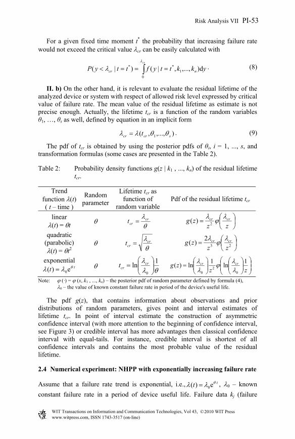
n = 10, ..., 20. The convergence of Bayesian point estimate to the true value is illustrated in Figure 3. Alternative methods for the estimation of the parameter in the model with known trend function are least square method (LSM) and maximum likelihood estimation (MLE). LSM and MLE estimates of the parameters are presented in Figure 3 as well. Note, in this case MLE and BA (with non informative prior) estimates are not equal. The following mean squared errors were calculated: 0.00072 (BA), 0.00159 (MLE), 0.00137 (LSM).

0

0,02

0,04

0,06

0,08

0,1

0,12

9 11 13 15 17 19 21n

BA

MLE

LSM

q* = 0,08

Figure 3: The point estimates of random parameter θ (n = 10, …, 20).

Obviously, if the set of observations is quite big all methods give quite precise estimates of parameters. BA power is the combination of prior (reliable) information and observations (likelihood as well) in the case of few observations (i.e., in the beginning of observation period). The pdf of the failure rate (t) is obtained using the posterior pdf of the parameter and the formula given in Table 1

* = 0.08



n

j

t

jkj

n yytc

kkyf

n

jj

100

1

010

010 exp11

),...,|(

, (11)

n = 10, …, 20, c – normalizing constant, t – time. If the critical value of an increasing failure rate is determined, for instance, cr = 10, the probability that the increasing failure rate will not exceed the critical value cr for a given fixed time moment t* (for instance, t*=24) is 0,935 (obtained using formula (8)). The pdf of the residual lifetime tcr is obtained using the posterior pdf of the parameter and formula given in Table 2

20

cr10 z

1 ln

1),...,|(

ckkzg n

,1

lnexp1

lnexp10 0

cr0

0

cr

10

n

j

n

jj z

jz

kj

(12)

n = 10, …, 20, c – normalizing constant.

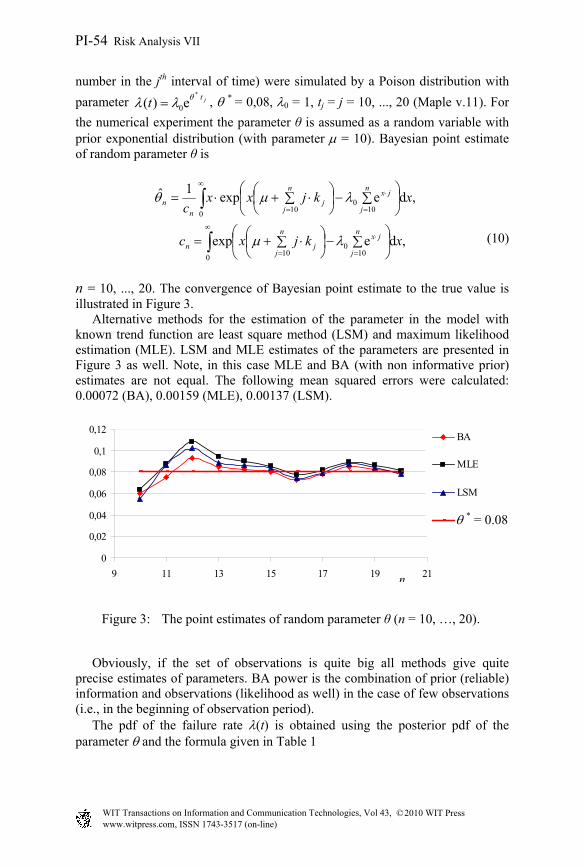
Figure 4: The pdf g(z | k10, ..., k20 ) of the residual lifetime tcr.

The graph of obtained pdf g(z | k10 , ..., k20) is presented in Figure 4. (cr = 10). 95% asymmetric confidence interval of tcr is [22.84; 37.38], i.e., probability P(z < 22.84) = 0.02 and probability P(z > 37.38) = 0.03). The mean value of the residual lifetime 11.29ˆ crt , mode (the most probable value) – 27.32.

A detailed analysis was performed for the evaluation of parameters in a classical nonhomogeneous Poisson process (failure rate depends just on time t) model. The proposed algorithm based on BA modified application is suitable as well in case when failure rate depends on more factors. Performing testing of technical devices (for instance, diesel generators system – part of the emergency power supply system of power reactors [18] or software [1, 19], a Binomial distribution B(N, p) (N – number of trials, p – failure probability) is used as failure distribution. When failures occur more and more frequently a Binomial distribution can be modified: failure probability p is



replaced with an increasing function, for instance, p(t) that depends on time t, or other factors. In this way the Binomial distribution is an appropriate model for the reliability analysis of the testing devices or systems that is in the period of ageing. Estimates of model parameters can be obtained (and updated) by modified application of BA as well.

3 Results and conclusions

This paper presented the developed algorithms (based on Bayesian approach) for the estimation of parameters in mathematical models of non-stationary processes when changes of the process are described by characteristics which means are defined by prior known functional dependencies (for instance, using linear, polynomial, exponential and other trend functions). In case of nonhomogeneous Poisson process, the developed algorithm based on the modification of Bayesian approach application provides obtaining probability distributions of random parameters of system failure rate function. The cases of increasing failure rates with linear, parabolic and exponential

trend functions were analyzed. In the paper illustration of the developed algorithm applicability is presented by numerical experiment: in case when ageing process is characterized by increasing failure rate with prior known trend; it was shown convergence of Bayesian point estimate of parameter of failure rate trend function; obtained results were compared with the ones calculated using least squares method (LSM) – sum of errors squares of LSM is approximately twice bigger than the sum of errors squares of BA.

The algorithm for the assessment of residual lifetime of devices with increasing failure rate (i.e., forecast how long safe operation of device is possible with set dependability level) was developed.

References

[1] Birolini, A. Reliability Engineering. Theory and Practice. 5th.ed.Springer Berlin Heidelberg New York, pp. 323–326, 2007.

[2] Rodionova, A., Atwood, C. L., Kirchsteigera, C., Patrik, M. Demonstration of statistical approaches to identify component’s ageing by operational data analysis—A case study for the ageing PSA network. Reliability Engineering and System Safety, 93, pp. 1534–1542, 2008.

[3] Atwood, C., Cronval, O., Patrik, M., Rodionov, A. Models and data used for assessing the ageing of systems, structures and components (European network on use of probabilistic safety assessment (PSA) for evaluation of ageing effects to the safety of energy facilities). EUR 22483 EN. Petten: EC DG JRC Institute for Energy. 2007

[4] Marshall, A.W., Olkin, I.A. New method for adding a parameter to a family of distributions with application to the exponential and Weibull families. Biometrika 84, pp. 641–52, 1997.

[5] Blischke, W.R., Murthy, D.N.P. Reliability – modeling, prediction and optimization. John Wiley & Sons, Inc, 2002.



[6] Limnios, N., Nikulin, M. Recent Advances in Reliability Theory, Methodology, Practice and Inference. A Birkhauser Boston book. 2000.

[7] Gnedenko, B., Pavlov, I., Ushakov, I. Statistical Reliability Engineering. John Wiley & Sons, Inc., Publications, 1999.

[8] Rausand, M., Høyland, A. System reliability theory – models, statistical methods, and applications. John Wiley & Sons, Inc, 2004.

[9] Murthy, D.N.P., Xie, M., Jiang, R. Weibull Models. John Wiley & Sons, Inc., Publications, 2004.

[10] Crow, D., Feinberg, A. Design for Reliability. CRC Press LLC, 2001. [11] Dodson, B., Nolan, D. Reliability engineering handbook. Marcel Dekker

Inc, 1999. [12] Ireson, W.G., Coombs, C.F., Moss, R.Y. Handbook of reliability

engineering and management. 2nd edition. The McGraw-Hill, Inc, 1996. [13] Yang, B., Xie, M. A study of operational and testing reliability in software

reliability analysis. Reliability Engineering & System Safety. 70(3), pp. 323–329, 2000.

[14] Pham, H. Software reliability. Springer-Verlag Singapure Pte. Ltd, 2000. [15] Huang, C.Y, Lyu, M.R. & Kuo, S.Y. A Unified Scheme of Some

Nonhomogenous Poisson Process Models for Software Reliability Estimation. IEEE Transactions on Software Engineering. 39(3), pp. 261–269, 2003.

[16] Ravishankera, N., Liub, Z. & Rayc, B.K. NHPP models with Markov switching for software reliability. Computational Statistics and Data Analysis. 52, pp. 3988–3999, 2008.

[17] Berthold, M., Hand, D.J. Intelligent Data Analysis. 2nd edition, pp. 138–139, 2003.

[18] Alzbutas, R. Diesel generator system reliability control and testing interval optimization. Energetika, 4, pp. 27–33, 2003.

[19] Peled, D.A. Software reliability methods. Springer-Verlag, 2001. [20] Littlewood, B., Popov, P., Strigini, L. Assessing the reliability of diverse

fault-tolerant software-based systems. Safety Science, Pergamon, 40, pp. 781–796, 2002.



assessment of the system degradation level using the

Documents