assessment of the sales forecast technique double-weighted

http://ijba.sciedupress.com International Journal of Business Administration Vol. 11, No. 2; 2020

Published by Sciedu Press 39 ISSN 1923-4007 E-ISSN 1923-4015

Assessment of the Sales Forecast Technique Double-Weighted Moving

Average vs Other Widely Used Forecasting Techniques

Ma. del Rocío Castillo Estrada1, Marco Edgar Gómez Camarillo1, Fernando Pérez Villaseñor1, Arturo Elías

Domínguez1 & M. Javier Cruz Gómez2

1 Facultad de Ciencias Básicas e Ingeniería y Tecnología, Universidad Autónoma de Tlaxcala, Tlaxcala, Mexico

2 Department of Chemical Engineering, Universidad Nacional Autónoma de México (UNAM), Coyoacán, México

Correspondence: M. Javier Cruz Gómez, Full Professor, Department of Chemical Engineering, Universidad Nacional

Autónoma de México (UNAM), Coyoacán, México.

Received: March 4, 2020 Accepted: March 20, 2020 Online Published: March 30, 2020

doi:10.5430/ijba.v11n2p39 URL: https://doi.org/10.5430/ijba.v11n2p39

Abstract

In order to improve the operations planning of two companies, whose main business is to be chemical products

suppliers in Mexico, it was made the sales forecast of a fourth year of operations, using the monthly sales data

information of the three previous years. The objective of the chemical suppliers forecast was to be in a better position to

satisfy the multiple and varied needs of their clients, which demand different quantities of products and have different

consumption patterns. The sales forecast was made by the next six techniques: Simple Moving Average (SMA),

Weighted Moving Average (WMA), Trend Projection (TP), Exponential Smoothing (ES), Simple Linear Regression

(SLR), and the recently proposed (Castillo, et al. 2016) technique called: Double-Weighted Moving Average

(DWMA). The three years monthly sales data of 61 products, handled by the two companies, were processed in order

to obtain the monthly forecast of the fourth year. After the fourth year, the forecasted data were compared with real

monthly sales data. The analysis was made by the determination of the Symmetric Mean Absolute Percentage Error

(SMAPE), which gave the next results: In the case of company 1, the average errors for the five reference techniques

(SMA, WMA, TP, ES and SLR) was in the range 0.235 – 0.351] vs 0.249 for the DWMA. For company 2, the average

error, of the same five reference techniques was in the range [0.292 – 0.467] vs 0.282 for the DWMA. WMA was the

second technique in giving the least forecasting errors. In both companies, DWMA was the forecasting technique with

one of the lowest average error and the lowest error in most of the products.

Keywords: forecasting techniques, least error, suppliers of chemical products, consumption patterns, operational

planning

1. Introduction

The chemical products supplying companies are characterized by handling high numbers of products, which can vary

between 20 and 500, and a large number of customers, which present different types and forms of business, like:

hardware stores, pharmaceutical enterprises, automotive enterprises, inks and paints producers, and many more. All of

them with different and changing consumption patterns and even with requirements for changes in their last-minute

orders. These circumstances make the chemicals suppliers operations planning to be conducted in a climate of high

uncertainty. So, the development of accurate sales forecasts is an easy and simple way for better operations planning.

Effective planning (Heizer & Render 2009), in the short and long term, depends on the information about the demand

for products that the company has. Good forecasts are crucial for all aspects of the business: the forecast is the only

estimate of demand until real demand is known. Therefore, demand forecasts guide decisions in the areas of human

resources, capacity, inventory control and supply chain management.

It is interesting to realize that, by far, the most successful enterprises use the simplest methodology that also requires

the least amount of data. For Chase and Jacobs (2014), forecasts are vital for any business organization, as well as, for

any important management decision. Forecasts are the basis of long-term corporate planning. In the functional areas of

finance and accounting, forecasts represent the basis for budgeting and controlling costs. With the forecasts, the

marketing staff can make decisions such as, compensation for sales staff, planning of business with new products, etc.

and production/operations staff can make regular decisions about: process selection, production planning, inventory



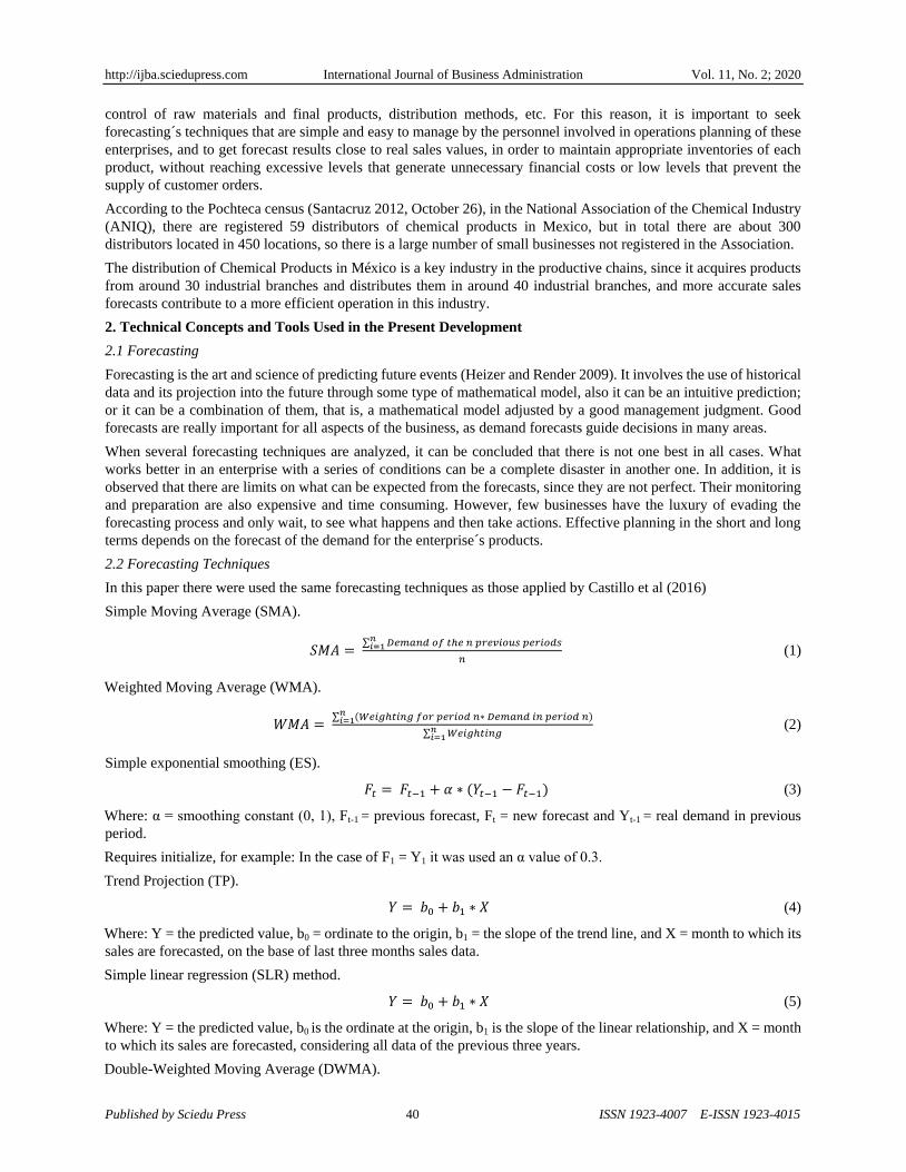
control of raw materials and final products, distribution methods, etc. For this reason, it is important to seek

forecasting s techniques that are simple and easy to manage by the personnel involved in operations planning of these

enterprises, and to get forecast results close to real sales values, in order to maintain appropriate inventories of each

product, without reaching excessive levels that generate unnecessary financial costs or low levels that prevent the

supply of customer orders.

According to the Pochteca census (Santacruz 2012, October 26), in the National Association of the Chemical Industry

(ANIQ), there are registered 59 distributors of chemical products in Mexico, but in total there are about 300

distributors located in 450 locations, so there is a large number of small businesses not registered in the Association.

The distribution of Chemical Products in México is a key industry in the productive chains, since it acquires products

from around 30 industrial branches and distributes them in around 40 industrial branches, and more accurate sales

forecasts contribute to a more efficient operation in this industry.

2. Technical Concepts and Tools Used in the Present Development

2.1 Forecasting

Forecasting is the art and science of predicting future events (Heizer and Render 2009). It involves the use of historical

data and its projection into the future through some type of mathematical model, also it can be an intuitive prediction;

or it can be a combination of them, that is, a mathematical model adjusted by a good management judgment. Good

forecasts are really important for all aspects of the business, as demand forecasts guide decisions in many areas.

When several forecasting techniques are analyzed, it can be concluded that there is not one best in all cases. What

works better in an enterprise with a series of conditions can be a complete disaster in another one. In addition, it is

observed that there are limits on what can be expected from the forecasts, since they are not perfect. Their monitoring

and preparation are also expensive and time consuming. However, few businesses have the luxury of evading the

forecasting process and only wait, to see what happens and then take actions. Effective planning in the short and long

terms depends on the forecast of the demand for the enterprise s products.

2.2 Forecasting Techniques

In this paper there were used the same forecasting techniques as those applied by Castillo et al (2016)

Simple Moving Average (SMA).

∑

(1)

Weighted Moving Average (WMA).

∑ ( )

∑

(2)

Simple exponential smoothing (ES).

( ) (3)

Where: α = smoothing constant (0, 1), Ft-1 = previous forecast, Ft = new forecast and Yt-1 = real demand in previous

period.

Requires initialize, for example: In the case of F1 = Y1 it was used an α value of 0.3.

Trend Projection (TP).

(4)

Where: Y = the predicted value, b0 = ordinate to the origin, b1 = the slope of the trend line, and X = month to which its

sales are forecasted, on the base of last three months sales data.

Simple linear regression (SLR) method.

(5)

Where: Y = the predicted value, b0 is the ordinate at the origin, b1 is the slope of the linear relationship, and X = month

to which its sales are forecasted, considering all data of the previous three years.

Double-Weighted Moving Average (DWMA).



A technique that was proposed by Castillo et al. (2016), based on historical sales data; it considers the variations in

sales values of the last three months and the seasonal behavior of the sales values in last three years, considering

months like the month to be forecasted (for example, for predicting January, there are considered the data of the

previous months of October, November and December and the data of January in the last three years).

DWMA was calculated in following way:

( ( ) ( ) ) (6)

Where: WMA = Weighted moving average.

2.3 Error Calculation

2.3.1 Classification

There are several ways to evaluate forecasting error; these will be described, following the classification stablished by

Hyndman (2016):

There are four types of forecast-error metrics: scale-dependent metrics such as the Mean Absolute Error (MAE), or

Mean Absolute Deviation (MAD); percentage-error metrics such as the Mean Absolute Percent Error (MAPE);

relative-error metrics, which average the ratios of the errors from a designated method to the errors of a naive method;

and scale-free error metrics, which express each error as a ratio to an average error from a baseline method.

For assessing accuracy on a single series, the MAE metric is preferred because it is easiest to understand and compute.

However, it cannot be compared across series because it is scale dependent.

Percentage errors have the advantage of being scale independent, so they are frequently used to compare forecast

performance between different data series. But measurements based on percentage errors have the disadvantage of

being infinite or undefined if there are zero values in a series, as is frequent for intermittent data.

Relative-error metrics are also scale independent. However, when the errors are small, as they can be with intermittent

series, use of the naïve method as a benchmark is no longer possible because it would involve division by zero.

The scale-free error metric called Mean Absolute Scaled Error (MASE) can be used to compare forecast methods on a

single series and also to compare forecast accuracy between series. This metric is well suited to intermittent-demand

series because it never gives infinite or undefined values.

The SMAPE, proposed by Makridakis in 1993, is a modified Mean Absolute Percentage error (MAPE), in which the

divisor is half of the sum of the real and forecasted values. SMAPE can be applied when the demand is intermittent,

since the error technique can handle the zero demand without approaching infinity.

2.3.2 Tried out Methods for Error Calculation

Due to the importance of error calculation for this work, different alternative methods were tried to measure the error of

the predictions, starting by testing the MAPE which is defined as:

∑ | |

(7)

Where At and Ft denote the current and predicted values at data point t, respectively, and n is the number of data points.

We found calculation problems where the monthly sales values equal to zero or very close to zero, that s why

calculated errors would be infinite or extremely high numbers, this situation coincides with what was expressed by S.

Kim and H. Kim (2016), and it is transcribed below:

The MAPE is one of the most popular measures of forecast accuracy. It is recommended in most textbooks for example,

Bowerman, O'Connell and Koehler (2004), Hanke and Reitsch (1995), and was used as the main measure in the M

competence (M is the name given to a competition of different forecasting techniques, because the organizer was

Makridakis) (Makridakis et al., 1982). MAPE is the mean of Absolute Percentage Errors (APE).

It was tried to solve the problem of sales values equal to zero or very close to zero, by excluding outliers that have real

values less than one, or APE values greater than the MAPE plus three standard deviations (Makridakis, 1993).

However, this approach is only an arbitrary adjustment, and leads to another question, namely, how outliers can be

eliminated. In addition, the exclusion of outliers can distort the information provided, particularly when the data

involves numerous small real values. Several alternative measures have been proposed to address this problem. For

example, the SMAPE, proposed by Makridakis (1993). It is a modified MAPE in which the divisor is half the sum of

the actual and predicted values.



While S. Kim and H. Kim (2016), commented on other alternative methods, they proposed a new way to measure the

errors in the prognoses called mean arc tangent absolute percentage error (MAAPE).

In the present research, for error calculation, it was used the SMAPE, defined in the next equation 8:

∑ | |

∑ ( )

(8)

Where: At is the real value, Ft is the predicted value.

2.4 Selecting Forecasting Methods

Armstrong (2001) examined six parameters to select forecasting methods: convenience, market popularity, structured

judgment, statistical criteria, relative track records, and guidelines from prior research.

Convenience

In many situations, it is not worth spending a lot of time to select a forecasting method. Sometimes little change is

expected, so different methods will yield similar forecasts. Or perhaps the economics of the situation indicate that

forecast errors are of little consequence. These situations are common.

Convenience may lead to methods that are hard to understand. Statisticians, for example, sometimes use Box-Jenkins

(2015) procedures to forecast because they have been trained in their use, although decision makers may be mystified.

This methodology is applied in the analysis of time series, it uses the Auto Regressive Mobile Average (ARMA),

models, or the Auto Regressive Integrated Mobile Average (ARIMA), models to find the best fit for a time series of

values, so that the forecasts are more accurate.

Also, a method selected by convenience may lead to large errors in situations that involve large changes.

Market popularity

Market popularity involves determining what methods are used by other people or organizations. The assumptions are

that (1) over time, people figure out what methods work best, and (2) what is best for others will be best for you.

Surveys of usage, offer only indirect evidence of success.

Structured judgment

When a number of criteria are relevant and a number of methods are possible, structured judgment can help the

forecaster to select the best methods. In structured judgment, the forecaster first develops explicit criteria and then rates

the methods.

Statistical criteria

Statisticians rely heavily upon whether a method meets statistical criteria, such as the distribution of errors, statistical

significance of relationships, or an autocorrelation test in the residuals of a statistical regression analysis, like the

Durbin-Watson (DW), (1971) statistic.

Statistical criteria are not appropriate for making comparisons among substantially different methods. They would be

of little use to someone trying to choose between judgmental and quantitative methods, or among role playing and

expert forecasts. Statistical criteria are useful for selection only after the decision has been made about the general type

of forecasting method, and even then, their use has been confined primarily to quantitative methods.

Relative track records

The relative track record is the comparative performance of various methods as assessed by procedures that are

systematic, unbiased, and reliable. It does not have to do with forecasting methods being used for a long time or

people’s satisfaction with them.

Principles from published research

Assume that you need to forecast personal computer sales in China over the next ten years. To determine which

forecasting methods to use, you might use methods that have worked well in similar situations in the past. Having

decided on this approach, you must consider: (1) How similar were the previous situations to the current one? (You

would be unlikely to find comparative studies of forecasts of computer sales, much less computer sales in China), (2)

Were the leading methods compared in earlier studies? (3) Were the evaluations unbiased? (4) Were the findings

reliable? (5) Did these researchers examine the types of situations that might be encountered in the future? and (6) Did

they compare enough forecasts?



An extensive body of research is available for developing principles for selecting forecasting methods. The principles

are relevant to the extent that the current situation is similar to those examined in the published research. Use of this

approach is fairly simple and inexpensive.

General Principles

Use structured rather than unstructured forecasting methods

Use quantitative methods rather than judgmental methods if enough data exist.

Use causal rather than naive methods, especially if changes are expected to be large.

Use simple methods unless substantial evidence exists that complexity helps.

Match the forecasting methods to the situation.

In this work, we focused in accuracy for selecting more suitable forecasting method.

3. Methodology

In this work, we look for demand patterns and try to find different demand components that could help us to establish a

correlation between demand patterns and the lower error forecasting technique. Chase and Jacobs (2014), in relation to

the components of the demand, state following. In most cases, the demand for products or services is divided into six

components: average demand for the period, a trend, seasonal elements, cyclical elements, random variation and

autocorrelation.

It is more difficult to determine the factors because perhaps the time is unknown or the cause of the cycle is not

considered. The cyclical influence on demand can come from events such as political elections, wars, economic

conditions or sociological pressures.

Random variations are caused by fortuitous events. Statistically by subtracting all known causes of demand (average,

trends, seasonal, cyclical and autocorrelation) from total demand, what remains is the inexplicable part of demand. If

the cause of the remainder cannot be identified, it is assumed to be random.

The autocorrelation indicates the persistence of the fact. More specifically, the expected value at one time has a very

high correlation with its own previous values. In the theory of the waiting line, the length of a waiting line has a very

high autocorrelation. That is, if a line is too long at a certain time, shortly after that time it would be expected that the

line would remain long.

The software "System for predicting sales for suppliers of chemicals”, developed by Abascal, et al. (2016), was used

for evaluating different forecasting techniques on the basis of historical sales of Chemical Products Supplying

Enterprises, comparing forecasting results with actual sales. The software only requires historical sales information of

three years to make the forecast and sales information of a fourth year. To assess the accuracy of the forecast, both the

most popular method for calculating errors, the mean absolute percentage error (MAPE), as well as the symmetric

mean absolute percentage error (SMAPE), were used. The first one was discarded because it gave error values to high

when real sales were close to zero, and infinite error values when real sales were zero. On the contrary the second

method results indicated that it is more appropriate to assess the characteristics of historical sales data.

The program was used with the sales data (fifty products of the company 1 and eleven products of the company 2,

which represented about 80% of total sales volume in both cases) of the first three years, the graphs of monthly sales vs

months were generated, in order to be able to analyze the type of pattern presented by the sales in each case. Then, sales

forecast calculations were performed using the techniques SMA, WMA, TP, ES, SLR and DWMA. Subsequently,

errors were calculated for each technique, each product and each company, comparing forecasted values vs real sales

data. Error results were analyzed to establish which techniques presented the least error in most of the products. The

sales graphs of each product were analyzed in order to find the relationship between the sales patterns and the forecasts

calculated with the lower error technique.

4. Research Results

The errors for each product, each forecasting technique and each of the two companies are shown in Tables 1 and 2.



Table 1. Forecasting error for Company 1 products

Product DWMA SMA WMA TP ES SRL

1 0.0575 0.0776 0.0709 0.0910 0.0816 0.0659

2 0.2303 0.2322 0.2184 0.3024 0.2451 0.3963

3 0.3374 0.3550 0.3600 0.6115 0.3249 0.3684

4 0.2748 0.2990 0.2927 0.4831 0.3002 0.4904

5 0.3662 0.3439 0.3273 0.3545 0.3378 0.5106

6 0.2542 0.3159 0.2945 0.3594 0.3098 0.2668

7 0.7074 0.6796 0.6075 1.4414 0.7366 0.8046

8 0.0957 0.0842 0.0850 0.1301 0.0921 0.1291

9 0.2596 0.1715 0.1649 0.2339 0.1759 0.6107

10 0.1286 0.1323 0.1350 0.1669 0.1212 0.1146

11 0.2513 0.2858 0.2722 0.3755 0.2443 0.2409

12 0.2140 0.2444 0.2570 0.5434 0.2539 0.2986

13 0.1406 0.0986 0.0975 0.1409 0.1005 0.1784

14 0.2350 0.1987 0.1906 0.2656 0.1886 0.1597

15 0.1523 0.1537 0.1531 0.2250 0.1369 0.8043

16 0.2840 0.2002 0.1885 0.2034 0.1970 0.7559

17 0.2036 0.1620 0.1560 0.2089 0.1743 0.1159

18 0.4083 0.3425 0.3165 0.3849 0.3704 0.8292

19 0.2204 0.0756 0.0855 0.2043 0.0836 0.2682

20 0.3135 0.1983 0.1827 0.2118 0.2166 0.6214

21 0.2794 0.3122 0.2960 0.3226 0.3352 0.3073

22 0.1688 0.1062 0.1028 0.1373 0.1077 1.0703

23 0.4555 0.5857 0.5061 0.7089 0.6016 1.0116

24 0.1322 0.0978 0.0982 0.1846 0.1031 0.1319

25 0.1347 0.1709 0.1530 0.1463 0.1782 0.1857

26 0.2279 0.1697 0.1904 0.3746 0.1797 0.4038

27 0.3538 0.3864 0.3484 0.5349 0.3515 0.3334

28 0.0943 0.1298 0.1279 0.1662 0.1339 0.1242

29 0.3813 0.4062 0.4480 0.8884 0.4015 0.5275

30 0.1743 0.1516 0.1395 0.1859 0.1614 -8.1482

31 0.1293 0.1365 0.1348 0.1823 0.1287 0.2035

32 0.2145 0.1657 0.1612 0.3091 0.1688 0.2723

33 0.2761 0.2846 0.2858 0.4969 0.2778 0.2379

34 0.2110 0.1526 0.1476 0.1696 0.1422 0.2578

35 0.1719 0.1979 0.1965 0.2468 0.1954 0.1540

36 0.3237 0.3528 0.3316 0.4593 0.3666 0.2940

37 0.2165 0.2188 0.2293 0.3600 0.1844 0.1291

38 0.3811 0.2828 0.2783 0.3815 0.2757 0.3849



39 0.2969 0.2345 0.2167 0.4605 0.2522 0.5730

40 0.3291 0.1923 0.1753 0.2195 0.2090 0.5138

41 0.2444 0.2816 0.2813 0.3626 0.2985 3.1235

42 0.1790 0.1784 0.1746 0.2425 0.1723 0.5371

43 0.3087 0.3992 0.3935 0.5486 0.3905 0.2943

44 0.3540 0.5387 0.5148 0.6661 0.5288 0.4775

45 0.0869 0.1146 0.1245 0.2173 0.1174 0.1135

46 0.2075 0.2672 0.2790 0.3645 0.2848 0.2983

47 0.2376 0.1460 0.1473 0.2017 0.1651 0.4829

48 0.2888 0.3631 0.3604 0.4767 0.3553 0.3419

49 0.1499 0.2050 0.1923 0.2389 0.2024 0.2905

50 0.3330 0.3125 0.2975 0.3701 0.3350 0.6903

Average 0.2495 0.2438 0.2358 0.3512 0.2459 0.2729

Table 2. Forecasting error for Company 1 products

Product DWMA SMA WMA TP ES SLR

1 0.0665 0.0696 0.0704 0.1033 0.0659 0.0705

2 0.1870 0.2719 0.2649 0.3751 0.2528 0.3756

3 0.0803 0.0914 0.0948 0.1803 0.1029 0.0843

4 0.0941 0.1121 0.1044 0.1105 0.1162 0.1187

5 0.1112 0.0761 0.0746 0.0978 0.0721 0.1591

6 0.1493 0.1561 0.1617 0.3453 0.1575 0.1657

7 0.7262 0.7646 0.7629 1.0745 0.7462 0.6240

8 0.5903 0.5709 0.5608 0.8574 0.5904 0.5450

9 0.5227 0.6158 0.6615 1.0760 0.6342 0.5647

10 0.3201 0.2478 0.2629 0.4383 0.2558 0.4586

Average 0.2825 0.2925 0.2997 0.4673 0.2979 0.3143

The analysis of the SMAPE average errors for the different forecasting techniques, for all the products of each

company, allowed locating the DWMA as the technique in which, for the greatest number of products, it was obtained

the smallest prediction error: Fifteen of fifty products for company 1 and five of eleven products for company 2. The

DWMA technique presents not only the lower error levels, but also the lower dispersion of the error values, as it is

shown in Figures 1 and 2.



Figure 1. Chart for company 1 showing SMAPE error levels and dispersion for each forecasting technique, considering

fifty products

Figure 2. Chart for company 2 showing SMAPE error levels and dispersion for each forecasting technique, considering

eleven products

For products in which the DWMA technique was obtained as a minor error technique, demand patterns exhibited

during the previous three years were analyzed, and it was found that sales show a combined pattern of trend and

cyclicity. Figure 3 with sales values of product 1, company 1 is an example of a combined pattern of trend and cyclicity,

it has a series of maximum sales peaks uniformly distributed during each year, combined with a tendency to reduce the

volume of sales i.e. in the last two years a slightly decreasing trend has been presented, with peaks of higher sales in the

first and third quarters of each year. Figure 5, shows the demand of product 28, company 1. In here the seasonal peaks

are not so clear but it can be observed a tendency for reducing sales level and again some peaks of higher sales. In this

second case, the lower error forecasting technique, was also DWMA. Figures 4 and 6 show a comparison between

actual sales and forecasted sales for the fourth year, based on the data shown in Figures 3 and 5 respectively.

1

0

0.2

0.4

0.6

0.8

1

1.2

DWMA. SMA. WMA. TP. ES. SLR

1

0

0.2

0.4

0.6

0.8

1

1.2

DWWMA SMA. WMA. TP.



Figure 3. Monthly sales data of three years for company 1 and product 1

Figure 4. Comparison between actual sales and forecasted sales in fourth year; company 1, product 1

0

100000

200000

300000

400000

500000

600000

0 1 2 3 4 5 6 7 8 9 10 11 12 13 14 15 16 17 18 19 20 21 22 23 24 25 26 27 28 29 30 31 32 33 34 35 36

Company 1, Product 1

Months

Kg/

mo

nth

150000

200000

250000

300000

350000

400000

450000

0 2 4 6 8 10 12 14


Sales data DWMA

Kg/

mo

nth

Months





For the analysis of the second enterprise in 5 of 11 products, in which a combined trend pattern and uniformly

distributed sales peaks are also evident during the year, the lowest error technique was also DWMA. Two typical cases

are presented in what follows. For company 2, product 1, the tendency was to increase sales in about a hundred

thousand kg/year, combined with sales peaks evenly distributed through the year, see Figure 7 for monthly sales data of

three years, and Figure 8 for the forecasted and real sales of the fourth year. This forecast did not give a further increase

0

10000

20000

30000

40000

50000

60000

0 1 2 3 4 5 6 7 8 9 10 11 12 13 14 15 16 17 18 19 20 21 22 23 24 25 26 27 28 29 30 31 32 33 34 35 36


Months

Kg/

mo

nth

0

5000

10000

15000

20000

25000

30000

35000

40000

45000

50000

0 2 4 6 8 10 12 14


Sales data 28 DWMA

Kg/

mo

nth

Months



of an extra hundred thousand kg/year for the fourth year, that a SLR technique will predict. The DWMA prediction was

closer to the real sales. In the case of company 2, product 3, the tendency was to maintain a constant sales level,

combined with peak sales at the beginning and end of the year, see Figure 9 for monthly sales data of three years and

Figure 10 for the forecasted and real sales of the fourth year.



0

100000

200000

300000

400000

500000

600000

700000

800000

900000

0 1 2 3 4 5 6 7 8 9 10 11 12 13 14 15 16 17 18 19 20 21 22 23 24 25 26 27 28 29 30 31 32 33 34 35 36


Months

Kg

/mo

nth

400000

500000

600000

700000

800000

900000

1000000

0 1 2 3 4 5 6 7 8 9 10 11 12


Real sale DWMA

Kg/

mo

nth

Months




Figure 10. Comparison between actual sales and forecasted sales for the fourth year of company 2, product 3

The monthly sales data for three years, showed in Figures 11 and 13, are examples of a decreasing or increasing

tendency, but higher sales peaks cannot be clearly identified. In this case was the WMA technique that gave the

forecasts with closer to real sales values. Figures 12 and 14 show the comparisons between actual sales, and expected

sales based on data from the previous two figures. In the same company 1 other products presented trend, but no sales

peaks with some frequency, in all these cases the WMA technique gave the forecasts with closer to real sales values.

0

50000

100000

150000

200000

250000

300000

350000

400000

450000

500000

0 1 2 3 4 5 6 7 8 9 10 11 12 13 14 15 16 17 18 19 20 21 22 23 24 25 26 27 28 29 30 31 32 33 34 35 36


Months

Kg/

mo

nt

100000

150000

200000

250000

300000

350000

0 1 2 3 4 5 6 7 8 9 10 11 12

Company 2, product 3

Real sale DWMA

Kg/

mo

nth

Kg/month





0

50000

100000

150000

200000

250000

300000

0 1 2 3 4 5 6 7 8 9 10 11 12 13 14 15 16 17 18 19 20 21 22 23 24 25 26 27 28 29 30 31 32 33 34 35 36


Months

Kg/

mo

nth

100000

120000

140000

160000

180000

200000

220000

240000

0 1 2 3 4 5 6 7 8 9 10 11 12

Company1, Product 8

Sales data 8 DWMA

Kg/

mo

nth

Months





By doing the sales forecast with the six techniques described in this paper and calculating the average error for each

forecast of all the 50 chemical products, of company 1, it was made an assessment of the relative usefulness of each

technique. DWMA was the first and WMA was the second technique in giving the least forecasting errors. In figure 15,

it is shown how with DWMA and WMA in 29 of 50 company 1 products, it is obtained the least farecasting error. With

respect to the products (14 of 50 in company 1) in which the WMA technique was obtained as the least error technique,

0

50000

100000

150000

200000

250000

300000

0 1 2 3 4 5 6 7 8 9 10 11 12 13 14 15 16 17 18 19 20 21 22 23 24 25 26 27 28 29 30 31 32 33 34 35 36


Months

Kg/

mo

nth

100000

120000

140000

160000

180000

200000

220000

240000

0 1 2 3 4 5 6 7 8 9 10 11 12

Company1, Product 8

Sales data 8 DWMA

Kg/

mo

nth

Months



the analysis of the demand, exhibited by the three-year monthly sales data, shows only a trend pattern. In Figure 16 are

shown, for company 2 products, the number of products that gave for each forecasting technique the least errors. With

the DWMA technique it was obtained in 5 of the 11 products the least farecasting error.

Figure 15. Chart for Company 1 showing forecasting techniques with lowest error in fifty products

Figure 16. Chart for Company 2 showing forecasting techniques with lowest error in eleven products

In summary, with the two forecasting methods: The DWMA and the WMA, in 56% of the products, distributed in the

two companies, the smallest forecast errors are obtained. In addition, by using the already mentioned software, it is

possible to select the forecasting technique with less error, for all products in a simple and fast way, and establish a

relationship between the demand pattern and the most appropriate forecasting technique.

5. Discussion

For selecting a suitable forecasting method, Chase and Jacobs, (2014) proposed the guide summarized on Table 3.



Table 3. Guide for selecting a suitable forecasting method

Forecasting method Quantity of historical data Data pattern Forecast horizon

Linear regression From ten to twenty

observations for

temporality, at least five

observations per season

Stationary, trend and

temporality

Short to medium

Simple moving average Six to twelve months,

weekly data is often used

The data must be

stationary (i.e. without

trend or temporality)

Short

Weighted moving

average and Simple

exponential smoothing

To begin with, five to ten

observations are needed

The data must be

stationary

Short

Exponential smoothing

with trend

To begin with, five to ten

observations are needed

Stationery and trends Short

Although the guide mentions that in order to select the WMA method the data pattern should be seasonal, in our case

this technique was adequate in trend patterns.

The guide does not mention the DWMA because this technique was proposed in 2016, two years after the Chase and

Jacobs paper, however, it mentions linear regression as adequate for stationary, trends and temporality data patterns, in

this work the DWMA was found to be more adequate than linear regression, for seasonal and trend type data patterns.

Establishing the best forecasting method for the sales, of a sector of the Economy as broad and changing as that of the

distribution of chemical products, is not an easy job, and in addition, a method selected as the least error in a specific

year, it may not be the most appropriate in another period of time. That is why, it is important to repeat the data analysis

at least annually to verify if sales patterns are maintained, and if there are variations, to determine again which is the

best forecasting method to be used for each product in the new scenario.

For selecting forecasting methods, regarding six ways analyzed by Amstrong (2001), in this work we made the

following considerations:

Convenience

When examining the forecasts that companies have already made, it was found that company 1 uses the SMA

technique, and company 2 uses the TP technique, for all their respective products. Although, it could be convenient to

use the forecasting methods selected by each company to take advantage of personnel experience, for this research, it

was decided to compare the two mentioned methods with the other four, looking for the more suitable one in each

company. By using the appropriate software and making the graphic evaluation of the forecasted values it is easy to

define the best method to use. This exercise also helps the decision makers in the development of their work.

Market popularity

In this work there were used 5 popular methods, that many companies use because they are easy to understand and to

handle, and the DWMA method.

Structured judgment

With respect to the criteria used for selecting the more suitable forecasting methods, it was chosen the forecasting with

least error for one-year period, and then it was compared in a graphic way the real sales data vs forecasted data by the

selected method.

Statistical criteria

The forecasting techniques that have the least error in the largest number of products were selected, and the results

reflected in a Pareto Chart as in Figures 1 and 2. By considering all products in both companies and using Boxplot

Charts, as in Figures 15 and 16, it was found that DWMA technique presented the lowest error level.

Relative track records

The comparative performance of the six methods was evaluated by analyzing, the demand patterns of each product

over a period of three years; with the data it was made the sales forecast for a fourth year, using six methods. These



forecasts were compared with the actual sales data for the fourth year, and the SMAPE error was calculated in each

case.

Principles from published research

We did not find a published research for selecting forecasting methods specifically applied to Chemicals suppliers, but

we found different papers talking about selecting or evaluating forecasting methods in other economic activities.

According to Chase and Jacobs (2014) the forecast model that an enterprise must choose depends on:

1. The time horizon that is going to be forecasted.

In the present research there were made monthly forecasts for an annual sales period, for each product, and each

enterprise.

2. The availability of data.

It was available the monthly sales data of products sold by two companies that supply chemical products,

corresponding to four annual periods.

3. The required precision.

It was established the objective of identifying the most accurate forecasting method (s) in each case, through the use of

the software already mention in this paper.

4. As for the budget for forecasts.

Only a relatively small budget is required to make the forecasts, by the use of the above-mentioned software that can be

run in any operating system (Windows, Mac or Unix).

5. The availability of qualified personnel

With respect to the availability of qualified personnel, the use of the aforementioned software is simple and fast, and

specialized personnel in statistics, models or computing are not required. It carries out both the analysis of sales

patterns of chemical suppliers based on historical data from three years prior to the desired one, as well as the selection

of the predictive method that may have the least error in each product; and after the fourth year it is possible to make

the comparison of the forecasted values against the actual sales data, and the calculation of the monthly errors. By

annually doing this exercise, it is possible to notice any change in the demand patterns of the products, and make a new

selection of the best forecasting technique.

6. Conclusions

The obtained results allow us to conclude that; although each product has a forecasting method with the lowest error

compared to real sales, this method of forecasting least error can change with time. Also, it was observed that two of

the six compared methods, DWMA and WMA gave the results of the lowest error in 57% of the products. In other

words, the sales of most products in this sector of the economy, present patterns with increasing or decreasing trends

and at the same time seasonal peaks (each year in the same quarter) of higher or lower sales. For this type of patterns,

the two methods mentioned above offer the closest forecast to real sales values.

We also must say that we found that the DWMA forecast technique, gave good results in about 34.5% of all

analyzed products and that the demand patterns of these products tended to increase or decrease the level of sales or

even to remain at a constant level, but presenting peaks of repetitive sales in any particular month or quarter of each

year.

Taking into consideration that most of the companies supplying chemical products in Mexico, are small companies

that need to make forecasts of their sales as accurate as possible for planning their operations, but usually these

companies do not have specialized personnel, the evaluation of simple forecasting methods, looking for the least

error depending on the type of demand patterns of each product, represents a viable option.

Finally, it is clear that the more products a company manages, the more calculations will be necessary, so the use of

software such as the one used in this work will be useful for the calculation and analysis process to be carried out in a

relatively short time.



References

Abascal, L. O., Castillo, M. del R., & Cruz, M. J. (2016). Sistema para la predicción de ventas de empresas

proveedoras de productos químicos. Instituto Nacional del Derecho de Autor. México.

Armstrong, J. S. (1985). Long-range forecasting: from crystal ball to computer (2nd ed.). New York, Wiley.

Armstrong, J. S. (2001). Selecting Forecasting Methods. Retrieved from

http://repository.upenn.edu/marketing_papers/147

Box, G. E. P., & Jenkins, G. M. (2015). Time series analysis: forecasting and control (5th ed.). Published by John

Wiley and Sons Inc.

Byrne, R. F. (2012). Beyond traditional time-series: Using demand sensing to improve forecasts in volatile times.

The Journal of Business Forecasting, 31, 13

Castillo, M., del Rocío, C. M., Del Rio, R., & Cruz, G. M. J. (2016). Double weighted moving average: alternative

technique for chemicals supplier s sales forecast. International Journal of Business Administration, 7(4), 58-69.

https://doi.org/10.5430/ijba.v7n4p58

Chase, R. B., & Jacobs, F. R. (2014). Administración de operaciones producción y cadena de suministros. México

D.F.: Mc Graw Hill / Interamericana Editores SA de CV

Durbin, J., & Watson, G. S. (1971). Testing for Serial Correlation in Least Squares Regression. III. Biometrika, 58(1),

1-19. Retrieved February 21, 2020, from www.jstor.org/stable/2334313

Hanke, J. E., & Reitsch, A. G. (1995). Business forecasting (5th ed.). Englewood Cliffs, NJ: Prentice-Hall.

Heizer, J., & Render, B. (2009). Principios de Administración de Operaciones. México, D.F.: Pearson Educación.

Hyndman, R. J. (2006, June). Another look at forecast-accuracy metrics for intermittent demand. Retrieved from

https://robjhyndman.com/papers/foresight.pdf

Kim, S., & Kim, H. (2016). A new metric of absolute percentage error for intermittent demand forecasts.

International Journal of Forecasting, 32(2016), 669-679, https://doi.org/10.1016/j.ijforecast.2015.12.003

Makridakis, S. (1993). Accuracy measures: theoretical and practical concerns. International Journal of Forecasting,

9, 527-529

Makridakis, S., Anderson, T. O., Carbone, R., Fildes, R., Hibon, M., & Lewandowski, R. (1982). The accuracy of

extrapolation (time series) methods: Results of a forecasting competition. Journal of Forecasting, 1, 111-153

Makridakis, S., Wheelwright, S., & Hyndman, R. J. (1998). Forecasting: Methods and applications (3rd ed.). New

York, John Wiley and Sons.

Santacruz, A. (2012, Octubre 26). Situación actual y perspectivas de la distribución de productos químicos en

México [PowerPoint slides]. Retreived from

http://www.aniq.org.mx/foro/2012/pdf/7%20QUINTA%20SESION%20PLENARIA/4.-Armando%20Santacruz

Presentacion%20%20distribucion%20Mexico%20final%20(5%200).pdf

assessment of the sales forecast technique double-weighted

Documents