assessment of gas-surface interaction models for computation...
TRANSCRIPT

ASSESSMENT OF GAS-SURFACE INTERACTION MODELS FOR COMPUTATION OF RAREFIED
HYPERSONIC FLOWS
by
Jose Fernando Padilla
A dissertation submitted in partial fulfillment of the requirements for the degree of
Doctor of Philosophy (Aerospace Engineering)
in The University of Michigan 2008
Doctoral Committee: Professor Iain D. Boyd, Chair Professor Philip L. Roe Professor Kenneth G. Powell Associate Professor Hong G. Im

© Jose Fernando Padilla All rights reserved
2008
ii
ACKNOWLEDGEMENTS
First, I acknowledge and thank God. Second, I thank my advisor and chair of my
thesis committee, Iain Boyd. He helped me to enter the program, stay with the program
and finish within an adequate time period; he was instrumental in acquiring funding for
the program; he introduced me to professional society conferences and journal paper
submission; he connected me with external scholars and professionals; and he helped me
find employment. Third, I acknowledge the sponsorship by the Space Vehicle
Technology Institute, under the National Aeronautics and Space Administration (NASA)
grant NCC-3989 with joint sponsorship from NASA and the Department of Defense.
Fourth, I thank the rest of my dissertation committee: Philip Roe for his suggestions on
technical writing, and Kenneth Powell and Hong Im, also for their cooperation, allowing
me to finish the doctoral program. Fifth, I thank the following scholars and professionals
for contributing data to the analysis in this thesis: from the University of Virginia, Eric
Cecil and his mentor James McDaniel for their laser induced fluorescence measurements,
and from NASA, James Moss for his computational simulation data and David Hash for
his suggestions on an Earth atmosphere model. Sixth, I acknowledge the professors who
taught my core courses or administered my preliminary exams: Bernal, Boyd, Dahm,
Driscoll, Faeth, Gallimore, Powell, Roe and van Leer. Seventh, I acknowledge the

iii
following colleagues for their help or otherwise “moral” support: John, Jon, Jeremy,
Tom, Andrew, Leo, Chunpei, Anton, Alexandre, Andy, Dave, Quanhua, Wen-Lan, Matt
and Justin. For other colleagues of Boyd’s research group, I encourage them in their
endeavors. Finally, I acknowledge and thank my parents, siblings and friends for their
support.

iv
TABLE OF CONTENTS
ACKNOWLEDGEMENTS ...................................................................................... ii
LIST OF FIGURES .................................................................................................. vii
LIST OF TABLES .................................................................................................... xi
CHAPTER
I. INTRODUCTION ...................................................................................... 1
1.1 Motivation .................................................................................... 1
1.2 A History of Hypersonics Research .............................................. 4
1.3 Computational Methods for Hypersonic Flow ............................... 8
1.3.1 Pre electronic digital computer methods ....................... 8
1.3.2 Continuum computational methods............................... 10
1.3.3 Kinetic computational methods .................................... 13
1.4 Objective and Overview ............................................................... 16
II. GENERAL SIMULATION PROCEDURES ............................................ 18
2.1 Overview of the DSMC Method ................................................... 18
2.2 Description of the MONACO DSMC Code .................................. 22
2.3 General DSMC Grid Generation Procedure .................................. 24
2.4 Overview on Post Processing ........................................................ 28
III. ASSESSMENT OF AERODYNAMICS MODELING AND
WINDTUNNEL DATA .............................................................................. 31
3.1 Background and Relevance ........................................................... 31
3.2 Analytical Flow Approximations .................................................. 32
3.2.1 Flow regime and relevance ........................................... 32
3.2.2 Modified Newtonian flow ............................................. 33
3.2.3 Free molecular flow ...................................................... 35
3.3 Aerodynamic Force Integration .................................................... 38
3.4 Blunted Cone Simulations ............................................................ 43

v
3.4.1 Flow conditions and geometry ...................................... 43
3.4.2 Results and discussion .................................................. 45
3.5 Apollo Command Module Simulations ......................................... 51
3.5.1 Flow conditions and geometry ...................................... 51
3.5.2 Results and discussion .................................................. 53
3.6 Axisymmetric Simulations ............................................................ 57
3.6.1 Flow conditions and geometry ...................................... 57
3.6.2 Results and discussion .................................................. 59
3.7 Chapter Summary and Conclusions .............................................. 63
IV. SENSITIVITY OF AEROTHERMODYNAMICS PREDICTIONS
FOR APOLLO 6 RETURN AT 110 km ALTITUDE ............................... 66
4.1 Background .................................................................................. 66
4.2 General Description of the Simulations ......................................... 68
4.3 Sensitivity to Surface Conditions .................................................. 70
4.3.1 Effects on maximum field and wall temperatures .......... 72
4.3.2 Effects on ACM aerodynamics and surface heating ...... 80
4.4 Sensitivity to Chemically Reacting Flow ...................................... 83
4.5 Chapter Summary and Conclusions .............................................. 87
V. ASSESSMENT OF GAS-SURFACE INTERACTION MODELS .......... 90
5.1 Introduction .................................................................................. 90
5.2 A Chronicle of Models since Maxwell .......................................... 92
5.3 Mathematical Description of Two Modeling Concepts ................. 99
5.3.1 Interaction parameters .................................................. 99
5.3.2 Scattering kernel ........................................................... 100
5.4 Mathematical Description of Two Common Models in Use with
DSMC .......................................................................................... 101
5.4.1 Maxwell model............................................................. 101
5.4.2 Cercignani, Lampis and Lord model ............................. 102
5.5 Flat Plate Windtunnel Test Simulations Using the Two Models .... 103
5.5.1 General description....................................................... 103
5.5.2 Comparisons with compressible boundary layer
theory ........................................................................... 106
5.5.3 Contour plots ................................................................ 112
5.5.4 Effects of gas-surface accommodation on molecular
probability distributions ................................................ 113
5.5.5 Effects of gas-surface accommodation on boundary
layer velocity profiles ................................................... 116
5.5.6 Seeded iodine simulations ............................................ 121
5.5.7 Analysis of thermal nonequilibrium in the boundary
layer ............................................................................. 129

vi
5.6 Apollo 6 Flight Simulations Using the Two Models ...................... 141
5.7 Chapter Summary and Conclusions .............................................. 145
VI. GENERAL SUMMARY AND FUTURE WORK .................................... 149
Overview ...................................................................................... 149
Summary of Results and Conclusions ........................................... 150
Suggestions for Future Work ........................................................ 153
6.3.1 Program processing ...................................................... 153
6.3.2 Gas-surface interaction modeling.................................. 156
6.3.3 Simulation studies involving comparisons with real
physical data ................................................................. 157
BIBLIOGRAPHY ..................................................................................................... 159
vii
LIST OF FIGURES
Figure
1.1 History of documents containing “hypersonic” in the title, abstract or
subject [Engineering Village (2007)] ........................................................... 5
1.2 Percentage of documents of Fig. 1.1 containing “computation”,
“numerical” or “simulation” in the title, abstract or subject [Engineering
Village (2007)] ............................................................................................ 6
2.1 Computational grid generation for seeded iodine simulation ........................ 27
3.1 Surface element of Newtonian flow ............................................................. 34
3.2 Surface element of free molecular flow ........................................................ 36
3.3 Blunted-cone integration regions ................................................................. 40
3.4 Validation of element summation integration procedure against integral
equations using free molecular flow analysis for the blunted-cone at
Ma = 9.56 .................................................................................................. 42
3.5 Blunted-cone geometry ................................................................................ 44
3.6 Domain boundary for simulation of blunted-cone at a 20 angle-of-attack ... 45
3.7 Contour plot of translational temperature at symmetry boundary of three-
dimensional windtunnel test simulation with blunted-cone at 20 angle-of-attack ........................................................................................................... 46
3.8 Variation of blunted-cone drag and lift with angle-of-attack with the
modified Newtonian (MN) model, the free molecular flow (FMF) model,
DSMC at two values of gas-surface accommodation aM, and windtunnel results from the AEDC VKF Tunnel L......................................................... 47
3.9 Variation of blunted-cone lift-to-drag ratio and pitching moment with
angle-of-attack with the modified Newtonian (MN) model, the free
molecular flow (FMF) model, DSMC at two values of gas-surface
accommodation aM, and windtunnel results from the AEDC VKF Tunnel L ...................................................................................................... 49

viii
3.10 ACM geometry ............................................................................................ 51
3.11 Domain boundary for simulation of ACM at a 150 angle-of-attack ............. 52
3.12 Contour plot of translational temperature at symmetry boundary of three-
dimensional windtunnel test simulation with ACM at
150 angle-of-attack .................................................................................... 53
3.13 Variation of ACM drag and lift with angle-of-attack with the modified
Newtonian (MN) model, the free molecular flow (FMF) model, two
different implementations of the DSMC method: MONACO and DS3V,
and windtunnel results from the AEDC VKF Tunnel L ................................ 55
3.14 Variation of ACM lift-to-drag ratio and pitching moment with angle-of-
attack with the modified Newtonian (MN) model, the free molecular flow
(FMF) model, two different implementations of the DSMC method:
MONACO and DS3V, and windtunnel results from the AEDC VKF
Tunnel L ...................................................................................................... 56
3.15 Gemini spacecraft model geometry .............................................................. 58
3.16 Images of the axisymmetric simulation meshes ............................................ 59
3.17 Translational temperature contour plots of axisymmetric simulations for
the examination of the possibility of shock–wall boundary layer
interaction ................................................................................................... 61
4.1 ACM reference geometry ............................................................................ 69
4.2 Contour plots of translational temperature at symmetry boundary near the
vehicle of three-dimensional ACM flight simulations associated with the
various cases of wall surface conditions ....................................................... 74
4.3 Contour plots of wall surface temperature of three-dimensional ACM flight simulations associated with cases having the radiative equilibrium wall ....... 76
4.4 Contour plots of translational temperature at entire symmetry boundary of
the three-dimensional ACM flight simulations associated with the various cases of wall surface conditions ................................................................... 77
4.5 Temperature and Mach number profiles along a horizontal line ahead of the
ACM, y(x<0, z=0) = 1.3 m, of the three-dimensional flight simulations associated with the various cases of wall surface conditions......................... 79
4.6 Contour plots of vertical shear stress location of Stmax, y = 1.64 m, from
case 1 .......................................................................................................... 82
4.7 Temperature and Mach number profiles along a horizontal line ahead of the
ACM, y(x<0, z=0) = 1.3 m, of the three-dimensional flight simulations
associated with cases 4 (no chemistry) and 5 (chemistry) ............................. 85
4.8 Species number density profiles along a horizontal line ahead of the ACM,
y(x<0, z=0) = 1.3 m, of the three-dimensional flight simulations associated
with cases 4 (no chemistry) and 5 (chemistry).............................................. 86

ix
5.1 Schematic polar plots illustrating scattering distribution predicted by
Maxwell’s model for a beam of molecules targeted onto a flat surface at a
specified angle-of-incidence I .................................................................... 93
5.2 Nonuniform inflow conditions for DSMC simulation of flat plate windtunnel test .......................................................................... 105
5.3 Comparison of windtunnel flat plate boundary layer profiles at three
locations downstream from the leading edge. Profiles computed from continuum compressible boundary layer theory and DSMC. ........................ 109
5.4 Comparison of windtunnel flat plate surface properties between
continuum compressible boundary layer theory and DSMC ......................... 111
5.5 Contour plots and streamlines of flow speed at two values of Maxwell’s fraction .................................................................................. 112
5.6 2D DSMC molecular velocity probability distributions of, of two gas-
surface interaction models at various levels of gas-surface accommodation:
aM, t = 0, 0.25, 0.5, 0.75 and 1.0 ................................................................ 113
5.7 2D DSMC probability distributions of reflected molecular velocity angle
of two flat plate surface faces, y = 0 mm, of two gas-surface interaction
models at various levels of gas-surface accommodation ............................... 115
5.8 Comparison of boundary layer velocity profiles between flat plate
windtunnel tests and DSMC simulations with different gas-surface
interaction models at various levels of accommodation ................................ 117
5.9 Contour plots of mean-free-path, with flow speed streamlines, for nitrogen and iodine at full gas-surface accommodation........................... 123
5.10 Contour plots and streamlines of flow speed for nitrogen and iodine
at full gas-surface accommodation ............................................................... 124
5.11 Comparison of boundary layer velocity profiles among pure nitrogen and
nitrogen-seeded iodine MONACO simulations, with full gas-surface
accommodation, and PLIF windtunnel test data ........................................... 126
5.12 2D DSMC spatial variation of probability distributions of molecular
velocity along x and next to surface, y = 0 mm, for full gas-surface
accommodation ........................................................................................... 133
5.13 2D DSMC translational and rotational temperature profiles along x at two heights y above the flat plate using full gas-surface accommodation...... 135
5.14 2D DSMC spatial variation along y of molecular velocity probability
distributions within boundary layer for full gas-surface accommodation ...... 137
5.15 2D DSMC translational and rotational temperature profiles along y at two
distances x from the flat plate leading edge using full gas-surface
accommodation ........................................................................................... 140
5.16 Contour plots of translational temperature at symmetry surface of three-
dimensional Apollo 6 flight simulations using the Maxwell and CLL gas-
surface interaction models ........................................................................... 142

x
5.17 2D DSMC probability distributions of scattering angle at two locations on
flat-plate surface, y = 0 mm, from windtunnel test simulations using aM and
t = 87.5% ................................................................................................... 143
6.1 Partitioning scheme for a parallel simulation involving two processors for a uniform flow traversing a right circular cylindrical domain .......................... 154
xi
LIST OF TABLES
Table
3.1 Conditions of blunted-cone windtunnel test ................................................. 44
3.2 Conditions for the ACM windtunnel test ...................................................... 51
3.3 Comparison of simulation parameters .......................................................... 59
3.4 Sensitivity of Drag Coefficient of ACM due to changes in Reported
Conditions ................................................................................................... 60
3.5 Comparison of axisymmetric simulation drag with windtunnel data ............. 63
4.1 Flight conditions .......................................................................................... 68
4.2 Typical Simulation Expense ........................................................................ 69
4.3 Simulation cases of various surface conditions ............................................ 72
4.4 Sensitivity of maximum temperatures (K) .................................................... 73
4.5 Sensitivity of aerodynamics and surface heating .......................................... 80
4.6 Chemical reaction mechanism ..................................................................... 84
4.7 Sensitivity of maximum temperatures (K) to flow chemistry........................ 84
5.1 Algorithm equations of the CLL model: reflected molecular velocity components relative to local surface unit vectors ......................................... 103
5.2 Physical input parameters for pure nitrogen MONACO simulation
of flat plate windtunnel test .......................................................................... 104
5.3 Typical computational properties of a pure N2 simulation of flat plate windtunnel test .......................................................................... 106
5.4 Iodine input parameters for seeded iodine DSMC simulation
of flat plate windtunnel test .......................................................................... 122
5.5 Typical computational properties of N2 and seeded I2 simulations of flat plate windtunnel test .......................................................................... 123

xii
5.6 2D DSMC statistics of molecular velocity distributions at y = 0 mm for various values of x with full gas-surface accommodation ............................. 132
5.7 2D DSMC statistics of molecular velocity distributions at x = 2.5 and 20
mm for various values of y with full gas-surface accommodation ................ 138
5.8 Apollo 6 flight simulation cases for assessing the two gas-surface interaction models using the isothermal wall temperature, Tw,i = 830 K ........ 142
5.9 Effects of gas-surface interaction models on maximum field
temperatures (K) .......................................................................................... 143
5.10 Effects of gas-surface interaction models on aerodynamics and surface heating ...................................................................................... 144

1
CHAPTER I
INTRODUCTION
1.1 Motivation
Computational simulation of rarefied hypersonic flows plays an essential role in
efficient research and development of spaceflight. In the next few decades, spaceflight is
expected to become more and more common through the resurgence of manned space
exploration and the rise of commercial manned spaceflight. Most of these endeavors will
involve traversing the altitude of 100 km above mean sea level. This is an internationally
accepted boundary at which spaceflight begins, known as the Kármán line [FAI (2003),
Córdoba (2004)]. It represents the altitude at which sustained aerodynamic lift for
cruising flight requires a velocity greater than orbital velocity. The Kármán line is the
altitude that the Ansari X PRIZE winner needed to transcend, twice within two weeks [X
PRIZE (2006)]. The Ansari X PRIZE competition helped to stimulate current commercial
reusable launch vehicle (RLV) development efforts. The RLV is considered a milestone
toward the ushering in of the potentially lucrative space industry [Collins (1990);
DePasquale et al. (2006)]. Examples of services that would benefit from commercial
RLV technology are tourism, package delivery and transoceanic business travel. The
National Aeronautics and Space Administration (NASA) and the European Space

2
Agency (ESA) have recognized the significance of commercial RLV technology and are
now playing an active role in stimulating this industry [Butterworth (2007)]. In space
exploration, NASA is working on sending people back to the Moon and then onto Mars
[Wilson (2007)]. These manned space exploration activities will be accompanied by the
continued servicing of the International Space Station and the manned space ambitions of
other national space agencies, such as the Chinese National Space Administration.
Rarefied hypersonic flow appears in spaceflight during critical maneuvers at
suborbital altitudes, altitudes near and above the Kármán line but lower than orbital. The
flow is rarefied because the associated air density is so low, that the flow can no longer
be considered a continuum. The flow is hypersonic because the air density is sufficient to
transmit sound waves and the vehicle speed is many times the speed of that transmission.
The suborbital spaceflight maneuvers must be handled carefully, particularly for manned
flight, because of the threat of an uncontrolled entry into the atmosphere. These
maneuvers include atmospheric entry, aero-assist orbit transfer and atmospheric skip. The
entry and aero-assist maneuvers can be assisted using auxiliary deceleration devices
called ballutes. Related flow conditions, which are rarefied but not necessarily
hypersonic, also appear in rocket plumes for suborbital boost, orbit transfers, and in-orbit
maneuvers such as spacecraft rendezvous and space station docking. In addition, these
flow conditions appear in the associated windtunnel tests with purposes ranging from
basic research to space vehicle design.
The knowledge for designing RLV’s and other spacecraft is gained from a
combination of theory and experiment. Because of the near-orbital velocities generally
experienced in suborbital spaceflight there is significant expense and danger associated

3
with flight and windtunnel testing. These factors are in part mitigated by computer
simulation. Computer simulation alone does not obviate the need for physical
experimentation, but it can greatly reduce the amount of such experimentation. Although
computational simulation of rarefied hypersonic flow and related conditions have been
under development for over forty years, there are still many areas where improvements
can be made, from practical to fundamental theoretical considerations. In particular, this
thesis ultimately focuses on the assessment of numerical models governing the
interactions between gas molecules and solid surfaces. Gas-surface interactions are not
well understood for rarefied hypersonic conditions, although various models have been
developed. For inert, low speed and high density applications, the gas molecules fully
accommodate kinetically and thermally with the solid surface, that is, they achieve
equilibrium with the surface within microscopic time scales. The assumption of full gas-
surface accommodation is not generally valid for rarefied gas flows because of fewer
intermolecular collisions above the surface, and thus, fewer reflected molecules that are
redirected toward the surface by an intermolecular collision. In addition, for near orbital
velocity flows, partial accommodation occurs because of the greater chance that an
incident molecule at a higher kinetic energy will escape the surface after its initial
encounter with the surface. These interactions govern the transfer of momentum and
energy from the gas to the solid surface; and hence, directly affect the aerodynamic
forces on the surface. Consequently, the aerodynamics and stability of a suborbital
spacecraft are sensitive to the level of gas-surface accommodation. Thus, continued
improvement of gas-surface interaction models enables improved suborbital and orbital
flight vehicle design and analysis.
4
In the remainder of this introductory chapter, an overview of computational
hypersonic flow research is presented to place in perspective the significance of the
kinetic methods, to which gas-surface interaction models apply. The overview begins
with a general review of hypersonic flow research; and then, it covers the computational
analysis methods while providing an assessment of the present state-of-the-art. Details of
the particular numerical method of analysis employed in this thesis are deferred to
Chapter 2; in addition, details of gas-surface interaction models are deferred to Chapter 5.
After the overview of computational hypersonic flow research, the objective and
overview of this thesis are laid out.
1.2 A History of Hypersonics Research
When a flight vehicle is traveling many times faster than the ambient speed of sound,
the gas medium flowing past the vehicle is said to be hypersonic. Relative to the vehicle,
a hypersonic gas flow travels near and above five times the ambient speed of sound, i.e.
Mach 5. The regime of hypersonic flow is not demarcated by a precise Mach number
because it appears gradually with an increasing influence of the flow physics associated
with faster flow compression. Although Newtonian flow calculations of hypersonic flow
appeared in the literature as early as 1931 [Anderson (1984)], the initial wave of interest
in hypersonics, the general study of hypersonic flow, is associated with the introduction
of rocket flight during the late 1940’s and the early 1950’s. Since the first wave of
interest, the number of publications about hypersonics has unsteadily increased, like the
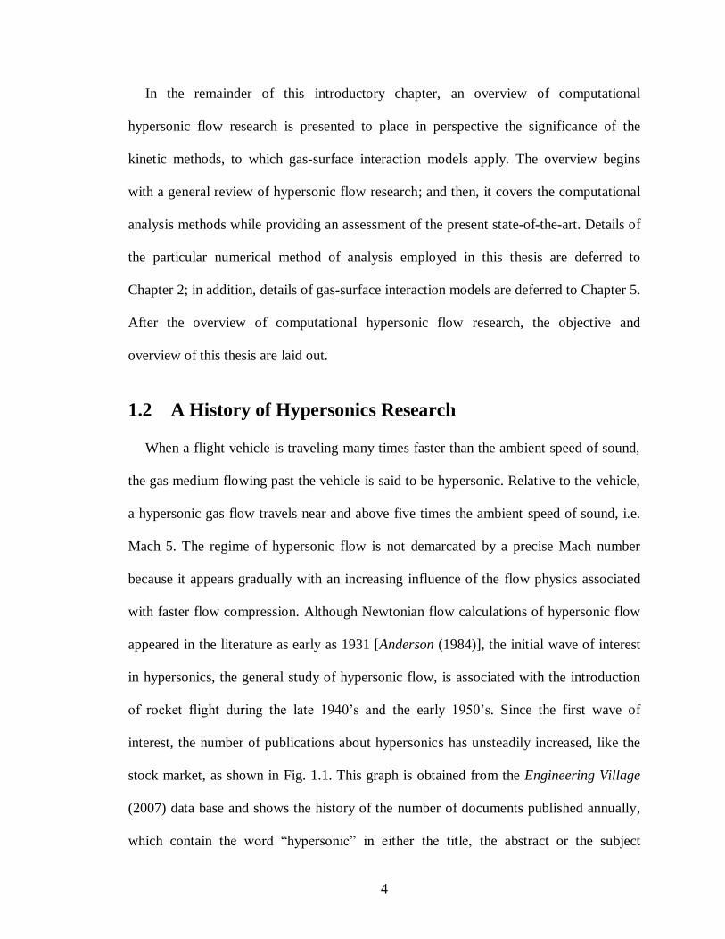
stock market, as shown in Fig. 1.1. This graph is obtained from the Engineering Village
(2007) data base and shows the history of the number of documents published annually,
which contain the word “hypersonic” in either the title, the abstract or the subject

5
description. The data base considers conference papers, journal papers, thesis reports and
books. Since 1948, the total number of such documents is 11,892. Although the data base
does not contain all engineering documents ever published, it does provide an adequate
statistical sample for representing the full population trends.
Figure 1.1 shows an increase in publicly published hypersonics research in the late
1950’s and early 1960’s. This increase can be attributed to the dawn of the space race
between the Soviet Union and the United States, which was instigated by the arrival of
space faring rocketry and emphasized 50 years ago by the first man made satellite,
Sputnik of the Soviet Union. The increase in publications continues until 1970, where the
number of publications hits a plateau. Then, a recession in hypersonics research occurs
Figure 1.1 History of documents containing
“hypersonic” in the title, abstract or
subject [Engineering Village (2007)]
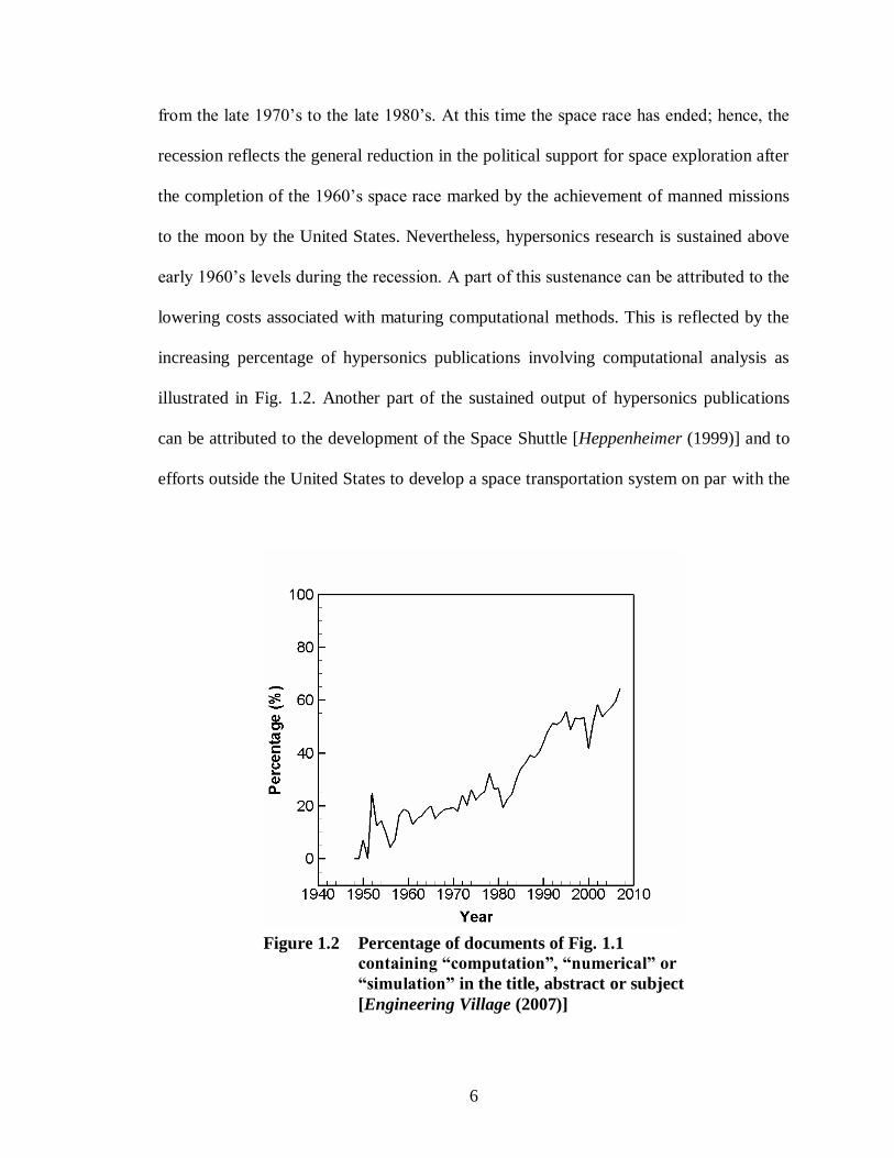
6
from the late 1970’s to the late 1980’s. At this time the space race has ended; hence, the
recession reflects the general reduction in the political support for space exploration after
the completion of the 1960’s space race marked by the achievement of manned missions
to the moon by the United States. Nevertheless, hypersonics research is sustained above
early 1960’s levels during the recession. A part of this sustenance can be attributed to the
lowering costs associated with maturing computational methods. This is reflected by the
increasing percentage of hypersonics publications involving computational analysis as
illustrated in Fig. 1.2. Another part of the sustained output of hypersonics publications
can be attributed to the development of the Space Shuttle [Heppenheimer (1999)] and to
efforts outside the United States to develop a space transportation system on par with the
Figure 1.2 Percentage of documents of Fig. 1.1
containing “computation”, “numerical” or
“simulation” in the title, abstract or subject
[Engineering Village (2007)]
7
Space Shuttle, namely, the French Hermes [Coue (2003)] and the Soviet Buran
[Pesavento (1995)]. The end of the recession in hypersonics research can be attributed to
the 1986 US state of the union address given by President Reagan, where he promoted
the development of a hypersonic cruise vehicle [Reagan (1986)] for defense and
commercial applications. This message evidently had a global impact, as the
development of the Hermes spaceplane, which had been on the drawing boards since the
late seventies by the French space agency, was revived in 1986 to be part of a European
space transportation system [Cazin (1989)]. In addition, Russia had responded with the
development of its own hypersonic cruiser [Poukhov (1993)]. This wave of hypersonics
research begins waning in the mid 1990’s. The reduction in hypersonics research can
again be attributed to loss in political interest, this time, due to failures in the ambitious
projects and escalations in their respective costs. Nonetheless, the output in hypersonics
documents never dips below late 1960’s levels. In the latter half of the 1990s, the
sustained research can be attributed mostly to further lowering of costs associated with
maturing computational capabilities, as reflected by the continuing rise in the percentage
of hypersonics publications involving computational analysis shown in Fig. 1.2. This
attribution is backed by the fact that the associated windtunnel and flight testing costs did
not have a lowering trend and the political climate did not foster ambitious hypersonics
developments. Further along the time line, Fig. 1.1 shows a third escalation in
hypersonics research occurring after the Columbia Orbiter disaster of 2003. This is
accompanied with a continuing rise in the percentage of papers involving computational
analysis, an increase of 10% every 10 years, illustrated in Fig. 1.2. If this trend continues,
then by 2020, 70% of publications about hypersonics will involve computational

8
analysis. Thus, the publications history reveals that the level of hypersonics research,
based on the number of publicly published papers on hypersonics, reflects the global
political climate, failures and advances in spaceflight programs, and the state-of-the-art in
research and development technologies. In particular, computational capabilities are seen
to play an increasing role in hypersonics research.
1.3 Computational Methods for Hypersonic Flow
The computational capabilities in hypersonics research are given by the existing state-
of-the-art in computer technology and in the computational methods. In this section, an
overview of computational methods in hypersonic flow analysis is given to place in
perspective the relevance of the kinetic methods.
1.3.1 Pre electronic digital computer methods
The earliest computational methods of hypersonic flow research were based on
approaches with limited applicability. These methods either drew upon existing theories,
by modifying them to suit hypersonic flow conditions, or on experimental data to form an
empirical formulation. They are of this nature because they were exploited during the
first wave of interest in hypersonic flow, which occurred before digital electronic
computing technology had come of age. These methods include, but are not limited to,
the Newtonian method, blast wave theory, inviscid compressible flow theory, laminar
boundary layer theory and empirical correlations. A review of these methods is given by
the books of Hayes and Probstein (1959) and (1966), Anderson (1989) and Rasmussen
(1994). Here they are only mentioned in passing in order to lay out the general
hypersonics research background. The Newtonian method, which is the earliest and most
9
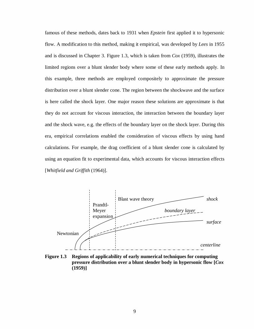
famous of these methods, dates back to 1931 when Epstein first applied it to hypersonic
flow. A modification to this method, making it empirical, was developed by Lees in 1955
and is discussed in Chapter 3. Figure 1.3, which is taken from Cox (1959), illustrates the
limited regions over a blunt slender body where some of these early methods apply. In
this example, three methods are employed compositely to approximate the pressure
distribution over a blunt slender cone. The region between the shockwave and the surface
is here called the shock layer. One major reason these solutions are approximate is that
they do not account for viscous interaction, the interaction between the boundary layer
and the shock wave, e.g. the effects of the boundary layer on the shock layer. During this
era, empirical correlations enabled the consideration of viscous effects by using hand
calculations. For example, the drag coefficient of a blunt slender cone is calculated by
using an equation fit to experimental data, which accounts for viscous interaction effects
[Whitfield and Griffith (1964)].
Blast wave theory shock
Prandtl-
Meyer boundary layer
expansion
surface
Newtonian
centerline
Figure 1.3 Regions of applicability of early numerical techniques for computing
pressure distribution over a blunt slender body in hypersonic flow [Cox
(1959)]

10
In order to examine heat transfer, the early hypersonic research subscribes to the
stagnation point heat transfer solution of laminar boundary layer theory [Fay and Riddell
(1958)]. Laminar boundary layer theory is also used to estimate the effects of chemical
reactions within the shock layer [Linen (1962)] on the aerothermodynamics of an
idealized flow geometry. In addition, correlation equations are developed to determine
stagnation point heat transfer to blunt bodies of revolution with a specified velocity and
nose radius [Detra et al. (1957)]. Correlation equations such as this enable rapid design
estimates. Finally, to model nonequilibrium effects, there are extensions to the
equilibrium models. For example, Freeman (1958) provides an addendum to Lighthill’s
ideal dissociating gas model in an effort to account for chemical nonequilibrium.
1.3.2 Continuum computational methods
To overcome the limitations of the early methods, the development of direct solutions
to the fundamental conservation equations of fluid flow is desired. This is made practical
with digital or transistorized computer hardware and an efficient programming language,
which did not arrive until the late 1950’s [Ceruzzi (2003)]. The maturing of the transistor
and the integrated circuit inevitably brought forth the development of high level
programming languages; the most popular, from this time, being FORTRAN, which has
descendant forms still widely used today. Prior to this time, numerical solutions to partial
differential equations were limited to basic mathematical forms, such as the Laplace
equation; however, it was then that the mathematical tools behind computational fluid
dynamics (CFD) were established by the pioneering efforts of various scientists. A
historical perspective on these efforts is presented by Anderson et al. (1984). What is
notable here is the relevance of computer technology in the development of CFD

11
solutions. For hypersonic flow problems, this development encompasses a spectrum of
flow conditions, which in terms of the advancing complexity ranges from inviscous
continuum to nonequilibrium rarefied conditions.
Regarding the continuum computational methods for hypersonic flow, accounts are
found in the books by Anderson (1989), Anderson et al. (1984) and Rasmussen (1994),
and the review paper by Cheng (1993). In brief, it is seen that the Navier-Stokes (NS)
equations provide the framework for most of the continuum analysis. In order to solve the
NS equations, various numerical methods are available. For a review of the numerical
methods refer to Hirsch (2007). Because of the complexity of the NS equations, various
simplified forms of the equations are developed. Relevant to hypersonic flow, these
include the Euler equations, the parabolized Navier-Stokes (PNS) equations and the
viscous shock layer (VSL) equations. The Euler equations provide estimations of shock
curvature and pressure distributions for hypersonic flow problems. They are suited for
code development; for example, Henderson and Menart (2006) used the Euler equations
to examine equilibrium air chemistry procedures for a Navier-Stokes code. When coupled
with boundary layer equations, the Euler equations provide suitable results for laminar
conditions with weak viscous interaction [Mundt (1992)]; these conditions are associated
with moderate to low altitude windward blunt body flows. The PNS and VSL equations
are more general and necessary for conditions with strong viscous interaction or fully
viscous shock layers. The PNS equations are suitable for shock layer flows where the
inviscid portion is primarily supersonic, for example, the windward flow field around
slender bodies. The VSL equations are applicable to shock layers with significant
12
subsonic flow, such as the windward flow against a blunt body. These simplified sets of
NS equations are not suitable for handling streamwise flow separation and turbulence.
In addition to the general problem of viscosity there is the related problem of
turbulence, which appears in a broad range of high Reynolds number applications. While
the NS equations are adequate for accounting for turbulence, using them directly to
calculate turbulence, which is known as direct numerical simulation (DNS), is intractable
for most practical applications; and thus, extensive modeling is employed. Turbulence
modeling is a broad topic which contains, as a sub-topic, simplifications to NS solutions.
For a general understanding of the subject, a host of text books are available, such as
Pope (2000). A recent review of engineering turbulence models for hypersonic flows is
provided by Roy and Blottner (2006). An example of turbulence in hypersonic flow is a
Mars entry space capsule analysis, presented by Brown (2002), which indicates that
transition to turbulence occurs at the shoulder of the space capsule under continuum
conditions.
The NS equations also provide the framework to model certain nonequilbrium
conditions. There are various general flow phenomena classified as nonequilibrium. One
major class is thermal nonequilibrium, which occurs when the translational, rotational
and vibrational temperatures are not all equal. Another class is chemical nonequilibrium,
which occurs when there is a finite rate of change in the chemical composition of the gas
flow. Chemical nonequilibrium in hypersonic flow is driven by various types of reactions
including dissociation, exchange, recombination and ionization reactions. In order to
extend the NS equations and their simplified forms for handling thermal and chemical
nonequilibrium flow, additional equations are added to the basic system of conservation

13
equations [Park (1990)]. For thermal nonequilibrium there is an additional energy
equation associated with each energy mode temperature. For chemical nonequilibrium,
there is an additional mass conservation equation associated with each distinct chemical
species undergoing a change in concentration.
1.3.3 Kinetic computational methods
Suborbital hypersonic flight vehicles, particularly near and above the Kármán line
defined in Section 1.1, experience conditions where the NS equations are erroneous in
major regions of the flow field surrounding the vehicles, mainly because of extremely
low gas density. In these regions, the dynamics of molecular motion need to be taken into
account; hence, the flow is said to encounter continuum breakdown. To accurately
describe a discrete gas, it is necessary to harness a molecular description of fluid
dynamics. Before proceeding, a few points on related terminology are made here. The
term “kinetic” is often used synonymously with “molecular”. These descriptions indicate
that intermolecular collisions or interactions are taken into account in some form. In
addition, because the description of relaxation to equilibrium is generally important when
describing fluid dynamics kinetically, the term “nonequilibrium” is also used
synonymously with “molecular”. Finally, for low gas density conditions, the application
of these terms: “kinetic”, “molecular” and “nonequilibrium” to gas flows are also used
interchangeably with the term “rarefied”.
There are a few classes of computational approaches for examining molecular gas
dynamics. One class is aimed at solving the Boltzmann equation, the standard governing
equation of kinetic theory [Cercignani (2000); Gombosi (1994); Vincenti and Kruger
(1965)]; for a historical perspective on kinetic theory see Gombosi (1994). In its general

14
form, the Boltzmann equation is a non-linear integro-differential equation in terms of a
function describing the distribution of molecules in position and velocity space. Hence,
the Boltzmann equation is solved numerically in practical applications. As early as 1955,
Nordsieck developed a Monte Carlo method to evaluate the collision integral of the
Boltzmann equation; this method was further developed by various researchers including
Yen (1984). According to Ivanov and Gimelshein (1998), newer methods have appeared
that preserve conservative variables by using special quadrature for the collision integral.
For example, in 1994 Rogier and Schneider published a solution method that uses a
finite-difference scheme to evaluate the collision integral and a finite element scheme to
evaluate the transport dynamics. This approach is classified as a discrete velocity model
of the Boltzmann equation; a solution method that has yet to fully mature [Cercignani
(2000)].
A second class of approaches to compute nonequilibrium gas flows involves solving
simplified forms of the Boltzmann equation, which are able to handle a greater extent of
nonequilibrium than the NS equations. Although the NS equations were developed before
the Boltzmann equation [White (1991); Gombosi (1994)], the NS equations are derivable
from the Boltzmann equation. This is performed by employing a truncated Chapman-
Enskog expansion of the velocity distribution function that has only a small deviation
from equilibrium [Vincenti and Kruger (1965)]. Consequently, the ability of the NS
equations to handle nonequilibrium flow is limited; however, other simplifications of the
Boltzmann equations exist that allow greater deviations from equilibrium. Simplified
forms that have appeared in aerospace applications include the Bhatnagar-Gross-Krook
(BGK) equation [Vincenti and Kruger (1965); Burt (2006)], the Burnett equations and

15
Grad’s moment equations [Cheng and Emanuel (1995); Chen et al. (2007)]. While these
equations involve solutions with less computational expense than the solution of the
Boltzmann equation, their computational expense is generally greater than solution of the
NS equations. In addition, their range of applicability is nevertheless limited and they
have yet to gain wide spread use.
A third class, called molecular dynamics, involves tracking every molecule of a
specified system by using the fundamental laws of physics. This approach was introduced
by Alder and Wainwright in 1958 and has since been substantially developed. The
molecular dynamics approach is employed for molecular scale simulations. When used
by itself, molecular dynamics is prohibitively expensive for vehicle aerothermodynamic
analysis; however, in relation to aerothermodynamics, it has found an auxiliary use. In
1999, Yamanishi et al. employed molecular dynamics for generating a gas-surface
interaction database for Monte Carlo simulation.
A fourth class involves kinematically tracking a representative system of molecules,
while using probability to select intermolecular collisions. This approach was not
developed from the Boltzmann equation; however, it uses the same physical principles
behind the Boltzmann equation [Bird (1994)]. In 1963, Bird introduced an early form of
the approach that eventually developed into what is now known as the direct simulation
Monte Carlo (DSMC) method [Bird (2001)]. The DSMC method has become the
standard approach to model flows with continuum breakdown at spatial scales relevant to
suborbital space flight aerothermodynamic analysis. Although the DSMC method has
been under development for over forty years, there are still many areas where
improvements can be made, from practical to fundamental theoretical considerations. It

16
forms the basis for the computational analysis in this thesis and is further discussed in
Chapter 2.
1.4 Objective and Overview
This thesis research focuses on the DSMC method for the analysis of rarefied
hypersonic flow aerothermodynamics relevant to the advancement of spaceflight. Several
aspects are examined, from the analysis of aerodynamic coefficients to an assessment of
gas-surface interaction models. The presentation of the research begins in Chapter 2 with
an introductory description of the DSMC method and the particular implementation
employed in this work, called MONACO. Then, a description is given of the grid-
generation procedures and post processing.
Having described the DSMC method and the associated simulation procedures, the
research analysis begins in Chapter 3 with the assessment of aerodynamics modeling
using data from rarefied hypersonic windtunnel tests of small scale entry vehicle models.
In this analysis, procedures to determine aerodynamic coefficients from MONACO
simulations are validated against certain experimental data and an independent DSMC
code.
In Chapter 4 the analysis continues with a sensitivity study of aerothermodynamics
predictions for the Apollo 6 capsule, at the 110 km altitude return trajectory point. This
involves the examination of inter-gas chemistry, a radiative equilibrium wall boundary
condition, and partial gas-surface accommodation. At this altitude it is found that changes
in the gas-surface thermal accommodation significantly affect the aerothermodynamics;
the addition of surface radiative equilibrium condition does not significantly affect the

17
aerothermodynamics; and the inclusion of chemistry does not significantly affect the
aerothermodynamics.
The conclusion to the sensitivity study motivates the detailed examination of gas-
surface interaction models presented in Chapter 5. This entails a review of existing
models and the analysis of two common models in use with the DSMC method: the
Maxwell model and the Cercignani, Lampis and Lord (CLL) model. The two models are
scrutinized with the help of relatively recent windtunnel test measurements of boundary
layer velocity profiles over a flat plate in rarefied hypersonic flow. The flow is analyzed
parametrically with various levels of gas-surface accommodation. The resulting effects
on velocity and temperature shock layer profiles and on surface friction and heating are
examined. Both models are found to yield similar results; however, the CLL model is
physically more realistic and is not significantly more expensive computationally. After
analyzing the gas-surface interaction models, the effects of seeded iodine in the
windtunnel tests are examined. These effects are found to be insignificant. Finally, the
extent of translational and rotational nonequilibrium within the boundary layer of the flat
plate is examined by molecular velocity statistics and distribution shapes, and profiles of
translational and rotational temperature. Significant thermal nonequilibrium is found near
the surface and near the leading edge of the flat plate.
After Chapter 5, appears the thesis conclusion in Chapter 6. Here the important results
and conclusions throughout the thesis are summarized. Finally, areas of further research
prompted by this thesis are suggested.
18
CHAPTER II
GENERAL SIMULATION PROCEDURES
2.1 Overview of the DSMC Method
The direct simulation Monte Carlo (DSMC) method was first developed and applied
by Bird in 1963. It has recently been surveyed by Oran et al. (1998) and by Bird (2001)
himself. It is a computational simulation method grounded in kinetic theory and
stochastic processes. It involves kinematically tracking a representative system of
molecules, while using probability to select intermolecular collisions and to process
boundary conditions. Thus, it is suitable for describing dilute gas flows. A gas is dilute
when the mean molecular spacing spacing is at least an order of magnitude greater than the
characteristic molecular diameter diameter. In a dilute gas, the molecular motions are not
significantly affected by intermolecular field forces and collisions between two molecules
are quickly forgotten by each molecule. This condition results in molecular chaos, a
fundamental assumption behind the Boltzmann equation and the DSMC method. The
condition of molecular chaos states that the probability of finding two molecules at the
same position and velocity is equivalent to the product of each molecule’s probability of
being found in that position and velocity [Bird (1994)]. In DSMC, this condition allows
the treatment of collisions independent of molecular motions within suitable intervals of

19
space and time; namely, the computational cell size s must be less than the local mean-
free-path distance traveled by molecules between successive collisions and the
reference time step t must be less than the local mean collision time , the mean time of
flight spent by molecules between successive collisions. Note that these criteria depend
on the knowledge of the local mean values, which vary slightly in a steady state due to
the statistical nature of the simulation. In regions of large macroscopic gradients, Bird
(1994) generally recommends s < / 3 and t << .
The DSMC method tracks a representative system of simulation molecules through a
computational domain while simulating collisions stochastically. The system is merely
representative because of the prohibitive cost of performing a simulation with the large
number of molecules in a real situation. A typical computer workstation’s central
processing unit (CPU), such as a 1.5 GHz class CPU, with 1 gigabyte (GB) of random
access memory (RAM), can efficiently process a DSMC simulation with up to about
3106 particles. Even at the typical altitude of the International Space Station, 385 km
[Bond (2002)], the number density of the atmosphere is on the order of 1014
molecules /
m3
, according to the 1976 United States (US) Standard Atmosphere table [Lide (2007)].
At the edge of the atmosphere, ~100 km altitude, where the DSMC method is commonly
applied for spacecraft aerothermodynamic analysis, the number density is five orders of
magnitude greater at ~1019
m–3
. It is clear that we cannot process more than a very small
fraction of the molecules present.
During each time step, all particles are translated according to rectilinear kinematics,
then certain particles are probabilistically selected for collision to match the correct
collision frequency according to kinetic theory. Post-collision velocities are determined

20
from conservation of energy and momentum and the assumption of isotropic scattering.
The intermolecular collisions and associated molecular energy exchange are processed
with special subroutines in a DSMC code. Optionally, other subroutines are used to
manage chemical reactions, ionization and radiation. Ivanov and Gimelshein (1998)
provide a review of physical models used in DSMC relevant to rarefied hypersonics.
Here a brief overview on the topics relevant to this thesis is presented. The intermolecular
collisions are modeled using simplified intermolecular field potentials in order to
maintain feasible computational expense. Various models have been developed, each
having advantages and disadvantages; the best use of a particular model being application
dependent. For computing molecular energy exchange, among translational, rotational
and vibrational modes, energy exchange probability models are used. Most of these
models are based on the Larsen-Borgnakke (LB) phenomenological model [Borgnakke
and Larsen (1975)]. For rotational energy exchange, continuous and quantized energy
spectrum LB models are available. The quantum or discrete rotational energy models are
particularly valuable for low temperature simulations. For vibrational energy exchange,
discrete energy models are necessary to provide accurate and physically realistic results.
The chemical reaction procedures are based on collision theory from physical chemistry.
The original procedures [Bird (1979)] used a reaction probability that depended only on
the total collision energy (TCE) and is called the TCE model. A modification to these
procedures considers coupled vibration-dissociation and called the vibrationally favored
dissociation (VFD) model [Haas and Boyd (1992)]. For an overview on the effects of
ionization and thermal radiation in the gas flow, see for example, Ivanov and Gimelshein
(1998).
21
At the domain boundaries are inflow, outflow, symmetry and wall surface conditions
that regulate the transport of molecules into and out of the simulation domain. At the
inflow boundaries, Maxwellian distributions at the local boundary temperature and
velocity are typically employed to insert the molecules into the simulation domain. At the
outflow boundaries, a vacuum or background pressure condition can be specified to
handle the removal of molecules. The symmetry boundaries assume a mirror image on
the other side, thus, they reflect molecules specularly without changing their kinetic and
internal energy. Finally, surface boundary conditions require specialized routines to
model the gas-surface interactions, and optionally, gas-surface catalysis, surface radiation
heat transfer and surface conduction heat transfer.
The ratio of mean-free-path to characteristic length l is called the Knudsen number
and is used to define flow regimes and to gauge for continuum breakdown. When l is a
characteristic dimension of a flight vehicle, such as the body length, the Knudsen number
describes the overall vehicle flight condition and is called the global Knudsen number
Kn. The global Knudsen number provides definitions for overall flow conditions as
follows: continuum Kn < 10–4
, transitional rarefied 10–4
< Kn < 10–1
, rarefied 10–1
< Kn <
10 and collisionless Kn > 10. These definitions are indicative of the majority of the gas
flow behavior and have pragmatic utility in setting up flow simulations. DSMC can
describe gas flows throughout the entire spectrum of global Knudsen number, provided
that the flows are dilute. However, DSMC is best suited for the transitional and rarefied
flow conditions. These are conditions the Navier-Stokes (NS) equations cannot simulate
because of continuum breakdown and are the conditions of primary concern in this thesis.
For the continuum regime, DSMC is inordinately expensive and the NS equations are
22
quite adequate. For the free molecular flow regime, the collisionless Boltzmann equation
provides more efficient results for simple geometries. When l is the length scale of a
macroscopic gradient, the Knudsen number describes the local flow condition and is
suitable for gauging continuum breakdown. The gradient length local Knudsen number is
used to partition computational domains in simulations using continuum and kinetic
methods in separate regions. For details on using gradient length local Knudsen numbers
to gauge continuum breakdown and apply them to hybrid computational methods refer to
Wang and Boyd (2003) and Schwartzentruber et al. (2007).
2.2 Description of the MONACO DSMC Code
This study employs a general, cell-based implementation of the DSMC method called
MONACO [Dietrich and Boyd (1996)]. The name is not an acronym; rather, it serves as a
reminder of a mathematical concept that it employs, Monte Carlo simulation. Since its
inception, this particular code has been developed by a number of researchers including
Kannenberg (1995), Sun (2003), Wang (2004) and Burt (2006). In the respective
references, they provide additional descriptions of the DSMC method and MONACO.
These researchers implemented the code for a spectrum of applications including rocket
plume, micro scale airfoil and hypersonic windtunnel test analysis, and the development
of hybrid continuum and particle methods. In this study, the code is employed to simulate
space capsule reentry and rarefied hypersonic windtunnel tests. MONACO is written in C
[Deitel and Deitel (2001); Kernighan and Ritchie (1988)] and can be executed on serial or
parallel computer systems. The parallel procedures are encoded with the Message Passing
Interface (MPI) [Quinn (2004)]. For defining the computational domain, MONACO
employs structured or unstructured grids, with two or three spatial dimensions in National

23
Grid Project (NGP) format [Thompson (1992)]. Additionally, it provides the option of
running two or three dimensional flow simulations, or axisymmetric flow simulations,
with the appropriate grid type.
MONACO provides the option of using various procedures for handling the molecular
physics, which deal with inter-gas collisions and chemistry, and gas-surface interactions.
For gaseous intermolecular collisions, a near-field molecular potential model, described
by a molecular shape, regulates the collision dynamics. Currently, the code gives the
option of using either the variable hard sphere (VHS) model [Bird (1981)] or the variable
soft sphere (VSS) model [Koura (1992)]. For rotational energy exchange, it uses the
variable rotational energy exchange probability model, developed by Boyd (1990). For
vibrational energy exchange it uses the variable vibrational energy exchange probability
model, developed by Vijayakumar et al. (1999). The variability of the vibrational energy
exchange model is optional, so that simulations can exclude it when it is known that the
flow will not be vibrationally activated. MONACO also provides the option of employing
chemical reaction procedures, regulated by the TCE or the VFD models, described in the
previous section. For the gas-surface interactions, MONACO uses by default the
Maxwell model and an isothermal wall temperature distribution.
For part of this thesis study, the wall temperature condition is modified to model a
radiative equilibrium wall surface and the accommodation coefficient in Maxwell’s gas-
surface interaction model is divided among the translational, rotational and vibrational
energy modes. A description of these modifications is given in Chapter 4. This thesis
research also added the option of using the Cercignani, Lampis and Lord (CLL) gas-
surface interaction model in lieu of the Maxwell model. The theoretical principles of both

24
gas-surface interaction models and their implementation into MONACO are presented in
Chapter 5. Finally, the research motivated the addition of procedures to extract
probability distributions and associated statistics of velocity at requested points in space
or of reflected velocity at requested points on a solid surface, for each gas species
involved in the simulation.
2.3 General DSMC Grid Generation Procedure
As with continuum CFD, the generation of the computational grid for DSMC in
general plays a major part of the simulation procedure. The difficulty arises in optimizing
the grid to minimize simulation expense while maintaining a grid that will result in an
accurate solution. The optimization is desired for large simulations. It involves
minimizing domain size and optimizing cell density. The former criterion is bypassed
when the size of the domain is predefined by the problem, such as in certain internal flow
problems. When the domain size is not predefined, a suitable estimate can be made
through physical intuition about the flow behavior, consideration to any symmetry in the
problem and consideration to the goal of the simulation. The estimate should be made
larger than expected in order to contain the relevant flow phenomena, such as a diffuse
bow shock about an entry vehicle, so that a well informed decision can be made about
reducing the domain size. In the case of the diffuse bow shock, the freestream region
need only be large enough to accurately generate the shock; the rule of thumb is to have
at least five cells of freestream upstream of the known location of the beginning of the
diffuse shock.
For optimizing the cell density in DSMC, the grid cells are distributed so that the
spatial constraint, s < , previously described, is met in the limit as s approaches ;

25
essentially by setting s throughout the computational domain. Because is not
usually known throughout the flow field, it is estimated in order to generate the initial
grid. Without additional information, a characteristic inflow mean-free-path c, such as
the freestream mean-free-path, provides a starting point. If the flow is known to expand
in the simulation domain, then the cell sizes in the expansion region could be made larger
than c in order to reduce computational expense for the initial simulation run. Otherwise,
a uniform distribution of cells with s c provides an initial grid. The mean-free-path
distribution of the initial simulation then provides the information to generate a grid with
an optimum cell density. Usually, the second grid, called the adapted grid, provides a
sufficiently efficient and accurate simulation for engineering analysis. The process of
redistributing or adapting cells so that their sizes are similar to the local mean-free-path
can be done automatically through a specialized computer code. However, when such a
code is not available, the adaptation can be done manually with a reasonable success.
The entire process of optimizing the grid for minimal simulation expense can be
automated in theory, however, at a significant cost: it requires integrating grid generation
procedures into the DSMC code and adding specialized logic for domain size reduction.
Integrated grid generation is difficult to develop to the same level of flexibility and
efficiency as existing grid generation software, which have extensively optimized
procedures and are able to handle automatic cell density adaptation to a given simulation
output file [Owen (2007); Ollivier (2005)]. Full automation is difficult and unnecessary
for single simulation cases needing only one iteration of grid adaptation; however, for
studies involving: several slightly distinct simulations, complex steady flow problems
requiring multiple iterations of adaptation or unsteady flow problems, automation of at

26
least the adaptation of cells merits pursuit. In this case, the problem of redistributing cells
with optimum smoothness in an arbitrary domain can be avoided by limiting grid
modifications to the division or synthesis of existing cells. This is pursued, for example
by Wu et al. (2001). In continuum CFD, the grid optimization problem is distinct and has
been given significantly more attention.
In this study, the simulation domains are adapted manually. Three dimensional grids
are generated for the simulations studied in Chapters 3 and 4, and two dimensional grids
are generated for the simulations analyzed in Chapter 5. For generating these grids,
commercial software is employed because it provides consistent and efficient
convergence. The particular program employed is HyperMesh (2004) as recommended
by a research colleague [Cai (2005)].
To provide an example of grid adaptation, the grid generation process for the seeded
iodine simulation, discussed in Chapter 5, is outlined here. This simulation involves the
near-field rarefied hypersonic flow over a flat plate windtunnel test model. It has a
specified inflow location from measured data, 2 mm upstream of a flat plate leading
edge; however, the inflow height and the downstream domain size are undetermined. The
initial simulation uses the domain dimensions displayed in Fig. 6 of the windtunnel test
paper by Cecil and McDaniel (2005). This domain is divided into rectangular cells with
sides s equal to the average inflow mean-free-path c = N2, , avg of the nitrogen: s =
0.1 mm N2, , avg , as illustrated in Fig. 2.1 (a). This grid is comprised of 35,850 cells
and is more than adequate for simulations which assume a pure nitrogen flow. However,
for the simulation that includes the seeded iodine, the grid needs to be refined because the

27
(a) Initial Grid
(b) Close-up of Adapted Grid
Figure 2.1 Computational grid generation for seeded iodine simulation
28
iodine mean-free-path is an order of magnitude smaller than the nitrogen mean-free-path.
For the refined grid it is estimated that the number of simulation molecules is about 200
million. Hence, the domain size is reduced in order to maintain a reasonable
computational expense. The simulation expense of the reduced domain is listed in Table
5.5 of Chapter 5. A mixed set of triangular and quadrilateral cells is used because it
results in fewer cells and a smoother cell distribution. The mean-free-path adaptation is
performed manually by dividing the domain into several sub-regions and defining the cell
densities at the boundaries of each of these sub-regions. Figure 2.1 (b) illustrates a
portion of the adapted grid. The entire grid has too many cells to distinguish their
distribution within the page margins; hence, a close-up of the adapted grid is shown. The
close-up shows a few sub-regions with cell densities matching at their boundaries. The
sub-region containing the diffuse oblique shock has the greatest cell density because that
is where the iodine mean-free-path is smallest. Behind the shock the flow expands and
the associated the computational cell density is consequently lower.
2.4 Overview on Post Processing
A DSMC simulation begins with a transient period from the initial insertion of
simulation molecules into the simulation domain. Eventually, for a steady state
simulation, the collisional and other physical processes arrive at a statistical steady state.
Thereafter, molecular properties are sampled in each cell at specified intervals of time
steps and the running average or summation of each sampled property is monitored.
When the uncertainties in the running averages are within satisfactory limits, the
simulation is terminated. The MONACO DSMC code stores the cell averaged molecular

29
properties in an unformatted binary file called MCsample.unf. This file is converted into
Tecplot (2004) format with the OXFORD post-processing program.
OXFORD provides the option of examining several of the field and surface properties.
Some of the field properties are presented at various places throughout this thesis report.
These include the mean-free-path, the translational, rotational and vibrational
temperatures, the number density and the Mach number. To provide an example of how
the field properties are extracted the equations for the translational temperature are
presented. The translational temperature is computed by:
, , ,
1
3tra tra x tra y tra zT T T T (2.1)
where each component translational temperature is obtained using
2
,
,
12
2s s i s
stra i
u
MW X
TR
(2.2)
where Ru is the universal gas constant and the summation occurs over all species s. MWs,
Xs and 2
,i s represent the species molecular weight, mole fraction and mean square
random molecular speed along direction i, respectively. Each mean square random
molecular speed is determined by the identity
2 2 2
, , ,i s i s i s (2.3)
The set of molecular properties in each computational cell stored in MCsample.unf,
includes , , ,r t i s
t r
and 2
,i s . , , ,r t i s
t r
represents the summation over all particles r
and samples t at a particular computational cell of the species absolute molecular speed
along coordinate direction i. This provides the information to extract 2
,i s with the aid of

30
the relation:
, , ,
,
r t i s
t ri s
sample pN N
(2.4)
where Nsample is the total number of samples taken at a particular cell and Np is the mean
number of simulation molecules in that cell during steady state.
Surface properties that appear in this thesis report, directly or indirectly, are the
pressure p, the shear stresses x, y and z, and the Stanton number St. The pressure and
shear stresses are used to compute the aerodynamic coefficients of lift, drag and pitching
moment: CL, CD and CM, respectively. A further description on the calculation of the
aerodynamic coefficients is given in Chapter 3. To provide an example of how the
surface properties are extracted, the equations for the Stanton number are presented. The
Stanton number is computed by
31
2
qSt
V
(2.5)
where and V are the freestream density and speed, and q is the surface heat flux. The
heat flux is determined by
,
p
s p s
s A face
Wq E W
tN A
(2.6)
where sE and Wp,s are the species mean total energy transfer and particle weights,
respectively. The set of molecular properties at each computational cell stored in
MCsample.unf also includes sE . Wp, t, NA and Aface are the global particle weight,
global time step, Avogadro’s number and the wall surface cell face area, respectively. In
the simulations presented in this thesis, species particle weights are used only for the
iodine simulation.

31
CHAPTER III
ASSESSMENT OF AERODYNAMICS MODELING
AND WINDTUNNEL DATA
3.1 Background and Relevance
In the mid to late 1960’s, the Apollo program motivated hypersonic windtunnel test
studies of centimeter scale models in order to improve our knowledge of spacecraft
reentry aerothermodyamics. Some of these windtunnel studies were performed at the
Arnold Engineering Development Center (AEDC), Tennessee, in the von Karman Gas
Dynamics Facility (VKF) and involved a low density, hypersonic, continuous-flow, arc-
heated, and ejector-pumped windtunnel called VKF Tunnel L. One of these studies,
executed by Boylan and Potter (1967), tested a handful of simple vehicle shapes, and
compared the resulting windtunnel data with modified Newtonian and free molecular
flow analyses. Because of the simplicity of the vehicle models and the adequacy of the
documentation, this windtunnel test study is selected for numerical simulation in order to
develop three-dimensional aerodynamic post-processing procedures. The aerodynamic
procedures are validated by reproducing the modified Newtonian and free molecular flow
results. Subsequently, the aerodynamic procedures are applied to DSMC results, and the
DSMC aerodynamic results are compared with the windtunnel results. In addition,
32
similar numerical simulations are made of the VKF Tunnel L windtunnel tests of the
Apollo Command Module [Boylan and Griffith (1968)]. These simulations provide a
unique assessment that uses aerodynamic analysis within rarefied hypersonic flow
conditions of the MONACO DSMC code.
In this chapter, the computer aerodynamic simulation study of the AEDC windtunnel
tests described above are presented. First, a description is given of the Newtonian and
free molecular flow analyses. Second, the three-dimensional aerodynamic analysis is
formulated. Third, three-dimensional simulations of the blunted-cone model are
presented. Fourth, three-dimensional simulations of the Apollo command module model
are presented. Fifth, axisymmetric simulations are presented to help explain the
disagreement between the Apollo windtunnel test results and the DSMC results. Finally,
the aerodynamic assessment is summarized and conclusions are formulated about the
numerical simulations and the windtunnel tests.
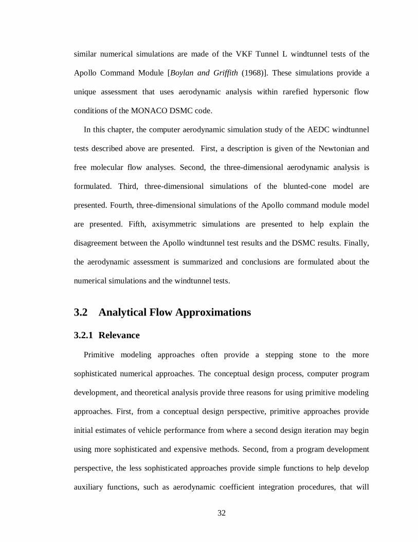
3.2 Analytical Flow Approximations
3.2.1 Relevance
Primitive modeling approaches often provide a stepping stone to the more
sophisticated numerical approaches. The conceptual design process, computer program
development, and theoretical analysis provide three reasons for using primitive modeling
approaches. First, from a conceptual design perspective, primitive approaches provide
initial estimates of vehicle performance from where a second design iteration may begin
using more sophisticated and expensive methods. Second, from a program development
perspective, the less sophisticated approaches provide simple functions to help develop
auxiliary functions, such as aerodynamic coefficient integration procedures, that will

33
eventually be used with more complicated procedures. Third, from a theoretical analysis
perspective, the less sophisticated theory often helps identify physical or numerical
phenomena and their effects.
In the following sections, the modified Newtonian and free molecular flow primitive
modeling approaches are described. They help develop procedures to compute
aerodynamic properties from DSMC analysis of the windtunnel tests. The aerodynamic
post-processing procedures are developed to expand our ability to evaluate modifications
and additions of physical models to the MONACO DSMC code.
3.2.2 Modified Newtonian flow
Numerical models can be selected for gas dynamic simulation based on freestream
speed. The AEDC windtunnel tests involved gas flow traveling at thousands of meters-
per-second with respect to the vehicle. A Newtonian model for solids immersed in a gas
flow is valid for inexpensive analysis of hypervelocity gases such as in the AEDC
windtunnel tests. The Newtonian model can be used with a flat panel surface
approximation to provide a simple numerical calculation to estimate the vehicle
aerodynamic properties. The details on this approach are described in this section.
Over three centuries ago, Isaac Newton made propositions to determine the pressure of
simple shapes, such as spheres, submerged in a steady uniform stream of a “rare
medium” [Anderson (1989); Cajori (1934); Chandrasekhar (1995)]. Incidentally, the
involved mechanics provide a rough estimation of vehicle aerodynamic properties in
hypersonic flow. In Newton’s model, the flow is comprised of rectilinear streams of
particles. The particles are assumed to lose all their normal momentum upon striking the
vehicle surface and then move tangential to the surface. Application of Newtonian
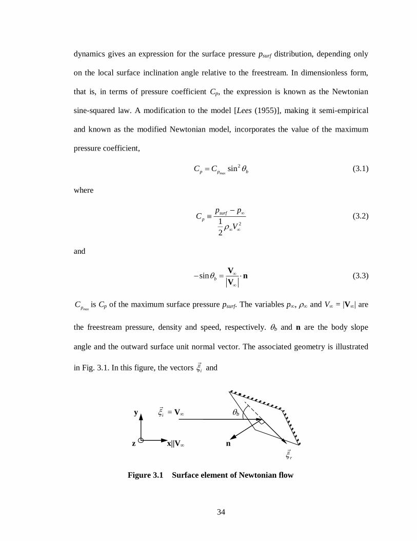
34
dynamics gives an expression for the surface pressure psurf distribution, depending only
on the local surface inclination angle relative to the freestream. In dimensionless form,
that is, in terms of pressure coefficient Cp, the expression is known as the Newtonian
sine-squared law. A modification to the model [Lees (1955)], making it semi-empirical
and known as the modified Newtonian model, incorporates the value of the maximum
pressure coefficient,
2sinmaxp p bC C (3.1)
where
21
2
surf
p
p pC
V
(3.2)
and
sin b
V
nV
(3.3)
maxpC is Cp of the maximum surface pressure psurf. The variables p, and V = |V| are
the freestream pressure, density and speed, respectively. b and n are the body slope
angle and the outward surface unit normal vector. The associated geometry is illustrated
in Fig. 3.1. In this figure, the vectors i
and
y i
= V b
z x||V n
r
Figure 3.1 Surface element of Newtonian flow

35
r
represent the incident and reflected molecular velocities. i
, r
and n lie in the same
plane. Newtonian theory assumes the incident molecular velocity i
equals the
freestream bulk velocity V. When 180 < b < 360, the surface pressure is set to the
freestream pressure, viz. Cp = 0. This flow model, with a good estimate of maxpC , can
provide an inexpensive estimate of hypersonic transitional flow aerodynamics for
configurations where pressure dominates over shear stress.
3.2.3 Free molecular flow
When the global Knudsen number (Kn = / l) is greater than roughly 10, the
freestream mean-free-path traveled by ambient molecules is much greater than the
characteristic length l of the vehicle and collisions between molecules within a few
characteristic lengths l from the vehicle become so few that the gas can be considered
collisionless. The motion of a collisionless gas is called a free molecule or a free
molecular flow. Properties of free molecular flow can be accurately computed by using
free molecular flow analysis [Gombosi (1994)]. Free molecular flow analysis is suitable,
for example, for calculating spacecraft drag above ~132 km where Kn > 10 for l = 1 m,
according to the 1976 US Standard Atmosphere [Lide (2007)]. However, in this study
free molecular flow analysis is not included to provide accurate results or even
conceptual design estimations; rather, it is included to provide physical insight and to
serve as an aid in the computer program development for the calculation of suborbital
flight aerodynamics, in particular, atmospheric entry aerodynamics. The flow properties
of interest in entry vehicle analysis are those that affect the vehicle’s performance. These

36
include the pressure, shear stress and heat flux. Detailed knowledge of these flow
properties enables the determination of the entry vehicle aerodynamic properties.
In the classic free molecular flow theory [Schaaf and Chambré (1961)], the vehicle is
assumed to be immersed in an infinite domain of a collisionless gas having a Maxwellian
velocity distribution appropriate to its temperature. Because molecules approaching the
vehicle surface do not collide with reflected molecules, the freestream molecules receive
no warning about the approaching vehicle and collide with its surface with the freestream
molecular velocity. During collision, the molecules accommodate kinetically and
thermally to the vehicle surface in a full or partial manner. When they are fully
accommodated, they reflect diffusely with a Maxwellian velocity distribution. The degree
of kinetic gas-surface accommodation in free molecular flow analysis is governed by the
tangential and normal momentum accommodation coefficients, t and n, respectively,
where t = n = 0 indicates no accommodation and specular reflection, and t = n = 1
indicates full accommodation and diffuse reflection.
The free molecular flow model is amenable to the derivation of expressions for
aerodynamic surface properties. Consider an infinitesimal flat polygonal (triangular,
rectangular, etc.) surface element, illustrated in Fig. 3.2, with a local coordinate system
i
V + i
n, t
y u
r
v
z x||V w
Figure 3.2 Surface element of free molecular flow

37
defined by the orthonormal set of vectors (u, v, w), where u is parallel to one side of the
element and the origin is at a corner. Vectors u and v lie in the same plane as the surface
element. The incident molecular velocity i
is the sum of the ambient bulk velocity V
and the incident random molecular velocity i
. The surface element’s polygonal shape is
specified here for simplicity of numerical application, wherein the elements approach
infinitesimal size only to a reasonable approximation. It can be shown that the
corresponding surface pressure psurf and shear stresses u and v are expressed by the
following equations [Sentman (1961)]:
2 2
2 2
2
2
12
22 1 1
2
x
x
w s
n w xsurf x
w s
nx n x x x
T wep q erf w s
T s s
ew w erf w s erf w s
ss
(3.4)
2 2
1xw s
u t x x x
eq u w erf w s
s
(3.5)
2 2
1xw s
v t x x x
eq v w erf w s
s
(3.6)
where ux, vx and wx are the components of u, v and w parallel to x. T and Tw are the
ambient flow temperature and the local surface temperature. q is the freestream dynamic
pressure and s is the molecular speed ratio:
21
2q V (3.7)
mp 2
Vs Ma
(3.8)

38
2mp Bk T m is the most probable molecular speed, where kB is the Boltzmann
constant, T is the local flow temperature, and m is the mean molecule mass of the
mixture. is the ratio of specific heats and Ma is the associated Mach number. In the
context of free molecular flow analysis, the freestream or ambient properties determine s.
Regarding the gas-surface accommodation, full gas-surface accommodation is assumed
for the free molecular flow analysis; that is, unity is assumed for the values of the
tangential and normal momentum accommodation coefficients, t = n = 1.
3.3 Aerodynamic Force Integration
Equations (3.4) through (3.6), provide two approaches for computing a vehicle’s
aerodynamic forces. The first approach involves setting up a conglomerate of elements
representing the surface of a vehicle. At a particular element, equations (3.4) through
(3.6), the local surface element area and a three-dimensional rotation of coordinate axes
result in the lift and drag forces on that surface element. The summation of these forces
over the conglomerate of elements yields the total lift and drag forces on the vehicle. A
similar procedure is used to compute the vehicle’s pitch, yaw and roll moments, with the
appropriate moment arms. These procedures enable the calculation of the aerodynamics
of a vehicle of arbitrary shape within a free molecular flow. The second approach
involves setting up the aerodynamic force integrals in terms of the pressure and shear
stresses, the appropriate infinitesimal area elements, and the integration limits
corresponding to the vehicle geometry. This approach is tractable for computing the
aerodynamic coefficients of simple shapes within a free molecular flow. This can be done
39
by beginning with the expression for the resultant pressure and shear force dF/dA on an
infinitesimal or differential surface element [Sentman (1961)]:
2 2
2 2
22 1
21
2
12
Vy
Vy
s
t Vx Fx Vz Fz n Vy Vy
n Fy
Vy
sn Fy wVy Vy
i
dF sq s erf s e
dA
erf s
Ts erf s e
T
(3.9)
where Vx , Vy and
Vz are the direction cosines between V and x, y and z,
respectively; and Fx , Fy and Fz are the direction cosines between dF and x, y and z.
The aerodynamic forces are then determined by resolving the resultant force into the drag
and lift directions, (dF/dA)D and (dF/dA)L, respectively, and setting up integrals for the
particular geometry and integrating either analytically or numerically. For example, the
general integral expressions for the drag and pitching moment about point () are written
below by Eqns. (3.9) and (3.10), respectively. In Eqn. (3.10), the functions armD and
surface
D
D
dFF dA
dA
(3.10)
surface
D LP
D L
dF dFM arm arm dA
dA dA
(3.11)
armL represent the variation of the moment arms referenced to point () and perpendicular
to the drag and lift directions, respectively, with element position.
In this study, the element summation approach is implemented in C code for
determining the aerodynamic forces from the pressure and shear stresses computed by
DSMC on an arbitrary vehicle shape represented by small surface elements. This
implementation of the summation approach is validated using the free molecular flow
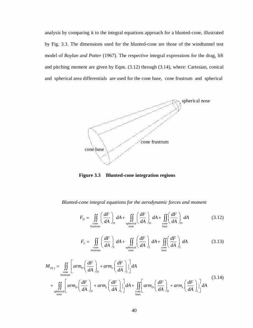
40
analysis by comparing it to the integral equations approach for a blunted-cone, illustrated
by Fig. 3.3. The dimensions used for the blunted-cone are those of the windtunnel test
model of Boylan and Potter (1967). The respective integral expressions for the drag, lift
and pitching moment are given by Eqns. (3.12) through (3.14), where: Cartesian, conical
and spherical area differentials are used for the cone base, cone frustrum and spherical
Blunted-cone integral equations for the aerodynamic forces and moment
cone spherical cone
frustrum nose base
D
D D D
dF dF dFF dA dA dA
dA dA dA
(3.12)
cone spherical cone
frustrum nose base
L
L L L
dF dF dFF dA dA dA
dA dA dA
(3.13)
cone
frustrum
spherical conenose base
D LP
D L
D L D L
D L D L
dF dFM arm arm dA
dA dA
dF dF dF dFarm arm dA arm arm dA
dA dA dA dA
(3.14)
Figure 3.3 Blunted-cone integration regions
cone base
cone frustrum
spherical nose

41
nose, respectively. For brevity, the equations are not expanded further. Comparisons are
made of the nondimensionalized forces and moment, that is, the force and moment
coefficients. For reference, the definitions of lift and drag coefficients and of the pitching
moment coefficient about point () are listed respectively by the following equations:
DD
ref
FC
q A
(3.15)
LL
ref
FC
q A
(3.16)
P
M
ref ref
MC
q A d
(3.17)
where the reference area is the area of the cone base, Aref = dref2 / 4, and the reference
length dref, is the diameter of the cone base. Comparisons are also made of the lift-to-drag
ratio: L/D FL / FD = CL / CD.
Equations (3.12) through (3.14) are integrated numerically with MathCad (1998) and
compared with the implementation of the summation approach applied to a flat panel
representation of the blunted-cone. The precise agreement between the two integration
procedures is demonstrated in Figs. 3.4 (a) and (b). To generate all the data shown in
these figures, the calculations on a 3 GHz personal computer take about 24 seconds by
the integral equations and about 100 seconds by the element summation. This indicates
that the integral equations approach is generally faster, although it is limited to simple
geometries.
Apart from validating the element summation approach, Figs. 3.4 (a) and (b) provide
information about the blunted-cone free molecular flow aerodynamics. The variations of
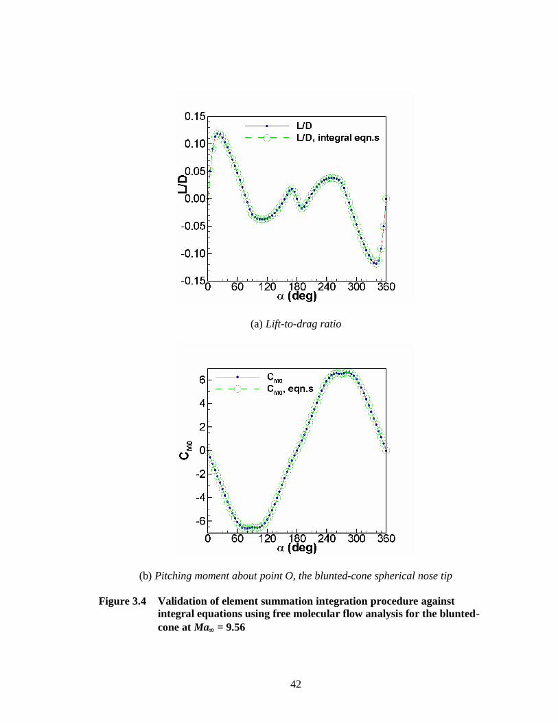
42
(a) Lift-to-drag ratio
(b) Pitching moment about point O, the blunted-cone spherical nose tip
Figure 3.4 Validation of element summation integration procedure against
integral equations using free molecular flow analysis for the blunted-
cone at Ma = 9.56

43
L/D and CMO as functions of angle-of-attack are governed by the vehicle shape. They are
odd functions about 180 because of the axisymmetry. The L/D variation is primarily
governed by the lift variation. The angle of maximum L/D, which is 20, is also the angle
of maximum lift. The L/D becomes negative between 75 and 80 because that is where
the blunted-cone begins exhibiting negative lift, which is related to its 9 half angle. The
L/D increases between 110 and 170 because that is where the cone base becomes
exposed to the freestream and produces increasing lift. The sinusoidal behavior of the
pitching moment variation can be attributed to the slenderness and symmetry of the
blunted-cone. The plateau regions of the CMO curve occur when the cone base becomes
exposed to the freestream; and thus, are due to counteracting moment components from
the cone base.
3.4 Blunted Cone Simulations
3.4.1 Flow conditions and geometry
Flow conditions and geometry for the blunted-cone windtunnel test [Boylan and
Potter (1967)] are shown in Table 3.1 and Fig. 3.5, respectively. These conditions include
the Reynolds number defined by Red = Vdref / , where is the freestream
viscosity. The value of Red is provided by the Boylan and Potter (1967) and reflects the
low viscosity of the transitional rarefied flow. The pitching moment for the 9 blunted-
cone is taken with respect to point O. More details of the cone’s geometry are given by
Boylan and Potter (1967). Because the windtunnel test model has a global Knudsen
number that is within the rarefied transitional flow regime, the DSMC method is suitable
for estimating the model’s aerodynamics. These conditions provide some of the starting

44
parameters for the DSMC calculations.
Three-dimensional computational domain boundaries for the DSMC simulations are
generated with Pro/ENGINEER (2004). They are then exported to HyperMesh (2004), a
grid generation program, which is used in this case to create an unstructured tetrahedral
mesh, with cell-sizes manually adapted to the local mean-free-path, according to the
DSMC constraint. Figure 3.6 is an image of the domain boundary surface mesh, with the
model at a 20 angle-of-attack. The symmetry of the blunted-cone geometry and the
assumed uniform inflow boundary requires simulation of only half of the domain. In this
study, three-dimensional simulations are made for the blunted-cone at 0, 10, 20 and 25
degrees angle-of-attack. A distinct mesh is generated for each angle-of-attack case, where
each mesh consists of roughly 560,000 tetrahedral cells. For the modified Newtonian and
free molecular flow calculations, only the vehicle surface grid is necessary. The surface
grids are extracted from the three-dimensional grids employed in the DSMC calculations,
and involves only about 1,900 cells.
Figure 3.5 Blunted-cone geometry
V
C L
O
CMO
dref
9
Table 3.1 Conditions of blunted-
cone windtunnel test
Property Value
dref 1.524102
m
Gas N2
T 143.5 K
Ma 10.15
Red 233
Tw 600 K
Kn 0.065
n 1.3231021
m–3
9.910–4
m
V 2478 m/s

45
3.4.2 Results and discussion
Figure 3.7 illustrates the general character of the flow field for the blunted-cone. The
freestream region is sufficiently large to capture the diffuse shock near the windtunnel
test model and the peak flow temperature is not sufficient to justify activation of nitrogen
dissociation procedures [Anderson (1989); Josyula (2001)].
The aerodynamic results of the DSMC simulations for the blunted-cone, with two
values of Maxwell’s accommodation coefficient aM, are compared with the simpler flow
models and the available windtunnel data. (Maxwell’s gas-surface interaction model as
implemented into the MONACO DSMC code is described in Chapter 5 where gas-
Figure 3.6 Domain boundary for simulation of blunted-cone at a 20
angle-of-attack

46
surface interaction models are reviewed and aM is defined.) Figure 3.8 (a) compares the
drag coefficient among the computer calculations and the windtunnel tests at various
angles-of-attack. In these figures, the DSMC calculations generally yield lift and drag
coefficients that lie somewhere between the values given by the modified Newtonian and
free molecular flow results. A major reason the modified Newtonian model predicts
lower drag is that it neglects shear stress. The free molecular flow model predicts higher
drag because it neglects intermolecular collisions. The modified Newtonian analysis for
the blunted-cone employed maxpC = 1.83, from Boylan and Potter (1967). The
Figure 3.7 Contour plot of translational temperature at symmetry
boundary of three-dimensional windtunnel test
simulation with blunted-cone at 20 angle-of-attack

47
(a) Drag Coefficient
(b) Lift Coefficient
Figure 3.8 Variation of blunted-cone drag and lift with angle-of-attack with the
modified Newtonian (MN) model, the free molecular flow (FMF)
model, DSMC at two values of gas-surface accommodation aM, and
windtunnel results from the AEDC VKF Tunnel L

48
disagreements between the simpler models and DSMC provide a measure on the effects
of the neglected phenomena in the simpler models. Figures 3.8 (a) and (b) indicate that
shear stress and intermolecular collisions play strong roles in the lift and drag integration,
with the drag affected more.
The variation of CD with given by the DSMC cases agree well with that of the
windtunnel data. The DSMC, with aM = 1, and the windtunnel data are 6.9, 8.7, 7.8 and
7.7% different from the windtunnel data at 0, 10, 20 and 25, angle-of-attack,
respectively. At 0 angle-of-attack, a reduction in the thermal accommodation coefficient
by 15% reduces the drag coefficient by 6%, from 0.82 to 0.77. Figure 3.8 (a) shows that
the reduction in accommodation uniformly affects the drag at all the angles-of-attack
considered. The reduction in drag due to a reduction in aM is a consequence of reduced
backscatter by the introduction of specular reflections in the Maxwell gas-surface
interaction model. This reduction moves the DSMC results slightly further from the
windtunnel drag data; thus, it indicates that full gas-surface accommodation is the more
accurate estimate between the two DSMC cases. Figure 3.8 (b) illustrates the
comparisons for the lift coefficient. The DSMC lift trend also agrees well with the
windtunnel data. The difference between the DSMC and windtunnel data is about 10% at
10, 20 and 25 angle-of-attack. At zero angle-of-attack, the lift coefficient is zero because
of the prescribed symmetry. There, the nonzero windtunnel data is probably due to
statistical scatter. The uncertainty of the windtunnel measurements is not reported by
Boylan and Potter (1967). The reduction in the gas-surface accommodation coefficient
does not significantly affect the lift coefficient.

49
(a) Lift-to-drag ratio
(b) Pitching moment about blunted-cone spherical nose tip
Figure 3.9 Variation of blunted-cone lift-to-drag ratio and pitching moment with
angle-of-attack with the modified Newtonian (MN) model, the free
molecular flow (FMF) model, DSMC at two values of gas-surface
accommodation aM, and windtunnel results from the AEDC VKF
Tunnel L
50
Figure 3.9 (a) illustrates the comparisons for the lift-to-drag ratio. Again, the DSMC
data lie well within the modified Newtonian and the free molecular flow data. The
DSMC lift-to-drag ratio is not significantly affected by the 15% reduction in gas-surface
accommodation, and there is no significant difference between the DSMC and
windtunnel data. The agreement between the DSMC and windtunnel data of the lift-to-
drag ratio is closer than that of the individual lift and drag comparisons, c. f. Figs. 3.8 (a)
and (b). Taking the ratio of the lift and drag seems to cancel out some of the error given
by the individual lift and drag comparisons; hence, separate lift and drag comparisons
provide closer scrutiny of the DSMC data evaluated relative to the windtunnel data.
Figure 3.9 (b) illustrates the comparisons for the pitching moment. Once again, the
DSMC results lie between the simpler model results. The reduction in gas-surface
accommodation coefficient does not incur any significant effect on the DSMC results,
and the DSMC results agree well with the windtunnel results. At zero degree angle-of-
attack the pitching moment is zero because of the prescribed symmetry. From 10 to 25
angle-of-attack, the agreement between the DSMC and windtunnel pitching moment
results improve with increasing angle-of-attack. The Percentage differences between the
DSMC and windtunnel pitching moment are 11, 5, and 2% for = 10, 20 and 25,
respectively. However, the small improvements are likely within the uncertainty of the
windtunnel test data, again not reported by Boylan and Potter (1967).

51
3.5 Apollo Command Module Simulations
3.5.1 Flow conditions and geometry
Flow conditions and geometry for the Apollo Command Module (ACM) windtunnel
test [Boylan and Griffith (1968)] are shown in Table 3.2 and Fig. 3.10, respectively.
Figure 3.10 shows the location of the center-of-gravity with respect to the windward heat-
shield apex and defines the angle-of-attack with respect to the leeward vehicle axis of
symmetry. The pitching moment for the ACM is taken relative to the center-of-gravity.
Further details of the ACM geometry are given by Boylan and Griffith (1968).
The flow conditions are similar to the blunted-cone windtunnel test. The Knudsen
number is well into the transitional rarefied flow regime, so the DSMC method again
provides a suitable approach for analysis. The procedures for setting up the numerical
simulations are similar to those described for the blunted-cone simulations, Section 3.4.1.
Figure 3.11 is an image of the domain boundary surface mesh, with the ACM windtunnel
model at an angle-of-attack of 150. Three-dimensional windtunnel test simulations are
C L
Figure 3.10 ACM geometry
CMcg
V
x
e
cg
dref
Table 3.2 Conditions for the ACM
windtunnel test
Property Value
dref 1.524102
m
Gas N2
T 142.2 K
Ma 10.20
Red 230
Tw 300 K
Kn 0.067
n 1.2801021
m–3
0.001 m
V 2479 m/s

52
made for the ACM at angles-of-attack of 180, 170, 160, 150 and 140, where a distinct
mesh is generated for each angle-of-attack. Each of these meshes has about 740,000 cells
or 32% more cells than the blunted-cone simulations. The larger number of cells is due to
the larger compression region, which is due to the broader size of the model’s front end.
Compression regions or regions of higher density within the shock layer require more
cells in order to handle associated smaller mean-free-paths. The ACM surface meshes,
Figure 3.11 Domain boundary for simulation of ACM at a 150 angle-of-
attack

53
employed for the modified Newtonian and free molecular flow calculations, and
extracted from the three-dimensional meshes, involve about 8,960 cells.
3.5.2 Results and discussion
The analysis of the ACM windtunnel simulations is similar to the analysis of the
blunted-cone simulations. However, for the ACM DSMC calculations only full gas-
surface accommodation is employed since a reduction of 15% accommodation is not
expected to affect the results significantly. Figure 3.12 illustrates the general character of
Figure 3.12 Contour plot of translational temperature at symmetry
boundary of three-dimensional windtunnel test
simulation with ACM at 150 angle-of-attack

54
the flow field about the ACM. The freestream region is sufficiently large to capture the
diffuse shock near the vehicle and the peak flow temperature is again not sufficiently
large to justify activating chemical reaction procedures.
Figures 3.13 and 3.14 compare windtunnel and simulation data of CL, CD, L/D and
CMcg at various angles-of-attack for the ACM. In these figures, the DSMC calculations
generally yield lift and drag coefficients that lie somewhere between the values given by
the modified Newtonian and free molecular flow results. The modified Newtonian
analysis employed maxpC = 1.89, obtained from the DSMC analysis. The windtunnel CD,
CL and L/D were extracted from separate plots in Griffith and Boylan (1968). For the
ACM, a second set of DSMC results are plotted. These results are provided by Dr. James
Moss (private communication, Dec. 2005) from NASA Langley Research Center using a
different implementation of the DSMC method called DS3V [Bird (2005)]. The DS3V
results corroborate the MONACO procedures. However, the DSMC and windtunnel data
do not agree well. At 180, the DSMC and windtunnel drag coefficients are 12.6%
different, almost twice the percentage difference than for the blunted-cone. The
windtunnel drag decreases more rapidly with angle-of-attack than the DSMC drag. The
windtunnel lift is substantially greater than that predicted by any computational model.
Nevertheless, taking the ratio of the DSMC lift and drag coefficients again cancels out
some of the disagreement between the DSMC results and the windtunnel data. This again
indicates that plotting the lift and drag coefficients separately provides a more stringent
examination than plotting the lift-to-drag ratio. In addition, there is closer agreement

55
(a) Drag Coefficient
(b) Lift Coefficient
Figure 3.13 Variation of ACM drag and lift with angle-of-attack with the modified
Newtonian (MN) model, the free molecular flow (FMF) model, two
different implementations of the DSMC method: MONACO and DS3V,
and windtunnel results from the AEDC VKF Tunnel L

56
(a) Lift-to-drag ratio
(b) Pitching moment about ACM center-of-gravity
Figure 3.14 Variation of ACM lift-to-drag ratio and pitching moment with angle-
of-attack with the modified Newtonian (MN) model, the free molecular
flow (FMF) model, two different implementations of the DSMC
method: MONACO and DS3V, and windtunnel results from the AEDC
VKF Tunnel L

57
between the DSMC and windtunnel pitching moment data than either the drag or lift.
However, the agreement is still significantly worse than for the blunted-cone.
3.6 Axisymmetric Simulations
3.6.1 Flow conditions and geometry
To help determine the cause of the discrepancies between the DSMC and windtunnel
data of the ACM, a parametric study was performed with inexpensive axisymmetric
simulations of the ACM at 180 angle-of-attack. In addition axisymmetric simulations of
existing Gemini spacecraft windtunnel data [Boylan and Potter (1967)] are examined. In
general, when an axisymmetric body’s axis of symmetry is parallel to a uniform or
axisymmetric inflow boundary, the axisymmetry allows one to simulate the flow with a
two-dimensional grid that contains the body’s profile. For an axisymmetric space capsule
diving into an atmosphere from space, axisymmetric simulations of the capsule at zero
inclination angle, relative to the freestream, are an inexpensive way of determining the
general character of the flow-field, including an estimate of domain size and chemical
activity, from where three-dimensional simulations involving a nonzero inclination angle
may begin. They are also an inexpensive way of performing parametric analysis where a
physical or geometrical parameter is varied.
In the windtunnel study that tested a handful of simple vehicle shapes [Boylan and
Potter (1967)], including the blunted cone, a scale model of the Gemini spacecraft was
also considered. The conditions of the Gemini model windtunnel test are the same as
those for the blunted-cone windtunnel test, except for the vehicle reference length, and
consequently, vehicle Knudsen number and Reynolds number. The reference length is the
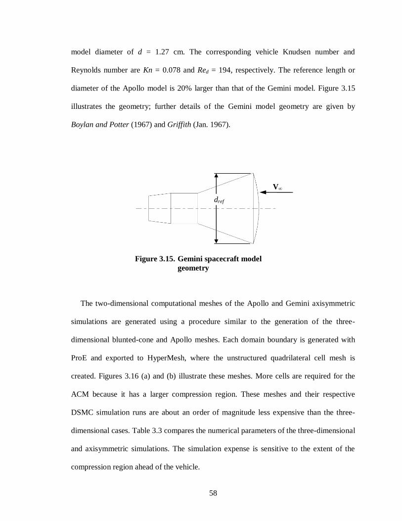
58
model diameter of d = 1.27 cm. The corresponding vehicle Knudsen number and
Reynolds number are Kn = 0.078 and Red = 194, respectively. The reference length or
diameter of the Apollo model is 20% larger than that of the Gemini model. Figure 3.15
illustrates the geometry; further details of the Gemini model geometry are given by
Boylan and Potter (1967) and Griffith (Jan. 1967).
The two-dimensional computational meshes of the Apollo and Gemini axisymmetric
simulations are generated using a procedure similar to the generation of the three-
dimensional blunted-cone and Apollo meshes. Each domain boundary is generated with
ProE and exported to HyperMesh, where the unstructured quadrilateral cell mesh is
created. Figures 3.16 (a) and (b) illustrate these meshes. More cells are required for the
ACM because it has a larger compression region. These meshes and their respective
DSMC simulation runs are about an order of magnitude less expensive than the three-
dimensional cases. Table 3.3 compares the numerical parameters of the three-dimensional
and axisymmetric simulations. The simulation expense is sensitive to the extent of the
compression region ahead of the vehicle.
C L
Figure 3.15. Gemini spacecraft model
geometry
V
dref
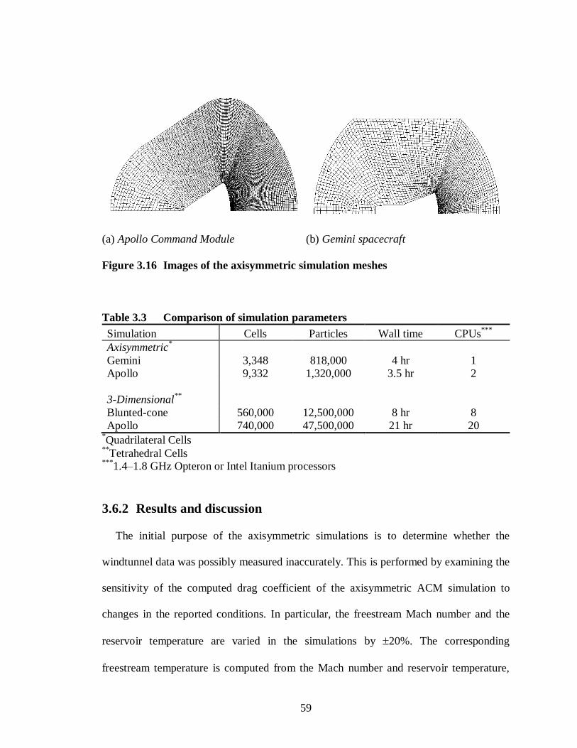
59
(a) Apollo Command Module (b) Gemini spacecraft
Figure 3.16 Images of the axisymmetric simulation meshes
Table 3.3 Comparison of simulation parameters
Simulation Cells Particles Wall time CPUs***
Axisymmetric*
Gemini 3,348 818,000 4 hr 1
Apollo 9,332 1,320,000 3.5 hr 2
3-Dimensional**
Blunted-cone 560,000 12,500,000 8 hr 8
Apollo 740,000 47,500,000 21 hr 20 *Quadrilateral Cells
**Tetrahedral Cells
***1.4–1.8 GHz Opteron or Intel Itanium processors
3.6.2 Results and discussion
The initial purpose of the axisymmetric simulations is to determine whether the
windtunnel data was possibly measured inaccurately. This is performed by examining the
sensitivity of the computed drag coefficient of the axisymmetric ACM simulation to
changes in the reported conditions. In particular, the freestream Mach number and the
reservoir temperature are varied in the simulations by 20%. The corresponding
freestream temperature is computed from the Mach number and reservoir temperature,
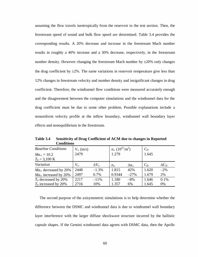
60
assuming the flow travels isentropically from the reservoir to the test section. Then, the
freestream speed of sound and bulk flow speed are determined. Table 3.4 provides the
corresponding results. A 20% decrease and increase in the freestream Mach number
results in roughly a 40% increase and a 30% decrease, respectively, in the freestream
number density. However changing the freestream Mach number by 20% only changes
the drag coefficient by 2%. The same variations in reservoir temperature give less than
12% changes in freestream velocity and number density and insignificant changes in drag
coefficient. Therefore, the windtunnel flow conditions were measured accurately enough
and the disagreement between the computer simulations and the windtunnel data for the
drag coefficient must be due to some other problem. Possible explanations include a
nonuniform velocity profile at the inflow boundary, windtunnel wall boundary layer
effects and nonequilibrium in the freestream.
Table 3.4 Sensitivity of Drag Coefficient of ACM due to changes in Reported
Conditions
Baseline Conditions V (m/s) n (1021
/m3) CD
Ma = 10.2 2479 1.279 1.645
T0 = 3,100 K
Variation V ∆V n ∆n CD ∆CD
Ma decreased by 20% 2448 –1.3% 1.815 42% 1.620 –2%
Ma increased by 20% 2497 0.7% 0.9344 –27% 1.679 2%
T0 decreased by 20% 2217 –11% 1.180 –8% 1.646 0.1%
T0 increased by 20% 2716 10% 1.357 6% 1.645 0%
The second purpose of the axisymmetric simulations is to help determine whether the
difference between the DSMC and windtunnel data is due to windtunnel wall boundary
layer interference with the larger diffuse shockwave structure incurred by the ballistic
capsule shapes. If the Gemini windtunnel data agrees with DSMC data, then the Apollo

61
simulation problem is not likely due to the shock–boundary layer interaction. Figure 3.17
displays selected contour plots from the Apollo and Gemini axisymmetric simulations.
These plots show that the upstream region contains sufficient freestream to capture the
diffuse shock structure near the vehicle and that the peak translational temperature is not
large enough to incur nitrogen dissociation.
(a) Apollo Command Module
Figure 3.17 Translational temperature contour plots of axisymmetric simulations
for the examination of the possibility of shock–wall boundary layer
interaction

62
(b) Gemini Spacecraft
Figure 3.17 Concluded.
Table 3.5 provides comparisons of the windtunnel and axisymmetric simulation drag
coefficients. A result for the ACM from another DSMC code called DS2V, computed by
Dr. Moss, is also listed, and again provides additional credibility to the MONACO
procedures. For the ACM, the axisymmetric simulation drag coefficient is 1.2% larger
than the three-dimensional simulation result. This difference is probably due to
differences in grid cell types and cell distributions between the two and three dimensional
meshes. The difference between the DSMC results and the windtunnel data is an order of
magnitude greater than the difference between the axisymmetric and three-dimensional
results, which is about 11%. The three-dimensional simulation drag coefficient at 180
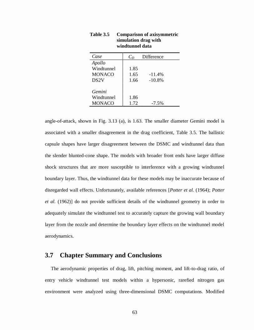
63
Case CD Difference
Apollo
Windtunnel 1.85
MONACO 1.65 -11.4%
DS2V 1.66 -10.8%
Gemini
Windtunnel 1.86
MONACO 1.72 -7.5%
angle-of-attack, shown in Fig. 3.13 (a), is 1.63. The smaller diameter Gemini model is
associated with a smaller disagreement in the drag coefficient, Table 3.5. The ballistic
capsule shapes have larger disagreement between the DSMC and windtunnel data than
the slender blunted-cone shape. The models with broader front ends have larger diffuse
shock structures that are more susceptible to interference with a growing windtunnel
boundary layer. Thus, the windtunnel data for these models may be inaccurate because of
disregarded wall effects. Unfortunately, available references [Potter et al. (1964); Potter
et al. (1962)] do not provide sufficient details of the windtunnel geometry in order to
adequately simulate the windtunnel test to accurately capture the growing wall boundary
layer from the nozzle and determine the boundary layer effects on the windtunnel model
aerodynamics.
3.7 Chapter Summary and Conclusions
The aerodynamic properties of drag, lift, pitching moment, and lift-to-drag ratio, of
entry vehicle windtunnel test models within a hypersonic, rarefied nitrogen gas
environment were analyzed using three-dimensional DSMC computations. Modified
Table 3.5 Comparison of axisymmetric
simulation drag with
windtunnel data

64
Newtonian and free molecular flow models were used to develop procedures to compute
the aerodynamic properties computed by the MONACO DSMC code. For the blunted-
cone windtunnel model, DSMC and windtunnel aerodynamic data agreed well, and a
15% reduction in gas-surface thermal energy accommodation did not significantly affect
the DSMC results. For the Apollo windtunnel test, DSMC and windtunnel data did not
agree well. The drag from DSMC was roughly 13% less than that from the windtunnel
test. For the Apollo simulations, a second set of DSMC results, generated by a different
code, DS2V/3V, provided confidence in the MONACO procedures. Consequently, the
possibility of discrepant Apollo windtunnel test results was examined by a couple of
axisymmetric simulation studies. First, a sensitivity study demonstrated that the drag
coefficient experienced insignificant changes when the reported Mach number or
reservoir temperature was perturbed by 20%. Therefore, the Mach number and reservoir
temperature were considered to be measured accurately enough. Second, a Gemini
windtunnel test simulation was performed to determine whether the problem was related
to windtunnel wall boundary layer interference. This simulation revealed 7.5%
disagreement between the DSMC and windtunnel drag coefficient of the Gemini model.
The disagreement in drag between the DSMC and windtunnel data of the Apollo was
about 50% greater. The Apollo has a 20% larger diameter than the Gemini. Therefore, it
is possible that the windtunnel wall boundary layer interferes with the diffuse shock in
front of the models. However, simulations including the windtunnel wall boundary are
not possible because the available references [Potter et al. (1964), Potter et al. (1962)] do
not provide sufficient details of the windtunnel geometry. In conclusion, aerodynamic
integration procedures were validated and a sensitivity study suggested that the 1960’s

65
windtunnel results of the ACM are potentially affected by wall boundary layer
interference. In the next chapter, an aerodynamic sensitivity study is presented with
simulations of Apollo 6 flight conditions.

66
CHAPTER IV
SENSITIVITY OF AEROTHERMODYNAMICS
PREDICTIONS FOR APOLLO 6 RETURN
AT 110 km ALTITUDE
4.1 Background
In the mid to late 1960’s the Apollo program first tested the Apollo Command Module
(ACM) with unmanned flights that achieved various engineering objectives. The first of
these occurred in February, 1966, with mission AS-201 [Grinter (2005)]. By April, 1968,
the last of the unmanned flights, mission Apollo 6 was conducted. Flight data from the
Apollo 4 and 6 missions were documented by Lee and Goodrich (1972). These missions
involved unmanned test flights of the ACM with entry velocities of roughly 10.0 km/s
into the Earth’s atmosphere. Surface pressure and heating rate history data were gathered
by using pressure transducers, radiometers and calorimeters; however, above 80 km the
data are too scattered for DSMC code validation. Furthermore, below roughly 90 km,
DSMC simulations are exceedingly expensive and the Navier-Stokes equations are
applicable with the appropriate slip boundary condition [Scalabrin (2007)]. Nevertheless,
entry trajectory data provide sufficient information to simulate the Apollo reentry flow
above 90 km with the DSMC method and enable a sensitivity study on the
67
aerothermodynamics by varying physical phenomena in order to gain an understanding of
their significance.
Unlike the wind-tunnel test conditions discussed in the previous chapter, the flight
conditions involve a gas mixture and shock induced energy levels sufficient to incur
chemical reactions. When significant, the chemical activity affects the shock layer flow
and, hence, the momentum and energy transferred to the vehicle. The intensity of
chemical activity is dependent on the density of the freestream flow; thus, it is relevant to
examine whether chemical activity plays a significant role at the rarefied altitudes of the
entry trajectory. At these altitudes, it is also relevant to examine the sensitivity of the
aerothermodynamics to surface radiation and gas-surface accommodation. On the one
hand, a surface radiation boundary condition, instead of an isothermal boundary
condition, will result in a more realistic surface temperature distribution, which may or
may not significantly affect the vehicle aerodynamics. On the other hand, gas-surface
accommodation has a direct effect on the vehicle aerodynamics and varies with flow
regime as the vehicle descends hypersonically into the atmosphere from the free
molecular to the continuum regime. This variation and its effects are not fully
understood. It is necessary to understand these phenomena at rarefied altitudes in order to
correctly predict lift-to-drag ratio and trim angle-of-attack, which are prerequisite for
trajectory planning and thermal protection design [Crowder (1969)]. In this chapter,
simulations of the 110 km entry trajectory point of the Apollo 6 mission are examined.
This altitude is selected because it involves a reasonable simulation expense for multiple
cases. The simulations enable an assessment of the sensitivity of the respective
aerothermodynamics to changes in surface radiation, gas-surface accommodation and

68
chemistry in the flow field due to the diffuse shock layer. To evaluate the effects of the
changes in these physical mechanisms, Mach number contours, temperature contours,
peak field temperatures, surface heating and aerodynamic coefficients are monitored.
This study is presented in the following order: first, a general description of the
simulations is given; second, the effects of varying gas-surface accommodation and wall
temperature boundary conditions are analyzed; third, the effects of gas chemistry are
discussed; and finally, a summary and conclusions are given.
4.2 General Description of the Simulations
Table 4.1 lists the relevant vehicle geometric parameters and freestream flow
conditions, which remain constant throughout the sensitivity study. The dimensions of
the ACM are based on Bertin (1994). However, after a further review of Boylan and
Griffith (1968), Hillje (1967), Lee and Goodrich (1972), Moss et al. (2006) and Park
(1990), it is recommended that this geometry be based on Boylan and Griffith (1968) in
future flight simulations of the Apollo 6. Nonetheless, since this is a sensitivity study of
the effects of physical mechanisms on the aerothermodynamics about the entire capsule,
Table 4.1 Flight conditions
Property Value Property Value
dref 3.91 m Kn 0.26
h 110 km Gas ****
4-species air
155 2 ,Nn
** 1.0510
18 m
–3
V * 9.6 km/s
2 ,On 1.541017
m–3
T **
265 K ,Nn 5.941011
m–3
Ma *** 28.5 ,On 1.2810
17 m
–3
1.003 m
*V is taken from the Apollo 6 trajectory;
** T and ni, are taken from NRLMSIS-00
***Ma, and Kn = / dref are computed with the above freestream data
****This becomes 5-species air when chemical reactions are activated, introducing NO

69
the uncertainty in the aft nose radius, opposite to the heatshield, in the wake region does
not play a significant role. The vehicle shape, angle-of-attack and pitching moment about
the heatshield apex are illustrated in Fig. 4.1. At the 110 km altitude entry trajectory
point, the ACM velocity is 9.6 km/s [Lee and Goodrich (1972)] and its angle-of-attack
is 155 [Hillje and Savage (1968)]. Unknown freestream thermodynamic properties are
determined with the help of the NRLMSIS-00 Earth atmosphere model [Picone (2002)].
The MONACO DSMC code, described in Chapter 2, is employed with the variable soft
sphere collision model [Koura and Matsumoto (1992)] and the variable vibrational
Property Value
Cells 489,055
Particles 33,500,000
Reference time step 1.010–6
s
Number of time steps 40,000
Processors*
16
Wall Time 15 hr *1.4–1.8 GHz Opteron or Intel Itanium processors
Table 4.2 Typical Simulation Expense
Figure 4.1 ACM reference geometry
V
dref
C L
O . CMO

70
energy exchange probability model [Vijayakumar et al. (1999)]. Several simulations of
the ACM at the selected entry trajectory point are made, with varying physical
mechanisms. The expense of a typical simulation is shown in Table 4.2. The simulations
of the 110 km altitude trajectory point are less expensive than the three dimensional
Apollo windtunnel test model simulations presented in Chapter 3, c.f. Table 3.3.
4.3 Sensitivity to Surface Conditions
The sensitivity study begins with a look into the effects of varying gas-surface
accommodation and the temperature boundary condition, while maintaining an inert four
species air model. The first physical mechanism examined is the gas-surface
accommodation. The accommodation is based on the Maxwell gas-surface interaction
model, described in Chapter 5. In this chapter, the model is modified to handle
independent variation of the gas-surface accommodation for translational, rotational and
vibrational energy modes by the accommodation coefficients aM, aE_rot and aE_vib,
respectively. aM represents the probability of a diffuse reflection. If the molecule
reflection is not diffuse, then it is specular. aE_rot and aE_vib represent the probability that
the respective energy modes will be in thermal equilibrium with the solid surface, that is
fully accommodated. The reflected molecule will have either full accommodation or no
accommodation, that is no change, in the rotational and vibrational energy modes.
Initially, full accommodation of the translational, rotational and vibrational energy modes
is assumed. Then, partial accommodation of each energy mode is considered. This is
performed by setting accommodation coefficients of translational, rotational and
vibrational energy to 0.85, 0.10 and 0.01, respectively. The reduced accommodation
values are selected according to the approximate relaxation time for each energy mode.

71
The relaxation times are related to the difference in energy between adjacent quantum
energy states. The energy spacing of translational states is many orders of magnitude
smaller than for rotational states, which are an order of magnitude smaller than for
vibrational states. As a result, the relaxation time to reach translational equilibrium is
beyond an order of magnitude smaller than the relaxation time to reach rotational
nonequilibrium, which is at least an order of magnitude smaller than the relaxation time
to reach vibrational equilibrium. Hence, the time it takes a gas molecule’s vibrational
energy to fully accommodate with the surface must be approximately an order of
magnitude greater than the time its rotational energy takes to fully accommodate and so
forth. This leads to the estimated ratio of accommodation levels between the energy
modes.
In both the full and partial accommodation cases, an isothermal wall temperature is
prescribed by assuming that the incident freestream kinetic energy is completely radiated
at the surface according to the Stefan-Boltzmann law. That is,
3 41
2SB wV T (4.1)
where and SB are the surface emissivity and the Stefan-Boltzmann constant,
respectively. It is further assumed that the surface radiates as a black body, = 1. Thus,
from Eqn. (4.1), a wall surface temperature of 830wT K is specified for the isothermal
wall. The second mechanism examined is the wall surface radiation. This is performed by
repeating the previous cases with a simple radiative equilibrium wall boundary condition
and comparing the results. In the radiative equilibrium wall boundary condition, the wall
temperature is initially set to the isothermal wall temperature of the isothermal wall
cases; then, the convective heat flux given by the DSMC method at a surface element,

72
labeled i, is assumed to be fully radiated by that element according to the Stefan-
Boltzmann law. This assumption provides the wall temperature for the next time step,
n+1, through
4
1
, ,
n n
conv i SB w iq T (4.2)
However, when the convective heat flux results in a wall temperature less than the
vehicle cabin temperature, assumed to be 300 K, the wall temperature is set to the
assumed cabin temperature. In summary, the variations of gas-surface accommodation
and wall surface temperature condition comprise four simulation cases. Table 4.3 assigns
numbers to the simulation cases. To evaluate the effects of changing these surface
conditions on the aerothermodynamics, Mach number contours, temperature contours,
peak field temperatures, wall temperatures, aerodynamic coefficients and maximum
Stanton number are monitored.
Table 4.3 Simulation cases of various surface conditions
Case Gas-Surface Accommodation Wall Temperature
aM aE_rot aE_vib
Isothermal Wall
1 1.00 1.00 1.00 Tw,i = 830 K
2 0.85 0.10 0.01 Tw,i = 830 K
Radiative Equilibrium Wall
3 1.00 1.00 1.00 14, ,
n n
w i conv i SBT q
4 0.85 0.10 0.01 14, ,
n n
w i conv i SBT q
4.3.1 Effects on maximum field and wall temperatures
The sensitivity evaluations begin by looking at the effects on the maximum field and
wall temperatures. Regarding the maximum flow field temperatures of the translational,
rotational and vibrational energy modes, Table 4.4 below shows that decreasing the gas-
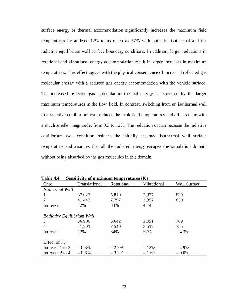
73
surface energy or thermal accommodation significantly increases the maximum field
temperatures by at least 12% to as much as 57% with both the isothermal and the
radiative equilibrium wall surface boundary conditions. In addition, larger reductions in
rotational and vibrational energy accommodation result in larger increases in maximum
temperatures. This effect agrees with the physical consequence of increased reflected gas
molecular energy with a reduced gas energy accommodation with the vehicle surface.
The increased reflected gas molecular or thermal energy is expressed by the larger
maximum temperatures in the flow field. In contrast, switching from an isothermal wall
to a radiative equilibrium wall reduces the peak field temperatures and affects them with
a much smaller magnitude, from 0.3 to 12%. The reduction occurs because the radiative
equilibrium wall condition reduces the initially assumed isothermal wall surface
temperature and assumes that all the radiated energy escapes the simulation domain
without being absorbed by the gas molecules in this domain.
Table 4.4 Sensitivity of maximum temperatures (K)
Case Translational Rotational Vibrational Wall Surface
Isothermal Wall
1 37,023 5,810 2,377 830
2 41,443 7,797 3,352 830
Increase 12% 34% 41%
Radiative Equilibrium Wall
3 36,900 5,642 2,091 789
4 41,201 7,540 3,517 755
Increase 12% 34% 57% – 4.3%
Effect of Tw
Increase 1 to 3 – 0.3% – 2.9% – 12% – 4.9%
Increase 2 to 4 – 0.6% – 3.3% – 1.6% – 9.0%
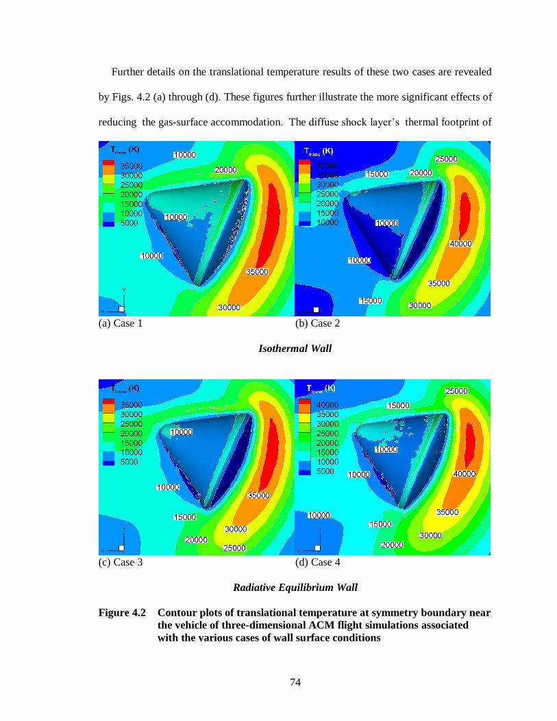
74
Further details on the translational temperature results of these two cases are revealed
by Figs. 4.2 (a) through (d). These figures further illustrate the more significant effects of
reducing the gas-surface accommodation. The diffuse shock layer’s thermal footprint of
(a) Case 1 (b) Case 2
Isothermal Wall
(c) Case 3 (d) Case 4
Radiative Equilibrium Wall
Figure 4.2 Contour plots of translational temperature at symmetry boundary near
the vehicle of three-dimensional ACM flight simulations associated
with the various cases of wall surface conditions
75
translational temperatures above 35,000 K is significantly larger for the cases with
reduced gas-surface accommodation. With the radiative equilibrium surface boundary
condition, the flow temperature distribution over the leeward facing surface involves
lower translational temperatures than the isothermal case. In addition, the flow
temperature distribution next to the radiative surface is sensitive to changes in gas-surface
accommodation, whereas, with the isothermal surface, this distribution is obviously
insensitive to changes in gas-surface accommodation.
Regarding the wall surface temperatures, Table 4.4, above, indicates that the peak
surface temperatures are more affected by switching the wall temperature boundary
condition more than by reducing gas-surface accommodation, although the effects are
within the same order of magnitude. The effects of reducing the gas-surface
accommodation, while maintaining a radiative equilibrium wall, on the wall surface
temperature distribution are illustrated in Figs. 4.3 (a) and (b). This figure shows the
average wall temperature contours based on the average convective heat flux over the
specified steady-state period of the simulation. For both accommodation cases, the
leeward side of the vehicle is essentially isothermal at the assumed cabin temperature of
300 K. The radiative wall partial thermal accommodation case results in slightly cooler
surface temperatures over the heatshield. This effect agrees with the physical
consequence of shorter residence times of the hot gas on the surface required for partial
thermal accommodation.
It is also relevant to note the effects of changing the surface conditions on property
contour plots over the entire computational domain surface of symmetry and on property
profiles along a horizontal line upstream of the vehicle. These perspectives provide

76
(a) Case 3 (b) Case 4
Figure 4.3 Contour plots of wall surface temperature of three-dimensional
ACM flight simulations associated with cases having the
radiative equilibrium wall
further information on the gas behavior. They also provide information on the vehicle’s
influence on the upstream flow field, referred to here as the “upstream domain of
influence”. (This is not to be confused with the domain of influence of the method of
characteristics of supersonic continuum flow analysis. Although there are similarities the
definition here is not intended to be universal.) This region extends from the vehicle out
to the freestream. In continuum hypersonic flow this region is sharply defined by the start
of the bow shock, however, in rarefied hypersonic flow the change in Mach number from
the freestream value occurs gradually due to a diffuse bow shock. For DSMC simulations
above a certain altitude or Knudsen number range, the upstream domain of influence can
vary considerably and indicates the size of the required computational mesh upstream of
the vehicle. The size of the domain downstream of the vehicle need only be large enough
to contain outflow numerical vacuum effects behind the desired geometric region of
analysis.

77
Figures 4.4 (a) through (d) display the entire computational domain surface of
symmetry for each case. The upstream domain of influence of the vehicle on the
surrounding gas translational temperature is increased when the thermal accommodation
is reduced. This effect also agrees with the physical consequence of increased reflected
gas molecular energy with a reduced thermal accommodation for the vehicle surface in
this flow. The increased reflected gas molecular energy allows larger upstream distances
across which information about the vehicle’s presence may travel. However, changing
the wall boundary condition from isothermal to radiative equilibrium has no significant
effect on the upstream domain of influence of the vehicle on the surrounding gas
translational temperature. Similar effects are observed on the vehicle upstream domain of
influence on the surrounding gas Mach number.
(a) Case 1 (b) Case 2
Isothermal Wall
Figure 4.4. Contour plots of translational temperature at entire symmetry
boundary of the three-dimensional ACM flight simulations associated
with the various cases of wall surface conditions

78
(c) Case 3 (d) Case 4
Radiative Wall
Figure 4.4 Concluded
A more detailed perspective is provided by the temperature and Mach number profiles
along a horizontal line, defined by y(x, z) = 1.3 m, upstream of the vehicle (x < 0) and on
the plane of symmetry (z = 0). (The origin of the coordinate system is labeled O in Fig.
4.1.) The horizontal line is located near the horizontal segment of the stagnation stream
line, which changes slightly with each case. The stagnation streamline curves up near the
surface to intersect the stagnation point at y 1.7 m. The respective profiles are shown in
Figs. 4.5 (a) through (d) where x is nondimensionalized by freestream mean-free-path
and shifted such that it is zero at the vehicle surface because the horizontal line does not
intersect the surface at the origin. The profiles provide a clear perspective on how
decreasing the gas-surface thermal accommodation increases the gas energy ahead of the
vehicle, including rotational and vibrational modes. The increases in gas energy extend to

79
the freestream boundaries of the full accommodation cases and, hence, cause the
increases in the vehicle upstream domain of influence.
(a) Translational temperature (b) Rotational Temperature
(c) Vibrational temperature (d) Mach number
Figure 4.5 Temperature and Mach number profiles along a horizontal line ahead
of the ACM, y(x<0, z=0) = 1.3 m, of the three-dimensional flight
simulations associated with the various cases of wall surface conditions

80
4.3.2 Effects on ACM aerodynamics and surface heating
The sensitivity evaluations continue by looking at the effects of the wall conditions on
the ACM aerodynamic coefficients and surface heating. The aerodynamic coefficients of
lift, drag and pitching moment, and the maximum Stanton number are computed for each
of the surface conditions and listed in Table 4.5. The reductions in gas-surface
accommodation cause the aerodynamic forces and moment to increase because of the
increase in gas energy about the vehicle, which causes the resultant aerodynamic force to
increase in magnitude. Also, the increase in specular reflections, according to the
Maxwell gas-surface interaction model, provides an increase in pressure force due to
Table 4.5 Sensitivity of aerodynamics and surface heating
Case CD CL L/D CMO Stmax
Isothermal Wall
1 1.66 0.231 0.139 0.111 0.829 pressure* 1.35 0.511 0.085 shear 0.313 –0.280 0.025
2 1.69 0.275 0.163 0.113 0.700 pressure 1.41 0.532 0.093
shear 0.28 –0.257 0.021
Increase (%) 1.58 18.8 17.0 2.42 – 15.5 pressure 3.77 8.84 6.46
shear –2.17 9.98 –3.96
Radiative Equilibrium Wall
3 1.67 0.232 0.139 0.111 0.858 pressure 1.35 0.513 0.085 shear 0.314 –0.280 0.026
4 1.69 0.274 0.162 0.114 0.712 pressure 1.41 0.531 0.093
shear 0.278 –0.257 0.021
Increase (%) 1.33 17.8 16.2 2.27 – 17.0 pressure 3.50 8.01 6.42
shear –2.17 9.76 –4.15
Increase by changing Tw wall condition
Increase 1 to 3 0.272 % 0.558 % 0.285 % 0.470 % 3.53 %
Increase 2 to 4 0.018 % – 0.355 % – 0.373 % 0.326 % 1.70 % *pressure and shear components of CD, CL and CMO are listed below the total values, percentage increases *in these components are relative to total values of cases 1 or 3 depending on the wall condition

81
rectilinear impact. The aerodynamic forces are due to the pressure and shear stresses on
the vehicle surface. The pressure and shear stresses are affected more by the increased
gas energy ahead of the inclined heat-shield than over the leeward side because of the
larger density ahead of the vehicle. The drag due to pressure is increased, while the drag
due to shear is decreased. The net effect is an increase in the overall drag coefficient.
The increase in lift is partly due to an increase in pressure against the inclined
heatshield. In regard to the shear stresses, the increase in lift indicates that the upward
component of shear in the small region of the heatshield above the stagnation point is
high enough to outbalance the downward component of shear in the larger area below the
stagnation point. The larger increase in lift than in drag indicates that there are larger
increases in positive vertical shear stress components on the part of the heat shield above
the stagnation point, than increases in respective horizontal components in the direction
of the drag force. In terms of Maxwell’s gas-surface interaction model, the increase in lift
is attributed to decreased backward scatter due to decreased diffuse reflections where
specular reflections incur a lift force. This occurs throughout the inclined heatshield
where the angle between the inward surface normal and the freestream is between zero
and ninety degrees.
A significantly larger part of the pitching moment is due to pressure than to shear. The
pitching moment due to pressure increases with the reduction in gas-surface
accommodation, while the component due to shear decreases. The net effect is an
increase in the pitching moment. The increase in pitching moment indicates that the
pressure producing pitch-up moments referenced to point O outbalances the pressure
producing pitch-down moments. The increased pitching moment means that the vehicle is

82
further from the trim angle-of-attack for the reduced gas-surface accommodation and
greater control-system force is required to maintain the specified angle-of-attack.
The location of maximum Stanton number or heat flux is near the location of the
stagnation point. Figure 4.6 below shows contour plots of vertical shear stress and the
location of the maximum Stanton number for case 1. The location of the stagnation point
is at the vehicle vertical plane of symmetry on the zero vertical shear stress contour,
which is zero according to Tecplot contour generation; the cell-centered values come near
to but do not actually reach zero. In Fig. 4.6, the stagnation point is at y 1.60 m; this
varies slightly among the cases. The location of the maximum Stanton number also varies
slightly among the cases. The respective vertical coordinate y of each case is within 5%
of the average, ystag., avg. = 1.67 m. The maximum Stanton number, which is a measure of
the heat flux from the gas to the surface, decreases with accommodation because less
thermal energy is imparted onto the surface in order to accommodate the thermal energy
Figure 4.6 Contour plots of vertical shear stress
location of Stmax, y = 1.64 m, from
case 1

83
of the gas with that of the surface. The decrease in surface heating accompanied by an
increase in lift-to-drag ratio (L/D) agrees with studies by Neumann (1989), which suggest
that increasing L/D decreases peak heating for certain configurations with L/D < 1. In the
present study, L/D increases by about 17% from case 1 to case 2 and by about 16% from
case 3 to case 4; the associated decreases in Stmax are 16% and 17%, respectively. This
demonstrates the sensitivity of the ACM aerodynamics and surface heating to changes in
gas-surface accommodation at this flight condition.
In regard to the change in wall boundary condition from isothermal to radiative, the
aerothermodynamic properties are affected much less, see the bottom of Table 4.5. As
expected, the Stanton number is affected the greatest, though below 4%. The other
properties are affected by less than 0.6%.
4.4 Sensitivity to Chemically Reacting Flow
The sensitivity study ends by examining the effects of introducing gas chemistry into
the flow field. In this section, the results of case 4 are compared with the same simulation
except with chemistry activated, denoted as case 5. For case 5, a set of 19 chemical
reactions is activated using the TCE model. These include the dissociation and exchange
reactions listed in Table 4.6. These reactions introduce a fifth species, namely, nitric
oxide (NO). The dissociation reactions are written in an abbreviated form such that each
reaction represents five reactions corresponding to each identity of species M. The
recombination reactions, which are the reverse of the dissociation reactions, are excluded
because the extremely small chance (~10–10
) that a ternary collision will occur and lead to
a recombination reaction within these flow conditions. The expense of the simulation is

84
Dissociation Reactions Exchange Reactions
N2 + M N + N + M NO + O O2 + N
O2 + M O + O + M N2 + O NO + N
NO + M N + O + M O2 + N NO + O
NO + N N2 + O
M = N2, O2, NO, N or O
similar to the inert case. Indeed, only a small quantity of chemical reactions occurs.
During each time-step, there are about 33.6 million simulation particles. Among these
particles only about 10,800 collisions occur throughout the simulation domain and only
about 0.3% of these result in a chemical reaction.
The sensitivity evaluations of the influence of chemistry are processed by examining
peak field and wall temperatures, and profiles of field temperatures, Mach number and
species number densities. The peak field temperatures, exhibit 5% reductions due to the
chemistry, as listed in Table 4.7. The peak wall surface temperature is not significantly
affected. The small or insignificant changes are a consequence of the small quantity of
chemical reactions due to the low pressure of the rarefied flow.
Table 4.7 Sensitivity of maximum temperatures (K) to flow chemistry
Case Translational Rotational Vibrational Wall Surface
4 (no chemistry) 41,201 7.540 3,517 755
5 (chemistry) 39,183 7,128 3,437 754
Increase – 4.9 % – 5.5 % – 4.2 % – 0.13 %
Property profiles along the line, y(x<0, z=0) = 1.3 m , described in Section 4.3.1,
provide a more thorough observation. Figures 4.7 (a) through (d) are profiles of
translational, rotational and vibrational field temperatures, and of Mach number. These
Table 4.6 Chemical reaction mechanism

85
show that under these conditions chemical reactions only affect small regions near the
peak field temperatures and do not significantly affect the velocity field.
(a) Translational temperature (b) Rotational Temperature
(c) Vibrational temperature (d) Mach number
Figure 4.7 Temperature and Mach number profiles along a horizontal line ahead
of the ACM, y(x<0, z=0) = 1.3 m, of the three-dimensional flight
simulations associated with cases 4 (no chemistry) and 5 (chemistry)

86
Figures 4.8 (a) through (d), illustrate species number density profiles, excluding
monatomic nitrogen for brevity. Increase in monatomic oxygen density suggests
significant dissociation. The rise of nitric oxide density reveals a significant quantity of
(a) diatomic nitrogen (b) diatomic oxygen
(a) monatomic oxygen (b) nitric oxide
Figure 4.8 Species number density profiles along a horizontal line ahead of the
ACM, y(x<0, z=0) = 1.3 m, of the three-dimensional flight simulations
associated with cases 4 (no chemistry) and 5 (chemistry)
87
exchange reactions. Thus, the species profiles show evidence of diverse flow chemistry,
nevertheless, the low pressures do not foster a sufficient quantity of reactions to
significantly affect the ACM surface heating.
Finally, a comment is made about the sensitivity of flow chemistry on the vehicle
aerodynamics and surface heating. The DSMC simulation with flow chemistry, case 5,
produces the same aerodynamic coefficients and surface heating as case 4, to the
indicated level of precision shown in Table 4.5 above. In conclusion, cases 4 and 5 of the
three-dimensional DSMC simulations reveal that chemical reactions at the 110 km entry
trajectory point of Apollo 6 play no significant role on the ACM aerodynamics and
surface heating.
4.5 Chapter Summary and Conclusions
A sensitivity study was executed on the aerothermodynamics of the Apollo Command
Module (ACM) at the 110 km entry trajectory point of the Apollo 6 mission. The study
examined the significance of three physical mechanisms: gas-surface accommodation,
surface radiation and flow chemistry. To evaluate the effects of the changes in these
physical mechanisms, Mach number contours, temperature contours, peak field
temperatures, surface heating and aerodynamic coefficients were monitored. The first two
mechanisms were examined by four simulation cases entailing two gas-surface
accommodation conditions and two surface temperature conditions. With an isothermal
wall, it was found that decreasing gas-surface energy accommodation for the
translational, rotational and vibrational components simultaneously from full to 85%,
10% and 1%, respectively, increases maximum field temperatures by 12%, 34% and 41%

88
for the translational, rotational and vibrational energy modes, respectively. In addition,
this reduction in gas-surface accommodation significantly increased the vehicle’s
upstream domain of influence and significantly affected the ACM aerodynamics: lift
increased by 18% and peak surface heating decreased by 18%. Similar changes were
observed when reducing the gas-surface accommodation while maintaining a radiative
equilibrium wall condition. In contrast, switching the surface boundary condition from
isothermal to radiative equilibrium, while maintaining a constant gas-surface
accommodation, did not significantly affect the flow field temperatures and upstream
domain of influence. In addition, it only slightly affects the vehicle aerothermodynamics:
the lift and maximum Stanton number were increased by about 1%. Nonetheless, the
radiative equilibrium condition did provide more realistic wall surface temperature
distributions for the simulations with little computational expense.
To examine the sensitivity of the aerothermodynamics to flow chemistry, one of the
inert simulations was rerun with MONACO chemistry procedures activated. It was
shown that chemical reactions only affected the diffuse shock region near the peak field
temperatures, which were reduced by 5%. Because of the high temperatures a diverse set
of chemical reactions did occur, nevertheless, the low pressures did not foster a sufficient
quantity of reactions to significantly affect the ACM surface heating and aerodynamics.
Because of the rapid rise in density and pressure with reduction in altitude from 110 km,
chemistry may still play a significant role in DSMC aerothermodynamic analysis at lower
altitudes, hence, the significance of chemistry is yet a relevant question at lower altitudes,
although the DSMC simulations are significantly more expensive there.
89
In conclusion, the sensitivity study of the 110 km entry trajectory point of the Apollo 6
revealed that: changes in the gas-surface thermal accommodation significantly affect the
aerothermodynamics; the addition of surface radiative equilibrium does not significantly
affect the aerothermodynamics; and the inclusion of chemistry does not significantly
affect the aerothermodynamics. Thus, because of the significance of gas-surface
interactions found under these reentry conditions and because the behavior of gas-surface
interactions under rarefied hypersonic conditions is not well understood, the remaining
research in this thesis was directed toward improving the understanding and simulation of
gas-surface interactions under hypersonic rarefied conditions. The next chapter presents
an effort toward this goal.
90
CHAPTER V
ASSESSMENT OF GAS-SURFACE
INTERACTION MODELS
5.1 Introduction
The previous chapter demonstrated the significance of gas-surface interactions on the
aerothermodynamics of space capsule reentry. Aerothermodynamics is governed by the
momentum and energy transferred from the incoming gas flow onto the surface of the
vehicle. These transfers are governed by the collisions between the gas molecules and the
solid surface. The collision process between a gas molecule and a solid surface is termed
a gas-surface interaction. In kinetic theory, the gas-surface interaction forms a boundary
condition between the gas molecules and the solid surface. For scales relevant to kinetic
theory, the gas-surface interactions are usually modeled with parameters having
macroscopic character, in order to have manageable and efficient calculations. The
smallest gas-surface interaction spatial scale considered in this study is on the order of 10
m, based on the minimum computational mesh cell size adjacent to the surface. Gas-
surface interaction models for macroscales can also be augmented by special use of
molecular dynamics [Tsuboi and Matsumoto (2001)].
91
Although various gas-surface interaction models have been proposed over the past
century and a half, the validity of these models remains tenuous for hypersonic rarefied
flow conditions. The study in this chapter employs numerical simulation, using the Direct
Simulation Monte Carlo (DSMC) method, to scrutinize two of the most common gas-
surface interaction models used with the DSMC method: the Maxwell model, and the
Cercignani, Lampis and Lord (CLL) model. In the literature, comparisons of flow field
properties between DSMC and laboratory data of rarefied hypersonic flow are
uncommon. Hence, this study is also intended to generate new comparisons of this kind.
In particular, the study compares shock or boundary layer properties between DSMC and
existing windtunnel data of rarefied hypersonic flow near the leading edge of a flat plate.
These comparisons involve the assessment of the prediction capabilities of the gas-
surface interaction models through parametric analysis of boundary layer velocity
profiles. In addition, the study examines probability distribution plots of the molecular
velocity components at specified points in the flow field, and of molecular angle of
reflection at specified points on the solid surface. The study is presented in the following
order: first, a review of gas-surface interactions models is presented; second, a
mathematical description of the two common models is laid out; third, comparisons are
made between DSMC and compressible boundary layer theory; fourth, the parametric
analysis is presented using contour plots, molecular velocity distributions and boundary
layer velocity profiles; fifth, an examination of the effects of seeded iodine is reported;
sixth, an analysis of nonequilibrium within the boundary layer is presented; seventh
results are presented of DSMC Apollo 6 flight simulations using the Maxwell and CLL
gas-surface interaction models; and finally, the results and conclusions are summarized.

92
5.2 A Chronicle of Models since Maxwell
Historically, the first gas-surface interaction model for kinetic theory is the model
developed by Maxwell (1879). It considers two kinds of interactions, the specular and
diffuse interactions, which are the result of a molecule encountering a perfectly reflecting
or a perfectly absorbing surface, respectively. A specular interaction or reflection occurs
when an incident molecule collides with the molecular structure of a solid surface in such
a way that it rebounds elastically as if hitting a flat surface. This type of collision occurs
when the gas molecule collides with a peak of the solid surface molecular structure,
assuming the gas and solid molecules are rigid elastic spheres. The collision results in an
inversion of the surface normal component of the molecule’s incident velocity and no
change in its tangential components. Thus, the angle of reflection is the same as the angle
of incidence. A diffuse interaction occurs when an incident molecule interacts with the
molecular structure of the solid surface in such a way that it attains thermal equilibrium
with the surface and then evaporates from the surface according to the Maxwellian
velocity distribution at the local surface temperature. The Maxwell model considers a
fraction aM of the incident molecules to be temporarily absorbed by the surface and then
reflected diffusely from the surface; the remaining incident molecules are assumed to
reflect specularly.
Scattering distributions, that is, probability distribution plots of gas-surface reflection
or scattering angle r, the angle between the surface horizon and the molecular velocity
upon departure from the surface, illustrate the scattering trends of gas molecules reflected
from the solid surface. Polar plots of the scattering distribution predicted by the Maxwell
model, for a beam of molecules targeted onto a solid surface at a specified angle of

93
incidence, has a sharp oval due to the specular reflections, as shown by Figure 5.1 (a),
along with a circular shape due to the diffuse reflections, as shown by Figure 5.1 (b).
(a) specular component (b) diffuse component
Figure 5.1 Schematic polar plots illustrating scattering distribution predicted by
Maxwell’s model for a beam of molecules targeted onto a flat surface at
a specified angle-of-incidence i
The composite distribution will then be a circular shape with a protruding peak. If the
molecules in the beam are all traveling at the same velocity, then the peak is a line at the
specular angle of reflection. However, contrary to the expected distributions given by the
Maxwell model, molecular beam experiments, e.g., Schaaf (1963), Hinchen and Foley
(1966), and Knetchel and Pitts (1969), have shown scattering distributions to be petal-
shaped rather than a composition of a circle and a sharp oval. Partly because of molecular
beam experimental findings, various models have been developed to match the observed
scattering distributions. Some of these models also aim at handling non-uniform gas-
surface accommodation, i.e., accommodation dependent on local surface properties such
as inclination angle. For convenience, interaction parameters unique to the model are
commonly employed, in order to examine the model parametrically against laboratory
results.
O O
r
P(r)
i
i

94
Because Maxwell’s model proved suitable for low speed experiments, such as
Millikan (1923), the development of gas-surface interaction models received little
attention from the inception of Maxwell’s model until satellites began orbiting the Earth
and the problem of free molecular drag brought attention to them. In 1959, Schamberg
proposed a surface interaction model for analyzing free molecular flow drag on satellites
traveling at “hyperthermal” speeds, speeds exceeding the mean thermal speed of the
rarefied gas by six times. This model contains three interaction parameters: the energy
accommodation coefficient, a special exponent to relate incident and reflected directions,
and the “beam width” angle. It is an improvement over Maxwell’s model in that it
explicitly considers local gas-surface interaction conditions; however, it is cumbersome
and it assumes a uniform re-emission speed for all directions.
A couple of years later, at the second international symposium on rarefied gas
dynamics, Nocilla (1961) reported a model intended for free molecular flow conditions
where the velocity distribution of reflected particles is assumed to follow a shifted or
“drifting” Maxwellian. Then in 1963 at the same biennial symposium, Nocilla followed
up with a report showing that his model fit closely to laboratory results of scattering
distributions at certain conditions. His model is fitted by varying the reflected molecular
speed ratio and reflected bulk velocity angle relative to the surface normal; an equation
for the energy accommodation coefficient in terms of these parameters is listed near the
end of that report. Although this model makes improvements in mathematical
construction, Nocilla’s model has a major gap by having no correlation between the
incident and reflected velocity distributions.

95
In 1968, Hurlbut and Sherman reported an update to Nocilla’s model by connecting
the incident and reflected distributions. They assume a drifting Maxwellian for the
incident velocity distribution, and relate the incident distribution to Nocilla’s reflected
distribution by equating the inbound and outbound number fluxes. This model, known as
the Hurlbut-Sherman-Nocilla (HSN) model, utilizes the energy accommodation
coefficient, reflected molecular speed ratio and reflected bulk velocity angle for
parametric analysis. In a 1992 report, Hurlbut lays out relations for the normal and
tangential momentum accommodation coefficients in terms of these parameters.
Nevertheless, the way the model connects the incident and reflected fluxes does not
generally agree with the principle of detailed balance for gas-surface interactions.
Knowledge of the standard interaction parameters allows accurate calculations of
aerodynamic and heat transfer coefficients for bodies in free molecular or collisionless
flow. For rarefied flows involving a significant amount of intermolecular collisions, it is
necessary to have knowledge of the re-emitted molecular property distributions. Each
gas-surface interaction model mentioned hitherto provides distributions; however, only
Maxwell’s model generally satisfies the reciprocity principle, defined in Section 5.3.2.
Under the assumption of local equilibrium, the distributions need to satisfy the principle
of reciprocity, which is the principle of detailed balance for gas-surface interactions. A
couple of reports that provide theoretical descriptions of the principle are given by
Kuščer (1971) and Wenaas (1971). This principle is fundamental to a formal
mathematical approach for relating the reflected distributions to the incident distributions
called scattering kernel theory, formally presented for example in the publications of
Cercignani (1969) and Kuščer (1971). At the cost of some restrictions to the model,

96
conformation to the reciprocity principle allows for the application of the H-theorem to
gas-surface interactions, a symmetrized scattering kernel and a simplified boundary
condition.
In 1971, Cercignani and Lampis initially proposed a model, known as the CL model,
which satisfies the fundamental scattering kernel principles. The CL model involves the
tangential momentum and normal kinetic energy accommodation coefficients, and
performs respectably against laboratory results [Cercignani and Lampis (1971);
Cercignani and Frezzotti (1989)] under certain high speed rarefied flow conditions.
Although it compares well only within a limited range of laboratory conditions, the CL
model is theoretically sound and relatively simple. A couple of newer kernels intended to
extend the applicability of the CL model are given by Cercignani et al. (1995) and
Cercignani and Lampis (1997). However, these two kernels employ interaction
parameters that lack clear physical meaning and provide only marginal improvements in
limited comparisons with laboratory experiments. Evidently, a desired empirical
interaction model is in terms of empirical factors or parameters with clear physical
interpretations; two or three of these parameters allow the kernel to have reasonable
agreement with laboratory results over a sufficient range of conditions. In this sense, the
original CL model has not yet been surpassed as the best empirical interaction model for
engineering analysis and remains suitable for theoretical studies Sharipov (2001).
Twenty years after the CL model was initially published, a transformation of the CL
model for use with the DSMC method was laid down by Lord (1991). This
transformation is referred to as the CLL model. The transformation extends the CL model
to handle rotational energy exchange between the gas and the surface. Later, Lord (1991

97
and 1995) further extended the model to handle vibrational energy exchange and a
broader range of scattering states. One of these states is diffuse scattering with partial
thermal energy accommodation. Indeed, there is no physical reason why an incident
molecule has to reflect specularly with a single encounter with the molecular structure of
the surface. The CLL model has now gained wide acceptance; examples of recent
applications are reported by Ketsdever and Muntz (2001), Santos (2006) and Utah and
Arai (2002).
The DSMC method, which reached common acceptance by the 1980s, relies on gas-
surface interaction models at the surface boundaries of the computational domain. For
sufficiently low Knudsen and Mach numbers, the diffuse scattering model suffices.
Outside these conditions, such as the initial phase of spacecraft reentry, it is necessary to
implement a more sophisticated model for the reasons mentioned above. Probably the
two most common models presently in use with the DSMC method are Maxwell’s model
and the CLL model. It is these two models which are examined in this study. Before
proceeding further into the present study, a couple of newer developments are briefly
described to complete this chronicle.
The gas-surface interaction models mentioned so far are based on macroscopic
description. They depend on only a few interaction parameters with values determined by
fitting the models to experimental results. With the continual improvement of advanced
computing systems, the ability to delve into a more detailed phenomenological
description is beginning to become tractable. Two approaches have been taken based on
separate theoretical grounds. Agbormbai (1988 and 2001) has made efforts toward
maturing an approach based on statistical mechanics. This approach conforms with
98
reciprocity, involves ensemble mathematics, enables the specification of a surface energy
distribution and is suitable for DSMC. It involves an ajustable parameter to handle the
scattering from specular to diffuse. It is considered as a generalized Cercignani approach.
However, the approach has been shown to give unrealistic scattering distributions [Lord
(1991)] and has yet to fully mature and gain popularity. Yamanishi et al. (1999) have
developed a multistage gas-surface interaction model for DSMC. In this approach,
scattering parameters are determined from independent molecular dynamics (MD)
simulations. In the DSMC simulation, some of the MD based scattering parameters are
employed with model equations to determine translational and rotational energy
exchange between gas molecules and the solid surface, which enables the calculation of
reflected velocity in the plane defined by the surface normal and the incident molecule
direction. To determine the respective out-of-plane scattering, the procedure employs a
model potential energy surface derived from other MD based scattering parameters.
Molecules then scatter away from the surface, scatter onto another section of the surface
or are “physisorbed” by the surface. The physisorbed molecules are assumed to
eventually emerge diffusely from the surface. For maintaining equilibrium between a
stationary equilibrium gas and a solid surface, diffuse reflection is imposed because the
approach does not generally satisfy reciprocity. With a good molecular dynamics
database the model has been shown to closely agree with laboratory scattering
experiments. This model also has yet to commonly appear in engineering applications.
5.3 Mathematical Description of Two Modeling Concepts
The various gas-surface interaction models that have been proposed since Maxwell’s
model have resulted in a couple of well established concepts presented here. These

99
concepts are used in describing the two common gas-surface interaction models
examined in this study.
5.3.1 Interaction parameters
Parameters employed in gas-surface interaction models are called interaction
parameters. For larger than the nanometer scale, these parameters are relevant to a
macroscopic description; typically, they are accommodation coefficients. An
accommodation coefficient is a numerical description about the degree to which a flow of
gas accommodates kinetically or thermally with a solid surface, while interacting with the
surface. The accommodation coefficient of molecular property Q is defined in terms of
incident and reflected fluxes as follows [Schaaf and Schambré (1961); Gombosi (1994)]:
Q Q
i rQ Q Q
i w
a
(5.1)
where Q
i and Q
r are the incident and reflected fluxes of Q, respectively, and Q
w is the
reflected flux of Q corresponding to full accommodation. Common examples of Q are the
total energy E, normal momentum mn, and tangential momentum mt. The total energy,
normal momentum and tangential momentum accommodation coefficients are defined,
with the usual notation, by , and n tE n m t ma a a , respectively.
5.3.2 Scattering kernel
In kinetic theory analysis, the gas-surface interaction model is used as a boundary
condition. A formal mathematical construct for a gas-surface interaction model is the
scattering kernel formulation, outlined for example by Cercignani (1972). A scattering
kernel ,i rK
represents the probability density that an incident molecule with

100
velocity i
is reflected with velocity r
at essentially the same time and place. It bridges
the velocity distribution functions, i if
and r rf
, of the incident and reflected
molecules, respectively, through the following integral transform:
,
, ,0
,n i
n r r r n i i i i r if f K d
(5.2)
where each gas-surface interaction is independent of others and the average interaction
time is small relative to the temporal evolution of f. In addition, the scattering kernel
satisfies the following three criteria: positivity, normalization and reciprocity. These
criteria are expressed mathematically as follows:
, 0i rK
(5.3)
, 0
, 1n r
i r rK d
(5.4)
, ,, ,n i M i i r n r M r i rf K f K
(5.5)
where fM is the Maxwellian velocity distribution in equilibrium with the solid surface:
23
22 exp2
M G w
G w
f d R T dR T
(5.6)
The product f d
is the probability of any given molecule to have velocity
within the range
and d
. The reciprocity condition [Wenaas (1971); Kuščer
(1971)], Eqn. 5.5, is the equilibrium condition for gas-surface interactions. It must be
satisfied when the flow is in equilibrium with the solid surface.

101
5.4 Mathematical Description of Two Common Models in
Use with DSMC
5.4.1 Maxwell model
The most common model in use with the DSMC method is the Maxwell model. It has
a scattering kernel which satisfies positivity, normalization and reciprocity, and is written
as follows [Cercignani (1969)]:
,, 1M i r M i r specular M M r rK a a f n
(5.7)
where ,r specular
is the molecular velocity of specular reflection. aM is Maxwell’s fraction
as described in Section 5.2. It is an accommodation coefficient that indicates the
probability of a diffuse reflection and does not represent a ratio of fluxes. In the
implementation for the MONACO DSMC code, a reflected molecule’s internal energy
for a diffuse reflection is computed based on thermal equilibrium with the local surface
temperature. For a specular reflection, the molecule’s internal energy for a specular
reflection is assumed unchanged. In other words, in MONACO aE_int = aM for the
Maxwell model.
5.4.2 Cercignani, Lampis and Lord model
As discussed in section 5.2, the best analytical gas-surface interaction model, which
has been shown to match some laboratory scattering distributions, is the CL model
because it involves well defined interaction parameters, namely, parameters that can be
expressed in the form of Eqn. (5.1), and it involves a well defined mathematical
framework, namely, the scattering kernel construction. The CL model interaction
parameters are the accommodation coefficient for the tangential momentum t aQ,
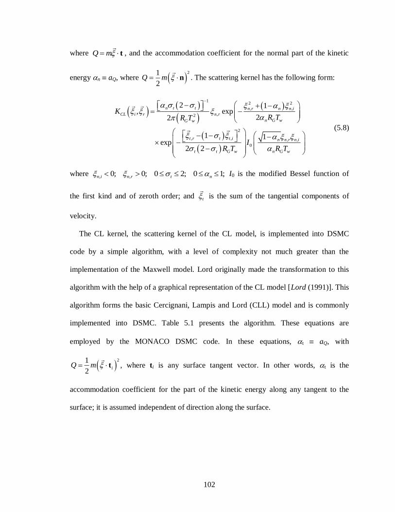
102
where Q m t
, and the accommodation coefficient for the normal part of the kinetic
energy n aQ, where 21
2Q m n
. The scattering kernel has the following form:
12 2
, ,
,2
2
, , , ,
0
2 1, exp
22
1 1exp
2 2
n t t n r n n i
CL i r n r
n G wG w
t r t t i n n r n i
t t G w n G w
KR TR T
IR T R T
(5.8)
where , ,0; 0; 0 2; 0 1;n i n r t n I0 is the modified Bessel function of
the first kind and of zeroth order; and t
is the sum of the tangential components of
velocity.
The CL kernel, the scattering kernel of the CL model, is implemented into DSMC
code by a simple algorithm, with a level of complexity not much greater than the
implementation of the Maxwell model. Lord originally made the transformation to this
algorithm with the help of a graphical representation of the CL model [Lord (1991)]. This
algorithm forms the basic Cercignani, Lampis and Lord (CLL) model and is commonly
implemented into DSMC. Table 5.1 presents the algorithm. These equations are
employed by the MONACO DSMC code. In these equations, t aQ, with
21
2iQ m t
, where ti is any surface tangent vector. In other words, t is the
accommodation coefficient for the part of the kinetic energy along any tangent to the
surface; it is assumed independent of direction along the surface.

103
Table 5.1 Algorithm equations of the CLL model: reflected molecular velocity
components relative to local surface unit vectors
Normal Component Tangent 1
Component
Tangent 2
Component
1 1
2 2
, , ,
2 2
, , 1 , 1 , 2
ln
2
1
2 cos
n
n m n i mp w n
n r mp w n m n m
r x
x
r r
3 3
4 4
, 1, ,
1, , , 3 4
ln
2
1
cos
t
t m t i mp w t
t r mp w t m
r x
x
r
5 5
6 6
2, , 5 6
ln
2
cos
t
t r mp w
r x
x
r
Auxiliary: xi are random numbers uniformly distributed between 0 and 1;
, 2mp w G wR T ; 2t t t
5.5 Flat Plate Windtunnel Test Simulations Using the Two
Models
5.5.1 General description
To examine the gas-surface interaction models, this research involves computer
simulations of existing windtunnel tests examining rarefied hypersonic flow over a flat
surface or plate. The windtunnel tests, reported by Cecil and McDaniel in 2005, use
planar laser induced fluorescence (PLIF) of seeded iodine, within a free jet expansion of
nitrogen, to measure boundary layer flow properties. For details of the windtunnel test
section apparatus, including the geometry of the flat plate windtunnel model refer to the
paper by Cecil and McDaniel (2005).
The computer simulations of the flow-field are performed assuming two-dimensional
flow. In addition, they use rectangular spatial domains that cover a region near the
leading edge of the flat plate, which includes an adequate number of windtunnel test
measurement locations. Each domain is divided into quadrilateral cells or a mixture of
triangular and quadrilateral cells to form two-dimensional computational meshes. The

104
cells have sizes on the order of the local mean-free-path, according to the DSMC
constraint. Throughout each mesh, a uniform particle weight Wp is assigned. The meshes
are generated with HyperMesh (2004) and converted to MONACO readable format with
an in-house grid-conversion code.
To simulate Cecil and McDaniel’s experiment, pure nitrogen is initially assumed. The
corresponding input parameters are listed in Table 5.2. The variables introduced in the
table are: the number of rotational energy degrees of freedom rot, the number of
vibrational energy degrees of freedom vib, the characteristic temperature of vibration vib,
Table 5.2 Physical input parameters for pure nitrogen DSMC simulation
of flat plate windtunnel test
Species Data Collision Cross-Section Data
Species N2 diameter 4.1110–10
m
MW 28.01 11 0.7
rot 2.0
vib 0.0
vib 3390 K
T*
91.5 K Solid Surface Data
Zrot, 18.1 Tw 300 K
the characteristic temperature of the intermolecular potential T*, the maximum rotational
collision number Zrot,, and the viscosity index of the VHS collision model 11 for
collisions between nitrogen molecules.
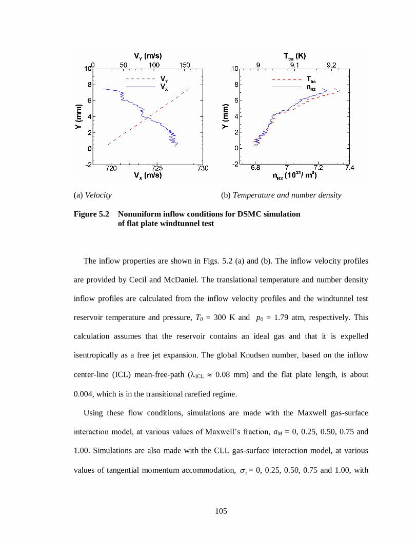
105
(a) Velocity (b) Temperature and number density
Figure 5.2 Nonuniform inflow conditions for DSMC simulation
of flat plate windtunnel test
The inflow properties are shown in Figs. 5.2 (a) and (b). The inflow velocity profiles
are provided by Cecil and McDaniel. The translational temperature and number density
inflow profiles are calculated from the inflow velocity profiles and the windtunnel test
reservoir temperature and pressure, T0 = 300 K and p0 = 1.79 atm, respectively. This
calculation assumes that the reservoir contains an ideal gas and that it is expelled
isentropically as a free jet expansion. The global Knudsen number, based on the inflow
center-line (ICL) mean-free-path (ICL 0.08 mm) and the flat plate length, is about
0.004, which is in the transitional rarefied regime.
Using these flow conditions, simulations are made with the Maxwell gas-surface
interaction model, at various values of Maxwell’s fraction, aM = 0, 0.25, 0.50, 0.75 and
1.00. Simulations are also made with the CLL gas-surface interaction model, at various
values of tangential momentum accommodation, t = 0, 0.25, 0.50, 0.75 and 1.00, with

106
full normal kinetic energy accommodation, n = 1.00. In addition, the sensitivity to
normal kinetic energy accommodation is examined with similar levels of
accommodation, n = 0, 0.25, 0.50, 0.75 and 1.00, while maintaining zero tangential
momentum accommodation, t = 0. Each of the simulations with the CLL model
assumes full internal energy accommodation, E_inta = 1. All of the pure nitrogen
simulations require computational parameters similar to those summarized in Table 5.3.
Table 5.3 Typical computational properties of a pure N2 simulation
of the flat plate windtunnel test
Wp 1.01012 Time-step size 1.010
–8 sec
Particles ~1,915,000 Time-steps 75,000
Cells 19,067 Wall time ~3.5 hr
Processors*
4 *1.4GHz AMD Opteron 240 or 2.8GHz AMD Opteron 254, 1GB RAM per processor
5.5.2 Comparisons with compressible boundary layer theory
Before presenting the comparisons between DSMC and the windtunnel data,
comparisons between DSMC and continuum compressible boundary layer theory, for
two-dimensional flow, are shown in order to illustrate the need for a kinetic
computational method. The validation demonstrates the merit of selecting the DSMC
method based on the global Knudsen number, first mentioned in Section 5.5.1 as 0.004,
which is in the transitional rarefied regime. Comparisons between the computational
methods involve the boundary layer velocity and temperature profiles and the following
surface properties: skin friction and Stanton number. As discussed in Chapter 1, there are
various continuum approaches that can be used to estimate these flow conditions;
however, it is beneficial to begin with a simple approach. Here estimations are made
using continuum boundary layer theory for two-dimensional compressible flow. Because

107
of time constraints, the comparisons are limited to the compressible boundary layer
theory. This boundary layer theory is expected to yield different results. The degree of
these differences is determined in this section.
The two-dimensional compressible boundary layer theory is founded on a set of
boundary layer assumptions for compressible flow. These assumptions reduce the
Navier-Stokes equations to a simplified set of partial differential equations called the
compressible boundary layer equations. These equations are amenable to further
reduction, through a mathematical transformation, to a set of ordinary differential
equations; thus enabling more efficient numerical solution. The transformation reduces
the two-dimensional problem, in terms of spatial coordinates x and y, into a one-
dimensional problem, in terms of a similarity variable ys. The independent variables, x
and y, of the compressible boundary layer equations are transformed into similarity
variables, xs and ys, via the Dorodnitsyn et al. transformation [Anderson (1989)]:
0
x
s e e ex u dx (5.9)
02
ye
s
s
uy dy
x (5.10)
where the subscript e indicates that the quantity is associated with the edge of the
boundary layer. In addition, the dependent variables, x velocity Vx and total enthalpy h,
are converted into the similarity functions, f = f (xs, ys) and g = g (xs, ys), via the following
defining equations:
s e
f u
y u
(5.11)
,s s
e
hg x y
h (5.12)

108
For a flat plate, the form of the momentum and energy boundary layer equations further
reduce such that the similarity functions become functions of only one variable: f (ys) and
g (ys). The compressible boundary layer equations for a flat plate are then a set of
ordinary differential equations as follows:
2 2
2 20
s s s
d d f d fCR f
dy dy dy
(5.13)
2 2
2
11 0
e
e
s s s o s s s
ud CR dg dg d df d ff CR
dy Pr dy dy h dy Pr dy dy
(5.14)
where Pr and CR are the Prandtl number and the Chapman-Rubesin parameter,
respectively. They are defined by the following equations:
pc
Prk
(5.15)
e e
CR
(5.16)
To arrive at Eqns. (5.13) and (5.14), the edge properties ue, Te and pe and the wall
temperature Tw are assumed constant, and the diffusion term in the energy equation is
neglected. For further details of the derivation and method of solution refer to Anderson
(1989) and White (1991). In this section, the similarity solutions are converted back to
physical variables in order to allow comparison with the DSMC solutions.
Comparisons between the boundary layer theory and DSMC for the boundary layer
velocity and temperature profiles are illustrated by Figs. 5.3 (a) and (b), respectively. The
DSMC results with full gas-surface accommodation are chosen because the continuum
theory assumes full accommodation. As expected it is seen that the boundary layer
profiles disagree substantially. The continuum theory results in a substantially larger

109
boundary layer size. In addition, the continuum theory has no slip or temperature jump at
the surface. These conditions delay boundary layer growth, and thus, are a cause of the
smaller boundary layer size given by DSMC. The profile shapes are also distinct. For the
velocity profiles, compressible continuum theory yields a linear shape, whereas DSMC
gives a nonlinear shape. The smaller boundary layer size determined by DSMC also
(a) x velocity
Figure 5.3 Comparison of windtunnel flat plate boundary layer profiles at three
locations downstream from the leading edge. Profiles computed from
continuum compressible boundary layer theory and DSMC.
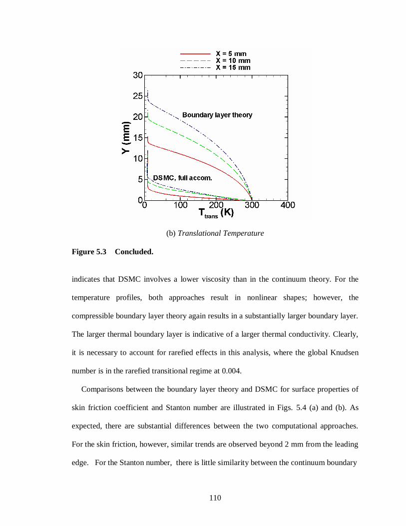
110
(b) Translational Temperature
Figure 5.3 Concluded.
indicates that DSMC involves a lower viscosity than in the continuum theory. For the
temperature profiles, both approaches result in nonlinear shapes; however, the
compressible boundary layer theory again results in a substantially larger boundary layer.
The larger thermal boundary layer is indicative of a larger thermal conductivity. Clearly,
it is necessary to account for rarefied effects in this analysis, where the global Knudsen
number is in the rarefied transitional regime at 0.004.
Comparisons between the boundary layer theory and DSMC for surface properties of
skin friction coefficient and Stanton number are illustrated in Figs. 5.4 (a) and (b). As
expected, there are substantial differences between the two computational approaches.
For the skin friction, however, similar trends are observed beyond 2 mm from the leading
edge. For the Stanton number, there is little similarity between the continuum boundary

111
(a) Skin friction coefficient
(b) Stanton Number
Figure 5.4 Comparison of windtunnel flat plate surface properties between
continuum compressible boundary layer theory and DSMC

112
layer theory and the DSMC method. This again shows the need to account for rarefied
effects in these transitional rarefied conditions.
5.5.3 Contour plots
The variation of Maxwell’s fraction aM from fully specular to fully diffuse results in a
variation in boundary layer size from non-existent to maximum extent. Part of this
variation is illustrated by the half and fully diffuse cases in Figs. 5.5 (a) and (b). These
figures also illustrate the nonuniform inflow boundary through streamlines of bulk flow
velocity. A similar variation in boundary layer size is given by the parametric analysis
with the CLL model involving the variation in tangential momentum accommodation t,
with full normal kinetic energy accommodation n = 1, except that the boundary layer
does not completely disappear at t = 0.
(a) aM = 0.5 (b) aM = 1.0
Figure 5.5 Contour plots and streamlines of flow speed at two values
of Maxwell’s fraction
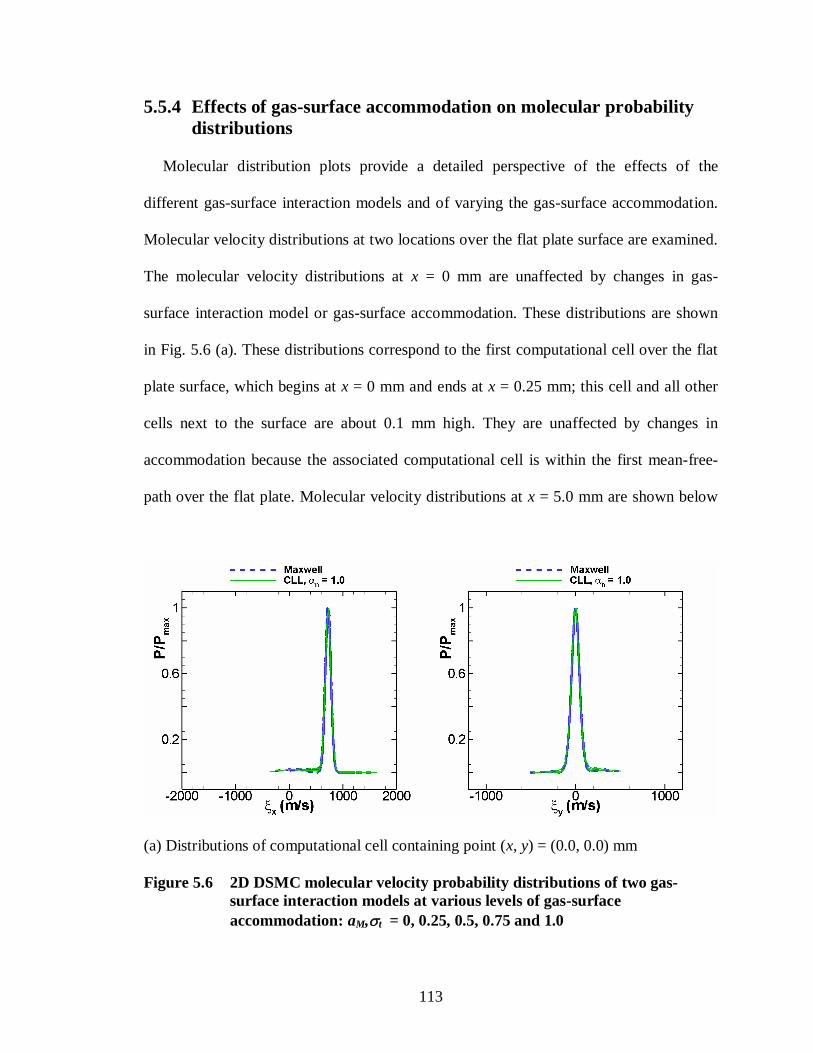
113
5.5.4 Effects of gas-surface accommodation on molecular probability
distributions
Molecular distribution plots provide a detailed perspective of the effects of the
different gas-surface interaction models and of varying the gas-surface accommodation.
Molecular velocity distributions at two locations over the flat plate surface are examined.
The molecular velocity distributions at x = 0 mm are unaffected by changes in gas-
surface interaction model or gas-surface accommodation. These distributions are shown
in Fig. 5.6 (a). These distributions correspond to the first computational cell over the flat
plate surface, which begins at x = 0 mm and ends at x = 0.25 mm; this cell and all other
cells next to the surface are about 0.1 mm high. They are unaffected by changes in
accommodation because the associated computational cell is within the first mean-free-
path over the flat plate. Molecular velocity distributions at x = 5.0 mm are shown below
(a) Distributions of computational cell containing point (x, y) = (0.0, 0.0) mm
Figure 5.6 2D DSMC molecular velocity probability distributions of two gas-
surface interaction models at various levels of gas-surface
accommodation: aM,t = 0, 0.25, 0.5, 0.75 and 1.0

114
(b) Distributions of computational cell containing point (x, y) = (5.0, 0.0) mm
Figure 5.6 Concluded.
in Fig. 5.6 (b). This figure illustrates that the degree of translational nonequilibrium next
to the surface is proportional to the level of gas surface accommodation. It also shows
that the Maxwell and CLL models give identical results only for full gas-surface
accommodation, aM = t = 1.0. At partial levels of gas-surface accommodation, the
models yield similar x distributions. However, the y distributions, at y > 0, are
significantly different.
The molecular surface scattering plots are also examined at the two positions x = 0 and
5.0 mm over the flat plate surface. These are probability distribution plots of reflected
molecule scattering angle r. Figures 5.7 (a) through (d) present the distributions. The
scattering plots show the essential differences between the Maxwell and CLL gas-surface
interaction models. The Maxwell scattering distributions have unrealistic peaks due to the
specular angle at partial levels of accommodation; the associated diffuse component of
the scattering distribution is evident by the circular segments. The CLL scattering

115
(a) x = 0 mm (b) x = 5.0 mm
0 and 25% accommodation
(c) x = 0 mm (d) x = 5.0 mm
50, 75 and 100% accommodation
Figure 5.7 2D DSMC probability distributions of reflected molecular velocity
angle of two flat plate surface faces, y = 0 mm, of two gas-surface
interaction models at various levels of gas-surface accommodation

116
distributions are petal-shaped, similar to observations of reflected rarefied molecular
beams from clean flat surfaces [Schaaf (1963); Hinchen (1966)]. As required, the scatter
plots further confirm that both models are equivalent at full accommodation. There, they
yield the Lambert or cosine distribution of optics theory, which also applies to the
random distribution of gas-surface scattering angles. These plots also show variations in
scattering due to variations in accommodation and position x along the flat plate surface.
The Maxwell distributions have abrupt changes with increasing accommodation and
position; in contrast, the CLL distributions vary smoothly with accommodation and
position. Using the CLL model the changes due to position are remarkably more subtle.
5.5.5 Effects of gas-surface accommodation on boundary layer velocity
profiles
For each of the simulations, data are extracted along vertical slices corresponding to
the locations where PLIF measurements were taken, x = 0, 2.5, 5, 7.5, 10, 12.5, 15, 17.5
and 20 mm from the leading edge. These data include x and y velocity components.
Figures 5.8 (a) through (e) present some of the comparisons between the MONACO
parametric results and the PLIF data. Various observations are made about the results.
Figure 5.8 (a) compares the DSMC and measured velocity profiles at the leading edge
of the flat plate. The fact that the simulations match the experimental data here indicates
that the correct inflow conditions are employed. Furthermore, Figs. 5.8 (a) through (e)
indicate that the data agree in the freestream region above the boundary layer.
The boundary layer is where the flow-field is affected by different gas-surface
interaction models and different levels of gas-surface accommodation. When full gas-
surface accommodation conditions are specified, by setting all accommodation

117
coefficients equal to one, the Maxwell and CLL models provide the same boundary layer
profiles, as expected from the definition of the models. In addition, the Maxwell and CLL
models yield essentially the same results for aM = t = 0.5 and 0.75. However, the
(a) Boundary layer profiles at x = 0 mm
(b) Boundary layer profiles at x = 5 mm
Figure 5.8 Comparison of boundary layer velocity profiles between flat plate
windtunnel tests and DSMC simulations with different gas-surface
interaction models at various levels of accommodation
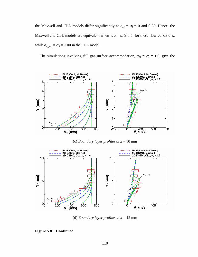
118
the Maxwell and CLL models differ significantly at aM = t = 0 and 0.25. Hence, the
Maxwell and CLL models are equivalent when aM = t 0.5 for these flow conditions,
while E_inta = n = 1.00 in the CLL model.
The simulations involving full gas-surface accommodation, aM = t = 1.0, give the
(c) Boundary layer profiles at x = 10 mm
(d) Boundary layer profiles at x = 15 mm
Figure 5.8 Continued

119
(e) Boundary layer profiles at x = 20 mm
Figure 5.8 Concluded
overall best agreement with the measured data for the Vx profiles, except at the transition
from the boundary layer to the freestream, which is affected by the diffuse shock. The Vx
DSMC results, even for the diffuse case, disagree with the measured data at x 15 mm.
This is due to an adverse pressure gradient believed to be caused by windtunnel test flow
phenomena, beyond the specified computational domain, and thus, not captured by the
simulation. The simulations with aM = t = 0.75 provide the overall best agreement with
the measured data for the Vy profiles, and the Vx profiles in the transition from the
boundar layer to the freestream. Hence, the level of accommodation that provides the
overall best agreement among both the Vx and Vy profiles is a compromise between 0.75
and 1.0. Simulations with the average accommodation, aM = t = 0.875, result in profiles
lying in the middle, in accord with the linear variation of the profiles with
accommodation, when the accommodation level is greater than 0.5. Hence, the overall
120
best agreement, among the considered accommodation levels of the aM or t sensitivity
studies, occurs when aM = t = 0.875.
The large prediction of accommodation is a reasonable prediction from two
perspectives. From physical reasoning, it makes sense that gas-surface accommodation is
incomplete at rarefied hypersonic conditions because of the relatively short average
residence times of the gas-molecules with the flat surface. Conversely, full gas-surface
accommodation occurs for conditions with continuum densities and low velocities. The
degree of accommodation decreases with increase in incident velocity and decrease in gas
density; and also smaller surface roughness. The accommodation of this flow condition is
expected to be relatively high because of the relatively high gas density, similar to
density of air at 60 km altitude according to US 1976 standard atmosphere [Lide (2007)].
The large prediction of accommodation is also reasonable from laboratory or flight
measurements. Measurements from satellites, which are exposed to gases with higher
velocities and much lower densities, show the gas-surface accommodation to be near full
[Minton et al. (2004); Moe (2005) and Moe et al. (1998)]; in particular, Moe (2005)
reports that satellites measure energy accommodation that is near unity at about 155 km
perigee altitude. Furthermore, Cook et al. (1996) measured large levels of momentum
accommodation in experiments involving rarefied molecular beams of nitrogen and
hydrogen with incident velocities of over 1000 m/s, and small incidence angles (< 45)
with finer surfaces or at any incidence angle with rougher surfaces.
The sensitivity study of normal kinetic energy accommodation coefficient n,
confirms that Vx, the tangential component of velocity, is not significantly affected. The
variation of n does affect Vy, the normal component of velocity, but to an order of

121
magnitude smaller extent than the same variation of t. This study indicates that it is
possible to improve the agreement in Vy, between the CLL simulation with t = 1.0 and
the measured data, by significantly reducing n; however, there is no indication in the
experiments found in literature, or even in physical reasoning, that low normal kinetic
energy accommodation would occur along with full tangential momentum
accommodation t. In 1994, Gombosi states that the normal accommodation is relatively
unknown and usually assumed equal to unity. Hence, this case can not be favored over
the t = 0.875 case.
5.5.6 Seeded iodine simulations
The simulations involving pure nitrogen provide good agreement with the PLIF
windtunnel test data using a proper specification of gas-surface accommodation, within
the boundary layer region not affected by the adverse pressure gradient. However,
because the PLIF data reflects the velocity of the seeded iodine, it is possible that the
PLIF data itself is unrepresentative of the nitrogen flow in the windtunnel test. Because
the accuracy of the gas-surface accommodation prediction is sensitive to the accuracy of
the measured data, simulations are run to examine whether the seeded iodine accurately
represents the nitrogen flow velocity. The iodine input parameters for these simulations
are listed in Table 5.4. The values of T*, Zrot,, diameter and 22, for iodine, are taken from
a report by Boyd et al. (1994). The subscripts 1 and 2 on the VHS collision model
viscosity index ij represent N2 and I2, respectively. ij represents the viscosity index for
collisions between species i and j.
122
Table 5.4 Iodine input parameters for seeded iodine DSMC simulation
of flat plate windtunnel test
Species Data Collision Cross-Section Data
Species I2 diameter 8.8010–10
m
MW 253.81 22 0.945
rot 2.0 12 0.8
vib 1.8
vib 306.9 K
T*
557.0 K Solid Surface Data
Zrot, 75 Tw 300 K
The inflow properties for nitrogen are the same as in Figs. 5.2 (a) and (b). The inflow
profiles for iodine are also the same, except for the number density. The inflow number
density for iodine is determined by multiplying the nitrogen number density by the
mixing ratio of iodine to nitrogen. The windtunnel tests held this value at roughly 3.5
10–4
[Cecil and McDaniel (2007)]. Because of the small mixing ratio of iodine to
nitrogen, a species weighting factor is assigned to the iodine, Wp,iodine = 3.5 10–4
, in
order to reduce statistical scatter of the iodine results. It is given a value equal to the
mixing ratio so that the number of simulated iodine molecules is equal to the number of
simulated nitrogen molecules passing through the computational domain. The MONACO
procedure enabling trace species weighting factors is credited to Burt (2006).
With these flow conditions, a simulation is made with full gas-surface
accommodation. For simplicity, the Maxwell gas-surface interaction model is used with
aM = 1.00. This simulation requires the computational parameters summarized in Table
5.5. They are vastly more expensive than the pure nitrogen simulations; the added
expense comes from the necessity of smaller cell sizes due to the smaller mean-free-path
of the iodine. In fact, to keep the simulation manageable the simulation domain is
reduced by roughly 75%, as illustrated by Fig. 2.1 in Chapter 2.

123
Table 5.5 Computational properties of N2 and seeded I2 simulation
of the flat plate windtunnel test
Wp 2.01010 Time-step size 5.010
–9 s
Particles ~62,800,000 Time-steps 150,000
Cells 514,809 Wall Time ~35 hr
Processors*
30
Figures 5.9 (a) and (b) illustrate the computational domain and contour plots of mean-
free-path for each species. The origin of the xy coordinate system is at the leading edge of
the flat plate. The iodine mean-free-path is roughly an order of magnitude smaller
throughout the computational domain. This is a consequence of the dependency on
molecular weight and collision cross-section of the variable hard sphere mean-free-path
in a gas mixture [Bird (1994)]. Even though the mixture mean-free-path is essentially
unchanged with the introduction of seeded iodine, the mean-free-path of the iodine itself,
which is about an order of magnitude smaller than the nitrogen mean-free-path, reduces
the required computational cell sizes in order to correctly simulate the iodine progression
through the flow field.
(a) Nitrogen
Figure 5.9 Contour plots of mean-free-path, with flow speed streamlines, for
nitrogen and iodine at full gas-surface accommodation

124
(b) Iodine
Figure 5.9. Concluded.
Figures 5.10 (a) and (b) illustrate the flow characteristics with contours and
streamlines of flow speed for each species. They indicate that the iodine velocity field is
very similar to the nitrogen velocity field. They also show that these velocity fields are
similar to the pure nitrogen velocity field with full gas-surface accommodation presented
in Fig. 5.5 (b) near the leading edge. This is expected from the small (~10–4
) mixture ratio
(a) Nitrogen
Figure 5.10 Contour plots and streamlines of flow speed for nitrogen and iodine
at full gas-surface accommodation

125
(b) Iodine
Figure 5.10 Concluded.
of iodine to nitrogen and corroborates the windtunnel PLIF measurement procedure. The
figures also expose the effect of the outflow boundary on the flow field. Beyond x 12.5
mm, the contours are affected by presence of the simulation outflow boundary and the
results there do not represent the windtunnel test.
Figures 5.11 (a) through (f) compare boundary layer velocity profiles among pure
nitrogen simulations, nitrogen with seeded iodine simulations, and windtunnel test
measurements. The simulation and windtunnel test data agree within the freestream as
required for a correct simulation. The profiles match at x = 0 mm, except very near the
surface where the simulation profiles exhibit the beginning of the boundary layer and the
iodine component indicates a larger slip velocity due to the larger molecular weight of the
iodine. At x = 0 mm, the pure and component nitrogen profiles are identical. This again is
due to the small mixture ratio of iodine to nitrogen.
At x > 0, several observations about the comparisons are made. The component
nitrogen profiles are almost identical to the pure nitrogen profiles. There are slight
126
differences near the “knee” of the Vy profiles, where the diffuse oblique shockwave lies.
These differences occur for x > 2.5 mm or within 28 and 150 nitrogen and iodine
respective local mean free path distances from the leading edge and are due to the
presence of iodine in the mixture simulations.
(a) Boundary layer profiles at x = 0 mm
(b) Boundary layer profiles at x = 2.5 mm
Figure 5.11 Comparison of boundary layer velocity profiles among pure nitrogen
and nitrogen-seeded iodine MONACO simulations, with full gas-
surface accommodation, and PLIF windtunnel test data

127
The shock is observed near the edge of the boundary layer and is more pronounce in
the Vy profiles than in the Vx profiles. This is expected by the acute angle of the oblique
shock. The Vy plots illustrate that in the boundary layer Vy is accelerated to a value greater
than Vy in the freestream and that the oblique shock bridges these velocities.
(c) Boundary layer profiles at x = 5.0 mm
(d) Boundary layer profiles at x = 7.5 mm
Figure 5.11 Continued
128
For the Vx profiles, largest differences between the nitrogen and the iodine profiles
occur at x= 2.5 mm, however, the profiles converge near the surface and display the same
slip velocity. The differences are mainly due to the larger inertia of iodine causing it to
maintain a slightly larger x velocity component as it blows over the flat plate. Beyond x =
(e) Boundary layer profiles at x = 10 mm
(f) Boundary layer profiles at x = 12.5 mm
Figure 5.11 Concluded

129
2.5 mm, the differences between the nitrogen and iodine Vx profiles are insignificant.
Differences between the nitrogen and iodine Vy profiles occur only at the “knee”
caused by the diffuse oblique shockwave. These differences are greatest at x = 2.5 mm,
more significant than in the Vx profiles, and again decrease beyond x = 2.5 mm. These
differences are again mainly due to the larger inertia of the iodine, in this case, slowing
its ascent caused by the boundary layer expansion underneath the diffuse oblique
shockwave. The differences between the nitrogen and iodine Vy profiles account for some
of the differences between pure nitrogen simulation and the windtunnel data in these
profiles. However, at x 10 mm, the effect of iodine is no longer sufficient to translate
the entire “knee” within the windtunnel data uncertainty envelope.
In summary, the seeded iodine simulations indicate that the iodine merely slightly
affects the Vx profiles within the boundary layer at x 2.5 mm because of the small
(~10–4
) mixture ratio of iodine to nitrogen; this corroborates the PLIF measurements of
the nitrogen flow. For the Vy profiles, the seeded iodine profiles are distinct where the
diffuse shock resides and account for some of the differences between the pure nitrogen
simulation and windtunnel test data. The distinction is mainly due to the larger molecular
weight of the iodine. In the relatively small segments where there are differences, the
iodine profiles generally provide closest agreement with the windtunnel data, as
expected. The inertia effects decrease as x increases beyond 2.5 mm. The result of these
effects is to increase the computed accommodation level which gives the overall best
agreement between the DSMC and measured data, however, rounded to one decimal
place, aM = t 0.9 remains the optimized estimate for the gas-surface accommodation.

130
In conclusion, the seeded iodine simulation revealed the following: the larger
molecular weight and collision cross section of iodine cause an order of magnitude
increase in simulation expense over the pure nitrogen simulations; the larger seeded
iodine inertia partly explains differences in the pure nitrogen simulations and windtunnel
test measurements; and because the overall differences are slight, the seeded iodine
simulation substantiates the pure nitrogen simulations and accredits the PLIF
measurements.
5.5.7 Analysis of thermal nonequilibrium in the boundary layer
In the contour and boundary layer simulation plots, the flow velocity is the local mean
molecular velocity. The PLIF boundary layer plots also involve the local mean molecular
velocity which is an accurate representation of bulk velocity in translational equilibrium.
A system of molecules in translational equilibrium has each of their velocity components
distributed in a Gaussian distribution, that is, a normal distribution. This is a Maxwellian
velocity distribution. For rarefied transitional flows, there may be regions with
translational nonequilibrium. A system of molecules in translational nonequilibrium has
at least one of their velocity components distributed in a non-normal distribution, e.g., a
distribution with multiple peaks or with a skewed shape. Thus, the mean molecular
velocity is not generally an adequate representation of the molecular velocity distribution
in translational nonequilibrium. Thus, in translational nonequilibrium attention is given to
the anisotropic translational temperature tensor components. The degree to which the
velocity distribution is Maxwellian indicates the utility of employing the mean velocity to
represent the bulk velocity of the local system of gas molecules. The extent of
translational nonequilibrium is indicated by differences in component translational
131
temperatures or differences between the mean and most probable local molecular
velocities. Knowledge of where the mean velocity is an inaccurate representation due to
translational nonequilibrium enables a more accurate interpretation of the corresponding
flow conditions. Hence, molecular velocity distribution statistics and distribution shape
and translational temperature profiles are examined at specified points to gauge for
translational nonequilibrium and to explicitly illustrate the relation among these metrics.
In addition, rotational temperature profiles are examined to gauge for rotational
nonequilibrium within the flow field. In the following analysis, full gas-surface
accommodation is assumed because it yields the greatest amount of thermal translational
nonequilibrium in that it statistically incurs the greatest changes in normal and tangential
kinetic energy and in rotational energy. Since the Maxwell and CLL models are
equivalent at full gas-surface accommodation, the results from the Maxwell model are
arbitrarily chosen for the analysis that follows and are referred to as the full gas-surface
accommodation results. The analysis begins with examining the spatial variation of
thermal nonequilibrium in the x direction at selected y; and then, ends with examining the
spatial variation of thermal nonequilibrium in the y direction at selected x.
Table 5.6 presents statistics of molecular velocity probability distributions at selected
computational cells along the x direction and next to the flat plate at y = 0 mm. These
cells have their centers at a height of y = 0.06 mm from the surface. The statistics have
various trends associated with increasing x position. The number of samples lowers with
x because of fewer simulation molecules associated with the lower density in the
expanded flow. The variation of percentage difference between the mean and most

132
Table 5.6 2D DSMC statistics of molecular velocity distributions at y = 0 mm for
various values of x with full gas-surface accommodation x No. of x y
(mm) Samples S. D.* Mean M. P.† %Diff ‡ S. D. Mean M. P. %Diff
0 6,441,210 217.8 636.0 747.0 16.1 109.2 16.5 9.6 52.3
2.5 4,387,893 335.7 403.4 705.2 54.5 204.3 6.6 -35.5 290.9
5.0 3,299,356 333.2 251.2 394.0 44.3 234.6 3.4 -69.3 220.9
7.5 2,752,768 326.8 201.1 308.3 42.1 256.2 1.4 -109.0 205.0
20 1,255,890 299.3 217.1 258.7 17.5 273.3 -6.6 -147.5 182.9 *standard deviation †most probable value ‡percentage difference between Mean and M. P.
probable values suddenly increases at x = 2.5 mm and subsequently lowers with x. This
percentage difference indicates the degree of translational nonequilibrium, which in this
case is due to the initial wave of rebounding molecules from the flat plate surface. At
equilibrium, the percentage difference is zero by definition. The cause of the tendency
towards equilibrium, after the initial disturbance of reflected molecules, is attributed to
more evenly balanced forward and backward scatter from adjacent cell boundaries, at
positions further into the interior of the surface, which is due to continued collisions
caused by scattered molecules. The larger percentage difference and standard deviation of
the y distributions is attributed to the more significant change in the normal component
of momentum due to collision with the surface. The standard deviation, which is
indicative of the distribution spread, does not necessarily vary directly with the
percentage difference: whereas, direct variation is found for thex distributions, inverse
variation is found for the y distributions, between x = 2.5 and 20 mm; that is, as x
increases from 2.5 mm, the standard deviation in the y distribution increases, while the
respective percentage difference between the mean and most probable value decreases.
Figures 5.12 (a) through (d) illustrate the normalized probability distributions,
corresponding to Table 5.6. At the computational cell adjacent to the leading edge, x = 0
mm, both the x and y distributions are near normal. Here, they are not significantly
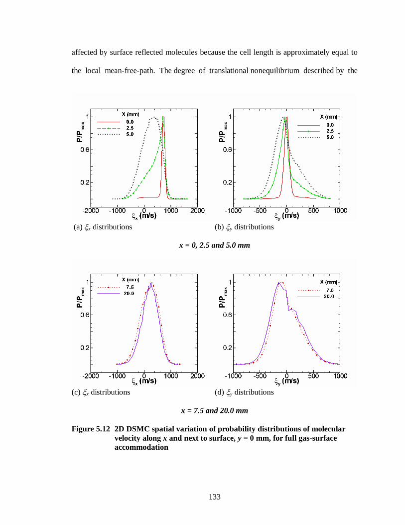
133
affected by surface reflected molecules because the cell length is approximately equal to
the local mean-free-path. The degree of translational nonequilibrium described by the
(a) x distributions (b) y distributions
x = 0, 2.5 and 5.0 mm
(c) x distributions (d) y distributions
x = 7.5 and 20.0 mm
Figure 5.12 2D DSMC spatial variation of probability distributions of molecular
velocity along x and next to surface, y = 0 mm, for full gas-surface
accommodation

134
distribution shape agrees with the trend in percentage difference between the mean and
the most probable values. The trend reflects the evolution of the balance between forward
scatter from the surface to the left of the left boundary of a computational cell and
backward scatter from the surface to the right of the right boundary of the cell. At x = 2.5
mm, the x distributions are significantly skewed. At x = 5.0 mm, the x distribution are
only slightly skewed. By x = 7.5 mm, the x distributions have returned to a near normal
shape. Molecules that traverse this distance will encounter an average of roughly 21
collisions, according to the computed local mean-free-path values. In contrast with the x
distributions, the y distributions remain in translational nonequilibrium along the entire
length of the flat plate beyond the leading edge. Observation of the y distributions in
Figs. 5.12 (b) and (d) reveal that the influence of surface reflection slowly increases from
an enlarged tail at x = 2.5 mm to a second peak at x = 20 mm. The two peaks at x = 20
mm are due to the incident number flux and the surface reflected number flux. The rise of
the second peak is also due to the presence of a backward facing step at x = 20, associated
with the end of the flat plate model and the beginning of the sting, shown in Fig. 5.5. The
backward facing step causes the flow to abruptly expand. This deflects the bulk velocity
streamlines slightly downward within a few mean-free-paths of the backward facing step;
hence, causes incident flux distribution to shift further toward negative y and expose the
peak of the reflected flux distribution. It is also possible that a recirculation vortex in the
backward facing step causes small numbers of simulation molecules to backscatter into
the last computational cell before the backward facing step; and hence, contribute to the
positive y distribution.

135
Another view of translational nonequilibrium is given by profiles of x and y
translational temperature. These are translational temperatures associated with the x and y
random molecular speeds and given by Eqns. 2.2, shown in Chapter 2. Figures 5.13 (a)
and (b) illustrate the variation of translational and rotational temperatures at two distances
above the flat plate surface. The profiles at y = 0 mm represent the computational cells
within one mean-free-path of the flat plate and indicate there is considerable translational
and rotational nonequilbrium. The translational nonequilibrium is demarcated by the
differences among the total translational temperature, and the x and y translational
temperatures. By definition, these temperatures are all equal for translational equilibrium.
Ahead of the flat plate, x < 0, it is seen that the flow is essentially in translational
equilibrium. As the molecules cross over the leading edge, translational and rotational
nonequilibrium suddenly appear among them. In addition, the temperatures abruptly rise.
(a) y = 0 mm (b) y = 2.0 mm
Figure 5.13 2D DSMC translational and rotational temperature profiles along x
at two heights y above the flat plate using full gas-surface
accommodation
136
The rise in temperatures is attributed to the much warmer surface temperature ( 300 K )
than the freestream temperature ( 9 K ). Afterwards, the temperatures of the molecules
near the surface approach the uniform flat plate temperature as they collide with
additional scattered molecules. The rise in the translational nonequilibrium is attributed to
collisions incurred by surface scattered molecules, as described above by the molecular
velocity distributions. This causes the continued flow of molecules to experience a
reduction in the mean molecular speed x ; hence, an increase in the random molecular
speed x x x and hence an increase in Tx. Since most of the flow momentum is
directed along x, the change in the mean vertical molecular speed due to the scattered
molecules is smaller; hence, a smaller increase in Ty occurs. The slower changes in
rotational temperature than in the translational temperature is attributed to the slower
rotational relaxation rate than the translational relaxation rate, predicted by quantum
mechanics. The extent of the themal nonequilibrium is indicated by size of the
differences in the component temperatures. Beyond the leading edge and diffuse shock,
the thermal nonequilibrium steadily diminishes as the flow progresses further over the
flat plate because of continued collisions and thus energy exchanges.
Further above the flat plate, as shown in Fig. 5.13 (b), rotational nonequilibrium does
not appear significantly, however, translational nonequilibrium still appears, though to a
lesser extent and with smoother changes. At y = 2.0 mm, the rise in translational
nonequilibrium is due to the diffuse shockwave, located about 4.0 mm downstream of the
leading edge because it is oblique. The effect of the backward facing step is diffused,
while the extent of translational nonequilibrium appears frozen as gas blows past the flat
plate.

137
The analysis of nonequilibrium now shifts to the examination of the vertical spatial
variation at specified locations x. Consideration is again first given to the molecular
velocity distributions. Figures 5.14 (a) and (b) present the evolution of molecular velocity
distributions with y, at two positions along the plate, x = 2.5 and 20 mm, respectively.
(a) Simulated molecular velocity distribtutions of full accommodation at x = 2.5 mm
(b) Simulated molecular velocity distribtutions of full accommodation at x = 20 mm
Figure 5.14 2D DSMC spatial variation along y of molecular velocity probability
distributions within boundary layer for full gas-surface accommodation

138
Three of the examined distributions are plotted. At x = 2.5 mm, both the x and y
distributions evolve toward equilibrium as y increases. The rate of this evolution is
greater than that of the x distributions with x along the surface, given the smaller
increments in y, c.f. Fig. 5.12. This is expected because the presence of molecules
reflected directly from the surface decreases with vertical distance from the surface.
Table 5.7 (a) provides the corresponding statistics. Again, the number of samples reflects
the gas density, and the percentage difference between the mean and most probable
values reflects the level of translational nonequilibrium. Smaller values of percentage
difference occur at y 1.0 mm, where the distributions are near normal, for both the x
and y distributions.
At x = 20 mm and y = 0 mm, the x distribution is already near normal. As y increases,
the x distribution remains near normal, as shown in Fig. 5.14 (b) and Table 5.7 (b). In
contrast, at x = 20 mm and y = 0 mm, the y distribution is skewed and has two peaks.
The source of the two peaks are due to incident and reflected number fluxes and the
Table 5.7 2D DSMC statistics of molecular velocity distributions at x = 2.5 and 20
mm for various values of y with full gas-surface accommodation x No. of x y
(mm) Samples S. D.* Mean M. P.† % Diff ‡ S. D. Mean M. P. % Diff
(a) x = 2.5 mm
0 4,387,893 335.7 403.4 705.2 54.5 204.3 6.6 -35.5 290.1
0.3 6,540,059 250.3 540.9 713.9 27.6 171.2 40.9 2.4 177.7
0.5 8,533,708 189.4 599.6 706.2 16.3 148.4 69.9 21.0 107.7 1.0 9,800,428 118.6 668.7 729.7 8.7 116.7 81.6 33.7 82.9
2.0 7,946,681 57.8 733.5 730.8 1.1 59.7 52.0 48.4 7.2
(b) x = 20 mm
0 1,255,890 299.3 217.1 258.7 17.5 273.3 -6.6 -147.5 182.9
0.3 1,304,345 274.8 281.5 228.8 20.7 260.8 -20.8 -108.7 135.8
0.5 1,346,391 269.3 311.0 319.4 2.7 250.8 -23.6 -67.5 93.4
1.0 1,385,069 255.9 365.5 382.2 4.5 234.2 -14.4 -4.2 110.3
2.0 1,741,867 237.9 444.8 457.5 2.8 215.6 12.5 -39.4 385.6 *standard deviation †most probable value ‡percentage difference between Mean and M. P.

139
influence of the backward facing step, as previously described when discussing Fig. 5.12.
At y = 0.3 mm, the skew is slightly reduced and the second peak disappears. By y = 1.0
mm, the y distributions are only slightly skewed, but has two peaks again. From y = 0.5
to 2.0 mm, the percentage difference between the mean and most probable values
indicates an increase in nonequilibrium for the y distribution with y. This is explained by
the deflection of the nearby bulk velocity streamlines and contours due to the backward
facing step, that is, the end of the flat plate model, at x = 20 mm, illustrated in Fig. 5.5.
Finally, the associated temperature profiles are examined. Figures 5.15 (a) and (b)
illustrate variation of translational and rotational temperatures with y at x = 2.5 and 20
mm. As expected, there is no significant nonequilibrium in the freestream above the
boundary layer. At x = 2.5 mm, the distributions indicate that translational and rotational
nonequilibrium gradually appears upon descent through the diffuse shock and becomes
substantial upon approach to the surface. The temperature itself increases “exponentially”
from the freestream above the diffuse shock to the surface because of the large difference
between the freestream and flat plate surface temperature, and the high velocity of the
flow. At x = 20 mm, Fig. 5.15 (b) shows no significant rotational nonequilibrium,
however, it shows a slight amount of translational nonequilibrium, mostly in the y
direction and with a gradual change in extent within the boundary layer. These
observations agree with those of the horizontal temperature profiles, c.f. Fig. 5.13, and
the molecular velocity distributions previously discussed. The cause of the translational
nonequilbrium is again due to larger increases in x than in y , and the cause of the
rotational nonequilibrium is due to the slower rotational relaxation rate.
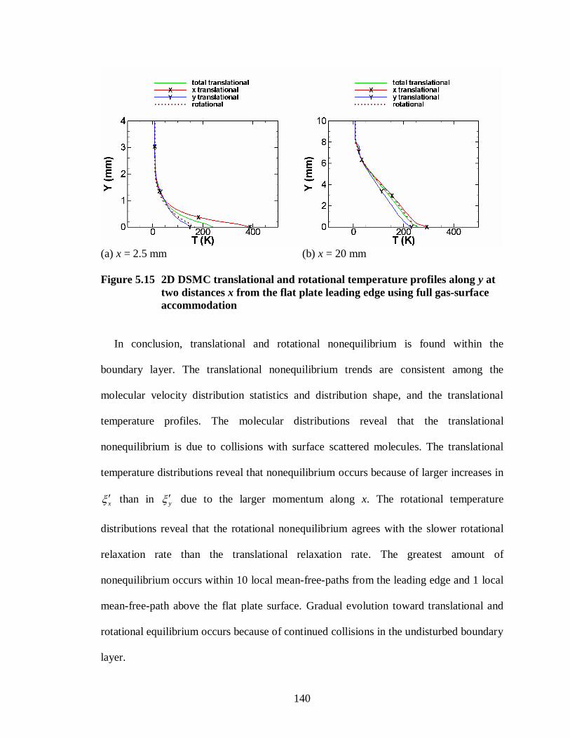
140
(a) x = 2.5 mm (b) x = 20 mm
Figure 5.15 2D DSMC translational and rotational temperature profiles along y at
two distances x from the flat plate leading edge using full gas-surface
accommodation
In conclusion, translational and rotational nonequilibrium is found within the
boundary layer. The translational nonequilibrium trends are consistent among the
molecular velocity distribution statistics and distribution shape, and the translational
temperature profiles. The molecular distributions reveal that the translational
nonequilibrium is due to collisions with surface scattered molecules. The translational
temperature distributions reveal that nonequilibrium occurs because of larger increases in
x than in y due to the larger momentum along x. The rotational temperature
distributions reveal that the rotational nonequilibrium agrees with the slower rotational
relaxation rate than the translational relaxation rate. The greatest amount of
nonequilibrium occurs within 10 local mean-free-paths from the leading edge and 1 local
mean-free-path above the flat plate surface. Gradual evolution toward translational and
rotational equilibrium occurs because of continued collisions in the undisturbed boundary
layer.

141
5.6 Apollo 6 Flight Simulations Using the Two Models
The assessment of the Maxwell and CLL gas-surface interaction models by
simulations of a flat plate windtunnel test enabled detailed, relatively inexpensive
analysis and satisfactory comparison with real physical data. The assessment of the two
models is completed here by applying them to a spaceflight application. The simulation
set-up for the Apollo 6, 110 km entry trajectory point, provides an adequate framework
for fulfilling this final part of the assessment. Therefore, the basic conditions described in
Section 4.2 are employed. The isothermal wall condition defined in Section 4.3, which
was determined to be adequate in Chapter 4, is selected. Case 3 of table 4.3 is repeated,
forming two additional cases, denoted as cases 6 and 7, where the optimum values of aM
and t found from the flat plate simulations are selected to place a connection with these
simulations. Table 5.8 summarizes the two Apollo 6 flight simulation cases. In case 6, the
levels of rotational and vibrational energy accommodation are equal and represented by
the internal energy accommodation coefficient aE_int. This coefficient is set equal to the
Maxwell accommodation coefficient aM, which governs the translational mode of
molecular thermal energy. In case 7, aE_int carries the same definition, however, in
conjunction with the CLL model. The size of each simulation case is the same as listed in
Table 4.2, in Chapter 4; however, in these cases, double the number of processors, 32
instead of 16, was used, resulting in nearly half the simulation time. The parallel
efficiency of case 6 is about 98% based on the 16 processor runtime of 15 hr. The
simulation wall time spent by each simulation is listed in Table 5.8. These wall times
show that numerical expense of the CLL model is similar to that of the Maxwell model.

142
Note, because the wall times are dependent on the parallel computing system’s
communication efficiency during the time of simulation, these times are representative.
Table 5.8 Apollo 6 flight simulation cases for assessing the two gas-surface
interaction models using the isothermal wall temperature, Tw,i = 830 K
Case Gas-surface interaction model and accommodation Simulation wall time
6 Maxwell, aM = 0.875, aE_int = 0.875 7.68 hr
7 CLL, t = 0.875, n = 1.000, aE_int = 0.875 7.29 hr
The assessment of the gas-surface interaction models using space capsule reentry
simulations begins with an examination of the translational temperature contours near the
space capsule. Figures 5.16 (a) and (b) compare the contours that result from using the
Maxwell and CLL gas-surface interaction models. The overall appearance of each
contour plot is similar; however, in the compression region ahead of the vehicle, lower
translational temperatures result from the CLL model. The changes in the peak
(a) Case 6 (Maxwell) (b) Case 7 (CLL)
Figure 5.16 Contour plots of translational temperature at symmetry surface of
three-dimensional Apollo 6 flight simulations using the Maxwell and
CLL gas-surface interaction models

143
translational temperatures, as well as in the peak rotational and vibrational temperatures,
are listed numerically in Table 5.9. There are slight effects on the peak field temperatures
as a consequence of switching the gas-surface interaction model.
Table 5.9 Effects of gas-surface interaction models on maximum field
temperatures found within compression region (K)
Case Translational Rotational Vibrational
6 (Maxwell) 40,342 5,898 2,295
7 (CLL) 36,900 5,581 2,154
Increase – 8.5 % – 5.3 % – 6.1 %
The differences in the peak field temperatures in the compression region are due to
differences in the way each gas-surface interaction model scatters molecules. These
differences are indicated by Figs. 5.17 (a) and (b), which are scattering plots from the flat
plate windtunnel test simulations associated with aM and t = 87.5%. The plots are of the
non-normalized probability distributions. They indicate that the Maxwell model results in
(a) x = 0 mm (b) x = 5.0 mm
Figure 5.17 2D DSMC probability distributions of scattering angle at two locations
on flat-plate surface, y = 0 mm, from windtunnel test simulations using
aM and t = 87.5%

144
greater backscatter, and thus, causes a wave of more energetic inter-gas collisions in the
near field and the greater peak field temperatures in the compression region.
The assessment using these flight simulations concludes with an examination of the
aerodynamics and surface heating. The associated data are listed in Table 5.10. Switching
the gas-surface interaction models slightly affects drag and pitching moment. The
pressure contribution to the pitching moment is slightly decreased and affected slightly
more than the shear contribution. These contributions destructively interfere. Lift and
Stanton number are affected to a much greater extent. The pressure and shear components
of lift constructively interfere. Each is decreased to a similar extent. The range of effects
is caused by the various differences in the gas-surface interaction models. Any one of
these differences does not appear to stand out. These results further demonstrate the
sensitivity of rarefied aerothermodynamic analysis to gas-surface interaction model; and
thus, the merit of having the correct gas-surface interaction model for these conditions.
Table 5.10 Effects of gas-surface interaction models on aerodynamics and surface
heating
Case CD CL L/D CMO Stmax
6 (Maxwell) 1.68 0.266 0.158 0.113 0.746 pressure* 1.40 0.528 0.091 shear 0.28 –0.261 0.021
7 (CLL) 1.66 0.233 0.140 0.110 0.852 pressure 1.35 0.513 0.086 shear 0.31 –0.280 0.024
Increase (%) – 1.4 – 12.5 – 11.3 – 2.6 14.3 pressure –2.8 –5.5 –5.0 shear 1.4 –6.9 2.4
*pressure and shear components of CD, CL and CMO are listed below the total values, *percentage increases are relative to total values of case 6

145
5.7 Summary and Conclusions
This study began with a review of gas-surface interaction models since the Maxwell
model. The review led to the decision to assess the Maxwell and the CLL gas-surface
interaction models. These are two of the most commonly used models in use with DSMC.
To examine the gas-surface interaction models, computational simulations were made of
an existing windtunnel test study, performed by Cecil and McDaniel (2005), involving a
free jet expansion of nitrogen used to generate rarefied hypersonic flow over a flat plate.
They measured the velocity components, near the flat plate, with planar laser induced
fluorescence (PLIF) of seeded iodine, within a nitrogen flow. A detailed study was made
of the flat plate boundary layer flow, with MONACO simulations employing a
nonuniform inflow condition emulating the windtunnel test.
Prior to embarking on the gas-surface interaction analysis, simulations of the
windtunnel test flow near the flat plate were performed using continuum compressible
boundary layer theory. These simulations demonstrated the necessity of using a kinetic
computational approach to simulate the windtunnel test near equilibrium conditions by
showing large differences in boundary layer velocity and temperature profiles between
the continuum boundary layer theory and the DSMC method. Substantial differences in
skin friction and Stanton number were also revealed between these computational
approaches.
The second part of the DSMC study involved an assessment of the effects of the
different gas-surface interaction models and of varying the gas-surface accommodation
on the flat plate flow simulations. This was done by examining molecular distributions
and boundary layer velocity profiles. For molecular velocity distributions, the Maxwell

146
and CLL gas-surface interaction models gave similar x distributions, but distinct y
distributions, at partial levels of gas-surface accommodation. In addition, scattering
distributions were examined. The Maxwell model resulted in distributions with
unrealistic peaks due to specular reflection; whereas, the CLL model resulted in petal-
shaped distributions, similar to observations of molecular beam studies, reported in the
literature. Moreover, while the Maxwell scattering distributions experienced abrupt
changes with increasing accommodation and position, the CLL distributions varied
smoothly. Hence, for no significant additional cost, the CLL model gave more realistic
scattering distributions. For boundary layer velocity profiles, the computed set of profiles
encompassed the PLIF data, except for x > 12.5 mm, where an adverse pressure gradient
appeared due to windtunnel test flow phenomena outside the specified computational
domain. The Maxwell and CLL models gave the same boundary layer profiles at 50 to
100% gas-surface accommodation, based on Maxwell’s fraction and CLL’s tangential
momentum accommodation coefficient. Finally, 90% gas-surface accommodation
yielded the overall best agreement between the simulations and the PLIF data; this result
is consistent with physical reasoning and the general trends found in the literature.
The study continued by examining the effects of the seeded iodine in the windtunnel
tests. The corresponding DSMC computations were an order of magnitude more
expensive than the pure nitrogen computations because the iodine mean-free-path was an
order of magnitude smaller than the nitrogen mean-free-path due to the larger molecular
weight and collision cross section of the iodine. The iodine velocity was very similar to
the nitrogen velocity field, as expected from the ~10–4
mixture ratio of iodine to nitrogen.
Differences in the profiles are mainly due to the larger inertia of the seeded iodine and

147
partly explain differences in the pure nitrogen simulations and windtunnel test
measurements. Because the overall differences are slight, the seeded iodine simulation
affirms the pure nitrogen simulations and accredits the PLIF measurement procedure.
The fourth part of the study was an analysis of thermal nonequilibrium in the flow
field. Translational and rotational nonequilibrium is found within the boundary layer. The
translational nonequilibrium trends are consistent among the molecular velocity
distribution statistics and distribution shape, and the translational temperature profiles.
The molecular distributions reveal that the translational nonequilibrium is due to
collisions with surface scattered molecules. The translational temperature distributions
reveal that translational nonequilibrium occurs because of larger increases in random
molecular speed parallel to the flat plate x than random molecular speed perpendicular
to the flat plate y due to the larger momentum along the direction x parallel to the flat
plate. The rotational temperature distributions reveal that the rotational nonequilibrium is
consistent with the slower rotational relaxation rate than the translational relaxation rate.
The greatest amount of nonequilibrium occurs within 10 mean-free-paths from the
leading edge and 1 mean-free-path above the flat plate surface. Gradual evolution toward
translational and rotational equilibrium occurs because of continued collisions in the
undisturbed boundary layer.
The study concluded with an assessment of the gas-surface interaction models using
Apollo 6 flight simulations. The simulations involved the conditions presented in Chapter
4 and the optimum Maxwell and CLL interaction parameters determined in Section 5.5.5.
Maximum field temperatures and vehicle aerothermodynamic properties were examined.
Significant differences between the simulations using the Maxwell and CLL models were

148
observed for the field temperatures, lift and Stanton number. These results further
demonstrated the sensitivity of rarefied aerothermodynamic analysis to the gas-surface
interaction model; and thus, the merit of having the correct gas-surface interaction model
for these conditions.
149
CHAPTER VI
GENERAL SUMMARY AND FUTURE WORK
6.1 Overview
Motivated by escalating efforts to advance space transportation, computational
simulation capabilities for rarefied and hypersonic flight conditions are becoming
increasingly relevant. Among the few classes of computational approaches for examining
rarefied gas dynamics, the most widely used approach, for spatial scales relevant to
suborbital spaceflight, is the direct simulation Monte Carlo (DSMC) method. Although
the DSMC method has been under development for over forty years, there are still many
areas where improvements can be made. In the search for a definitive thesis goal and as a
consequence of the analysis tools developed for achieving this goal, several aspects of
DSMC analysis were examined beginning from the analysis of aerodynamic coefficients
and culminating with the assessment of gas-surface interaction models, the associated
numerical models of interactions between gas molecules and solid surfaces. To finalize
this dissertation, the major results and conclusions are summarized here and suggestions
for future work related to this research are proposed.

150
6.2 Summary of Results and Conclusions
In Chapter 3, the aerodynamic properties of drag, lift, pitching moment, and lift-to-
drag ratio, of entry vehicle windtunnel test models within a hypersonic, rarefied nitrogen
gas environment were analyzed using three-dimensional DSMC computations. Modified
Newtonian and free molecular flow models were used to develop procedures to compute
the aerodynamic properties computed by the MONACO DSMC code. The aerodynamic
analysis procedures were applied to three dimensional simulations of windtunnel tests of
a blunted cone and a small scale model of the Apollo Command Module. Good
agreement was found between the measured and DSMC data of a blunted cone; however,
this was not the case for the Apollo Command Module. Consequently, the possibility of
discrepant Apollo windtunnel test measurements was examined by additional
axisymmetric simulation studies. These simulations determined that freestream Mach
number and reservoir conditions were measured with sufficient accuracy and that the test
section flow could have been affected by windtunnel wall boundary layer interference.
However, simulations including the windtunnel wall boundary are not possible because
the available references [Potter et al. (1964), Potter et al. (1962)] do not provide
sufficient details of the windtunnel geometry. In conclusion, aerodynamic integration
procedures were validated and a sensitivity study suggested that the 1960’s windtunnel
results of the ACM are potentially affected by wall boundary layer interference, and have
not been further analyzed in this thesis.
In Chapter 4, a sensitivity study was executed on the aerothermodynamics of the
Apollo Command Module (ACM) at the 110 km entry trajectory point of the Apollo 6
mission. The study examined the significance of three physical mechanisms: gas-surface

151
accommodation, surface radiation and flow chemistry. To evaluate the effects of the
changes in these physical mechanisms, Mach number contours, temperature contours,
peak field temperatures, surface heating and aerodynamic coefficients were monitored.
The first two mechanisms were examined by four simulation cases entailing two gas-
surface accommodation conditions and two surface temperature conditions. To examine
the sensitivity of the aerothermodynamics to flow chemistry, one of the inert simulations
was rerun with MONACO chemistry procedures activated. The sensitivity study of the
110 km entry trajectory point of the Apollo 6 revealed that: changes in the gas-surface
thermal accommodation significantly affect the aerothermodynamics; the addition of
surface radiative equilibrium does not significantly affect the aerothermodynamics; and
the inclusion of chemistry does not significantly affect the aerothermodynamics. Thus,
because of the significance of gas-surface interactions found under these reentry
conditions and because the behavior of gas-surface interactions under rarefied hypersonic
conditions is not well understood, the research in this thesis was directed toward
improving the understanding and simulation of gas-surface interactions under hypersonic
rarefied conditions.
Chapter 5 began with a review of gas-surface interaction models since Maxwell. The
review led to the decision to assess the Maxwell and the CLL gas-surface interaction
models, which are two of the most commonly used models in use with DSMC. To
examine the gas-surface interaction models, computational simulations were made of an
existing windtunnel test study, performed by Cecil and McDaniel (2005), involving a free
jet expansion of nitrogen used to generate rarefied hypersonic flow over a flat plate. They

152
measured the velocity components, near the flat plate, with planar laser induced
fluorescence (PLIF) of seeded iodine, within a nitrogen flow.
A detailed study was made of the flat plate boundary layer flow, with MONACO
simulations employing a nonuniform inflow condition emulating the windtunnel test. The
study provided a detailed understanding of the effects of gas-surface interactions and
seeded iodine on the velocity field, and of the thermal nonequilibrium within the
boundary layer. First, 2D DSMC simulations provided good agreement with PLIF
windtunnel test boundary layer velocity profiles, using a proper specification of gas-
surface accommodation, with either the Maxwell or the CLL gas-surface interaction
model; however, the CLL model is physically more realistic and has little additional
computational expense. Second, the seeded iodine simulations affirmed the pure nitrogen
simulations and the PLIF measurement procedures. Third, significant translational and
rotational nonequilibrium near the surface and near the leading edge of the flat plate was
found by observations of molecular velocity distribution statistics and distribution shape
and by observations of translational and rotational temperature profiles. The molecular
distributions revealed that the translational nonequilibrium was due to collisions with
surface scattered molecules. The translational temperature distributions revealed that
translational nonequilibrium occurred because of larger increases in random molecular
speed parallel to the flat plate than random molecular speed perpendicular to the flat plate
due to the larger momentum along the direction parallel to the flat plate. The rotational
temperature distributions revealed that the rotational nonequilibrium was consistent with
the slower rotational relaxation rate than the translational relaxation rate.
153
To conclude the assessment of the gas-surface interaction models, the Apollo 6 reentry
condition at 110 km was revisited. Maximum field temperatures and vehicle
aerothermodynamic properties were examined. Significant differences between the
simulations using the Maxwell and CLL models were observed for the field temperatures,
lift and Stanton number. These results further demonstrated the sensitivity of rarefied
aerothermodynamic analysis to gas-surface interaction model; and thus, the merit of
having the correct gas-surface interaction model for these conditions.
6.3 Suggestions for Future Work
The work presented in this thesis enlightened various areas for further research related
to the computational simulation of transitional and rarefied gas dynamics experienced by
spaceflight. Three general categories have been identified where further work can be
made: program processing, gas-surface interactions and simulation studies involving
comparisons with real physical data. Efforts that will provide progress in each of these
areas are proposed here.
6.3.1 Program processing
To improve the program processing, two projects have been identified. These projects
fall under the subcategories of parallel domain decomposition and grid generation. These
may or may not be particular to the MONACO DSMC code. Currently, the parallel
domain decomposition automatically assigns computational mesh regions to computer
processors based on the number of simulation molecules in order to balance the load of
simulation molecules among the processors. However, this single criterion does not
minimize the communication load between processors. Consider a parallel simulation,

154
involving two processors, of a uniform gas flow through a right circular cylindrical
computational mesh, as shown in Fig. 6.1 (a). The current criterion allows for the
possibility of partition boundaries cutting through regions of large number flux between
partitions, as shown in Fig. 6.1 (b). The large number flux leads to a large communication
overhead between processors. The communication between processors can be reduced by
optimizing the placement of partition boundaries such that the number flux between
partitions is minimized throughout the computational domain. With the additional
criterion, the partition boundaries in the example case would slice through the
computational domain streamwise to the flow and parallel to the cylindrical wall, instead
of across the flow streamlines and perpendicular to the cylindrical walls, as shown in Fig.
6.1 (c). In this case, if the freestream velocity V is much greater than the freestream
most probable molecular speed ,mp , then the streamwise partitioning scheme would
(a) Basic geometry (b) Crosswise partitioning (c) Streamwise partitioning
Figure 6.1 Partitioning scheme for a parallel simulation involving two processors
for a uniform flow traversing a right circular cylindrical domain
V V V

155
reduce the communication, provided that the total number flux across the interprocessor
partition boundary for the streamwise partitioning scheme is less than for the crosswise
scheme. This condition is generally met for rarefied hypersonic flow simulations; hence,
minimizing communication based on number flux is applicable for DSMC simulations of
rarefied hypersonic flow.
Regarding grid generation, there are three projects that can be addressed. These
automatic grid adaptation, the degree of adaptation and automatic moving grid
boundaries. As discussed in Chapter 2, the grid adaptation for the simulations reported in
this thesis was performed manually. Manual adaptation was performed for the two-
dimensional grids to avoid unpredictable convergence roadblocks with an in-house grid
adaptation code when used with general geometries. Manual adaptation was performed
for the three-dimensional grids because no three-dimensional grid adaptation code is
available within the research group. Automatic grid adaptation reduces simulation set-up
time and can result in better grid adaptation, particularly, for three-dimensional grids.
Consequently, it is recommended that automatic grid adaptation capabilities be developed
for two and three dimensional grids based on a more robust grid generation code than the
presently available in-house grid generation code.
The degree of adaptation in DSMC is based on the criterion discussed in Chapter 2
that the computational cell size be no larger than the local-mean-free path. In regions of
large macroscopic gradients, Bird (1994) generally recommends s < / 3 and t << .
Statistically this is sufficient. However, to satisfy any doubts it would be interesting to
test whether further refinements produce any differences in the aerodynamic results of

156
windtunnel test or flight simulations. In this spirit, one may also perform sensitivity
studies regarding the number of simulation molecules and the frequency of sampling.
Automatic moving grid boundaries are desired for simplifying grid generation for
studies involving several slightly distinct simulations, such as multiple simulations of a
flight vehicle at varying angle-of-attack. The angle-of-attack study would involve an
initial domain boundary configuration, with the vehicle at zero angle-of-attack. Then, the
vehicle surface would be rotated by a desired increment and the computational cells
would be regenerated with a default pattern to provide initial results for grid adaptation
for a second simulation, if necessary. This procedure could also be extended to simulate
vehicle movements for dynamic stability studies.
6.3.2 Gas-surface interaction modeling
Six projects have been identified to improve the understanding and modeling of gas-
surface interactions. First, the visualization of scattering distributions can be extended to
three-dimensions. In order to do this with the MONACO DSMC code, the procedures to
extract probability distributions must be modified to work for three-dimensional
simulations because they currently only work with two dimensional simulations. This
modification would also enable the visualization of three dimensional molecular velocity
distributions. Second, the velocity extraction procedures can be extended to include the
extraction of temperature and internal energy components. This would enable the
visualization of temperature and energy distributions at specified points in space or along
a solid surface for incident and reflected molecules. Third, the CLL model implemented
into MONACO is the basic form. Extensions to this form are available [Lord (1991 and
1995)] and would enable additional case studies about the CLL model. These extensions

157
involve a broader range of translational energy accommodation conditions, rotational
energy accommodation according to the form of the CL kernel, and vibrational energy
accommodation according to a modified form of the CL kernel, which describes a
discrete energy distribution. Fourth, an investigation on nonuniform distributions of gas-
surface accommodation may lead to better agreement between DSMC and windtunnel
boundary layer velocity profiles at all positions over the surface of interest. Fifth, existing
gas-surface interaction models can be modified to handle the variation of accommodation
with surface temperature or a new model can be introduced that inherently has this
flexibility. Finally, existing gas-surface interaction models can be modified to handle the
variation of accommodation with other surface properties, such as surface roughness and
mean molecular spacing, or a new model can be introduced that inherently has these
flexibilities.
6.3.3 Simulation studies involving comparisons with real physical data
The aerodynamic analysis studies of Chapter 3 serendipitously brought to attention
potential errors in some of the hypersonic windtunnel test data from the 1960s. It is
recommended that additional aerodynamic simulation analysis studies be performed
when new rarefied hypersonic windtunnel test data of this kind becomes available. It is
desired that extensive windtunnel geometry and flow conditions be acquired to enable
comprehensive numerical simulation of the entire windtunnel test section.
Gas-surface interaction simulation studies would benefit from additional simple model
configurations such as the flat plate study of Cecil and McDaniel (2005); see also Seldon
et al. (2007). The flat plate windtunnel tests described in Chapter 5 provided field
velocity data; however, field temperature data was not available, at least at the time when
158
the analysis was performed. Hence, it is desired to acquire field temperature laboratory
data to also perform parametric studies involving the variation of boundary layer
temperature profiles with gas-surface accommodation. In addition, it is desired to access
velocity and temperature and/or energy molecular probability distribution data from
future laboratory experiments. For gas-surface interaction modeling, it is particularly
helpful to have available surface scattering probability distributions of velocity,
temperature and energy. This would enable the most direct assessment of probability
based gas-surface interaction models.
Gas-surface interaction simulation studies would also benefit from rarefied flight data
programs. The Apollo 6 flight simulations in Chapters 4 and 5 involved a trajectory point
suitable for a sensitivity study involving changes to physical models in the DSMC
simulation. There are few public documents containing reentry trajectory data sufficient
to produce a DSMC simulation. As usual, the Apollo 6 documents provided no
aerodynamic flight data throughout the rarefied portion of the entry trajectory. Hence,
data from other suborbital flight data collection programs are necessary in order to make
comparisons between flight data and DSMC simulations using various gas-surface
interaction conditions. Along with the benefit to Earth atmosphere spacecraft design,
these comparisons are a step toward improving prediction capabilities of spaceflight near
general atmosphere compositions. With continued exploration efforts to extraterrestrial
atmospheres, such as the Martian atmosphere, the studies must be extended to incorporate
the gas compositions of these atmospheres. Studies such as these would likely provide
unique information or at least provide a check on similar studies performed elsewhere.

159
BIBLIOGRAPHY

160
BIBLIOGRAPHY
A. A. Agbormbai. A Statistical Theory for Gas Surface Interactions in Rarefied
Hypersonic Flows. I.C. Aero Report 88–01, Imperial College of Science and
Technology, London, 1988.
A. A. Agbormbai. Reciprocity Theory of Vibrationally Excited Many-Body Gas Surface
Interactions. 35th
AIAA Thermophysics Conference, AIAA Paper 2001-2964,
American Institute of Aeronautics and Astronautics, Reston, Virginia, 2001.
B. J. Alder and T. E. Wainwright. Molecular Dynamics by Electronic Computers.
Proceedings of the International Symposium on Transport Processes in Statistical
Mechanics, edited by I. Prigogine, Interscience Publishers, New York, pages 97–131,
1958.
D. A. Anderson, J. C. Tannehill and R. H. Pletcher. Computational Fluid Mechanics and
Heat Transfer. McGraw-Hill Book Company, New York, 1984.
J. D. Anderson. Hypersonic and High Temperature Gas Dynamics. McGraw-Hill Book
Company, New York, 1989.
J. J. Bertin. Hypersonic Aerothermodynamics. American Institute of Aeronautics and
Astronautics, Washington, District of Columbia, 1994.
G. A. Bird. Approach to Translational Equilibrium in a Rigid Sphere Gas. Physics of
Fluids, 6:1518–1519, 1963.
G. A. Bird. Monte Carlo Simulation of Gas Flows. Annual Review of Fluid Mechanics,
10:11–31, 1978.
G. A. Bird. Simulation of Multi-Dimensional and Chemically Reacting Flows.
Proceedings of the 11th
International Symposium on Rarefied Gas Dynamics, edited
by R. Campargue, Commissariat a L’Energie Atomique, Paris, 1979.
G. A. Bird. Monte Carlo Simulation in an Engineering Context. Progress in Aeronautics
and Astronautics, Vol. 74, edited by S. S. Fisher, American Institute of Aeronautics
and Astronautics, New York, pages 239–255, 1981.
161
G. A. Bird. Molecular Gas Dynamics and the Direct Simulation of Gas Flows. Clarendon
Press, Oxford, 1994.
G. A. Bird. Forty Years of DSMC, and Now? Proceedings of the 22nd
International
Symposium on Rarefied Gas Dynamics, edited by T. J. Bartel and M. A. Gallis,
American Institute of Physics, Melville, New York, pages 372–380, 2001.
G. A. Bird. The DS2V/3V Program Suite for DSMC Calculations. Proceedings of the
24th
International Symposium on Rarefied Gas Dynamics, edited by M. Capitelli,
American Institute of Physics, Melville, New York, pages 541–546, 2005.
P. Bond. The Continuing Story of the International Space Station. Springer, New York,
2002.
L. Borgnakke and P. S. Larsen.Statistical Collision Model for Monte Carlo Simulation of
Polyatomic Gas Mixture. Journal of Computational Physics, 18:405–420, 1975.
I. D. Boyd, G. C. Pham-Van-Diep and E. P. Muntz. Monte Carlo Computation of
Nonequilibrium Flow in a Hypersonic Iodine Wind Tunnel. AIAA Journal, 32(5):964–
970, 1994.
D. E. Boylan and B. J. Griffith. Simulation of the Apollo Command Module at Re-entry
Altitudes. Proceedings of the 3rd National Conference on Aerospace Meteorology,
American Meteorological Society, Boston, pages 370–378, 1968.
D. E. Boylan and J. L. Potter. Aerodynamics of Typical Lifting Bodies under Conditions
Simulating Very High Altitudes. AIAA Journal, 5:226–232, 1967.
J. L. Brown. Turbulence Model Validation for Hypersonic Flows. 8th
AIAA/ASME Joint
Thermosphysics and Heat Transfer Conference, Institute of Aeronautics and
Astronautics, Reston, Virginia, 2002.
J. M. Burt. Monte Carlo Simulation of Solid Rocket Plumes at High Altitude. Dissertation
for Ph.D. (Aerospace Engineering), University of Michigan, Ann Arbor, 2006.
J. M. Burt. Post doctoral work, University of Michigan, Nov. 2006.
J. M. Burt and I. D. Boyd. Evaluation of a Particle Method for the Ellipsoidal Statistical
Bhatnagar-Gross-Krook Equation. AIAA Paper 2006-989, 44th
AIAA Aerospace
Sciences Meeting and Exhibit, American Institute of Aeronautics and Astronautics,
Reston, Virginia, 2006.
P. Butterworth-Hayes. Space Tourism Race Speeds Up. Aerospace America, 45(8):4–6,
2007.
C. Cai. Private communication, March 2005.

162
F. Cajori. Sir Isaac Newton’s Mathematical Principles of Natural Philosophy and His
System of the World. University of California Press, Berkeley, 1934.
P. Cazin. French Space Plane Research, from Hermes to Transatmospheric Vehicles.
AIAA Paper 89-5020, 1st AIAA National Aerospace Plane Conference, American
Institute of Aeronautics and Astronautics, Washington, District of Columbia, 1989.
D. E. Cecil and J. C. McDaniel. Private communication, March 2007.
D. E. Cecil and J. C. McDaniel. Planar Velocity and Temperature Measurements in
Rarefied Hypersonic Flow Using Iodine LIF. 38th
AIAA Thermophysics Conference,
AIAA Paper 2005-4695, American Institute of Aeronautics and Astronautics, Reston,
Virginia, 2005.
C. Cercignani. Boundary Value Problems in Linearized Kinetic Theory. SIAM-AMS
Proceedings, Vol. 1, edited by R. Bellman, G. Birkhoff, and I. Abu-Shumays,
American Mathematical Society, Providence, Rhode Island, pages 249–268, 1969.
C. Cercignani. Scattering Kernels for Gas-Surface Interactions. Transport Theory and
Statistical Physics, 2(1):27–53, 1972.
C. Cercignani. Rarefied Gas Dynamics From Basic Concepts to Actual Calculations.
Cambridge University Press, Cambridge, England, 2000.
C. Cercignani and A. Frezzotti. Numerical Simulations of Supersonic Rarefied Gas Flows
Past a Flat Plate: Effects of the Gas-Surface Interaction Model on the Flowfield.
Progress in Aeronautics and Astronautics, Vol. 118, edited by E. P. Muntz, D. P.
Weaver and D. H. Campbell, American Institute of Aeronautics and Astronautics,
Washington, District of Columbia, pages 552–566, 1989.
C. Cercignani and M. Lampis. Kinetic Models for Gas-Surface Interactions. Transport
Theory and Statistical Physics, 1(2):101–114, 1971.
C. Cercignani and M. Lampis. New Scattering Kernel for Gas-Surface Interaction. AIAA
Journal, 35(6):1000–1011, 1997.
C. Cercignani, M. Lampis and A. Lentati. A New Scattering Kernel in Kinetic Theory of
Gases. Transport Theory and Statistical Physics, 24(9):1319–1336, 1995.
P. E. Ceruzzi. A History of Modern Computing. 2nd
Edition, The MIT Press, Cambridge,
Massachusetts, 2003.
S. Chandrasekhar. Newton’s Principia for the Common Reader. Oxford University Press,
New York, 1995.

163
R. Chen, R. K. Argawal, F. G. Cheremisin and Y. Bondar. A Comparative Study of
Navier-Stokes, Burnett, DSMC, and Boltzmann Solutions for Hypersonic Flow Past 2-
D Bodies. AIAA Paper 2007-205, 45th AIAA Aerospace Sciences Meeting and Exhibit,
American Institute of Aeronautics and Astronautics, Reston, Virginia, 2007.
H. K. Cheng. Perspectives on Hypersonic Viscous Flow Research. Annual Review of
Fluid Mechanics, 25:455–484, 1993.
H. K. Cheng and G. Emanuel. Perspective on Hypersonic Nonequilibrium Flow. AIAA
Journal, 33(3):385–400, 1995.
P. Collins. The Coming Space Industry Revolution and Its Potential Global Impact.
Journal of Space Technology and Science, 6(2):21–33, 1990.
S. R. Cook, M. A. Hoffbauer and J. B. Cross. Generating velocity and angular
distribution functions of molecules scattered off of surfaces from measurements of
forces exerted on surfaces by incident gases. 19th
AIAA Advanced Measurement and
Ground Testing Technology Conference, AIAA Paper 96–2227, American Institute of
Aeronautics and Astronautics, Reston, Virginia, 1996.
S. F. de Córdoba. 100 km. Altitude Boundary for Astronautics…,
http://www.fai.org:81/astronautics/100km.asp, 2004.
P. Coue. The Beginning of Hermes Spaceplane (1976-1985). 54th
International
Astronautical Congress, IAC-03-IAA.2.P.02, International Astronautical Federation,
Paris, France, 2003.
R. N. Cox. General Characteristics of Hypersonic Flow Fields. Journal of the Royal
Aeronautical Society, 63:503–508, 1959.
R. S. Crowder and J. D. Moote. Apollo Entry Aerodynamics. Journal of Spacecraft,
6(3):302–307, 1969.
H. M. Deitel and P. J. Deitel. C How to Program. Prentice Hall, Upper Saddle River,
New Jersey, 2001.
D. DePasquale, A. C. Charania and J. R. Olds. The Emerging Orbital Space Tourism
Industry: New Insight into Demand and Prospects for Success. AIAA Space 2006
Conference, AIAA Paper 2006-7478, American Institute of Aeronautics and
Astronautics, Reston, Virginia, 2006.
R. W. Detra, N. H. Kemp and F. R. Riddell. Addendum to Heat Transfer to Satellite
Vehicles Reentering the Atmosphere. Jet Propulsion, 27(12):1256–1257, 1957.
S. Dietrich and I. D. Boyd. Scalar and Parallel Optimized Implementation of the Direct
Simulation Monte Carlo Method. Journal of Computational Physics, 126:328–342,
1996.

164
Engineering Village, Elsevier Information, http://www.ei.org, New York, 2007.
P. S. Epstein. On the Air Resistance of Projectiles. Proceedings of the National Academy
of Sciences of the United States of America, 17(9):532–547, 1931.
J. A. Fay and F. R. Riddell. Theory of Stagnation Point Heat Transfer in Dissociated Air.
Journal of the Aeronautical Sciences, 25(2):73–85 and 121, 1958.
Fédération Aéronautique Internationale (FAI). Sporting Code, Section 8 Astronautics,
Switzerland, 2003.
N. C. Freeman. Non-equilibrium Flow of an Ideal Dissociating Gas. Journal of Fluid
Mechanics, 4(4):407–425, 1958.
T. I. Gombosi. Gaskinetic Theory. Cambridge University Press, Cambridge, England,
1994.
B. J. Griffith. Comparison of Data from the Gemini Flights and AEDC-VKF Wind
Tunnels. AIAA 5th
Aerospace Sciences Meeting, AIAA Paper 67-166, American
Institute of Aeronautics and Astronautics, New York, Jan. 1967.
B. J. Griffith. Comparison of Aerodynamic Data from the Gemini Flights and AEDC-
VKF Windtunnels. Journal of Spacecraft, 4(7):919–924, July 1967.
B. J. Griffith and D. E. Boylan. Reynolds and Mach Number Simulation of Apollo and
Gemini Re-entry and Comparison with Flight. Specialists’ Meeting on Hypersonic
Boundary Layers and Flow Fields of the Fluid Dynamics Panel of AGARD, North
Atlantic Treaty Organization, Paris, pages 8-1–8-21, 1968.
K. Grinter. Apollo Program. http://www-pao.ksc.nasa.gov/kscpao/history/apollo/
apollo.htm, 2005.
W. D. Hayes and R. F. Probstein. Hypersonic Flow Theory. Academic Press, New York,
1959.
W. D. Hayes and R. F. Probstein. Hypersonic Flow Theory. 2nd
Edition, Academic Press,
New York, 1966.
B. L. Haas and I. D. Boyd. Models for Direct Monte Carlo Simulation of Coupled
Vibration-Dissociation. Physics of Fluids A, 5(2):478–489, 1993.
S. J. Henderson and J. A. Menart. Adding Chemical Equilibrium to a Parallel,
Unstructured Euler/Navier-Stokes Flow Solver. AIAA Paper 2006-3736, 36th AIAA
Fluid Dynamics Conference and Exhibit, American Institute of Aeronautics and
Astronautics, Reston, Virginia, 2006.

165
T. A. Heppenheimer. The Space Shuttle Decision NASA’s Search for a Reusable Space
Vehicle. NASA SP-4221, National Aeronautics and Space Administration,
Washington, District of Columbia, 1999.
E. R. Hillje. Entry Flight Aerodynamics from Apollo Mission AS-202. NASA TN D-
4185, National Aeronautics and Space Administration, Washington, District of
Columbia, 1967.
E. R. Hillje and R. Savage. Status of Aerodynamic Characteristics of the Apollo Entry
Configuration. AIAA Entry Vehicle Systems and Technology Meeting, AIAA Paper 68-
1143, American Institute of Aeronautics and Astronautics, New York, 1968.
J. J. Hinchen and W. M. Foley. Scattering of Molecular Beams by Metallic Surfaces.
Proceedings of the 4th
International Symposium on Rarefied Gas Dynamics, Vol. 2,
edited by J. H. de Leeuw, Academic Press, New York, pages 505–517,1966.
C. Hirsch. Numerical Computation of Internal and External Flows. 2nd
Edition, Elsevier,
Burlington, Massachusetts, 2007.
F. C. Hurlbut. Two Contrasting Modes for the Description of Wall-Gas Interactions.
Progress in Astronautics and Aeronautics, Vol. 158, edited by B. D. Shizgal and D. P.
Weaver, American Institute of Aeronautics and Astronautics, Washington, District of
Columbia, pages 494–506, 1992.
F. C. Hurlbut and F. S. Sherman. Application of the Nocilla Wall Reflection Model to
Free-Molecule Kinetic Theory. Physics of Fluids, 11(3):486–496, 1968.
HyperMesh. Version 7.0, Altair Engineering Inc., Troy, Michigan, 2004.
M. S. Ivanov and S. F. Gimelshein. Computational Hypersonic Rarefied Flows. Annual
Review of Fluid Mechanics, 30:469–505, 1998.
E. Josyula and W. F. Bailey. Vibration-Dissociation Coupling Using Master Equations in
Nonequilibrium Hypersonic Blunt-Body Flow. Journal of Thermophysics and Heat
Transfer, 15(2): 157–167, 2001.
K. C. Kannenberg and I. D. Boyd. Development of an Object-Oriented Parallel DSMC
Code for Plume Impingement Studies. 30th
AIAA Thermophysics Conference, AIAA
Paper 95-2052, American Institute of Aeronautics and Astronautics, Washington,
District of Columbia, 1995.
B. W. Kernighan and D. M. Ritchie. The C Programming Language. Prentice Hall,
Englewood Cliffs, New Jersey, 1988.
A. D. Ketsdever and E. P. Muntz. Gas-Surface Interaction Model Influence on Predicted
Performance of Microelectromechanical System Resistojet. Journal of Thermophysics
and Heat Transfer, 15(3):302–307, 2001.

166
E. D. Knechtel and W. C. Pitts. Experimental Momentum Accommodation on Metal
Surfaces of Ions Near and Above Earth-Satellite Speeds. Proceedings of the 6th
International Symposium on Rarefied Gas Dynamics, Vol. 2, edited by L. Trilling and
H. Wachman, Academic Press, New York, pages 1257–1278, 1969.
K. Koura and H. Matsumoto. Variable Soft Sphere Molecular Model for Air Species.
Physics of Fluids, 4:1083–1085, 1992.
I. Kuščer. Reciprocity in Scattering of Gas Molecules by Surfaces. Surface Science,
25:225–237, 1971.
D. B. Lee and W. D. Goodrich. The Aerothermodynamic Environment of the Apollo
Command Module During Superorbital Entry. NASA TN D-6792, 1972.
L. Lees. Hypersonic Flow. Proceedings of the 5th International Aeronautical Conference,
Institute of the Aeronautical Sciences, Los Angeles, pages 241–276, 1955.
D. R. Lide, editor. CRC Handbook of Chemistry and Physics, Internet Version 2007 (87th
Edition), <http:/www.hbcpnetbase.com>, Taylor and Francis, Boca Raton, Florida,
2007.
A. Linan and I. Da Riva. Chemical Nonequilibrium Effects in Hypersonic Aerodynamics.
ICAS PAPER 32, 3rd
International Council of the Aeronautical Sciences, Stockholm,
Sweden, 1962.
R. G. Lord. Application of the Cercignani-Lampis Scattering Kernel to Direct Simulation
Monte Carlo Calculations. Proceedings of the 17th International Symposium on
Rarefied Gas Dynamics, edited by A. E. Beylich, VCH, Weinheim, Germany, pages
1427–1433, 1991.
R. G. Lord. Some Extensions to the Cercignani-Lampis Gas-Surface Scattering Kernel.
Physics of Fluids A: Fluid Dynamics, 3(4):706–710, 1991.
R. G. Lord. Some Further Extensions of the Cercignani-Lampis Gas-Surface Interaction
Model. Physics of Fluids, 7(5):1159–1161, 1995.
MathCad 8 Professional. MathSoft Inc., Cambridge, Massachussetts, 1998.
J. C. Maxwell. On Stresses in Rarified Gases Arising from Inequalities of Temperature.
Philosophical Transactions of the Royal Society of London, 170:231–256, 1879.
R. A. Millikan. Coefficients of Slip in Gases and the Law of Reflection of Molecules
from the Surfaces of Solids and Liquids. The Physical Review, 21(3):217–238, 1923.
T. K. Minton, M. Tagawa and G. M. Nathanson. Energy Accommodation in
Hyperthermal Gas-Surface Collisions: Aerobraking in Planetary Atmospheres.
Journal of Spacecraft and Rockets, 41(3):389–396, 2004.

167
K. Moe. Satellite Drag Coefficients at 150 to 500 km. Advances in the Astronautical
Sciences. 119(2):1197–1206, 2005.
K. Moe, M. M. Moe and S. D. Wallace. Improved Satellite Drag Coefficient Calculations
from Orbital Measurements of Energy Accommodation. Journal of Spacecraft and
Rockets, 35(3):266–272, 1998.
J. N. Moss. Private communication, Dec., 2005.
J. N. Moss, C. E. Glass and F. A. Greene. DSMC Simulations of Apollo Capsule
Aerodynamics for Hypersonic Rarefied Conditions. 9th AIAA/ASME Joint
Thermophysics and Heat Transfer Conference, AIAA Paper 2006-3577, American
Institute of Aeronautics and Astronautics, Reston, Virginia, 2006.
Ch. Mundt. Calculation of Hypersonic, Viscous, Non-equilibrium flows around Reentry
Bodies Using a Coupled Boundary Layer/Euler Method. AIAA Paper 92-2856. AIAA
27th
Thermophysics Conference, American Institute of Aeronautics and Astronautics,
Washington, District of Columbia, 1992.
R. D. Neumann. Defining the Aerothermodynamic Methodology. Hypersonics, Volume I:
Defining the Hypersonic Environment, edited by J. J. Bertin, R. Glowinski, and J.
Periaux, Birkäuser Boston, Boston, Massachussetts, 1989.
S. Nocilla. On the Interaction between Stream and Body in Free-Molecule Flow.
Proceedings of the 2nd
International Symposium on Rarefied Gas Dynamics, edited by
L. Talbot, Academic Press, New York, pages 169–208, 1961.
S. Nocilla. The Surface Re-Emission Law in Free Molecule Flow. Proceedings of the 3rd
International Symposium on Rarefied Gas Dynamics, Vol. 2, edited by J. A.
Laurmann, Academic Press, New York, pages 327–346, 1963.
C. Ollivier-Gooch. GRUMMP Version 0.3.0 User’s Guide. Department of Mechanical
Engineering, University of British Columbia, Vancouver, 2005.
E. S. Oran, C. K. Oh and B. Z. Cybyk, Direct Simulation Monte Carlo: Recent Advances
and Applications. Annual Review of Fluid Mechanics, 30:403–441, 1998.
S. Owen. A Survey of Unstructured Mesh Generation Technology.
http://www.andrew.cmu.edu/user/sowen/survey/index.html, 2007.
C. Park. Nonequilibrium Hypersonic Aerothermodynamics. Wiley, New York, 1990.
P. Pesavento. Russian Space Shuttle Projects 1957-1994. Spaceflight, 37:226, 1995.
J. M. Picone, A. E. Hedin, D. P. Drob and A. C. Aikin, NRLMSISE-00 Emperical Model
of the Atmosphere: Statistical Comparisons and Scientific Issues. Journal of
Geophysical Research, 107(A12):SIA 15-1–SIA 15-16, 2002.
168
S. B. Pope. Turbulent Flows. Cambridge University Press, New York, 2000.
J. L. Potter, G. D. Arney Jr., W. H. Carden and M. Kinslow. Gasdynamic Diagnosis of
High-Speed flows Expanded from Plasma States. IEEE Transactions on Nuclear
Science, NS-11(1):145–157, 1964.
J. L. Potter, G. D. Arney Jr., W. H. Carden and M. Kinslow. Irreversible Flow in
Reservoir and Throat Sections of Wind Tunnels with Constricted-Arc Heaters.
Proceedings of AGARD Fluid Dynamics Panel Specialists’ Meeting, AGARDograph
84, Technical Editing and Reproduction Ltd., London, pages 379–412, 1964.
J. L. Potter, M. Kinslow, G. D. Arney Jr. and A. B. Bailey. Initial Results from a Low-
Density Hypersonic Wind Tunnel. Progress in Astronautics and Rocketry: Hypersonic
Flow Research, Vol. 7, edited by F. R. Riddell, Academic Press, New York, pages
599–624, 1962.
A. Poukhov. Russian Aerospace Plane TU-2000. AIAA Paper 93-5055, AIAA/DGLR 5th
International Aerospace Planes and Hypersonics Technologies Conference, American
Institute of Aeronautics and Astronautics, Washington, District of Columbia, 1993.
Pro/ENGINEER Wildfire. Version 2.0, Parametric Technology Coorporation, Needham,
Massachussetts, 2004.
M. J. Quinn. Parallel programming in C with MPI and OpenMP. McGraw-Hill, Boston,
2004.
M. Rasmussen. Hypersonic Flow. Wiley, New York, 1994.
R. Reagan. State of the Union Address, Feb. 4, 1986.
F. Rogier and J. Schneider. A Direct Method for Solving the Boltzmann Equation.
Transport Theory and Statistical Physics, 23(1-3):313–338, 1994.
C. J. Roy and F. G. Blottner. Review and Assessment of Turbulence Models for
Hypersonic Flows: 2D/Axisymmetric Cases. AIAA Paper 2006-713, 44th Aerospace
Sciences Meeting and Exhibit, American Institute of Aeronautics and Astronautics,
Reston, Virginia, 2006.
W. F. N. Santos. Influence of Gas-Surface Interaction on Hypersonic
Aerothermodynamic Performance of Flat-Nose Power-Law Bodies. 44th
AIAA
Aerospace Sciences Meeting and Exhibit, AIAA Paper 2006-1194, American Institute
of Aeronautics and Astronautics, Reston, Virginia, 2006.
L. C. Scalabrin. Private communication, July, 2007.
S. A. Schaaf. Mechanics of Rarefied Gases. Encyclopedia of Physics: Fluid Dynamics II,
Vol. 8, edited by S. Flűgge and C. Truesdell, Springer-Verlag, Berlin, pages 591–624,
1963.

169
S. A. Schaaf and P. L. Chambré. Flow of Rarefied Gases. Princeton University Press,
Princeton, New Jersey, 1961.
R. Schamberg. A New Analytic Representation of Surface Interaction for Hyperthermal
Free-Molecule Flow with Application to Satellite Drag. Proceedings of the Heat
Transfer and Fluid Mechanics Institute, Stanford University Press, Palo Alto,
California, pages 1–14, 1959.
T. E. Schwartzentruber. A Modular Particle-Continuum Numerical Algorithm for
Hypersonic Non-equilibrium Flows. Dissertation for Ph.D. (Aerospace Engineering),
University of Michigan, Ann Arbor, 2007.
T. E. Schwartzentruber, L. C. Scalabrin and I. D. Boyd. A Modular Particle–Continuum
Numerical Method for Hypersonic Non-Equilibrium Gas Flows. Journal of
Computational Physics, 225(1):1159–1174, 2007.
N. Seldon, C. Ngalande, S. Gimelshein and A. Ketsdever. Experimental Compuatational
Observation of Radiometric Forces on a Plate. 39th AIAA Thermophysics Conference,
AIAA Paper 2007-4403, American Institute of Aeronautics and Astronautics, Reston,
Virginia, 2007.
L. H. Sentman. Free Molecule Flow Theory and Its Application to the Determination of
Aerodynamic Forces. LMSC-448514, Lockheed Missiles and Space Co., Sunnyvale,
California, 1961.
F. Sharipov. Application of the Cercignani-Lampis Scattering Kernel to Channel Gas
Flows. Proceedings of the 22nd
International Symposium on Rarefied Gas Dynamics,
edited by T. J. Bartel and M. A. Gallis, American Institute of Physics, Melville, New
York, pages 347–353, 2001.
Q. Sun. Information Preservation Methods for Modeling Micro-Scale Gas Flows.
Dissertation for Ph.D. (Aerospace Engineering), University of Michigan, Ann Arbor,
2003.
Tecplot. Version 10.0, Tecplot Inc., Bellevue, Washington, 2004.
J. F. Thompson. National Grid Project. Computing Systems in Engineering, 3(1–4):393–
399, 1992.
N. Tsuboi and Y. Matsumoto. DSMC Simulation with Gas-Surface Interaction Models in
Hypersonic Rarefied Flow. Proceedings of the 22nd
International Symposium on
Rarefied Gas Dynamics, edited by T. J. Bartel and M. A. Gallis, American Institute of
Physics, Melville, New York, pages 331–338, 2001.
S. Utah and H. Arai. Monte Carlo Simulation of Reentry Flows Based Upon a Three-
Temperature Model. Proceedings of the 23rd
International Symposium on Space
Technology and Science, Vol. 1, Japan Society for Aeronautical and Space Sciences,
Tokyo, pages 1209–1214, 2002.

170
P. Vijayakumar, Q. Sun and I. D. Boyd. Detailed Models of Vibrational-Translational
Energy Exchange for the Direct Simulation Monte Carlo Method. Physics of Fluids,
11(8):2117–2126, 1999.
W. G. Vincenti and C. H. Kruger, Jr. Introduction to Physical Gas Dynamics. Krieger
Publishing Company, Malabar, Florida, 1965.
W. L. Wang. A Hybrid Particle/Continuum Approach for Nonequilibrium Hypersonic
Flows. Dissertation for Ph.D. (Aerospace Engineering), University of Michigan, Ann
Arbor, 2004.
W. L. Wang and I. D. Boyd. Predicting Continuum Breakdown in Hypersonic Viscous
Flows. Physics of Fluids, 15(1):2003.
E. P. Wenaas. Equilibrium Cosine Law and Scattering Symmetry at the Gas-Surface
Interface. The Journal of Chemical Physics, 54(1):376–388, 1971.
F. M. White. Viscous Fluid Flow. 2nd
Edition, McGraw-Hill, New York, 1991.
J. D. Whitfield and B. J. Griffith. Hypersonic Viscous Drag Effects on Blunt Slender
Cones. AIAA Journal, 2(10):1714–1722, 1964.
J. Wilson, editor. The Vision for Space Exploration. National Aeronautics and Space
Administration, http://www.nasa.gov/mission_pages/exploration/main/index.html,
2007.
J.-S. Wu, K.-C. Tseng and C.-H. Kuo. Application of Local Mesh Refinement in the
DSMC Method. Proceedings of the 22nd
International Symposium on Rarefied Gas
Dynamics, edited by T. J. Bartel and M. A. Gallis, American Institute of Physics,
Melville, New York, pages 417–425, 2001.
X PRIZE Foundation. Ansari X PRIZE,
http://www.xprize.org/xprizes/ansari_x_prize.html, Santa Monica, California, 2006.
N. Yamanishi, Y. Matsumoto and K. Shobatake. Multistage Gas-Surface Interaction
Model for the Direct Simulation Monte Carlo Method. Physics of Fluids,
11(11):3540–3552, 1999.
S. M. Yen. Numerical Solution of the Nonlinear Boltzmann Equation for Nonequilibrium
Gas Flow Problems. Annual Review of Fluid Mechanics, 16:67–97, 1984.