assessment of forest biological diversity. a fao … français de pondichéry assessment of forest...
TRANSCRIPT

HAL Id: hal-00373545https://hal.archives-ouvertes.fr/hal-00373545
Submitted on 6 Apr 2009
HAL is a multi-disciplinary open accessarchive for the deposit and dissemination of sci-entific research documents, whether they are pub-lished or not. The documents may come fromteaching and research institutions in France orabroad, or from public or private research centers.
L’archive ouverte pluridisciplinaire HAL, estdestinée au dépôt et à la diffusion de documentsscientifiques de niveau recherche, publiés ou non,émanant des établissements d’enseignement et derecherche français ou étrangers, des laboratoirespublics ou privés.
Assessment of forest biological diversity. A FAO trainingcourse. 1- Lecture notes
François Houllier, R. M. Krishnan, Claire Elouard
To cite this version:François Houllier, R. M. Krishnan, Claire Elouard. Assessment of forest biological diversity. A FAOtraining course. 1- Lecture notes. Institut Français de Pondichéry, pp.102, 1998, Pondy Papers inEcology. <hal-00373545>

PONDY PAPERS IN ECOLOGY
Documents edited by
François Houllier
Rani M. Krishnan
Claire Elouard
INSTITUT FRANÇAIS DE PONDICHÉRY FRENCH INSTITUTE PONDICHERRY
ASSESSMENT OF FOREST BIOLOGICAL DIVERSITY
A FAO TRAINING COURSE
1. LECTURE NOTES

I n s t i t u t f r a n ç a i s d e P o n d i c h é r y
Assessment of forest biological diversity
A FAO training course
1. Lecture notes
Documents edited by François Houllier, Rani M. Krishnan and Claire Elouard
Pondy Papers in Ecology
May 1998

Contents
Contents..................................................................................................................1
Foreword ................................................................................................................3
Scaling diversity estimates - Rani M. Krishnan........................................................7
Introduction ...................................................................................................7 How then do we compare diversity?...............................................................8 References ................................................................................................... 14
Landscape analysis and vegetation mapping - Gérard Bourgeon ............................ 17
Introduction ................................................................................................. 17 The FAO mapping manual viewpoint ........................................................... 17 Some definitions and notions pertaining to geomorphology.......................... 18 What is the contribution of such an analysis to vegetation mapping?............. 21 How to introduce geomorphological analysis
in phytogeographic inventory operations............................................ 31 References ................................................................................................... 33
Interpretation of satellite images for vegetation mapping - B.R. Ramesh.................35
Introduction ................................................................................................. 35 Worked example...........................................................................................36 Limitations................................................................................................... 37 Suggested reading.........................................................................................37
Assessing species richness and diversity at the community level: methodological background - François Houllier, Clémentine Gimaret-Carpentier. .38
Abstract.........................................................................................................38 Introduction ................................................................................................. 39 Sampling strategies: generalities ....................................................................42 Assessment of species richness.....................................................................46 Assessment of species diversity.....................................................................55 References ....................................................................................................60

2 Assessment of forest biological diversity. Lectures notes
Permanents plots as a means to monitoring forest dynamics and biodiversity - François Houllier .............................................................................. 62
Abstract...........................................................................................................62 Introduction ................................................................................................... 62 A statistical point about permanent plots .........................................................63 Monitoring forest dynamics ............................................................................66 Monitoring species diversity ...........................................................................69 Monitoring species richness and diversity ......................................................70 General discussion..........................................................................................71 References......................................................................................................73
Indicators of the biological diversity of forests at the national level: comments on a French experience - François Houllier .............................................74
Abstract ......................................................................................................... 74 Introduction ....................................................................................................75 Forest-oriented indicators ...............................................................................76 Species-oriented indicators..............................................................................80 Policy-and management-oriented indicators ...................................................81 General discussion .........................................................................................83 References......................................................................................................85
Biodiversity assessment and stand structure: setting up of permanent or temporary plots, and parameters to be studied - Claire Elouard and Rani M. Krishnan ...............................................87
Introduction....................................................................................................87 Permanent plots..............................................................................................88 Temporary plots (transects) ............................................................................ 94 Comparison between the different protocols...................................................96 How permanent plots are used to measure temporal changes
in vegetation dynamics ......................................................................... 99 References................................................................................................... 102
Foreword
The last decade has seen major changes in the assessment of forest resources. Going back to the meeting held in Kotka in 1987 (FINNIDA) and to the subsequent reports published by the FAO after it completed the last decennial Forest Resources Assessment (FAO 1993, 1995, 1996), and taking stock of the ongoing discussions in several international fora such as the Commission on Sustainable Development set up after the United Nations Conference on Environment and Development (Rio de Janeiro 1992), it may be observed: - that the standing stock in the forests is not considered any more as being only a timber or biomass resource, but that it is increasingly viewed as one of the compartments in the global biosphere processes (e.g., as a compartment in the global biogeochemical cycle of carbon); - that the concern about deforestation still very much exists, but that it does not only concern the loss in forest area and wood resources but also, more and more, the loss of species (tree species of course, but also other living organisms which are part of the forest ecosystems); - that the growing concern on the erosion of the biological diversity means that all forms of forest degradation —not only deforestation, the most striking one— should be considered and monitored; - that forest resources encompass many products —timber and non timber—, which are necessary to the very subsistance of local populations and are strongly linked to the maintenance of the biological diversity in forests.
Foresters have always been concerned by the renewal and sustainability of forest resources, but the scope of this very word —sustainability— has changed as a consequence of the growing awareness of the society that forest resources are not just simply timber. These changes are being widely discussed in a number of international scientific, technical and political fora (Palmberg-Lerche 1995) and have already led to new policy orientations. It is worth noting that they are gradually becoming visible in the way forest resources are being assessed (e.g., Anon. 1995, Nyyssönen & Ahti 1996): global change, biodiversity and the need to promote a balanced development which takes care of the local populations and their forest resources cannot be ignored anymore by the forest inventorists.

4 Foreword
It is within this general context that the FAO requested the Institut français de Pondichéry (French Institute of Pondicherry, India) to organize a one-month training course on the "Assessment of biological diversity of forest ecosystems". This training course was part of a French funded project implemented by the FAO in Cambodia, Laos and Vietnam with the aim to "Establishment/strengthening of country capacity in planning, assessment and systematic observations of forest resources in South-East Asian countries" (GCP/RAS/157/FRA).
The training course was attended by twelve South-East Asian forest officers (4 from each country) involved in forest inventory operations, either at the national level or on a regional project basis, and an Indian forest officer from the Tamil Nadu Forest Department. It was organized in continuation of a one-week course in Hyderabad where the participants visited the GIS unit at the Andhra Pradesh Forest Department and the Forestry and Ecology Division at the National Remote Sensing Agency.
The academic and practical organization of the training course was coordinated by Dr. Rani M. Krishnan and Dr. Claire Elouard, with the collaboration of staff from the Institut français de Pondichéry (Dr. V.M. Meher-Homji, Dr. G. Bourgeon, Dr. B.R. Ramesh, Dr. S. Darracq, C. Nouguier, Rattnadeep Datta, S. Aravajy, S. Ramalingam, Barathan Ravi, Gopal, Kanagalingam) and of several other people from the Laboratoire de biométrie, génétique et biologie des populations at Lyon (Dr. J.-P. Pascal), the Karnataka Forest Department, the Kerala Forest Research Institute (Peechi), the Forest Survey of India (Bangalore) and the Centre for Ecological Sciences (Indian Institute of Sciences, Bangalore).
The documents contained in this folder are the revised versions of the lecture notes given to the participants in Pondicherry. The form of a folder, rather than a book or a bound report, was chosen to clearly indicate that these documents are still preliminary. It is true that there are many good textbooks on forest mensuration and inventory which have been published in the 70s and 80s (e.g., Loetsch & Haller 1964, Loetsch et at. 1973, Husch 1971, FAO 1981, Duplat & Perrotte 1981). There are also some, but not so many, textbooks on the methods used to assess biological diversity (e.g., Frontier 1982: 416-436, Magurran 1988, Hawksworth 1995). But the former lack the biological and ecological dimensions that are required if we want to estimate "biodiversity" and they essentially focus on the assessment of forest area, timber volume and timber increment, while the latter are very general with more references to bird or insect communities and to marine ecosystems than to forests.
While dealing with biological diversity, the distinction is often made between the different types of diversity. These types refer to spatial scales and levels of organisation. For this training course, the focus was on the species diversity at different scales (within communities, ecosystems, landscapes and regions) and the community and ecosystem diversity (within landscapes and regions) rather than on

Foreword 5
genetic diversity (on this topic, see for example the articles in Boyle & Boontawee 1995).
The task was thus to try to bring together the classical perspective of forest inventories (with its strong emphasis on sampling strategies) and the ecological approach which is more often followed by researchers. We thus had lectures on the definition of biological diversity itself (Drs. J.-P. Pascal and Rani M. Krishnan), on the biological and ecological evolutionary processes which help creating or maintaining diversity (Dr. J.-P. Pascal), on vegetation and forest mapping and the way to include ecofloristic information (Drs. J.-P. Pascal, V.M. Meher-Homji and B.R. Ramesh), on sampling strategies and on the utility of permanent plots (Drs. F. Houllier and C. Elouard).
We also thought that it was necessary to mention the role of human societies, not only by considering the level of migration due to human activities (Dr. P.D. Mahadev) but also by providing an insight into how minor forest products can be quantified and valued (Dr. N. Sasidaran). Indeed, timber and non timber forest products constitute a direct link between the existing biological diversity, the needs and activities of the local population and the social and economic value attached to the maintenance of species and ecosystems.
The lectures were completed by a study tour in Karnataka under the supervision of Drs. C. Elouard and Rani M. Krishnan. This tour provided an opportunity to interact with Indian foresters and scientists and to apply sampling strategies in two contrasted forest ecosystems: a moist evergreen forest (near Makut) and a deciduous forest (near Bandipur). These field case studies were carried out thank to the help and collaboration of the Karnataka Forest Department and the Centre for Ecological Sciences.
The data collected during the field case studies were analysed by the participants at their return in Pondicherry. The aim of this analysis was to understand and practice simple methods by which diversity and richness can be quantified: thus, comparison of methods (plotless vs. plot-based, role of sample size, applicability of various indices) was examined. The report which summarizes the output of these case studies was prepared by Drs. Rani M. Krishnan and C. Elouard, and is presented in the volume 2 (PPE n° 5).
K.D. Singh François Houllier Forest Resources Assessment Project Institut français de Pondkhéry
FAO, Rome India

6 Foreword
References
Anon. 1995. Les indicateurs de gestion durable des forêts françaises. Ministère de l'agriculture et de la pêche, Paris, 49 pp.
Boyle T.J.B., Boontawee B. (Eds). 1995. Measuring and monitoring biodiversity in tropical and temperate forests, CIFOR, Bogor, Indonesia, 395 pp.
Duplat P., Perrotte G. 1983. Inventaire et estimation de l'accroissement des peuplements forestiers. Office National des Forêts, Paris, 432 pp.
FAO. 1981. Manual of forest inventory. FAO Forestry Paper, 27, FAO, Rome, 200 pp.
FAO. 1993. Forest resources assessment 1990. Tropical countries. FAO Forestry Paper, 112, FAO, Rome, 101 pp.
FAO. 1995. Forest resources assessment 1990. Global synthesis. FAO Forestry Paper, 124, FAO, Rome, 44 pp.
FAO. 1996. Forest resources assessment 1990. Survey of tropical forest cover and study of change processes. FAO Forestry Paper, 130, FAO, Rome, 152 pp.
FINNIDA. 1987. Ad hoc FAO/ECE/FINNIDA meeting of experts on forest resource assessment (Helsinki, October 1987).
Frontier S. 1983. Stratégies d'échantillonnage en écologie. Masson, Paris, 494 pp. Hawksworth D.L. (ed.) 1995. Biodiversity. Measurement and estimation. Chapman
& Hall, London, 140 pp. Husch B. 1971. Préparation d'un inventaire forestier. FAO, Rome, 135 pp. Loetsch F., Haller K.E. 1964. Forest inventory. Vol. 1. BLV, München, 2nd ed.,
436 pp. Loetsch F., Haller K.E., Zöhrer F. 1973. Forest inventory. Vol. 2. BLV,
München, 2nd ed., 469 pp. Magurran A.E. 1988. Ecological diversity and its measurement. Croom Helm Ltd,
London, 179 pp. Palmberg-Lerche C. 1994. FAO programmes and activities in support of the
conservation and monitoring of genetic resources and biological diversity in forest ecosystems. In Boyle T.J.B. & Boontawee B. (Eds). 1995. Invited Paper to the Symposium Measuring and monitoring biodiversity in tropical and temperate forests, Chiang Mai, Thaïland (28/8-2/9/94), 15 pp.
Nyyssönen A., Ahti A. 1996. Expert Consultation on Goblal Forest Ressources Assessment 2000. Kotka III. The Finnish Forest Research Institute, Research Papers 620, Helsinki, 369 pp.

Scaling diversity estimates 7
Scaling diversity estimates
Rani M. Krishnan
Introduction
On a very small scale, it is well known that the number and diversity of species increases as we move from the canopy to the understorey conditions (Fig. 1). This is partly due to the size of the organisms encountered in the gradient, and an inverse relationship is possible between size and abundance (Muller-Dombiois et al. 1981).
Layer number
Figure 1. The number of individuals and species of woody plants per hectare in different layers of the canopy of a Hawaiian rain forest. I = herbaceous plant layer (0-0.5 m); II = tree fern layer (> 0.5-5 m); III : low-stature tree layer (> 5-10 m); IV = intermediate-stature tree layer (> 10-15 m); V = emergent layer (> 15 m). (From Mueller-Dombois et al. 1981.)

8 Assessment of forest biodiversity. Lecture notes
This understanding can be applied or extended for calculating the number of same species for a specific number of same sized individuals that would compensate for the bias introduced by sampling plants of different sizes using the same sized plots.
The concept of diversity can be understood and extrapolated to larger scales only by comparisons. For instance, low-diversity tropical forests of Peruvian Amazon, Amazon basin, Mangrove forests and flooded palm forests are compared with the neighbouring species-rich forests. This brings out the importance of the role of other environmental factors and the spatio-temporal scale that determines diversity.
Comparing diversity over different space and time scales involves the use of statistics to interpret diversity. The problem with statistical interpretation of diversity is that although evenness and richness are independent properties, they could give high correlations in samples obtained at random.
How then do we compare diversity?
The most extreme (and the most unacceptable) example for depicting the diversity of an ecosystem would be to sum up the total number of species into a single number. Such a lumping not only ignores the critical biological differences between the groups, guilds and organisms, but also on the whole ignores the different ecological processes that influence each type of organism (Heal & Grime 1991).
Comparisons between organisms or groups of organisms that are of the same 'functional type' is of relevance here. The choice of organisms between the same 'functional type' can therefore provide an understanding of the factors that influence the diversity of the organisms across a larger geographic scale. For example, comparing the birds of North and South America would be misleading if the total number of birds was taken. If the functional type of each continent is studied for all the areas compared, patterns of diversity will emerge. For instance, comparisons between frugivorous, insectivorous, nectarivorous and omnivorous birds would be more useful and meaningful (Huston 1994). This method has been used to compare shrub diversity in the understorey of evergreen tropics globally (Rani & Davidar 1996). Comparing organisms of similar functional types helps understand the factors in the community that regulate the partitioning of diversity into their components.
The basic unit of diversity at smaller scales can be individual species. Lumping of 'functional groups' can provide insights into community organization. Thus, at the community level, trophic, guild and life form diversity are integral parts of the community organization (Fig. 2). The mechanisms that influence diversity at larger scales are different from those that operate within groups of organisms at smaller scales.

Scaling diversity estimates 9
Community species diversity
Figure 2. Causal factors that may influence the species diversity of a community
Selection of an appropriate unit for comparison is therefore a basic and important issue in studying diversity. The time and space scales at which the samples should be collected are also critical, especially due to the comparative nature of the studies. These scales are important not only for organisms, but also for appropriate sampling and interpretion of physical and biological factors that can influence species diversity. Of these, resources which fluctuate on a spatio-temporal scale and climatic conditions, like rainfall and temperature which vary over space and time, are significant. If the area sampled exceeds the size of an environmentally homogeneous area, the relationship between the species and area (expressed as species / area curve) should rise again as species from other environments are sampled. With a species / area curve over larger scales, more complex patterns are likely to appear (Fig. 3).
Species / area curve is used to test the hypothesis that rates of diversity increase with area. The species / area curve should begin from spatially random distribution and level off at the total number of species within the homogeneous area or habitat.

10 Assessment of forest biodiversity. Lecture notes
T1 = Transect 1; T2 = Transect 2; T3 = Transect 3 (Redrawn from Shmida and Wilson 1985)
Figure 3. Increase in plant species diversity with increasing sample area, in the Judean desert of Israel. Transect T1 is in a homogeneous area. T2 is in a heterogeneous area with four vegetation zones and demonstrates a stairstep pattern caused by complete sampling of a single homogeneous habitat followed by sampling in an different habitat. T3 is in a homogeneous area close to transect T2, and shows the presence of species from both the homogeneous and zoned area. (From Shmida and Wilson 1985.)
What are the levels of species diversity?
It is clear from the above that environmental heterogeneity and homogeneity are critical factors in explaining species diversity. The relationship between sampling scale and the processes that influence species diversity forms the basis for distinguishing 'within-habitat diversity' and 'between-habitat diversity'. The 'within-habitat diversity' is also known as alpha diversity (α-diversity). It represents the number of species or other components of species diversity within the area and explains the species homogeneity (Table 1).
'Between-habitat diversity', also known as beta diversity (ß-diversity), is essentially the response of organisms to environmental heterogeneity. It is measured as similarity index or species turn-over rate.
Gamma diversity is the number of species within a region. It can also be defined as the difference in species composition between similar habitats in different geographical areas (Shmida & Wilson 1985, Fig. 3).
Landscape diversity of an area can be expressed as 'mosaic-diversity', in which the species and their habitats tend to be represented in a truly diverse pattern.

Scaling diversity estimates 11
Table 1. Hypotheses explaining the diversity of trees in natural ecosytems
Author Prediction Expected results 1. Static or classical view Whittaker (1977) Co-existing species in a community Local diversity is correlated
share resources among themselves to the environment and and occupy a part of the different diversity of the resources, available habitats.
2.Species diversity MacArthur (1965); Willson 1. Relationship between the niches Diversity thrives in mosaics (1974) 2. Habitat heterogeneity of microsites, varying
3. Trophic equivalence according to environmental attributes and successional staees.
3.Models for explaining tropical tree diversity i) Intermediary disturbance Density of seeds / seedlings Rare species have higher
hypothesis (Connell et decreases with distance from parent recruitment than common al. 1984) (Janzen 1970). species under high predatory
pressure ii) Regeneration niche Diversity is maintained by Diversity higher in sytems
hypothesis (Grubb availability of regeneration niche. with disturbance 1977)
iii) Accidentals or mass Species diversity is inflated by the Constant input of accidentals
effect (Brown & Kodric- presence of accidental species inflates the richness and Brown 1977) (poor adaptors to habitats) inhibits their competitive
exclusion.
What are the major issues on diversity that ecologists are trying to find an answer to?
The fundamental questions that arise when we study and compare diversity are related to the origin and maintenance of diversity. Crucial questions on diversity like: - How is diversity generated? - Why does diversity persist? - Where does diversity thrive? - When does diversity survive? have no simple answers.
How is diversity generated? To answer this question we searched all the species rich ecosystems in the world to try and find the common underlying factors. In general, it can be stated that plant species diversity increases with increase in rainfall and decrease in the length of the dry season (Huston 1988; Ramesh & Pascal 1984).
Phytogeographers are of the opinion that several species present in a given area indicate that they are relicts of the past and that much of the observed diversity is actually a reflection of a common past and subsequent evolution following isolation (Gentry 1988). It is interesting to note that the comparisons in phytogeography begin with families, move down to genera and on to species levels.

12 Assessment of forest biodiversity. Lecture notes
These levels of comparisons are important in understanding the origin and evolution of the flora. The debate on the rates of evolution and extinction, process of succession and role of climate and environment gradients are inconclusive and have not helped much in furthering our understanding of the process of speciation.
Why does diversity persist? In a remarkable experiment, the productivity of an ecosystem was linked to survival and maintenance of diversity (savanna). The results led us to examine the role of productivity and nutrient recycling in the persistence of species diversity (Tilman et al. 1996).
Several models try to explain the persistence of diversity (Table 1). Significantly, these models can explain the role of the ecosystem process at the level of the community only. The role of the landscape in explaining the diversity is yet to be understood wholistically, although they can be readily broken down into their components and the process and interactions studied for each component (Fig. 4).
Where does diversity thrive? When we compare the diversity on a global scale, latitudinal gradients, reverse latitudinal gradients and altitudinal gradients of diversity appear to be important. Diversity of trees increases from the monospecific boreal forests to the mind boggling diversity of tropical rain forests. Diversity of orchids is seen to increase dramatically towards the tropics. This is also true for most plant groups. Increasing diversity with decreasing latitudes has been observed in vertebrates, mammals and birds.
Reverse latitudinal gradients of diversity are seen in fresh water fishes where diversity decreases from the poles towards the tropics. Sea birds also have a higher diversity in the poles than in tropical latitudes. This pattern has also been reported for lichens, marine benthic organisms, parasitic wasps and soil nematodes.
Species diversity generally decreases with increase in elevation. Significant decrease in diversity over altitudes has been observed in vascular plants (Nepalese Himalaya) and birds (New Guinea). Environmental factors like temperature and rainfall are known to create complex patterns with changes in conditions along elevational gradients.
Although diversity is by and large confined to the tropics globally, there are other areas where specific groups have more diversity than in the tropics (Huston 1994).
When does diversity survive? Several theories have been put forward to explain the maintenance of diversity in the tropics. They suggest that diversity can survive only when there is a constant evolution induced by disturbance on different spatial and temporal scales (Table 1).

Scaling diversity estimates 13
Landscape > Ecosystem > Community > Population > Species > Genotypes
Figure 4. Levels of diversity and their applicability (Arranged in order of decreasing complexity)

14 Assessment of forest biodiversity. Lecture notes
References
Barton N.H. 1979. Gene flow past a cline. Heredity, 43 (3): 333-339. Bijlsma R., Ouborg N.J., Van Treuren R. 1991. Genetic and pheonotypic variation
in relation to population size in 2 plant species Salvia pratensis and Scabiosa columbaria. In Seitz A. & Loeschcke V. (Eds): Species conservation: A population-biological approach, Birkhauser Verlag, Switzerland, pp. 89-102.
Brown J.H., Kodric-Brown A. 1977. Turnover rates in insular biogeography: effect of immigration on extinction. Ecology, 58: 445-9.
Connell J.H., Tracy J.C., Webb L.J. 1984. Compensatory recruitment, growth and mortality as maintaining rain forest tree diversity. Ecological monographs, 54: 414-164.
Connell J.H., Tracy J.C., Webb L.J. 1984. Compensatory recruitment, growth and mortality as maintaining rain forest tree diversity. Ecological monographs, 54: 414-164.
Epperson B.K., Allard R.W. 1984. Allozyme analysis of the mating system in lodge pine populations. The Journal of Heredity, 75: 212-214.
Gentry A.H. 1988. Changes in plant community diversity and floristic composition on environmental and geographic gradients. Oikos, 75 (1): 1-34.
Grubb P.J. 1977. Maintenance of species richness in plant communities: the importance of regeneration niche. Biological Review of Cambridge Philosophical Society, 52: 107-145.
Hallé F., Oldeman R.A.A., Tomlinson P.B. 1978. Tropical trees and forest, an architecture analysis. Springer-Verlag.
Hamrick J.L., Muraawski D.A. 1990. The breeding structure of tropical tree populations. Plant species biology, 5: 157-165.
Harvey P.H., Goodfray H.C.J. 1987. How species divide resources. American naturalist, 129: 318-20.
Heal O.W., Grime J.P. 1991. Comparative analysis of ecosystems: Past lessons and future directions. In Cole J., Lovett G., Findlay, S. (Eds.): Comparative analyses of Ecosystems: patterns, mechanisms and theories, Springer- Verlag, New York, pp. 7-23.
Huston M.A. 1994. Biological diversity-The coexistance of species on changing landscapes. Cambridge University Press, New York.
Janzen D.H. 1970. Herbivores and the number of tree species in tropical forests. American Naturalist, 104: 501- 528.
Krebs C.J. 1985. Ecology. Experimental analysis of distribution and abundance. Harper & Row, New York.

Scaling diversity estimates 15
MacArthur R.H. 1965. Patterns of species diversity. Biological Review, 40: 510-33.
Mader H.-J. 1991. The isolation of plant and animal populations: aspects for a European nature conservation strategy. In Seitz A. & Loeschcke V. (Eds): Species conservation: A population-biological approach, Birkhauser Verlag, Switzerland, pp. 265-276.
May R.M. 1981. Patterns in multi-species communities. In May R.M. (Ed.): Theoretical ecology: principles and applications, Blackwell, Oxford, pp. 197-227.
Mayr E. 1970. Populations, species and evolution. The Belknap Press, Cambridge. Muller-Dombois et al. 1981. Altitudinal distribution of organisms along an island
mountain transect. In Muller-Dumbois D.K.W., Bridges Carlson H.L. (Eds.): Island Ecosystems: Biological organization in selected Hawaiian communities. Hutchingson Ross, Pennsylvania, pp. 77-180.
Murawski D.A., Hamrick J.L. 1991. The effect of the density of flowering individuals on the mating systems of nine tropical tree species. Heredity, 67: 167-174.
Murawaski D.A., Hamrick J.L. 1992. The mating system of Cavanillesia platanifolia under extremes of flowering-tree density: A test of predictions. Biotropica, 24 (1): 99-101.
Nicholas S.M. 1986. Gene flow and the measurement of dispersal in plant populations. Journal of Biological education, 20 (1): 61-65.
Palmer J.D., Jansen R.K., Michaels H.J., Chase M.W., Manhart J.R. 1988. Chloroplast DNA variation and plant phylogeny. Annals of Missouri Botanical Garden, 75(4): 1180-1206.
Rani M. Krishnan, Davidar P. 1996. The shrubs of Western Ghats (South India): floristics and status. Journal of Biogeography, 23: 783-789.
Raunkiaer C. 1934. The life-forms of plants and statistical plant geography. Oxford. Schall B.A., Learn B.H. 1988. Ribosomal DNA variation with in and among plant
populations. Annals of Missouri Botanical Garden, 75 (4): 1207-1216. Schuster W.S., Alles D.I., Mitton J.B. 1989. Geneflow in Limber pine: evidence
from pollination, phenology and genetic differenciation along an elevational transect. American Journal of Botany, 76 (9): 1395-1403.
Shmida A., Wilson M.V. 1985. Biological determinants of species diversity. Journal of Biogeography, 12: 1-20.
Southwood T.R.E., Brown V.K., Reader P.M. 1979. Relationship of plant and insect diversities in succession. Biological journal of Linneanean Society, 12: 327-48.
Tilman D. 1988. Plant strategies and the dynamics and structure of plant communities. Princeton university press, New Jersey.
Tilman D., Wedin D, Knops J. 1996. Productivity and sustainability influenced by biodiversity in grassland ecosystems. Nature, 379: 718- 720.

16 Assessment of forest biodiversity. Lecture notes
Whittaker R.H. 1977. Evolution of species diversity in land communities. Evolutionary Biology, 10: 1-67.
Willson M.F. 1974. Avian community organization and habitat structure. Ecology, 55: 1017-29.

Landscape analysis and vegetation mapping 17
Landscape analysis and vegetation mapping
Gérard Bourgeon
Introduction
The aim of this paper is to examine why a touch of geomorphological analysis of landscapes should be introduced in vegetation mapping procedures, and how. A study of the various vegetation maps, including those published recently by this Institute, is sufficient to show that they are not generally based on geomorphological analyses and zoning. Two questions then arise: - What would the introduction of such an analysis give? and, - How to introduce it?
A critical examination of FAO's recommendations ("Classification and Mapping of Vegetation types in Tropical Asia" manual 1989), and a study of a few concrete examples would help answer the first question before giving practical suggestions on how to implement geomorphological analysis.
The FAO mapping manual viewpoint
The authors of the manual Classification and Mapping of Vegetation types in Tropical Asia (FAO ibid.) distinguish two levels in the classification of plant formations: - "the ecological order based on climatic, physiographic or edaphic factors" is "the first level of the classification"; - "the ecofloristic zone for which the dominant or characteristic species of the flora are taken into account" is "the basis of the proposed classification".
The text itself is not very precise regarding the hierarchical relationships between the two levels of the classification, but many examples in the manual show that the ecofloristic zones are distinguished on the basis of bioclimatic and floristic criteria, and that edaphic types intervene only when they express highly specific conditions, e.g., mangroves, peat bogs, etc. The problems linked to the scale and to the change of scale, which are inherent to all cartographic works, are not dealt with. Nevertheless, the authors' choice of scale seems to be only 1/1,000,000 which

18 Assessment of forest biodiversity. Lecture notes
would explain the fact that they did not have to face the problem of changing the scale.
The mapping and classification are not, in fact, based on an explicit analysis of land forms or land systems despite the authors' claims that they are so: "The physiographic contours and the soils help in defining further the bioclimatic limits. The subdivisions of physiographic and edaphic orders are relatively distinct on the terrain; they corrrespond, on the whole, to the notion of land forms and land systems[...]." (FAO ibid. p. 9).
Only the anthropogenic effects have been systematically taken into account to explain the plant formations differing from the "climax" type. The authors of the manual, after emphasizing the necessity of taking land forms and land systems into consideration, seem to have stumble over the second question stated above: how to introduce a land systems analysis.
Moreover, they admit to having difficulties in appreciating the role of soil: "With reference to edaphic formations, if large units of vegetation of unquestionably edaphic origin (such as hygrophytic or halophytic communities) are exempted, the relationships between plant communities and soils are generally not easy to establish..." (FAO ibid. p. 13).
To conclude this brief critical analysis, it can be stated that if foresters have, since a long time, recognized the necessity of taking into consideration criteria such as geomorphology and the nature of the soil for preparing vegetation maps, it would most probably be geomorphologists, and not botanists or plant ecologists, who could provide information on the methods and means of carrying them out.
Some definitions and notions pertaining to geomorphology
Definition of the terms “land system”, "terrain classification" and "land form"
CSIRO (Commonwealth Scientific and Industrial Research Organization, Australia) appears to have developed the most complete mapping method based on land systems. A land system is defined thus: it is "an area or group of areas throughout which a recurring pattern of topography, soils and vegetation can be recognized" (Christian & Stewart 1953). The recurring pattern is called land unit.
Cartography based on land systems is just one of the ways of terrain classification which consists of dividing all landscapes into smaller units. Some units may be unique (for example, a meteor crater) but most will be made up of a number of repeated land forms" (Ollier 1977).

Landscape analysis and vegetation mapping 19
Morphopedological cartography practised by French scholars of CIRAD and ORSTOM also belongs to an approach of the terrain classification type1. Ongoing research (Brabant 1992), aimed at structuring Geographical Information Systems (GIS) designed for the evaluation of soils around the notion of Natural Terrain Unit (NTU), shows a similar approach.
A land form is any physical recognizable form or feature of the earth's surface; it includes major forms such as plains, plateaux and mountains, and minor forms such as hills, valleys, etc. (adapted from Glossary of Geology, Bates & Jackson 1987). Therefore, this concept does not correspond to any particular scale.
Spatio-temporal scales in geomorphology
Earth sciences, which include geomorphology, give importance to two notions: - duration (the famous geological time scale), and - level of organization (or level of perception) where every element may be considered as being a part of the whole, itself being made up of parts.
The passage from one level of organization to another is often accompanied by a real qualitative jump. The elements constituting two successive levels are rarely of the same nature (like in anatomy, a cell and the organ to which it belongs are not of the same nature), and have a life span (between formation and disappearance) which diminishes with their size. These two notions are at the root of spatio-temporal classifications.
1 All these approaches are based on a common postulate: that of the coincidence of different limits (physiographic, pedologic, biogeographic,...) in a given region or tract of land. It would be going too far to say that this coincidence is perfect, but it is generally quite considerable, particularly for soils and geomorphological units for the following reasons: (i) the topographic surface is the outer envelope of the soil, (ii) soil is the material on which morphogenetic processes act, and (iii) soils and land forms have a long common evolution. Even if the postulate is not always strictly respected in all the points of a region, it allows a substantial economy in inventory operations: if, for example, 90 % of a study can be correctly carried out on the basis of a simple photointerpretation, most of the ground controls could then be devoted to the more complicated points.

20 Assessment of forest biodiversity. Lecture notes
Figure 1. The four levels of the hierarchy of spatial and temporal scales in geomorphology (adapted from the text and tables of Summerfield 1991).
One of the most recent ones is Summerfield's (1991) hierarchy of spatial and temporal scales in geomorphology, where four large levels are distinguished (Fig. 1).
In 1956, Tricart and Cailleux (Tricart 1965) had proposed a "taxonomic classification of geomorphological facts" based on the same principles. They considered eight major orders: from the Earth taken as a whole up to that which is observed under the microscope. Although it is very detailed, this classification now suffers because it was conceived forty years ago, i.e., well before the revolution prompted by the tectonic plate theory in the early 70s.

Landscape analysis and vegetation mapping 20(a)
Figure 2. Division of the Indian sub-continent according to different organization levels.

20(b) Assessment of forest biodiversity. Lecture notes
Figure 3. Major morphological features of the Earth (after Summerfield 1991).

Landscape analysis and vegetation mapping 21
Application of these notions to the Indian subcontinent
The place of a land system in a division of the Indian subcontinent into different organization levels can be seen in Fig. 2. It is also observed that, except for the distinction between the Indian and Eurasian plates -"mega" level of Summerfield's hierarchy- most of the subdivisions belong to the "macro" level, the "meso" level being dealt with only for the land systems.
Anthropogenic effects (historical context), if compared with the different elements represented in Fig. 2, will belong to historical time (101-103 yr) and must not be confused with natural events occuring during geological time (practical application: the formation of a ferricrete, which is formed over a period of a few million of years, should not be attributed to an anthropogenic deforestation).
What is the contribution of such an analysis to vegetation mapping?
At the "mega" level of the hierarchy
Summerfield (ibid.) proposes, for the whole world, a sketch showing some "major morphological features" which correspond to the mega level of its hierarchy. For South and South-East Asia, with the sketch map thus established (Fig. 3), it is possible to state that, except for Cambodia which is wholly situated on a continental platform (lowlands and plateaus), all the other countries are composed of several units: - Vietnam is thus divided, with the north-eastern area corresponding to highly eroded mountain belts of Early Palaeozoic age and the rest of the country to a continental platform; - similarly Laos is divided, with the central part corresponding to partially eroded mountain belts of Mesozoic and Late Palaeozoic age and the rest of the country to a continental platform; - in India, the Himalayan chain in the northern part corresponds to the mountain belts of Cenozoic age and the rest of the country to a continental platform.

22 Assessment of forest biodiversity. Lecture notes
The entities thus distinguished are land forms in a very general sense of the term, resulting from the geological history of the Earth (reconstituted now thanks to the methods and models of plate tectonics) and were able to play a role in the vegetational history, and hence in its present composition.
The distinctions which can be thus established are interesting for making inventories for each country, and should normally serve as a framework for classifications and legends of maps. While carrying out the floristic analysis of the vegetation series for India, Legris (1963) distinguished the plains and low elevations series (corresponding to Summerfield's continental platform) and the Himalayan series, and this clearly confirms the interest of a global view.
This analysis may be still more interesting when considering the harmonization of inventories among different countries of the same region: for example, it is more likely that the plant formations of South Laos and South Vietnam would be similar, than those of South and Central Laos. Global geomorphological criteria can thus be taken into consideration along with the usual climatic criteria to define the major vegetation zones.
At the "macro" level of the hierarchy
In India, the Western Ghats play an important role in the distribution of the vegetation by controlling the rainfall in the entire western border of the peninsula. In traditional vegetation mapping, it is through the medium of bioclimatic maps and while defining ecofloristic zones (it would be more pertinent to call them climato-floristic) that this role becomes apparent. In doing so, cartography is deprived of important data which are the lower and upper limits of the escarpment of the Ghats. To understand the full importance of these limits, it would be necessary to go back to the origin and functioning of the Ghats.
Recent knowledge helps understand the genesis of the Ghats resulting from the passive margin dynamics of the western border of the Indian plate (Fig. 4).
Figure 4. General evolution of a passive margin (modified from Thomas 1994).

Landscape analysis and vegetation mapping 23
Over geological time, the escarpment receded rapidly due to erosion, sometimes qualified as retrogressive, and the coastal zone as well as the backslope (Deccan Plateau) evolved much more slowly under the influence of classical weathering and continental denudation mechanisms (Fig. 5).
As a result of these evolutions, the soils of the escarpment are much younger than those of the coastal zone and backslope. This young age is expressed by a greater richness in weatherable minerals and finally by a higher fertility (pH, saturation rate and richness in bases which are high when compared to those of other areas supporting moist evergreen tropical forests) (Bourgeon 1989, Ferry 1994, Petterschmit 1993, Swamy & Proctor 1994).
By ignoring the escarpment limits and by retaining only isohyets for tracing its ecofloristic zones, the phytogeographer: - is deprived of valuable edaphic information, and - extends the floristic composition of the forest observed in the lower part of the escarpment on young soils to the whole coastal zone.
Figure 5. Application of the passive margin model of evolution to the western part of India.
In the map published by Pascal (1982a & b, 1984a, 1986), the floristic composition of scattered shrubs covering coastal regions lateritized during the Tertiary and Late Quaternary is not described; they are considered simply as secondary succession stages of the evergreen forests of low elevation. However, the same author (Pascal 1984b) has given a slightly better description of the floristic composition of the Sapium insigne -Syzygium caryophyllum -Ixora coccinea thickets, and has also explained why he considered them as secondary succession
24 Assessment of forest biodiversity. Lecture notes
stages: at the time the map was prepared, the lateritic crust was interpreted as being the result of anthropogenic action (see § 3.3 above). It is now quite evident that: - for a new edition of the map or for a more detailed cartography, it would certainly be more appropriate to consider these thickets as edaphic formations (see Fig. 7); and - it would be necessary to accord them some interest in a study of the regional biodiversity by adopting an approach of the land system type.
At the "meso" level of the hierarchy
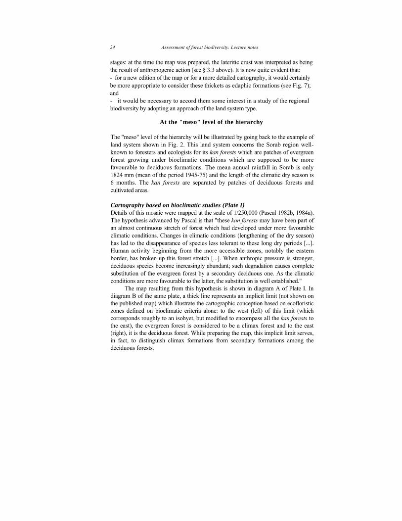
The "meso" level of the hierarchy will be illustrated by going back to the example of land system shown in Fig. 2. This land system concerns the Sorab region well-known to foresters and ecologists for its kan forests which are patches of evergreen forest growing under bioclimatic conditions which are supposed to be more favourable to deciduous formations. The mean annual rainfall in Sorab is only 1824 mm (mean of the period 1945-75) and the length of the climatic dry season is 6 months. The kan forests are separated by patches of deciduous forests and cultivated areas.
Cartography based on bioclimatic studies (Plate I) Details of this mosaic were mapped at the scale of 1/250,000 (Pascal 1982b, 1984a). The hypothesis advanced by Pascal is that "these kan forests may have been part of an almost continuous stretch of forest which had developed under more favourable climatic conditions. Changes in climatic conditions (lengthening of the dry season) has led to the disappearance of species less tolerant to these long dry periods [...]. Human activity beginning from the more accessible zones, notably the eastern border, has broken up this forest stretch [...]. When anthropic pressure is stronger, deciduous species become increasingly abundant; such degradation causes complete substitution of the evergreen forest by a secondary deciduous one. As the climatic conditions are more favourable to the latter, the substitution is well established."
The map resulting from this hypothesis is shown in diagram A of Plate I. In diagram B of the same plate, a thick line represents an implicit limit (not shown on the published map) which illustrate the cartographic conception based on ecofloristic zones defined on bioclimatic criteria alone: to the west (left) of this limit (which corresponds roughly to an isohyet, but modified to encompass all the kan forests to the east), the evergreen forest is considered to be a climax forest and to the east (right), it is the deciduous forest. While preparing the map, this implicit limit serves, in fact, to distinguish climax formations from secondary formations among the deciduous forests.

Landscape analysis and vegetation mapping 25
26 Assessment of forest biodiversity. Lecture notes

Landscape analysis and vegetation mapping 27

28 Assessment of forest biodiversity. Lecture notes
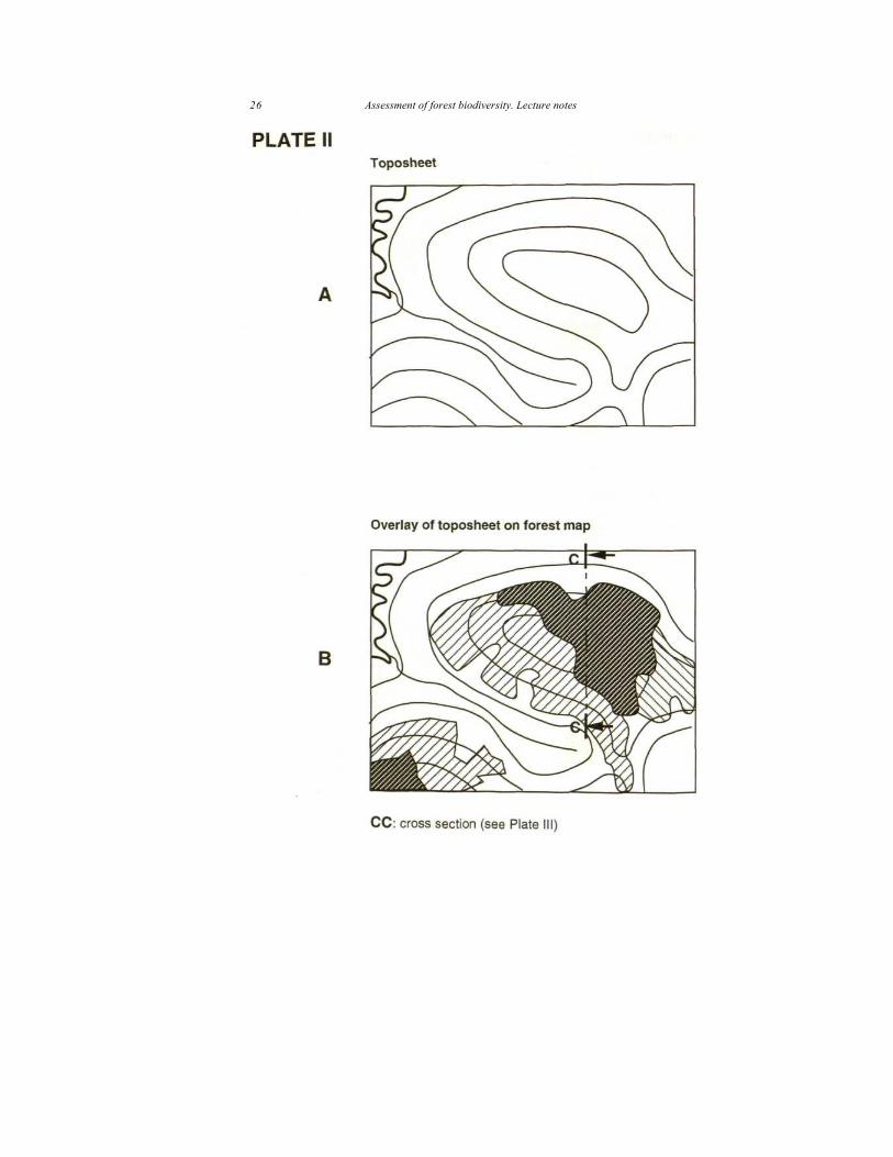
Observations on land system, land unit, and soils (Plates II and III) The land system is made up by very wide convex interfluves (2-3 km wide). A cross-section through a land unit, presently an interfluve (Plate II-A), allows to identify the different land facets.
A short, often indurated, slope follows the convex centre of the interfluve. The limit between the interfluves and beginning of the slope is marked by a strip of ferricrete outcrops, often dismantled in blocks by roots of trees. Lower down on the slope, a very thick laterite horizon is observed at a shallow depth which is sometimes exploited for the manufacture of bricks. This laterite has a vesicular facies.
The valleys are completely modified by human activity and often widened to the detriment of the non-indurated zones of the slopes. They are now used for cultivating rice and for water tanks.
The maximum difference in altitude between interfluves and valleys is not more than 50 m and the evergreen and semi-evergreen stands appear to be located on the interfluves.
Soils of the interfluves: the humiferous horizons, which are about 50 cm thick are dark reddish brown in colour and have very little ferruginous gravels near the surface, but much deeper down; they have a massive structure associated with a crumb structure and a sandy-clay-loam texture. The non-humiferous horizons are red, very gravelly with sandy-clay-loam texture and massive structure. The cation exchange capacity in the deep horizons (lacking significant organic matter) is quite low, between 9 and 11 meq/l00g when expressed in function of the total soil. When related to clay alone, it is around 16 meq/l00g. On the other hand, it is higher, almost double, in the organic horizons and the percentage of saturation is also higher, varying between 75 and 100 %.
Relationship between land system and distribution of the vegetation (Plate IV) The slopes, when not cultivated, are covered by deciduous formations. The kan forests are confined to the gravelly soils of convex interfluves. The existence and preferential location of the kans have been interpreted (Bourgeon & Pascal 1986) as the consequence of the high water holding capacity of these gravelly soils; in the absence of measurements made in India, it was interpreted as follows: - by first considering the important difference in depths exploitable by roots that exists between soils of the interfluves (depth > 2 or 3 m) and of the slopes (depth ± 0.5 m); - by analogy with similar cases often described in West Africa (Avenard 1971, Peltre 1977).

Landscape analysis and vegetation mapping 29

30 Assessment of forest biodiversity. Lecture notes
While interpreting the distribution of the vegetation for cartographic purposes, it becomes possible to substitute a strictly bioclimatic hypothesis by a pedoclimatic one. By drawing the limits of deep gravelly soils of interfluves on a physiognomic vegetation map (Plate IV), it becomes possible, among the deciduous forests, to distinguish those which are found on shallow soils with very little likelihood of once having been evergreen forests, from those which had the same edapho-climatic conditions as the kan forests and could therefore be interpreted as secondary deciduous forests. A sampling design aimed at estimating the regional biodiversity should take these subdivisions into account.
It should be noted that in this approach, the kan forests and deciduous forests should be considered as formations linked to particular pedoclimates. It would be improper to state that the kan forests are edaphic formations and the deciduous forests on the slopes are climax formations. It is the distribution of the vegetation for the entire land system which may be considered as dependent on the quality of soils, and hence edaphic, within a broad bioclimatic context.
To arrive at these conclusions, it is important to remember that it was necessary to consider the components of the land system, viz. land units and even land facets. Integrating an analysis of the land system type in inventory operations would involve not just drawing the external limit of each land system, but also explaining its internal structure. To illustrate this more precisely, two possible applications of the researches carried out in Sorab can be envisaged: - for a detailed study of the regional biodiversity, it would be enough to work on one, or few, representative land units in order to (i) locate the strip of ferricrete outcrops, (ii) carry out the exercises illustrated in Plate IV, and finally (iii) to study sample plots in each of the formations thus delineated; - if the existing vegetation maps are to be modified, a morphopedological sketch map should be prepared at a medium scale (1/50,000) to delineate the strip of ferricrete outcrops. This would require having access to aerial photographs (not available in India) or, for want of them, a good satellite image accompanied by toposheets at 1/50,000. Field work would be relatively easy to accomplish because it would only consist in locating ferricrete blocks and outcrops. The exercise illustrated in Plate IV should then be applied to the entire region of kan forests.

Landscape analysis and vegetation mapping 31
Other well-known cases Such an influence of soils on the vegetation, which is expressed by a
preferential localisation of forests in zones which are topographically high, is relatively rare. Most often the densest formations are observed in low land areas, especially if the presence of a shallow water table helps the vegetation to maintain itself during a long dry season (Fig. 6) or if a ferricrete occupying the interfluve hinders the growth of a dense vegetation (Fig. 7).
Figure 6. Example of land system where the pedo-climate is modified by the presence of a shallow water table.
Lateritic mesa
Figure 7. Example of land system where a ferricrete constitutes a major constraint for the forest.
How to introduce geomorphological analysis in phytogeographic inventory operations
Geomorphological analysis, to be most useful, should precede the setting up of sampling plots to describe forest stands. In the examples just cited, geomorphological analyses were not carried out by vegetation mapping experts. This will generally be the case as it is difficult to be a good forester or a good botanist and, at the same time, have a sufficiently extensive knowledge in geomorphology and soil sciences.
The integration of an analysis of the terrain classification type with a traditional vegetation mapping approach should pass through 3 stages.

32 Assessment of forest biodiversity. Lecture notes
Collection of basic data
Whether or not associated with the services of a geomorphologist, the phytogeographer should first gather the existing information on land forms and soils. He would have already procured, for his own work on vegetation mapping, aerial photographs, topographic maps, satellite imageries, as well as all the available botanical and forestry works. In addition to these, he should search for: - toposheets at a large scale, even if the map to be prepared is at a medium or small scale; - published geomorphological maps (there are several, especially for Vietnam); - geological maps, paying particular attention to those which provide information on superficial deposits; - pedological maps, searching for detailed documents even if they cover only a small part of the area to be mapped; - books, dissertations and research papers dealing with geology, physical geography and soils of the region under consideration.
Outline of a zoning of the zone to be surveyed
From this documentation he should try to: - draw up a hierarchic framework (like the one in Fig. 2) to illustrate his analysis in terms of terrain classification; - delimit, if possible, the different land systems and pay more attention to those where (i) the plant cover is still well conserved and (ii) the organization of the landscape seems to influence the characteristics of the vegetation, for which a study of aerial photographs would be extremely useful.
Reasoned field work according to the land systems
A sketch of the different land systems in the zone to be surveyed (in the form of cross sections, block diagrams and detailed maps) will enable the drawing up of a carefully reasoned sampling plan which will help in establishing floristic lists.

Landscape analysis and vegetation mapping 33
References
Avenard J.M. 1971. La répartition des formations végétales en relation avec l'eau du sol dans la région de Man-Touba. Trav. et Doc. ORSTOM, 12, 159 p.
Bates R. L., Jackson J.A. (Eds.). 1989. Glossary of Geology. 3rd édition. American Geological Institute, Alexandria, Virginia. 788 p.
Bourgeon G. 1989. Reconnaissance soil map of forest area, 1/1 000 000 scale, sheet WESTERN KARNATAKA AND GOA. Travaux de la section scientifique et technique, Institut Français de Pondichéry, hors série 20, explanatory booklet 96p + annexes 108p.
Bourgeon G., Pascal J.-P. 1986. Influences des héritages morpho-pédologiques dans la répartition des formations forestières : région de Sorab-Siddapur (Inde du sud). Bois et Forêts des Tropiques, 214: 3-21.
Brabant P. 1992. Pédologie et système d'information géographique. Comment introduire les cartes de sols et les autres données sur les sols dans les SIG. Cah. ORSTOM, sér. Pédol., 27(2), 315-345.
Christian C.S., Stewart G.A. 1953. General Report on Survey of Katherine-Darwin Region, 1946, C.S.I.R.O. Aust. Land Res. Ser., N° 1.
F.A.O. 1989. Classification and mapping of vegetation types in Tropical Asia. FAO, Rome, 170 p.
Ferry B. 1994. Les humus forestiers des Ghâts occidentaux en Inde du Sud. Facteurs climatiques, édaphiques et biologiques intervenant dans le stockage de la matière organique du sol. Publications du département d'écologie, Institut Français de Pondichéry, 34: 260 p.
Legris P. 1963. La végétation de l'Inde : écologie et flore. Travaux de la section scientifique et technique, Institut Français de Pondichéry, 6.
Ollier C.D. 1977. Terrrain classification: methods, applications and principles. In: John R. Hails Ed, Applied Geomorphology, pp. 277-316, Elsevier, Amsterdam..
Pascal J.-P. (With the collaboration of S. Shyam-Sunder, V.M. Meher-Homji). 1982a. Forest Map of South India, 1/250 000 scale, sheet Mercara-Mysore. Travaux de la section scientifique et technique, Institut Français de Pondichéry, hors série 18a.
Pascal J.-P. (With the collaboration of S. Shyam-Sunder, V.M. Meher-Homji). 1982b. Forest Map of South India, 1/250 000 scale, sheet Shimoga. Travaux de la section scientifique et technique, Institut Français de Pondichéry, hors série 18b.
Pascal J.-P. (With the collaboration of S. Shyam-Sunder, V.M. Meher-Homji). 1984a. Forest map of South India, 1/250 000 scale, sheet Belgaum-Dharwar- Panaji, Travaux de la section scientifique et technique, Institut Français de Pondichéry, hors série 18c.

34 Assessment of forest biodiversity. Lecture notes
Pascal J.-P. 1984b. Les Forêts denses humides sempervirentes des Ghâts Occidentaux de l'Inde. Travaux de la section scientifique et technique, Institut Français de Pondichéry, 20 : 364 p.
Pascal J.-P. 1986. Explanatory booklet on the Forest Map of South India. - Travaux de la section scientifique et technique, Institut Français de Pondichéry, hors série 18.
Peltre P. 1977. Le "V" Baoulé (Côte-d'Ivoire centrale). Héritage géomorphologique et paléoclimatique dans le tracé du contact forêt-savane. Trav. et Doc. ORSTOM, 80, 198 p.
Peterschmitt E. 1993. Les couvertures ferrallitiques des Ghâts occidentaux en Inde du Sud. Caractères généraux sur l'escarpement et dégradation par hydromorphie sur le revers. Publications du département d'écologie, Institut Français de Pondichéry, 32: 145 p + annexes.
Summerfield M.A. 1991. Global Geomorphology. Longman, Singapore, 537 p. Swamy H.R., J. Proctor 1994. Rain forests and their soils in the Sringeri area of
the Indian Western Ghats. Global Ecology and Biogeography Letters, 4, 140- 154.
Thomas M.F. 1994. Geomorphology in the Tropics: a study of weathering and denudation in low latitudes. John Wiley & Sons, Chichester, 460 p.
Tricart J. 1965. Principes et méthodes de la géomorphologie. Masson, Paris, 496 p.

Interpretation of satellite images for vegetation mapping
B.R. Ramesh
Introduction
Rapid depletion of biodiversity is of major concern the world over, more so with respect to the tropics which house between 2.5 and 15 million of the reported species (Parker 1982, Arnett 1985, Erwin 1983, Wilson 1988). Much of the biodiversity is confined to tropical forests.
Remote sensing could play a major role in detecting the diversity of habitats and vegetation over large areas, in addition to monitoring the spatial and temporal changes in them.
Remote sensing provides information about objects on the earth's surface without physically coming into contact with them. The satellite's sensors detect the reflected energy from objects and convert them into photographic images. The characteristics of an object can be deduced from the spectral variations in its reflected energy.
Spectral reflectance of the vegetation is quite distinctive (Fig. 1). Strong absorption of chlorophyll radiation occurs in the blue (0.48 µm) and red (0.68 µm) bands of the visible range. The reflectance in the green region of the light spectrum, on the other hand, is evident between 0.52-0 and 60 µm. Strong reflectance occurs at near the infrared region (0.75-1.3 (µm). The reflectance ratio between the visible and near infrared bands are sensitive indicators of the growth and vigour of the vegetation. Thus, plant communities with distinct seasonal peaks of growth and phenological activity can markedly affect the spectral reflectance. Other small scale changes in the vegetation of an area like a canopy gap following the death of an individual tree, or major changes, for example, due to anthropogenic pressure (including fire and flood), can also be detected using remote sensing.

36 Assessment of forest biological diversity. Lecture notes
Figure 1. Vegetation reflectance spectrum (from Current Science 1991)
A good example is the dry deciduous forest where trees shed their leaves during the dry period and show differential spectral reflectance as compared to the evergreen forest. In a satellite image, these two formations appear very distinct. Further, the density and combination of different colours can be used to interpret the degradations.
Worked example
False Colour Composite (FCC) picture with band 2, 3, 4 of either LANDSAT or IRS taken during the dry period (January to March) is ideal to demarcate the different physiognomic conditions of South India.
Dense evergreen forests appear bright red. Certain plantations (coffee, rubber and eucalyptus) also give similar colour. This has to be verified on toposheets and by fieldwork.
Semi-evergreen and disturbed evergreen forests show lesser density of red colour and appear to be less homogeneous in texture visually. A mixture of pink indicates thickets in their serial stages.
Deciduous forests appear homogeneously brown to greyish or reddish brown during leafless period in dense formations. Disturbed forests and degradation stages from woodland to savanna woodland, and tree savanna to shrub savanna show a gradual shift from mottle brown to grey. As deciduous forests are fire prone, the burnt area appears black or dark grey. Scrub woodland, grasslands and thickets are open formations with clumps of shrubs and scattered trees, with both evergreen and deciduous elements. This kind of physiognomy appears grey or pinkish grey.
Plantations of different species are depicted differentially with respect to age, location and species. For example: teak and certain softwood plantations appear light

Assessing species richness and diversity 37
grey during the deciduous season. They can only be recognised if they are surrounded by dense evergreen forests, but not if they are located within deciduous forests. Tea plantations appear pink in colour. Rubber and coffee appear red. Cardamom cannot be distinguished because they are grown under a canopy cover.
Limitations
- Remote sensing cannot give information about floristics; - Needs ground truthing for initial interpretation and a posteriori checking; - The colours attributed to the above physiognomic formations have been found to vary, depending on the way in which the images are processed; - Unlike with aerial photographs, satellite pictures do not allow precise density classifications of the canopy. The advent of high resolution satellite images (IRS 1C and others) with pixells less than 10 m x 10 m in parchromatic are modifying this situation. - Image resolution and band selection are important for accurate interpretation of the vegetation.
Suggested reading Parker S.P. 1982. (Ed.) Synopsis and classification of living organisms. McGraw-
Hill, New York. Arnett R.H. 1985. American Insects: A Handbook of the Insects of America North
of Mexico. Van Nostrand Reinhold, New York. Erwin T.L. 1983. Beetles and other insects of tropical forest canopies at Manaus,
Brazil, sampled by insecticidal fogging. In Tropical Rain Forest: Ecology and Management (Ed.) Sutton, S. L., Whitmore, T. C. and Chadwick, A. C. Edinburgh, pp. 59-75. Blackwell Scientific Publications, London.
Wilson E.O. 1988. The current state of biological diversity. In Biodiversity (Etd.) E.O. Wilson & F.M. Peter, pp. 3-18, National Academy Press, Washington.
Current Science 1991. Special issue on Remote Sensing for National Development, 61.
Hobbs R.J., Mooney H.A. (Ed.). 1990. Remote sensing of Biosphere functioning. Springier-Verlag, New York.
Pascal J.-P. 1986. Explanatory booklet on the Forest Map of South India. - Travaux de la section scientifique et technique, Institut Français de Pondichéry, hors série 18.

38 Assessment of forest biological diversity. Lecture notes
Assessing species richness and diversity at the community level: methodological background
François Houllier, Clémentine Gimaret-Carpentier
Abstract
Most difficulties in biodiversity assessment arise from the very fact that it is essentially a matter of measuring a variability and not an average: counting the number of species which are different from each other rather than the average number of stems per ha. As a consequence: the usual sampling strategies which aim at estimating an average and its precision are not necessarily adapted; much more than for other resources, assessing biodiversity is scale- and level-dependent.
Another important methodological point for regional studies and across-ecosystems studies is that the assessment of species diversity and richness of ecosystems is the dual viewpoint of the study of the ecological niche and geographic distribution of species.
In this context, this lecture reviews the following topics: - General statistical background: sampling design and estimators; accuracy and precision; random, systematic, stratified and cluster sampling. - Assessment of species richness:
• number of observed species and species list; • why the natural estimator obtained as the number of observed species is biased
(it always underestimates the true richness); • the cumulative species-area and species-individual curves and the correction
method designed by Sanders and Hurlbert to compare samples of different size;
• the relative efficiency of various sampling designs and estimators: random, systematic and stratified sampling, fixed-area vs. fixed-number of individuals plots, non parametric estimators.
- Assessment of species diversity: • diversity as a combination of species richness and evenness and the role of
rare species;

Assessing species richness and diversity 39
statistical properties of the usual estimators of Simpson's and Shannon's indexes of diversity: accuracy and precision.
Introduction
Most methodological difficulties in biodiversity assessment arise from the very fact that it is essentially a matter of measuring a variability rather than estimating an average: counting the number of species which are different from each other rather than enumerating the total number of stems per ha or estimating their mean diameter.
That diversity should actually be considered as some form of variance (Pielou 1995) has two important methodological consequences: (i) the usual sampling strategies which aim at estimating means and their precision (i.e., the standard error) are not necessarily adapted (Box 1); (ii) assessing biodiversity, much more than other resources, is scale-dependent and level-dependent (Box 2).
Box 1. Sampling for richness: a comparison with stratified random sampling. Let us take the case of a forest made of different compartments (or stands, or ecosystems), where one of these compartments contains several unique species (here VI is the only stand that contains species e, f and g), while other compartments contain only a few, but common, species. If we want to estimate average volume per ha, this stand should be sampled as intensively as the others. But if we are interested in species richness then we should survey this stand more intensively than others: else we might miss the rare species (e, f and g). We can somehow compare this situation to the case where stratified sampling is applied to estimate the volume per ha and the internal variance of one stand is high: in such a case we indeed know that the optimum allocation of samples requires that more samples are laid in the highly variable stand than in the others (Cochran 1977, Scherrer 1983).
Scale refers to spatial units: the size of the spatial unit for which estimates are to be made as well as the size of the elementary sample units. Level refers to the taxonomic hierarchy: e.g., genotype, species, genus, family, etc. The fact that these two types of hierarchy, spatial and taxonomic, are intertwined with the hierarchical approach used to name ecological entities (from the biosphere to spatially distinct populations, through landscapes, ecosystems and communities) adds to the

40 Assessment of forest biological diversity. Lecture notes
conceptual and technical difficulty involved when dealing with biodiversity. In this lecture, we mainly consider the species richness and diversity within ecosystems and communities which may be more or less large, i.e., within a range of, say, 1 to 1 000 ha.
Box 2. Scale-dependence of species richness. The scale-dependence of diversity and richness measures can be easily understood from the usual species cumulative curve: when the study area increases, the species richness also increases, but in a non-linear way. In this virtual example, species are denoted with letters (a, b, etc.) and are spread over an ecosystem made of 4 compartments. 4 such ecosystems are figured and 4 methods are utilized to assess their richness: (i) average species richness per compartment; (ii) average species per group of 2 compartments; (iii) total species richness in the ecosystem. They show that richness ranking varies according to the scale at which it is estimated. There is no canonical way to standardise richness (no such standard unit as m3.ha- 1 for volume): to compare species richness among two different ecosystems, we may count their total number of species (but it is likely to "favour" the largest ecosystem), or we may estimate the average number of species in standardised sample plots (e.g. usual forest inventory fixed-area plots) or in one ha. But, all these measures may yield different results. The same happens when diversity is hierarchically decomposed along taxonomic groups: family, genus, species, genotypes.
Another important methodological point for regional studies of species diversity is that there are two reciprocal viewpoints: (i) a species-by-species approach where the emphasis is put on the ecological niche and geographic distribution of species across ecosystems; (ii) an ecosystem-oriented approach where the focus is on the richness and diversity within different ecosystems or types of ecosystems. This duality is best shown when the correspondence analysis technique is applied to phytosociological data (Box 3).
Assessing species richness and diversity 41
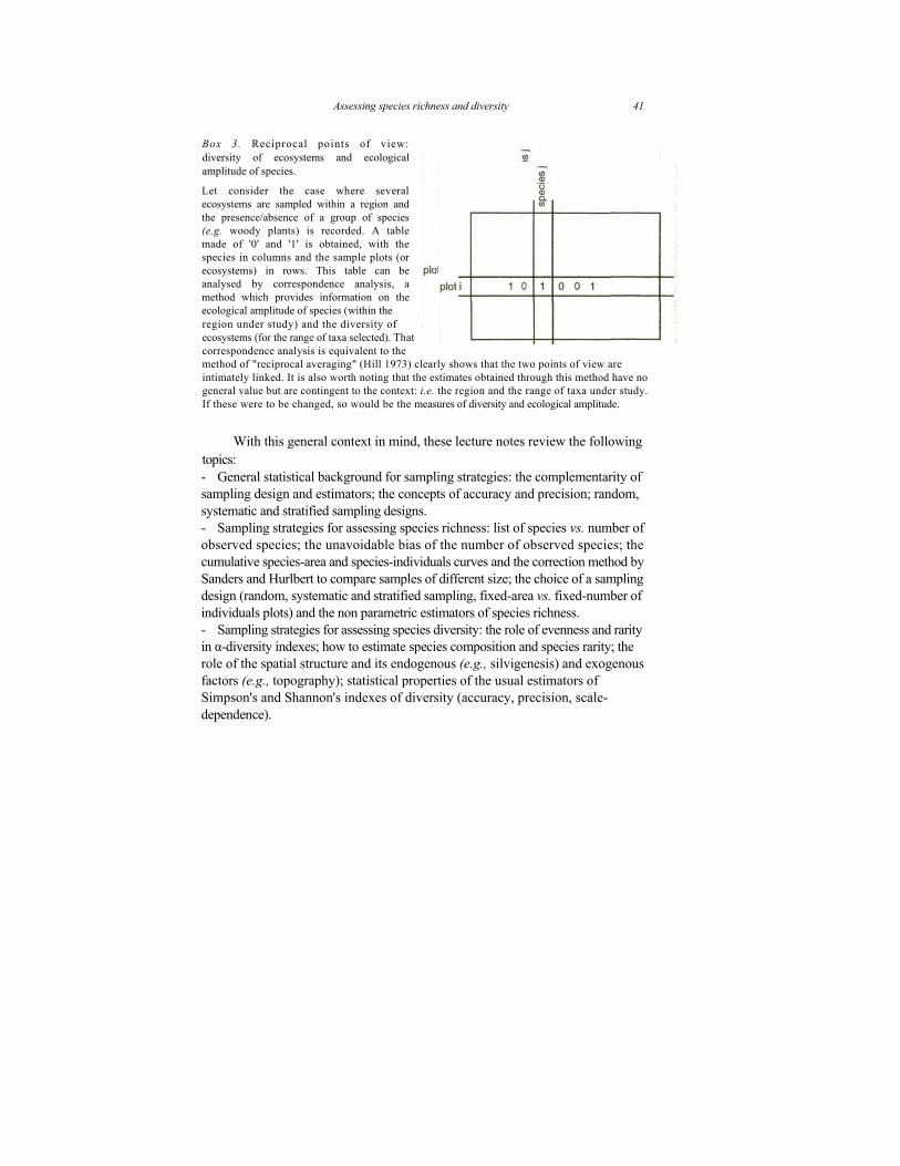
Box 3. Reciprocal points of view: diversity of ecosystems and ecological amplitude of species. Let consider the case where several ecosystems are sampled within a region and the presence/absence of a group of species (e.g. woody plants) is recorded. A table made of '0' and '1' is obtained, with the species in columns and the sample plots (or ecosystems) in rows. This table can be analysed by correspondence analysis, a method which provides information on the ecological amplitude of species (within the region under study) and the diversity of ecosystems (for the range of taxa selected). That correspondence analysis is equivalent to the method of "reciprocal averaging" (Hill 1973) clearly shows that the two points of view are intimately linked. It is also worth noting that the estimates obtained through this method have no general value but are contingent to the context: i.e. the region and the range of taxa under study. If these were to be changed, so would be the measures of diversity and ecological amplitude.
With this general context in mind, these lecture notes review the following topics: - General statistical background for sampling strategies: the complementarity of sampling design and estimators; the concepts of accuracy and precision; random, systematic and stratified sampling designs. - Sampling strategies for assessing species richness: list of species vs. number of observed species; the unavoidable bias of the number of observed species; the cumulative species-area and species-individuals curves and the correction method by Sanders and Hurlbert to compare samples of different size; the choice of a sampling design (random, systematic and stratified sampling, fixed-area vs. fixed-number of individuals plots) and the non parametric estimators of species richness. - Sampling strategies for assessing species diversity: the role of evenness and rarity in α-diversity indexes; how to estimate species composition and species rarity; the role of the spatial structure and its endogenous (e.g., silvigenesis) and exogenous factors (e.g., topography); statistical properties of the usual estimators of Simpson's and Shannon's indexes of diversity (accuracy, precision, scale- dependence).

42 Assessment of forest biological diversity. Lecture notes
Sampling strategies: generalities
Objectives of forest inventories
As a first point it is important to emphasise that stating the objectives of a survey is always the most crucial point. For example: - Is it aimed at estimating standing volume or biomass, or is it aimed at assessing the species richness and diversity? - Is it aimed at mapping the physiognomy of the vegetation (forest cover being the most important criterion) or the ecological nature of the ecosystems (i.e., ecofloristic type)? - At which level should the result be reasonably accurate and precise: world, country, state or region, administrative forest unit, ecosystem?
A second major factor is obviously the cost of the survey. It is often thought that transforming a timber-aimed inventory into a plant-diversity-oriented survey is a good way to make economies. This is partly true (it is not necessary to go twice to the field) but such a transformation also needs additional resources in terms of money and time (spent in each plot) as well as of human skills (e.g., appointment of botanists and/or training of survey crews) and of data analysis (e.g., new computer routines to be developped).
An historical analysis of the evolution of forest inventories in Western countries would probably show that their focus successively shifted from assessing standing stock (forest area, volume and increment) towards estimating the future wood available cut, monitoring changes (in forest area, in standing volume and in volume increment), assessing total biomass (and not only the volume of timber) and, later on, carbon contents, forest health, non timber forest products and ecological diversity. On the one hand, these trends are natural consequences of the technical evolution: as such, they account for the progressive accumulation of data and knowledge (monitoring is obviously subsequent to a first assessment); on the other hand, they are the results of the changes in national or international forestry issues and concerns (deforestation, loss of biodiversity, global warming, etc.). Nevertheless, it remains that the design and organisation of most national forest inventories in the world are still mainly timber-oriented, not biodiversity-oriented.
Sampling strategy, accuracy and precision
A sampling strategy has always two components, which are closely associated: (i) a sampling design, that is the way samples are drawn from the population or domain under study; (ii) estimators, that is equations and formulas that are used to get estimates (of the unknown values which constitute the goal of the surveyor) from

Assessing species richness and diversity 43
the samples. The articulation of the sampling design and the estimators requires a statistical model: without such a model there is no possibility to infer estimates from the observations. It happens that this articulation is not strict: for example, it is possible (but not necessarily optimal, nor wise) to use a systematic sampling design and apply the estimators derived from the theory of simple random sampling.
There are several criteria to assess the quality and reliability of the estimates derived from a sampling strategy. It is indeed worth reminding that no survey, but an improbable exhaustive and perfect inventory of a small finite population, will ever provide the exact value which the survey is aimed to assess. Two statistical concepts are of prime importance for samplers: the accuracy and the precision of the estimates.
Let us define µ. the unknown value (for example, µ is the mean value of volume per ha), which is estimated by µ (for example, µ = y the average value of volume per ha observed in different sample plots). The accuracy of µ refers to its unbiasedness: if we repeat the survey several times (with the same sampling design), µ should exhibit no systematic —neither positive nor negative— departure from µ: if E[ µ ],= µ, µ is unbiased; B[ µ ] = E[ µ ] - µ is the bias of µ .
But even for an accurate (that is unbiased) estimator, there is always a random variability of µ around its theoretical expected value E[ µ ]. The precision of µ is the measure of this variability: it is usually defined thank to the estimation variance (or sampling variance), V[ µ ], and its square root, the standard error of the estimator, which describe the dispersion of the estimator around its expected value.
Precision and accuracy are often combined in the mean square error, MSE[ µ ], and its root, RMSE[ µ ], which describe the dispersion of the estimator around the true but unknown value:
The standard error of the estimator can also be used to build confidence-intervals which give an estimated range where the true unknown value is likely to be.
Some classical sampling strategies
Let us note y the variable whose mean value, µ, we want to estimate. Let also σ2
be the variance of y. Most common estimators of µ are in fact linear estimators (i.e., linear combinations of the observed data) and are designed so as to be the best

44 Assessment of forest biological diversity. Lecture notes
linear unbiased estimators (under a given statistical model). Their statistical properties are well known for most standard sampling designs, which aim at assessing usual mean characteristics such as mean volume, number of stems or basal area per ha. But we will see below that this is not the case for the estimates of species richness and diversity: their estimators are not always linear, some are biased and some have an unknown variance.
Here we only review four classical and basic strategies presented in most sampling or forest inventory textbooks (e.g., see Lanly 1981); regression sampling and sampling at successive occasions (i.e., monitoring) are not considered (for the latter, one may refer to the lecture note on permanent plots). These basic strategies mainly differ according to: (i) the respective weight given to precision and to cost efficiency; (ii) the availability or absence of external prior information that helps making the sampling more efficient. With respect to the latter point, simple random sampling, the most famous strategy, could be termed "you don't know much, you don't get much". Actually, operational as well as research forest surveys usually combine several of these basic strategies.
Table 1. Standard sampling strategies for estimating the mean, µ, of a variable, y: estimators and their variance (from Scherrer 1983 and Cochran 1977).
Note: All these estimators of µ are unbiased under the respective assumptions of each sampling strategy. Estimators of V[ µ ] are obtained by replacing the theoretical variances by their usual
the theorical estimates (for example: 2σ =s2= )1)( 2
1 −−∑
= nyyi
n
i
Estimation variances given here do not include the correction factor due to sampling intensity. If sampling intensity is high, this factor must be included and will diminish the estimation variance.

Assessing species richness and diversity 45
Simple random sampling This classical reference sampling strategy consists in drawing n independent samples, yi (l≤i ≤n), with a uniform probability. The formulas are simple and well known (see Table 1), but it is often forgotten that laying a true random sample in the field is not so easy and actually requires a lot of rigour. Because of their simplicity the formula associated to simple random sampling are often utilised, although they are sometimes not appropriate.
Stratified random sampling Most national forest surveys which are based on a two-stage process —(i) mapping from either aerial photographs or satellite imagery, (ii) field measurements in sample plots— use stratification for the second stage of the survey. The rationale for this strategy is to split the domain under study, which has an area S, into H subdomains or strata, h(1≤h≤H), which are more homogeneous than the whole domain itself and have an area Sh (1≤h≤H). Each strata is then sampled with nh observations, yi,h
(1≤h≤H, 1≤i≤nh). The overall variability is thus divided into two components, the between-strata
variability, which is exhaustively sampled, and the within-strata variability, σh2
(1≤h≤H), which remains uncontrolled. Stratification can only be achieved by using some prior external information such as aerial photographs. The efficiency of stratified random sampling chiefly depends on the relative magnitude of the between-and within-strata variability, that is on the capability of the stratification criteria to account for the global variability of y.
Another reason for using stratification is when results are simultaneously sought for the total domain and for some of its components (e.g. different forest types).
Systematic sampling Several empirical studies followed by more theoretical developments have shown that systematic sampling is usually a very efficient strategy when no prior information is available (so that stratified sampling cannot be applied). The reason is that systematic sampling ensures a good and homogenous coverage of the domain to be sampled. There is one exception to this general rule: when the phenomenon under study exhibits a periodic behaviour.
Systematic sampling consists in choosing a grid with steps on x and y, and a randomly selected starting point. The difficulty with this strategy is that the best linear unbiased estimators are not as simple as for other designs. The choice of unbiased and efficient estimators requires that a spatial statistical model of the population be formulated (Journel & Huijbregts 1978). Such spatial models are out
46 Assessment of forest biological diversity. Lecture notes
of the scope of this lecture. However, an interesting output of the study of systematic sampling is that it shows that estimators and their variance depend on: - the spatial structure of population under study, e.g., the spatial correlation between two point according to their mutual distance, - the number, size and spatial arrangement of the samples, - the size of the domain to be estimated and its position vis-à-vis the samples.
For example, if the phenomenon exhibits some regularity (i.e., the value of y at x is positively "correlated" to its value at a short distance from x), the mean of sample observations is usually an unbiased estimator, but it is not the most efficient and its estimation variance is very different from —and, in fact, much lower than— the approximate estimation variance derived from the simple random sampling theory.
Cluster sampling Cluster sampling is an example of multilevel (or multidegree) sampling. Cluster sampling is a particular case of a two-level (degree) sampling design. It consists: (i) in partitioning the domain in N primary units among which n are randomly and independently selected; (ii) in further partitioning the primary units in M secondary units among which m are sampled in the n primary units already selected.
Let i denote the primary units and j denote the secondary units: observations are yij (1≤i≤n, l≤j≤m); the average estimated value for the primary unit i is noted y I; the variance among primary units is noted σh
2; the average variance within primary units and among secondary units is noted σw
2. Estimators are given in Table 1.
This sampling strategy is not very efficient in terms of precision, but can turn out to be a very good compromise when cost and travelling from sample to sample come into the picture. It has been popularised in forestry by the Swedish and Finnish national forest inventories which use cluster of secondary units organised in L-shaped or square "tracts".
Assessment of species richness
One of the most evident and, apparently, simple parameter to characterise ecological diversity is the species richness. As will be seen below, this parameter is however less simple than usually expected. Species richness depends only on the presence (vs. absence) of the species. It is thus based on binary data (Pielou 1995): it corresponds to the classical phytosociological approach and avoids to measure the abundance or frequency of the species. Other components of diversity include the frequency of the species and the evenness of their relative distribution. They will be dealt with in the next section.

Assessing species richness and diversity 47
How to characterise species richness
Species richness can be assessed by two ways: (i) by counting the number of species; (ii) by enumerating the list of species. In both cases, it must be clear that any survey, but an exhaustive inventory of a finite population, can only yield a biased estimate of species richness: the observed list or number of species always underestimate (or at best exactly equals) the actual species richness.
This very fact has been known for long and has generated many studies on the so-called collector's curves (Pielou 1995) also named the cumulative species-area and species-individual curves: these curves picture the cumulative number of distinct species observed when either the sampled area or the number of sampled individuals increases. These curves are monotonously increasing and usually have a logarithmic shape.
If we are interested in assessing the species richness of an ecosystem, region or country, nothing can replace the list of species: the number of species is only a by-product of this enumerative list and is of no use if the aim is to define a conservation strategy or to initiate monitoring. This fact is a very consequence of the qualitative nature of biodiversity. The major difficulty lies with rare species: there is no means by which we may be sure to observe them in a sample.
However, the number of species, whichever way it is estimated, can be useful in scientific studies which aim at assessing the effects of ecological factors on biodiversity (e.g., Box 4), the role of biodiversity in the functioning of ecosystems (Tilman & Downing 1994; Tilman et al. 1996) or the temporal changes in biodiversity. Note that, even in these cases, understanding the phenomena will often require a species-by-species analysis (e.g., which species did disappear? what are their ecological behaviour and requirements?).
As already mentioned in the introduction, one of the difficulty in assessing species richness (and diversity) stems from the fact that this variable is scale- and level-dependent. This can be further discussed, looking at the additivity of richness: - when richness is hierarchically broken according to taxonomic levels, the total richness at a lower level (e.g., species) is equal to the sum of richness within the broader classes (e.g., genus); - the same does not hold true when the spatial decomposition of richness is considered. If two communities are merged their total richness is not equal to the sum of their own richness (the number of species common to both communities must be substracted; e.g., see Box 2).
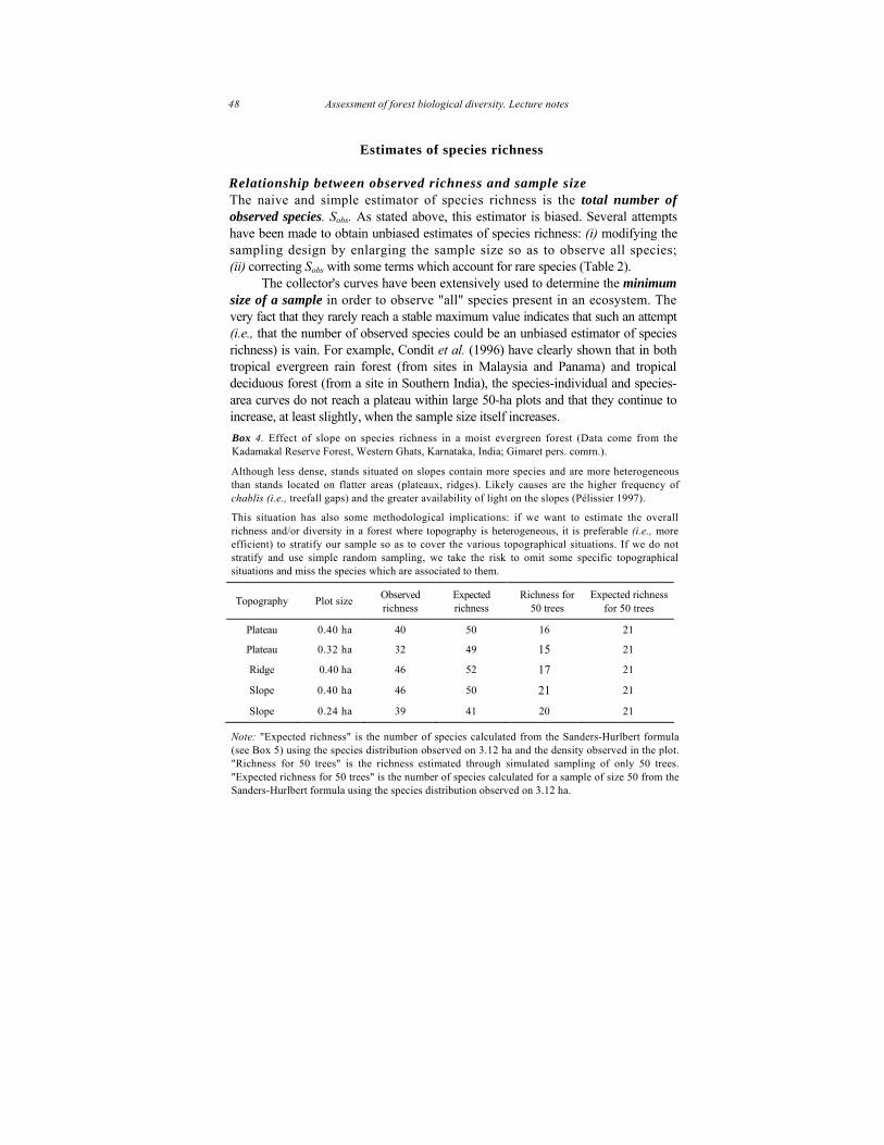
48 Assessment of forest biological diversity. Lecture notes
Estimates of species richness
Relationship between observed richness and sample size The naive and simple estimator of species richness is the total number of observed species. Sobs. As stated above, this estimator is biased. Several attempts have been made to obtain unbiased estimates of species richness: (i) modifying the sampling design by enlarging the sample size so as to observe all species; (ii) correcting Sobs with some terms which account for rare species (Table 2).
The collector's curves have been extensively used to determine the minimum size of a sample in order to observe "all" species present in an ecosystem. The very fact that they rarely reach a stable maximum value indicates that such an attempt (i.e., that the number of observed species could be an unbiased estimator of species richness) is vain. For example, Condit et al. (1996) have clearly shown that in both tropical evergreen rain forest (from sites in Malaysia and Panama) and tropical deciduous forest (from a site in Southern India), the species-individual and species-area curves do not reach a plateau within large 50-ha plots and that they continue to increase, at least slightly, when the sample size itself increases. Box 4. Effect of slope on species richness in a moist evergreen forest (Data come from the Kadamakal Reserve Forest, Western Ghats, Karnataka, India; Gimaret pers. comrn.). Although less dense, stands situated on slopes contain more species and are more heterogeneous than stands located on flatter areas (plateaux, ridges). Likely causes are the higher frequency of chablis (i.e., treefall gaps) and the greater availability of light on the slopes (Pélissier 1997). This situation has also some methodological implications: if we want to estimate the overall richness and/or diversity in a forest where topography is heterogeneous, it is preferable (i.e., more efficient) to stratify our sample so as to cover the various topographical situations. If we do not stratify and use simple random sampling, we take the risk to omit some specific topographical situations and miss the species which are associated to them.
Topography Plot size Observed richness
Expected richness
Richness for 50 trees
Expected richness for 50 trees
Plateau 0.40 ha 40 50 16 21 Plateau 0.32 ha 32 49 15 21 Ridge 0.40 ha 46 52 17 21 Slope 0.40 ha 46 50 21 21 Slope 0.24 ha 39 41 20 21
Note: "Expected richness" is the number of species calculated from the Sanders-Hurlbert formula (see Box 5) using the species distribution observed on 3.12 ha and the density observed in the plot. "Richness for 50 trees" is the richness estimated through simulated sampling of only 50 trees. "Expected richness for 50 trees" is the number of species calculated for a sample of size 50 from the Sanders-Hurlbert formula using the species distribution observed on 3.12 ha.

Assessing species richness and diversity 49
Box 5. Comparison of species richness among different ecosystems using samples of different size. • Using the collector's curve. Let consider the case where an average collector's curve has been established for a given type of ecosystems (e.g., low elevation moist evergreen forests in the Western Ghats of India) and suppose that this curve can be fitted with an analytical model: E[Sobs(n)] = f(n, θ), where θ are parameters and n is sample size (n could be replaced by A, the sample area). For example: f(n, θ) = 1 +θ.1n(n). Let now consider samples drawn from ecosystems or communities belonging to the type for which the collector's curve has been established: let ni, be their size and Sobs( their observed richness. The index Sobsi/E[Sobs(ni)] is independent of sample size and provides a means to rank samples according to their relative richness. In the virtual example below this ranking would be: sample 2<sample 3<sample 1.
Such a rule of thumb procedure has the advantage of being simple (provided the collector's curve exists and is reliable). Its main drawback is that this method is arbitrary and that there is no theoretical background for the definition of such an index. •Sander’s & Hurlbert's rarefaction method. This method aims at standardising estimates of species richness to the same minimum sample size. Let n be the total number of individuals recorded in a sample and ni be the number of individuals of the ith species. Let m (m<n) be the sample size to which species richness estimate should be scaled down. The probabilitv for a given species not to be in a m-size random and independent subsample is:
⎪⎩
⎪⎨⎧
=∉−≥−−
−−=⎟⎟
⎠
⎞⎜⎜⎝
⎛⎟⎟⎠
⎞⎜⎜⎝
⎛ −=∉−<
0)samplePr(, if !)!.()!)!.((
/
)samplePr(, if
i
i
iiii
spmnninmnnmnnn
mn
mnn
spmnn
The expected number of species in a m-size random and independent subsample is obtained by summing the probability of the species to be included:
E[Sobs(m)] = ∑= ⎥⎦
⎤⎢⎣
⎡−−
−−−
Sobs
ii
i
nmnnmnnn
1 !)!.()!)!.((1

50 Assessment of forest biological diversity. Lecture notes
The collector's curves can however be used in another way. If we consider an ecosystem which has been intensively sampled, it is possible to build several such curves by randomising the order of accumulation. This procedure provides an empirical way to estimate the variance and precision of Sobs for smaller samples.
In some studies, the focus is not on the absolute value of richness but on comparing the relative richness among different forest stands, ecosystems or communities. The collector's curves show that this goal can be reliably achieved only if the size of the sample is the same in the different stands. When sample size is not consistent across ecosystems to be compared, two strategies can be followed (Box 5): - If an average collector's curve has been established and is valid for the ecosystems to be compared, this curve can be used as a qualitative means for ranking different samples: however, the reliability of this method strongly depends on the reliability of the collector's curve itself and on its applicability to the ecosystems which are under comparison. - Sanders (1968) and Hurlbert (1971) have proposed the so-called "rarefaction method" to scale the estimate of species richness down to a common minimum sample size. This method is non parametric in the sense that it is only based on combinatorial analysis (under the assumption of random and independent sampling) and that it does not require the a priori existence of a collector's curve.
Non parametric estimators and rare species Another strategy to obtain more reliable estimates of species richness starts from the recognition that the problems stem from our inability to observe rare species. This strategy is based either on modelling the distribution of frequency of species (the frequency-rank diagram or the number of species-frequency diagram), or on correcting Sobs with additional terms which take the role of rare species into account. Several such estimators have been proposed (Table 2, Fig. 1). These estimators are named non parametric or distribution-free estimators because they make no statistical assumption, neither on the spatial distribution of the trees, nor on the shape of the frequency distribution of species.

Assessing species richness and diversity 51
Figure 1. Correction of the collector's curve using Chao l estimator. The observed number of species is increased by a term that takes rare species into account through a (the number of species represented by a single individual) and b (the number of species represented by exactly two individuals). Here: Sobs =4, a=2, b=1; the corrective term thus equals 2.
One of the method used to obtain such non parametric estimators consists in using the Jackknife procedure (Heltshe & Forrester 1983; Magurran 1988): - suppose there are n sample plots in which species are enumerated. The naive overall estimate of species richness is obtained by pooling these n plots: this estimate is noted Sobs; - Imagine that we remove the ith sample plot: we then get another estimate of species richness based on n-1 plots, which is noted S(-i); - From this estimate, we may derive a so-called pseudo-value of species richness defined as Si = n • Sobs - (n -1). S(-i); - The empirical mean of these n pseudo values yields an estimator of species richness (see the 1 st-order Jackknife in Table 2), whose variance can be estimated from the empirical variance of the pseudo values.
These non parametric estimators can be used to derive "corrected" species-area or species-individual curves where they replace Sobs. These "corrected" curves exhibit a very steep increase when sample size is small and then tend to stabilise quicker than the usual collector's curves, thus helping us in selecting a minimum sample size. However, recent studies (Condit et al. 1996) show that, in moist evergreen forests, even these "corrected" curves do not reach an upper stable value (a plateau), which would provide a simple estimate of the minimum sample size.

52 Assessment of forest biological diversity. Lecture notes
Table 2. Non parametric estimators of species richness (from Chao 1987, Colwell & Coddington 1994). Sobs= number of observed species; a= number of species represented by a single individual; b= number of species represented by two individuals exactly; L= number of species represented in one single plot; M= number of species represented in exactly two plots; n= number of plots; fj= number of plots that contain exactly j unique species.
Note: these four estimators contain the naive estimator of species richness to which a non-negative (except, may be, for the 2nd-order Jackknife) correction term is added. This additional term accounts for the proportion of very rare species (those which are observed only once in the samples) and rare species (those which are observed exactly once).
Another non parametric way to characterise and compare the pattern of species richness variations across several ecosystems is to perform a correspondence analysis on the presence/absence table of species in these ecosystems (Box 3). Correspondence analysis does not provide an absolute estimate of richness but provides a means to simultaneously compare the relative richness of sites (i.e., communities, ecosystems, stands) and the width of the ecological niche of the species that can be found in these sites. More recent data analysis techniques such as the canonical correspondence analysis (or the use of instrumental variables) help analysing the environmental factors which cause the changes in species richness (Ter Braak 1986, Gégout & Houllier 1996).

Assessing species richness and diversity 53
Which sampling design for species richness?
Here we focus on assessing species richness at the level of an ecosystem or a community (not of a landscape, a region or a country) in the context of a comparative approach across ecosystems.
An example of a design defined for South Indian moist evergreen forests is given in Fig. 2: this sampling design was used to get reference values for different types of ecosystems along a bioclimatic (low-elevation vs. high-elevation) and a disturbance (unlogged forests vs. logged forest and coffee plantations) gradient. Preliminary results are given in Table 3 for the influence of logging and altitude.
The choice of a sampling design cannot be made in general but some guidelines may be followed and adapted to every special case: - Because of financial and time constraints, it is generally preferable to sample plots or quadrats rather than scattered trees. Therefore, 2nd-degree sampling is often a good strategy (primary units being plots and secondary units being trees). - The main drawback with the above design is that the spatial distribution of species is rarely at random (e.g., pioneer species are clumped together in the openings and gaps). Therefore there should be several small plots (rather than a single large plot). The total size of the sample (i.e., number of sample trees or sample area) and its break up among plots can be decided only after considering some a priori available information: shape of the collector's curve, frequency of rare species, spatial pattern of the species, etc. - If we are only interested in species richness, plots with a fixed number of sample trees may be a better choice than plots with a fixed area. It is indeed preferable to think sample size in terms of individuals rather than of area. From observations in a South Indian moist evergreen forest (Gimaret et al. 1997) and other tropical forests (Condit et al. 1996), it turns out that the minimum total sample size should at least be of, say, 1 000 stems. - The procedures used to select the plots can be varied: the random and independent selection is probably the worse; systematic, transect or tract sampling (e.g., see Fig. 2) are better procedures which help "covering" the within-ecosystem natural variability; stratified sampling may also be a good choice if some ecological factors are known to influence the distribution of species (e.g., local topographical factors, see Box 4).

54 Assessment of forest biological diversity. Lecture notes
Figure 2. A sampling design for assessing tree species richness and α-diversity in moist evergreen dense forests of the Western Ghats (Gimaret pers. comm.). This design was defined for these forests (which have an actual richness of say 100-150 tree species in a 50-ha compartment) and was later adapted to coffee plantations (when the stands are not dense, the number of sample trees was reduced to less than 10 in size class). rl= distance to the 10th tree, r2= distance to the 10th sapling. Note: The total number of sample trees (i.e., 400) is below the minimum value derived from the collector's curve obtained with non parametric estimators: this choice was finally made after taking costs, time and other constraints into account. The two census thresholds help limiting the field work, while providing information on both smaller and larger trees. One of the drawback of this system is that it complicates the estimation of diversity because the latter also requires information on species frequency; richness per se does not require such information but the non parametric estimators use them.
One major difficulty is that it is fairly rare that we are only interested in species richness at one point of time: we also want to estimate species diversity, characterise stand structure, assess standing volume or biomass, understand the processes which determine the functioning of the stand, and set up a permanent system to monitor the changes! With these many other objectives in mind, it becomes rather difficult to rigorously define a sampling design and some compromises have to be made.

Assessing species richness and diversity 55
Table 3. Estimation of the tree species richness and diversity in moist evergreen forests along disturbance and altitudinal gradients in Coorg (preliminary results from Gimaret, obtained using the design described on Fig. 1). No clear trend comes out of these results which suggest that selective logging and altitude have only a mild impact on the total number of species. The figure is different if we consider the list of species: e.g., deciduous species are introduced as the result of human-driven forest degradation; the rate of endemic tree species decreases with altitude.
Site Forest type Altitude Sobs 1S λ
Uppangala Undisturbed evergreen ≈450 m 78 135 0,945 Uppangala Once-logged evergreen ≈350 m 68 92 0,960 Uppangala Disturbed semi-evergreen ≈200 m 67 102 0,955 Uppangala Secondary moist deciduous ≈200 m 80 121 0,948 Makut [67] Disturbed semi-evergreen 150 m 68 95 0,961 Makut [59] Undisturbed evergreen 450 m 76 99 0,946 Makut [52] Undisturbed evergreen 800 m 67 112 0,947
Kabbe Motte Undisturbed evergreen 1300 m 64 90 0,945
Note: the sampling design is described in Figure 1: 1S is the Chao 1 estimator defined in Table 2;
λ is the estimate of the Simpson's diversity index (see below); saplings and bigger trees are pooled together, irrespective of their relative frequency. Note that the two estimators of richness are fairly different.
Assessment of species diversity
Diversity: a combination of richness and evenness
Diversity combines two aspects: the species richness and the evenness (or equitability or dominance) of species distribution in the community. There are many different ways to assess diversity. They can be classified into two broad classes: - analysis of the distribution of species frequency, which can be compared to some theoretical models; - global diversity indexes which give more or less weight to evenness and richness. Some of these indexes may be derived from the analysis of species abundance (e.g., see the Fisher index below).

56 Assessment of forest biological diversity. Lecture notes
Models of species abundance
There are different ways to investigate the distribution of species abundance (or frequency). A first method consists in ranking the species according to their frequency, from the most abundant to the rarest: this yields the rank / abundance plot. A second method is based on counting the species according to their frequencies, which yields the classical frequency distribution plot.
For the distribution of species two classical models are often considered (Magurran 1988): - logarithmic series, where the number of species with j sample individuals is proportional to the jth term of the Taylor series of the logarithm: a = xj/j, where x and a are parameters to be estimated, a is the so-called Fisher's index of diversity, which can be directly estimated from the following implicit equation (Condit et al. 1996): Sobs = α ln(l + n/α ), where n is the size of the sample; - the lognormal distribution, where the number of species having an abundance of n sample individuals is proportional to a lognormal probability distribution function.
Two other models have been designed to represent the rank-abundance relationship (Magurran 1988)2: - geometric series, where the frequency of the species with rank i+l is systematically proportional (with a constant less than 1) to the frequency of the species with rank i; the "broken stick model", where the frequency of the species with rank i is
proportional to ∑ =
s
ijj/1 .
Diversity and evenness indexes
Among many other indexes, we consider here two common diversity indexes: those of Simpson and Shannon. Other diversity indexes (Brillouin, Margalef, Gleason, Q-statistic, Berger-Parker dominance, etc.) may be found in the textbook by Magurran (1988).
Simpson index The Simpson index, also called the Gini coefficient, is defined as λ =1-D (Magurran J988), where D is the estimated probability that two individuals randomly and independently selected belong to the same species (D is called the
Simpson concentration): ∑==
s
i ipD1
2
2 These models can also be expressed in terms of distribution of species according to their frequency.

Assessing species richness and diversity 57
where pi is the probability of a sample tree to belong to species i. Under the assumption of random and independent sampling, an unbiased
estimator of Simpson index is:
∑= −
−−=
Sobs
i
ii
nnnn
1 )1()1(1λ
where ni is the number of sample trees of species i, and n is the total number of sample trees.
Under the assumption of a random spatial distribution of species, the theoretical variance of the Simpson index is:
Var [ ] ( )∑ ∑= =−=
s
i
s
i ii ppn 1 1
223 )(4λ
For a given species richness, S, the maximum value of the Simpson index is obtained when the species distribution is fully even (i.e., pi =1/S): max(λ ) = (S-l)/S. This result shows that the maximum value of the index very quickly tends towards an upper value of 1, when species richness increases (Fig. 3).
This result can further be used to define an evenness or dominance index, which varies between 0 (one-species community) and 1 (all the species have the same frequency): Eλ =λ S/(S -1). When S is high, say S>20, this evenness index is approximately equal to the Simpson index itself, a fact which explains why λ is often called a dominance index rather than a diversity index.
For a given value of the Simpson index, it is also possible to determine an effective species richness S' as the number of species which would give the same value of the index if they were evenly distributed (Fig. 3): S" = l/(l - λ ) (1≤S’≤S). Another interesting feature is that there is a direct link between the cumulative species-individual curve, E[S(n)], and the Simpson index: λ = E[S(2)] -1. Sometimes the Simpson's index is defined in another way as 'λ = 1/D (Fig. 3), which varies between 1 (for a one-species community) to S (for an even community composed of S species).
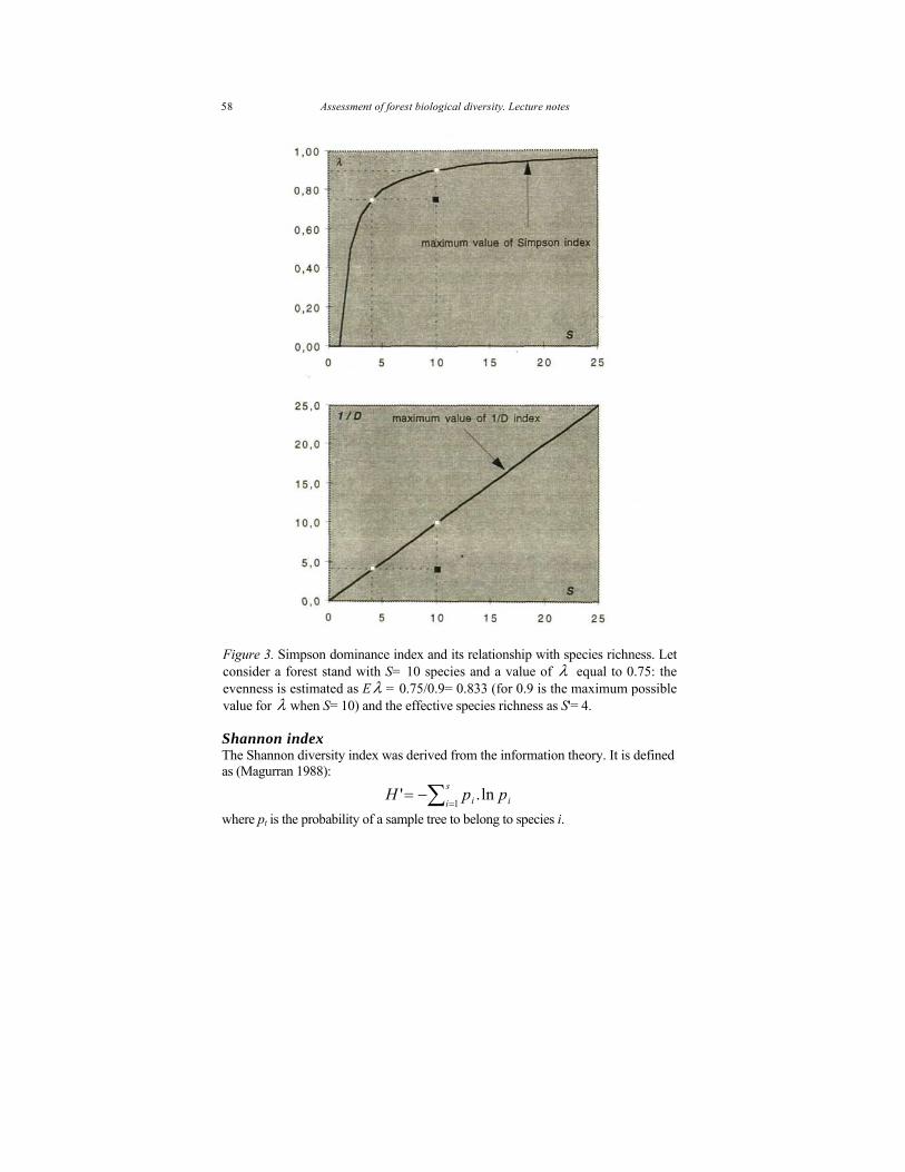
Figure 3. Simpson dominance index and its relationship with species richness. Let consider a forest stand with S= 10 species and a value of λ equal to 0.75: the evenness is estimated as Eλ = 0.75/0.9= 0.833 (for 0.9 is the maximum possible value for λ when S= 10) and the effective species richness as S'= 4.
Shannon index The Shannon diversity index was derived from the information theory. It is defined as (Magurran 1988):
∑ =−=
s
i ii ppH1
ln.'
where pt is the probability of a sample tree to belong to species i.
58 Assessment of forest biological diversity. Lecture notes

Assessing species richness and diversity 59
Because the true value of pi is unknown but estimated, the following formula provides a more rigorous estimate of the Shannon index (Magurran 1988):
H’= -( )
31
21
21
1
1 12
ˆˆ
12
ˆ11ˆln.ˆn
ppn
pn
spps
i iis
i is
i ii∑∑∑ =
−−
=
−
=
−+
−+
−−
where p t =ni/n. In practice, the difference between this estimate and the value derived from the previous formula where pt is replaced by its estimate is very small. A larger source of bias stems from the fact that we do not known S, but only observe a subset of the existing species (Sobs ≤S).
The theoretical variance of the Shannon index is (Magurran 1988):
Var[H’]= 21 1
22
21)ln()(ln
ns
nppps
i
s
i iii −+
−∑ ∑= =
For a given species richness, S, the maximum value of the Shannon's index is obtained when the species distribution is fully even (i.e., pi = 1/S): max( H ′ ) = lnS. This result shows that the maximum value of the index indefinitely increases when species richness increases.
This result can further be used to define an evenness index, which varies between 0 (one-species community) and 1 (all the species have the same frequency): E H ′ = H ′ /lnS. For a given value of H ′ \ it is also possible to determine an effective species richness S" as the number of species which would give the same value of H’ if they were evenly distributed: S"=exp( H ′ ) (1≤S"≤S).
Which sampling design for species diversity?
Most of the guidelines mentioned above for species richness still hold true for diversity. Several points should however be emphasised.
When sample size increases, diversity indexes tend to stabilise much earlier than richness estimates (which, as we saw, never stabilise but steadily increase). The size of the sample can thus be reduced if diversity is the primary concern (in fact, this is the reason why only 400 trees are sampled in Fig. 2).
The diversity indexes are not based on binary data but on the relative abundance of species. Estimates derived from sampling designs where the probability of trees to be included in the sample varies according to tree size (e.g., as in Fig. 2) should thus take this aspect into account. Another related issue is whether the index should be based on the frequency of the individuals or on some other information such as the relative biomass of the species (which may yield very different estimates of diversity, because some species never reach a big size).
Another difficult point concerns the estimation of the frequency of a given species. Such estimates can be precise for most species only if a very large number of individuals is sampled (say, more than 10 000 trees in an evergreen forest which

60 Assessment of forest biological diversity. Lecture notes
may contain some 200 tree species). Even in that case, very rare species may be omitted and the frequency of rare species is poorly estimated.
The Jackknife procedure presented for species richness (§ 3.2.2) can also be applied for diversity indexes (Heltshe & Forrester 1985).
As for species richness, it may be recommended to stratify the sample according to ecological factors —both exogenous (e.g., topography, local changes in site quality) and endogenous (e.g., silvigenetic cycle)—, which influence the partern of species distribution (Pélissier 1997, Gimaret et al 1997). Beside the fact that it has a simple interpretation (the probability that two independent sample individuals do not belong to the same species) and that its maximum value is rapidly bounded, a key advantage of the Simpson index is that it may be broken into additive components when stratified sampling is chosen: it is indeed possible to estimate an average diversity within strata and an across strata diversity (Lande 1996).
References
Chao A. 1987. Estimating the population size for capture-recapture data with unequal catchability. Biometrics, 43: 783-791.
Cochran W.G. 1977. Sampling techniques. 3rd. edition. Wiley & Sons, New York, 413 pp.
Colwell R.K., Coddington J.A. 1994. Estimating terrestrial biodiversity through extrapolation. Phil. Trans. R. Soc. Lond. B, 345: 101-118.
Condit R., Hubbell S.P., Lafrankie J.V., Sukumar R., Manokaran N., Foster R.N., Ashton P.S. 1996. Species-area and species-individual relationships for tropical trees: a comparison of three 50-ha plots. Journal of Ecology, 84: 549- 562.
Gimaret C, Pélissier R., Pascal J.-P. 1996. Assessment and variations of the tree species richness and diversity in a wet evergreen forest of South India. Poster, Symposium Biodiversité et fonctionnement des écosystèmes, Ecole normale supérieure, Paris (12-14/06/96).
Gimaret C, Pélissier R., Pascal J.-P., Houllier F. 1997. Sampling tree species diversity in a dense moist evergreen forest with regard to its structural heterogeneity. Journal of Vegetation Science (accepted).
Gégout J.-C., Houllier F. 1996. Canonical correspondence analysis for forest site classification. A case study. Ann. sc. for., 53: 981-990.
Heltshe J.F., Forrester N.E. 1983. Estimating species richness using the Jackknife procedure. Biometrics, 39: 1-11.
Heltshe J.F., Forrester N.E. 1985. Statistical evaluation of the Jackknife estimate of diversity when using quadrat samples. Ecology, 66 (1): 107-111.

Assessing species richness and diversity 61
Hill M.O. 1973. Reciprocal averaging: an eigenvector method of ordination. J. Ecol., 61: 237-249.
Hurlbert S.H. 1971. The nonconcept of species diversity: a critique and alternative parameters. Ecology, 52: 577-586.
Journel A.G., Huijbregts C. 1978. Mining geostatistics. Academic Press, London, 600 pp.
Lande R. 1996. Statistics and partitioning of species diversity, and similarity among multiple communities. Oikos, 76: 5-13.
Lanly J.-P. 1981. Manual of forest inventory. FAO Forestry Paper, 27, Rome, 200 pp.
Magurran A.E. 1988. Ecological diversity and its measurement. Croom Helm Ltd, London, 179 pp.
Pélissier R. 1997. Hétérogénéité spatiale et dynamique d'une forêt dense humide dans les Ghats occidentaux de l'Inde. Publications du département d'écologie 37, Institut français de Pondichéry, 150 pp.
Pielou E.C 1995. Biodiversity versus old-style diversity: measuring biodiversity for conservation. In T.J.B. Boyle & B. Boontawee (Eds): Measuring and monitoring biodiversity in tropical and temperate forests, CIFOR, Bogor, Indonesia, pp. 5-17.
Sanders H.L. 1968. Marine benthic diversity: a comparative study. Amer. Nat., 102: 243-282.
Scherrer B. 1983. Techniques de sondage en écologie. In S. Frontier (Ed.): Stratégies d'échantillonnage en écologie, Masson, Paris, pp. 63-162.
Ter Braak C.J.F. 1986. Canonical correspondence analysis: a new eigenvector technique for multivariate direct gradient analysis. Ecology, 67: 1167-1179.
Tilman D., Downing J. 1994. Biodiversity and stability in grasslands. Nature, 367: 363-365.
Tilman D., Wedin D., Knops J. 1996. Productivity and sustainability influenced by biodiversity in grassland ecosystems. Nature, 379: 718-720.

62 Assessment of forest biological diversity. Lecture notes
Permanents plots as a means to monitoring forest dynamics and biodiversity
François Houllier
Abstract
With the emphasis shifting from the one-time assessment of forest resources to the continuous monitoring of their changes, the question of installing permanent plots has become more and more acute across the world. This paper reviews some of the problems that arise when permanent plots are set up with the aim to monitor forest biodiversity and/or forest dynamics.
The major advantages of setting permanent plots rather than having successive independent surveys are that (i) this reduces the imprecision in the estimates of change, and (ii) this provides a means to investigate the components of the changes.
However there are several technical issues which always come to the surface and have to be discussed and solved according to the specific context and objectives: - whether the plots should be physically demarcated in the light of the diffusion of global positioning systems (GPS); - the choice between several alternative sampling designs: minimum size of the plot, cluster of plots vs. a single connected plot, network of medium-size plots vs. a few large plots; - the minimum size of the sample trees; - the way changes are estimated if the time step is long.
Introduction
Due to the fast quantitative erosion of forest area in the world and to the qualitative degradation of the remaining forests (e.g., replacement of "natural" closed forests by disturbed open forests or tree plantations), the focus of most forest inventories has shifted from the one-time assessment of forest resources to the continuous monitoring of their changes.

Monitoring forest dynamics and biodiversity 63
In that general context, two complementary approaches are often proposed in order to estimate the ongoing changes: - using remote sensing, mapping and geographic information systems as means to detect, represent and assess the global changes in forest area and the flows from one forest type to another; - installing permanent plots for assessing the local changes in forest biomass and structure, in tree species richness and diversity, and for describing and understanding the processes involved in forest dynamics and maintenance or loss of biodiversity.
This lecture is only concerned with the latter point and discusses some of the technical issues involved when permanent plots are to be laid and monitored. The choice of the sampling design is obviously crucial, for it determines the amount of field work —hence of money to be spent—, as well as the reliability of the estimates. This problem has already been partially discussed during the lectures focusing on the assessment of biodiversity itself: the homogeneity of the forest as well as the level at which diversity is to be estimated are essential. But other interrelated objectives often come into the picture: monitoring the changes in forest composition; assessment and monitoring of volume and biomass; assessment of stand structure and monitoring of its demography.
Several technical issues which always come to the surface are discussed in this lecture: - Whether permanent plots are useful or could be efficiently replaced by successive independent surveys. Whether the plots should be physically demarcated in the light of new technological developments (i.e., the diffusion of Global Positioning Systems (GPS)) and whether the trees should be individualised and mapped. - Whether a few large plots should be preferred to a set of medium size-plots to assess the forest diversity and structure in a vegetation type; whether one single connected plot is preferable to a cluster of satellite plots; the reciprocal advantages and drawbacks of fixed-area and variable-area plots, etc. - The periodicity of measurements and the minimum size for trees to be measured: international guidelines, consequences on diversity estimates, on biometric assessment, on demographic studies.
A statistical point about permanent plots
The major advantages of setting permanent plots rather than having successive independent surveys are that permanent plots: (i) reduce the imprecision in the estimates of change; (ii) provide a means to break global estimates of changes into their components (mortality, growth, recruitment).

64 Assessment of forest biological diversity. Lecture notes
Variance of the estimate of change
Let us take the case in which the same zone is sampled at two successive occasions, t1 and t2, and a single plot is laid down at each point of time. There are three possibilities: (i) the two plots are independent of each other; (ii) the plot is a true permanent plot, i.e., it was clearly marked at t1 so that it is precisely relocated at t2; (iii) the plot is approximately permanent, e.g., the plot was not marked at t1 but is relocated at t2 using GPS technology.
These three cases can be compared within the framework of a single statistical model. Let y be the variable under study and x the coordinates of the plot. The observed values are: y1 = y(x1,t1) and y2 = y(x2,t2). Let us consider the following statistical model which, though arbitrary and simple, seems quite reasonable, at least qualitatively: y is a random function with a known variance, σ2 , and spatial and temporal correlation function, p(δx,δt) = ps(δx).pt(δt), where ps(δx) and pt(δt) are monotonously decreasing functions. We further assume that the coordinates of the
plots are randomly selected. - Vind ≈ 2σ2, - Vappr ≈ 1.2σ2, - Vperm ≈ 0.4σ2.
These results exhibit big differences among the three situations and clearly show the advantage of using a permanent plot, at least an approximate one.
Under this model, it is possible to estimate the variance of the estimated change, yΔ = y2-y1: Var[ yΔ ] = 2σ2 (1-ps( xΔ ) pt( tΔ )) where xΔ = x2-x1 and
tΔ = t2-t1. - If the plots are independently selected from each other, the expected value of this variance is:
Vind = E[Var[ yΔ ]] = 2σ2 .(l –Pt( tΔ ) ∫∫ ps(x2 – x1) dx1 dx2)
Vind = 2σ2 (l - pt ( tΔ ) E[ps (x2 – x1)]) - If the plot is a true permanent plot, the expected value of this variance is:
Vperm = 2σ2 (1- pt( tΔ )) - If the plot is approximately permanent, the expected value of this variance is: Vappr = 2σ2 (l - pt( tΔ ) ∫ ps(ξ ).p(ξ ) d(ξ )
where the integral is taken over the range over possible values of ξ = xΔ and p(ξ ) is its probability distribution function.
It can thus be demonstrated that: Vperm ≤ Vappr ≤ Vind ≤ 2σ2. If we take a reasonable numerical example such as Pt( tΔ )= 0.8, ps(ξ )= exp(-ξ /200) and p(ξ ) = 1
[-200,200] (ξ )/400- and if we suppose that the plots are situated in an area larger than some thousands of hectares, then we get the following approximate values:

Monitoring forest dynamics and biodiversity 65
This advantage has actually been recognised for a long time. But there was some debate on whether estimates derived from permanent plots would be biased, not at t1, but at t2 and subsequent dates. Provided that the sampled domain is always the same, estimates derived from permanent plots are not biased.
It has however been showed that there is an intermediate sampling strategy, called sampling with partial replacement, which: (i) is more efficient than temporary plots for both one-time estimates and change estimates; (ii) is less efficient than permanent plots for change estimates; (iii) is more efficient than permanent plots for one-time estimates. This strategy has been widely presented and reviewed in the field of timber-oriented inventories (e.g., see Houllier 1985) and could probably be adapted in the field of diversity-oriented forest surveys.
One important point that is often overlooked regarding sampling with partial replacement: this strategy, though theoretically efficient, is complicated to put in practice when it comes to operational forest surveys.
Dynamic balance and its components
The primary aim of monitoring is to assess changes. For instance: if we are interested in plant demography and biomass between dates t and t+k, it means estimating the change in the number of stems per ha, tktktt NNN −=Δ ++, or in the basal area, tktktt GGG −=Δ ++, ; if we are interested in species diversity, it means estimating the change in species richness, tktktt SSS −=Δ ++, . As seen above, this can be achieved by various ways (permanent or temporary plots), which may strongly differ in their precision.
But soon after changes have been estimated, the questions arise of how these changes happened, of how they can be broken down into elementary components. Estimates of change then become global balances whose elements have also to be estimated: - )( ,,,,, kttrmkttrmkttmkttrktt NNNNN +++++ −+−=Δ , for the number of stems (see below for the meaning of these notations), - )( ,,,,,, kttrmkttrmkttikttmkttrktt GGGGGG ++++++ −++−=Δ , for basal area,
- )( ,,, kttrmkttrmtmktrktt SSSSS ++++ −+−=Δ , for species richness.
If the plots are not truly permanent and if the trees are not individually tagged, there is no possibility to estimate the various components of these equations (recruitment, mortality, felling, disappearance of species, colonisation by new species) without some additional hypothesis on the relationships between the state of the stand and the changes that happen. Since the very question is often to estimate these relationships, there is no reliable solution in the absence of permanent plots.

66 Assessment of forest biological diversity. Lecture notes
Transversal sampling using age instead of time
One problem with successive surveys, be it with permanent or temporary plots, is that it takes several years before changes can be assessed: thus, the idea to use plots sampled at the same date but situated in different stands ordinated along an age-like gradient. The main difficulty with this approach lies in the fact that the age-like gradient may be correlated to some ecological factors, which have themselves a strong influence on biodiversity or standing stock. This is a very general problem, which also applies to biodiversity studies.
Example: let us consider the coffee plantations in the Coorg District (South India) and their impact on the tree diversity in the canopy. One possible approach is to sample plots in coffee plantations which have a different age. In the case of coffee plantations, it hence turns out that most older plantations are large and are situated in the (former) moist deciduous forest belt, whereas most younger plantations are smaller and result from the encroachment on moist evergreen forests. It is thus difficult to simply interpret the loss of species diversity along the sampled age-gradient as the result of a progressive degradation process when the coffee plantation ages.
Monitoring forest dynamics
Monitoring volume and biomass
The estimation of volume and biomass at one point of time does not pose any major methodological problem. One point that is still often lacking is the existence of adequate volume tables: developing such tables is not complicated but is a tedious job and actually requires a lot of time.
In many national inventories, some procedures have been designed and applied in order to limit the number of small sample trees: for example, relascope plots or concentric fixed-area plots where the smaller trees are sampled only in the smaller plots. These techniques are fine and efficient for estimating volume and biomass at one point of time. However, they generate some difficulties when change is to be assessed: for instance, trees which had been existing for many years suddenly appear in the larger concentric plots because they have grown above the minimum threshold associated to these plots.

Monitoring forest dynamics and biodiversity 67
Monitoring stand structure
The assessment of the size distribution of a forest ecosystem is important in an ecological perspective, for the level of homogeneity / heterogeneity of a stand is generally believed to be linked to its species diversity (not only of trees but also of other plants and of animals). Estimating the frequency of trees in the various size classes does not pose any major problem, except that the estimate of the frequency of bigger trees is often very unprecise (due to their rarity and their more erratic spatial distribution).
Regarding the fixed-area vs. variable area plot debate, the same comments as above hold true when it comes to monitoring the flows of trees from one size class to another.
Comparing two successive diameter distributions, to test the hypothesis of stability between t and t+k, can be simply achieved by a classical Chi2-test.
Characterising the structure of a stand may also mean characterising its vertical structure and the spatial distribution of the trees: - Beside tree height, the former may require the measurement of crown height and width. The usual way to study the vertical structure is to study the relationship between diameter at breast height and stem height. For self-understanding reasons, it is preferable to analyse h-1.3O = f(d1.30) rather than h = f(d1.30), and to consider it on a per species basis rather than all species pooled together. The use of the so- called h = 100 .d line should thus be avoided. - At the moment, characterising the spatial distribution of trees is more a matter of research than of operational forest surveys. The techniques which can be used are varied: hand-drawn or automatic profiles based on stem and crown measurements, statistical analysis of spatial patterns based on the inter-tree distribution (Pélissier 1997). Analysing the changes in spatial distribution is even more complicated.
Monitoring demographic processes
Monitoring demographic processes means breaking the global assessment of change in its different components: mortality, recruitment and growth. As already mentioned, true permanent fixed-area plots, where all trees are identified and tagged, are best suited for that purpose.
Mortality Mortality and survival rates are usually estimated by counting the trees that existed at t and have either died or survived up to date t+k: mNt,t+k. The (relative) rate of mortality is then obtained by dividing this value by the initial density and the time elapsed between the two successive surveys: mNt,t+k/(k . Nt).

68 Assessment of forest biological diversity. Lecture notes
One minor problem may occur when k is high (say, about or more than 10 years). In such a case, a better approach is to consider mortality and survival as fixed annual probabilities: mNt,t+k =m.Nt Simple computations then give an exact estimate of the mortality probability:
k
t
kttm
NN
m /1, )(1~ +−=
which can be approximated by the usual formula given above (if mNt,t+k/Nt « 1). This procedure is also valid if it comes to estimate the transition probabilities from one size-class to the other in the framework of a matrix demographic model.
Recruitment The case of recruitment is slightly different, for it is often assumed to be a fixed annual amount rather than a fixed annual probability. - In the first case, recruitment is simply estimated as the number of trees counted at t+k which had not been counted at t, divided by the time elapsed between the two successive surveys: rNt,t+k/k. - In the second case, recruitment rate can be estimated using the same procedure as for mortality rate.
Another critical feature with recruitment is the threshold size for the trees to be measured: the higher the threshold, the lower the recruitment. Recruitment can thus not be equated to regeneration. Internationally agreed values for this threshold are 1 cm and 10 cm dbh. It is important to stand by these values because this is the only means to ensure the comparability of estimates obtained the world over.
It must further be observed that the above given estimates of recruitment and mortality are both biased, for the trees which were recruited after t and died before t+k are not included. This is not a matter of concern when only a balance is estimated for these two phenomena exactly compensate each other. However, this may pose some problems if two forests, which have been sampled with a very different periodicity, are compared for mortality or recruitment rate.
Turn-over Mortality and recruitment are two aspects of the turn-over of a tree community. In a stable "climacic" forest, it is imagined that these two values are equal. First, one may argue that "climax" never exists and that total stability is a myth. Second, it most often happens that the two values are actually different. Assessing the turn-over rate is then carried out by averaging the mortality and recruitment rate:
2/)ˆˆ(ˆ rm +=τ .

Monitoring forest dynamics and biodiversity 69
Increment Assessing the biological increment of the forest has been widely reviewed and does not pose any major problem when fixed-area permanent plots are used.
The only critical point is with the clear distinction between increment of standing trees and ingrowth (i.e., the volume, basal area or biomass of trees which have crossed the minimum threshold for being recorded): either the increment of recruited trees (after they crossed the threshold) is included in ingrowth, or it is integrated into the overall increment of standing trees.
When variable-area plots are used, the situation becomes more complicated, because this problem of recruitment above a given threshold is amplified.
From assessing changes to understanding processes The points above all deal with how to estimate and assess the changes, either as a global balance, or as elementary demographic components. A subsequent question is often to understand the processes that result in regeneration and in tree growth or death. Answering this question often leads to link these dynamic processes to the environment of the trees and stands at the local level: light availability, site quality, slope, etc.
This domain is more an area of research than an area of operational survey. Permanent plots play here a key role, provided the trees have been mapped and the plots are big enough so as to ensure that the environment of most sample trees is known.
Monitoring species diversity
Assessing species diversity
The main problem is to clearly state at which level species diversity is to be assessed. Let us take two contrasted examples: - If the diversity is to be estimated at the stand or community level (a-diversity and, possibly, β-diversity): the choice will be between a single large plot (say between 5 and 50 ha), a set of a few medium-size plots (say 3 to 5 one-ha plots), a cluster of several small plots (say 20 to 30 twenty-tree plots). - If the diversity is to be estimated at the level of a forest type (γ-diversity): it will be necessary to sample various plots located in different forest patches and stands and the choice will concentrate on the compromise between the number of plots and their size.

70 Assessment of forest biological diversity. Lecture notes
In both cases, it is necessary to state at which scale the estimates of diversity are provided: one ha or the total community, one ha or the total vegetation type.
An important point which actually concerns most operational forest inventories is that they use some form or another of varying-size plots, where larger trees have a higher probability to be sampled. Let p(d) be the probability of a tree of size d to be sampled. The estimates of the standing stock easily take this factor into account, by weighting the observations by the inverse of the probability to be observed. The situation is a bit different for diversity: - for richness, this procedure may result in a bias as soon as there is any form of correlation between species composition and size structure (e.g., some species yielding only small individuals); - for species frequency, the procedure described above can be applied, without any adverse consequence, but the fact that rare small-size species have more chance to be missed.
Monitoring species richness and diversity
Changes in species richness
The first step in assessing changes in species richness over time is fairly similar to the first step in assessing the changes in the standing stock: the estimate of the overall balance is to be estimated; and, as stated in section 2, this estimate is more precise if permanent plots are used than if temporary plots are used.
Then the question comes to estimate the components of this balance: how many new species have appeared and how many have disappeared? This can actually be carried out even if temporary plots are used, which is a major difference from the assessment of the components of changes in the standing stock. But, of course, the estimates do not have the same reliability whether the plots are permanent or temporary.
Other important points are: - that the scale-dependence of diversity may yield paradoxical results. For example, it may happen that changes occurring at plot scale do not appear anymore when all plots are pooled together (Table 1). - that the time step of richness and diversity changes is usually longer than the time step of biomass changes. Of course, this is not the case during some special events such as colonisation of open land, treefall due to heavy storms or massive dieback. It is worth noting that in such cases, the standing stock also dramatically changes.

Monitoring forest dynamics and biodiversity 71
Table 1. Theoretical example where changes in species richness are not "consistent" across spatial scales. Each plot loses and gains one species, but the pooled plots neither gain nor lose species.
Plot 1 1 2 2 1&2 1&2 Time t1 t2 t1 t2 t1 t2
species
s1 1 0 0 1 1 1 s2 1 1 1 1 1 1 s3 0 1 1 0 1 1
Note: such a situation may occur when a forest is composed of a mosaic of silvigenetic patches which, each, undergo the same cycle but are not synchronised.
More important than numbers of species, the lists of the species —those which remained, those which disappeared and those which appeared— help understanding the nature of the changes: for example, whether the species that appeared are light-demanding or tolerant, to which strata they belong, whether they are indicators of disturbance, whether they are deciduous or evergreen, exotic or indigenous.
Changes in species diversity
Changes in diversity indexes can be estimated simply and are, of course, more precise if permanent plots are used. These indexes being composite, it is however difficult to break the changes into components.
Monitoring the changes in diversity means assessing the changes not only in species richness but also in species frequency. To that respect, this is fairly comparable to monitoring changes in the size structure of a stand. For example, comparing two successive species composition can be achieved by a Chi2-test.
Methods discussed for assessing the changes in the overall standing stock can also be applied to single species: for instance, estimate of mortality, recruitment and growth for each species in a stand. One major difficulty in tropical forests is that the high number of species combined with the usual constraints on sampling intensity result in few individuals sampled per species. So that such a species wise approach is rarely feasible.
General discussion
This review has emphasised the usefulness of permanent plots in terms of precision of the estimates of change as well as in terms of possibilities to trace and estimate the components of the changes.

72 Assessment of forest biological diversity. Lecture notes
It has also shown that species richness and diversity, as measures of heterogeneity, of variability, are of a very different nature from volume, biomass, basal area, etc. and that this has several implications on the sampling and estimation processes.
In the field of classical forest inventories, many empirical as well as theoretical studies have shown that, for the same global sample size, the most efficient sampling designs are those which are made of numerous very small plots. When cost and time are taken into account (e.g., cost of travelling from one plot to another), it appears, in temperate forests, that many small plots of, say, 0.01-0.10 ha provide better estimates than a few larger plots. This general guideline can be extended to biodiversity assessment (Gimaret et al. 1996).
A point which is more disputable is about whether the plots should have a fixed size, contain a fixed number of trees, or have a variable size depending on the size of the trees. In the field of classical forest inventories, it is widely accepted that the emphasis should be put on the larger trees which have a higher economic value. However, this choice which results in varying-size plots (e.g., relascope plots) poses some technical problems when it comes to assessing changes or to estimating species richness and diversity.
Furthermore, the question of plot size takes another twist when it comes to monitoring and understanding the dynamic processes that take place. Such an understanding hence often requires to locate the trees in the space, to consider their environment (neighbours, local ecological conditions). In that case, it is much preferable and more efficient to set up large plots where the ratio perimeter / area is small (there are relatively few trees whose neighbours are outside the plot).
It is impossible to propose a unique framework for monitoring biodiversity, but some guidelines may be proposed: - for research purposes, large permanent plots (from 1 to 50 ha) are the best solution; - for operational purposes, clusters (or tracts) of small fixed-area permanent plots are a good solution.

Monitoring forest dynamics and biodiversity 73
References
Gimaret C, Pélissier R., Pascal J.-P. 1996. Assessment and variations of the tree species richness and diversity in a wet evergreen forest of South India. Poster, Symposium Biodiversité et fonctionnement des écosystèmes, Ecole normale supérieure, Paris (12-14/06/96).
Houllier F. 1985. Inventaires successifs en forêt: intérêt théorique et limites pratiques de l'échantillonnage partiellement renouvelé. Ann. Sc. for., 42: 245- 264.
Pélissier R. 1997. Hétérogénéité spatiale et dynamique d'une forêt dense humide dans les Ghâts occidentaux de I'lnde. Publications du département d'écologie 37, Institut français de Pondichéry, 150 pp.

74 Assessment of forest biological diversity. Lecture notes
Indicators of the biological diversity of forests
at the national level: Comments on a French experience
François Houllier
Abstract
This paper reviews the section devoted to biological diversity in an official and public report on indicators of sustainable management of French forests by the French Ministry of Agriculture. This report is taken as an example with the aim of discussing the nature and relevance of several indicators of biological diversity at a regional or national level, as well as to point out some associated methodological problems.
The biological diversity section of this report presents 14 criteria (i.e., groups of indicators) of diversity and sustainability. These criteria may be grouped into three broad classes: - Forest- and ecosystem-oriented indicators: the proportion and nature of mixed forest stands and their change over time; the extent of truly "undisturbed" (or "natural") forests and of "slightly disturbed" forests; the extent of very old even- aged stands which constitute rare and ecologically interesting habitats; the volume of dead wood in forest; the fragmentation of forests in large elementary forest units; the fragmentation of forests in elementary homogeneous and connected forest units; the extent and nature of forest edges and ecotones. - Species-oriented indicators: the list and proportion of indigenous, acclimated and exotic tree species; the list of endangered and/or sensitive species (plants and animals) found in forests; the density of game in forests; the number and area of forests classified for the conservation of genetic resources. - Policy- and management-oriented indicators: the extent (number and area) of national parks and protected forests; the proportion of natural and artificial (i.e., plantation or sowing) regeneration in even-aged highforests; the list of management practices that contribute to forest artificialisation.

Indicators of the biological diversity 75
For each indicator, the way it is estimated as well as its relevance in the context of tropical forests are discussed. This review shows that: (i) assessing the biological diversity of forests requires the combination of many different data sources and viewpoints; (ii) there is a need to explicitly link aggregated and indirect indicators of diversity to ecological functions, forest resources and indicators of sustainability; (iii) many methodological problems persist in the estimation process itself; (iv) these indicators should not be evaluated only once, but monitored through a continuous national forest survey; (v) this report contains indicators which do not fit within the tropical context: therefore, it should not be replicated straightforward but modified and adapted to local conditions.
Introduction
This paper reviews the part devoted to biological diversity in an official and public report published by the French Ministry of Agriculture on indicators of sustainable management of French forests: Les indicateurs de gestion durable des forêts françaises (Anon. 1995). Although other sections of this report also contain information that is important for assessing, monitoring and conserving biological diversity in French forests3, we chose to focus on the section entitled "Biological Diversity" (pp. 27-36) and the associated annexes (pp. 47-49).
This report is taken as an example with the aim to discuss the nature and relevance of biodiversity indicators at a regional or national level, as well as to point out some methodological problems. The objective of this paper is thus to review the 14 biodiversity criteria, and the associated indicators, which are included in this report. Each indicator is defined; the way it is estimated, the sources that are used and its relevance are then discussed per se and in the context of tropical forests. We do not discuss the results themselves because our aim here is not to assess the diversity of French forests but to review methodological aspects.
We chose to group the 14 criteria into three categories: (i) forest-oriented indicators; (ii) species-oriented indicators; (iii) indicators of anthropogenic activities (forest management as well as conservation measures). Although distinguishing between these three groups was not always easy (for example, the extent of forest edges and ecotones is both an ecological characteristic of the forests and a result of human activities), we felt that this classification was useful: the two first categories correspond to the assessment of forests from two complementary points of view —
3 For example: global information on forest resources (area and volume), the history and origins of French forests, global ecological and biogeographical context, forest health or non timber forest products.

76 Assessment of forest biological diversity. Lecture notes
ecosystem-oriented vs. species-oriented —, while the third category contains policy and management-oriented indicators.
Forest-oriented indicators
Proportion and nature of mixed forest stands (§ 4.14)
Indicators. Three types of information are provided: - the extent (in ha and %) of forests according to their level of species mixture: monospecific stands vs. stands containing two, three or more species. - the degree of purity in the stands dominated: for each of 24 major species, the purity of the forest stands (where they dominate) is estimated as the ratio between the volume per ha of the species itself and the total volume per ha (all species pooled together) in the stands where this species dominates. - the changes that occurred between 1984 and 1994.
Source. National Forest Survey: description of forest cover on 0.2 ha field sample plots (determination of which species is dominant) and volume measurements on smaller plots (6, 9 and 15 m radius according to tree size). Comments. The nationale for this criterion seems, at first, evident: mixed stands are more diverse than pure stands. This should however be nuanced: (i) this criterion is scale dependent, for it varies according the size of the stands; (ii) it may happen that a landscape is made of a mosaic of many single-species stands. The way forest mixture is classified in France is not relevant for tropical forests which, except the plantations, are much more diverse (in France, the degree of purity, as defined above, varies between ca. 50 % for some broad-leaved species and more than 90 % for some planted pine stands).
The idea to distinguish between stands according to their degree of species mixture and level of diversity and heterogeneity is however relevant: the difficulty is that such estimates are difficult to derive from aerial photographs or satellite images and thus require direct field observations.
An alternative approach would be to classify and map the forests according to ecological criteria (e.g., soil and bioclimate) and physiognomical aspects that can be directly observed on satellite images or aerial photographs and that are correlated with local forest diversity. An important point is that changes are assessed.
4 For each indicator, we give the number of the paragraph in the French report.

Indicators of the biological diversity 77
Natural and old-growth semi-natural forests (§ 4.2)
Indicators. The extent of natural forests and old-growth semi-natural forests. These forests are respectively defined as highforests which are exclusively composed of indigenous species, have been standing from times immemorial and have been preserved from any harvesting for at least 50 years, and as highforests which are exclusively composed of indigenous species, have not been planted and have been existing for at least 80 years. Sources. National Forest Survey; Forest Department; Ministry of Agriculture. Comments. Such estimates are difficult to establish in European forests which have been strongly modified by human activities over the centuries. So would it be in most Asian tropical countries, at least in those which have a dense population or where shifting cultivation was, and still is, frequent, or where local populations have been collecting non timber forest products for centuries.
Old even-aged stands as rare and specific habitats (§ 4.3)
Indicators. Area covered by very old even-aged stands (i.e. silviculturally overmature stands) for each of 18 major predominant species. Source. National Forest Survey: field sample plots are used. Comments. The rationale for these indicators is that old-growth forests (including some plantations) often constitute specific and rare habitats and harbour a particular fauna and flora.
Such statistics can only be made for regular highforests where age makes sense (e.g., plantations): in France, even-aged stands cover approximately 44 % of the total forest area. In tropical forests, this proportion would probably be less, so that the usefulness of this indicator would be limited. In these forests, at least in those which have no marked dry season, measuring the age may also be difficult.
Volume of dead wood in forest (§ 4.4)
Indicators. Total volume and volume per ha of dead standing trees. Source. National Forest Survey: field sample plots are used; only the trees which died during the 5 years preceding the survey and are still standing are taken into account. Comments The rationale for this indirect indicator is that dead wood provides resources for a wide range of organisms: fungi, insects, insectivorous birds, etc. This indicator is difficult to assess and not very reliable because lying dead wood is not taken into account, the difference between senescent dying trees and dead trees is not always obvious and dating the death of a tree is quite difficult. The task would

78 Assessment of forest biological diversity. Lecture notes
likely be even more complicated in moist and wet tropical forests where the decomposition is more rapid than in temperate forests.
Fragmentation of forest land in elementary geographic units (§ 4.12)
Indicators. An elementary geographic forest unit is defined as a patch of land larger than 4 ha, which contains forest subpatches that are either connected or separated by interruptions (e.g., roads, villages, fields) less than 200 m wide.
The size distribution of elementary forest units is provided, using 7 size classes: [4-100 ha], [100-1000 ha], [1000-5000 ha], [5000-10000 ha], [10000-50000 ha], [50000-100000 ha], more than 100000 ha. For each class, the following additional information are provided: - the average number of forest types per forest unit, which provides an estimate of the average internal diversity within a forest unit; — the average area ( S ), average perimeter ( L ) and average index
of compactness 5)/2( LSπ , average perimeter-over area ratio SL / 6 which characterize the compactness and fragmentation of the forest. Source. The maps prepared by the National Forest Survey from aerial photographs (scale of aerial photographs: 1/17,000; map scale: 1/250,000; minimum size of mapped forest patches: 4 ha; number of broad forest types7: 10). These maps have been put under a GIS and the indicators are directly computed using GIS built-in functions. Comments. The rationale for such indicators is that forest fragmentation is both (i) a major constraint on the natural reproduction and survival of some vegetal and animal species, and (ii) a favourable factor for other species which prefer edges and ecotones (see § 2.7 below). Although the exact ecological meaning of such aggregate indicators is difficult to assess, they are important for conservation purposes and their monitoring may prove useful to evaluate ongoing trends. These indicators also heavily depend on the type of mapping, especially on the scale of the map and the minimum size of the mapped forest patches.
5 This is a shape index which varies between 0 (for a line) and 1 (for a circle). 6 This index mixes patch size and patch shape. 7 The 10 broad forest types are: pure broad-leaved highforest, pure coniferous highforest, mixed highforest, mixture of coppice and broad-leaved highforest, mixture of coppice and coniferous highforest, coppice, parcelled forest, loose forest, forest garrigue or maquis (Mediterranean stunted dry forest with scrub), young plantations and poplar plantations.

Indicators of the biological diversity 79
Fragmentation of forests in homogeneous forest units (§ 4.13)
Indicators. An elementary connected and homogeneous forest unit is defined as a connected patch of forest larger than 4 ha, which belongs to the same forest type.
The size distribution of elementary connected and homogeneous forest units is provided, using 6 size classes: [4-10 ha], [10-25 ha], [25-50 ha], [50-100 ha], [100-500 ha], more than 500 ha.
For each class, the following information is provided: number of units, total area and average area per unit.
The same type of information is also provided for the other wooded lands. Source. The maps prepared by the National Forest Survey from aerial photographs (scale of aerial photographs: 1/17,000; scale: 1/250,000; minimum size of mapped forest patches: 4 ha; number of broad forest types: 10). These maps have been put under a GIS and the indicators are directly computed using GIS built-in functions. Comments. These indicators are complementary to the previous fragmentation indicators. They give an idea of the diversity of ecosystems within the elementary geographic forest units. As for the latter, the ecological meaning of such aggregate indicators is difficult to assess; their monitoring may prove useful to evaluate ongoing trends; they heavily depend on the type of mapping, especially on the scale of the map and the minimum size of the mapped patches.
Using the GIS it would be possible to estimate additional indicators. For example: the size distribution of these units classified per broad forest type (e.g., are there differences between coniferous, broadleaf and mixed highforests?), or the index of compactness of the elementary connected and homogeneous forest units.
Forest edges (§ 4.14)
Indicators. Extent of the interface between forest patches and other land uses: water, humid zones, semi-natural zones (e.g., scrubland, glaciers, alpine grassland), agricultural land, artificial land (e.g., urban areas). The extent of forest edges is given as the percentage of the total perimeter of the forest patches, which are classified according to their size: [4-10 ha], [10-25 ha], [25-50 ha], [50-100 ha], [100-500 ha], more than 500 ha. Source. The land use and forest maps (under GIS) of the French Institute for Environment. Comments. The rationale for such indicators is that edges and ecotones are diversified habitats which harbour a lot of species, either belonging to both neighbour vegetation types, or whose very niche is the forest edge. Analysing the kind of interface between forest and other land uses provides an idea of the potential richness of edges. Analysing the variation according to the size of forest patches
80 Assessment of forest biological diversity. Lecture notes
helps characterising the landscape (e.g., in France, smaller forest patches have more common edges with agricultural land than larger patches, which tend to be more associated with semi-natural land use).
As for the fragmentation indicators, the ecological meaning of such aggregate indexes is difficult to assess; their monitoring may prove useful to evaluate ongoing trends; they heavily depend on the type of mapping, especially on the scale of the map and the minimum size of mapped patches; using GIS functions, it would be possible to go into more details (e.g., looking at the different types of forest and their edges).
Species-oriented indicators
Proportion of indigenous, acclimated and exotic species (§ 4.5)
Indicators. Beside the exhaustive list of the 73 indigenous tree species found in French forests (e.g. fruit trees grown on agricultural land or in orchards are not included), completed by the list of 9 exotic but acclimated tree species (i.e. well adapted to soil and climate, and able to regenerate naturally) and another list of 54 exotic species, the report provides an estimate of the forest area which is dominated by either indigenous or exotic species, in 1984 and 1994. Sources. Experts (botanists) and National Forest Survey. Comments. These lists of species are basic and indispensable indicators, although the distinction between indigenous, acclimated exotic and non acclimated exotic species is not always straightforward. Exotics are not bad per se. They even can increase the apparent richness or diversity of a forest. The problem mainly lies in the fact that their introduction (at the expense of local species) tends to homegenize forests across regions and countries.
The area statistics are not relevant for most mixed tropical forests, which are too diverse to be characterised by a predominant species; for such forests, it is preferable: - either to estimate the area covered by ecofloristic associations as those defined in South India by Pascal (1988); - or to use field survey data to estimate the standing volume or basal area of the species.
Another valuable approach consists in mapping the area over which the species are distributed in order to determine those which have a narrow geographic or ecological niche.

Indicators of the biological diversity 81
Endangered and/or sensitive species found in forests (§ 4.6)
Indicators. Beside a list of rare, endangered or vulnerable plant or animal species found in forests, the report provides the number of species (vascular plants, mammals, birds) found in forests and classified according to their ecological niche (whether they only live in forests or they occasionally move into the forest) and their status (vulnerability, danger of extinction). Sources. Different experts and national or international agencies. Comments. Such indicators are both necessary and very difficult to assess (e.g., what is the ecological niche of a migratory bird species and how much does it depend on forest?). In most cases, it is necessary to consider not only the forests but also the other types of natural, semi-natural and artificial ecosystems required by the species and their populations during their whole life-cycle.
It would also be useful (i) to assess the area of the ecosystems where these species are present, and (ii) to define endangered, rare and sensitive forest ecosystems: but such forest-oriented indicators are difficult to assess on large areas.
Density of game in forests (§ 4.8)
Indicators. Density of Cervidae in forests. Source. Hunting Department, from surveys based on hunting statistics. Comments. The occurrence of large mammals which require a wide and non-fragmented habitat is often a good indicator of the maintenance of large-connected forest patches and of a complete and healthy food webb. This indicator is also provided because hunting is one of the traditional function of French forests: deer density is thus an indicator of a non timber forest resource.
In tropical (and even in temperate) countries, other wildlife animals should be taken into account, such as large mammals (e.g., elephants, tigers) or birds. Many other biological non timber forest resources should also be considered and could lead to the choice of other indicators of biological diversity: medicinal plants, fruits, etc.
Policy-and management-oriented indicators
National Parks and Protected Forests (§ 4.7)
Indicators Extent of different types of protected forests: National Parks, Sanctuaries, Biological Reserves, Hunting Reserves, etc.

82 Assessment of forest biological diversity. Lecture notes
Sources. Ministry of Environment; Ministry of Agriculture; Forest Department (ONF). Comments. These indicators are policy-oriented, rather than descriptive of the existing diversity, and their exact definition and meaning often vary according to countries (see Boontawee et al. 1995 for Thailand). For example, in India, Reserved Forests do not fall under true protected areas but are often better conserved that most other forests.
Forests classified for the conservation of genetic resources (§ 4.9)
Indicators. Number and extent of classified or controlled forest stands, number of genetic inventoried and conserved entities, extent of in situ or ex situ conservation reserves. The distinction between broad-leaved species and conifers is made. Sources. Ministry of Agriculture; Forest Department (ONF); research agencies. Comments. These indicators give an account of the efforts made to conserve species and their genotypes as well as to improve the genetic quality of forest stands (i.e., seeds coming from these classified stands are used in reforestation programmes).
Natural and artificial (i.e., plantation) regeneration in even-aged highforests (§ 4.10)
Indicators. Annual extent of forests concerned by either natural or artificial regeneration; state, communal and private forests are distinguished; afforestation is also included. Sources. Various sources including the Ministry of Agriculture, the National Forest Survey, the Forest Department (ONF), etc. Comments. The rationale for this indicator is that natural regeneration is a better means to conserve the existing tree diversity than planting or sowing. This indicator does not account for the natural regeneration processes which occur in uneven-aged forests (either highforest or coppice-with-standards).
Management practices that contribute to forest artificialisation (§ 4.11)
Indicators. Annual extent of forest stands concerned by "artificial" practices such as ploughing, fertilisation, drainage, and herbicide, insecticide or fungicide treatments; state, communal and private forests are distinguished. Sources. Forest Department (ONF); surveys among private forest owners. Comments. Such indicators give an account of the degree of artificialisation of the forests. They cannot simply be summed up, for some intensively managed forests

Indicators of the biological diversity 83
(e.g., some conifer plantations) cumulate, either the same year or over a rotation, different types of artificial practices. Other indicators, such as the area planted with clones, could also be used. Artificialisation techniques may be different in tropical countries (e.g., shifting cultivation, understorey plantations, slash and burn).
General discussion
Although the above mentioned 14 criteria cover a wide spectrum, they are not exhaustive. For example, other global statistics (e.g., the total forest area, standing volume, current annual volume increment and their changes over a 10-year period), which are important in terms of sustainability and forest conservation, are provided in other sections of the French report. Also it would be relevant to define, and assess the extent of, the vulnerable and rare forest ecosystems; one serious technical difficulty being that such ecosystems may be difficult to directly map from aerial photographs or satellite images.
Assessing the biological diversity of forests at a regional or national level requires the combination of different viewpoints and, thus, of many data sources: the National Forest Survey of course with both their maps and field data, but also administrative information (e.g., National Parks and Sanctuaries), inputs from the Forest Department (ONF) and other organisations in charge of forest management as well as from scientific experts. For example, one of the key question in biodiversity conservation is how to define and characterize the so-called ‘hot spots’. Such areas should harbour a lot of species, preferably indigenous (or better endemics). Also they should be somehow endangered, either because of earlier damages or because of potential threats (e.g., dams, demographic pressure, extension of the agriculture or of communication networks, etc.). Identifying such hot spots thus requires a lot of data species-oriented, stand-oriented, policy-oriented as well as on human activities.
Most of the data provided in this report are indirect and aggregated indicators of biological diversity: there is thus a need for explicitly linking these indicators to ecological functions and forest resources. For example, we generally believe that fragmentation is a negative factor for the conservation of several plant or animal species; but what does an index of compactness of say, 0.2 or 0.8, mean in terms of biodiversity? This has to be explored through detailed and analytical studies that are out of the scope of — but are complementary to — national forest surveys. Similarly, the link of these indicators with the sustainability of forest management is often more intuitive and qualitative than truly demonstrated or quantitatively established.
Beside the latter questions, which are related to the meaning and relevance of the indicators, there are other methodological problems which concern the

84 Assessment of forest biological diversity. Lecture notes
reliability of the procedures used to estimate these indicators. For example, we mentioned that fragmentation and forest edge indexes strongly depend on the mapping technique: the scale and quality of aerial photographs, the forest classification system, the minimum area of patches, the scale of the final map. These technical — often statistical — aspects should not be underestimated in the double perspective of international comparability and national monitoring.
Although the French National Forest Survey started in the early 60s, most indicators provided in this report are static. But we need to assess changes and trends because sustainability is essentially a matter of global time-stability and resilience of forest ecosystems. Therefore, most indicators are not relevant per se, but can provide useful information on ongoing trends in the context of monitoring. It is thus necessary to establish a continuous national or regional forest inventory and to ensure that the method remains consistent over time.
As already pointed out some indicators used in this report cannot be used as such in tropical forests: for example, there is a lack of information on medicinal plants, on other minor or non-timber forest products and on wildlife. But the principles behind these indicators can be used to design criteria which would be better adapted to the tropical context. The book by Pascal (1988) for the South Indian Western Ghats, or the papers by Boontawee et al. (1995) for Thailand and Rollet (1972a, b, c) for Cambodia give some ideas on the way to proceed: - The forest classification system designed by Pascal is based on both ecofloristic (bioclimate, soil and floristic composition) and physiognomic (level of disturbance or degradation, succession stages) criteria. For the evergreen forests alone, he distinguishes 10 climax forest types: this level of detail is justified by (i) the existence of sharp ecological gradients, and (ii) by the "regional" scope of his work. The structure and diversity of the forest types are illustrated by selected plots for which various descriptors are used: height-over-age curve, diameter distribution, vertical architectural profile, list of species, Simpson's and Shannon's index, Importance Value Index. Completed by vegetation maps (scale: 1/250,000) and an atlas of the geographic distribution of endemic tree species, this work provides a consistent framework for assessing the tree and ecological forest diversity across the Ghats. Additional data would nevertheless be required for a more exhaustive assessment of biodiversity: data on other plant species and wildlife, for example. - The forest classification system used in Thailand distinguishes 16 vegetation types: Malayan mixed dipterocarp forest, wet seasonal evergreen forest, lower montane forest, upper montane forest, mixed deciduous with teak forest, mixed deciduous without teak forest, dry evergreen forest, dry dipterocarp forest, dry dipterocarp with pine forest, pine forest, limestone forest, peat swamp forest, beach forest, mangrove forest, bamboo forest, scrub forest. Boontawee et al. (1995) compare these forests using their average density, species richness and Shannon

Indicators of the biological diversity 85
diversity index; however, these information are not derived from a systematic national survey, but from some selected sample forests or plots. - The forest classification System used by Rollet in Cambodia distinguishes 13 broad vegetation types, which are characterised by their most frequent species and a qualitative description of the morphology of the stands, completed by insights in the natural dynamics of these forest types and the succession after disturbances.
References
Anon. 1995. Les indicateurs de gestion durable des forêts françaises. Ministère de l'agriculture et de la pêche, Paris, 49 pp.
Boontawee B., Plengkai C., Kao-sa-ard A. 1995. Monitoring and measuring forest biodiversity in Thailand. In: T.J.B. Boyle & B. Boontawee (Eds), Measuring and monitoring biodiversity in tropical and temperate forests, CIFOR, Bogor, Indonesia, pp. 113-126.
Pascal J.-P. 1988. Wet evergreen forests of the Western Ghats in India: ecology, structure, floristic composition and succession. Institut français de Pondichéry, Travaux de la section scientifique et technique, XXbis, 345 pp.
Rollet B. 1972a. La végétation du Cambodge. Bois et Forêts des Tropiques, 144: 3-15.
Rollet B. 1972b. La végétation du Cambodge. Bois et Forêts des Tropiques, 145: 23-38.
Rollet B. 1972c. La végétation du Cambodge. Bois et Forêts des Tropiques, 146: 3-20.
Iremonger S., Jenkins M., Kapos V., Turner T., Aldrich M., Oldfield S., Reynolds J., Paine J. 1996. Proposais for parameters regarding environmental aspects and the quality of forest resources and forest management for the Forest Resources Assessment 2000. In: Expert consultation on Global Forest Resources Assessment 2000, The Finnish Forest Research Institute, Helsinki, Research Papers 620, pp. 121-159.
Dudley N., Elliott C. 1996. WWF proposals for consideration of forest quality in the temperate and boreal Forest Resource Assessment 2000. In: Expert consultation on Global Forest Resources Assessment 2000, The Finnish Forest Research Institute, Helsinki, Research Papers 620, pp. 160-194.
Mengin-Lecreulx P. 1996. Indicators of suistainable forest management at the national level and possibilities to assess them in national, regional and global forest inventories. In: Expert consultation on Global Forest Resources Assessment 2000, The Finnish Forest Research Institute, Helsinki, Research Papers 620, pp. 195-254.

86 Assessment of forest biological diversity. Lecture notes
Sisk T.D., Lanuer A.E., Switky K.R., Ehrlich P.R. 1994. Identifying Extinction Threats. Global analyses of the distribution of biodiversity and the expansion of the human enterprise. BioScience Vol. 44 (9), pp. 592-604.

Assessing biodiversity and stand structure description 87
Biodiversity assessment and stand structure:
setting up of permanent or temporary plots and
parameters to be studied
Claire Elouard and Rani M. Krishnan
Introduction
Permanent and temporary plots are established for (i) estimation of species richness and diversity on a small scale, (ii) studies of temporal changes in floristic composition and (iii) monitoring ecosystem dynamics.
Before deciding on any of the protocols, the following points should be clearly understood: - the objective for laying a plot or a transect; - availability of funds and manpower; - time available to complete one bout of exercise; - feasibility of extended monitoring capabilities; - data storage and retrieval capacity; - expertise to interpret the available data and assess future experiments.
Two different protocols can be used for data collection: - establishment of permanent plots (fixed-area plots), - laying of temporary plots and transects (plotless method / cluster method).
The objectives of the two protocols are different on the basis of: - temporal need: permanent plots are aimed to address long-term questions related to ecosystem functioning and dynamics; smaller transects or temporal plots are laid to estimate the floristic composition and identify major habitat areas; - spatial data: permanent plots describe and map the trees and vegetation in a systematic way in a defined area; transects provide an estimate of the density and heterogeneity of the vegetation over the sampled area.

88 Assessment of forest biological diversity. Lecture notes
Permanent plots
The main objective for laying permanent plots is to answer questions that only long-term monitoring can provide: ecosystem dynamics and temporal changes in the floristic composition.
Before establishing a permanent plot, the objectives and planning have to be clearly defined: the nature of studies to be carried out in the plot (e.g., biodiversity, phenology, regeneration, recruitment, mortality, recolonisation processes, litterfall and litter decomposition, primary production, architecture, forest mosaic) and the limitations (funds, manpower, time allocated for these studies). The size of the plot, monitoring period and method are then decided based on these criteria.
Size of a permanent plot
An important point that is still unresolved to date is the size of the permanent plots. More precisely, the debate is centered around the question: Do several small plots reflect diversity better than a single large plot?
Several studies have shown that estimates of species diversity and richness are higher when many small plots are sampled, as compared to a few but larger plots (Parsons & Cameron 1974, Routledge 1975, Whitmore 1984, Whitmore et al. 1985). However, large plots also have their advantages: a more diverse representation of life forms; the gradient of species commonality and rarity become apparent; site monitoring of dynamic changes in the ecosystem can be undertaken continuously (Bakker et al. 1996a & b, Herben 1996).
The minimum size for a permanent plot should be 1 hectare. Species diversity and dynamic processes are poorly estimated in plots smaller than this.
Laying of the plot
To lay a plot of 1 ha (100 x 100 m), a compass is used to fix the direction while drawing the boundaries of the square plot. The direction is continuously checked with the compass while the boundary is extended. Poles (pegs) or stones are placed every 10 m using a measuring tape. The total 1 ha plot is progressively divided into subplots of 10 x 10 m and directions of setting the subplots are changed to avoid measuring errors (Fig. 1). The plot is then subdivided into 10 m subplots (or quadrats) with rope and pegs, using tape and compass. If necessary for the study (seedlings count, ground cover, etc.), quadrats of 5 x 5 m are laid within the 10 x 10 m subplots.

Assessing biodiversity and stand structure description 89
Figure 1. Example of progressive setting of a 1 ha plot
Plots are laid using slope correction (Fig. 2): the plot is considered as a plane surface, independent of slope variation. While placing the poles every 10 m, the slope is measured and the distances are corrected to the slope (Table 1).
10 m
Figure 2. Correction of the distance according to the slope (eg.: for a slope of 35°, the distance of 10 m on the map becomes 12.20 m in the field).
Table 1. Slope correction
Slope degree 0 1 2 3 4 5 6 7 8 9
0 1. 00 1. 00 1. 00 1. 00 1. 00 1. 00 1. 01 1. 01 1. 01 1. 01 1 1. 02 1. 02 1. 02 1. 03 1. 03 1. 04 1. 04 1. 05 1. 05 1. 062 1. 06 1. 07 1. 08 1. 09 1. 09 1. 10 1. 11 1. 12 1. 13 1. 143 1. 15 1. 17 1. 18 1. 19 1. 21 1. 22 1. 24 1. 25 1. 27 1. 294 1. 31 1. 33 1. 35 1. 37 1. 39 1. 41 1. 44 1. 47 1. 49 1. 52
Parameters
The monitoring of forest dynamics requires quantifying the following parameters: - Numbering of the trees : All trees more than 30 cm gbh are numbered. The number can be either painted on the trunk or written on a metal label attached to the

90 Assessment of forest biological diversity. Lecture notes
tree. Although painting is cheap, it has to be renewed every year (hence requires manpower). - Spatial location of the trees: The trees are located and mapped within the plot, using a measuring tape to get the x and y coordinates. The coordinates are measured from one corner of the plot, facing North, for each 10 m quadrats and then adjusted for the whole plot. The mapping of trees is necessary for different studies such as stand structure, species and tree distribution, fruit production, seed dispersal and germination, regeneration and recolonisation processes in tree-fall gaps. - Species identification: Species are identified in the field and by herbarium specimens collected from the unidentifiable species. - Girth: Girth at breast height (130 cm) is measured with a measuring meter or with micro-dendrometers (metal ring permanently fixed on the tree trunk). The first method is cheaper, valid only for a one-time measurement of the girth. The second method is preferable if regular monitoring of the tree's growth is required (long term studies). The girth is measured at 130 cm, but if the tree has buttresses, the measurement is taken above the buttresses. - Height: Height is measured with a slope meter: at a defined distance from the tree (15, 20 or 30 m depending on the tree height), the height is measured by the slope meter giving an angle from the top of the crown to a fixed point at the observer's eyes level. A correction is then made with the slope angle from the observer to the tree and the height of the fixed point is added. - Crown diameter: Estimate of crown diameter is necessary to understand spatial development at the canopy level, growth of canopy trees and, finally, the role of tree falls. - Recruitment and regeneration
1) Saplings below 10 cm and above 1 cm gbh are identified, measured (exact measurement or grouped into different height classes, e.g., 25 or 50 cm class intervals) and counted during recruitment studies.
2) Seedlings (<1 cm dbh) are identified, measured (20 or 50 cm class intervals) and counted (number of seedlings of each species within a 5 x 5 m subplot) for regeneration studies. - Intervals between measurements: The time interval between the measurements depends on the objectives.
Assessing the dynamics involves different aspects: 1) long term changes (forest structure, recruitment, floristic changes): this
requires monitoring at low periodicicity, e.g., 5 or 10 year intervals. The measurements are then made for trees >30 cm gbh.
2) survey of mortality and regeneration: this requires monitoring at a high periodicity, e.g., every year or every 2 years. All trees (≥10 cm dbh), saplings (≥lcm dbh) and seedlings (below 1 cm dbh) are measured. Saplings and seedlings

Assessing biodiversity and stand structure description 91
should be monitored on a partial area of the plot in 10 x 10 m subplots for saplings and 5 x 5 m subplots for seedlings, randomly selected within the one-hectare plot.
The turnover for recruitment can be studied yearly or on a long-term basis, depending on the objectives: assessment of global changes over a long period or a continuous survey of regeneration processes and mortality rates. - Terms used to describe the condition of trees in the field:
1) Alive tree - broken alive - fallen but alive - diseased - trunk damaged - debarked - dying 2) Dead tree - dead (unknown causes) - standing dead - dead chablis (gap) - dead broken
-Other measurements: (slope, light, soil temperature, etc.) can be taken during all seasons at different places in the study site.
Examples for permanent plots
First Protocol: Uppangala This experimental station was established in 1990 by the French Institute in the
Kadamakal Reserve Forest in Coorg District, Karnataka, near a small village, Uppangala. This Reserve Forest is situated at the foothills of the Western Ghats. Annual rainfall is about 5 200 mm with a marked dry season of 3-4 months. The experimental station is located at 400-600 m altitude. The natural vegetation is of the Dipterocarpus indicus - Kingiodendron pinnatum - Humboldtia brunonis type of low elevation moist evergreen forest (Pascal 1988). About half the species (48 %) are endemic to the Western Ghats, and about 80 % of the trees belong to these endemic species (Pélissier 1997).
The plot was established within a 28 ha compartment of undisturbed forest (Fig. 3). It comprises three complementary systems, covering more than 5 ha totally: - 5 transects, 20 m wide and 100 m apart, were established to study the floristic composition of the 28 ha compartment; - 3 plots were dedicated to the study of the forest mosaic; - 3 other plots for the specific study of chablis (i.e., tree fall gaps) (Elouard et al. 1996).

92 Assessment of forest biological diversity. Lecture notes
This method is best suited for identifying and monitoring the trees. The shrubs and other life forms were not monitored as rigourously.
Figure 3. Sampling design in the 28 ha undisturbed compartment (from Pélissier 1997).
The five transects (bands A to E) are aimed at providing a good statistical representativity of the whole site: girth structure of the stands, evaluation of species diversity, biometric assessment of the dynamics of the stand (growth, mortality and recruitment). The three rectangular plots (H, R and S) were set up to describe the forest mosaic and its functioning in three topographic situations where the physiognomy of the stand is very different from one another. Finally, four small plots (1, 2, 3 and 4) were established in gaps resulting from chablis, in order to study how a stand evolves following a more or less large opening in the canopy.

Assessing biodiversity and stand structure description 93
Second protocol This protocol was designed to monitor forest diversity and dynamics in the Agastyamalai region, Southern Western Ghats, South India (Ramesh pers. comm.). It involves: - establishment of a one-hectare plot (100 x 100 m), with three replicates for each vegetation type, to study the spatial and floristic structure and dynamics of the forest; - establishment of several smaller plots of 0.01 ha (10 x 1 m) located around each 1 ha permanent plot, in order to capture the structural and floristic variations of the major types. The satellite plots are laid in floristically different or transition types.
Methodology as follows: 1) The one-hectare plot is divided into 10 x 10 m subplots (Fig. 4):
- All individuals with dbh ≥0 cm are measured for height and girth (1 ha); - In addition, all individuals with dbh ≥1 cm are measured for height and girth, in 14 subplots (0.14 ha); - In the same subplots, another smaller plot measuring 5 x 5 m is laid and all individuals with dbh ≤1 cm are measured for the height; heights are classified into 20 cm class intervals (0.035 ha); - For grasses, strobilanthes, bamboos and reeds, the percentage of the area in the covered 5 x 5 m is estimated; - The slopes of the plot are measured and all individuals with dbh ≥10 cm diameter are specially mapped in the one-hectare plot.
2) Measurements taken in the satellite plots: - all individuals with dbh ≥10 cm are identified and measured for girth (100 m2), - in the central 5 x 5 m quadrat of each plot, all individuals with dbh ≥1 cm are identified, measured for girth and counted.
This protocol is applicable to all the floristic variations in a continuum and for all the forest types encountered in the Southern Western Ghats. Further, it also addresses the need to monitor transition forest zones with the help of several satellite plots. The time frame, manpower and budget for such an exercise has to be worked out for each situation based on the working conditions there.

94 Assessment of forest biological diversity. Lecture notes
Figure 4. One-hectare plot with the 14 subplots sampled
Temporary plots (transects)
This method is useful for rapid estimation of diversity and to identify trends in species richness and floristic diversity, and also to identify the crucial areas when sampled along a continuum.
Transects can be used in different ways depending on the objectives, resources and time available:
1) A rapid assessment of the vegetation type and the major species within an area can be done by transects (Fig. 5): a rope is laid over a certain distance (usually 1 km) and all the trees nearest the rope are identified and measured (girth and height). By this method, estimates can be completed within a short period (i.e., in a few hours).
Figure. 5. Rope transect with measurement of the nearest trees

Assessing biodiversity and stand structure description 95
2) Another type of transect also gives a rapid assessment of the vegetation type and tree species in a certain area (Fig. 6): points are made 20-25 m apart along the transect (usually 1 km). All the trees and saplings nearest to these points are identified and measured for girth and height. By this method, large areas can be covered in less than a day.
Figure. 6. Rope transect with radiating measurements
3) Belt transects give an evaluation of the vegetation types, structures and changes. The transect is usually 1 km long (Fig. 7), 20 to 40 m wide (10-20 m on either side of the rope) for tree assessment and depending on the vegetation type (the less dense the wider), and 5 m wide for shrub assessment (2.5 m x 2). All trees with dbh ≥10 cm and poles and saplings with dbh ≥1 cm are identified and measured for girth (and height if desired). Biodiversity assessment has to take shrubs species into account.
Figure. 7. Belt transect
4) The cluster method, elaborated by Gimaret (pers. comm.), has been tested in different vegetation types along the Western Ghats (e.g., evergreen, semi-evergreen, moist deciduous, dry deciduous forests and their degraded types). By this method (Fig. 8) diversity can be assessed quickly (4-5 hours for a vegetation type) and within a large area (1 hectare).

96 Assessment of forest biological diversity. Lecture notes
A square tract is established using a compass. Points are made every 20, 50 or 100 m (according to the forest type) along the boundaries of the square. A total of 20 points are recorded, an then 10 trees of dbh ≥10cm and 10 saplings of dbh ≥1 cm nearest to each of these points are identified.
The following parameters are enumerated for each tree / sapling: - identity of the species, - distance of the tree from the point, - girth at 130 cm, or above buttress if any, - height, - slope angle, - altitude, - other parameters such as crown diameter can be also measured.
Figure 8. Sampling design for assessing forest tree species richness and a-diversity
(Gimaret pers. comm.): rl=distance to the tree, r2=distance to the 10th sapling.
Comparison between the different protocols
General comparison between permanent and temporary plots
Permanent plots and plotless methods have their present advantages and disadvantages (Table 2). Permanent plots enable the study of biodiversity as well as ecosystem dynamics, whereas plotless methods do not permit a continuous study of the ecosystem dynamics nor do they facilitate mapping. The scientific scope of these two methods is not only varied but there is also a vast difference in their demand for resources (finance and manpower). A permanent plot requires well planned long-term research programmes and investment.

Assessing biodiversity and stand structure description 97
Table 2. Comparison between permanent plot and plotless methods
Measure Permanent plot method Plotless method Advantages Disadvantages Advantages Disadvantages
Systematic Oversarnpling of Large area (1 ha) can Assumes that sampling in a an area be sampled in a species occurence & restricted area short time density are random possible processes
Biodiversity Species turnover & Extrapolations to Provides rapid Does not explain transitions over be made with estimate of the causes for the similar extreme care and diversity. observed richness environments with severe Extremely useful and density
limitations method for Preliminary surveys
Data collected can Trends in spatial Data not verifiable be verified. heterogeneity of Represented over a speciation (species known spatial and richness & temporal scale, diversity) can be possible to map, understood verify and measurethe ecosystemdynamics Progressive changes Masks the site-in the ecosystem, specificsuccession & peculiaritiesspecies associations
Ecosystem Processes No precisecomparable across quantification is
dynamics ecosystems & applicable whenhabitats compared across
ecosystemsCan be linked to Simplification, Ecosystem dynamics global processes leading to cannot be monitored in detail
masking ofpopulation &individuals in theprocess
Precise role of predation,
competition, evolutionary strategies can bedefined Experimentation &response of ecosystem can bequantified Microprocesses likegenetic diversity &mating patterns canbe spatially &temporally monitored Can help in longterm conservation
goals

98 Assessment of forest biological diversity. Lecture notes
Establishment of permanent plots: case study Uppangala
The experimental station at Uppangala, (Fig. 3) is a series of bands (or transects) and plots established with different perspectives. In all these compartments, trees with girth exceeding 30 cm gbh were spatially located and botanically identified to the species level. The trees were fitted with microdendrometers and girth measurements have been systematically recorded annually since 1990.
Various studies were conducted in this experimental station (Table 3). The overall objective is to get a holistic view of the forest biodiversity, structure and dynamics, that will ultimately help in formulating management guidelines for this area which contains a large number of endemic species, but whose survival is threatened by increasing human pressure (Elouard et al. 1996).
Table 3. Activities conducted in the Uppangala experimental station
Data unit Relevant phenomenon! Samples Species identification biodiversity, forest structure bands & plotsGirth and height of trees biodiversity, forest dynamics. bands & plots gbh ≥ 30cm forest structure Girth and height of saplings biodiversity, forest dynamics selected plots height ≥ 2m forest structure Orientation & slope angle topography mapping bands & plots Light measurements forest mosaic plotsCrown description forest mosaic plots Systematic sampling of litterfall forest dynamics (primary bands & plots (100 baskets
production, litterfall and over 1 ha) decomposition) Vegetative & reproductive forest dynamics (phenology) bands & plots (91 species; phenology 500 individuals)Observation of mortality forest dynamics bands & plots Regeneration & establishement forest dynamics chablis plotsprocesses in tree-fall gaps Soil seed bank forest dynamics plots Tree architecture forest dynamics bands & plots forest structure Atmospheric pollen: traps, soil forest dynamics (palynology) bands & plotssurface samples & spider webs
Cluster (temporary) method: study of coffee-based agroforestry systems
The plotless method used to analyse the structure and dynamics of the canopy cover of coffee-based agroforestry systems is the protocol shown in Fig. 8. The canopy cover maintains a more or less constant temperature and humidity for the coffee plants underneath. Trees for the canopy cover are therefore chosen to function not

Assessing biodiversity and stand structure description 99
only as shading-providers but also for their economic viability for the plantation (timber, fruits, etc.).
The plotless method was followed to assess species richness and diversity, and also the structure and dynamics of the canopy cover. The tree species were then identified, and measured for the girth, height, crown and their distance from the fixed points. The following studies were then conducted: - species richness (number of species, Chao estimator), - species diversity (Simpson and Shannon-Wiener indices), - stand density (number of stems / hectare), - basal area, - canopy structure: origin of the species (local or exotic), height of the canopy, biomass, - population dynamics: evolution of the population with respect to its present diversity and composition (past, present and future trees), - management practices: commercial and non-commercial uses of the species, regeneration techniques, pruning, etc.
How permanent plots are used to measure temporal changes in vegetation dynamics
Case study: chablis
Recolonisation processes in chablis (gaps resulting from tree fall) is being studied in the Uppangala experimental station. Three plots were established with this objective (Fig. 3) as follows: - demarcating the study area: the gap caused by the fall of the tree(s) was demarcated including a part (10 to 20 m) of the surrounding original forest which contributes to the recolonisation processes (dissemination, recruitment, canopy cover); - laying of the plot: the area was then demarcated with ropes and divided into subplots of 10 x 10 m. Each subplot was further subdivided into 5 x 5 m sample plots; slope was measured for slope corrections (Table 1); - all trees with gbh ≥30 cm were identified, numbered (painted on the trunk) and measured (girth and height); - all saplings with gbh ≥3 cm were identified, numbered (labelled) and measured (girth and height); - seedlings were identified, grouped for each species and measured (0-50 cm, 50-1 m, 1-1.50 m, 1.50-2 m height classes); - coordinates of trees with gbh ≥30 cm were plotted to scale;

100 Assessment of forest biological diversity. Lecture notes
- saplings and seedlings were located within the 5 x 5 m subplots; - slope was measured for mapping topography - light was measured.
The measurements are recorded annually, after the monsoon season, for trees and saplings; seedlings are counted twice a year (before the monsoon, following the dry season, and after the monsoon) for survival studies.
In this context, the following analysis can be undertaken at spatial and temporal levels: - regeneration processes: (i) seedling population and survival rates; (ii) species richness and diversity; and (iii) evolution of the composition of seedling and sapling stands. This leads to a better understanding of dispersal strategies, adaptability and competitive abilities of the species, species specific requirements for optimum growth and development - recolonisation processes: (i) establishment of pioneer and light-demanding species; (ii) stages and strategies of climax forest species and their entry. - impact of chablis on the original forest: (i) development of secondary chablis (tree falls caused by the fall of the first tree, due to damage to the trees or uprooting); (ii) changes in floristic composition and structure of the original forest.
Case study: comparison of disturbed and undisturbed forests in the Uppangala experimental station
A comparative study between disturbed and undisturbed moist evergreen forests was conducted in the Uppangala experimental station (Elouard et al. 1996): - Disturbed forest: 14 plots of 600 m2 each were established in 1985 in a forest which had been exploited selectively in 1979 (8.5 trees felled per ha, logs being hauled by elephants) and which had been partly burnt. The plots were surveyed three times, in 1985-86, 1987-88, 1989-90. - Undisturbed forest: the study was conducted in the network described in § 1.4. - All trees with gbh ≥30 cm were spatially located and botanically identified at the species level,
The measurements recorded were: - girth at 130 cm (gbh) of trees with gbh ≥30 cm; - total height, spread and length of the crown of trees with gbh ≥30 cm; - total height of saplings ≥ 2 m high.
Comparison between the two stands (Laborde 1994, Pélissier et al. submitted) confirmed that a single low-damage — logs were hauled by elephants — selective exploitation does not greatly alter the forest structure and diversity, and that the recovery in biomass and basal area is fairly rapid (Table 4), with a strong stimulation of individual growth (Fig.9). However it suggested that repetition of such harvesting might have a strong long term impact on the forest composition and

Assessing biodiversity and stand structure description 101
dynamics: commercially interesting emergent and upper canopy species would be replaced by understorey species.
Table 4. Density and basal area balance in undisturbed and once-logged compartments. Minimum gbh = 30 cm (from Elouard et al. 1996).
Initial Final Mortality Recruit- Growth Balance state state ment (ha-1) (ha-1) (ha-1. yr-1) (ha-1. yr-1) (ha-1. yr-1) (%.yr-1)
Once-logged compartment A - Sampled area: 0.6 ha - Period: 1986-1993 Density (stems) 578 617 5.0 10.5 - +0.95 Basal area (m2) 34.8 38.8 0.40 0.10 0.86 +1.61
Unlogged compartment B - Sampled area: 3.12 ha - Period: 1990-1994 Density (stems) 606 619 5.2 8.5 - +0.54 Basal area(m2) 39.3 41.0 0.26 0.07 0.59 +1.02
Note: mortality and recruitment were assessed once, at the end of the period of study.

102 Assessment of forest biological diversity. Lecture notes
References
BakkerJ.P., Willems J. H. & Zobel M. 1996a. Long term vegetation dynamics: Introduction. Journal of Vegetation Science, 7: 146-147.
Bakker J.P., Willems J. H. & Zobel M. 1996b. Why do we need permanent plots in the study of long term vegetation dynamics? Journal of Vegetation Science, 7: 147-156.
Elouard C., Houllier F., Pascal J.-P., Pélissier R., Ramesh B.R. 1996. Dynamics of the dense moist evergreen forests - Long term monitoring of an experimental station in Kodagu District (Karnataka, India). Pondy Paper in ecology, 1, Institut Français de Pondichéry, 23p.
Herben T. 1996. Permanent plots as tools for plant community ecology. Journal of Vegetation Science, 7: 195-202.
Laborde H. 1994. Forêts sempervirentes des Ghâts occidentaux : bilan dynamique. Mémoire de fin d'étude, Mastère de sciences forestières, ENGREF (Nancy) & Institut français de Pondichéry, 82 pp.
Parsons R. F. & Cameron D. G. 1974. Maximum plant species diversity in terrestrial communities. Biotropica, 6: 202-3.
Pascal J.-P. 1988. Wet evergreen forests of the Western Ghats in India: ecology, structure, floristic composition and succession. Travaux de la section scientifique et technique, 20bis, Institut français de Pondichéry, 345 pp.
Pélissier R. 1997. Hétérogénéité spatiale et dynamique d'une forêt dense humide dans les Ghats occidentaux de l'Inde. Publications du département d'écologie 37, Institut français de Pondichéry, 150 pp.
Pélissier R., Pascal J.-P., Houllier F., Laborde H. (submitted). Impact of selective logging on the dynamics of a low elevation moist evergreen forest in the Western Ghats (South India). Forest Ecology and Management.
Routledge R.D. 1979. Diversity indices: which ones are admissible. Journal of theoretical Biology 76: 503-515.
Whitmore T. C. 1984. Plant species diversity in tropical rain forests. Biology international special issue, 6: 5-7.
Whitmore T. C., Peralla R. & Brown K. 1985. Total species count in a Costa Rican tropical rain forest. Journal of Tropical ecology, 1: 375-378.

The Institut français de Pondichéry is an autonomous research organisation under the umbrella of the cultural and scientific wing of the French Ministry of Foreign Affairs. Its scope is: "Indian civilisation, history and society. Ecology, environment and development in South and South East Asia".
The Institute is organised in three Departments - Ecology, Indology and Social Sciences -, each having their own series of publications. In addition, the Institute publishes two series of working papers: the "Pondy Papers in Social Sciences" (since 1988) and the "Pondy Papers in Ecology" (since 1997).
Recent publications related to botany, ecology and forestry:
Buchy M. 1996. Teak and Arecanut. Colonial State, Forest and People in the Western Ghats (South India) 1800-1947. Publications du département de sciences sociales, 2, 255 pp. [co-edited with the Indira Gandhi National Centre for the Arts, New Delhi].
Elouard C, Houllier F., Pascal J.-P, Pélissier R., Ramesh B.R. 1997. Dynamics of the dense moist evergreen forests. Long term monitoring of an experimental station in Kodagu District (Karnataka, India). Pondy Papers in Ecology, Institut français de Pondichéry, 1, 23 pp.
Houllier F., Caraglio Y., Durand M. Modelling tree architecture and forest dynamics. A research project in the dense moist evergreen forests of the Western Ghats (South India). Pondy Papers in Ecology, 2, 37 pp.
Kalam M.A. 1996. Sacred Groves in Kodagu Distnct (South India). A Socio-Historical Survey. Pondy Papers in Social Sciences, 21, 53 pp.
Pascal J.-P, Ramesh B.R. 1996. Forest map of South India (1/250,000). Notes on the sheet Bangalore-Salem. Publications du département d'écologie, Hors série 21, 66 pp.
Prabakhar R., Pascal J.-P 1996. Map of the Nilgiri Biosphere Reserve (1/100,000): land use and vegetation. Publications du département d'écologie, sheets n° 1, 2 & 3.
Tissot C, Chikhi H., Nayar T.S. 1994. Pollen of the wet evergreen forests of the Western Ghats, India. Publications du département d'écologie, 35, 133 pp., 75 pl.
Pascal J.-P, Ramesh B.R. 1997. Atlas of endemic evergreen tree species of the Western Ghats. Publications du département d'écologie, 38, 403 pp., 352 pl.
Pélissier R. 1997. Structure spatiale et dynamique des forêts denses humides dans les Ghats occidentaux (Inde). Publications du département d'écologie, 37, 148 p.
Forthcoming:
Ramesh B.R., Franceschi (de) D., Pascal J.-P. Forest map of South India (1/250,000). Trivandrum sheet. Publications du département d'écologie.
Houllier F., Rani M. Krishnan, Elouard C. (Eds). Assessment of forest biological diversity. A FAO training course. 1. Lecture notes. Pondy Papers in Ecology, 4.