assessment of evaluation methods for prediction and...
TRANSCRIPT

Assessment of Evaluation Methods for Prediction and Classification of Consumer Risk in the Credit Industry
Satish Nargundkar and Jennifer Lewis Priestley*
Department of Management and Decision Sciences,
J. Mack Robinson College of Business Administration, Georgia State University 35 Broad Street, Atlanta, GA 30303 U.S.A.

ABSTRACT
In this chapter, we examine and compare the most prevalent modeling techniques in the credit industry, Linear Discriminant Analysis, Logistic Analysis and the emerging technique of Neural Network modeling. K-S Tests and Classification Rates are typically used in the industry to measure the success in predictive classification. We examine those two methods and a third, ROC Curves, to determine if the method of evaluation has an influence on the perceived performance of the modeling technique. We found that each modeling technique has its own strengths, and a determination of the “best” depends upon the evaluation method utilized and the costs associated with misclassification. Subject Areas: Model Development, Model Evaluation and Credit Scoring.
2

INTRODUCTION
The popularity of consumer credit products represents both a risk and an opportunity for
credit lenders. The credit industry has experienced decades of rapid growth as
characterized by the ubiquity of consumer financial products such as credit cards,
mortgages, home equity loans, auto loans and interest-only loans, etc. In 1980, there was
$55.1 billion in outstanding unsecured revolving consumer credit in the U.S. In 2000, that
number had risen to $633.2 billion. However, the number of bankruptcies filed per 1,000
U.S. Households increased from 1 to 5 over the same period1.
In an effort to maximize the opportunity to attract, manage, and retain profitable
customers and minimize the risks associated with potentially unprofitable ones, lenders
have increasingly turned to modeling to facilitate a holistic approach to Customer
Relationship Management (CRM). In the consumer credit industry, the general
framework for CRM includes product planning, customer acquisition, customer
management and collections and recovery (Figure 1). Prediction models have been used
extensively to support each stage of this general CRM strategy.
Figure 1: Stages of Customer Relationship Management in Credit Lending
Customer Management
Target Marketing Response Models Risk Models
Customer Behavioral Models Usage Models Attrition Models Activation Models
Collections Recovery Models
Product Planning
Customer Acquisition
Other Models Segmentation Models Bankruptcy Models Fraud Models
Collections/Recovery
Creating Value
3

For example, customer acquisition in credit lending is often accomplished through model-
driven target marketing. Data on potential customers, which can be accessed from credit
bureau files and a firm’s own databases, is used to predict the likelihood of response to a
solicitation. Risk models are also utilized to support customer acquisition efforts through
the prediction of a potential customer’s likelihood of default. Once customers are
acquired, customer management strategies require careful analysis of behavior patterns.
Behavioral models are developed using a customer’s transaction history to predict which
customers may default or attrite. Based upon some predicted value, firms can then
efficiently allocate resources for customer incentive programs or credit line increases.
Predictive accuracy in this stage of customer management is important because effectively
retaining customers is significantly less expensive than acquiring new customers.
Collections and recovery is a critical stage in a credit lender’s CRM strategy, where
lenders develop models to predict a delinquent customer’s likelihood of repayment. Other
models used by lenders to support the overall CRM strategy may involve bankruptcy
prediction, fraud prediction and market segmentation.
Not surprisingly, the central concern of modeling applications in each stage of CRM is
improving predictive accuracy. An improvement of even a fraction of a percent can
translate into significant savings or increased revenue. As a result, many different
modeling techniques have been developed, tested and refined. These techniques include
both statistical (e.g., Linear Discriminant Analysis, Logistic Analysis) and non-statistical
(e.g., Decision Trees, k-Nearest Neighbor, Cluster Analysis, Neural Networks) techniques.
Each technique utilizes different assumptions and may or may not achieve similar results
with the same data. Because of the growing importance of accurate prediction models, an
entire literature exists which is dedicated to the development and refinement of these
4
models (Atiya, 2001; Richeson et al., 1994; Vellido et al., 1999). However, developing
the model is really only half the problem.
Researchers and analysts allocate a great deal of effort to the development of prediction
models to support decision-making. However, too often insufficient attention is allocated
to the tool(s) used to evaluate the model(s) in question. The result is that accurate
prediction models may be measured inappropriately based upon the information available
regarding classification error rate and the context of application. In the end, poor
decisions are made because an incorrect model was selected, using an inappropriate
evaluation method.
This chapter addresses the dual issues of model development and evaluation. Specifically,
we attempt to answer the questions, “Does model development technique impact
prediction accuracy?” and “How will model selection vary with the selected evaluation
method?” These questions will be addressed within the context of consumer risk
prediction – a modeling application supporting the first stage of a credit lender’s CRM
strategy, customer acquisition. All stages of the CRM strategy need to be effectively
managed to increase a lender’s profitability. However, accurate prediction of a customer’s
likelihood of repayment at the point of acquisition is particularly important because
regardless of the accuracy of the other “downstream” models, the lender may never
achieve targeted risk/return objectives if incorrect decisions are made in the initial stage.
Therefore, understanding how to develop and evaluate models which predict potential
customers to be “good” or “bad” credit risks is critical to managing a successful CRM
strategy.
5

The remainder of the chapter will be organized as follows. In the next section, we give a
brief overview of three modeling techniques for prediction in the credit industry. Since
the dependent variable of concern is categorical (e.g., “good” credit risk versus “bad”
credit risk), the issue is one of binary classification. We then discuss the conceptual
differences among three common methods of model evaluation and rationales for when
they should and should not be used. We illustrate model application and evaluation
through an empirical example using the techniques and methods described in the chapter.
Finally, we conclude with a discussion of our results and propose concepts for further
research.
COMMON MODELING TECHNIQUES
As mentioned above, modeling techniques can be roughly segmented into two classes:
statistical and non-statistical. The first technique we utilized for our empirical analysis,
linear discriminant analysis (LDA), is one of the earliest formal modeling techniques.
LDA has its origins in the discrimination methods suggested by Fisher (1936). Given its
dependence on the assumptions of multivariate normality, independence of predictor
variables, and linear separability, LDA has been criticized as having restricted
applicability. However, the inequality of covariance matrices, as well as the non-normal
nature of the data, which is common to credit applications, may not represent critical
limitations of the technique (Reichert et al., 1983). Although it is one of the simpler
modeling techniques, LDA continues to be widely used in practice.
The second technique we utilized for this paper, logistic regression analysis, is considered
the most common technique of model development for initial credit decisions (Thomas et
6

al., 2002). For the binary classification problem (i.e., prediction of “good” versus “bad”),
logit analysis takes a linear combination of the descriptor variables and transforms the
result to lie between 0 and 1, to equate to a probability.
Where LDA and logistic analysis are statistical classification methods with lengthy
histories, neural network-based classification is a non-statistical technique, which has
developed as a result of improvements in desktop computing power. Although neural
networks originated in attempts to model the processing functions of the human brain, the
models currently in use have increasingly sacrificed neurological rigor for mathematical
expediency (Vellido et al., 1999). Neural networks are utilized in a wide variety of fields
and in a wide variety of applications, including the field of finance and specifically, the
prediction of consumer risk. In their survey of neural network applications in business,
Vellido et al. (1999) provide a comprehensive overview of empirical studies of the
efficacy of neural networks in credit evaluation and decisioning. They highlight that
neural networks do outperform “other” (both statistical and non-statistical) techniques, but
not consistently. However, in Vellido et al. (1999), and many other papers which compare
modeling techniques, significant discussion is dedicated to the individual techniques, and
less discussion (if any) is dedicated to the tool(s) used for model evaluation.
METHODS OF MODEL EVALUATION
As stated in the previous section, a central concern of modeling techniques is an
improvement in predictive accuracy. In customer risk classification, even a small
improvement in predictive accuracy can translate into significant savings. However, how
can the analyst know if one model represents an improvement over a second model? The
7

extent to which improvements are detected may change based upon the selection of the
evaluation method. As a result, analysts who utilize prediction models for binary
classification, have a need to understand the circumstances under which each evaluation
method is most appropriate.
In the context of predictive binary classification models, one of four outcomes is possible:
(i) a true positive – e.g., a good credit risk is classified as “good”; (ii) a false positive –
e.g., a bad credit risk is classified as “good”; (iii) a true negative – e.g., bad credit risk is
classified as “bad”; (iv) a false negative – e.g., a good credit risk is classified as “bad”.
The N-class prediction models are significantly more complex and outside of the scope of
this paper. For an examination of the issues related to N-class prediction models, see
Taylor and Hand (1999).
In principle, each of these outcomes would have some associated “loss” or “reward”. In a
credit lending context, a true positive “reward” might be a qualified person obtaining a
needed mortgage with the bank reaping the economic benefit of making a correct decision.
A false negative “loss” might be the same qualified person being turned down for a
mortgage. In this instance, the bank not only has the opportunity cost of losing a good
customer, but also the possible cost of increasing its competitor’s business.
It is often assumed that the two types of incorrect classification – false positives and false
negatives – incur the exact same loss (Hand, 2001). If this is truly the case, then a simple
“global” classification rate could be used for model evaluation.
8
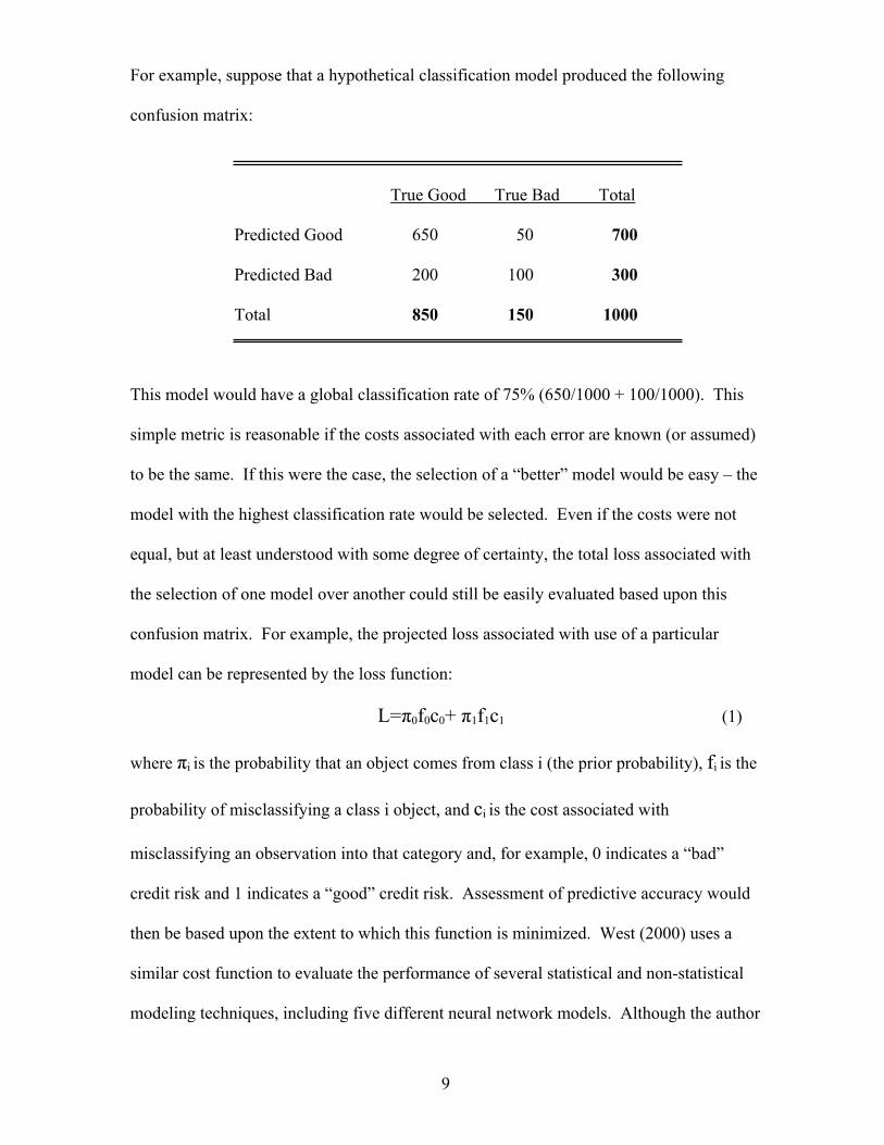
For example, suppose that a hypothetical classification model produced the following
confusion matrix:
True Good True Bad Total
Predicted Good 650 50 700
Predicted Bad 200 100 300
Total 850 150 1000
This model would have a global classification rate of 75% (650/1000 + 100/1000). This
simple metric is reasonable if the costs associated with each error are known (or assumed)
to be the same. If this were the case, the selection of a “better” model would be easy – the
model with the highest classification rate would be selected. Even if the costs were not
equal, but at least understood with some degree of certainty, the total loss associated with
the selection of one model over another could still be easily evaluated based upon this
confusion matrix. For example, the projected loss associated with use of a particular
model can be represented by the loss function:
L=π0f0c0+ π1f1c1 (1)
where πi is the probability that an object comes from class i (the prior probability), fi is the
probability of misclassifying a class i object, and ci is the cost associated with
misclassifying an observation into that category and, for example, 0 indicates a “bad”
credit risk and 1 indicates a “good” credit risk. Assessment of predictive accuracy would
then be based upon the extent to which this function is minimized. West (2000) uses a
similar cost function to evaluate the performance of several statistical and non-statistical
modeling techniques, including five different neural network models. Although the author
9

was able to select a “winning” model based upon reasonable cost assumptions, the
“winning” model would differ as these assumptions changed.
A second issue when using a simple classification matrix for evaluation is the problem
that can occur when evaluating models dealing with rare events. If the prior probability of
an occurrence is very high, a model would achieve a strong prediction rate if all
observations were simply classified into this class. However, when a particular
observation has a low probability of occurrence (e.g., cancer, bankruptcy, tornadoes, etc.),
it is far more difficult to assign these low probability observations into their correct class.
The difficulty of accurate class assignments of rare events is not captured if the simple
global classification is used as an evaluation method (Gim, 1995). Because of the issue of
rare events and imperfect information, the simple classification rate should very rarely be
used for model evaluation. However, as Berardi and Zhang (1999) indicated, a quick scan
of papers which evaluate different modeling techniques will reveal that this is the most
frequently utilized (albeit weakest due to the assumption of perfect information) method
of model evaluation.
One of the most common methods of evaluating predictive binary classification models in
practice is the Kolmogorov-Smirnov statistic or K-S test. The K-S test measures the
distance between the distribution functions of the two classifications (e.g., good credit
risks and bad credit risks). The score which generates the greatest separability between
the functions is considered the threshold value for accepting or rejecting a credit
application. The predictive model producing the greatest amount of separability between
the two distributions would be considered the superior model. A graphical example of a
K-S test can be seen in Figure 2. In this illustration, the greatest separability between the
10

two distribution functions occurs at a score of approximately .7. Using this score, if all
applicants who scored above .7 were accepted and all applicants scoring below .7 were
rejected, then approximately 80% of all “good” applicants would be accepted, while only
35% of all “bad” applicants would be accepted. The measure of separability, or the K-S
test result would be 45% (80%-35%).
Figure 2: K-S Test Illustration
0%
20%
40%
60%
80%
100%
0.00 0.10 0.20 0.30 0.40 0.50 0.60 0.70 0.80 0.90 1.00
Score Cut Off
Cum
ulat
ive
Perc
enta
ge
of O
bser
vatio
ns
Good Accounts
Bad Accounts
Greatest separation of distributions occurs at a score of .7.
Hand (2002) criticizes the K-S test for many of the same reasons outlined for the simple
global classification rate. Specifically, the K-S test assumes that the relative costs of the
misclassification errors are equal. As a result, the K-S test does not incorporate relevant
information regarding the performance of classification models (i.e., the misclassification
rates and their respective costs). The measure of separability, then becomes somewhat
hollow.
In some instances, the researcher may not have any information regarding costs of error
rates, such as the relative costs of one error type versus another. In almost every
circumstance, one type of misclassification will be considered more serious than another.
11
However, a determination of which error is the more serious is generally less well defined
or may even be in the eye of the beholder. For example, turning to the field of medicine,
is a “worse” mistake a false negative, where a diseased individual is told they are healthy
and therefore may not seek a needed treatment, or a false positive, where a healthy
individual is told they have a disease that is not present and seek unnecessary treatment
and experience unnecessary emotional distress? Alternatively, in a highly competitive
business environment is a worse mistake to turn away a potentially valuable customer to a
competitor, or to accept a customer that does not meet financial expectations? The
answers are not always straightforward and may vary with the perceptions of the evaluator.
As a result, the cost function outlined above, may not be applicable.
One method of evaluation, which enables a comprehensive analysis of all possible error
severities is the ROC curve. The “Receiver Operating Characteristics” curve was first
applied to assess how well radar equipment in WWII distinguished random interference or
“noise” from the signals which were truly indicative of enemy planes (Swets et al., 2000).
ROC curves have since been used in fields ranging from electrical engineering and
weather prediction to psychology and are used almost ubiquitously in the literature on
medical testing to determine the effectiveness of medications. The ROC curve plots the
sensitivity or “hits” (e.g., true positives) of a model on the vertical axis against
1-specificity or “false alarms” (e.g., false positives) on the horizontal axis. The result is a
bowed curve rising from the 45 degree line to the upper left corner – the sharper the bend
and the closer to the upper left corner, the greater the accuracy of the model. The area
under the ROC curve is a convenient way to compare different predictive binary
classification models when the analyst or decision maker has no information regarding the
costs or severity of classification errors. This measurement is equivalent to the Gini index
12
(Thomas et al., 2002) and the Mann-Whitney-Wilcoxon test statistic for comparing two
distributions (Hanley and McNeil, 1982, 1983) and is referred in the literature in many
ways, including “AUC” (Area Under the Curve), the c-statistic, and “θ” (we will use the
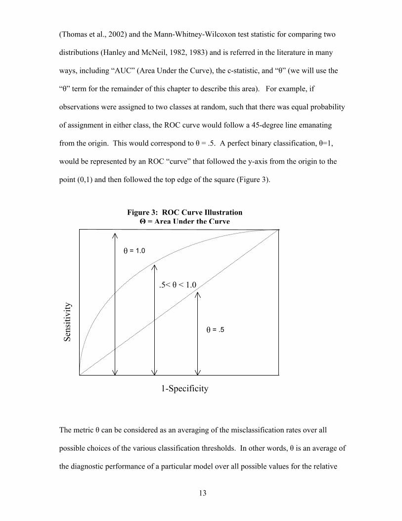
“θ” term for the remainder of this chapter to describe this area). For example, if
observations were assigned to two classes at random, such that there was equal probability
of assignment in either class, the ROC curve would follow a 45-degree line emanating
from the origin. This would correspond to θ = .5. A perfect binary classification, θ=1,
would be represented by an ROC “curve” that followed the y-axis from the origin to the
point (0,1) and then followed the top edge of the square (Figure 3).
Sens
itivi
ty
The metric θ can be
possible choices of t
the diagnostic perfor
Figure 3: ROC Curve Illustration Θ = Area Under the Curve
θ = 1.0
.5< θ < 1.0
θ = .5
1-Specificity
considered as an averaging of the misclassification rates over all
he various classification thresholds. In other words, θ is an average of
mance of a particular model over all possible values for the relative
13

misclassification severities (Hand, 2001). The interpretation of θ, where a “good” credit
risk is scored as a 1 and a “bad” credit risk is scored as a 0, is the answer to the question –
“Using this model, what is the probability that a truly “good” credit risk will be scored
higher than a “bad” credit risk”? Formulaically, θ can be represented as,
θ = ∫F(p|0)dF(p|1)dp, (2)
where F(p|0) is the distribution of the probabilities of assignment in class 0 (classification
of “bad” credit risk) and F(p|1) is the distribution of the probabilities of assignment in
class 1 (classification of “good” credit risk). The advantage of using the ROC is also its
greatest limitation – the ROC incorporates results from all possible misclassification
severities. As a result, ROC curves are highly appropriate in scenarios where no
information is available regarding misclassification costs or where the perceptions of these
costs may change based upon the evaluator. Alternatively, where some objective
information is available regarding misclassification errors, then all possible scenarios are
not relevant, making ROC curves a less appropriate evaluation method.
In this section and the previous section, we have outlined the issues and considerations
related to both model development and model evaluation. Based upon this discussion, we
will utilize empirical analysis to address our two research questions:
1. Does model development technique impact prediction accuracy?
2. How will model selection vary with the selected evaluation method?
METHODOLOGY
A real world data set was used to test the predictive accuracy of three binary classification
models, consisting of data on 14,042 applicants for car loans in the United States. The
14
data represents applications made between June 1st, 1998, and June 30th, 1999. For each
application, data on 65 variables were collected. These variables could be categorized into
two general classes – data on the individual (e.g., other revolving account balances,
whether they rent or own their residence, bankruptcies, etc) and data on the transaction
(e.g., miles on the vehicle, vehicle make, selling price, etc). A complete list of all
variables is included in Appendix A. From this dataset, 9,442 individuals were considered
to have been creditworthy applicants (i.e., “good”) and 4,600 were considered to have
been not creditworthy (i.e., “bad”), on the basis of whether or not their accounts were
charged off as of December 31st, 1999. No confidential information regarding applicants’
names, addresses, social security number, or any other data elements that would indicate
identity were used in this analysis.
An examination of each variable relative to the binary dependent variable
(creditworthiness) found that most of the relationships were non-linear. For example, the
relationship between the number of auto trades, and an account’s performance was not
linear; the ratio of “good” performing accounts to “bad” performing accounts increased
over some ranges of the variable and decreased over other ranges. This non-linearity
would have a negative impact on the classification accuracy of the two traditional
statistical models. Using a common credit industry practice, we transformed each variable,
continuous and categorical, to multiple dummy variables for each original variable.
Prior to analysis, the data was divided into a modeling file, representing 80% of the data
set and a validation file, representing 20% of the data set. The LDA and logistic analysis
models were developed using the SAS system (v.8.2).
15

There are currently no established guiding principles to assist the analyst in developing a
neural network model. Since many factors including hidden layers, hidden nodes, training
methodology can affect network performance, the best network is generally developed
through experimentation – making it somewhat more art than science (Zhang et al., 1999).
Using the basic MLP network model, the inputs into our classification networks were the
same predictor variables utilized for the LDA and logistic regression models outlined
above. Although non-linearity is not an issue with neural network models, using the
dummy variable data versus the raw data eliminated issues related to scaling (we did run
the same neural network models with the raw data, with no material improvement in
classification accuracy). Because our developed networks were binary, we required only a
single output node. The selection of the number of hidden nodes is effectively the “art” in
neural network development. Although some heuristics have been proposed as the basis
of determining the number of nodes a priori (e.g., n/2, n, n+1, 2n+1), none have been
shown to perform consistently well (Zhang et al., 1999). To see the effects of hidden
nodes on the performance of neural network models, we use 10 different levels of hidden
nodes ranging from 5 to 50, in increments of 5, allowing us to include the effects of both
small and larger networks. Backpack® v. 4.0 was used for neural network model
development.
We split our original model building file, which was used for the LDA and logistic model
development, into a separate training file and a testing file, representing 60% and 20% of
the total data file, respectively. Although the training file was slightly smaller for the
neural network modeling method relative to the LDA and logistic procedures (8,425
versus 11,233 observations), the large size of the dataset reduced the likelihood that the
16

neural network technique was competitively disadvantaged. Because neural networks
cannot guarantee a global solution, we attempted to minimize the likelihood of being
trapped in a local solution through testing the network 100 times using epochs (e.g., the
number of observations from the training set presented to the network before weights are
updated) of size 12 with 200 epochs between tests. The same validation file used for the
first two models was also applied to the validation of the neural networks.
RESULTS
The validation results for the different modeling techniques using the three model
evaluation methods are summarized in Table 1. As expected, selection of a “winning”
model is not straightforward; model selection will vary depending on the two main issues
highlighted above – the costs of misclassification errors and the problem domain.
17
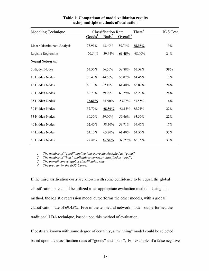
Table 1: Comparison of model validation results using multiple methods of evaluation
Modeling Technique Classification Rate Theta4 K-S Test Goods1 Bads2 Overall3 Linear Discriminant Analysis 73.91% 43.40% 59.74% 68.98% 19% Logistic Regression 70.54% 59.64% 69.45% 68.00% 24% Neural Networks: 5 Hidden Nodes 63.50% 56.50% 58.88% 63.59% 38% 10 Hidden Nodes 75.40% 44.50% 55.07% 64.46% 11% 15 Hidden Nodes 60.10% 62.10% 61.40% 65.89% 24% 20 Hidden Nodes 62.70% 59.00% 60.29% 65.27% 24% 25 Hidden Nodes 76.60% 41.90% 53.78% 63.55% 16% 30 Hidden Nodes 52.70% 68.50% 63.13% 65.74% 22% 35 Hidden Nodes 60.30% 59.00% 59.46% 63.30% 22% 40 Hidden Nodes 62.40% 58.30% 59.71% 64.47% 17% 45 Hidden Nodes 54.10% 65.20% 61.40% 64.50% 31% 50 Hidden Nodes 53.20% 68.50% 63.27% 65.15% 37%
1. The number of “good” applications correctly classified as “good”. 2. The number of “bad” applications correctly classified as “bad”. 3. The overall correct global classification rate. 4. The area under the ROC Curve.
If the misclassification costs are known with some confidence to be equal, the global
classification rate could be utilized as an appropriate evaluation method. Using this
method, the logistic regression model outperforms the other models, with a global
classification rate of 69.45%. Five of the ten neural network models outperformed the
traditional LDA technique, based upon this method of evaluation.
If costs are known with some degree of certainty, a “winning” model could be selected
based upon the classification rates of “goods” and “bads”. For example, if a false negative
18

error (i.e., classifying a true good as bad) is considered to represent a greater
misclassification cost than a false positive (i.e., classifying a true bad as good), then the
neural network with 25 hidden nodes would represent the preferred model, outperforming
both of the traditional statistical techniques. Alternatively, if a false positive error is
considered to represent a greater misclassification cost, then the neural networks with 30
or 50 hidden nodes would be selected, again, outperforming the two statistical techniques.
If the analyst is most concerned with the models’ ability to provide a separation between
the scores of good applicants and bad applicants, the K-S test is the traditional method of
model evaluation. Using this test, again, a neural network would be selected – the
network with 5 hidden nodes.
The last method of evaluation assumes the least amount of available information. The θ
measurement represents the integration of the area under the ROC curve and accounts for
all possible iterations of relative severities of misclassification errors. In the context of the
real world problem domain used to develop the eight models for this paper, prediction of
creditworthiness of applicants for auto loans, the decision makers would most likely have
some information regarding misclassification costs, and therefore θ would probably not
have represented the most appropriate model evaluation method. However, if the
available data was used, for example, as a proxy to classify potential customers for a
completely new product offering, where no pre-existing cost data was available, and the
respective misclassification costs were less understood, θ would represent a very
appropriate method of evaluation. From this data set, if θ was chosen as the method of
evaluation, the LDA model would have been selected, with a θ of 68.98. A decision
19

maker would interpret θ for the logistic model as follows – If I select a pair of good and
bad observations at random, 69% of the time, the “good” observation will have a higher
score than the “bad” observation. A comparison of the ROC curves for the three models
with the highest θ values is depicted in Figure 4.
Figure 4: ROC Curves for Selected Model Results
0.00%
20.00%
40.00%
60.00%
80.00%
100.00%
0.00% 20.00% 40.00% 60.00% 80.00% 100.00%
1-Specificity
Sens
itivi
ty
LDALogisticNN 15Random
DISCUSSION
Accurate predictive modeling represents a domain of interesting and important
applications. The ability to correctly predict the risk associated with credit applicants or
potential customers has tremendous consequences for the execution of effective CRM
strategies in the credit industry. Researchers and analysts spend a great deal of time
constructing prediction models, with the objective of minimizing the implicit and explicit
costs of misclassification errors. Given this objective, and the benefits associated with
even marginal improvements, both researchers and practioners have emphasized the
importance of modeling techniques. However, we believe that this emphasis has been
20
somewhat misplaced, or at least misallocated. Our results, and the empirical results of
others, have demonstrated that no predictive modeling technique can be considered
superior in all circumstances. As a result, at least as much attention should be allocated to
the selection of model evaluation method as is allocated to the selection of modeling
technique.
In this paper, we have explored three common evaluation methods – classification rate, the
Kolmogorov-Smirnov statistic, and the ROC curve. Each of these evaluation methods can
be used to assess model performance. However, the selection of which method to use is
contingent upon the information available regarding misclassification costs, and the
problem domain. If the misclassification costs are considered to be equal, then a straight
global classification rate can be utilized to assess the relative performance of competing
models. If the costs are unequal, but known with certainty, then a simple cost function can
be applied using the costs, the prior probabilities of assignment and the probabilities of
misclassification. Using a similar logic, the K-S test can be used to evaluate models based
upon the separation of each class’s respective distribution function – in the context of
predicting customer risk, the percentage of “good” applicants is maximized while the
percentage of “bad” applicants is minimized, with no allowance for relative costs. Where
no information is available, the ROC curve and the θ measurement represent the most
appropriate evaluation method. Because this last method incorporates all possible
iterations of misclassification error severities, many irrelevant ranges will be included in
the calculation.
Adams and Hand (1999) have developed an alternative evaluation method, which may
address some of the issues outlined above, and provide researchers with another option for
21

predictive model evaluation – the LC (loss comparison) index. Specifically, the LC index
assumes only knowledge of the relative severities of the two costs. Using this simple, but
realistic estimation, the LC index can be used to generate a value which aids the decision
maker in determining the model which performs best within the established relevant range.
However, the LC Index has had little empirical application or dedicated research attention
to date. It represents an opportunity for further research, refinement and testing.
Clearly no model evaluation method represents a panacea for researchers, analysts or
decision-makers. As a result, an understanding of the context of the data and the problem
domain is critical for selection, not just of a modeling technique, but also of a model
evaluation method.
22

APPENDIX A: Listing of original variables in data set
Variable Name Variable Label
1. ACCTNO Account Number 2. AGEOTD Age of Oldest Trade 3. BKRETL S&V Book Retail Value 4. BRBAL1 # of Open Bank Rev.Trades with Balances>$1000 5. CSORAT Ratio of Currently Satisfactory Trades:Open Trades 6. HST03X # of Trades Never 90DPD+ 7. HST79X # of Trades Ever Rated Bad Debt 8. MODLYR Vehicle Model Year 9. OREVTR # of Open Revolving Trades 10. ORVTB0 # of Open Revolving Trades With Balance >$0 11. REHSAT # of Retail Trades Ever Rated Satisfactory 12. RVTRDS # of Revolving Trades 13. T2924X # of Trades Rated 30 DPD+ in the Last 24 Months 14. T3924X # of Trades Rated 60 DPD+ in the Last 24 Months 15. T4924X # of Trades Rated 90 DPD+ in the Last 24 Months 16. TIME29 Months Since Most Recent 30 DPD+ Rating 17. TIME39 Months Since Most Recent 60 DPD+ Rating 18. TIME49 Months Since Most Recent 90 DPD+ Rating 19. TROP24 # of Trades Opened in the Last 24 Months 20. CURR2X # of Trades Currently Rated 30 DPD 21. CURR3X # of Trades Currently Rated 60 DPD 22. CURRSAT # of Trades Currently Rated Satisfactory 23. GOOD Performance of Account 24. HIST2X # of Trades Ever Rated 30 DPD 25. HIST3X # of Trades Ever Rated 60 DPD 26. HIST4X # of Trades Ever Rated 90 DPD 27. HSATRT Ratio of Satisfactory Trades to Total Trades 28. HST03X # of Trades Never 90 DPD+ 29. HST79X # of Trades Ever Rated Bad Debt 30. HSTSAT # of Trades Ever Rated Satisfactory 31. MILEAG Vehicle Mileage 32. OREVTR # of Open Revolving Trades 33. ORVTB0 # of Open Revolving Trades With Balance >$0 34. PDAMNT Amount Currently Past Due 35. RVOLDT Age of Oldest Revolving Trade 36. STRT24 Sat. Trades:Total Trades in the Last 24 Months 37. TIME29 Months Since Most Recent 30 DPD+ Rating 38. TIME39 Months Since Most Recent 60 DPD+ Rating 39. TOTBAL Total Balances 40. TRADES # of Trades 41. AGEAVG Average Age of Trades 42. AGENTD Age of Newest Trade 43. AGEOTD Age of Oldest Trade 44. AUHS2X # of Auto Trades Ever Rated 30 DPD
23

45. AUHS3X # of Auto Trades Ever Rated 60 DPD 46. AUHS4X # of Auto Trades Ever Rated 90 DPD 47. AUHS8X # of Auto Trades Ever Repoed 48. AUHSAT # of Auto Trades Ever Satisfactory 49. AUOP12 # of Auto Trades Opened in the Last 12 Months 50. AUSTRT Sat. Auto Trades:Total Auto Trades 51. AUTRDS # of Auto Trades 52. AUUTIL Ratio of Balance to HC for All Open Auto Trades 53. BRAMTP Amt. Currently Past Due for Revolving Auto Trades 54. BRHS2X # of Bank Revolving Trades Ever 30 DPD 55. BRHS3X # of Bank Revolving Trades Ever 60 DPD 56. BRHS4X # of Bank Revolving Trades Ever 90 DPD 57. BRHS5X # of Bank Revolving Trades Ever 120+ DPD 58. BRNEWT Age of Newest Bank Revolving Trade 59. BROLDT Age of Oldest Bank Revolving Trade 60. BROPEN # of Open Bank Revolving Trades 61. BRTRDS # of Bank Revolving Trades 62. BRWRST Worst Current Bank Revolving Trade Rating 63. CFTRDS # of Financial Trades 64. CUR49X # of Trades Currently Rated 90 DPD+ 65. CURBAD # of Trades Currently Rated Bad Debt
24

ENDNOTES 1 Federal Reserve System Report (2003). http://www.federalreserve.gov/rnd.htm
25

REFERENCES
Adams, N. M. and Hand, D.J. (1999). Comparing classifiers when the misclassification costs are uncertain. Pattern Recognition, 32, 1139-1147. Atiya, A. F. (2001). Bankruptcy prediction for credit risk using neural networks: A survey and new results. IEEE Transactions On Neural Networks, 12 (4), 929-935. Berardi, V. L. and Zhang, G. P. (1999). The effect of misclassification costs on neural network classifiers. Decision Sciences, 30 (3), 659-682. Fisher, R. A. (1936). The use of multiple measurement in taxonomic problems. Ann. Eugenics, 7, 179-188. Gim, G. (1995). Hybrid Systems for Robustness and Perspicuity: Symbolic Rule Induction Combined with a Neural Net or a Statistical Model. Unpublished Dissertation. Georgia State University, Atlanta, GA. Hand, D.J. (2002). Good practices in retail credit scorecard assessment. Working Paper. Hand, D. J. (2001). Measuring diagnostic accuracy of statistical prediction rules. Statistica Neerlandica, 55 (1), 3-16. Hanley, J.A. and McNeil, B.J. (1983). A method of comparing the areas under a Receiver Operating Characteristics curve. Radiology, 148, 839-843. Hanley, J.A. and McNeil, B.J. (1982). The meaning and use of the area under a Receiver Operating Characteristics curve. Radiology, 143, 29-36. Kimball, R. (1996). Dealing with dirty data. DBMS Magazine, 9 (10). http://www.dbmsmag.com/9609d14.html Reichert, A. K., Cho, C. C., and Wagner, G.M. (1983). An examination of the conceptual issues involved in developing credit scoring models. Journal of Business and Economic Statistics, 1, 101-114. Richeson, L., Zimmerman, R., and Barnett, K. (1994). Predicting consumer credit performance: Can neural networks outperform traditional statistical methods? International Journal of Applied Expert Systems, 2, 116-130. Swets, J.A., Dawes, R.M., and Monahan, J. (2000). Better decisions through science. Scientific American, 283 (4), 82-88. Taylor, P.C. , and Hand, D.J. (1999). Finding superclassifications with acceptable misclassification rates. Journal of Applied Statistics, 26, 579-590. Thomas, L.C., Edelman, D.B., and Cook, J.N. (2002). Credit Scoring and Its Applications. Philadelphia: Society for Industrial and Applied Mathematics. Vellido, A., Lisboa, P.J. G., and Vaughan, J. (1999). Neural networks in business: a survey of applications (1992-1998). Expert Systems with Applications, 17, 51-70.
26

West, D. (2000). Neural network credit scoring models. Computers and Operations Research, 27, 1131-1152. Zhang, G., Hu, M.Y., Patuwo, B.E., and Indro, D.C. (1999). Artificial neural networks in bankruptcy prediction: General framework and cross-validation analysis. European Journal of Operational Research, 116, 16-32.
27

28