assessment of distance measurement using a 3- …

ASSESSMENT OF DISTANCE

MEASUREMENT USING A 3-

AXIS DIGITAL ACCELEROMETER

Guillermo Puchalt Casáns Miguel Alcañiz Fillol, Rafael Masot

Master's Degree in Sensors for Industrial Applications

School of Design Engineering

1

Contents

Abstract ......................................................................................................................................... 1 1. State of the Art ...................................................................................................................... 2 2. Materials and Methods ......................................................................................................... 5

2.1. Design of the pedometer .............................................................................................. 5 2.1.1. Aspects to be considered ...................................................................................... 5 2.1.2. Block Diagram of Device ........................................................................................ 6 2.1.3. Design of hardware ............................................................................................... 6 2.1.4. Design of firmware .............................................................................................. 11 2.1.5. Design of software .............................................................................................. 16

2.2. Design of the processing algorithms ........................................................................... 17 2.2.1. Aspects to be considered .................................................................................... 19 2.2.2. Integrate all the data approach ........................................................................... 19 2.2.3. Integrate the data in batches approach .............................................................. 21 2.2.4. Integrate the data in steps approach .................................................................. 21

2.3. Design of the experimental setup ............................................................................... 25 2.3.1. Other pedometers used for comparison............................................................. 25 2.3.2. Protocol Followed ............................................................................................... 25

3. Results and Discussion ........................................................................................................ 30 3.1. Aspects to be considered ............................................................................................ 30 3.2. Observations of integrating all the data (R2=0,9710) .................................................. 30 3.3. Observations of integrating the data in batches (R2=0,8513) ..................................... 34 3.4. Observations of integrating the data based on the steps (R2=0,9835 (XYZ) and R2=0,9791 (XZ)) ........................................................................................................................ 34 3.5. Comparison ................................................................................................................. 36

4. Conclusions and Improvements .......................................................................................... 37 5. Bibliography ........................................................................................................................ 38 Annex 1: PIC Firmware implemented ......................................................................................... 40 Annex 2: Commands used between Microcontroller – PC ......................................................... 55 Annex 3: Device schematic.......................................................................................................... 57 Annex 4: Description of the Computer Interface ........................................................................ 58

Assessment of distance measurement using a 3-axis digital accelerometer

1

Abstract

This project consisted on evaluating the capability of a triaxial accelerometer as a straight

forward distance measuring pedometer as the current existing ones rely on a user calculated

mean stride for multiplication with the step count. A device was developed for the purpose using

the ADXL345 triaxial accelerometer and the PIC18LF14K22 microcontroller in combination with

MATLAB for data filtering and processing. Three approaches were taken in consideration when

calculating the distance walked by the subject through double integration of the acceleration

(integrating all the data (R2=0,9710), integrating the data in batches (R2=0,8513), integrating the

steps (R2=0,9835) and integrating the steps (only XZ axes) (R2=0,9791)) and results were

contrasted against a mechanical pedometer (R2=0,9947), a smartphone app pedometer

(R2=0,0266) and the real distance walked. From this project it was known that using an

accelerometer and any of the three approaches a distance of at least five meters could be

measured with a coefficient of variation of 4,2278%, although the first approach proved to be

very reliable for distances of twenty meters (Cv=2,5622%).

Keywords: accelerometer, distance, pedometer, double integration


2

1. State of the Art

A pedometer is a device used to measure daily activity in the form of a step count.

Nowadays pedometers offer other functions, like calorie counter, time exercising, mean speed

and above all, distance traveled. But there is a catch to this function, and is that it does not

measure the truly distance traveled, but it counts the number of steps the user has done and

multiplies it by a mean value of the user’s stride. This method is not reliable for knowing the true

distance the user has traveled because the stride’s length can vary for various reasons:

a) If the user walks at a slow speed, or has a considerably body mass, the steps will not be

counted, consequently, less distance [1].

b) If the user performs longer, or shorter, strides for any particular reason1, the total

distance traveled will be different than the real one is.

c) Any movement done by the body besides walking could increase the step count,

therefore, greater distance will be displayed.

d) If the user has a peculiar gait, the step count will not be consistent, hence the distance

traveled will be different than the real one.

But besides those general problems, there are also some special problems depending on the

type of technology used by the pedometer. On the market there are three types of technology

regarding pedometers [2]:

1) Based on a mechanical system (Figure 1, pg 4)

This type of technology is the cheapest of all three but comes with its own

drawbacks. It is composed of a pendulum that moves vertically up and down when a

step is done, and such movement activates a switch, increasing the step count. Because

of this type of behavior, the pedometer brings some problems, besides those already

mentioned:

a) It must be perpendicular to one of the legs, otherwise it will not count the

steps accordingly. This happens because the pendulum moves due to hip

movement as a consequence of setting the foot down. If the pedometer is

not in line with the movement propagation up the leg, the pendulum will

not work.

b) Every step has to be uniform as any abnormal movement of the legs will not

move appropriately the pendulum and miscount the step, or count more

than once.

c) The return spring that stabilizes the pendulum can wear off over time and

make the pedometer more sensitive to slightly active movements. Although

this is one of the reasons usually found, according to [3], after intensive use

the pedometer will have an error less than 5% in relation with the amount

of steps counted.

1 Like walking up, or down, a hill or stairs


3

d) Because the pendulum relies on the vertical propagation of the step

movement, if the user is walking up, or down, a hill the pendulum will not

move appropriately either.

2) Based on an acceleration sensor

This type of technology is the most reliable on the market as it detects the

acceleration caused by the movement propagation of the step. Because of its multiple

axes, positioning of the pedometer in the body is not as crucial as the previous type of

technology. Yet, it still has its problems, like those described in general terms

beforehand.

Although the device developed also relies on an accelerometer it differs from

the pedometers using this type of technology that it provides the distance measurement

directly rather than being calculated from the amount of steps.

3) Based on a GPS receiver

This type of technology is the most expensive of all, but can give really good

results. Of course, it will work only if the user is physically moving in space and it receives

a strong GPS signal. Therefore, when walking on a treadmill, or being indoors, or being

in a location with no GPS signal reception, the pedometer will not measure the distance

traveled accurately.

The objective of this project is to create a low-cost pedometer that measures the distance

traveled, indoors or outdoors, with the aid of acceleration measurements, without knowing

the amount of steps or the mean stride length or relying on other types of position data2. This

way, the true distance traveled will be measured accordingly and independently of the speed of

the user, its stride variation, its gait, where it goes and what it does.

Of course, walking in a treadmill will not be possible either as the device will physically be in

the same region of space rather than moving forward.

2 Based on [16], gyroscope data can be left aside because during gait the rotational components can be redefined as a function of translational components of acceleration (if it was necessary to now the rotational components) because such components are large enough to be detected. If, like in aerospace navigation, the rotational components were small then they could not be a function of translational components as they will be too small to be detected.


4

Figure 1: Insides of a pedometer with a mechanical system

Pendulum

Hair – Spring Electric Contact


5

2. Materials and Methods

2.1. Design of the pedometer

2.1.1. Aspects to be considered

From the read literature, two key features of the device’s characteristics were established. These features were:

Sampling frequency of 100 Hz or higher

Despite that the data will be filtered through a low pass filter at approximately 20 Hz, sampling was carried at 100 Hz. In most of the literature the sampling frequency was between 60 Hz and 500 Hz, being 100 Hz the most used sampling frequency.

Acceleration range of ±2g

Based on the conclusions from [4], the acceleration sensor should have a range of ±6g. Reviewing the article in depth it was found that when walking the acceleration amplitudes at the pelvis were of [-0.3 0.8]g in the vertical axis and ±0.2g in the horizontal axis while walking. Based on this data, a range of ±2g was selected as the sensor used does not allow for anything smaller.

Each data package that represented one sample of the acceleration profile had the following structure of 8 bytes:

1) Start byte 2) 6 bytes of data (in pairs of 2 bytes per axis as the data is of 10 bits of length) 3) Checksum

At lab the available wireless circuits were not sufficient for transmitting in real time the

amount of data produced every second and store it in file at the computer3. To solve this issue, instead of transmitting the data wirelessly, it was stored in a memory chip and later downloaded to the computer with the help of an UART – USB converter cable.

3 Although the wireless circuit used was capable of a baud rate of 9600 bps (the circuit generated 6400 bits per second), experimentation showed that the computer was not capable of receiving such amount of data.


6

2.1.2. Block Diagram of Device

2.1.3. Design of hardware

The device circuit was developed using Proteus 8 Design Suite software, transferred to a two side PCB (Figure 2, pg 7) through photoengraving, and applied chemical etching. Consideration was taken for the battery pack placement and fixing4, as well as the sensor fixing to the PCB5. The latter is a crucial aspect of the device because if the sensor was badly fixed to the circuit board, it will resonate while the subject walks and it will record its own acceleration oscillations6.

Due to the communication problem discussed earlier7 a memory chip had to be chosen for

data collection. By recommendation of the directors, it was used a SPI flash memory chip, but several requirements had to be fulfilled:

A) Memory capacity

The amount of memory required for the gathering of data was

calculated based on a 5-minute time span of data gathering and the amount of data generated per second in bits:

(3 axes x 2 byte/axis + start byte + checksum byte) x 100 samples/s = 800 bytes/s 800 bytes/s x 5 min x 60 s/min = 240 kB 240 kB x 8 bits/byte = 1.92 Mb

So the memory’s capacity had to be equal or greater than 1.92 Mb.

4 The battery pack was placed in the bottom layer and caution was taken that all of the electronic components were placed facing up in the top layer so that they do not overlap. 5 The holes used for fixing had to be placed somewhere where they had minimal impact to the paths. This could not be done for the battery fixing holes as it was fixed in the middle as described earlier. 6 Mechanical Considerations for mounting, pg 28 [5] 7 Aspects to be considered (pg 4)


7

Holes for the sensor fixing

Holes for the sensor fixing

Figure 2: PCB representation with all the components and board dimensions


8

B) Sequential writing function8

This function is crucial for the device’s operation as it allows for faster writing procedures of data in the memory chip in comparison with singly byte writing procedures.

C) Erase all memory command

Of the memory chips searched, some didn’t have this command available. Instead, the memory chip had to be erased with multiple executions of the erase command9. For simplification of the firmware design it was preferably that the memory chip had this function available.

D) Availability in Proteus 8 Design Suite

Although it is not an essential feature to be fulfilled, it will simplify much the debugging process of the firmware design using Proteus 8 Design Suite. Additionally, if the memory chip is already in the program’s library it will also have its packaging.

E) Had to be available at Farnell Components preferably

This feature was more of a recommendation from the directors as they were

already about to make a purchase of materials for the department from this provider.

Using the electronic components search engine Octopart10 and looking over the datasheets

of the obtained results, the 2Mb flash memory chip SST25PF020B (Figure 4, pg 9) was the best candidate. It met all of the requirements except for one: It was not available in the Proteus 8 Design suite program.

This inconvenience for the hardware design was solved by using a random chip that shared the same package (SOIC-8) and reassigning the pinout numbers in the same way that the original memory chip has. In the case of the firmware design process, the problem was solved by substituting the flash memory chip for an SRAM memory chip (23A256) that was available in the Proteus 8 libraries.

The behavior between both memory chips is similar regarding for the reading and writing data sequences. The only important difference between both of them came on the way they handled the sequential writing instruction sequences. While the SRAM memory only required at the beginning of the sequence the sequential write command, the Flash memory required at the beginning the sequential write command and the 3-byte address, and for every two desired bytes to be written, the sequential write command had to be sent beforehand again.

One final aspect to comment about the flash memory chip is that during testing it was found out that a decoupling capacitor of 0.1 µF was required for filtering noise from its power supply pin (Vdd) for proper operation or it wouldn’t work at all.

The accelerometer used in the device was the ADXL345, which is a widely used MEMS

accelerometer. It is integrated in a PCB (Figure 5, pg 10) alongside with a compass, a gyroscope, a barometer and a thermometer. The most frequent use of this type of sensors is for inertial

8 This function allows writing several bytes continuously without having to write every time the address to store each byte. 9 Depending on the memory chip, it could be erased by sector of memory of different sizes but nor the entire memory available. 10 https://octopart.com


9

Figure 4: Breakoutboard with a similar memory chip used (the difference relies on the operational temperature range).

Nº Board Component

1 Accelerometer

2 Mechanical fixing of multi-sensor board to PCB

3 Power supply and selection jumper

4 Mechanical fixing of battery pack

5 Decoupling capacitor

6 Microcontroller

7 UART communication port

8 Status LEDs

9 Memory chip

10 Firmware download port

11 Mode selection push button

12 Battery pack (2xAA)

Figure 3: Final product of device with component indication

1

3

5

4

6

2

10

11

7

12

8

9


10

Compass Gyroscope

Accelerometer Pressure and Temperature Sensor

Pins used

Figure 5: GY-80 PCB sensor platform used


11

measuring equipment for airplane navigation, medical equipment, gaming and pointing devices, industrial instrumentation and hard disk drive protection [5].

This accelerometer presented the same problem as the flash memory chip with Proteus 8 Design Suite. It was substituted for debugging purposes by the I2C controlled ADC converter (MCP3424). Three signals were attached to simulate acceleration measurements. Little difference was found between both of them besides the commands used for communication. Meanwhile, its package footprint did not present a challenge as it was already integrated in a PCB and had a 0.1” SIL pinout for interfacing with the device.

The microcontroller used in this project was the PIC18LF14K22 8-bit microcontroller

which is ideal for this master’s degree final project, due to its capacity, cost and flexibility. Additionally, it was used in different subjects of the Master, so the available tools to work with it were already available. It was operated with a clock frequency of 16 MHz11.

During design it was evaluated if the device will be powered by a 3xAA (4,5V) or 2xAA (3V) battery pack. The difference between using each one of them relied on whether using a 3,3V low-dropout linear voltage regulator or not. Because all of the components used could work at 3V or lower it was decided that with a 2xAA battery pack will be sufficient for the power needs of the device. Just in case, it was added the possibility of allowing the device being powered by an external power source so that the batteries were not consumed while debugging.

Furthermore, during the hardware designing stage, it was considered that it was needed three LEDs for debugging purposes that will act as indicators of mode in which the device is working (Figure 3, pg 9).

2.1.4. Design of firmware

For the design of the microcontroller firmware, it was used MPLAB X IDE and C

programming language, aided with the Proteus 8 Design Suite software for basic debugging

(Figure 6, pg 12) . As mentioned previously, some hardware components were not available in

Proteus 8 Design Suite and were substituted by components that had certain resemblance with

the originals12. Of course, once the final hardware was created, the debugged firmware had to

be changed to adapt to such hardware and debug again although much less thoroughly.

Besides the debugging adaptation problem, there was a communication problem. As

mentioned previously, it was used SPI and I2C communication simultaneously because the

acceleration sensor cannot communicate through SPI13. So, in order to overcome this problem,

an improvised software based SPI communication system was developed using four GPIO pins

as the clock, input, output and CE̅̅̅̅ pins. The SPI communication sequence worked as follows:

1) CE̅̅̅̅ pin set to zero

2) SCL pin set to cero

3) MOSI pin set to the result of applying an AND mask with the number 0x80 and

shifting to the left seven times

11 It was the fastest clock speed that the internal oscillator of the microcontroller could achieve. This was the amount of time of capturing the acceleration data and storing it in the memory chip was reduced to the minimum amount of time. 12 Design of hardware, pg 5 13 Technically speaking, it can communicate through SPI, but the PCB sensor board had the connections made for I2C communication and they couldn’t be modified.


12

Figure 6: Diagram of how the device is used during the data capture procedure described in pg 25, Protocol Followed (in red at firmware level and in blue at procedure level)


13

4) Input data variable is rewritten with the original variable shifted to the right once.

5) SCL pin is set to one

6) Output data variable is set to be the result of adding the logical value of the MISO

pin and the result of shifting once the output data variable

7) Repeat steps 1-5 another seven times

8) If the RW variable is one (indicating that the function was called for a reading

purpose), return the output data variable.

9) CE̅̅̅̅ pin is set to one

I2C communication was performed using the PIC18F14K22 MSSP peripheral and the I2C

library available.

A function was implemented that combined the software based SPI communication and

the I2C communication systems14. That way, the firmware was simplified as it was required many

times to use one of the communication systems.

When the device is powered up, all the required peripherals15 of the microcontroller are

configured, as well as the memory chip16 and the sensor17, and the microcontroller is set for the

one of its operational modes.

There are 5 different operational modes that run their functions once the external

interrupt is activated by the device’s button. In order to avoid multiple external interrupts

because of the bouncing of the signal of the button, Timer3 was used as a debouncing

mechanism. By using the timer, two conditions (timer and external interrupt activation) had to

be achieved in order to change mode with the button.

These modes are:

a) Standby prior offset calculation (Green LED off, Red LED on, Orange LED on)

This mode is responsible for erasing the memory chip completely so that the

new data does not get mixed with old data. When the device powers up, it starts on

this mode but doesn’t execute its functions as the interrupt handler hasn’t been

called.

b) Offset calculation (Green LED off, Red LED off, Orange LED blinking)

This mode is responsible of calculating the offset of each axis. Once the offset is

calculated, this mode will not allow any recalculation of the offset until the device

µC is powered down18.

14 pg 13 for further details 15 Timer0, Timer1, Timer3, USART, MSSP (for I2C communication for the acceleration sensor), Internal oscillator, Interrupts configuration and GPIO configuration for the software based SPI system, LEDs, and button. 16 Disabling overwrite protection 17 Full resolution mode, right data justification, ±2g range (register 0x31 pg 26 [5]), Stream FIFO mode (register 0x32 pg 27 [5]) and setting the output data rate at 200 Hz (register 0x2C pg 25 [5]) 18 A reset command will also work


14

There is a 10 second delay (with Timer1) prior to executing this function. That

way, if the user doesn’t want to execute an offset calculation process it can press

again the button before the time is up.

Once the delay has elapsed, the device turns on the sensor, resets the offset

variables inside the microcontroller, and captures n samples19 of data at a rate of

100 Hz20. Once the samples were collected, a mean value was calculated for each

axis, divided by the sensitivity of the sensor and multiplied by -120. Because the Z

axis is in an upright position, the offset calculated will have registered the value of

gravity as well. This value was subtracted from the mean value calculated, assuming

perfect sensitivity. As mentioned in the sensor’s datasheet, sensitivity can vary for

different reasons and by so, the Z axis offset result can be different than what should

actually be. Based on the example given in the sensor’s datasheet this aspect can be

discarded as the error due to sensitivity differences is minimal.

c) Standby for capture of data (Green LED off, Red LED on, Orange LED off)

This mode holds the device on standby previous to the capture mode while the

device is set in its final position on the subject. This mode is crucial as offset

calculation is done on a flat surface rather than on the subject.

d) Capture of data (Green LED blinking, Red LED off, Orange LED blinking)

In this mode, the device captures the data relative to the acceleration profile

that the acceleration sensor detects. Before capturing data, the memory chip is

prepared for the sequential writing processes and the sensor is turned on. Once the

preparations are completed, Timer0 is enabled and the capturing process begins.

For every time the Timer0 interrupt activates, the interrupt handler does the

following:

1) Reload of Timer0 registers based on the selected sampling frequency. Turn

the orange LED on and toggle the green LED.

2) Assign the starting value to the checksum byte of the data package.

3) Read the data from the registers that correspond to the axis of interest with

the help of the communication function. Because the function returns the

value as a 16-bit integer, the number has to be fragmented in 2 8-bit

integers. Each individual number is set in its corresponding position in the

data package21.

4) Add to the checksum byte of the data package the two new bytes.

5) Repeats steps 2-4 for the two other axes.

6) Add one to the data package counter variable.

7) Send the data package to the memory chip.

8) Turn off the orange LED.

19 The amount of samples to be taken is specified by the constant samples 20 Following the recommendations given by the sensor’s datasheet ( [5] pg 30) 21 The data package sent to the memory chip has 8 bytes has this structure: Start byte – X axis 2nd byte – X axis 1st byte – Y axis 2nd byte – Y axis 1st byte – Z axis 2nd byte – Z axis 1st byte – Checksum


15

The LED control is important during the capture mode as indicates that the

capture process is happening (green LED) and allows to measure with an

oscilloscope the duration of the capturing process (orange LED). This is proven

useful when debugging the firmware in order to evaluate if the firmware fulfills the

timing requirements of the sampling frequencies22.

e) Computer communication (Green LED on, Read LED on, Orange LED blinking)23

In this mode the device is under the control of the computer interface. It is used

mainly for transferring the acceleration data to the computer, but it is also used for

debugging purposes (selecting a different sampling frequency, controlling the

memory chip or the sensor, microcontroller reset, etc). Additionally, this mode

disables any chance of writing in the memory chip by accident as well as turn off the

sensor.

Data packages sent and received from the computer interface vary in length. In

the case of data packages received from the PC, this were always 5 bytes long24

whereas the data packages received from the device varied from 3 to 10 bytes,

depending on the data transmitted.

Last but not least, the entire process of capturing and storing data in the memory chip

had to be fast enough in order to accomplish the desired sampling frequencies. To achieve this

goal, two sections of the firmware went through trial and error experimentation to test the time

it took to capture and store data. This amount of time was measured by using the oscilloscope

and testing when the orange led turned on and off. Such sections were:

A) The Timer0 interrupt handler

The interrupt handler had to be as simple as possible. One feature that

is seen in the code is that the checksum function is not used although it

existed. From experimentation it was observed that calculating the

checksum manually made the handler faster.

Additionally, the sequential write process was helpful with this task, as

it only required 3-byte packages consisting of the sequential-write

command and two of the 8 bytes of each data package. The initialization of

such process was carried when the capture mode was selected.

B) The communication function

The communication function proved to be a challenge among all the

programming as it was called up to 15 times per data capture (3 times for

reading data of each axis, and 4 times for every data package sent to the

memory chip). It had to be fast enough so that the sampling frequency

timing requirements could be achieved.

22 See pg 5 for further explanation. 23 See Annex 2: Commands used between Microcontroller – PC for details on the commands used 24 The structure of the data package was: Start Byte – Command Byte – Data component nº1 – Data component nº2 - Checksum


16

On the first versions of the firmware, the way to differentiate between

SPI and I2C communication was with the who variable and detecting it if was

positive (representing the I2C addresses) or negative (SPI communication).

From experimentation it was observed that if instead of detecting a negative

value, it was detected a positive value (one higher than the highest I2C

address value), the communication function worked much faster. Also, the

reset of the output variable of the I2C communication part was done only

when such communication was required, hence saving more time.

One aspect of the I2C communication that affected the design of the

function was that two bytes could be read from the sensor. So rather than

setting the output of the function as an unsigned char, it was set as an

integer, so that two bytes of data could be passed out and later the firmware

process the data and separates the number in two independent bytes.

2.1.5. Design of software

The computer interface that will access and control the device was implemented with GUIDE

in MATLAB R2012b. It was designed for basic communication with the device as well as for data

retrieval. Data processing is done through separate scripts as described in the next chapter.

The interface has four buttons at the left side that take care of data recovery, manual

memory erase and sending specific commands. Such commands can be chosen from the drop

down list of pre-established commands but can only be sent if the manual control mode is

enabled in the interface. There are two text boxes for establishing addresses and data to be sent

through the I2C/SPI buses. These text boxes are enabled only when the selected command

requires of such information.

There is another dropdown list for selecting the PC communication port that is connected

to the device25.

Communication from the device to the computer had certain complications as the received

data packages were sometimes incomplete. A command26 was programmed in the firmware so

that in case of such problem it will ask the microcontroller to transmit again the last data package

sent.

All of the received data packages that were related to the device operation contained the

relevant information between the start byte and the checksum and are displayed directly in the

interface. Meanwhile, the data packages that carry the measured acceleration have a different

structure27. This way it is checked if data had been lost during the transfer.

Because the acceleration data is a 10-bit long number per axis, each piece of data has 6

bytes/sample28, and when received at the computer they are converted into three digital

25 In case the computer has multiple available communication ports. 26 Annex 2: Commands used between Microcontroller – PC, command 19. 27 Start byte – 2nd byte of data package number – 1st byte of data package number – Data bytes – Checksum 28 Where each two bytes represent an acceleration value in one axis.


17

numbers with the help of function. This function combines each pair of bytes into one number

and because the numbers are in two’s complement, they are converted to regular numbers first.

Once all three numbers are converted from their bytes, they are written into a text file and saved

at the established destination29. The number was not converted into international units in the

data retrieval process because the sensitivity value could be changed between experiments.

They were converted at the processing scripts.

2.2. Design of the processing algorithms

Development of the different processing algorithms was done using MATLAB software once

the data was captured. All of the scripts written had a basic structure:30

1) All of the repetitions of the acceleration data set files are read and converted into

international units (m/s2).

2) Each repetition has its own structured variable associated, where any processing of the

repetition is stored. Because the sensor recorded the moments in which the device’s

button is pressed, the scripts cuts away the first 5 seconds of data and the last 1531.

3) Absolute acceleration values are calculated in case of being needed, as well the gravity

value measured, the time vector, the frequency vector and its name32.

4) Double filtering processing of each repetition of the data set.

5) Data processing.

6) At the end of the script, a table is created showing calculated distance walked, standard

deviation, 1st harmonic, number of steps and time taken to walk the distance33.

Consideration was taken on if data of all three axes had to be used or not. Based on [6], the

reference plane parallel to the ground will be recording the foot down and heel up event

acceleration responses. Such data doesn’t represent at all the inertial movement of the body

and excluding it could make the data processing much easier.

But because the reference planes are tilted, the acceleration component due to body

movement is distributed along all the axes and hence elimination of one of them will omit part

of valuable data. Still, an attempt was carried in one of the algorithms to process the data by

removing the data of the axis that represented the most of such unwanted acceleration data,

whereas in the other algorithms the absolute magnitude of acceleration was used.

Within each algorithm there is a pseudo-algorithm responsible for counting steps. This

pseudo-algorithm is independent of the data processing algorithms but it does use both filtering

29 In this Project, the files were named following a specific structure: Distance walked – Repetition number – Location in the body – if it had offset 30 Following more or less the guidelines established at [14] 31 Further explained on 2.3.2 Protocol Followed pg 18 32 Except for the frequency vector, each aspect of each repetition of the acceleration data set is slightly different to the others. That is why the time vectors and gravity values were calculated for each repetition. 33 All other numerical values of interest were displayed through the command window in MATLAB.


18

Figure 7: First data set for 30m distance


19

stages. It was used for comparison of the data from the device with the data obtained from the

other pedometers34.

2.2.1. Aspects to be considered

Although most of the development were based on the different approaches, the filtering

portion of the algorithms was based partially on the literature used. For instance, on most of the

literature, part of the filtering process consisted on applying a low pass filter with a cut-off

frequency below the 20 Hz mark so that unwanted noise got eliminated.

In some cases [7], it was recommended to apply a high pass filter at very low frequencies

(<2 Hz) so that the gravity component of the data could be attenuated as much as possible.

Although this turned up to be true, it did produce an unwanted response on the data in the form

of ringing. This is believed to happen because any offset in the data due to the gravity

component was interpreted as a step function and filtering of such signal caused such response.

The way this problem was solved was subtracting this offset due to the gravity component,

rather than filtering it out35. Of course, such component was calculated from the data itself as

the acceleration sensor can’t make an exact measure of gravity and subtracting its theoretical

value will still bring the same problem again.

This bandpass filtering is considered the first stage of filtering process of every data set. The second stage of filtering consists of a low-pass filter with a cut-off frequency at the first harmonic36 of the acceleration data. This harmonic is believed to correspond to the subject’s speed in terms of steps/s so any data at higher frequencies is just a harmonic multiple or acceleration due to other forces. But from trial and error it was observed that a cut-off frequency at the first harmonic was too strong, so the cut-off frequency was changed to the second harmonic of the data set.

The frequency value of the second harmonic was not obtained through FFT analysis as it had been done with the first harmonic, but rather calculated as a multiple of the first harmonic. This was done as so because the harmonic detection procedure based itself on search for peaks of power in the FFT analysis results and it was not always found the second harmonic as the true second harmonic. What happened was that in some occasions the true second harmonic peak had less power in comparison with other harmonic power peaks.

Testing also showed that using higher harmonics only added noise to the data set and increased variance in the final results.

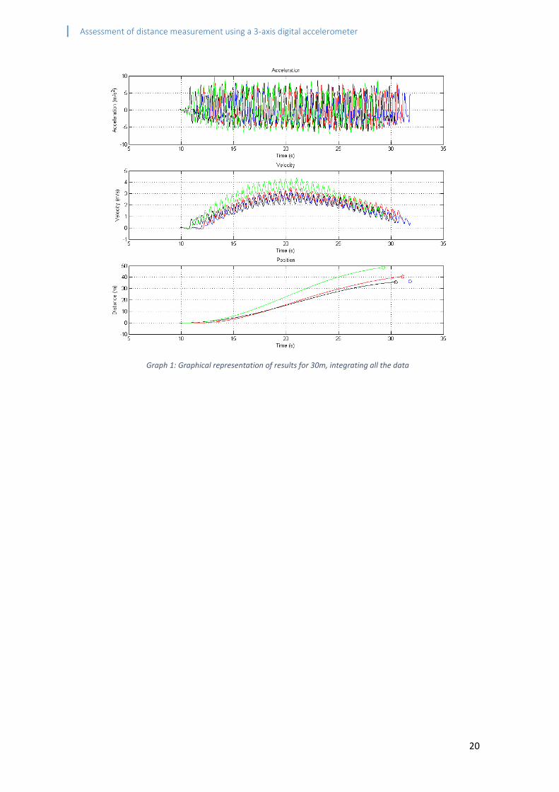
2.2.2. Integrate all the data approach

This approach is the simplest of all the ones tried. Basically it integrates all of the acceleration data after applying both filtering stages to obtain the speed of the subject, and it is integrated again to obtain the distance traveled. See Graph 1 (pg 20) for an example.

.

34 Other pedometers used for comparison (pg 18) 35 A similar method was used on [12], as one of the algorithms studied in such work was similar to the basic ideas (filtering, absolute magnitude of acceleration and gravity subtraction) used in the tested algorithms of this project 36 Found through FFT analysis of each data set.


20

Graph 1: Graphical representation of results for 30m, integrating all the data


21

2.2.3. Integrate the data in batches approach

In this approach, the valid acceleration data set was first filtered and then cut in portions of approximately five seconds in length. Each data portion was subsequently integrated twice. When integrating speed, it was taken into consideration the final value of the previous data portion integration as the initial value for the next data portion integration. The same was done when integrating the speed results into distance. See Graph 2 (pg 22) for an example.

2.2.4. Integrate the data in steps approach

This approach is similar to the previous one but rather than slicing in sections of time, each portion is limited by each step the subject performs. This way each step is considered as independent from the rest. According to [6], a step consists on 4 different stages, which consists of:

1) Stance (heel and toe on the ground) 2) Push-off (heel off the ground, toe on the ground) 3) Swing (heel and toe off the ground) 4) Foot down (heel on the ground, toe off the ground)

Based on [6], the acceleration spikes represent the fourth stage of each step as the heel

touches the ground. Because the device is located at the lower back, each spike represented the heel strike of each foot rather than from one foot, as reflected in Figure 9. These spikes were used as markers that delimited each step of interest3738.

Now that each step has its beginning and end point, they are considered as independent

entities and processed each one of them in the same way as done in the previous approaches3940. There is a difference in the integration stage between this approach and the previous

regarding the initial values for the integration of speed. In the previous approach, each time the data portion was integrated from speed values to distance, the final speed value of the previous data portion was considered as the initial value for the next portion. In this approach such consideration was not taken and each step was treated as if done separately from the previous one.

Additionally, this algorithm had two different cases in which their difference relied on using either the acceleration data of the XYZ axes or the acceleration data of the XZ axes. This way, the acceleration data that represents the most part of the foot down stage is eliminated and it was tested if such elimination provided any improvements over the results.

37 The first step performed only has one marker (the final heel spike) so it was assumed that the first step lasted approximately five seconds. 38 See Graph 3, pg 21 for an example of how the acceleration data was treated. 39 The FFT analysis was done over the entire data set as each independent step did not have enough information to figure out the harmonics of the data. 40 See Graph 4: Graphical representation of the acceleration data, the velocity and distance walked for every step taken into consideration in the first data set of the 30m session., pg 21, for an example of how the acceleration data got converted in one of the data sets.


22

Graph 2: Graphical representation of results for 30m, integrating the data in batches (each batch is delimited by stars


23

Figure 8: Graphical representation of the gait cycle (1: Stance, 2: Push-off, 3:Swing, 4:Foot down)

Figure 9: Graphical representation of the acceleration modulus and the 4 stages of a step (Extracted from [6])

4

1

1

2

3


24

Graph 4: Graphical representation of the acceleration data, the velocity and distance walked for every step taken into consideration in the first data set of the 30m session.

Graph 3: Graphical representation of the acceleration data used as representation of the different steps performed by one of the legs (solid line), overlaid over the absolute acceleration measured (dotted line) in the 30m session.


25

2.3. Design of the experimental setup

In order to evaluate the effectivity of the device and the algorithms, data had to be acquired

of a subject walking in a straight line as steadily as possible. Making turns around a corner or

walking up/down the stairs was not considered in this project as it will have added additional

acceleration data to the Y-axis and the Z-axis respectively. Certain aspects had to be taken in

consideration.

2.3.1. Other pedometers used for comparison

Effectivity of the device was compared against two other pedometers such as a

pendulum based pedometer (Zippy841) and a cellphone app (Noom Walk). According to [2],

there are two more types of pedometers (using a GPS system and using an accelerometer), but

both of them are quite expensive and weren’t used in the experiences carried. Data of steps

counted by both systems was recorded and in the case of the pendulum based pedometer, the

distance traveled indicates in its screen too.

2.3.2. Protocol Followed

In order to evaluate the effectivity of the designed pedometer, a subject walked several

measured distances and repeated each walking session four times. On one hand, the subject

carried the designed pedometer on the lower part of its back, more specifically at the height of

the sacrum (Figure 12, pg 29), as such location is closest to the center of gravity of the human

body42. An alternative position could be in the ankle and hence the device could measure also

distances at low speeds [8]. But from evaluation of [8] where it was placed a similar device on

the waist and in the ankle is concluded that it will register greater variances of acceleration

values and it is more prone to measure activities that are not related to walking43.

Before being used, its offset was calibrated placing our device such as in the figure. Once

the offset adjustment was set, the device was ready to be used for measuring walked distances.

From experience gathered on processing data, and as mentioned in [6], the last step performed

is usually weaker than the rest. This last weak step could not be detected with the different

algorithms, so the subject had to do the final step with the same force as with the other steps

in order to avoid such problem.

On the other hand, the pendulum pedometer was clipped to the belt of the subject at

its right side. Such pedometer required certain calibration, based on the subject physiology like

his weight and the mean distance of a single step. The mean distance of a single step was

calculated by making the subject walk 10 steps, measure the walked distance and calculate the

mean distance of a single step44.

41 Figure 10, pg 24 42 See Figure 13, pg 26, for a picture of the device placement in the subject and Figure 12, pg 26, for a representation of the axes orientation of the accelerometer. 43 For example, heel tapping or leg swinging 44 0,7793 meters


26

Figure 10: Pendulum based pedometer used for comparison against the device and the cellphone app


27

Finally, the app-based pedometer didn’t required calibration at all, so the subject placed

the cellphone into his right pocket on his pants.

For every set of data collected, before and after each walk, a pause of 10-20 seconds was

performed for two special reasons:

1) The pause at the beginning (10 seconds) allows the accelerometer to stabilize once the

device has been activated on capture of data mode and hence allow easy removal of

any unwanted data recording the movement of the body when starting the device.

Additionally, this data was used to assure that offset had been calibrated correctly and

that the value of sensitivity was the right one by calculating the magnitude of gravity in

such moment, from the acceleration values of the three axes.

2) The pause at the end of the walked distance (20 seconds) follows the same idea of easy

removal of unwanted data when changing from capture of data mode to computer

communication mode. Additionally, when processing the data, it was observed that

there was a certain delay (Figure 11, pg 28) on the stabilization of the signal, so this

additional time helped for this stabilization45.

Distances were measured using a tape ruler and covering a distance up to 30 meters,

creating marks every 5 meters. The subject started at distance 0m and walked until the mark

corresponding the desired distance to be calculated. The procedure used for every distance

walked was the following:

1) Subject is set at the zero distance mark, the pendulums’ previous pedometer distance

measure is set to zero and note was taken of the number of steps counted by the app.

2) Subject sets the device in recording mode and waits 10 seconds before starting walking.

3) Subject walks the desired distance to be measured, with a steady pace.

4) Once the distance desired is reached, subject must immediately stop and wait 20

seconds before stopping the device from recording data.

5) When the waiting period has elapsed, the device is stopped from capture of data mode

and note must be taken from the steps counted by the pendulum based and the app

based pedometers, as well as the distance traveled displayed by the pendulum based

pedometer.

6) Download the acceleration data gathered by the device into the computer and give the

file the appropriate name.

7) Repeat steps 1 through 5 three more times for the same desired distance.

45 There could be two possible causes for this delay


28

Figure 11: Absolute acceleration data after first filtering stage of the first data set of 30m. The delay is highlighted in the green box.


29

Figure 12: Representation of the axes of reference of the acceleration in the body

X

Y

Z

Figure 13: Picture of device placement on subject


30

3. Results and Discussion

3.1. Aspects to be considered

The results gathered from processing the acceleration data for each distance walked was studied applying simple linear regression to every set of results and using the coefficient of determination as a measure of the algorithms reliability. Additionally, for every simple linear regression, the fitted line will be represented and interpreted as a calibration curve between the data processed with a specific algorithm and the real distance walked.

Every algorithm has been compared with the data obtained from the pendulum based

pedometer as it has proven to be quite reliable when measuring the distance traveled (R2=0.9947). This observation should be handled with care because of the limitation of the pedometer in measuring distances in miles rather than on meters. As seen in Table 2: Statistical data relative to the distance data gathered from the cellphone app and the pedometer, the statistical data relative to distance measured by the pedometer is null and this happened because the pedometers’ sensitivity was not high enough.

The cellphone app data has not been used for comparison as the data gathered was not consistent during the experimental procedure. As seen in Graph 5Graph 5: Comparison between simple linear regression of step data gathered by device, pedometer and cellphone app and Table 1: Statistical data gathered from the cellphone app, pedometer, counted steps and pseudo algorithm used for counting steps with the device, the data gathered from the cellphone app in relation with the amount of steps performed was barely consistent (R2=0,0266).

In Table 1: Statistical data gathered from the cellphone app, pedometer, counted steps and

pseudo algorithm used for counting steps with the device, mean values for data points, standard deviation and minimum and maximum values obtained from every algorithm. Same statistical data is present in Table 1: Statistical data gathered from the cellphone app, pedometer, counted steps and pseudo algorithm used for counting steps with the device for the cellphone app and the pedometer.

Excluding the third algorithm, it is generally observed that the velocity profile has a

sinusoidal behavior. According to [9], this is normal due to forward and backward movement of the body during conversion of kinetic energy (moving forward) to potential energy (raising the leg for the next step) and vice versa.

3.2. Observations of integrating all the data (R2=0,9710)

Using this algorithm, the calculated distances followed certain lineal tendency except for the data point corresponding to 30m walked, as seen in Graph 6: Comparison between pedometer and device (using the algorithm of integrating all the data) vs the ideal situation. It is observed that until 25m walked there is a relationship between true distance walked and distance measured of 0.5. It has been tried to correct the 30m data point by modifying the filtering procedure but results were worst.

There could be several reasons why this algorithm has problems with the 30m data point, which include:

a) It could be that due to integration error, this algorithm might not measure further than 30m of walking.

b) Maybe beyond 30m of walking the algorithm still has a linear relationship between distance measured and true distance walked but with a different calibration curve.


31

Steps

Cellphone Pedometer

True Distance

(m)

Mean Distance

(m)

Standard Deviation

(m)

Coefficient of variation

(%)

Mininum Distance

(m)

Maximum Distance

(m)

Mean Distance

(m)

Standard Deviation

(m)


(%)

Mininum Distance

(m)

Maximum Distance

(m)

30 6,5000 2,3805 36,6227 5,0000 10,0000 39,0000 1,4142 3,6262 37,0000 40,0000

25 99,0000 184,7052 186,5709 4,0000 376,0000 31,2500 1,2583 4,0266 30,0000 33,0000

20 3,5000 2,5166 71,9032 0,0000 6,0000 25,2500 0,5000 1,9802 25,0000 26,0000

15 112,5000 216,3647 192,3241 0,0000 437,0000 18,7500 0,9574 5,1063 18,0000 20,0000

10 9,2500 7,3655 79,6266 0,0000 18,0000 13,2500 0,5000 3,7736 13,0000 14,0000

5 3,0000 3,8297 127,6569 0,0000 8,0000 7,2500 0,5000 6,8966 7,0000 8,0000

Algorithms Counted

True Distance

(m)

Mean Distance

(m)

Standard Deviation

(m)


(%)

Mininum Distance

(m)

Maximum Distance

(m)

Mean Distance

(m)

Standard Deviation

(m)


(%)

Mininum Distance

(m)

Maximum Distance

(m)

30 38,0000 1,4142 3,7216 36,0000 39,0000 38,0000 1,4142 3,7216 36,0000 39,0000

25 30,7500 0,5000 1,6260 30,0000 31,0000 30,7500 0,5000 1,6260 30,0000 31,0000

20 25,2500 0,5000 1,9802 25,0000 26,0000 25,2500 0,5000 1,9802 25,0000 26,0000

15 19,5000 0,5774 2,9608 19,0000 20,0000 19,7500 0,5000 2,5316 19,0000 20,0000

10 14,0000 0,0000 0,0000 14,0000 14,0000 14,0000 0,0000 0,0000 14,0000 14,0000

5 8,0000 0,0000 0,0000 8,0000 8,0000 8,0000 0,0000 0,0000 8,0000 8,0000

Table 2

Steps

Cellphone Pedometer

True Distance

(m)

Mean Distance

(m)

Standard Deviation

(m)


(%)

Mininum Distance

(m)

Maximum Distance

(m)

Mean Distance

(m)

Standard Deviation

(m)


(%)

Mininum Distance

(m)

Maximum Distance

(m)

30 6,5000 2,3805 36,6227 5,0000 10,0000 39,0000 1,4142 3,6262 37,0000 40,0000

25 99,0000 184,7052 186,5709 4,0000 376,0000 31,2500 1,2583 4,0266 30,0000 33,0000

Table 1: Statistical data gathered from the cellphone app, pedometer, counted steps and pseudo algorithm used for counting steps with the device

y = 0,9987x + 0,0703R² = 0,9999

y = 0,9376x + 1,5678R² = 0,9991

y = 0,0345x + 21,279R² = 0,0266

0

5

10

15

20

25

30

35

40

45

0 20 40 60 80 100 120

Step

s C

ou

nte

d

Steps detected

Steps: Counted vs Detected

Device Pedometer Cellphone

Graph 5: Comparison between simple linear regression of step data gathered by device, pedometer and cellphone app


32

Data from other devices

Cellphone Pedometer

True Distance

(m)

Mean Distance

(m)

Standard Deviation

(m)


(%)

Mininum Distance

(m)

Maximum Distance

(m)

Mean Distance

(m)

Standard Deviation

(m)


(%)

Mininum Distance

(m)

Maximum Distance

(m)

30 6,5000 2,3805 36,6227 5,0000 10,0000 29,3705 1,5408 5,2462 27,3589 30,5775

25 99,0000 184,7052 186,5709 4,0000 376,0000 22,9332 0,8047 3,5088 22,5308 24,1402

20 3,5000 2,5166 71,9032 0,0000 6,0000 19,7145 0,8047 4,0816 19,3121 20,9215

15 112,5000 216,3647 192,3241 0,0000 437,0000 13,6794 0,9292 6,7924 12,8748 14,4841

10 9,2500 7,3655 79,6266 0,0000 18,0000 9,6561 0,0000 0,0000 9,6561 9,6561

5 3,0000 3,8297 127,6569 0,0000 8,0000 4,8280 0,0000 0,0000 4,8280 4,8280

Table 4: Statistical data relative to the distance data gathered from the cellphone app and the pedometer

All the data aproach Data in batches

True Distance

(m)

Mean Distance

(m)

Standard Deviation

(m)


(%)

Mininum Distance

(m)

Maximum Distance

(m)

Mean Distance

(m)

Standard Deviation

(m)


(%)

Mininum Distance

(m)

Maximum Distance

(m)

30 40,2951 5,9229 14,6987 35,7213 48,5986 26,9292 3,6522 13,5624 23,1838 31,7735

25 37,9262 4,3336 11,4265 32,4085 41,6714 23,4878 2,0022 8,5246 21,1265 25,9435

20 30,6803 0,7861 2,5622 29,8952 31,5400 20,4674 3,4355 16,7854 15,5904 23,3015

15 23,8373 5,1239 21,4955 20,0339 31,3394 21,9909 5,5401 25,1927 17,7690 30,1261

10 12,9265 1,6825 13,0158 10,8623 14,6789 13,1467 1,6220 12,3378 11,1208 14,6570

5 4,4238 0,1870 4,2278 4,1678 4,6024 4,4806 0,2018 4,5048 4,1836 4,6348

Step Approach

XYZ Axes XZ Axes

True Distance

(m)

Mean Distance

(m)

Standard Deviation

(m)


(%)

Mininum Distance

(m)

Maximum Distance

(m)

Mean Distance

(m)

Standard Deviation

(m)


(%)

Mininum Distance

(m)

Maximum Distance

(m)

30 2,4915 0,3522 14,1360 2,0648 2,9274 4,4727 0,5921 13,2377 3,5863 4,8035

25 1,8927 0,1850 9,7764 1,6425 2,0568 3,5356 0,2183 6,1733 3,2656 3,7442

20 1,5360 0,0906 5,9017 1,4094 1,6192 2,5893 0,2599 10,0378 2,3542 2,9586

15 1,2614 0,1368 10,8449 1,0879 1,4128 1,8633 0,2799 15,0213 1,5136 2,1299

10 0,9101 0,0442 4,8534 0,8477 0,9418 1,4938 0,1061 7,1060 1,3418 1,5764

5 0,5833 0,0602 10,3253 0,5476 0,6734 0,8194 0,0940 11,4768 0,6835 0,8968

Table 4: Statistical data gathered from data processing through the different algorithms of distance calculation


33

y = 1,0325x + 0,2598R² = 0,9947

y = 0,6505x + 1,2271R² = 0,971

0

5

10

15

20

25

30

35

0 5 10 15 20 25 30 35 40 45 50

Tru

e D

ista

nce

(m

)

Measured Distance (m)

True Distance vs Measured Distance

Pedometer Device - Integrating all the data Ideal

y = 1,0325x + 0,2598R² = 0,9947

y = 1,051x - 1,8572R² = 0,8513

0

5

10

15

20

25

30

35

0 5 10 15 20 25 30 35 40 45 50

Tru

e D

ista

nce

(m

)



Pedometer Device - Integrating the data in batches Ideal

Graph 6: Comparison between pedometer and device (using the algorithm of integrating all the data) vs the ideal situation

Graph 7: Comparison between pedometer and device (using the algorithm of integrating the data in batches) vs the ideal situation


34

c) It could be that the data gathered had some inconsistences as it is observed great variations (σ=5,9229 m) of distances calculated.

Furthermore, it is observed that the 20m data point has the smallest coefficient of variation

(2,5622 %) of all the data points of all the algorithms.

3.3. Observations of integrating the data in batches (R2=0,8513)

This algorithm proved to be much better than the previous one as it has a closer 1:1 relationship between true distance walked and distance measured. It is also very similar to the pedometer simple linear regression, but as observed in Graph 7 the data point corresponding to 15m is off the calibration curve with the widest variation of data (σ=5,5401 m).

There could be several reason why this algorithm has problems with the 15m data point, which include:

a) As mentioned previously it could be that maybe beyond 15m of distance the relationship between measured and true distance is still linear but with another calibration curve. This possibility is a long shot as the 20m data point is placed over the right of the 15m data point before it starts to show again a linear regression. This will mean that there is no way to measure distances between 15m and 20m.

b) It could be that the data gathered was not consistent between the various data sets, hence producing such wide variation and moving the data point to the left.

c) It could be that due to integration error, this algorithm is not suited for measuring distances further than 15m of walking.

3.4. Observations of integrating the data based on the steps (R2=0,9835 (XYZ) and R2=0,9791 (XZ))

This algorithm showed very different results when compared with the results obtained

through the other two algorithms and the pedometer. As seen in Graph 8, the calibration curves show the highest coefficients of determination (R2=0,9835 when using the XYZ data and R2=0.9791 when using the XZ data) obtained from all three algorithms but the calibration curves have steep slopes.

On one hand, it is observed that not taking into consideration the acceleration data from

the Y axis causes a slight reduction in data quality46, hence is less trustworthy when compared with the case in which the Y axis data was taken in consideration.

On the other hand, a possible explanation for such high relationships could be because of the way the steps are considered in the algorithm. As mentioned earlier47, each step is treated independently from the others and they are integrated considering that the step starts with null velocity. This could have led to not take into account the overall gained velocity of the subject, which could represent the missing distance.

46 The coefficient of determination is slightly lower and the coefficients of variation in 4 out of 6 data points increase. 47 2.2.4 Integrate the data in steps approach (pg 18)


35

y = 1,0325x + 0,2598R² = 0,9947

y = 13,485x - 1,9977R² = 0,9835

y = 6,8213x + 0,7036R² = 0,9791

0

5

10

15

20

25

30

35

0 10 20 30 40 50

Tru

e D

ista

nce

(m

)



Pedometer Ideal

Device - Integrating the data based on steps (XYZ) Device - Integrating the data based on steps (XZ)

0

5

10

15

20

25

30

35

0 5 10 15 20 25 30 35 40 45 50

Tru

e D

ista

nce

(m

)



Pedometer Device - Integrating all the data

Device - Integrating the data in batches Device - Integrating the data based on steps (XYZ)

Device - Integrating the data based on steps (XZ) IdealGraph 9: Comparison between pedometer data and device data processed with the different algorithms

Graph 8: Comparison between pedometer and device (using the algorithm of integrating that data by steps) vs the ideal situation


36

3.5. Comparison

One first aspect to compare is the capacity of counting steps between the device and the

pedometer (Graph 5Graph 5: Comparison between simple linear regression of step data

gathered by device, pedometer and cellphone app). Both systems show a perfect correlation

between the amount of steps detected (R2=0.9999 for the device and R2=0.991 for the

pedometer).

The device will have had a perfect coefficient of determination if it had not been for one of the data sets48 in which the last step was done softer than expected and the pseudo-algorithm could not detect it.

One second aspect to compare is between the devices’ data processed by the first and

second algorithm and the pedometers’ data is that the 5m data points are the more exact than

any other data points, as seen in Graph 949. These similarities could be happening because the

5m data sets where the shortest ones to be recorded, hence the different processing algorithms

cannot reflect appreciable differences.

This reasoning could also be applied to the 10m and 15m data points of the first two

algorithms as they barely reflect a difference between them despite been processed by different

algorithms. Such kind of differentiation is appreciated starting at the 20m data point.

Surprisingly enough, these similarities between the first two algorithms are shared even

with the standard deviations and maximum and minimum values for the 5m, 10m and 15m data

points.

One last aspect to compare is about the third algorithm and its two variations (XYZ and XZ).

On one side, in Graph 8 is seen that excluding the data of the Y-axis ended in a relationship

between true and measured distances closer to the ideal situation. On the other side, the third

algorithm has the highest coefficient of correlation of all three algorithms (the XYZ variation

highest than the XZ variation).

48 3rd repetition of the 20m data set 49 Although the 5m data point of the third algorithm is different from the 5m data point of the other two algorithms, it is very similar between the two variations of such algorithm.


37

4. Conclusions and Improvements

Based on the work done it can be concluded that the device can measure distances of at

least five meters with a deviation of 4,2278 % if the first algorithm is used. The second

algorithm could also be considered as reliable for the purpose but has a slightly higher

coefficient of variation (4,5048 %). It could be extended to the 10m and 15m mark but their

respective coefficients of variation are higher than 5%, no matter the algorithm used. Another

alternative could be using the first algorithm for combinations of distances of 20m and 5m as

for distances of 20m there is the smallest variation in the measured distances (Cv=2,5622 %).

The cellphone app data probably gave the random results because of misuse of the app.

It has to be stated that the third algorithm is not viable, despite its high coefficients of

correlation (R2=0,9835 (XYZ variation) and R2=0,9791 (XZ variation)), because it has coefficients

of variation higher than 5% in the data point of interest (5m and 20m).Moreover, it has proven

that the device is a very reliable system to count steps (R2=0,9999) with very little variation50.

Although counting steps was not the objective of this project, it does shed light on the possibility

of using the step counting features with the inertial measurements. Acceleration data can be

collected and processed with the algorithm once the amount of steps corresponding to 5m is

reached and add the distance calculated to the previous distance measured.

Even though the device showed positive results, improvements can be done for verifying

the conclusions and check on the discrepancies of the observations done over the results

obtained from the different algorithms, for example, only one subject was used for the data

collection. An increase in number of subjects over a variety of conditions51 will produce enough

data about different types of gait and test if the conclusions are true.

Additionally, other improvements could be done to verify the conclusions presented. For

instance, the procedure could be changed in a way that the subject has a pause every 5m. That

way, the data is integrated in sequences of 5m rather than altogether. Furthermore, a

pedometer with a higher sensitivity will produce better results for small distances, hence having

a better comparison at statistical level.

Other improvements could be done to check the third algorithm more thoroughly. As

mentioned previously, one cause that the third algorithm produced results that are far away

from the ideal ones could be because the overall gained velocity is not taken into consideration.

One way to prove if this is true is to collect data again but making a pause for every step made,

hence avoiding that the subject gains a stable speed.

Finally, on the observations it is mentioned multiple times that the algorithms may not be able to measure beyond certain distances. A way to check if this is happening or is just integration error is to gather data of a higher variety of distances and more repetitions of each data set52.

50 The coefficients of variation for the steps counted with the device were normally the same as those calculated for the steps that were counted manually. 51 Weight, height and age 52 That way any data set in which the subjects gait has a certain peculiarity gets shadowed by the other data sets.


38

5. Bibliography

[1] C. G. Ryan, P. M. Grant, W. W. Tigbe and M. H. Grant, "The validity and reliability of a novel activity monitor as a measure of walking," British Journal of Sports Medicine, vol. 40, pp. 779-784, 2006.

[2] eBay, "How to Buy Pedometers on eBay," eBay, 3 Marzo 2016. [Online]. Available: http://www.ebay.co.uk/gds/H. [Accessed 4 Abril 2016].

[3] S. D. Vincent and C. L. Sidman, "Determining Measurement Error in Digital Pedometers," Measurement in Physical Education and Exercise Science, vol. 7, pp. 19-24, 2003.

[4] C. V. Bouten, K. T. Koekkoek, M. Verduin, R. Kodde and J. D. Janssen, "A Triaxial Accelerometer and Portable Data Processing Unit for the Assesment of Daily Physical Activity," IEEE TRANSACTIONS ON BIOMEDICAL ENGINEERING, vol. 44, pp. 136-147, 1997.

[5] A. Devices, "ADXL345 Datasheet and Product Info | Analog Devices," 2013. [Online]. Available: http://www.analog.com/en/products/mems/mems-accelerometers/adxl345.html. [Accessed 15 May 2015].

[6] A. B. F. &. B. H. Willemsen, "Automatic stance-swing phase detection from accelerometer data for peroneal nerve stimulation," IEEE Transactions On Biomedical Engineering, vol. 37, pp. 1201-1208, 1990.

[7] E. J. Van Someren, R. H. Lazeron, B. F. Vonk, M. Mirmiran and D. F. Swaab, "Gravitational artefact in frequency spectra of movement acceleration: implications for actigraphy in young and elderly subjects," Journal of Neuroscience Methods, pp. 55-62, 1996.

[8] M. Karabulut, S. E. Crouter and D. R. Bassett, "Comparison of two waist-mounted and two ankle-mounted electronic pedometers," European Journal of Applied Physiology, vol. 95, pp. 335-343, 2005.

[9] R. M. J. &. P. J. Waters, "Translational motion of the head and trunk during normal walking," Journal Of Biomechanics, vol. 6, pp. 167-172, 1973.

[10] T. W. J. M. H. &. W. R. Wong, "Portable Accelerometer Device for Measuring Human Energy Expenditure," IEEE Transactions On Biomedical Engineering, vol. 28, pp. 467-471, 1981.

[11] P. B. H. d. V. W. M. W. &. V. L. R. Veltink, "Detection of static and dynamic activities using uniaxial accelerometers," IEEE Transactions On Rehabilitation Engineering, vol. 4, pp. 375-385, 1996.

[12] V. G. L. D. L. E. E. M. P. M. &. T. S. e. a. van Hees, "Separating Movement and Gravity Components in an Acceleration Signal and Implications for the Assessment of Human Daily Physical Activity," Plos ONE, vol. 8, 2013.

[13] G. A. J. &. J. R. Smidt, "Accelerographic Analysis of Several Types of Walking," American Journal Of Physical Medicine, vol. 50, pp. 285-300, 1972.

[14] K. &. C. O. Seifert, "Implementing Positioning Algorithms Using Accelerometers," FreeScale Semiconductor, 2007.

[15] D. &. H. F. Redmond, "Observations on the design and specification of a wrist-worn human activity monitoring system," Behavior Research Methods, Instruments, & Computers, vol. 17, pp. 659-699, 1985.

[16] J. Morris, "Accelerometry technique for the measurement of human body movements," Journal Of Biomechanics, vol. 6, pp. 729-736, 1973.

[17] H. W. R. S. S. E. A. W. J. &. N. F. Montoye, "Estimation of energy expenditure by a portable accelerometer," Medicine & Science In Sports & Exercise, vol. 15, pp. 403-407, 1983.


39

[18] M. T. Inc., "SST25PF020B - Memory," 2012. [Online]. Available: http://www.microchip.com/wwwproducts/en/SST25PF020B. [Accessed 18 November 2015].

[19] J. V. P. K. F. R. V. &. S. H. Bussmann, "Ambulatory Monitoring of Mobility-Related Activities: the Initial Phase of the Development of an Activity Monitor," European Journal Of Physical Medicine Rehabilitation, vol. 5, pp. 2-7, 1995.

[20] C. S. A. V. M. &. J. J. Bouten, "Effects of placement and orientation of body-fixed accelerometers on the assessment of energy expenditure during walking," Medical & Biological Engineering & Computing, vol. 35, pp. 50-56, 1997.

[21] C. W. K. V. M. &. J. J. Bouten, "Assessment of energy expenditure for physical activity using a triaxial accelerometer," Medicine & Science In Sports & Exercise, vol. 26, pp. 1516-1523, 1994.

[22] A. O. K. C. A. O. G. &. N. J. Bourke, "Optimum gravity vector and vertical acceleration estimation using a tri-axial accelerometer for falls and normal activities," 2011 Annual International Conference Of The IEEE Engineering In Medicine And Biology Society, pp. 7896-7899, 2011.

[23] A. M. E. S. E. &. G. J. Bhattacharya, "Body acceleration distribution and O2 uptake in humans during running and jumping," Applied Physiology, Respiratory, Environmental And Exercise Physiology, vol. 49, pp. 881-887, 1980.


40

Annex 1: PIC Firmware implemented /* La trama a mandar via UART es (8 bytes + 2 de trama [hiciste el cÃ¡lculo y salen 31250 tramas]): 1 inicio-nº trama_H-nº trama_L-aX_H-aX_L-aY_H-aY_L-aZ_H-aZ_L-chekcsum 2 3 La trama a GUARDAR en memoria es (8 bytes): 4 inicio-aX_H-aX_L-aY_H-aY_L-aZ_H-aZ_L-chekcsum 5 */ 6 //A 16 MHz para que el tiempo de capturar dato y guardar sea el minimo posible 7 /* El tiempo minimo de espera entre byte y byte es de 10 us, asi que hay que comprobar el registro de 8 * estado para saber cuando poder volver a escribir*/ 9 //24-2-2016, tiempo de captura y guardado de señal=1.9 ms 10 11 #include <p18f14k22.h> 12 #include <stdlib.h> 13 #include <stdio.h> 14 #include <i2c.h> 15 #include <math.h> 16 17 //Valores del resgistro del timer0 (de ms, para 16MHz y preescalar de 64) 18 #define registroH25 0xFF //2.5 ms 19 #define registroL25 0x64 //2.5 ms 20 #define registroH5 0xFE 21 #define registroL5 0xC7 22 #define registroH10 0xFD 23 #define registroL10 0x8F 24 #define registroH100 0xE7 25 #define registroL100 0x96 26 #define registroH1000 0x0B 27 #define registroL1000 0xDC 28 29 //Estructuras de inicio de paquete 30 #define inicio 0x30 //48 en decimal (caracter cero) 31 //#define final 0x31 //49 en decimal (caracter 1) 32 33 //Configuraciones comodas I2C 34 #define sensor 0xA6 //Direccion sensor 35 #define START SSPCON2bits.SEN 36 #define STOP SSPCON2bits.PEN 37 #define RESTART SSPCON2bits.RSEN 38 #define ACK SSPCON2bits.ACKSTAT 39 #define NAK SSPCON2bits.ACKEN 40 41 //Limite de cantidad de bytes posibles para guardar (que son 4096 tramas de 8 bytes) 42 #define limite 0x7A12 43 44 //Configuracion para el ajuste de offset 45 //Ciclos de espera de 0.1 segundos del Timer1 para decidir si se quiere hacer un reajuste de offset 46 #define transicion 100 47 #define muestras 200 //No puede ser mayor de 255 (si no nunca dejará de tomar valores) 48 #define offsetH 0x3C 49 #define offsetL 0xB0 50 #define sensibilidad 4 51 52 //Declaracion de los pines del modulo software SPI (EN FUNCIÃ“N DE LA MEMORIA) 53 #define CE LATCbits.LATC5 54 #define CEConfig TRISCbits.TRISC5 55


41

#define MOSI PORTCbits.RC0 56 #define MOSIConfig TRISCbits.TRISC0 57 #define SCL PORTCbits.RC1 58 #define SCLConfig TRISCbits.TRISC1 59 #define MISO PORTCbits.RC6 //Esto es una entrada 60 #define MISOConfig TRISCbits.TRISC6 61 62 //Declaracion de los pines UART (para cuando se salte de un micro a otro) 63 #define pinTX TRISBbits.TRISB7 64 #define pinRX TRISBbits.TRISB5 65 66 //Declaracion de los pines de los LED 67 #define ROJO LATCbits.LATC3 68 #define ROJOConfig TRISCbits.TRISC3 69 #define VERDE LATCbits.LATC4 70 #define VERDEConfig TRISCbits.TRISC4 71 #define AMARILLO LATCbits.LATC2 72 #define AMARILLOConfig TRISCbits.TRISC2 73 74 void RT_Int_Alta (void); // Declaracion de la rutina de tratamiento de las interr. de alta 75 prioridad 76 unsigned char checksum(unsigned char x[], char n); //Funcion de calculo de checksum 77 int com(char quien, char RW,char dato); //Funcion de comunicaciones SPI e I2C 78 79 // Bits de configuracion (para el P18F14K22) 80 #pragma config FOSC = IRC //Oscilador interno 81 #pragma config PWRTEN=OFF //Power-up Timer Enable bit 82 #pragma config BOREN=SBORDIS //Brown-out Reset Enable bits 83 #pragma config BORV=19 //Brown out reset voltage bits 84 #pragma config WDTEN= OFF //Se desactiva el WatchDog 85 #pragma config MCLRE=ON //MCLR Pin Enable bit 86 #pragma config STVREN=ON //Stack Full/Underflow Reset Enable bit 87 #pragma config LVP=OFF //Single-Supply ICSP Enable bit 88 89 //Parametros para hacer funcionar el sensor 90 //Secuencia de arranque (direccionens primera fila, datos segunda) 91 unsigned char datS[2][3]={{0x31,0x38,0x2C},{0x08,0x80,0x0B}}; 92 //Secuencia de arranque (direccionens primera fila, datos segunda) 93 //unsigned char datS[2][3]={{0x31,0x38,0x2C},{0x00,0x80,0x0D}}; 94 unsigned char toma[3]={0x32,0x34,0x36}; 95 //Parametros memoria 96 unsigned char iniM[4]={0x50,0x01,0x00,0x00};//Instrucciones y datos de configuracion de arranque 97 //unsigned char 98 dM[2][6]={{0xAD,0x00,0x00,0x00,0x00,0x00},{0x03,0x00,0x00,0x00,0x00,0x00}};//dM[0][x] 99 //es para escribir y dM[1][x] para leer 100 //Declaracion de variables 101 unsigned char checksumM=0,checksumRX=0;//Para comprobar los checksum 102 unsigned char envioM[8]={inicio,0,0,0,0,0,0,0};//Trama a memoria 103 unsigned char envioT[10]={inicio,0,0,1,2,3,4,5,6,7};//Trama a mandar por UART 104 unsigned char BufferR[5];//Trama a recibir por UART 105 unsigned char rec[8]; 106 unsigned int contadorP=0,contadorT=0,capturado; 107 unsigned char k,i,iM=0,estado=0; 108 unsigned char longitud=10; 109 unsigned char bloqueo=0,rT=2; 110


42

unsigned char 111 registroT[2][5]={{registroH1000,registroH100,registroH10,registroH5,registroH25},{registroL1000,registr112 oL100,registroL10,registroL5,registroL25}};//Registros H y L del Timer0 113 /*Esto permite saltarse la recalibración del sensor una vez se ha hecho una primera calibración (se 114 pone a cero el offset quitando la alimentacion y a cero esta variable con un reset)*/ 115 unsigned char calibrado=0; 116 //Para el numero de trama 117 unsigned int trama=0; //Solo hacen falta dos bytes para las tramas que se envien a ordenador 118 //Para el calculo de offset 119 unsigned char situacion=0,espera=0; 120 //int offset[3]={0,0,0}; //Esto ha de ser char a secas para tener el signo 121 float offset[3]={0,0,0}; 122 int capturado2=0; 123 124 // Vectorizacion interrupciones de alta prioridad 125 #pragma code Vec_Int_Alta = 0x08 // Vectorizaci?n de las interrupciones de alta prioridad 126 void Cod_Int_Alta (void) 127 { 128 _asm goto RT_Int_Alta _endasm 129 } 130 #pragma code 131 132 #pragma interrupt RT_Int_Alta 133 134 void RT_Int_Alta (void) // Rutina de tratamiento de las interrupciones de alta prioridad 135 { 136 //La transmision de los datos 137 if(PIR1bits.TXIF&&PIE1bits.TXIE) // Se comprueba si la interrupci?n es por transmisi?n 138 { 139 PIR1bits.TXIF=0;//Se borra el flag de la interrupcion 140 if(iM==longitud)//Cantidad de bytes 141 { 142 iM=0; 143 if(bloqueo) 144 { 145 bloqueo=0; 146 trama=0; 147 CE=1; 148 //Por el comando 19 149 PIE1bits.TMR1IE=0; 150 VERDE=1; 151 } 152 PIE1bits.TXIE=0; 153 return; 154 } 155 if(iM<longitud) 156 { 157 TXREG=envioT[iM];//Envio del siguiente dato 158 iM++; 159 AMARILLO=!AMARILLO; 160 } 161 } 162 else if(PIR1bits.RCIF) 163 { 164 PIR1bits.RCIF=0;//Se limpia el flag de la interrupcion 165 BufferR[iM]=RCREG; 166 //Aunque se reciban comandos, hasta que no se acabe la transmision no se puede recibir nada 167


43

if(BufferR[0]==48) 168 { 169 iM++; 170 } 171 if(iM==5) 172 { 173 iM=0; 174 checksumRX=checksum(&BufferR,4); 175 if(BufferR[4]==checksumRX) 176 { 177 if(estado==4) 178 { 179 AMARILLO=!AMARILLO; 180 //Si se ha llegado hasta aqui, se ha recibido correctamente una instruccion desde el PC 181 switch(BufferR[1]) 182 { 183 case 0: 184 //Leer un byte del sensor por I2C y devolver por UART 185 Nop(); 186 case 1: 187 //Leer dos bytes del sensor por I2C y devolver por UART 188 capturado=com(BufferR[2],BufferR[1]+1,BufferR[3]); 189 envioT[1]=capturado/256; 190 envioT[1+BufferR[1]]=capturado%256; 191 envioT[2+BufferR[1]]=checksum(&envioT,2+BufferR[1]); 192 longitud=3+BufferR[1]; 193 PIE1bits.TXIE=1; 194 break; 195 case 2: 196 //Leer dos bytes de la memoria por SPI y devolver por UART 197 envioT[2]=com(58,1,0); 198 case 3: 199 //Leer un byte de la memoria por SPI y devolver por UART 200 envioT[1]=com(58,1,0); 201 envioT[2+3-BufferR[1]]=checksum(&envioT,2+3-BufferR[1]); 202 longitud=3+3-BufferR[1]; 203 PIE1bits.TXIE=1; 204 break; 205 case 4: 206 //Inicio/Fin de secuencia SPI 207 CE=BufferR[2]; 208 break; 209 case 5: 210 //Escribir un byte BufferR[3] en la memoria por SPI 211 com(58,0,BufferR[2]); 212 break; 213 case 6: 214 //Seria para borrar memoria 215 CE=0; 216 com(58,0,0x06);//Se manda un write enable 217 CE=1; 218 CE=0; 219 com(58,0,0x60);//Se manda la instruccion de borrado de chip 220 CE=1; 221 VERDE=!VERDE; 222 CE=0; 223 com(58,0,0x05);//Se manda instruccion de leida continuada del registro de estado 224


44

do{ 225 capturado=com(58,1,0); 226 /*Hasta que el bit BUSY no pase a 0, no se sale de ahi (que sería cuando la 227 * memoria se hubiera borrado del todo)*/ 228 }while(capturado&0x0001); 229 CE=1; 230 trama=0; 231 //Esto se hace para asegurar visualmente que se ha borrado la memoria 232 VERDE=!VERDE; 233 break; 234 case 7: 235 //Seria para recoger los datos desde PC (nada desde boton) 236 CE=0;//Se selecciona la memoria para configurarla y no se suelta 237 com(58,0,0x03);//Instruccion de lectura 238 for(k=0;k<5;k++,com(58,0,0));//Primera direccion y primer byte vacio 239 //for(i=0;i<6;,com(58,0,dM[1][i])); 240 longitud=10; 241 trama=0; 242 bloqueo=0; 243 break; 244 //La interrupcion de transmision se activa en el 17 245 case 8: 246 //Esto es para asegurarse que las comunicaciones funcionan 247 Nop(); 248 break; 249 case 10: 250 //Lectura del JEDEC (BF 25 8C) 251 CE=0; 252 com(58,0,0x9F); 253 envioT[1]=com(58,1,0); 254 envioT[2]=com(58,1,0); 255 envioT[3]=com(58,1,0); 256 CE=1; 257 envioT[4]=checksum(&envioT,4); 258 longitud=5; 259 PIE1bits.TXIE=1; 260 break; 261 case 11: 262 //Lectura del ID (8C BF) 263 CE=0; 264 com(58,0,0x90); 265 com(58,0,0x00); 266 com(58,0,0x00); 267 com(58,0,0x01); 268 envioT[1]=com(58,1,0); 269 envioT[2]=com(58,1,0); 270 CE=1; 271 envioT[3]=checksum(&envioT,3); 272 longitud=4; 273 PIE1bits.TXIE=1; 274 break; 275 case 12: 276 //Esto es para probar una escritura y lectura controlada (3 secuencias) 277 //Primero hay que desbloquear la memoria 278 CE=0; 279 com(58,0,0x50);//Se habilita la escritura en registro 280 CE=1; 281


45

CE=0; 282 com(58,0,0x01); 283 com(58,0,0x00);//Se desbloquea la memoria 284 CE=1; 285 //Se habilita la escritura 286 CE=0; 287 com(58,0,0x06); 288 CE=1; 289 /*Ahora se empieza con una primera secuencia que establece escritura continuada*/ 290 CE=0; 291 com(58,0,0xAD); 292 /*Con este for se establece la direccion 0x00 0x00 0x00 y los bytes 0x00 0x00 293 porque hay que mandar la trama en parejas de dos bytes (afortunadamente son 8) 294 y mandar una trama partida es mÃ¡s complicado para las siguientes tramas*/ 295 for(i=0;i<5;i++) 296 { 297 //Esta es la direccion de inicio donde se hara la escritura y los dos bytes vacios 298 com(58,0,0x00); 299 } 300 CE=1; 301 //Tramas a mandar (3 con bytes numericos mas la primera de antes vacia) 302 for(k=0,contadorP=0;k<5;k++,contadorP++) 303 { 304 for(i=0;i<3;i++) 305 { 306 capturado=0xABCD; 307 envioM[2*i+1]=capturado/256; 308 envioM[2*i+2]=capturado%256; 309 } 310 envioM[7]=checksum(&envioM,7); 311 for(i=0;i<4;i++) 312 { 313 CE=0; 314 com(58,0,0xAD); 315 com(58,0,envioM[2*i]); 316 com(58,0,envioM[2*i+1]); 317 CE=1; 318 } 319 } 320 /*Ahora ya se ha acabado de escribir y hay que mandar la instruccion de 321 * deshabilitacion de escritua*/ 322 CE=0; 323 com(58,0,0x04); 324 CE=1; 325 //Ahora hay que proceder a la lectura. 326 longitud=10; 327 //Primero hay que indicar que se va a leer y desde la direccion 0x00 0x00 0x00 328 CE=0; 329 com(58,0,0x03);//Instruccion de lectura 330 //Direccion desde donde empezar la lectura continuada 331 com(58,0,0x00); 332 com(58,0,0x00); 333 com(58,0,0x00); 334 /*Hay que leer los dos primeros bytes, porque estos estan vacios y romperían la 335 estructura de las tramas leidas*/ 336 com(58,0,0); 337 com(58,0,0); 338


46

bloqueo=0; 339 //La interrupcion por transmision se activa en el 17 340 break; 341 case 13: 342 //Escribir un byte por I2C 343 com(BufferR[2],0,BufferR[3]); 344 break; 345 case 14: 346 //Deshabilitar/Habilitar boton 347 ANSELbits.ANS2=!ANSELbits.ANS2; 348 break; 349 case 16: 350 //Con esta intruccion se cambia de tiempo de muestro por software 351 rT=BufferR[2]; 352 break; 353 case 17: 354 //Instruccion de recepcion por parte de MATLAB de mandar la siguiente trama 355 if(trama<contadorT||trama<contadorP) 356 { 357 //Se recoge la secuencia de 8 bytes 358 for(k=0;k<8;k++) 359 { 360 rec[k]=com(58,1,0); 361 } 362 checksumM=checksum(&rec,7); 363 for(k=0;k<6;k++) 364 { 365 if(rec[7]==checksumM) 366 { 367 //Si los datos recuperados son buenos, se ponen en la trama 368 envioT[3+k]=rec[1+k]; 369 } 370 else 371 { 372 //Si los datos recuperados NO son buenos, se ponen ceros 373 envioT[3+k]=4; 374 } 375 } 376 //Se establece el numero trama 377 envioT[1]=trama/256; 378 envioT[2]=trama%256; 379 trama++; 380 //El checksum 381 envioT[9]=checksum(&envioT,9); 382 } 383 else 384 { 385 //Se envia una trama corta indicando que se han acabado los datos a enviar 386 envioT[1]=18; 387 for(i=2;i<9;envioT[i]=0,i++); 388 /*for(i=0;i<3;i++) 389 { 390 envioT[2*(i+1)]=((int)(offset[i]))%256; 391 envioT[2*(i+1)+1]=((int)(offset[i]))/256; 392 }*/ 393 /*for(i=0;i<3;i++) 394 { 395


47

envioT[i+1]=(char)offset[i]; 396 }*/ 397 envioT[9]=checksum(&envioT,9); 398 longitud=10; 399 bloqueo=1; 400 } 401 PIE1bits.TXIE=1; 402 break; 403 case 19: 404 //Se remanda la ultima trama (como no se ha modificado nada, se manda lo mismo) 405 PIE1bits.TXIE=1; 406 break; 407 case 20: 408 //Para saber la cantidad de paquetes guardados en memoria 409 envioT[1]=20; 410 envioT[2]=contadorT/256; 411 envioT[3]=contadorT%256; 412 for(i=0;i<3;envioT[4+i]=offset[i],i++); 413 envioT[7]=checksum(&envioT,7); 414 longitud=8; 415 PIE1bits.TXIE=1; 416 break; 417 } 418 } 419 //Para pasar de un estado a otro desde PC, activando la interrupcion manualmente 420 if(BufferR[1]==15) 421 { 422 estado=BufferR[2];//Estado previo al que se quiere pasar 423 INTCON3bits.INT2IF=1;//Se activa el flag de la interrupcion manualmente 424 } 425 if(BufferR[1]==9) 426 { 427 Reset();//Para forzar un reset del PIC 428 } 429 } 430 } 431 } 432 //Se comprueba si la interrupcion es por desbordamiento del temp. 0 433 else if (INTCONbits.TMR0IF&&INTCONbits.TMR0IE) 434 { 435 AMARILLO=1;//Para medir con el osciloscopio cuanto tarda todo esto 436 VERDE=!VERDE;//Se alterna el estado del LED verde 437 INTCONbits.TMR0IF=0; // Se pone a 0 el flag de desbordamiento del temp. 0 438 TMR0H=registroT[0][rT]; // Se carga el valor de TMR0H y TMR0L para uno de los intervalos 439 TMR0L=registroT[1][rT]; 440 //Esto es lo más rápido posible 441 for(k=0,envioM[7]=inicio;k<3;k++) 442 { 443 capturado=com(toma[k],2,0);//Se obtiene el dato del eje correspondiente 444 //capturado=0x4F23; //79 y 35 en decimal, es decir, es lo que tendra que aparecer en los datos 445 envioM[2*k+1]=capturado/256; 446 envioM[2*k+2]=capturado%256; 447 envioM[7]=envioM[7]+envioM[2*k+1]+envioM[2*k+2]; 448 } 449 contadorT++; 450 //Forma de crear las direcciones mas rapida (comprobado con la calculadora) 451 for(k=0;k<8;k=k+2) 452


48

{ 453 CE=0; 454 com(58,0,0xAD); 455 com(58,0,envioM[k]); 456 com(58,0,envioM[k+1]); 457 CE=1; 458 } 459 /*Esto es para controlar que no se sobreescribe sobre los primeros datos. En el chip final hay 460 * una función que evita tener que usar esto*/ 461 if(contadorT>=limite) 462 { 463 INTCONbits.TMR0IE=0;//Se deshabilita el timer0 y se deja de tomar datos 464 VERDE=1;//Se deja el LED fijo para indicar que ya esta la memoria llena 465 } 466 AMARILLO=0;//Mirar al principio de este else if 467 } 468 else if(PIR1bits.TMR1IF&&PIE1bits.TMR1IE) 469 { 470 //Ejecucion de la secuencia de cálculo de offset (con el sensor apoyado en una superficie plana) 471 PIR1bits.TMR1IF=0;//Se resetea el flag de interrupcion 472 TMR1H=offsetH; 473 TMR1L=offsetL; 474 /*En el caso de que no se desee hacer un ajuste de offset, se ha de pasar de modo de calculo 475 * de offset a modo standby-despues-de-offset antes del tiempo indicado por "transicion"*/ 476 if(!calibrado) 477 { 478 if(espera<transicion) 479 { 480 if(espera%5==0) 481 { 482 AMARILLO=!AMARILLO;//Para que parpadee primero a intervalos de 1 segundo 483 } 484 espera++; 485 } 486 else //Ha pasado el tiempo determinado por "transicion" 487 { 488 situacion++; 489 //El parpadeo es mas rapido (0.1 segundos, indicando que se esta calibrando el offset) 490 AMARILLO=!AMARILLO; 491 if(situacion<2)//Primero hay que activar el sensor (y esperar [10+1/F] segundos) 492 { 493 com(0x2D,0,0x08);//encendido del sensor (sirve la configuracion estandar ya escrita) 494 for(k=0;k<3;offset[k]=0,k++);//Primero hay que borrar los offsets anteriores 495 } 496 else if(situacion<muestras+2)//Hay que recoger al menos 100 muestras(o el doble) 497 { 498 for(k=0;k<3;k++) 499 { 500 capturado2=com(toma[k],2,0); 501 offset[k]+=capturado2; 502 } 503 } 504 else 505 { 506 /*Una vez recogidas todas las muestras, se calcula la media y se envia a los registros 507 * de offset de cada eje*/ 508 //Ahora se adaptan los valores a complemento de 2 509


49

/*No es necesario adaptar los valores a complemento de 2, porque el numero negativo 510 * en la variable es ya un complemento a 2 a nivel de bit*/ 511 //Ahora se mandan los valores a los registros de offset del sensor 512 offset[0]=offset[0]/(sensibilidad*muestras); 513 offset[1]=offset[1]/(sensibilidad*muestras); 514 offset[2]=((offset[2]/muestras)-256)/sensibilidad; 515 516 for(i=0;i<3;i++) 517 { 518 if(fabs(floor(offset[i])-offset[i])>fabs(ceil(offset[i])-offset[i])) 519 { 520 offset[i]=-ceil(offset[i]); 521 } 522 else 523 { 524 offset[i]=-floor(offset[i]); 525 } 526 } 527 com(0x1E,0,offset[0]);//Offset eje X 528 com(0x1F,0,offset[1]);//Offset eje Y 529 com(0x20,0,offset[2]);//Offset eje Z 530 // com(0x1E,0,-offset[0]/(sensibilidad*muestras));//Offset eje X 531 // com(0x1F,0,-offset[1]/(sensibilidad*muestras));//Offset eje Y 532 // com(0x20,0,-((offset[2]/muestras)-256)/sensibilidad);//Offset eje Z 533 com(0x2D,0,0x00);//Se deja el sensor como estaba (apagado) 534 //PIE1bits.TMR1IE=0;//Se deshabilita el Timer1 535 calibrado=1; 536 INTCON3bits.INT2IF=1;//Se activa el flag del boton para cambiar de estado 537 } 538 } 539 } 540 else 541 { 542 INTCON3bits.INT2IF=1;//Se salta directamente al siguiente modo 543 } 544 } 545 else if (INTCON3bits.INT2IF) 546 { 547 INTCON3bits.INT2IF=0; //Se pone a 0 el flag de la interrupcion 548 if(PIR2bits.TMR3IF) 549 { 550 PIR2bits.TMR3IF=0; 551 TMR3H=offsetH; 552 TMR3L=offsetL; 553 //En caso de que se quiera saltar del estado de ajuste de offset a otro, hay que deshabilitar el 554 Timer1 555 if(estado!=0) 556 { 557 PIE1bits.TMR1IE=0; 558 espera=0; 559 situacion=0; 560 } 561 switch(estado) 562 { 563 case 0: 564 estado=1;//Estado de calculo de offset (con espera) 565 ROJO=0; 566


50

VERDE=0; 567 AMARILLO=0; 568 //espera=0; 569 //situacion=0; 570 PIE1bits.TMR1IE=1;//Se habilita el Timer1 571 break; 572 case 1: 573 estado=2;//Estado de standby post offset 574 PIE1bits.TMR1IE=0;//Se deshabilita el Timer1 575 ROJO=1; 576 VERDE=0; 577 AMARILLO=0; 578 break; 579 case 2: 580 estado=3;//Estado de captura y guardado de datos 581 //Se activa el sistema 582 //Se manda la accion y direccion de memoria a escribir 583 CE=0;//CE a nivel bajo 584 com(58,0,0x06);//Instruccion de habilitacion de escritura 585 CE=1;//CE a nivel alto 586 /*Hay que hacer una primera escritura en la direccion 0x00 0x00 0x00 para que luego en 587 el bucle principal solo sea 0xAD y los dos bytes*/ 588 CE=0; 589 com(58,0,0xAD); 590 for(i=0;i<5;i++)//Primera pareja de bytes a mandar a la direccion 0x00 0x00 0x00 591 { 592 com(58,0,0x00); 593 } 594 CE=1; 595 com(0x2D,0,0x08);//Para encender el sensor 596 INTCONbits.TMR0IE=1; 597 ROJO=0;//Led rojo OFF 598 VERDE=1;//Led verde ON 599 contadorT=0; 600 break; 601 case 3: 602 estado=4;//Estado de PC 603 //Hay que deshabilitar primero la escritura continuada 604 CE=0; 605 com(58,0,0x04); 606 CE=1; 607 com(0x2D,0,0x00);//Para apagar el sensor 608 ROJO=1; 609 VERDE=1; 610 //Se detiene el sistema 611 INTCONbits.TMR0IE=0; 612 break; 613 case 4: 614 estado=0;//Estado de Standby pre-offset 615 //Se borra primero la memoria para poder escribir de nuevo nuevos datos 616 CE=0; 617 com(58,0,0x06);//Se manda un write enable 618 CE=1; 619 CE=0; 620 com(58,0,0x60);//Se manda la instruccion de borrado de chip 621 CE=1; 622 AMARILLO=0; 623


51

CE=0; 624 com(58,0,0x05);//Se manda instruccion de leida continuada del registro de estado 625 /*Hasta que el bit BUSY no pase a 0, no se sale de ahi (cuando la memoria se hubiera 626 * borrado del todo)*/ 627 do{ 628 capturado=com(58,1,0); 629 }while(capturado&0x0001); 630 CE=1; 631 trama=0; 632 //Esto se hace para asegurar visualmente que se ha borrado la memoria 633 AMARILLO=1; 634 ROJO=1; 635 VERDE=0; 636 break; 637 } 638 } 639 } 640 } 641 642 void main(void) 643 { 644 //16 MHz (en el PIC18f14k22, en el PIC18F4520 son 8 MHz) 645 OSCCONbits.IRCF0=1; //(este a cero = 8 MHz en el PIC18f14k22 y 4 MHz en el PIC18F4520) 646 OSCCONbits.IRCF1=1; 647 OSCCONbits.IRCF2=1; 648 /*A 16MHz se consigue una duracion de la rutina de captura de datos y guardado en memoria 649 de 2.6 ms (1/2/2016). Esto abre la posibilidad de que se pueda muestrear a mas de 100 Hz.*/ 650 651 //Configuracion pines de los LEDS e INT2 652 ROJOConfig=0; 653 VERDEConfig=0; 654 AMARILLOConfig=0; 655 ANSEL=0x00; 656 ANSELHbits.ANS11=0; 657 ANSELHbits.ANS10=0; 658 ANSELHbits.ANS8=0; 659 660 //Configuracion comunicaciones UART 661 pinTX=0; // Se configura la línea RC6/TX como salida 662 pinRX=1; // Se configura la línea RC7/RX como entrada 663 /*Se inicializa la transmision con 8 bits ,en modo asincrono, sin envio del BREAK y con velocidad de 664 * comunicación alta (BRGH='1')*/ 665 TXSTA=0x20; 666 RCSTA=0x90; // Se inicializa la recepción con 8 bits y se configuran RC6 y RC7 como pines TX y RX 667 SPBRG=25; // para 9600, 5.5 a 4MHz, 12 a 8MHz, 25 a 16MHz 668 669 //Configuracion comunicaciones SPI software (1=entrada 0=salida) 670 CEConfig=0;//Pin de seleccion de la memoria 671 MISOConfig=1; 672 SCLConfig=0; 673 MOSIConfig=0; 674 CE=1;//Estado inicial al que poner el pin de seleccion de la memoria 675 //Configuracion comunicaciones I2C 676 //Hay que poner la opcion SLEW_ON al usar la velocidad máxima de 400 kHz 677 OpenI2C(MASTER,SLEW_ON); 678 //Esto configura el reloj del I2C (que ha de ser de 400 kHz (limitando la captura a 800 Hz) 679 SSPADD=9; 680


52

//Configuracion inicial SPI software 681 MISO=0; 682 MOSI=0; 683 SCL=1; 684 685 //Configuracion timer0 686 // Timer 0 modo temp. de 16 bits. Prescalar on de 64 para 16MHz y de 32 para 8MHz. TIMER OFF 687 T0CON=0b10000101; 688 // Se carga el valor de TMR0H y TMR0L para un intervalo a escoger (1s, 100ms o 10ms) 689 TMR0H=registroT[0][rT]; 690 TMR0L=registroT[1][rT]; 691 692 //Configuracion timer1 693 //Timer 1 en modo temporizador de 16 bits. Preescalar de 8 para 16 MHz (4 para 8 MHz y sucesivo) 694 T1CON=0b10111001; 695 TMR1H=offsetH; 696 TMR1L=offsetL; 697 698 //Configuracion timer2 699 //Timer3 en modo temporizador de 16 bits. Preescalar de 8 para 16 MHz(4 para 8 MHz y sucesivo) 700 T3CON=0b10110101; 701 TMR3H=offsetH; 702 TMR3L=offsetL; 703 704 //Se habilitan las interrumpciones 705 INTCONbits.GIE_GIEH = 1; // Se activan las interrupciones a nivel global 706 INTCONbits.GIE=1; 707 INTCONbits.GIEH=1; 708 INTCONbits.PEIE_GIEL = 1; // Se activan las interrupciones de perifericos a nivel global 709 PIE1bits.RCIE=1; // Se habilita la interrupcion de recepcion del canal serie 710 INTCONbits.TMR0IE=0; // Se deshabilita la interrupcion del Timer0 711 PIE1bits.TMR1IE=0;//Se deshabilita la interrupcion del Timer1 712 PIE2bits.TMR3IE=1;//Se deshabilita la interrupcion del Timer3 713 //Configuracion INT2 del boton 714 INTCON2bits.INTEDG2=0;//Salta con el flanco de subida 715 INTCON3bits.INT2IE=1;//Se habilita la interrupcion 716 717 //Secuencia de arranque (solo para la memoria) 718 CE=0;//Se escoge activar la memoria 719 com(58,0,iniM[0]); 720 CE=1; 721 CE=0; 722 for(k=1;k<4;k++) 723 { 724 com(58,0,iniM[k]);//La secuencia de configuracion de la memoria a arrancar 725 } 726 //Configuracion del sensor 727 for(k=0;k<3;k++) 728 { 729 com(datS[0][k],0,datS[1][k]); 730 } 731 CE=1;//Se deselecciona todo 732 VERDE=0; 733 AMARILLO=1; 734 ROJO=1; 735 for(k=0;k<3;offset[k]=0,k++);//Primero hay que borrar los offsets anteriores 736 while(1) 737


53

{ 738 }; 739 } 740 unsigned char checksum(unsigned char x[], char n)//Todos los elementos excepto el propio checksum 741 { 742 unsigned char j,r; 743 for(j=0,r=0;j<n;j++) 744 { 745 r=r+x[j]; 746 } 747 return r; 748 } 749 int com(char quien, char RW, char dato) 750 { 751 unsigned char i,bufferI2C[2]; 752 int y=0; 753 if(quien>57)//SPI 754 { 755 /*El dato de entrada se convierte en una secuencia de 1 y 0 en un array porque hacer 756 * desplazamiento de registro ocupa mas tiempo cuando mayor es el desplazamiento*/ 757 //Esto es lo más rápido que hay 758 for(i=0;i<8;i++) 759 { 760 SCL=0; 761 MOSI=(dato&0x80)>>7; 762 dato=dato<<1;//Se hacen 8 desplazamientos no 7! (5040) 763 SCL=1; 764 y=(y<<1)+MISO; 765 } 766 //Hay que poner todo a cero para tener unas condiciones inciciales identicas en cada ciclo 767 SCL=0; 768 MISO=0; 769 MOSI=0; 770 if(RW)//Si se ha esogido leer datos del bus SPI, se procedera, si no, se salta 771 { 772 return y; 773 } 774 } 775 else//I2C 776 { 777 //De esta forma, solo cuando se usa la modalidad I2C, se resetea la variable 778 bufferI2C[1]=0; 779 bufferI2C[0]=0; 780 if(RW>0)//Lectura 781 { 782 //Proceso de comunicaciones (en base a la secuencia establecida por el "sensor") 783 StartI2C(); 784 while(START); 785 WriteI2C(sensor); 786 WriteI2C(quien); 787 RestartI2C(); 788 while(RESTART); 789 WriteI2C(sensor+1); 790 bufferI2C[0]=ReadI2C();//Esto es el primer byte (DAT_0) 791 if(RW==2) 792 { 793 AckI2C(); 794


54

while(ACK); 795 bufferI2C[1]=ReadI2C();//Esto es el segundo byte(DAT_1) 796 } 797 NotAckI2C(); 798 while(NAK); 799 StopI2C(); 800 while(STOP); 801 //Transformacion de los dos bytes a un numero 802 y=bufferI2C[1]*256+bufferI2C[0];//Esto es lo mas rapido que se puede ir 803 return y; 804 } 805 else//Escritura 806 { 807 StartI2C(); 808 while(START); 809 WriteI2C(sensor); 810 WriteI2C(quien); 811 WriteI2C(dato); 812 StopI2C(); 813 while(STOP); 814 } 815 } 816 }817


55

Annex 2: Commands used between Microcontroller – PC

For any of the following commands to work (except for commands 15 and 9), the device must be set in computer controlled mode. Additionally, every command received will cause the orange LED to blink. Except commands 7, 17, 18 and 19, all the others were used for debugging purposes.

Commands Description

0, 1

These commands are responsible for manual communication (reading) with the sensor through I2C from the computer. The first one will indicate that just one byte is expected to be read, whereas the second one indicates two bytes to be expected. Instruction 0 is also used by the computer interface to retrieve on address 0x00 the ID code of the sensor. By doing this the I2C communication path is checked for proper operation. It will read the data from the address specified in the third byte of the data stream received from the computer interface.

2, 3

These commands are responsible for manual communication with the memory chip through SPI from the computer. The first one will indicate that just one byte is expected to be read, whereas the second one indicates two bytes to be expected. Due to the nature of SPI communication, commands 4 and 5 have to be used too.

4

This command is responsible of controlling the chip enable pin of the manual SPI communication process. It will set the logic value of the pin based on the value (0 or 1) passed by the third byte of the data stream received from the computer interface.

5 This command is responsible of sending a single byte to the memory chip though SPI. This byte is passed by the third byte of the data stream received from the computer interface.

6 This command is responsible for the manual activation of the erase process of the memory chip. The green LED will change state before starting the erasing and again once it finishes.

7, 17, 18, 19

These three commands are responsible for the process of data recovery from the memory chip. Instruction 7 is used to start the process. It prepares the memory chip for the sequential reading process. Instruction 17 is sent by the computer interface asking for the next data package. The device ensures that there is a valid package available and sends it back to the computer interface. If there were no more packages available, the device sends command 18 to the computer interface. Instruction 19 asks the device to send back the last data package sent. This is done when the data package received by the computer interface is not valid.

8 This command has no other purpose but to assure that communication between the computer interface and the device is working properly. This is checked thanks to the blink of the orange LED.

9 This command will cause a software reset process on the µC. It is outside the PC-mode check just in case there are any problems in any mode.

10, 11 These commands are used to obtain from the memory chip its JEDEC and ID codes respectively.


56

On one hand, the JEDEC code is retrieved just to assure that the SPI communication path is working properly. On the other hand, the ID code is retrieved for debugging purposes as the process to retrieve such code is identical to the sequential memory reading process, and quite similar to the writing memory process.

12 This function was used for debugging purposes of the entire writing, reading and sending processes. All three process were included in the execution of this command and adapted to a scenario of capturing 2 bytes (0xABCD).

13

This command is responsible for manual communication (writing) with the sensor through I2C from the computer. Only one byte can be written at the time as all writable register addresses were just one byte of length. The address and data to be written are passed by the third and fourth byte respectively of the data stream received from the computer interface.

14 This command is responsible of toggling the functionality of the button of the device. When the device powers up, this button is enabled.

15

This command allows to change to any of the modes the device can operate based on the third byte received from the data stream from the computer interface. The external interrupt that activates the change of the device mode is software activated.

16 This command allows to change the sampling frequency (1 Hz, 10 Hz, 100 Hz, 200 Hz, 400 Hz) of the data, based on the third byte received from the data stream from the computer interface.

20 This command allows to retrieve the amount packages that have been stored in the memory chip.

Table 5: Summary of commands used during communication with PC


57

Annex 3: Device schematic

Although it was thought to include an external oscillator in the design of the device (as

seen in Figure 2, pg 7) it was not included at the end as the internal oscillator of the microcontroller ended up to be sufficient for this project.


58

Annex 4: Description of the Computer Interface

1) Checkbox that enables/disables all aspects of the interface except for the recovery of data button (A), the button for establishing the directory where the data will be saved (C), the memory erase button (D) and COM port selection list (4). All the other aspects are disabled because they are used mainly for debugging purposes.

2) Control buttons for multiple purposes:

A. Recover data from the device B. Send instruction selected from the preconfigured command list (5) (and send

with the command the required data if the command needs it) C. Establish the directory where the acceleration data file will be saved D. Erase the data in the memory chip

3) Input fields for SPI/I2C address and data to be sent (if required by the command) and the result received (if the situation required so).

4) COM port selection list, just in case there are multiple COM ports available in the computer being used.

5) Preconfigured command selection list. All these commands between the computer and the device are already established inside the interface and the user only has to select the one of his interest and send it to the device via button B.

1

5

3

4

2

A

B

C D

assessment of distance measurement using a 3- …

Documents