assessment of displacement impacts of offshore windfarms

Natural England Commissioned Report NECR227

Assessment of displacement impacts of offshore windfarms and other human activities on red-throated divers and alcids

First published 12 December 2016

www.gov.uk/natural-england

http://www.gov.uk/natural-england

Foreword Natural England commission a range of reports from external contractors to provide evidence and advice to assist us in delivering our duties. The views in this report are those of the authors and do not necessarily represent those of Natural England.

Background

Offshore windfarms have a number of potential

impacts on birds at sea. One of the most significant is

the potential to displace birds from within and around

the windfarm footprint and associated ship traffic

access routes – ie effectively to cause habitat loss

(albeit indirectly). Divers and seaducks are generally

considered to be amongst the most sensitive bird

species to disturbance from such human activities in

the marine environment and to be the most likely to

exhibit displacement in response to offshore

windfarm developments, but a range of other

species, including auk species (Alcids) are also

vulnerable to displacement from offshore windfarms.

Despite the potential significance of this issue, but

partly resulting from the relatively recent

development of the offshore windfarm industry, there

are as yet very few long term datasets covering the

periods before, during and following construction of

offshore windfarms on which robust statistical

analyses of distribution and abundance data for key

bird species have been, or could be undertaken.

London Array Phase 1 is situated in the Outer

Thames estuary and is to date the largest offshore

windfarm development in English waters. In

association with the licence conditions attached to

Phase 1 of this development, and also in connection

with proposals to develop a 2nd phase of this site, a

programme of digital aerial surveys of the birds within

the Outer Thames estuary has been carried out on

behalf of London Array Ltd (LAL) by APEM Ltd.

Additionally, Natural England commissioned APEM

Ltd to carry out two digital aerial surveys of the birds

(and marine mammals) within the entire Outer

Thames Estuary SPA in early 2013. These data span

the pre-construction, during construction and post

construction (operational) phases of the Phase 1

London Array Wind farm and recorded large numbers

of red throated diver and auk species.

The aim of this project was to develop a statistically

robust approach to the spatial modelling of the Outer

Thames estuary red throated diver and auk datasets

using methods developed by St Andrews University

and available through the MRSea software package,

as recommended for offshore data. Data collection

and processing is yet to be completed for the post-

construction phase of the London Array Wind farm,

so the key objective of the project was the

development of a modelling framework using the

existing digital aerial datasets and key environmental

covariates, that will enable detection of any

statistically significant changes in diver and auk

abundances and distribution in the Outer Thames

estuary area.

The requirement was therefore to develop a novel

approach to the analysis of the Outer Thames

estuary datasets that enabled all of the data that

were suitable and available to be used in the model

building stages, to provide greater confidence in the

model outputs and develop a modelling framework

that can be updated to allow inclusion of additional

post-construction data in the future.

The project also undertook preliminary modelling of

the existing datasets (up to and including the first

year of post construction surveys) to test for

significant changes in the distribution and density of

birds over time and to identify the location of such

changes with a focus on pre-construction and during-

construction changes.

The findings will be used by those engaged in marine

spatial planning and impact assessments, in

particular the Statutory Nature Conservation Bodies

(SNCBs), regulators and developers in the offshore

sector who need to assess the potential

displacement impact of offshore development

proposals on marine birds.

This report should be cited as: APEM (2016). Assessment of Displacement Impacts of Offshore Windfarms and Other Human Activities on Red-throated Divers and Alcids. Natural England Commissioned Reports, Number 227.

1

Natural England Project Manager – Mel Kershaw, Senior Specialist, Marine Ornithology [email protected]

Contractor – APEM Ltd, Riverview, A17 Embankment Business Park, Heaton Mersey, Stockport, SK4 3GN

Further information This report can be downloaded from the Natural England website: www.gov.uk/government/organisations/natural-england. For information on Natural England publications contact the Natural England Enquiry Service on 0300 060 3900 or e-mail [email protected].

This report is published by Natural England under the Open Government Licence - OGLv3.0 for public sector information. You are encouraged to use, and reuse, information subject to certain conditions. For details of the

licence visit Copyright. Natural England photographs are only available for non commercial purposes. If any other information such as maps or data cannot be used commercially this will be made clear within the report.

ISBN 978-1-78354-377-9

© Natural England and other parties 2016

mailto:[email protected]

http://www.gov.uk/government/organisations/natural-england

mailto:[email protected]

http://publications.naturalengland.org.uk/copyright

Assessment of Displacement Impacts of Offshore Windfarms and Other Human Activities on Red-throated Divers and Alcids

Natural England

APEM Ref 512921

December 2016

Stephanie McGovern, Bethany Goddard and Mark Rehfisch

Registered in England No. 2530851, Registered Address Riverview A17 Embankment Business

Park, Heaton Mersey, Stockport, SK4 3GN

Client: Natural England

Address: Foss House

Kings Pool

1-2 Peasholme Green

York

YO1 7PX

Project reference: ECM 6618

________________________

Project Director: Dr Mark Rehfisch

Project Manager: Dr Stephanie McGovern

Other: Dr Monique Mackenzie, Dr Lindesay Scott-Hayward,

Bethany Goddard

________________________

APEM Ltd

Riverview

A17 Embankment Business Park

Heaton Mersey

Stockport

SK4 3GN

Tel: 0161 442 8938

Fax: 0161 432 6083

Registered in England No. 2530851

Contents

1. Executive Summary .......................................................................................................................... 1

2. Introduction ...................................................................................................................................... 2

3. Review of Environmental Factors Influencing Bird Distribution and Abundance ............................ 3

Shipping data ........................................................................................................................................ 3

Tide ....................................................................................................................................................... 4

Bathymetry ........................................................................................................................................... 4

Prey abundance .................................................................................................................................... 5

Cumulative impacts from other wind farms ......................................................................................... 5

4. Datasets used within the models ..................................................................................................... 6

Visual aerial survey data ....................................................................................................................... 7

Boat survey data ................................................................................................................................... 8

High resolution digital aerial stills data ................................................................................................. 8

5. Collation and processing of data .................................................................................................... 11

Aerial digital stills bird data ................................................................................................................ 11

Environmental data ............................................................................................................................ 11

6. Modelling Approach ....................................................................................................................... 17

Overview ............................................................................................................................................. 17

Details ................................................................................................................................................. 17

Model specification............................................................................................................................. 18

Spatially explicit inference .................................................................................................................. 18

Model selection .................................................................................................................................. 19

Prediction grid ..................................................................................................................................... 19

7. Red-throated Diver Model outputs ................................................................................................ 20

Spatially explicit modelling for diver species ...................................................................................... 23

Estimated density of divers across phases ......................................................................................... 25

Formal comparison for diver distribution between construction periods ......................................... 30

Relationship between diver density and distance to wind farm. ....................................................... 32

8. Auk Model outputs ......................................................................................................................... 36

Spatially explicit modelling for auk species ........................................................................................ 39

Estimated density of auks across phases ............................................................................................ 41

Formal comparison for auk distribution between construction periods ........................................... 46

Relationship between auk density and distance to wind farm. ......................................................... 48

9. Discussion ....................................................................................................................................... 51

10. Future developments ................................................................................................................. 52

11. References .................................................................................................................................. 53

12. Appendix I: Model diagnostics ................................................................................................... 56

Diver model ......................................................................................................................................... 56

Auk model ........................................................................................................................................... 61

13. Appendix II – Model predictions including knot locations ......................................................... 66

14. Appendix III – Additional Model prediction plots ...................................................................... 68

15. Appendix IV – R Code used in the modelling process ................................................................ 73

List of Figures

Figure 1 Location of the offshore windfarms, shown in the light blue outline, and southern part of the Outer Thames SPA within the Outer Thames Estuary Area. The windfarms present are London Array Zone 1, Kentish Flats, Thanet and Gunfleet Sands 1 and 2. ........................................................... 7

Figure 2 Location of London Array Zones (in red) and Footprint (in blue) within the lower Outer Thames Estuary SPA ............................................................................................................................... 10

Figure 3 Observed red-throated diver average values across each construction period within zones 1 and 2 for a) pre-construction years, b) during construction years, and c) post-construction years... 20

Figure 4 Correlation between environmental variables. ................................................................. 22

Figure 5 Diver Model ACF plot. The grey lines show the model residuals whilst the red line shows the average autocorrelatoion. Autocorrelation between counts ceases when the red line stabilises at zero…………….. ......................................................................................................................................... 23

Figure 6 Fitted bathymetry relationship with GEE based 95% confidence intervals for divers. ...... 24

Figure 7 Fitted survey shipping relationship with GEE based 95% confidence intervals for divers. X axis limited to 100 to highlight relationship. .......................................................................................... 25

Figure 8 Average density of divers across construction periods for a) Zones 1 and 2, and b) within the London Array wind farm footprint only. Error bars show average 95% confidence intervals generated from the model predictions. ................................................................................................. 26

Figure 9 Pre-construction predicted diver density (birds/km2). The black polygons indicate the outline of Zones 1 and 2. ........................................................................................................................ 27

Figure 10 Pre-construction GEE based 95% confidence intervals (a) lower confidence interval and b) upper confidence interval) around the diver predictions (birds/km2). The black polygons indicate the outline of Zones 1 and 2. ........................................................................................................................ 27

Figure 11 During-construction predicted diver density (birds/km2). The black polygons indicate the outline of Zones 1 and 2. ........................................................................................................................ 28

Figure 12 During-construction GEE based 95% confidence intervals (a) lower confidence interval and b) upper confidence interval) around the diver predictions (birds/km2). The black polygons indicate the outline of Zones 1 and 2. .................................................................................................... 28

Figure 13 Post-construction predicted diver density (birds/km2). The black polygons indicate the outline of Zones 1 and 2. ........................................................................................................................ 29

Figure 14 Post-construction GEE based 95% confidence intervals (a) lower confidence interval and b) upper confidence interval) around the diver predictions (birds/km2). The black polygons indicate the outline of Zones 1 and 2. .................................................................................................................. 29

Figure 15 Predicted differences in average diver numbers per 1 km x 1 km square between the pre- and during-construction phases (birds/km2) (former value minus latter value). Significant increases are indicated using ‘+’, while significant decreases are indicated using a ‘o‘. The centre of the London Array wind farm is indicated using ‘’ and the boundary is indicated by the grey polygon. The black polygons indicate the outline of Zones 1 and 2. .................................................................................... 30

Figure 16 Predicted differences in average diver numbers per 1 km x 1 km square between the pre- and post- construction phases (birds/km2) (former value minus latter value). Significant increases are indicated using ‘+’, while significant decreases are indicated using a ‘o‘. The centre of the London Array wind farm is indicated using ‘’ and the boundary is indicated by the grey polygon. The black polygons indicate the outline of Zones 1 and 2. .................................................................................... 31

Figure 17 Predicted differences in average diver numbers per 1 km x 1 km square between the during and post-construction phases (birds/km2) (former value minus latter value). Significant increases are indicated using ‘+’, while significant decreases are indicated using a ‘o‘. The centre of the London Array wind farm is indicated using ‘’ and the boundary is indicated by the grey polygon. The black polygons indicate the outline of Zones 1 and 2. .................................................................... 32

Figure 18 Diver density at different distances from the London Array wind farm. Error bars show the 95% confidence intervals generated during the modelling process. ............................................... 33

Figure 19 Proportion of divers at different distances from the London Array wind farm. Error bars show the 95% confidence intervals generated during the modelling process. ..................................... 34

Figure 20 Percentage change in proportion of divers at different distances from the London Array wind farm between construction periods. Error bars show the 95% confidence intervals generated during the modelling process. ................................................................................................................ 35

Figure 21 Observed Auk average values across each construction period within zones 1 and 2 for a) pre-construction years, b) during construction years, and c) post-construction years ......................... 36

Figure 22 Correlation between environmental variables. ................................................................. 38

Figure 23 Auk model ACF plot. The grey lines show the model residuals whilst the red line shows the average autocorrelatoion. Autocorrelation between counts ceases when the red line stabilises at zero. ............................................................................................................................................ 39

Figure 24 Fitted pre-survey shipping relationship with GEE based 95% confidence intervals for auks. ............................................................................................................................................ 40

Figure 25 Fitted tidal base relationship with GEE based 95% confidence intervals for auks. ............ 41

Figure 26 Average density of auks across construction periods for a) Zones 1 and 2, and b) within the London Array wind farm footprint only. Error bars show average 95% confidence intervals generated from the model predictions. ................................................................................................. 42

Figure 27 Pre-construction predicted auk density (birds/km2). The black polygons indicate the outline of Zones 1 and 2. ........................................................................................................................ 43

Figure 28 Pre-construction GEE based 95% confidence intervals (a) lower confidence interval and b) upper confidence interval) around the auk predictions (birds/km2). The black polygons indicate the outline of Zones 1 and 2. ........................................................................................................................ 43

Figure 29 During-construction predicted auk density (birds/km2). The black polygons indicate the outline of Zones 1 and 2. ........................................................................................................................ 44

Figure 30 During-construction GEE based 95% confidence intervals (a) lower confidence interval and b) upper confidence interval) around the auk predictions (birds/km2). The black polygons indicate the outline of Zones 1 and 2. .................................................................................................... 44

Figure 31 Post-construction predicted auk density (birds/km2). The black polygons indicate the outline of Zones 1 and 2. ........................................................................................................................ 45

Figure 32 Post-construction GEE based 95% confidence intervals (a) lower confidence interval and b) upper confidence interval) around the auk predictions (birds/km2). The black polygons indicate the outline of Zones 1 and 2. .................................................................................................................. 45

Figure 33 Predicted differences in average auk numbers per 1km x 1 km square comparing pre- and during-construction (birds/km2) (former value minus latter value). . Significant increases are indicated using ‘+’, while significant decreases are indicated using a ‘o‘. The centre of the London Array wind farm is indicated using ‘’ and the boundary is indicated by the grey polygon. The black polygons indicate the outline of Zones 1 and 2. .................................................................................... 46

Figure 34 Predicted differences in average auk numbers per 1 km x 1 km square comparing pre- and post-construction (birds/km2) (former value minus latter value). . Significant increases are indicated using ‘+’, while significant decreases are indicated using a ‘o‘. The centre of the London Array wind farm is indicated using ‘’ and the boundary is indicated by the grey polygon. The black polygons indicate the outline of Zones 1 and 2. .................................................................................... 47

Figure 35 Predicted differences in average auk numbers per 1 km x 1 km square comparing during- and post-construction (birds/km2) (former value minus latter value). . Significant increases are

indicated using ‘+’, while significant decreases are indicated using a ‘o‘. The centre of the London Array wind farm is indicated using ‘’ and the boundary is indicated by the grey polygon. The black polygons indicate the outline of Zones 1 and 2. .................................................................................... 48

Figure 36 Auk density at different distances from the London Array wind farm. Error bars show the 95% confidence intervals generated during the modelling process. ..................................................... 49

Figure 37 Proportion of auks at different distances from the London Array wind farm. Error bars show the 95% confidence intervals generated during the modelling process. ..................................... 49

Figure 38 Percentage change in proportion of auks at different distances from the London Array wind farm between construction periods. Error bars show the 95% confidence intervals generated during the modelling process. ................................................................................................................ 50

Figure 39 Plot of observed versus fitted values for the diver model ..................................................... 56

Figure 40 Plot of fitted values versus Pearsons residuals for the diver model ...................................... 56

Figure 41 Plots of bathymetry for a) Cumulative residuals and b) runs tests for the diver model ........ 57

Figure 42 Raw residuals a) pre-construction, b) during-construction and c) post-construction. These residuals are fitted values – observed values (mean birds/km2) for the diver model. .......................... 58

Figure 43 Raw residuals a) pre-construction, b) during-construction and c) post-construction for Zones 1 and 2 only. These residuals are fitted values – observed values (mean birds/km2) for the diver model. ..................................................................................................................................................... 59

Figure 44 Fit measure for the final GEE diver model. Blue bars indicate the range of the simulated data, the red line shows the fit of the final model. ................................................................................ 60

Figure 45 Plot of observed versus fitted values for the auk model ....................................................... 61

Figure 46 Plot of fitted values versus Pearsons residuals for the auk model ........................................ 61

Figure 47 Plots of tidal base for a) Cumulative residuals and b) runs tests for the auk model ............. 62

Figure 48 Raw residuals a) pre-construction, b) during-construction and c) post-construction. These residuals are fitted values – observed values (mean birds/km2) for the auk model. ............................ 63

Figure 49 Raw residuals a) pre-construction, b) during-construction and c) post-construction for Zones 1 and 2 only. These residuals are fitted values – observed values (mean birds/km2) for the diver model. ..................................................................................................................................................... 64

Figure 50 Fit measure for the final GEE auk model. Blue bars indicate the range of the simulated data, the red line shows the fit of the final model. ......................................................................................... 65

Figure 51 Diver model predictions for the areas surveyed in each construction period showing knot locations in pink. ..................................................................................................................................... 66

Figure 52 Auk model predictions for the areas surveyed in each construction period showing knot locations in pink. ..................................................................................................................................... 67

Figure 53 Diver model predictions on the same scale across construction periods .............................. 68

Figure 54 Diver model prediction confidence intervals on the same scale across construction periods ................................................................................................................................................................ 68

Figure 55 Auk model predictions on the same scale across construction periods ................................ 69

Figure 56 Auk model prediction confidence intervals on the same scale across construction periods 69

Figure 57 Diver model predictions on the log scale across construction periods .................................. 70

Figure 58 Diver model prediction confidence intervals on the log scale across construction periods .. 70

Figure 59 Auk model predictions on the log scale across construction periods .................................... 71

Figure 60 Auk model prediction confidence intervals on the log scale across construction periods .... 71

Figure 61 Proportion of divers predicted according to the final model across construction periods ... 72

Figure 62 Proportion of auks predicted according to the final model across construction periods ...... 72

List of Tables

Table 1 Available bird survey data within the Outer Thames Estuary Area ......................................... 7

Table 2 Final data incorporated into the modelling process. ............................................................ 10

Table 3 Environmental covariate data processing ............................................................................. 12

Table 4 Starting adjusted GVIF values for the environmental variables intitally considered within the modelling process for divers .................................................................................................................. 21

Table 5 Initial environmental variables p values used during model simplification ........................... 22

Table 6 GEE based p-values for the terms in the diver model ............................................................ 24

Table 7 Starting adjusted GVIF values for the environmental variables initially considered within the modelling process for auks. .................................................................................................................... 37

Table 8 Initial environmental variables p values used during model simplification ........................... 38

Table 9 GEE based p-values for the terms in the auk model .............................................................. 40

1

1. Executive Summary

1. The Outer Thames Estuary contains a number of offshore windfarm (OWF) sites that havebeen developed over the last fifteen years. The area also supports the largest aggregation ofwintering red-throated divers in the UK, which are a feature of the Outer Thames EstuarySPA and pSPA. As a result there have been a number of surveys of the birds in the OuterThames Estuary, and this project aimed to undertake preliminary modelling of the existingdatasets for red-throated diver and auks, to test for significant changes in the distributionand density of birds over time and to identify the location of such changes.

2. Data collected since 2009 in the Outer Thames Estuary using high resolution digital stillsform the underlying dataset on which CReSS/SALSA spatial modelling has been undertaken.

3. Models were built using all available data from the pre-construction, during constructionand post-construction periods for the London Array OWF to enable the development of themost robust models.

4. The model building, selection and testing followed the latest guidance for CReSS/SALSAusing the MRSea package in R.

5. Models were built for both divers and auks.6. Both divers and auks showed a significant decline in density between the pre-construction

and during-construction periods.7. Diver and auk distributions altered with proportionally fewer birds being seen in the wind

farm and surrounding areas during the construction period than were recorded during thepre-construction period.

8. Preliminary results from the post-construction period may suggest that divers recolonize thewind farm quickly after construction has ceased.

9. Preliminary results from the post-construction period for auks do not provide any clearevidence of rapid recolonization one year post-construction.

10. A suitable modelling framework has been developed to enable further post-constructiondata to be included in future iterations of the modelling work.

2

2. Introduction

This report assesses the impacts of offshore windfarms on the displacement of red-throated divers and auks. The red-throated diver is listed under Annex I of the EU Birds Directive (79/409/EEC) as being a rare or vulnerable species, meaning that EU member states are obligated to identify and designate key areas of habitat used by the species as Special Protection Areas (SPAs). Sites supporting 1% or more of the Great Britain population of an Annex I species are automatically considered for SPA designation (Stroud et al. 2001).

During the non-breeding season, red-throated divers frequently aggregate in large groups in offshore areas. It has been suggested that red- (and black-) throated divers are the most sensitive bird species to offshore development, in terms of a range of factors including flight behaviour, vulnerability to disturbance, conservation status and habitat use (Garthe & Hüppop 2004). It is therefore important to understand their usage of a site and how use changes temporally and spatially, before developments commence.

There are as yet very few long term datasets covering the periods before, during and following construction of windfarms on which thorough statistical analyses of distribution and abundance data have been or could be undertaken.

The best examples of such studies are at the Danish windfarms of Nysted and Horns Rev 1 & 2. The most recent of these studies (Petersen, Nielsen & Mackenzie 2014) has provided “compelling and significant evidence for redistribution (of red throated divers) away from the impact site” at Horns Rev 2.

In contrast, the most recent study of the longest term dataset concerning the response of red-throated divers to the construction and operation of offshore windfarms in UK waters (Kentish Flats windfarm), failed to detect any statistically significant redistribution that could be attributed to the windfarm (Rexstad & Buckland 2012), despite the clear signal of a displacement effect in the empirical data underlying the analyses (Percival 2010).

The main objectives of this report are:

1. To develop a statistically robust approach to the spatial modelling of the Outer Thames red-throated diver datasets using methods developed by St Andrews University and available through the MRSea software package.

2. To undertake preliminary modelling of the existing datasets (up to and including survey season 2013-14) to test for significant changes in the distribution and density of red-throated diver over time and to identify the location of such changes.

3. To apply the datasets and modelling work to auks as an additional species group to demonstrate the applicability of the datasets and modelling approach to analyses of windfarm displacement impacts on groups other than red-throated divers.

3

3. Review of Environmental Factors Influencing Bird Distribution and Abundance

APEM has been commissioned by Natural England to produce ‘a review of the environmental variables (including anthropogenic activities) which might influence the distribution of red-throated divers (and other species). These variables ought to be considered for inclusion in the modelling exercise’. To assess the impact from a renewables project, the Centre for Research Into Ecological and Environmental Modelling (CREEM) at the University of St. Andrews has highlighted the importance that the covariates reflect both habitat features and existing pressures on the model targets (Mackenzie et al. 2013).

The main environmental factors influencing the distribution of red-throated divers were considered by APEM in previous density surface modelling for red-throated divers on the Outer Thames Estuary (APEM Ltd, 2013). These variables were assessed within a generalized additive modelling framework to determine the variables that influenced red-throated diver distribution. Natural England commissioned APEM to carry out two digital aerial surveys of the birds (and marine mammals) within the entire Outer Thames estuary SPA in early 2013 (APEM Ltd, 2013). Although it is necessary to treat modelling results based on two months of survey data with great caution, red-throated diver distributions on the Outer Thames Estuary SPA appeared to be related to various environmental valuables including: bathymetry, chlorophyll a, wave base, tidal base, aspect of the sea bed, slope of the sea bed, average sea surface temperature, distance from dredging operations and distance to coastline. The distributions of red-throated divers may also have been affected by shipping activity and the presence of operational and in-construction wind farms.

To ensure that all variables that may explain some variation of red-throated diver and other species distribution are included in the modelling process additional environmental variables are considered for inclusion within this modelling framework. When undertaking modelling to detect change between pre-, during- and post-construction surveys it is advisable to ensure that the model is “blind” to the location of the windfarms. This ensures that the location of the windfarm will not influence or cause significant changes in this geographical location within the model. A literature review has been undertaken to assess the environmental variables that may affect the distribution of red-throated diver and other species within the Outer Thames Estuary.

Shipping data

As a result of the surveys undertaken by APEM Ltd (2013) diver density in some instances appeared to be lower where shipping lanes and areas of wind farms under construction were present, particularly where the major shipping lane in the Southern Outer Thames Estuary SPA is located. Using a (Generalised Additive Model) GAM approach, APEM indicated a significant influence of distance from shipping lanes and from sites of windfarm construction or operation on the distribution of red-throated divers. This relationship matches the findings of Schwemmer et al. (2011) who found that divers avoided the vicinity of a heavily used shipping channel. However, further shipping information would be required to determine the effects at different periods of the year and for different types of vessels. It is possible that numbers of divers may be lower in areas of wind farm construction due to the active boat traffic in these areas, thus anthropogenic activities such as boat movement is considered to be a factor to account for during the modelling exercise.

4

Shipping activity data were acquired for each of the days that surveys were undertaken, in addition to data for the days preceeding survey days. Some of the survey-specific environmental data (such as shipping activity) did not span the full duration of data collection in the Outer Thames.

Tide

Divers are known to be highly mobile over large areas with some large scale movements over short timescales during the winter (DTI, 2006). There are a range of factors which may explain inter-annual variation of diver abundance and distribution in the Outer Thames Estuary including: environmental variables, diurnal movement, possible effects of construction in the area or a probable combination of all of these factors. Environmental variables, such as tidal variation, may affect diver abundance and distribution, with tides varying seasonally and annually. Diver abundance and distribution has been shown to be strongly linked to their habitat preferences of shallow water areas around sand bank regions (Skov & Prins 2001); this type of habitat is affected by the diurnal movement of the tide.

APEM Ltd (2013) proposed that diver abundance and distribution are influenced on a diurnal basis according to the state of the tide. Using a combination of tide data from the nearest available point to the London Array site (Whitaker Beacon) and aerial survey diver counts undertaken during 2013 / 14 within Zones 1 and 2 of the London Array aerial survey areas, it would appear that divers on the majority of occasions were distributed over sand bank areas when the tide was at or near its highest level (i.e. when the sand banks were fully submerged). At times when the tide was at or near its lowest ebb, the birds were distributed around the edges of the now exposed sand bank areas; at these times (ebb tide) modelling predicts the lowest availability of suitable habitat (Skov et al. 2010). However, the significance of these findings has not been tested. In addition, diver distribution may be related to hydrographic variables since eddies and current speed are significant response variables explaining diver density at London Array (Skov et al. 2010). Wright and Begg (1997) suggest that the tidal current rate may be an important factor in influencing the suitability of guillemot prey habitat i.e. for sandeels. Tide current may also determine the depth at which guillemots forage reflecting the impact of tidal currents on prey distribution. Therefore tidal currents may affect the distribution of guillemots in relation to prey location. Tidal variations have clearly been shown to have an impact on the distribution of red-throated divers; such variations are therefore considered as an environmental variable for inclusion in the modelling.

Bathymetry

Pre-construction aerial surveys of the London Array Offshore Wind Farm (London Array OWF) conducted by APEM Ltd (2010) in the winter of 2009-10 suggested that it is likely that the distribution and abundance of birds and particularly red-throated diver within the London Array area may be determined by environmental factors such as water depth (bathymetry). Such variables have the potential to greatly affect the use of the region by those species and may help explain distribution patterns observed in the pre-construction survey data. The pre-construction surveys suggest a ‘preference’ for specific areas within the London Array area by red-throated divers and auks. The association appeared to be correlated with sand bank regions and thus, likely to be attributed to depth and food resources. Red-throated divers commonly associate with depths of 0 – 20 m and prey upon fish such as herring Clupea harengus and sprat Sprattus sprattus, whereas auks feed predominantly on sand eels Ammodytes spp. Sand banks are frequently used by such fish as nursery and feeding habitat (Natural England 2009), possibly explaining patterns in bird distribution.

5

Additionally, red-throated divers seem to prefer shallow water with a sloped, complex sea bed (Maclean et al. 2007) and the boundary zone between open water and estuaries (Skov & Prins 2001). Razorbills, puffins, and guillemots can dive to depths of at least 120 m, 60 m, and 50 m, respectively (Piatt & Nettleship 1985). However, guillemots have been known to retrieve bottom dwelling fish at 60 m water depth (Cramp & Simmons 1977). Additional bathymetric and salinity data would help test these preferences here and such environmental variables would be considered during the modelling process.

Prey abundance

The cumulative description of bird densities over time and space enables some assessment of the relative importance of the impact area relative to other areas used by the same species (Camphuysen et al. 2004). The routine coupling of bird census data with geographical (e.g. depth substrate, distance to land), hydrographical (water masses), and biological measurements (e.g. benthic communities, fish abundance) will further enhance the understanding of the actual habitat characteristics of a given area and their influence on the distribution of marine birds. Such data are essential to begin to understand how an offshore construction such as a wind farm is likely to affect the birds associated with a site.

With regard to fish abundance, Camphuysen et al. (2004) state that fisheries can enhance foraging opportunities for certain species of seabirds locally by providing discards and will thus increase seabird numbers in a given area, although this is not a known behaviour of divers or alcids. Natural variability is of great importance and some level of ecological understanding of sea areas is essential if any changes in seabird distribution and abundance have to be forecasted or evaluated.

Smaller flocks of seaduck and divers may utilise large coastal areas over a short space of time, moving from one spot to the other and vice versa in response to factors such as food supply. Varying food supply due to human fishing activity and habitat loss or disturbance due to the construction of offshore developments may therefore have an impact on the distribution and abundance of red-throated divers. In winter auks will feed on small pelagic fish such as sprats and young herring, and seasonal movements of auks often relate to the locations where there are large concentrations of these species which are more readily available in winter (Furness 2013). Some species show changes in migration patterns and winter distributions over decades, responding to changes in food distribution. For example, the changes in distribution of common guillemots from British colonies over decades have been related long-term changes in abundance of sprats and young herring in the North Sea and in Danish waters (Lyngs and Kampp 1996). Such environmental factors and anthropogenic activities that affect prey abundance have therefore been considered within the modelling exercise. It was not possible to incorporate a direct metric for prey abundance due to unavailability of such datasets.

Cumulative impacts from other wind farms

The cumulative impacts of other existing wind farms or proposed development of wind farms within the vicinity of the Outer Thames region have been considered. The cumulative impacts could be as a result of direct impacts upon the birds themselves or indirect impacts such as prey abundance and habitat. Divers, however, are reluctant to approach the wind turbines themselves, and therefore prey abundance may increase within the wind farm but still have a displacement effect on the divers (Petersen pers. comm.). Activities for the construction and maintenance of these developments may

6

effect the distribution and abundance of birds. A previous study by Skov et al. (2010) showed that the total area of suitable diver habitat in the southern part of the Outer Thames Estuary is estimated at 604 km2, of which the footprint of London Array OWF holds 19.0 % or 115 km2 of the suitable habitat. A conservative approach was taken to assess the potential impact on divers due to habitat displacement from London Array OWF using the worst case scenarios of 2 and 4 km displacement ranges (Skov et al., 2010). Using a 2 km displacement range for red-throated divers, 148 km2 or 24.5 % of the available suitable habitat in the region would potentially be impacted. Using a 4 km displacement range for red-throated divers, 180 km2 or 29.8 % of the available suitable habitat in the region would potentially be impacted. A previous study at two Dutch windfarm sites (Prinses Amaliawindpark (PAWP) and Offshore Wind farm Egmond aan Zee" (OWEZ)) by Leopold et al. (2011) showed that the combined effects of three impact areas (OWEZ, PAWP and an anchorage area for ships) appeared to lead to guillemot avoidance. This assessment does not take cumulative impacts from other wind farms in the region into consideration as the comparative areas between the construction periods did not cover the locations of additional wind farms.

4. Datasets used within the models

London Array Phase 1 is to date the largest offshore windfarm development in English waters. In association with the license conditions attached to Phase 1 of this development, and also in connection with proposals to develop a 2nd phase of this site (now discontinued), a programme of aerial survey based on high resolution digital stills of the birds within the Outer Thames estuary has been carried out on behalf of London Array Ltd (LAL) by APEM Ltd. Figure 1 shows the location of offshore windfarms within the area of interest within the Outer Thames estuary SPA.

Table 1 details the survey datasets that were available for this modelling work and which were assessed for suitability for inclusion within the model framework. Aerial digital survey data were collected for the pre-construction (2002-2011), construction (2011 – 2013) and post-construction (which began in 2013 and is on-going) phases.

7

Figure 1 Location of the offshore windfarms, shown in the light blue outline, and southern part of the Outer Thames SPA within the Outer Thames Estuary Area. The windfarms present are London Array Zone 1, Kentish Flats, Thanet and Gunfleet Sands 1 and 2.

Table 1 Available bird survey data within the Outer Thames Estuary Area

Method Area covered Date collected

Aerial visual surveys Outer Thames estuary 2002-2007

Boat surveys London Array OWF Winters of 2002-2003, 2004-2005

Greater Gabbard Winters of 2003-2006, 2008-2010

Gunfleet Sands Winters of 2007-2009

Kentish Flats Winters of 2001-2009

Thanet Winters of 2004-2006, 2008-2010

Aerial Digital Surveys Outer Thames Estuary SPA January and February 2013

London Array OWF Winters of 2009-2014

Visual aerial survey data

Standard traditional visual aerial line transect surveys were conducted in the Outer Thames offshore area between 2002 and 2007, many for DTI / DBERR characterisation surveys (DTI 2006; DBERR 2007). Surveys were along line transects and followed established protocol (Camphuysen et al. 2004), with birds detected allocated to one of four distance bands. Birds recorded were identified to

8

at least group level, enumerated, and approximated to spatial position by comparing time of recording to position of the aircraft at the nearest GPS log point. All birds were identified to at least group level, enumerated, and geo-referenced to exact position in space.

Boat survey data

Boat surveys were carried out at various times in different wind farm areas. In summary, data were available for Greater Gabbard for the winters of 2003-04 to 2005-06 and then again for the winters of 2008-09 to 2009-10; for Gunfleet Sands for the winters of 2007-08 and 2008-09; for Kentish Flats for the winters 2001-02 to 2008-09; for London Array for the winters of 2002-03 and 2004-05, and for Thanet for the winters of 2004-05 and 2005-06 and then again for the winters of 2008-09 and 2009-10.

Boat surveys were performed along line transects, following standard protocol (Camphuysen et al. 2004). Birds were frequently identified to species level.

High resolution digital aerial stills data

Digital stills aerial surveys commenced in November 2009 with a pilot study, and have been followed by the application of a standard digital stills aerial survey method and sampling design in the remainder of that winter and in each successive winter. There is now an extensive body of standardised survey data spanning 5 successive winters (4 surveys per winter) covering the pre-construction, during-construction and post-construction phases (1 year only so far) of the Phase 1 London Array Wind farm. In addition, Natural England commissioned APEM Ltd to carry out two digital stills aerial surveys of the birds (and marine mammals) within the entire Outer Thames estuary SPA in early 2013 (APEM Ltd 2013). Data from these surveys will therefore be used for the purpose of this report.

The temporal and spatial extent of the main digital aerial stills dataset, the visual and boat datasets and combined with the available environmental data was investigated. Some of the survey-specific environmental data which was felt may be an important explanatory factor for bird distribution (such as shipping activity) did not span the full duration of data collection in the Outer Thames; thus using these data in the modelling would render other potentially important environmental data unusable across the timespan. There was also insufficient overlap between the different survey platforms to be able to investigate if there were any significant differences in the numbers of birds recorded. Without any overlap between the different survey platforms it was not possible to investigate if the data collected were comparable or whether different survey platforms contained different bias. As only digital stills data were available during and post-construction, if different survey platforms were not comparable pre-construction, significant effects may have been discovered due to a change in survey platform rather than an actual change in bird density and distribution. This meant therefore the modelling work proceeded using the digital aerial stills data only.

The final dataset to be used in the modelling is detailed in Figure 2 and

Table 2. Details of each Zone are as follows:

FEPA Licence condition areas

9

Zone 1: Area encompassing London Array Limited OWF site, as per 2009/10, with the addition of an area to the northeast of the OWF footprint, encompassing an aggregate site and the whole of the Long Sand sand bar. A 1 km buffer was also added to examine bird density in surrounding shipping lanes.

Zone 2: Control Zone to south west of London Array OWF site, as per 2009/10, with an additional 1 km buffer added to examine bird density in surrounding shipping lanes. This zone was used to detect displacement of red-throated divers, as it contains sea bed mostly < 20 m deep and is largely devoid of shipping traffic, making it apparently suitable replacement habitat for any divers avoiding the wind farm area. Data from this zone would also be useful to examine spatio-temporal variation; i.e., if the pre-construction density of red-throated divers in the London Array OWF site is low in a given month, is it correspondingly higher in this control zone?

Wider ORP process areas

Zone 3: Control Zone encompassing Kentish Flats OWF, as per 2009/10, with an additional 1 km buffer to examine bird density in surrounding shipping lanes.

Zone 4 / 7: New Control Zone. Control Zone 4 was designed to detect effects of displacement from the London Array OWF. It focused on an area of sand bar habitat considered most likely to be favoured by red-throated divers (i.e. sea bed <20 m) which is undisturbed by shipping. Although the sand bar extends to the south west, the survey area was restricted to the area north of the shipping lane, as this area is closest to the London Array OWF site, and was thus considered to be the nearest available suitable habitat should displacement occur. However, Zone 4 overlaps the MoD area D138 (Figure 2.1). This area is the Foulness/Shoeburyness firing range, which is active from 0900-1700 every weekday, and involves both firing and unmanned air vehicles. The range is ‘cold’ before 0845 each day and at weekends which left little scope for advance planning and carries an obligation to leave the airspace with no notice at all when it becomes active. Operationally therefore, activity is restricted to early mornings and weekends, which adds to the significant constraints of weather and light on surveys in winter.

Furthermore, MoD activity within Zone 4 may lead to low bird densities in that area, risking incorrect conclusions about ornithological changes (or lack of) within the zone, which may appear to be heavily confounded by significant disturbance.

APEM therefore proposed that a new zone was surveyed to replace Zone 4. Zone 7 is slightly different in shape to Zone 4, but should be no more prone to shipping disturbance. Its shape is largely dictated by the presence of the sand bank there, which was one of the reasons it was selected to replace Zone 4.

With regards to baseline surveys, Zone 4 was not included in digital aerial surveys in 2009/10. Any aerial surveys prior to this (e.g. DTI surveys in the mid-2000s) would presumably have been subject to the same operational restriction. DTI visual surveys also covered the new Zone 7 so there are no data continuity problems.

Zone 5: New Control Zone. As with Control Zone 4 / 7, this area was designed to detect effects of displacement from the London Array OWF. It is focused on an area of sand bar habitat considered most likely to be favoured by red-throated divers (i.e. sea bed <20 m) which is undisturbed by

10

shipping. Although the sand bar extends to the south west, survey was restricted to the area north of the shipping lane, as this area is closest to the London Array OWF site, and thus the nearest available suitable habitat should displacement occur.

Zone 6: New Control Zone. The area was included to confirm the presence or absence of red-throated divers in deeper waters surrounding the London Array OWF, as advised by JNCC. Displacement is considered unlikely into these areas. The zone lies 6.1 km to the west of the western edge of the Greater Gabbard OWF, approximately double the buffer zone distance used for boat-based baseline data collection for that wind farm area (Banks et al., 2006).

Figure 2 Location of London Array Zones (in red) and Footprint (in blue) within the lower Outer Thames Estuary SPA

Table 2 Final data incorporated into the modelling process.

Phase Year Month Zones Outer Thames

Estuary SPA 1 2 3 4 5 7

Pre-construction

2009 / 10 Dec

Jan

Feb

2010 / 11

Nov

Dec

Jan

Feb

During-construction

2011 / 12 Nov

Dec

Jan

Feb

2012 / 13 Nov

Dec

11

Jan

Feb

Post construction

2013 / 14 Nov

Dec

Jan

Feb

5. Collation and processing of data

Aerial digital stills bird data

To prepare for the analyses, a complete grid of abutting 1 km x 1 km cells was constructed to cover the whole area of the lower Outer Thames Estuary survey area. The resulting predictions are thus presented at a resolution of 1 km x 1 km. Georeferenced locations of individual birds contained within each separate digital survey image were used to generate raw counts per image. These data were then spatially joined to the environmental data contained in each 1km2 grid cell resulting in the bird data in each image being characterised by potentially important spatial and environmental covariates. The bird survey effort (km2 covered per grid cell) was also included in the analysis to allow for the predictions to be undertaken at the 1km2 grid level. Analysis was undertaken on the abundance of birds within each image.

Survey years were classified according to the construction schedule of the London Array wind farm as detailed in

Table 2. This would allow for construction period to be included within the modelling framework, and will allow the flexibility for the model to differ between construction phases.

Environmental data

Table 3 describes the environmental data used in the analysis, its spatial resolution and processing undertaken to characterise each grid cell within the area of interest. These variables were selected on the basis of the literature review and availability of the selected environmental variables.

12

Table 3 Environmental covariate data processing

Parameter Data set Source Date

collected Processing

Original scale

and projection

Licensing

Original data

format

Processing for

incorporation

into the

modelling

Chlorophyll-a concentrations

Chlorophyll-a concentrations, mg/m^-3, monthly

PML 2009

Images taken at 1.2km square, re-mapped to 1km square

Approx 1.2 km Transverse Mercator

JNCC owned data.

Raster Converted to point files using ArcGIS. All the points within each grid cell were averaged to provide one value per cell.

Distance shore

Distance to nearest mainland coast (ie shortest distance to coast)

Nearest coastline identified from an Ordinance Survey high water polygon

N/A

Joins and Relates in ArcMap to store distance to closest shore for each point in the environmental layers grid.

Created for each point, or to resolution of choice. GCS WGS 1984

Calculate based on OS maps, open license available online

N/A Calculated directly in Arc GIS from polygons

Maximum tidal bed stress

Maximum tidal force in summer (Newtons/m2)

Proudman Oceanographic Laboratory

2000-2004

Bilinear interpolation 0.012 decimal degrees GCS WGS 1984

JNCC owned data.


13

Maximum wave base

Maximum wave length in summer (m)


2000-2004

Bilinear interpolation 0.012 decimal degrees GCS WGS 1984

JNCC owned data.


Sea surface temperature

Mean surface temperature by month (ºC)

PML 2006-2010

Images taken at 1.2km square, re-mapped to 1km square

Approx 1.2km Mercator

JNCC owned data.


Seabed aspect Seabed aspect degrees orientation

Derived from bathymetry.

NA

Aspect function followed by transformation to radians and trigonometric cosine function, in ArcGIS Spatial Analyst

Can be calculated at resolution of seabed depth data

Derived from the seabed depth dataset.

N/A Calculated from the seabed depth data.

14

Seabed depth Seabed depth (m below lowest astronomical tide)

DEFRA contract. NA Average depth calculated for each 1km2 segment

Offshore: approx. 180m2 grid cells 1sec in WGS1984 GCS WGS 1984

DEFRA owned data.


Seabed slope

Seabed slope (º incline between adjacent grid cells)

Derived from bathymetry.

NA Slope function in ArcGIS Spatial Analyst

Can be calculated at resolution of seabed depth data GCS WGS 1984

Derived from the seabed depth dataset

N/A Slope function in ArcGIS Spatial Analyst

Shear stress: currents

Maximum tidal force (Newtons/m2)


2000-2004

Inverse distance weighted interpolation, derived from proWAM 12km wave model

0.0032 decimal degrees GCS WGS 1984

DEFRA owned data. Contract MB0102,


Shear stress: waves

Maximum wave force (Newtons/m2)


2000-2004

Inverse distance weighted interpolation, derived from POLCOMS model.

0.0032 decimal degrees GCS WGS 1984



15

Thermal front probability

Probability of a frequent thermal front. Ratio of strong thermal fronts to observations, averaged over all years.

Defra funded Plymouth Marine Laboratory project

June-August from 1998 to 2008.

Bilinear interpolation Approx 1.2km2

GCS WGS 1984



Shipping activity survey days

Geographic occurrence of shipping vessels

Anatec 2009-2014

Calculation of occurrence of number of shipping vessels during the survey days for each 1km2 segment.

Geographic tracks of the shipping vessels

ArcGiS shapefile of individual ship tracking data

Sum of the number of shipping tracks that passed through each grid cell on each survey day. Summed across each survey to provide a final value

16

Shipping activity pre-survey days

Geographic occurrence of shipping vessels

Anatec 2009-2014

Calculation of occurrence of number of shipping vessels during the day before surveying commenced for each 1km2 segment.

Geographic tracks of the shipping vessels

ArcGiS shapefile of individual ship tracking data

Sum of the number of shipping tracks that passed through each grid cell on the day prior to the start of survey. Summed across each survey to provide a final value

17

6. Modelling Approach

Overview

In order to compare the effects of wind farm construction or operation on the abundance and distribution of divers and auks, it was necessary to utilise only the data that overlapped in each of the three construction periods, namely, pre-construction, during-construction and post-construction. This meant that only the areas within the London Array wind farm Zones 1 and 2 (Figure 2) could be compared.

Comparisons were undertaken between each of the phases, namely,

Pre-construction vs during-construction

During-construction vs post-construction

Pre-construction vs post-construction

Data collection for the remaining post-construction year 2 phase had not been completed at the start of this project and therefore any results utilising this phase are preliminary at this stage. All available digital stills high resolution data available were utilised in the initial model building stage. Construction period was included within the model to ensure flexibility in the phase-specific surface. Following this, these models were used to predict across the areas surveyed within each construction period, with only the areas of overlap between all three phases being used for formal comparisons. These comparisons generated three sets of geo-referenced differences for inspection and permitted spatially explicit comparisons of the areas of interest. Maps of each of the comparisons are supplied, along with predicted numbers across the area alongside 95% confidence intervals for these predictions to provide a level of uncertainty.

Details

The statistical analysis used to generate predictions of bird numbers across the study area followed the recently developed Complex Region Spatial Smoother (CReSS) to fit the density surfaces (Scott-Hayward et al. 2013), the details of which are described here. The CReSS method is also currently recommended guidance for analyses of this type (Mackenzie et al. 2013). All analyses were carried out in R (R Core Team, 2014).

The steps used to fit the models are described below in general terms. Actual model fit and the environmental variables included in the models varied with each species.

An initial generalised linear model (glm) was set up to include all environmental variables available. The glm was used solely as a fitting routine and is actually a Generalised Additive Model (GAM). This ensures that nonlinearities are being accommodated. An offset term of area surveyed was included in the model. This allows the survey effort to be incorporated. This model was used to test for colinearity between variables using generalised variance inflation factors (GVIF) using the Car package (Zuur et al. 2007; Zuur et al. 2009). Variables were assessed using both the GVIF value and

18

by inspecting correlation plots to determine whether the variables correlated with multiple others. Variables that showed a high degree of correlation were excluded from the analysis. Variables were removed until the GVIF values were less than 2. Some variables act as a proxy for spatial location (distance to coastline for example), therefore it was preferable to maintain X and Y co-ordinates in the model rather than a proxy variable. Where the GVIF value indicated that either the X or Y co-ordinate was highly correlated with other variables, the correlation plot was inspected to identify the proxy variable that may be causing this correlation. This proxy variable was removed instead of the X or Y coordinate.

The remaining variables (excluding X and Y co-ordinates as these will be incorporated into the two-dimensional spatial smooth) were fitted into a glm and included in the one-dimensional Spatially Adaptive Local Smoothing Algorithm (SALSA) model selection method (Walker et al. 2009). The model was run to allow the automatic removal of variables that did not contribute to explaining the variation in the underlying data using K-fold cross validation (Scott-Hayward et al., 2014). Following the output from the SALSA 1D routine, the variables that remained in the model were assessed using p values to aid model simplification. Each variable with a non-significant p value (p>0.05) was assessed to determine if a linear term (if it included a more complex smooth term) would be a more suitable fit. A BIC fit measure was used in the SALSA 1D routine for variable selection. As autocorrelation had not been specified within the model, it was assumed that the errors were independent. This will result in p values that are inaccurate if autocorrelation does exist within the dataset but the p values are likely to be too small, therefore variables with large p values can be removed. Each variable was assessed in turn and p values inspected to determine the most suitable inclusion term (complex smooth or linear) for the variable. This model simplification process provided the base model for assessment of the 2D spatial smoother.

Model specification

Due to the nature of count data, such data generally display the properties of over-dispersed Poisson errors. Models were assessed to determine the most appropriate error terms. Repeated surveys are likely to lead to autocorrelation within the residuals and this was assessed as part of the model process.

CReSS was used to fit the spatial density surface. Model flexibility is determined by both the number of ‘knots’ used (i.e. anchor points) for the model and the effective range (r) of the basis associated with each knot and the fitted coefficient. Here the spatial extent to which each knot/basis influences the fitted surface is controlled by R. Cross-validation was used to determine between models utilising varying numbers of knots, based on a starting model with knot locations set at the mean. BIC was used as the fit measure for model selection within the SALSA 2D model selection process.

Spatially explicit inference

The data used within the modelling process were collected from digital stills aerial surveys, with repeated surveys of the same area across months and years. Similar geo-referenced locations are deemed more likely to return similar counts, with points close together, often showing greater similarity than points distant in time and space. If the environmental variables that describe patterns of high and low numbers in a specific geographic location are missing from the model

19

specification, a pattern in the model residuals often remains. This pattern in the model residuals violates the critical assumption for most statistical analysis (such as GLMs/GAMs) which requires independence of errors. This can invalidate all model-based estimates of precision and may mean estimates are poor. Given this, Generalised Estimating Equations (GEEs) (Hardin and Hilbe, 2002), were used as these incorporate the autocorrelation present to provide realistic model based estimates. The blocking structure was assessed as part of the model fitting process. 95% confidence intervals across each surface were generated using the GEE-based standard errors.

Model selection

One model was constructed per bird species, with construction period incorporated as a factor to allow the spatial surface to vary between construction periods.

The initial knot locations on the spatial surface were chosen to maximise the coverage across the spatial area, with these permitted to move according to the SALSA model selection. Cross-validation (CV) (Hastie et al. 2009) was used to determine the flexibility for the spatial models. A 5-fold cross-validation method was used. The full GEE-based model was then fitted and GEE-based p-values were used to return the final model.

Prediction grid

The prediction grid was constructed by clipping a grid of 1 km² grid cells to the shapefile of the London Array Zones 1 and 2. This resulted in a final grid of 687 cells. Each grid cell was associated with each of the environmental variables listed in Table 3.

Following predictions, bootstrapping was utilised to generate 95% confidence intervals for each grid cell. This allows an assessment of uncertainty. The bootstrapping procedure incorporates any autocorrelation specified within the prediction model following the CReSS method.

Following the prediction, an assessment of differences between each of the phases was undertaken. Maps of these differences were created and areas of statistically significant differences highlighted. Statistically significant geo-referenced differences are represented on the maps as detailed. Differences between grid cell predictions were deemed to be significantly non-zero when a value of zero was not included in the intervals.

20

7. Red-throated Diver Model outputs

Not all divers were identified to species level, in particular in the early years of surveys. As red-throated divers are the predominant species in the Outer Thames Estuary, it was assumed that unidentified diver species were red-throated diver and the modelling was carried out on the total of red-throated divers and unidentified diver species.

Observed values (bird numbers per 1km2 cell) across the years within each construction period were plotted to give a visual indication of any change. This provided an average value across surveys within Zones 1 and 2 within the years classified to each construction period (Figure 3).

a)

b)

c)

Figure 3 Observed red-throated diver average values (per 1km2 grid cell) across each construction period within zones 1 and 2 for a) pre-construction years, b) during construction years, and c) post-construction years. The black polygons indicate the outline of Zones 1 and 2 and the white polygon the indicates the outline of the London Array windfarm. Figure axes are the area co-ordinates in UTMs.

21

Variables were assessed for co-linearity utilizing variance inflation factors prior to beginning the modelling process. This identified some co-linearity between variables and subsequently distance to coastline and tidal base were removed from the variable list. All other variables listed in Table 4 were initially included within the model. Figure 4 shows the correlation between some of the initial variables.

Table 4 Starting adjusted Generalised Variance Inflation Factor (GVIF) values for the environmental variables intitally considered within the modelling process for divers

Model Term GVIF^(1/(2*Df))

as.factor(Construction period) 1.026809

X coordinate 7.791003

Y coordinate 2.284349

Coast 2.483879

Aspect 1.120043

Slope 1.04398

Wave base 6.582825

Tidal base 2.518426

Bathymetry 2.071677

Tidal force 2.005242

Wave force 1.783613

Survey shipping 1.288032

Pre-survey shipping 1.286957

Chlorophyll a 1.055198

Sea surface temperature 1.366261

Thermal front probability 1.662165

22

Figure 4 Correlation between environmental variables.

Table 5 shows the final model after application of the Spatially Adaptive Local Smoothing Algorithm (SALSA) 1D routine. Further model simplification and variable assessment was undertaken utilising model p-values.

Table 5 Initial environmental variables p values used during model simplification

Model term DF P value

as.factor(Construction period) 2 0.00024

s(Aspect) 3 0.916656

Bathymetry 1 0.28404

s(Survey Shipping) 5 0.687805

s(Pre-survey Shipping) 7 0.864559

23

Spatially explicit modelling for diver species

Following model simplification only survey shipping and bathymetry remained in the 1D model, with X and Y co-ordinates being included within the 2D spatial smooth model. Figure 5 shows the autocorrelation function (ACF) plot for divers, and the selected blocking structure.

The final diver model is shown below:

Diver=geeglm(as.factor(Construction period, Df=2) + Bathymetry (Df = 1) + s(Survey Shipping, Df=5)), family=poisson)

Model dispersion parameter for the final diver model was 236.8. Model dispersion greater than 1 suggests that there is over dispersion and a large amount of noise (high variance in the count data) present in the underlying data. This supports the decision to fit an overdispersed model. Model diagnostics are shown in appendix I.

Model predictions for all areas surveyed including knot locations are shown in appendix II.

Figure 5 Diver Model ACF plot. The grey lines show the model residuals whilst the red line shows the average autocorrelatoion. Autocorrelation between counts ceases when the red line stabilises at zero.

All variables included in the final model were significant at the 5% level (

24

Table 6). Figure 6 and Figure 7 show the relationship between divers and the variables. These

graphs show the modelled relationship between the response variables and the environmental

variable. The vertical lines along the x-axis show the data points of the environmental variable.

Table 6 Generalised Estimating Equation (GEE) based p-values for the terms in the diver model

Model term p-value

Construction period <0.0001

Spatial smoother <0.0001

Survey Shipping <0.0001

Bathymetry <0.0001

Construction period: spatial smoother interaction <0.0001

Figure 6 Fitted bathymetry relationship with GEE based 95% confidence intervals for divers.

25

Figure 7 Fitted survey shipping relationship with GEE based 95% confidence intervals for divers. X axis limited to 100 to highlight relationship.

Estimated density of divers across phases

Estimated average densities (sum of predicted diver values divided by the total area) of divers were lower during-construction years than pre- or post- construction years across Zones 1 and 2 and in the wind farm area only (Figure 8). Predicted numbers of divers varied between construction phase years although all showed an increased density of divers in the north east corner of Zone 1 (Figure 9, Figure 11, Figure 13). This pattern of distribution was also reflected in the confidence intervals around the model predictions (Figure 10, Figure 12, Figure 14). During the post-construction years, numbers have increased and are almost back up to pre-construction years levels in Zones 1 and 2. These results are preliminary however, pending further post-construction surveys. Additional plots on both the same scale across construction periods and log scale to enhance the variation are included in appendix III.

26

a)

b)

Figure 8 Average density of divers across construction periods for a) Zones 1 and 2, and b) within the London Array wind farm footprint only. Error bars show average 95% confidence intervals generated from the model predictions.

0

2

4

6

8

10

Pre-construction During-construction Post-constructionDiv

er

de

nsi

ty (

bir

ds

pe

r km

2)

Construction Period

0

1

1

2

2

3

3

4

4

Pre-construction During-construction Post-constructionDiv

er

de

nsi

ty (

bir

ds

pe

r km

2 )

Construction Period

27

Figure 9 Pre-construction predicted diver density (birds/km2). The black polygons indicate the outline of Zones 1 and 2.

a) b)

Figure 10 Pre-construction GEE based 95% confidence intervals (a) lower confidence interval and b) upper confidence interval) around the diver predictions (birds/km2). The black polygons indicate the outline of Zones 1 and 2.

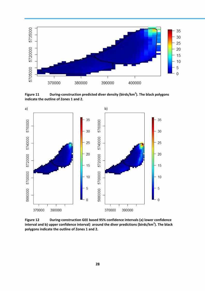
28

Figure 11 During-construction predicted diver density (birds/km2). The black polygons indicate the outline of Zones 1 and 2.

a) b)

Figure 12 During-construction GEE based 95% confidence intervals (a) lower confidence interval and b) upper confidence interval) around the diver predictions (birds/km2). The black polygons indicate the outline of Zones 1 and 2.

29

Figure 13 Post-construction predicted diver density (birds/km2). The black polygons indicate the outline of Zones 1 and 2.

a) b)

Figure 14 Post-construction GEE based 95% confidence intervals (a) lower confidence interval and b) upper confidence interval) around the diver predictions (birds/km2). The black polygons indicate the outline of Zones 1 and 2.

30

Formal comparison for diver distribution between construction periods

Comparisons between construction periods were undertaken to assess if there had been a redistribution or reduction in diver numbers across the area of Zones 1 and 2. Differences were calculated as:

Pre-construction minus during-construction

Pre-construction minus post-construction

During-construction minus post-construction

There has been a significant decrease in diver numbers across most of Zones 1 and 2 between the pre-construction and during-construction phases (Figure 15). The greatest decline has been seen in the areas of highest density. This reduction is not localised to the wind farm footprint area and therefore is unlikely to have been caused by the construction of the wind farm.

Figure 15 Predicted differences in average diver numbers per 1 km x 1 km square between the pre- and during-construction phases (birds/km2) (former value minus latter value). Significant increases are indicated using ‘+’, while significant decreases are indicated using a ‘o‘. The centre of the London Array wind farm is indicated using ‘’ and the boundary is indicated by the grey polygon. The black polygons indicate the outline of Zones 1 and 2.

There appears to have been a redistribution of birds across the site between the pre-construction and post-construction phases within Zones 1 and 2 (Figure 16). Numbers are still significantly lower in the North East corner post-construction than they were in the pre-construction reference period, despite the average density between the two periods being similar (Figure 8). There has been an increase in numbers to the North of the wind farm and in the South West corner of Zone 2. These results are preliminary pending completion of the post-construction surveys however.

31

Figure 16 Predicted differences in average diver numbers per 1 km x 1 km square between the pre- and post- construction phases (birds/km2) (former value minus latter value). Significant increases are indicated using ‘+’, while significant decreases are indicated using a ‘o‘. The centre of the London Array wind farm is indicated using ‘’ and the boundary is indicated by the grey polygon. The black polygons indicate the outline of Zones 1 and 2.

There has been a significant increase in bird numbers post-construction when compared to the construction period within Zones 1 and 2 (Figure 17). Values across the site have increased, although there is a greater increase in numbers to the North East and South West corners of Zone 1 and 2 respectively.

32

Figure 17 Predicted differences in average diver numbers per 1 km x 1 km square between the during and post-construction phases (birds/km2) (former value minus latter value). Significant increases are indicated using ‘+’, while significant decreases are indicated using a ‘o‘. The centre of the London Array wind farm is indicated using ‘’ and the boundary is indicated by the grey polygon. The black polygons indicate the outline of Zones 1 and 2.

Relationship between diver density and distance to wind farm.

To investigate whether there is an effect of the wind farm on diver density, average diver densities as predicted from the GEE model were summarized for the wind farm, and for 1 km buffers extending around the wind farm up to 15 km distance in ArcGIS. The density of divers was calculated for each buffer and compared to that of the wind farm footprint. Confidence intervals calculated as part of the modelling process for each predicted value were used as a measure of uncertainty. This analysis does not take into account that there can be major differences in diver densities between years; therefore a lower density in a year does not necessarily mean that a local event in that year is the cause of that lower density. This important caveat also applies to the auk analyses described in Section 8.

The density of divers varied with distance to the London Array wind farm (Figure 18). There has been a decrease in density close to the wind farm during-construction years when compared to the pre-construction reference period. During-construction years, the density of divers is decreased compared to the pre-construction reference period up to at least 10 km from the wind farm. Post-construction, the density is more similar to that of the pre-construction reference period and is slightly higher, though not significantly so, within 2 km of the wind farm footprint. This does not account for any changes in abundance that could have occurred between the periods however.

33

Figure 18 Diver density at different distances from the London Array wind farm. Error bars show the 95% confidence intervals generated during the modelling process.

To look at how the distribution of divers between construction periods has changed, the proportion of diver density at each distance from the wind farm has been calculated (Figure 19). Whereas this is likely to provide a better indication of any effect that construction may have on the distribution of the divers, this analysis will only be valid for the density of divers present in each year. The results are not conclusive across all diver densities as the selection of habitat made by the divers will vary with habitat quality but this quality of habitat for foraging birds will vary with the number of divers on it (Fretwell & Lucas 1970, Fretwell 1972). Therefore in years of low diver densities the divers may select habitat with sufficient prey and also where real or perceived disturbance is low. Offshore wind farms or the boat traffic associated with the windfarms could be examples of such disturbance. However in years of high diver density, when competition for food between divers is greater, prey availability may become the key determinant of diver distribution and individual divers may become more tolerant of any real or perceived disturbance. Thus, any differences recorded in the observed proportions of divers with distance to the wind farm footprint should be taken to apply to the density of divers in that particular year, and any generalisation of the results should only be made with great caution. This important caveat also applies to the auk analyses described in Section 8.

0

5

10

15

20

25

30

0 0.5 1.5 2.5 3.5 4.5 5.5 6.5 7.5 8.5 9.5 10.5 11.5 12.5 13.5 14.5

Div

er

de

nsi

ty (

bir

ds

pe

r km

2)

Distance from London Array Wind Farm (km)

Diver density by distance to the London Array Wind Farm

Pre-construction

During construction

Post construction

34

Figure 19 Proportion of divers at different distances from the London Array wind farm. Error bars show the 95% confidence intervals generated during the modelling process.

Figure 19 shows that whilst there appears to be a redistribution of divers across the site between the years in each construction period, these differences are unlikely to be significant. There are fewer divers predicted to be present within 10 km of the wind farm during-construction, with an increase in the proportion of divers present outside of this distance. Post-construction, an increase in the proportion of divers is seen up to 5 km from the wind farm, when compared to the pre-construction reference period, with a decrease outside of this distance. A greater increase is seen when comparing the during-construction figures within 4.5 km of the wind farm to those of the post-construction period. These changes are highlighted when looking at the percentage change between these proportions in Figure 20.

0

0.02

0.04

0.06

0.08

0.1

0.12

0.14

0.16

0.18

0.2

0 0.5 1.5 2.5 3.5 4.5 5.5 6.5 7.5 8.5 9.5 10.5 11.5 12.5 13.5 14.5

Pro

po

rtio

n o

f d

ive

rs


Proportion of divers by distance from the London Array Wind Farm

Pre-construction

During construction

Post construction

35

Figure 20 Percentage change in proportion of divers at different distances from the London Array wind farm between construction periods. Error bars show the 95% confidence intervals generated during the modelling process.

-70

-50

-30

-10

10

30

50

70

90

110

130

150

0 0.5 1.5 2.5 3.5 4.5 5.5 6.5 7.5 8.5 9.5 10.511.512.513.514.5

Pe

rce

nta

ge c

han

ge (

%)


Percentage change in proportion of divers between construction periods

Pre/during construction

During/post construction

Pre/post constuction

36

8. Auk Model outputs

Not all auks were identified to species level, in particular in the early years of surveys. Therefore the modelling was carried out on the total of identified auks (razorbill, guillemot and puffin) and unidentified auk species.

Observed values of bird numbers per 1km2 grid cell across the years within each construction period within Zones 1 and 2 were plotted to give a visual indication of any change. This provided an average value across surveys within the years classified to each construction period (Figure 21).

a)

b)

c)

Figure 21 Observed Auk average numbers across each construction period within zones 1 and 2 for a) pre-construction years, b) during construction years, and c) post-construction years. The black polygons indicate the outline of Zones 1 and 2 and the white polygon the indicates the outline of the London Array windfarm. Figure axes are the area co-ordinates in UTMs.

37

Variables were assessed for co-linearity utilizing variance inflation factors prior to beginning the modelling process. This identified some co-linearity between variables and subsequently distance to coastline and wave base and wave force were removed from the variable list. All other variables listed in Table 7 were initially included within the model. Figure 22 shows the correlation between some of the initial variables.

Table 7 Starting adjusted GVIF values for the environmental variables initially considered within the modelling process for auks.

Model term GVIF^(1/(2*Df))

as.factor(Construction period) 1.032243

X coordinate 7.804969

Y coordinate 2.537693

Coast 2.48391

Aspect 1.108438

Slope 1.066768

Wave base 6.530648

Tidal base 2.399571

Bathymetry 1.933053

Tidal force 1.914426

Wave force 1.669285

Survey shipping 1.776228

Pre-survey shipping 1.765259

Chlorophyll a 1.118174

Sea surface temperature 1.347262

Thermal front probability 1.713539

38

Figure 22 Correlation between environmental variables.

Table 8 shows the final model after the SALSA 1D routine. Further model simplification and variable

assessment was undertaken utilising model p-values.

Table 8 Initial environmental variables p values used during model simplification

Model term DF P value

as.factor(Construction period) 2 1.82E-05

s(Bathymetry) 3 0.746451

s(Survey Shipping) 3 0.528914

s(Pre-survey Shipping) 4 0.000761

s(SST) 3 0.086616

s(tidal base) 3 0.01226

39

Spatially explicit modelling for auk species

Following model simplification only pre-survey shipping and tidal base remained in the 1D model, with X and Y co-ordinates being included within the 2D spatial smooth model. Figure 23 shows the ACF plot for auks, and the selected blocking structure. The final auk model is shown below:

Auks=geeglm(as.factor(Constrution period, Df=2) + s(Pre-survey Shipping, Df = 4) + s(tidal base, Df=3)), family=poisson)

Model dispersion parameter for the final auk model was 229.5. Model dispersion greater than 1 suggested that there is over dispersion and a large amount of noise (high variances in the count data) present in the underlying data. This supports the decision to fit an overdispersed model. Model diagnostics are shown in appendix I.

Model predictions for all areas surveyed including knot locations are shown in appendix II.

Figure 23 Auk model ACF plot. The grey lines show the model residuals whilst the red line shows the average autocorrelatoion. Autocorrelation between counts ceases when the red line stabilises at zero.

All variables included in the final model were significant at the 5% level (Table 9). Figure 24 and Figure 25 show the relationship between auks and the variables. These graphs show the modelled relationship between the response variables and the environmental variable. The vertical lines along the x-axis show the data points of the environmental variable.

40

Table 9 GEE based p-values for the terms in the auk model

Model term p-value

Construction period <0.0001

Spatial smoother <0.0001

Pre-survey shipping <0.0001

Tidal base 0.0264

Construction period:spatial smoother interaction <0.0001

Figure 24 Fitted pre-survey shipping relationship with GEE based 95% confidence intervals for auks.

41

Figure 25 Fitted tidal base relationship with GEE based 95% confidence intervals for auks.

Estimated density of auks across phases

Estimated average densities of auks were lower during-construction years than pre- or post- construction years for both Zones 1 and 2 and within the London Array wind farm footprint.(Figure 26). Predicted densities within the windfarm post-construction years still showed a lower estimate than pre-construction years, although this change may not be significant. Predicted numbers of auks varied between construction phases although all showed an increased density of auks in the north east corner of Zone 1 (Figure 27, Figure 29, Figure 31). This pattern of distribution was also reflected in the confidence intervals around the model predictions (Figure 28, Figure 30, Figure 32). Within the post-construction years in Zones 1 and 2, numbers have exceeded the numbers recorded pre-construction due to an increased number of auks being predicted in the South of the site (Figure 31). These results are preliminary however, pending the final year of post-construction surveys. Auk density decreased during-construction when compared with pre-construction values.

42

a)

b)

Figure 26 Average density of auks across construction periods for a) Zones 1 and 2, and b) within the London Array wind farm footprint only. Error bars show average 95% confidence intervals generated from the model predictions.

.

0

1

2

3

4

5

6

Pre-construction During-construction Post-construction

Au

k d

en

sity

(b

ird

s p

er

km2)

0

1

2

3

4

5

6

Pre-construction During-construction Post-construction

Au

k d

en

sity

(b

ird

s p

er

km2 )

43

Figure 27 Pre-construction predicted auk density (birds/km2). The black polygons indicate the outline of Zones 1 and 2.

a) b)

Figure 28 Pre-construction GEE based 95% confidence intervals (a) lower confidence interval and b) upper confidence interval) around the auk predictions (birds/km2). The black polygons indicate the outline of Zones 1 and 2.

44

Figure 29 During-construction predicted auk density (birds/km2). The black polygons indicate the outline of Zones 1 and 2.

a) b)

Figure 30 During-construction GEE based 95% confidence intervals (a) lower confidence interval and b) upper confidence interval) around the auk predictions (birds/km2). The black polygons indicate the outline of Zones 1 and 2.

45

Figure 31 Post-construction predicted auk density (birds/km2). The black polygons indicate the outline of Zones 1 and 2.

a) b)

Figure 32 Post-construction GEE based 95% confidence intervals (a) lower confidence interval and b) upper confidence interval) around the auk predictions (birds/km2). The black polygons indicate the outline of Zones 1 and 2.

46

Formal comparison for auk distribution between construction periods

Comparisons between construction period years were undertaken to assess if there had been a redistribution or reduction in auk numbers across the area. Differences were calculated as:

Pre-construction minus during-construction

Pre-construction minus post-construction

During-construction minus post-construction

There has been a significant decrease in auk numbers across most of Zones 1 and 2 before construction and during-construction (Figure 33). There has been a significant decline in auks predicted in and around the London Array wind farm with a significant increase in auks predicted on the Eastern outskirts of Zone 1.

Figure 33 Predicted differences in average auk numbers per 1km x 1 km square comparing pre- and during-construction (birds/km2) (former value minus latter value). . Significant increases are indicated using ‘+’, while significant decreases are indicated using a ‘o‘. The centre of the London Array wind farm is indicated using ‘’ and the boundary is indicated by the grey polygon. The black polygons indicate the outline of Zones 1 and 2.

There appears to have been a redistribution of birds across the site between the pre-construction and post-construction phases (Figure 34). Numbers are still significantly lower in and around the London Array wind farm during the post-construction years than they were in the pre-construction reference period. There has been a significant increase in numbers to the North of the wind farm and in the South West corner of Zone 2. These results are preliminary pending completion of the post-construction surveys.

There has been a significant increase in bird numbers post-construction when compared to the construction period years (Figure 35). There are widespread increases across the site, although significant decreases are shown in the South East corner of Zone 1.

47

Figure 34 Predicted differences in average auk numbers per 1 km x 1 km square comparing pre- and post-construction (birds/km2) (former value minus latter value). . Significant increases are indicated using ‘+’, while significant decreases are indicated using a ‘o‘. The centre of the London Array wind farm is indicated using ‘’ and the boundary is indicated by the grey polygon. The black polygons indicate the outline of Zones 1 and 2.

48

Figure 35 Predicted differences in average auk numbers per 1 km x 1 km square comparing during- and post-construction (birds/km2) (former value minus latter value). . Significant increases are indicated using ‘+’, while significant decreases are indicated using a ‘o‘. The centre of the London Array wind farm is indicated using ‘’ and the boundary is indicated by the grey polygon. The black polygons indicate the outline of Zones 1 and 2.

Relationship between auk density and distance to wind farm.

To investigate if there is an effect of the wind farm on auk density, average auk density was summarized for the wind farm, and for 1 km buffers extending around the wind farm up to 15 km distance. The density of auks was calculated for each buffer and compared. The caveats as discussed within section 7 also apply to the following analysis. The density of auks varied with distance to the London Array wind farm (Figure 36). There has been a decrease in density close to the wind farm in both during and post-construction periods. During-construction years, the density of auks matches that of the pre-construction reference period from approximately 8.5 km from the wind farm. Post-construction years, the density matches that of the pre-construction reference period at approximately 5.5 km from the wind farm. This does not account for changes in abundance between periods however. The results have not been subjected to statistical analysis but visually do not appear to indicate a significant change. To look at how the distribution of auks between construction periods has changed, the proportion of auk density at each distance from the wind farm has been calculated (Figure 37).

49

Figure 36 Auk density at different distances from the London Array wind farm. Error bars show the 95% confidence intervals generated during the modelling process.

Figure 37 Proportion of auks at different distances from the London Array wind farm. Error bars show the 95% confidence intervals generated during the modelling process.

0

2

4

6

8

10

12

14

16

0 0.5 1.5 2.5 3.5 4.5 5.5 6.5 7.5 8.5 9.5 10.5 11.5 12.5 13.5 14.5

Au

k d

en

sity

(b

ird

s p

er

km2)

Distance from London Array Wind Farm (Km)

Auk density by distance to the London Array Wind Farm

Pre-construction

During construction

Post construction

0

0.05

0.1

0.15

0.2

0.25

0 0.5 1.5 2.5 3.5 4.5 5.5 6.5 7.5 8.5 9.5 10.5 11.5 12.5 13.5 14.5

Pro

po

rtio

n o

f au

k

Distance from London Array Wind Farm (Km)

Proportion of Auk by distance to the London Array Wind Farm

Pre-construction

During construction

Post construction

50

Figure 37 indicates there has been a redistribution of auks across the site between the construction period years although these changes are unlikely to be significant. There are fewer auks predicted within 4 km of the wind farm during-construction, with an increase in auk number outside of this distance. Post-construction years, a decrease in the proportion of auks is seen up to 7 km from the wind farm, when compared to the pre-construction reference period, with an increase outside of this distance. These changes are highlighted when looking at the percentage change between these proportions in Figure 38.

Figure 38 Percentage change in proportion of auks at different distances from the London Array wind farm between construction periods. Error bars show the 95% confidence intervals generated during the modelling process.

-85

-65

-45

-25

-5

15

35

55

75

95

115

135

155

0 0.5 1.5 2.5 3.5 4.5 5.5 6.5 7.5 8.5 9.5 10.5 11.5 12.5 13.5 14.5

Pe

rce

tage

ch

ange

(%

)


Percentage change in proportion of auks between construction periods

Pre/during construction

During/post construction

Pre/post constuction

51

9. Discussion

This report details the methods and steps taken to develop a statistically robust approach to undertake spatial modelling to detect any change between construction periods in the Outer Thames Estuary SPA. This approach has been used on both divers and auks to determine any statistically significant changes in numbers or redistribution within the site. Analysis followed the CReSS/SALSA method developed by St Andrew’s University, as recommended for offshore data (Mackenzie et al. 2013). As data collection is yet to be completed for the post-construction phase, this discussion will focus on the pre-construction and during-construction changes.

The datasets used within this model are spatially and temporally complex. The requirement was to develop an analysis approach that enabled all of the data that were suitable and available to be used in the model building stage. This novel approach has allowed more data to be used to build the models to provide greater confidence in the model outputs. This method is suitable to allow inclusion of additional post-construction data in future.

Initial models were constructed with a large number of continuous variables, but during the model

simplification process these were reduced to two variables in both the diver (Table 6) and the auk

(Table 9) models. In both models a metric of shipping activity was retained. The activity of shipping

vessels on the days the survey was carried out contributed to explaining the diver distribution

(P<0.0001), whilst the shipping activity on the days preceding the survey contributed to explaining

the auk distribution (P<0.0001). This would suggest that both species are disturbed by the presence

of shipping vessels but this disturbance has a longer effect on auks.

Both divers and auks showed a reduction in numbers during the construction period when compared to the pre-construction reference period. Whilst there was an overall reduction in average density for both the divers and the auks, there was also an indication that there had been redistribution across the site. Divers appeared to avoid the areas within 9 km of the offshore wind farm during the construction period (Figure 20) whilst auks only avoided areas up to approximately 4 km from the wind farm (Figure 38). This may suggest that divers are more sensitive to the construction effects of an offshore wind farm than auks, but it must be noted that the proportional decline in auk numbers is greater than that of divers near the windfarm. These results have not been subjected to any statistical analysis and therefore may not indicate significant changes.

Looking at how the proportion of birds at different distances from the wind farm change is likely to provide a better indication of any effect that construction may have on the distribution of the birds rather than looking at changes in absolute density as the latter analysis will only be valid for the density of each species present in each year. The results are not conclusive across all densities which may be because the selection of habitat made by the birds will vary with habitat quality, but this quality of habitat for foraging birds will also vary with the number of birds on it (Fretwell & Lucas 1970, Fretwell 1972). Therefore in years of low bird densities the birds may select habitat with sufficient prey and also where real or perceived disturbance is low. Offshore wind farms or the boat traffic associated with the windfarms could be examples of such disturbance. However in years of high bird density, when competition for food between birds is greater, prey availability may become the key determinant of bird distribution and individual birds may become more tolerant of any real or perceived disturbance. Thus, any differences recorded in the observed proportions of birds with

52

distance to the wind farm footprint should be taken to apply to the density of birds in that particular year, and any generalisation of the results should only be made with great caution.

Initial analysis of the post-construction data however, shows some marked differences between the divers and the auks. Whilst numbers appear to return to pre-construction levels (as shown by the average density between construction periods) for both the auks and divers, the distribution has altered particularly for the auks. During the first post-construction year, there are still proportionally fewer auks in the wind farm and surrounding area up to approximately 7 km from the wind farm. In that same year, divers appear to return to their pre-construction distribution suggesting that the disturbance is short-lived and confined to the construction period. These results are preliminary however, as post-construction survey data collection was still on-going at the commencement of this project.

Overall it has been demonstrated that the CReSS/SALSA method provides a suitable model framework on which to base further analysis of this ongoing dataset. However, further developments (suggested below) and incorporating additional post-construction data will allow more definite conclusion on the effect of the wind farm construction to be ascertained.

10. Future developments

This report has detailed the steps taken to develop a modelling framework for future analysis of data within the Outer Thames estuary. Whilst the method detailed here provides a sound methodology for undertaking future analysis, there are a number of areas that are worth considering and investigating which are detailed below.

Incorporating additional post-construction data from the London Array wind farm area would strengthen the models considerably and allow a proper interpretation of changes post-construction to be undertaken.

In addition, incorporating power analysis within the model checking procedures may identify the strength of any associations between variables.

During the modelling process, it would be interesting to carry out a comparison to identify the effect of utilising different fit measures e.g. bic, aic, CV, p values, for model selection, to see how these would affect the final model, the environmental variables that are kept in the model and the model predictions. It may also be beneficial to explore the effect of utilising different cut-off values for the co-linearity tests to see how this affects final model selection.

An area that may require further in depth analysis would be to compare the effect on the final models when all the data has been used to build the model (as shown in this report) or just the data contained within zones 1 and 2. This may have implications for the placements of knots and areas of flexibility that may enhance the ability of the model to detect small changes.

One further area for consideration is to use a 500m grid resolution instead of a 1km grid. If the resolutions of the environmental variables are at a greater level than 1km than additional flexibility may be incorporated by using a 500m grid that may allow more subtle changes to be predicted. These points may help to enhance the models further.

53

11. References

APEM Ltd (2010). London Array OWF Aerial Bird Winter Survey 2009-10. APEM Scientific Report, August 2010. Final. 40 pp.

APEM Ltd (2013). Aerial bird surveys in the Outer Thames Estuary SPA. APEM Scientific Report for Natural England, July 2013, Final. 67 pp.

Camphuysen, K.J., Fox, A.D., Leopold M.F. & Petersen, I.K. (2004). Towards standardised seabirds at sea census techniques in connection with environmental impact assessments for offshore wind farms in the U.K. Report commissioned by COWRIE Ltd for The Crown Estate. Royal Netherlands Institute for Sea Research, Texel, 38 pp.

Cramp, S. & Simmons, K.E.L. (1977) The Birds of the Western Palearctic, Vol. I. Oxford University Press, Oxford.

DTI (2006). Aerial Surveys of Waterbirds in Strategic Windfarm Areas: 2004/05 Final Report. DTI, London.

Fretwell, S. D. & Lucas, H.L. (1970) On territorial behavior and other factors influencing habitat distribution in birds. I. Theoretical development. Acta Biotheoretica 19, 16–36

Fretwell, S.D. (1972) Populations in a seasonal environment. Princeton University Press, Princeton, N.J.

Furness, B. (2013). Extent of displacement, and mortality implications of displacement of seabirds by offshore wind farms. Draft Environmental Statement Chapter 11 Appendix B Seabird Displacement Review. 22 pp.

Garthe, S. & Hüppop, O 2004. Scaling possible adverse effects of marine wind farms on seabirds: developing and applying a vulnerability index. Journal of Applied Ecology 41, 724–734

Hardin, J. and Hilbe, J., 2002. Generalized Estimating Equations. Chapman and Hall, CRC Press.

Hastie, T., Tibshirani, R. and Friedman, J. 2009. The elements of statistical learning. 2nd edition. Springer. Mackenzie, M.L., Scott-Hayward, L.A., Oedekoven, C.S., Skov, H., Humphreys, E. & Rexstad, E. (2013). Statistical Modelling of Seabird and Cetacean data: Guidance Document. University of St. Andrews contract for Marine Scotland; SB9 (CR/2012/05). 196pp.

Leopold, M.F., Dijkman, E.M., Teal, L & the OWEZ-team (2011). Local Birds in and around the Offshore Wind Farm Egmond aan Zee (OWEZ) (T-0 & T-1, 2002-2010). NoordzeeWind report OWEZ_R_221_T1_20110915_localbirds_final. Imares / NoordzeeWind, Wageningen / IJmuiden.

Lyngs, P. and Kampp, K. (1996). Ringing recoveries of razorbills Alca torda and guillemots Uria aalge in Danish waters. Dansk Ornitologisk Forenings Tidsskrift 90, 119-132.

54

Mackenzie, M.L, Scott-Hayward, L.A.S., Oedekoven, C.S., Skov, H., Humphreys, E., and Rexstad E. (2013). Statistical Modelling of Seabird and Cetacean data: Guidance Document. University of St. Andrews contract for Marine Scotland; SB9 (CR/2012/05).

Maclean, I.M.D., Skov, H. & Rehfisch, M.M. 2007. Further use of aerial surveys to detect displacement at offshore wind farms. BTO research Report No. 482 to COWRIE. BTO, Thetford.

Percival, S. (2010). Kentish Flats Offshore Wind Farm: Diver Surveys 2009-10. Report for Vattenfall Wind Power. 31pp.

Petersen, I.K., Nielsen, R.D. & Mackenzie, M.L. (2014) Post-construction evaluation of bird abundances and distributions in the Horns rev 2 offshore wind farm, 2011 and 2012. Report commissioned by DONG Energy. Aarhus University & DCE - Danish Centre for Environment & Energy. 51 pp.

Piatt, J.F. & Nettleship, D.N. 1985. Diving depths of four alcids. Auk 102, 293–297.

Rexstad, E. and Buckland, S.T., 2012. Displacement analysis boat surveys Kentish Flats. Report by CREEM, University of St Andrews to Strategic Ornithological Support Services (SOSS): SOSS 1A Displacement http://www.bto.org/sites/default/files/u28/downloads/Projects/Final_Report_SOSS01A.pdf.

R Core Team (2014). R: A language and environment for statistical computing. R Foundation for Statistical Computing, Vienna, Austria. URL http://www.R-project.org/.

Schwemmer, P., Mendel, B., Sonntag, N., Dierschke, V. & Garthe, S. (2011). Effects of ship traffic on seabirds in offshore waters: implications for marine conservation and spatial planning. Ecol Appl. 21, 1851-60.

Scott-Hayward, L.A.S., Oedekoven, C.S., MacKenzie, M.L., Walker, C.G., and Rexstad, E., 2013. User Guide for the MRSea Package: Statistical Modelling of bird and cetacean distributions in offshore renewables development areas. University of St. Andrews contract for Marine Scotland; SB9 (CR/2012/05).

Scott-Hayward, L.A.S., MacKenzie, M.L., Donovan, C.R., Walker, C.G., and Ashe, E., 2013. Complex Region Spatial Smoother (CReSS). Journal of Computational and Graphical Statistics, In press and online.

Skov, H. & Prins, E. (2001). Impact of estuarine fronts on the dispersal of piscivorous birds in the German Bight. Marine Progress Series 214, 279-287.

Skov, H., Heinänen, S., Lohier, S., Thaxter, C., Zydelis, R. & Stock, A. (2010). Modelling the abundance and area use of wintering red-throated divers in the Outer Thames Estuary. DHI draft report to London Array Ltd.

Stroud, D.A., Chambers, D., Cook, S., Buxton, N., Fraser, B., Clement, P., Lewis, I., McLean, I., Baker, H. & Whitehead, S. (2001). The UK SPA Network: its scope and content. Vols 1 – 3. JNCC, Peterborough.

http://www.r-project.org/

55

Walker, C., MacKenzie, M.L., Donovan, C.R., and O'Sullivan, M., 2011. SALSA – A Spatially Adaptive Local Smoothing Algorithm. Journal of Statistical Computation and Simulation. 81, 2.

Zuur, A.F., Ieno, E.N. & Smith, G.M. (2007). Analysing Ecologucal Data. Springer, USA

Zuur, A.F., Ieno, E.N., Walker, N., Saveliev, A.A. & Smith, G.M. (2009) Mixed Effects Models and Extensions in Ecology with R., Springer, USA.

56

12. Appendix I: Model diagnostics

Diver model

The following details the model checking that was undertaken for the diver model.

Figure 39 Plot of observed versus fitted values for the diver model

Figure 39 shows that high observed values are under-predicted, whilst observed zeros tend to be over-predicted (as it is unlikely they can be under-predicted). The marginal R-squared and concordance are low, which may suggest a poor model fit.

Figure 40 Plot of fitted values versus Pearsons residuals for the diver model

Figure 40 shows there is a possible pattern between the fitted values and the pearsons residuals but it is difficult to tell due to overplotting. The locally weighted least squares regression line does not indicate an unusual pattern and therefore there is no issue with model assumptions on the mean-variance relationship

57

a) b)

Figure 41 Plots of bathymetry for a) Cumulative residuals and b) runs tests for the diver model

Figure 41 shows that the cumulative residuals and runs plots suggest fewer runs than expected if the residuals were random (p<0.001) with a significant positive correlation when residuals were ordered by bathymetry. This suggests there is still some unmodelled correlation. The residuals show that the use of a GEE model was justified.

58

Figure 42 Raw residuals a) pre-construction, b) during-construction and c) post-construction. These residuals are fitted values – observed values (mean birds/km2) for the diver model.

The raw residuals (Figure 42) show good mixing of high and low values suggesting no real spatial pattern.

59

Figure 43 Raw residuals a) pre-construction, b) during-construction and c) post-construction for Zones 1 and 2 only. These residuals are fitted values – observed values (mean birds/km2) for the diver model.

60

Figure 44 Fit measure for the final GEE diver model. Blue bars indicate the range of the simulated data, the red line shows the fit of the final model.

Data were simulated from the model to look at the model fit based on the model being a “true” representation of the data. Figure 46 shows that the model fit based on the survey data falls within the range of the simulated data and therefore indicates the model is a good fit for the data.

61

Auk model

The following details the model checking that was undertaken for the auk model.

Figure 45 Plot of observed versus fitted values for the auk model

Figure 45 shows that high observed values are under-predicted, whilst observed zeros tend to be over-predicted (as it is unlikely they can be under-predicted). The marginal R-squared and concordance are low, which may suggest a poor model fit.

Figure 46 Plot of fitted values versus Pearsons residuals for the auk model

Figure 46 shows there is a possible pattern between the fitted values and the pearsons residuals but it is difficult to tell due to overplotting. The locally weighted least squares regression line does not indicate an unusual pattern and therefore there is no issue with model assumptions on the mean-variance relationship.

62

a) b)

Figure 47 Plots of tidal base for a) Cumulative residuals and b) runs tests for the auk model

63

Figure 47 shows that the cumulative residuals and runs plots suggest fewer runs than expected if the residuals were random (p<0.001) with a significant positive correlation when residuals were ordered by tidal base. This suggests there is still some unmodelled correlation, that will require a GEE to be used.

Figure 48 Raw residuals a) pre-construction, b) during-construction and c) post-construction. These residuals are fitted values – observed values (mean birds/km2) for the auk model.

The raw residuals (Figure 48) show no real spatial pattern to the residuals, and therefore there is no spatial bias in the model.

64

Figure 49 Raw residuals a) pre-construction, b) during-construction and c) post-construction for Zones 1 and 2 only. These residuals are fitted values – observed values (mean birds/km2) for the diver model.

65

Figure 50 Fit measure for the final GEE auk model. Blue bars indicate the range of the simulated data, the red line shows the fit of the final model.

Data were simulated from the model to look at the model fit based on the model being a “true” representation of the data. Figure 46 shows that the model fit based on the survey data falls within the range of the simulated data and therefore indicates the model is a good fit for the data.

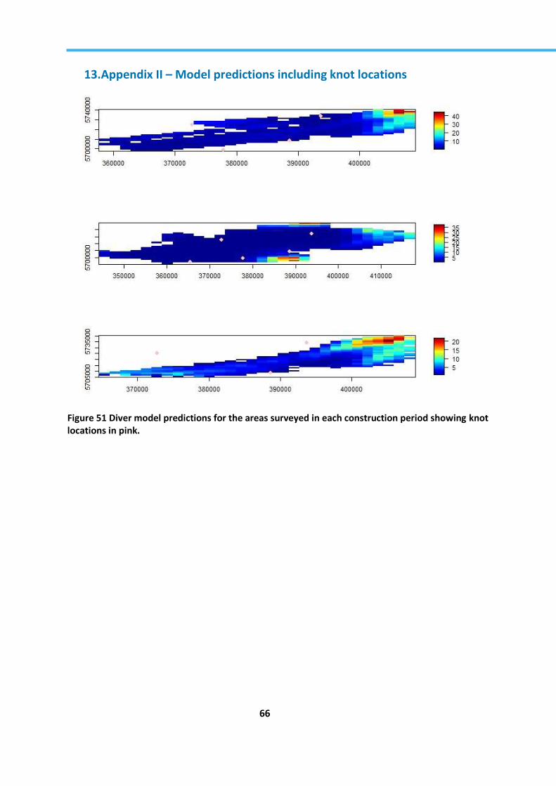
66

13. Appendix II – Model predictions including knot locations

Figure 51 Diver model predictions for the areas surveyed in each construction period showing knot locations in pink.

67

Figure 52 Auk model predictions for the areas surveyed in each construction period showing knot locations in pink.

68

14. Appendix III – Additional Model prediction plots

Figure 53 Diver model predictions on the same scale across construction periods

Figure 54 Diver model prediction confidence intervals on the same scale across construction periods

69

Figure 55 Auk model predictions on the same scale across construction periods

Figure 56 Auk model prediction confidence intervals on the same scale across construction periods

70

Figure 57 Diver model predictions on the log scale across construction periods

Figure 58 Diver model prediction confidence intervals on the log scale across construction periods

71

Figure 59 Auk model predictions on the log scale across construction periods

Figure 60 Auk model prediction confidence intervals on the log scale across construction periods

72

Figure 61 Proportion of divers predicted according to the final model across construction periods

Figure 62 Proportion of auks predicted according to the final model across construction periods

73

15. Appendix IV – R Code used in the modelling process

# Attach bird survey and environmental variables data

data$response<-data$T_diver

# poisson-based GLMs with and without a dispersion parameter estimate

(check if residual deviance is larger than residual degrees of freedom)

#impact alone

require(car)

glmFit1<-glm(round(T_diver)~Impact, data=data, offset=log(area),

family=poisson)

Anova(glmFit1)

glmFitOD1<- glm(round(T_diver)~Impact, data=data, offset=log(area),

family=quasipoisson)

Anova(glmFitOD1, test="F")

# Assess environmental variables for colinearity

fullModel<-glm(T_diver~as.factor(Impact) + x.pos + y.pos + Coast +

Aspect + Slope + Wave_base + tidal_base + Bathy + Tidal_force +

Wave_force + Survey_Shipping + Pre_survey_Shipping + Cla + SST + FF,

family = quasipoisson, data=data)

vif(fullModel)

variables<-data[c(7,8,14,15,16,17,18,19,20,21)]

panel.cor <- function(x, y, digits=2, prefix="", cex.cor, ...)

{

usr <- par("usr"); on.exit(par(usr))

par(usr = c(0, 1, 0, 1))

r <- abs(cor(x, y))

txt <- format(c(r, 0.123456789), digits=digits)[1]

txt <- paste(prefix, txt, sep="")

if(missing(cex.cor)) cex.cor <- 0.8/strwidth(txt)

text(0.5, 0.5, txt, cex = cex.cor * r)

}

pairs(variables, lower.panel=panel.smooth, upper.panel=panel.cor)

# Remove variables until GVIF is less than 2

74

# Create foldid within the dataset to allow for Cross-validation

data$foldid<-getCVids(data, folds=5)

# Set initial model with factor terms

initialModel<-glm(response~as.factor(Impact)+ offset(log(area)),

family=quasipoisson, data=data)

# Set initial salsa list for all continuous variables.

salsa1dlist<-list(fitnessMeasure="QICb", minKnots_1d =

c(1,1,1,1,1,1,1,1,1,1), maxKnots_1d = c(5,5,5,5,5,5,5,5,5,5),

startKnots_1d=c(1,1,1,1,1,1,1,1,1,1), degree=c(2,2,2,2,2,2,2,2,2,2),

maxIterations=10, gaps=c(1,0.005,0.5,0.05,1,1,0.05,1,1,1))

# Set removal = TRUE to allow the SALSA routine to determine if

continuous variables showed remain within the model

salsa1dOutput<-runSALSA1D_withremoval(initialModel, salsa1dlist,

c("Aspect", "Slope", "Bathy", "Tidal_force", "Survey_Shipping",

"Pre_survey_Shipping", "Cla", "SST", "FF", "Wave_force"),

predictionData=enviro.data, datain=data, removal=TRUE)

# Get the CV score for the best model.

getCV_CReSS(data, salsa1dOutput$bestModel, splineParams)

# Assess if the factor terms should remain. SALSA will not determine

automatic removal of factor terms

bestModel_factor_removed<- update(salsa1dOutput$bestModel, .~. -

as.factor(Impact))

getCV_CReSS(data, bestModel_factor_removed, splineParams)

require(splines)

Anova(salsa1dOutput$bestModel)

75

# Assess p values to dermine simplest model to take forward

#linear for Aspect?

bestModel<- update(salsa1dOutput$bestModel, .~. - bs(Aspect, knots =

splineParams[[2]]$knots, degree = splineParams[[2]]$degree,

Boundary.knots = splineParams[[2]]$bd)+Aspect)

Anova(bestModel)

# Create a knot grid using X and Y coordinate of the survey data

knotgrid<-getKnotgrid(coordData =cbind(data$x.pos, data$y.pos), numKnots

= 300, plot = T)

distMats <- makeDists(cbind(data$x.pos, data$y.pos), na.omit(knotgrid))

require(splines)

r_seq<-getRadiiChoices(10,distMats$dataDist)

# Set the initialModel to get the bestModel from the salsa 1D output

initialModel<-bestModel

# Set the salsa 2D model to include an interaction term of construction

phase with spatial smooth

salsa2dlist<-list(fitnessMeasure = 'QICb', knotgrid = knotgrid,

knotdim=c(100,100), startKnots=5, minKnots=2,

maxKnots=50, r_seq=r_seq, gap=0,

interactionTerm="as.factor(Impact)")

salsa2dOutput<-runSALSA2D(initialModel, salsa2dlist,

d2k=distMats$dataDist,k2k=distMats$knotDist,

splineParams=salsa1dOutput$splineParams)

# Check out results

updatedModel<- salsa2dOutput$bestModel

updatedModel<- update(updatedModel)

splineParams<- salsa2dOutput$splineParams

radii<- splineParams[[1]]$radii

aR <- splineParams[[1]]$invInd[splineParams[[1]]$knotPos]

radiusIndices<- splineParams[[1]]$radiusIndices

76

dists<- splineParams[[1]]$dist

# Ccheck blocking structure

acf(residuals(updatedModel, type="pearson"))

# Set a suitable blocking structure

data$id<-rep(1:ceiling(nrow(data)/30), each=30)[1:nrow(data)]

# Check the correlation decays

runACF(data$id, updatedModel)

data$foldid<-getCVids(data, folds=5, block='id')

# Create prediction grid for each construction period

enviro.data1<- enviro.data

enviro.data1$Impact<-1





#find out if there are any NA coefficients

colstodelete<-as.vector(which(is.na(coef(updatedModel))))

require(geepack)

# Set up intial gee Model using the best model from the SALSA 2D output

geeModel<- geeglm(formula(salsa2dOutput$bestModel), data=data,

family=poisson, id=id)

# Create a prediction grid for all construction periods

preddata<- rbind(enviro.data1,enviro.data2,enviro.data3)

77

# Create distances for the knot grid

dists<-makeDists(cbind(preddata$x.pos, preddata$y.pos),

na.omit(knotgrid),knotmat=FALSE)$dataDist

# Create predictions for all grid cells for all construction periods

preds<-predict.cress(preddata, splineParams, dists, geeModel)

# Assess the model and p values

summary(geeModel)

getPvalues(model=geeModel, varlist=c('Survey_Shipping', 'Bathy'),

factorlist='Impact')

# Assess the covariate relationship

par(mfrow=c(3,1))

runPartialPlots(model=geeModel, data=data, factorlist='Impact',

varlist=c('Survey_Shipping', 'Bathy'),showKnots=T )

# Check if an interation term for Impact is necessary

noint.model<-update(geeModel,.~.-

as.factor(Impact):LocalRadialFunction(radiusIndices, dists, radii, aR))

getPvalues(noint.model,varlist=c('Survey_Shipping', 'Bathy'),

factorlist='Impact')

# Assess model fit and run diagnostics

require(ggplot2)

runDiagnostics(geeModel)

# Plot cumulative residuals ordered by variables

require(lawstat)

78

plotCumRes(geeModel,varlist=c('Bathy'), splineParams=splineParams,

d2k=dists)

plotRunsProfile(geeModel, varlist=c('Bathy'))

plotCumRes(geeModel,varlist=c('Survey_Shipping'),

splineParams=splineParams, d2k=dists)

plotRunsProfile(geeModel, varlist=c('Survey_Shipping'))

# Plot model residuals for each construction period

resids<- data$T_diver-fitted(geeModel)

dims<-getPlotdimensions(data$x.pos, data$y.pos, 1000, 1000)

par(mfrow=c(3,1), mar=c(3,3,3,5))

quilt.plot(data$x.pos[data$Impact==1],

data$y.pos[data$Impact==1],resids[data$Impact==1], ncol=dims[2],

nrow=dims[1], zlim=c(-2.2, 2.2))







require(calibrate)

# Assess the Covratio and Press statistics

timeInfluenceCheck(geeModel, id = data$blockid, d2k = dists,

splineParams = splineParams)

runInfluence(model = geeModel, id = data$blockid, d2k = dists,

splineParams = splineParams)

#fitted values

require(fields)

par(mfrow=c(3,2))

quilt.plot(data$x.pos[data$Impact==1], data$y.pos[data$Impact==1],

fitted(geeModel)[data$Impact==1], xlim=range(data$x.pos),

ylim=range(data$y.pos))

79







#plotting predictions without deleting areas that werent surveyed.

par(mfrow=c(3,1))

quilt.plot(preddata$x.pos[preddata$Impact==1],

preddata$y.pos[preddata$Impact==1],

preds[preddata$Impact==1],nrow=50, ncol=50)

points(na.omit(knotgrid)[aR,], pch=20, cex=2 , col="pink")



preds[preddata$Impact==2], nrow=50, ncol=50)

points(na.omit(knotgrid)[aR,], pch=20, cex=2,col="pink")



preds[preddata$Impact==3], nrow=50, ncol=50)

points(na.omit(knotgrid)[aR,], pch=20, cex=2, col="pink")

#removing predictions for areas that weren’t surveyed in each impact

phase.

require(splancs)

#read in polygons

pre<-read.csv("Pre_construction_points.csv")

dur<-read.csv("During_construction_points.csv")

post<-read.csv("post_construction_points.csv")

predin<- c()

par(mfrow=c(3,2))

for(i in unique(pre$Zone)){

print(i)

80

p<-cbind(pre[,2][pre$Zone==i], pre[,3][pre$Zone==i])

p<- rbind(p,p[1,])

lines(p, lwd=2, col="pink")

predin<- cbind(predin,ifelse(inout(cbind(preddata$x.pos,

preddata$y.pos),p),1,0))

}

predin2<- c()

p<-cbind(dur[,1], dur[,2])

p<- rbind(p,p[1,])

lines(p, lwd=2, col="blue")

predin2<- cbind(predin2,ifelse(inout(cbind(preddata$x.pos,


predin3<- c()

plot(preddata$x.pos, preddata$y.pos)

for(i in unique(post$Zone)){

print(i)

p<-cbind(post[,2][post$Zone==i], post[,3][post$Zone==i])

p<- rbind(p,p[1,])

lines(p, lwd=2, col="red")

predin3<- cbind(predin3,ifelse(inout(cbind(preddata$x.pos,


}

predsin1<- ifelse(apply(predin,1,sum)==1 & preddata$Impact==1,1,0)

predsin2<- ifelse(apply(predin2,1,sum)==1 & preddata$Impact==2,1,0)

predsin3<- ifelse(apply(predin3,1,sum)==1 & preddata$Impact==3,1,0)

rowstokeep<- c(which(predsin1==1), which(predsin2==1),

which(predsin3==1))

preddata2<- preddata[rowstokeep,]

preds2<- preds[rowstokeep]

81

# Plotting predictions with knots

par(mfrow=c(3,1))

quilt.plot(preddata2$x.pos[preddata2$Impact==1],

preddata2$y.pos[preddata2$Impact==1],

preds2[preddata2$Impact==1],nrow=30, ncol=30)










#Load in prediction grid for clipped area

preddata_clip<-read.csv("preddata_clip.csv")

#Create new dists for clipped area

dists<-makeDists(cbind(preddata_clip$x.pos, preddata_clip$y.pos),

na.omit(knotgrid) )$dataDist

# Predict using clipped area

preds2<-predict.cress(preddata_clip, splineParams, dists, geeModel)

# Create 95% confidence intervals for clipped area predictions

do.bootstrap.cress(data, preddata_clip, ddf.obj=NULL, geeModel,

splineParams,

g2k=dists, resample='id', rename='segment.id',

stratum=NULL,

82

B=1000, name="cress", save.data=FALSE, nhats=FALSE)

load("cresspredictionboot.RData")

head(bootPreds)

cis<-makeBootCIs(bootPreds)

#make prediction data

differences1_2<-

getDifferences(beforePreds=bootPreds[preddata_clip$Impact==1,],

afterPreds=bootPreds[preddata_clip$Impact==2,])

differences1_3<-



differences2_3<-



mediandiff1_2<-differences1_2$mediandiff



#The marker for each after-before differences: positive ('1') and

negative ('-') significant differences

marker1_2<-differences1_2$significanceMarker



par(mfrow=c(1,1))

quilt.plot(preddata_clip$x.pos[preddata_clip$Impact==1],

preddata_clip$y.pos[preddata_clip$Impact==1],

83

mediandiff1_2, nrow=30, ncol=30)

points(preddata_clip$x.pos[preddata$Impact==1][marker1_2==1],

preddata_clip$y.pos[preddata$Impact==1][marker1_2==1],

pch="+", col="darkgrey", cex=0.75)

points(preddata_clip$x.pos[preddata$Impact==1][marker1_2==(-1)],

preddata_clip$y.pos[preddata$Impact==1][marker1_2==(-1)],

col="darkgrey", cex=0.75)

points(395915.505897,5720464.155230, cex=3, pch="*", lwd=1, col="grey")



mediandiff1_3, asp=1, nrow=30, ncol=30)










mediandiff2_3, asp=1, nrow=30, ncol=30)








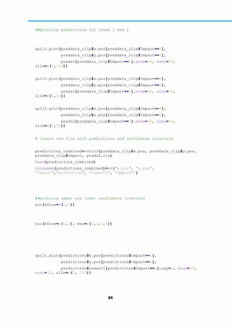
84

##plotting predictions for zones 1 and 2



preds2[preddata_clip$Impact==1],nrow=30, ncol=30,

zlim=c(0,100))




zlim=c(0,36))




zlim=c(0,30))

# Create new file with predictions and confidence intervals

predictions_combined<-cbind(preddata_clip$x.pos, preddata_clip$y.pos,

preddata_clip$Impact, preds2,cis)

head(predictions_combined)

colnames(predictions_combined)<-c("x.pos", "y.pos",

"Impact","prediction", "lowerCI", "upperCI")

##plotting upper and lower confidence intervals

par(mfrow=c(1,2))

par(mfrow=c(1,2), mar=c(3,3,3,5))

quilt.plot(predictions$x.pos[predictions$Impact==1],

predictions$y.pos[predictions$Impact==1],

predictions$lowerCI[predictions$Impact==1],asp=1, nrow=30,

ncol=30, zlim=c(0, 100))

85



predictions$upperCI[predictions$Impact==1],asp=1, nrow=30,

ncol=30, zlim=c(0, 100))




ncol=30, zlim=c(0, 36))




ncol=30, zlim=c(0, 36))




ncol=30, zlim=c(0, 30))




ncol=30, zlim=c(0, 30))

assessment of displacement impacts of offshore windfarms

Documents