assessing water quality modeling in subtropical regions
TRANSCRIPT

Brigham Young University Brigham Young University
BYU ScholarsArchive BYU ScholarsArchive
Theses and Dissertations
2008-12-03
Assessing Water Quality Modeling in Subtropical Regions Based Assessing Water Quality Modeling in Subtropical Regions Based
on a Case Study of the Aguamilpa Reservoir on a Case Study of the Aguamilpa Reservoir
Oliver Obregon Brigham Young University - Provo
Follow this and additional works at: https://scholarsarchive.byu.edu/etd
Part of the Civil and Environmental Engineering Commons
BYU ScholarsArchive Citation BYU ScholarsArchive Citation Obregon, Oliver, "Assessing Water Quality Modeling in Subtropical Regions Based on a Case Study of the Aguamilpa Reservoir" (2008). Theses and Dissertations. 1622. https://scholarsarchive.byu.edu/etd/1622
This Thesis is brought to you for free and open access by BYU ScholarsArchive. It has been accepted for inclusion in Theses and Dissertations by an authorized administrator of BYU ScholarsArchive. For more information, please contact [email protected], [email protected].

ASSESSING WATER QUALITY MODELING IN SUBTROPICAL
REGIONS BASED ON A CASE STUDY OF
THE AGUAMILPA RESERVOIR
by
Oliver Obregon
A thesis submitted to the faculty of
Brigham Young University
in partial fulfillment of the requirements for the degree of
Master of Science
Department of Civil and Environmental Engineering
Brigham Young University
December 2008


BRIGHAM YOUNG UNIVERSITY
GRADUATE COMMITTEE APPROVAL
of a thesis submitted by
Oliver Obregon This thesis has been read by each member of the following graduate committee and by majority vote has been found to be satisfactory. Date E. James Nelson, Chair
Date Gustavious P. Williams
Date M. Brett Borup

BRIGHAM YOUNG UNIVERSITY As chair of the candidate’s graduate committee, I have read the thesis of Oliver Obregon in its final form and have found that (1) its format, citations, and bibliographical style are consistent and acceptable and fulfill university and department style requirements; (2) its illustrative materials including figures, tables, and charts are in place; and (3) the final manuscript is satisfactory to the graduate committee and is ready for submission to the university library. Date E. James Nelson
Chair, Graduate Committee
Accepted for the Department
Steven E. Benzley Department Chair
Accepted for the College
Alan R. Parkinson Dean, Ira A. Fulton College of Engineering and Technology


ABSTRACT
ASSESSING WATER QUALITY MODELING IN SUBTROPICAL
REGIONS BASED ON A CASE STUDY OF
THE AGUAMILPA RESERVOIR
Oliver Obregon
Department of Civil and Environmental Engineering
Master of Science
The shortage of water in Mexico has made public and private institutions look at
reservoirs as an alternative solution for present and future water supply. However, eighty
percent of the existing reservoirs in Mexico are contaminated at some level, many
severely. Water quality models are water-management tools used to diagnose water
quality problems and the impact of various environmental conditions. They can be
effective in assessing various measures of remediation leading to improved water quality.
In most of the cases such water quality models have been successfully applied in
reservoirs located in temperate climates. However, the use of water quality models in
subtropical reservoirs, especially those in developing countries, have relatively little
application because either basic data are not available or because they are not sufficient.


In this study, a preliminary water quality model was developed for a subtropical
reservoir to assess both the ability to collect adequate data and the model’s underlying
applicability in a subtropical region. The Aguamilpa reservoir is located in the western
part of Mexico (Nayarit). It was built for power generation, irrigation and as a fishery.
CE-QUAL-W2 is a two-dimensional hydrodynamic and water quality model suitable for
long and narrow water bodies. Geometrically the Aguamilpa reservoir is long and deep,
making it an ideal candidate to be modeled by CE-QUAL-W2. The model was
developed for 1995 and 1996 because of a wider availability of historical data during this
period. In addition to a preliminary model and assessment of applicability in this
subtropical region, a monitoring and data acquisition plan was designed to identify the
minimum required data which must be used to update, calibrate and simulate the water
quality parameters. Once the model is calibrated, it may be used to simulate the water
quality changes occurring with respect to environmental, climatological and
anthropogenic effects. Further, the model may be used to prescribe operating procedures
upstream as well as at the dam which can serve to improve the overall water quality. The
development of the model at Aguamilpa can serve as a guideline for developing similar
water quality models in this and other similar subtropical locations.


ACKNOWLEDGMENTS
I wish to thank Dr. Jim Nelson for his trust and unconditional moral and
professional support. I also want to acknowledge the members of my committee, Dr.
Borup and Dr. Williams for their guidance. I thank the National Council of Science and
Technology (CONACYT) in Mexico for sponsoring this project and Jerry Miller, Nick
Williams and Clark Barlow for always sharing their modeling and field knowledge with
me. I wish to express my gratitude to Dr. Jose de Anda and CIATEJ for letting me
participate in the Aguamilpa project and for his advice and Gabriel Rangel for his field
assistance. I would like to thank Carlos Lecanda from CFE for his help in this project.
I owe a special debt of gratitude to my best friend, my wife Edith, who always
encourages me to keep going and for her love. I also wish to thank my family for their
support, teachings, and love; especially to my dad, Angel Obregon, for helping me to get
field data.


vii
TABLE OF CONTENTS
LIST OF TABLES ....................................................................................................... xi
LIST OF FIGURES ................................................................................................... xiii
1 Introduction ...........................................................................................................1
1.1 Objectives ........................................................................................................2
1.2 Scope of the Study ...........................................................................................3
2 Background ............................................................................................................5
2.1 Study Site Description ......................................................................................5
2.1.1 Hydrology ....................................................................................................6
2.1.2 Geology........................................................................................................8
2.1.3 Climatology..................................................................................................9
2.1.4 Power Generation ....................................................................................... 10
2.2 Water Quality Issues ...................................................................................... 12
2.3 Water Quality Models .................................................................................... 13
2.3.1 AQUATOX ................................................................................................ 14
2.3.2 EPDRiv1 .................................................................................................... 15
2.3.3 WASP7 ...................................................................................................... 15
2.3.4 QUAL2K ................................................................................................... 16
2.3.5 CE-QUAL-W2 ........................................................................................... 16
2.4 Model Selection ............................................................................................. 17
2.4.1 CE-QUAL-W2 Versions ............................................................................ 18

viii
2.4.2 CE-QUAL-W2 Capabilities and Limitations .............................................. 19
2.5 Subtropical Reservoirs ................................................................................... 21
2.5.1 Stratification .............................................................................................. 21
2.5.2 Eutrophication ........................................................................................... 23
3 Model Development ............................................................................................. 25
3.1 Bathymetry .................................................................................................... 25
3.2 Initial Conditions ........................................................................................... 31
3.3 Meteorological File........................................................................................ 32
3.4 Boundary Conditions ..................................................................................... 33
3.4.1 Inflows....................................................................................................... 33
3.4.2 Outflows .................................................................................................... 34
3.4.3 Inflow Temperatures .................................................................................. 35
3.4.4 Inflow Constituents .................................................................................... 35
3.4.5 Distributed Tributary Files ......................................................................... 36
3.5 Data Gaps ...................................................................................................... 37
3.5.1 Meteorological Adjustments ...................................................................... 37
3.5.2 Boundary Condition Modifications ............................................................ 40
4 Results .................................................................................................................. 43
4.1 Water Balance Calibration ............................................................................. 43
4.2 Thermal Simulation ....................................................................................... 46
4.3 Example Water Quality Simulations .............................................................. 48
4.4 Monitoring and Data Acquisition Plan ........................................................... 52
5 Summary and Conclusions .................................................................................. 55
References.................................................................................................................... 59
Appendix A. Scheme of the Aguamilpa-Solidaridad Dam ..................................... 65

ix
Appendix B. Bathymetry .......................................................................................... 67
Appendix C. Control File ......................................................................................... 71
Appendix D. CFE Dams and Gauging Stations Location ....................................... 87

x
xi
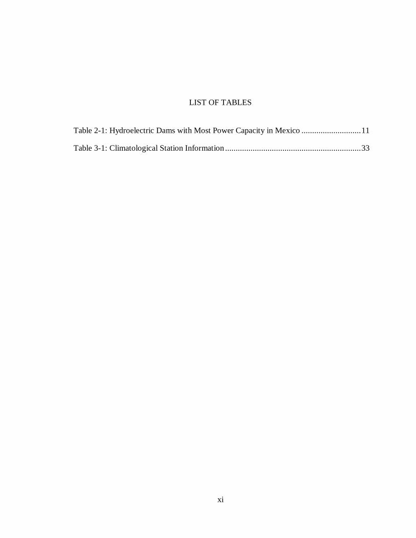
LIST OF TABLES Table 2-1: Hydroelectric Dams with Most Power Capacity in Mexico ............................ 11
Table 3-1: Climatological Station Information ................................................................ 33

xii

xiii
LIST OF FIGURES
Figure 2-1: Aguamilpa Reservoir and Aguamilpa-Solidaridad Dam, Nayarit, Mexico (INP, 2006) ......................................................................................................... 6
Figure 2-2: Main Watersheds Surrounding the Aguamilpa Reservoir (Potential Impacts, 2003) .................................................................................................................. 7
Figure 2-3: Rainfall in mm/yr of the Lerma-Chapala-Santiago Watershed (Potential Impacts, 2003) .................................................................................................... 8
Figure 2-4: Types of Climates in Nayarit, Mexico (INEGI, 2007) ................................. 10
Figure 2-5: Reservoir Stratification ............................................................................... 22
Figure 3-1: TIN of the Aguamilpa Reservoir Digitized by WMS .................................. 27
Figure 3-2: Branches and Segments of the Aguamilpa Reservoir ................................... 28
Figure 3-3: WMS Total Storage Capacity Curve vs. Field Data ..................................... 29
Figure 3-4: W2 Bathymetry Grid of Branch 1 (Santiago River) ..................................... 30
Figure 3-5: Location of Gauging Stations ...................................................................... 34
Figure 3-6: Tepic Air Temperatures and Aguamilpa Air Temperatures (Estimated) ....... 39
Figure 3-7: Air Temperature Analysis (Tepic-Carrizal) ................................................. 39
Figure 3-8: Air Temperature Data Used to Create Inflow Temperature Files ................ 42
Figure 4-1: Observed and Modeled Water Surface Elevations Comparison ................... 44
Figure 4-2: Water Balance Calibration of the Aguamilpa Reservoir .............................. 44
Figure 4-3: Water Temperature Simulation for Branch 1 (Santiago River) ..................... 47
Figure 4-4: Field vs. Modeled Water Temperature Data (1995) ..................................... 48
Figure 4-5: DO Example Simulation Branch 1 (Santiago River) .................................... 50
xiv
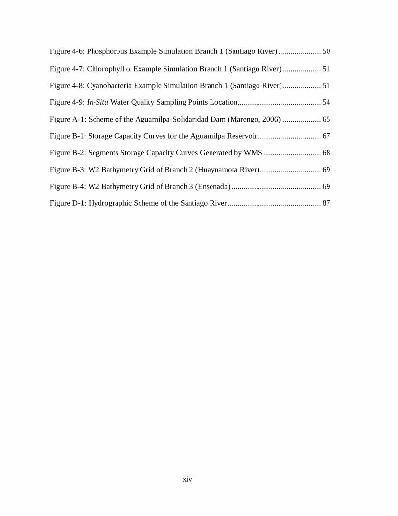
Figure 4-6: Phosphorous Example Simulation Branch 1 (Santiago River) ..................... 50
Figure 4-7: Chlorophyll α Example Simulation Branch 1 (Santiago River) ................... 51
Figure 4-8: Cyanobacteria Example Simulation Branch 1 (Santiago River) ................... 51
Figure 4-9: In-Situ Water Quality Sampling Points Location ......................................... 54
Figure A-1: Scheme of the Aguamilpa-Solidaridad Dam (Marengo, 2006) ................... 65
Figure B-1: Storage Capacity Curves for the Aguamilpa Reservoir ............................... 67
Figure B-2: Segments Storage Capacity Curves Generated by WMS ............................ 68
Figure B-3: W2 Bathymetry Grid of Branch 2 (Huaynamota River) .............................. 69
Figure B-4: W2 Bathymetry Grid of Branch 3 (Ensenada) ............................................ 69
Figure D-1: Hydrographic Scheme of the Santiago River .............................................. 87

1
1 Introduction
Lakes and reservoirs (natural or artificial) are key elements of water resources,
providing services for humans and a habitat for innumerable species of animals and
plants. In Mexico, artificial reservoirs have been built primarily to store large volumes of
water used for power generation, with secondary purposes being flood control, irrigation,
fishing, recreation, aquaculture and transportation. The shortage of water in Mexico has
made the National Power Commission (Comision Federal de Electricidad or CFE), the
National Water Commission (CONAGUA), and public/private institutions look at
reservoirs as an alternative solution for present and future domestic water supplies.
However, CONAGUA has reported that eighty percent of the four thousand five hundred
existing reservoirs in Mexico present different grades of pollution, many of which are
severe (Arredondo et al., 2008). This water quality degradation in reservoirs has been
caused by the intense use of fertilizers in agriculture, watershed modifications, land use
changes, introduction of exotic species, overfishing and untreated wastewater discharges.
The addition of nutrients such as phosphorous and nitrogen have classified most Mexican
reservoirs as eutrophic. Little is known about the reservoirs’ water quality conditions,
due to the fact that basic data either has not been collected or are insufficient (Huszar et
al., 2006). Moreover, management tools, such as water quality models, have not been
applied with great demand in Mexico because of the aforementioned reasons. Water

2
quality models have been successfully used in worldwide reservoirs located mostly in
temperate climates with a few cases in subtropical reservoirs to determine the water
quality management actions needed to reduce or eliminate water quality impairments.
Modeling sub-tropical reservoirs is a little or unexplored area. Aguamilpa reservoir,
located in the northwest region of Mexico, is an exceptional case study to show the
applicability of water quality models in sub-tropical zones. Considering the precedent
facts described above, the objectives and scope for this study are established.
1.1 Objectives
• Identify an adequate water quality modeling tool for a subtropical
reservoir using the Aguamilpa reservoir as a case study;
• Identify limitations and adjustments of the selected model;
• Determine how the selected water quality model is applicable in a
developing country like Mexico. Identify the sources of data available for
developing and using a water quality model;
• Develop an initial water quality model for the Aguamilpa reservoir using
existing data, supplemented with estimates in cases where gaps exist;
• Use results of the developed water quality model to refine a monitoring
and data acquisition plan that covers the gaps and extends the ability to
calibrate and use the model in a predictive nature.

3
1.2 Scope of the Study
This study is part of an important ongoing project titled “Development of a water
quality model for the Aguamilpa Dam (Nayarit),” sponsored by the National Council of
Science and Technology (CONACYT) in Mexico to evaluate water quality in the
Aguamilpa reservoir. This study is one part of a larger effort being coordinated by the
Center of Investigation and Advise in Technology and Design of the State of Jalisco
(CIATEJ). The other two research projects being done locally in Mexico are: 1) Water
quality temporal and spatial analysis; and 2) Hydrologic balance for the Aguamilpa
reservoir. The particular scope of this part of the ongoing project is to select and design
a water quality model while identifying gaps in available data and needs for monitoring
additional data.
An overview of water quality models and subtropical reservoirs is described.
Development of a water quality model for a subtropical reservoir (Aguamilpa) is
explained; describing the criteria used for the model selection, CE-QUAL-W2. A water
quality monitoring plan is defined from the developed model. The study also presents
results of the water balance calibration and water quality pre-simulations using sample
water quality constituents. Conclusions obtained from this model are explained and
future work is proposed to allow the improvement of a water quality model and its
application for reservoir management.

4
5
2 Background
2.1 Study Site Description
The Aguamilpa reservoir, located in the northwestern area of Mexico, was built
between 1989 and 1994 primarily to meet growing demands for electric energy, with
flood control, irrigation and fishery usage being secondary. The reservoir is part of the
Santiago and Huaynamota hydrologic system and it occupies approximately 60 km (37.3
miles) along the Santiago River, one of the most important and largest rivers in Mexico,
and 25 km (15.5 miles) along the Huaynamota River. The Aguamilpa-Solidaridad dam is
located in the state of Nayarit (104°46’29” longitude West and 21°50’32” latitude North),
52 km (32.3 miles) north from the capital city, Tepic (Figure 2-1). It is a rockfill dam
that stands 187 meters (613.5 feet) high and 642 meters (2,106.3 feet) long. At the time
of construction and until June 2005 the Aguamilpa dam was the highest concrete faced
rockfill dam operated in the world. It has a controlled-crest spillway structure, set at an
elevation of 210 meters (689.0 feet) above mean sea level. This structure was designed
for a peak flow of 17,900 m3/s (632,000.0 cfs) or 10000-year return period. According to
the International Commission on Large Dams (ICOLD), the Aguamilpa dam is classified

6
as a “large dam,” because it is higher than 15 meters (49.2 feet), and its spillway can
discharge over 2000 cubic meters per second (70,630.0 cfs) (IUCN and WB, 1997).
Figure 2-1: Aguamilpa Reservoir and Aguamilpa-Solidaridad Dam, Nayarit, Mexico (INP, 2006)
2.1.1 Hydrology
The Aguamilpa reservoir covers an area 109 km2 (26,935.0 acres) and the
conservation storage capacity of the reservoir is 5,540 Hm3 (4,491,350.0 acre-feet) of
water at the Maximum Ordinary Water Level (NAMO) elevation of 220 meters (720.8
feet). The maximum storage capacity of the reservoir is 6,950 Hm3 or 5,634,457.0 acre-
feet (approximately 4.5 times smaller than Lake Powell reservoir located in southeastern
Utah, US) at a Maximum Extraordinary Water Level (NAME) elevation of 232 meters
(760.0 feet). The Minimum Ordinary Water Level (NAMINO) elevation is found at 190
meters (623.0 feet), and the reservoir storages 2,965 Hm3 (2,403,765.0 acre-feet)

7
(Comision Federal de Electricidad [CFE], 1991). The drainage area to the Aguamilpa
reservoir is 73,834 km2 (18,244,780.0 acres), which represents 3.7% of the Mexican
territory and it has an annual average runoff (1949-2002) of 5,437 Hm3 (4,407,850.0
acre-feet) (CFE, 2002). There are 26 sub-basins of the Lerma-Chapala-Santiago
watershed that surround and drain directly into the Aguamilpa reservoir. The two largest
contributing basins are: the Lerma-Santiago River Basin with an area of 97,570 km2
(24,110,070.0 acres) and the Brasiles River Basin with an area of 17,103 km2 or
4,226,240.0 acres (Figure 2-2). There are 24 smaller local sub-basins draining areas
immediately adjacent to the reservoir in addition to the 2 primary sub-basins mentioned
above. The largest of these 24 small sub-basins occupies 264 km2 (65,236.0 acres) of
surface area, the smallest measures 18 km2 (4,450.0 acres), and the average area of these
24 sub-basins is 78 km2 or 19,275.0 acres (Potential Impacts, 2003).
Figure 2-2: Main Watersheds Surrounding the Aguamilpa Reservoir (Potential Impacts, 2003)

8
As can be seen in Figure 2-3, the Lerma-Chapala-Santiago watershed includes three
rainfall zones: 300-600 mm/year, 600-1000 mm/year, and 1000-2000 mm/year. The
majority of the small 24 small sub-basins are located in the highest rainfall zone (1000-
2000 mm/year).
Figure 2-3: Rainfall in mm/yr of the Lerma-Chapala-Santiago Watershed (Potential Impacts, 2003)
2.1.2 Geology
The hydroelectric Aguamilpa project is located in the southern mountainous area of
Mexico known as the Sierra Madre Occidental. The geology of this area is characterized
9
by tertiary volcanic-ignimbrites rocks (CFE, 1991). The presence of small outcrops of
slate, greywacke, and limestone exposed in the canyon of the Santiago River classifies
the Aguamilpa dam area in the pre-Cenozoic geologic era. The rocks, mentioned above,
are spatially associated with Oligocene to Early Miocene granitic intrusive bodies
(INEGI, 2007; CFE, 1991). The main geologic structural characteristics found in the
Aguamilpa dam area correspond to six faults with a general orientation from northeast to
southwest, known as the Colorines system. Four of these faults are located on the right
site of the dam and affect the power generation works. The other two faults are situated
on the left site of the dam (see Appendix A); one of them in the Diversion works
structure and the other one in the control and spillway structure (CFE, 1991).
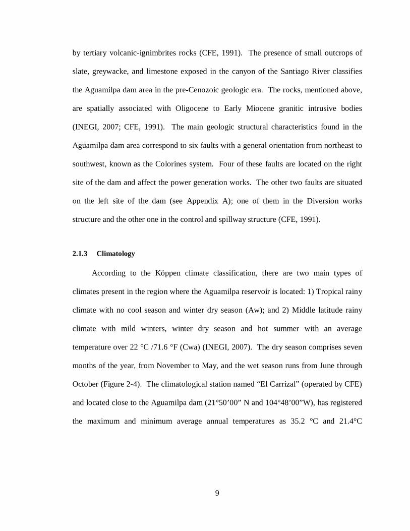
2.1.3 Climatology
According to the Köppen climate classification, there are two main types of
climates present in the region where the Aguamilpa reservoir is located: 1) Tropical rainy
climate with no cool season and winter dry season (Aw); and 2) Middle latitude rainy
climate with mild winters, winter dry season and hot summer with an average
temperature over 22 °C /71.6 °F (Cwa) (INEGI, 2007). The dry season comprises seven
months of the year, from November to May, and the wet season runs from June through
October (Figure 2-4). The climatological station named “El Carrizal” (operated by CFE)
and located close to the Aguamilpa dam (21°50’00” N and 104°48’00”W), has registered
the maximum and minimum average annual temperatures as 35.2 °C and 21.4°C

10
respectively, with an annual mean average temperature of 28.3°C. Moreover, this station
(ID=18045) has registered a total monthly mean precipitation of 1,155 mm per year, with
a total monthly mean evaporation of 2,086.5 mm per year, and a mean of 8.5 monthly
storms per year.
Figure 2-4: Types of Climates in Nayarit, Mexico (INEGI, 2007)
2.1.4 Power Generation
The Aguamilpa-Solidaridad hydroelectric project is one of twenty-seven projects
along the Santiago River that have been planned and developed by the Mexican

11
government to generate a hydro energetic potential of 4300 MW in Mexico. Marengo
(2006) reported that the Aguamilpa-Solidaridad dam contains an underground
hydroelectric power plant with three units of 320 MW of capacity each. Totaling 960
MW of installed power capacity, the Aguamilpa-Solidaridad dam ranks fourth in all of
Mexico (Table 2-1). Moreover, this hydroelectric plant has an annual average generation
rate of 2,131 GW*h and generates electricity for all of the states located in the
northwestern region of Mexico (CFE, 1991; ROP, 1997).
Table 2-1: Hydroelectric Dams with Most Power Capacity in Mexico
Name Power Capacity (MW)
Annual Average
Generation Rate (GW*h)
Height (meters)
Chicoasen 1500 2500 251
Malpaso 1080 2800 138
Infiernillo 1000 3160 149
Aguamilpa 960 2131 187
Angostura 900 2200 147
El Cajon 680 1496 186
Caracol 594 1480 126
Penitas 420 1910 53
Villita 300 1180 60
Zimapan 290 1292 200
Mazatepec 208 790 92
12
2.2 Water Quality Issues
As mentioned before the Santiago River is one of the two main inflows for the
Aguamilpa reservoir. Since middle of nineteen century, the construction of dams along
the Santiago River began with different purposes like power production, irrigation and
flow control. Nowadays, there are fifteen dams along the Santiago River in which the
Aguamilpa-Solidaridad Dam is included. There are two other similar large dams located
upstream of the Aguamilpa-Solidaridad Dam (Santa Rosa and El Cajon), and two
additional dams are planned and under construction (Arcediano and La Yesca) to meet
the energy demands. Three more dams (San Sebastian, Arroyo Hondo and San
Francisco) are planned to increase the storage capacity of the main cities located in the
central-northwest area of Mexico, Guadalajara, Leon and Tepic (Nelson et al.,
unpublished manuscript, 2008). The Santiago River has poor water quality due to non-
point wastewaters discharges from Guadalajara city metropolitan area, the excessive use
of fertilizers, and land use changes (de Anda et al., unpublished manuscript, 2007;
Barlow and Obregon, unpublished manuscript 2007). In addition, the current and
projected construction of dams along the Santiago River will potentially generate
environmental impacts that can affect the water quality of the river and the built
reservoir. Because, reservoirs can be used as indicators to examine the conditions of the
watershed, it is necessary to find tools that let Mexican authorities and researchers assess
the water quality conditions of the reservoirs that have been constructed along the
Santiago River. These tools can include water quality models which are being used to
better understand the degradation of water quality and the eutrophication of the
reservoirs.

13
2.3 Water Quality Models
A water quality model is a representation of the water quality processes that occur
in a particular studied waterbody. Water quality models and hydrodynamic models are
derived by applying the laws of conservation to conservative properties such as
momentum, heat energy, water mass, and contaminant mass. Water quality modeling
simulates the interaction between the sources of contamination and the water quality of a
given waterbody, known as cause-effect relationships. Based on how the cause-effect
relationships are implemented, Chapra, (1997); Martin and McCutcheon, (1999) classify
water quality models in two main categories:
1) Mechanistic. - Models that express their cause-effect relationships by using
mathematic formulas.
2) Empirical. - Models (or statistical models) that describe the cause-effect
relationships by using a minimum knowledge about how the studied system works.
In current practice, mechanistic models are used more than empirical models to
predict water movement and water quality, because they have the ability to incorporate
physical mechanisms that cause changes to the critical aquatic process. Further,
mechanistic water quality models have three important advantages over empirical models
that make them become more useful to test hypotheses about a particular waterbody,
diagnose water quality problems and predict the impact of various environmental
controls. The first advantage is that modeling allows water management experts to better
understand how the water quality of a waterbody behaves. The second advantage refers
to the calibration of the model that provides information about cause and effect
relationships and indicates what parts of the model have the most uncertainty. The third

14
advantage is the capability to predict responses, which the empirical models do not have
(Martin and McCutcheon, 1999). However, it is important to remember that all current
models still use empirical relationships to solve and understand complicated equations
that are involved in the process affecting water moment and water quality.
There are many water quality models available to simulate surface water flows
and water quality in rivers, lakes, estuaries, reservoirs or a combination of them. These
models can be classified as one, two or three-dimensional according to their capabilities
and limitations for simulating characteristics of a particular waterbody under study. Each
water quality model has its own characteristics, limitations and requirements, and its
selection depends on the studied waterbody and the goals that the modeler hopes to
achieve.
Due to the fact that the goal of this project is not to describe all the existing water
quality models, only the most common models that have been identified and used by the
United States Environmental Protection Agency (EPA) are described in this work. The
EPA (2007) defines in its website water quality models as tools for simulating the
movement of precipitation and pollutants from the ground surface through pipe and
channel networks, storage treatment units and finally to receiving waters. A brief
description of the water quality models recognized by the USEPA is included below.
2.3.1 AQUATOX
AQUATOX is a water quality model used to predict the fate of nutrients and
organic chemicals in waterbodies and their direct-indirect effects on the resident
organisms. AQUATOX is used to identify and understand the cause-effect relationships
between chemical water quality, physical environment, and aquatic life. Stratified lakes,

15
reservoirs, ponds, and rivers can be represented using this model. Some possible
applications of AQUATOX are: predicting effects of toxic substances on aquatic life,
determining effects of land use changes on aquatic life, and estimating time to recovery
of aquatic species after the contaminant loads are reduced. Its applicability has a range
from riverine systems to small ponds which are within the scale of stratified pond,
reservoir and lake ecosystems. AQUATOX assumes that the modeled waterbody is
uniformly mixed, except where stratification occurs in reservoirs and lakes (EPA, 2007).
Even though it is a one-dimensional model, AQUATOX can be a two-dimensional model
when it is linked to another water quality model (Nielsen, 2005; EPA, 2007).
2.3.2 EPDRiv1
EPDRiv1 is a system of programs used to perform one-dimensional (cross-
sectional) dynamic hydraulic and water quality simulations. The model was designed to
simulate dynamic conditions in rivers and streams, to analyze existing conditions,
perform waste load allocation, and allocate Total Maximum Daily Loads (TMDLs).
EPDRiv1 contains two computational components which are run separately. These
components are a hydrodynamic model EPDRiv1H and water quality model EPDRiv1Q.
This model may be used for modeling a one-dimensional waterbody with issues that do
not include metals, toxics or sediment transport (EPA, 2007).
2.3.3 WASP7
The Water Quality Analysis Simulation Program (WASP7) is a dynamic
compartment-modeling program used for simulating aquatic systems, including both the
water column and the underlying benthos. WASP7 is a water quality tool that helps users

16
interpret, predict water quality responses generated by natural phenomena and
anthropogenic pollution and formulate the best pollution control decisions (EPA, 2007;
Hellyer, 2008). This model lets the user simulate one, two and three-dimensional
systems, and different types of contaminants. Moreover, WASP can provide flows,
depths, velocities, temperature, salinity and sediment fluxes when it is linked with
hydrodynamic and sediment transport models.
2.3.4 QUAL2K
QUAL2K is a one-dimensional river and stream water quality model that assumes
the channel is well-mixed vertically and laterally. This model represents a modernized
version of the QUAL2E model (Brown and Barnwell, 1987). The QUAL2E model has
been widely used by the USEPA and other global environmental agencies for modeling
the water quality of rivers and channels (Salvai and Bezdan, 2008). In addition to the
well known features of QUAL2E, the new QUAL2K contains new features such as
model segmentation, carbonaceous Biochemical Oxygen Demand (cBOD) speciation,
anoxia and denitrification, sediment-water interactions, bottom algae, light extinction,
pH, and pathogens.
2.3.5 CE-QUAL-W2
Originally developed in 1975 by the U.S. Army Corps of Engineer (USACE)
Waterways Experiment Station (WES), “CE-QUAL-W2 is a two-dimensional, laterally
averaged, hydrodynamic and water quality model. Because the model assumes lateral
homogeneity, it is best suited for relatively long and narrow waterbodies exhibiting
longitudinal and vertical water quality gradients.” (Cole and Wells, 2003) The definition

17
given above can be explained in two parts. First, the term two-dimensional means that
two of the three dimensions of the model are represented by a series of cells for which
governing equations can be solved. The second part “laterally averaged,” means that the
two dimensions of CE-QUAL-W2 look for the longitudinal (reservoir length) and vertical
(reservoir depth) dimensions of the studied waterbody. Yet, this model (called W2) was
developed for reservoirs and narrow, stratified estuaries and it is efficient and cost-
effective use in comparison with other two-dimensional models. CE-QUAL-W2 has
been improved for the last three decades and it was originally known as LARM (Laterally
Averaged Reservoir Model) developed by Edinger and Buchak in 1975 (Nielsen, 2005).
LARM, renamed CE-QUAL-W2 Version 1.0 in 1986 for the addition of water quality
algorithms, is a modification of the Laterally Averaged Estuary Model (LAEM) and later
Generalized Longitudinal-Vertical Hydrodynamics and Transport (GLVHT) model
(Martin and McCutcheon, 1999).
2.4 Model Selection
The increasing demand of water supply and overexploiting groundwater in the
biggest cities in Mexico have made the Government search for new alternatives to supply
potable water (Comision Nacional del Agua [CONAGUA], 2008). These new sources
may be the surface waters which comprise rivers, lakes and reservoirs. However, the
water quality of Mexican surface waters present high levels of pollution which make
them unusable for human consumption. This is why the National Water Commission of
Mexico (CONAGUA) and water management officials want to know the levels of
eutrophication in the national waterbodies and what practices can be incorporated to
18
improve their water quality. As described earlier, water quality models have been used
for years as tools to interpret, predict and better understand the water quality changes,
eutrophication and hydrodynamics in rivers, lakes, estuaries, reservoirs or a combination
of them. In most of the cases, these models have been used to successfully simulate
temperate waterbodies. After reviewing literature and understanding the characteristics
of the Aguamilpa reservoir, the CE-QUAL-W2 model was chosen to simulate the water
quality of the reservoir. CE-QUAL-W2 is a two-dimensional laterally-averaged
hydrodynamic and water quality model that has been applied frequently to long-narrow
reservoirs and estuaries (Cole and Wells, 2003). This model was selected not only
because the Aguamilpa reservoir is characterized as long and narrow, but also based on
the results of previous studies (Nielsen, 2005; Williams, 2008; de Victoria, 1996) that
exhibit reservoir circulation and significant longitudinal and vertical variations in water
quality and productivity. Since its creation, CE-QUAL-W2 has been improved by
including new codes and algorithms. As a result of these improvements, different
versions of CE-QUAL-W2 have been released in the market and they will be explained
together to their capabilities and limitations as follows.
2.4.1 CE-QUAL-W2 Versions
Every released version of CE-QUAL-W2 has included changes which have
improved the model. By the time this project was finished, the CE-QUAL-W2 version
3.6 became the newest version of the model but it has not been released yet. Previous
versions of the model comprise:

19
• CE-QUAL-W2 v 3.5. - This is the current model release which includes
capabilities to simulate zooplankton and macrophyte (Portland State
University [PSU], 2008).
• CE-QUAL-W2 v 3.2. - Version 3.2 presented improvements such as the
addition of a new algorithm which estimates suspended solids
resuspension due to wind-wave action.
• CE-QUAL-W2 v 3.1 and v 3.0. - Numerical solution scheme and water
quality algorithms were added to these versions which included algal
groups and epiphyton/peripyton groups.
• CE-QUAL-W2 v 2.0. - In this version, the mathematical description of
the prototype and the computational accuracy and efficiency of the model
were improved (Cole and Wells, 2003).
The version used for this study is CE-QUAL-W2 v 3.2 which is the latest
supported code from the USACE. Moreover, the executable named
w2_32agpm_tvd_weir.exe has been modified to work with AGPM pre and post
processors.
2.4.2 CE-QUAL-W2 Capabilities and Limitations
As mentioned in Section 2.3 (Model selection), specific criteria were used to
select the most suitable model for this study. An important part of the selection process
was reviewing the CE-QUAL-W2 capabilities and limitations in order to understand its
application to the Aguamilpa reservoir. As with every other computational model, CE-
QUAL-W2 has distinct capabilities and limitations in its application. The model has the

20
ability to predict water surface elevations, velocities, temperatures, several water quality
constituents and over sixty derived water quality variables. Waterbodies, which present a
complex geometric shape, can be represented by using a finite difference computational
grid. Most of the inflows and outflows of the waterbody are represented as precipitation,
point/nonpoint sources, upstream/downstream branches, and other methods. Moreover,
W2 is useful for long term simulations and water quality responses to different
meteorological scenarios which are important points for this study.
The limitations of CE-QUAL-W2 are that the governing equations are laterally
and layer averaged. In other words, lateral averaging assumes that lateral variations in
velocities, temperatures, and constituents are not considered. This assumption may not
be appropriate for large waterbodies showing significant lateral variations in water
quality (Cole and Wells, 2003). The model may not provide accurate results where there
is significant vertical acceleration because an algorithm for vertical momentum is not
included. Also several water quality processes are not simulated such as dynamic
sediment oxygen demand, sediment transport and accumulation, and toxics. The model
does not simulate zooplankton and their effects on phytoplankton or recycling of
nutrients. Macrophytes effects are not included either in the hydrodynamics and water
quality parts of the model. In addition to these limitations, the model is also complicated
and time consuming, requiring knowledge of hydrodynamics, aquatic biology, aquatic
chemistry, numerical methods, programming, and statistics. However, improvements to
the model are being continuously developed in order to decrease the limitations of the
model. For more information about capabilities and limitations of the CE-QUAL-W2
version 3.2 can be found in the User Manual (Cole and Wells, 2003).
21
2.5 Subtropical Reservoirs
The degree to which lakes and reservoirs are affected by pollution depends on
whether they are deep or shallow, large or small, and tropical/subtropical or temperate
(Hutchinson, 1957). Subtropical reservoirs have not been studied as much as temperate
reservoirs, because they are located in developing countries where there is not enough
technology that allows studying this type of reservoirs. Mexican reservoirs are classified
as subtropical due to their geographical location. The Aguamilpa reservoir is classified
as subtropical according to the climatological characteristics of the region. Man-made
lakes or reservoirs located in subtropical areas present more complex thermodynamic,
biologic and hydrologic characteristics than reservoirs located in temperate areas. This
is because subtropical reservoirs are relatively abundant as compared with temperate
reservoirs, and they also present higher temperatures that accelerate the biological and
chemical processes occurring in them (Ayres et al., 1997). In general, subtropical
reservoirs are less able to assimilate nutrients which accelerate eutrophication as nutrient
loads are increased. Stratification and eutrophication processes in subtropical reservoir
are described as follows.
2.5.1 Stratification
The most important and dominant physical process in a reservoir, is its thermal
stratification which is the result from heating the water by the sun. This thermal process
regulates the rates of chemical reactions and biological process. Thermal stratification
occurs when the density of the upper water’s reservoir is decreased by heating, and the
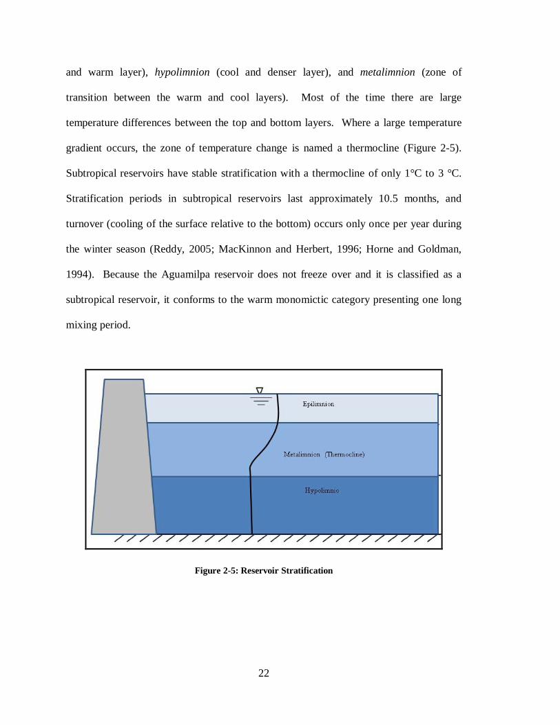
water is subjected to wind, resulting in three main layers known as: epilimnion (upper
22
and warm layer), hypolimnion (cool and denser layer), and metalimnion (zone of
transition between the warm and cool layers). Most of the time there are large
temperature differences between the top and bottom layers. Where a large temperature
gradient occurs, the zone of temperature change is named a thermocline (Figure 2-5).
Subtropical reservoirs have stable stratification with a thermocline of only 1°C to 3 °C.
Stratification periods in subtropical reservoirs last approximately 10.5 months, and
turnover (cooling of the surface relative to the bottom) occurs only once per year during
the winter season (Reddy, 2005; MacKinnon and Herbert, 1996; Horne and Goldman,
1994). Because the Aguamilpa reservoir does not freeze over and it is classified as a
subtropical reservoir, it conforms to the warm monomictic category presenting one long
mixing period.
Figure 2-5: Reservoir Stratification
23
2.5.2 Eutrophication
The quantity of nutrients found in a reservoir in addition to the environmental
factors such as temperature and light soluble gases in relation to the amount of reservoir
phytoplankton defines its trophic level. Ortiz et al., 2006 describes the trophic state as
the quantity of organic matter in aquatic ecosystems, and this trophic state is used as an
indicator of the pollution level in a reservoir. The concentration of nutrients
(phosphorous and nitrogen) and chlorophyll α as well as transparency are used to classify
a waterbody’s trophic state. Depending on the reservoir’s trophic state, the studied
reservoir is classified as oligrotrophic, mesotrophic or eutrophic.
• Oligotrophic reservoirs: They are generally deep with low nutrient levels
and clear blue water.
• Mesotrophic reservoirs: These reservoirs present intermediate nutrient
levels between oligotrophic and eutrophic conditions.
• Eutrophic reservoirs: High nutrients and rates of primary productivity
(net photosynthesis) are primary characteristics of eutrophic reservoirs.
The presence of surface blooms of blue-green algae is a typical.
However, subtropical reservoirs can be eutrophic when nutrient concentrations are
low, due to the high water temperatures. Problems with eutrophication occur frequently
for subtropical reservoirs, particularly those recently constructed. For instance, Lake
Volta (Ghana), Lake Kariba (Zimbabwe) and Lake Brokopondo (Surinam) (Reddy, 2005)
all fit this category. It is important to remember that the most common primary limiting
nutrient in subtropical reservoirs may be the nitrogen produced by denitrification. This
denitrification is generated by the anoxic conditions in the hypolimnion and bottom

24
sediments which occur with high frequency in deep-subtropical reservoirs. These
conditions and the better relationship observed between chlorophyll α-nitrogen than
chlorophyll α-phosphorus suggests nitrogen as the primary limiting nutrient for
subtropical reservoirs (Huszar et al., 2006; Lewis, 2002; Mazumder and Havens, 1998).

25
3 Model Development
In this part, a description of the CE-QUAL-W2 model development for the
Aguamilpa reservoir is presented. It is important to mention that due to the availability of
data, the 1995 and 1996 years were chosen to develop the initial model. However, the
process for developing the model would be the same for any period of record that
adequate data can be obtained. The following sections of this chapter discuss the model
input files including bathymetry, boundary and initial conditions, and the associated
assumptions for their creation. Depth, length, width and other physical characteristics of
the reservoir are represented by its bathymetry which is described in the bathymetry
section (Section 3.1). The description of the control file which manages requisite files is
given in the initial conditions section (Section 3.2). The meteorological file section
(Section 3.3) describes the climatological data used and where they can be obtained. The
boundary conditions section (Section 3.4) consists of a description of how inflow,
outflow, and inflow temperatures files were created as well as their use.
3.1 Bathymetry
The development of the CE-QUAL-W2 model began by creating the reservoir’s
bathymetry data. Bathymetry includes the depth, width, length, orientation and storage
capacity of the reservoir. Getting a high-quality bathymetry of the reservoir is important

26
to create an accurate model. The bathymetry of the Aguamilpa reservoir was created by
using 1:50000 scale Digital Elevation Models (DEMs) obtained from The National
Institute of Statistic, the Geography and Information Technology of Mexico (INEGI) and
the Watershed Modeling System version 8.0 (WMS) software (Nelson, 2006). The codes
of the necessary DEMs to cover the Aguamilpa reservoir are: F13D11, F13D12, F13D13,
F13D21, F13D22, F13D23, F13D31, F13D32 and F13D33 (INEGI, 2008). WMS, which
processes the DEM data to produce a CE-QUAL-W2 bathymetry file was developed by
the Environmental Modeling Research Laboratory (EMRL) which is part of the Civil and
Environmental Engineering Department at Brigham Young University. Presently WMS
is maintained by Aquaveo LLC. WMS is defined by Aquaveo (2008) as “a
comprehensive graphical modeling environment for all phases of watershed hydrology
and hydraulics.” WMS provides a variety of capabilities which include cross-section
extraction from terrain data, watershed delineation, calculation of the geometry watershed
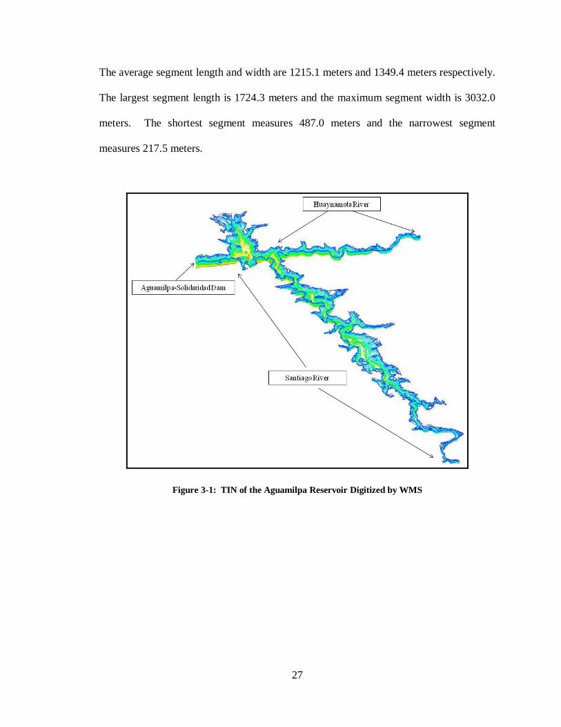
and others. DEMs were converted to Triangulated Irregular Networks (TINs) using
WMS to define the boundaries and storage capacity of the Aguamilpa reservoir (Figure
3-1). The reservoir’s boundaries were set at a maximum elevation of 232 meters
(corresponding to the high-water level in the reservoir), resulting in an extension of the
reservoir approximately 60 Km along the Santiago River and 25 Km along the
Huaynamota River.
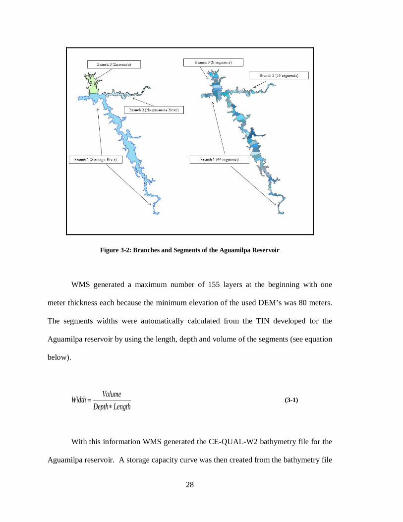
The bathymetry of the Aguamilpa reservoir CE-QUAL-W2 model includes a total
of 3 branches and 74 segments. The three created branches are identified as: Branch 1
(Santiago River), Branch 2 (Huaynamota River) and Branch 3 (Ensenada or ungauged
branch) with Branch 1 being the largest and Branch 3 the shortest (Figure 3-2).
27
The average segment length and width are 1215.1 meters and 1349.4 meters respectively.
The largest segment length is 1724.3 meters and the maximum segment width is 3032.0
meters. The shortest segment measures 487.0 meters and the narrowest segment
measures 217.5 meters.
Figure 3-1: TIN of the Aguamilpa Reservoir Digitized by WMS
28
Figure 3-2: Branches and Segments of the Aguamilpa Reservoir
WMS generated a maximum number of 155 layers at the beginning with one
meter thickness each because the minimum elevation of the used DEM’s was 80 meters.
The segments widths were automatically calculated from the TIN developed for the
Aguamilpa reservoir by using the length, depth and volume of the segments (see equation
below).
LengthDepthVolumeWidth
∗= (3-1)
With this information WMS generated the CE-QUAL-W2 bathymetry file for the
Aguamilpa reservoir. A storage capacity curve was then created from the bathymetry file

29
and compared with the field data obtained from CFE and GRUBA to check the accuracy
of the bathymetry data. As shown in Figure 3-3, the created storage capacity curve is
similar to the observed proving the accuracy of the bathymetry file of the Aguamilpa
reservoir. This comparison showed that the DEM 1:50,000 available from INEGI (2008)
is adequate to develop an accurate bathymetry for the Aguamilpa reservoir. The storage
capacity curves created for the branches and segments are shown in Appendix A. These
storage capacity curves show the storage of the reservoir at different elevations and
locations.
Figure 3-3: WMS Total Storage Capacity Curve vs. Field Data
However, 13 more layers were added by hand to the 155 generated layers (1
meter) to obtain 168 layers of a maximum number for each single segment. This is
because the maximum reservoir’s depth is 187 meters (613.5 feet) not 155 meters (508.5
feet). Besides, a bathymetry made by GRUBA S.A. de C.V. [GRUBA] (1997) reported

30
the minimum elevation of the reservoir at 64.3 meters (211.0 feet) with a volume of 0.001
Hm3 (0.81 acre-feet).
A pre-processor named W2i, included in the W2i-AGPM Modeling System UI for
CE-QUAL-W2 v3.2 software, is a powerful water quality modeling tool created and
managed by Loginetics, Inc (Loginetics, 2008). W2i was used in several occasions for
developing this study. One of its uses was to view the created bathymetry of the
Aguamilpa reservoir. Viewing the bathymetry in W2i pre-processor allowed an
improvement in the bathymetry created by WMS. The minimum layer width in the
bathymetry file was limited to 10 meters to increase model stability and decrease model
run times. The final bathymetry grid of the branch 1 (Santiago River) is presented in
Figure 3-4, and the final bathymetry grids of branch 2 and branch 3 are shown in
Appendix A.
Figure 3-4: W2 Bathymetry Grid of Branch 1 (Santiago River)
31
3.2 Initial Conditions
Initial conditions were specified in the control file which manages all the other
required files. Number of waterbodies (1), number of branches (3) and segments (74),
bottom elevation of the reservoir (64.30 meters), elevation of the spillway (210 meters)
and power generation releases elevation (180 meters) are the initial conditions specified
for the Aguamilpa reservoir model. These initial conditions were input in the control file
shown in Appendix C.
In addition to these initial conditions, water surface elevations were required for
each computational segment and layer before starting the model simulation. The model
simulation was set to begin on January 1, 1995 and finish on December 31, 1996. These
dates were converted to Julian Days (JDAYS) which is format required for the CE-
QUAL-W2 model for all the input files. These years were selected because their data
were the most complete available to develop the required files of the CE-QUAL-W2
model for the Aguamilpa reservoir. The initial water surface elevation on January 1,
1995, was set at 218.32 meters or 716.3 feet (above sea level) and it was measured at the
Aguamilpa-Solidaridad dam site of the Aguamilpa reservoir. The observed daily water
surface elevations data for the modeling years were obtained from a water quality study
prepared by GRUBA (1997). These daily average water surface elevations data were
used to create an observed elevation file used for the water balance calibration of the
model, which will be described on section 4.1.

32
3.3 Meteorological File
The meteorological file of the Aguamilpa reservoir includes hourly data of air
temperature, dew point temperature, wind speed, wind direction, and cloud cover. Air
temperatures and dew point temperatures were input in the model in degrees Celsius,
wind speed in meters per second, wind direction values were converted from degrees to
radians, and cloud cover assigned values between 0 and 10. Data from ten climatological
stations, located around the Aguamilpa reservoir and managed by the State of Nayarit and
CFE, were obtained. However, these stations were not used because the meteorological
data gathered from them only had daily average temperature and in some cases the data
were incomplete. However, the climatological station located at the Tepic airport
(NOAA, 2008), gathered hourly climatological data it was chosen to create the
meteorological file. Modifications and assumptions (described in section 3.5.1) were
made to the Tepic climatological data in order to represent the meteorological conditions
at the Aguamilpa reservoir. The W2i-AGPM utility helped identify that the Tepic airport
station was the closest climatological station that included hourly data. This was found
by using the “Find Met” option. The climatological data of the Tepic airport was
downloaded from the National Oceanic and Atmospheric Administration (NOAA)
International Data Centers, and the general information of this station is described on the
following Table 3-1.

33
Table 3-1: Climatological Station Information
Station Information
Name: Tepic airport ID: 765560 Dates of data: 1995 – 1996 (hourly) Location: ~ 31 kilometers (19.262 miles) from the Aguamilpa reservoir
• 21°31'1.20"N • 104°52'58.80"W
3.4 Boundary Conditions
In order to run the CE-QUAL-W2 model for the Aguamilpa reservoir, the
following boundary conditions files were required: inflows, outflows, inflow
temperatures, inflow constituents and distributed tributaries inflows. These boundary
conditions were important for the model to represent the behavior of the reservoir. The
development of the required boundary conditions files are described in this section and
the adjustments made for these files are presented in section 3.5.2
3.4.1 Inflows
There are approximately nine gauging stations useful for defining the boundary
conditions that are located on the three main branches of the Aguamilpa reservoir
(Santiago, Huaynamota and Ensenada). These gauging stations, shown in Figure 3-5, are
La Playa, Cerro Blanco, El Capomal, Despeñadero, Huaynamota, Chapalagana, Jesús
María, Paso de la Yesca and El Caiman. The National Power Commission (CFE) or the
National Water Commission (CONAGUA) operates the gauging stations. Data from
these gauging stations were provided by CIATEJ and CFE Mexico City. The La Playa

34
and Cerro Blanco gauging stations were used to create the inflow file for branch 1
(Santiago). Inflow files for branch 2 (Huaynamota) and branch 3 (Ensenada) were
estimated by using water velocities and are described in section 3.5.2. The other gauging
stations were not used to create the inflow files for branches 2 and 3 because they were
not operational, or the data were incomplete for the period being modeled.
Figure 3-5: Location of Gauging Stations
3.4.2 Outflows
The outflow boundary conditions were defined from the discharge records taken
at the Aguamilpa-Solidaridad Dam from 1995 to 1996. Hourly outflow data were
gathered from the water quality study prepared by GRUBA (1997). However, these data
only included water releases used to generate energy, and did not include other outflows
from the reservoir, such as the minimum ecological flows and irrigation intakes. These

35
data were the only hourly outflow data available at the time this work was concluded.
After the outflow data were analyzed, it was observed that most of the hourly water
releases for power generation from the dam occur between 7:00 PM and 10:00 PM local
time at night, being this period of time the daily peak power generation (Alvaro Perez,
phone communication, September 30, 2008).
3.4.3 Inflow Temperatures
Upstream inflow temperature data for the Aguamilpa’s branches were not
available. These data had to be estimated by using daily average air temperature from
climatological stations, located close to the inflow of the three branches, and by making
the assumptions which will be discussed in section 3.5.2. There were 3 climatological
stations used:
• Paso la Yesca and Cerro Blanco for branch 1 (Santiago River)
• Jesús María and Chapalagana for branch 2 (Huaynamota River)
• Capomal and Carrizal for branch 3 (Ensenada River)
The daily average temperature data from the climatological stations mentioned
above were gathered from CFE and CONAGUA. The unrecorded inflow temperatures
data is the primary weakness of the developed model, and it is important to include these
data in future monitoring programs to create more accurate models.
3.4.4 Inflow Constituents
The inflow constituent files for the main branches of the Aguamilpa reservoir
could not be created by using water quality data from the reservoir. This is because there
were no water quality data available or the data were not sufficient to be used for

36
simulation. Due to the lack of water quality data, the initial model development for the
Aguamilpa reservoir was focused on water temperature. However, in order to
demonstrate the possibility and utility of simulating water quality parameters, some data
from a separate reservoir were used. While the data are useful as a demonstration, they
should not be used to infer specific results, but rather to develop appropriate guidelines
for future monitoring. These example water quality simulations will be shown and
described in section 4.3.
3.4.5 Distributed Tributary Files
Distributed tributary inflows are used to develop nonpoint source loadings
adjacent to the branches along the length of the reservoir. The distributed tributary
option provides the user with means to account for contributions that are not included as
inflows to the reservoir. These unaccounted sources generally represent smaller,
ungauged tributaries, precipitation on the lake, groundwater inflows and wastewater
discharges. This option distributes inflows into every branch segment weighted by the
segment surface area (Cole and Wells, 2003). Three different types of distributed
tributary files were created inflow, inflow temperature and inflow concentration for each
branch of the Aguamilpa reservoir. The distributed tributary inflow files contained the
values calculated from the water balance which is described in section 4.1. As explained
in section 3.4.3, the inflow temperature data had to be estimated and their monthly
average values were used as source of data to create the distributed tributary inflow
temperature files.

37
3.5 Data Gaps
As mentioned in previous sections, the best available data were used to create the
input files for developing the CE-QUAL-W2 model of the Aguamilpa reservoir. Several
gaps were identified made in the input data in order to get a more accurate model. The
data gaps, along with the assumptions made to complete the setup of the initial model for
the Aguamilpa reservoir are discussed in the following sections.
3.5.1 Meteorological Adjustments
The hourly climatological data, obtained from the Tepic airport station were
modified before being used to create the meteorological file of the Aguamilpa reservoir.
Adjustments on the climatological data were necessary because the Aguamilpa reservoir
is located at an elevation of 240 meters (787.4 ft) and the Tepic airport climatological
station is at 915 meters (3000 ft) above sea level. This difference in elevation produces
variability on weather conditions that affect the mixing and thermal effects on the
Aguamilpa reservoir. For instance, wind speed will generally be higher and air
temperature colder at the higher elevation Tepic station than the reservoir. The
modifications to the meteorological file began by adjusting time. The downloaded data
uses Greenwich Mean Time (GMT) and the model required the local time in Aguamilpa,
which is seven hours less than the GMT during standard time and six hours less than
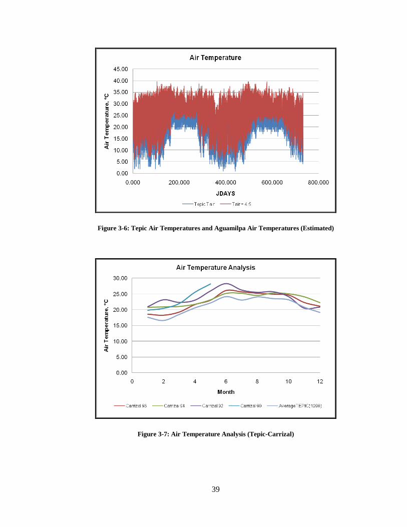
GMT during daylight saving time (Holiday-Weather, 2008). As shown on Figure 3-6,
4.5 degrees Celsius (°C) were added to the air temperature gathered from the Tepic
airport station in order to be more representative of air temperature at the Aguamilpa
reservoir. An adjustment of 4.5 °C was chosen after an air temperature comparison
38
analysis was performed. This analysis included comparing historical average air
temperature data of the Tepic and El Carrizal climatological stations located at Tepic and
the Aguamilpa-Solidaridad Dam respectively (Figure 3-7). It is important to remember
that the climatological data gathered from the El Carrizal station was not complete and it
was only average daily data. Also, the dew point temperatures were adjusted for
conditions at the Aguamilpa reservoir. They were calculated by using the calculated air
temperatures at Aguamilpa and estimating the percentage of relative humidity, which was
calculated with equation below (Wanielista et al., 1997).
AIRAIRD TTfT 1.0112)9.0112(81
+−+= (3-2)
where:
f = Percentage Relative humidity, frictionless
TAIR = Air Temperature, °C
TD = Dew Point Temperature, °C
Other meteorological data such as wind speed, wind direction, and cloud cover
from the original meteorological file were not modified because they were assumed to be
the same at the Aguamilpa reservoir. This assumption reveals an important need to
collect the data locally at that dam for the final model, because these factors produce
effects on thermal conditions and mixing processes occurring in the reservoir.
39
Figure 3-6: Tepic Air Temperatures and Aguamilpa Air Temperatures (Estimated)
Figure 3-7: Air Temperature Analysis (Tepic-Carrizal)
40
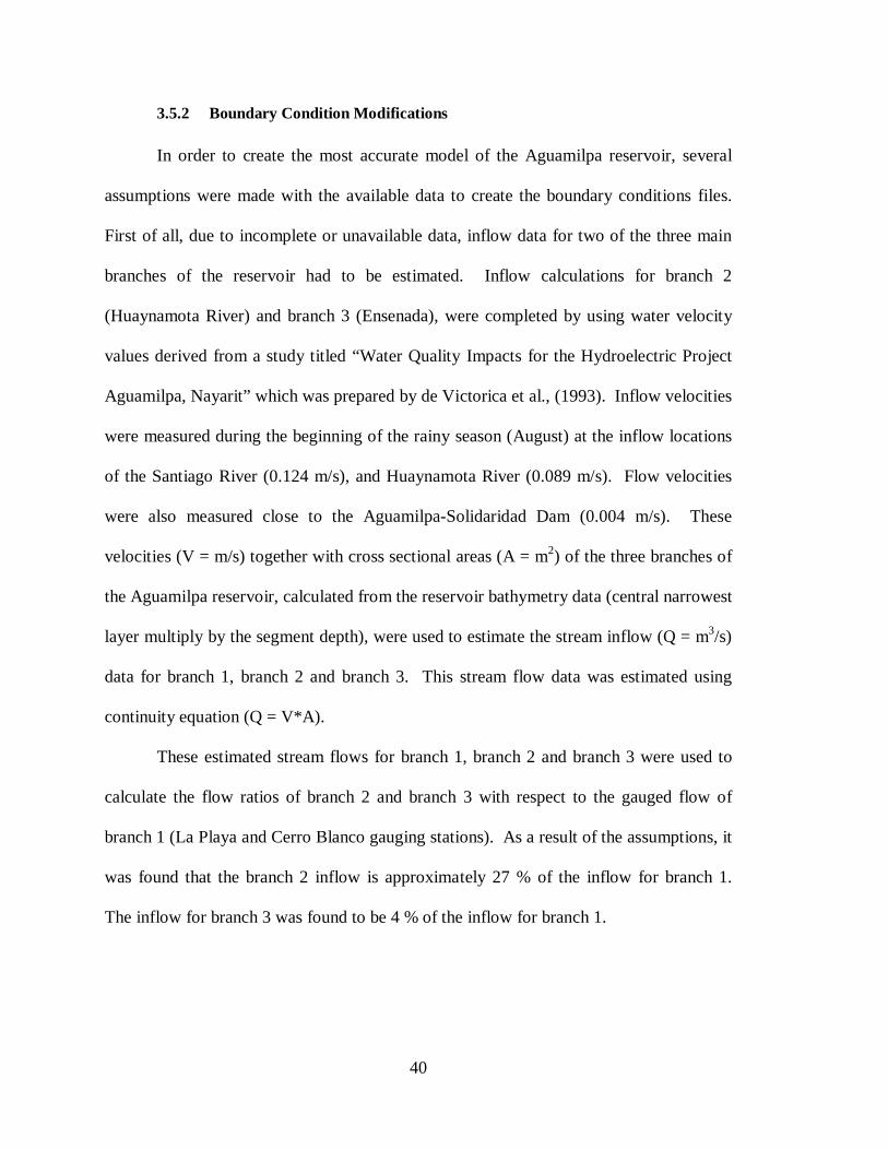
3.5.2 Boundary Condition Modifications
In order to create the most accurate model of the Aguamilpa reservoir, several
assumptions were made with the available data to create the boundary conditions files.
First of all, due to incomplete or unavailable data, inflow data for two of the three main
branches of the reservoir had to be estimated. Inflow calculations for branch 2
(Huaynamota River) and branch 3 (Ensenada), were completed by using water velocity
values derived from a study titled “Water Quality Impacts for the Hydroelectric Project
Aguamilpa, Nayarit” which was prepared by de Victorica et al., (1993). Inflow velocities
were measured during the beginning of the rainy season (August) at the inflow locations
of the Santiago River (0.124 m/s), and Huaynamota River (0.089 m/s). Flow velocities
were also measured close to the Aguamilpa-Solidaridad Dam (0.004 m/s). These
velocities (V = m/s) together with cross sectional areas (A = m2) of the three branches of
the Aguamilpa reservoir, calculated from the reservoir bathymetry data (central narrowest
layer multiply by the segment depth), were used to estimate the stream inflow (Q = m3/s)
data for branch 1, branch 2 and branch 3. This stream flow data was estimated using
continuity equation (Q = V*A).
These estimated stream flows for branch 1, branch 2 and branch 3 were used to
calculate the flow ratios of branch 2 and branch 3 with respect to the gauged flow of
branch 1 (La Playa and Cerro Blanco gauging stations). As a result of the assumptions, it
was found that the branch 2 inflow is approximately 27 % of the inflow for branch 1.
The inflow for branch 3 was found to be 4 % of the inflow for branch 1.

41
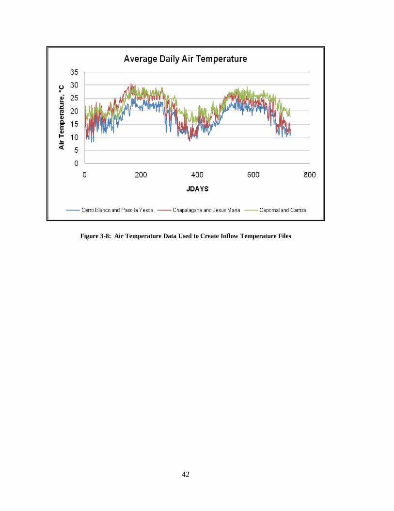
Similar to the inflow, assumptions were used to develop the inflow temperature
files and the distributed tributary inflow temperature files as well. There were no inflow
temperature data available that could be used for the CE-QUAL-W2 model for the
Aguamilpa reservoir. For the purposes of developing an initial model air temperature
data from climatological stations, described in section 3.4.3, were used as the basis for
the inflow temperature files and the distributed tributary inflow temperature files (Figure
3-8). Air temperatures were increased 5 °C to better represent the water temperatures in
the inflow branches of the reservoir. The 5 °C value was chosen after running several
thermal simulations and comparing them with field data reported by GRUBA (1997) and
the current readings that are being monitored by CIATEJ (section 4.2). As mentioned
before this estimation is one of the primary weaknesses of the model and recording daily
water inflow temperatures are essential to develop a more accurate model. The
distributed tributary inflow temperature files were created by using the average monthly
estimated inflow temperature data for the three branches of the Aguamilpa reservoir.
Since the distributed tributary inflow files were created from the results obtained
in the water balance, which is described in section 4.1, their assumptions are described in
the same section. The assumptions made for the inflow constituents files and distributed
inflow constituents files, are described in section 4.3.
42
Figure 3-8: Air Temperature Data Used to Create Inflow Temperature Files

43
4 Results
In this section, results of the water balance calibration, temperature simulations,
and example water quality simulations for the Aguamilpa reservoir are presented. The
data preparation required to develop the model has been presented in the previous
chapters. The process of creating a CE-QUAL-W2 water quality model for the
Aguamilpa reservoir with both a thermal and example water quality simulation identified
the available sources for information as well as the design of a monitoring and data
acquisition plan to obtain the minimum required data. The monitoring and data
acquisition plan is also explained in this section.
4.1 Water Balance Calibration
The first step in the Aguamilpa water quality simulation was to perform a water
balance. An accurate accounting of the water budget for a reservoir is essential for a
simulation and the calibration of the model. All the recorded and estimated inflow and
outflows data (described in sections 3.4 and 3.5.2) for 1995 and 1996 were used to
establish the water balance of the Aguamilpa reservoir. As shown in Figure 4-1, the
reservoir’s water budget was checked by comparing predicted elevations with observed
elevations. This comparison was formulated by using the CE-QUAL-W2 V3.2 and the
water balance tools that generate the inflows needed to establish an accurate water

44
balance (Figure 4-2). The water surface elevation differences were converted to daily
volumes which were positive or negative.
Figure 4-1: Observed and Modeled Water Surface Elevations Comparison
Figure 4-2: Water Balance Calibration of the Aguamilpa Reservoir

45
The volume differences were added to the inflows of the model through the three
distributed tributary inflows files, which represent all the ungauged inflows and outflows
for the Aguamilpa reservoir (ecological flow, irrigation intakes, precipitation,
evaporation, seepage, bank storage and ungauged tributaries inflows). These three
distributed tributary inflow files were estimated from the inflows and outflows generated
in the water balance. The maximum difference between the observed and modeled water
surface elevations was approximately 12.5 %, meaning that most of the distributed
tributary inflows may correspond to the ungauged tributaries inflows. However, large
negative flow values were obtained for some days of simulation, meaning that there could
be some water releases from the reservoir that were not taken into account (evaporation,
irrigation intakes, and ecological flows). In order to decrease the large negative values, a
five-day average inflow calculation was performed to reduce the error generated by the
ungauged outflows of the Aguamilpa reservoir. This five-day inflow calculation was
randomly chosen trying to distribute the error throughout a week. Because this average
reduced the large negative values, it was not necessary to try other average days. The
allocation of the error in simulated versus measured volumes to the distributed tributary
inflow through the three main branches of the reservoir used the following criteria: The
distributed tributary inflows for branch 3 and branch 2 were estimated to be 4 % and 27
% respectively of the inflows contributing to the water balance. The distributed tributary
inflows for branch 1 were estimated by subtracting the sum of the distributed tributary
inflow estimated for branch 1 and branch 2 from the total distributed tributary inflows
generated in the water balance.

46
4.2 Thermal Simulation
As mentioned in section 2.5.1 the mixing regime in deep subtropical reservoirs is
warm monomictic, meaning that the reservoir only turns over once per year (during
winter season). These high temperatures in the subtropical reservoirs accelerate the rates
of chemical reactions and biological processes. The thermal simulations run for the
Aguamilpa reservoir proved that CE-QUAL-W2 is suitable for deep subtropical
reservoirs. Insufficiency of In-Situ water temperature data and inflow water temperature
prohibits an accurate thermal calibration for the Aguamilpa reservoir. However, making
some assumptions such as increasing the wind sheltering coefficient (1.45), wind
function coefficients, solar radiation shading (0.85) and increasing/decreasing the
estimated inflow temperatures, allow the simulation of similar thermal conditions that
have been recorded by CIATEJ in the Aguamilpa reservoir (Figure 4-3).
The wind sheltering coefficient has the most effect on temperature during
calibration and it is necessary to adjust it before changing any other coefficient.
According to Cole and Wells (2003), previous applications varied the wind sheltering
coefficients have found that values from 0.5-0.9 are used for reservoirs located at
mountainous and/or dense vegetative canopy areas. Values of 1.0 are used for open
terrain areas and values over 1 should be used for funneling effects on systems with steep
banks, like Aguamilpa reservoir’s area in which, after several runs, a value of 1.45 was
chosen. The wind function coefficients have effects in the surface heat exchange and
evaporation of the reservoir.
47
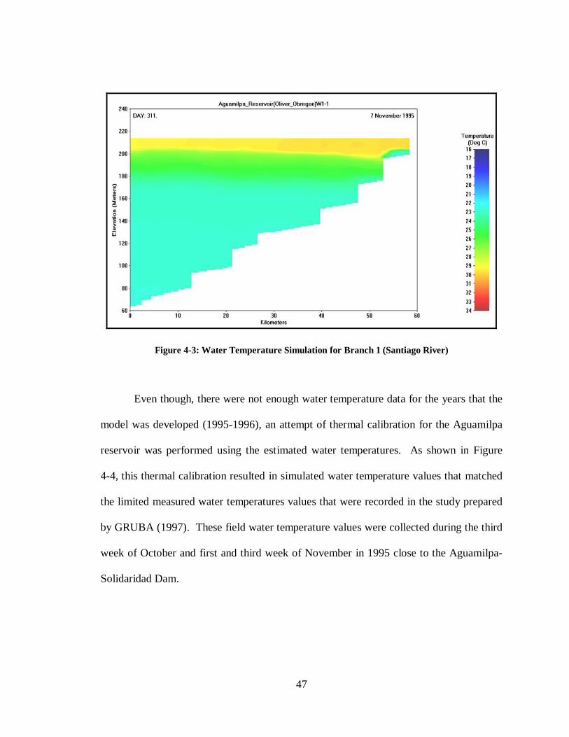
Figure 4-3: Water Temperature Simulation for Branch 1 (Santiago River)
Even though, there were not enough water temperature data for the years that the
model was developed (1995-1996), an attempt of thermal calibration for the Aguamilpa
reservoir was performed using the estimated water temperatures. As shown in Figure
4-4, this thermal calibration resulted in simulated water temperature values that matched
the limited measured water temperatures values that were recorded in the study prepared
by GRUBA (1997). These field water temperature values were collected during the third
week of October and first and third week of November in 1995 close to the Aguamilpa-
Solidaridad Dam.

48
Figure 4-4: Field vs. Modeled Water Temperature Data (1995)
4.3 Example Water Quality Simulations
As explained in section 3.4.4, there were not enough available water quality data
from the three main branches of the Aguamilpa reservoir to run constituent simulations.
Nevertheless, to demonstrate how a CE-QUAL-W2 water quality model for the
Aguamilpa reservoir may work, water quality simulations were run using input data from
a different reservoir.
The water quality input data used to create the inflow constituents files and the
distributed tributary inflow concentration files were gathered from the East Canyon
reservoir located in the state of Utah, in the western United States. It is important to
mention that the Aguamilpa reservoir and East Canyon reservoir are not similar in
characteristics. The example water quality simulations included twenty water quality

49
parameters, such as total dissolved solids (TDS), dissolved oxygen (DO), inorganic
suspended solids group 1 (ISS1), dissolved silica (DSI), dissolved inorganic phosphorous
(PO4), ammonium (NH4), nitrate-nitrite (NO3), dissolved iron (Fe), labile dissolved
organic matter (LDOM), refractory dissolved organic matter (RDOM), labile particulate
organic matter (LPOM), refractory particulate organic matter (RPOM), total inorganic
carbon (TIC), alkalinity (ALK) and six algal groups (ALG), chlorophyll α, and diatoms.
Example simulations of water quality parameters, used to define the trophic level
in a reservoir, were run to show what the water quality of the Aguamilpa reservoir may
look like and how the CE-QUAL-W2 model may be used to evaluate it. The simulated
water quality parameters, chosen to define the trophic level were: dissolved oxygen
(Figure 4-5), phosphorous (Figure 4-6) and chlorophyll α (Figure 4-7). Also, as shown in
Figure 4-8, a simulation of cyanobacteria was performed, because this algal group is
usually present in subtropical reservoirs like Aguamilpa (Reddy, 2005). These example
water quality simulations showed that the Aguamilpa reservoir is a clinograde reservoir
with low dissolved concentrations (anoxic) on the hypolimnion.
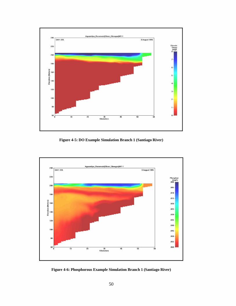
50
Figure 4-5: DO Example Simulation Branch 1 (Santiago River)
Figure 4-6: Phosphorous Example Simulation Branch 1 (Santiago River)

51
Figure 4-7: Chlorophyll α Example Simulation Branch 1 (Santiago River)
Figure 4-8: Cyanobacteria Example Simulation Branch 1 (Santiago River)

52
4.4 Monitoring and Data Acquisition Plan
As a result of developing the CE-QUAL-W2 water quality model for the
Aguamilpa reservoir, a monitoring and data acquisition plan was designed to obtain the
minimum required data necessary to support water quality modeling with CE-QUAL-W2
for the Aguamilpa reservoir. This monitoring and data acquisition plan includes the
following data:
• Hourly climatological data from the station located in the Aguamilpa-
Solidaridad Dam. This station is known as Aguamilpa or Carrizal and the
acquisition of this data from 1994 to 2007 is still in process. These data
can be obtained from CFE (Tepic) and from the website created by CFE:
<http://h06814.iie.org.mx/presascfe/semanapresaCaracol.aspx?estacion=
Agu>. It is important to mention that this website was uploaded on the
last week of July 2008 and it only has climatological data from October
2007 to the present.
• Daily inflow data from the gauging stations known as La Playa,
Huaynamota II (or Jesús María and Chapalagana), Cerro Blanco and the
average daily outflow data from El Cajon Dam which is located upstream
of the Aguamilpa reservoir (see Appendix A). All these data can be
obtained from CFE (Tepic station and Mexico City) and CONAGUA.
The acquisition of these data is still in process.
• Hourly releases and observed surface water level values from the
Aguamilpa-Solidaridad Dam. These data were obtained from CFE
(Tepic) and CFE (Mexico City) for the initial model, and should continue
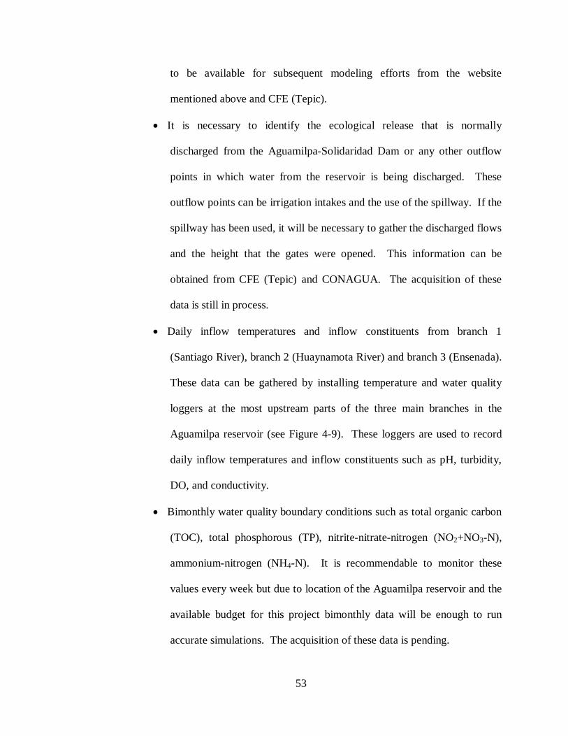
53
to be available for subsequent modeling efforts from the website
mentioned above and CFE (Tepic).
• It is necessary to identify the ecological release that is normally
discharged from the Aguamilpa-Solidaridad Dam or any other outflow
points in which water from the reservoir is being discharged. These
outflow points can be irrigation intakes and the use of the spillway. If the
spillway has been used, it will be necessary to gather the discharged flows
and the height that the gates were opened. This information can be
obtained from CFE (Tepic) and CONAGUA. The acquisition of these
data is still in process.
• Daily inflow temperatures and inflow constituents from branch 1
(Santiago River), branch 2 (Huaynamota River) and branch 3 (Ensenada).
These data can be gathered by installing temperature and water quality
loggers at the most upstream parts of the three main branches in the
Aguamilpa reservoir (see Figure 4-9). These loggers are used to record
daily inflow temperatures and inflow constituents such as pH, turbidity,
DO, and conductivity.
• Bimonthly water quality boundary conditions such as total organic carbon
(TOC), total phosphorous (TP), nitrite-nitrate-nitrogen (NO2+NO3-N),
ammonium-nitrogen (NH4-N). It is recommendable to monitor these
values every week but due to location of the Aguamilpa reservoir and the
available budget for this project bimonthly data will be enough to run
accurate simulations. The acquisition of these data is pending.
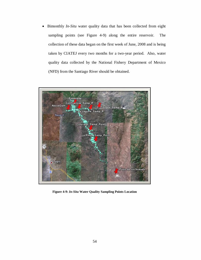
54
• Bimonthly In-Situ water quality data that has been collected from eight
sampling points (see Figure 4-9) along the entire reservoir. The
collection of these data began on the first week of June, 2008 and is being
taken by CIATEJ every two months for a two-year period. Also, water
quality data collected by the National Fishery Department of Mexico
(NFD) from the Santiago River should be obtained.
Figure 4-9: In-Situ Water Quality Sampling Points Location

55
5 Summary and Conclusions
A water quality model was identified and assessed for a subtropical reservoir,
Aguamilpa. The Aguamilpa reservoir, located in the State of Nayarit, Mexico, is
important for the northwest area of the country for power generation, irrigation, and
fishing. Furthermore, the government’s future plans show that it may be used for water
supply. Because most of the Mexican reservoirs present different levels of pollution, the
use of a two-dimensional CE-QUAL-W2 water quality modeling tool might help
authorities, researchers, and private institutions better manage the reservoirs. This study
concluded that the CE-QUAL-W2 water quality model is applicable to large-narrow-deep
subtropical reservoirs, like Aguamilpa, if the minimum required data are available.
Objectives were established for this study and their realization is explained below as well
as future work for this study.
First of all, developing the CE-QUAL-W2 water quality model for the Aguamilpa
reservoir demonstrated that this model is appropriate to simulate the Aguamilpa reservoir
(subtropical). The characteristics of the area where it is located and the capabilities of the
model were useful to conclude the CE-QUAL-W2 suitability. The model was built for
1995 and 1996 due to the availability of data.

56
The minimum required data and gaps for modeling the Aguamilpa reservoir were
identified during and after the construction of the CE-QUAL-W2 water quality model.
As discussed in previous sections, there were unavailable or incomplete data required for
modeling the reservoir and it was necessary to make several assumptions that could affect
the accuracy of the model. In this study, it was found that most of the required data can
be obtained from Mexican governmental agencies such as INEGI, CFE (Tepic and
Mexico City) and CONAGUA. Obtaining data is a time consuming task because the data
are spread throughout the offices previously mentioned. However, this study explained
what kind of data are needed and where it can be gathered or requested.
Even though the unavailable inflow water temperature data, thermal simulations,
illustrated in the results section, were run to model the water temperatures in the reservoir
during different weather seasons over a two-year simulation period. These thermal
simulations showed that the Aguamilpa reservoir is stratified during most part of the year,
turning over once per year during the month of December (monomictic reservoir) which
is a typical behavior for a deep subtropical reservoir. These simulations were compared
with the few water temperature data collected in the field and show these thermal
simulations are close to what was happening in the reservoir. This preliminary thermal
calibration reinforced the fact that CE-QUAL-W2 is suitable for the Aguamilpa reservoir.
This study also concluded that it is important to frequently monitor the inflow water
temperature for the three main modeled branches (Santiago River, Huaynamota River and
Ensenada) to have enough data for thermal calibrations. Running the example water
quality simulations illustrated what water quality data are required for modeling the
reservoir. Like thermal simulations, the example water quality simulations helped design
57
a water quality-quantity monitoring and data acquisition plan used to obtain all the
minimum required data to run an accurate model.
The monitoring and data acquisition plan designed in this study detail when,
where, and what data should be collected. This plan should be implemented as soon as
possible and followed to update and calibrate the model. It may be challenging to follow
this monitoring plan because the current budget for this project may be insufficient to
finance the field trips to the reservoir and purchase the required equipment.
Nevertheless, if this monitoring and data acquisition plan is correctly followed, the model
can be updated and calibrated. Once the model is calibrated, it may be a useful
monitoring tool to simulate the water quality changes in the Aguamilpa reservoir
(subtropical) and be used to evaluate the environmental, climatological and
anthropogenic effects of various management choices. It also serves as a guideline for
developing similar water quality models at other reservoirs in the region.
The developed CE-QUAL-W2 water quality model for the Aguamilpa reservoir
requires continuing work. The results from this study have generated new options for
future research work which include: 1) Optimizing the proposed water quality monitoring
plan, 2) Updating the CE-QUAL-W2 water quality model based on the ongoing water
quality data being collected at Aguamilpa, 3) Continue collecting In-Situ water quality
data, 4) Calibration of the model, 5) Simulating different water quality scenarios to
provide information for management plans, 6) Identifying and adding algal groups to the
model, 7) Providing guidelines for development of models for similar reservoirs located
along the Santiago River and other locations in Mexico.

58

59
References
Aquaveo. (2008). "AQUAVEO Water Modeling Solutions." http://www.aquaveo.com/wms (October/15, 2008).
Arredondo, J. L., Diaz, G., and Ponce, J. T. (2008). Limnologia de Presas Mexicanas:
Aspectos Teoricos y Practicos. Universidad Autonoma Metropolitana and Agt Editor SA.
Avery, R. E. (2007). "Evaluating the impact of nutrient input reductions on chlorophyll a
concentrations using CE-QUAL-W2 at Lake Eucha, Oklahoma." MS thesis, University of Arkansas, Arkansas, United States.
Ayres, W.S., Busia, A., Dinar, A., Hirji, R., Lintner, S.E., McCalla, A.F., and Robelus, R.
(1997). "Integrated Lake and Reservoir Management. World Bank Approach and Experience." Rep. No. 358, The World Bank, Washington, D.C.
Bowen, J. D., and Hieronymus, J. W. (2003). "A CE-QUAL-W2 Model of Neuse Estuary
for Total Maximum Daily Load Development." J.Water Resour.Plann.Manage., 129(4), 283-294.
Chapra, S. C. (1997). Surface Water Quality Modeling. McGraw-Hill, New York, United
States. Cloern, J. E. (2001). "Our evolving conceptual model of the coastal eutrophication
problem." Mar Ecol Prog Ser, 210 223-253. Cole, T.M., and S.A. Wells. (2003). "CE-QUAL-W2: A two-dimensional, laterally
averaged, Hydrodynamic and Water Quality Model, Version 3.2." Rep. No. Instruction Report EL-03-1, US Army Engineering and Research Development Center, Vicksburg, MS.
Cole, T.M., and Tillman, D.H. (2001). "Water Quality Modeling of Allatoona and West
Point Reservoirs Using CE-QUAL-W2." Rep. No. ERDC/EL SR-01-3, Environmental Laboratory U.S. Army Engineer Research and Development Center.
60
Comision Federal de Electricidad [CFE]. (2002). "Informe Final de los Estudios
Hidrologicos e Hidraulicos." Comision Federal de Electricidad, Nayarit, Mexico. Comision Federal de Electricidad [CFE]. (1991). "Proyecto Hidroelectrico Aguamilpa,
Nay. Mexico 1991." Comision Federal de Electricidad. Comision Nacional del Agua [CONAGUA]. (2008). "National Water Program 2007-
2012." Secretaria de Medio Ambiente y Recursos Naturales, D.F., Mexico. de Victorica, J. L. (1996). "Modelo para Simular la Evolucion del Oxigeno Disuelto en
Embalses." Ingenieria Del Agua, 3(2), 63-74. de Victorica, J.L., Galvan, M., and Rojas, M.N. (1993). "Impacto a la Calidad del Agua
por el Proyecto Hidroelectrico Aguamilpa, Nay." Rep. No. 1303, Comision Federal de Electricidad, Mexico.
Friedler, E., Juanico, M., and Shelef, G. (2003). "Simulation model of wastewater
stabilization reservoirs." Ecol.Eng., 20(2), 121. GRUBA, S.A. de C.V. [GRUBA]. (1997). "Estudio de Calidad del Agua en el Embalse
de la Presa Aguamilpa, Nayarit." Rep. No. GSCA 007/97, Comision Nacional del Agua Subdireccion General Tecnica Gerencia de Saneamiento y Calidad del Agua, Nayarit, Mexico.
Hellyer, G. (2008). "Some Landscape and Spatial Analysis Tools and Datasets for Rapid
Watershed Assessment - Short Version." United States Environmental Protection Agency, New England, United States.
Holiday-Weather. (2007). "Holiday-Weather.com. Daily Worldwide forecasts for your
holiday." http://www.holiday-weather.com/aguamilpa_mx/index.html (May/30, 2008).
Horne, A.J., and Goldman, C.R. (1994). Limnology. McGraw-Hill, United States. Huszar, L. M., Caraco, N. F., Roland, F., and Cole, J. (2006). "Nutrient–chlorophyll
relationships in tropical–subtropical lakes: do temperate models fit?" Biogeochemistry, 79(1/2), 239.
Hutchinson, G. E. (1957). A Treatise on Limnology. John Wiley and Sons, New York,
NY.

61
INEGI. (2008). "Instituto Nacional de Estadistica y Geografia. Sistema Nacional de Informacion Estadistica y Geografia. Sistema de Descarga del Continuo de Elevaciones Mexicano." http://mapserver.inegi.org.mx/DescargaMDEWeb/?s=geo&c=977 (January/7, 2008).
INEGI. (2007). Sintesis de Informacion Geografica Estatal SIGE Nayarit. Instituto
Nacional de Estadistica Geografia e Informatica (CD-ROM), Mexico. INP. (2006). "Dictamen para la implementacion de la veda 2006, Aguamilpa, Nayarit.
Instituto Nacional de la Pesca. Centro Regional de Investigacion Pesquera Bahia de Banderas, Nayarit. Secretaria de Agricultura, Ganaderia, Desarrollo Rural, Pesca y Alimentacion." http://www.inp.sagarpa.gob.mx/Dictamenes/2006/dictamenvedatilapiaaguamilpa2006.pdf. (January/7, 2008).
IUCN., and. WB. (1997). "Large Dams. Learning from the Past Looking at the Future.
Workshop Proceedings. Gland, Switzerland." The World Conservation Union and the World Bank, Gland, Switzerland.
Kuo, J., Lung, W., Yang, C., Liu, W., Yang, M., and Tang, T. (2006). "Eutrophication
modelling of reservoirs in Taiwan." Environmental Modelling & Software, 21(6), 829-844.
Lewis, W. M. J. (2002). "Causes for the high frequency of nitrogen limitation in tropical
lakes." Verh. Internat. Verein. Limnol, 28 210-213. Loginetics. (2008). "Reservoir Modeling Tools."
http://www.loginetics.com/modtools/2DMOD.html (August/30, 2008). MacKinnon, M.R., and Herbert, B.W. (1996). "Temperature, Dissolved Oxygen and
Stratification in a Tropical Reservoir, Lake Tinaroo, Northern Queensland, Australia." Mar. Freshwater Res, 47(7), 937-949.
Marengo, H. (2006). "Case Study: Dam Safety during Construction, Lessons of the
Overtopping Diversion Works at Aguamilpa Dam." J.Hydraul.Eng., 132(11), 1121-1127.
Martin, J.L., and McCutcheon, S.C. (1999). Hydrodynamics and Transport for Water
Quality Modeling. Lewis Publishers, Boca Raton, Fla. Mazumder, A., and Havens, K.E. (1998). "Nutrient-chlorophyll-Secchi relationships
under contrasting grazer communities of temperate versus subtropical lakes." Can. J. Fish. Aquat. Sci, 55 1652-1662.
62
McLachlan, A. J. (1974). "Development of Some Lake Ecosystems in Tropical Africa, with Special Reference to the Invertebrates." Biol. Rev, 49(3), 365-397.
Nelson, E. J. (2006). WMS 8.0 HTML Help Document. Environmental Modeling
Research Laboratory, Brigham Young University, Provo, UT. Nielsen, E. J. (2005). "Algal Suscession and Nutrient Dynamics in Elephant Butte
Reservoir." MS thesis, Brigham Young University, Provo, UT. NOAA. (2008). "NOAA Satellite and Information Service."
http://www.ncdc.noaa.gov.erl.lib.byu.edu/oa/ncdc.html (April/25, 2008). OEPA. (2008). "TMDLs for the Black River Watershed, Ohio. Appendix D: CE-QUAL-
W2 Modeling Report." Ohio Environmental Protection Agency, Ohio, US. Ortiz, M.A., de Anda, J., and Maniak, U. (2006). "Estimation of Trophic States in Warm
Tropical Lakes and Reservoirs of Latin America by Using GPSS Simulation." Interciencia, 31(5), 345-350.
Portland State University [PSU]. (2008). "Water Quality Research Group. CE-QUAL-
W2 Hydrodynamic and Water Quality Model." http://www.ce.pdx.edu/w2/ (August/2, 2008).
Potential Impacts. (2003). "Potential Impacts of the Rio Lerma-Lago Chapala-Rio
Santiago Watershed on the Presa de Aguamilpa Fishery. Interim Report." PSOMAS. (2002). "Deer Creek Reservoir Drainage TMDL Study." Prepared for Utah
Department of Environmental Quality Division of Water Quality. Prepared by PSOMAS, Salt Lake City, UT.
Raftis, R. R. (2007). "Internal Cycling in an Urban Drinking Water Reservoir." MS
thesis, Indiana University-Purdue University, Indianapolis, IN. Reddy, M. V. (2005). Restoration and Management of Tropical Eutrophic Lakes. Science
Publishers, Inc, Enfield, NH. ROP. (1997). "Ficha Tecnica: Central Hidroelectrica de Aguamilpa." Revista de Obras
Publicas, 3(363), 116-117. Shrestha, R. (2006). "Water Temperature Simulation in Amistad Reservoir." MS thesis,
Lamar University, Beaumont, Texas. U.S. Environmental Protection Agency [EPA]. (2007). "Water Quality Models and
Tools." (July/27, 2008).
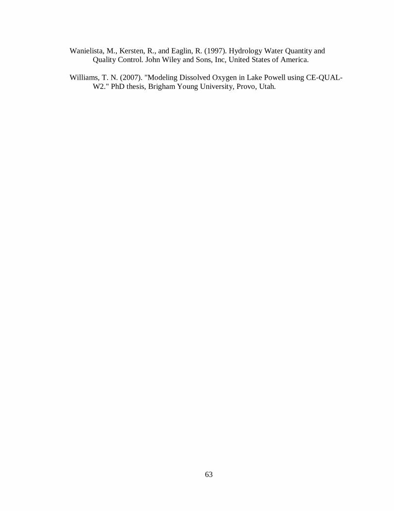
63
Wanielista, M., Kersten, R., and Eaglin, R. (1997). Hydrology Water Quantity and Quality Control. John Wiley and Sons, Inc, United States of America.
Williams, T. N. (2007). "Modeling Dissolved Oxygen in Lake Powell using CE-QUAL-
W2." PhD thesis, Brigham Young University, Provo, Utah.

64
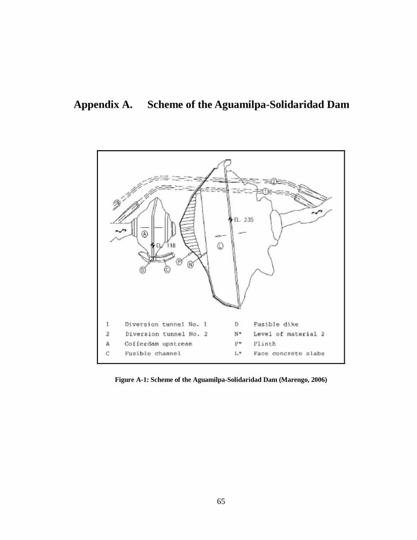
65
Appendix A. Scheme of the Aguamilpa-Solidaridad Dam
Figure A-1: Scheme of the Aguamilpa-Solidaridad Dam (Marengo, 2006)

66
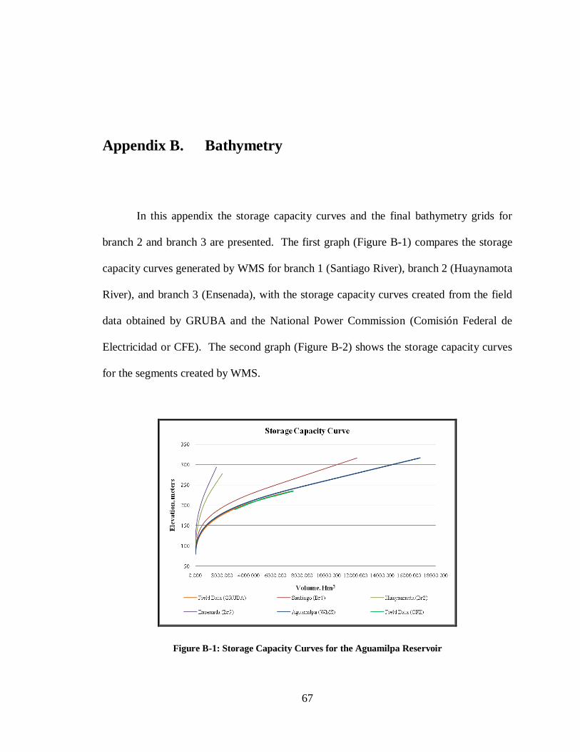
67
Appendix B. Bathymetry
In this appendix the storage capacity curves and the final bathymetry grids for
branch 2 and branch 3 are presented. The first graph (Figure B-1) compares the storage
capacity curves generated by WMS for branch 1 (Santiago River), branch 2 (Huaynamota
River), and branch 3 (Ensenada), with the storage capacity curves created from the field
data obtained by GRUBA and the National Power Commission (Comisión Federal de
Electricidad or CFE). The second graph (Figure B-2) shows the storage capacity curves
for the segments created by WMS.
Figure B-1: Storage Capacity Curves for the Aguamilpa Reservoir

68
Figure B-2: Segments Storage Capacity Curves Generated by WMS
The final bathymetry grids of the Aguamilpa reservoir model are shown in Figure
B-3 and Figure B-4.

69
Figure B-3: W2 Bathymetry Grid of Branch 2 (Huaynamota River)
Figure B-4: W2 Bathymetry Grid of Branch 3 (Ensenada)

70

71
Appendix C. Control File

72

73
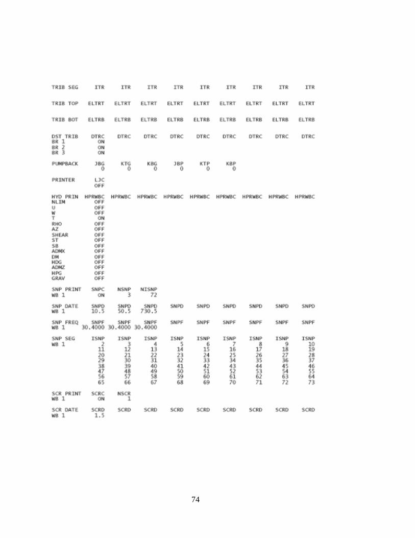
74

75

76

77

78

79

80

81
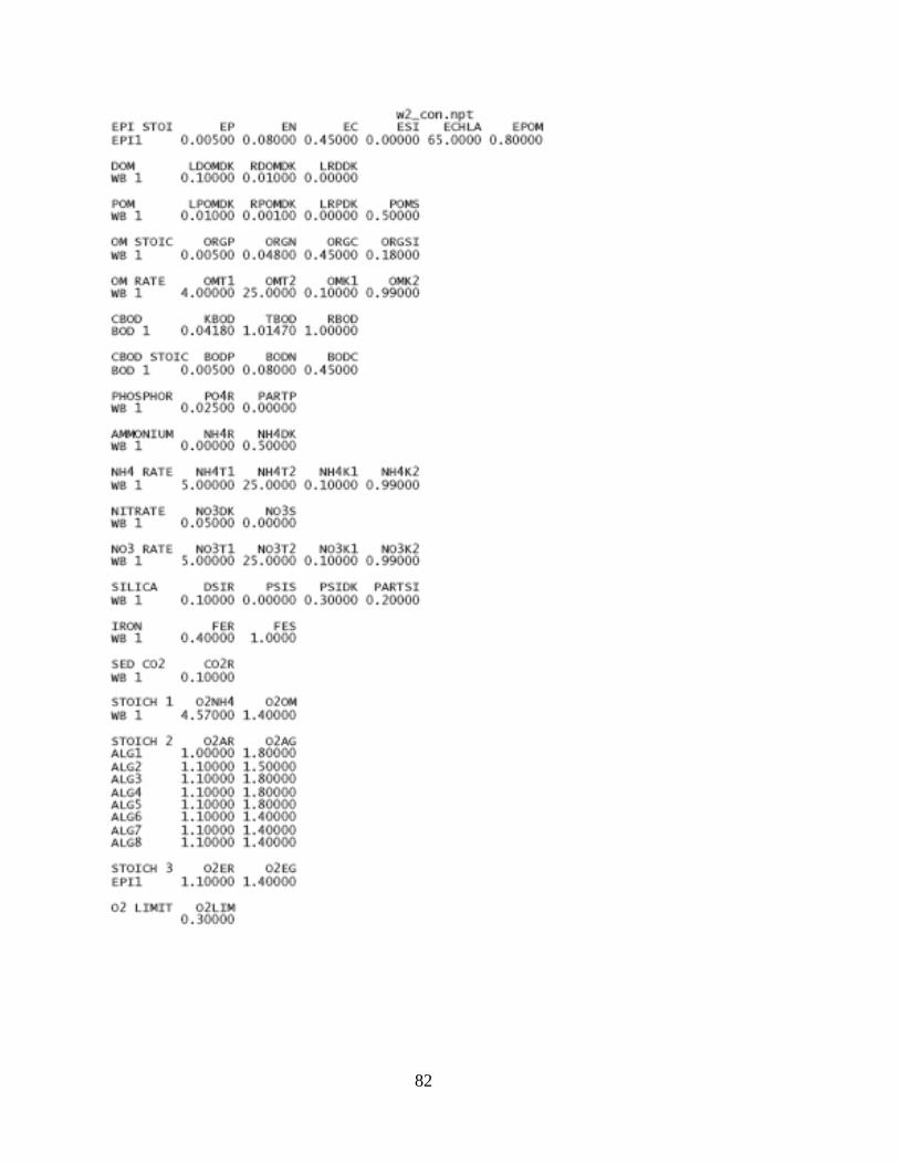
82
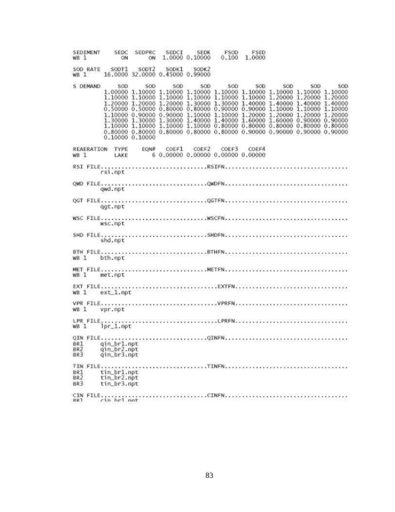
83
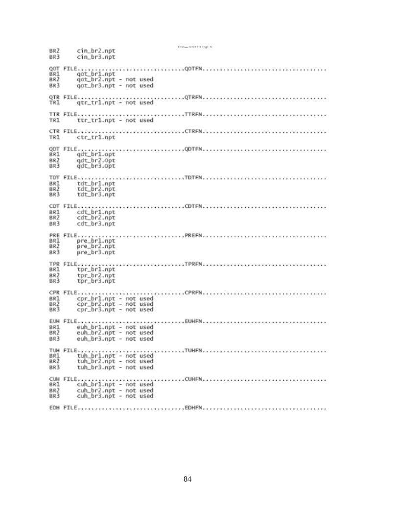
84
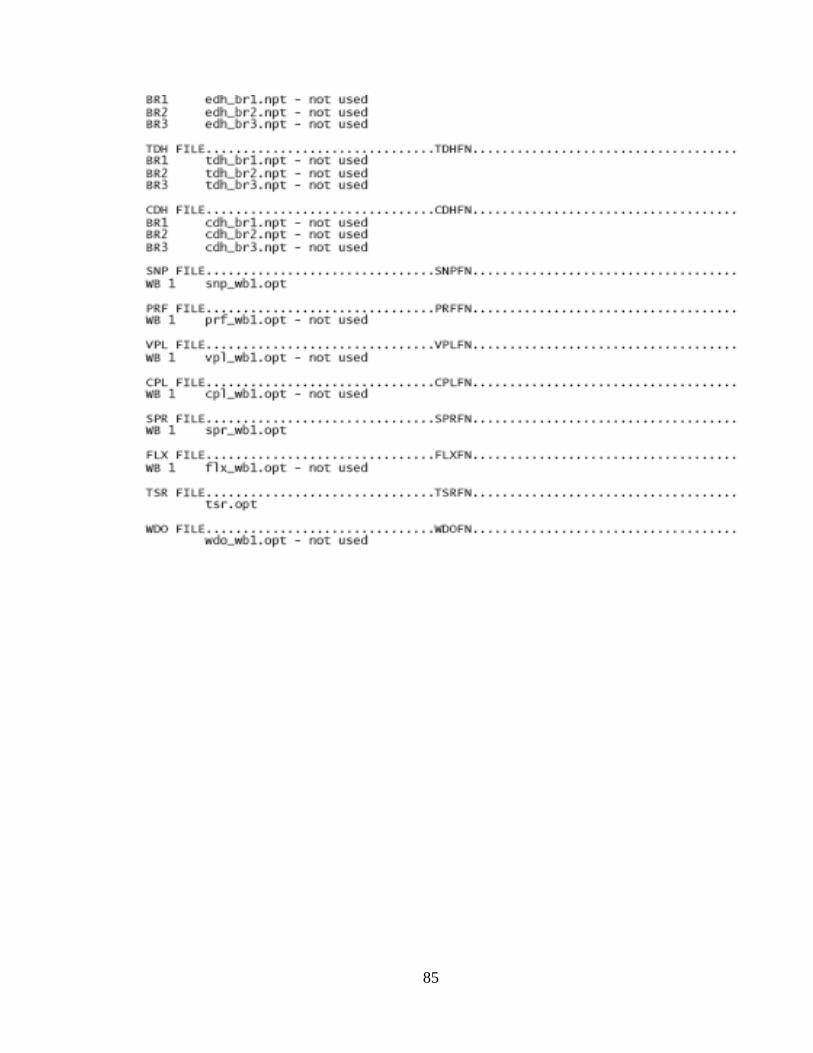
85

86

87
Appendix D. CFE Dams and Gauging Stations Location
Figure D-1: Hydrographic Scheme of the Santiago River

88