assessing agricultural consumptive useucrcommission.com/repdoc/studies/assessing...
TRANSCRIPT
Assessing Agricultural
Consumptive Usein the Upper Colorado River Basin
P h a s e 1november 2013
Hydrologic Engineering, Inc.
TABLE OF CONTENTS
N:\PROJECTS\22243147_UPPER_CO_LOSSES\12.0_WORD_PROC\FINAL_REPORT\ASSESSING AGRICULTURAL CONSUMPTIVE USEFINAL.DOCX\31-DEC-13\\ i
Executive Summary ............................................................................................................................... ES-1
Section 1 ONE Introduction ..................................................................................................................... 1-1
Introduction .............................................................................................. 1-1 1.1
Section 2 TWO Current Methodologies and Status ............................................................................... 2-1
Definitions................................................................................................ 2-1 2.1 Irrigated Acreage Assessment Availability and Attribution .................... 2-4 2.2 Climate Station Data Availability ............................................................ 2-5 2.3 Potential Crop Consumptive Use Calculation Methods .......................... 2-8 2.4 Effective Precipitation Estimation Methods .......................................... 2-10 2.5 Water Supply Data Availability ............................................................. 2-10 2.6 Water Supply-Limited Consumptive Use Calculation Methods ........... 2-13 2.7 Crop Consumptive Use Models ............................................................. 2-13 2.8
Section 3 THREE Potential Applicable Methodologies ............................................................................. 3-1
Potential Application of Remote Sensing Methods ................................. 3-1 3.13.1.1 Background and Objectives ......................................................... 3-1 3.1.2 Review of Traditional and Ground-Based Consumptive Use
Estimating Methods ..................................................................... 3-2 3.1.3 Factors Affecting Actual Crop Evapotranspiration ..................... 3-3 3.1.4 Resolution Issues Related to Irrigated Agriculture ...................... 3-4
Radiation and Energy Balance Terminology and Concepts .................... 3-4 3.23.2.1 Components of the Radiation Balance ......................................... 3-4 3.2.2 Components of the Energy Balance ............................................. 3-6 3.2.3 Satellite Platforms Suitable for Radiation and Energy
Balance Applications in Irrigated Agriculture ............................. 3-7 Example Thermal Band Application to Radiation and Energy 3.3
Balance ..................................................................................................... 3-8 3.3.1 Description of Field Experiment .................................................. 3-9 3.3.2 Remote Sensing Data Processing ................................................. 3-9 3.3.3 Results: Instantaneous Energy Balance at a Point .................... 3-10 3.3.4 Interpolation between Scenes of Satellite Overpass .................. 3-11 3.3.5 Results: Spatial Distribution of Actual Evapotranspiration ...... 3-13 3.3.6 Sample Results from Other Investigations ................................ 3-13 3.3.7 Comparison of Meteorological-Based Methods With
Remote Sensing-Based Methods ............................................... 3-15 Alternative Data Processing Procedures ................................................ 3-15 3.4
3.4.1 RESET ....................................................................................... 3-15 3.4.2 ArcGIS Using Python and Other Procedures............................. 3-15 3.4.3 TOPS-SIMS ............................................................................... 3-16 3.4.4 Automated METRIC Procedure ................................................ 3-16
Operational Challenges and Potential Solutions .................................... 3-16 3.5
TABLE OF CONTENTS
N:\PROJECTS\22243147_UPPER_CO_LOSSES\12.0_WORD_PROC\FINAL_REPORT\ASSESSING AGRICULTURAL CONSUMPTIVE USEFINAL.DOCX\31-DEC-13\\ ii
3.5.1 Number and Frequency of Growing Season Clear-Sky Satellite Overpasses ................................................................... 3-16
3.5.2 Masking Cloud Affected Portions of Scenes ............................ 3-17 3.5.3 Accounting for Sloping Ground in Radiation Calculations ....... 3-17 3.5.4 Effects of Higher Elevation on Actual Evapotranspiration ....... 3-17 3.5.5 Availability of Ground-Based Meteorological Data .................. 3-17 3.5.6 Crop-Cutting Between Dates of Satellite Overpasses ............... 3-18 3.5.7 Precipitation (or Irrigation) just before or just after Satellite
Overpass ..................................................................................... 3-18 3.5.8 Application of Cold Irrigation Water to Crops .......................... 3-19 3.5.9 Data Input and Processing Requirements .................................. 3-20
Out of the Box – a Different Approach ................................................. 3-20 3.63.6.1 Uncertainty in Analysis of Landsat Scenes ............................... 3-20 3.6.2 ALEXI and Disalexi Approach .................................................. 3-22 3.6.3 Gap Filling Using Data Fusion .................................................. 3-25
Remote Sensing Recommendations ....................................................... 3-28 3.73.7.1 Definition of Remote Sensing Platform and Data Analysis
Requirements ............................................................................. 3-28 3.7.2 Application of Satellite Remote Sensing Data........................... 3-29 3.7.3 Ground-Based Meteorological and Evaporative Flux
Networks .................................................................................... 3-29 Additional Equations ............................................................................. 3-30 3.8
3.8.1 Sharpening Pixel Level Ts Using High Resolution Optical Band Data for NDVI .................................................................. 3-30
3.8.2 Data Processing for Soil Heat Flux ............................................ 3-31 3.8.3 Iterative Method of Data Processing for Sensible Heat Flux .... 3-32 3.8.4 Cost Estimates of Eddy Covariance and
Micrometeorological Stations .................................................... 3-35
Section 4 FOUR References ...................................................................................................................... 4-1
References ................................................................................................ 4-1 4.1Li
List of Tables
Table 2.1 Irrigated Acreage Assessments
Table 2.2 Climate Station Information
Table 2.3 Potential Consumptive Use Calculation Methods Currently Used
Table 2.4 Water Supply Data
Table 2.5 Consumptive Use Methods and Models
Table 3.1 Extended and basic meteorological stations in Upper Colorado River Basin.
Table 3.2 Current maximum crop ET estimating methods in Upper Colorado River Basin.
TABLE OF CONTENTS
N:\PROJECTS\22243147_UPPER_CO_LOSSES\12.0_WORD_PROC\FINAL_REPORT\ASSESSING AGRICULTURAL CONSUMPTIVE USEFINAL.DOCX\31-DEC-13\\ iii
Table 3.3 Results of analysis of evapotranspiration estimating methods compared to lysimeter data (Jensen, Burman and Allen, 1990).
Table 3.4 Thermal band spatial and temporal resolutions for application to water balance studies.
Table 3.5 Landsat 4, 5, 7 and LDCM (Landsat 8) satellite sensors, band number, band description, bandwidths and ground sample distance (GSD).
Table 3.6 Results of data analysis at a point, i.e. at the Bowen ratio stations and combination of nine Landsat scenes centered at the Bowen ratio station, integrated over the irrigation season (01 May to 30 Sep) and integrated over the irrigated and unirrigated land areas within the Wood River Valley.
Table 3.7 Lysimeter measured ET versus instantaneous estimated ET using METRIC at time of satellite overpass, Kimberly, ID.
Table 3.8 Example of comparison of meteorological-based methods with remote sensing-based methods
Table 3.9 Sources of nput data for the ALEXI and DisALEXI models (Anderson et al., 2004).
Table 3.10 Comparison of Major Attributes of Thermal Band Remote Sensing Platforms.
Table 3.11 Comparison of Major Attributes of Thermal Band Remote Sensing Methods for Actual ET Using METRIC and ALEX I/DisALEXI Computational Algorithms.
Table 3.12 Equipment Cost Estimate for combined eddy covariance-energy balance and micrometeorological station.
Table 3.13 Equipment Cost Estimate for Eddy Covariance Network Support.
Table 3.14 Equipment Cost estimate for Reference Evapotranspiration Monitoring Station
List of Figures Figure 2.1 General Procedure for Estimating Consumptive Use
Figure 2.2 Climate Station Locations
Figure 2.3 Stream Gage Locations
Figure 3.1 Comparison of images of agricultural fields near Corcoran, Kings County, San Joaquin Valley of California from Google Earth (left) compared to MODIS Satellite ET data retrieval (right, image from SEBAL North America). Note red boxes are indicators of road numbers on both images. (Scenes not taken on same date.)
Figure 3.2 Detail of individual fields from Paraná River Delta (Argentina, Brazil, Paraguay) using Landsat data. Figure on left shows part of the Paraná River Delta with irrigated fields shown in red box and figure at right shows individual fields zooming in on red box.
TABLE OF CONTENTS
N:\PROJECTS\22243147_UPPER_CO_LOSSES\12.0_WORD_PROC\FINAL_REPORT\ASSESSING AGRICULTURAL CONSUMPTIVE USEFINAL.DOCX\31-DEC-13\\ iv
Figure 3.3 (a)Landsat scene of NDVI (grey-scale from 0 to 288) for Wood River Valley, Oregon. (b) Pixelated view of same scene indicating 30-m resolution of red and near infrared reflectance near center of the scene.
Figure 3.4 Whisk-broom data acquisition system of Landsat 1 through 7 compared to push-broom data acquisition system on LDCM (Landsat 8). (Image courtesy of NASA LDCM brochure.)
Figure 3.5 Comparison of Landsat 7 and LDCM (Landsat 8) bands and wavelengths. Note that the band 9 on Landsat 8 (1.360 to 1.390 μm) will have enhanced cloud detection capabilities. (Image courtesy of NASA LDCM brochure.)
Figure 3.6 Bowen ratio station at KL03 (unirrigated site), Thomas Ranch, April 2004. Notice excellent fetch conditions which are on the order of 1,000 m of uniform ground cover in the predominant upwind direction. (From Cuenca et al., 2013, permission requested.)
Figure 3.7(a) Energy balance for net radiation (Rnet), soil heat flux (G), sensible heat flux (H), and latent heat flux (or evapotranspiration) (LE) every 20-min measured by the Bowen ratio system at KL03 (unirrigated) site for DOY 288 (14 October) 2004. (From Cuenca et al., 2013, permission requested.)
Figure 3.7(b) Energy balance for net radiation (Rnet), soil heat flux (G), sensible heat flux (H), and latent heat flux (or evapotranspiration) (LE) every 20-min measured by the Bowen ratio system at KL04 (irrigated) site for DOY 288 (14 October) 2004. (From Cuenca et al., 2013, permission requested.)
Figure 3.8 Results of the Landsat data analysis for components of the energy balance from four Landsat scenes for the unirrigated site (KL03) in the Wood River Valley, Oregon, 2004 compared to Bowen ratio station measurements. (From Cuenca et al., 2013, permission requested.)
Figure 3.9 Results of the Landsat data analysis for components of the energy balance from four Landsat scenes for the irrigated site (KL04) in the Wood River Valley, Oregon, 2004 compared to Bowen ratio station measurements. (Note: Not all ground-based sensors were operational at this site during the time of satellite overpass in April.) (From Cuenca et al., 2013, permission requested.)
Figure 3.10 Theoretical value of the evaporative fraction as function of available energy, Rn – G, for moderate climatic conditions and for freely transpiring vegetation (rs = 50 s/m) as well as vegetation exhibiting moderate stomatal resistance (rs – 100 s/m).
Figure 3.11 Plot of midday evaporative fraction (i.e. Rn > 300 W/m2) over pasture in the Wood River Valley, Oregon, for unirrigated site, KL03, and irrigated site, KL04, for 11 days late in growing season in 2004.
Figure 3.12(a) Results of the Landsat data analysis for spatially distributed actual ET in the Wood River Valley, Oregon for Landsat 7 scenes from 22 April and 25 June, 2004. (From Cuenca et al., 2013, permission requested.)
Figure 3.12(b) Results of the Landsat data analysis for spatially distributed actual ET in the Wood River Valley, Oregon for Landsat 7 scenes from 27 July and 28 August, 2004. (From Cuenca et al., 2013, permission requested.)
TABLE OF CONTENTS
N:\PROJECTS\22243147_UPPER_CO_LOSSES\12.0_WORD_PROC\FINAL_REPORT\ASSESSING AGRICULTURAL CONSUMPTIVE USEFINAL.DOCX\31-DEC-13\\ v
Figure 3.13 ALEXI/DisALEXI approach. 5-km scale latent heat fluxes using GOES satellite input data over Oklahoma are disaggregated to 30-m scale using sharpened Landsat thermal band data. (From Anderson et al., 2004, permission requested.)
Figure 3.14 Schematic diagram of ALEXI/DisALEXI modeling scheme showing surface temperature and vegetation cover fraction as function of directional view angle, φ. The two-source model is coupled with an atmospheric boundary layer simulation model to estimate the air temperature at 50-m above the ground and this temperature is then used to downscale atmospheric processes to 30-m using Landsat thermal band data. (From Kustas et al., 2013, permission requested.)
Figure 3.15 Example application of four “blending” algorithms for Landsat and MODIS data to maintain the spatial resolution of Landsat data and the temporal resolution of MODIS data over the Lower Gwydir Catchment study site in New South Wales, Australia. Observed Landsat data are in left-most column, estimated results for the algorithms in the four right-most columns with the algorithm labeled at the top. (From Emelyanova et al., 2012, permission requested.)
Figure 3.16 Example application of ALEXI-DisALEXI downscaling together with the STARFM interpolating algorithm for daily evapotranspiration over nine days near Orlando, FL in 2002. This study required application of GOES, MODIS and Landsat data. (From Anderson et al., 2013, with permission).
Figure 3.17 Left: Close up of reference ET fraction, ETrF, image from an area near Christmas Valley, Oregon on 17 June 2004. Right: The same ETrF map but calculated using “sharpened” surface temperature based on NDVI distribution. (From Allen, 2012, with permission.)
List of Appendices Appendix A Colorado Appendix B New Mexico Appendix C Utah Appendix D Wyoming Appendix E Reclamation Appendix F Upper Colorado River Basin Compact, 1948
EXECUTIVE SUMMARY
N:\PROJECTS\22243147_UPPER_CO_LOSSES\12.0_WORD_PROC\FINAL_REPORT\ASSESSING AGRICULTURAL CONSUMPTIVE USEFINAL.DOCX\31-DEC-13\\ ES-1
The four states of the Upper Division(Colorado, New Mexico, Utah and Wyoming), through the Upper Colorado River Commission, requested that the United States Bureau of Reclamation (Reclamation) initiate a study on assessing and improving consumptive use determinations. Reclamation then contracted with a consultant team led by URS, with assistance from CH2M HILL, Wilson Water Group, and Hydrologic Engineering Inc. to review and document the consumptive use methodologies used by the four Upper Division States and Reclamation, and to report on the state of the art of remote sensing for consumptive use calculations and its potential applicability to the Upper Colorado River Basin (Upper Basin). The assessment is limited to the beneficial consumptive uses associated direct irrigation; and does not address other consumptive use and loss components in the Upper Basin. The study team wishes to thank the technical staff of the four Upper Division States, the Upper Colorado River Commission (UCRC) staff, and Reclamation staff – in particular staff at the Technical Services Center in Denver – for their technical assistance on the project. The intent of the study was to: 1) Identify the differences in consumptive use methodologies used by the four states and
Reclamation, 2) Provide the basis for a discussion among these entities as to whether changes to the methodology
used by Reclamation are appropriate at this time, and 3) Provide a recommendation as to whether the current state of the art of remote sensing is
sufficiently advanced for the Upper Division States and Reclamation to further investigate its implementation within the Upper Basin.
Water allocation among the Colorado River Basin states is stipulated by the Colorado River Compact of 1922, the Mexican Treaty of 1944, and the Upper Colorado River Compact of 1948. These are the principal (but not the sole) documents of the “Law of the River.” This report focuses on estimation of consumptive use by irrigated agriculture in the four states that make up the Upper Division States. Article VI of the Upper Colorado River Compact directs that the UCRC shall determine the quantity of consumptive use of water; Article VIII directs that the UCRC shall have the power to, among other things, make findings as to the quantity of water used each year in the Upper Basin and in each state, make findings as to the quantity of water deliveries at Lee Ferry during each water year, and make findings as to the necessity for and the extent of curtailment of use. Additionally the UCRC is directed to make and transmit an annual report covering its activities to the governors of the Upper Division states and the president. Reclamation is directed by Title VI of the 1968 Colorado River Basin Project Act (PL 90-537) to make reports of the annual consumptive uses and losses, on a five-year basis, beginning with the period starting on October 1, 1970. They are further directed to prepare these reports in consultation with the states and the UCRC, and to report to the president, the Congress, and to the governors of the states signatory to the Colorado River Compact. They are to also condition any contracts for delivery of water originating from the Colorado River Basin upon the availability of water under the Colorado River Compact. Since 1971, Reclamation has both estimated and reported Upper Basin consumptive use in the Consumptive Uses and Losses Report.
EXECUTIVE SUMMARY
N:\PROJECTS\22243147_UPPER_CO_LOSSES\12.0_WORD_PROC\FINAL_REPORT\ASSESSING AGRICULTURAL CONSUMPTIVE USEFINAL.DOCX\31-DEC-13\\ ES-2
Efficient administration of the Colorado River Compact requires accurate estimates of agricultural consumptive use within the basin; as more than 80 percent of the total consumptive use of water within the basin is by irrigated agriculture. As the demands on the water resources of the Colorado River intensify, it will become more important to document both the potential consumptive use, (PCU) (the amount of water the crop would use if given a full supply) as well as the actual consumptive use, (actual CU) (the amount the crop actually consumed). Many areas in the Upper Basin consistently exist on a “short supply,” depending upon direct flow or limited reservoir storage to supply their crops. The accurate and defensible calculation and reporting of the shortages that the Upper Basin incurs during its normal operations will be necessary in any future negotiations on shortage allocations. CURRENT METHODOLOGIES Section 2 of this report documents the methods, models, and available information that the Upper Division States and Reclamation currently use to estimate PCU and actual CU for irrigated lands in the Upper Colorado River Basin, and other areas of each state. Section 2 provides information that supports the overall project goal of developing a coordinated long-term process among the Upper Division States to estimate consumptive use for irrigated lands in the entire Upper Basin. Details for each state and Reclamation are provided as appendices, and are summarized in Section 2. The availability of the following types of information was assessed during this effort:
• Irrigated Acreage Assessments, including frequency of updates, attribution (e.g., crop type, source, irrigation method) of the irrigated land, and ease of obtaining the information.
• Climate Station Data, including the number and locations of climate stations and the types of climate data parameters collected at each station.
• Water Supply Data, including streamflow gage data and recorded diversion data. The availability of these types of information throughout the Upper Basin influences the PCU and actual CU methods and models that are used by the states and Reclamation. The investigation yielded the following important insights and recommendations with respect to measured data:
• States and Reclamation perform detailed irrigated acreage assessments on an approximately five-year frequency, with the exception that New Mexico performs annual assessments.
• The level of detail varies in terms of attribution and field verification. • Temperature and precipitation climate station data are considered good throughout the
Upper Basin in terms of location and historical availability. • Climate stations that record additional parameters, including wind speed, solar radiation,
and relative humidity are not located with adequate spatial coverage throughout the Upper Basin to represent climate in areas of irrigated acreage.
EXECUTIVE SUMMARY
N:\PROJECTS\22243147_UPPER_CO_LOSSES\12.0_WORD_PROC\FINAL_REPORT\ASSESSING AGRICULTURAL CONSUMPTIVE USEFINAL.DOCX\31-DEC-13\\ ES-3
• Measured river diversions to irrigation are not available in many areas of the Upper Basin.
• Streamflow gage data that can be used as an indication of water supply available to irrigated land provide fair to good coverage on main stem and major tributaries throughout the Upper Basin.
The method most commonly used by each state and Reclamation to estimate PCU is the modified Blaney-Criddle method. This monthly method only requires mean temperature, latitude, and crop type to estimate PCU of irrigated acreage. The detailed Penman-Monteith daily method requiring minimum and maximum temperature, wind speed, solar radiation, and relative humidity, is used in the Green River Basin in Wyoming and in basins other than the Colorado River Basin in each of the Upper Division States. The Penman-Monteith daily method has been accepted by the engineering industry as the most accurate and appropriate method for estimating PCU, per the American Society of Civil Engineers Manual 70 – Evapotranspiration and Irrigation Water Requirements. In addition, the Penman-Monteith method is the most common method used to calibrate remote sensing methods, discussed in Section 3 of this report. To determine the amount of irrigation supply required to meet the PCU, the amount of precipitation that meets a portion of the PCU is estimated. Each state and Reclamation currently use the monthly effective precipitation method outlined in the Soil Conservation Service (SCS) Technical Release 21(TR-21). PCU less effective precipitation is the amount of water that is required from irrigation to provide a full crop irrigation requirement (CIR). Many areas in the Upper Basin do not receive a full irrigation supply each year. The determination of supply-limited consumptive use, or actual consumptive use, requires measurements or estimates of water available to meet CIR. Depending on the extent of measured diversion records, the states and Reclamation take different approaches to estimate actual CU.
• The State of Colorado Division of Water Resources requires that river diversions are measured; therefore, Colorado performs an analysis that compares supply at the ditch level to CIR to estimate actual CU.
• Wyoming measures river diversions on tributaries that require active regulation; the state takes the same approach as Colorado to estimate actual CU in those areas. Where river diversions are not measured, Wyoming estimates actual CU based on shortages for irrigated acreage where diversions are recorded.
• Utah uses a tributary inflow-outflow method to determine water available to irrigated lands; estimated water supply available based on this water balance approach is compared to CIR to estimate actual CU.
• New Mexico routinely measures most river diversions in the San Juan Basin. Records over time indicate that lands irrigated from the San Juan River and the Animas River receive a full supply; therefore, actual CU is estimated to be CIR. Shortages are more common on the La Plate River. Historical diversion records have been used to develop a relationship between measured streamflow and irrigation shortages.
• Reclamation does not use diversion records to determine actual CU; instead they apply a consistent method in the Upper Basin that can be used in areas without measured diversions. Reclamation has tied irrigated areas in the basin to “indicator” streamflow
EXECUTIVE SUMMARY
N:\PROJECTS\22243147_UPPER_CO_LOSSES\12.0_WORD_PROC\FINAL_REPORT\ASSESSING AGRICULTURAL CONSUMPTIVE USEFINAL.DOCX\31-DEC-13\\ ES-4
gages. The amount of flow at those gages is used to estimate shortages and associated actual CU within the respective area.
REMOTE SENSING ASSESSMENT Section 3 of this report evaluates the practicality of applying remote sensing data to calculate actual CU of irrigated areas in the Upper Basin. Investigation of remote sensing techniques included the following:
• Summarizing radiation and energy balance equations and the data required for computation
• Reviewing various methods and their associated accuracies • Discussing common methods used, on a smaller scale, within the Upper Basin • Reviewing results of field studies to determine and document the accuracy of remote
sensing data to the radiation and energy balance equations • Discussing alternative methods for processing the data required for remote sensing
techniques • Identifying operational challenges and potential solutions
In general, a physics-based radiation and energy balance approach utilizing remote sensing data involves converting instantaneous evaporative fluxes at the time of satellite overpass to daily and then seasonal fluxes to estimate the actual CU of irrigated lands during the growing season. Fluxes must be computed at scales relevant to irrigated agricultural fields, ideally on a pixel by pixel basis because an irrigated field adjacent to aunirrigated field will have a very different energy balance. Mean differences in the predicted versus the measured instantaneous evaporative flux at the time of satellite overpass from case studies are on the order of 10 to 15 percent for irrigated fields and 15 to 20 percent for non-irrigated fields. Lower differences for irrigated fields have been noted in some studies and emerging methods appear to be further reducing uncertainty of data analysis. An important outcome of the investigation was to discuss previous concerns with the application of remote sensing methods and how those concerns have been overcome as the methods have been more fully developed. Additional important insights regarding the practicality of applying remote sensing methods include:
• The resolution of thermal band sensors on the LandSat 7 and 8 satellites is sufficient to measure the parameters used in the radiation and energy balance equations for irrigated parcels; and the satellites provide measurements with a combined 8-day temporal resolution.
• It is the current objective of the United States Geological Survey (USGS) LandSat team to make Landsat 7 and 8 data freely available in a timely manner.
• While the assumptions made and the inherent complexity of remote sensing methods yield some uncertainty in accuracy (discussed in this report), application of remote sensing methods is likely more accurate than methods currently used in the Upper Basin.
EXECUTIVE SUMMARY
N:\PROJECTS\22243147_UPPER_CO_LOSSES\12.0_WORD_PROC\FINAL_REPORT\ASSESSING AGRICULTURAL CONSUMPTIVE USEFINAL.DOCX\31-DEC-13\\ ES-5
• Many of the following operational challenges have potential solutions that alleviate or lessen the impact of these challenges during the application of remote sensing methodology.
o Higher elevation crop growth o Areas with significant variations in elevation over satellite scenes o Application of cold water to crops o Separation of irrigated crops from other vegetation o Availability of ground-based climate data for calibration o Required number of images for each irrigation season o Interpolation of data between available scenes o Satellite images with cloud cover o Crop cutting between satellite images
RECOMMENDATIONS: Based on the review and understanding of data availability and methods used to estimate PCU and actual CU by the Upper Basin states and Reclamation, and the investigation into the practicality of implementing remote sensing data gathering and process techniques this report sets forth the following recommendations:
• Develop detailed documentation of the procedures each state uses to develop their irrigated acreage assessment. This will provide a clear understanding of the quality of irrigated acreage data as the basis for Upper Basin PCU estimates.
• Install and maintain an additional 29 climate stations that measure the daily parameters required for the Penman-Monteith PCU method throughout the Upper Basin to ensure adequate spatial coverage.
• Develop protocols for daily climate data quality control, data dissemination, and archiving based on the experience gained from current climate station networks to apply to both existing and recommended additional data collection efforts.
• Continue to investigate the procedures required to move to the Penman-Monteith methodology to estimate PCU throughout the Upper Basin.
• Investigate the applicability of using a monthly as compared to daily effective precipitation analysis with a daily PCU method.
• Investigate alternate methods for estimated actual CU where diversion records do not exist, specifically remote sensing data methods as discussed in Section 3.
• The states and Reclamation should take action to institute a cooperative management approach for consumptive use determinations in the upper basin that would improve coordination and defensibility; increase integrity and independence; address timing and frequency standards; address common standards and quality control and; reduce duplication of effort.
• In the interim, until a comprehensive upper basin consumptive use management structure is instituted, Reclamation should continue to prepare consumptive use and loss reports in coordination with the states and the Commission and the states should continue their current efforts in estimating consumptive uses.
• Develop a protocol to ensure that the method used to determine PCU, actual CU, and agricultural water shortages is consistent for the entire Upper Basin; includes clear

EXECUTIVE SUMMARY
N:\PROJECTS\22243147_UPPER_CO_LOSSES\12.0_WORD_PROC\FINAL_REPORT\ASSESSING AGRICULTURAL CONSUMPTIVE USEFINAL.DOCX\31-DEC-13\\ ES-6
procedures for quality control and review by the Upper Division States; and is fully documented.
• Continue additional investigations to determine the cost and effort necessary to implement a physically based, radiation/energy balance method for the entire Upper Basin, as remote sensing techniques have not been routinely applied to areas of this size.
• Install and maintain up to 5 eddy co-variance towers at strategic locations in the Basin to provide the radiation flux data necessary for operations
SECTIONONE Introduction
N:\PROJECTS\22243147_UPPER_CO_LOSSES\12.0_WORD_PROC\FINAL_REPORT\ASSESSING AGRICULTURAL CONSUMPTIVE USEFINAL.DOCX\31-DEC-13\\ 1-1
1. Section 1 ONE Introduction
INTRODUCTION 1.1 The four states of the Upper Division(Colorado, New Mexico, Utah and Wyoming), through the Upper Colorado River Commission, requested that the United States Bureau of Reclamation (Reclamation) initiate a study on assessing and improving consumptive use determinations. Reclamation then contracted with a consultant team led by URS, with assistance from CH2M HILL, Wilson Water Group, and Hydrologic Engineering Inc. to review and document the consumptive use methodologies used by the four Upper Division States and Reclamation, and to report on the state of the art of remote sensing for consumptive use calculations and its potential applicability to the Upper Colorado River Basin (Upper Basin). The assessment is limited to the beneficial consumptive uses associated direct irrigation; and does not address other consumptive use and loss components in the Upper Basin.
The study team wishes to thank the technical staff of the four Upper Division States, the Upper Colorado River Commission (UCRC) staff, and Reclamation staff –in particular staff at the Technical Services Center in Denver – for their technical assistance on the project. The intent of the study was to: 1) Identify the differences in consumptive use methodologies used by the four states and
Reclamation, 2) Provide the basis for a discussion among these entities as to whether changes to the current
methodology used by Reclamation are appropriate at this time, and 3) Provide a recommendation as to whether the current state of the art of remote sensing is sufficiently
advanced for the Upper Division States and Reclamation to further investigate its implementation within the Upper Colorado River Basin.
Water allocation among the Colorado River Basin states is stipulated by the Colorado River Compact of 1922, the Mexican Treaty of 1944, and the Upper Colorado River Compact of 1948. These are the principal (but not the sole) documents of the “Law of the River.” This report focuses on estimation of consumptive use by irrigated agriculture in the four Upper Division States. Article VI of the Upper Colorado River Compact directs that the UCRC shall determine the quantity of consumptive use of water; Article VIII directs that the UCRC shall have the power to, among other things, make findings as to the quantity of water used each year in the Upper Basin and in each state, make findings as to the quantity of water deliveries at Lee Ferry during each water year, and make findings as to the necessity for and the extent of curtailment of use. Additionally the UCRC is directed to make and transmit an annual report covering its activities to the governors of the four states and the president.
Reclamation is directed by Title VI of the 1968 Colorado River Basin Project Act (PL 90-537) to make reports of the annual consumptive uses and losses, on a five-year basis, beginning with the period starting on October 1, 1970. They are further directed to prepare these reports in consultation with the states and the UCRC, and to report to the president, the Congress and to the governors of the states signatory to the Colorado River Compact. They are to also condition any contracts for delivery of water originating from the Colorado River Basin upon the availability
SECTIONONE Introduction
N:\PROJECTS\22243147_UPPER_CO_LOSSES\12.0_WORD_PROC\FINAL_REPORT\ASSESSING AGRICULTURAL CONSUMPTIVE USEFINAL.DOCX\31-DEC-13\\ 1-2
of water under the Colorado River Compact. Since 1971, Reclamation has both estimated and reported Upper Basin consumptive use in the Consumptive Uses and Losses Report. Efficient administration of the Colorado River Compact requires accurate estimates of agricultural consumptive use within the basin; as more than 80 percent of the total consumptive use of water within the basin is by irrigated agriculture. As the demands on the water resources of the Colorado River intensify, it will become more important to document both the potential consumptive use (PCU) (the amount of water crops would use if given a full supply) as well as the actual consumptive use (actual CU) (the amount of water crops actually consumed). Many areas in the Upper Basin consistently exist on a “short supply,” depending upon direct flow or limited reservoir storage to supply their crops. The accurate and defensible calculation and reporting of the shortages that the Upper Basin incurs during its normal operations will be necessary in any future negotiations on shortage allocations.
CURRENT METHODOLOGIES: Section 2 of this report documents the methods, models, and available information that the Upper Division States and Reclamation currently use to estimate crop consumptive use for irrigated lands in the Upper Basin, and other areas of each state. Section 2 provides information that supports the overall project goal of developing a coordinated long-term process among the Upper Division States to estimate consumptive use for irrigated lands in the entire Upper Basin. Details for each state and Reclamation are provided as appendices, and are summarized in Section 2.
REMOTE SENSING ASSESSMENT: The objective of Section 3 is to describe the potential application of remotely sensed spectral reflectance data to the calculation of actual evapotranspiration of irrigated lands in the Upper Division States. Supporting tables and figures relative to Section 3 are provided at the end of the chapter. RECOMMENDATIONS: The report provides the basis for the following recommendations jointly proposed by the states, Reclamation, and the UCRC. • Develop detailed documentation of the procedures each state uses to develop their
irrigated acreage assessment. This will provide a clear understanding of the quality of irrigated acreage data as the basis for Upper Basin PCU estimates.
• Install and maintain an additional 29 climate stations that measure the daily parameters required for the Penman-Monteith PCU method throughout the Upper Basin to ensure adequate spatial coverage.
• Develop protocols for daily climate data quality control, data dissemination, and archiving based on the experience gained from current climate station networks to apply to both existing and recommended additional data collection efforts.
• Continue to investigate the procedures required to move to the Penman-Monteith methodology to estimate PCU throughout the Upper Basin.
• Investigate the applicability of using a monthly as compared to daily effective precipitation analysis with a daily PCU method.
• Investigate alternate methods for estimated actual CU where diversion records do not exist, specifically remote sensing data methods as discussed in Section 3.
SECTIONONE Introduction
N:\PROJECTS\22243147_UPPER_CO_LOSSES\12.0_WORD_PROC\FINAL_REPORT\ASSESSING AGRICULTURAL CONSUMPTIVE USEFINAL.DOCX\31-DEC-13\\ 1-3
• The states and Reclamation should take action to institute a cooperative management approach for consumptive use determinations in the upper basin that would improve coordination and defensibility; increase integrity and independence; address timing and frequency standards; address common standards and quality control and; reduce duplication of effort.
• In the interim, until a comprehensive upper basin consumptive use management structure is instituted, Reclamation should continue to prepare consumptive use and loss reports in coordination with the states and the Commission and the states should continue their current efforts in estimating consumptive uses.
• Develop a protocol to ensure that the method used to determine PCU, actual CU, and agricultural water shortages is consistent for the entire Upper Basin; includes clear procedures for quality control and review by the Upper Division States; and is fully documented.
• Continue additional investigations to determine the cost and effort necessary to implement a physically based, radiation/energy balance method for the entire Upper Basin, as remote sensing techniques have not been routinely applied to areas of this size.
• Install and maintain up to 5 eddy co-variance towers at strategic locations in the Basin to provide the radiation flux data necessary for operations
SECTIONTWO Current Methodologies and Status
N:\PROJECTS\22243147_UPPER_CO_LOSSES\12.0_WORD_PROC\FINAL_REPORT\ASSESSING AGRICULTURAL CONSUMPTIVE USEFINAL.DOCX\31-DEC-13\\ 2-1
2. Section 2 TW O Current M ethodologies and St atus
This section of the report documents the methods, models, and available information that the Upper Division States and Reclamation currently use to estimate crop consumptive use (CU) for irrigated lands in the Upper Colorado River Basin, and other areas of each state. Water consumed “incidental” to irrigation use is not addressed in this report. This summary provides information that supports the overall project goal of developing a coordinated long-term process among Colorado, New Mexico, Utah, and Wyoming (the Upper Division States) to estimate CU for irrigated lands in the entire Upper Colorado River Basin.
Members of the URS Team met with representatives from each state and with Reclamation personnel to understand and document the CU methods, available information, and modeling software/programs used to estimate potential and actualCU. Details for each state and Reclamation are provided as appendices, and are summarized in this document.
DEFINITIONS 2.1The following terms, consistent with the industry standards, are used throughout this document and detailed appendices:
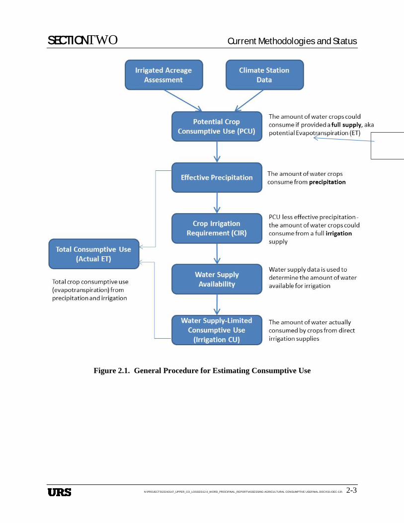
Potential Consumptive Use (PCU). The amount of water crops could consume if provided a full supply, also called potential evapotranspiration (potential ET).
Effective Precipitation. The amount of water crops consume from precipitation.
Crop Irrigation Requirement (CIR). Potential consumptive use less effective precipitation. The amount of water crops could consume from a full irrigation supply.
Supply-limited Consumptive Use (irrigation CU). The amount of water actually consumed by crops from direct irrigation supplies. This term takes into account that the crop may not get a full water supply; therefore irrigation CU will be less than or equal to CIR.
Actual Evapotranspiration (actual ET). The amount of water consumed by crops from all water sources; effective precipitation plus irrigation CU.
In the Consumptive Uses and Losses Report, the term crop consumptive use is used in lieu of the term evapotranspiration. However, in the technical literature associated with remote sensing, the term evapotranspiration is more commonly used.
Figure 2-1 shows the general procedure and data requirements for estimating irrigation CU.
• PCU is calculated based on irrigated acreage information, including crop type, and climate data. Sub-section 2.2 summarizes available irrigated acreage assessments by state, including acreage attributions and frequency of updates.
• Sub-section 2.3 discusses the availability of climate data and the spatial coverage with respect to the location of irrigated acreage in the Upper Basin.
• Sub-section 2.4 discusses different methods used to calculate PCU in the Upper Division States, including method accuracy and data requirements.
• Sub-section 2.5 summarizes effective precipitation methods used to estimate CIR.
• Sub-section 2.6 provides information on water supply data availability.
SECTIONTWO Current Methodologies and Status
N:\PROJECTS\22243147_UPPER_CO_LOSSES\12.0_WORD_PROC\FINAL_REPORT\ASSESSING AGRICULTURAL CONSUMPTIVE USEFINAL.DOCX\31-DEC-13\\ 2-2
• Sub-section 2.7 presents the methods and models used to estimate irrigation CU.
• Sub-section 2.8 presents crop consumptive use models.
SECTIONTWO Current Methodologies and Status
N:\PROJECTS\22243147_UPPER_CO_LOSSES\12.0_WORD_PROC\FINAL_REPORT\ASSESSING AGRICULTURAL CONSUMPTIVE USEFINAL.DOCX\31-DEC-13\\ 2-3
Figure 2.1. General Procedure for Estimating Consumptive Use
SECTIONTWO Current Methodologies and Status
N:\PROJECTS\22243147_UPPER_CO_LOSSES\12.0_WORD_PROC\FINAL_REPORT\ASSESSING AGRICULTURAL CONSUMPTIVE USEFINAL.DOCX\31-DEC-13\\ 2-4
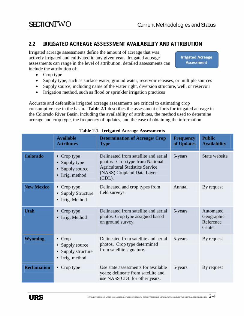
IRRIGATED ACREAGE ASSESSMENT AVAILABILITY AND ATTRIBUTION 2.2Irrigated acreage assessments define the amount of acreage that was actively irrigated and cultivated in any given year. Irrigated acreage assessments can range in the level of attribution; detailed assessments can include the attribution of:
• Crop type • Supply type, such as surface water, ground water, reservoir releases, or multiple sources • Supply source, including name of the water right, diversion structure, well, or reservoir • Irrigation method, such as flood or sprinkler irrigation practices
Accurate and defensible irrigated acreage assessments are critical to estimating crop consumptive use in the basin. Table 2.1 describes the assessment efforts for irrigated acreage in the Colorado River Basin, including the availability of attributes, the method used to determine acreage and crop type, the frequency of updates, and the ease of obtaining the information.
Table 2.1. Irrigated Acreage Assessments Available
Attributes Determination of Acreage/ Crop Type
Frequency of Updates
Public Availability
Colorado • Crop type • Supply type • Supply source • Irrig. method
Delineated from satellite and aerial photos. Crop type from National Agricultural Statistics Service (NASS) Cropland Data Layer (CDL).
5-years State website
New Mexico • Crop type • Supply Structure • Irrig. Method
Delineated and crop types from field surveys.
Annual By request
Utah • Crop type • Irrig. Method
Delineated from satellite and aerial photos. Crop type assigned based on ground survey.
5-years Automated Geographic Reference Center
Wyoming • Crop • Supply source • Supply structure • Irrig. method
Delineated from satellite and aerial photos. Crop type determined from satellite signature.
5-years By request
Reclamation • Crop type Use state assessments for available years; delineate from satellite and use NASS CDL for other years.
5-years By request
SECTIONTWO Current Methodologies and Status
N:\PROJECTS\22243147_UPPER_CO_LOSSES\12.0_WORD_PROC\FINAL_REPORT\ASSESSING AGRICULTURAL CONSUMPTIVE USEFINAL.DOCX\31-DEC-13\\ 2-5
CLIMATE STATION DATA AVAILABILITY 2.3Climate data serves as the basis for estimating the amount of water needed by a crop; climate data availability can be assessed in terms of:
• Spatial Distribution - is there a sufficient distribution of climate stations in proximity to irrigated acreage in the basin to accurately measure the climatic conditions experienced by the acreage?
• Climate Data Measured - what types of climatic factors (e.g., precipitation, wind speed, solar radiation) are recorded at each station?
Understanding the distribution and types of climate data in each state is important because different consumptive use calculation methods require different climate data information; and significant distance between the irrigated acreage and the climate station produces less accurate consumptive use estimates.
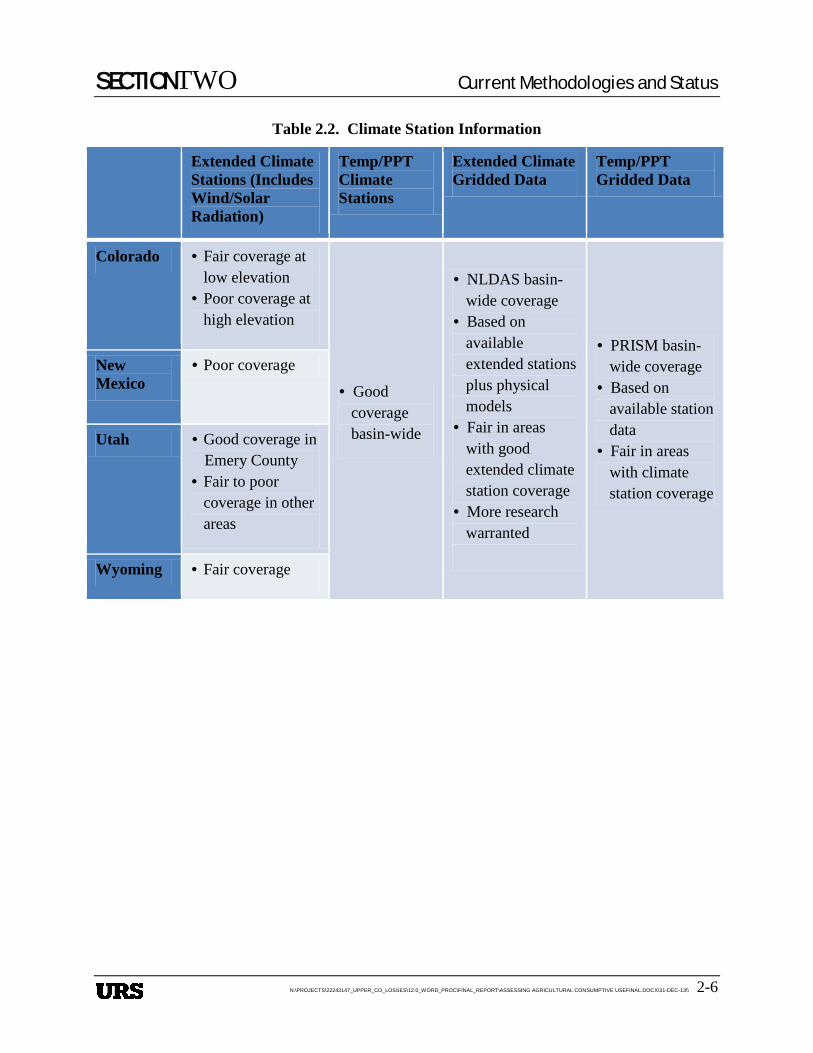
For purposes of this study, climate stations are categorized based on the types of data measured. Stations recording temperature and precipitation only are termed “temperature/precipitation” stations. Stations that record temperature and precipitation plus relative humidity, sky/cloud cover, solar radiation, wind speed and direction, and barometric pressure readings are termed “extended climate” stations.
In addition to tabular climate data, the available format for data at each climate station, climate information can also be processed and distributed in a grid format. There are programs that provide grid-based climate data for the entire Colorado River Basin. Temperature/Precipitation climate grids are available through the Parameter-elevation Regressions on Independent Slopes Model (PRISM) Climate Group program. Five-kilometer gridded extended climate data is available through the North America Land Data Assimilation System (NLDAS). One-kilometer gridded extended climate data, with the exception of wind speed, (DAYMET) is available through the Daily Surface Weather and Climatological Summaries. In addition, Wyoming has developed a gridded climate data representing average monthly values.
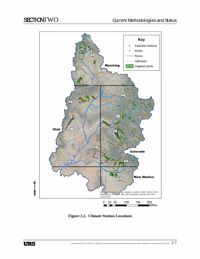
Table 2.2 describes the availability of climate station data in each state. Detailed review of locations of climate stations to determine if they meet stringent siting criteria in terms of surrounding vegetation, adequate fetch to measure wind speed, and other standard criteria was not performed as part of this effort. The qualitative assessment of location coverage in Table 2.2 simply reflects the climate station spacing and proximity to irrigated acreage. Reclamation has access to the climate stations in each state; therefore, a separate entry is not included.
Figure 2.2 shows the location of the National Oceanic and Atmospheric Administration (NOAA) temperature/precipitation and extended climate stations. Also shown on Figure 2.2 is the location of irrigated acreage in the basin.
SECTIONTWO Current Methodologies and Status
N:\PROJECTS\22243147_UPPER_CO_LOSSES\12.0_WORD_PROC\FINAL_REPORT\ASSESSING AGRICULTURAL CONSUMPTIVE USEFINAL.DOCX\31-DEC-13\\ 2-6
Table 2.2. Climate Station Information
Extended Climate Stations (Includes Wind/Solar Radiation)
Temp/PPT Climate Stations
Extended Climate Gridded Data
Temp/PPT Gridded Data
Colorado • Fair coverage at low elevation
• Poor coverage at high elevation
• Good coverage basin-wide
• NLDAS basin-wide coverage
• Based on available extended stations plus physical models
• Fair in areas with good extended climate station coverage
• More research warranted
• PRISM basin-wide coverage
• Based on available station data
• Fair in areas with climate station coverage
New Mexico
• Poor coverage
Utah • Good coverage in Emery County
• Fair to poor coverage in other areas
Wyoming • Fair coverage
SECTIONTWO Current Methodologies and Status
N:\PROJECTS\22243147_UPPER_CO_LOSSES\12.0_WORD_PROC\FINAL_REPORT\ASSESSING AGRICULTURAL CONSUMPTIVE USEFINAL.DOCX\31-DEC-13\\ 2-7
Figure 2.2. Climate Station Locations
SECTIONTWO Current Methodologies and Status
N:\PROJECTS\22243147_UPPER_CO_LOSSES\12.0_WORD_PROC\FINAL_REPORT\ASSESSING AGRICULTURAL CONSUMPTIVE USEFINAL.DOCX\31-DEC-13\\ 2-8
POTENTIAL CROP CONSUMPTIVE USE METHODS 2.4There are several methodologies that estimate PCU, or the amount of water that would be used for crop growth if provided with an ample water supply. They range in complexity, accuracy, and data requirements. Historically, the availability of extended climate data limited the methods used in the Upper Colorado River Basin to methods that relied on readily available temperature data. In some areas of the basin, as discussed in Table 2.2, the lack of extended climate data continues to drive the PCU calculation method employed.
Most of the states and Reclamation have relied on the monthly modified Blaney-Criddle method for estimating PCU, which requires only mean temperature data, with full knowledge that this method does not represent crop demands in the Upper Colorado River Basin as accurately as other methods. Consumptive use experts have recommended the use of the daily Penman-Monteith method for many years; however, this method requires the availability of extended climate data. To more accurately estimate PCU in areas without extended climate data, or when longer periods of historical consumptive use estimates are required, the use of elevation adjustments or locally calibrated crop coefficients have been used to some extent.
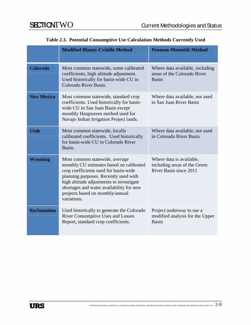
Table 2.3 describes PCU calculation methods currently used in each state and by Reclamation.
SECTIONTWO Current Methodologies and Status
N:\PROJECTS\22243147_UPPER_CO_LOSSES\12.0_WORD_PROC\FINAL_REPORT\ASSESSING AGRICULTURAL CONSUMPTIVE USEFINAL.DOCX\31-DEC-13\\ 2-9
Table 2.3. Potential Consumptive Use Calculation Methods Currently Used
Modified Blaney-Criddle Method Penman-Monteith Method
Colorado Most common statewide, some calibrated coefficients, high altitude adjustment. Used historically for basin-wide CU in Colorado River Basin.
Where data available, including areas of the Colorado River Basin
New Mexico Most common statewide, standard crop coefficients. Used historically for basin-wide CU in San Juan Basin except monthly Hargreaves method used for Navajo Indian Irrigation Project lands.
Where data available, not used in San Juan River Basin
Utah Most common statewide, locally calibrated coefficients. Used historically for basin-wide CU in Colorado River Basin.
Where data available, not used in Colorado River Basin
Wyoming Most common statewide, average monthly CU estimates based on calibrated crop coefficients used for basin-wide planning purposes. Recently used with high altitude adjustments to investigate shortages and water availability for new projects based on monthly/annual variations.
Where data is available, including areas of the Green River Basin since 2011
Reclamation Used historically to generate the Colorado River Consumptive Uses and Losses Report, standard crop coefficients.
Project underway to use a modified analysis for the Upper Basin
SECTIONTWO Current Methodologies and Status
N:\PROJECTS\22243147_UPPER_CO_LOSSES\12.0_WORD_PROC\FINAL_REPORT\ASSESSING AGRICULTURAL CONSUMPTIVE USEFINAL.DOCX\31-DEC-13\\ 2-10
EFFECTIVE PRECIPITATION ESTIMATION 2.5METHODS Effective precipitation is the amount of precipitation during the irrigation season that is effective in satisfying a portion of PCU. Effective precipitation is used to estimate that amount of water crops could consume from a full irrigation supply. Crop irrigation requirement is calculated as PCU less effective precipitation. Estimating effective precipitation is also critical if a remote sensing method is used to determine irrigation CU for future consumptive uses and losses reporting, as the Upper Basin states are required to report diversion-caused depletions only.
At this time, each of the states (with the exception of Utah) and Reclamation rely on the SCS monthly method outlined in Technical Release 21 in the Colorado River Basin. Utah estimates effective precipitation to be 80 percent of total precipitation during the irrigation season.
WATER SUPPLY DATA AVAILABILITY 2.6Climate data, crop type, and acreage amounts are used to estimate the PCU; water supply data is used to determine the irrigation CU.
The need to administer water rights and permits, and the agency responsible varies by state. In each state, there are tributaries with limited supply that require regulation or administration to ensure senior water rights can divert. In Wyoming and Colorado, administration requires measurement of headgate diversions. In Utah and New Mexico, headgate diversions may be measured, but often stream flows are used to determine water availability by water right priority.
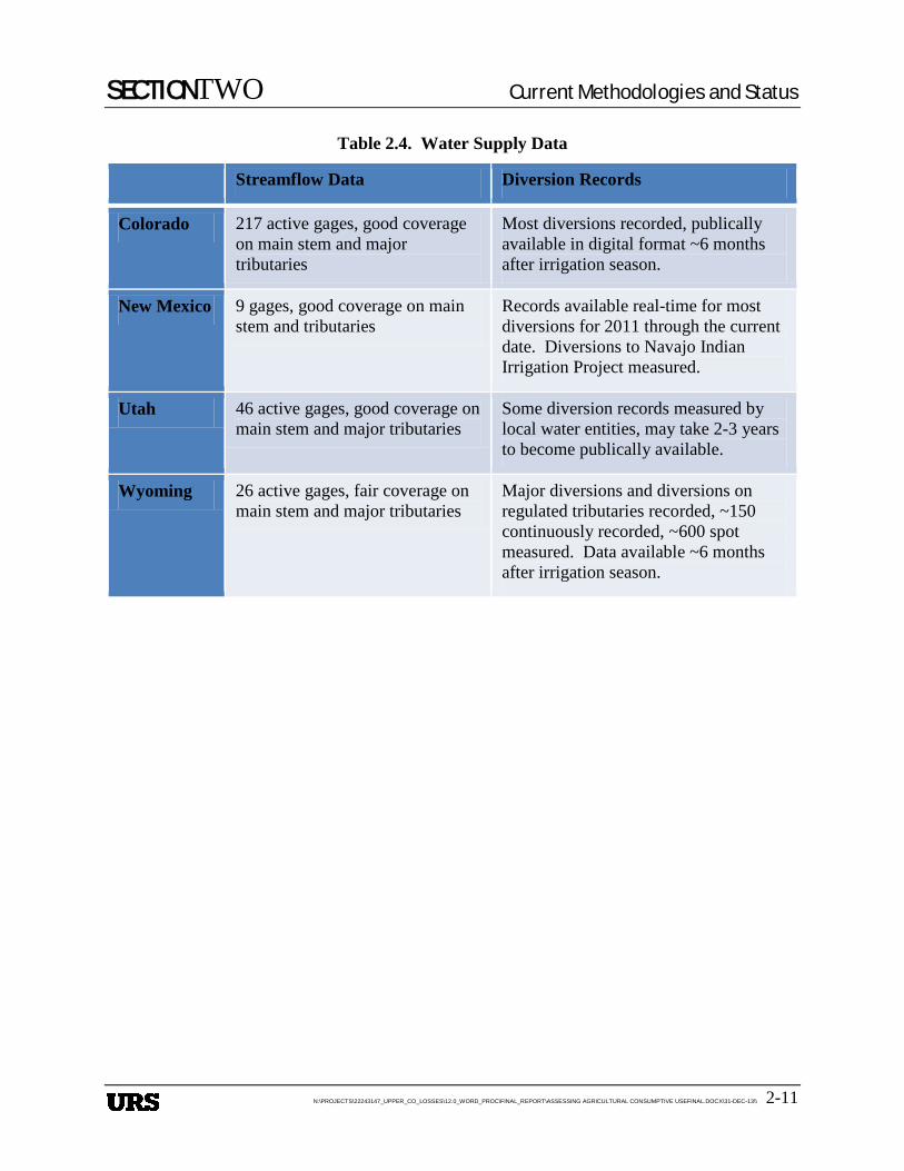
For the purposes of this study, active streamflow gages and river headgate diversion records were reviewed. Table 2.4 describes existing state water supply data, including the availability of active gages and diversions, locations, quality of coverage, and ease of obtaining the data. Reclamation has access to the stream gages in each state; therefore, a separate entry is not included. Reclamation does not maintain diversion records in the Upper Basin States.
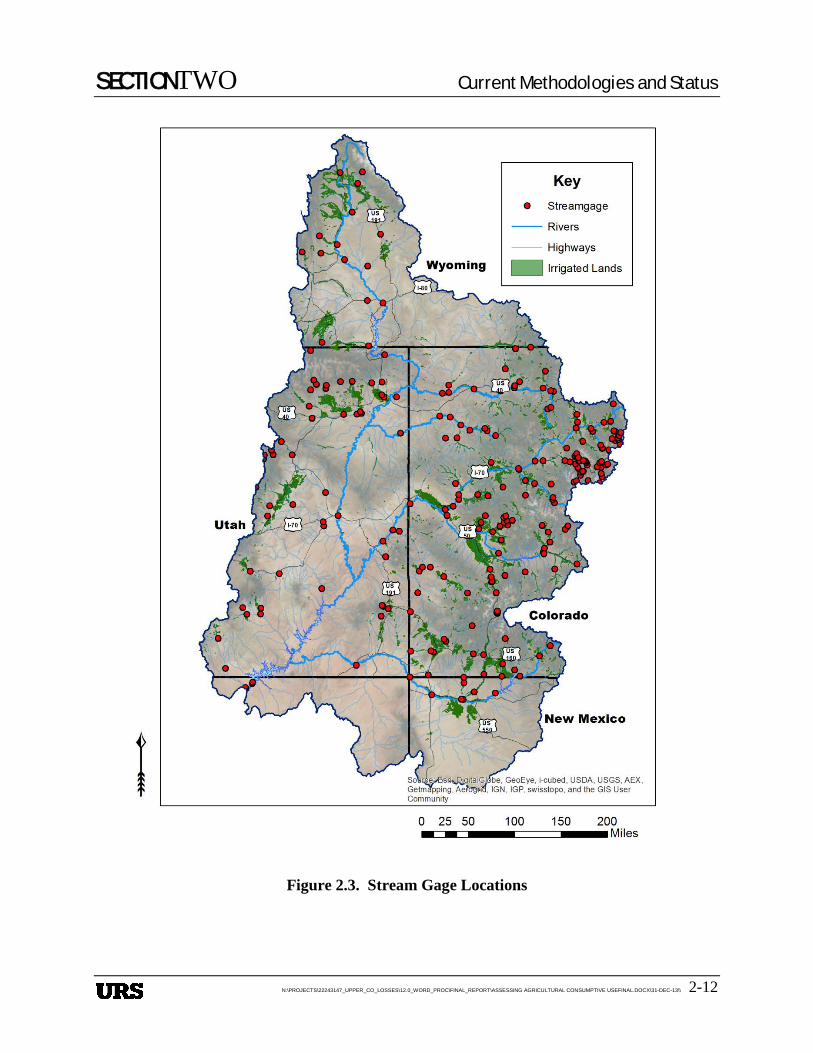
Figure 2.3 shows the location of stream gages in the basin.
SECTIONTWO Current Methodologies and Status
N:\PROJECTS\22243147_UPPER_CO_LOSSES\12.0_WORD_PROC\FINAL_REPORT\ASSESSING AGRICULTURAL CONSUMPTIVE USEFINAL.DOCX\31-DEC-13\\ 2-11
Table 2.4. Water Supply Data
Streamflow Data Diversion Records
Colorado 217 active gages, good coverage on main stem and major tributaries
Most diversions recorded, publically available in digital format ~6 months after irrigation season.
New Mexico 9 gages, good coverage on main stem and tributaries
Records available real-time for most diversions for 2011 through the current date. Diversions to Navajo Indian Irrigation Project measured.
Utah 46 active gages, good coverage on main stem and major tributaries
Some diversion records measured by local water entities, may take 2-3 years to become publically available.
Wyoming 26 active gages, fair coverage on main stem and major tributaries
Major diversions and diversions on regulated tributaries recorded, ~150 continuously recorded, ~600 spot measured. Data available ~6 months after irrigation season.
SECTIONTWO Current Methodologies and Status
N:\PROJECTS\22243147_UPPER_CO_LOSSES\12.0_WORD_PROC\FINAL_REPORT\ASSESSING AGRICULTURAL CONSUMPTIVE USEFINAL.DOCX\31-DEC-13\\ 2-12
Figure 2.3. Stream Gage Locations
SECTIONTWO Current Methodologies and Status
N:\PROJECTS\22243147_UPPER_CO_LOSSES\12.0_WORD_PROC\FINAL_REPORT\ASSESSING AGRICULTURAL CONSUMPTIVE USEFINAL.DOCX\31-DEC-13\\ 2-13
WATER SUPPLY-LIMITED CONSUMPTIVE USE CALCULATION METHODS 2.7There are several methods used by the states and Reclamation to calculate irrigation CU. The most detailed method uses diversion records to perform an on-farm water balance, comparing CIR to water supply, resulting in irrigation CU. Other methods used in areas where diversion records are unavailable rely on measured streamflow data to estimate irrigation CU. Utah determines supply limitations by sub-basin using an inflow-outflow method that considers available measured and estimated data to determine supply limitations. Reclamation uses an indicator gage approach that ties water available for irrigation to streamflow at nearby stream gages. Remote sensing methods have been used to measure total consumptive use (actual ET) on a more local scale both by the individual states by Reclamation.
Table 2-5 highlights both the methods each state and Reclamation use to estimate irrigation CU, and the specific models used, as discussed in the next sub-section.
CROP CONSUMPTIVE USE MODELS 2.8There are several models used in the states and by Reclamation to estimate PCU and CIR based on climate data, acreage data, and crop type. Some models also include methods to estimate irrigation CU. Models used to estimate irrigation CU take varying approaches. The most detailed method uses diversion records to perform an on-farm water balance, comparing CIR to water supply, resulting in irrigation CU. Other methods used in areas where diversion records are unavailable rely on measured streamflow data to estimate water supply availability and irrigation CU. As discussed in more detail in Section 3, remote sensing models measure irrigation CU directly.
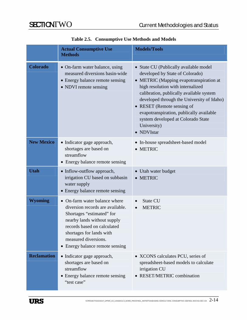
Table 2.5 describes the methods used in each state and by Reclamation to estimate irrigation CU and specific modeling tools used. Table 2.5 highlights that remote sensing has been used to varying extents in each of the Upper Basin states. In general, the states update their consumptive use analyses to coincide with irrigated acreage assessments. Reclamation updates the consumptive use analysis for the Consumptive Uses and Losses Report annually on a provisional basis. Finalization can take several years. Section 3 provides detail on the current status and future opportunities of remote sensing.
SECTIONTWO Current Methodologies and Status
N:\PROJECTS\22243147_UPPER_CO_LOSSES\12.0_WORD_PROC\FINAL_REPORT\ASSESSING AGRICULTURAL CONSUMPTIVE USEFINAL.DOCX\31-DEC-13\\ 2-14
Table 2.5. Consumptive Use Methods and Models
Actual Consumptive Use Methods
Models/Tools
Colorado • On-farm water balance, using measured diversions basin-wide
• Energy balance remote sensing • NDVI remote sensing
• State CU (Publically available model developed by State of Colorado)
• METRIC (Mapping evapotranspiration at high resolution with internalized calibration, publically available system developed through the University of Idaho)
• RESET (Remote sensing of evapotranspiration, publically available system developed at Colorado State University)
• NDVIstar
New Mexico • Indicator gage approach, shortages are based on streamflow
• Energy balance remote sensing
• In-house spreadsheet-based model • METRIC
Utah • Inflow-outflow approach, irrigation CU based on subbasin water supply
• Energy balance remote sensing
• Utah water budget • METRIC
Wyoming • On-farm water balance where diversion records are available. Shortages “estimated” for nearby lands without supply records based on calculated shortages for lands with measured diversions.
• Energy balance remote sensing
• State CU • METRIC
Reclamation • Indicator gage approach, shortages are based on streamflow
• Energy balance remote sensing “test case”
• XCONS calculates PCU, series of spreadsheet-based models to calculate irrigation CU
• RESET/METRIC combination
SECTIONTHREE Potential Applicable Methodologies
N:\PROJECTS\22243147_UPPER_CO_LOSSES\12.0_WORD_PROC\FINAL_REPORT\ASSESSING AGRICULTURAL CONSUMPTIVE USEFINAL.DOCX\31-DEC-13\\ 3-1
3. Section 3 THR EE Potential Applicable M ethodologies
POTENTIAL APPLICATION OF REMOTE SENSING METHODS 3.1Remote sensing methods provide information on total consumptive use (actual ET) over large spatial areas at relatively frequent intervals. Because they measure actual use from both precipitation and irrigation, they may have advantages over traditional methods that estimate potential consumptive use based on empirical data and then rely on measurements or estimates of water availability to determine actual ET. Remote sensing methods are being considered as an alternative to traditional methods largely due to their potential for accurately representing basin consumptive use, their large-scale geographic applicability, their non-reliance on water supply information, and their potential for relatively rapid processing. It should be noted that these techniques currently present a number of implementation challenges including the need to fill data between satellite overpasses, the very large spatial area for processing, and the requirement for ground-based verification/calibration.
Water use data for the Consumptive Uses and Losses Report reflects depletions from irrigation supplies only (irrigation CU). Because remote sensing methods measure actual ET from both precipitation (natural) and irrigation water sources, effective precipitation estimates need to be removed from remote sensing actual ET estimates to determine irrigation CU.
3.1.1 Background and Objectives The objective of this section of the report is to describe potential application of remotely sensed spectral reflectance data in various wavelengths to the calculation of actual ET of vegetated surfaces, particularly irrigated surfaces, in the Upper Colorado River Basin states. The first step is the calculation of the instantaneous evaporative flux of the vegetative surface under observation at the time of satellite overpass using a radiation and energy balance approach. These instantaneous fluxes need to be converted to daily and then seasonal fluxes to determine the evapotranspiration of the vegetated surface for the complete growing season.
This project investigates the practicality of application of remotely sensed data to estimate consumptive use by irrigated agriculture in this region. It presents a sample application of remotely sensed data for this use and indicates other approaches that have been used or are being developed. The expected accuracy of this approach based on previous studies is also discussed. Recommendations are made for the definition of a potential remote sensing platform and acquisition of remote sensing data, collection of satellite data and additional supporting meteorological data required for efficient computation of actual ET using remote sensing. This report also addresses the following elements:
• Higher elevation crop growth
• Areas with significant variations in elevation over satellite scenes
• Application of cold water to crops
• Separation of irrigated crops from other vegetation
• Availability of ground-based climate data for calibration
• Required number of images for each irrigation season
SECTIONTHREE Potential Applicable Methodologies
N:\PROJECTS\22243147_UPPER_CO_LOSSES\12.0_WORD_PROC\FINAL_REPORT\ASSESSING AGRICULTURAL CONSUMPTIVE USEFINAL.DOCX\31-DEC-13\\ 3-2
• Interpolation of data between available scenes
• Satellite images with cloud cover
• Crop cutting between satellite images
3.1.2 Review of Traditional and Ground-Based Consumptive Use Estimating Methods Prior to evaluating actual ET estimating methods that are based on remotely sensed data, it is helpful to understand the range of traditional and ground-based methods that are available and the relative accuracies of each. Some of these methods are combined with remote sensing data processing procedures and some are used to ground truth and validate remotely sensed estimates.
As described in Section 2, a number of different methods are employed in different states to estimate the potential consumptive water use of crops, effective precipitation, crop irrigation requirements, and the actual CU. These differences are in part generated by the availability of meteorological data, including solar radiation, wind speed, and relative humidity, in addition to the standard parameters of minimum and maximum temperature and precipitation. The distribution of temperature and precipitation stations is judged as good throughout the Upper Colorado River Basin. The additional data required to make a more sophisticated evaluation of potential crop water use, e.g., using the Penman-Monteith method (Allen et al., 1998; Allen et al., 2005), vary from poor to fair coverage depending on location. These results are summarized in Table 3.1.
As discussed in Section 2, the most common method for computing potential crop water use in the four states is the modified Blaney-Criddle method, a temperature-based method that generally uses seasonal crop coefficients. This method is applied in Wyoming with some high-altitude adjustment, in Colorado with high-altitude adjustment and some locally calibrated crop coefficients, in Utah with some locally calibrated crop coefficients, and in New Mexico where the Hargreaves method (also temperature-based) is used on Navajo Indian Irrigation Project (NIIP) lands. The more sophisticated Penman-Monteith method is used in select basins in all four states where adequate data are available. These results are summarized in Table 3.2.
It is worthwhile to compare the accuracy of the PCU methods used in the Upper Colorado River Basin that have fewer data requirements than the Penman-Monteith method. Both the modified Blaney-Criddle and Hargreaves methods are temperature-based methods and air temperature is the basic data requirement. These methods also have a minimum recommended time of application based on the original calibration of the method (Jensen et al., 1990). The minimum recommended time of application for the modified Blaney-Criddle method is monthly if local calibration coefficients are derived (seasonal if there are no local calibration coefficients. The minimum recommended time of application for the Hargreaves method is 10 days. These recommendations contrast with the Penman-Monteith method, for which the minimum time period of application is daily. The data requirements for the Penman-Monteith method, in addition to air temperature, are solar radiation, relative humidity, and wind speed.
Common ground-based methods for determining actual ET include use of a weighing lysimeter, the Bowen ratio-energy balance (BREB) approach (Bowen, 1926), and the eddy covariance technique (EC). Use of the scintillometer device is another approach to determine actual ET over fields, but recent work indicates problems with this method (Kleissl et al., 2008; Kleissl et al., 2009). Of the commonly applied methods, only a precise weighing lysimeter can be
SECTIONTHREE Potential Applicable Methodologies
N:\PROJECTS\22243147_UPPER_CO_LOSSES\12.0_WORD_PROC\FINAL_REPORT\ASSESSING AGRICULTURAL CONSUMPTIVE USEFINAL.DOCX\31-DEC-13\\ 3-3
considered to be free from assumptions about the physics of the system and can therefore be used as “ground truth” to evaluate other methods. However, installation costs for precise weighing lysimeters are tens of thousands of dollars and additional funding is required for operation. For this reason there are only a handful of precise weighing lysimeter sites in North America and indeed worldwide.
Table 3.3 indicates the comparison of the estimating methods with 13 precise weighing lysimeters from around the world, based on Jensen et al., (1990). The weighing lysimeters were provided a full irrigation supply; therefore, the instruments were able to measure PCU. Results are given for average peak month PCU compared to lysimeter-measured PCU (percent), seasonal PCU estimates compared to that measured by the lysimeter (percent), and the standard error of the estimate compared to the lysimeter (mm/d). The results are divided into arid and humid lysimeter sites, with the arid sites being more representative of conditions in the Upper Colorado River Basin. As shown, average peak month PCU tends to be underestimated by 14 percent using the modified Blaney-Criddle method, underestimated by 12 percent using the Hargreaves method, and underestimated by 4 percent using the Penman-Monteith method. Seasonal PCU estimates indicate a similar pattern with the Penman-Monteith method equaling 99 percent of measured PCU. Also the standard error of the estimate of the Penman-Monteith method is one-third to one-half that of the other two methods.
3.1.3 Factors Affecting Actual Crop Evapotranspiration Various conditions on the ground can cause actual ET to be less than PCU. These include lack of adequate root zone soil moisture due to limited water supply, effects of soil salinity levels, lack of aeration of the root zone due to over-irrigation, and plant disease. All of these conditions cause plant stress which generally causes increased plant stomatal resistance and reduced evapotranspiration. The reduction of ET causes a yield reduction below maximum yield, which is a function of the yield reduction ratio (i.e., drought tolerance) of the plant (Cuenca, 1989).
Other factors that affect actual ET and crop production include plant density below the recommended values, uneven distribution of surface and sprinkler irrigation applications, emitter clogging in drip irrigation systems, lack of adequate soil fertility, and poor timing (i.e., management) of irrigation applications. All of these factors cause actual ET to be below PCU. Any “ET index” approach, including a crop coefficient approach that does not account for all of the above factors, will produce unrealistic, generally high, estimates of actual ET. The effects indicated can at times be at a relatively small scale, i.e., less than field scale. This is true for most of the factors, but particularly for irrigation systems with less than acceptable levels of uniformity of application.
Consumptive uses and losses reporting in the Upper Colorado River Basin requires an assessment of actual CU across each state and sub-basin with sometimes widely different water and crop management conditions. Measurement of water availability varies across the Upper Basin, making it difficult to use water supply methods to estimate actual CU. One of the primary reasons for evaluating remote sensing methodologies for use in consumptive uses and losses reporting is the ability to remotely assess actual CU down to a field and basin scale without the need to have water supply and irrigation practice information.
SECTIONTHREE Potential Applicable Methodologies
N:\PROJECTS\22243147_UPPER_CO_LOSSES\12.0_WORD_PROC\FINAL_REPORT\ASSESSING AGRICULTURAL CONSUMPTIVE USEFINAL.DOCX\31-DEC-13\\ 3-4
3.1.4 Resolution Issues Related to Irrigated Agriculture Due to the factors affecting actual ET listed in sub-section 3.1.3, it is easy to understand the need to evaluate evapotranspiration on at least a field scale, e.g., tens of meters, if not a sub-field scale. The spatial resolution of a subset of current satellite platforms will be described later. However, discussion of the resolution issue related to irrigated agriculture in this sub-section will focus on Landsat with a thermal band resolution of 60- to 100-m contrasted with the MODIS (Moderate Resolution Imaging Spectroradiometer) system with a thermal band resolution of 1,000-m. Figure 3.1 indicates a direct contrast of a scene from Google Earth in the San Joaquin Valley of California with an ET retrieval from the MODIS platform for exactly the same area. It is clear that the features of the individual fields are completely washed out in the MODIS product and it is not possible to discern individual field boundaries.
Figure 3.2 shows a Landsat scene for the Paraná River Delta in South America at the same resolution as that for retrieval of crop ET using Landsat data. The image on the left shows part of the Paraná River and an irrigated sector in the lower left of the image. The image on the right is taken from zooming in on the irrigated area within the red box. The individual farm fields in different stages of growth and crop response to irrigation are quite distinct. It can then be argued that something on the order of the spatial resolution of Landsat data would be acceptable for evaluation of irrigation in the Upper Colorado River Basin.
A further example is indicated on Figures 3.3 (a) and (b). This is a normalized difference vegetation index (NDVI) scene (computed using red and near infrared reflectance) of the Wood River Valley in southern Oregon using Landsat data. Figure 3.3 (a) is of the entire valley with a scale of 10 km indicated. Figure 3.3 (b) is a pixelated view of the area at the center of Figure 3.3 (a) indicating the 30-m resolution of the visible and near infrared sensors of the Landsat satellites.
RADIATION AND ENERGY BALANCE TERMINOLOGY AND CONCEPTS 3.2The fundamental physics used to estimate actual ET from a combination of remotely sensed spectral reflectance data and ground based meteorological data centers around the calculation of radiation and energy balances at the Earth’s surface. Although there are a multitude of different satellite platforms available to provide remotely sensed images of the Earth’s surface, only certain platforms possess the spectral sensing capabilities needed to support the full radiation and energy balance. This sub-section briefly reviews these issues to provide the reader with an overview of the basic processes used in calculating actual ET at the time of a single satellite image.
3.2.1 Components of the Radiation Balance This sub-section describes the basic components required to compute the radiation balance, which is the first step in computing the energy balance. The explanation of equations applied for the radiation balance is simplified. For a complete listing of the steps, equations, and bands required to make the calculations using remote sensing data, refer to Eckhardt (2013).
Wein’s displacement law requires that radiation emanating from the Sun (solar radiation) will be centered around a relatively short wavelength and radiation emanating from the Earth (terrestrial
SECTIONTHREE Potential Applicable Methodologies
N:\PROJECTS\22243147_UPPER_CO_LOSSES\12.0_WORD_PROC\FINAL_REPORT\ASSESSING AGRICULTURAL CONSUMPTIVE USEFINAL.DOCX\31-DEC-13\\ 3-5
radiation) will be centered around a relatively long wavelength. Solar radiation is therefore referred to as shortwave radiation while terrestrial radiation is termed longwave radiation.
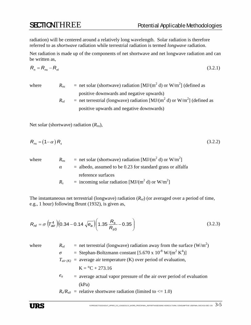
Net radiation is made up of the components of net shortwave and net longwave radiation and can be written as,
n ns nlR R R= − (3.2.1)
where Rns = net solar (shortwave) radiation [MJ/(m2 d) or W/m2] (defined as
positive downwards and negative upwards) Rnl = net terrestrial (longwave) radiation [MJ/(m2 d) or W/m2] (defined as
positive upwards and negative downwards)
Net solar (shortwave) radiation (Rns),
( )1ns sR Rα= − (3.2.2)
where Rns = net solar (shortwave) radiation [MJ/(m2 d) or W/m2] α = albedo, assumed to be 0.23 for standard grass or alfalfa
reference surfaces Rs = incoming solar radiation [MJ/(m2 d) or W/m2]
The instantaneous net terrestrial (longwave) radiation (Rnl) (or averaged over a period of time, e.g., 1 hour) following Brunt (1932), is given as,
( ) ( )
−−= 35.035.114.034.0
0
4
s
saairnl R
ReTR σ (3.2.3)
where Rnl = net terrestrial (longwave) radiation away from the surface (W/m2) σ = Stephan-Boltzmann constant [5.670 x 10⁻⁸ W/(m2 K4)] Tair (K) = average air temperature (K) over period of evaluation,
K = °C + 273.16 ea = average actual vapor pressure of the air over period of evaluation
(kPa) Rs/Rs0 = relative shortwave radiation (limited to <= 1.0)
SECTIONTHREE Potential Applicable Methodologies
N:\PROJECTS\22243147_UPPER_CO_LOSSES\12.0_WORD_PROC\FINAL_REPORT\ASSESSING AGRICULTURAL CONSUMPTIVE USEFINAL.DOCX\31-DEC-13\\ 3-6
Rs = average incoming solar radiation over period of evaluation (W/m2) Rs0 = average clear-sky solar radiation over period of evaluation (W/m2)
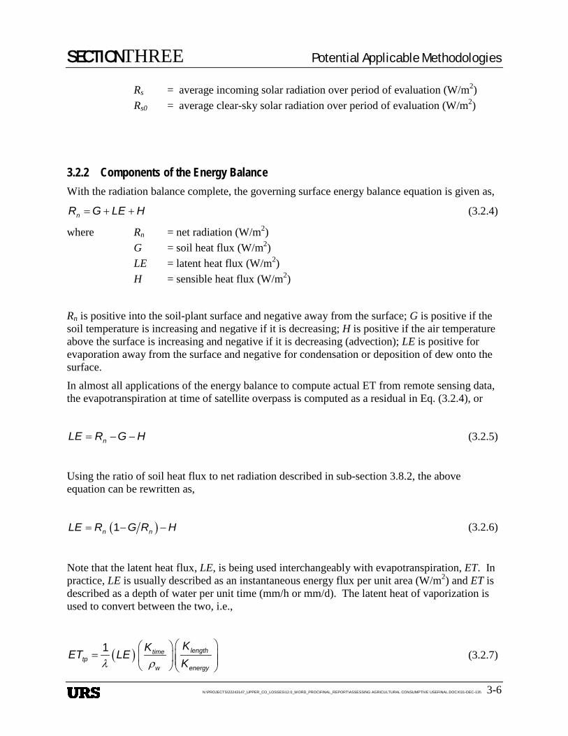
3.2.2 Components of the Energy Balance With the radiation balance complete, the governing surface energy balance equation is given as,
= + +nR G LE H (3.2.4)
where Rn = net radiation (W/m2) G = soil heat flux (W/m2)
LE = latent heat flux (W/m2) H = sensible heat flux (W/m2)
Rn is positive into the soil-plant surface and negative away from the surface; G is positive if the soil temperature is increasing and negative if it is decreasing; H is positive if the air temperature above the surface is increasing and negative if it is decreasing (advection); LE is positive for evaporation away from the surface and negative for condensation or deposition of dew onto the surface.
In almost all applications of the energy balance to compute actual ET from remote sensing data, the evapotranspiration at time of satellite overpass is computed as a residual in Eq. (3.2.4), or
= − −nLE R G H (3.2.5)
Using the ratio of soil heat flux to net radiation described in sub-section 3.8.2, the above equation can be rewritten as,
( )= − −1n nLE R G R H (3.2.6)
Note that the latent heat flux, LE, is being used interchangeably with evapotranspiration, ET. In practice, LE is usually described as an instantaneous energy flux per unit area (W/m2) and ET is described as a depth of water per unit time (mm/h or mm/d). The latent heat of vaporization is used to convert between the two, i.e.,
( )λ ρ
=
1 lengthtimetp
w energy
KKET LEK
(3.2.7)
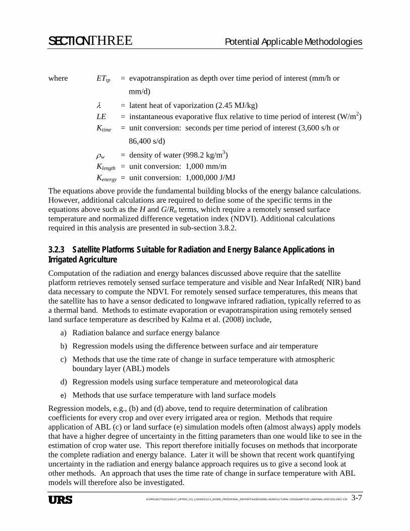
SECTIONTHREE Potential Applicable Methodologies
N:\PROJECTS\22243147_UPPER_CO_LOSSES\12.0_WORD_PROC\FINAL_REPORT\ASSESSING AGRICULTURAL CONSUMPTIVE USEFINAL.DOCX\31-DEC-13\\ 3-7
where ETtp = evapotranspiration as depth over time period of interest (mm/h or
mm/d)
λ = latent heat of vaporization (2.45 MJ/kg) LE = instantaneous evaporative flux relative to time period of interest (W/m2) Ktime = unit conversion: seconds per time period of interest (3,600 s/h or
86,400 s/d)
ρw = density of water (998.2 kg/m3) Klength = unit conversion: 1,000 mm/m Kenergy = unit conversion: 1,000,000 J/MJ
The equations above provide the fundamental building blocks of the energy balance calculations. However, additional calculations are required to define some of the specific terms in the equations above such as the H and G/Rn terms, which require a remotely sensed surface temperature and normalized difference vegetation index (NDVI). Additional calculations required in this analysis are presented in sub-section 3.8.2.
3.2.3 Satellite Platforms Suitable for Radiation and Energy Balance Applications in Irrigated Agriculture Computation of the radiation and energy balances discussed above require that the satellite platform retrieves remotely sensed surface temperature and visible and Near InfaRed( NIR) band data necessary to compute the NDVI. For remotely sensed surface temperatures, this means that the satellite has to have a sensor dedicated to longwave infrared radiation, typically referred to as a thermal band. Methods to estimate evaporation or evapotranspiration using remotely sensed land surface temperature as described by Kalma et al. (2008) include,
a) Radiation balance and surface energy balance
b) Regression models using the difference between surface and air temperature
c) Methods that use the time rate of change in surface temperature with atmospheric boundary layer (ABL) models
d) Regression models using surface temperature and meteorological data
e) Methods that use surface temperature with land surface models
Regression models, e.g., (b) and (d) above, tend to require determination of calibration coefficients for every crop and over every irrigated area or region. Methods that require application of ABL (c) or land surface (e) simulation models often (almost always) apply models that have a higher degree of uncertainty in the fitting parameters than one would like to see in the estimation of crop water use. This report therefore initially focuses on methods that incorporate the complete radiation and energy balance. Later it will be shown that recent work quantifying uncertainty in the radiation and energy balance approach requires us to give a second look at other methods. An approach that uses the time rate of change in surface temperature with ABL models will therefore also be investigated.
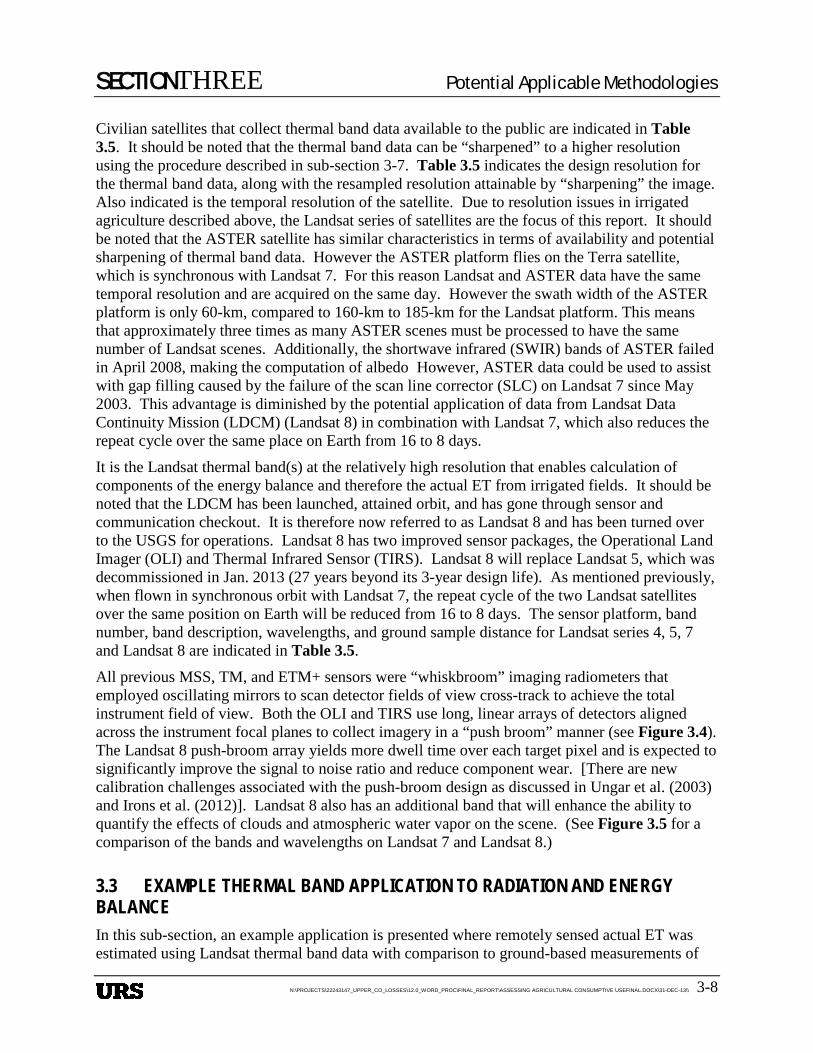
SECTIONTHREE Potential Applicable Methodologies
N:\PROJECTS\22243147_UPPER_CO_LOSSES\12.0_WORD_PROC\FINAL_REPORT\ASSESSING AGRICULTURAL CONSUMPTIVE USEFINAL.DOCX\31-DEC-13\\ 3-8
Civilian satellites that collect thermal band data available to the public are indicated in Table 3.5. It should be noted that the thermal band data can be “sharpened” to a higher resolution using the procedure described in sub-section 3-7. Table 3.5 indicates the design resolution for the thermal band data, along with the resampled resolution attainable by “sharpening” the image. Also indicated is the temporal resolution of the satellite. Due to resolution issues in irrigated agriculture described above, the Landsat series of satellites are the focus of this report. It should be noted that the ASTER satellite has similar characteristics in terms of availability and potential sharpening of thermal band data. However the ASTER platform flies on the Terra satellite, which is synchronous with Landsat 7. For this reason Landsat and ASTER data have the same temporal resolution and are acquired on the same day. However the swath width of the ASTER platform is only 60-km, compared to 160-km to 185-km for the Landsat platform. This means that approximately three times as many ASTER scenes must be processed to have the same number of Landsat scenes. Additionally, the shortwave infrared (SWIR) bands of ASTER failed in April 2008, making the computation of albedo However, ASTER data could be used to assist with gap filling caused by the failure of the scan line corrector (SLC) on Landsat 7 since May 2003. This advantage is diminished by the potential application of data from Landsat Data Continuity Mission (LDCM) (Landsat 8) in combination with Landsat 7, which also reduces the repeat cycle over the same place on Earth from 16 to 8 days.
It is the Landsat thermal band(s) at the relatively high resolution that enables calculation of components of the energy balance and therefore the actual ET from irrigated fields. It should be noted that the LDCM has been launched, attained orbit, and has gone through sensor and communication checkout. It is therefore now referred to as Landsat 8 and has been turned over to the USGS for operations. Landsat 8 has two improved sensor packages, the Operational Land Imager (OLI) and Thermal Infrared Sensor (TIRS). Landsat 8 will replace Landsat 5, which was decommissioned in Jan. 2013 (27 years beyond its 3-year design life). As mentioned previously, when flown in synchronous orbit with Landsat 7, the repeat cycle of the two Landsat satellites over the same position on Earth will be reduced from 16 to 8 days. The sensor platform, band number, band description, wavelengths, and ground sample distance for Landsat series 4, 5, 7 and Landsat 8 are indicated in Table 3.5.
All previous MSS, TM, and ETM+ sensors were “whiskbroom” imaging radiometers that employed oscillating mirrors to scan detector fields of view cross-track to achieve the total instrument field of view. Both the OLI and TIRS use long, linear arrays of detectors aligned across the instrument focal planes to collect imagery in a “push broom” manner (see Figure 3.4). The Landsat 8 push-broom array yields more dwell time over each target pixel and is expected to significantly improve the signal to noise ratio and reduce component wear. [There are new calibration challenges associated with the push-broom design as discussed in Ungar et al. (2003) and Irons et al. (2012)]. Landsat 8 also has an additional band that will enhance the ability to quantify the effects of clouds and atmospheric water vapor on the scene. (See Figure 3.5 for a comparison of the bands and wavelengths on Landsat 7 and Landsat 8.)
EXAMPLE THERMAL BAND APPLICATION TO RADIATION AND ENERGY 3.3BALANCE In this sub-section, an example application is presented where remotely sensed actual ET was estimated using Landsat thermal band data with comparison to ground-based measurements of
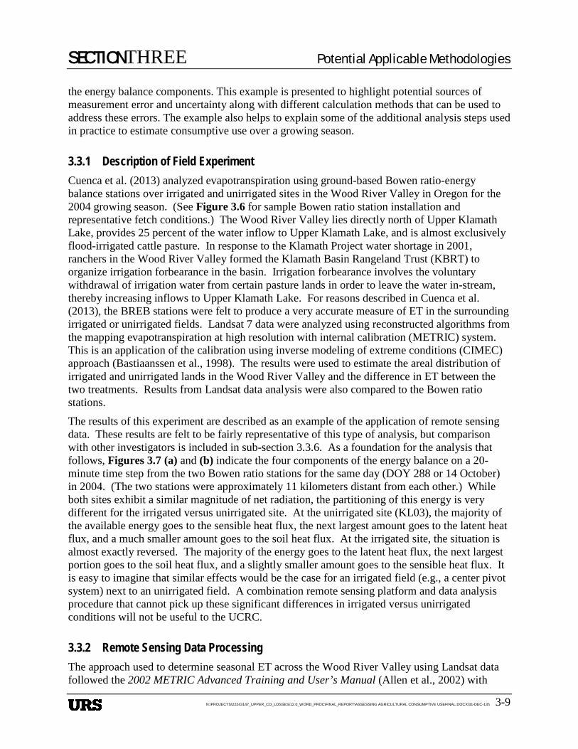
SECTIONTHREE Potential Applicable Methodologies
N:\PROJECTS\22243147_UPPER_CO_LOSSES\12.0_WORD_PROC\FINAL_REPORT\ASSESSING AGRICULTURAL CONSUMPTIVE USEFINAL.DOCX\31-DEC-13\\ 3-9
the energy balance components. This example is presented to highlight potential sources of measurement error and uncertainty along with different calculation methods that can be used to address these errors. The example also helps to explain some of the additional analysis steps used in practice to estimate consumptive use over a growing season.
3.3.1 Description of Field Experiment Cuenca et al. (2013) analyzed evapotranspiration using ground-based Bowen ratio-energy balance stations over irrigated and unirrigated sites in the Wood River Valley in Oregon for the 2004 growing season. (See Figure 3.6 for sample Bowen ratio station installation and representative fetch conditions.) The Wood River Valley lies directly north of Upper Klamath Lake, provides 25 percent of the water inflow to Upper Klamath Lake, and is almost exclusively flood-irrigated cattle pasture. In response to the Klamath Project water shortage in 2001, ranchers in the Wood River Valley formed the Klamath Basin Rangeland Trust (KBRT) to organize irrigation forbearance in the basin. Irrigation forbearance involves the voluntary withdrawal of irrigation water from certain pasture lands in order to leave the water in-stream, thereby increasing inflows to Upper Klamath Lake. For reasons described in Cuenca et al. (2013), the BREB stations were felt to produce a very accurate measure of ET in the surrounding irrigated or unirrigated fields. Landsat 7 data were analyzed using reconstructed algorithms from the mapping evapotranspiration at high resolution with internal calibration (METRIC) system. This is an application of the calibration using inverse modeling of extreme conditions (CIMEC) approach (Bastiaanssen et al., 1998). The results were used to estimate the areal distribution of irrigated and unirrigated lands in the Wood River Valley and the difference in ET between the two treatments. Results from Landsat data analysis were also compared to the Bowen ratio stations.
The results of this experiment are described as an example of the application of remote sensing data. These results are felt to be fairly representative of this type of analysis, but comparison with other investigators is included in sub-section 3.3.6. As a foundation for the analysis that follows, Figures 3.7 (a) and (b) indicate the four components of the energy balance on a 20-minute time step from the two Bowen ratio stations for the same day (DOY 288 or 14 October) in 2004. (The two stations were approximately 11 kilometers distant from each other.) While both sites exhibit a similar magnitude of net radiation, the partitioning of this energy is very different for the irrigated versus unirrigated site. At the unirrigated site (KL03), the majority of the available energy goes to the sensible heat flux, the next largest amount goes to the latent heat flux, and a much smaller amount goes to the soil heat flux. At the irrigated site, the situation is almost exactly reversed. The majority of the energy goes to the latent heat flux, the next largest portion goes to the soil heat flux, and a slightly smaller amount goes to the sensible heat flux. It is easy to imagine that similar effects would be the case for an irrigated field (e.g., a center pivot system) next to an unirrigated field. A combination remote sensing platform and data analysis procedure that cannot pick up these significant differences in irrigated versus unirrigated conditions will not be useful to the UCRC.
3.3.2 Remote Sensing Data Processing The approach used to determine seasonal ET across the Wood River Valley using Landsat data followed the 2002 METRIC Advanced Training and User’s Manual (Allen et al., 2002) with
SECTIONTHREE Potential Applicable Methodologies
N:\PROJECTS\22243147_UPPER_CO_LOSSES\12.0_WORD_PROC\FINAL_REPORT\ASSESSING AGRICULTURAL CONSUMPTIVE USEFINAL.DOCX\31-DEC-13\\ 3-10
ERDAS IMAGINE software. This approach involves solution of the radiation balance as indicated in sub-section 3.2.1, solution of the soil heat flux as indicated in sub-section 3.8.2, iterative solution of the sensible heat flux as indicated in sub-section 3.8.3, and solution of the latent heat flux as a residual term of the energy balance as shown in Eq. (3.2.5). All of the METRIC algorithms were rewritten in ERDAS Model Maker so that the data processing could be done in the Hydrologic Science Team (HST) laboratory at Oregon State University (OSU) but the procedure applied was that specified in the user’s manual of 2002 (Allen et al., 2002). There are several instances in the process that require the user to make decisions about appropriate inputs, selection of “hot” and “cold” pixels, etc. The procedure applied is described in Cuenca et al. (2013). A very good description of a CIMEC type procedure and modifications made to it by the Bureau of Reclamation for the RESET method of analysis is given in Eckhardt (2013). Detailed descriptions of the basic CIMEC procedure for analysis of Landsat data is given in Irmak et al. (2012) and Allen et al. (2007). It should be noted that certain steps required for Landsat image data processing in the 2004 timeframe, such as image georectification and gain and bias level corrections for each band, are no longer required since these corrections have been made for Landsat scenes available from the Earth Resources Observation and Science (EROS) data center. Landsat scenes are also now available free of charge from EROS (http://eros.usgs.gov/) for imagery and from the Web-Enabled Landsat Data (WELD) site (http://weld.cr.usgs.gov/) for the actual data (reflectance by band) of selected images. Note that the actual reflectance data will not be visible unless viewed on image processing or remote sensing data processing software platforms.
3.3.3 Results: Instantaneous Energy Balance at a Point The results of the energy balance components by application of the reconstructed ET algorithms compared to ground-based measurements for the four available Landsat scenes for the 2004 growing season at the irrigated and unirrigated sites are plotted as bar graphs on Figures 3-8 and 3-9. It should be noted that the April Landsat scene was at a time of nearly saturated conditions throughout the basin and the presence of standing water due to melting of a 1-meter deep snowpack.
The most notable result is the almost surprising agreement in the net radiation component of the energy balance for both the irrigated and unirrigated sites. This component is always the largest of the energy balance, so getting good agreement between these values is a good start. The soil heat flux component is generally the smallest of the energy balance components so while there are times with significant differences between measured and computed values (e.g., June at the unirrigated site), this tends to not have a significant impact on the computed latent heat flux. Differences between measured and computed sensible heat flux can also be significant, e.g., July at the unirrigated site and June at the irrigated site. In fully irrigated fields, the relative magnitude of the sensible heat flux is much less than the latent heat flux; and sensible heat flux errors, therefore, have a relatively reduced effect on the latent heat flux. However, in under-irrigated or non-irrigated fields, errors in the sensible heat flux will have a more significant effect on the latent heat flux.
Assuming that the Bowen ratio station data represent the “ground truth,” the absolute value of the error in the latent heat flux varies from a minimum of 8 percent (August at irrigated site) to a maximum of 38 percent (July at unirrigated site). The average absolute value of the latent heat
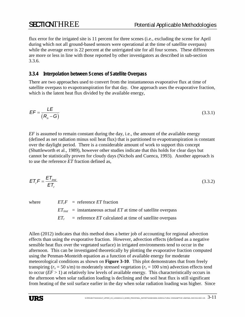
SECTIONTHREE Potential Applicable Methodologies
N:\PROJECTS\22243147_UPPER_CO_LOSSES\12.0_WORD_PROC\FINAL_REPORT\ASSESSING AGRICULTURAL CONSUMPTIVE USEFINAL.DOCX\31-DEC-13\\ 3-11
flux error for the irrigated site is 11 percent for three scenes (i.e., excluding the scene for April during which not all ground-based sensors were operational at the time of satellite overpass) while the average error is 22 percent at the unirrigated site for all four scenes. These differences are more or less in line with those reported by other investigators as described in sub-section 3.3.6.
3.3.4 Interpolation between Scenes of Satellite Overpass There are two approaches used to convert from the instantaneous evaporative flux at time of satellite overpass to evapotranspiration for that day. One approach uses the evaporative fraction, which is the latent heat flux divided by the available energy,
( )=
−n
LEEFR G
(3.3.1)
EF is assumed to remain constant during the day, i.e., the amount of the available energy (defined as net radiation minus soil heat flux) that is partitioned to evapotranspiration is constant over the daylight period. There is a considerable amount of work to support this concept (Shuttleworth et al., 1989), however other studies indicate that this holds for clear days but cannot be statistically proven for cloudy days (Nichols and Cuenca, 1993). Another approach is to use the reference ET fraction defined as,
= instr
r
ETET FET
(3.3.2)
where ETrF = reference ET fraction
ETinst = instantaneous actual ET at time of satellite overpass
ETr = reference ET calculated at time of satellite overpass
Allen (2012) indicates that this method does a better job of accounting for regional advection effects than using the evaporative fraction. However, advection effects (defined as a negative sensible heat flux over the vegetated surface) in irrigated environments tend to occur in the afternoon. This can be investigated theoretically by plotting the evaporative fraction computed using the Penman-Monteith equation as a function of available energy for moderate meteorological conditions as shown on Figure 3-10. This plot demonstrates that from freely transpiring (rs = 50 s/m) to moderately stressed vegetation (rs = 100 s/m) advection effects tend to occur (EF > 1) at relatively low levels of available energy. This characteristically occurs in the afternoon when solar radiation loading is declining and the soil heat flux is still significant from heating of the soil surface earlier in the day when solar radiation loading was higher. Since
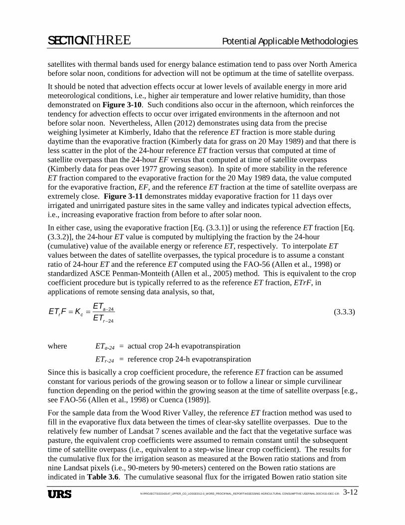
SECTIONTHREE Potential Applicable Methodologies
N:\PROJECTS\22243147_UPPER_CO_LOSSES\12.0_WORD_PROC\FINAL_REPORT\ASSESSING AGRICULTURAL CONSUMPTIVE USEFINAL.DOCX\31-DEC-13\\ 3-12
satellites with thermal bands used for energy balance estimation tend to pass over North America before solar noon, conditions for advection will not be optimum at the time of satellite overpass.
It should be noted that advection effects occur at lower levels of available energy in more arid meteorological conditions, i.e., higher air temperature and lower relative humidity, than those demonstrated on Figure 3-10. Such conditions also occur in the afternoon, which reinforces the tendency for advection effects to occur over irrigated environments in the afternoon and not before solar noon. Nevertheless, Allen (2012) demonstrates using data from the precise weighing lysimeter at Kimberly, Idaho that the reference ET fraction is more stable during daytime than the evaporative fraction (Kimberly data for grass on 20 May 1989) and that there is less scatter in the plot of the 24-hour reference ET fraction versus that computed at time of satellite overpass than the 24-hour EF versus that computed at time of satellite overpass (Kimberly data for peas over 1977 growing season). In spite of more stability in the reference ET fraction compared to the evaporative fraction for the 20 May 1989 data, the value computed for the evaporative fraction, EF, and the reference ET fraction at the time of satellite overpass are extremely close. Figure 3-11 demonstrates midday evaporative fraction for 11 days over irrigated and unirrigated pasture sites in the same valley and indicates typical advection effects, i.e., increasing evaporative fraction from before to after solar noon.
In either case, using the evaporative fraction [Eq. (3.3.1)] or using the reference ET fraction [Eq. (3.3.2)], the 24-hour ET value is computed by multiplying the fraction by the 24-hour (cumulative) value of the available energy or reference ET, respectively. To interpolate ET values between the dates of satellite overpasses, the typical procedure is to assume a constant ratio of 24-hour ET and the reference ET computed using the FAO-56 (Allen et al., 1998) or standardized ASCE Penman-Monteith (Allen et al., 2005) method. This is equivalent to the crop coefficient procedure but is typically referred to as the reference ET fraction, ETrF, in applications of remote sensing data analysis, so that,
24
24
ar c
r
ETET F KET
−
−
= = (3.3.3)
where ETa-24 = actual crop 24-h evapotranspiration
ETr-24 = reference crop 24-h evapotranspiration
Since this is basically a crop coefficient procedure, the reference ET fraction can be assumed constant for various periods of the growing season or to follow a linear or simple curvilinear function depending on the period within the growing season at the time of satellite overpass [e.g., see FAO-56 (Allen et al., 1998) or Cuenca (1989)].
For the sample data from the Wood River Valley, the reference ET fraction method was used to fill in the evaporative flux data between the times of clear-sky satellite overpasses. Due to the relatively few number of Landsat 7 scenes available and the fact that the vegetative surface was pasture, the equivalent crop coefficients were assumed to remain constant until the subsequent time of satellite overpass (i.e., equivalent to a step-wise linear crop coefficient). The results for the cumulative flux for the irrigation season as measured at the Bowen ratio stations and from nine Landsat pixels (i.e., 90-meters by 90-meters) centered on the Bowen ratio stations are indicated in Table 3.6. The cumulative seasonal flux for the irrigated Bowen ratio station site
SECTIONTHREE Potential Applicable Methodologies
N:\PROJECTS\22243147_UPPER_CO_LOSSES\12.0_WORD_PROC\FINAL_REPORT\ASSESSING AGRICULTURAL CONSUMPTIVE USEFINAL.DOCX\31-DEC-13\\ 3-13
was 746 millimeters compared to 763 millimeters based on Landsat data. For the unirrigated site, the results were 498 millimeters for the Bowen ratio station and 511 millimeters for the composite of nine Landsat pixels centered at the Bowen ratio site. These favorable results compare well with those reported by other investigators as described in sub-section 3.3.6.
3.3.5 Results: Spatial Distribution of Actual Evapotranspiration The analysis to compute the evaporative flux is carried out on a pixel by pixel basis over the Landsat scene of interest. The results are then distributed spatially using either a remote sensing data analysis platform (e.g., ERDAS IMAGINE) or a geographic information system platform (e.g., ArcGIS), or combination of the two. The results for the four cloud-free days of Landsat 7 data over the Wood River Valley in 2004 are demonstrated on Figures 3-12 (a) and (b). The lands that came under the KBRT irrigation forbearance program are designated in the figures. It can be observed that the unirrigated lands tend to have a considerably reduced latent heat flux as the growing season progresses and these lands have declining soil moisture contents. Integrating the evaporative flux values over the growing season as described above, Cuenca et al. (2013) was able to show a decrease in evaporative flux of 173 millimeters on KBRT lands compared to the irrigated lands over the entire growing season (see Table 3.6) Given the dimensions of the unirrigated fields, the Landsat platform was perfectly suited to the task of differentiating irrigated and unirrigated crop response over the Wood River Valley.
3.3.6 Sample Results from Other Investigations The results described above for the Wood River Valley are given only as an example of the procedure and applicability of remote sensing data, specifically Landsat data, to evaluation of actual crop water use and irrigation effects. While these results are felt to be representative, there are numerous other results in the literature, in training manuals, or other sources that can be reported. Just as a review, the results reported for the Wood River Valley study indicated an average difference between estimated and measured instantaneous LE fluxes on the order of 10 percent for an irrigated site and on the order of 20 percent for the unirrigated site. The seasonal cumulative differences between the Bowen ratio stations and the combination of nine Landsat pixels (i.e., 90-meters by 90-meters) centered on the Bowen ratio station were surprisingly close. Assuming that the Bowen ratio stations represent “ground truth,” the differences were 17 millimeters out of 746 millimeters for the irrigated site and 13 millimeters out of 498 millimeters for the unirrigated site.
As indicated previously, there are assumptions and errors in all ground-based evaporative flux measurements except for those acquired with a precise weighing lysimeter, which are typically very precise, e.g., able to measure evaporative flux on the order of 0.03 to 0.15 millimeter equivalent depth of water, and very accurate. The only time when lysimeters are not representative is when crop or soil management practices on the lysimeter differ from those of field conditions, or when the lysimeter is not surrounded by the same vegetation as within the lysimeter, in which case there is the potential for edge effects.
Results of comparison of instantaneous flux measurements are indicated in Table 3.7. This table compares USDA lysimeter measured fluxes (Kimberly, ID) with that of Landsat overpasses for various crops over different years using the METRIC system of data analysis. While there is a rather larger range of differences, from 0 to 45 percent assuming the lysimeter is ground truth
SECTIONTHREE Potential Applicable Methodologies
N:\PROJECTS\22243147_UPPER_CO_LOSSES\12.0_WORD_PROC\FINAL_REPORT\ASSESSING AGRICULTURAL CONSUMPTIVE USEFINAL.DOCX\31-DEC-13\\ 3-14
(excluding the difference for 18 April 1989, which has a very small value of lysimeter-measured flux and therefore a large percent error), the mean absolute value of the differences is 14.7 percent. As part of the METRIC training material, Allen (2012) indicates seasonal total estimated crop ET using Landsat data compared to the precise weighing lysimeter at the USDA station, Kimberly, ID for sugar beets (1989) and for a drainage lysimeter at Montpellier, ID for forage grass. For sugar beets at Kimberly, the seasonal lysimeter-measured ET is 718 millimeters while that estimated using Landsat data with METRIC is 714 millimeters. For the forage grass at Montpellier, the lysimeter-measured ET is 388 millimeters and that estimated using Landsat with the surface energy balance algorithm for land (SEBAL) approach is 405 millimeters.
Irmak et al. (2011) compared Bowen ratio measurements over corn at Clay Center, NB with Landsat 5 images analyzed using METRIC for 2005 (4 images) and 2006 (4 images). All components of the radiation balance and energy balance were reported. Assuming the Bowen ratio data were ground truth, the average error for net radiation was 2 to 5 percent, soil heat flux 15 to 22 percent, sensible het flux 38 to 16 percent, and latent heat flux 8 to 13 percent, all values given for 2005 and 2006, respectively. As in the example for the Wood River Valley, the agreement for the net radiation data is impressive and the error in the latent heat flux results are in a similar range as in the case of the irrigated site (KL04).
Morton et al. (2013) demonstrated a range of differences in ground-based versus Landsat estimated ET for five Bowen ratio sites (multiple years) and four eddy covariance sites (multiple years) in Nevada for a total of 16 estimates of seasonal crop ET. [Morton et al. (2013) indicated that the Bowen ratio and eddy covariance daily ET measurements were assumed by Maurer et al. (2006) to be accurate to within 12 percent of actual ET based on the literature and direct comparison at one site.] The Landsat scenes for this study were evaluated using an automated METRIC calibration scheme. The absolute value of the error in seasonal ET, assuming the ground-based stations are ground-truth, ranges from 1 to 27 percent with a mean value of 11 percent.
In related work, Beamer et al. (2013 and personal communication) experienced difficulties resolving the latent heat flux using METRIC in very arid sites in Nevada, with higher values of H and G and lower values of LE. The uncertainty in the relatively high values of H and G determined using METRIC for these arid sites obscured the signal for the relatively small values of LE. This difficulty is also probably related to the limited range of surface temperatures in very arid sites between the “hot” and “cold” pixels needed for the iterative scheme to compute the sensible heat flux. In addition, stratified rangeland soils produce lower G than predicted by the algorithm designed for agricultural soils used in METRIC, and sensible heat calculations can overestimate H over sparsely vegetated shrubland (from the METRIC manual). Beamer et al. (2013) therefore computed an Enhanced Vegetation Index (EVI) (Nagler et al., 2005) using Landsat data to compute the latent heat flux using regression analysis between the EVI and measured ET values from Bowen ratio and eddy covariance stations.
Kalma et al. (2008), in comparing some 30 validations of various remote sensing methods applied to evaporative flux measurements, indicated difference on the order of 15 to 30 percent. Kalma et al. (2008) did not evaluate the potential error in the ground-based measurements, but indicated a possible error in the range of 10 to 15 percent. Wilson et al. (2002) indicated a mean energy balance closure error on the order of 20 percent for 22 FLUXNET sites over 50 site-years
SECTIONTHREE Potential Applicable Methodologies
N:\PROJECTS\22243147_UPPER_CO_LOSSES\12.0_WORD_PROC\FINAL_REPORT\ASSESSING AGRICULTURAL CONSUMPTIVE USEFINAL.DOCX\31-DEC-13\\ 3-15
using eddy covariance instrumentation. A systematic underestimation of the latent and sensible heat fluxes was the source of the closure errors reported by Wilson et al. (2002).
3.3.7 Comparison of Meteorological-based Methods with Remote Sensing-based Methods An example comparison of meteorological-based methods with remote sensing-based methods is indicated in Table 3.8 for illustrative purposes. The assumed meteorological-based method is the ASCE standardized Penman-Monteith. The assumed remote sensing method is one that incorporates moderate resolution thermal band data from Landsat 7 and Landsat 8, e.g., METRIC method. These methods are compared for illustrative purposes only, but do indicate the major attributes in terms of pros and cons of both approaches. This table can be used as the basis of discussion to contrast advantages and disadvantages of the respective methods in the Upper Colorado River Basin.
ALTERNATIVE DATA PROCESSING PROCEDURES 3.4In this sub-section, some alternatives are presented in comparison to the standard METRIC-based approach discussed in the previous sub-section.
3.4.1 RESET The RESET procedure was used by David Eckhardt, Bureau of Reclamation, for estimation of actual crop water use following the procedure of Luis Garcia and Aymn Elhaddad of CSU. This procedure was successfully used on a trial basis but is not an operational Reclamationprogram. It has been applied by Eckhardt to two study areas: one in the Sacramento Valley of California for the 2008 and 2009 growing seasons, and one in western Colorado for the 2006 growing season. Eckhardt automated the sensible heat flux model and substituted some of the METRIC algorithms where it made sense. He also modified some data inputs, like using MODIS precipitable water vapor images to calculate band-specific atmospheric transmittance values, using NLDAS-2 wind speed data for the sensible heat flux model, and using NLDAS-2 DSRF (downward shortwave radiation flux), specific humidity, and atmospheric pressure data to improve 24-hour net radiation estimates. It should be noted that one objective was to minimize need for local meteorological data. Refer to Eckhardt (2013) for a full description of this method.
3.4.2 ArcGIS using Python and other Procedures Morton et al. (2013) describe an automated procedure using a statistical approach based on ETrF distributions to do automatic rather than manual calibration of the sensible heat flux parameter of the METRIC model for ET. While this method looks promising and compares fairly well with manual calibration of experienced users, the method is at this point experimental and has only been tested on a few sites in Nevada. It should be noted that the objective of this work was to avoid the time consuming manual selection of hot and cold pixels to bracket the sensible heat calculation for a Landsat scene. Whether such a procedure reduces the bias in the computed ET
SECTIONTHREE Potential Applicable Methodologies
N:\PROJECTS\22243147_UPPER_CO_LOSSES\12.0_WORD_PROC\FINAL_REPORT\ASSESSING AGRICULTURAL CONSUMPTIVE USEFINAL.DOCX\31-DEC-13\\ 3-16
as recently described by Long and Singh (2013) is not clear. Refer to Morton et al. (2013) for a full description of the procedure.
3.4.3 TOPS-SIMS This is an automated procedure of Forrest Melton (NASA Ames) using Landsat data and the NASA Earth Exchange (NEX) supercomputer system to determine spatial distribution of crop coefficients based on NDVI (ignoring soil evaporation). This procedure requires a ground-based micrometeorological network to compute reference ET and mapping of crop distribution by field. The spatially distributed crop coefficients are then multiplied by the reference ET to get the maximum expected crop ET. This procedure does not compute actual crop ET. Refer to Melton et al. (2012) for a full description of the procedure.
3.4.4 Automated METRIC Procedure Similar to the work done by Morton et al. (2013), Allen et al. (2013) have attempted to automate the CIMEC procedure, specifically the selection of the hot and cold pixels for the Landsat scene, within the framework of METIC analysis using an ERDAS IMAGINE platform. The initial calibration pixels are based on NDVI and surface temperature thresholds using an automated procedure. The calibration procedure isolates a subpopulation of candidate end-member pixels from which the user selects the pixels to apply. Color coding directs the user toward preferred pixels in the ERDAS IMAGINE application. In typical applications, Allen et al. (2013) the automated procedure limits the search to 1 percent of the area in a scene for the cold pixel and 2 percent of the area for a hot pixel. Whether such a procedure reduces the bias in the computed ET as recently described by Long and Singh (2013) is not clear. Refer to Allen et al. (2013) for a full description of the procedure.
OPERATIONAL CHALLENGES AND POTENTIAL SOLUTIONS 3.5In practice, there are a number of possible operational challenges in estimating actual consumptive use over large spatial scales and throughout the extent of each irrigation season. This sub-section discusses some of the most common challenges and potential solutions.
3.5.1 Number and Frequency of Growing Season Clear-sky Satellite Overpasses Detection of surface temperatures from satellites requires clear skies or nearly clear skies at the time of image acquisition. (If the sky is not clear, the thermal band simply returns the top of cloud temperature.) The only way to obtain more clear-sky imagery is to fly more satellites with thermal bands that are not in basically the same orbit, e.g., as is the case with Landsat 7 and the ASTER platform on the Terra satellite. Fortunately, with both Landsat 7 and Landsat 8 operational, there is the potential to double the frequency of satellite overpasses on the same location on Earth. Allen (2012) (based on analysis of Morton and Huntington, Desert Research Institute (DRI)) indicated that if the frequency of Landsat satellite overpasses were increased by a factor of two, there would be an exponential increase in the number of clear-sky images to process in many locations in the U.S.
SECTIONTHREE Potential Applicable Methodologies
N:\PROJECTS\22243147_UPPER_CO_LOSSES\12.0_WORD_PROC\FINAL_REPORT\ASSESSING AGRICULTURAL CONSUMPTIVE USEFINAL.DOCX\31-DEC-13\\ 3-17
3.5.2 Masking Cloud Affected Portions of Scenes Areas with cloud cover cannot be used for evaluation of the energy balance because even a thin cloud layer has a much lower surface temperature than the ground surface. In scenes with partial cloud cover, those areas on the ground that have been recently shaded by clouds will not reach a surface temperature representative of clear-sky conditions until sometime after the clouds have passed over. The METRIC group at the University of Idaho has developed a procedure to fill in cloud-masked areas of Landsat scenes before computing the distributed reference ET fraction, ETrF, for the scene. The ETrF data for the previous cloud-free scene and subsequent cloud-free scene are used to interpolate the expected value of ETrF for each cloud-masked pixel of the current scene. This procedure is described in detail in Appendix 19 of the METRIC manual (Allen et al., 2010).
3.5.3 Accounting for Sloping Ground in Radiation Calculations In the general case of sloping terrain, a digital elevation model (DEM) is required to determine the slope and aspect of inclined surfaces to correctly estimate solar radiation loading as a function of latitude, day of year and time of day. Processing the DEM for this purpose on a pixel by pixel basis can be done using the data processing tools built into ERDAS IMAGINE, which is typically used to process Landsat data. It can also be accomplished using ArcGIS Spatial Analyst, a MatLab Solar Radiation routine, or various other platforms for processing geospatial data.
3.5.4 Effects of Higher Elevation on Actual Evapotranspiration Application of the atmospheric lapse rate is required to account for the effects of elevation on both the radiation and energy balance. This is accounted for in the standard implementation of the METRIC procedure by use of a DEM of the Landsat scene. The “cold” pixel surface temperature is adjusted as a function of elevation and the atmospheric lapse rate (Eckhardt, 2013). The standard atmospheric lapse rate of the International Civil Aviation Organization (ICAO) is 0.0065˚C/m. Eckhardt (2013) indicated potential problems using the standard ICAO lapse rate and recommended developing unique lapse rates for each Landsat image using the surface temperatures of small lakes or reservoirs to define the relationship. Allen and Snyder (2011) indicate use of a “flat” lapse rate of 0.0065˚C/m for elevations less than 1,750 meters and a “mountain” lapse rate of 0.010˚C/m for elevations above 1,750 meters as part of routine processing of Landsat data using METRIC. This of course requires an additional data processing step, which must be set up as either a rule-based decision or requiring input of a human data analyst.
3.5.5 Availability of Ground-based Meteorological Data Data processing of thermal band remote sensing data for application of radiation and energy balances has typically used as little ground-based meteorological data as possible. However, wind speeds on the ground and for some applications even atmospheric profile data on the morning of the Landsat overpass are required to initiate the iterative process to calculate the sensible heat flux. Between the times of satellite overpasses, the actual ET of the vegetated surface is assumed to be related to the reference ET for any particular location by a constant,
SECTIONTHREE Potential Applicable Methodologies
N:\PROJECTS\22243147_UPPER_CO_LOSSES\12.0_WORD_PROC\FINAL_REPORT\ASSESSING AGRICULTURAL CONSUMPTIVE USEFINAL.DOCX\31-DEC-13\\ 3-18
linear or curvilinear reference ET fraction, ETrF. For this estimate to be robust, there must be high quality meteorological data for the area of interest on at least a daily basis. (In fact, accurate estimation of the ETrF related to the time of satellite overpass requires calculation of reference ET on an hourly basis.) A sophisticated network of recording meteorological stations is required to move to the level of ET analysis by application of remote sensing data. Numerous examples of such networks exist, e.g., AgriMet in the Pacific Northwest, CIMIS in California, the Oklahoma Mesonet network, the Nebraska High Plains Regional Climate Center Automated Weather Data Network (AWDN), the Colorado Agricultural Meteorological Network (CoAgMet), and many others. Standards for data quality control, network management and data distribution should be developed relative to the experience from the existing networks. There are also many other networks not typically used for agriculture that may be incorporated into the distribution of stations, e.g., the USGS Remote Automatic Weather Stations (RAWS) network, Union Pacific Railroad Weather Station Network in the central and western U.S., and others. But it is essential that standardized data quality control, data distribution, and data archiving protocols be developed based on consensus of the states involved for such a network to be operational and provide useful data.
3.5.6 Crop-cutting Between Dates of Satellite Overpasses The effect of crop-cutting over large spatial areas, similar to the effects of irrigation or precipitation indicated in sub-section 3.5.7, cannot be predicted and is probably in general too subtle to be recognized in a remote sensing scene, i.e., there will be a shift in the reference ET fraction, ETrF, between remote sensing scenes but the amount of that shift due to cutting is not possible to predict and therefore developing a rule-based adjustment scheme is difficult. Allen et al. (2007) and Allen and Snyder (2011) indicate the use of a cubic spline function to fit the ETrF between satellite image dates and discuss the advantages over a linear function between dates. In fact, changes in ETrF due to crop cutting would be abrupt and better modeled using a linear function. However, since the date of the cutting is generally unknown and the probability that the cutting falls between two satellite overpasses is infinitely high, a smooth function through the ETrF is a suitable compromise. The use of daily thermal band data from other satellite platforms such as MODIS is not practicable due to the spatial scale of MODIS thermal data, which are at best (i.e., after “sharpening”) 240 meters at nadir. This resolution degrades for off-nadir portions of the images.
3.5.7 Precipitation (or Irrigation) Just Before or Just After Satellite Overpass Kjaersgaard et al. (2011) discuss the fact that Landsat (or other thermal band platform) scenes will not be representative if there is precipitation just before or just after the time of satellite overpass. They indicate that the bias in the seasonal ET estimate due to surface wetting may be high or low depending on the date of satellite overpass relative to the date of wetting. Allen et al. (2007) indicate that the randomness of irrigation relative to the fixed frequency of a satellite overpass would in general tend to minimize the bias in the ET estimate. This would be true if there were enough satellite scenes to capture the variability in time of the surface conditions. However, due to the problem with cloud-free days indicated above, a seasonal ET estimate may be based on only a handful of scenes and the fewer the number of scenes the higher the potential of a bias.
SECTIONTHREE Potential Applicable Methodologies
N:\PROJECTS\22243147_UPPER_CO_LOSSES\12.0_WORD_PROC\FINAL_REPORT\ASSESSING AGRICULTURAL CONSUMPTIVE USEFINAL.DOCX\31-DEC-13\\ 3-19
Kjaersgaard et al. (2011) discuss the fusing of data from satellites with higher frequency, but reduced spatial resolution, such as MODIS, with Landsat data. They argue that the field to field variation, particularly in irrigated fields, is lost due to the fact that the 30-meter ET is based on a vegetation index that may not see the impact (due to variation in soil moisture content) that would be apparent from an energy balance analysis.
Kjaersgaard et al. (2011) demonstrate a period of precipitation preceding a Landsat 5 overpass for the southwestern portion of the Nebraska Panhandle and argue that there is a “background” evapotranspiration from bare soil that should be adjusted for so as to not bias the Landsat scene on the high side. They do this by estimating the evaporation from bare soil using a daily hydrological process model and applying it to the bare soil fraction in the scene. The model can be as simple as the FAO-56 Penman-Monteith model (Allen, 1998) using a bare soil crop coefficient to something as complex as the DAISY simulation model (Abrahamsen and Hansen, 2000). This approach requires soil texture and soil property inputs from something like the Natural Resources Conservation Service (NRCS)Soil Survey Geography( SSURGO) soil data base. Also, local meteorological data (i.e., distributed to cover the Landsat scene) for precipitation and computing something like the Penman-Monteith reference ET is required. The bare soil fraction is determined using the NDVI distribution.
The underlying assumption of using Landsat data to capture regional ET over a growing season is that remote sensing data collected on a regular interval will be used to capture the response of land surface ET that is randomized (in both time and space) due to irregular irrigation and/or precipitation. If enough cloud-free Landsat scenes are available, they should be adequate for capturing the random response of the surface during the growing season. Any hydrologic process simulation model will have some uncertainty associated with the input parameters, fitting parameters, and the fact that the model is only representative of the real system. Kjaersgaard et al. (2011) show a fair amount of adjustment in the reference ET fraction, ETrF, during certain periods of the growing season for the Nebraska sites. The estimated spatially distributed ET for a given Landsat scene is also shown to have a significant adjustment when this hydrologic modeling procedure is applied. The magnitude of this adjustment relative to the magnitude of the uncertainty in the hydrologic model over the growing season is a subject which requires further research. The Kjaersgaard et al. (2011) results are a promising proof of concept, but further research is required to evaluate this approach within an operational framework.
3.5.8 Application of Cold Irrigation Water to Crops Eckhardt (2013) explains that application of cold irrigation water due to snowmelt from streams or reservoirs can lead to errors in the estimation of the sensible and therefore latent heat fluxes using an energy balance approach. The tendency is for the calculated H to be negative (i.e., advection effects), which therefore creates values for LE that are over-predicted. Eckhardt (2012) recommends limiting the values of LE for a scene based on the distribution of NDVI. Values of LE that are over-predicted should show up as outliers on a distribution of LE to NDVI. Of course, this requires an additional data processing step and either a rule-based decision or evaluation by a human data analyst.
SECTIONTHREE Potential Applicable Methodologies
N:\PROJECTS\22243147_UPPER_CO_LOSSES\12.0_WORD_PROC\FINAL_REPORT\ASSESSING AGRICULTURAL CONSUMPTIVE USEFINAL.DOCX\31-DEC-13\\ 3-20
3.5.9 Data Input and Processing Requirements There are numerous articles describing the type of input data required to process satellite thermal band data to compute the radiation and energy balances. Using Eckhardt (2013) as an example, Landsat 7 Enhanced Thematic Mapper Plus (ETM+) and presumed to be available soon LDCM (Landsat 8) Operational Land Imager and Thermal Infrared Sensor data are the first requirement. A DEM resolved to a 30-meter grid for determination of slope and aspect required for radiation calculations is also required. Astronomical data for solar declination, hour angle, Earth-to-Sun distance and top of atmosphere direct normal solar irradiance (available from the University of Oregon Solar Radiation Monitoring Laboratory) are needed. Finally meteorological data, including solar radiation, air temperature and relative humidity, wind speed and precipitation, for the area of interest are needed on something like an hourly time step for the most flexible program of data analysis.
Data processing platforms that are specifically designed for analysis of spatially distributed remote sensing data are required. Probably the most commonly applied platform to date has been the ERDSAS IMAGINE system coupled with the ERDAS Modelmaker. Recent applications have also included using the ArcGIS platform and often output from ERDAS IMAGINE can be conveniently analyzed using ArcGIS. There are also pre-coded ERDAS extensions for ArcGIS. No doubt other platforms could also be used for remote sensing data processing, but ERDAS IMAGINE and ArcGIS have been the most commonly used platforms to date.
OUT OF THE BOX – A DIFFERENT APPROACH 3.6Recent work (Long and Singh, 2013) has indicated increased levels of uncertainty in analysis of Landsat data using SEBAL or METRIC type approaches due to the difficulty in identifying the “hot” and “cold” pixels in a scene, as well as determining the representative values of latent and sensible heat fluxes to associate with these end-member pixels. Obviously looking for automated means of determining the scene end members has been an emphasis in recent evaluation of Landsat data. This difficulty has led to an investigation of alternative methods of Landsat data analysis that do not rely on end-member pixels within the scene. An alternative approach is the type indicated by Kalma et al. (2008) as methods that use the time rate of change in surface temperature with atmospheric boundary layer) models. The ALEXI-DisALEXI approach described below is one such approach that has been applied in a number of studies. An additional persistent problem in analysis of Landsat data has been to fill the gaps between the days of clear-sky satellite overpasses. Somewhat novel approaches to address this issue have been developed to try to take advantage of the time resolution of MODIS thermal band data and the spatial resolution of Landsat data. These three topics are described in this section. It should be noted that there are ongoing discussions with the Hydrology and Remote Sensing Laboratory of the United States Department of Agriculture (USDA) to investigate practical applications of the methods covered in this sub-section.
3.6.1 Uncertainty in Analysis of Landsat Scenes While development of automated techniques for determination of the hot and cold pixels continues, there is renewed discussion of the uncertainty in the actual ET product using Landsat
SECTIONTHREE Potential Applicable Methodologies
N:\PROJECTS\22243147_UPPER_CO_LOSSES\12.0_WORD_PROC\FINAL_REPORT\ASSESSING AGRICULTURAL CONSUMPTIVE USEFINAL.DOCX\31-DEC-13\\ 3-21
data. Long and Singh (2013) discuss the impact of end-member selection on the spatial variability of actual evapotranspiration using three models including SEBAL and METRIC. They demonstrate variation in the results of spatially distributed evapotranspiration based on three cases for the cold pixel and three cases for the hot pixel, i.e., nine cases in total, which were selected by experienced evaluators of Landsat data. Long and Singh (2013) indicate that the degree of bias in the results compared to ground-based measurements from the (Soil Moisture–Atmosphere Coupling Experiment) SMACEX field campaign (Kustas et al., 2005) varied as a function of end-member selection. The choice of the end members therefore scaled the evapotranspiration rate over the entire scene. Varying the end members did not significantly modify the frequency distribution of the evaporative fraction over the scene using SEBAL or METRIC, nor the standard deviation and skew of the distribution. This is because varying the end members of the scene does not alter the model physics. But the fact that the magnitude of evapotranspiration for the entire scene is scaled up or down based on the end-member selection means that there is a significant level of uncertainty in model results. This uncertainty can be reduced, i.e., model results can be appropriately scaled, if there are ground-based measurements of evaporative flux using precise lysimeters, eddy covariance, or Bowen ratio systems within the same scene and consistent rule sets are used by analysts for pixel selection. A ground-based network necessarily incurs additional costs and requires experienced personnel to operate these systems. However, it is not clear what other means are available to reduce the uncertainty in the current evaluation of Landsat data for evapotranspiration if end member “hot” and “cold” pixels are required.
It is worth noting that Timmermans et al. (2007) indicated that adjusting Tmax or Tmin for a specific land cover, i.e., by modifying the end-member selection, could be used to calibrate the energy balance model with respect to ground-based measurements thereby reducing errors in the sensible heat flux for a specific vegetative cover. Such an action would, however, have the potential of increasing the error in the sensible heat flux for other vegetative covers within the same Landsat scene. For this reason, Long and Singh (2013) feel that current procedures for the selection of end members are less than satisfactory, somewhat subjective, not deterministic and lead to results that are less than robust in that if alternative end members were selected by another person analyzing the same scene, the magnitude of the evaporative fraction over the scene would be different. It is clear that additional effort is required with respect to selection of the hot and cold pixels in a scene to reduce the uncertainty in interpretation of Landsat results.
There is an additional consideration of uncertainty that was evident in analysis of data from the Wood RiverValley, Oregon as reported by Cuenca et al. (2013). SEBAL and METRIC have related but different ways of computing the atmospheric fluxes of the end-member hot and cold pixels. SEBAL assumes that the evapotranspiration of the hot pixel is zero and the sensible heat flux is computed as the residual of net radiation minus the soil heat flux. For the cold pixel, SEBAL assumes that the sensible heat flux is zero and that the latent heat flux for this pixel is the residual of net radiation minus the soil heat flux. METRIC typically assumes that the latent heat flux of the cold pixel is equal to the Penman-Monteith reference ET and the sensible heat flux is computed as a residual of the energy balance equation [Eq. (3.2.5)]. Like SEBAL, METRIC typically assumes that the latent heat flux of the hot pixel equals zero. However, if there is some reason to assume it is not zero, e.g., high soil moisture content in a bare soil pixel, then METRIC allows that the latent heat flux can be approximated as some fraction of the reference ET. In the study of Cuenca et al. (2013) in the Wood River Valley, high soil moisture
SECTIONTHREE Potential Applicable Methodologies
N:\PROJECTS\22243147_UPPER_CO_LOSSES\12.0_WORD_PROC\FINAL_REPORT\ASSESSING AGRICULTURAL CONSUMPTIVE USEFINAL.DOCX\31-DEC-13\\ 3-22
conditions, especially early in the growing season, necessitated that the latent heat flux for the hot pixel be set to 0.25 times the reference ET for the time of satellite overpass to represent bare soil evaporation. This step significantly improved the remote sensing results compared to those measured by the Bowen ratio stations, particularly early in the growing season.
But the fact is that setting the hot pixel latent heat flux to 0.25 times reference ET was an arbitrary value, although based on expected soil evaporation from field experience. But this value of 0.25 was estimated and not measured. In fact, the values of zero latent heat flux for the hot pixel in SEBAL and reference ET latent heat flux for the cold pixel using METRIC are also arbitrary values not based on actual measurements of hot and cold pixel ET at the time of satellite overpass. Much as scaling the Tmin and Tmax indicated by Timmermans et al., (2007) will shift the resulting spatially distributed ET for the entire scene, making the results more accurate for some vegetation covers and less accurate for other vegetation covers, the selection of the typical end points for SEBAL and METRIC will have the same effect. Again, only ground-based measurements of actual latent heat fluxes can help resolve this bias and reduce the uncertainty in analysis of Landsat data for evapotranspiration.
3.6.2 ALEXI and DisALEXI Approach This modeling approach disaggregates regional scale (103 meter) atmospheric parameters and fluxes to local (or micrometeorological) scales (101 to 102 meter) where the results can be compared to ground-based measurements or used operationally in water resources management. The Atmosphere-Land Exchange Inverse (ALEXI) regional scale model uses thermal imagery from the Geostationary Operational Environmental Satellite (GOES) at a 5-kilometer resolution along with a two-source atmospheric boundary layer model to determine air temperature at a “mixing height” of 50 meters above ground level (AGL). The disaggregated micrometeorological scale model, DisALEXI, uses thermal band data from Landsat at 60-meter resolution, which can be sharpened to 30-meter resolution using the Landsat visible and near-infrared bands (30-meter resolution) using the DisTrad algorithm. The DisALEXI model uses the 50-meter mixing height air temperature value from the two-source model and disaggregates the fluxes using the 30-meter surface radiometric temperature and fractional vegetation cover from Landsat (see Figure 3-13). The 30-meter disaggregated flux fields were re-aggregated over an area equivalent to a flux tower footprint to evaluate errors of the remote sensing derived ET in an experiment in Oklahoma. An advantage of this procedure is that GOES thermal band data are available on a 15-min time resolution and so in fact daily ET fluxes could be derived by making some assumptions. Other advantages are that the method does not require micrometeorological data over the area of interest, nor “hot” and “cold” pixels within the same scene to bracket the values of the sensible heat flux. A disadvantage is that atmospheric profile data (Tair, RHair, wind speed) from regional morning radiosonde profiles are required. An additional disadvantage is that the procedure requires the two-source (soil and plant canopy components) atmospheric boundary layer simulation model, which brings an additional level of uncertainty into the results. Most of the following discussion is taken from Anderson et al. (2004) with other references as noted.
SECTIONTHREE Potential Applicable Methodologies
N:\PROJECTS\22243147_UPPER_CO_LOSSES\12.0_WORD_PROC\FINAL_REPORT\ASSESSING AGRICULTURAL CONSUMPTIVE USEFINAL.DOCX\31-DEC-13\\ 3-23
3.6.2.1 Approach
The nested-scale downscaling approach was introduced by Norman et al. (2003) to disaggregate 5-kilometer flux estimates from a two-source ABL model to the scale of eddy covariance towers during the 1997 Southern Great Plains field experiment (SGP97). (See Figure 3-13 for examples from this experiment.) Footprint-weighted latent heat flux estimates agreed with eddy covariance tower measurements to within 12 percent (Norman et al., 2003). At the same time, Kustas et al. (2003) developed the DisTrad algorithm using the physical relationship between surface temperature and vegetation cover to “sharpen” the thermal band data using the higher resolution visible and near-infrared band data. (This procedure is described in sub-section 3.8.1.)
At the core of this approach is the two-source land surface representation coupling soil, plants and the atmosphere. The two-source model (TSM) partitions the directional radiometric temperature, Trad (φ), into soil and canopy contributions (Ts and Tc) as a function of the fractional vegetation cover at the thermal view angle φ [f (φ)] as given by,
( ) ( ) ( )4 4 41rad can soilT f T f Tϕ ϕ ϕ = + − (3.6.1)
The above equation is solved for a system of surface energy balance equations, which includes soil and canopy effects, given as,
nR H LE G= + + (3.6.2)
n soil soil soilR H LE G− = + + (3.6.3)
n can can canR H LE− = + (3.6.4)
where Rn = net radiation
H = sensible heat flux
LE = latent heat flux
and where the soil and can subscripts refer to soil and vegetative canopy components, respectively. Lower boundary conditions are specified by the remote sensing data from both thermal and visible bands. Upper boundary conditions for air temperature and wind speed, used along with vegetation cover and surface roughness to compute transport resistances, need to be specified to compute Hsoil and Hcan assuming a series resistance network as shown in the left-hand side of Figure 3-14. A modified Priestley-Taylor (1972) function is used to provide for an initial estimate of canopy evapotranspiration, LEcan, and the soil latent heat flux, LEsoil, is computed as a residual. The TSM provides for the dependence of apparent surface temperature
SECTIONTHREE Potential Applicable Methodologies
N:\PROJECTS\22243147_UPPER_CO_LOSSES\12.0_WORD_PROC\FINAL_REPORT\ASSESSING AGRICULTURAL CONSUMPTIVE USEFINAL.DOCX\31-DEC-13\\ 3-24
on view angle φ as indicated in Eq. (3.6.1) and on Figure 3-14. This is important in applications of remote sensing when parts of scenes are viewed off nadir.
The TSM requires specification of temperature above the canopy and is sensitive to biases in this input. For regional scale applications, the TSM has been coupled with an atmospheric boundary layer simulation model (McNaughten and Spriggs, 1986). It should be noted that the regional scale ALEXI model requires information on the wind speed field at 50-meter AGL and ABL temperature and humidity mixing ratio profiles (5- to 8-kilometer altitude) at each 5-kilommeter grid cell to compute transport resistances and atmospheric corrections. These input fields are created using standard observations from the synoptic weather and radiosonde networks (ASOS/AWOS) (Anderson et al., 2004). Vegetation cover fraction at a 1-kilometer scale is also required and determined using NDVI computed using data from the Advanced Very High Resolution Radiometer (AVHRR) satellite. See Table 3.9 taken from Anderson et al. (2004) for input data requirements and data sources for the ALEXI and DisALEXI models.
3.6.2.2 ALEXI
ALEXI is a coupled TSM-ABL simulation model. The lower boundary conditions for ALEXI are provided by TIR observations taken at two times in the morning, i.e., shortly after sunrise and about four hours later. The geostationary GOES platform (5-kilommeter resolution) is adequate for this input. For the Oklahoma experiment reviewed in Anderson et al. (2004), thermal imager data were available every 15 minutes at an average nadir viewing angle of about 40° and a nominal spatial resolution of 5 kilometers. The ABL model relates the modeled rise in air temperature above the canopy and the resulting growth of the ABL to the time-integrated influx of sensible heat over the period of the two measurements. Use of the time-differential TIR data reduces model sensitivity to errors in absolute surface temperature due to sensor calibration and atmospheric and surface emissivity corrections. The early morning atmospheric profile of temperature is used in the ABL simulation model; air temperature and mixing ratio profiles are used in atmospheric correction of the TIR imagery using the procedure described in French et al. (2003). A vegetation-cover correction for surface emissivity was applied as given by Mecikalski et al. (1999).
Downwelling solar and longwave radiation are estimated at each ALEXI pixel using hourly 20-kilometer GOES data (Diak et al., 1996, 2000). Estimates of vegetation cover were derived using the procedure of Choudhury et al. (1994) with biweekly NDVI based on AVHRR data (Eidenshink, 1992). The vegetative cover estimates were used with the land surface classification for the US (USGS, 1995) for surface parameters of surface roughness, displacement height and radiometric properties.
3.6.2.3 DisALEXI
The DisALEXI algorithm was developed by Norman et al. (2003) and is a two-step process. Referring to Figure 3-14, ALEXI is first executed at 5-kilometer resolution to estimate the air temperature at 50-meters AGL. This air temperature is then held constant and the two-source model is executed with high resolution surface temperature and vegetation cover data, e.g., at 30-meter resolution as shown on Figure 3-16. The DisALEXI approach assumes that horizontal fluxes are small in comparison with vertical fluxes and that conditions at 50-meters AGL are constant on the 5-kilometer horizontal scale. Both of these assumptions may be violated in
SECTIONTHREE Potential Applicable Methodologies
N:\PROJECTS\22243147_UPPER_CO_LOSSES\12.0_WORD_PROC\FINAL_REPORT\ASSESSING AGRICULTURAL CONSUMPTIVE USEFINAL.DOCX\31-DEC-13\\ 3-25
strongly heterogeneous landscapes subject to advection and small-scale surface-atmosphere coupling. Some work has been done to try to adjust for such conditions in application of the DisALEXI approach (Kustas and Albertson, 2003).
3.6.2.4 Comparison to Ground-Based Measurements
Flux estimates using the ALEXI/DisALEXI scheme were compared with fluxes measured by eddy covariance stations in the Oklahoma experiment (Brotzge et al., 1999). The closure error of the eddy covariance stations [defined as the sum of the atmospheric fluxes divided by the available energy, or (H + LE)/(Rn – G)] ranged between 95 and < 40 percent (Anderson et al., 2004). Closure was forced by increasing the atmospheric fluxes, but keeping the Bowen ratio, H/LE, constant. Fluxes from one site that consistently showed a closure of < 40 percent were not used. Comparisons were made with six eddy covariance stations over a total of four exceptionally clear days with Landsat 7 overpasses during 2000-01. The high resolution DisALEXI results were reaggregated to correspond to the footprint of the flux towers for comparison with the ground data using the flux tower footprint model of Schuepp et al. (1990, 1992).
The number of instantaneous observations was 30 and the error, defined as the mean absolute difference divided by the mean observed flux, was between 9 and 10 percent (depending on the thermal sharpening and soil heat flux estimation techniques used). The number of cases for evaluating integrated daytime fluxes (assuming a constant evaporative fraction) was 28 and the mean error was 12.2 percent.
3.6.2.5 Comparison of Remote Sensing Platforms and Methods
An attempt to compare remote sensing platforms and ET estimating methods pertinent to this report is carried out in Tables 3.10 and 3.11. Table 3.10 indicates the major attributes of thermal band remote sensing platforms, including MODIS and Landsat 7 and 8, for which example applications are given in this report. Table 3.11 indicates the major attributes of the METRIC and ALEXI/DisALEXI computational schemes covered in this report. Moving forward, the best attributes of the available remote sensing platforms and computational schemes should be applied to optimize data analysis and data management for the purpose of evaluating actual crop ET in the Upper Colorado River Basin. This should be considered a dynamic rather than static decision as at the very least new algorithms will be developed to make the best use of available remote sensing data. Different remote sensing platforms will also evolve, but this will be on a much longer time scale.
3.6.3 Gap Filling Using Data Fusion A difficulty in using high spatial resolution thermal band data operationally is the gap in time between Landsat satellite overpasses. This will be somewhat alleviated when Landsat 7 and 8 fly in synchronous orbits, thereby leaving a gap of approximately eight days between overpasses. But the days between overpasses must be filled in with evapotranspiration estimates for water resources management. Recently the concept of using data fusion from geostationary and polar orbiting satellites has been proposed and tested to enable scenes of daily evapotranspiration to be produced. In the commonly applied pairing of Landsat and MODIS data (LMP), the objective is
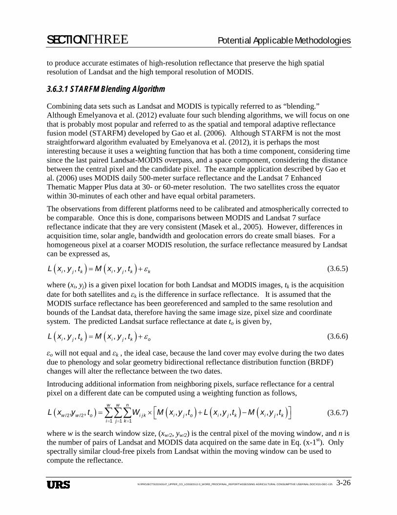
SECTIONTHREE Potential Applicable Methodologies
N:\PROJECTS\22243147_UPPER_CO_LOSSES\12.0_WORD_PROC\FINAL_REPORT\ASSESSING AGRICULTURAL CONSUMPTIVE USEFINAL.DOCX\31-DEC-13\\ 3-26
to produce accurate estimates of high-resolution reflectance that preserve the high spatial resolution of Landsat and the high temporal resolution of MODIS.
3.6.3.1 STARFM Blending Algorithm
Combining data sets such as Landsat and MODIS is typically referred to as “blending.” Although Emelyanova et al. (2012) evaluate four such blending algorithms, we will focus on one that is probably most popular and referred to as the spatial and temporal adaptive reflectance fusion model (STARFM) developed by Gao et al. (2006). Although STARFM is not the most straightforward algorithm evaluated by Emelyanova et al. (2012), it is perhaps the most interesting because it uses a weighting function that has both a time component, considering time since the last paired Landsat-MODIS overpass, and a space component, considering the distance between the central pixel and the candidate pixel. The example application described by Gao et al. (2006) uses MODIS daily 500-meter surface reflectance and the Landsat 7 Enhanced Thematic Mapper Plus data at 30- or 60-meter resolution. The two satellites cross the equator within 30-minutes of each other and have equal orbital parameters.
The observations from different platforms need to be calibrated and atmospherically corrected to be comparable. Once this is done, comparisons between MODIS and Landsat 7 surface reflectance indicate that they are very consistent (Masek et al., 2005). However, differences in acquisition time, solar angle, bandwidth and geolocation errors do create small biases. For a homogeneous pixel at a coarser MODIS resolution, the surface reflectance measured by Landsat can be expressed as,
( ) ( ), , , ,i j k i j k kL x y t M x y t ε= + (3.6.5)
where (xi, yj) is a given pixel location for both Landsat and MODIS images, tk is the acquisition date for both satellites and εk is the difference in surface reflectance. It is assumed that the MODIS surface reflectance has been georeferenced and sampled to the same resolution and bounds of the Landsat data, therefore having the same image size, pixel size and coordinate system. The predicted Landsat surface reflectance at date to is given by,
( ) ( ), , , ,i j k i j k oL x y t M x y t ε= + (3.6.6)
εo will not equal and εk , the ideal case, because the land cover may evolve during the two dates due to phenology and solar geometry bidirectional reflectance distribution function (BRDF) changes will alter the reflectance between the two dates.
Introducing additional information from neighboring pixels, surface reflectance for a central pixel on a different date can be computed using a weighting function as follows,
( ) ( ) ( ) ( )/2 /21 1 1
, , , , , , , ,w w n
w w o i j k i j o i j k i j ki j k
L x y t W M x y t L x y t M x y t= = =
= × + − ∑∑∑ (3.6.7)
where w is the search window size, (xw/2, yw/2) is the central pixel of the moving window, and n is the number of pairs of Landsat and MODIS data acquired on the same date in Eq. (x-1st). Only spectrally similar cloud-free pixels from Landsat within the moving window can be used to compute the reflectance.
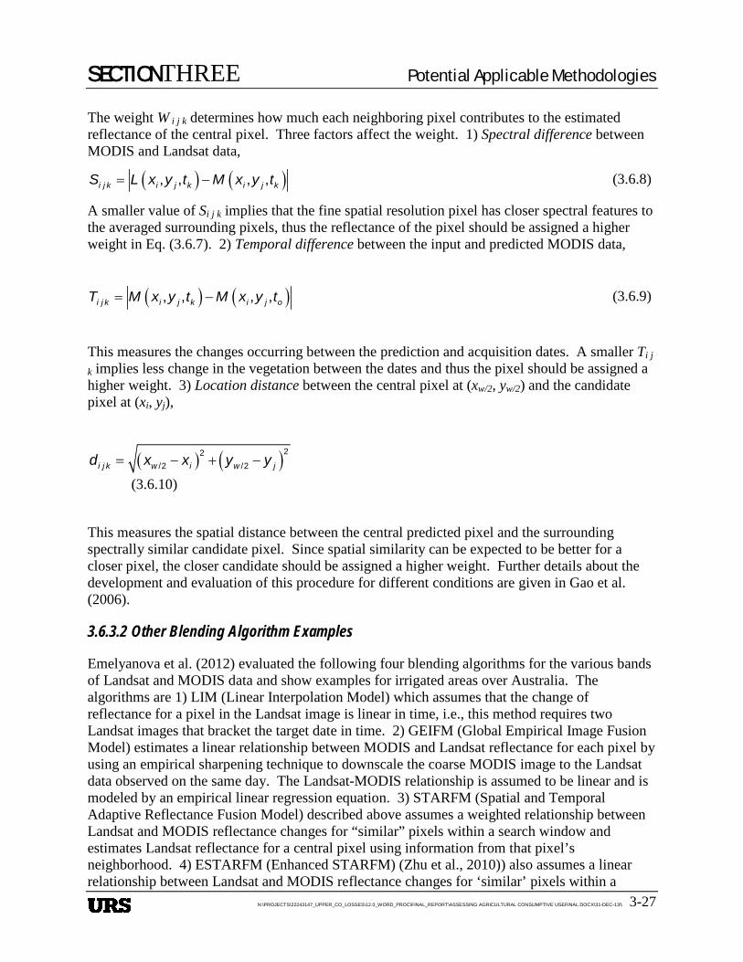
SECTIONTHREE Potential Applicable Methodologies
N:\PROJECTS\22243147_UPPER_CO_LOSSES\12.0_WORD_PROC\FINAL_REPORT\ASSESSING AGRICULTURAL CONSUMPTIVE USEFINAL.DOCX\31-DEC-13\\ 3-27
The weight W i j k determines how much each neighboring pixel contributes to the estimated reflectance of the central pixel. Three factors affect the weight. 1) Spectral difference between MODIS and Landsat data,
( ) ( ), , , ,i j k i j k i j kS L x y t M x y t= − (3.6.8)
A smaller value of Si j k implies that the fine spatial resolution pixel has closer spectral features to the averaged surrounding pixels, thus the reflectance of the pixel should be assigned a higher weight in Eq. (3.6.7). 2) Temporal difference between the input and predicted MODIS data,
( ) ( ), , , ,i j k i j k i j oT M x y t M x y t= − (3.6.9)
This measures the changes occurring between the prediction and acquisition dates. A smaller Ti j
k implies less change in the vegetation between the dates and thus the pixel should be assigned a higher weight. 3) Location distance between the central pixel at (xw/2, yw/2) and the candidate pixel at (xi, yj),
( ) ( )22/2 /2i j k w i w jd x x y y= − + −
(3.6.10)
This measures the spatial distance between the central predicted pixel and the surrounding spectrally similar candidate pixel. Since spatial similarity can be expected to be better for a closer pixel, the closer candidate should be assigned a higher weight. Further details about the development and evaluation of this procedure for different conditions are given in Gao et al. (2006).
3.6.3.2 Other Blending Algorithm Examples
Emelyanova et al. (2012) evaluated the following four blending algorithms for the various bands of Landsat and MODIS data and show examples for irrigated areas over Australia. The algorithms are 1) LIM (Linear Interpolation Model) which assumes that the change of reflectance for a pixel in the Landsat image is linear in time, i.e., this method requires two Landsat images that bracket the target date in time. 2) GEIFM (Global Empirical Image Fusion Model) estimates a linear relationship between MODIS and Landsat reflectance for each pixel by using an empirical sharpening technique to downscale the coarse MODIS image to the Landsat data observed on the same day. The Landsat-MODIS relationship is assumed to be linear and is modeled by an empirical linear regression equation. 3) STARFM (Spatial and Temporal Adaptive Reflectance Fusion Model) described above assumes a weighted relationship between Landsat and MODIS reflectance changes for “similar” pixels within a search window and estimates Landsat reflectance for a central pixel using information from that pixel’s neighborhood. 4) ESTARFM (Enhanced STARFM) (Zhu et al., 2010)) also assumes a linear relationship between Landsat and MODIS reflectance changes for ‘similar’ pixels within a
SECTIONTHREE Potential Applicable Methodologies
N:\PROJECTS\22243147_UPPER_CO_LOSSES\12.0_WORD_PROC\FINAL_REPORT\ASSESSING AGRICULTURAL CONSUMPTIVE USEFINAL.DOCX\31-DEC-13\\ 3-28
search window. However, the ESTARFM algorithm for identification of “similar” pixels is more advanced (Zhu et al., 2010) but requires two L-M pairs unlike STARFM, which can produce Landsat simulations from one L-M pair.
An example application of the various algorithms for the Lower Gwydir Catchment study site in New South Wales, Australia, is shown in Figure 3-15. Emelyanova et al. (2012) noted that the computing time to process a six-band image of the Gwydir study site made up of 3200 by 2720 pixels varied from less than a minute for the simpler LIM and GEIFM algorithms to approximately 6 hours for the more sophisticated STARFM algorithm and close to twice that long (~ 12 hours) for the ESTARFM algorithm. All runs were made on the same modern personal computer with Intel® Core™ i7-2760M processor (204 GHz, 6 MB cache) with all data stored and results written to the local hard drive. The more sophisticated algorithms were not necessarily more accurate than the simpler algorithms. Emelyanova et al. (2012) show that the root mean squared error was a function of the scene being evaluated and the particular band. For some combinations of scenes and bands, the simpler LIM and GEIFM algorithms were more accurate. Having said that, Emelyanova et al. (2012) indicate that the STARFM algorithm appears to be popular with the remote sensing community based on the number of published applications since it was developed by Gao et al. in 2006. It should be noted that the STARFM computing package is available for download from the NASA Landsat Ecosystem Disturbance Adaptive Processing System (LEDAPS) web page (http://ledaps.nascom.nasa.gov/tools/tools.html).
Finally, an application of the ALEXI-DisALEXI two-source model together with the STARFM interpolating algorithm was made by Anderson et al. (2013) for daily evapotranspiration over a nine-day period near Orlando, FL in 2002 and is shown in Figure 3-16. Because the ALEXI approach was used with GOES data, no local meteorological station data were needed, although the atmospheric profile and other data noted in sub-section 3.5.5 were required. The gap between the Landsat 5 overpass on DOY 328 and the Landsat 7 overpass on DOY 336 was filled using the STARFM algorithm with MODIS data resulting in an estimation of daily evapotranspiration. Finally a comparison of the predicted ET compared to the ET derived from Landsat 7 thermal band data indicated an average difference of 9 percent between the two methods. This is certainly an acceptable level of difference for many water resources management requirements.
REMOTE SENSING RECOMMENDATIONS 3.7
3.7.1 Definition of Remote Sensing Platform and Data Analysis Requirements The method of data analysis should be a physics-based retrieval of actual evapotranspiration from the vegetated or bare soil surface at time of satellite overpass using a combination of visible and thermal-band remote sensing data. The physics-based analysis shall first compute the four components of the radiation balance, i.e., incoming and reflected shortwave radiation, and upwelling and downwelling longwave radiation. The physics-based analysis shall next compute the four components of the energy balance, i.e., net radiation, soil heat flux, sensible heat flux and latent heat flux (i.e., evapotranspiration). Computation for the sensible heat flux shall include effects of surface roughness, aerodynamic resistance, atmospheric stability and the potential for advection. The computed latent heat flux will represent the actual
SECTIONTHREE Potential Applicable Methodologies
N:\PROJECTS\22243147_UPPER_CO_LOSSES\12.0_WORD_PROC\FINAL_REPORT\ASSESSING AGRICULTURAL CONSUMPTIVE USEFINAL.DOCX\31-DEC-13\\ 3-29
evapotranspiration of the vegetated or bare soil surface, not a maximum or indexed value. All components of the energy balance are to be computed on a pixel-by-pixel basis. The remote sensing data shall be collected at a spatial scale useful to irrigated agriculture, i.e., tens of meters, using data from a moderate level resolution remote sensing platform so that the results of the energy balance analysis make it possible to distinguish irrigated from unirrigated fields. The remote sensing data shall be collected at a temporal scale useful to decision making in irrigated agriculture, i.e., a few days or weekly. Micrometeorological data (representative of a reference environment or conditioned to represent a reference environment) on an hourly or sub-hourly time step and distributed over the irrigated area of interest will be used in support of the energy balance computations at the time of satellite overpass.
3.7.2 Application of Satellite Remote Sensing Data Numerous examples are given in this report of the application of satellite optical band and thermal band data to estimation of radiation and energy balances at a scale pertinent to irrigated agriculture. Such a program of data analysis is doable, although it has never been done on the scale required for application to the Upper Colorado River Basin. Although there is a certain amount of uncertainty and error associated with measurements made from an orbit of over 700 kilometers above the surface of the Earth, there is also considerable error made by application of the modified Blaney-Criddle method for reference ET (Jensen et al., 1990). It should also be clearly noted that application of the radiation and energy balances returns an estimate of actual evapotranspiration by the vegetated surface. Application of the modified Blaney-Criddle method does not provide an estimate of actual crop water use unless every field has a crop coefficient associated with the crop and irrigation management of that particular field. The objective of the USGS Landsat team is to make Landsat 7 and Landsat 8 data freely available in a timely manner. The availability of Landsat scenes from the EROS data center and availability of Landsat data for each band for those images from the WELD website are clear demonstrations of the potential accessibility of data acquisition. New developments to produce operational versions of ALEXI/GOES results by NOAA point to the possibility of using DisALEXI with Landsat data for field scale evaluation of consumptive water use. The potential to blend Landsat data with MODIS daily thermal band data at a pseudo Landsat spatial scale using a weighting function points to the possibility of gap filling Landsat data in time. The recommendation is to proceed with establishing a program of Landsat and other satellite data acquisition and analysis incorporating a physics-based radiation balance and energy balance approach at a “sharpened” resolution for the thermal band data.
3.7.3 Ground-based Meteorological and Evaporative Flux Networks As indicated in sub-section 3.5.5, data from a ground-based meteorological network is required for input data on the day of satellite overpass for estimation of the reference ET fraction and for estimation of reference ET for periods between satellite overpasses. Such a network can also be used to validate the ALEXIS/GOES estimates of distribution of meteorological data over CONUS in the region of the Upper Colorado River Basin. The network should collect data for computation of reference ET using the Penman-Monteith method, including at least solar radiation, air temperature and relative humidity, wind speed, and precipitation on an hourly time
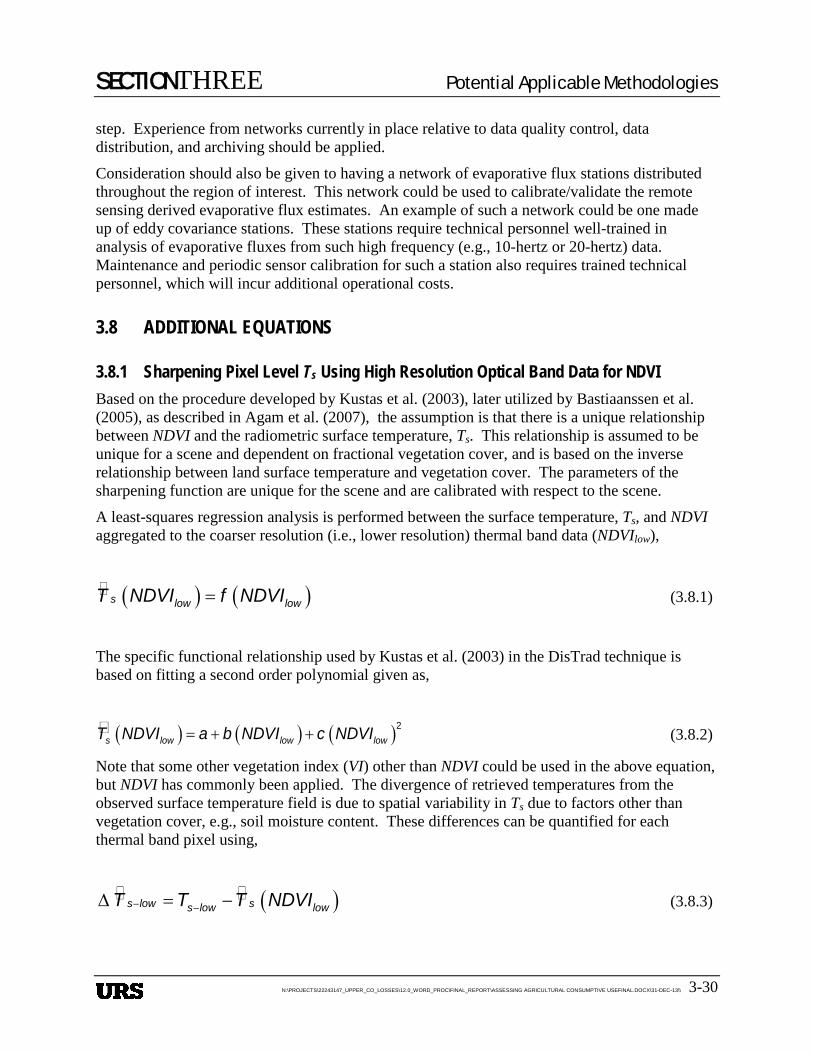
SECTIONTHREE Potential Applicable Methodologies
N:\PROJECTS\22243147_UPPER_CO_LOSSES\12.0_WORD_PROC\FINAL_REPORT\ASSESSING AGRICULTURAL CONSUMPTIVE USEFINAL.DOCX\31-DEC-13\\ 3-30
step. Experience from networks currently in place relative to data quality control, data distribution, and archiving should be applied.
Consideration should also be given to having a network of evaporative flux stations distributed throughout the region of interest. This network could be used to calibrate/validate the remote sensing derived evaporative flux estimates. An example of such a network could be one made up of eddy covariance stations. These stations require technical personnel well-trained in analysis of evaporative fluxes from such high frequency (e.g., 10-hertz or 20-hertz) data. Maintenance and periodic sensor calibration for such a station also requires trained technical personnel, which will incur additional operational costs.
ADDITIONAL EQUATIONS 3.8
3.8.1 Sharpening Pixel Level Ts Using High Resolution Optical Band Data for NDVI Based on the procedure developed by Kustas et al. (2003), later utilized by Bastiaanssen et al. (2005), as described in Agam et al. (2007), the assumption is that there is a unique relationship between NDVI and the radiometric surface temperature, Ts. This relationship is assumed to be unique for a scene and dependent on fractional vegetation cover, and is based on the inverse relationship between land surface temperature and vegetation cover. The parameters of the sharpening function are unique for the scene and are calibrated with respect to the scene.
A least-squares regression analysis is performed between the surface temperature, Ts, and NDVI aggregated to the coarser resolution (i.e., lower resolution) thermal band data (NDVIlow),
( ) ( )=s low lowT NDVI f NDVI (3.8.1)
The specific functional relationship used by Kustas et al. (2003) in the DisTrad technique is based on fitting a second order polynomial given as,
( ) ( ) ( )2s low low lowT NDVI a b NDVI c NDVI= + + (3.8.2)
Note that some other vegetation index (VI) other than NDVI could be used in the above equation, but NDVI has commonly been applied. The divergence of retrieved temperatures from the observed surface temperature field is due to spatial variability in Ts due to factors other than vegetation cover, e.g., soil moisture content. These differences can be quantified for each thermal band pixel using,
( )− −∆ = −s low ss low lowT T T NDVI (3.8.3)
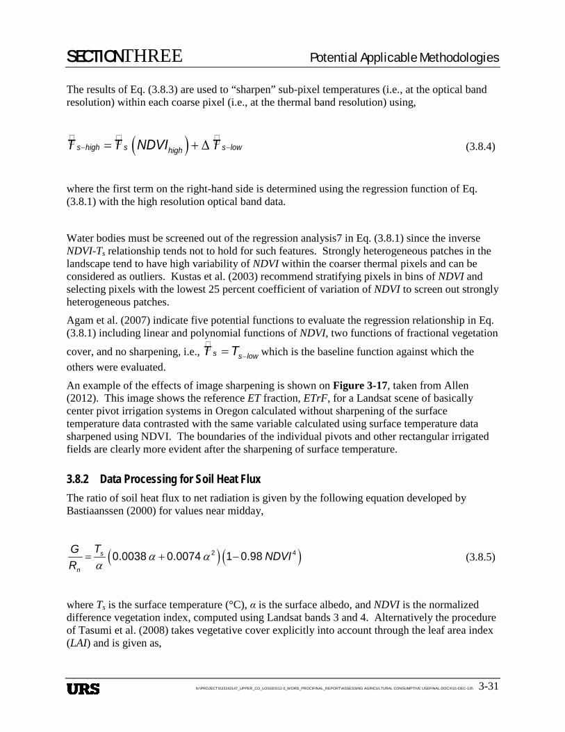
SECTIONTHREE Potential Applicable Methodologies
N:\PROJECTS\22243147_UPPER_CO_LOSSES\12.0_WORD_PROC\FINAL_REPORT\ASSESSING AGRICULTURAL CONSUMPTIVE USEFINAL.DOCX\31-DEC-13\\ 3-31
The results of Eq. (3.8.3) are used to “sharpen” sub-pixel temperatures (i.e., at the optical band resolution) within each coarse pixel (i.e., at the thermal band resolution) using,
( ) − −= + ∆s high s s lowhighT T NDVI T (3.8.4)
where the first term on the right-hand side is determined using the regression function of Eq. (3.8.1) with the high resolution optical band data.
Water bodies must be screened out of the regression analysis7 in Eq. (3.8.1) since the inverse NDVI-Ts relationship tends not to hold for such features. Strongly heterogeneous patches in the landscape tend to have high variability of NDVI within the coarser thermal pixels and can be considered as outliers. Kustas et al. (2003) recommend stratifying pixels in bins of NDVI and selecting pixels with the lowest 25 percent coefficient of variation of NDVI to screen out strongly heterogeneous patches.
Agam et al. (2007) indicate five potential functions to evaluate the regression relationship in Eq. (3.8.1) including linear and polynomial functions of NDVI, two functions of fractional vegetation
cover, and no sharpening, i.e., −=s s lowT T which is the baseline function against which the others were evaluated.
An example of the effects of image sharpening is shown on Figure 3-17, taken from Allen (2012). This image shows the reference ET fraction, ETrF, for a Landsat scene of basically center pivot irrigation systems in Oregon calculated without sharpening of the surface temperature data contrasted with the same variable calculated using surface temperature data sharpened using NDVI. The boundaries of the individual pivots and other rectangular irrigated fields are clearly more evident after the sharpening of surface temperature.
3.8.2 Data Processing for Soil Heat Flux The ratio of soil heat flux to net radiation is given by the following equation developed by Bastiaanssen (2000) for values near midday,
( ) ( )2 40.0038 0.0074 1 0.98s
n
TG NDVIR
α αα
= + − (3.8.5)
where Ts is the surface temperature (°C), α is the surface albedo, and NDVI is the normalized difference vegetation index, computed using Landsat bands 3 and 4. Alternatively the procedure of Tasumi et al. (2008) takes vegetative cover explicitly into account through the leaf area index (LAI) and is given as,
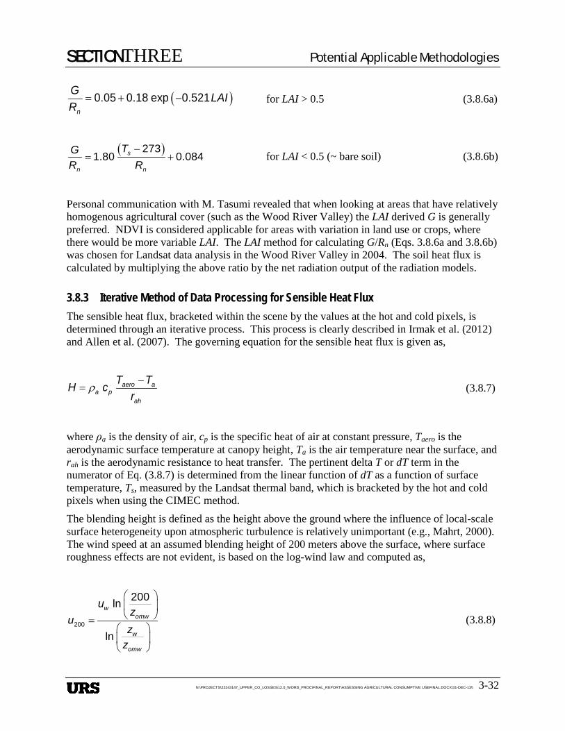
SECTIONTHREE Potential Applicable Methodologies
N:\PROJECTS\22243147_UPPER_CO_LOSSES\12.0_WORD_PROC\FINAL_REPORT\ASSESSING AGRICULTURAL CONSUMPTIVE USEFINAL.DOCX\31-DEC-13\\ 3-32
( )0.05 0.18 exp 0.521n
G LAIR
= + − for LAI > 0.5 (3.8.6a)
( )2731.80 0.084s
n n
TGR R
−= + for LAI < 0.5 (~ bare soil) (3.8.6b)
Personal communication with M. Tasumi revealed that when looking at areas that have relatively homogenous agricultural cover (such as the Wood River Valley) the LAI derived G is generally preferred. NDVI is considered applicable for areas with variation in land use or crops, where there would be more variable LAI. The LAI method for calculating G/Rn (Eqs. 3.8.6a and 3.8.6b) was chosen for Landsat data analysis in the Wood River Valley in 2004. The soil heat flux is calculated by multiplying the above ratio by the net radiation output of the radiation models.
3.8.3 Iterative Method of Data Processing for Sensible Heat Flux The sensible heat flux, bracketed within the scene by the values at the hot and cold pixels, is determined through an iterative process. This process is clearly described in Irmak et al. (2012) and Allen et al. (2007). The governing equation for the sensible heat flux is given as,
aero aa p
ah
T TH cr
ρ−
= (3.8.7)
where ρa is the density of air, cp is the specific heat of air at constant pressure, Taero is the aerodynamic surface temperature at canopy height, Ta is the air temperature near the surface, and rah is the aerodynamic resistance to heat transfer. The pertinent delta T or dT term in the numerator of Eq. (3.8.7) is determined from the linear function of dT as a function of surface temperature, Ts, measured by the Landsat thermal band, which is bracketed by the hot and cold pixels when using the CIMEC method.
The blending height is defined as the height above the ground where the influence of local-scale surface heterogeneity upon atmospheric turbulence is relatively unimportant (e.g., Mahrt, 2000). The wind speed at an assumed blending height of 200 meters above the surface, where surface roughness effects are not evident, is based on the log-wind law and computed as,
200
200ln
ln
womw
w
omw
uz
uz
z
=
(3.8.8)

SECTIONTHREE Potential Applicable Methodologies
N:\PROJECTS\22243147_UPPER_CO_LOSSES\12.0_WORD_PROC\FINAL_REPORT\ASSESSING AGRICULTURAL CONSUMPTIVE USEFINAL.DOCX\31-DEC-13\\ 3-33
where uw is the wind speed measured at weather station height zw, and zomw is the roughness length for the weather station surface.
The shear velocity, *u , for the first iteration (representing neutral stability) evaluated at the blending height of 200 meters is computed as,
200* 200ln
om
k uu
z
=
(3.8.9)
where k is the von Kármán constant (0.41) and zom is the roughness length for momentum, which is a function of canopy height. The aerodynamic resistance for the first iteration, again representing neutral stability, is computed as,
2
1
*
ln
ah
zz
rk u
= (3.8.10)
where z1 and z2 are heights above the zero-plane displacement of the vegetation where the endpoints of dT are defined. Note that these heights of integration are normally taken as z1 = 0.1 m and z2 = 2 m. The initial value of H (representing neutral stability) for each pixel is then computed using Eq. (3.8.7). This initial value of H is used in the calculation of the Monin-Obukhov length, L, which is a function of atmospheric stability,
3*air p sc u T
Lk g H
ρ= − (3.8.11)
where g is the acceleration of gravity. Values of L < 0 indicate an unstable atmospheric boundary layer (i.e., typical daytime conditions) and values of L > 0 indicate stable conditions (i.e., typical nighttime conditions). The stability corrections for momentum (m) and heat transport (h) are computed as a function of the Monin-Obukhov L using the Paulson [1970] and Webb [1970] formulations. For L < 0 (unstable),
( )( ) ( )
( )( )2
200 200200 200
1 12 ln ln 2 arctan 0.5
2 2m m
m m m
x xxΨ π
+ + = + − +
(3.8.12)

SECTIONTHREE Potential Applicable Methodologies
N:\PROJECTS\22243147_UPPER_CO_LOSSES\12.0_WORD_PROC\FINAL_REPORT\ASSESSING AGRICULTURAL CONSUMPTIVE USEFINAL.DOCX\31-DEC-13\\ 3-34
( )( )22
2
12 ln
2m
h m
xΨ
+ =
(3.8.13a)
( )( )20.1
0.1
12 ln
2m
h m
xΨ
+ =
(3.8.13b)
where
( )
0.25
2002001 16mxL
= −
(3.8.14a)
( )
0.25
221 16mxL
= −
(3.8.14b)
( )
0.25
0.10.11 16mxL
= −
(3.8.14c)
When L ≥ 0 values for x(200m), x(2m) and x(0.1m) have no meaning and are set to 1.0. For L > 0 (stable conditions),
( )20025m m L
Ψ = −
(3.8.15)
( )225h m L
Ψ = −
(3.8.16a)
( )0.10.15h m L
Ψ = −
(3.8.16b)

SECTIONTHREE Potential Applicable Methodologies
N:\PROJECTS\22243147_UPPER_CO_LOSSES\12.0_WORD_PROC\FINAL_REPORT\ASSESSING AGRICULTURAL CONSUMPTIVE USEFINAL.DOCX\31-DEC-13\\ 3-35
These stability corrections are then applied to the computation of the shear velocity, *u , and aerodynamic resistance, rah, for non-neutral conditions as follows,
( )
200*
2000
200ln m mm
k uu
zΨ
=
−
(3.8.17)
( ) ( )2 1
2
1
*
ln h z h z
ah
zz
rk u
Ψ Ψ
− + = (3.8.18)
This new value of rah is used to solve for an updated value of H in Eq. (3.8.7). These iterations are continued until successive values for the sensible heat flux H and/or the Monin-Obukhov L are within a prescribed closure criteria.
3.8.4 Cost Estimates of Eddy Covariance and Micrometeorological Stations A cost estimate for a combined eddy covariance, energy balance and micrometeorological station is given in Table 3.12. A cost estimate for eddy covariance network support is given in Table 3.13. Note that only one of each item in Table 3.13 is needed for each network, e.g. for each state or each region. A cost estimate for a reference ET monitoring station is given in Table 3.14. All of these cost estimates are based on recent quotes from Campbell Scientific, Inc. and from Licor Corporation. Note that these costs represent only the capital costs for equipment and do not reflect the on-going operational cost of programming, installing, and maintaining stations, or data analysis, quality control, and reporting.
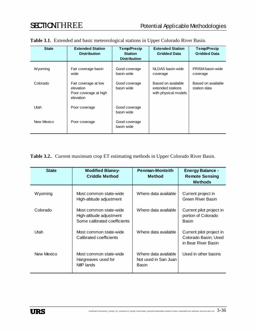
SECTIONTHREE Potential Applicable Methodologies
N:\PROJECTS\22243147_UPPER_CO_LOSSES\12.0_WORD_PROC\FINAL_REPORT\ASSESSING AGRICULTURAL CONSUMPTIVE USEFINAL.DOCX\31-DEC-13\\ 3-36
Table 3.1. Extended and basic meteorological stations in Upper Colorado River Basin.
Table 3.2.. Current maximum crop ET estimating methods in Upper Colorado River Basin.
State Extended Station Temp/Precip Extended Station Temp/PrecipDistribution Station Gridded Data Gridded Data
Distribution
Wyoming Fair coverage basin Good coverage NLDAS basin-wide PRISM basin-widewide basin wide coverage coverage
Colorado Fair coverage at low Good coverage Based on available Based on available elevation basin wide extended stations station dataPoor coverage at high with physical modelselevation
Utah Poor coverage Good coveragebasin wide
New Mexico Poor coverage Good coveragebasin wide
State Modified Blaney- Penman-Monteith Energy Balance - Criddle Method Method Remote Sensing
Methods
Wyoming Most common state-wide Where data available Current project inHigh-altitude adjustment Green River Basin
Colorado Most common state-wide Where data available Current pilot project inHigh-altitude adjustment portion of Colorado Some calibrated coefficients Basin
Utah Most common state-wide Where data available Current pilot project inCalibrated coefficients Colorado Basin; Used
in Bear River Basin
New Mexico Most common state-wide Where data available Used in other basinsHargreaves used for Not used in San JuanNIIP lands Basin
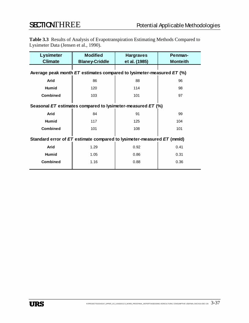
SECTIONTHREE Potential Applicable Methodologies
N:\PROJECTS\22243147_UPPER_CO_LOSSES\12.0_WORD_PROC\FINAL_REPORT\ASSESSING AGRICULTURAL CONSUMPTIVE USEFINAL.DOCX\31-DEC-13\\ 3-37
Table 3.3 Results of Analysis of Evapotranspiration Estimating Methods Compared to Lysimeter Data (Jensen et al., 1990).
Lysimeter Modified Hargraves Penman-Climate Blaney-Criddle et al. (1985) Monteith
Average peak month ET estimates compared to lysimeter-measured ET (%)Arid 86 88 96
Humid 120 114 98
Combined 103 101 97
Seasonal ET estimates compared to lysimeter-measured ET (%)Arid 84 91 99
Humid 117 125 104
Combined 101 108 101
Standard error of ET estimate compared to lysimeter-measured ET (mm/d)Arid 1.29 0.92 0.41
Humid 1.05 0.86 0.31
Combined 1.16 0.88 0.36
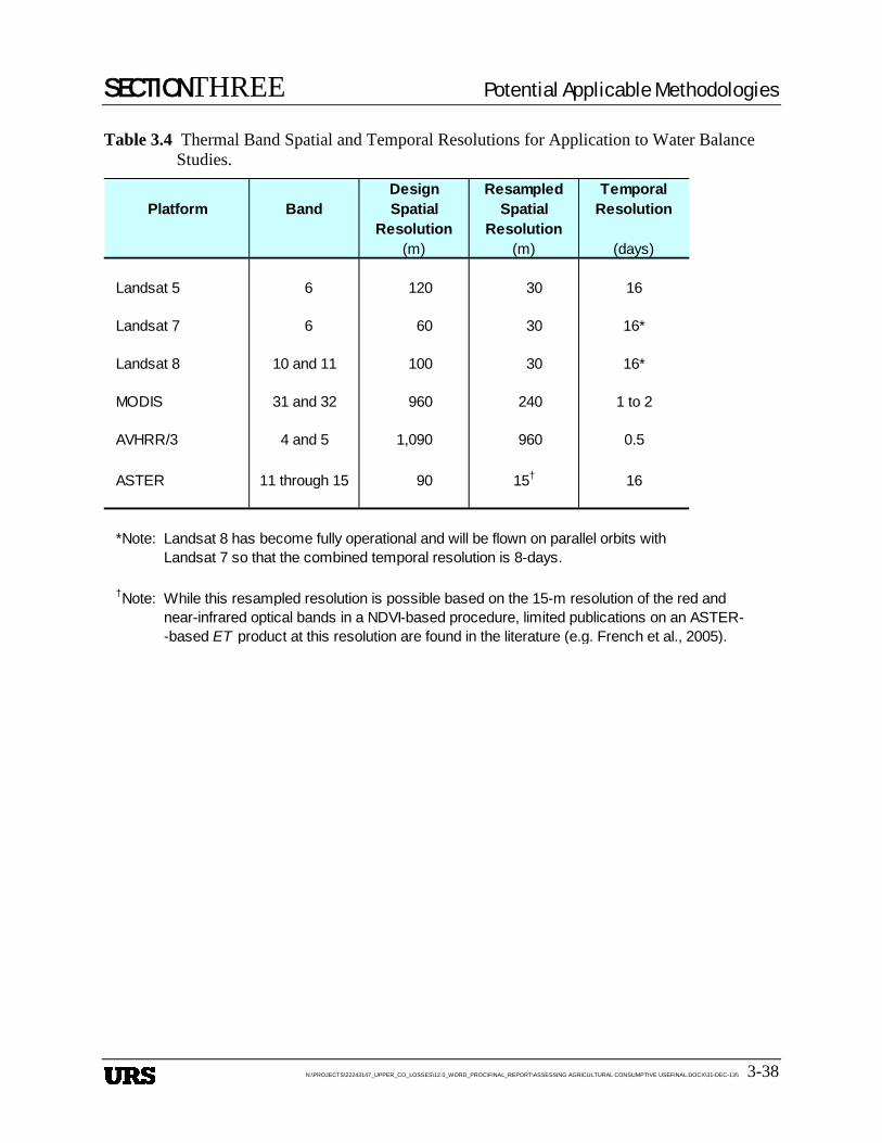
SECTIONTHREE Potential Applicable Methodologies
N:\PROJECTS\22243147_UPPER_CO_LOSSES\12.0_WORD_PROC\FINAL_REPORT\ASSESSING AGRICULTURAL CONSUMPTIVE USEFINAL.DOCX\31-DEC-13\\ 3-38
Table 3.4 Thermal Band Spatial and Temporal Resolutions for Application to Water Balance Studies.
Design Resampled TemporalPlatform Band Spatial Spatial Resolution
Resolution Resolution(m) (m) (days)
Landsat 5 6 120 30 16
Landsat 7 6 60 30 16*
Landsat 8 10 and 11 100 30 16*
MODIS 31 and 32 960 240 1 to 2
AVHRR/3 4 and 5 1,090 960 0.5
ASTER 11 through 15 90 15† 16
*Note: Landsat 8 has become fully operational and will be flown on parallel orbits with Landsat 7 so that the combined temporal resolution is 8-days.
†Note: While this resampled resolution is possible based on the 15-m resolution of the red and near-infrared optical bands in a NDVI-based procedure, limited publications on an ASTER- -based ET product at this resolution are found in the literature (e.g. French et al., 2005).
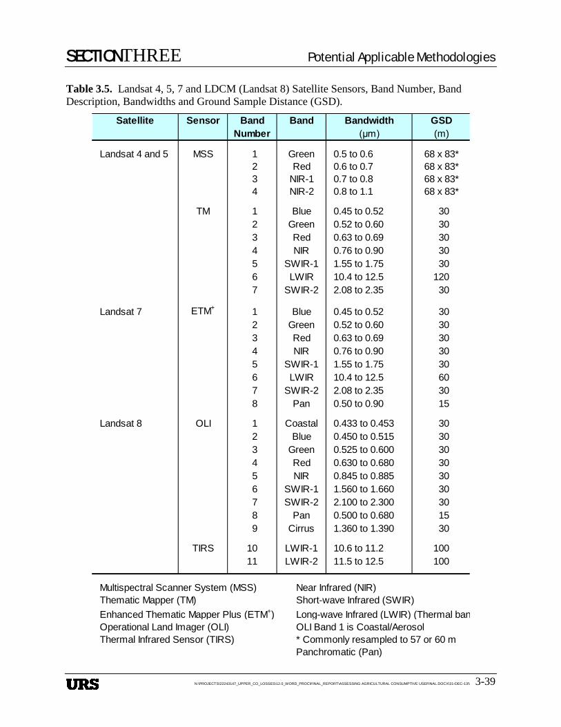
SECTIONTHREE Potential Applicable Methodologies
N:\PROJECTS\22243147_UPPER_CO_LOSSES\12.0_WORD_PROC\FINAL_REPORT\ASSESSING AGRICULTURAL CONSUMPTIVE USEFINAL.DOCX\31-DEC-13\\ 3-39
Table 3.5. Landsat 4, 5, 7 and LDCM (Landsat 8) Satellite Sensors, Band Number, Band Description, Bandwidths and Ground Sample Distance (GSD).
Satellite Sensor Band Band Bandwidth GSDNumber (μm) (m)
Landsat 4 and 5 MSS 1 Green 0.5 to 0.6 68 x 83*2 Red 0.6 to 0.7 68 x 83*3 NIR-1 0.7 to 0.8 68 x 83*4 NIR-2 0.8 to 1.1 68 x 83*
TM 1 Blue 0.45 to 0.52 302 Green 0.52 to 0.60 303 Red 0.63 to 0.69 304 NIR 0.76 to 0.90 305 SWIR-1 1.55 to 1.75 306 LWIR 10.4 to 12.5 1207 SWIR-2 2.08 to 2.35 30
Landsat 7 ETM+ 1 Blue 0.45 to 0.52 302 Green 0.52 to 0.60 303 Red 0.63 to 0.69 304 NIR 0.76 to 0.90 305 SWIR-1 1.55 to 1.75 306 LWIR 10.4 to 12.5 607 SWIR-2 2.08 to 2.35 308 Pan 0.50 to 0.90 15
Landsat 8 OLI 1 Coastal 0.433 to 0.453 302 Blue 0.450 to 0.515 303 Green 0.525 to 0.600 304 Red 0.630 to 0.680 305 NIR 0.845 to 0.885 306 SWIR-1 1.560 to 1.660 307 SWIR-2 2.100 to 2.300 308 Pan 0.500 to 0.680 159 Cirrus 1.360 to 1.390 30
TIRS 10 LWIR-1 10.6 to 11.2 10011 LWIR-2 11.5 to 12.5 100
Multispectral Scanner System (MSS) Near Infrared (NIR)Thematic Mapper (TM) Short-wave Infrared (SWIR)Enhanced Thematic Mapper Plus (ETM+) Long-wave Infrared (LWIR) (Thermal banOperational Land Imager (OLI) OLI Band 1 is Coastal/AerosolThermal Infrared Sensor (TIRS) * Commonly resampled to 57 or 60 m
Panchromatic (Pan)
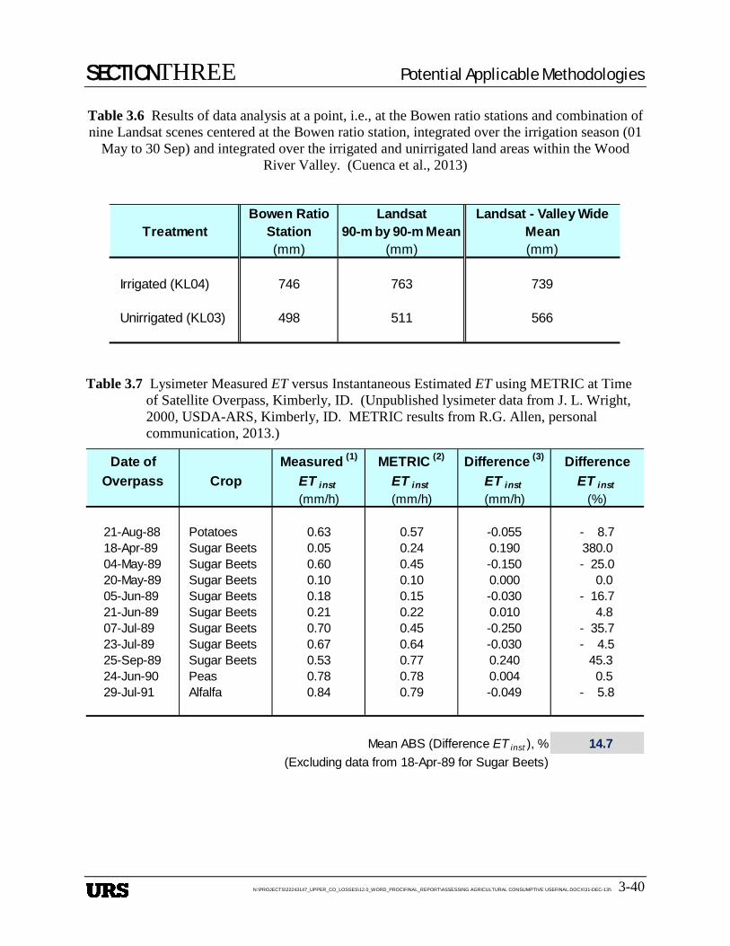
SECTIONTHREE Potential Applicable Methodologies
N:\PROJECTS\22243147_UPPER_CO_LOSSES\12.0_WORD_PROC\FINAL_REPORT\ASSESSING AGRICULTURAL CONSUMPTIVE USEFINAL.DOCX\31-DEC-13\\ 3-40
Table 3.6 Results of data analysis at a point, i.e., at the Bowen ratio stations and combination of nine Landsat scenes centered at the Bowen ratio station, integrated over the irrigation season (01
May to 30 Sep) and integrated over the irrigated and unirrigated land areas within the Wood River Valley. (Cuenca et al., 2013)
Table 3.7 Lysimeter Measured ET versus Instantaneous Estimated ET using METRIC at Time of Satellite Overpass, Kimberly, ID. (Unpublished lysimeter data from J. L. Wright, 2000, USDA-ARS, Kimberly, ID. METRIC results from R.G. Allen, personal communication, 2013.)
Bowen Ratio Landsat Landsat - Valley WideTreatment Station 90-m by 90-m Mean Mean
(mm) (mm) (mm)
Irrigated (KL04) 746 763 739
Unirrigated (KL03) 498 511 566
Date of Measured (1) METRIC (2) Difference (3) DifferenceOverpass Crop ET inst ET inst ET inst ET inst
(mm/h) (mm/h) (mm/h) (%)
21-Aug-88 Potatoes 0.63 0.57 -0.055 - 8.718-Apr-89 Sugar Beets 0.05 0.24 0.190 380.004-May-89 Sugar Beets 0.60 0.45 -0.150 - 25.020-May-89 Sugar Beets 0.10 0.10 0.000 0.005-Jun-89 Sugar Beets 0.18 0.15 -0.030 - 16.721-Jun-89 Sugar Beets 0.21 0.22 0.010 4.807-Jul-89 Sugar Beets 0.70 0.45 -0.250 - 35.723-Jul-89 Sugar Beets 0.67 0.64 -0.030 - 4.525-Sep-89 Sugar Beets 0.53 0.77 0.240 45.324-Jun-90 Peas 0.78 0.78 0.004 0.529-Jul-91 Alfalfa 0.84 0.79 -0.049 - 5.8
Mean ABS (Difference ET inst ), % 14.7(Excluding data from 18-Apr-89 for Sugar Beets)
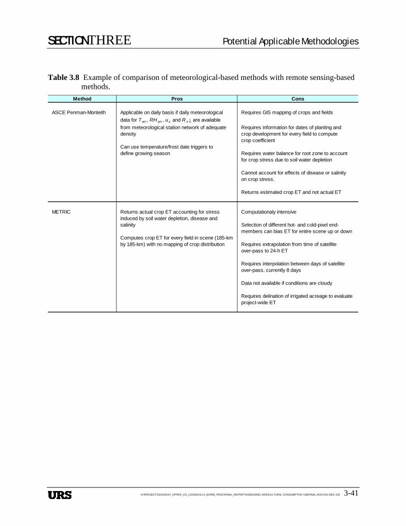
SECTIONTHREE Potential Applicable Methodologies
N:\PROJECTS\22243147_UPPER_CO_LOSSES\12.0_WORD_PROC\FINAL_REPORT\ASSESSING AGRICULTURAL CONSUMPTIVE USEFINAL.DOCX\31-DEC-13\\ 3-41
Table 3.8 Example of comparison of meteorological-based methods with remote sensing-based methods.
Method Pros Cons
ASCE Penman-Monteith Applicable on daily basis if daily meteorological Requires GIS mapping of crops and fieldsdata for T air , RH air , uz and R s ↓ are available from meteorological station network of adequate Requires information for dates of planting and density crop development for every field to compute
crop coefficientCan use temperature/frost date triggers to define growing season Requires water balance for root zone to account
for crop stress due to soil water depletion
Cannot account for effects of disease or salinity on crop stress.
Returns estimated crop ET and not actual ET
METRIC Returns actual crop ET accounting for stress Computationaly intensiveinduced by soil water depletion, disease andsalinity Selection of different hot- and cold-pixel end-
members can bias ET for entire scene up or downComputes crop ET for every field in scene (185-kmby 185-km) with no mapping of crop distribution Requires extrapolation from time of satellite
over-pass to 24-h ET
Requires interpolation between days of satelliteover-pass, currently 8 days
Data not available if conditions are cloudy
Requires delination of irrigated acreage to evaluate project-wide ET
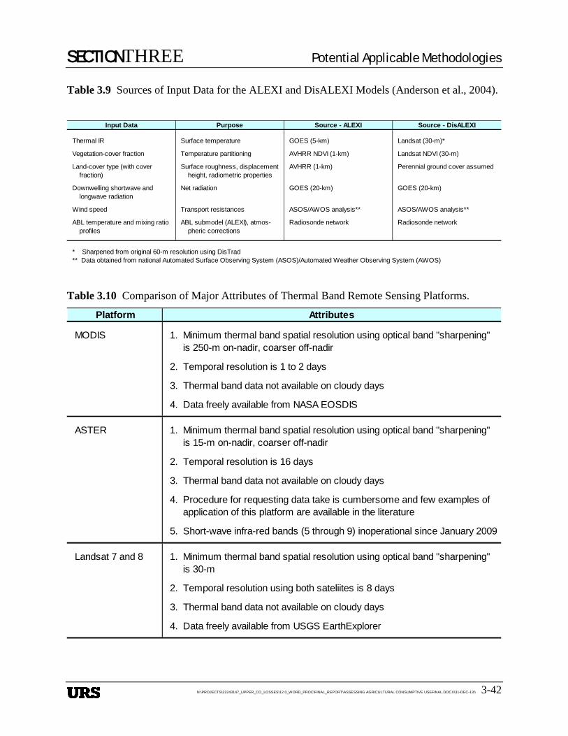
SECTIONTHREE Potential Applicable Methodologies
N:\PROJECTS\22243147_UPPER_CO_LOSSES\12.0_WORD_PROC\FINAL_REPORT\ASSESSING AGRICULTURAL CONSUMPTIVE USEFINAL.DOCX\31-DEC-13\\ 3-42
Table 3.9 Sources of Input Data for the ALEXI and DisALEXI Models (Anderson et al., 2004).
Table 3.10 Comparison of Major Attributes of Thermal Band Remote Sensing Platforms.
Input Data Purpose Source - ALEXI Source - DisALEXI
Thermal IR Surface temperature GOES (5-km) Landsat (30-m)*
Vegetation-cover fraction Temperature partitioning AVHRR NDVI (1-km) Landsat NDVI (30-m)
Land-cover type (with cover Surface roughness, displacement AVHRR (1-km) Perennial ground cover assumed fraction) height, radiometric properties
Downwelling shortwave and Net radiation GOES (20-km) GOES (20-km) longwave radiation
Wind speed Transport resistances ASOS/AWOS analysis** ASOS/AWOS analysis**
ABL temperature and mixing ratio ABL submodel (ALEXI), atmos- Radiosonde network Radiosonde network profiles pheric corrections
* Sharpened from original 60-m resolution using DisTrad** Data obtained from national Automated Surface Observing System (ASOS)/Automated Weather Observing System (AWOS)
Platform Attributes
MODIS 1. Minimum thermal band spatial resolution using optical band "sharpening" is 250-m on-nadir, coarser off-nadir
2. Temporal resolution is 1 to 2 days
3. Thermal band data not available on cloudy days
4. Data freely available from NASA EOSDIS
ASTER 1. Minimum thermal band spatial resolution using optical band "sharpening" is 15-m on-nadir, coarser off-nadir
2. Temporal resolution is 16 days
3. Thermal band data not available on cloudy days
4. Procedure for requesting data take is cumbersome and few examples of application of this platform are available in the literature
5. Short-wave infra-red bands (5 through 9) inoperational since January 2009
Landsat 7 and 8 1. Minimum thermal band spatial resolution using optical band "sharpening" is 30-m
2. Temporal resolution using both sateliites is 8 days
3. Thermal band data not available on cloudy days
4. Data freely available from USGS EarthExplorer
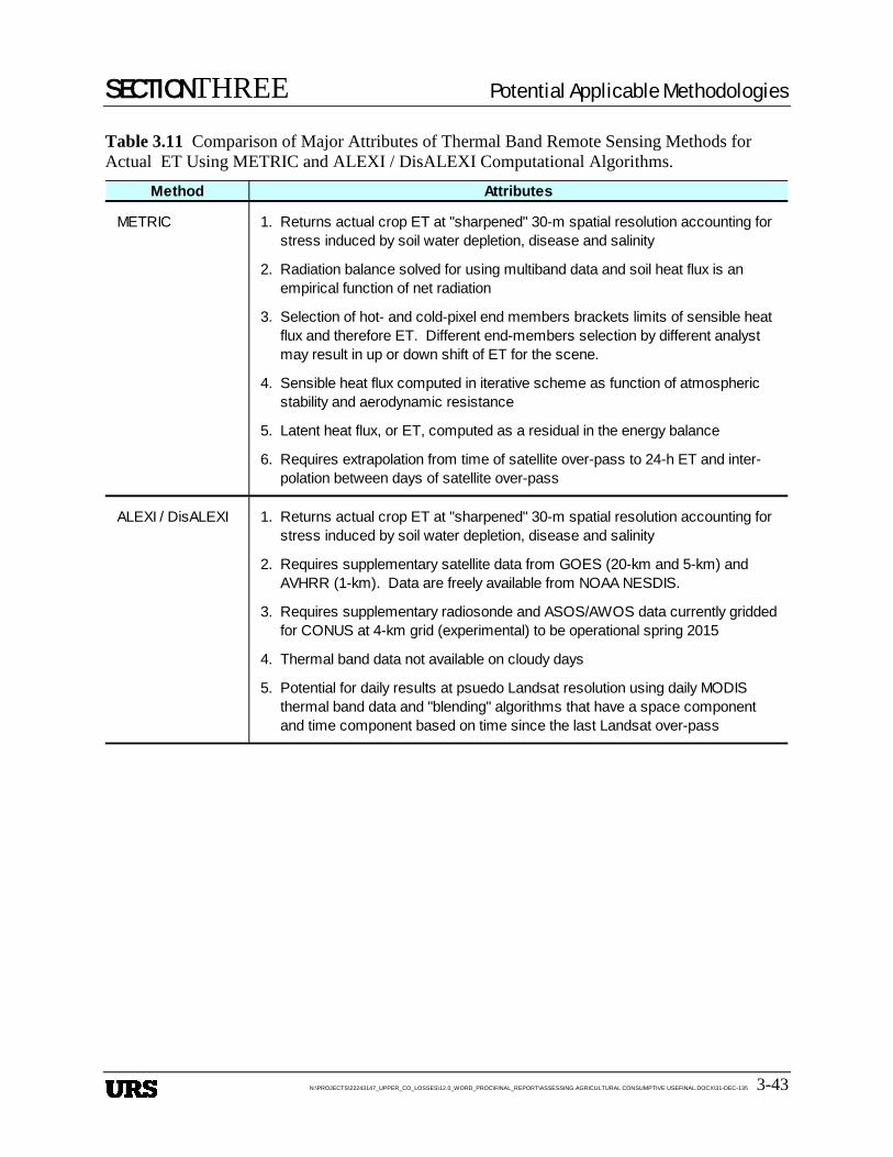
SECTIONTHREE Potential Applicable Methodologies
N:\PROJECTS\22243147_UPPER_CO_LOSSES\12.0_WORD_PROC\FINAL_REPORT\ASSESSING AGRICULTURAL CONSUMPTIVE USEFINAL.DOCX\31-DEC-13\\ 3-43
Table 3.11 Comparison of Major Attributes of Thermal Band Remote Sensing Methods for Actual ET Using METRIC and ALEXI / DisALEXI Computational Algorithms.
Method Attributes
METRIC 1. Returns actual crop ET at "sharpened" 30-m spatial resolution accounting for stress induced by soil water depletion, disease and salinity
2. Radiation balance solved for using multiband data and soil heat flux is an empirical function of net radiation
3. Selection of hot- and cold-pixel end members brackets limits of sensible heat flux and therefore ET. Different end-members selection by different analyst may result in up or down shift of ET for the scene.
4. Sensible heat flux computed in iterative scheme as function of atmospheric stability and aerodynamic resistance
5. Latent heat flux, or ET, computed as a residual in the energy balance
6. Requires extrapolation from time of satellite over-pass to 24-h ET and inter- polation between days of satellite over-pass
ALEXI / DisALEXI 1. Returns actual crop ET at "sharpened" 30-m spatial resolution accounting for stress induced by soil water depletion, disease and salinity
2. Requires supplementary satellite data from GOES (20-km and 5-km) and AVHRR (1-km). Data are freely available from NOAA NESDIS.
3. Requires supplementary radiosonde and ASOS/AWOS data currently gridded for CONUS at 4-km grid (experimental) to be operational spring 2015
4. Thermal band data not available on cloudy days
5. Potential for daily results at psuedo Landsat resolution using daily MODIS thermal band data and "blending" algorithms that have a space component and time component based on time since the last Landsat over-pass
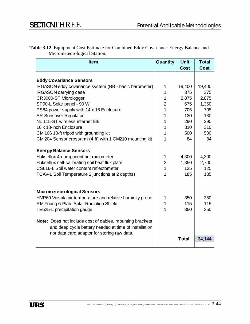
SECTIONTHREE Potential Applicable Methodologies
N:\PROJECTS\22243147_UPPER_CO_LOSSES\12.0_WORD_PROC\FINAL_REPORT\ASSESSING AGRICULTURAL CONSUMPTIVE USEFINAL.DOCX\31-DEC-13\\ 3-44
Table 3.12 Equipment Cost Estimate for Combined Eddy Covariance-Energy Balance and Micrometeorological Station.
Item Quantity Unit TotalCost Cost
Eddy Covariance SensorsIRGASON eddy covariance system (BB - basic barometer) 1 19,400 19,400IRGASON carrying case 1 375 375CR3000-ST Micrologger 1 2,875 2,875SP90-L Solar panel - 90 W 2 675 1,350PS84 power supply with 14 x 16 Enclosure 1 705 705SR Sunsaver Regulator 1 130 130NL 115-ST wireless internet link 1 290 29016 x 18-inch Enclosure 1 310 310CM 106 10-ft tripod with grounding kit 1 500 500CM 204 Sensor crossarm (4-ft) with 1 CM210 mounting kit 1 84 84
Energy Balance SensorsHukseflux 4-component net radiometer 1 4,300 4,300Hukseflux self-calibrating soil heat flux plate 2 1,350 2,700CS616-L Soil water content reflectometer 1 125 125TCAV-L Soil Temperature 2 junctions at 2 depths) 1 185 185
Micrometeorological SensorsHMP60 Vaisala air temperature and relative humidity probe 1 350 350RM Young 6-Plate Solar Radiation Shield 1 115 115TE525-L precipitation gauge 1 350 350
Note: Does not include cost of cables, mounting brackets and deep cycle battery needed at time of installation nor data card adaptor for storing raw data.
Total 34,144
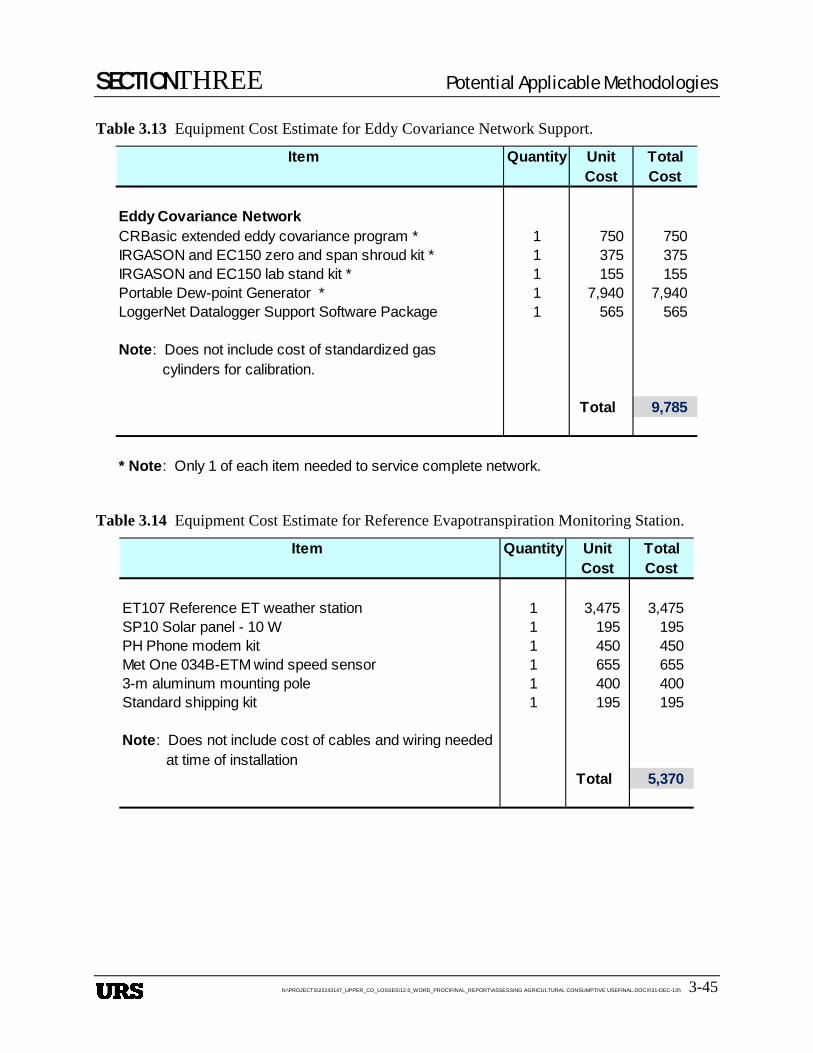
SECTIONTHREE Potential Applicable Methodologies
N:\PROJECTS\22243147_UPPER_CO_LOSSES\12.0_WORD_PROC\FINAL_REPORT\ASSESSING AGRICULTURAL CONSUMPTIVE USEFINAL.DOCX\31-DEC-13\\ 3-45
Table 3.13 Equipment Cost Estimate for Eddy Covariance Network Support.
Table 3.14 Equipment Cost Estimate for Reference Evapotranspiration Monitoring Station.
Item Quantity Unit TotalCost Cost
Eddy Covariance NetworkCRBasic extended eddy covariance program * 1 750 750IRGASON and EC150 zero and span shroud kit * 1 375 375IRGASON and EC150 lab stand kit * 1 155 155Portable Dew-point Generator * 1 7,940 7,940LoggerNet Datalogger Support Software Package 1 565 565
Note: Does not include cost of standardized gas cylinders for calibration.
Total 9,785
* Note: Only 1 of each item needed to service complete network.
Item Quantity Unit TotalCost Cost
ET107 Reference ET weather station 1 3,475 3,475SP10 Solar panel - 10 W 1 195 195PH Phone modem kit 1 450 450Met One 034B-ETM wind speed sensor 1 655 6553-m aluminum mounting pole 1 400 400Standard shipping kit 1 195 195
Note: Does not include cost of cables and wiring needed at time of installation
Total 5,370
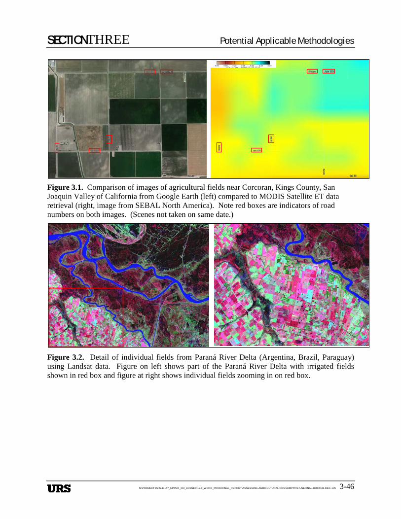
SECTIONTHREE Potential Applicable Methodologies
N:\PROJECTS\22243147_UPPER_CO_LOSSES\12.0_WORD_PROC\FINAL_REPORT\ASSESSING AGRICULTURAL CONSUMPTIVE USEFINAL.DOCX\31-DEC-13\\ 3-46
Figure 3.1. Comparison of images of agricultural fields near Corcoran, Kings County, San Joaquin Valley of California from Google Earth (left) compared to MODIS Satellite ET data retrieval (right, image from SEBAL North America). Note red boxes are indicators of road numbers on both images. (Scenes not taken on same date.)
Figure 3.2. Detail of individual fields from Paraná River Delta (Argentina, Brazil, Paraguay) using Landsat data. Figure on left shows part of the Paraná River Delta with irrigated fields shown in red box and figure at right shows individual fields zooming in on red box.
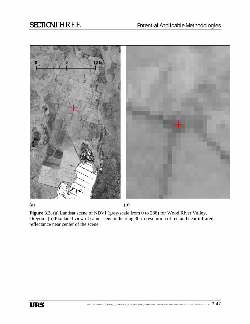
SECTIONTHREE Potential Applicable Methodologies
N:\PROJECTS\22243147_UPPER_CO_LOSSES\12.0_WORD_PROC\FINAL_REPORT\ASSESSING AGRICULTURAL CONSUMPTIVE USEFINAL.DOCX\31-DEC-13\\ 3-47
(a) (b)
Figure 3.3. (a) Landsat scene of NDVI (grey-scale from 0 to 288) for Wood River Valley, Oregon. (b) Pixelated view of same scene indicating 30-m resolution of red and near infrared reflectance near center of the scene.
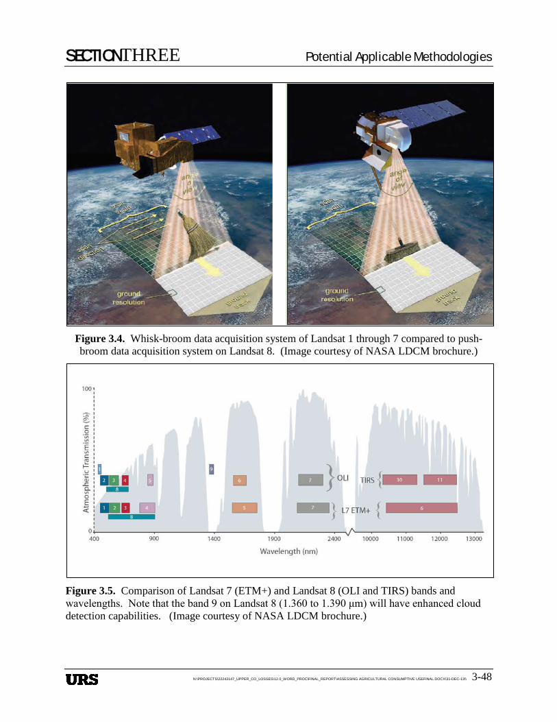
SECTIONTHREE Potential Applicable Methodologies
N:\PROJECTS\22243147_UPPER_CO_LOSSES\12.0_WORD_PROC\FINAL_REPORT\ASSESSING AGRICULTURAL CONSUMPTIVE USEFINAL.DOCX\31-DEC-13\\ 3-48
Figure 3.4. Whisk-broom data acquisition system of Landsat 1 through 7 compared to push-broom data acquisition system on Landsat 8. (Image courtesy of NASA LDCM brochure.)
Figure 3.5. Comparison of Landsat 7 (ETM+) and Landsat 8 (OLI and TIRS) bands and wavelengths. Note that the band 9 on Landsat 8 (1.360 to 1.390 μm) will have enhanced cloud detection capabilities. (Image courtesy of NASA LDCM brochure.)
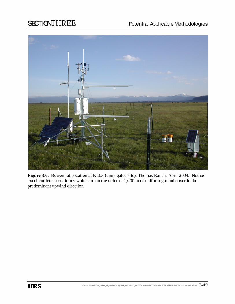
SECTIONTHREE Potential Applicable Methodologies
N:\PROJECTS\22243147_UPPER_CO_LOSSES\12.0_WORD_PROC\FINAL_REPORT\ASSESSING AGRICULTURAL CONSUMPTIVE USEFINAL.DOCX\31-DEC-13\\ 3-49
Figure 3.6. Bowen ratio station at KL03 (unirrigated site), Thomas Ranch, April 2004. Notice excellent fetch conditions which are on the order of 1,000 m of uniform ground cover in the predominant upwind direction.

SECTIONTHREE Potential Applicable Methodologies
N:\PROJECTS\22243147_UPPER_CO_LOSSES\12.0_WORD_PROC\FINAL_REPORT\ASSESSING AGRICULTURAL CONSUMPTIVE USEFINAL.DOCX\31-DEC-13\\ 3-50
Figure 3.7 (a). Energy balance for net radiation (Rnet), soil heat flux (G), sensible heat flux (H), and latent heat flux (or evapotranspiration) (LE) every 20-min measured by the Bowen ratio system at KL03 (unirrigated) site for DOY 288 (14 October) 2004.
Bowen Ratio Station KL03 - Energy Balance - Pasture - 2004
-100
0
100
200
300
400
500
288.0 288.1 288.2 288.3 288.4 288.5 288.6 288.7 288.8 288.9 289.0
DOY
Ener
gy F
lux
(W/m
2 )
Rnet G LE H
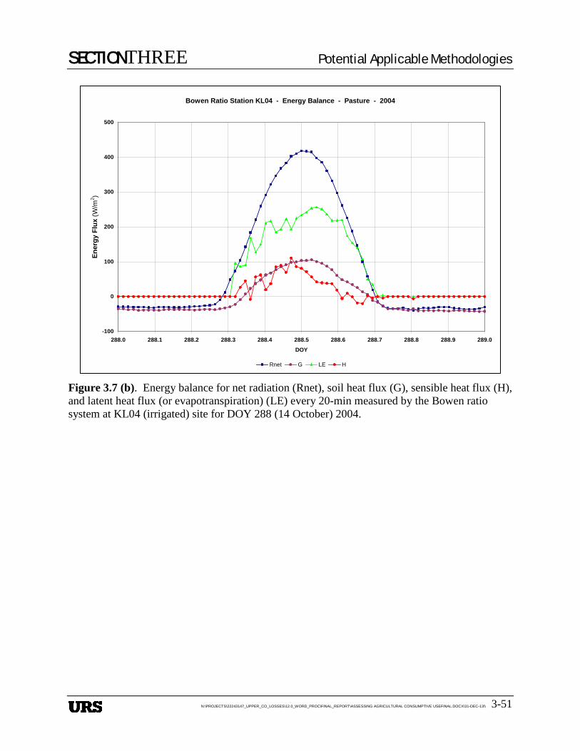
SECTIONTHREE Potential Applicable Methodologies
N:\PROJECTS\22243147_UPPER_CO_LOSSES\12.0_WORD_PROC\FINAL_REPORT\ASSESSING AGRICULTURAL CONSUMPTIVE USEFINAL.DOCX\31-DEC-13\\ 3-51
Figure 3.7 (b). Energy balance for net radiation (Rnet), soil heat flux (G), sensible heat flux (H), and latent heat flux (or evapotranspiration) (LE) every 20-min measured by the Bowen ratio system at KL04 (irrigated) site for DOY 288 (14 October) 2004.
Bowen Ratio Station KL04 - Energy Balance - Pasture - 2004
-100
0
100
200
300
400
500
288.0 288.1 288.2 288.3 288.4 288.5 288.6 288.7 288.8 288.9 289.0
DOY
Ener
gy F
lux
(W/m
2 )
Rnet G LE H
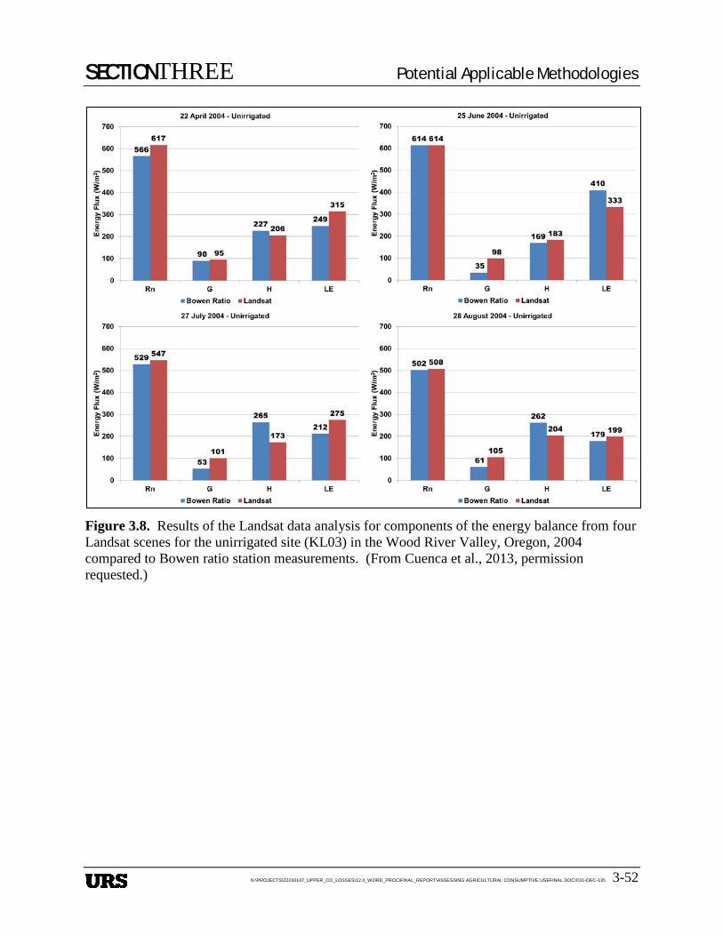
SECTIONTHREE Potential Applicable Methodologies
N:\PROJECTS\22243147_UPPER_CO_LOSSES\12.0_WORD_PROC\FINAL_REPORT\ASSESSING AGRICULTURAL CONSUMPTIVE USEFINAL.DOCX\31-DEC-13\\ 3-52
Figure 3.8. Results of the Landsat data analysis for components of the energy balance from four Landsat scenes for the unirrigated site (KL03) in the Wood River Valley, Oregon, 2004 compared to Bowen ratio station measurements. (From Cuenca et al., 2013, permission requested.)
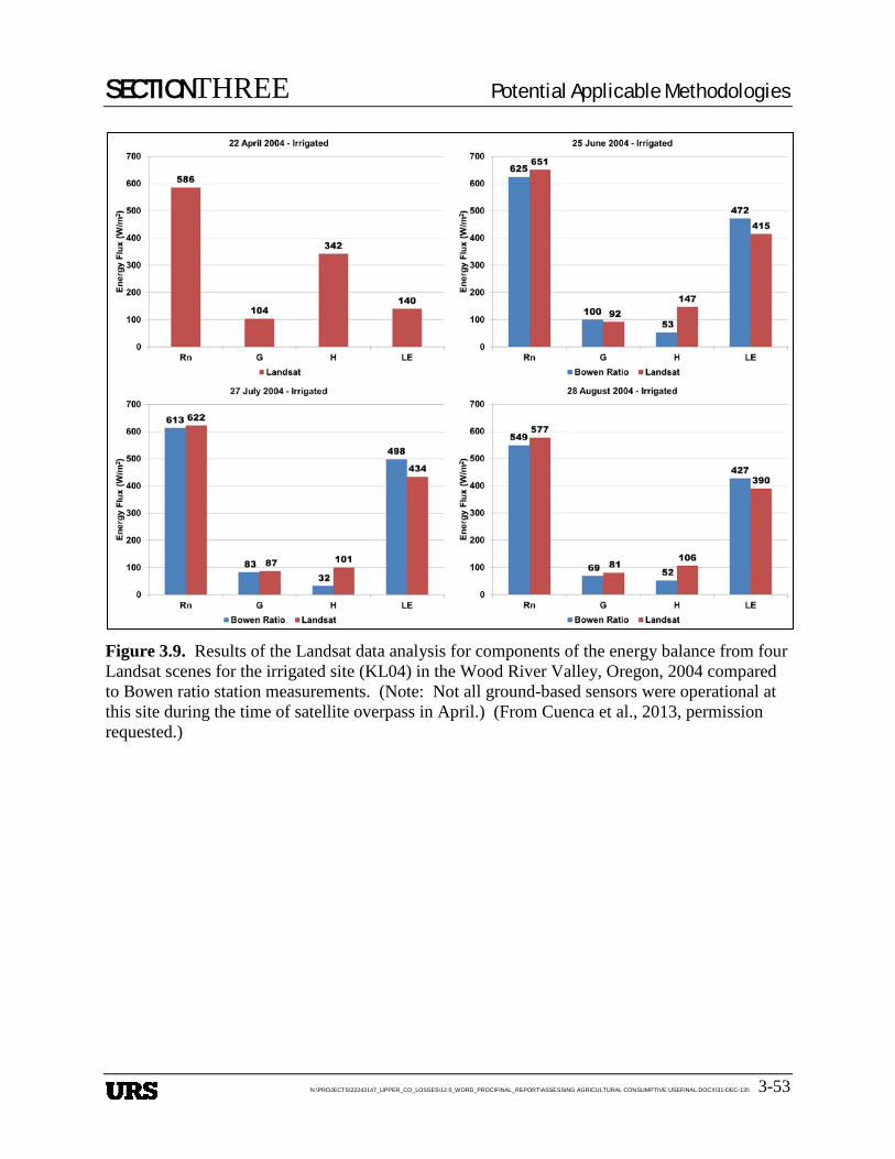
SECTIONTHREE Potential Applicable Methodologies
N:\PROJECTS\22243147_UPPER_CO_LOSSES\12.0_WORD_PROC\FINAL_REPORT\ASSESSING AGRICULTURAL CONSUMPTIVE USEFINAL.DOCX\31-DEC-13\\ 3-53
Figure 3.9. Results of the Landsat data analysis for components of the energy balance from four Landsat scenes for the irrigated site (KL04) in the Wood River Valley, Oregon, 2004 compared to Bowen ratio station measurements. (Note: Not all ground-based sensors were operational at this site during the time of satellite overpass in April.) (From Cuenca et al., 2013, permission requested.)
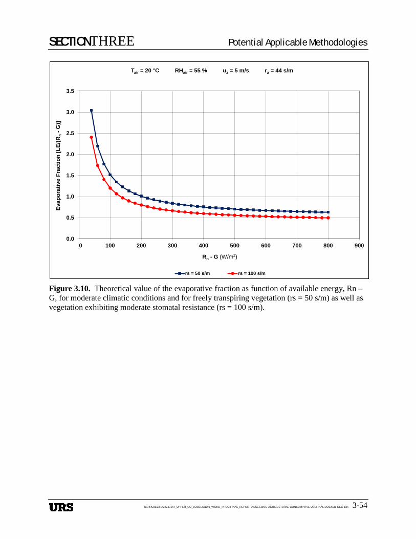
SECTIONTHREE Potential Applicable Methodologies
N:\PROJECTS\22243147_UPPER_CO_LOSSES\12.0_WORD_PROC\FINAL_REPORT\ASSESSING AGRICULTURAL CONSUMPTIVE USEFINAL.DOCX\31-DEC-13\\ 3-54
Figure 3.10. Theoretical value of the evaporative fraction as function of available energy, Rn – G, for moderate climatic conditions and for freely transpiring vegetation (rs = 50 s/m) as well as vegetation exhibiting moderate stomatal resistance (rs = 100 s/m).
0.0
0.5
1.0
1.5
2.0
2.5
3.0
3.5
0 100 200 300 400 500 600 700 800 900
Evap
orat
ive
Frac
tion
[LE/
(Rn
-G)]
Rn - G (W/m2)
Tair = 20 °C RHair = 55 % uz = 5 m/s ra = 44 s/m
rs = 50 s/m rs = 100 s/m
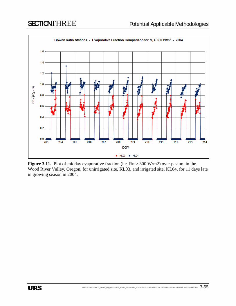
SECTIONTHREE Potential Applicable Methodologies
N:\PROJECTS\22243147_UPPER_CO_LOSSES\12.0_WORD_PROC\FINAL_REPORT\ASSESSING AGRICULTURAL CONSUMPTIVE USEFINAL.DOCX\31-DEC-13\\ 3-55
Figure 3.11. Plot of midday evaporative fraction (i.e. Rn > 300 W/m2) over pasture in the Wood River Valley, Oregon, for unirrigated site, KL03, and irrigated site, KL04, for 11 days late in growing season in 2004.
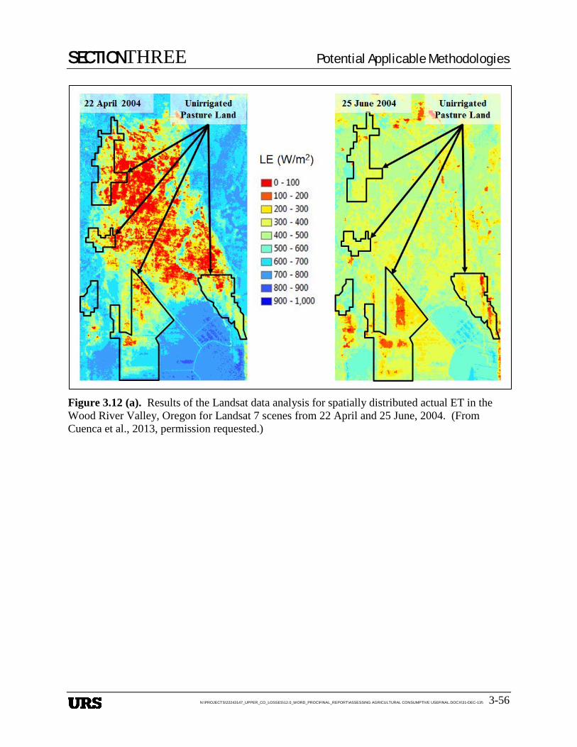
SECTIONTHREE Potential Applicable Methodologies
N:\PROJECTS\22243147_UPPER_CO_LOSSES\12.0_WORD_PROC\FINAL_REPORT\ASSESSING AGRICULTURAL CONSUMPTIVE USEFINAL.DOCX\31-DEC-13\\ 3-56
Figure 3.12 (a). Results of the Landsat data analysis for spatially distributed actual ET in the Wood River Valley, Oregon for Landsat 7 scenes from 22 April and 25 June, 2004. (From Cuenca et al., 2013, permission requested.)
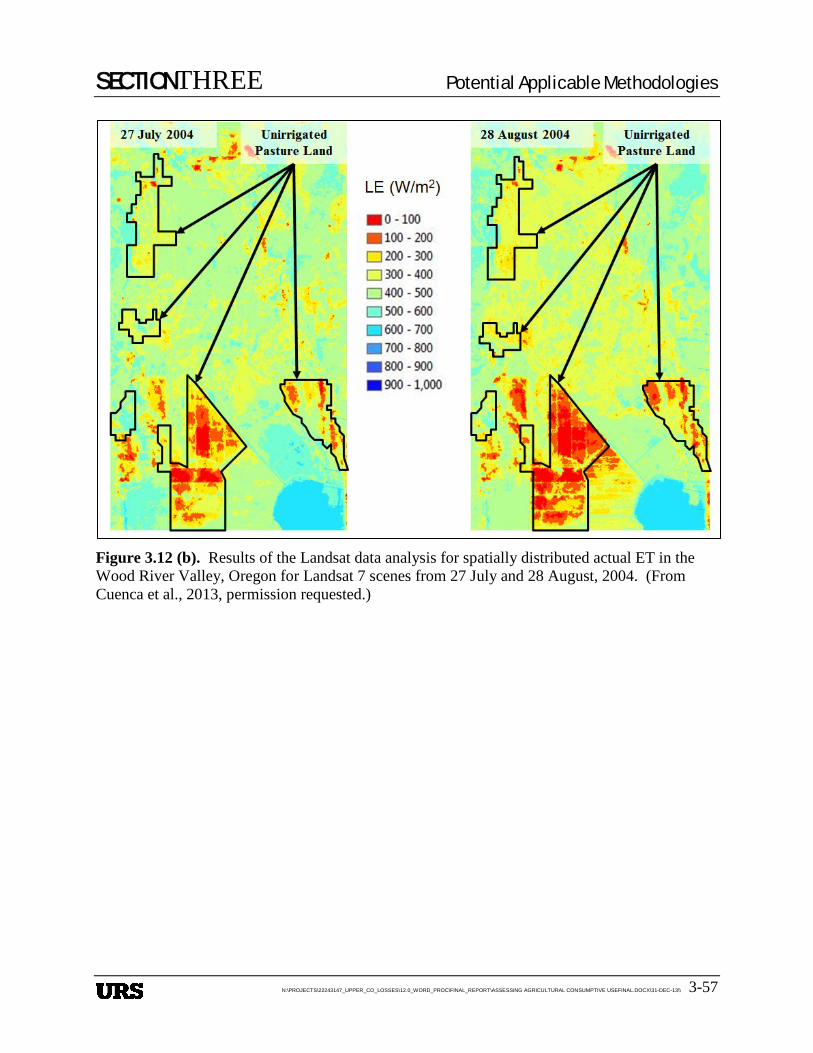
SECTIONTHREE Potential Applicable Methodologies
N:\PROJECTS\22243147_UPPER_CO_LOSSES\12.0_WORD_PROC\FINAL_REPORT\ASSESSING AGRICULTURAL CONSUMPTIVE USEFINAL.DOCX\31-DEC-13\\ 3-57
Figure 3.12 (b). Results of the Landsat data analysis for spatially distributed actual ET in the Wood River Valley, Oregon for Landsat 7 scenes from 27 July and 28 August, 2004. (From Cuenca et al., 2013, permission requested.)
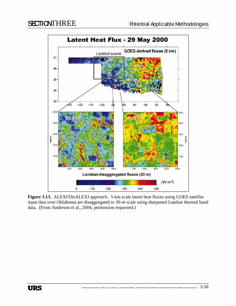
SECTIONTHREE Potential Applicable Methodologies
N:\PROJECTS\22243147_UPPER_CO_LOSSES\12.0_WORD_PROC\FINAL_REPORT\ASSESSING AGRICULTURAL CONSUMPTIVE USEFINAL.DOCX\31-DEC-13\\ 3-58
Figure 3.13. ALEXI/DisALEXI approach. 5-km scale latent heat fluxes using GOES satellite input data over Oklahoma are disaggregated to 30-m scale using sharpened Landsat thermal band data. (From Anderson et al., 2004, permission requested.)
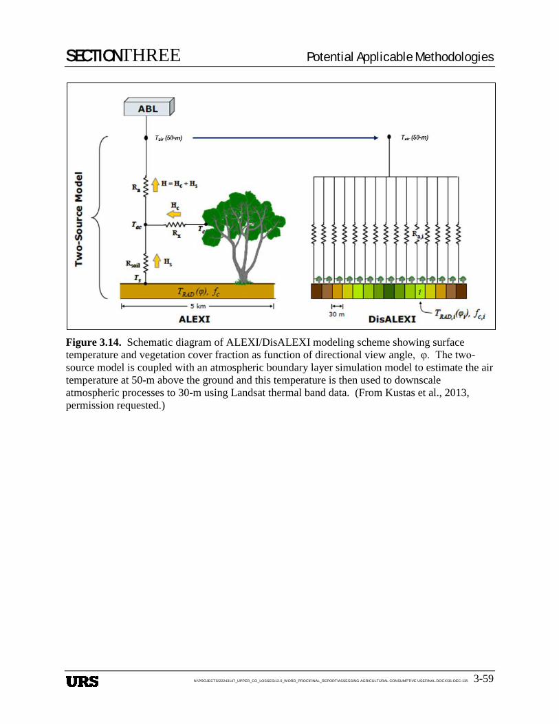
SECTIONTHREE Potential Applicable Methodologies
N:\PROJECTS\22243147_UPPER_CO_LOSSES\12.0_WORD_PROC\FINAL_REPORT\ASSESSING AGRICULTURAL CONSUMPTIVE USEFINAL.DOCX\31-DEC-13\\ 3-59
Figure 3.14. Schematic diagram of ALEXI/DisALEXI modeling scheme showing surface temperature and vegetation cover fraction as function of directional view angle, φ. The two-source model is coupled with an atmospheric boundary layer simulation model to estimate the air temperature at 50-m above the ground and this temperature is then used to downscale atmospheric processes to 30-m using Landsat thermal band data. (From Kustas et al., 2013, permission requested.)
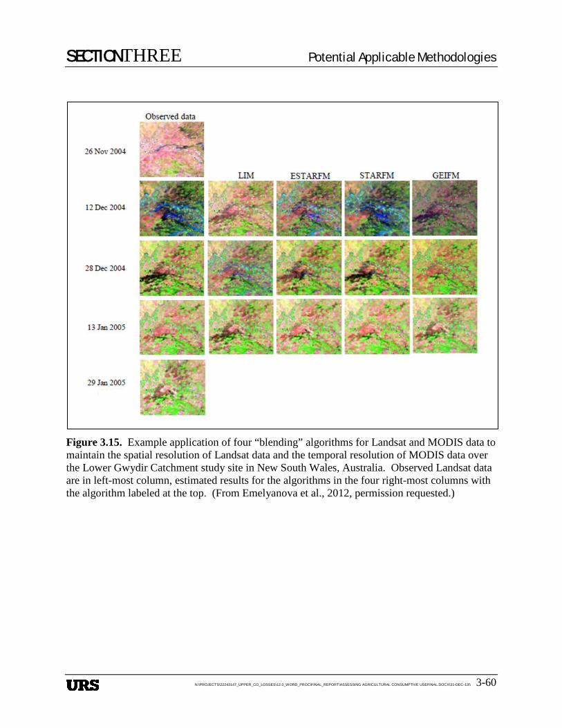
SECTIONTHREE Potential Applicable Methodologies
N:\PROJECTS\22243147_UPPER_CO_LOSSES\12.0_WORD_PROC\FINAL_REPORT\ASSESSING AGRICULTURAL CONSUMPTIVE USEFINAL.DOCX\31-DEC-13\\ 3-60
Figure 3.15. Example application of four “blending” algorithms for Landsat and MODIS data to maintain the spatial resolution of Landsat data and the temporal resolution of MODIS data over the Lower Gwydir Catchment study site in New South Wales, Australia. Observed Landsat data are in left-most column, estimated results for the algorithms in the four right-most columns with the algorithm labeled at the top. (From Emelyanova et al., 2012, permission requested.)

SECTIONTHREE Potential Applicable Methodologies
N:\PROJECTS\22243147_UPPER_CO_LOSSES\12.0_WORD_PROC\FINAL_REPORT\ASSESSING AGRICULTURAL CONSUMPTIVE USEFINAL.DOCX\31-DEC-13\\ 3-61
Figure 3.16. Example application of ALEXI-DisALEXI downscaling together with the STARFM interpolating algorithm for daily evapotranspiration over nine days near Orlando, FL in 2002. This study required application of GOES, MODIS and Landsat data. (From Anderson et al., 2013, with permission).
Figure 3.17. Left: Close up of reference ET fraction, ETrF, image from an area near Christmas Valley, Oregon on 17 June 2004. Right: The same ETrF map but calculated using “sharpened” surface temperature based on NDVI distribution. (From Allen, 2012, with permission.)
SECTIONFOUR References
N:\PROJECTS\22243147_UPPER_CO_LOSSES\12.0_WORD_PROC\FINAL_REPORT\ASSESSING AGRICULTURAL CONSUMPTIVE USEFINAL.DOCX\31-DEC-13\\ 4-1
4. Section 4 FOUR References
REFERENCES 4.1Abrahamsen, P. and S. Hansen. 2000. Daisy: an open soil-crop-atmosphere model.
Environmental Modelling & Software, Vol. 15: pp. 313–330.
Agam, N., W. P. Kustas, M. C. Anderson, F. Li and C. M. U. Neale. 2007. A vegetation index based technique for spatial sharpening of thermal imagery. Remote Sensing of Environment. Vol. 107, pp. 545-558.
Allen, R.G., L. Pereira, D. Rase, and M. Smith. 1998. Crop Evapotranspiration, Irrigation and Drainage Paper 56. Food and Agriculture Organization of the United Nations, Rome, Italy. ISBN 92-5-104219-5. 300 pp.
Allen, R.G.; Tasumi, M.; Trezza, R.; Waters, R. 2002. Mapping Evapotranspiration at High Resolution and using Internalized Calibration. Advanced Training and User’s Manual, Ver. 1.0. 99 pp.
Allen, R. G., I. A. Walter, R. Elliot, T. A. Howell, D. Itenfisu, M. Jensen (editors), R. H. Cuenca, J. L. Wright, P. Brown, B. Mecham, R. Snyder, S. Eching, T. Spofford, M. Hattendorf and D. Martin. 2005. The ASCE Standardized Reference Evapotranspiration Equation, American Society of Civil Engineers, 216 pp.
Allen, R.G., M. Tasumi, A. Morse, R. Trezza, J.L Wright, W.G.M. Bastiaanssen, W. Kramber, I. Lorite and C.W. Robison. 2007. Satellite-based energy balance for mapping evapotranspiration with internalized calibration (METRIC) — Applications. ASCE Journal of Irrigation and Drainage Engineering. Vol. 133, pp. 395–406.
Allen, R.G.; Tasumi, M.; Morse, A.T.; Trezza, R. A. 2005. Landsat-based energy balance and evapotranspiration model in western U.S. water rights regulation and planning. Journal of Irrigation and Drainage Systems. Vol. 19, pp. 251–268.
Allen, R.G. 2000. REF-ET: Reference Evapotranspiration Calculation Software for FAO and ASCE Standardized Equations. University of Idaho.
Allen, R.G., M. Tasumi and R. Trezza. 2007. Satellite-based energy balance for mapping evapotranspiration with internalized calibration (METRIC) – Model. ASCE Journal of Irrigation and Drainage Engineering. Vol. 133(4), pp. 380-394.
Allen, R.G., Tasumi, M., Trezza, R., Kjaersgaard, J.H., 2010. METRIC. Mapping Evapotranspiration at High Resolution. Applications Manual, V 2.0.4. University of Idaho. 166 pp.
Allen, R.G. 2012. Training material for METRIC course at Reno, NV, personal communication.
Allen, R,G. 2012. Field Scale Estimation of Evapotranspiration for Water Rights Management. Presentation at Western States Remote Sensing Workshop. Boise, ID.
Allen, Richard G., Boyd Burnett, William Kramber, Justin Huntington, Jeppe Kjaersgaard, Ayse Kilic, Carlos Kelly, and Ricardo Trezza, 2013. Automated Calibration of the METRIC-Landsat Evapotranspiration Process. Journal of the American Water Resources Association (JAWRA) 49(3): 563-576. DOI: 10.1111/jawr.12056.
SECTIONFOUR References
N:\PROJECTS\22243147_UPPER_CO_LOSSES\12.0_WORD_PROC\FINAL_REPORT\ASSESSING AGRICULTURAL CONSUMPTIVE USEFINAL.DOCX\31-DEC-13\\ 4-2
Anderson, M. C., J. M. Norman, J. R. Mecikalski, R. D. Torn, W. P. Kustas and J. B. Basara. 2004. A multi-scale remote sensing model for disaggregating regional fluxes to micrometeorological scales. Journal of Hydrometeorology. Vol. 5, pp. 343-363.
Anderson, M.C., W.P. Kustas, J.M. Norman, C.R. Hain, J.R. Mecikalski, L. Schultz, M.P. Gonzalez-Dugo, C. Cammalleri, G. d'Urso, A. Pimstein and F. Gao. 2011. Mapping daily evapotranspiration at field to continental scales using geostationary and polar orbiting satellite imagery. Hydrology and Earth System Sciences, 15(1), pp. 223-239.
Bastiaanssen, W.G.M., Menenti, M.; Feddes, R.A.; Holtslag, A.A.M. 1998. A remote sensing surface energy balance algorithm for land (SEBAL); 1. formulation. Journal of Hydrology. Vol. 212–213, pp. 198–212.
Bastiaanssen, W.G.M. 2000. SEBAL based sensible and latent heat fluxes in the irrigated Gediz Basin, Turkey. Journal of Hydrology. Vol. 229, pp. 87–100.
Bastiaanssen, W. G. M., Noordman, E. J. M., Pelgrum, H., Davids, G., Thoreson, B. P., and Allen, R. G. _2005_. “SEBAL model with remotely sensed data to improve water-resources management under actual field conditions.” J. Irrig. Drain. Eng., Vol. 131, No.1, pp. 85–93.
Beamer, J. P.; Huntington, J. L.; Morton, C. G.; Pohll, G. M. 2013. Estimating Annual Groundwater Evapotranspiration from Phreatophytes in the Great Basin using Landsat and Flux Tower Measurements Journal of the American Water Resources Association (JAWRA).49(3):518–533 Bowen, I. S. 1926. The ratio of heat losses by conduction and by evaporation from any water surface. Physics Review. Vol. 27, pp. 779 – 787.
Brotzge, J. A., S. Richardson, K. Crawford, T. Horst, F. Brock, K. Humes, Z. Sorbjan and R. Elliott. 1999. The Oklahoma Atmospheric Surface-layer Instrumentation System (OASIS) Project. Preprints, 13th Symposium on Boundary Layers and Turbulence, Dallas, TX, American Meteorological Society, pp. 612–615.
Brunt, D. Notes on Radiation in the Atmosphere I (1932) Quarterly Journal of the Royal Meteorological Society Volume 58, Issue 247, pages 389–420, October 1932
Choudhury, B. J., N. U. Ahmed, S. B. Idso, R. J. Reginato and C. S. T. Daughtry. 1994. Relations between evaporation coefficients and vegetation indices studied by model simulations. Remote Sensing of Environment, 50, pp. 1–17.
Cuenca, R. H. 1989. Irrigation System Design - An Engineering Approach. Prentice-Hall, Inc., Englewood Cliffs, NJ. 552 pp.
Cuenca, R.H., S.P. Ciotti and Y. Hagimoto. 2013. Application of Landsat to Evaluate effects of Irrigation Forbearance. Remote Sensing. 5, pp. 3776-3802; doi:10.3390/rs5083776.
Diak, G. R., W. L. Bland and J. R. Mecikalski. 1996. A note on first estimates of surface insolation from GOES-8 visible satellite data. Agricultural and Forest Meteorology, 82, pp. 219–226.
Diak, G. R., W. L. Bland, J. R. Mecikalski and M.C. Anderson. 2000. Satellite-based estimates of longwave radiation for agricultural applications. Agricultural and Forest Meteorology, 103, pp. 349–355.
SECTIONFOUR References
N:\PROJECTS\22243147_UPPER_CO_LOSSES\12.0_WORD_PROC\FINAL_REPORT\ASSESSING AGRICULTURAL CONSUMPTIVE USEFINAL.DOCX\31-DEC-13\\ 4-3
Eckhardt, D. 2013. Mapping Evapotranspiration in the Upper Colorado River Basin using the ReSET Energy-Balance Model. Technical Memorandum 86-68260-13-01, Bureau of Reclamation. (Draft)
Eidenshink, J. C. 1992. The 1990 conterminous U.S. AVHRR data set. Photogrammetric Engineering and Remote Sensing, 58, pp. 809–813.
Emelyanova IV, McVicar TR, Van Niel TG, Li LT, van Dijk AIJM. 2012. On blending Landsat-MODIS surface reflectances in two landscapes with contrasting spectral, spatial and temporal dynamics. WIRADA Project 3.4 : Technical report. CSIRO Water for a Healthy Country Flagship, Australia. 72 pp.
French, A.N., F. Jacob, M.C. Anderson, W.P. Kustas, W. Timmermans, A. Gieske, Z. Su, H. Su, M.F. McCabe, F. Li, J. Prueger and N. Brunsell. 2005. Surface energy fluxes with the Advanced Spaceborne Thermal Emission and Reflection radiometer (ASTER) at the Iowa 2002 SMACEX site (USA). Remote Sensing of Environment, Vol. 99, pp. 55-65.
French, A. N., J. M. Norman and M. C. Anderson. 2003. Simplified correction of GOES thermal infrared observations. Remote Sensing of Environment, 87, pp. 326–333.
Gao F, Masek J, Schwaller M and Hall F. 2006. On the blending of the Landsat and MODIS surface reflectance: predicting daily Landsat surface reflectance. IEEE Transactions on Geoscience and Remote Sensing, 44(8), pp. 2207-2218.
Irmak, A., I. Ratcliff, P. Ranade, K. Hubbard, R.K. Singh, B. Kamble and J. Kjaersgaard. 2011. Estimation of Land Surface Evapotranspiration with a Satellite Remote Sensing Procedure. Great Plains Research, No. 21 (Spring 2011): pp. 73-88, Univ. of Nebraska-Lincoln.
Irmak, A., R.G. Allen, J.L. Kjaersgaard, J. Huntington, B. Kamble, R. Trezza, I. Ratcliffe. 2012. Operational Remote Sensing of ET and Challenges. Evapotranspiration: Remote Sensing and Modeling. InTech. ISBN:978-953-307-808-3.
Irons, J. R.; Dwyer, J.L.; Barsi, J.A. 2012. The next Landsat satellite: The Landsat Data Continuity Mission. Remote Sensing of the Environment. Vol. 122: pp. 11-21.
Jensen, M.E., R.D. Burman, R.G. Allen (editors), R.H. Cuenca (contributing author), and others. 1990. Evapotranspiration and Irrigation Water Requirements. ASCE Engineering Practices Manual No. 70, Committee on Irrigation Water Requirements, American Society of Civil Engineers. 332 pp.
Kalma, J. D., T.R. McVicar and M.F. McCabe. 2008. Estimating land surface evaporation: A review of methods using remotely sensed surface temperature data. Surveys in Geophysics. Vol. 29. pp. 421-469.
Kjaersgaard, J.; Allen, R.; Irmak, A. 2011. Improved methods for estimating monthly and growing season ET using METRIC applied to moderate resolution satellite imagery. Hydrological Processes. Vol. 25, pp. 4028-4036.
Kjaersgaard, J., B. Hankerson and C. Hay. 2012. ASA International Annual Meeting, Climatology & Modeling, 23 October 2012. Cincinnati, Ohio.
Kleissl, J., J. Gomez, S-H. Hong, J. Hendrickx, T. Rahn and W. Defoor. 2008. Large aperture scintillometer intercomparison study. Boundary-Layer Meteorology, Vol. 128, pp. 133-150.
SECTIONFOUR References
N:\PROJECTS\22243147_UPPER_CO_LOSSES\12.0_WORD_PROC\FINAL_REPORT\ASSESSING AGRICULTURAL CONSUMPTIVE USEFINAL.DOCX\31-DEC-13\\ 4-4
Kleissl, J, C.J. Watts, J.C. Rodriguez, S. Naif and E.R. Vivoni. 2009. Scintillometer intercomparison study - Continued. Boundary-Layer Meteorology, Vol. 130, pp. 437-443.
Kustas, W.P. and J. D. Albertson. 2003. Effects of surface temperature contrast on land–atmosphere exchange: A case study from Monsoon 90. Water Resources Research, 39, 1159, doi:10.1029/2001WR001226.
Kustas, W. P., J. M. Norman, M. C. Anderson and A. N. French. 2003. Estimating subpixel surface temperature and energy fluxes from the vegetation index-radiometric temperature relationship. Remote Sensing of Environment. Vol. 85, pp. 429-440.
Kustas, W.P., J.L. Hatfield and J.H. Prueger. 2005. The soil moisture-atmosphere coupling experiments (SMACEX): Background, hydrometeorological conditions, and preliminary findings. Journal of Hydrometeorology, 6, pp. 791–804.
Long, D. and V.P. Singh. 2013. Assessing the impact of end-member selection on the accuracy of satellite-based spatial variability models for actual evapotranspiration estimation. Water Resources Research, 49, pp. 2601–2618.
Mahrt, L. (2000). Surface heterogeneity and vertical structure of the boundary layer. Boundary-Layer Meteorology, Vol. 96, pp. 33– 62.
Maurer, D.K., D.L. Berger, M.L. Tumbusch, and M.J. Johnson. 2006. Rates of Evapotranspiration, Recharge from Precipitation Beneath Selected Areas of Native Vegetation, and Streamflow Gain and Loss in Carson Valley, Douglas County, Nevada, and Alpine County, California; US Geological Survey Scientific Investigations Report 2005-5288; USGS: Reston, VA, USA. Available online: http://pubs.usgs.gov/sir/2005/5288/ (accessed on 30 July 2013).
McNaughton, K. G. and T. W. Spriggs. 1986. A mixed-layer model for regional evaporation. Boundary-Layer Meteorology, 74, pp. 262–288.
Mecikalski, J. M., G. R. Diak, M. C. Anderson and J. M. Norman. 1999. Estimating fluxes on continental scales using remotely sensed data in an atmosphere–land exchange model. Journal of Applied Meteorology, 38, pp. 1352–1369.
Melton, F.S., L.F. Johnson, C.P. Lund, L.L. Pierce, A.R. Michaelis, S.H. Hiatt, A. Guzman, D.D. Adhikari, A.J. Purdy, C. Rosevelt, P. Votava, T.J. Trout, B. Temesgen, K. Frame. E.J. Sheffner and R. R. Nemani. 2012. Satellite Irrigation Management Support with the Terrestrial Observation and Prediction System: A framework for integration and surface observations to support improvements in agricultural Water Resource management. IEEE Journal of Selected Topics in Applied Earth Observations and Remote Sensing. Vol. 5, pp. 1709-1721.
Morton, C.G., J.L. Huntington, G.M. Pohll, R.G. Allen, K.C. McGwire and S.D. Bassett. 2013. Assessing calibration uncertainty and automation for estimating evapotranspiration from agricultural areas using METRIC. Journal of the American Water Resources Association (JAWRA).49(3):549–562 Nagler, P. L.; Scott, R. L.; Westenburg, C.; Cleverly, J. I.; Glenn, E.P.; Huete, A. H. 2005. Evapotranspiration on Western U.S. Rivers Estimated Using the Enhanced Vegetation Index from MODIS and Data from Eddy Covariance and Bowen Ratio Flux Towers. Remote Sensing of the Environment. Vol. 97, pp. 337-351.
SECTIONFOUR References
N:\PROJECTS\22243147_UPPER_CO_LOSSES\12.0_WORD_PROC\FINAL_REPORT\ASSESSING AGRICULTURAL CONSUMPTIVE USEFINAL.DOCX\31-DEC-13\\ 4-5
Nash, L. E. and J. V. Sutcliffe. 1970. River flow forecasting through conceptual models—Part 1: A discussion of principles. Journal of Hydrology, 10, pp. 282–290.
Nichols, W. E. and R. H. Cuenca. 1993. The Evaporative Fraction as a Measure of Surface Energy Partitioning. Water Resources Research, Vol. 29 (11), pp. 3681 - 3690.
Norman, J.M., M.C. Anderson, W.P. Kustas, A.N. French, J. Mecikalski, R. Torn, G.R. Diak, T. J. Schmugge and B.C.W. Tanner. 2003. Remote sensing of surface energy fluxes at 101-m pixel resolutions. Water Resources Research, 39, 1221, doi: 10.1029/2002WR001775.
Paulson, C.A. 1970. The mathematical representation of wind speed and temperature profiles in the unstable atmospheric surface layer. Applied Meteorology. Vol. 9, pp. 857-861.
Priestley, C. H. B. and R. J. Taylor. 1972. On the assessment of surface heat flux and evaporation using large-scale parameters. Monthly Weather Review, 100, pp. 81–92.
Schuepp, P. H., M. Y. Leclerc, J. I. MacPherson and R. L. Desjardins. 1990. Footprint prediction of scalar fluxes from analytical solutions of the diffusion equation. Boundary-Layer Meteorology, 50, pp. 355–373.
Schuepp, P. H., J. I. MacPherson and R. L. Desjardins. 1992. Adjustment of footprint correction for airborne flux mapping over the FIFE site. Journal of Geophysical Research, 97, 18 455–18 466.
Shuttleworth, W. J., R. J. Gurney, A. Y. Hsu, and J.P. Ormsby. 1989. FIFE: The variation in energy partition at surface flux sites, in Remote Sensing and Large-Scale Global Processes (Proceedings of the IAHS Third International Assembly, Baltimore, MD, May 1989), edited by A. Rango, IAHS Publ., 186, 67-74.
Tasumi, M. 2003. Progress in operational estimation of regional evapotranspiration using satellite imagery. Dissertation, 357 Idaho: University of Idaho.
Tasumi, M.; Allen, R.G.; Trezza, R. 2008. At-surface reflectance and albedo from satellite for operational calculation of land surface energy balance. ASCE Journal of Hydrologic Engineering. Vol. 13, pp. 51-63.
Timmermans, W.J., W.P. Kustas, M.C. Anderson and A.N. French. 2007. An intercomparison of the surface energy balance algorithm for land (SEBAL) and the two-source energy balance (TSEB) modeling schemes. Remote Sensing of Environment, 108, pp. 369–384.
Ungar, S.G.; Pearlman, J. S.; Mendenhall, J. A.; Reuter, D. 2003. Overview of the Earth Observing One (EO-1) mission. IEEE T Geosci Remote. Vol. 41, pp. 1149–1159.
Webb, E.K. 1970. Profile relationships: the log-linear range, and extension to strong stability. Quarterly Journal of the Royal Meteorological Society. Vol. 96, pp. 67-90.
Wilson K, E. Falge, M. Aubinet, D. Baldocchi, A. Goldstein and P. Berbigier. 2002. Energy balance closure at FLUXNET sites. Agricultural and Forest Meteorology. Vol. 113, pp. 223–243. doi:10.1016/S0168-1923(02)00109-0

Appendix A Colorado
Appendix A Colorado
A-1
Introduction This appendix documents the methods, models and available information that Colorado is currently using to estimate water supply-limited crop consumptive use (irrigation CU) for irrigated lands in the Upper Colorado River basin, and other areas of the State. This appendix provides information that supports the overall project goal of developing a coordinated long-term process among the Upper Division States (Colorado, New Mexico, Utah, and Wyoming) to estimate irrigation CU for irrigated lands in the entire Upper Colorado River basin.
Members of the URS Team have been involved with estimating crop consumptive use in Colorado for various purposes, including developing Colorado’s portion of the Consumptive Uses and Losses Report for the Colorado Water Conservation Board. The URS Team is familiar with the consumptive use methods, available information, and modeling software/programs that Colorado is currently using in the Upper Colorado River basin. This appendix was reviewed by Colorado Division of Water Resources staff as to general approach and methodologies.
Irrigated Acreage Assessment Availability and Attribution Irrigated acreage assessments define the amount of acreage that was actively irrigated and cultivated in any given year. Irrigated acreage assessments can range in the level of attribution; detailed assessments can include the attribution of:
• Crop Types • Supply Type, such as surface water, ground water, reservoir releases, or multiple sources • Supply Source, including name or unique identifier of the water permit or water right,
diversion structure, well, or reservoir • Irrigation Method, such as flood or sprinkler irrigation practices
The following describes the assessment efforts for Colorado for irrigated acreage in the Western Slope river basins (White, Yampa, San Juan, Upper Colorado and Gunnison River basins); including the availability of historical assessments, spatial format of assessments, availability of attributes, and expected assessment efforts in the future.
Irrigated acreage was first developed in a GIS platform in Colorado in the mid-1990s by the U.S. Bureau of Reclamation (Reclamation) in support of the Colorado River System Consumptive Use and Losses Report (CU and Losses). The GIS assessment identified irrigated parcels based on 1993 aerial imagery and attributed the acreage with crop types based on County Agricultural Statistics. With assistance from the State Engineer’s Office, the 1993 irrigated acreage shapefile was also attributed with supply type(s), supply source(s) and irrigation method. Subsequent acreage assessments for the Western Slope were completed by the State to delineate and attribute irrigated acreage in 2000 and 2005, and the State is currently working on a 2010 acreage assessment. Delineation of irrigated parcels is based on satellite imagery and aerial photography, with some on the ground review by water commissioners. There are concerns with the accuracy of the 2000 acreage assessment, and it is generally not used by the State for planning or administrative purposes. The 2005 acreage assessment however is considered generally representative of the irrigated acreage conditions. The State is currently performing a review of the 2005 assessment with the Division staff in each basin to refine the supply source attribution to improve the overall accuracy of that assessment. The 2010 acreage assessment is

Appendix A Colorado
A-2
currently underway, and it is anticipated that this coverage will be refined based on the results of the 2005 source attribution review efforts. Table 1 summarizes the total acreage by Division from the 1993, 2005, and 2010 assessments. Note that based on the review currently underway, these numbers may change slightly. One of the issues being investigated is how/if acreage is considered under ditch systems that continue to irrigate parcels within municipal boundaries. This issue is especially important in the growing urban area around Grand Junction.
Table 1: 1993, 2005, and 2010 Irrigated Acreage
River Basin Total 1993 Irrigated Acreage
Total 2005 Irrigated Acreage
Total 2010 Irrigated Acreage
Gunnison 310,235 286,254 N/A
Upper Colorado 270,883 226,375 196,831
White 26,577 27,517 N/A
Yampa 93,093 74,528 N/A
San Juan 210,888 176,453 N/A
Total 911,676 791,127 N/A
Much of the irrigated acreage in the high elevations of the Western Slope river basins is flood-irrigated hay meadows and various high-elevation grass mixtures. In the lower elevations, there is more variety of crops; including alfalfa, orchards, corn, small grains, and vegetables near the Grand Junction and Delta area, and alfalfa near the Cortez area. Previous estimates of crop type were based on County Agricultural Statistic data, concentrating only on areas of lower elevation. For 2010, the State began using the grid-based National Agricultural Statistics Service Cropland Data Layer (NASS CDL) data to assign crop types to the lower elevations. There has been a small decrease in irrigated acreage and crops grown in the Western Slope river basins due to urban or other development. In order to capture these changes, the State’s goal is to develop acreage assessments on an approximately 5-year basis. At this time, the State is refining the assignment of water source attributes in historical assessments; planning on the incorporation of the 2005 and 2010 acreage assessments in future CU and Losses and Colorado’s Decision Support Systems (CDSS) planning efforts; and planning to develop a 2015 acreage assessment to capture changes to acreage in the future. The GIS assessments are available on the CDSS website (http://cdss.state.co.us). Additionally, the attribute information is stored in HydroBase, a central database that houses real-time, historical and geographic water resources related data in Colorado. HydroBase data can be accessed either through the CDSS website, or through data management interfaces that query and format data. Summary In most areas of irrigation in the Western Slope basins, acreage and crop types have been relatively consistent for the past 50 plus years. The 5-year irrigated acreage assessments are sufficient to represent changes in irrigated acreage and crop type for these areas. There are a few
Appendix A Colorado
A-3
areas of more productive irrigation in the lower elevation, for example the Uncompahgre Valley, Grand Valley, and Dolores Project areas. These areas are more likely to experience changes in crop types, and potentially changes in acreage due to urbanization. It may be important to estimate crop types in these areas more frequently than every five years; however, the slow decreases in irrigated parcels in these areas can be captured with 5-year assessments.
Climate Data Availability Climate data serves as the basis for estimating the amount of water needed by a crop; climate data availability can be assessed in terms of:
• Spatial Distribution - is there a sufficient distribution of climate stations in proximity to irrigated acreage in the basin to accurately measure the climatic conditions experienced by the acreage?
• Climate Data Measured - what types of climatic factors (e.g. precipitation, wind speed, solar radiation) are recorded at each station?
Understanding the distribution and types of climate data in each basin is important because different consumptive use methods require different climate data information; and significant distance between the irrigated acreage and the climate station produces less accurate consumptive use estimates.
For purposes of this study, climate stations are categorized based on the types of data measured. Stations recording temperature and precipitation only are termed “Temperature/Precipitation” stations. Stations that record temperature and precipitation plus relative humidity, sky/cloud cover, solar radiation, wind speed and direction, and barometric pressure readings are termed “Extended Climate” stations. The following describes the climate stations in the Western Slope river basins (White, Yampa, San Juan, Upper Colorado and Gunnison River basins) and discusses their general data availability and proximity to irrigated lands.
Climate data from a majority of the Extended Climate stations located in the Western Slope river basins are available through the Colorado Agricultural Meteorological Network (CoAgMet), managed by the Colorado Climate Center (CCC) at Colorado State University. Data from these climate stations, generally located in agricultural areas, is available both in HydroBase and online from the CoAgMet website, generally beginning in the early 1990’s. Table 2 lists the currently active CoAgMet stations and their associated elevation and first observation dates.
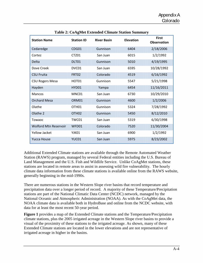
Appendix A Colorado
A-4
Table 2: CoAgMet Extended Climate Station Summary
Station Name Station ID River Basin Elevation First Observation
Cedaredge CDG01 Gunnison 6404 2/18/2006
Cortez CTZ01 San Juan 6015 1/2/1992
Delta DLT01 Gunnison 5010 4/19/1995
Dove Creek DVC01 San Juan 6595 10/28/1992
CSU Fruita FRT02 Colorado 4519 6/16/1992
CSU Rogers Mesa HOT01 Gunnison 5547 5/21/1998
Hayden HYD01 Yampa 6454 11/16/2011
Mancos MNC01 San Juan 6730 10/29/2010
Orchard Mesa ORM01 Gunnison 4600 1/2/2006
Olathe OTH01 Gunnison 5324 7/28/1992
Olathe 2 OTH02 Gunnison 5450 8/12/2010
Towaoc TWC01 San Juan 5319 6/30/1998
Wolford Mtn Reservoir WFD01 Colorado 7520 11/30/2004
Yellow Jacket YJK01 San Juan 6900 1/2/1992
Yucca House YUC01 San Juan 5975 8/23/2002
Additional Extended Climate stations are available through the Remote Automated Weather Station (RAWS) program, managed by several Federal entities including the U.S. Bureau of Land Management and the U.S. Fish and Wildlife Service. Unlike CoAgMet stations, these stations are located in remote areas to assist in assessing wild fire vulnerability. The hourly climate data information from these climate stations is available online from the RAWS website, generally beginning in the mid-1990s. There are numerous stations in the Western Slope river basins that record temperature and precipitation data over a longer period of record. A majority of these Temperature/Precipitation stations are part of the National Climatic Data Center (NCDC) network, managed by the National Oceanic and Atmospheric Administration (NOAA). As with the CoAgMet data, the NOAA climate data is available both in HydroBase and online from the NCDC website, with data for at least the most recent 50-year period. Figure 1 provides a map of the Extended Climate stations and the Temperature/Precipitation climate stations, plus the 2005 irrigated acreage in the Western Slope river basins to provide a visual of the proximity of these stations to the irrigated acreage. As shown, many of these Extended Climate stations are located in the lower elevations and are not representative of irrigated acreage in higher in the basins.
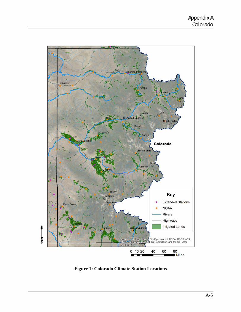
Appendix A Colorado
A-5
Figure 1: Colorado Climate Station Locations
Appendix A Colorado
A-6
Additional Temperature/Precipitation climate stations are available through the Snotel network of stations managed by the National Resources Conservation Service (NRCS), and through the Community Collaborative Rain, Hail and Snow (CoCoRaHS) network managed by the CCC. As the primary purpose of Snotel and CoCoRaHS networks are to measure snow and precipitation data, many of these stations are located in higher elevations. Climate data, along with maps and summary reports from these climate stations, are available online from their respective websites (http://www.wcc.nrcs.usda.gov/snow/, http://ccc.atmos.colostate.edu/).
In addition to tabular climate data, the available format for the climate stations discussed above, climate information can also be processed and distributed in a grid format. There are programs that provide grid-based climate data for the entire Colorado River Basin, including the Western Slope river basins. Temperature/Precipitation climate grids are available through the PRISM (Parameter-elevation Regressions on Independent Slopes Model) Climate Group program. Gridded extended climate data is available through the North America Land Data Assimilation System (NLDAS).
Summary The spatial distribution of the temperature/precipitation and extended climate data stations provide good coverage of the basin, with increased density of stations near irrigated lands in areas under about 6500 feet elevation. The CoAgMet stations and most of the NOAA stations are located within irrigated fields. Although the RAWS stations are generally not in agricultural areas, they do provide climate data at higher elevations better representing high meadows in Colorado. The number and density of Extended Climate stations appears to be sufficient to determine crop consumptive use using the more data-intensive daily consumptive use methods and to support calibration and verification of remote sensing methods below 6500 feet elevation.
Quality review and correction of daily Extended Climate station data is recommended prior to use and standard procedures have been developed and documented in ASCE Standardized Reference Evaporation Equation Handbook. Although standardized, this quality review can be time-consuming and requires more effort than using monthly temperature and precipitation data, which is reviewed prior to publication and does not require additional quality control.
Potential Crop Consumptive Use Methods There are many different methodologies that estimate PCU, or the amount of water that would be used for crop growth if provided with an ample water supply. They range in complexity, accuracy and data requirements. This section describes methods used in the Western Slope river basins for CU and Losses reporting as well as other planning efforts.
The State of Colorado has historically used the SCS TR-21 Modified and Original Blaney-Criddle methods to estimate PCU for their internal CU and Losses reporting of crop consumptive use. The Blaney-Criddle methodologies consist of an empirical equation that relates evapotranspiration with mean air temperature and mean percentage daylight hours. The SCS TR-21 method was modified from the Original Blaney-Criddle method to reasonably estimate seasonal consumptive use. The modifications include the use of (1) climatic coefficients that are directly related to the mean air temperature for each of the consecutive short periods which constitutes the growing season and (2) coefficients which reflect the influence of the crop growth rates on consumptive use rates. The modified Blaney-Criddle crop coefficients are available
Appendix A Colorado
A-7
from graphs in the SCS TR-21 publication for 25 crops, which were developed based on general climatic conditions representative of the Western U.S.
The ASCE Manual No. 70 recommends an elevation adjustment of 10 percent increase in PCU for each 1,000 meters increase in elevation above sea level for the SCS Modified Blaney-Criddle method when using standard TR-21 crop coefficients. The adjustment corrects for lower mean temperatures that occur at higher elevations at a given level of solar radiation (i.e. mean temperatures do not reflect crops’ reactions to warm daytime temperatures and cool nights). The recommended adjustment is applied to the PCU estimate and to all crop types. The State of Colorado uses SCS TR-21 coefficients with this standard elevation adjustment in the Western Slope river basins below about 6500 feet elevation when estimating basin-wide PCU for their internal CU and Losses reporting.
Above 6500 feet in the Western Slope river basins, the Original Blaney-Criddle method is used with locally calibrated coefficients to represent local climatic conditions. The calibrated coefficients, referred to as the Denver Water High Altitude coefficients, were summarized in a report prepared for Denver Water that compared lysimeter results from South Park, Colorado to estimated PCU using the calibrated coefficients in the Original Blaney-Criddle method. Note that as the coefficients were calibrated to high altitude lysimeters, an additional elevation adjustment is not appropriate and has not been applied. PCU estimates with these calibrated coefficients have compared well with estimates from lysimeter studies in other high-elevation areas of Colorado, including near the town of Gunnison. The Denver Water High Altitude crop coefficients have been used on a basin-wide scale to estimate PCU for grass pasture crops above 6,500 feet in elevation with the Original Blaney-Criddle methodology in the Western Slope river basins.
The SCS Blaney-Criddle method has been used to estimate PCU in other river basins under Colorado’s Decision Support Systems, which are used for various administrative and operational planning efforts by the State. TR-21 Blaney-Criddle crop coefficients have been calibrated to local conditions in other basins based on lysimeter data and/or more detailed daily PCU methods (modified daily Hargreaves and ASCE Standardized Penman).
The SCS Blaney-Criddle monthly methodology is preferred by the State for historical consumptive use estimates because the climate data required is available over a very long period that corresponds with available diversion data and reflects varying hydrology and climatic conditions. This preference is also seen in Colorado’s Water Courts where it is necessary to prove consumptive use over a longer period and Extended Climate data required for more data-intensive methodologies is not available. The difference in accuracy between the simpler Blaney-Criddle methods requiring only temperature climate data and more data-intensive methods is documented in ASCE Manual 70; and the use of high-altitude adjustments and locally calibrated coefficients is a reasonable approach to allow the simpler methods to be more accurately used for longer historical assessments.
Additional daily methodologies are used on a smaller scale within the State; for example, to develop calibrated crop coefficients for monthly methods, compare the accuracy of different methods, apply the results to irrigation efficiencies or scheduling, or perform field-level analyses. These methodologies include:
• ASCE Standardized Penman-Monteith. This method, which is a slight simplification of the Penman-Monteith equation, consisting of two reference evapotranspiration (ET)
Appendix A Colorado
A-8
equations, one for a short crop and one for a taller crop. Reference ET equations require daily temperature, solar radiation, vapor pressure and wind speed data. The coefficients for both short and taller crops are provided in ASCE Manual 70.
• Hargreaves. The original Hargreaves method (1975) is a daily grass-reference radiation method that uses mean air temperature, the differential between daily maximum and minimum air temperatures, and solar radiation to estimate ET. As solar radiation is generally not available for many areas or for long historical periods, modifications were made to the original method whereby additional equations and/or tables could be used to estimate radiation; therefore creating a temperature-based modified Hargreaves (or Hargreaves-Semani) method.
• Modified Hargreaves Method. This original Hargreaves method was modified by a San Luis Valley consulting firm (Agro Engineering) to also use wind speed data in addition to solar radiation and temperature data to estimate daily ET based on a grass reference. The method was calibrated using lysimeter studies for use primarily in the San Luis Valley where the effects of spring winds on ET have been proven to be important.
Summary. Although the Blaney-Criddle methodologies may be preferred for large-scale consumptive use modeling and reporting now, there is sufficient data from Extended Climate stations to use a more data-intensive methodology for CU and Losses reporting in the future in most areas of the basin. There are essentially no additional costs associated with a more detailed daily method beyond the quality control of the daily data, discussed above. Experts have documented the increased accuracy associated with daily methods and have recommended their use in ASCE Manual 70.
Effective Precipitation Methods Effective precipitation is the amount of precipitation during the irrigation season that is effective in satisfying a portion of PCU. Effective precipitation is used to estimate that amount of water crops could consume from a full irrigation supply. Crop Irrigation Requirement (CIR) is calculated as PCU less effective precipitation.
The State of Colorado generally uses two monthly methods; the Bureau of Reclamation effective precipitation method, and the SCS effective precipitation method outlined in TR-21. The Reclamation effective precipitation method was outlined in the U.S Department of Agricultural Technical Bulletin No. 1275 and later suggested in the Bureau of Reclamation Manual. This method divides mean monthly precipitation into one-inch increments, estimating the each one-inch increment to be less effective at meeting crop demands than the previous one-inch increment. The SCS effective precipitation method is more widely used in Colorado, and is used by the State in their internal CU and Losses report. This method estimates effective precipitation based on the mean monthly rainfall, the monthly estimated evapotranspiration, and an estimated net irrigation application. Similar to the Reclamation method, greater precipitation events are less effective at meeting crop demands.
Appendix A Colorado
A-9
Water Supply Data Availability Climate data, crop type and acreage amounts are used to estimate the amount of water that a crop needs from an irrigation supply (CIR); water supply data is used to determine the amount of water the crop receives (irrigation CU). This section describes the availability of surface supply water data in the Western Slope Basins.
The Colorado Division of Water Resources (CDWR), also known as the State Engineer’s Office, is responsible for administration of the waters of the state based on the Prior Appropriation System. The Division Engineer for each major river basin, along with Water Commissioners and other staff, is responsible for administering the water rights and taking measurements of streamflow and diversions in their basin. The responsibility of recording diversions extends to both surface and ground water use, however there is very little ground water used for irrigation in the Western Slope river basins, therefore this discussion will focus on surface water diversions.
As discussed in the Diversion Records Standard Handbook (2010), diversion record coding documents the following:
• the place of diversion or use; • the volume of water diverted; • the source of the water diverted; • the use to which the water was placed; and • if the diversion was made by exchange, by trade, as an alternate point, either by decree or
otherwise.
Each headgate, reservoir, well, and administrative structure is assigned a unique identifier under which the diversion records are stored. With this diversion record coding, it is possible to determine the amount of water that is being diverted, released, exchanged or pumped for irrigation use at each point of diversion. Diversion coding standards were recently revised to provide more consistency and detail on the source and destination of diverted water. The daily diversion records are stored in HydroBase, and can be accessed either through the CDSS website or through data management interfaces. Diversion records for structures in the Western Slope river basins are generally digitized back to 1975, with many diversions digitized back to 1950.
There are over 217 active streamflow gages that provide good coverage of physical flow in the Western Slope basins on the main stem and the larger tributaries. Many of the smaller tributaries that have diversions to irrigated acreage are not gaged.
Summary The availability of diversion records for each structure in the basin supports determining irrigation CU. Diversion records can be compared to empirical estimates of CIR using a farm-balance method. The number and location of streamflow gages are generally adequate for representing depleted flows in the basin on the larger tributaries.
Appendix A Colorado
A-10
Water Supply-Limited Consumptive Use (Irrigation CU) Methods Colorado uses measured diversions to perform on-farm water balances, comparing CIR to water supply on a ditch-by-ditch basis to estimate irrigation CU. As discussed above, Colorado’s irrigated acreage assessments tie acreage directly to a ditch, and water diverted at ditch river headgates is measured. Estimates of conveyance and maximum application efficiency are used to determine the portion of water diverted at the river that is available to the crop. If water available to the crop is greater or equal to CIR; then irrigation CU is equal to CIR and there is no supply shortage. If water available to the crop is less than CIR; then water available to the crop is irrigation CU and shortage is calculated as CIR less irrigation CU.
In some areas in Colorado, remote sensing methods have been used that measure actual ET (consumptive use from both precipitation and irrigation) directly using an energy balance approach. Climatic factors required for this method include net radiation and heat flux conducted into the ground and air. The energy balance estimates actual ET as net radiation less the heat flux factors. The most common method for estimating actual ET using the energy balance approach is to use a satellite image-processing model.
Crop Consumptive Use Models There are several crop consumptive use models that utilize consumptive use methods and equations to estimate PCU based on climate data, acreage data, and crop type. Some models take the calculations further using effective precipitation methods to determine the portion of the PCU satisfied by precipitation and diversion records to perform an on-farm water balance, comparing CIR to water supply, resulting in irrigation CU. Other methods, specifically remote sensing methods, measure actual ET only and do not require definition of crop types or diversion records. This section describes which models have been used in the Western Slope basins for CU and Losses reporting as well as other planning efforts throughout Colorado.
The State of Colorado currently uses StateCU for their internal CU and Losses reporting of crop consumptive use. StateCU is a publically available, Fortran-based program with an associated graphical user interface (GUI) that estimates PCU and irrigation CU using daily or monthly methods. The crop consumptive use methods employed in the program and the interface include the SCS TR-21 Modified, Original Blaney-Criddle, and Pochop Bluegrass methods with calculations on a monthly basis; and the Original Penman-Monteith, ASCE Standardized Penman-Monteith, and Modified Hargreaves methods with calculations on a daily basis. The model also supports several methods to determine effective precipitation, allows for standard elevation adjustments as recommended by ASCE Manual 70, and allows the use of locally-calibrated crop coefficients. PCU can be estimated for various crops at a location based on climate data from one or more climate stations. irrigation CU can be estimated based on diversion records, conveyance and application efficiencies, and determination of a soil moisture water balance.
StateCU simulates consumptive use over a user-defined study period based on a series of input files, which can be developed by hand, from HydroBase database queries using existing data management interfaces (DMI), or from the StateCU wizard. Once read into the interface, input data can be edited directly through the GUI. Error checking of the input data is provided through the GUI, and problems with data are shown in the log file. The model can be used at both a basin-wide and farm-level scale, and provides standard output reports and binary output and
Appendix A Colorado
A-11
graphing capabilities of user-selected information. Either the StateCU GUI or DMIs can be used to access, view, and export PCU, CIR, irrigation CU and other model results. Both the StateCU program and DMIs are publically available on the CDSS website.
StateCU is also used for developing PCU, CIR, and irrigation CU state-wide under Colorado’s Decision Support Systems. The StateCU program is preferred by the State because CIR, irrigation CU, and efficiency information can be read seamlessly into StateMod, the State’s surface water allocation modeling platform. StateCU has been used in Colorado Water Courts. Another CDSS database program, StateWB, has been developed to read StateCU crop consumptive use information plus other uses including municipal, power, and transbasin exports, and generate a Consumptive Uses and Losses Report in the same format used by Reclamation.
Crop consumptive user reports for each of the Colorado River basins in Colorado (Yampa River, White River, Upper Colorado River, San Juan/Dolores Rivers, and Gunnison River) are available on the Colorado Decision Support System website (http://cdss.state.co.us).
Additional consumptive use models are used within the State; for example, models developed by universities/research institutes, models designed for field-level or single season applications, and remote sensing models. Many consultants use spreadsheet models developed in-house. Other models include:
• IDSCU. The Integrated Decision Support Consumptive Use Model, developed by the IDS Group at Colorado State University, performs monthly Original and Modified Blaney-Criddle, daily Hargreaves, daily Kimberly-Penman, and daily ASCE Standardized Penman-Monteith equations to estimate PCU, CIR and irrigation CU for a user-defined area. IDSCU has been recently enhanced to query information directly from HydroBase, and has the ability to access online CoAgMet climate data.
• METRIC. Mapping Evapotranspiration at high Resolution with Internalized Calibration (METRIC) is a model that utilizes satellite imagery and the energy balance method to spatially estimate actual ET. LandSat satellite imagery records thermal infrared light that is used in the energy balance to determine net radiation and the model utilizes local climate data to determine the remaining factors in the energy balance equation and calibrate the ET results. METRIC was recently used in the South Platte River basin in comparison to StateCU results for varying crop and irrigation practices.
• RESET. Remote Sensing of Evapotranspiration (RESET) is a remote sensing algorithm similar to the Surface Energy Balance Algorithm for Land (SEBAL) which is a satellite image-processing methodology used for computing actual ET for an entire satellite image. RESET, however, accounts for spatial and temporal variability by allowing more input from climate stations. RESET was developed by the IDS Group at Colorado State University. It is currently being used by Reclamation to investigate ET in the Uncompahgre River basin, and has been applied to areas of the Arkansas River Basin.
• NDVI StateCU. The NDVI StateCU methodology utilizes the normalized difference vegetative index (NDVI) measure of greenness within satellite images to apply a scaled measure of supply limitation to monthly actual ET estimates derived by the StateCU model when well diversions are an unknown. Linear scaling follows the NDVIstar
Appendix A Colorado
A-12
approach proposed by D.P. Groeneveld and W.M. Baugh that can be overridden by measures of standing water. It is currently being developed by the State of Colorado to estimate water Actual ET and improve historic pumping estimates for the Rio Grande Basin over extended historical time periods, and has also been tested in the South Platte basin.
References • U.S. Bureau of Reclamation, Colorado River System Consumptive Use and Losses
Reports (http://www.usbr.gov/uc/library/envdocs/reports/crs/crsul.html)
• National Agricultural Statistics Service Cropland Data Layer (http://www.nass.usda.gov/research/Cropland/)
• Colorado’s Decision Support Systems (http://cdss.state.co.us)
• Colorado Agricultural Meteorological Network (http://www.coagmet.colostate.edu/)
• Colorado Climate Center (http://ccc.atmos.colostate.edu/)
• Remote Automated Weather Station program (http://www.raws.dri.edu/)
• National Climatic Data Center (NCDC) network (http://www.ncdc.noaa.gov/)
• National Resources Conservation Service Snowtel Sites (http://www.wcc.nrcs.usda.gov/snow/,
• Community Collaborative Rain, Hail and Snow (http://www.cocorahs.org/)
• Parameter-elevation Regressions on Independent Slopes Model Climate Group program (http://www.prism.oregonstate.edu/)
• North America Land Data Assimilation System (http://ldas.gsfc.nasa.gov/)
• American Society of Civil Engineers (2006). “ASCE Standardized Reference Evaporation Equation”
• Colorado Division of Water Resources (2010). “Diversion Records Standard Handbook”
• American Society of Civil Engineers (1990). “ASCE Manuals and Reports on Engineering Practice No. 70, Evapotranspiration and Irrigation Water Requirements”
• Colorado Water Conservation Board (2005, rev 2008). “SPDSS Task 59.1 – Develop Locally Calibrated Blaney-Criddle Crop Coefficients”
• Soil Conservation Service (1970) “Irrigation Water Requirements Technical Release 21”
• Food and Agricultural Organization of the United Nations, Rome, Italy (1998) “Crop Evapotranspiration, Guidelines for Computing Crop Water Requirements”. FAO Irrigation and Drainage Paper 56, Allen, R.G., Pereira, L.S., Raes, D., Smith, D. and M., 1998
• Walter, I.A., Siemer, J.P., Quinlan and Burman, R.D. (1990). “Evapotranspiration and Agronomic Responses in Formerly Irrigated Mountain Meadows, South Park, Colorado”,
Appendix A Colorado
A-13
Report for the Board of Water Commissioners, City and County of Denver, CO. March 1, 1990.
• Carlson, N. C., Pollara, J.R., and Le, T. (1991). “Evapotranspiration in High Altitude Mountain Meadows, in Grand County”, Report for the Board of Water Commissioners, City and County of Denver, CO. November, 1991.
• Kruse, E.G. and H.R. Haise (1974). “Water Use by Native Grasses in High Altitude Colorado Meadows”, Agricultural Research Service, U.S. Dept. of Agriculture, ARS-W-6, Feb.
• Blaney, Harry F. and W. D. Criddle (1962). Determining Consumptive Use and Irrigation Water Requirements. Agriculture Research Service, U.S. Department of Agriculture, Technical Bulletin No. 1275. Washington, D. C.: U.S. Government Printing Office. 1962.
• Integrated Decision Support Consumptive Use Model (http://www.ids.colostate.edu/)
• Mapping EvapoTranspiration at high Resolution with Internalized Calibration, METRIC. (http://www.idwr.idaho.gov/GeographicInfo/METRIC/)
• Remote Sensing of Evapotranspiration, RESET. (http://www.ids.colostate.edu/)
• Baugh, W.M. and Groeneveld, D.P. 2006. Broadband vegetation index performance evaluated for a low-cover environment. International Journal of Remote Sensing. 27:4715-4730.
• Groeneveld, D.P. and Baugh, W.M. 2007. Correcting satellite data to detect vegetation signal for eco-hydrologic analyses. Journal of Hydrology 344:135-145.
• Groeneveld, D.P., Baugh, W.M., Sanderson, J.S., and Cooper, D.J. 2007. Annual groundwater evapotranspiration mapped from single satellite scenes. Journal of Hydrology 344:146-156.
• HydroBio, 2007. Estimating South Platte Phreatophyte Groundwater Evapotranspiration. Report prepared for the State of Colorado South Platte Decision Support System
• HydroBio, 2012. Comparison of Two Remote Sensing-based Crop Water Use Methods with StateCU Estimates for a Portion of the South Platte Drainage. Report prepared for the State of Colorado
• Colorado Water Conservation Board Decision Support System Staff

Appendix B New Mexico
Appendix B New Mexico
B-1
Introduction This appendix documents the methods, models and available information that New Mexico is currently using to estimate water supply-limited crop consumptive use (irrigation CU) for irrigated lands in the Upper Colorado River basin (San Juan River basin in New Mexico). This appendix provides information that supports the overall project goal of developing a coordinated long-term process among the Upper Division States (Colorado, New Mexico, Utah, and Wyoming) to estimate CU for irrigated lands in the entire Upper Colorado River basin. Members of the URS Team met with Kevin Flanigan, Paul Harms, Elizabeth Zeiler and Kristin Green of the Interstate Stream Commission and Molly Magnuson of the Office of the State Engineer. The purpose of the meeting was to discuss the CU methods, available information, and modeling software/programs that New Mexico is currently using in the San Juan River basin.
Irrigated Acreage Assessment Availability and Attribution Irrigated acreage assessments define the amount of acreage that was actively irrigated and cultivated in any given year. Irrigated acreage assessments can range in the level of attribution; detailed assessments can include the attribution of:
• Crop Types • Supply Type, such as surface water, ground water, reservoir releases, or multiple sources • Supply Source, including name or unique identifier of the water permit or water right,
diversion structure, well, or reservoir • Irrigation Method, such as flood or sprinkler irrigation practices
The following describes the assessment efforts for irrigated acreage in New Mexico, including the availability of historical assessments, spatial format of assessments, availability of attributes, and expected assessment efforts in the future.
New Mexico first developed San Juan River basin irrigated acreage in GIS based on 1994 aerial photography. The coverage was “ground truthed” in 2000 to verify and include parcel acreage, crop type, irrigation method, and water source (i.e. name of ditch or local area) polygon attributes. Beginning in 2003, annual on-the-ground surveys were performed to produce paper field maps of acreage, crop type, and irrigation method. These field maps are used annually by the Interstate Stream Commission to update and create GIS coverages representing irrigated acreage in the San Juan River basin in New Mexico, excluding the Navajo Indian Irrigation Project (NIIP) acreage. The annual GIS coverages are available by request. Lands irrigated under the NIIP are determined annually by the Bureau of Indian Affairs (BIA), and reported by crop type to the Interstate Stream Commission every 5-years corresponding to the publication of the U.S. Bureau of Reclamation (Reclamation) Consumptive Uses and Losses Report. A GIS assessment is performed; however the Interstate Stream Commission does not typically request the coverage nor do they have specific information about the BIA procedure. At the time of the meeting documented in this memorandum, the 2006 through 2010 NIIP assessment was not finalized.
Appendix B New Mexico
B-2
With the exception of the NIIP lands, approximately 85 percent of the acreage irrigated in the San Juan basin in New Mexico is alfalfa or pasture. The other approximately 15 percent is row crop acreage generally irrigated from the lower San Juan River basin ditches, including Fruitland and Hogback canals. The NIIP crop types vary more, with the majority of acreage planted in corn and other row crops. Much of the alfalfa and pasture acreage San Juan River Basin in New Mexico is flood irrigated. The NIIP acreage is primarily sprinkler irrigated. The acreage reported by New Mexico for use in the provisional 2006 through 2010 Consumptive Uses and Losses Report ranged from 75,600 to 80,100 acres. Summary With the exception of lands put under irrigation for the NIIP, irrigated acreage and crop type in the San Juan River Basin in New Mexico has remained relatively consistent for the past 50 plus years. There has been some minor urbanization around the Farmington and Bloomfield areas that have resulted in decreased acreage. The annual field surveys and resulting GIS assessments developed by the Interstate Stream Commission are sufficient to represent changes in irrigated acreage and crop type for non-NIIP project lands. Meta-data documenting the procedures used by BIA was requested, but not received. The data provided to the Interstate Stream Commission is believed to be the best available information for the NIIP acreage.
Climate Station Data Availability Climate data serves as the basis for estimating the amount of water needed by a crop; climate data availability can be assessed in terms of:
• Spatial Distribution - is there a sufficient distribution of climate stations in proximity to irrigated acreage in the basin to accurately measure the climatic conditions experienced by the acreage?
• Climate Data Measured - what types of climatic factors (e.g. precipitation, wind speed, solar radiation) are recorded at each station?
Understanding the distribution and types of climate data is important because different consumptive use methods require different climate data information; and significant distance between the irrigated acreage and the climate station produces less accurate consumptive use estimates.
For purposes of this study, climate stations are categorized based on the types of data measured. Stations recording temperature and precipitation only are termed “Temperature/Precipitation” stations. Stations that record temperature and precipitation plus relative humidity, sky/cloud cover, solar radiation, wind speed and direction, and barometric pressure readings are termed “Extended Climate” stations. The following describes the climate stations in San Juan River basin in New Mexico and discusses their general data availability and proximity to irrigated lands.
Climate stations in New Mexico are operated and maintained by several different entities including the New Mexico Climate Center (at New Mexico State University), National Weather Service (NWS), U.S. Bureau of Land Management (BLM), Western Regional Climate Center
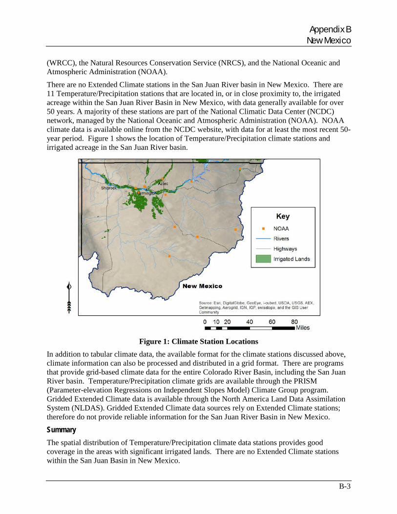
Appendix B New Mexico
B-3
(WRCC), the Natural Resources Conservation Service (NRCS), and the National Oceanic and Atmospheric Administration (NOAA).
There are no Extended Climate stations in the San Juan River basin in New Mexico. There are 11 Temperature/Precipitation stations that are located in, or in close proximity to, the irrigated acreage within the San Juan River Basin in New Mexico, with data generally available for over 50 years. A majority of these stations are part of the National Climatic Data Center (NCDC) network, managed by the National Oceanic and Atmospheric Administration (NOAA). NOAA climate data is available online from the NCDC website, with data for at least the most recent 50-year period. Figure 1 shows the location of Temperature/Precipitation climate stations and irrigated acreage in the San Juan River basin.
Figure 1: Climate Station Locations
In addition to tabular climate data, the available format for the climate stations discussed above, climate information can also be processed and distributed in a grid format. There are programs that provide grid-based climate data for the entire Colorado River Basin, including the San Juan River basin. Temperature/Precipitation climate grids are available through the PRISM (Parameter-elevation Regressions on Independent Slopes Model) Climate Group program. Gridded Extended Climate data is available through the North America Land Data Assimilation System (NLDAS). Gridded Extended Climate data sources rely on Extended Climate stations; therefore do not provide reliable information for the San Juan River Basin in New Mexico.
Summary The spatial distribution of Temperature/Precipitation climate data stations provides good coverage in the areas with significant irrigated lands. There are no Extended Climate stations within the San Juan Basin in New Mexico.
Appendix B New Mexico
B-4
Potential Crop Consumptive Use Methods There are many different methodologies that estimate PCU, or the amount of water that would be used for crop growth if provided with an ample water supply. They range in complexity, accuracy and data requirements. This section describes methods used in the San Juan River basin and other areas in New Mexico for CU and Losses reporting as well as other planning efforts.
The State of New Mexico currently uses the SCS TR-21 Modified Blaney-Criddle method to estimate and report PCU to Reclamation for the San Juan River Basin. The Blaney-Criddle methodologies consist of an empirical equation that relates PCU with mean air temperature and mean percentage daylight hours. The SCS TR-21 method was modified from the Original Blaney-Criddle method to reasonably estimate seasonal consumptive use. The modifications include the use of (1) climatic coefficients that are directly related to the mean air temperature for each of the consecutive short periods which constitutes the growing season and (2) coefficients which reflect the influence of the crop growth rates on consumptive use rates. The modified Blaney-Criddle crop coefficients are available from graphs in the SCS TR-21 publication for 25 crops, which were developed based on general climatic conditions representative of the Western U.S.
New Mexico previously used the Original Blaney-Criddle method to estimate PCU until moving to the TR-21 method starting with the 2001 to 2005 CU and Losses reporting period. Calibrated crop coefficients, allowing the Original Blaney-Criddle method to move seasonal values to monthly estimates, were from SCS TR-32 developed specifically for areas within New Mexico.
The ASCE Manual No. 70 recommends use of locally calibrated crop coefficients or an elevation adjustment of 10 percent increase in PCU for each 1,000 meters increase in elevation above sea level for the SCS Modified Blaney-Criddle method when using standard TR-21 crop coefficients. The adjustment corrects for lower mean temperatures that occur at higher elevations at a given level of solar radiation (i.e. mean temperatures do not reflect crops’ reactions to warm daytime temperatures and cool nights). The recommended adjustment is applied to the PCU estimate and to all crop types. New Mexico uses SCS TR-21 coefficients without this standard elevation adjustment when estimating San Juan River basin PCU.
Other methodologies, discussed in more detail below, are used in other areas of the State where data allows. Some of these methods require Extended Climate data, and can be used to estimate PCU for reporting and planning projects that do not require a longer period of climate variability.
• ASCE Standardized Penman-Monteith. This method, which is a slight simplification of the Penman-Monteith equation, consisting of two reference evapotranspiration (ET) equations, one for a short crop and one for a taller crop. Reference ET equations require daily temperature, solar radiation, vapor pressure and wind speed data. The State has used Penman-Monteith methods were Extended Climate data allows, for example in the Middle Rio Grande area.
• Hargreaves. The original Hargreaves method (1975) is a daily grass-reference radiation method that uses mean air temperature, the differential between daily maximum and minimum air temperatures, and solar radiation to estimate ET. As solar radiation is generally not available for many areas or for long historical periods, modifications were
Appendix B New Mexico
B-5
made to the original method whereby additional equations and/or tables could be used to estimate radiation; therefore creating a monthly temperature-based modified Hargreaves (or Hargreaves-Semani) method. This method is used by BIA to estimate PCU for the NIIP.
Summary Experts have documented the increased accuracy associated with daily PCU methods and have recommended their use in ASCE Manual 70. At this time, the lack of Extended Climate data in the San Juan River basin will necessitate the use of less accurate monthly methods, including Modified Blaney-Criddle and Hargreaves-Semani.
Effective Precipitation Methods Effective precipitation is the amount of precipitation during the irrigation season that is effective in satisfying a portion of PCU. Effective precipitation is used to estimate that amount of water crops could consume from a full irrigation supply. Crop Irrigation Requirement (CIR) is calculated as PCU less effective precipitation.
New Mexico uses the monthly SCS effective precipitation method outlined in TR-21 throughout the State.
Water Supply Data Availability Climate data, crop type and acreage are used to estimate the amount of water that a crop needs from an irrigation supply (CIR); water supply data is used to determine the amount of water the crop receives (irrigation CU). This section describes the availability of surface supply data in the San Juan River basin in New Mexico.
Diversions for most ditches in the San Juan River basin are routinely measured. Diversions to the NIIP are continuously recorded. The measured data is publically available from 2011 to the current date at http://meas.ose.state.nm.us/. There are nine active streamflow gages that provide good coverage of physical flow in the San Juan main stem and its tributaries.
Summary The availability of diversion records is sufficient to allow the estimate of irrigation CU by comparing empirical estimates of CIR with supply using an on-farm balance method. The number and location of streamflow gages are adequate for representing depleted flows in the basin.
Water Supply-Limited Consumptive Use (Irrigation CU) Methods Diversions on the main stem of the San Juan River in New Mexico generally receive a full supply; therefore New Mexico estimates that irrigation CU for the associated irrigated acreage is equal to CIR. However, acreage served from the La Plata River does not always receive a full irrigation supply. New Mexico has developed a correlation between streamflow and irrigation CU for these lands. Until gaged streamflow drops below a specific level, irrigation CU is estimated to be CIR. When the gage streamflow drops below a specific level, irrigation CU is reduced, and shortages are estimated.
Appendix B New Mexico
B-6
In some areas in New Mexico, remote sensing methods have been used that measure actual ET (consumptive use from both precipitation and irrigation) directly using an energy balance approach. Climatic factors required for this method include net radiation and heat flux conducted into the ground and air. The energy balance estimates actual ET as net radiation less the heat flux factors. The most common method for estimating actual ET using the energy balance approach is to use a satellite image-processing model.
Crop Consumptive Use Models There are several crop consumptive use models that utilize consumptive use methods and equations to estimate PCU based on climate data, acreage data, and crop type. Some models take the calculations further using effective precipitation methods to determine the portion of the PCU satisfied by precipitation and diversion records to perform an on-farm water balance, comparing CIR to water supply, resulting in irrigation CU. Other methods, specifically remote sensing methods, measure actual ET only and do not require definition of crop types or diversion records. This section describes which models have been used in the San Juan River basin for CU and Losses reporting as well as other planning efforts throughout New Mexico.
The State of New Mexico uses in-house models for their reporting of crop consumptive use in the San Juan River basin. The New Mexico CIR Fortran program input files include a temperature of earliest-moisture-use, a temperature-of-latest-moisture-use, a maximum-length-of-growing-season, and an irrigation application depth for each crop type. The CIR program includes the algorithm and recommendations outlined in TR-21, including the procedure to estimate effective precipitation. The program also allows the option to use the Original Blaney-Criddle method with TR-32 coefficients. A separate spreadsheet reads the CIR values and then estimates supply-limited consumptive use. Although diversion records are available, New Mexico does not perform and on-farm water balance to calculate irrigation CU. For acreage supplied via the main stem San Juan and Animas Rivers, the spreadsheet assumes a full supply (i.e. CIR equals irrigation CU). The spreadsheet uses measured streamflow on the La Plata River to determine the extent to which CIR can be met for acreage supplied from the La Plata River. The procedure essentially duplicates the method used by Reclamation for the CU & Losses Report (See Reclamation Appendix).
The New Mexico CIR program, coupled with spreadsheet analysis of supply-limited consumptive use, is also used in other areas of New Mexico. In addition, New Mexico has investigated Energy Balance methods using remote sensing in other basins, including:
• REEM. The Regional ET Estimation Model (REEM) is based on energy balance at the crop canopy. REEM is being investigated to use LandSat satellite images to measure actual ET (consumptive use from both precipitation and irrigation) in the Mesilla Valley.
• METRIC. Mapping Evapotranspiration at high Resolution with Internalized Calibration (METRIC) is a model that utilizes LandSat satellite imagery and the energy balance method to spatially estimate actual ET. METRIC is being investigated to measure evapotranspiration in the Middle Rio Grande basin.
• References
Appendix B New Mexico
B-7
• U.S. Bureau of Reclamation, Colorado River System Consumptive Use and Losses Reports (http://www.usbr.gov/uc/library/envdocs/reports/crs/crsul.html)
• Remote Automated Weather Station program (http://www.raws.dri.edu/)
• Parameter-elevation Regressions on Independent Slopes Model Climate Group program (http://www.prism.oregonstate.edu/)
• North America Land Data Assimilation System (http://ldas.gsfc.nasa.gov/)
• American Society of Civil Engineers (2006). “ASCE Standardized Reference Evaporation Equation”
• American Society of Civil Engineers (1990). “ASCE Manuals and Reports on Engineering Practice No. 70, Evapotranspiration and Irrigation Water Requirements”
• Soil Conservation Service (1970) “Irrigation Water Requirements Technical Release 21”
• Mapping EvapoTranspiration at high Resolution with Internalized Calibration, METRIC. (http://www.idwr.idaho.gov/GeographicInfo/METRIC/)
• Harry F. Blaney and Eldon Hanson, 1965. Consumptive Use and Water Requirements in New Mexico, Technical Report 32.
• • New Mexico Climate Center Stations, NMSU.
http://weather.nmsu.edu/climate/ws/network/nmcc/html/ • • Regional ET Estimation Model, REEM. New Mexico State University. 2004.
http://wrri.nmsu.edu/publish/other_meetings/posters2004/samani.pdf •

Appendix C Utah
Appendix C Utah
C-1
Introduction This appendix documents the methods, models and available information that Utah is currently using to estimate water supply-limited crop consumptive use (irrigation CU) for irrigated lands in the Green River and Upper Colorado River basins, and other areas of the State. This appendix provides information that supports the overall project goal of developing a coordinated long-term process among the Upper Division States (Colorado, New Mexico, Utah, and Wyoming) to estimate CU for irrigated lands in the entire Upper Colorado River basin.
Members of the URS Team met with Eric Klotz and Robert King with the Utah Division of Water Resources. The purpose of the meeting was to discuss the CU methods, available information, and modeling software and programs that Utah is currently using in the Upper Colorado River basin. Additional information was obtained from Craig Miller, also with the Utah Division of Water Resources.
Irrigated Acreage Assessment Availability and Attribution Irrigated acreage assessments define the amount of acreage that was actively irrigated and cultivated in any given year. Irrigated acreage assessments can range in the level of attribution; detailed assessments can include the attribution of:
• Crop Types • Supply Type, such as surface water, ground water, reservoir releases, or multiple sources • Supply Source, including name or unique identifier of the water permit or water right,
diversion structure, well, or reservoir • Irrigation Method, such as flood or sprinkler irrigation practices
The following describes the assessment efforts for Utah for irrigated acreage in the Upper Colorado River basins; including the availability of historical assessments, spatial format of assessments, availability of attributes, and expected assessment efforts in the future.
Land use inventory in the State of Utah began in the 1960s and continued throughout the 1970s by using large format vertical-aerial photographs and on-the-ground field surveys to label boundaries, vegetation types, and other water use information. Beginning in the 1980s, the Division of Water Resources contracted with the University of Utah Research Institute, Center for Remote Sensing and Cartography (CRSC), to prepare water-related land use inventories by using high altitude color infrared photography and laboratory interpretation, again with field checking. Beginning in 1984, the program improved by using 35mm slides, United States Geological Survey (USGS) 7-1/2 minute quadrangle maps, field-mapping using base maps produced from the 35 mm photography and a computerized GIS to process, store and retrieve land use data. Starting in 2000, the division further improved its land use program by using satellite data, USGS DOQs, NAIP and other digital images to digitize field boundaries. Once digitization is completed, field crews field check boundary files, crop types and land types for each polygon. Each 5-year assessment includes field-verified estimates of acreage, crop type, and irrigation method. Water source (i.e. specific irrigating ditch) is not identified. Upon completion, data is filed in the State Geographic Information Database (SGID) and maintained by the State Automated Geographic Reference Center (AGRC). Once the data has been published on the
Appendix C Utah
C-2
AGRC website (http://gis.utah.gov/data/water-data-services/), the data becomes available to the public and is ready to be use in preparing water-related planning studies. There is some rotation of irrigated lands at the farm level based on varying supply between wet and dry years; however the regional amount of irrigated acreage has changed little over the past 50 years. Basin-wide acreage is estimated to vary between 930,000 and 990,000 acres.
Summary The 5-year irrigated acreage assessments, coupled with field surveys, are sufficient to represent changes in irrigated acreage and crop type in the Green River and Colorado River basins in Utah. The addition of a water source (irrigating ditch) attribute would allow more detailed use of the irrigated acreage assessments for both determining irrigation CU and for long-term planning purposes.
Climate Data Availability Climate data serves as the basis for estimating the amount of water needed by a crop; climate data availability can be assessed in terms of:
• Spatial Distribution - is there a sufficient distribution of climate stations in proximity to irrigated acreage in the basin to accurately measure the climatic conditions experienced by the acreage?
• Climate Data Measured - what types of climatic factors (e.g. precipitation, wind speed, solar radiation) are recorded at each station?
Understanding the distribution and types of climate data in each basin is important because different consumptive use methods require different climate data information; and significant distance between the irrigated acreage and the climate station produces less accurate consumptive use estimates.
For purposes of this study, climate stations are categorized based on the types of data measured. Stations recording temperature and precipitation only are termed “Temperature/Precipitation” stations. Stations that record temperature and precipitation plus relative humidity, sky/cloud cover, solar radiation, wind speed and direction, and barometric pressure readings are termed “Extended Climate” stations. The following describes the climate stations in the Green River and Colorado River basins in Utah and discusses their general data availability and proximity to irrigated lands.
Climate stations in Utah are operated and maintained by several different entities including AgWeatherNetwork from Utah State University, MesoWest from the University of Utah, AgriMet Pacific Northwest Cooperative Agricultural Weather Network, Emery Water Conservancy District stations, Fruit Growers Network stations (FGNET), Soil Climate Analysis Network (SCAN) from the NRCS, and stations from NOAA/NCDC. Most of the stations operated by the universities are in the western Utah basins and include Extended Climate data.
There are 16 Extended Climate stations located in the Upper Colorado River basin in Utah; one NOAA station, one AgriMet station, five Emery Water Conservancy District (ECWCN) stations, and ten SCAN stations. There are approximately 45 Temperature/Precipitation stations that are

Appendix C Utah
C-3
located in, or in close proximity, to the irrigated acreage within the Upper Colorado River basin in Utah, with data generally available for over 50 years. A majority of these stations are part of the National Climatic Data Center (NCDC) network, managed by the National Oceanic and Atmospheric Administration (NOAA). NOAA climate data is available online from the NCDC website, with data for at least the most recent 50-year period. Table 1 lists the currently active Extended Climate stations and their associated elevation. Figure 1 shows the location of Temperature/Precipitation Climate Stations, Extended Climate stations and irrigated acreage in the Green River and Upper Colorado River basins in Utah.
Table 1: Extended Climate Station Summary Station Name Managing Entity Elevation
Eastland NRCS (SCAN) 6845
Mountain Home NRCS (SCAN) 6950
Split Mountain NRCS (SCAN) 4839
Little Red Fox NRCS (SCAN) 5397
Price NRCS (SCAN) 5647
Green River NRCS (SCAN) 4107
Harms Way NRCS (SCAN) 7049
West Summit NRCS (SCAN) 7004
Alkali Mesa NRCS (SCAN) 6451
McCracken Mesa NRCS (SCAN) 5319
Ferron ECWCD 5999
Castle Dale ECWCD 5668
Molen ECWCD 5715
Elmo ECWCD 5619
Huntington ECWCD 5850
Duchesne USBR-AgriMet 5494

Appendix C Utah
C-4
Figure 1: Climate Station Locations
In addition to tabular climate data, the available format for the climate stations discussed above, climate information can also be processed and distributed in a grid format. There are programs that provide grid-based climate data for the entire Colorado River basin.
Appendix C Utah
C-5
Temperature/Precipitation climate grids are available through the PRISM (Parameter-elevation Regressions on Independent Slopes Model) Climate Group program. Five kilometer gridded Extended Climate data is available through the North America Land Data Assimilation System (NLDAS). One kilometer gridded Extended Climate data, with the exception of wind data, is also available through the Daily Surface Weather and Climatological Summaries (Daymet). Gridded Extended Climate data sources rely on Extended Climate stations; therefore do not provide reliable information for the Green River or Upper Colorado River basins in Utah.
Summary The spatial distribution of Temperature/Precipitation climate data stations provides good coverage in the areas with significant irrigated lands. The Extended Climate stations in the basin provide good coverage in Emery County, and fair to poor coverage in other areas with significant irrigated acreage.
Potential Crop Consumptive Use Methods There are many different methodologies that estimate PCU, or the amount of water that would be used for crop growth if provided with an ample water supply. They range in complexity, accuracy and data requirements. This section describes methods used in the Upper Colorado River basin in Utah for estimating consumptive use for planning efforts.
The State of Utah has historically used the SCS TR-21 Modified Blaney-Criddle Method to estimate PCU for their internal planning and reporting of crop consumptive use. The Blaney-Criddle methodologies consist of an empirical equation that relates PCU with mean air temperature and mean percentage daylight hours. Utah uses PRISM gridded climate data in their PCU calculation. The SCS TR-21 method was modified from the Original Blaney-Criddle method to reasonably estimate seasonal consumptive use. The modifications include the use of (1) climatic coefficients that are directly related to the mean air temperature for each of the consecutive short periods which constitutes the growing season and (2) coefficients which reflect the influence of the crop growth rates on consumptive use rates. The modified Blaney-Criddle crop coefficients are available from graphs in the SCS TR-21 publication for 25 crops, which were developed based on general climatic conditions representative of the Western U.S.
The ASCE Manual No. 70 recommends the use of locally calibrated crop coefficients or an elevation adjustment of 10 percent increase in PCU for each 1,000 meters increase in elevation above sea level for the SCS Modified Blaney-Criddle method when using standard TR-21 crop coefficients. Locally calibrated coefficients were developed in 1994 and documented in Research Report 145 “Consumptive Use of Irrigated Crops in Utah” based on PCU methods using a more detailed Penman method. Those calibrated crop coefficients are used to estimate PCU in the Upper Colorado River basin in Utah.
Additional daily methodologies are used where Extended Climate data is available in other areas in the State. These methodologies include:
• ASCE Standardized Penman-Monteith. This method, which is a slight simplification of the Penman-Monteith equation, consisting of two reference evapotranspiration (ET) equations, one for a short crop and one for a taller crop. Reference ET equations require daily temperature, solar radiation, vapor pressure and wind speed data. The coefficients for both short and taller crops are provided in ASCE Manual 70.
Appendix C Utah
C-6
Summary Experts have documented the increased accuracy associated with daily PCU methods and have recommended their use in ASCE Manual 70. At this time, the lack of Extended Climate station data in some areas of the Green River and Colorado River basins in Utah necessitates the use of the less accurate Modified Blaney-Criddle method. The use of calibrated coefficients with this method increases the expected accuracy.
Effective Precipitation Methods Effective precipitation is the amount of precipitation during the irrigation season that is effective in satisfying a portion of PCU. Effective precipitation is used to estimate that amount of water crops could consume from a full irrigation supply. Crop Irrigation Requirement (CIR) is calculated as PCU less effective precipitation.
The State of Utah generally estimates effective precipitation as 80 percent of total precipitation during the irrigation season. This is a conservative estimate that has been used in a number of water studies throughout the years and has been adopted as a standard by Water Resources.
Water Supply Data Availability Climate data, crop type and acreage amounts are used to estimate the amount of water that a crop needs (potential consumptive use, PCU); water supply data is used to determine the amount of water the crop receives (irrigation CU). This section describes the availability of surface supply data in the Green River and Colorado River basins in Utah.
The Utah Division of Water Rights (UDWR) regulates the appropriation and distribution of water in the State of Utah. Some basins maintain surface water diversion records using automated recorders and field readings. Commissioners responsible for maintaining diversion records are hired by the State Engineer; however assigned commissioners are requested by, and funded by, the water users in each subbasin. For basins with commissioners, it often takes 2 to 3 years for collected diversion records to be provided to the State. In general, few diversions are recorded in the Green River and Colorado River basins in Utah.
There are 46 active streamflow gages that provide good coverage of physical flow on the Green River and Colorado River main stem and their tributaries.
Summary The lack of diversion records does not allow the estimate of supply-limited consumptive use by comparing empirical estimates of irrigated water requirement with supply using an on-farm balance method. Moving towards recording supply for a higher percentage of acreage is strongly recommended. The number and location of streamflow gages are adequate for representing depleted flows in the basin.
Water Supply-Limited Consumptive Use (Irrigation CU) Methods Utah estimates irrigation CU as a component of a basin water budget that considers measured or estimated inflows and outflows. Details of this methodology are presented in the discussion of their Utah Water Budget model below.
In some areas in Utah, remote sensing methods have been used that measure actual ET (consumptive use from both precipitation and irrigation) directly using an energy balance

Appendix C Utah
C-7
approach. Climatic factors required for this method include net radiation and heat flux conducted into the ground and air. The energy balance estimates actual ET as net radiation less the heat flux factors. The most common method for estimating actual ET using the energy balance approach is to use a satellite image-processing model.
Crop Consumptive Use Models There are several crop consumptive use models that utilize consumptive use methods and equations to estimate PCU based on climate data, acreage data, and crop type. Some models take the calculations further using effective precipitation methods to determine the portion of the PCU satisfied by precipitation and diversion records to perform an on-farm water balance, comparing CIR to water supply, resulting in irrigation CU. Some models use a basin water budget approach to estimate basin-wide water supply-limited consumptive use through an inflow/outflow approach. Other methods, specifically remote sensing methods, measure actual ET only and do not require definition of crop types or diversion records. This section describes the models used in Utah to estimate Upper Colorado River basin crop consumptive use.
The Utah Division of Water Resources (DWR) has chosen the Utah Water Budget Program to estimate irrigation CU as part of the overall basin water budget that considers measured or estimated inflows and outflows (basin water supply).
The Utah Water Budget model operates on a monthly basis using the following equation on a subbasin level:
Subbasin Yield (Natural Flow originating within the subbasin) = Outflow – Inflow + Manmade Depletions + Storage
Inflow to the stream is estimated based on measured stream gages and rainfall/runoff calculations. Where stream gages do not exist, average annual streamflows are estimated using USGS streamstats or the Water Resources developed area-altitude method. The computed annual averages are then indexed by the flows of a similar gage on a nearby stream to approximate monthly variation in the stream. Outflow is normally streamflow at the downstream gage of each subbasin. Municipal and industrial diversions, and full irrigation diversions based on CIR and estimated irrigation efficiency, are input data for each basin. If the basin inflow is able to meet municipal, industrial, and full irrigation diversions; then there are no shortages to CIR during the month and irrigation CU is equal to CIR. If basin inflow is less than diversion demands, CIR cannot be fully met and irrigation CU is reduced to reflect the available supply.
In some areas there is good coverage of streamflow gages on the main stem and major tributaries. This use of a basin inflow/outflow method mitigates the lack of measured irrigation supplies (diversion records) from surface water and ground water. The Utah Water Budget model is under final development and is expected to be run annually, and data will be published and available to the public every 5 years.
Another option to the Utah Water Budget model approach is the use of a remote sensing technique that can directly measure irrigation CU. Utah has investigated Energy Balance methods using remote sensing in other basins, including:
• METRIC. Mapping Evapotranspiration at high Resolution with Internalized Calibration (METRIC) is a model that utilizes LandSat satellite imagery and the energy balance method to spatially estimate actual ET (consumptive use from both precipitation and
Appendix C Utah
C-8
irrigation). METRIC is being investigated to measure evapotranspiration in other Utah basins. Utah is considering using METRIC to perform a pilot project in the Upper Colorado River basin where METRIC would be used to calibrate an NDVI method to calculate actual ET. The proposed project would allow the NDVI method to obtain a fairly rapid estimate of actual ET to give to the Upper Colorado River Commission; with METRIC used every few years to recalibrate the NDVI methodology to insure its accuracy.
• eLeaf. eLEAF is a Netherlands-based high-tech company that supplies reliable, quantitative data on water and vegetation on any land surface to support sustainable water use, increase food production, and protect environmental systems. eLEAF is active worldwide and has completed projects in over 30 countries. eLEAF's mission is to be the global reference in supply of reliable data on water and vegetation on any land surface to support sustainable water use, increase food production, and protect environmental systems.
References U.S. Bureau of Reclamation, Colorado River System Consumptive Use and Losses Reports (http://www.usbr.gov/uc/library/envdocs/reports/crs/crsul.html)
National Agricultural Statistics Service Cropland Data Layer (http://www.nass.usda.gov/research/Cropland/)
National Climatic Data Center (NCDC) network (http://www.ncdc.noaa.gov/)
Parameter-elevation Regressions on Independent Slopes Model Climate Group program (http://www.prism.oregonstate.edu/)
North America Land Data Assimilation System (http://ldas.gsfc.nasa.gov/)
American Society of Civil Engineers (2006). “ASCE Standardized Reference Evaporation Equation”
American Society of Civil Engineers (1990). “ASCE Manuals and Reports on Engineering Practice No. 70, Evapotranspiration and Irrigation Water Requirements”
Soil Conservation Service (1970) “Irrigation Water Requirements Technical Release 21”
Utah Department of Natural Resources. “Consumptive Use of Irrigated Crops in Utah Research Report 145”, Robert W. Hill, Utah State University
Mapping EvapoTranspiration at high Resolution with Internalized Calibration, METRIC. (http://www.idwr.idaho.gov/GeographicInfo/METRIC/)
Utah Water Rights. http://www.waterrights.utah.gov/ AgWxNet. http://climate.usurf.usu.edu/agweather.php MesoWest Climate Stations. http://mesowest.utah.edu/cgi-bin/droman/mesomap.cgi?state=UT&rawsflag=3
Appendix C Utah
C-9
AgriMet, The Pacific Northwest Cooperative Agricultural Weather Network. http://www.usbr.gov/pn/agrimet/ A Water-Related Land Use Summary Report of the State of Utah. Utah Department of Natural Resources Division of Water Resources. March 1999. http://www.water.utah.gov/planning/landuse/wrlui.pdf Water Data Services. Utah Automated Geographic Reference Center. http://gis.utah.gov/data/water-data-services/ Emery Water Conservancy District. http://www.ewcd.org/

Appendix D Wyoming
Appendix D Wyoming
D-1
Introduction This appendix documents the methods, models and available information that Wyoming is currently using to estimate water supply-limited crop consumptive use (irrigation CU) for irrigated lands in the Green River basin, and other areas of the State. This appendix provides information that supports the overall project goal of developing a coordinated long-term process among the Upper Division States (Colorado, New Mexico, Utah, and Wyoming) to estimate CU for irrigated lands in the entire Upper Colorado River basin.
Members of the URS Team met with Steve Wolff, Colorado River Coordinator for the Wyoming State Engineer’s Office, to discuss the CU methods, available information, and modeling software/programs that Wyoming is currently using in the Upper Colorado River basin.
Irrigated Acreage Assessment Availability and Attribution Irrigated acreage assessments define the amount of acreage that was actively irrigated and cultivated in any given year. Irrigated acreage assessments can range in the level of attribution; detailed assessments can include the attribution of:
• Crop Types • Supply Type, such as surface water, ground water, reservoir releases, or multiple sources • Supply Source, including name or unique identifier of the water permit or water right,
diversion structure, well, or reservoir • Irrigation Method, such as flood or sprinkler irrigation practices
The following describes the assessment efforts for irrigated acreage in the Green River Basin in Wyoming, including the availability of historical assessments, spatial format of assessments, availability of attributes, and expected assessment efforts in the future.
Wyoming conducted a survey of irrigated lands in the 1980s. Areas of irrigated acreage were determined and tabulated, but this early survey was not digitized into a GIS coverage. Reclamation delineated basin-wide irrigated lands on USGS 7.5’ quad maps in Wyoming, along with the other Upper Basin states, in early the 1990s. Wyoming identified basin-wide irrigated acreage using a GIS platform to support the Green River Basin Plan in the late 1990s. This assessment broadly identified irrigated areas, but did not include other attributes. A separate GIS point coverage was created that generally assigned water right permits to irrigated areas. This resulted in a many to many relationship that was used for the initial basin planning effort; however acreage from this assessment was not able to be tied directly to a water source (ditch river headgate). A more detailed assessment of irrigated acreage for the Green River Basin was completed in 2009 during the development of the Wyoming Water Rights Attribution Geodatabase (WYWRAG)and updated in 2013 This assessment defined more detailed irrigated parcels plus assigned water permits or water rights and river headgate source. A refinement of the irrigated lands layer was recently completed as part of the State’s remote sensing program. The wet year acreage estimates were very similar to the ones developed in 2009, while the dry year estimates were significantly lower.
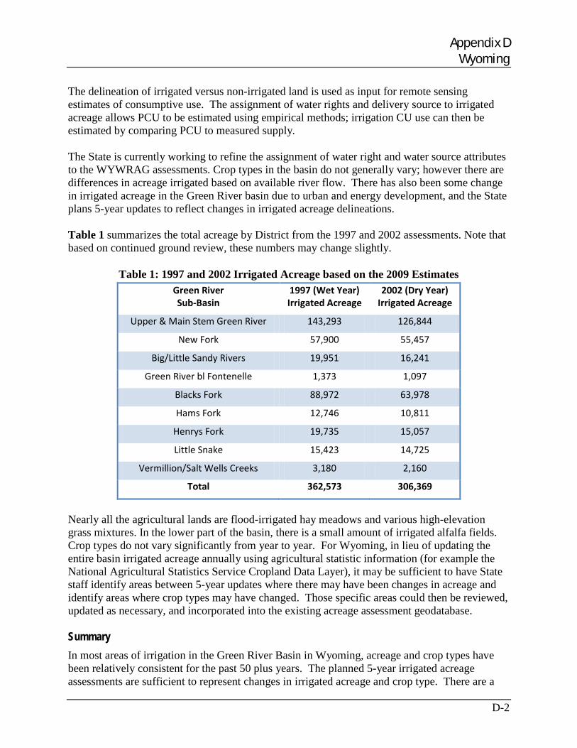
Appendix D Wyoming
D-2
The delineation of irrigated versus non-irrigated land is used as input for remote sensing estimates of consumptive use. The assignment of water rights and delivery source to irrigated acreage allows PCU to be estimated using empirical methods; irrigation CU use can then be estimated by comparing PCU to measured supply. The State is currently working to refine the assignment of water right and water source attributes to the WYWRAG assessments. Crop types in the basin do not generally vary; however there are differences in acreage irrigated based on available river flow. There has also been some change in irrigated acreage in the Green River basin due to urban and energy development, and the State plans 5-year updates to reflect changes in irrigated acreage delineations. Table 1 summarizes the total acreage by District from the 1997 and 2002 assessments. Note that based on continued ground review, these numbers may change slightly.
Table 1: 1997 and 2002 Irrigated Acreage based on the 2009 Estimates Green River Sub-Basin
1997 (Wet Year) Irrigated Acreage
2002 (Dry Year) Irrigated Acreage
Upper & Main Stem Green River 143,293 126,844
New Fork 57,900 55,457
Big/Little Sandy Rivers 19,951 16,241
Green River bl Fontenelle 1,373 1,097
Blacks Fork 88,972 63,978
Hams Fork 12,746 10,811
Henrys Fork 19,735 15,057
Little Snake 15,423 14,725
Vermillion/Salt Wells Creeks 3,180 2,160
Total 362,573 306,369
Nearly all the agricultural lands are flood-irrigated hay meadows and various high-elevation grass mixtures. In the lower part of the basin, there is a small amount of irrigated alfalfa fields. Crop types do not vary significantly from year to year. For Wyoming, in lieu of updating the entire basin irrigated acreage annually using agricultural statistic information (for example the National Agricultural Statistics Service Cropland Data Layer), it may be sufficient to have State staff identify areas between 5-year updates where there may have been changes in acreage and identify areas where crop types may have changed. Those specific areas could then be reviewed, updated as necessary, and incorporated into the existing acreage assessment geodatabase. Summary In most areas of irrigation in the Green River Basin in Wyoming, acreage and crop types have been relatively consistent for the past 50 plus years. The planned 5-year irrigated acreage assessments are sufficient to represent changes in irrigated acreage and crop type. There are a
Appendix D Wyoming
D-3
few areas where energy and urban development may warrant more frequent updates. Depending on levels of development, it may be important to delineate irrigated parcel boundaries in these areas more frequently than every five years.
Climate Station Data Availability
Climate data serves as the basis for estimating the amount of water needed by a crop; climate data availability can be assessed in terms of:
• Spatial Distribution - is there a sufficient distribution of climate stations in proximity to irrigated acreage in the basin to accurately measure the climatic conditions experienced by the acreage?
• Climate Data Measured - what types of climatic factors (e.g. precipitation, wind speed, solar radiation) are recorded at each station?
Understanding the distribution and types of climate data in each basin is important because different consumptive use methods require different climate data information; and significant distance between the irrigated acreage and the climate station produces less accurate consumptive use estimates.
For purposes of this study, climate stations are categorized based on the types of data measured. Stations recording temperature and precipitation only are termed “Temperature/Precipitation” stations. Stations that record temperature and precipitation plus relative humidity, sky/cloud cover, solar radiation, wind speed and direction, and barometric pressure readings are termed “Extended Climate” stations. The following describes the climate stations in Green River Basin in Wyoming and discusses their general data availability and proximity to irrigated lands.
Climate stations in Wyoming are operated and maintained by several different entities including the Wyoming State Engineer’s Office, National Weather Service (NWS), U.S. Bureau of Land Management (BLM), Wyoming Department of Environmental Quality (WYDEQ), U.S. Geological Survey (USGS), the Natural Resources Conservation Service (NRCS), and the National Oceanic and Atmospheric Administration (NOAA). There are 12 Extended Climate stations in the Green River Basin with data available for some of the stations beginning in the late 1980s. Stations recently installed by the SEO are in close proximity to irrigated lands, with the primary purpose of these stations to provide climate data for use in consumptive use estimates and modeling. Close to 40 Temperature/Precipitation stations are located in, or in close proximity to, the Green River Basin, with data generally available for over 50 years. A majority of these stations are part of the National Climatic Data Center (NCDC) network, managed by the National Oceanic and Atmospheric Administration (NOAA). NOAA climate data is available online from the NCDC website, with data for at least the most recent 50-year period. A survey of the NOAA/NWS (mostly coop gages) by the SEO has deemed many of these as unusable in consumptive use work based primarily on their location or condition.
Table 2 lists the currently active Extended Climate stations and their associated elevation and first observation dates. Figure 1 provides a map of the Extended Climate stations and Temperature/ Precipitation stations plus the 1997 irrigated acreage to provide a visual of the proximity of these stations to the irrigated acreage. The Automated Surface Observing Systems stations are maintained for air traffic, and are generally not located in areas of irrigated acreage and are not representative of the higher tributaries. Likewise, the Wyoming Visibility Monitoring
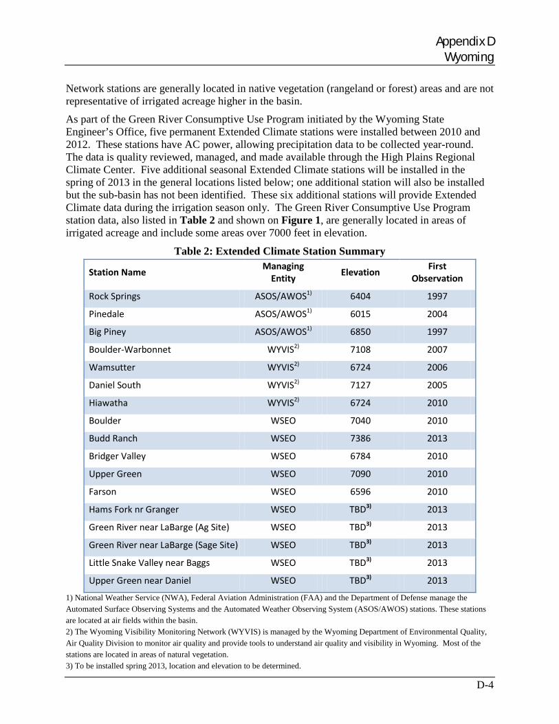
Appendix D Wyoming
D-4
Network stations are generally located in native vegetation (rangeland or forest) areas and are not representative of irrigated acreage higher in the basin.
As part of the Green River Consumptive Use Program initiated by the Wyoming State Engineer’s Office, five permanent Extended Climate stations were installed between 2010 and 2012. These stations have AC power, allowing precipitation data to be collected year-round. The data is quality reviewed, managed, and made available through the High Plains Regional Climate Center. Five additional seasonal Extended Climate stations will be installed in the spring of 2013 in the general locations listed below; one additional station will also be installed but the sub-basin has not been identified. These six additional stations will provide Extended Climate data during the irrigation season only. The Green River Consumptive Use Program station data, also listed in Table 2 and shown on Figure 1, are generally located in areas of irrigated acreage and include some areas over 7000 feet in elevation.
Table 2: Extended Climate Station Summary
Station Name Managing Entity Elevation First
Observation
Rock Springs ASOS/AWOS1) 6404 1997
Pinedale ASOS/AWOS1) 6015 2004
Big Piney ASOS/AWOS1) 6850 1997
Boulder-Warbonnet WYVIS2) 7108 2007
Wamsutter WYVIS2) 6724 2006
Daniel South WYVIS2) 7127 2005
Hiawatha WYVIS2) 6724 2010
Boulder WSEO 7040 2010
Budd Ranch WSEO 7386 2013
Bridger Valley WSEO 6784 2010
Upper Green WSEO 7090 2010
Farson WSEO 6596 2010
Hams Fork nr Granger WSEO TBD3) 2013
Green River near LaBarge (Ag Site) WSEO TBD3) 2013
Green River near LaBarge (Sage Site) WSEO TBD3) 2013
Little Snake Valley near Baggs WSEO TBD3) 2013
Upper Green near Daniel WSEO TBD3) 2013
1) National Weather Service (NWA), Federal Aviation Administration (FAA) and the Department of Defense manage the Automated Surface Observing Systems and the Automated Weather Observing System (ASOS/AWOS) stations. These stations are located at air fields within the basin. 2) The Wyoming Visibility Monitoring Network (WYVIS) is managed by the Wyoming Department of Environmental Quality, Air Quality Division to monitor air quality and provide tools to understand air quality and visibility in Wyoming. Most of the stations are located in areas of natural vegetation. 3) To be installed spring 2013, location and elevation to be determined.
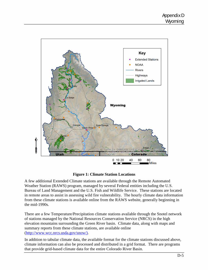
Appendix D Wyoming
D-5
Figure 1: Climate Station Locations
A few additional Extended Climate stations are available through the Remote Automated Weather Station (RAWS) program, managed by several Federal entities including the U.S. Bureau of Land Management and the U.S. Fish and Wildlife Service. These stations are located in remote areas to assist in assessing wild fire vulnerability. The hourly climate data information from these climate stations is available online from the RAWS website, generally beginning in the mid-1990s. There are a few Temperature/Precipitation climate stations available through the Snotel network of stations managed by the National Resources Conservation Service (NRCS) in the high elevation mountains surrounding the Green River basin. Climate data, along with maps and summary reports from these climate stations, are available online (http://www.wcc.nrcs.usda.gov/snow/).
In addition to tabular climate data, the available format for the climate stations discussed above, climate information can also be processed and distributed in a grid format. There are programs that provide grid-based climate data for the entire Colorado River Basin.
Appendix D Wyoming
D-6
Temperature/Precipitation climate grids are available through the PRISM (Parameter-elevation Regressions on Independent Slopes Model) Climate Group program. Gridded Extended Climate data is available through the North America Land Data Assimilation System (NLDAS).
Summary The spatial distribution of the Temperature/Precipitation and Extended Climate data stations provide good coverage of the basin, with increased density of stations near irrigated lands in areas under about 6800 feet elevation. The Extended Climate stations recently installed in through the State Engineer’s Office and most of the NOAA stations are located within or very near irrigated fields. The number and density of Extended Climate stations appears to be sufficient to determine crop consumptive use for irrigated acreage generally below 7500 feet elevation using the more data-intensive daily consumptive use methods in and to support calibration and verification of remote sensing methods in most areas of the basin. Around 20 percent of the irrigated acreage in the basin is above 7500 feet; therefore additional Extended Climate stations above 7500 feet may be warranted.
Quality review and correction of daily Extended Climate station data is recommended prior to use and standard procedures have been developed and documented in ASCE Standardized Reference Evaporation Equation Handbook. Although standardized, this quality review can be time-consuming and requires more effort than using monthly temperature and precipitation data, which is reviewed prior to publication and does not require additional quality control.
Potential Crop Consumptive Use Methods There are many different methodologies that estimate PCU, or the amount of water that would be used for crop growth if provided with an ample water supply. They range in complexity, accuracy and data requirements. This section describes methods used in the Green River Basin in Wyoming for CU and Losses reporting as well as other planning efforts.
The State of Wyoming has not prepared a basin-wide CU and Losses Report; they do not use, nor have they endorsed, Reclamation’s CU and Losses Report. As discussed in the Reclamation Appendix, Reclamation develops Wyoming’s section of the CU and Losses Report using the SCS TR-21 Modified Blaney-Criddle method with TR-21 published crop coefficients. Reclamation does not apply the standard elevation adjustment discussed below.
The State of Wyoming uses several empirical consumptive use methods to determine PCU in the Green River Basin and throughout Wyoming for planning purposes, including FAO-24 and SCS TR-21 Modified Blaney-Criddle, Hargreaves, and ASCE Standardized Penman. In addition, they have used the remote sensing energy balance method, METRIC, to estimate actual ET (consumptive use from both precipitation and irrigation). The use of METRIC and other remote sensing techniques is discussed further in the Remote Sensing Techniques appendix.
The Blaney-Criddle methodologies consist of empirical equations that relate PCU with mean air temperature and mean percentage daylight hours. The SCS TR-21 method was modified from the Original Blaney-Criddle method to reasonably estimate seasonal consumptive use. The modifications include the use of (1) climatic coefficients that are directly related to the mean air temperature for each of the consecutive short periods which constitutes the growing season and (2) coefficients which reflect the influence of the crop growth rates on consumptive use rates. The FAO-24 Blaney-Criddle method was modified from the Original Blaney-Criddle method to
Appendix D Wyoming
D-7
better account for the effect of humidity, sunshine and wind on crop PCU while still using the temperature and daylight parameters from the original method.
The ASCE Manual No. 70 recommends an elevation adjustment of 10 percent increase in PCU for each 1,000 meters increase in elevation above sea level for monthly methods, including FAO-24 and SCS Modified Blaney-Criddle method when using standard (non-calibrated) crop coefficients. The adjustment corrects for lower mean temperatures that occur at higher elevations at a given level of solar radiation (i.e. mean temperatures do not reflect crops’ reactions to warm daytime temperatures and cool nights). The recommended adjustment is applied to the PCU estimate and to all crop types.
The State of Wyoming has used published average monthly estimates of PCU based on FAO-24 Blaney-Criddle, calibrated to local conditions (Pochop et. al, 1992, WWRC #92-06). These average monthly estimates have been widely used when average estimates are acceptable for planning purposes. The method has not been used for more detailed studies that need to consider climate variability or for studies that look at supply-limited consumptive use and associated shortages.
More recently, the SCS TR-21 Blaney-Criddle method with standard elevation adjustments has been used to estimate historical consumptive use in basin planning efforts and to identify shortages and water availability for new storage projects throughout Wyoming, including in the Green River Basin. Because of the historical temporal and spatial availability of the input data requirements (i.e. temperature and precipitation data have long-term availability), this method allows for a longer planning horizon, representing more climate and hydrologic variation.
Daily methodologies, discussed in more detail below, are also used within the State where data allows. These methods, which require Extended Climate data, can be used to estimate PCU for reporting and planning projects that do not require a longer period of climate variability. As the State installs and supports more Extended Climate stations, they plan to replace the less accurate monthly Blaney-Criddle methods with more accurate daily methods.
• ASCE Standardized Penman-Monteith. This method, which is a slight simplification of the Penman-Monteith equation, consisting of two reference evapotranspiration (ET) equations, one for a short crop and one for a taller crop. Reference ET equations require daily temperature, solar radiation, vapor pressure and wind speed data. The coefficients for both short and taller crops are provided in ASCE Manual 70. The State plans to use this method as their standard in the Green River Basin in areas where sufficient Extended Climate data is available.
• Hargreaves. The original Hargreaves method (1975) is a daily grass-reference radiation method that uses mean air temperature, the differential between daily maximum and minimum air temperatures, and solar radiation to estimate ET. As solar radiation is generally not available for many areas or for long historical periods, modifications were made to the original method whereby additional equations and/or tables could be used to estimate radiation; therefore creating a temperature-based modified Hargreaves (or Hargreaves-Semani) method. This method has not been widely used in the Green River basin, but in other basins in Wyoming.
Appendix D Wyoming
D-8
Summary Although the Blaney-Criddle methodologies may be preferred for large-scale consumptive use modeling and reporting especially when estimating historical crop demands over a period representing climate variability (e.g. to demonstrate a purpose and needs for a new reservoir), there is sufficient data from Extended Climate stations to use a more data-intensive methodology for annual CU and Losses reporting in most areas of the Green River Basin. There are essentially no additional costs associated with a more detailed daily method beyond the quality control of the daily data, discussed above. Experts have documented the increased accuracy associated with daily methods and have recommended their use in ASCE Manual 70.
The use of METRIC to directly measure actual ET is important in Wyoming because of the limited availability of water supply data (diversion records). Estimates of PCU are still required to allow a comparison to METRIC results for purposes of identifying shortages. METRIC results for areas with a full supply can also be used to develop locally calibrated coefficients for the ASCE Penman method.
Effective Precipitation Methods Effective precipitation is the amount of precipitation during the irrigation season that is effective in satisfying a portion of PCU. Effective precipitation is used to estimate that amount of water crops could consume from a full irrigation supply. Crop Irrigation Requirement (CIR) is calculated as PCU less effective precipitation.
The State of Wyoming historically estimated effective precipitation to be 80 percent of irrigation season rainfall (Pochop et. al, 1992, WWRC #92-06). More recently in the Green River Basin, they have used the SCS effective precipitation method outlined in TR-21.
Water Supply Data Availability Climate data, crop type and acreage are used to estimate the amount of water that a crop needs from an irrigation supply (CIR); water supply data is used to determine the amount of water the crop receives (irrigation CU). This section describes the availability of surface water supply data in the Green River Basin in Wyoming.
The State Engineer’s Office Board of Control Division is responsible for the administration and regulation of the waters of the state based on the Prior Appropriation System. The Division IV Superintendent, Hydrographers, and Water Commissioners are responsible for administering the water rights and permits in the Green River Basin and taking measurements of streamflow and diversions in their basin. The responsibility of recording diversions extends to both surface and ground water use, however there is very little ground water used for irrigation in the Green River Basin, therefore this discussion will focus on surface water diversions.
In general, headgate diversions on tributaries and main stem reaches that do not require active administration are not measured and recorded. There are over 1,350 active headgates in the basin. About 150 diversion structures are continuous measured and approximately 600 are spot measured one or more times annually. Figure 2 shows locations of measured diversions as of 2010 (Green River Decision Support System Feasibility Study).
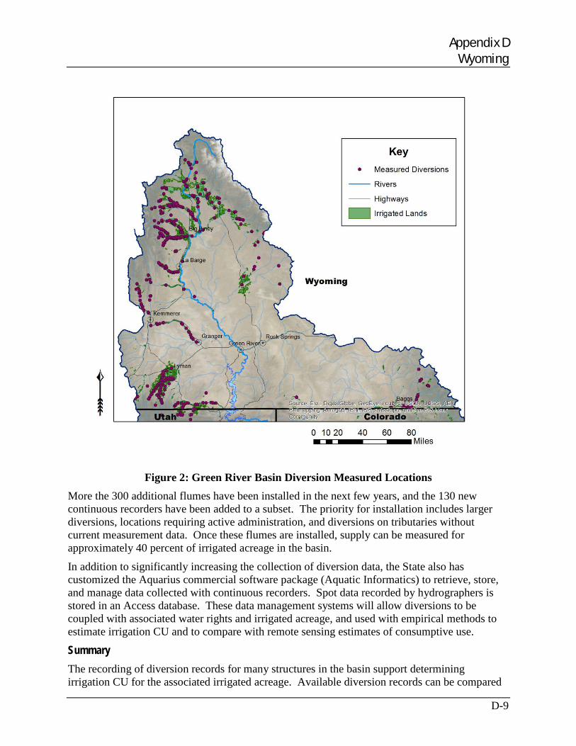
Appendix D Wyoming
D-9
Figure 2: Green River Basin Diversion Measured Locations
More the 300 additional flumes have been installed in the next few years, and the 130 new continuous recorders have been added to a subset. The priority for installation includes larger diversions, locations requiring active administration, and diversions on tributaries without current measurement data. Once these flumes are installed, supply can be measured for approximately 40 percent of irrigated acreage in the basin.
In addition to significantly increasing the collection of diversion data, the State also has customized the Aquarius commercial software package (Aquatic Informatics) to retrieve, store, and manage data collected with continuous recorders. Spot data recorded by hydrographers is stored in an Access database. These data management systems will allow diversions to be coupled with associated water rights and irrigated acreage, and used with empirical methods to estimate irrigation CU and to compare with remote sensing estimates of consumptive use.
Summary The recording of diversion records for many structures in the basin support determining irrigation CU for the associated irrigated acreage. Available diversion records can be compared
Appendix D Wyoming
D-10
to empirical estimates of irrigated water requirement using an on-farm balance method. Supply-limited crop consumptive use based on recorded diversions can be used to estimate consumptive use for acreage without a measured supply based on criteria such as similar water right priorities or proximity (i.e. tributaries with similar physical supply limitations). Although the procedure to estimate supply-limited consumptive use based on nearby diversions is acceptable, moving towards recording supply for a higher percentage of acreage is strongly recommended.
Water Supply-Limited Consumptive Use (Irrigation CU) Methods Wyoming uses measured diversions to perform on-farm water balances, comparing CIR to water supply on a ditch-by-ditch basis to estimate irrigation CU, where diversions records are available. As discussed above, Wyoming’s recent irrigated acreage assessments tie acreage directly to a ditch. For ditches with measured diversions, estimates of conveyance and maximum application efficiency are used to determine the portion of water diverted at the river that is available to the crop. If water available to the crop is greater or equal to CIR; then irrigation CU is equal to CIR and there is no supply shortage. If water available to the crop is less than CIR; then water available to the crop is irrigation CU and shortage is calculated as CIR less irrigation CU.
Because many ditch diversions are not routinely measured, irrigation CU for much of the acreage is estimated by assuming monthly shortages calculated for measured ditches can be used to represent shortages to other ditch systems in the same geographic region. These estimated shortages are then used to estimate irrigation CU.
In some areas in Wyoming including the Green River Basin, remote sensing methods have been used that measure actual ET (consumptive use from both precipitation and irrigation) directly using an energy balance approach. Climatic factors required for this method include net radiation and heat flux conducted into the ground and air. The energy balance estimates actual ET as net radiation less the heat flux factors. The most common method for estimating actual ET using the energy balance approach is to use a satellite image-processing model. The State is in the process of finalizing actual ET estimates for the Green River basin using the METRIC energy balance approach. The goal is to perform a METRIC analysis every five years.
Crop Consumptive Use Models There are several crop consumptive use models that utilize consumptive use methods and equations to estimate PCU based on climate data, acreage data, and crop type. Some models take the calculations further using effective precipitation methods to determine the portion of the PCU satisfied by precipitation and diversion records to perform an on-farm water balance, comparing CIR to water supply, resulting in irrigation CU. Other methods, specifically remote sensing methods, measure irrigation CU and do not require definition of crop types or diversion records. As discussed above, remote sensing methods will still require empirical estimated PCU and estimates of effective precipitation, so diversion-caused depletions and shortages can be reported. This section describes which models have been used for planning efforts throughout Wyoming.
The State of Wyoming has used several models to estimate PCU. Recently they have used StateCU to estimate PCU and supply-limited consumptive use in the Green River Basin. StateCU is a publically available, Fortran-based program with an associated graphical user interface (GUI) that estimates PCU and water supply-limited consumptive use using daily or monthly
Appendix D Wyoming
D-11
methods. The crop consumptive use methods employed in the program include the SCS TR-21 Modified, Original Blaney-Criddle, and Pochop Bluegrass methods with calculations on a monthly basis; and the Original Penman-Monteith and ASCE Standardized Penman-Monteith methods with calculations on a daily basis. The model also supports several methods to determine effective precipitation, allows for standard elevation adjustments as recommended by ASCE Manual 70, and allows the use of locally-calibrated crop coefficients. PCU can be estimated for various crops at a location based on climate data from one or more climate stations.
StateCU has also been used to estimate water supply-limited consumptive use for the entire Green River basin. StateCU provides an option to determine supply-limited consumptive use and associated shortages where diversion records are available, and the use the shortage information to “prorate” CIR to estimate supply-limited consumptive use for acreage without supply measurements.
Estimates of irrigation CU in the Green River Basin have also been developed using METRIC. Mapping Evapotranspiration at high Resolution with Internalized Calibration (METRIC) is a model that utilizes satellite imagery and the energy balance method to spatially estimate irrigation CU. LandSat satellite imagery records thermal infrared light that is used in the energy balance to determine net radiation and the model utilizes local climate data to determine the remaining factors in the energy balance equation and calibrate the ET results. The Wyoming State Engineer’s office is planning on using METRIC to provide consumptive use estimates in the Green River Basin every 5 years concurrent with StateCU analyses.
The NDVI methodology utilizes the normalized difference vegetative index (NDVI) measure of greenness within satellite images to estimate irrigation CU for irrigated fields and native vegetation. Wyoming has plans to apply the NDVI approach to compare with METRIC results in the Green River Basin and, potentially, use between the years that METRIC estimates are made.
Additional consumptive use models are used within the State; for example, models developed by universities/research institutes and models designed for field-level or single season applications. Other models include:
• ArcGIS ET Calculator Model. The ArcGIS ET Calculator Model is a GIS-based ET calculation model which is expected to use the ASCE Standardized, the FAO-24 Blaney-Criddle, and the Hargreaves-Samani methods to calculate and spatially distribute ET and CIR. Five climatic factors, common to some or all of the consumptive use methods, are input to determine reference ET (ETr); including solar radiation, soil heat flux, temperature, wind speed and vapor pressure. Precipitation data is also required as an input to determine CIR. The climate data is spatially distributed across the State with a GIS grid layer. In addition, crop coefficients, either Pochop calibrated coefficients or standard grass reference coefficients, are also spatially distributed across the State. The model calculates ETr using the climate data grid resulting in spatial reference ETr. Using the coefficient and ETr grids, crop consumptive use is spatially calculated and can be determined for a specified area. The model can also calculate CIR using spatial precipitation data. The model is currently under development at the University of
Appendix D Wyoming
D-12
Wyoming in response to the Water Research Program 2010 request for proposals on the Consumptive Use of Water from Irrigated Lands project.
• NRCS ET Calculator Spreadsheet Model. Wyoming uses the NRCS ET Calculator Spreadsheet Model (Snyder and Eching, 2003) in the North Platte Basin to determine and report changes in depletions as required by the Platte River Recovery Program. The spreadsheet includes average monthly estimates of crop ET, native vegetation ET, and surface evaporation depletions for eight regions within the Platte River basin. The model is used to quantify changes in depletions due to changes in land use, for example the change in consumptive use for a new pond compared to previous native vegetation. When development is complete, the ArcGIS ET Calculator is expected to replace this spreadsheet model.
References U.S. Bureau of Reclamation, Colorado River System Consumptive Use and Losses Reports (http://www.usbr.gov/uc/library/envdocs/reports/crs/crsul.html)
National Agricultural Statistics Service Cropland Data Layer (http://www.nass.usda.gov/research/Cropland/)
StateCU, available through Colorado’s Decision Support Systems (http://cdss.state.co.us)
Remote Automated Weather Station program (http://www.raws.dri.edu/)
National Climatic Data Center (NCDC) network (http://www.ncdc.noaa.gov/)
National Resources Conservation Service Snowtel Sites (http://www.wcc.nrcs.usda.gov/snow/)
Community Collaborative Rain, Hail and Snow (http://www.cocorahs.org/)
Parameter-elevation Regressions on Independent Slopes Model Climate Group program (http://www.prism.oregonstate.edu/)
North America Land Data Assimilation System (http://ldas.gsfc.nasa.gov/)
American Society of Civil Engineers (2006). “ASCE Standardized Reference Evaporation Equation”
American Society of Civil Engineers (1990). “ASCE Manuals and Reports on Engineering Practice No. 70, Evapotranspiration and Irrigation Water Requirements”
Soil Conservation Service (1970) “Irrigation Water Requirements Technical Release 21”
Food and Agricultural Organization of the United Nations, Rome, Italy (1998) “Crop Evapotranspiration, Guidelines for Computing Crop Water Requirements”. FAO Irrigation and Drainage Paper 56, Allen, R.G., Pereira, L.S., Raes, D., Smith, D. and M., 1998
Consumptive Use and Consumptive Irrigation Requirements in Wyoming (1992) Pochop et.al

Appendix D Wyoming
D-13
Blaney, Harry F. and W. D. Criddle (1962). Determining Consumptive Use and Irrigation Water Requirements. Agriculture Research Service, U.S. Department of Agriculture, Technical Bulletin No. 1275. Washington, D. C.: U.S. Government Printing Office. 1962.
Mapping EvapoTranspiration at high Resolution with Internalized Calibration, METRIC. (http://www.idwr.idaho.gov/GeographicInfo/METRIC/)

Appendix E Reclamation
Appendix E Reclamation
E-1
Introduction This appendix documents the methods, models and available information that the U.S. Department of Interior Bureau of Reclamation (Reclamation) is currently using to estimate water supply-limited crop consumptive use (irrigation CU) for irrigated lands in the Upper Colorado River basin to support the Consumptive Uses and Losses Report (CU and Losses Report). This appendix provides information that supports the overall project goal of developing a coordinated long-term process among the Upper Division States (Colorado, New Mexico, Utah, and Wyoming) to estimate consumptive use for irrigated lands in the entire Upper Colorado River basin. Members of the URS Team met with David Eckhardt, Physical Scientist with the Technical Services Division, and James Prairie, Hydraulic Engineer for the Upper Colorado River Basin region of Reclamation. Dave and Jim assist in the development and review of the information required for the annual CU and Losses Report. The purpose of the meeting was to discuss the consumptive use methods, available information, and modeling software/programs used by Reclamation in the annual reporting.
Reclamation has taken the lead in performing the analysis required for the CU and Losses Reporting since the early 1970s. This project provided a venue for fully documenting both the current process and the history of the development of the CU and Losses Report. Therefore, Reclamation took a lead role in the development of this appendix and it provides much more specific detail than the general overviews provided in each State appendices.
Irrigated Acreage Assessment Availability and Attribution Irrigated acreage assessments define the amount of acreage that was actively irrigated and cultivated in any given year. Irrigated acreage assessments can range in the level of attribution; detailed assessments can include the attribution of:
• Crop Types • Supply Type, such as surface water, ground water, reservoir releases, or multiple sources • Supply Source, including name or unique identifier of the water permit or water right,
diversion structure, well, or reservoir • Irrigation Method, such as flood or sprinkler irrigation practices
Irrigated acreage is estimated out of Reclamation’s Denver Technical Services Center. David Eckhardt and the Reclamation remote sensing group have generated maps of irrigation status and irrigated crop type across the Upper Colorado Basin since the early 1990s. After the development of the first Basin-wide GIS of irrigated lands in the late 1980s to early 1990s and the first Basin-wide mapping of irrigated status in 1995 using satellite imagery, Reclamation’s goal is for every part of the basin to be mapped once during each five-year CU and Losses reporting period – either by the States or Reclamation without duplication of efforts. These maps are stored in a GIS to facilitate analysis by Alan Harrison (and his predecessor Brenda Kinkel) during the calculation of consumptive water use by irrigated agriculture.
In addition to the GIS data, Reclamation has used U.S. Department of Agriculture data from the annual Agriculture Statistics Service and 5-year Census of Agriculture data to estimate irrigated crop acreage for years when the crops are not mapped with GIS. To preserve consistency with irrigation data developed throughout the entire history of the CU and Losses work (1971 through present), these three data sources are combined based on specific rules to arrive at irrigated acreage each year.
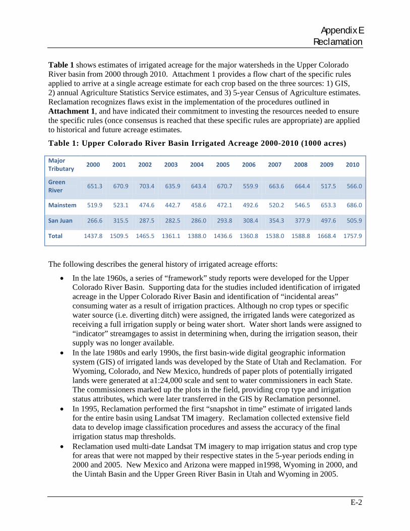
Appendix E Reclamation
E-2
Table 1 shows estimates of irrigated acreage for the major watersheds in the Upper Colorado River basin from 2000 through 2010. Attachment 1 provides a flow chart of the specific rules applied to arrive at a single acreage estimate for each crop based on the three sources: 1) GIS, 2) annual Agriculture Statistics Service estimates, and 3) 5-year Census of Agriculture estimates. Reclamation recognizes flaws exist in the implementation of the procedures outlined in Attachment 1, and have indicated their commitment to investing the resources needed to ensure the specific rules (once consensus is reached that these specific rules are appropriate) are applied to historical and future acreage estimates.
Table 1: Upper Colorado River Basin Irrigated Acreage 2000-2010 (1000 acres)
Major Tributary 2000 2001 2002 2003 2004 2005 2006 2007 2008 2009 2010
Green River 651.3 670.9 703.4 635.9 643.4 670.7 559.9 663.6 664.4 517.5 566.0
Mainstem 519.9 523.1 474.6 442.7 458.6 472.1 492.6 520.2 546.5 653.3 686.0
San Juan 266.6 315.5 287.5 282.5 286.0 293.8 308.4 354.3 377.9 497.6 505.9
Total 1437.8 1509.5 1465.5 1361.1 1388.0 1436.6 1360.8 1538.0 1588.8 1668.4 1757.9
The following describes the general history of irrigated acreage efforts:
• In the late 1960s, a series of “framework” study reports were developed for the Upper Colorado River Basin. Supporting data for the studies included identification of irrigated acreage in the Upper Colorado River Basin and identification of “incidental areas” consuming water as a result of irrigation practices. Although no crop types or specific water source (i.e. diverting ditch) were assigned, the irrigated lands were categorized as receiving a full irrigation supply or being water short. Water short lands were assigned to “indicator” streamgages to assist in determining when, during the irrigation season, their supply was no longer available.
• In the late 1980s and early 1990s, the first basin-wide digital geographic information system (GIS) of irrigated lands was developed by the State of Utah and Reclamation. For Wyoming, Colorado, and New Mexico, hundreds of paper plots of potentially irrigated lands were generated at a1:24,000 scale and sent to water commissioners in each State. The commissioners marked up the plots in the field, providing crop type and irrigation status attributes, which were later transferred in the GIS by Reclamation personnel.
• In 1995, Reclamation performed the first “snapshot in time” estimate of irrigated lands for the entire basin using Landsat TM imagery. Reclamation collected extensive field data to develop image classification procedures and assess the accuracy of the final irrigation status map thresholds.
• Reclamation used multi-date Landsat TM imagery to map irrigation status and crop type for areas that were not mapped by their respective states in the 5-year periods ending in 2000 and 2005. New Mexico and Arizona were mapped in1998, Wyoming in 2000, and the Uintah Basin and the Upper Green River Basin in Utah and Wyoming in 2005.
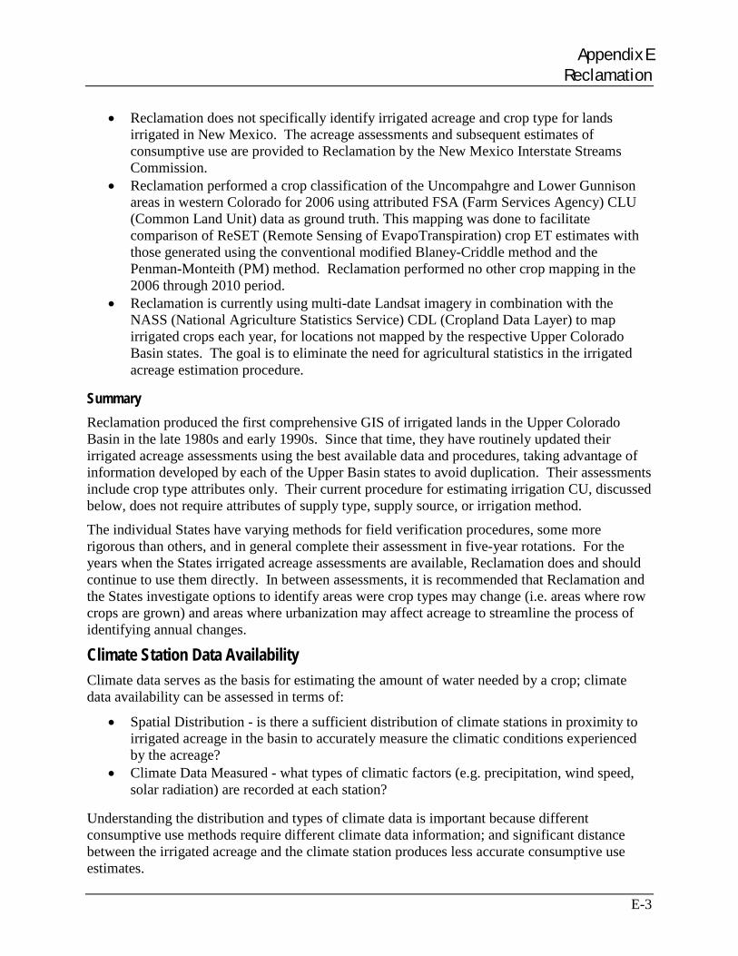
Appendix E Reclamation
E-3
• Reclamation does not specifically identify irrigated acreage and crop type for lands irrigated in New Mexico. The acreage assessments and subsequent estimates of consumptive use are provided to Reclamation by the New Mexico Interstate Streams Commission.
• Reclamation performed a crop classification of the Uncompahgre and Lower Gunnison areas in western Colorado for 2006 using attributed FSA (Farm Services Agency) CLU (Common Land Unit) data as ground truth. This mapping was done to facilitate comparison of ReSET (Remote Sensing of EvapoTranspiration) crop ET estimates with those generated using the conventional modified Blaney-Criddle method and the Penman-Monteith (PM) method. Reclamation performed no other crop mapping in the 2006 through 2010 period.
• Reclamation is currently using multi-date Landsat imagery in combination with the NASS (National Agriculture Statistics Service) CDL (Cropland Data Layer) to map irrigated crops each year, for locations not mapped by the respective Upper Colorado Basin states. The goal is to eliminate the need for agricultural statistics in the irrigated acreage estimation procedure.
Summary Reclamation produced the first comprehensive GIS of irrigated lands in the Upper Colorado Basin in the late 1980s and early 1990s. Since that time, they have routinely updated their irrigated acreage assessments using the best available data and procedures, taking advantage of information developed by each of the Upper Basin states to avoid duplication. Their assessments include crop type attributes only. Their current procedure for estimating irrigation CU, discussed below, does not require attributes of supply type, supply source, or irrigation method.
The individual States have varying methods for field verification procedures, some more rigorous than others, and in general complete their assessment in five-year rotations. For the years when the States irrigated acreage assessments are available, Reclamation does and should continue to use them directly. In between assessments, it is recommended that Reclamation and the States investigate options to identify areas were crop types may change (i.e. areas where row crops are grown) and areas where urbanization may affect acreage to streamline the process of identifying annual changes.
Climate Station Data Availability Climate data serves as the basis for estimating the amount of water needed by a crop; climate data availability can be assessed in terms of:
• Spatial Distribution - is there a sufficient distribution of climate stations in proximity to irrigated acreage in the basin to accurately measure the climatic conditions experienced by the acreage?
• Climate Data Measured - what types of climatic factors (e.g. precipitation, wind speed, solar radiation) are recorded at each station?
Understanding the distribution and types of climate data is important because different consumptive use methods require different climate data information; and significant distance between the irrigated acreage and the climate station produces less accurate consumptive use estimates.
Appendix E Reclamation
E-4
For purposes of this study, climate stations are categorized based on the types of data measured. Stations recording temperature and precipitation only are termed “Temperature/Precipitation” stations. Stations that record temperature and precipitation plus relative humidity, sky/cloud cover, solar radiation, wind speed and direction, and barometric pressure readings are termed “Extended Climate” stations. Climate data availability is outlined in each of the State’s appendices. Reclamation currently uses the Cooperative Observer Network (COOP) Temperature/Precipitation stations shown on Figure 1 to estimate PCU. These stations are maintained and data collected by the National Weather Service.
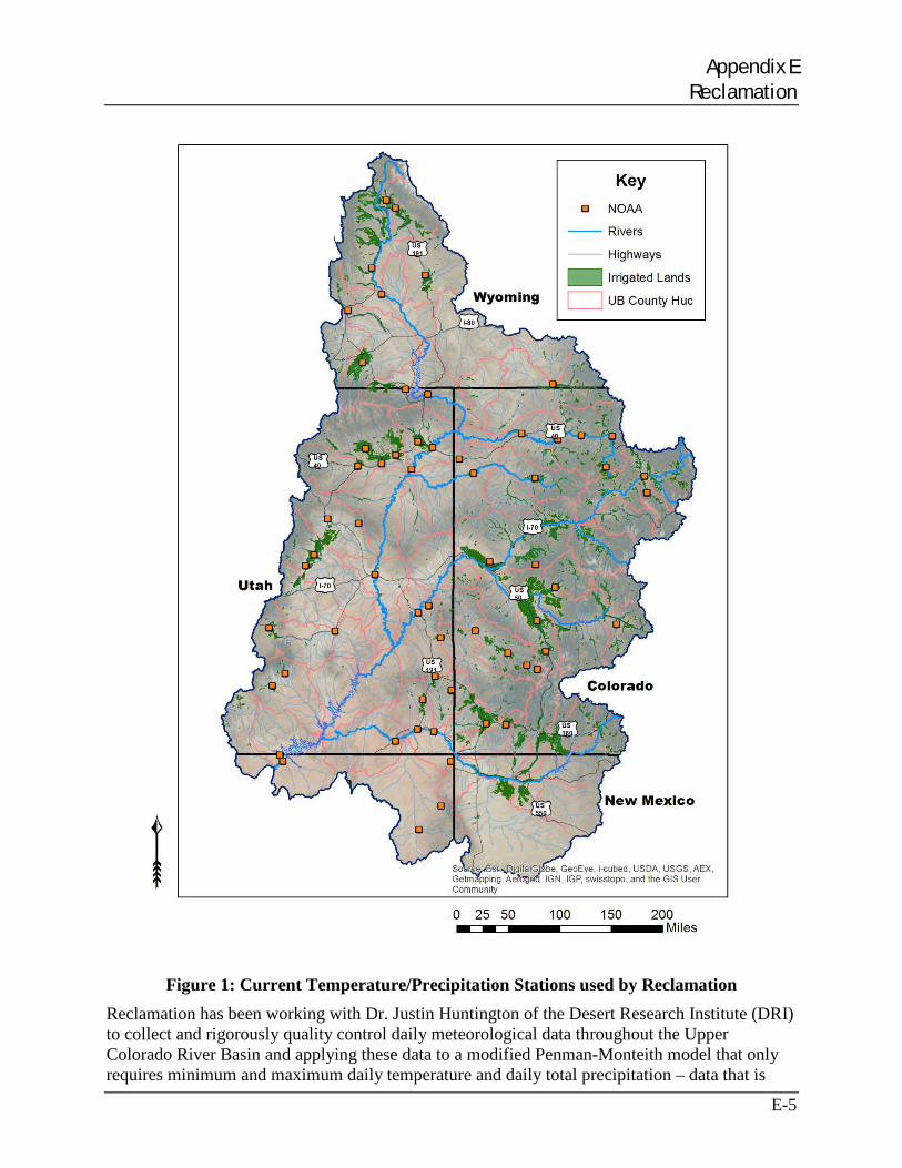
Appendix E Reclamation
E-5
Figure 1: Current Temperature/Precipitation Stations used by Reclamation
Reclamation has been working with Dr. Justin Huntington of the Desert Research Institute (DRI) to collect and rigorously quality control daily meteorological data throughout the Upper Colorado River Basin and applying these data to a modified Penman-Monteith model that only requires minimum and maximum daily temperature and daily total precipitation – data that is
Appendix E Reclamation
E-6
available at the Temperature/Precipitation COOP stations. This modified method uses average historical wind speed, solar radiation, and dew point temperatures; therefore does not require the full suite of daily extended data. The goal is to compare resulting PCU estimates with Reclamation’s current modified Blaney-Criddle estimates.
In addition to tabular climate data, Temperature/ Precipitation climate grids are available through the PRISM (Parameter-elevation Regressions on Independent Slopes Model) Climate Group program. Gridded Extended Climate data is available through the North America Land Data Assimilation System (NLDAS).
Summary In general, Temperature/ Precipitation stations provide good coverage representing areas of irrigated acreage basin-wide. Extended Climate stations provide poor to fair coverage depending on the State. Efforts underway by Dr. Huntington with DRI will use existing extended climate information throughout the Upper Colorado River basin in a promising effort to investigate and understand the accuracy of using readily available daily temperature data in combination with average monthly wind, solar radiation, and dew point data in a modified daily Penman-Monteith model. Gridded Extended Climate data sources rely on Extended Climate stations; therefore at this time do not provide reliable information for the Upper Colorado River basin.
Potential Crop Consumptive Use Methods There are many different methodologies that estimate PCU, or the amount of water that would be used for crop growth if provided with an ample water supply. They range in complexity, accuracy and data requirements. This section describes methods used by Reclamation for CU and Losses reporting as well as other planning efforts.
Reclamation has historically used the SCS TR-21 Modified Blaney-Criddle method to estimate and report PCU in the Upper Colorado River basin. The Blaney-Criddle methodologies consist of an empirical equation that relates ET with mean air temperature and mean percentage daylight hours. The SCS TR-21 method was modified from the Original Blaney-Criddle method to reasonably estimate seasonal consumptive use. The modifications include the use of (1) climatic coefficients that are directly related to the mean air temperature for each of the consecutive short periods which constitutes the growing season and (2) coefficients which reflect the influence of the crop growth rates on consumptive use rates. The modified Blaney-Criddle crop coefficients are available from graphs in the SCS TR-21 publication for 25 crops, which were developed based on general climatic conditions representative of the western U.S.
The ASCE Manual No. 70 recommends use of locally calibrated crop coefficients or an elevation adjustment of 10 percent increase in PCU for each 1,000 meters increase in elevation above sea level for the SCS Modified Blaney-Criddle method when using standard TR-21 crop coefficients. The adjustment corrects for lower mean temperatures that occur at higher elevations at a given level of solar radiation (i.e. mean temperatures do not reflect crops’ reactions to warm daytime temperatures and cool nights). The recommended adjustment is applied to the potential consumptive use estimate and to all crop types. Reclamation uses SCS TR-21 coefficients without this standard elevation adjustment when estimating Upper Colorado River basin PCU. An elevation adjustment could be added to the crop coefficients currently used by Reclamation.
Other methodologies, discussed in more detail below, are currently being investigated by Reclamation for use in determining irrigated agricultural CU for the Upper Basin CU and Losses
Appendix E Reclamation
E-7
Report. Some of these methods require Extended Climate data, and can be used to estimate PCU for reporting and planning projects that do not require a longer period of climate variability.
• ASCE Standardized Penman-Monteith. This method, which is a slight simplification of the Penman-Monteith equation, consisting of two reference evapotranspiration (ET) equations, one for a short crop and one for a taller crop. Reference ET equations require daily temperature, solar radiation, vapor pressure and wind speed data. Dr. Justin Huntington with DRI is working with Reclamation to apply a modified Penman-Monteith algorithm that only requires minimum and maximum daily temperature, along with historical average wind speed, solar radiation, and dew point temperatures. Reclamation plans to publish a comparison to estimates using their current SCS TR-21 methodology. The schedule for this comparison has been extended, and at the time this report is not available.
• Energy Balance. Net radiation is the primary driving source of energy for ET and can be estimated by performing an energy balance calculation. Climatic factors required for this method include net radiation and heat flux conducted into the ground and air. The energy balance estimates ET as net radiation less the heat flux factors. The most common method for estimating ET using the energy balance approach is to use a satellite image-processing model. Reclamation is currently finalizing a pilot study investigating the use of a satellite method in the Uncompahgre River basin in Colorado. The schedule for completion has been extended; a draft report is currently available.
Summary Experts have documented the increased accuracy associated with daily PCU methods and have recommended their use in ASCE Manual 70. At this time, the lack of Extended Climate station data in the Upper Colorado River basin has necessitated Reclamation’s use of the less accurate monthly Modified Blaney-Criddle method. The investigation of a modified Penman-Monteith using minimum and maximum daily temperature data along with historical average wind speed, solar radiation, and dew point temperatures will be informative, but the limited Extended Climate stations in the basin may result in less-accurate results than desired and should highlight the need for additional Extended Climate stations in the basin. Reclamation continues to investigate the availability and usability of climate stations able to support the Penman-Monteith method.
Effective Precipitation Methods Effective precipitation is the amount of precipitation during the irrigation season that is effective in satisfying a portion of PCU. Effective precipitation is used to estimate that amount of water crops could consume from a full irrigation supply. Crop Irrigation Requirement (CIR) is calculated as PCU less effective precipitation.
Since 2001, Reclamation has used the monthly SCS effective precipitation method outlined in TR-21 for the CU and Losses Report. The monthly USBR Method had been used previously; however CU and Losses Report estimates prior to 2001 were re-computed back to 1971 with the SCS effective precipitation method to ensure consistency through the record of Reclamation’s CU and Losses dataset.
Water Supply Data Availability
Appendix E Reclamation
E-8
Climate data, crop type and acreage are used to estimate the amount of water that a crop needs from an irrigation supply (CIR); water supply data is used to determine the amount of water the crop receives (irrigation CU). Water supply data availability is outlined in each of the State’s appendices.
Summary The lack of diversion records in all of the Upper Colorado River Basin states does not allow the estimate of supply-limited consumptive use by comparing empirical estimates of irrigated water requirement with supply using an on-farm balance method except in Colorado. The number and locations of streamflow gages are adequate to use as “indicators” of the variability in monthly and annual water supply in the Upper Colorado River Basin, using the Reclamation method discussed below.
Water Supply-Limited Consumptive Use (Irrigation CU) Methods Reclamation uses a method to estimate irrigation CU based on streamflow at indicator gages. Lands are assumed to receive a full supply (water available to meet CIR) until indicator gages drop below a certain flow level then, depending on the defined relationship, “shorted lands” are assumed to have no supply. The procedure is outlined in more detail below.
Crop Consumptive Use Models There are several crop consumptive use models that utilize consumptive use methods and equations to estimate PCU based on climate data, acreage data, and crop type. Some models take the calculations further using effective precipitation methods to determine the portion of the PCU satisfied by precipitation and diversion records to perform an on-farm water balance, comparing CIR to water supply, resulting in irrigation CU. Other methods, specifically remote sensing methods, measure actual ET only (consumptive use from both precipitation and irrigation) and do not require definition of crop types or diversion records. This section describes the models used by Reclamation to support the CU and Losses Report.
Reclamation currently uses a vb.net conversion of the FORTRAN model (XCONS) to calculate PCU using the TR-21 Modified Blaney-Criddle method with standard TR-21 crop coefficients and growing season characteristics. The XCONS input files include a single state specific file that includes crop types, crop acreage, input/output parameters, and model control data (i.e. start and stop dates for the growing season, meteorological stations, latitude for each county/HUC, etc.). Four common files are provided across all states; 1) crop coefficients, 2) crop database, 3) meteorological data (temperature and precipitation) available from 1971 to present and, 4) percent daylight hours.
CIR is estimated based on the SCS Effective Precipitation method. The CIR estimates are then provided to spreadsheets (one for each State) that estimate total consumptive use by including an estimate for carriage and incidental losses. Associated shortages using an “indicator streamflow gage” approach are carried out through multiple runs of the ET model (see below for a more detailed discussion of the process).
Reclamation’s Upper Colorado Region Water Quality Group is responsible for the CU analysis. The technical work is contracted to Reclamation’s Technical Services Center and overseen by Upper Colorado Region technical staff, most recently by Jim Prairie. Jim Prairie has created a
Appendix E Reclamation
E-9
master spreadsheet that links the sources and locks cells to reduce the potential for human error; his goal is to move the analysis to a database to allow for further consistency and quality control.
The following provides a summary of the model input information and general sequence of the XCONS and spreadsheet models:
• Irrigates acreage and crop types are estimated as outlined above. • Assignment of climate station data from NWS COOP sites to irrigated acreage within a
County/8-digit HUC area was accomplished using varying methods. Figure 1 shows the outline of County/HUC combinations. Care is taken when new stations are required (e.g. when previously used stations are no longer supported) to choose replacement stations that have similar siting characteristics, i.e. as close as possible with similar elevations and surrounding land uses.
• Current climate data are extracted from a DRI web site using an automated approach. When monthly data are missing in the climate record, a monthly average value is substituted. During each update, the 12 monthly average values for each station are updated to reflect the full period of record, 1971 to present.
• Lands have been identified as “shorted lands” from the late 1960s, early 1970s Basin Framework Studies. Shorted lands were tied to indicator stream gages at that time.
• Lands are assumed to receive a full supply (water available to meet CIR) until indicator gages drop below a certain flow level then, depending on the defined relationship, “shorted lands” are assumed to have no supply. Shortage analysis is conducted using two runs of the models. The first run uses water supply cutoff dates determined using the indicator gage process. The second run allows the model to supply all the water required to the crop. The difference in estimated consumptive use is the amount of water shortage in the basin. Note that Reclamation does not use supply data (ditch diversion records), even for areas where data is readily available. In addition, if there is irrigation from ground water (considered minimal in the basin), it is not separated from surface water use.
• The Framework Studies also determined “incidental acreage” throughout the Upper Basin. These areas are estimated to consume some water, determined as a percentage of CU in their corresponding County/HUC area.
Reclamation staff recognized that in the past, decisions have been made without proper documentation or procedures. Spreadsheets used prior to 1990 were not completely consistent with the published reports. To remedy any data or methodological inconsistencies, Reclamation redeveloped the climate record from 1971 to present and reran the vb.net version of XCONS for the entire period to compute the PCU and consistently apply the SCS effective precipitation method to determine CIR. The goal continues to be to revise procedures and more easily produce results that are transparent and can be readily duplicated.
As discussed above, Reclamation is also investigating the use of a modified Penman-Monteith to calculate PCU and CIR to compare with results from their current methods. The investigation will replace TR-21 Modified Blaney-Criddle estimates with modified Penman-Monteith estimates then use the same procedures to estimate irrigation CU. The results and comparison should be available before the end of 2013.
Also discussed above, Reclamation is performing a pilot study based on RESET (Remote Sensing of Evapotranspiration) in the Uncompahgre River basin in Colorado. These actual ET
Appendix E Reclamation
E-10
estimates (consumptive use from both precipitation and irrigation) will be compared to results using both the Penman-Monteith and TR-21 Modified Blaney-Criddle methods to estimate PCU and spreadsheet model procedures to estimate irrigation CU. The results and comparison should be available before the end of 2013.
References U.S. Department of Interior, Bureau of Reclamation, Colorado River System Consumptive Use and Losses Reports (http://www.usbr.gov/uc/library/envdocs/reports/crs/crsul.html)
National Agricultural Statistics Service Cropland Data Layer (http://www.nass.usda.gov/research/Cropland/)
National Climatic Data Center (NCDC) network (http://www.ncdc.noaa.gov/)
North America Land Data Assimilation System (http://ldas.gsfc.nasa.gov/)
American Society of Civil Engineers (2006). “ASCE Standardized Reference Evaporation Equation”
American Society of Civil Engineers (1990). “ASCE Manuals and Reports on Engineering Practice No. 70, Evapotranspiration and Irrigation Water Requirements”
Soil Conservation Service (1970) “Irrigation Water Requirements Technical Release 21”
Blaney, Harry F. and W. D. Criddle (1962). Determining Consumptive Use and Irrigation Water Requirements. Agriculture Research Service, U.S. Department of Agriculture, Technical Bulletin No. 1275. Washington, D. C.: U.S. Government Printing Office. 1962.
Remote Sensing of Evapotranspiration, RESET. (http://www.ids.colostate.edu/)
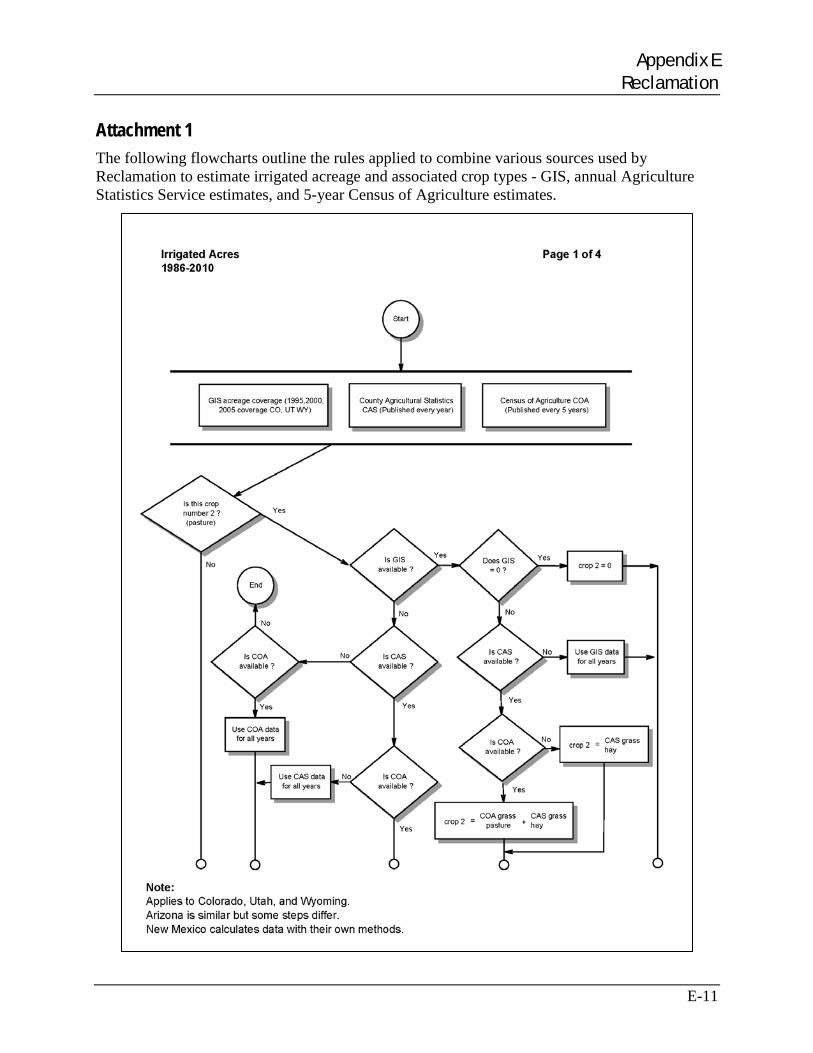
Appendix E Reclamation
E-11
Attachment 1 The following flowcharts outline the rules applied to combine various sources used by Reclamation to estimate irrigated acreage and associated crop types - GIS, annual Agriculture Statistics Service estimates, and 5-year Census of Agriculture estimates.
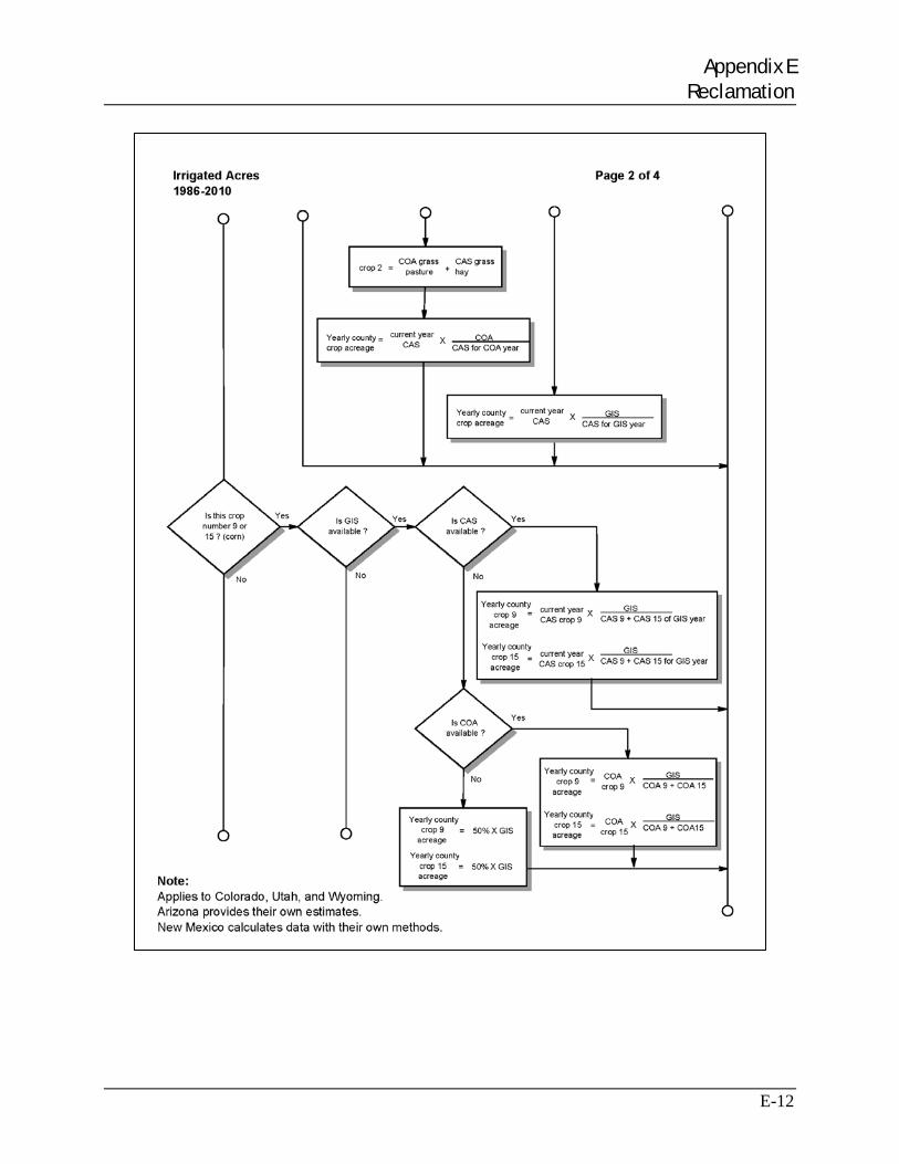
Appendix E Reclamation
E-12
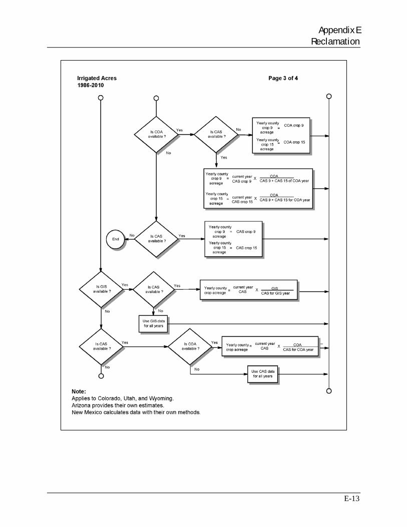
Appendix E Reclamation
E-13
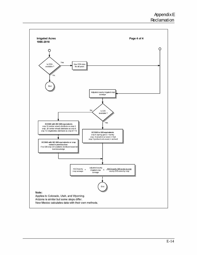
Appendix E Reclamation
E-14
Appendix F Upper Colorado River Basin Compact, 1948
Appendix F Upper Colorado River Basin Compact, 1948
F-1
Upper Colorado River Basin Compact, 1948
ARTICLE VI
The Commission shall determine the quantity of the consumptive use of water, which use is apportioned by Article III hereof, for the Upper Basin and for each State of the Upper Basin by the inflow outflow method in terms of man-made depletions of the virgin flow at Lee Ferry, unless the Commission, by unanimous action, shall adopt a different method of determination.
ARTICLE VIII (c) The Commission shall appoint a Secretary, who shall not be a member of the Commission, or an employee of any signatory State or of the United States of America while so acting. He shall serve for such term and receive such salary and perform such duties as the Commission may direct. The Commission may employ such engineering, legal, clerical and other personnel as, in its judgment, may be necessary for the performance of its functions under this Compact. In the hiring of employees, the Commission shall not be bound by the civil service laws of any State. (d) The Commission, so far as consistent with this Compact, shall have the power to: (1) Adopt rules and regulations; (2) Locate, establish, construct, abandon, operate and maintain water gaging stations; (3) Make estimates to forecast water run-off on the Colorado River and any of its tributaries; (4) Engage in cooperative studies of water supplies of the Colorado River and its tributaries; (5) Collect, analyze, correlate, preserve and report on data as to the stream flows, storage, diversions and use of the waters of the Colorado River, and any of its tributaries; (6) Make findings as to the quantity of water of the Upper Colorado River System used each year in the Upper Colorado River Basin and in each State thereof; (7) Make findings as to the quantity of water deliveries at Lee Ferry during each water year; (8) Make findings as to the necessity for and the extent of the curtailment of use, required, if any, pursuant to Article IV hereof; (9) Make findings to the quantity of reservoir losses and as to the share thereof chargeable under Article V hereof to each of the States; (10) Make findings of fact in the event of the occurrence of extraordinary drought or serious accident to the irrigation system in the Upper Basin, whereby deliveries by the Upper Basin of water which it may be required to deliver in order to aid in fulfilling obligations of the United States of America to the United Mexican States arising under the Treaty between the United States of America and the United Mexican States, dated February 3, 1944 (Treaty Series 994) become difficult, and report such findings to the Governors of the Upper Basin states, the President of the United States of America, the United States Section of the International Boundary and Water Commission, and such other Federal officials and agencies as it may deem appropriate to the end that the water allotted to Mexico under Division III of such treaty may be reduced in accordance with the terms of such Treaty; (11) Acquire and hold such personal and real property as may be necessary for the performance of its duties hereunder and to dispose of the same when no longer required; (12) Perform all functions required of it by this Compact and do all things necessary, proper or convenient in the performance of its duties hereunder, either independently or in cooperation with any state or federal agency;
Appendix F Upper Colorado River Basin Compact, 1948
F-2
(13) Make and transmit annually to the Governors of the signatory States and the President of the United States of America, with the estimated budget, a report covering the activities of the Commission for the preceding water year. (e) Except as otherwise provided in this Compact the concurrence of four members of the Commission shall be required in any action taken by it. (f) The Commission and its Secretary shall make available to the Governor of each of the signatory States any information within its possession at any time, and shall always provide free access to its records by the Governors of each of the States, or their representatives, or authorized representatives of the United States of America. (g) Findings of fact made by the Commission shall not be conclusive in any court, or before any agency or tribunal, but shall constitute prima facie evidence of the facts found. (h) The organization meeting of the Commission shall be held within four months from the effective date of Compact.
PUBLIC LAW 90-537
COLORADO RIVER BASIN PROJECT ACT
TITLE VI–GENERAL PROVISIONS: DEFINITIONS: CONDITIONS
SEC. 601. (a) Nothing in this Act shall be construed to alter, amend ,repeal, modify, or be in conflict with the provisions of the Colorado River Compact (45 Stat. 1057), the Upper Colorado River Basin Compact (63 Stat. 31), the Water Treaty of 1944 with the United Mexican States (Treaty Series 994; 59 Stat. 1219), the decree entered by the Supreme Court of the United States in Arizona against California and others (376 U.S. 340), or, except as otherwise provided herein, the Boulder Canyon Project Act (45 Stat. 1057), the Boulder Canyon Project Adjustment Act (54 Stat. 774; 43 U.S.C. 618a) or the Colorado River Storage Project Act (70 Stat. 105; 43 U.S.C. 620). (b) The Secretary is directed to– (1) make reports as to the annual consumptive uses and losses of water from the Colorado River system after each successive five year period, beginning with the five-year period starting on October 1, 1970. Such reports shall include a detailed breakdown of the beneficial consumptive use of water on a State-by-State basis. Specific figures on quantities consumptively used from the major tributary streams flowing into the Colorado River shall also be included on a State-by-State basis. Such reports shall be prepared in consultation with the States of the lower basin individually and with the Upper Colorado River Commission, and shall be transmitted to the President, the Congress, and to the Governors of each State signatory to the Colorado River Compact; and: (2) condition all contracts for the delivery of water originating in the drainage basin of the Colorado River system upon the availability of water under the Colorado River Compact.
Appendix F Upper Colorado River Basin Compact, 1948
F-3
(c) All Federal officers and agencies are directed to comply with the applicable provisions of this Act, and of the laws, treaty, compacts, and decree referred to in subsection (a) of this section, in the storage and release of water from all reservoirs and in the operation and maintenance of all facilities in the Colorado River system under the jurisdiction and supervision of the Secretary, and in the operation and maintenance of all works which may be authorized hereafter for the augmentation of the water supply of the Colorado River system. In the event of failure of any such officer or agency to so comply, any affected State may maintain an action to enforce the provisions of this section in the Supreme Court of the United States and consent is given to the joinder of the United States as a party in such suit or suits, as a defendant or otherwise.