asf mapready user manualasf mapready user manual 5 1. introduction this manual provides a complete...
TRANSCRIPT
ASF MapReady User Manual
Version 3.1
Alaska Satellite Facility Engineering Group

ASF MapReady User Manual
2
This page is intentionally blank
ASF MapReady User Manual
3
Table of Contents 1. Introduction ................................................................................................................ 5 2. General background .................................................................................................. 5
2.1 Data formats ..................................................................................................... 5 2.2 Calibration ........................................................................................................ 6 2.3 Terrain correction ............................................................................................. 7 2.4 Map projections .............................................................................................. 12 2.5 Polarization ..................................................................................................... 12 2.6 Configuration file ............................................................................................. 13 2.7 Temporary directories ..................................................................................... 13
3. Using the MapReady Graphical User Interface ........................................................ 14 3.1 Settings .......................................................................................................... 14
3.1.1 General ................................................................................................ 14 3.1.2 Calibration Tab ..................................................................................... 16 3.1.3 External Tab ......................................................................................... 17 3.1.4 Polarimetry Tab .................................................................................... 18 3.1.5 Terrain Correction Tab ......................................................................... 21 3.1.6 Geocode Tab ....................................................................................... 24 3.1.7 Export Tab ............................................................................................ 27
3.2 Input Files ....................................................................................................... 29 3.3 Completed Files.............................................................................................. 36 3.4 Summary Section ........................................................................................... 40
3.4.1 Footer buttons ...................................................................................... 40 3.4.2 Tool tips ................................................................................................ 41
3.5 Examples ........................................................................................................ 42 3.5.1 Converting optical ALOS AVNIR data into GeoTIFF format ................. 42 3.5.2 Converting optical ALOS PRISM data into GeoTIFF format ................. 46 3.5.3 Converting ALOS PALSAR data into GeoTIFF format ......................... 47 3.5.4 Terrain correcting standard beam RADARSAT imagery ...................... 51 3.5.5 Using the Cloude-Pottier Polarimetric decomposition .......................... 56 3.5.6 Correcting Palsar for Faraday Rotation ................................................ 60 3.5.7 Using Pauli decomposition with UAVSAR data .................................... 61
4. The interface between MapReady and PolSARPro ................................................. 63 5. ASF View ................................................................................................................. 66
5.1 Running ASF View ......................................................................................... 66 5.2 Using ASF View.............................................................................................. 66
5.2.1 Basic Mouse Usage ............................................................................. 67 5.2.2 Defining Polygons ................................................................................ 68 5.2.3 Other Useful Keyboard Commands...................................................... 70
5.3 Saving Image Subsets .................................................................................... 71 5.4 Toolbar Buttons .............................................................................................. 74 5.5 Information Tabs ............................................................................................. 75
6. The Projection Coordinate Converter ....................................................................... 79 7. Using MapReady from the command line (asf_mapready) ...................................... 80
7.1 Generating a configuration file ........................................................................ 80
ASF MapReady User Manual
4
7.2 Import ............................................................................................................. 86 7.3 Polarimetry ..................................................................................................... 87 7.4 Terrain correction ........................................................................................... 87 7.5 Geocoding ...................................................................................................... 89 7.6 Export ............................................................................................................. 90 7.7 Default values file ........................................................................................... 91 7.8 MapReady settings file ................................................................................... 93 7.9 Running asf_mapready in batch mode ........................................................... 94
8. Overview of other command line tools of the MapReady suite ................................ 95 adjust_bands ........................................................................................................... 95 analyze_yaw ............................................................................................................ 95 asf_calibrate ............................................................................................................ 95 asf_calpol ................................................................................................................. 96 asf_export ................................................................................................................ 97 asf_geocode ............................................................................................................ 98 asf_import ................................................................................................................ 98 asf_kml_overlay ....................................................................................................... 99 asf_mapready .......................................................................................................... 99 asf_proj2proj ............................................................................................................ 99 asf_terrcorr ............................................................................................................ 100 asf_view ................................................................................................................. 100 brs2jpg ................................................................................................................... 100 combine ................................................................................................................. 100 deskew ................................................................................................................... 100 diffimage ................................................................................................................ 101 diffmeta .................................................................................................................. 101 farcorr .................................................................................................................... 101 fftMatch .................................................................................................................. 101 fill_holes ................................................................................................................. 101 flip .......................................................................................................................... 102 geoid_adjust .......................................................................................................... 102 meta2envi .............................................................................................................. 102 metadata ................................................................................................................ 102 mosaic ................................................................................................................... 102 refine_geolocation .................................................................................................. 103 resample ................................................................................................................ 103 shift_geolocation .................................................................................................... 103 smooth ................................................................................................................... 104 sr2gr ....................................................................................................................... 104 to_sr ....................................................................................................................... 104 trim ......................................................................................................................... 104 write_ppf ................................................................................................................ 104
9. Handling multi-band files with the command line tools ........................................... 106 Appendix A – Configuration File Example .................................................................. 107 Appendix B – MapReady functionality ......................................................................... 117

ASF MapReady User Manual
5
1. Introduction This manual provides a complete overview of the conversion from operationally produced synthetic aperture radar (SAR) and optical data to a variety of user friendly formats ready for additional processing, viewing, or being utilized in GIS software. It presents the theoretical background for the formats, corrections and processing steps in the processing flow. This manual describes the functionality of the graphical user interface (GUI) and command line interface tools provided in the MapReady remote sensing software package. Examples of completed runs are provided. A number of exercises are provided explain how the MapReady software can be utilized for a variety of different applications. This software and documentation was produced by the Engineering group at the Alaska Satellite Facility, part of the Geophysical Institute at the University of Alaska Fairbanks.
2. General background This section provides some background information to allow the user to make the most effective use of the MapReady software.
2.1 Data formats After processing the analog SAR signal to binary SAR signal data, the data is called level zero (L0) data in SKY telemetry format (STF). The level zero data covers a certain area on the ground in the form of a swath. The length of the swath depends on the amount of data originally collected during the actual acquisition. The size of the files varies but can easily be as large as a few gigabytes. The level zero swaths are then subdivided in frames. For ERS imagery, these frames have a size of 100 by 100 kilometers, which is equivalent to about 26000 lines of radar data. The accompanying leader file is defined in CEOS standard format. This is why these data sets are referred to as CEOS frames. The CEOS data come in three different flavors. The CEOS level zero data is raw signal data that needs to run through a SAR processor before it can be visualized. The result of the SAR processing, CEOS single look complex (SLC) level one (L1) data, is primarily used for SAR interferometry, as it contains both amplitude and the required phase information. Furthermore, the data has not been multilooked at this point, i.e. the pixels are not yet square (with the exception of RADARSAT-1 fine beam data). To be useful for SAR interferometry, the data generally needs to be deskewed during the SAR processing. The resulting so-called zero Doppler geometry ensures that two interferometric data sets can be combined without introducing any further distortions. In order to be visualized the data needs to be first converted from its complex form into an amplitude image. CEOS level one data (L1) is the most commonly used format. It does not require any further processing to be useful for regular use.
ASF MapReady User Manual
6
After ingesting the data, all files are stored in an Alaska Satellite Facility (ASF) Internal format. In this format, the image files are flat generic binary files without any headers and have the extension .img. Associated with each .img file is a human-readable (text) metadata file. The metadata files have a .meta file extension.
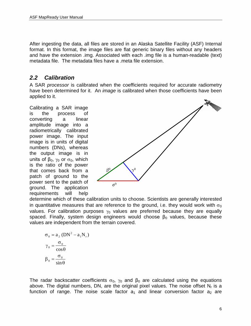
2.2 Calibration A SAR processor is calibrated when the coefficients required for accurate radiometry have been determined for it. An image is calibrated when those coefficients have been applied to it. Calibrating a SAR image is the process of converting a linear amplitude image into a radiometrically calibrated power image. The input image is in units of digital numbers (DNs), whereas the output image is in units of β0, γ0 or σ0, which is the ratio of the power that comes back from a patch of ground to the power sent to the patch of ground. The application requirements will help determine which of these calibration units to choose. Scientists are generally interested in quantitative measures that are reference to the ground, i.e. they would work with σ0 values. For calibration purposes γ0 values are preferred because they are equally spaced. Finally, system design engineers would choose β0 values, because these values are independent from the terrain covered.
θσ
=β
θσ
=γ
−=σ
sin
cos
)Na(DN a
00
00
r12
20
The radar backscatter coefficients σ0, γ0 and β0 are calculated using the equations above. The digital numbers, DN, are the original pixel values. The noise offset Nr is a function of range. The noise scale factor a1 and linear conversion factor a2 are
ASF MapReady User Manual
7
determined during the calibration of the processor. The values resulting from the equations above are in power scale. In order to convert them into dB values the following relationship is utilized:
scale) power(log10dB 10⋅=
Calibrated images generally use the logarithmic dB scale. When image statistics are calculated for calibrated imagery, special attention needs to be given to the logarithmic nature of the values. In order to correctly determine the mean value of any part of the image, for example, the calculation has to be based on power scale values. The mean power scale value can then be converted back into the logarithmic scale to correctly represent dB values.
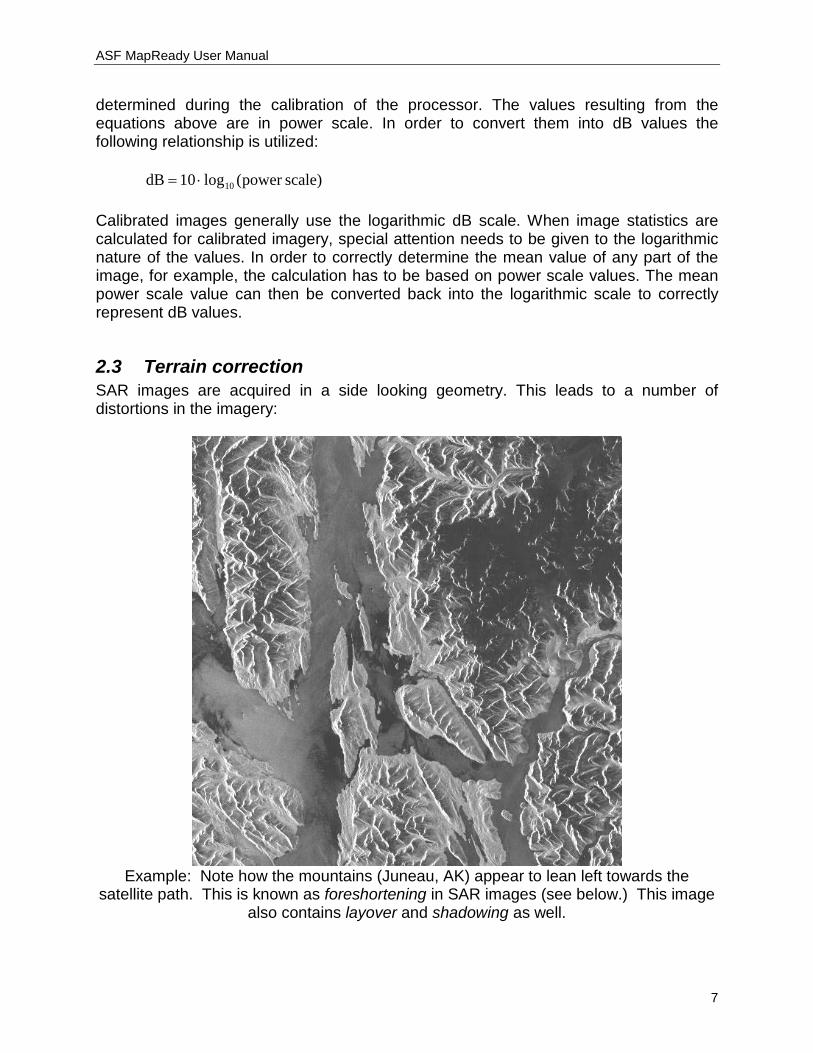
2.3 Terrain correction SAR images are acquired in a side looking geometry. This leads to a number of distortions in the imagery:
Example: Note how the mountains (Juneau, AK) appear to lean left towards the
satellite path. This is known as foreshortening in SAR images (see below.) This image also contains layover and shadowing as well.
ASF MapReady User Manual
8
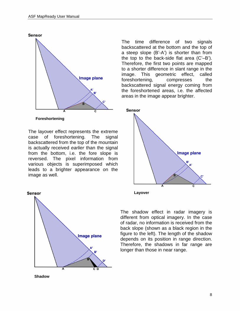
The time difference of two signals backscattered at the bottom and the top of a steep slope (B’-A’) is shorter than from the top to the back-side flat area (C’–B’). Therefore, the first two points are mapped to a shorter difference in slant range in the image. This geometric effect, called foreshortening, compresses the backscattered signal energy coming from the foreshortened areas, i.e. the affected areas in the image appear brighter.
The layover effect represents the extreme case of foreshortening. The signal backscattered from the top of the mountain is actually received earlier than the signal from the bottom, i.e. the fore slope is reversed. The pixel information from various objects is superimposed which leads to a brighter appearance on the image as well.
The shadow effect in radar imagery is different from optical imagery. In the case of radar, no information is received from the back slope (shown as a black region in the figure to the left). The length of the shadow depends on its position in range direction. Therefore, the shadows in far range are longer than those in near range.
Foreshortening
Shadow
Layover
ASF MapReady User Manual
9
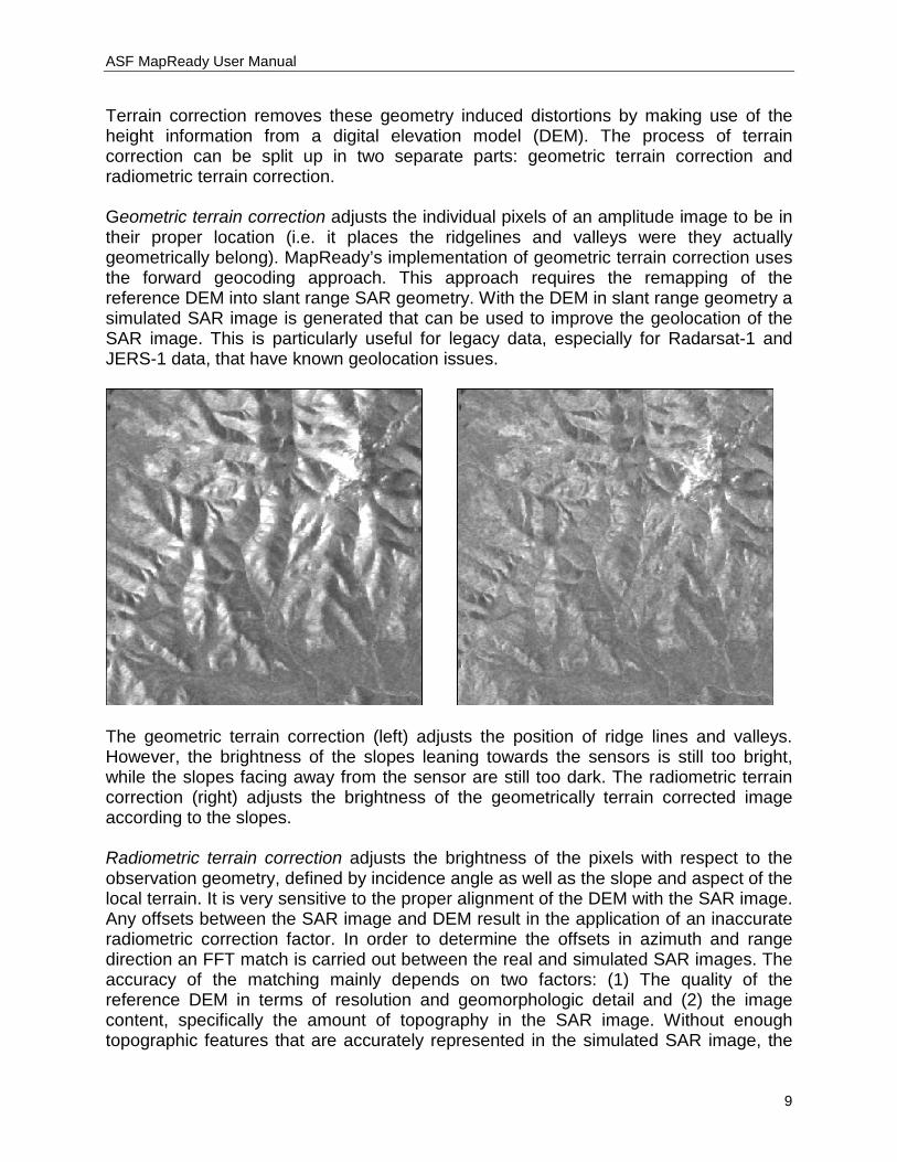
Terrain correction removes these geometry induced distortions by making use of the height information from a digital elevation model (DEM). The process of terrain correction can be split up in two separate parts: geometric terrain correction and radiometric terrain correction. Geometric terrain correction adjusts the individual pixels of an amplitude image to be in their proper location (i.e. it places the ridgelines and valleys were they actually geometrically belong). MapReady’s implementation of geometric terrain correction uses the forward geocoding approach. This approach requires the remapping of the reference DEM into slant range SAR geometry. With the DEM in slant range geometry a simulated SAR image is generated that can be used to improve the geolocation of the SAR image. This is particularly useful for legacy data, especially for Radarsat-1 and JERS-1 data, that have known geolocation issues.
The geometric terrain correction (left) adjusts the position of ridge lines and valleys. However, the brightness of the slopes leaning towards the sensors is still too bright, while the slopes facing away from the sensor are still too dark. The radiometric terrain correction (right) adjusts the brightness of the geometrically terrain corrected image according to the slopes. Radiometric terrain correction adjusts the brightness of the pixels with respect to the observation geometry, defined by incidence angle as well as the slope and aspect of the local terrain. It is very sensitive to the proper alignment of the DEM with the SAR image. Any offsets between the SAR image and DEM result in the application of an inaccurate radiometric correction factor. In order to determine the offsets in azimuth and range direction an FFT match is carried out between the real and simulated SAR images. The accuracy of the matching mainly depends on two factors: (1) The quality of the reference DEM in terms of resolution and geomorphologic detail and (2) the image content, specifically the amount of topography in the SAR image. Without enough topographic features that are accurately represented in the simulated SAR image, the
ASF MapReady User Manual
10
results of the matching are poor. Erroneous offsets from bad matches are more difficult to notice than actual matching failures.
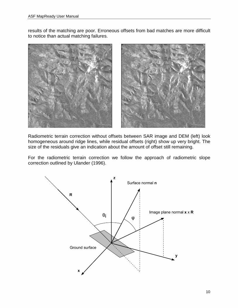
Radiometric terrain correction without offsets between SAR image and DEM (left) look homogeneous around ridge lines, while residual offsets (right) show up very bright. The size of the residuals give an indication about the amount of offset still remaining. For the radiometric terrain correction we follow the approach of radiometric slope correction outlined by Ulander (1996).

ASF MapReady User Manual
11
Three-dimensional geometry of ground surface and its projection into the SAR image. x and R are azimuth and slant range coordinates, n is the surface normal, φ is the projection angle, and θi is the local incidence angle (after Ulander, 1996).
The Ulander approach uses the surface normal and, therefore, the image plane normal is rotationally symmetric. This leads to a complete independence from the aspect of the slope for any given pixel. The equation for this radiometric correction, applied to sigma values in power scale is the following:
with φ the projection angle between surface normal and image plane normal and θi the local incidence angle. The radiometric terrain correction is entirely done using amplitude images to avoid any special cases in the processing flow with respect to radiometry. This requires the conversion of the radiometric correction factor from σ0 to amplitude. For the ALOS Palsar calibration scheme, for example, this works as follows. The calibration equation to generate power scale in sigma radiometry is
with the calibration factor cf and the amplitude digital numbers DN. The resulting equation for the radiometrically corrected amplitude DNrad values is
This approach ensures that values in any radiometry can be calculated by simply applying the respective calibration equation. Ulander, L.M.H., 1996. Radiometric slope correction of synthetic-aperture radar images.
IEEE Transactions on Geoscience and Remote Sensing, 34(5): 1115 – 1122.

ASF MapReady User Manual
12
2.4 Map projections Maps are a two-dimensional representation of the three-dimensional real world. Projecting three-dimensional coordinates into a two-dimensional space is not possible without distortions in feature shape, area, distance, or direction. A very practical illustration of this problem is to lay a carefully peeled orange onto a flat table surface without fracturing it. Map projections can preserve some of the above mentioned characteristics at a time, but never all of them. Selecting an appropriate map projection allows them to be suitable for certain applications and/or geographical regions. Cylindrical projections work best in equatorial areas. The Universal Transverse Mercator (UTM) projection is the most commonly used one from this family of map projections. The distortions within the UTM projection are manageable as long as the projected area is not very large. Conic projections, commonly defined with two standard parallels, are often used in the mid-latitude regions. In this case, the Albers Conic Equal Area projection preserves area, while the Lambert Conformal Conic projection preserves angles. Azimuthal projections are mostly used in the Polar Regions. The Polar Stereographic projection and Lambert Azimuth Equal Area projection are well known representatives of this type of projection. The ASF MapReady software currently supports five of the most commonly used map projections: • Universal Transverse Mercator (UTM) • Albers Conical Equal Area • Polar Stereographic • Lambert Conformal Conic • Lambert Azimuthal Equal Area
2.5 Polarization ALOS/PALSAR data can be obtained which uses multiple polarizations to image a scene, including dual-pol (two different polarizations) and quad-pol (four different polarizations). The term polarization refers to the orientation of the electric (E-field) vector in the electromagnetic wave (signal) emitted by conventional radar systems. SAR satellites generally transmit in either a vertical (perpendicular to the earth’s surface) or a horizontal (parallel with the earth’s surface) polarization, and then receive in either a vertical or horizontal orientation or both. Other orientations such as at other vector angles and elliptical or circular polarizations are generally not available from remote sensing platforms. The ALOS/PALSAR satellite, for example, can transmit either horizontally (H) or vertically (V) polarized waves, and receive either as well. The two-letter polarization field of the ASF metadata is always one of HH, HV, VH or VV; the first

ASF MapReady User Manual
13
letter refers to which polarization was transmitted and the second is which was received. For example, if H is transmitted, and V is received (HV), we’re looking at how the scatterers on the ground changed the polarization of the wave from horizontal to vertical. The RADARSAT-1 and ERS-1/2 satellites transmitted and received only a single polarization; RADARSAT-1 always sent and received horizontally polarized waves (HH), ERS-1 and ERS-2 always sent and received vertically polarized waves (VV.) ALOS/PALSAR quad-pol data contains all four combinations – the satellite alternates between the four, yielding more information about what is on the ground, since various terrain features respond differently to each polarization. Note that in trade for this additional information, due to bandwidth and storage limitations on the platform (satellite), that dual-pol and quad-pol products generally have lower resolution than single-pol products.
2.6 Configuration file The MapReady tool has a large number of options and parameters that define the exact processing flow to be run. In order to keep track of the parameters in an organized fashion, they are stored in a configuration file. The graphical user interface version of the tool produces this configuration file from user-selected settings on the fly and then executes all of the selected processing steps based on that file. For simplicity’s sake, the configuration file produced by the graphical user interface is of the same type as the one required to run the command line tool. For throughput reasons, a batch mode is available that allows users to run large quantities of data files through the system with minimal user input. All essential options can be stored in a default values file that is used to process all files in the batch file list using the same set of parameters (other than the input and output file names.) The defaults settings file is in addition to the configuration file. Setting these files up for use with the command line tool is described later in the "Running asf_mapready in batch mode" section, and this section should be understood clearly before using the default settings file so you understand which overrides the other.
2.7 Temporary directories MapReady provides the user with the capability of keeping intermediate results for further analysis, e.g. errors, warnings, and results of each processing step. During each run, these intermediate files are kept in separate subdirectories for each data set. In order to ensure that intermediate results are not accidentally overwritten by consecutive processing of the same input files, the names of the subdirectories are created with a new date and time stamp. The intermediate files themselves have descriptive names that should make it easy to identify the files for further analysis.

ASF MapReady User Manual
14
3. Using the MapReady Graphical User Interface The graphical user interface (GUI) of the MapReady package provides the user with a convenient and interactive way to convert SAR data from their specific CEOS or STF format, explained in detail in the background section, into more user friendly formats that the majority of software packages dealing with images and their processing and analysis are able to handle. As part of the conversion process, the user can perform a number of modifications that make SAR data more powerful to use. These modifications include • Converting the digital numbers of an image into radiometrically calibrated values; • Converting the image from its SAR geometry into a map projection, i.e. geocoding it; • Correcting the SAR image for its geometric distortions using a digital elevation
model, i.e. terrain correcting it. • Extracting polarimetric classifications from it • Converting it into various graphical file formats The GUI consists of six areas (tabs) that allow the user to set up, monitor and execute the conversion processing flow. The functionality of these six areas is described in this section of the manual in more detail.
The "Settings" section, and the two "Files" sections contain expand/collapse buttons, which hide and show each section.
3.1 Settings This area consists of one general and six processing tabs that define all the parameters used in the conversion process, seven tabs in all (generally clicked and options set in left to right order.)
3.1.1 General The General tab controls which of the six processing steps take place: Importing, Polarimetry, Terrain Correction, Geocoding, and Exporting. There is one additional tab located between Import Settings and Polarimetry to allow running a ‘plug in’ tool after import but before other processing. The Import processing step is required and therefore cannot be deselected; however the other steps are optional. By default, only Import and Export are turned on. Checking/unchecking each step’s checkbox will turn on or off the tab that contains the
ASF MapReady User Manual
15
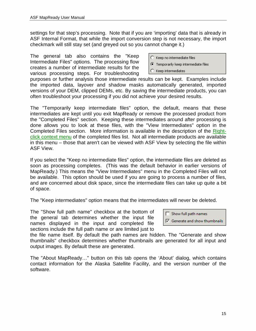
settings for that step’s processing. Note that if you are ‘importing’ data that is already in ASF Internal Format, that while the import conversion step is not necessary, the import checkmark will still stay set (and greyed out so you cannot change it.) The general tab also contains the "Keep Intermediate Files" options. The processing flow creates a number of intermediate results for the various processing steps. For troubleshooting purposes or further analysis those intermediate results can be kept. Examples include the imported data, layover and shadow masks automatically generated, imported versions of your DEM, clipped DEMs, etc. By saving the intermediate products, you can often troubleshoot your processing if you did not achieve your desired results. The "Temporarily keep intermediate files" option, the default, means that these intermediates are kept until you exit MapReady or remove the processed product from the "Completed Files" section. Keeping these intermediates around after processing is done allows you to look at these files, with the "View Intermediates" option in the Completed Files section. More information is available in the description of the Right-click context menu of the completed files list. Not all intermediate products are available in this menu – those that aren't can be viewed with ASF View by selecting the file within ASF View. If you select the "Keep no intermediate files" option, the intermediate files are deleted as soon as processing completes. (This was the default behavior in earlier versions of MapReady.) This means the "View Intermediates" menu in the Completed Files will not be available. This option should be used if you are going to process a number of files, and are concerned about disk space, since the intermediate files can take up quite a bit of space. The "Keep intermediates" option means that the intermediates will never be deleted. The "Show full path name" checkbox at the bottom of the general tab determines whether the input file names displayed in the input and completed file sections include the full path name or are limited just to the file name itself. By default the path names are hidden. The "Generate and show thumbnails" checkbox determines whether thumbnails are generated for all input and output images. By default these are generated. The "About MapReady…" button on this tab opens the ‘About’ dialog, which contains contact information for the Alaska Satellite Facility, and the version number of the software.
ASF MapReady User Manual
16
3.1.2 Calibration Tab Note that all processing other than the import step requires the data to be in the ASF Internal Format file format. This is in fact what the import step accomplishes (additionally applying the selected radiometric calibration). The result of each processing step (other than export) will be another set of data in ASF Internal Format. Only export will change the file format to something else, i.e. to a graphics file format for GIS and viewer software compatibility. ASF Internal Format data is a set of two files, one that contains metadata (information) about the data in the dataset and another that contains the data itself in binary format. The files share the same name but have different file extensions. The metadata file ends in ".meta" and the data file ends in ".img". SAR data in its detected form reflects the intensity or amplitude of the reflected backscatter. In order to use SAR data in a quantitative fashion, it is advisable to radiometrically correct the data.
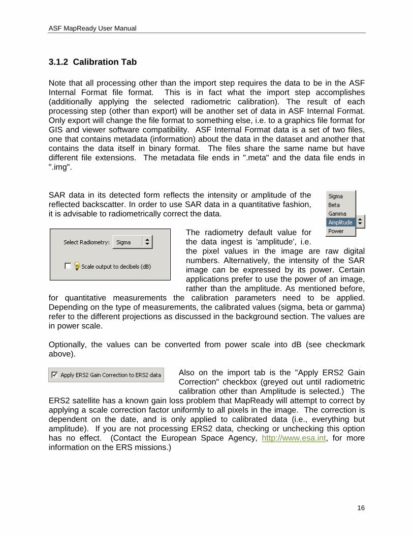
The radiometry default value for the data ingest is 'amplitude', i.e. the pixel values in the image are raw digital numbers. Alternatively, the intensity of the SAR image can be expressed by its power. Certain applications prefer to use the power of an image, rather than the amplitude. As mentioned before,
for quantitative measurements the calibration parameters need to be applied. Depending on the type of measurements, the calibrated values (sigma, beta or gamma) refer to the different projections as discussed in the background section. The values are in power scale. Optionally, the values can be converted from power scale into dB (see checkmark above).
Also on the import tab is the "Apply ERS2 Gain Correction" checkbox (greyed out until radiometric calibration other than Amplitude is selected.) The
ERS2 satellite has a known gain loss problem that MapReady will attempt to correct by applying a scale correction factor uniformly to all pixels in the image. The correction is dependent on the date, and is only applied to calibrated data (i.e., everything but amplitude). If you are not processing ERS2 data, checking or unchecking this option has no effect. (Contact the European Space Agency, http://www.esa.int, for more information on the ERS missions.)
ASF MapReady User Manual
17
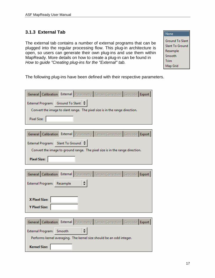
3.1.3 External Tab The external tab contains a number of external programs that can be plugged into the regular processing flow. This plug-in architecture is open, so users can generate their own plug-ins and use them within MapReady. More details on how to create a plug-in can be found in How to guide "Creating plug-ins for the "External" tab. The following plug-ins have been defined with their respective parameters.

ASF MapReady User Manual
18
3.1.4 Polarimetry Tab When processing complex quad-pol data (PALSAR Level 1.1), several different visualizations are available. These polarimetric Decompositions take the four different bands of complex data (HH, HV, VH and VV) and mathematically combine them to produce three bands of real-valued data, which can be directly mapped to RGB and displayed. The mappings attempt to highlight the ways in which the various terrain features respond to the polarized signal data from the satellite.
When the Polarimetry tab is active, the Export tab's RGB options changes to "Export RGB Image according to Polarimetric selection". This means that the RGB channels in
ASF MapReady User Manual
19
the final result are determined by the polarimetric decomposition. The channels and how they are calculated from the input quad-pol data are listed next to the radio button on the Polarimetry tab. For example, for Pauli the red channel is calculated by subtracting the complex VV-band value from the complex HH-band value, and then determining the magnitude of the resulting complex value. All of the polarimetric decompositions require SLC data (except Sinclair). The polarimetric calculations will multilook the data, since many of the calculations require that the data be ensemble averaged; MapReady performs the ensemble averaging using the multilooking window. For ALOS/PALSAR, this means we are using an 8x1 ensemble average, but no smoothing occurs – each pixel is only used once and the output has 1/8 the number of lines as the input, and the same number of samples. The Pauli Decomposition The Pauli Decomposition is calculated from the input data using the following formulas:
• Red: |HH-VV| — even bounce • Green: |HV+VH| — rotated dihedral • Blue: |HH+VV| — odd bounce
Using the Pauli decomposition to visualize the data allows one to see the dominant scattering mechanisms in different areas of the scene. For example, areas with buildings (where the even bounce return will dominate) will look reddish. The Sinclair Decomposition The Sinclair Decomposition is a simple decomposition that combines all four polarizations into a single RGB image in a simple way that doesn't require complex data. The green channel is the average of the cross-polarization terms, which theoretically are equal but may not be due to noise, etc. This means that the Sinclair decomposition doesn’t require SLC data, it can be done with Level 1.5 quad-pol data; whereas the other decompositions require SLC data (Level 1.1). Polarimetric decompositions added to MapReady in future versions will likely require SLC data as well. Cloude-Pottier Classification The Cloude-Pottier classification scheme produces output with the data categorized into either 8 or 16 classes. The classification is based on three parameters which can be calculated from the 4-band complex data at each pixel. These parameters are calculated from the coherence matrix, which is calculated for each pixel. These parameters are entropy, anisotropy, and alpha.
ASF MapReady User Manual
20
Entropy is an indication of the degree of randomness in the scattering process. Low entropy means there is a single dominant scattering mechanism in that pixel; high entropy means multiple scattering mechanisms are present in the pixel. Anisotropy represents the relative importance of the non-dominant scatterers. When entropy is low, the anisotropy parameter means very little, but for high entropy it is a useful indication of the strength of the secondary scatters. Alpha can be used to identify what type of scatterer is the dominant one. When alpha is close to 0, single-bounce scattering (e.g., a rough surface) is dominant. For alpha near 90°, the dominant scatterer is double-bounce. Alphas in between these extremes represent a combination of both; at 45° we have equal amounts of both which usually corresponds to volume scattering. The Cloude-Pottier parameters can be obtained directly (skipping the classification) by selecting the "Entropy, Anisotropy, Alpha" option. This is the only option where you may assign RGB channels yourself, or choose to export three separate grayscale images (one for each of entropy, anisotropy, and alpha); with the other polarimetric decompositions the RGB channel assignment is determined by the decomposition. Some of the intermediate files generated for the Cloude-Pottier Decomposition are useful, and are described in the Examples, below. For more information on the Cloude-Pottier decomposition: Cloude, S.R. and Pottier, E., 1997. An Entropy Based Classification Scheme for Land
Applications of Polarimetric SAR. IEEE Transactions on Geoscience and Remote Sensing, 35(1):68-78.
Freeman-Durden The Freeman-Durden decomposition is a model-based approach – it attempts to fit the combination of three simple scattering mechanisms to the polarimetric data. These mechanisms are (i) even- or double-bounce scatter from a pair of orthogonal surfaces with different dielectric constants, (ii) canopy scatter from a cloud of randomly oriented dipoles, and (iii) Bragg scatter from a moderately rough surface. These three components are assigned to the three color channels during export: the double-bounce component (i) is assigned to the Red channel, the canopy component (ii) is assigned to the Green channel, and the rough surface component (iii) is assigned to the Blue channel. The results look similar to the Pauli decomposition. For more information on the Freeman-Durden decomposition:
ASF MapReady User Manual
21
Freeman, A. and Durden, S., 1998. A Three-Component Scattering Model for
Polarimetric SAR Data. IEEE Transactions on Geoscience and Remote Sensing, 36(3):963-973.
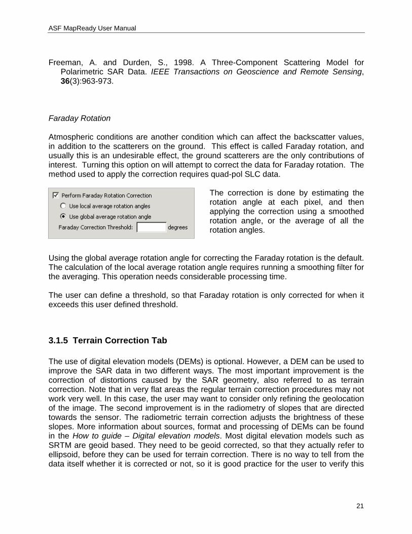
Faraday Rotation Atmospheric conditions are another condition which can affect the backscatter values, in addition to the scatterers on the ground. This effect is called Faraday rotation, and usually this is an undesirable effect, the ground scatterers are the only contributions of interest. Turning this option on will attempt to correct the data for Faraday rotation. The method used to apply the correction requires quad-pol SLC data.
The correction is done by estimating the rotation angle at each pixel, and then applying the correction using a smoothed rotation angle, or the average of all the rotation angles.
Using the global average rotation angle for correcting the Faraday rotation is the default. The calculation of the local average rotation angle requires running a smoothing filter for the averaging. This operation needs considerable processing time. The user can define a threshold, so that Faraday rotation is only corrected for when it exceeds this user defined threshold.
3.1.5 Terrain Correction Tab The use of digital elevation models (DEMs) is optional. However, a DEM can be used to improve the SAR data in two different ways. The most important improvement is the correction of distortions caused by the SAR geometry, also referred to as terrain correction. Note that in very flat areas the regular terrain correction procedures may not work very well. In this case, the user may want to consider only refining the geolocation of the image. The second improvement is in the radiometry of slopes that are directed towards the sensor. The radiometric terrain correction adjusts the brightness of these slopes. More information about sources, format and processing of DEMs can be found in the How to guide – Digital elevation models. Most digital elevation models such as SRTM are geoid based. They need to be geoid corrected, so that they actually refer to ellipsoid, before they can be used for terrain correction. There is no way to tell from the data itself whether it is corrected or not, so it is good practice for the user to verify this

ASF MapReady User Manual
22
detail of the DEM before using. The correction is applied by default in the GUI, but can also be applied using the command line tool geoid_adjust.
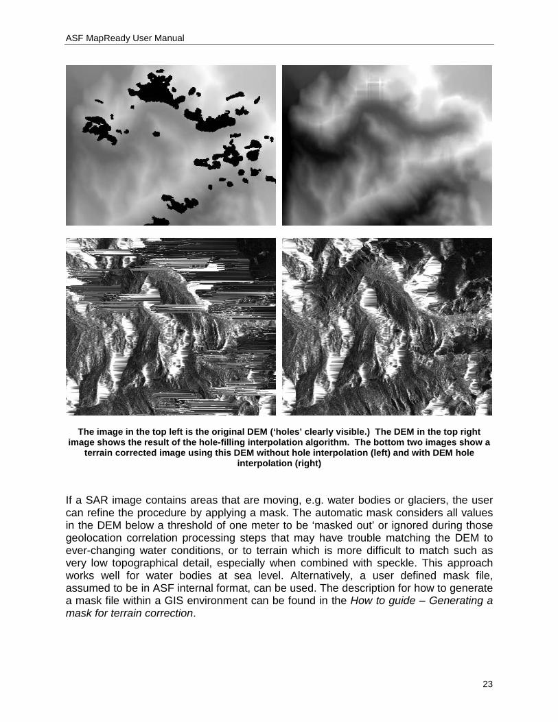
Once a DEM is defined in MapReady, by default the geolocation of the input SAR image is refined by the DEM. However, the user has a number of DEM and terrain correction related options to choose from. Some DEMs contain small ‘holes’ or regions of no data that appear as black specks or small blank spots. The data that is missing in these spots will generally result in minor defects showing up in the final product. If you so choose, you can opt to “Fill DEM holes with interpolated values” to smoothly interpolate the terrain over the regions with missing data. While this will prevent minor defects from occluding the terrain surrounding the DEM holes, the trade off is that the terrain that exists within the holes is now a best-estimate. It is suggested if your DEM contains holes that you try the processing with the interpolation algorithm turned on and off then compare the results to help you decide which method results in least impact for your purposes.
ASF MapReady User Manual
23
The image in the top left is the original DEM (‘holes’ clearly visible.) The DEM in the top right image shows the result of the hole-filling interpolation algorithm. The bottom two images show a
terrain corrected image using this DEM without hole interpolation (left) and with DEM hole interpolation (right)
If a SAR image contains areas that are moving, e.g. water bodies or glaciers, the user can refine the procedure by applying a mask. The automatic mask considers all values in the DEM below a threshold of one meter to be ‘masked out’ or ignored during those geolocation correlation processing steps that may have trouble matching the DEM to ever-changing water conditions, or to terrain which is more difficult to match such as very low topographical detail, especially when combined with speckle. This approach works well for water bodies at sea level. Alternatively, a user defined mask file, assumed to be in ASF internal format, can be used. The description for how to generate a mask file within a GIS environment can be found in the How to guide – Generating a mask for terrain correction.
ASF MapReady User Manual
24
The accuracy of the data geolocation mainly depends on the quality of the orbit information. Some legacy data have issues, in case of JERS data pretty severe issues, with that while confidence in the geolocation for data from more recently launched satellites such ALOS Palsar is generally high. In order to improve the geolocation of the processed data, we can use a matching technique based on Fast Fourier Transforms (FFTs). For this step a simulated SAR image is derived from the DEM and matched with the real image used in the processed. The FFT matching is used to determine the offsets in azimuth and range. These offsets are then iteratively applied until the solution converges to offsets within one pixel in both directions. Currently, the FFT matching for ALOS Palsar level 1.1 data is entirely switched off. Furthermore, the results for low relief areas should be taken with caution. With limited topography around the simulated SAR image lacks features that the algorithm is able to match. The number of matches with low confidence levels that even decrease the geolocation accuracy significantly increases in flat areas. The selection of FFT matching should be carefully evaluated and done on a case by case basis. The terrain correction itself is always a function of the quality of the DEM used for the correction. The terrain correction corrects the distortions in the SAR image using the height information in the DEM. The terrain correction is performed using the original pixel of the input data. This behavior can be overridden by specifying the otherwise optional pixel size. The pixel size option in the Geocoding tab (described below) is more appropriate if you are attempting to size the final image product, the pixel size value specified here should be selected based on the pixel size of the DEM. Apart from the geometric correction performed by the terrain correction, the image can be also corrected for its radiometry. The correction adjusts the brightness of the slopes facing the sensor during the acquisition. For more details refer to the terrain correction section. By default layover and shadow regions in the terrain corrected image are filled with interpolated values. By deselecting this option, the algorithm fills these data holes with zeros. The layover/shadow masks as well as the clipped DEM, both generated in the terrain correction process, can be saved for further analysis. These products are very specific to this process and do not fall into the general scheme of keeping intermediate products, if selected. More information about the layover/shadow mask is available in the Examples section, below.
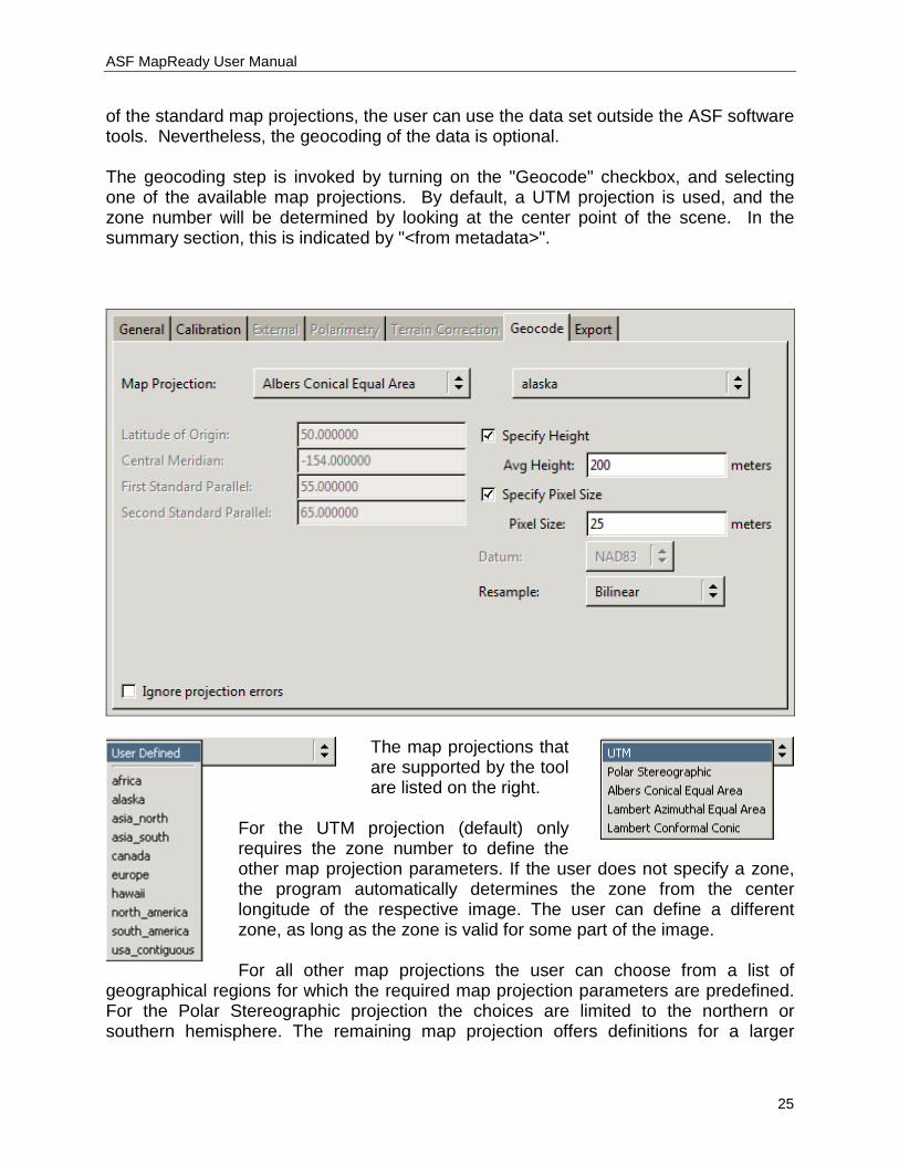
3.1.6 Geocode Tab The geocoding step is an essential step to establish the relation from the SAR image geometry to the real world. By transforming the image from the SAR geometry into one
ASF MapReady User Manual
25
of the standard map projections, the user can use the data set outside the ASF software tools. Nevertheless, the geocoding of the data is optional. The geocoding step is invoked by turning on the "Geocode" checkbox, and selecting one of the available map projections. By default, a UTM projection is used, and the zone number will be determined by looking at the center point of the scene. In the summary section, this is indicated by "<from metadata>".
The map projections that are supported by the tool are listed on the right.
For the UTM projection (default) only requires the zone number to define the other map projection parameters. If the user does not specify a zone, the program automatically determines the zone from the center longitude of the respective image. The user can define a different zone, as long as the zone is valid for some part of the image. For all other map projections the user can choose from a list of
geographical regions for which the required map projection parameters are predefined. For the Polar Stereographic projection the choices are limited to the northern or southern hemisphere. The remaining map projection offers definitions for a larger
ASF MapReady User Manual
26
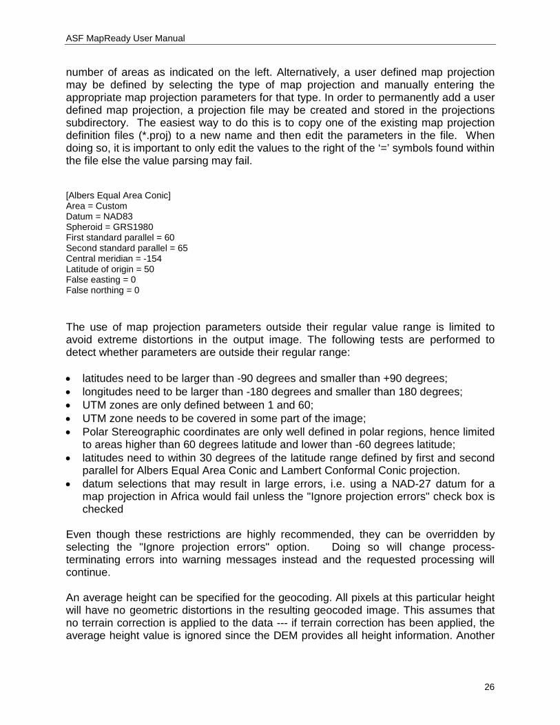
number of areas as indicated on the left. Alternatively, a user defined map projection may be defined by selecting the type of map projection and manually entering the appropriate map projection parameters for that type. In order to permanently add a user defined map projection, a projection file may be created and stored in the projections subdirectory. The easiest way to do this is to copy one of the existing map projection definition files (*.proj) to a new name and then edit the parameters in the file. When doing so, it is important to only edit the values to the right of the ‘=’ symbols found within the file else the value parsing may fail.
[Albers Equal Area Conic] Area = Custom Datum = NAD83 Spheroid = GRS1980 First standard parallel = 60 Second standard parallel = 65 Central meridian = -154 Latitude of origin = 50 False easting = 0 False northing = 0 The use of map projection parameters outside their regular value range is limited to avoid extreme distortions in the output image. The following tests are performed to detect whether parameters are outside their regular range: • latitudes need to be larger than -90 degrees and smaller than +90 degrees; • longitudes need to be larger than -180 degrees and smaller than 180 degrees; • UTM zones are only defined between 1 and 60; • UTM zone needs to be covered in some part of the image; • Polar Stereographic coordinates are only well defined in polar regions, hence limited
to areas higher than 60 degrees latitude and lower than -60 degrees latitude; • latitudes need to within 30 degrees of the latitude range defined by first and second
parallel for Albers Equal Area Conic and Lambert Conformal Conic projection. • datum selections that may result in large errors, i.e. using a NAD-27 datum for a
map projection in Africa would fail unless the "Ignore projection errors" check box is checked
Even though these restrictions are highly recommended, they can be overridden by selecting the "Ignore projection errors" option. Doing so will change process-terminating errors into warning messages instead and the requested processing will continue. An average height can be specified for the geocoding. All pixels at this particular height will have no geometric distortions in the resulting geocoded image. This assumes that no terrain correction is applied to the data --- if terrain correction has been applied, the average height value is ignored since the DEM provides all height information. Another
ASF MapReady User Manual
27
option that may be selected is the definition of a pixel size for the geocoded output image.
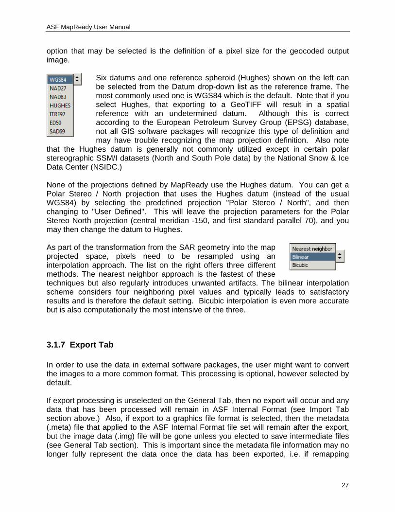
Six datums and one reference spheroid (Hughes) shown on the left can be selected from the Datum drop-down list as the reference frame. The most commonly used one is WGS84 which is the default. Note that if you select Hughes, that exporting to a GeoTIFF will result in a spatial reference with an undetermined datum. Although this is correct according to the European Petroleum Survey Group (EPSG) database, not all GIS software packages will recognize this type of definition and may have trouble recognizing the map projection definition. Also note
that the Hughes datum is generally not commonly utilized except in certain polar stereographic SSM/I datasets (North and South Pole data) by the National Snow & Ice Data Center (NSIDC.) None of the projections defined by MapReady use the Hughes datum. You can get a Polar Stereo / North projection that uses the Hughes datum (instead of the usual WGS84) by selecting the predefined projection "Polar Stereo / North", and then changing to "User Defined". This will leave the projection parameters for the Polar Stereo North projection (central meridian -150, and first standard parallel 70), and you may then change the datum to Hughes. As part of the transformation from the SAR geometry into the map projected space, pixels need to be resampled using an interpolation approach. The list on the right offers three different methods. The nearest neighbor approach is the fastest of these techniques but also regularly introduces unwanted artifacts. The bilinear interpolation scheme considers four neighboring pixel values and typically leads to satisfactory results and is therefore the default setting. Bicubic interpolation is even more accurate but is also computationally the most intensive of the three.
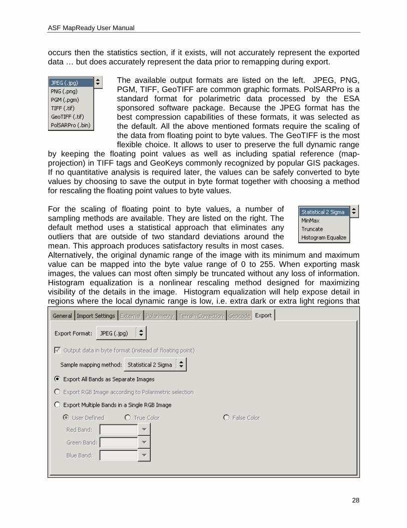
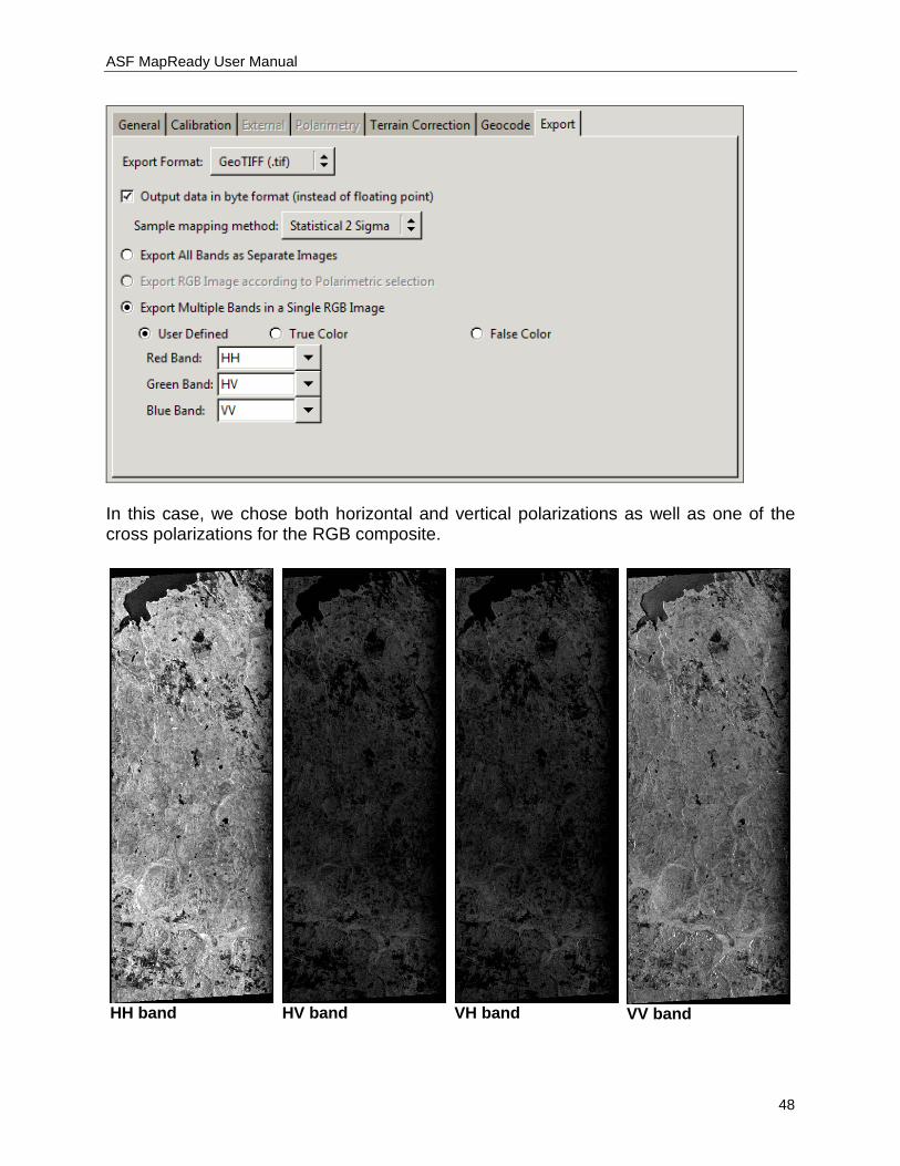
3.1.7 Export Tab In order to use the data in external software packages, the user might want to convert the images to a more common format. This processing is optional, however selected by default. If export processing is unselected on the General Tab, then no export will occur and any data that has been processed will remain in ASF Internal Format (see Import Tab section above.) Also, if export to a graphics file format is selected, then the metadata (.meta) file that applied to the ASF Internal Format file set will remain after the export, but the image data (.img) file will be gone unless you elected to save intermediate files (see General Tab section). This is important since the metadata file information may no longer fully represent the data once the data has been exported, i.e. if remapping
ASF MapReady User Manual
28
occurs then the statistics section, if it exists, will not accurately represent the exported data … but does accurately represent the data prior to remapping during export.
The available output formats are listed on the left. JPEG, PNG, PGM, TIFF, GeoTIFF are common graphic formats. PolSARPro is a standard format for polarimetric data processed by the ESA sponsored software package. Because the JPEG format has the best compression capabilities of these formats, it was selected as the default. All the above mentioned formats require the scaling of the data from floating point to byte values. The GeoTIFF is the most flexible choice. It allows to user to preserve the full dynamic range
by keeping the floating point values as well as including spatial reference (map-projection) in TIFF tags and GeoKeys commonly recognized by popular GIS packages. If no quantitative analysis is required later, the values can be safely converted to byte values by choosing to save the output in byte format together with choosing a method for rescaling the floating point values to byte values. For the scaling of floating point to byte values, a number of sampling methods are available. They are listed on the right. The default method uses a statistical approach that eliminates any outliers that are outside of two standard deviations around the mean. This approach produces satisfactory results in most cases. Alternatively, the original dynamic range of the image with its minimum and maximum value can be mapped into the byte value range of 0 to 255. When exporting mask images, the values can most often simply be truncated without any loss of information. Histogram equalization is a nonlinear rescaling method designed for maximizing visibility of the details in the image. Histogram equalization will help expose detail in regions where the local dynamic range is low, i.e. extra dark or extra light regions that
ASF MapReady User Manual
29
tend to hide fine detail will have the local contrast expanded over a broader range of values which highlights detail previously difficult to see. For images containing multiple bands, the user may select exporting each band or channel to a separate file, i.e. each color (optical) or polarization (SAR) channel, or to a color file (if supported by the selected graphics file type.) In addition to being able to manually select which color band individual channels are mapped to, for polarimetric data several predefined settings are available, as selected on the "Polarimetry" tab. If you have selected a polarimetric decomposition, you will not be able to select RGB channel assignments; the only option available is "Export Image According to Polarimetric Selection". The exception to this is the Entropy/Anisotropy/Alpha decomposition (Cloude-Pottier without classification), when you may assign each of the classification parameters to an RGB channel, or export each as a separate grayscale image. For optical images, you may also select True Color or False Color output types. If True Color is selected, band 03 will be assigned to the red band, 02 to the green band, and 01 to the blue band. If False Color is selected, then band 04 (near-IR) will be assigned to the red band, 03 to the green band, and 02 to the blue band. Additionally, whenever True Color or False Color is selected, each color band is individually contrast-expanded using a 2-sigma contrast expansion derived from each band’s individual statistics.
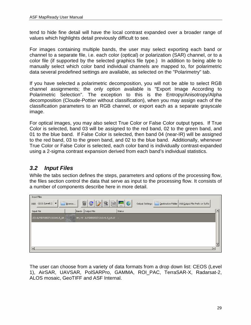
3.2 Input Files While the tabs section defines the steps, parameters and options of the processing flow, the files section control the data that serve as input to the processing flow. It consists of a number of components describe here in more detail.
The user can choose from a variety of data formats from a drop down list: CEOS (Level 1), AirSAR, UAVSAR, PolSARPro, GAMMA, ROI_PAC, TerraSAR-X, Radarsat-2, ALOS mosaic, GeoTIFF and ASF Internal.
ASF MapReady User Manual
30
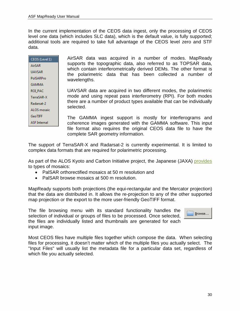
In the current implementation of the CEOS data ingest, only the processing of CEOS level one data (which includes SLC data), which is the default value, is fully supported; additional tools are required to take full advantage of the CEOS level zero and STF data.
AirSAR data was acquired in a number of modes. MapReady supports the topographic data, also referred to as TOPSAR data, which contain interferometrically derived DEMs. The other format is the polarimetric data that has been collected a number of wavelengths. UAVSAR data are acquired in two different modes, the polarimetric mode and using repeat pass interferometry (RPI). For both modes there are a number of product types available that can be individually selected. The GAMMA ingest support is mostly for interferograms and coherence images generated with the GAMMA software. This input file format also requires the original CEOS data file to have the complete SAR geometry information.
The support of TerraSAR-X and Radarsat-2 is currently experimental. It is limited to complex data formats that are required for polarimetric processing. As part of the ALOS Kyoto and Carbon Initiative project, the Japanese (JAXA) provides to types of mosaics:
• PalSAR orthorectified mosaics at 50 m resolution and • PalSAR browse mosaics at 500 m resolution.
MapReady supports both projections (the equi-rectangular and the Mercator projection) that the data are distributed in. It allows the re-projection to any of the other supported map projection or the export to the more user-friendly GeoTIFF format. The file browsing menu with its standard functionality handles the selection of individual or groups of files to be processed. Once selected, the files are individually listed and thumbnails are generated for each input image. Most CEOS files have multiple files together which compose the data. When selecting files for processing, it doesn’t matter which of the multiple files you actually select. The "Input Files" will usually list the metadata file for a particular data set, regardless of which file you actually selected.
ASF MapReady User Manual
31
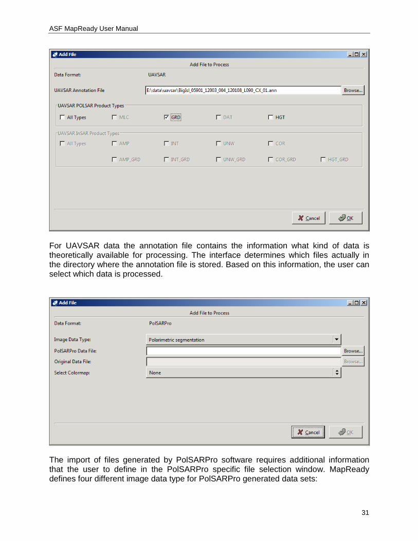
For UAVSAR data the annotation file contains the information what kind of data is theoretically available for processing. The interface determines which files actually in the directory where the annotation file is stored. Based on this information, the user can select which data is processed.
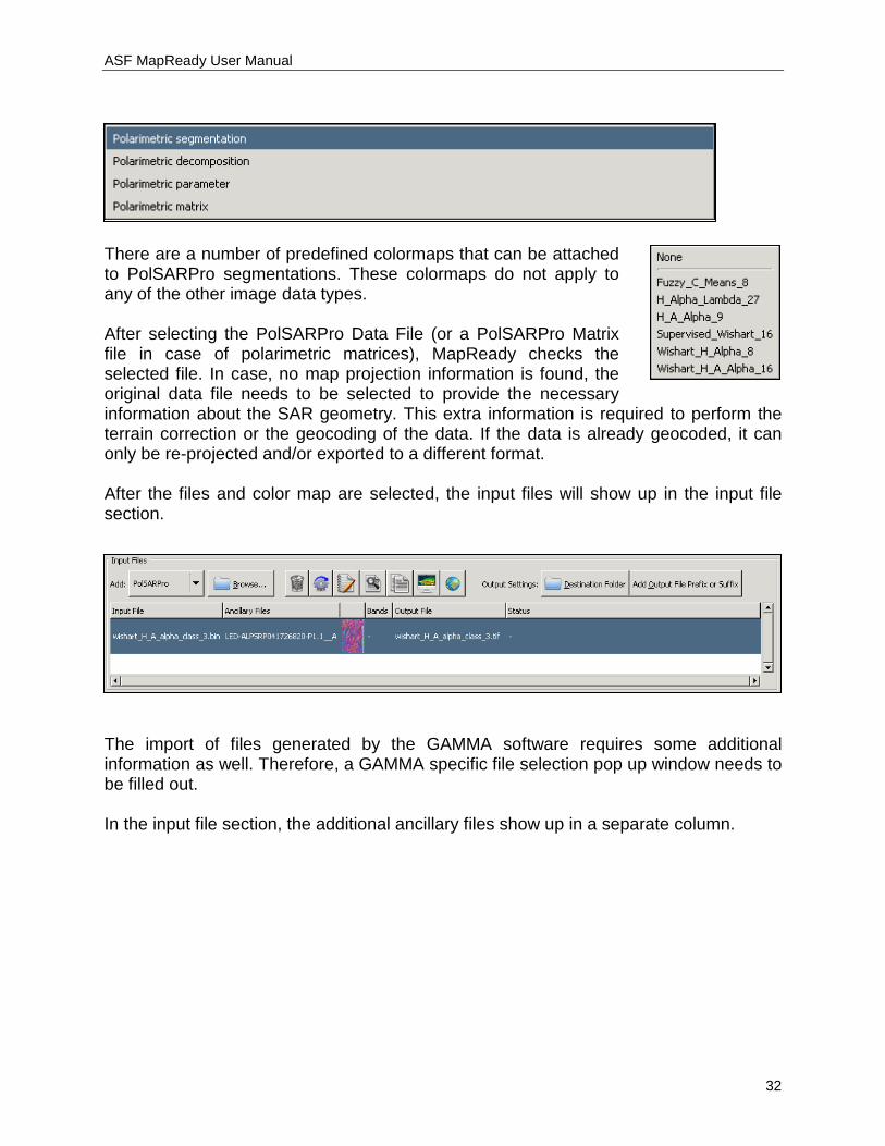
The import of files generated by PolSARPro software requires additional information that the user to define in the PolSARPro specific file selection window. MapReady defines four different image data type for PolSARPro generated data sets:
ASF MapReady User Manual
32
There are a number of predefined colormaps that can be attached to PolSARPro segmentations. These colormaps do not apply to any of the other image data types. After selecting the PolSARPro Data File (or a PolSARPro Matrix file in case of polarimetric matrices), MapReady checks the selected file. In case, no map projection information is found, the original data file needs to be selected to provide the necessary information about the SAR geometry. This extra information is required to perform the terrain correction or the geocoding of the data. If the data is already geocoded, it can only be re-projected and/or exported to a different format. After the files and color map are selected, the input files will show up in the input file section.
The import of files generated by the GAMMA software requires some additional information as well. Therefore, a GAMMA specific file selection pop up window needs to be filled out. In the input file section, the additional ancillary files show up in a separate column.

ASF MapReady User Manual
33
ROI_PAC is another SAR interferometric software whose data can be ingested in MapReady. As the ROI_PAC scripts follow predefined naming conventions, the ingest function only requires a metadata file (.rsc).
Immediately to the right of the "Browse" button is a toolbar containing buttons to help to get the data sets organized for the processing.
The "Remove" button deletes a file from the processing list. This becomes necessary, for example, when the input thumbnails, even though they are small, reveal that the selected image does not contain a certain feature or the area of
interest. All selected files are removed.
The "Process" button starts the processing of the selected data set rather than processing the entire list of files (see "Execute" button for details). This feature is particularly useful when a few data sets out of a long list did not successfully
process with the current sets of options and parameters. After selecting the appropriate values the data sets can be individually re-run using this feature.
The "Rename" button lets the user individually rename the output images of a run. This feature is mostly used when the same input data set is run with different options and parameters without overwriting any of the previous results. For
renaming a large number of files see the details on naming schemes.

ASF MapReady User Manual
34
The "View log" button allows the user to display the log file once a data set has been processed. The log file contains the feedback from the individual functions called as part of the processing flow. The log file is the single most useful piece
of information for troubleshooting problems as it contains the error messages that the tool issues in case the processing needs to be aborted.
The "Display CEOS metadata" button launches the ASF metadata viewer. The viewer reads the CEOS leader file, a partially binary and partially ASCII file that contains the metadata associated with the binary data (see Viewing the Leader
Data below.)
The "View Input" button launches the ASF viewer (asf_view) to view the selected input file.
The "Display in Google Earth" button launches Google Earth™, zooms to the image location on
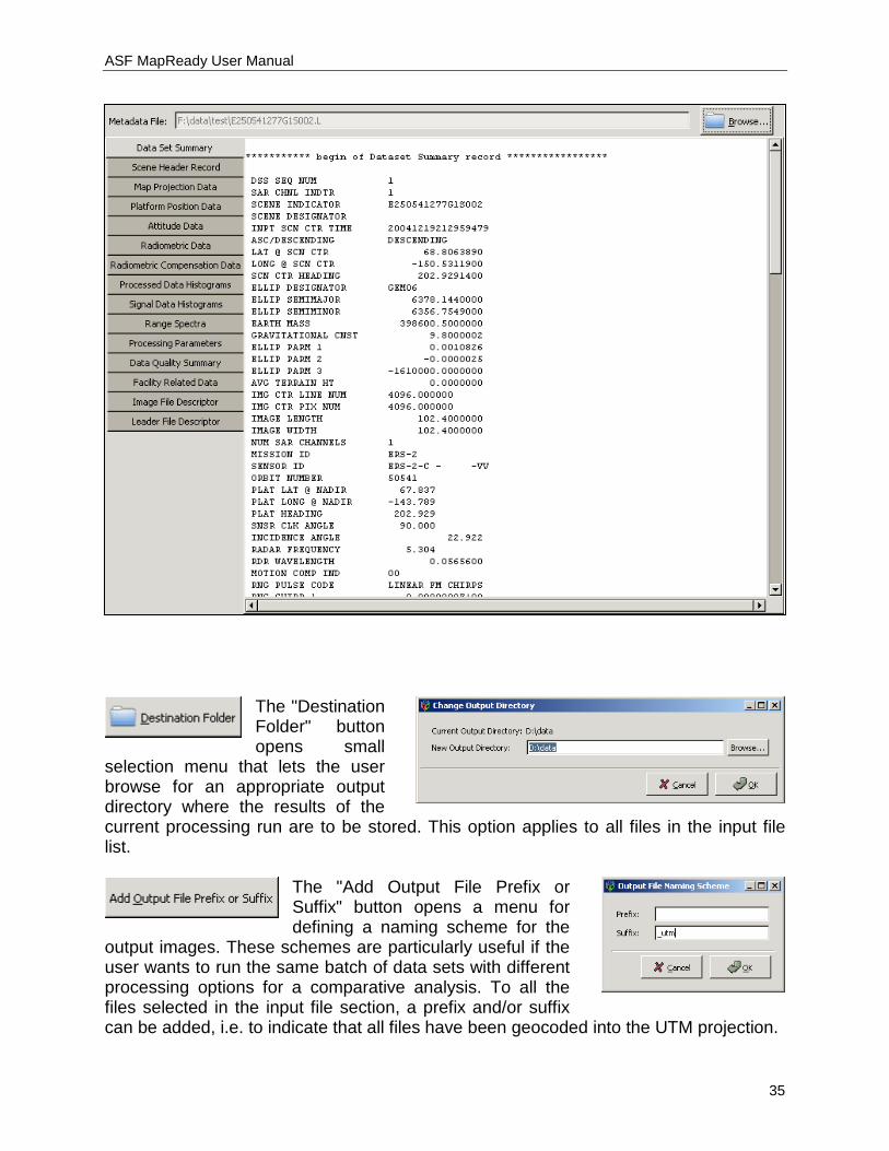
the Google Earth globe, and displays a blue box which illustrates the image boundaries. The functionality of the toolbar menu buttons is also available as a right mouse click context menu (as shown on the left) if you right-click on a selected input file. Viewing the Leader Data As mentioned above, clicking the "Display CEOS metadata" toolbar button (or, selecting that option from the right-click context menu) will launch the metadata viewer for viewing the CEOS leader file contents. The leader file is defined by a number of data records. The data set summary record provides general information about the image such as orbit and frame number, acquisition date, image size and sensor characteristics. The platform position data record contains orbital information in form of state vectors that describe the position of the satellite at a given time.
ASF MapReady User Manual
35
The "Destination Folder" button opens small
selection menu that lets the user browse for an appropriate output directory where the results of the current processing run are to be stored. This option applies to all files in the input file list.
The "Add Output File Prefix or Suffix" button opens a menu for defining a naming scheme for the
output images. These schemes are particularly useful if the user wants to run the same batch of data sets with different processing options for a comparative analysis. To all the files selected in the input file section, a prefix and/or suffix can be added, i.e. to indicate that all files have been geocoded into the UTM projection.
ASF MapReady User Manual
36
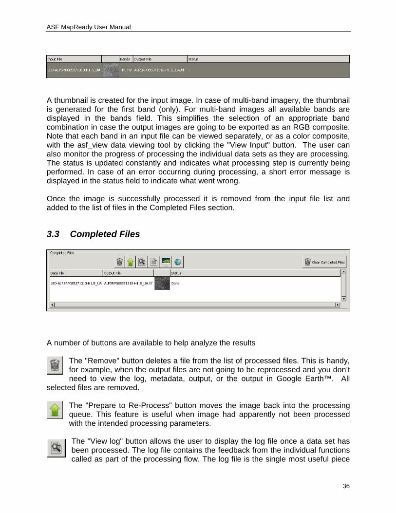
A thumbnail is created for the input image. In case of multi-band imagery, the thumbnail is generated for the first band (only). For multi-band images all available bands are displayed in the bands field. This simplifies the selection of an appropriate band combination in case the output images are going to be exported as an RGB composite. Note that each band in an input file can be viewed separately, or as a color composite, with the asf_view data viewing tool by clicking the "View Input" button. The user can also monitor the progress of processing the individual data sets as they are processing. The status is updated constantly and indicates what processing step is currently being performed. In case of an error occurring during processing, a short error message is displayed in the status field to indicate what went wrong. Once the image is successfully processed it is removed from the input file list and added to the list of files in the Completed Files section.
3.3 Completed Files
A number of buttons are available to help analyze the results
The "Remove" button deletes a file from the list of processed files. This is handy, for example, when the output files are not going to be reprocessed and you don’t need to view the log, metadata, output, or the output in Google Earth™. All
selected files are removed.
The "Prepare to Re-Process" button moves the image back into the processing queue. This feature is useful when image had apparently not been processed with the intended processing parameters.
The "View log" button allows the user to display the log file once a data set has been processed. The log file contains the feedback from the individual functions called as part of the processing flow. The log file is the single most useful piece
ASF MapReady User Manual
37
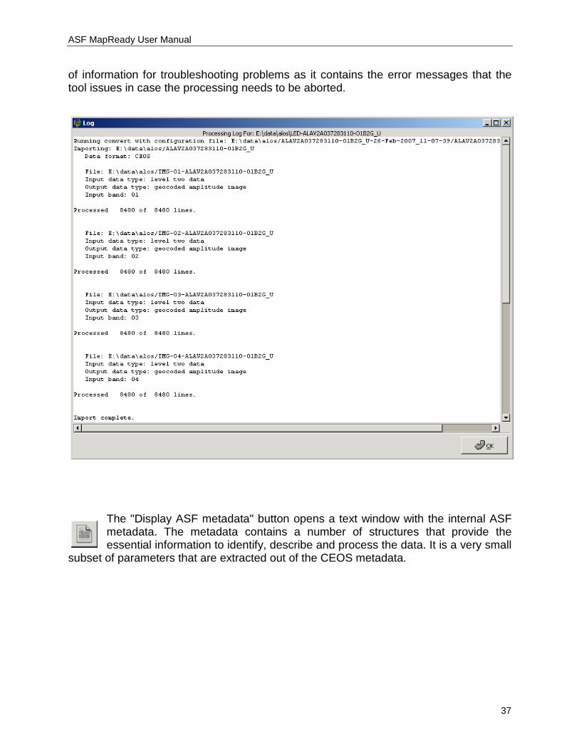
of information for troubleshooting problems as it contains the error messages that the tool issues in case the processing needs to be aborted.
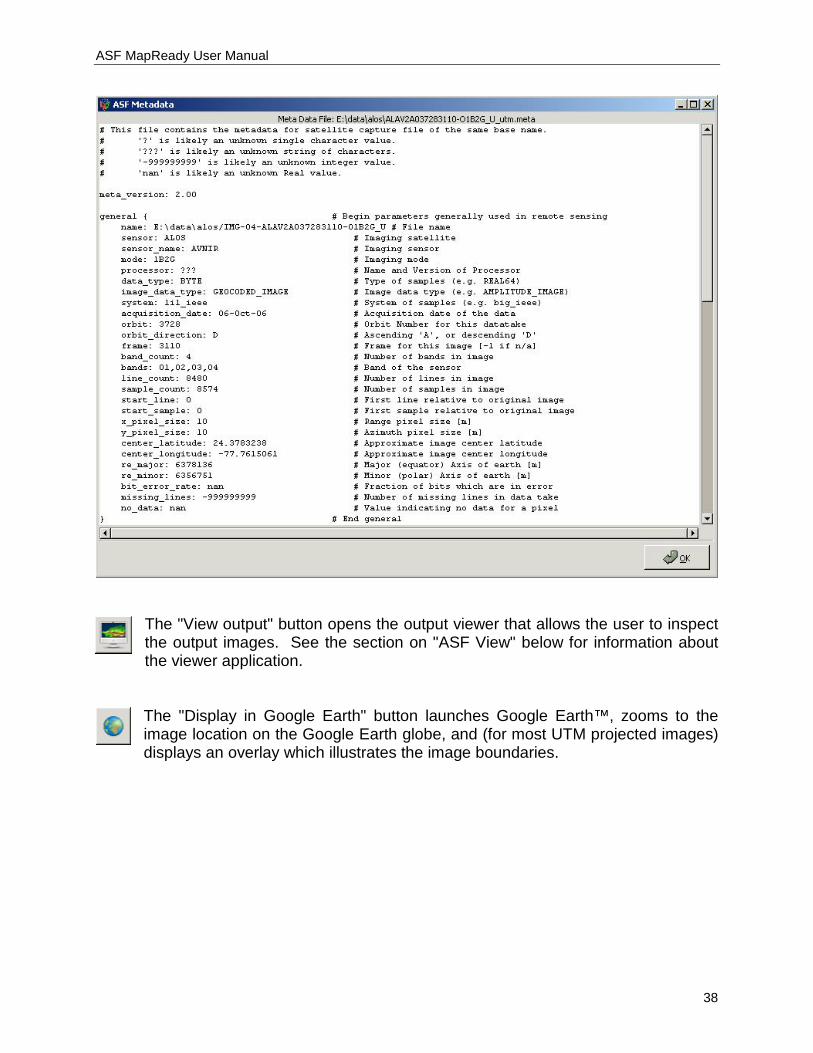
The "Display ASF metadata" button opens a text window with the internal ASF metadata. The metadata contains a number of structures that provide the essential information to identify, describe and process the data. It is a very small
subset of parameters that are extracted out of the CEOS metadata.
ASF MapReady User Manual
38
The "View output" button opens the output viewer that allows the user to inspect the output images. See the section on "ASF View" below for information about the viewer application.
The "Display in Google Earth" button launches Google Earth™, zooms to the image location on the Google Earth globe, and (for most UTM projected images) displays an overlay which illustrates the image boundaries.
ASF MapReady User Manual
39
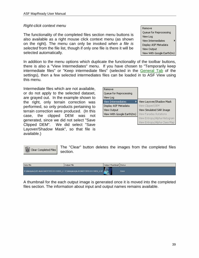
Right-click context menu The functionality of the completed files section menu buttons is also available as a right mouse click context menu (as shown on the right). The menu can only be invoked when a file is selected from the file list, though if only one file is there it will be selected automatically. In addition to the menu options which duplicate the functionality of the toolbar buttons, there is also a "View Intermediates" menu. If you have chosen to "Temporarily keep intermediate files" or "Keep intermediate files" (selected in the General Tab of the settings), then a few selected intermediates files can be loaded in to ASF View using this menu. Intermediate files which are not available, or do not apply to the selected dataset, are grayed out. In the example shown to the right, only terrain correction was performed, so only products pertaining to terrain correction were produced. (In this case, the clipped DEM was not generated, since we did not select "Save Clipped DEM". We did select "Save Layover/Shadow Mask", so that file is available.)
The "Clear" button deletes the images from the completed files section.
A thumbnail for the each output image is generated once it is moved into the completed files section. The information about input and output names remains available.
ASF MapReady User Manual
40
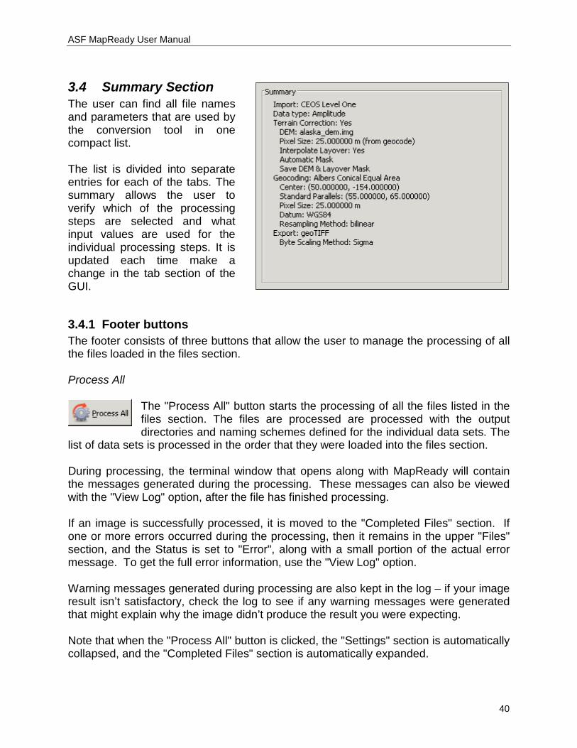
3.4 Summary Section The user can find all file names and parameters that are used by the conversion tool in one compact list. The list is divided into separate entries for each of the tabs. The summary allows the user to verify which of the processing steps are selected and what input values are used for the individual processing steps. It is updated each time make a change in the tab section of the GUI.
3.4.1 Footer buttons The footer consists of three buttons that allow the user to manage the processing of all the files loaded in the files section. Process All
The "Process All" button starts the processing of all the files listed in the files section. The files are processed are processed with the output directories and naming schemes defined for the individual data sets. The
list of data sets is processed in the order that they were loaded into the files section. During processing, the terminal window that opens along with MapReady will contain the messages generated during the processing. These messages can also be viewed with the "View Log" option, after the file has finished processing. If an image is successfully processed, it is moved to the "Completed Files" section. If one or more errors occurred during the processing, then it remains in the upper "Files" section, and the Status is set to "Error", along with a small portion of the actual error message. To get the full error information, use the "View Log" option. Warning messages generated during processing are also kept in the log – if your image result isn’t satisfactory, check the log to see if any warning messages were generated that might explain why the image didn’t produce the result you were expecting. Note that when the "Process All" button is clicked, the "Settings" section is automatically collapsed, and the "Completed Files" section is automatically expanded.
ASF MapReady User Manual
41
Stop Processing
The "Stop Processing" button interrupts the processing of the list of data sets. The image that is currently being processed will stop with a "Processing Stopped By User" error, though any data files that have
already completed are left in the "Completed Files" section. It may take a moment for the processing to stop. Help
The "Help" button opens the PDF file of this manual.
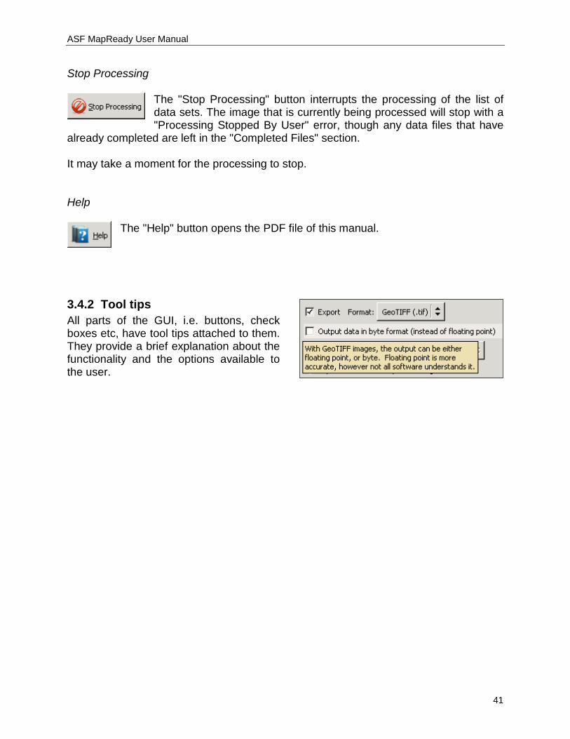
3.4.2 Tool tips All parts of the GUI, i.e. buttons, check boxes etc, have tool tips attached to them. They provide a brief explanation about the functionality and the options available to the user.

ASF MapReady User Manual
42
3.5 Examples In this section some of the most common uses of the MapReady tool are demonstrated.
3.5.1 Converting optical ALOS AVNIR data into GeoTIFF format
Band 1 Band 2
Band 3 Band 4 The AVNIR instrument on the ALOS satellite is a four-band (visible-and near-infrared) radiometer with a resolution of 10 m, designed for observing land and coastal zones.
ASF MapReady User Manual
43
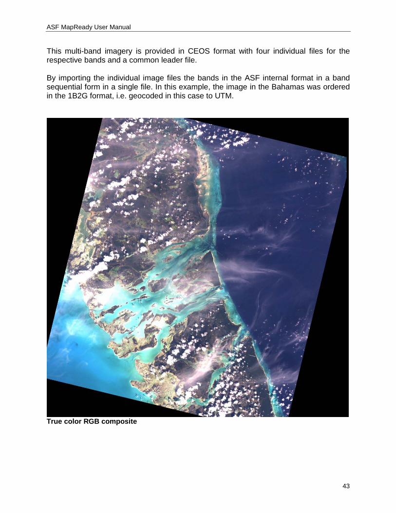
This multi-band imagery is provided in CEOS format with four individual files for the respective bands and a common leader file. By importing the individual image files the bands in the ASF internal format in a band sequential form in a single file. In this example, the image in the Bahamas was ordered in the 1B2G format, i.e. geocoded in this case to UTM.
True color RGB composite
ASF MapReady User Manual
44
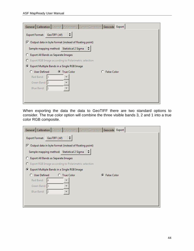
When exporting the data the data to GeoTIFF there are two standard options to consider. The true color option will combine the three visible bands 3, 2 and 1 into a true color RGB composite.
ASF MapReady User Manual
45
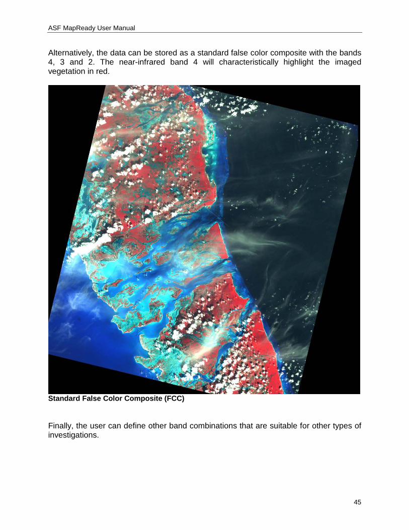
Alternatively, the data can be stored as a standard false color composite with the bands 4, 3 and 2. The near-infrared band 4 will characteristically highlight the imaged vegetation in red.
Standard False Color Composite (FCC) Finally, the user can define other band combinations that are suitable for other types of investigations.
ASF MapReady User Manual
46
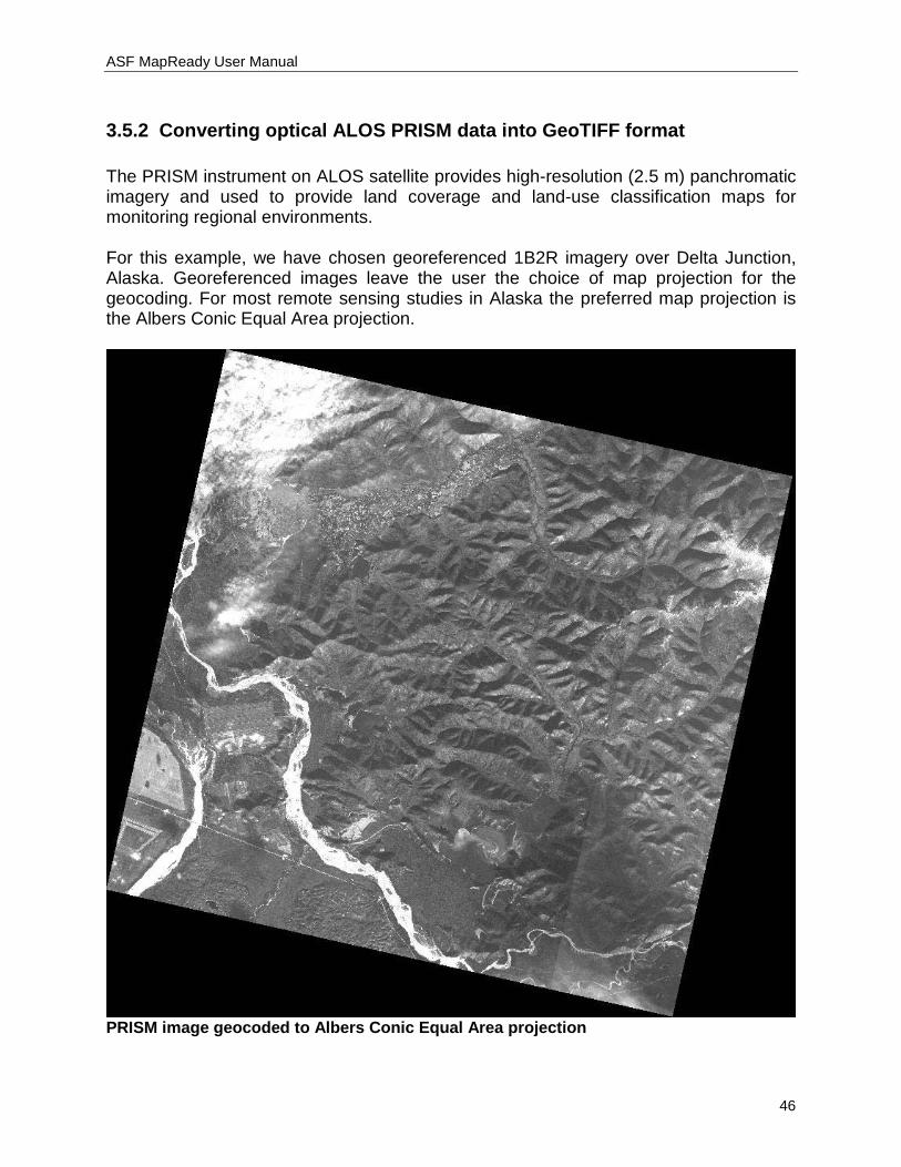
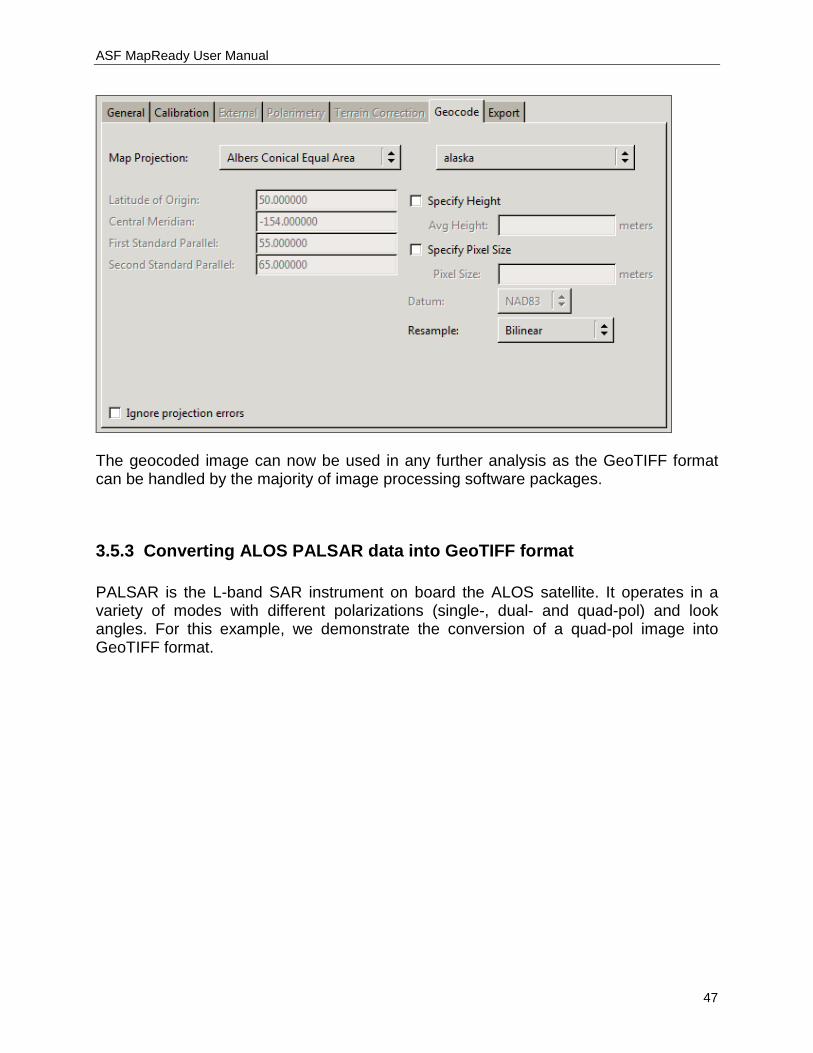
3.5.2 Converting optical ALOS PRISM data into GeoTIFF format The PRISM instrument on ALOS satellite provides high-resolution (2.5 m) panchromatic imagery and used to provide land coverage and land-use classification maps for monitoring regional environments. For this example, we have chosen georeferenced 1B2R imagery over Delta Junction, Alaska. Georeferenced images leave the user the choice of map projection for the geocoding. For most remote sensing studies in Alaska the preferred map projection is the Albers Conic Equal Area projection.
PRISM image geocoded to Albers Conic Equal Area projection
ASF MapReady User Manual
47
The geocoded image can now be used in any further analysis as the GeoTIFF format can be handled by the majority of image processing software packages.
3.5.3 Converting ALOS PALSAR data into GeoTIFF format PALSAR is the L-band SAR instrument on board the ALOS satellite. It operates in a variety of modes with different polarizations (single-, dual- and quad-pol) and look angles. For this example, we demonstrate the conversion of a quad-pol image into GeoTIFF format.
ASF MapReady User Manual
48
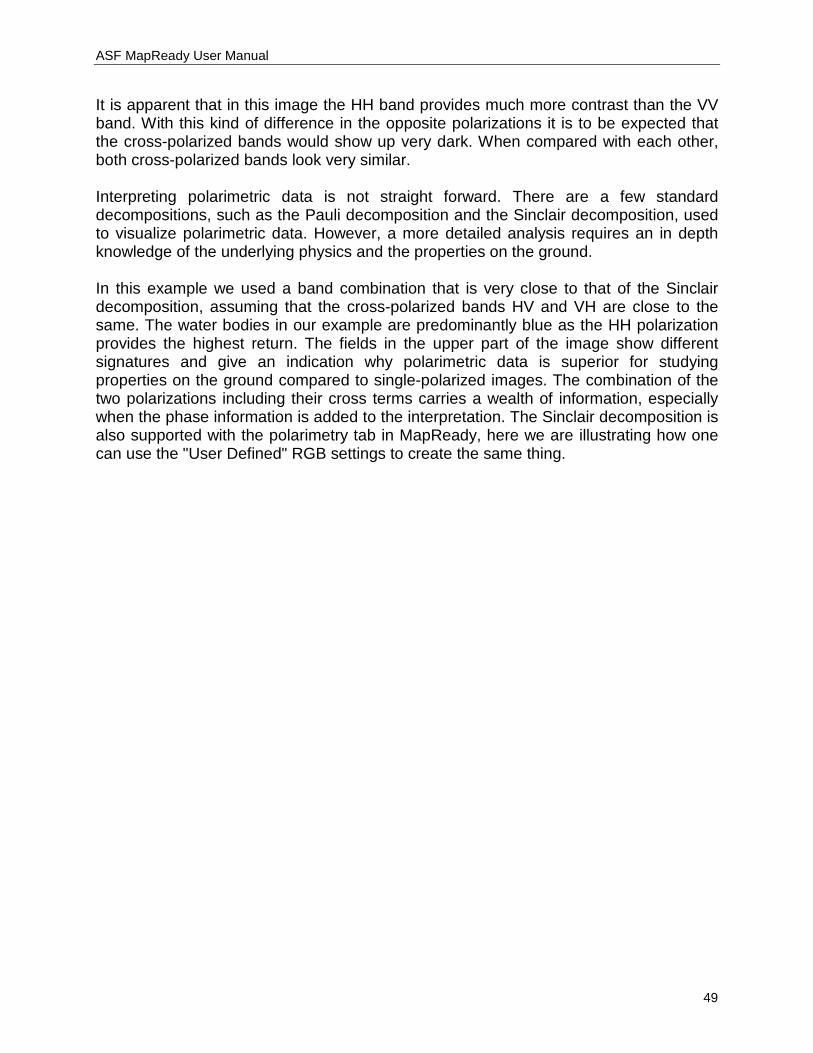
In this case, we chose both horizontal and vertical polarizations as well as one of the cross polarizations for the RGB composite.
HH band HV band VH band VV band
ASF MapReady User Manual
49
It is apparent that in this image the HH band provides much more contrast than the VV band. With this kind of difference in the opposite polarizations it is to be expected that the cross-polarized bands would show up very dark. When compared with each other, both cross-polarized bands look very similar. Interpreting polarimetric data is not straight forward. There are a few standard decompositions, such as the Pauli decomposition and the Sinclair decomposition, used to visualize polarimetric data. However, a more detailed analysis requires an in depth knowledge of the underlying physics and the properties on the ground. In this example we used a band combination that is very close to that of the Sinclair decomposition, assuming that the cross-polarized bands HV and VH are close to the same. The water bodies in our example are predominantly blue as the HH polarization provides the highest return. The fields in the upper part of the image show different signatures and give an indication why polarimetric data is superior for studying properties on the ground compared to single-polarized images. The combination of the two polarizations including their cross terms carries a wealth of information, especially when the phase information is added to the interpretation. The Sinclair decomposition is also supported with the polarimetry tab in MapReady, here we are illustrating how one can use the "User Defined" RGB settings to create the same thing.

ASF MapReady User Manual
50
PALSAR RGB composite (HH, HV, VV)
ASF MapReady User Manual
51
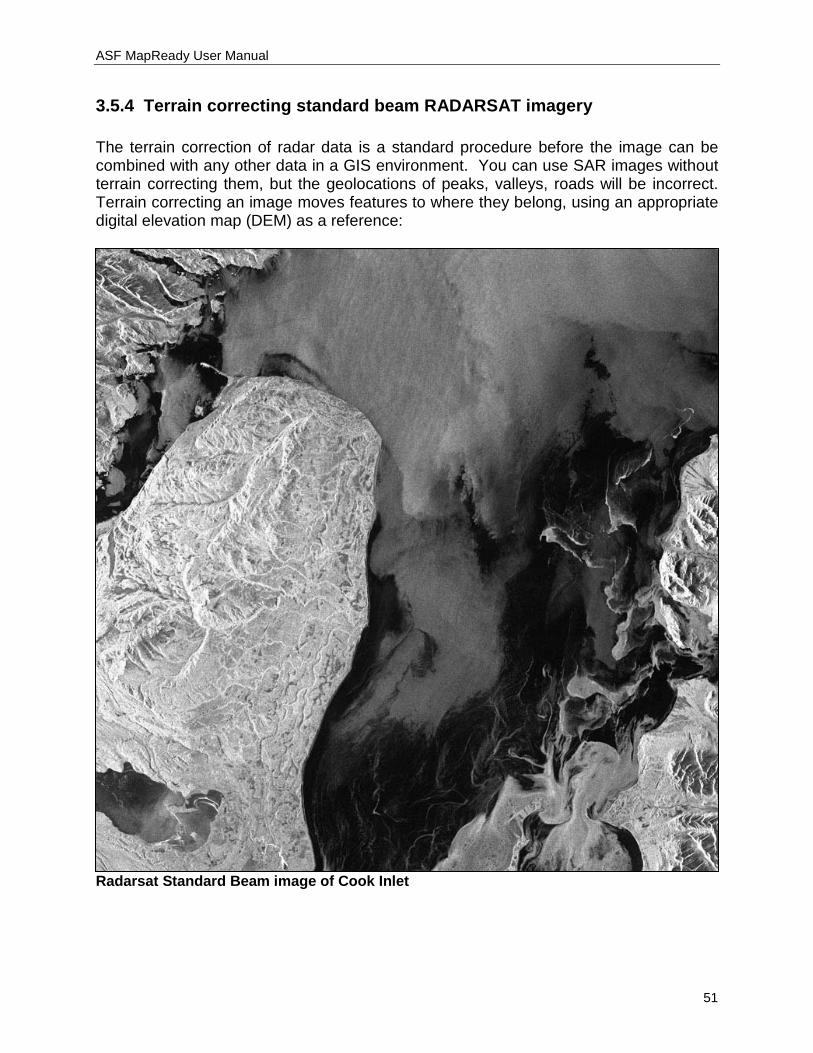
3.5.4 Terrain correcting standard beam RADARSAT imagery The terrain correction of radar data is a standard procedure before the image can be combined with any other data in a GIS environment. You can use SAR images without terrain correcting them, but the geolocations of peaks, valleys, roads will be incorrect. Terrain correcting an image moves features to where they belong, using an appropriate digital elevation map (DEM) as a reference:
Radarsat Standard Beam image of Cook Inlet
ASF MapReady User Manual
52
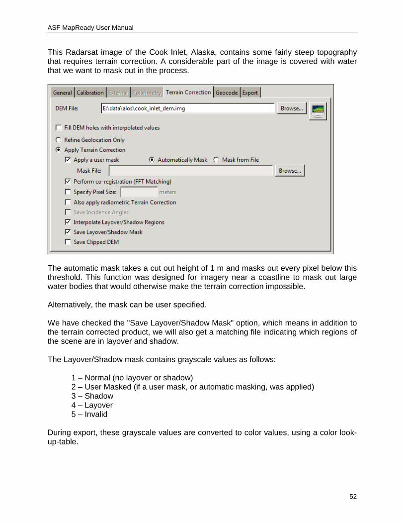
This Radarsat image of the Cook Inlet, Alaska, contains some fairly steep topography that requires terrain correction. A considerable part of the image is covered with water that we want to mask out in the process.
The automatic mask takes a cut out height of 1 m and masks out every pixel below this threshold. This function was designed for imagery near a coastline to mask out large water bodies that would otherwise make the terrain correction impossible. Alternatively, the mask can be user specified. We have checked the "Save Layover/Shadow Mask" option, which means in addition to the terrain corrected product, we will also get a matching file indicating which regions of the scene are in layover and shadow. The Layover/Shadow mask contains grayscale values as follows: 1 – Normal (no layover or shadow) 2 – User Masked (if a user mask, or automatic masking, was applied) 3 – Shadow 4 – Layover 5 – Invalid During export, these grayscale values are converted to color values, using a color look-up-table.
ASF MapReady User Manual
53
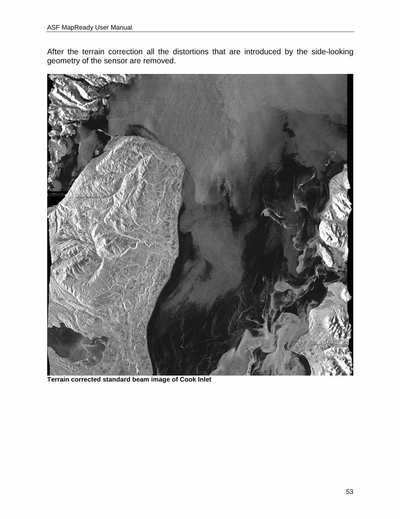
After the terrain correction all the distortions that are introduced by the side-looking geometry of the sensor are removed.
Terrain corrected standard beam image of Cook Inlet
ASF MapReady User Manual
54
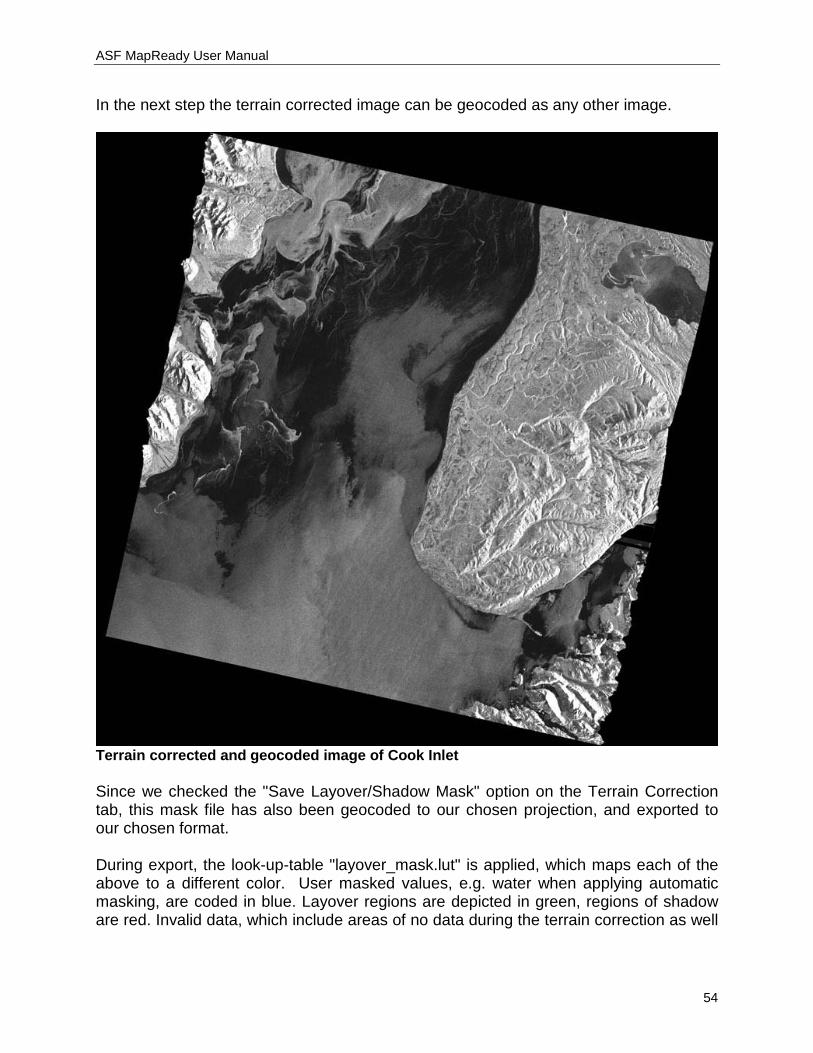
In the next step the terrain corrected image can be geocoded as any other image.
Terrain corrected and geocoded image of Cook Inlet Since we checked the "Save Layover/Shadow Mask" option on the Terrain Correction tab, this mask file has also been geocoded to our chosen projection, and exported to our chosen format. During export, the look-up-table "layover_mask.lut" is applied, which maps each of the above to a different color. User masked values, e.g. water when applying automatic masking, are coded in blue. Layover regions are depicted in green, regions of shadow are red. Invalid data, which include areas of no data during the terrain correction as well
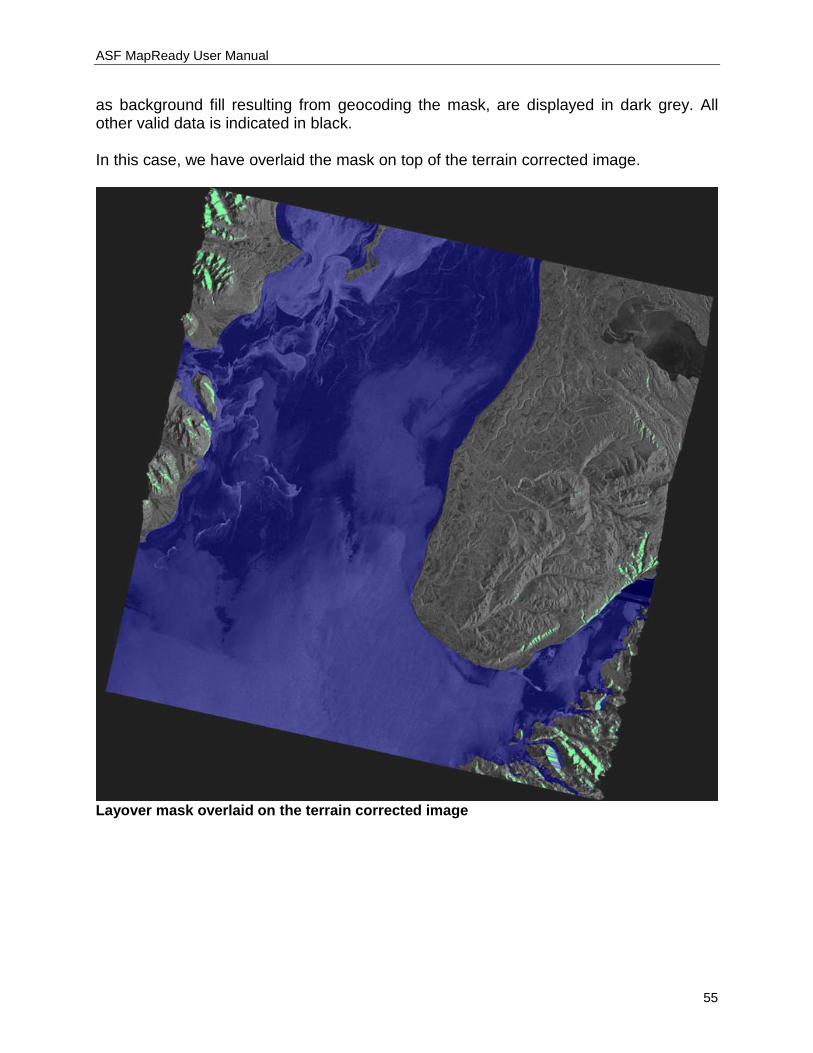
ASF MapReady User Manual
55
as background fill resulting from geocoding the mask, are displayed in dark grey. All other valid data is indicated in black. In this case, we have overlaid the mask on top of the terrain corrected image.
Layover mask overlaid on the terrain corrected image
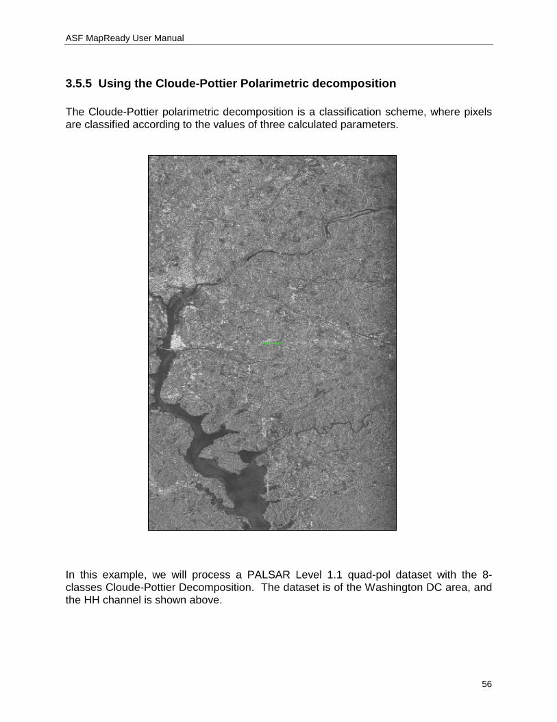
ASF MapReady User Manual
56
3.5.5 Using the Cloude-Pottier Polarimetric decomposition
The Cloude-Pottier polarimetric decomposition is a classification scheme, where pixels are classified according to the values of three calculated parameters.
In this example, we will process a PALSAR Level 1.1 quad-pol dataset with the 8-classes Cloude-Pottier Decomposition. The dataset is of the Washington DC area, and the HH channel is shown above.

ASF MapReady User Manual
57
In this example, we will not apply Terrain Correction or Geocoding, though both of these do work on SLC data, including SLC data to which you’ve applied a polarimetric decomposition. The results of the processing are shown below:
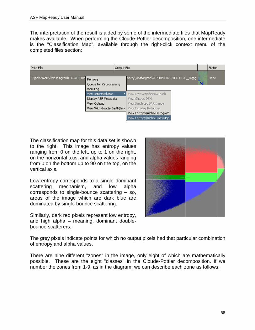
ASF MapReady User Manual
58
The interpretation of the result is aided by some of the intermediate files that MapReady makes available. When performing the Cloude-Pottier decomposition, one intermediate is the "Classification Map", available through the right-click context menu of the completed files section:
The classification map for this data set is shown to the right. This image has entropy values ranging from 0 on the left, up to 1 on the right, on the horizontal axis; and alpha values ranging from 0 on the bottom up to 90 on the top, on the vertical axis. Low entropy corresponds to a single dominant scattering mechanism, and low alpha corresponds to single-bounce scattering – so, areas of the image which are dark blue are dominated by single-bounce scattering. Similarly, dark red pixels represent low entropy, and high alpha – meaning, dominant double-bounce scatterers. The grey pixels indicate points for which no output pixels had that particular combination of entropy and alpha values. There are nine different "zones" in the image, only eight of which are mathematically possible. These are the eight "classes" in the Cloude-Pottier decomposition. If we number the zones from 1-9, as in the diagram, we can describe each zone as follows:
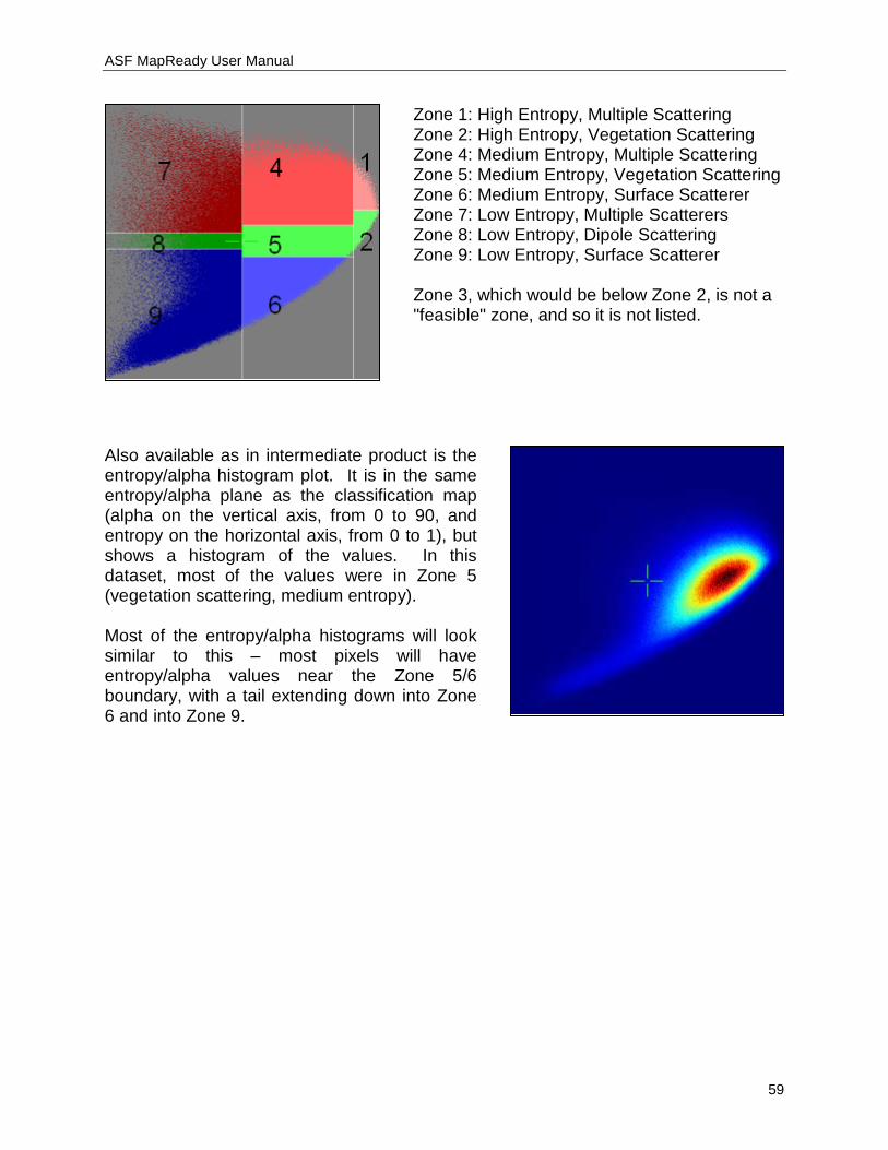
ASF MapReady User Manual
59
Zone 1: High Entropy, Multiple Scattering Zone 2: High Entropy, Vegetation Scattering Zone 4: Medium Entropy, Multiple Scattering Zone 5: Medium Entropy, Vegetation Scattering Zone 6: Medium Entropy, Surface Scatterer Zone 7: Low Entropy, Multiple Scatterers Zone 8: Low Entropy, Dipole Scattering Zone 9: Low Entropy, Surface Scatterer Zone 3, which would be below Zone 2, is not a "feasible" zone, and so it is not listed.
Also available as in intermediate product is the entropy/alpha histogram plot. It is in the same entropy/alpha plane as the classification map (alpha on the vertical axis, from 0 to 90, and entropy on the horizontal axis, from 0 to 1), but shows a histogram of the values. In this dataset, most of the values were in Zone 5 (vegetation scattering, medium entropy). Most of the entropy/alpha histograms will look similar to this – most pixels will have entropy/alpha values near the Zone 5/6 boundary, with a tail extending down into Zone 6 and into Zone 9.

ASF MapReady User Manual
60
3.5.6 Correcting Palsar for Faraday Rotation In L-band data, the ionosphere is assumed to have considerable effects on the SAR imagery. The anisotropy in the ionosphere due to charged particles in the presence of a persistent magnetic field causes the so called Faraday rotation. The Faraday rotation needs to be corrected for in order to avoid range shifts, internal image deformations, range and azimuth blurring in SAR images. It could cause azimuth streaking and phase error for SAR interferometry.
Palsar quad-pol amplitude (HH) Faraday rotation For more information on Faraday rotation, the user is referred to: Meyer, F.J. and Nicoll, J.B., 2008. Prediction, detection, and correction of Faraday
rotation in full-polarimetric L-band SAR data. IEEE Transactions on Geoscience and Remote Sensing, 46(10):3076-3086.
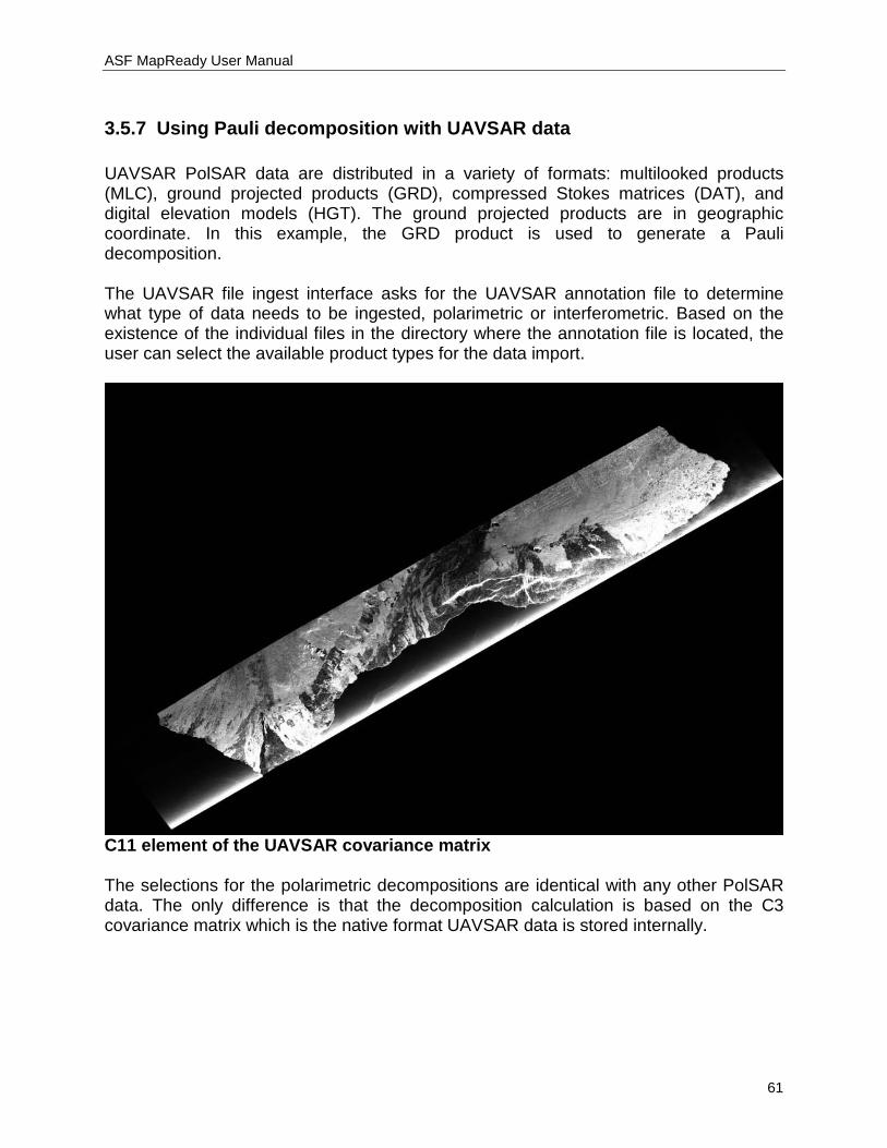
ASF MapReady User Manual
61
3.5.7 Using Pauli decomposition with UAVSAR data UAVSAR PolSAR data are distributed in a variety of formats: multilooked products (MLC), ground projected products (GRD), compressed Stokes matrices (DAT), and digital elevation models (HGT). The ground projected products are in geographic coordinate. In this example, the GRD product is used to generate a Pauli decomposition. The UAVSAR file ingest interface asks for the UAVSAR annotation file to determine what type of data needs to be ingested, polarimetric or interferometric. Based on the existence of the individual files in the directory where the annotation file is located, the user can select the available product types for the data import.
C11 element of the UAVSAR covariance matrix The selections for the polarimetric decompositions are identical with any other PolSAR data. The only difference is that the decomposition calculation is based on the C3 covariance matrix which is the native format UAVSAR data is stored internally.
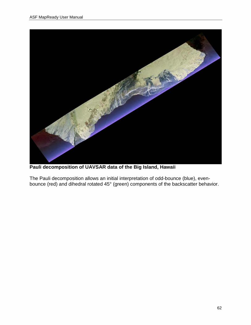
ASF MapReady User Manual
62
Pauli decomposition of UAVSAR data of the Big Island, Hawaii The Pauli decomposition allows an initial interpretation of odd-bounce (blue), even-bounce (red) and dihedral rotated 45° (green) components of the backscatter behavior.

ASF MapReady User Manual
63
4. The interface between MapReady and PolSARPro PolSARPro is the most comprehensive open-source software for processing PolSAR and PolInSAR data. It supports a large variety of space-borne and airborne data sources. However, PolSARPro does not have capabilities to terrain correct and/or geocode its results. For mitigating this shortcoming we have developed an interface that uses MapReady functionality for this task.
The two alternative processing flows for polarimetric data (Gens et al., 2013).
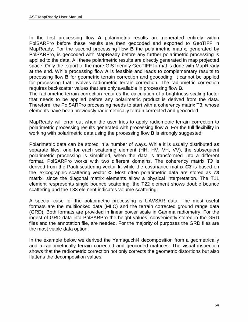
ASF MapReady User Manual
64
In the first processing flow A polarimetric results are generated entirely within PolSARPro before these results are then geocoded and exported to GeoTIFF in MapReady. For the second processing flow B the polarimetric matrix, generated by PolSARPro, is geocoded with MapReady before any further polarimetric processing is applied to the data. All these polarimetric results are directly generated in map projected space. Only the export to the more GIS friendly GeoTIFF format is done with MapReady at the end. While processing flow A is feasible and leads to complementary results to processing flow B for geometric terrain correction and geocoding, it cannot be applied for processing that involves radiometric terrain correction. The radiometric correction requires backscatter values that are only available in processing flow B. The radiometric terrain correction requires the calculation of a brightness scaling factor that needs to be applied before any polarimetric product is derived from the data. Therefore, the PolSARPro processing needs to start with a coherency matrix T3, whose elements have been previously radiometrically terrain corrected and geocoded. MapReady will error out when the user tries to apply radiometric terrain correction to polarimetric processing results generated with processing flow A. For the full flexibility in working with polarimetric data using the processing flow B is strongly suggested. Polarimetric data can be stored in a number of ways. While it is usually distributed as separate files, one for each scattering element (HH, HV, VH, VV), the subsequent polarimetric processing is simplified, when the data is transformed into a different format. PolSARPro works with two different domains. The coherency matrix T3 is derived from the Pauli scattering vector k, while the covariance matrix C3 is based on the lexicographic scattering vector Ω. Most often polarimetric data are stored as T3 matrix, since the diagonal matrix elements allow a physical interpretation. The T11 element respresents single bounce scattering, the T22 element shows double bounce scattering and the T33 element indicates volume scattering. A special case for the polarimetric processing is UAVSAR data. The most useful formats are the multilooked data (MLC) and the terrain corrected ground range data (GRD). Both formats are provided in linear power scale in Gamma radiometry. For the ingest of GRD data into PolSARPro the height values, conveniently stored in the GRD files and the annotation file, are needed. For the majority of purposes the GRD files are the most viable data option. In the example below we derived the Yamaguchi4 decomposition from a geometrically and a radiometrically terrain corrected and geocoded matrices. The visual inspection shows that the radiometric correction not only corrects the geometric distortions but also flattens the decomposition values.
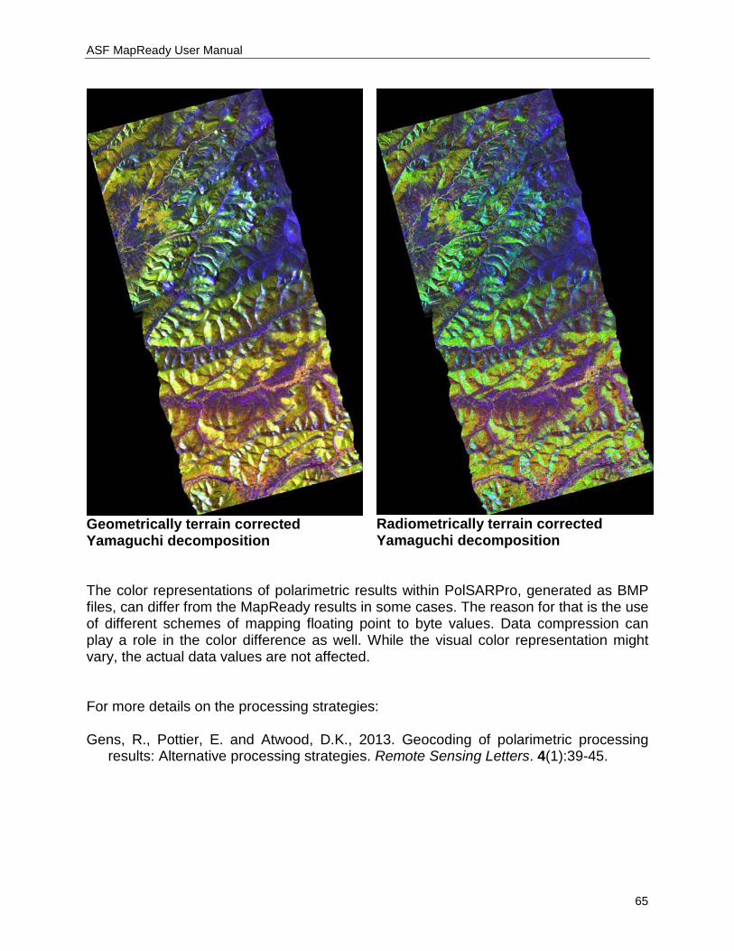
ASF MapReady User Manual
65
The color representations of polarimetric results within PolSARPro, generated as BMP files, can differ from the MapReady results in some cases. The reason for that is the use of different schemes of mapping floating point to byte values. Data compression can play a role in the color difference as well. While the visual color representation might vary, the actual data values are not affected. For more details on the processing strategies: Gens, R., Pottier, E. and Atwood, D.K., 2013. Geocoding of polarimetric processing
results: Alternative processing strategies. Remote Sensing Letters. 4(1):39-45.
Geometrically terrain corrected Yamaguchi decomposition
Radiometrically terrain corrected Yamaguchi decomposition
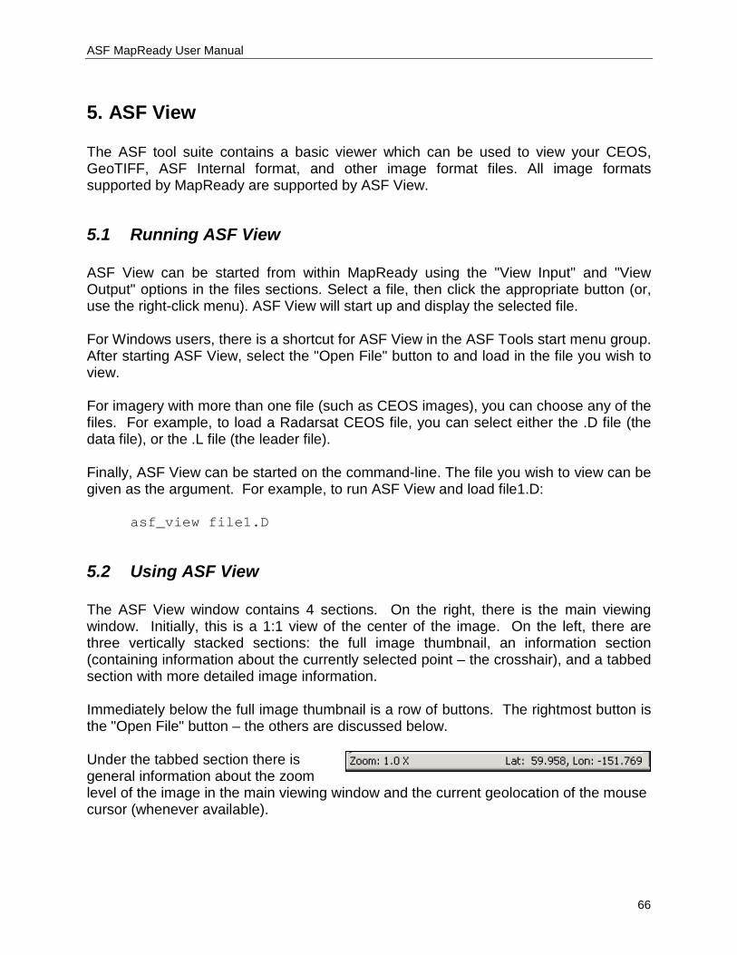
ASF MapReady User Manual
66
5. ASF View The ASF tool suite contains a basic viewer which can be used to view your CEOS, GeoTIFF, ASF Internal format, and other image format files. All image formats supported by MapReady are supported by ASF View.
5.1 Running ASF View ASF View can be started from within MapReady using the "View Input" and "View Output" options in the files sections. Select a file, then click the appropriate button (or, use the right-click menu). ASF View will start up and display the selected file. For Windows users, there is a shortcut for ASF View in the ASF Tools start menu group. After starting ASF View, select the "Open File" button to and load in the file you wish to view. For imagery with more than one file (such as CEOS images), you can choose any of the files. For example, to load a Radarsat CEOS file, you can select either the .D file (the data file), or the .L file (the leader file). Finally, ASF View can be started on the command-line. The file you wish to view can be given as the argument. For example, to run ASF View and load file1.D: asf_view file1.D
5.2 Using ASF View The ASF View window contains 4 sections. On the right, there is the main viewing window. Initially, this is a 1:1 view of the center of the image. On the left, there are three vertically stacked sections: the full image thumbnail, an information section (containing information about the currently selected point – the crosshair), and a tabbed section with more detailed image information. Immediately below the full image thumbnail is a row of buttons. The rightmost button is the "Open File" button – the others are discussed below. Under the tabbed section there is general information about the zoom level of the image in the main viewing window and the current geolocation of the mouse cursor (whenever available).
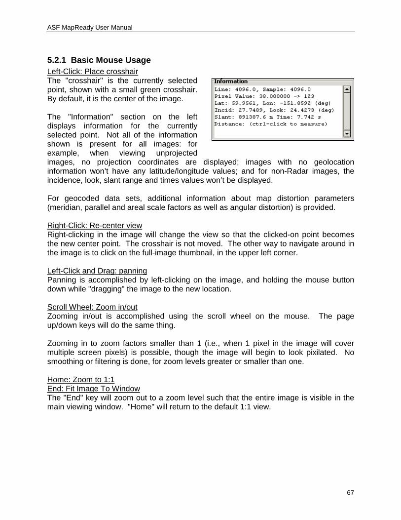
ASF MapReady User Manual
67
5.2.1 Basic Mouse Usage
The "crosshair" is the currently selected point, shown with a small green crosshair. By default, it is the center of the image.
Left-Click: Place crosshair
The "Information" section on the left displays information for the currently selected point. Not all of the information shown is present for all images: for example, when viewing unprojected images, no projection coordinates are displayed; images with no geolocation information won’t have any latitude/longitude values; and for non-Radar images, the incidence, look, slant range and times values won’t be displayed. For geocoded data sets, additional information about map distortion parameters (meridian, parallel and areal scale factors as well as angular distortion) is provided.
Right-clicking in the image will change the view so that the clicked-on point becomes the new center point. The crosshair is not moved. The other way to navigate around in the image is to click on the full-image thumbnail, in the upper left corner.
Right-Click: Re-center view
Panning is accomplished by left-clicking on the image, and holding the mouse button down while "dragging" the image to the new location.
Left-Click and Drag: panning
Zooming in/out is accomplished using the scroll wheel on the mouse. The page up/down keys will do the same thing.
Scroll Wheel: Zoom in/out
Zooming in to zoom factors smaller than 1 (i.e., when 1 pixel in the image will cover multiple screen pixels) is possible, though the image will begin to look pixilated. No smoothing or filtering is done, for zoom levels greater or smaller than one. Home: Zoom to 1:1
The "End" key will zoom out to a zoom level such that the entire image is visible in the main viewing window. "Home" will return to the default 1:1 view.
End: Fit Image To Window

ASF MapReady User Manual
68
5.2.2 Defining Polygons
Holding "ctrl" while left-clicking will place a red crosshair. This secondary crosshair can be used to measure distances. After placing the secondary crosshair, the distance between the two points is displayed in the information section.
Ctrl-Left-Click: Place secondary crosshair(s)
More than one secondary crosshair can be placed. This will define a polygon, and the total length and the enclosed area of the polygon is displayed in the information section. Backspace: Remove last ctrl-clicked point
Erroneous or badly placed ctrl-clicked points can be cleared using Backspace (clears the last point added) and Escape (clears the entire path).
Esc: Clear ctrl-clicked path
To fine-tune the positioning of selected points, use the arrow keys. By default, the most recently positioned point is moved. Using "ctrl" and/or "shift" with the arrow key will move the crosshair by a larger amount. (ctrl-arrow: 10 pixels, shift-arrow: 25 pixels, ctrl-shift-arrow: 250 pixels)
Arrow Keys: Move crosshair 1x
The "tab" key will change the point that is moved when the arrow keys are used. Tab: Toggle which crosshair is moved
To illustrate how defining polygons works, we will measure the circumference of the field in the image to the right. We start by left-clicking on the top left corner. If we miss the point, we can use the arrow keys to fine-tune the location. If necessary, we could zoom in to ensure that we’ve got the actual corner.
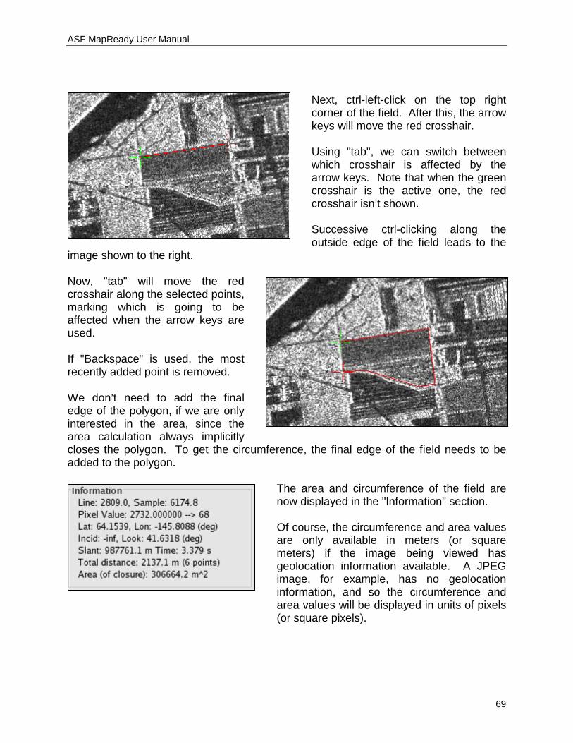
ASF MapReady User Manual
69
Next, ctrl-left-click on the top right corner of the field. After this, the arrow keys will move the red crosshair. Using "tab", we can switch between which crosshair is affected by the arrow keys. Note that when the green crosshair is the active one, the red crosshair isn’t shown. Successive ctrl-clicking along the outside edge of the field leads to the
image shown to the right. Now, "tab" will move the red crosshair along the selected points, marking which is going to be affected when the arrow keys are used. If "Backspace" is used, the most recently added point is removed. We don’t need to add the final edge of the polygon, if we are only interested in the area, since the area calculation always implicitly closes the polygon. To get the circumference, the final edge of the field needs to be added to the polygon.
The area and circumference of the field are now displayed in the "Information" section. Of course, the circumference and area values are only available in meters (or square meters) if the image being viewed has geolocation information available. A JPEG image, for example, has no geolocation information, and so the circumference and area values will be displayed in units of pixels (or square pixels).

ASF MapReady User Manual
70
5.2.3 Other Useful Keyboard Commands
Moves the main window so that the green crosshair is in the center. c: Center Image On Crosshair
Features of interest are often at the pixel of highest intensity. (For example, a corner reflector, or -- when viewing a DEM -- the peak of a mountain)
l: Move crosshair to local maxima
Using "l" (note that this is a small "L" (ell), not a capital "I" (eye)) will move the crosshair to the brightest pixel in a 30x30 region, centered on the current position of the crosshair. Using ctrl-l will search in a larger region (300x300 pixels, again centered on the crosshair). This applies to the "active" crosshair. For example, to measure the distance between two corner reflectors, we can use this procedure:
1. Click near the first corner reflector, and press "l" to move to it. 2. Ctrl-Click near the second corner reflector, and press "l" again. This moves the
secondary (red) crosshair. Now, the information section displays the distance between the two reflectors.
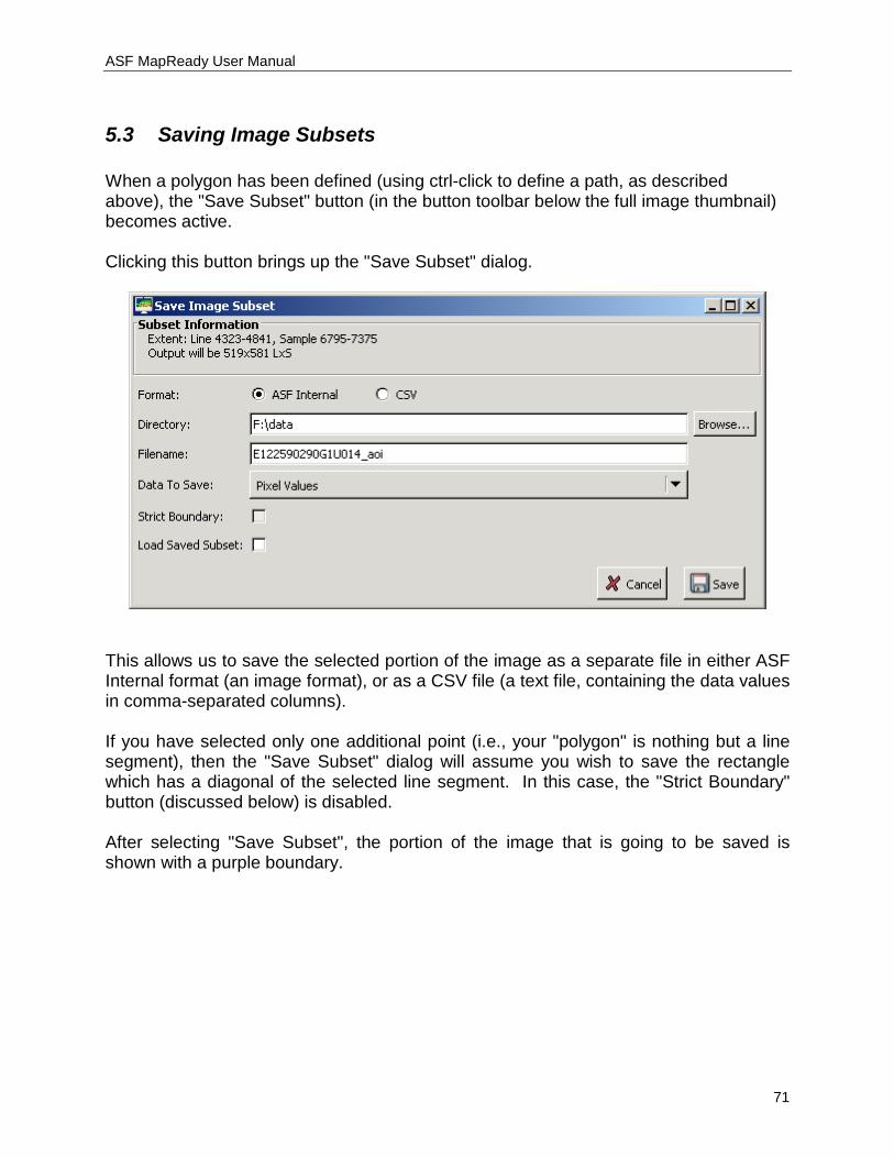
ASF MapReady User Manual
71
5.3 Saving Image Subsets When a polygon has been defined (using ctrl-click to define a path, as described above), the "Save Subset" button (in the button toolbar below the full image thumbnail) becomes active. Clicking this button brings up the "Save Subset" dialog.
This allows us to save the selected portion of the image as a separate file in either ASF Internal format (an image format), or as a CSV file (a text file, containing the data values in comma-separated columns). If you have selected only one additional point (i.e., your "polygon" is nothing but a line segment), then the "Save Subset" dialog will assume you wish to save the rectangle which has a diagonal of the selected line segment. In this case, the "Strict Boundary" button (discussed below) is disabled. After selecting "Save Subset", the portion of the image that is going to be saved is shown with a purple boundary.
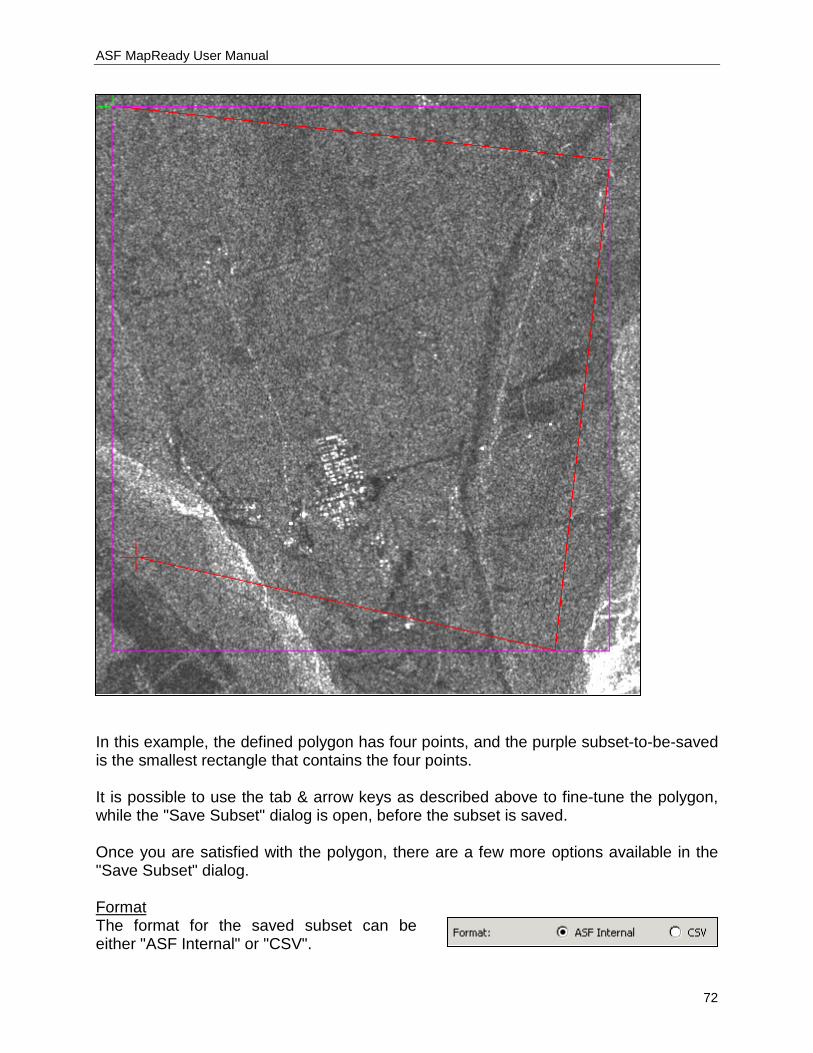
ASF MapReady User Manual
72
In this example, the defined polygon has four points, and the purple subset-to-be-saved is the smallest rectangle that contains the four points. It is possible to use the tab & arrow keys as described above to fine-tune the polygon, while the "Save Subset" dialog is open, before the subset is saved. Once you are satisfied with the polygon, there are a few more options available in the "Save Subset" dialog. FormatThe format for the saved subset can be either "ASF Internal" or "CSV".
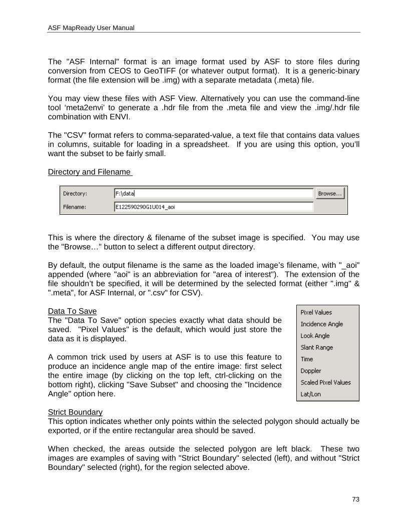
ASF MapReady User Manual
73
The "ASF Internal" format is an image format used by ASF to store files during conversion from CEOS to GeoTIFF (or whatever output format). It is a generic-binary format (the file extension will be .img) with a separate metadata (.meta) file. You may view these files with ASF View. Alternatively you can use the command-line tool ‘meta2envi’ to generate a .hdr file from the .meta file and view the .img/.hdr file combination with ENVI. The "CSV" format refers to comma-separated-value, a text file that contains data values in columns, suitable for loading in a spreadsheet. If you are using this option, you’ll want the subset to be fairly small.
Directory and Filename
This is where the directory & filename of the subset image is specified. You may use the "Browse…" button to select a different output directory. By default, the output filename is the same as the loaded image’s filename, with "_aoi" appended (where "aoi" is an abbreviation for "area of interest"). The extension of the file shouldn’t be specified, it will be determined by the selected format (either ".img" & ".meta", for ASF Internal, or ".csv" for CSV).
The "Data To Save" option species exactly what data should be saved. "Pixel Values" is the default, which would just store the data as it is displayed.
Data To Save
A common trick used by users at ASF is to use this feature to produce an incidence angle map of the entire image: first select the entire image (by clicking on the top left, ctrl-clicking on the bottom right), clicking "Save Subset" and choosing the "Incidence Angle" option here.
This option indicates whether only points within the selected polygon should actually be exported, or if the entire rectangular area should be saved.
Strict Boundary
When checked, the areas outside the selected polygon are left black. These two images are examples of saving with "Strict Boundary" selected (left), and without "Strict Boundary" selected (right), for the region selected above.
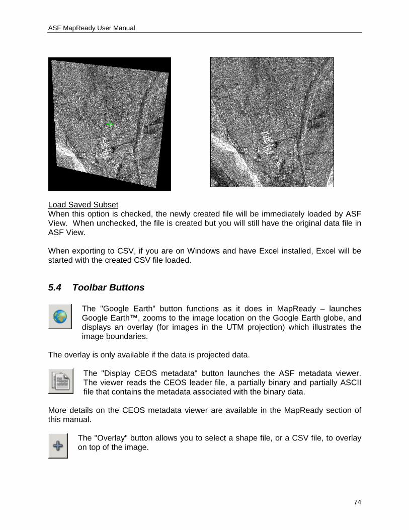
ASF MapReady User Manual
74
When this option is checked, the newly created file will be immediately loaded by ASF View. When unchecked, the file is created but you will still have the original data file in ASF View.
Load Saved Subset
When exporting to CSV, if you are on Windows and have Excel installed, Excel will be started with the created CSV file loaded.
5.4 Toolbar Buttons The "Google Earth" button functions as it does in MapReady – launches Google Earth™, zooms to the image location on the Google Earth globe, and displays an overlay (for images in the UTM projection) which illustrates the image boundaries.
The overlay is only available if the data is projected data.
The "Display CEOS metadata" button launches the ASF metadata viewer. The viewer reads the CEOS leader file, a partially binary and partially ASCII file that contains the metadata associated with the binary data.
More details on the CEOS metadata viewer are available in the MapReady section of this manual.
The "Overlay" button allows you to select a shape file, or a CSV file, to overlay on top of the image.
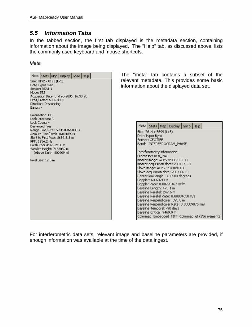
ASF MapReady User Manual
75
5.5 Information Tabs In the tabbed section, the first tab displayed is the metadata section, containing information about the image being displayed. The "Help" tab, as discussed above, lists the commonly used keyboard and mouse shortcuts. Meta
The "meta" tab contains a subset of the relevant metadata. This provides some basic information about the displayed data set.
For interferometric data sets, relevant image and baseline parameters are provided, if enough information was available at the time of the data ingest.

ASF MapReady User Manual
76
Stats The "Stats" tab shows basic image statistics. The values are not exact, since the entire image’s pixel values aren’t used to calculate the values; instead, a subset is used and the statistics are calculated from that. This is to speed up the loading of the image when the application starts. Map
The "Map" tab allows the user to adapt the visualization settings. By default images are displayed with a "Two-Sigma" mapping (data within the range of two standard deviation around the mean value), in order to remove statistical outliers before mapping the image into the visualization range. The "Three-Sigma" option is operating on the same principle, just a wider range. The "Min-Max" option takes the entire value into account, so no values are excluded for the mapping of the values. With the "Truncate" option, no mapping is applied to the data. The "Custom Range" option allows for user defined minimum and maximum values. That way the feature in that particular value range can be enhanced. The "Ignore Values" section of the tab, deals with excluding certain values from the calculation of the statistics. "Ignoring particular value" is most often used for setting a

ASF MapReady User Manual
77
certain background value. The "Ignore range of values" option helps to filter out a bigger value range, e.g. the outliers at the upper value range of an image. Display The "Display" tab contains a few image settings. For multi-band images, such as quad-pol Palsar data, you have the option of combining the bands into a RGB image. By default, the first band is shown in grey-scale, but by selecting the "Combine Bands into RGB" radio button, and selecting bands for each of the RGB channels, a RGB composite image is displayed. When viewing multi-band ALOS images in CEOS format, this multi-band capability is not available – multi-band data spread across multiple files is not supported. You must first import the data, using asf_import (the command-line tool), or MapReady. The "multilook" checkbox is grayed out for images that are already multilooked. No non-multilooked image data types are supported in MapReady 1.0.
The "Apply a Look Up Table" option can be used to convert a grey-scale image to color, using a look up table which maps each grayscale value to RGB values.
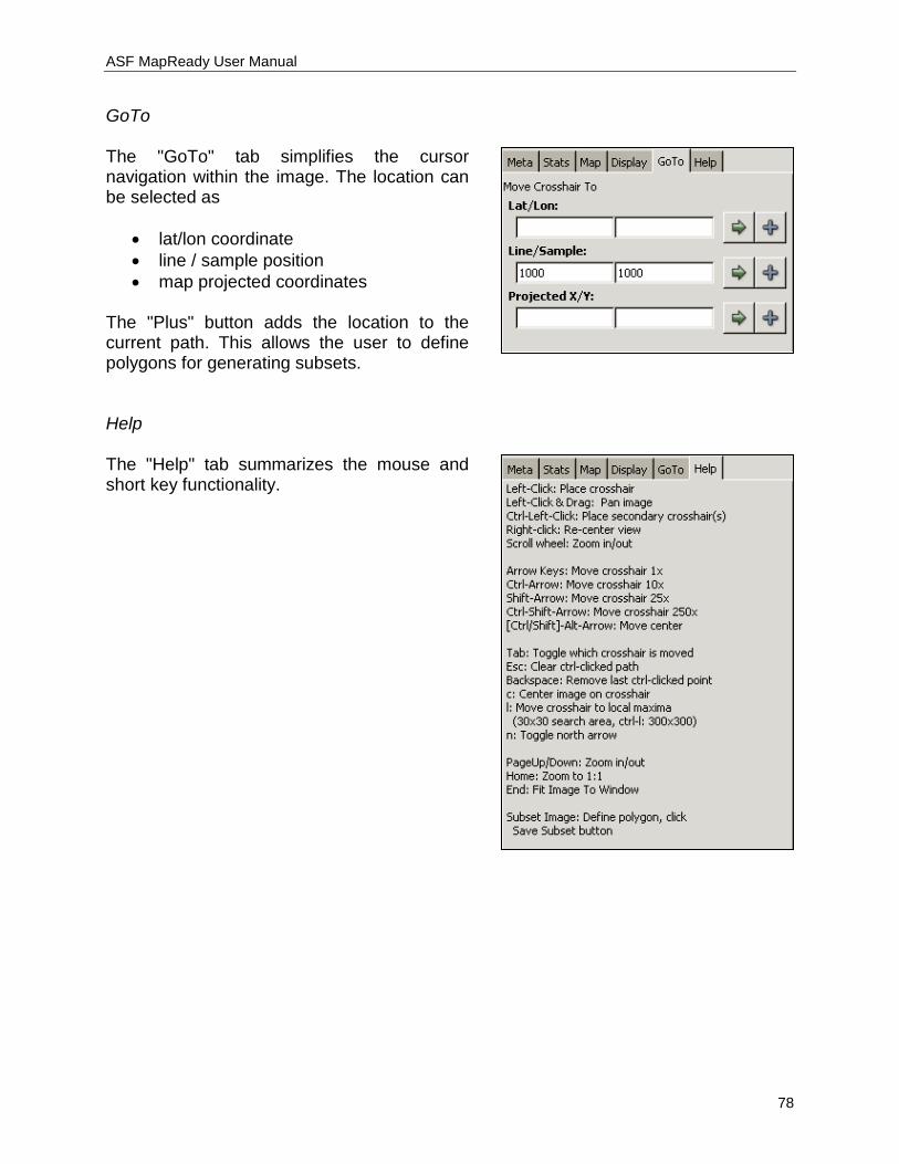
ASF MapReady User Manual
78
GoTo The "GoTo" tab simplifies the cursor navigation within the image. The location can be selected as
• lat/lon coordinate • line / sample position • map projected coordinates
The "Plus" button adds the location to the current path. This allows the user to define polygons for generating subsets. Help The "Help" tab summarizes the mouse and short key functionality.
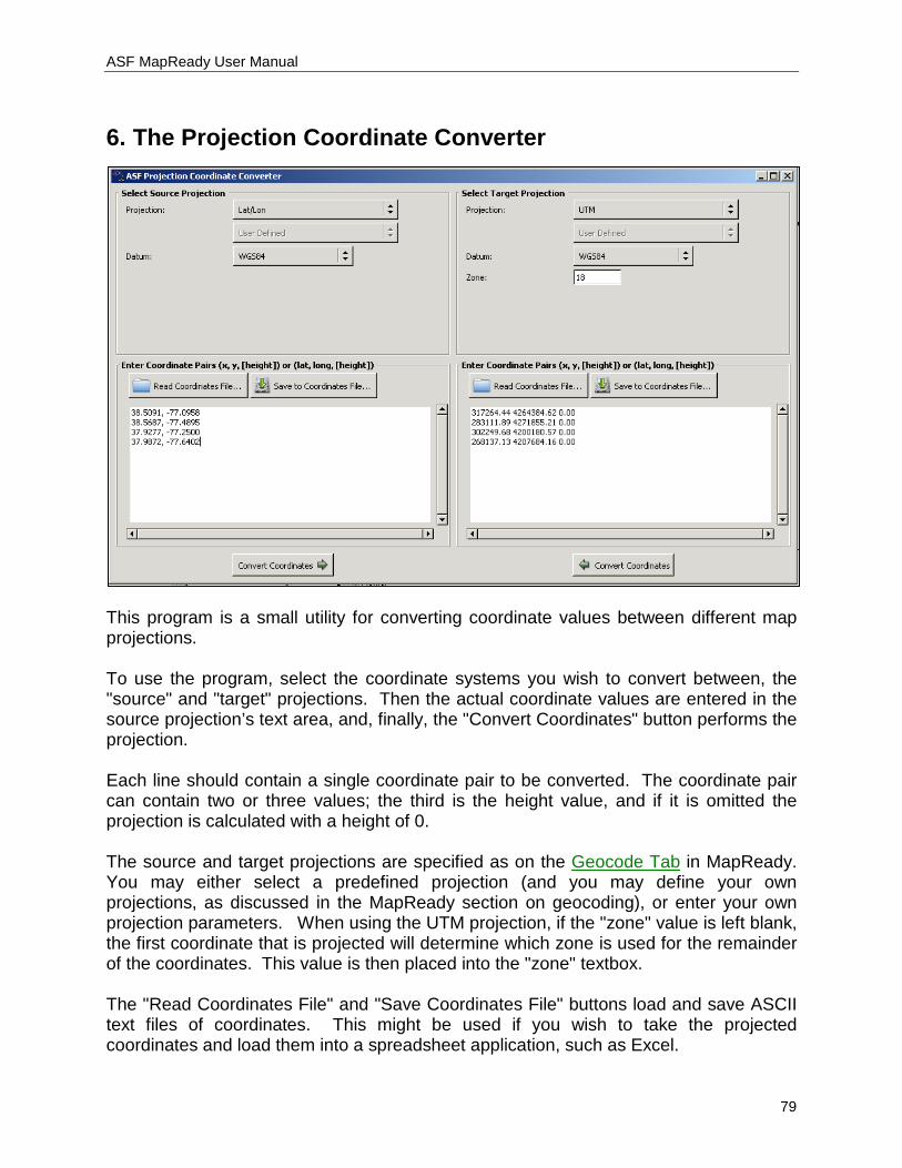
ASF MapReady User Manual
79
6. The Projection Coordinate Converter
This program is a small utility for converting coordinate values between different map projections. To use the program, select the coordinate systems you wish to convert between, the "source" and "target" projections. Then the actual coordinate values are entered in the source projection’s text area, and, finally, the "Convert Coordinates" button performs the projection. Each line should contain a single coordinate pair to be converted. The coordinate pair can contain two or three values; the third is the height value, and if it is omitted the projection is calculated with a height of 0. The source and target projections are specified as on the Geocode Tab in MapReady. You may either select a predefined projection (and you may define your own projections, as discussed in the MapReady section on geocoding), or enter your own projection parameters. When using the UTM projection, if the "zone" value is left blank, the first coordinate that is projected will determine which zone is used for the remainder of the coordinates. This value is then placed into the "zone" textbox. The "Read Coordinates File" and "Save Coordinates File" buttons load and save ASCII text files of coordinates. This might be used if you wish to take the projected coordinates and load them into a spreadsheet application, such as Excel.
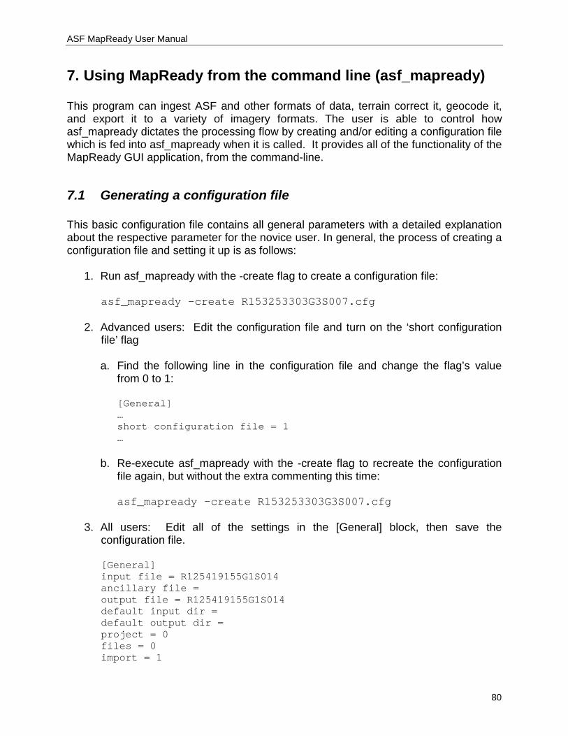
ASF MapReady User Manual
80
7. Using MapReady from the command line (asf_mapready) This program can ingest ASF and other formats of data, terrain correct it, geocode it, and export it to a variety of imagery formats. The user is able to control how asf_mapready dictates the processing flow by creating and/or editing a configuration file which is fed into asf_mapready when it is called. It provides all of the functionality of the MapReady GUI application, from the command-line.
7.1 Generating a configuration file This basic configuration file contains all general parameters with a detailed explanation about the respective parameter for the novice user. In general, the process of creating a configuration file and setting it up is as follows:
1. Run asf_mapready with the -create flag to create a configuration file: asf_mapready –create R153253303G3S007.cfg
2. Advanced users: Edit the configuration file and turn on the ‘short configuration file’ flag
a. Find the following line in the configuration file and change the flag’s value
from 0 to 1: [General] … short configuration file = 1 …
b. Re-execute asf_mapready with the -create flag to recreate the configuration
file again, but without the extra commenting this time:
asf_mapready –create R153253303G3S007.cfg
3. All users: Edit all of the settings in the [General] block, then save the configuration file. [General] input file = R125419155G1S014 ancillary file = output file = R125419155G1S014 default input dir = default output dir = project = 0 files = 0 import = 1
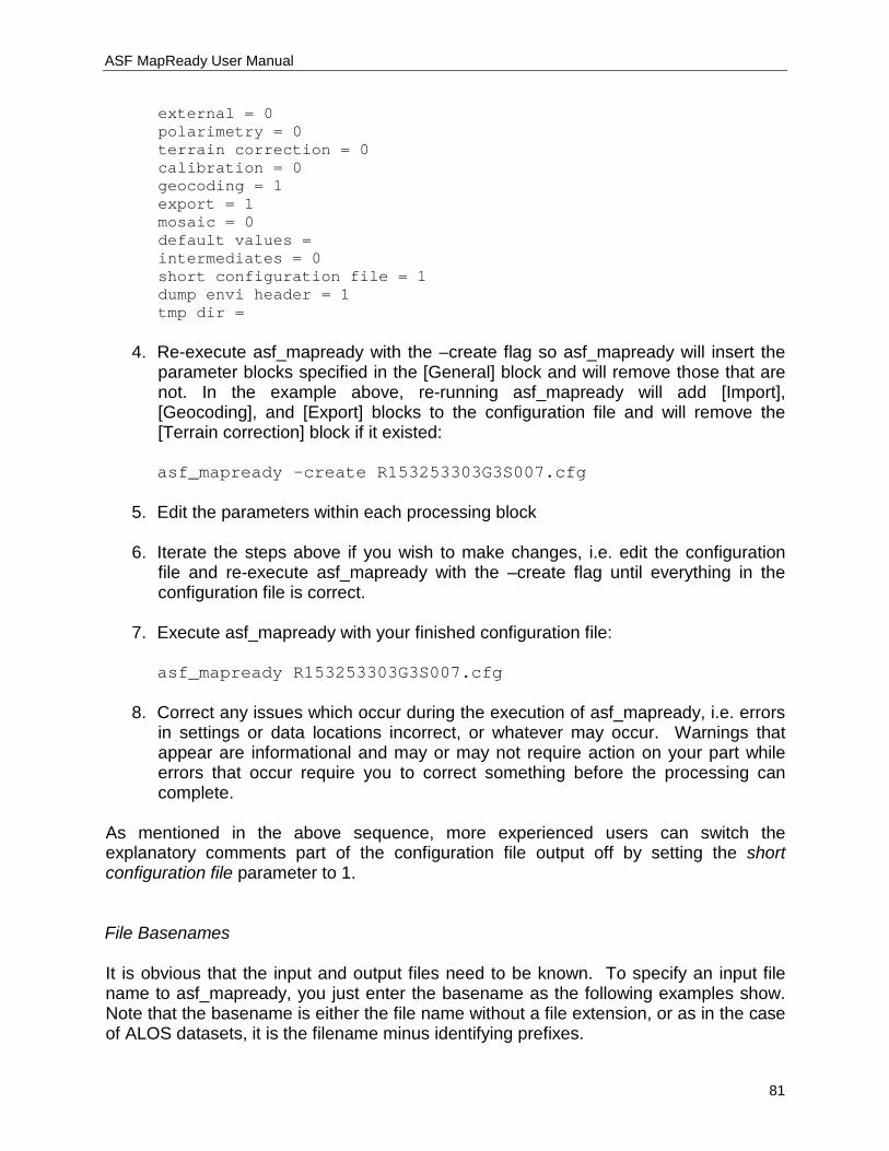
ASF MapReady User Manual
81
external = 0 polarimetry = 0 terrain correction = 0 calibration = 0 geocoding = 1 export = 1 mosaic = 0 default values = intermediates = 0 short configuration file = 1 dump envi header = 1 tmp dir =
4. Re-execute asf_mapready with the –create flag so asf_mapready will insert the parameter blocks specified in the [General] block and will remove those that are not. In the example above, re-running asf_mapready will add [Import], [Geocoding], and [Export] blocks to the configuration file and will remove the [Terrain correction] block if it existed: asf_mapready –create R153253303G3S007.cfg
5. Edit the parameters within each processing block
6. Iterate the steps above if you wish to make changes, i.e. edit the configuration file and re-execute asf_mapready with the –create flag until everything in the configuration file is correct.
7. Execute asf_mapready with your finished configuration file: asf_mapready R153253303G3S007.cfg
8. Correct any issues which occur during the execution of asf_mapready, i.e. errors
in settings or data locations incorrect, or whatever may occur. Warnings that appear are informational and may or may not require action on your part while errors that occur require you to correct something before the processing can complete.
As mentioned in the above sequence, more experienced users can switch the explanatory comments part of the configuration file output off by setting the short configuration file parameter to 1. File Basenames It is obvious that the input and output files need to be known. To specify an input file name to asf_mapready, you just enter the basename as the following examples show. Note that the basename is either the file name without a file extension, or as in the case of ALOS datasets, it is the filename minus identifying prefixes.
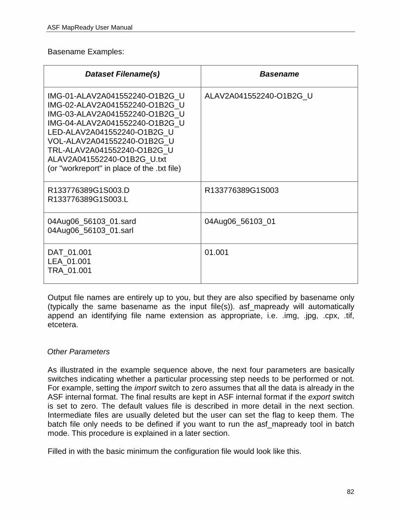
ASF MapReady User Manual
82
Basename Examples:
Dataset Filename(s) Basename
IMG-01-ALAV2A041552240-O1B2G_U IMG-02-ALAV2A041552240-O1B2G_U IMG-03-ALAV2A041552240-O1B2G_U IMG-04-ALAV2A041552240-O1B2G_U LED-ALAV2A041552240-O1B2G_U VOL-ALAV2A041552240-O1B2G_U TRL-ALAV2A041552240-O1B2G_U ALAV2A041552240-O1B2G_U.txt (or "workreport" in place of the .txt file)
ALAV2A041552240-O1B2G_U
R133776389G1S003.D R133776389G1S003.L
R133776389G1S003
04Aug06_56103_01.sard 04Aug06_56103_01.sarl
04Aug06_56103_01
DAT_01.001 LEA_01.001 TRA_01.001
01.001
Output file names are entirely up to you, but they are also specified by basename only (typically the same basename as the input file(s)). asf_mapready will automatically append an identifying file name extension as appropriate, i.e. .img, .jpg, .cpx, .tif, etcetera. Other Parameters As illustrated in the example sequence above, the next four parameters are basically switches indicating whether a particular processing step needs to be performed or not. For example, setting the import switch to zero assumes that all the data is already in the ASF internal format. The final results are kept in ASF internal format if the export switch is set to zero. The default values file is described in more detail in the next section. Intermediate files are usually deleted but the user can set the flag to keep them. The batch file only needs to be defined if you want to run the asf_mapready tool in batch mode. This procedure is explained in a later section. Filled in with the basic minimum the configuration file would look like this.
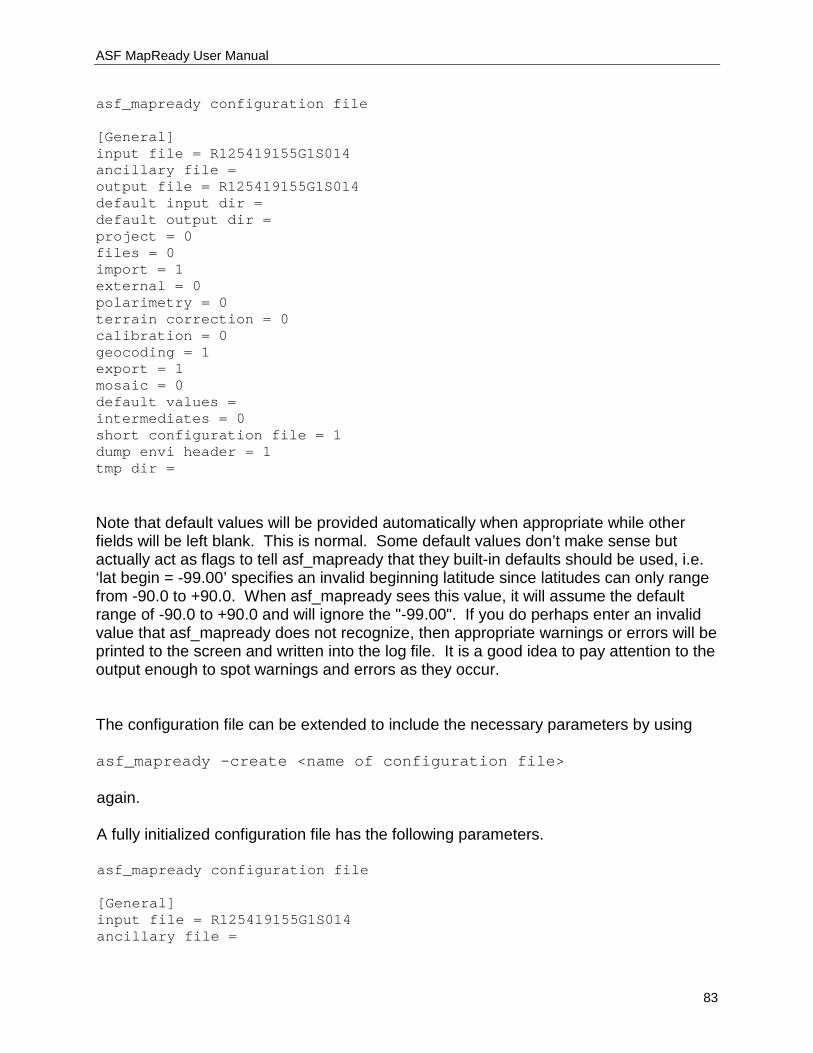
ASF MapReady User Manual
83
asf_mapready configuration file [General] input file = R125419155G1S014 ancillary file = output file = R125419155G1S014 default input dir = default output dir = project = 0 files = 0 import = 1 external = 0 polarimetry = 0 terrain correction = 0 calibration = 0 geocoding = 1 export = 1 mosaic = 0 default values = intermediates = 0 short configuration file = 1 dump envi header = 1 tmp dir = Note that default values will be provided automatically when appropriate while other fields will be left blank. This is normal. Some default values don’t make sense but actually act as flags to tell asf_mapready that they built-in defaults should be used, i.e. ‘lat begin = -99.00’ specifies an invalid beginning latitude since latitudes can only range from -90.0 to +90.0. When asf_mapready sees this value, it will assume the default range of -90.0 to +90.0 and will ignore the "-99.00". If you do perhaps enter an invalid value that asf_mapready does not recognize, then appropriate warnings or errors will be printed to the screen and written into the log file. It is a good idea to pay attention to the output enough to spot warnings and errors as they occur. The configuration file can be extended to include the necessary parameters by using asf_mapready -create <name of configuration file> again. A fully initialized configuration file has the following parameters. asf_mapready configuration file [General] input file = R125419155G1S014 ancillary file =
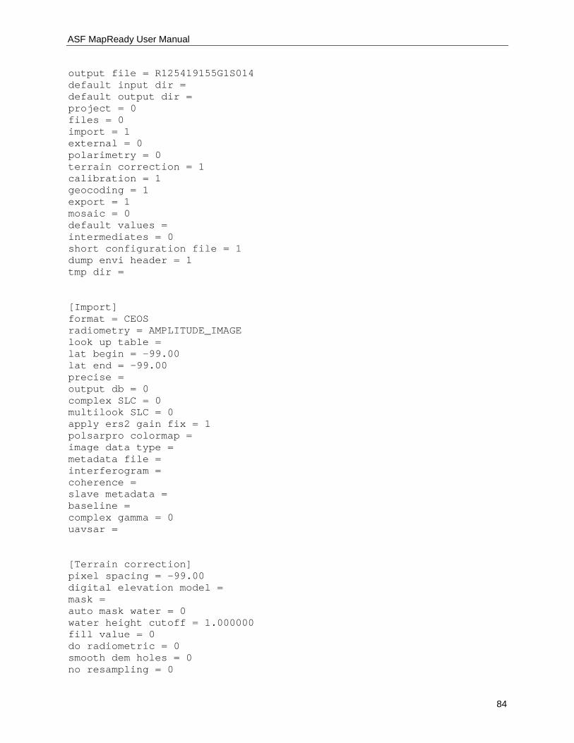
ASF MapReady User Manual
84
output file = R125419155G1S014 default input dir = default output dir = project = 0 files = 0 import = 1 external = 0 polarimetry = 0 terrain correction = 1 calibration = 1 geocoding = 1 export = 1 mosaic = 0 default values = intermediates = 0 short configuration file = 1 dump envi header = 1 tmp dir = [Import] format = CEOS radiometry = AMPLITUDE_IMAGE look up table = lat begin = -99.00 lat end = -99.00 precise = output db = 0 complex SLC = 0 multilook SLC = 0 apply ers2 gain fix = 1 polsarpro colormap = image data type = metadata file = interferogram = coherence = slave metadata = baseline = complex gamma = 0 uavsar = [Terrain correction] pixel spacing = -99.00 digital elevation model = mask = auto mask water = 0 water height cutoff = 1.000000 fill value = 0 do radiometric = 0 smooth dem holes = 0 no resampling = 0
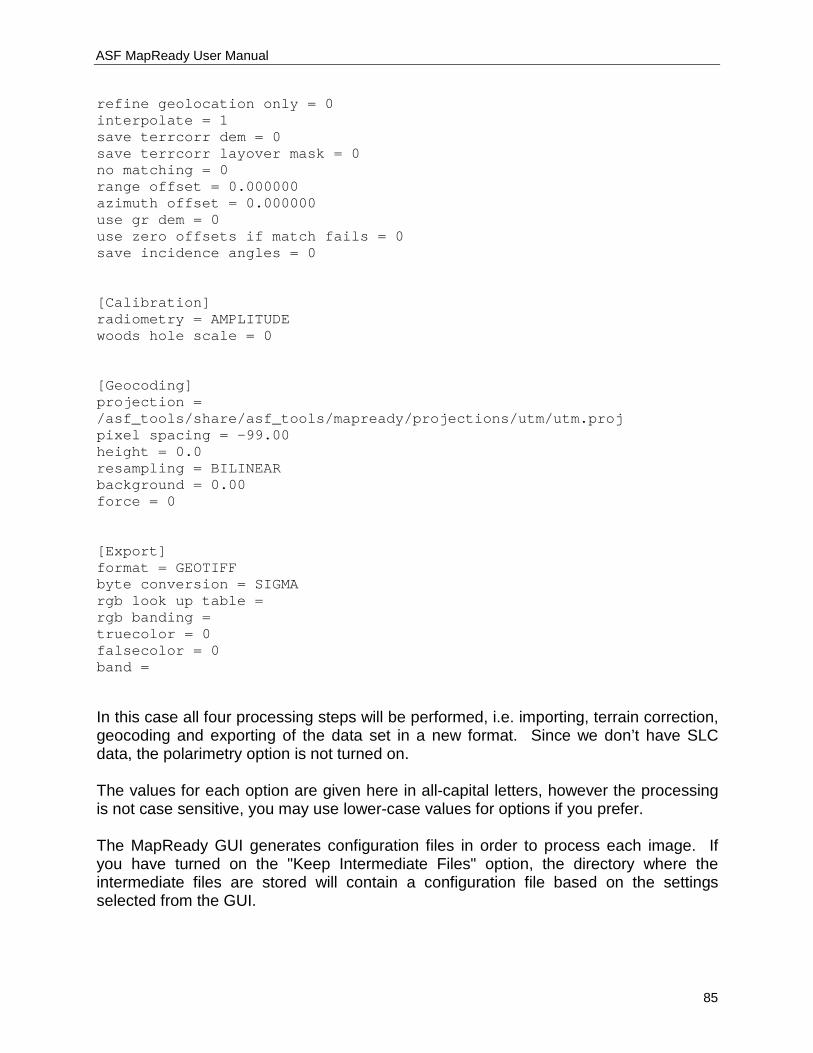
ASF MapReady User Manual
85
refine geolocation only = 0 interpolate = 1 save terrcorr dem = 0 save terrcorr layover mask = 0 no matching = 0 range offset = 0.000000 azimuth offset = 0.000000 use gr dem = 0 use zero offsets if match fails = 0 save incidence angles = 0 [Calibration] radiometry = AMPLITUDE woods hole scale = 0 [Geocoding] projection = /asf_tools/share/asf_tools/mapready/projections/utm/utm.proj pixel spacing = -99.00 height = 0.0 resampling = BILINEAR background = 0.00 force = 0 [Export] format = GEOTIFF byte conversion = SIGMA rgb look up table = rgb banding = truecolor = 0 falsecolor = 0 band =
In this case all four processing steps will be performed, i.e. importing, terrain correction, geocoding and exporting of the data set in a new format. Since we don’t have SLC data, the polarimetry option is not turned on. The values for each option are given here in all-capital letters, however the processing is not case sensitive, you may use lower-case values for options if you prefer. The MapReady GUI generates configuration files in order to process each image. If you have turned on the "Keep Intermediate Files" option, the directory where the intermediate files are stored will contain a configuration file based on the settings selected from the GUI.
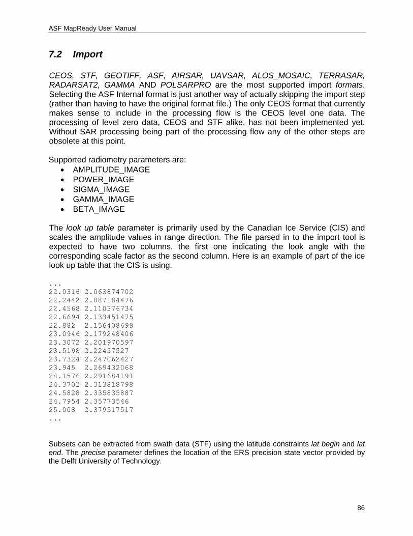
ASF MapReady User Manual
86
7.2 Import CEOS, STF, GEOTIFF, ASF, AIRSAR, UAVSAR, ALOS_MOSAIC, TERRASAR, RADARSAT2, GAMMA AND POLSARPRO are the most supported import formats. Selecting the ASF Internal format is just another way of actually skipping the import step (rather than having to have the original format file.) The only CEOS format that currently makes sense to include in the processing flow is the CEOS level one data. The processing of level zero data, CEOS and STF alike, has not been implemented yet. Without SAR processing being part of the processing flow any of the other steps are obsolete at this point. Supported radiometry parameters are:
• AMPLITUDE_IMAGE • POWER_IMAGE • SIGMA_IMAGE • GAMMA_IMAGE • BETA_IMAGE
The look up table parameter is primarily used by the Canadian Ice Service (CIS) and scales the amplitude values in range direction. The file parsed in to the import tool is expected to have two columns, the first one indicating the look angle with the corresponding scale factor as the second column. Here is an example of part of the ice look up table that the CIS is using. ... 22.0316 2.063874702 22.2442 2.087184476 22.4568 2.110376734 22.6694 2.133451475 22.882 2.156408699 23.0946 2.179248406 23.3072 2.201970597 23.5198 2.22457527 23.7324 2.247062427 23.945 2.269432068 24.1576 2.291684191 24.3702 2.313818798 24.5828 2.335835887 24.7954 2.35773546 25.008 2.379517517 ... Subsets can be extracted from swath data (STF) using the latitude constraints lat begin and lat end. The precise parameter defines the location of the ERS precision state vector provided by the Delft University of Technology.
ASF MapReady User Manual
87
When the calibration parameters are applied to the data during the import, the resulting values are in power scale. The output db parameter changes this behavior and the values in the output image are stored in dB. Single look complex (SLC) can be dealt with in various ways. By default, the data will be ingested as a two-band image, an amplitude band and a phase band. Alternatively, the data can be kept in its original format, having a real and imaginary part, by setting the complex SLC flag. Unless the complex data is used for polarimetric processing, the data can be safely multilooked setting the multilook SLC flag to 1. The power in ERS-2 data decreased over time. The apply ers2 gain fix flag (default value) adjusts the brightness as a function of time.
7.3 Polarimetry The polarimetric processing requires quad-pol SLC data. This part of the processing flow is currently only working ALOS Palsar data. There are number of decompositions and classification supported. Three common polarimetric decompositions supported by MapReady. Setting the respective flags (pauli, sinclair and freeman durden) will include them in the processing flow. The Cloude-Pottier classification can be run in two different ways. The cloude pottier flag maps the results to eight classes, whereas the extended cloude pottier flag results in sixteen classes. Both classifications are based on entropy, anisotropy and alpha values. These can be stored as three separate bands using the entropy anisotropy alpha flag. Atmospheric conditions that rotate the polarity of the SAR signal can be corrected using the Faraday correction. In addition, a farcorr threshold can be set that only corrects the data for Faraday rotation when this threshold is exceeded.
7.4 Terrain correction For the terrain correction portion of the processing a digital elevation model (see also How to guide – Digital elevation models) is required. If the SAR image and the reference DEM have different pixel spacing the resolution of terrain corrected SAR image needs to be adjusted. This resampling can be left to the asf_mapready tool to determine by setting the pixel spacing to -99.0 in the configuration file. This is the default setting. Alternatively, a user defined value can be set instead.
ASF MapReady User Manual
88
The digital elevation model parameter defines the location of the reference DEM. During the terrain correction process, co-registration of the DEM and SAR image is accomplished in SAR geometry. In some cases, when parts of the images are known to be moving or changing (e.g. water, glaciers etc.), this can confuse the co-registration step and cause it to fail. If you provide the terrain correction step with a mask file that defines areas of the image to ignore, i.e. the water or glacial regions, then the co-registration step has a far higher likelihood of success. Instead of creating a mask manually (see How to guide – Generating a mask for terrain correction), you may allow the terrain correction processing to automatically generate a mask for you by setting the auto mask water flag. The automatically-generated mask is based on the DEM and attempts to mask the regions of your scene that are water (those regions which may result in a poor match). Specifically, all DEM height values of less than 1 meter are masked out. You may instead force the automatically created mask to mask out all terrain below some other height by specifying a different water height cutoff in the terrain correction block of the configuration file. When applying a mask during terrain correction, you can choose how the regions covered by the mask are filled-in in the final terrain corrected result. If you would like the SAR data to be kept then use -1 as the fill value, otherwise enter a value that you’d like to use instead. The terrain correction is applying a geometric correction to the data. In addition to that the data can be radiometrically corrected for the effects of the local incidence angle. For this the do radiometric flag needs to be set. Digital elevation models acquired by the Shuttle Radar Topography Mission (SRTM) have holes in identified problem areas. This can cause some streaking in the terrain corrected product. Setting the smooth dem holes parameter replaces the DEM holes with interpolated values. The terrain correction is down sampling the DEM if it is significantly larger than the SAR image. This behavior can be overruled by setting the no resampling parameter. When applying terrain correction to low-topography (flat) regions, the results may not be entirely accurate. In these cases, the reference DEM might still be used to improve the geolocation of the SAR image without performing the actual terrain correction. This can be achieved by setting the refine geolocation only flag. With this option, the image data is not changed at all – only the geolocation information in the metadata is affected. Layover and shadow regions are problem areas in images that are in the original SAR geometry since the backscatter information is either heavily condensed or missing. In the terrain correction process they can either be left black (resulting in better image statistics in the remainder of the image) or they may be interpolated over (resulting in a
ASF MapReady User Manual
89
nicer-looking image). Setting the interpolate parameter to 1 indicates that these regions should be interpolated over. For a more detailed analysis of the terrain correction results a couple of files used in the process can be saved. Setting the save terrcorr dem parameter keeps the clipped (to the SAR image extents) reference DEM in slant range geometry. Setting the save terrcorr layover mask parameter keeps the layover and shadow mask. There are few parameters that can be set to overwrite the standard matching procedure that is carried out during the terrain correction. The no matching parameter eliminates the processing step that applies the offsets that the program determined between the real and a simulated SAR image. Using the range offset and azimuth offset parameters overwrites the results from this matching step.
7.5 Geocoding The geocoding tool currently supports five different map projections: Universal Transverse Mercator (UTM), Polar Stereographic, Albers Equal Area Conical, Lambert Conformal Conical and Lambert Azimuthal Equal Area. For all these map projections a large number of projection parameter files have been predefined for various parts of the world. The projection parameter in the geocoding block indicates the file name of the predefined projection parameter file. Users can define their projection parameter file using the text editor of their choice. On Unix systems the projection parameter files are located in the asf_tools/share/asf_tools/projections/<projection> directories, while on Windows systems they are located in the projections/<projection> directories in the ASF Tools installation folder, by default this is c:\Program Files\ASF_Tools. The projection parameter file for the UTM projection is a special case. It contains an empty zone parameter, in which case asf_geocode determines the zone from the center longitude of the image. It allows the use of any other zone for the geocoding as long as that zone is covered in the imagery. For these cases the user can define the zone parameter in the generic UTM projection file. The pixel spacing determines the pixel size used for the resulting geocoded image and, therefore, the size of the output image. The default setting of -99.0 results in no change in pixel size during the geocoding process. An average height can be defined for the image that is taken into account and adjusted for during the geocoding process. The default height is set to 0.0 meters (no height correction.) Furthermore, a vertical datum can be defined for geocoded image. WGS84, NAD27 and NAD83 comprise the list of supported datums. In addition, a Hughes reference spheroid may be specified for the datum parameter as well.
ASF MapReady User Manual
90
Three different resampling methods have been implemented as part of the geocoding: NEAREST NEIGHBOR, BILINEAR and BICUBIC. The bilinear resampling method is the default. After geocoding, a fill value is required for the regions outside the geocoded image. By default this value is 0, but may be set to a different value here. In order to ensure the proper use of projection parameter files, we have implemented a number of checks that verify whether the map projection parameters are reasonable for the area that is covered by the data. For example, applying a projection parameter file that is defined for South America for a data set that is covering Alaska would lead to huge distortions. These checks can be overridden by setting the force option.
7.6 Export The following format values are considered valid:
• TIFF • GEOTIFF • JPEG • PGM • PNG • POLSARPRO
All formats, with the exception of GeoTIFF, require the scaling of the internal ASF (usually 32-bit floating point) format from to byte format. The GeoTIFF supports byte as well as floating point data. The byte conversion options are SIGMA, MINMAX, TRUNCATE or HISTOGRAM_EQUALIZE. They scale the floating point values to byte values in various ways:
• SIGMA – Determines the mean and standard deviation of an image, calculates a two sigma (i.e., standard deviations) range around the mean value, and then maps image values within this range to 0 to 255. Image values that map to below 0 using are set to 0, and image values that map to greater than 255 are set to 255.
• MINMAX – Determines the minimum and maximum values of the input image and linearly maps those values to the byte range of 0 to 255.
• TRUNCATE – Values less than 0.0 are mapped to 0, values greater than 255.0 are mapped to 255, and values in between have their fractional portions truncated, i.e., 29.7 would become 29 exactly.
• HISTOGRAM_EQUALIZE – Histogram equalization is designed to optimize viewing for humans. It is a nonlinear contrast enhancement that expands low-dynamic range regions over a broader range of values and at the same time compresses areas of higher dynamic range over a lesser range of values. The

ASF MapReady User Manual
91
remapping function is derived from the image histogram. Histogram equalization is useful for bringing out detail in areas of the image that otherwise seem to lack detail due to ‘flatness’ or ‘sameness’ in the brightness values, i.e. in dark or light regions or regions of similarly-grey values. Because this transform is nonlinear however, very small changes in the geolocation of may occur. The amount of change is not predictable and is completely dependent on the distribution of the data values in the image, but should be quite small, i.e. fractions of a pixel to a pixel in magnitude (est.).
7.7 Default values file The default values file specified in the [General] block (in the configuration file) is used to define the user's preferred parameter settings. In most cases, you will work on a study where your area of interest is geographically well defined. You want the data for the entire project in the same projection, with the same pixel spacing and the same output format. The default values file is essential part of the batch processing, described in the next section. Here is an example of a default values file that the Canadian Ice Service (CIS) is using for their automated processing system. import = 1 sar processing = 0 geocoding = 1 export = 1 terrain correction = 0 background = 0 intermediates = 0 quiet = 0 short configuration file = 0 input format = CEOS radiometry = AMPLITUDE_IMAGE look up table = /export/cis/cis_ice.lut projection = /export/asf_tools/share/projections/utm/utm.proj pixel spacing = 100 height = 0.0 datum = WGS84 resampling = BILINEAR force = 0 output format = GEOTIFF byte conversion = SIGMA smooth dem holes = 1
Note that it is not necessary, in a default settings file, to group the settings into blocks as in the normal configuration file. The block names are there to categorize the settings for reasons of clarity. All of the individual settings themselves are unique in their
ASF MapReady User Manual
92
naming to prevent ambiguity. The easiest way to create a default settings file, which is nothing but a simple text file and can use any naming that you desire, is to use asf_mapready with the –create flag to create a configuration file first. Then edit that file and use it as a default settings file. It is important to understand the order of events that occur as asf_mapready reads and uses both the configuration file created with the –create flag as well as the default settings file that default values field refers to. Here is how asf_mapready utilizes the settings in these two files:
1. asf_mapready reads the normal configuration file to determine the path and name of the default settings file.
2. asf_mapready then reads the default settings file as though it were a normal configuration file
3. asf_mapready then re-reads the normal configuration file and allows settings from that file to override the defaults found in the default settings file
4. Processing then continues according to the final combination of settings Perhaps the best way to utilize the default settings file is to use one (or more) together with a standard configuration file that has had similar entries removed, i.e. define geocoding (map projection) parameters in the default settings file but delete the [Geocoding] block and its parameters found in the regular configuration file. Note that if you take this approach, that you would still (for this example) leave the geocoding flag in the [General] block of the normal configuration file set to ‘1’. The difference is that the appropriate parameters will be found in the default settings file instead. If you perchance ran asf_mapready with the –create flag again however, then the [Geocoding] block would be automatically added back to your configuration file. Take a look at a configuration file and at the default settings file provided by the ASF and experiment a bit to clarify how things work. You can find the default settings file provided by the ASF in the asf_mapready subfolder of your share directory (located where previously mentioned in this document.)
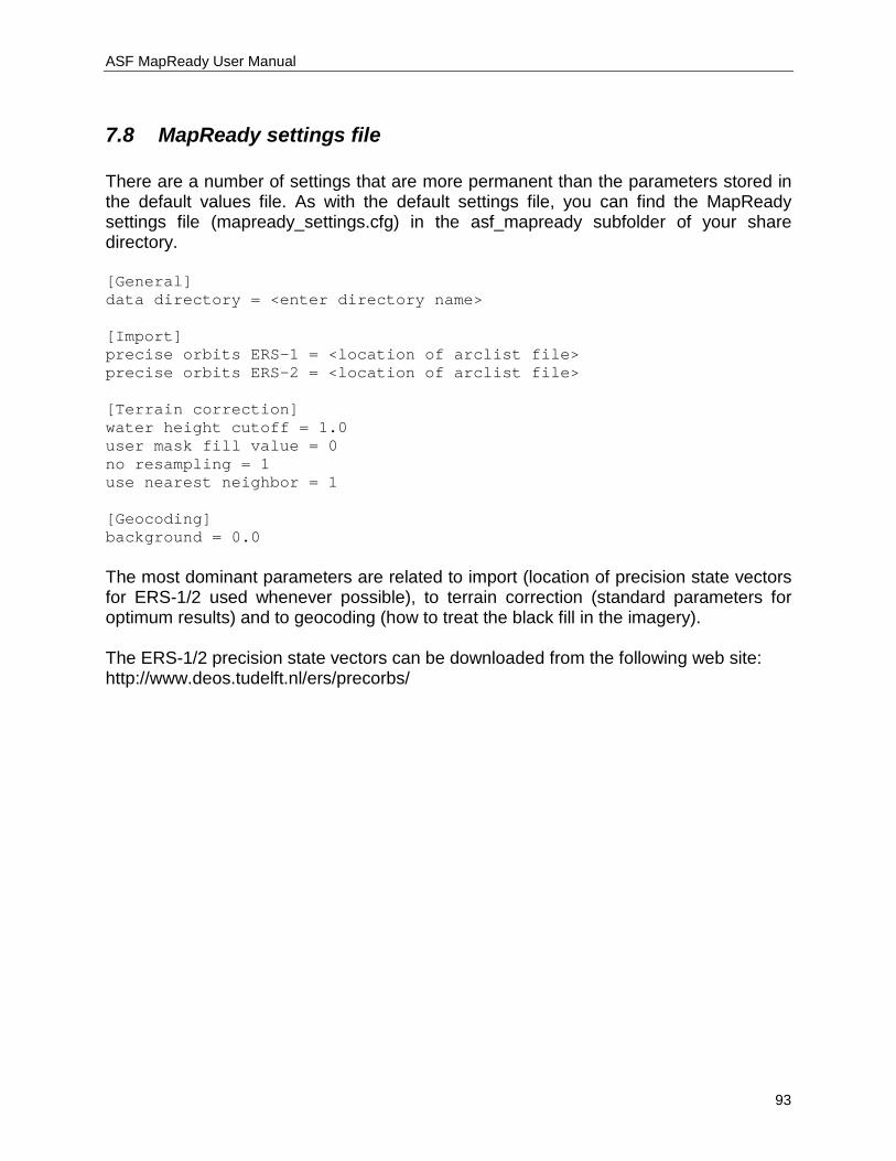
ASF MapReady User Manual
93
7.8 MapReady settings file There are a number of settings that are more permanent than the parameters stored in the default values file. As with the default settings file, you can find the MapReady settings file (mapready_settings.cfg) in the asf_mapready subfolder of your share directory. [General] data directory = <enter directory name> [Import] precise orbits ERS-1 = <location of arclist file> precise orbits ERS-2 = <location of arclist file> [Terrain correction] water height cutoff = 1.0 user mask fill value = 0 no resampling = 1 use nearest neighbor = 1 [Geocoding] background = 0.0 The most dominant parameters are related to import (location of precision state vectors for ERS-1/2 used whenever possible), to terrain correction (standard parameters for optimum results) and to geocoding (how to treat the black fill in the imagery). The ERS-1/2 precision state vectors can be downloaded from the following web site: http://www.deos.tudelft.nl/ers/precorbs/
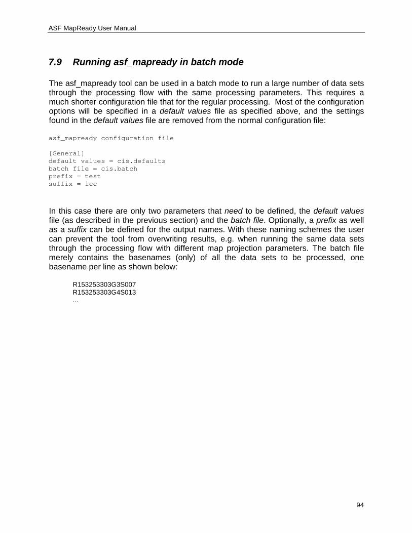
ASF MapReady User Manual
94
7.9 Running asf_mapready in batch mode The asf_mapready tool can be used in a batch mode to run a large number of data sets through the processing flow with the same processing parameters. This requires a much shorter configuration file that for the regular processing. Most of the configuration options will be specified in a default values file as specified above, and the settings found in the default values file are removed from the normal configuration file: asf_mapready configuration file [General] default values = cis.defaults batch file = cis.batch prefix = test suffix = lcc In this case there are only two parameters that need to be defined, the default values file (as described in the previous section) and the batch file. Optionally, a prefix as well as a suffix can be defined for the output names. With these naming schemes the user can prevent the tool from overwriting results, e.g. when running the same data sets through the processing flow with different map projection parameters. The batch file merely contains the basenames (only) of all the data sets to be processed, one basename per line as shown below:
R153253303G3S007 R153253303G4S013 ...
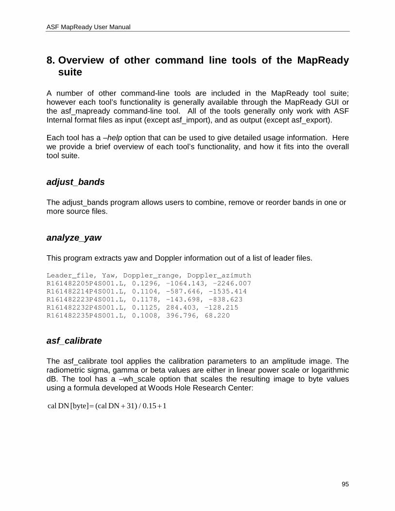
ASF MapReady User Manual
95
8. Overview of other command line tools of the MapReady suite
A number of other command-line tools are included in the MapReady tool suite; however each tool’s functionality is generally available through the MapReady GUI or the asf_mapready command-line tool. All of the tools generally only work with ASF Internal format files as input (except asf_import), and as output (except asf_export). Each tool has a –help option that can be used to give detailed usage information. Here we provide a brief overview of each tool’s functionality, and how it fits into the overall tool suite.
adjust_bands The adjust_bands program allows users to combine, remove or reorder bands in one or more source files.
analyze_yaw This program extracts yaw and Doppler information out of a list of leader files. Leader_file, Yaw, Doppler_range, Doppler_azimuth R161482205P4S001.L, 0.1296, -1064.143, -2246.007 R161482214P4S001.L, 0.1104, -587.646, -1535.414 R161482223P4S001.L, 0.1178, -143.698, -838.623 R161482232P4S001.L, 0.1125, 284.403, -128.215 R161482235P4S001.L, 0.1008, 396.796, 68.220
asf_calibrate The asf_calibrate tool applies the calibration parameters to an amplitude image. The radiometric sigma, gamma or beta values are either in linear power scale or logarithmic dB. The tool has a –wh_scale option that scales the resulting image to byte values using a formula developed at Woods Hole Research Center:
1 0.15/ 31) DN (cal [byte] DN cal ++=
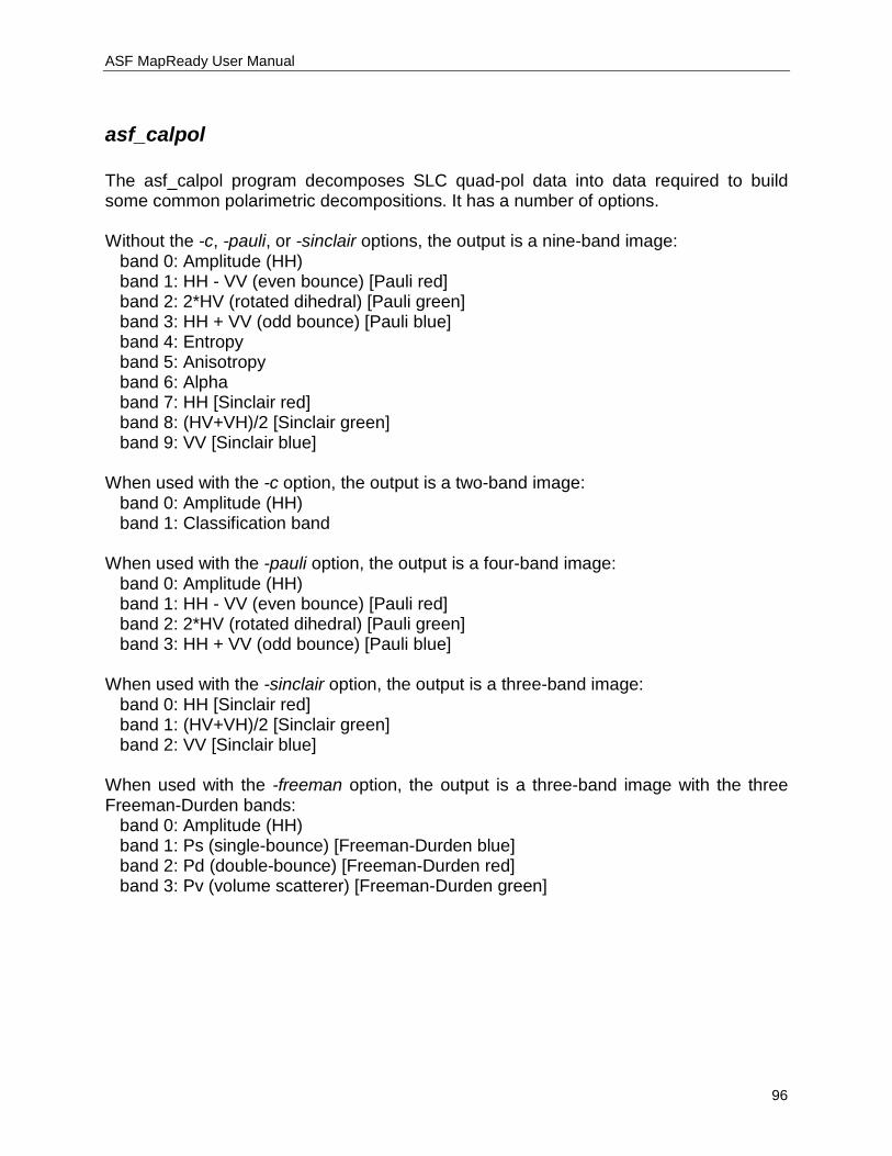
ASF MapReady User Manual
96
asf_calpol The asf_calpol program decomposes SLC quad-pol data into data required to build some common polarimetric decompositions. It has a number of options. Without the -c, -pauli, or -sinclair options, the output is a nine-band image: band 0: Amplitude (HH) band 1: HH - VV (even bounce) [Pauli red] band 2: 2*HV (rotated dihedral) [Pauli green] band 3: HH + VV (odd bounce) [Pauli blue] band 4: Entropy band 5: Anisotropy band 6: Alpha band 7: HH [Sinclair red] band 8: (HV+VH)/2 [Sinclair green] band 9: VV [Sinclair blue] When used with the -c option, the output is a two-band image: band 0: Amplitude (HH) band 1: Classification band When used with the -pauli option, the output is a four-band image: band 0: Amplitude (HH) band 1: HH - VV (even bounce) [Pauli red] band 2: 2*HV (rotated dihedral) [Pauli green] band 3: HH + VV (odd bounce) [Pauli blue] When used with the -sinclair option, the output is a three-band image: band 0: HH [Sinclair red] band 1: (HV+VH)/2 [Sinclair green] band 2: VV [Sinclair blue] When used with the -freeman option, the output is a three-band image with the three Freeman-Durden bands: band 0: Amplitude (HH) band 1: Ps (single-bounce) [Freeman-Durden blue] band 2: Pd (double-bounce) [Freeman-Durden red] band 3: Pv (volume scatterer) [Freeman-Durden green]
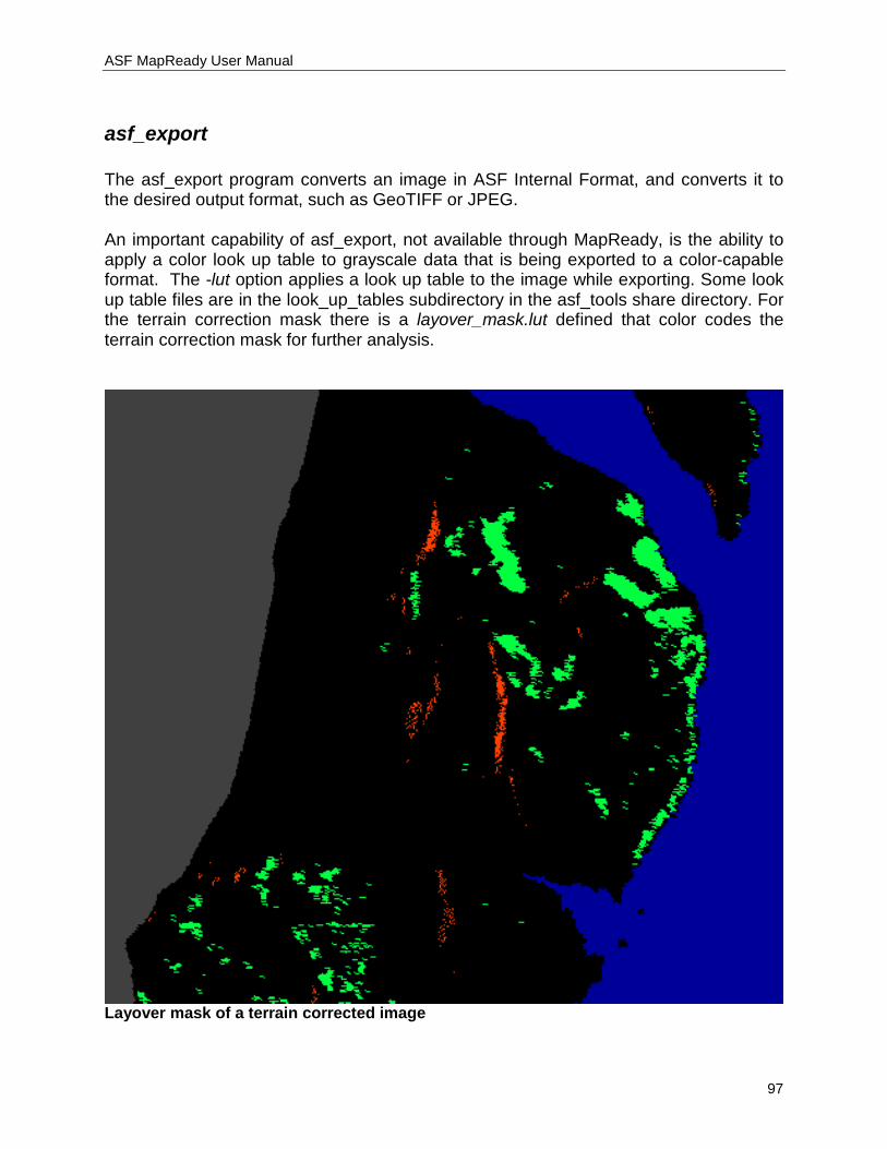
ASF MapReady User Manual
97
asf_export The asf_export program converts an image in ASF Internal Format, and converts it to the desired output format, such as GeoTIFF or JPEG. An important capability of asf_export, not available through MapReady, is the ability to apply a color look up table to grayscale data that is being exported to a color-capable format. The -lut option applies a look up table to the image while exporting. Some look up table files are in the look_up_tables subdirectory in the asf_tools share directory. For the terrain correction mask there is a layover_mask.lut defined that color codes the terrain correction mask for further analysis.
Layover mask of a terrain corrected image
ASF MapReady User Manual
98
asf_geocode The program asf_geocode takes a map projected or, more commonly, an unprojected (e.g., a ground range) image and geocodes it, i.e., maps it to a specified map projection, such as UTM or Polar Stereographic. The geocoding process works by first mapping the edges of the original image into the output coordinate system, and from those finding the extents of the input image in the output projection space. Then, each pixel in the output is reverse-mapped to find its corresponding pixel in the input coordinate system, which is then placed in the output image. Since the output pixel will not typically correspond exactly with a single pixel in the input image, resampling or interpolating must be performed. This utility performs the functionality available on the "Geocode" tab of MapReady, and the [Geocode] section of asf_mapready.
asf_import The asf_import tool is used to ‘import’ data from its original format to the internal format used by the ASF tools (MapReady package, the SAR Training Processor, etc). This program must be used on any data before any of the other command line tools can be used with that data. The antenna pattern can be applied to SAR data by using the -sigma, -beta, or -gamma options (the antenna calibration coefficients are included in the CEOS metadata). Doing so will apply the antenna pattern to the data in the given β0, γ0 or σ0 projection. The product will be in the power scale. If it is preferred to have the data in the decibel scale, the -db flag can be used. Complex SLC data are can be processed in a variety of ways. By default, asf_import will generate two bands, an amplitude band and a phase band, out of every SLC input that it encounters. This allows the user to visualize those data sets at any time. The -complex option leaves the SLC in its original complex form, storing it in its real and imaginary part. In case the user is not interested in polarimetric processing, it is advisable to use the -multilook option to generate an output image with square pixel size. That can significantly reduce the data volume and the result can be interpreted in a more straightforward way. A more refined multilooking can be achieved by using the –azimuth-look-count and –range-look-count options. These options allow the definition of any ratio to applied to the data instead the default one. For multiband images there is a -band option to ingest individual bands. GeoTIFF files do not provide any information about the type of data they contain. The -image_data_type option allows the user to specify the type of data. The most useful image data types are 'amplitude_image', 'phase_image', 'coherence_image',
ASF MapReady User Manual
99
'lut_image', 'elevation', 'dem', 'polarimetric_image', 'image', 'image_layer_stack' and 'mask'.
asf_kml_overlay The asf_kml_overlay tool generates KML overlays from a large variety of ASF internal and PolSARPro files. The tool verifies that the data is actually geocoded to one of the map projections supported by the ASF tools. In order to ensure a better alignment within Google Earth™, it is advisable to use a digital elevation model to terrain correct or to refine the geolocation of the input image. As a first processing the input image is re-projected into the equi-rectangular map projection that is internally used by Google Earth™. The properties of the resulting PNG file are mostly defined by two options: –reduction_factor and –transparency. The reduction factor is multiplied by the pixel size to reduce the size of the image (default value: 8). The transparency value defines the level of transparency of the overlay (value range of 0 to 100 with default value of 0). There are two ways of generating color overlays. For single-band images a color look up table (LUT) can be applied with the –colormap option. For this purpose the user can provide his own LUTs or take advantage of the predefined LUTs in the share directory. For multi-band imagery the –rgb option allows the user to refine bands for the red, green and blue channels. There are three types of KML overlays that are specifically generated for PolSARPro files: segmentation, decomposition and parameter. They are defined with –polsarpro option.
asf_mapready The asf_mapready program is command line version of what is behind the MapReady GUI. It allows the user to run larger amounts of data without any manual interaction. The only input the tool needs is a configuration file that defines all the processing parameters. It is described in more detail in a previous section.
asf_proj2proj This is a command-line interface to the ASF Projection Coordinate Converter. To use it, you must have the source and target projections defined in projection files, though one of them may be the "latlon" pseudo projection. Projection files are generated by MapReady during geocoding, if you’ve saved your temporary files one will have been created and placed in the temporary directory. Also,
ASF MapReady User Manual
100
the predefined projections used by MapReady and the Projection Coordinate Converter located in the "projections" folder in the MapReady installation directory can be used.
asf_terrcorr The asf_terrcorr program terrain corrects or ‘orthorectifies’ the SAR data from its original side looking time based geometry (radar) to an orthogonal nadir view so that it aligns nicely with photographic images. It takes a SAR image and a digital elevation model (DEM) as input. A simulated SAR image is created based on the DEM using the satellite’s oribit information (state vectors). The SAR and simulated SAR are then corregistered (matched). Based on that coregistration the values of each of the SAR pixels are ‘painted’ in the location of the corresponding pixel of the original DEM. This utility performs the functionality availabe in the "Terrain Correction" tab of MapReady, and the [Terrain correction] section of asf_mapready.
asf_view This tool is described in more detail in a previous section.
brs2jpg The brs2jpg tool converts ALOS Palsar browse images (.BRS), located in the BROWSE directory of the respective data product, into JPEG format. The information about the browse image dimensions is stored in the workreport file that is required as an input file.
combine This program mosaics the input files together, producing an output image that is the union of all listed input images. Where the input images overlap, the pixel in the image listed earlier on the command-line is chosen. At least two input files are required. You may list as many input files as desired, however extremely large output files will take some time to process. All input files must be geocoded to the same projection, with the same projection parameters, and the same pixel size.
deskew Deskew is used by terrain correction to ‘square up’ an image for co-registration once it has been converted to slant range. It uses the squint angle of an image along with the
ASF MapReady User Manual
101
look angle to determine the amount of parallelogram shift skew that has been introduced in an image due to the Doppler centroid chosen during image processing. It then remaps the image (using bilinear interpolation) to remove this.
diffimage Diffimage is an image analysis tool for comparing two images. The tool calculates image statistics within each input image and calculates the peak signal-to-noise (PSNR) between the two images. It also verifies any shifts between the two images. The image statistics and shifts are the basis for determining whether the images are different or not.
diffmeta Diffmeta is analysis tool for comparing the metadata of two data sets. The tool verifies that the individual metadata files have valid entries for parameters that are required for the processing of the data and determines any differences between the two metadata files.
farcorr This is the program that performs Faraday Rotation correction. This correction must be applied to amplitude data – attempting to apply it to data that has already been calibrated will not work. If you want to have the data calibrated, the calibration options normally given to asf_import can be given to farcorr.
fftMatch The fft_match program determines the offset between two images in the same geometry to a sub-pixel precision. The offset in x and y with the confidence level of the correlation can be stored in a file using the -m option. The correlation quality can be visually checked by saving a correlation image using the -c option. A correlation with a high confidence level should show up with a star shape pattern around the center of the correlation image.
fill_holes
ASF MapReady User Manual
102
This program is used to smooth over missing data values in DEMs. SRTM DEMs frequently contain a number of missing data regions, this program can be used to fill in those holes with bilinearly interpolated values. The interpolation is done by taking a weighted average of the four nearest (in each of the up, down, left and right directions) DEM values to the missing point. This is used by MapReady to implement the "Fill DEM holes with interpolated values" checkbox in the Terrain Correction tab.
flip The flip tool allows the user to flip an image in horizontal and/or vertical direction.
geoid_adjust Most digital elevation models such as SRTM are geoid based and require a correction, before they can be used for terrain correction. The geoid_adjust tool applies a geoid correction, so that the resulting DEM relates to the ellipsoid.
meta2envi ENVI is capable of reading the flat binary .img files used in the ASF Internal Format, however the metadata file is different. This program converts an ASF metadata file (which has a .meta extension) to an ENVI metadata file (which has a .hdr extension). At that point, the .hdr file can be paired with the .img file (which doesn’t need to be changed) and loaded into ENVI. By default, MapReady will produce .hdr files for all intermediate files produced during the processing. So, if you have saved intermediate files, these intermediate files may be loaded directly into ENVI using the generated .hdr files, together with their associated .img files.
metadata This program is a command-line implementation of the CEOS Metadata Viewer – it retrieves and displays the CEOS information from the CEOS leader files.
mosaic

ASF MapReady User Manual
103
The mosaic program mosaicks the given input files together, producing an output image that is the union of all the given input images. It also requires that you specify a map projection for the output images – and all input images will be geocoded to that projection while being mosaicked. The asf_geocode program is a wrapper for this program for the special case where only one image is being mosaicked.
refine_geolocation Part of the terrain correction process is to eliminate any offsets between the SAR image and a SAR image that is simulated from a DEM, by adjusting the SAR image’s metadata. With an accurate DEM, this can improve the geolocation of the SAR image to sub-pixel accuracy. The refine_geolocation program performs only this part of the terrain correction process – improving the geolocation of the image, but not actually applying the terrain correction. This is used by MapReady (and asf_mapready) to do the "refine geolocation only" option of terrain correction.
resample This program provides simple resampling functionality – allowing one to convert an image with one pixel size to another. This gets used by MapReady (and asf_mapready) a number of different times, primarily in the terrain correction processing when getting the SAR image and simulated SAR images to the same pixel size.
shift_geolocation This program enables users to adjust the geolocation of an image manually. It adjusts the time_shift and slant_shift values in the metadata, to produce geolocations shifted by the given amounts. The x-shift and y-shift values are in units of pixels or meters. If the image is already geocoded, then the startX and startY values are adjusted by the specified amounts, instead of the time and slant shift values. This program could be used in cases where you are trying to use refine_geolocation to improve the geolocation of an image, but the co-registration process of refine_geolocation fails to produce a good match, and hence produces poor offsets or no offsets at all. In this situation, you could measure the offset manually, and use shift_geolocation to apply the measured offset.
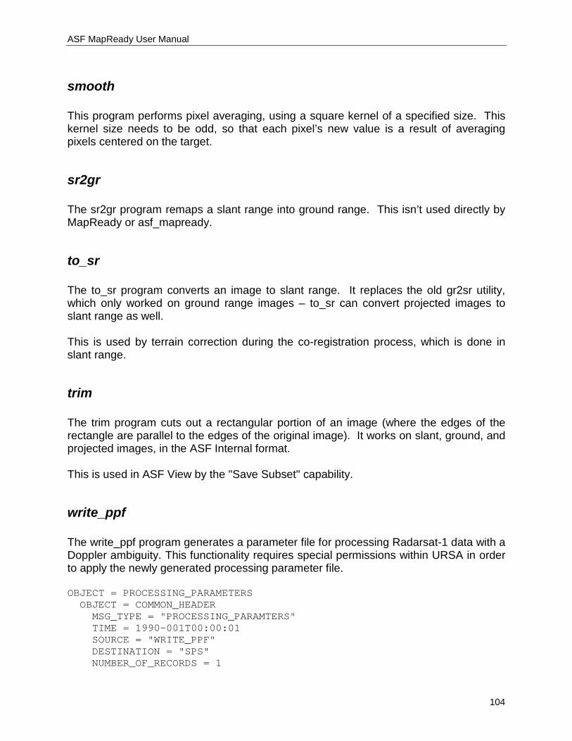
ASF MapReady User Manual
104
smooth This program performs pixel averaging, using a square kernel of a specified size. This kernel size needs to be odd, so that each pixel’s new value is a result of averaging pixels centered on the target.
sr2gr The sr2gr program remaps a slant range into ground range. This isn’t used directly by MapReady or asf_mapready.
to_sr The to_sr program converts an image to slant range. It replaces the old gr2sr utility, which only worked on ground range images – to_sr can convert projected images to slant range as well. This is used by terrain correction during the co-registration process, which is done in slant range.
trim The trim program cuts out a rectangular portion of an image (where the edges of the rectangle are parallel to the edges of the original image). It works on slant, ground, and projected images, in the ASF Internal format. This is used in ASF View by the "Save Subset" capability.
write_ppf The write_ppf program generates a parameter file for processing Radarsat-1 data with a Doppler ambiguity. This functionality requires special permissions within URSA in order to apply the newly generated processing parameter file. OBJECT = PROCESSING_PARAMETERS OBJECT = COMMON_HEADER MSG_TYPE = "PROCESSING_PARAMTERS" TIME = 1990-001T00:00:01 SOURCE = "WRITE_PPF" DESTINATION = "SPS" NUMBER_OF_RECORDS = 1
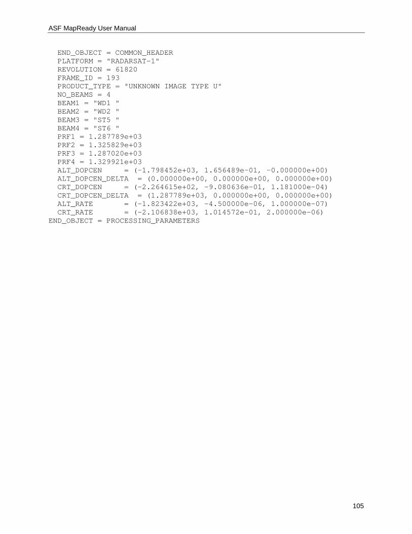
ASF MapReady User Manual
105
END_OBJECT = COMMON_HEADER PLATFORM = "RADARSAT-1" REVOLUTION = 61820 FRAME_ID = 193 PRODUCT_TYPE = "UNKNOWN IMAGE TYPE U" NO_BEAMS = 4 BEAM1 = "WD1 " BEAM2 = "WD2 " BEAM3 = "ST5 " BEAM4 = "ST6 " PRF1 = 1.287789e+03 PRF2 = 1.325829e+03 PRF3 = 1.287020e+03 PRF4 = 1.329921e+03 ALT_DOPCEN = (-1.798452e+03, 1.656489e-01, -0.000000e+00) ALT_DOPCEN_DELTA = (0.000000e+00, 0.000000e+00, 0.000000e+00) CRT_DOPCEN = (-2.264615e+02, -9.080636e-01, 1.181000e-04) CRT_DOPCEN_DELTA = (1.287789e+03, 0.000000e+00, 0.000000e+00) ALT_RATE = (-1.823422e+03, -4.500000e-06, 1.000000e-07) CRT_RATE = (-2.106838e+03, 1.014572e-01, 2.000000e-06) END_OBJECT = PROCESSING_PARAMETERS
ASF MapReady User Manual
106
9. Handling multi-band files with the command line tools The asf_import, asf_geocode and asf_export tools all have a -band option that allows the user to apply their respective functionality to a single band if the passed band identifier can be found in the multi-band image. Command line: asf_import -band 4 ALAV2A037283110-O1B2G_U bahamas Importing: ALAV2A037283110-O1B2G_U Data format: CEOS File: IMG-04-ALAV2A037283110-O1B2G_U Input data type: level two data Output data type: geocoded amplitude image Input band: 04 Processed 8480 of 8480 lines. Import complete. In this example, we are just interested in band 4 of an ALOS AVNIR image and only import this particular band.
ASF MapReady User Manual
107
Appendix A – Configuration File Example This is an example of a complete configuration with full descriptions of each individual parameter. asf_mapready configuration file [General] # This parameter looks for the basename of the input file input file = # This parameter looks for the basename of the ancillary file for # PolSARpro or GAMMA ingest. ancillary file = # This parameter looks for the basename of the output file output file = # Default directory to find files in. If there is no directory in # the input file value, this directory will be appended to it. default input dir = # Default directory to put files in. If there is no directory in # the output file value, this directory will be appended to it. default output dir = # The project flag indicates whether a project needs to be defined. # The project allows the use of naming schemes for output files. # Running asf_mapready with the -create option and the import flag # switched on will generate an [Project] section where you can define further # parameters. project = 0 # The files flag indicates whether a file name list is to be added # to the configuration file. It is strictly used in combination of defining # a project. # Running asf_mapready with the -create option and the import flag # switched on will generate an [Files] section where you can define further # parameters. files = 0 # The import flag indicates whether the data needs to be run through # 'asf_import' (1 for running it, 0 for leaving out the import step). # For example, setting the import switch to zero assumes that all the data # is already in the ASF internal format. # Running asf_mapready with the -create option and the import flag # switched on will generate an [Import] section where you can define further # parameters. import = 1 # If you wish to run an external program on the data after import, # you can set this flag to 1, and then specify the command in
ASF MapReady User Manual
108
# the "[External]" section. external = 0 # The polarimetry flag indicates whether tasks relating to polarimetry will be # performed (1 to enable, 0 to disable). Polarimetric parameters, # decompositions, or classifications can be applied. Faraday rotation correction # can also be applied to the imagery. polarimetry = 1 # The terrain correction flag indicates whether the data needs be run # through 'asf_terrcorr' (1 for running it, 0 for leaving out the terrain # correction step). # Running asf_mapready with the -create option and the terrain correction # flag switched on will generate an [Terrain correction] section where you # can define further parameters. terrain correction = 1 # The calibration flag indicates whether the calibration parameters are # applied to the data through 'asf_calibrate' (1 for running it, 0 for leaving # out the calibration step.) # Running asf_mapready with the -create option and the geocoding flag # switched on will generate a [Calibration] section where you can define further # parameters. calibration = 1 # The geocoding flag indicates whether the data needs to be run through # 'asf_geocode' (1 for running it, 0 for leaving out the geocoding step). # Running asf_mapready with the -create option and the geocoding flag # switched on will generate an [Geocoding] section where you can define further # parameters. geocoding = 1 # The export flag indicates whether the data needs to be run through # 'asf_export' (1 for running it, 0 for leaving out the export step). # Running asf_mapready with the -create option and the export flag # switched on will generate an [Export] section where you can define further # parameters. export = 1 # The mosaic flag indicates whether the data needs to be run through # 'asf_mosaic' (1 for running it, 0 for leaving out the export step). # Running asf_convert with the -create option and the mosaic flag # switched on will generate a [Mosaic] section where you can define further # parameters. mosaic = 0 # The default values file is used to define the user's preferred parameter # settings. In most cases, you will work on a study where your area of interest is # geographically well defined. You want the data for the entire project in the same # projection, with the same pixel spacing and the same output format. # A sample of a default values file can be located in # /home/rudi/tools/fresh/asf_tools/share/asf_tools/mapready/asf_mapready. default values =
ASF MapReady User Manual
109
# The intermediates flag indicates whether the intermediate processing # results are kept (1 for keeping them, 0 for deleting them at the end of the # processing). intermediates = 0 # The short configuration file flag allows the experienced user to # generate configuration files without the verbose comments that explain all # entries for the parameters in the configuration file (1 for a configuration # without comments, 0 for a configuration file with verbose comments) short configuration file = 0 # If you would like to view intermediate imagery, you may wish to turn this # option on -- it dumps an ENVI-compatible .hdr file, that will allow ENVI to view # ASF Internal format .img files. These files are not used by the ASF Tools. dump envi header = 1 # The tmp dir is where temporary files used during processing will # be kept until processing is completed. Then the entire directory and its # contents will be deleted. tmp dir = [Import] # The recognized import formats are: ASF, CEOS, STF, AIRSAR, GEOTIFF # ALOS_MOSAIC, TERRASAR, RADARSAT2, GAMMA or POLSARPRO. # Defining ASF, being the internal format, as the import format is # just another way of actually skipping the import step. For AirSAR, # you can configure which products are processed with the AirSAR block. format = CEOS # The radiometry can be one of the following: AMPLITUDE_IMAGE, # POWER_IMAGE, SIGMA_IMAGE, GAMMA_IMAGE and BETA_IMAGE. # The amplitude image is the regularly processed SAR image. The power image # represents the magnitude (square of the amplitude) of the SAR image. # The sigma, gamma and beta image are different representations of calibrated # SAR images. Their values are in power scale. radiometry = AMPLITUDE_IMAGE # The look up table option is primarily used by the Canadian Ice # Service (CIS) and scales the amplitude values in range direction. The file # parsed in to the import tool is expected to have two columns, the first one # indicating the look angle with the corresponding scale factor as the second # column. look up table = # The latitude constraints (lat begin and lat end) can only be used # when importing level zero swath data (STF). This is the most convenient way # to cut a subset out of a long image swath. lat begin = -99.00 lat end = -99.00 # The precise option, currently under development, will allow the use # of ERS precision state vector from DLR as a replacement of the restituted # state vectors that are provided from the European Space Agency. The parameter
ASF MapReady User Manual
110
# required here defines the location of the precision state vectors. precise = # When the output db flag is non-zero, the calibrated image # is output in decibels. It only applies when the radiometry is sigma, # gamma or beta. output db = 0 # When the complex SLC flag in non-zero, single look complex data is stored in I/Q values. Otherwise SLC data # will be stored as amplitude/phase. complex SLC = 0 # When the multilook SLC flag in non-zero, single look complex data that is stored as amplitude/phase is being # multilooked. multilook SLC = 0 # The ERS2 satellite has a known gain loss problem that this program # will attempt to correct (if this option is turned on) by applying a # scale correction factor uniformly to all pixels in the image. The # correction is dependent on the date, and is only applied to calibrated # data (i.e., everything but amplitude). For more information, see # section 4 of: # <http://www.asf.alaska.edu/reference/dq/Envisat_symp_ers2_performance.pdf> apply ers2 gain fix = 1 # If any input files are PolSARpro files, then it will be a single-band # greyscale image containing a PolSARpro classification. In order for the classification # to be properly colored, a PolSARpro look-up table should be specified here. # For a full list of available PolSARpro look-up tables, look in the ASF Tools # share directory. The available look-up tables can be found in the following # path: <path>/asf_tools/share/asf_tools/mapready/look_up_tables. In this folder, # you will find files ending in ".lut" and ".pal". Only the .pal files can # be applied to PolSARpro files ...They originated from PolSARpro and are named # according to the PolSARpro classification to which they apply. NOTE: This field # is OPTIONAL and only applies if you are processing PolSARpro files. If not, # then you may leave this field blank. If it is blank, then any PolSARpro data # that is processed will remain (non-meaningfully) greyscale. polsarpro colormap = # The image data type is only relevant for PolSARPro ingest. # It determines whether the input needs to be as a matrix or a file. # Current options: POLARIMETRIC_SEGMENTATION, POLARIMETRIC_DECOMPOSITION, # POLARIMETRIC_PARAMETERS and POLARIMETRIC_MATRIX, image data type = # If the name of the metadata file is not deducible from the name # given for the input file, it can be specified here. Currently, only GAMMA # data needs to do this, for other types of data either the input file is # the metadata, or the metadata filename follows a standard naming convention. # If you have renamed your metadata file against the standard naming scheme # for the data, you should rename it back rather than using this option. metadata file =
ASF MapReady User Manual
111
# The interferometric GAMMA data consists of several data sets. # The interferogram is stored as complex floating point values. interferogram = # The interferometric GAMMA data consists of several data sets. # The coherence image is stored in floating point values between 0 and 1. coherence = # The interferometric GAMMA data consists of several data sets. # The metadata of the SLC slave image is used to define the temporal # baseline. slave metadata = # The interferometric GAMMA data consists of several data sets. # This file contains the baseline components that describe the geometry of # the interferometric pairs. baseline = # The interferometric GAMMA data can be stored in complex form. # This flag is providing generic support for any complex GAMMA file, # regardless what nature the data is. complex gamma = 0 # The UAVSAR ingest requires the definition of which product actually needs # to be imported. # PolSAR products: SLC,MLC,DAT,GRD,HGT # InSAR products: AMP,INT,UNW,COR,AMP_GRD,INT_GRD,UNW_GRD,COR_GRD,HGT_GRD # Several products can be ingested at the same by listed them comma separated. # By setting this parameter to 'all', all available products are imported. uavsar = [Polarimetry] # If you have quad-pol SLC data available, # you can use the standard Pauli decomposition to map the 4 bands to # the R, G, and B channels in the output image. In this decomposition, # red is HH-VV, green is HV, and blue is HH+VV. In addition, each channel # will individually contrast-expanded using a 2-sigma remapping for improved # visualization. pauli = 0 # If you have quad-pol data available (HH, HV, VH and VV), # you can use the standard Sinclair decomposition to map the 4 bands to # the R, G, and B channels in the output image. In this decomposition, # red is VV, green is (HV+VH)/2, and blue is HH. In addition, each channel # will individually contrast-expanded using a 2-sigma remapping for improved # visualization. sinclair = 0 # If you have quad_pol SLC data available), # you can use the Cloude-Pottier classification using entropy and alpha # to map the 4 bands to the eight classes in one band in the output image.

ASF MapReady User Manual
112
cloude pottier = 0 # If you have quad_pol SLC data available), # you can use the extended Cloude-Pottier classification using entropy, alpha # and anisotropy to map the 4 bands to the 16 classes in one band in the output image. extended cloude pottier = 0 # If you have quad_pol SLC data available, # you can have the entropy, anisotropy, and alpha values (the values used # in the Cloude Pottier classification) output in three separate # bands. This can be useful if you plan on doing your own classification, # or simply wish to inspect the raw entropy, anisotropy, and/or alpha data. entropy anisotropy alpha = 0 # If you have quad-pol SLC data available, # you can use the Freeman/Durden decomposition to map the 4 bands to # the R, G, and B channels in the output image. In this decomposition, # the red channel represents the amount of double-bounce contribution, # the green channel represents the rough-surface contribution, and # the blue channel represents the volume scatterer contribution. freeman durden = 0 # Quad-pol SLC data (HH, HV, VH and VV bands in both phase & amplitude) # must be available in order to use Faraday rotation correction. This # functionality corrects for atmospheric conditions that rotate the # polarity of the SAR beam. A 0 value indicates that the correction is # turned off. A value of 1 uses a single rotation angle for the entire # image; the single angle is the average of all the per-pixel angles. # A value of 2 uses a local average of the per pixel angles. faraday correction = 0 # If the Faraday Rotation angle is small, you can elect to # not apply the correction, even if you have selected to above. # If the correction angle is smaller than the threshold angle, then # the correction is not applied. Use -1 for no threshold (which means # the correction is always applied). farcorr threshold = -1.00 [Terrain correction] # This parameter defines the output size of the terrain corrected # image. If set to -99 this parameter will be ignored and the 'asf_terrcorr' will # deal with the issues that might occur when using different pixel spacings in # the SAR image and the reference DEM pixel spacing = -99.00 # The heights of the reference DEM are used to correct the SAR image # for terrain effects. The quality and resolution of the reference DEM determines # the quality of the resulting terrain corrected product digital elevation model = # In some case parts of the images are known to be moving (e.g. water,

ASF MapReady User Manual
113
# glaciers etc.). This can cause severe problems in matching the SAR image with # the simulated SAR image derived from the reference. Providing a mask defines the # areas that are stable and can be used for the matching process. mask = # Instead of creating a mask, you can have terrain correction # automatically generate a mask for you, based on the DEM, which attempts to mask # the regions of your scene that are water (these regions provide a poor match). # Specifically, all DEM values <1m are masked, unless a different height cutoff # is specified with the 'water height cutoff' option, described next. auto mask water = 0 # When creating a mask automatically with the previous flag, # you may specify use a value other than 1m as the height cutoff. # This value is ignored when 'auto mask water' is 0. water height cutoff = 1.000000 # When applying a mask during terrain correction, you can choose # how the regions covered by the mask are filled in the final terrain corrected # result. You can either specify a (non-negative) value of your choosing,or # if you'd like the SAR data to be kept then use -1 as the fill value. fill value = 0 # Normally during terrain correction, only geometric terrain is # applied. This option will also turn on radiometric terrain correction. # This option is still experimental. The correction adjusts the values to # account for the actual incidence angle (using the DEM), instead of the # estimated incidence angle (using the Earth-as-ellipsoid) used during # processing. do radiometric = 0 # If your DEM has a number of "holes" in it, this can cause streaking # in the terrain corrected product. This option will attempt to replace DEM holes # with interpolated values. smooth dem holes = 0 # If the DEM has a pixel size that is significantly larger (a factor # of 2) than the SAR image, by default the SAR image is downsampled # to a pixel size half that of the DEM. With this option set to 1, no # resampling of this type will be done. However, the quality of the # terrain corrected product is still limited by the resolution of # the DEM. By default, this option is off (0). no resampling = 0 # Even if you don't want to change the image via terrain correction, # you may still wish to use the DEM to refine the geolocation of the SAR image. # If this flag is set, terrain correction is NOT performed. refine geolocation only = 0 # Layover/shadow regions can either be left black (resulting in better # image statistics in the remainder of the image), or they may be interpolated over # (resulting in a nicer-looking image). Setting this parameter to 1 indicates that # these regions should be interpolated over. interpolate = 1
ASF MapReady User Manual
114
# The DEM that is provided is clipped to match the scene. Normally this # clipped DEM is removed along with the other temporary files, however if you are # interested you can turn this option on (set it to 1), which will keep the clipped # DEM, as well as geocode (if you've elected to geocode) and export it (if you've # elected to export, though the DEM is always exported as floating point data even # when you exporting your SAR data as bytes). The clipped DEM will be slightly # larger than the SAR image, usually, since a larger region must be clipped to # allow for the height variations. save terrcorr dem = 0 # This option determines if a file marking the regions of layover and # shadow should be created along with the output image. It is geocoded using the # the same parameters as your SAR image, and exported as byte data. save terrcorr layover mask = 0 # This option determines if the simulated image derived from the DEM is # used for matching with the SAR image in slant range. If you don't trust the quality # of the orbital information or want to determine your own offset, you want to switch # this flag to 1. no matching = 0 # This parameter sets the offset in range direction in case the simulated # amplitude derived from the DEM is NOT used for matching with the slant range SAR # image. The offset is specified in meters. range offset = 0.000000 # This parameter sets the offset in azimuth direction in case the simulated # amplitude derived from the DEM is NOT used for matching with the slant range SAR # image. The offset is specified in meters. azimuth offset = 0.000000 # The DEM that is provided to asf_terrcorr is generally in ground range, # and is converted to slant range as part of the coregistration procedure. # After coregistration, you can use either the original ground range DEM, or # the slant range DEM, to do the actual terrain correction. By default, the # slant range DEM is used, specifying 'use gr dem = 1' will use the ground range # DEM. The choice only makes a significant difference in regions of layover; # both produce similar results in areas without layover. Using the slant range # DEM results in more aggressive interpolations, which sometimes results in # streaky-looking layover regions, whereas using the ground range DEM preserves # more structure within the layover regions, but can look worse if the # coregistration is off in those areas. use gr dem = 0 # This option causes terrain correction to try to use the DEM # to refine the geolocation of the SAR image before terrain correcting, # but if this fails then proceed with terrain correction anyway, using # offsets of zero. (I.e., assume the geolocation of the SAR image is # good enough for terrain correction.) This often produces good # results, especially if the terrain is fairly flat. When this option # if turned off (i.e., set to zero, the default), terrain correction # will abort with an error if the coregistration fails. use zero offsets if match fails = 0 # Turning this on saves an intermediate product with the
ASF MapReady User Manual
115
# incidence angles and correction factors determined during radiometric # terrain correction. Use this option only when radiometric # correction is turned on save incidence angles = 0 [Calibration] # The radiometry can be one of the following: AMPLITUDE_IMAGE, # POWER_IMAGE, SIGMA_IMAGE, GAMMA_IMAGE and BETA_IMAGE. # The amplitude image is the regularly processed SAR image. The power image # represents the magnitude (square of the amplitude) of the SAR image. # The sigma, gamma and beta image are different representations of calibrated # SAR images. Their values are in power scale. radiometry = AMPLITUDE_IMAGE # This parameter indicates whether the data is scaled back # to byte using a formula developed by Woods Hole. woods hole scale = 0 [Geocoding] # The geocoding tool currently supports five different map projections: # Universal Transverse Mercator (UTM), Polar Stereographic, Albers Equal Area # Conic, Lambert Conformal Conic and Lambert Azimuthal Equal Area. # For all these map projections a large number of projection parameter files # have been predefined for various parts of the world. # The projection parameter files are located in: # /home/rudi/tools/fresh/asf_tools/share/asf_tools/mapready/projections projection = /home/rudi/tools/fresh/asf_tools/share/asf_tools/mapready/projections/utm/utm.proj # The pixel spacing determines the pixel size used for the resulting # geocoded image and, therefore, the size of the output image. pixel spacing = -99.00 # An average height can be defined for the image that is taken into # account and adjusted for during the geocoding process. height = 0.0 # Three different resampling methods have been implemented as part # of the geocoding: NEAREST NEIGHBOR, BILINEAR and BICUBIC. The bilinear # resampling method is the default. resampling = BILINEAR # After geocoding, a fill value is required for the regions outside # of the geocoded image. By default this value is 0, but may be set to a # different value here. background = 0.00 # In order to ensure the proper use of projection parameter files, # we have implemented a number of checks that verify whether the map # projection parameters are reasonable for the area that is covered by the # data. For example, applying a projection parameter file that is defined for
ASF MapReady User Manual
116
# South America for a data set that is covering Alaska would lead to huge # distortions. These checks can be overwritten by setting the force option. force = 0 [Export] # The following format are considered valid format: ASF, TIFF, GEOTIFF # JPEG, PNG, PGM and POLSARPRO. # In the same way as for the import block, ASF as an export option results in # skipping the export step entirely. All other formats, with the exception of # GeoTIFF, require the scaling of the internal ASF format from floating point # to byte. The GeoTIFF supports byte as well as floating point data. format = GEOTIFF # The byte conversion options are SIGMA, MINMAX, TRUNCATE or # HISTOGRAM_EQUALIZE. They scale the floating point values to byte values. byte conversion = SIGMA # Applies a look-up-table to the greyscale values, to convert them to RGB, # using the table in with the given filename. Only allowed for single-band # images. Some look up table files are in the look_up_tables subdirectory # in the ASF tools share directory. The tool will look in the share # directory, if the given look up table file is not found. rgb look up table = # If you have more than one band available in your data, you can # create the exported file using the different bands for the R, G, and B # channels in the output image. List the R, G, and B channels in that order # separated by commas. E.g. HH,HV,VV. Note that no contrast expansion or # other modification of the data will be applied. rgb banding = # If you have 3+ bands available in your optical data, # you can create the exported file using a standard selection of bands for # the R, G, and B channels in the output image. By setting the truecolor # flag, band assignments will be R = 3, G = 2, and B = 1 and each band # will individually contrast-expanded using a 2-sigma remapping for improved # visualization (use rgb banding if you desire raw data assignments.) truecolor = 0 # If you have 4 bands available in your optical data, # you can create the exported file using a standard selection of bands for # the R, G, and B channels in the output image. By setting the falsecolor # flag, band assignments will be R = 4, G = 3, and B = 2 and each band # will individually contrast-expanded using a 2-sigma remapping for improved # visualization (use rgb banding if you desire raw data assignments.) falsecolor = 0 # If you wish to export a single band from the list of # available bands, e.g. HH, HV, VH, VV ...enter VV to export just # the VV band (alone.) band =
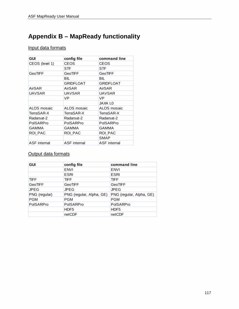
ASF MapReady User Manual
117
Appendix B – MapReady functionality
Input data formats
GUI config file command lineCEOS (level 1) CEOS CEOS
STF STFGeoTIFF GeoTIFF GeoTIFF
BIL BILGRIDFLOAT GRIDFLOAT
AirSAR AirSAR AirSARUAVSAR UAVSAR UAVSAR
VP VPJAXA L0
ALOS mosaic ALOS mosaic ALOS mosaicTerraSAR-X TerraSAR-X TerraSAR-XRadarsat-2 Radarsat-2 Radarsat-2PolSARPro PolSARPro PolSARProGAMMA GAMMA GAMMAROI_PAC ROI_PAC ROI_PAC
SMAPASF internal ASF internal ASF internal
Output data formats
GUI config file command lineENVI ENVIESRI ESRI
TIFF TIFF TIFFGeoTIFF GeoTIFF GeoTIFFJPEG JPEG JPEGPNG (regular) PNG (regular, Alpha, GE) PNG (regular, Alpha, GE)PGM PGM PGMPolSARPro PolSARPro PolSARPro
HDF5 HDF5netCDF netCDF
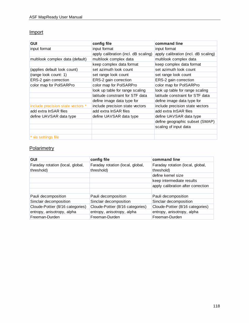
ASF MapReady User Manual
118
Import
GUI config file command lineinput format input format input format
apply calibration (incl. dB scaling) apply calibration (incl. dB scaling)multilook complex data (default) multilook complex data multilook complex data
keep complex data format keep complex data format(applies default look count) set azimuth look count set azimuth look count(range look count: 1) set range look count set range look countERS-2 gain correction ERS-2 gain correction ERS-2 gain correctioncolor map for PolSARPro color map for PolSARPro color map for PolSARPro
look up table for range scaling look up table for range scalinglatitude constraint for STF data latitude constraint for STF datadefine image data type for define image data type for
include precision state vectors * include precision state vectors include precision state vectorsadd extra InSAR files add extra InSAR files add extra InSAR filesdefine UAVSAR data type define UAVSAR data type define UAVSAR data type
define geographic subset (SMAP)scaling of input data
* via settings file
Polarimetry
GUI config file command lineFaraday rotation (local, global, threshold)
Faraday rotation (local, global, threshold)
Faraday rotation (local, global, threshold)define kernel sizekeep intermediate resultsapply calibration after correction
Pauli decomposition Pauli decomposition Pauli decompositionSinclair decomposition Sinclair decomposition Sinclair decompositionCloude-Pottier (8/16 categories) Cloude-Pottier (8/16 categories) Cloude-Pottier (8/16 categories)entropy, anisotropy, alpha entropy, anisotropy, alpha entropy, anisotropy, alphaFreeman-Durden Freeman-Durden Freeman-Durden
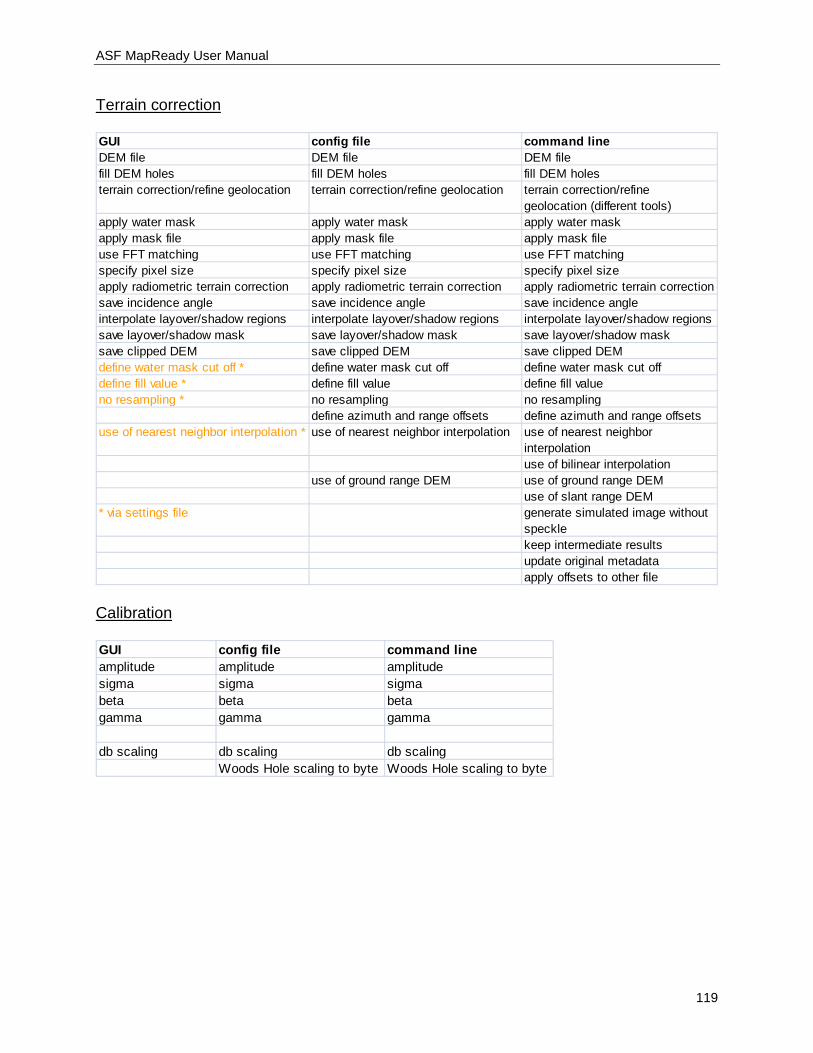
ASF MapReady User Manual
119
Terrain correction
GUI config file command lineDEM file DEM file DEM filefill DEM holes fill DEM holes fill DEM holesterrain correction/refine geolocation terrain correction/refine geolocation terrain correction/refine
geolocation (different tools)apply water mask apply water mask apply water maskapply mask file apply mask file apply mask fileuse FFT matching use FFT matching use FFT matchingspecify pixel size specify pixel size specify pixel sizeapply radiometric terrain correction apply radiometric terrain correction apply radiometric terrain correctionsave incidence angle save incidence angle save incidence angleinterpolate layover/shadow regions interpolate layover/shadow regions interpolate layover/shadow regionssave layover/shadow mask save layover/shadow mask save layover/shadow masksave clipped DEM save clipped DEM save clipped DEMdefine water mask cut off * define water mask cut off define water mask cut offdefine fill value * define fill value define fill valueno resampling * no resampling no resampling
define azimuth and range offsets define azimuth and range offsetsuse of nearest neighbor interpolation * use of nearest neighbor interpolation use of nearest neighbor
interpolationuse of bilinear interpolation
use of ground range DEM use of ground range DEMuse of slant range DEM
* via settings file generate simulated image without specklekeep intermediate resultsupdate original metadataapply offsets to other file
Calibration
GUI config file command lineamplitude amplitude amplitudesigma sigma sigmabeta beta betagamma gamma gamma
db scaling db scaling db scalingWoods Hole scaling to byte Woods Hole scaling to byte
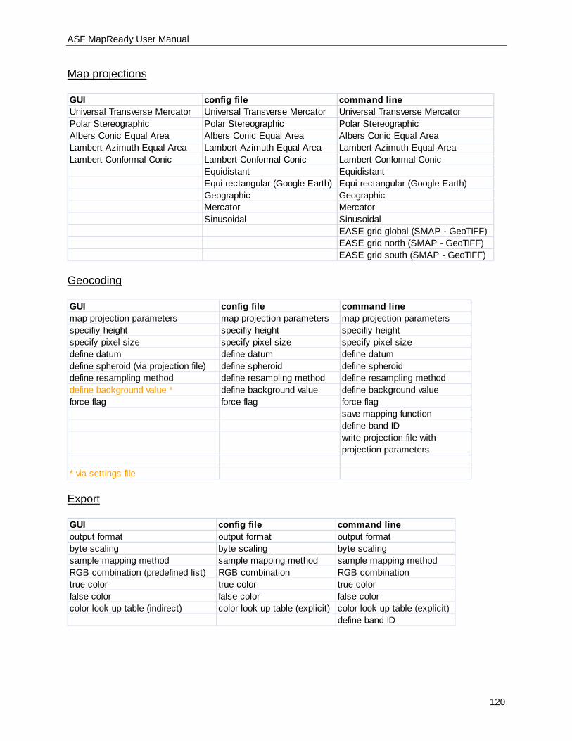
ASF MapReady User Manual
120
Map projections
GUI config file command lineUniversal Transverse Mercator Universal Transverse Mercator Universal Transverse MercatorPolar Stereographic Polar Stereographic Polar StereographicAlbers Conic Equal Area Albers Conic Equal Area Albers Conic Equal AreaLambert Azimuth Equal Area Lambert Azimuth Equal Area Lambert Azimuth Equal AreaLambert Conformal Conic Lambert Conformal Conic Lambert Conformal Conic
Equidistant EquidistantEqui-rectangular (Google Earth) Equi-rectangular (Google Earth)Geographic GeographicMercator MercatorSinusoidal Sinusoidal
EASE grid global (SMAP - GeoTIFF)EASE grid north (SMAP - GeoTIFF)EASE grid south (SMAP - GeoTIFF)
Geocoding
GUI config file command linemap projection parameters map projection parameters map projection parametersspecifiy height specifiy height specifiy heightspecify pixel size specify pixel size specify pixel sizedefine datum define datum define datumdefine spheroid (via projection file) define spheroid define spheroiddefine resampling method define resampling method define resampling methoddefine background value * define background value define background valueforce flag force flag force flag
save mapping functiondefine band IDwrite projection file with projection parameters
* via settings file
Export
GUI config file command lineoutput format output format output formatbyte scaling byte scaling byte scalingsample mapping method sample mapping method sample mapping methodRGB combination (predefined list) RGB combination RGB combinationtrue color true color true colorfalse color false color false colorcolor look up table (indirect) color look up table (explicit) color look up table (explicit)
define band ID