artificial neural networks for rf and microwave design-from theory to

IEEE TRANSACTIONS ON MICROWAVE THEORY AND TECHNIQUES, VOL. 51, NO. 4, APRIL 2003 1339

Artificial Neural Networks for RF and MicrowaveDesign—From Theory to Practice

Qi-Jun Zhang, Senior Member, IEEE, Kuldip C. Gupta, Fellow, IEEE, andVijay K. Devabhaktuni, Student Member, IEEE

Abstract—Neural-network computational modules have re-cently gained recognition as an unconventional and useful tool forRF and microwave modeling and design. Neural networks can betrained to learn the behavior of passive/active components/circuits.A trained neural network can be used for high-level design, pro-viding fast and accurate answers to the task it has learned. Neuralnetworks are attractive alternatives to conventional methods suchas numerical modeling methods, which could be computationallyexpensive, or analytical methods which could be difficult to obtainfor new devices, or empirical modeling solutions whose range andaccuracy may be limited. This tutorial describes fundamentalconcepts in this emerging area aimed at teaching RF/microwaveengineers what neural networks are, why they are useful, whenthey can be used, and how to use them. Neural-network structuresand their training methods are described from the RF/microwavedesigner’s perspective. Electromagnetics-based training forpassive component models and physics-based training for activedevice models are illustrated. Circuit design and yield optimiza-tion using passive/active neural models are also presented. Amultimedia slide presentation along with narrative audio clips isincluded in the electronic version of this paper. A hyperlink tothe NeuroModeler demonstration software is provided to allowreaders practice neural-network-based design concepts.

Index Terms—Computer-aided design (CAD), designautomation, modeling, neural networks, optimization, simulation.

I. INTRODUCTION

NEURAL networks, also called artificial neural networks(ANNs), are information processing systems with their

design inspired by the studies of the ability of the human brainto learn from observations and to generalize by abstraction [1].The fact that neural networks can be trained to learn any arbi-trary nonlinear input–output relationships from correspondingdata has resulted in their use in a number of areas such aspattern recognition, speech processing, control, biomedicalengineering etc. Recently, ANNs have been applied to RF andmicrowave computer-aided design (CAD) problems as well.

Manuscript received April 25, 2002.Q.-J. Zhang and V. K. Devabhaktuni are with the Department of

Electronics, Carleton University, Ottawa, ON, Canada K1S 5B6 (e-mail:[email protected]; [email protected]).

K. C. Gupta is with the Department of Electrical and ComputerEngineering, University of Colorado at Boulder, Boulder, CO 80309 USAand also with Concept-Modules LLC, Boulder, CO 80303 USA (e-mail:[email protected]).

This paper has supplementary downloadable material available at http://iee-explore.ieee.org, provided by the authors. This includes a Microsoft PowerPointslide presentation including narrative audio clips and animated transitions. A hy-perlink to a Web demonstration of theNeuroModelerprogram is provided in thelast slide. This material is 31.7 MB in size.

Digital Object Identifier 10.1109/TMTT.2003.809179

Neural networks are first trained to model the electrical be-havior of passive and active components/circuits. These trainedneural networks, often referred to as neural-network models(or simply neural models), can then be used in high-levelsimulation and design, providing fast answers to the task theyhave learned [2], [3]. Neural networks are efficient alternativesto conventional methods such as numerical modeling methods,which could be computationally expensive, or analyticalmethods, which could be difficult to obtain for new devices,or empirical models, whose range and accuracy could belimited. Neural-network techniques have been used for a widevariety of microwave applications such as embedded passives[4], transmission-line components [5]–[7], vias [8], bends [9],coplanar waveguide (CPW) components [10], spiral inductors[11], FETs [12], amplifiers [13], [14], etc. Neural networkshave also been used in impedance matching [15], inversemodeling [16], measurements [17], and synthesis [18].

An increased number of RF/microwave engineers andresearchers have started taking serious interest in this emergingtechnology. As such, this tutorial is prepared to meet the edu-cational needs of the RF/microwave community. The subjectof neural networks will be described from the point-of-view ofRF/microwave engineers using microwave-oriented languageand terminology. In Section II, neural-network structural issuesare introduced, and the popularly used multilayer percep-tron (MLP) neural network is described at length. Varioussteps involved in the development of neural-network modelsare described in Section III. Practical microwave examplesillustrating the application of neural-network techniques tocomponent modeling and circuit optimization are presented inSections IV and V, respectively. Finally, Section VI containsa summary and conclusions. To further aid the readers inquickly grasping the ANN fundamentals and practical aspects,an electronic multimedia slide presentation of the tutorial anda hyperlink to NeuroModelerdemonstration software1 areincluded in the CD-ROM accompanying this issue.

II. NEURAL-NETWORK STRUCTURES

We describe neural-network structural issues to betterunderstand what neural networks are and why they have theability to represent RF and microwave component behaviors.We study neural networks from the external input–outputpoint-of-view, and also from the internal neuron information

1NeuroModeler, Q.-J. Zhang, Dept. Electron., Carleton Univ., Ottawa, ON,Canada.

0018-9480/03$17.00 © 2003 IEEE

1340 IEEE TRANSACTIONS ON MICROWAVE THEORY AND TECHNIQUES, VOL. 51, NO. 4, APRIL 2003

Fig. 1. Physics-based FET to be modeled using a neural network.

processing point-of-view. The most popularly used neural-net-work structure, i.e., the MLP, is described in detail. The effectsof structural issues on modeling accuracy are discussed.

A. Basic Components

A typical neural-network structure has two types of basiccomponents, namely, the processing elements and the intercon-nections between them. The processing elements are called neu-rons and the connections between the neurons are known aslinks or synapses. Every link has a corresponding weight param-eter associated with it. Each neuron receives stimulus from otherneurons connected to it, processes the information, and pro-duces an output. Neurons that receive stimuli from outside thenetwork are called input neurons, while neurons whose outputsare externally used are called output neurons. Neurons that re-ceive stimuli from other neurons and whose outputs are stimulifor other neurons in the network are known as hidden neurons.Different neural-network structures can be constructed by usingdifferent types of neurons and by connecting them differently.

B. Concept of a Neural-Network Model

Let and represent the number of input and output neuronsof a neural network. Let be an -vector containing the externalinputs to the neural network, be an -vector containing theoutputs from the output neurons, andbe a vector containingall the weight parameters representing various interconnectionsin the neural network. The definition of, and the manner inwhich is computed from and , determine the structure ofthe neural network.

Consider an FET as shown in Fig. 1. The physical/geomet-rical/bias parameters of the FET are variables and any changein the values of these parameters affects the electrical responsesof the FET (e.g., small-signal -parameters). Assume thatthere is a need to develop a neural model that can representsuch input–output relationship. Inputs and outputs of thecorresponding FET neural model are given by

(1)

(2)

where is frequency, and and represent magni-tude and phase of the-parameter . The superscript in-dicates transpose of a vector or matrix. Other parameters in (1)

are defined in Fig. 1. The original physics-based FET modelingproblem can be expressed as

(3)

where is a detailed physics-based input–output relationship.The neural-network model for the FET is given by

(4)

The neural network in (4) can represent the FET behavior in(3) only after learning the original– relationship through aprocess called training. Several (, ) samples called trainingdata need to be generated either from the FET’s physicssimulator or from measurements. The objective of training isto adjust neural-network weights such that the neural modeloutputs best match the training data outputs. A trained neuralmodel can be used during the microwave design process toprovide instant answers to the task it has learned. In the FETcase, the neural model can be used to provide fast estimationof -parameters against the FET’s physical/geometrical/biasparameter values.

C. Neural Network Versus Conventional Modeling

The neural-network approach can be compared with conven-tional approaches for a better understanding. The first approachis the detailed modeling approach (e.g., electromagnetic(EM)-based models for passive components and physics-basedmodels for active devices), where the model is defined by awell-established theory. The detailed models are accurate, butcould be computationally expensive. The second approach is anapproximate modeling approach, which uses either empiricalor equivalent-circuit-based models for passive and activecomponents. These models are developed using a mixtureof simplified component theory, heuristic interpretation andrepresentation, and/or fitting of experimental data. Evaluationof approximate models is much faster than that of the detailedmodels. However, the models are limited in terms of accuracyand input parameter range over which they can be accurate.The neural-network approach is a new type of modelingapproach where the model can be developed by learning fromdetailed (accurate) data of the RF/microwave component. Aftertraining, the neural network becomes a fast and accurate modelrepresenting the original component behaviors.

D. MLP Neural Network

1) Structure and Notation:MLP is a popularly used neural-network structure. In the MLP neural network, the neurons aregrouped into layers. The first and the last layers are called inputand output layers, respectively, and the remaining layers arecalled hidden layers. Typically, an MLP neural network consistsof an input layer, one or more hidden layers, and an output layer,as shown in Fig. 2. For example, an MLP neural network withan input layer, one hidden layer, and an output layer, is referredto as three-layer MLP (or MLP3).

Suppose the total number of layers is. The first layer is theinput layer, the th layer is the output layer, and layers 2 toare hidden layers. Let the number of neurons in theth layer be

, . Let represent the weight of the link

ZHANG et al.: ANNs FOR RF AND MICROWAVE DESIGN 1341

Fig. 2. MLP neural-network structure. Typically, an MLP network consists ofan input layer, one or more hidden layers, and an output layer.

between theth neuron of the th layer and theth neuron ofthe th layer. Let represent theth external input to the MLPand be the output of theth neuron of theth layer. There is anadditional weight parameter for each neuron () representingthe bias for the th neuron of theth layer. As such, of theMLP includes , , , and

, i.e., .The parameters in the weight vector are real numbers, whichare initialized before MLP training. During training, they arechanged (updated) iteratively in a systematic manner [19]. Oncethe neural-network training is completed, the vectorremainsfixed throughout the usage of the neural network as a model.

2) Anatomy of Neurons:In the MLP network, each neuronprocesses the stimuli (inputs) received from other neurons. Theprocess is done through a function called the activation func-tion in the neuron, and the processed information becomes theoutput of the neuron. For example, every neuron in theth layerreceives stimuli from the neurons of the ( )th layer, i.e., ,

, , . A typical th neuron in theth layer processesthis information in two steps. Firstly, each of the inputs is mul-tiplied by the corresponding weight parameter and the productsare added to produce a weighted sum, i.e.,

(5)

In order to create the effect of bias parameter, we assume afictitious neuron in the ( )th layer whose output is. Secondly, the weighted sum in (5) is used to activate the

neuron’s activation function to produce the final output ofthe neuron . This output can, in turn, become the

stimulus to neurons in the ( )th layer. The most commonlyused hidden neuron activation function is the sigmoid functiongiven by

(6)

Other functions that can also be used are the arc-tangentfunction, hyperbolic-tangent function, etc. All these are smoothswitch functions that are bounded, continuous, monotonic, andcontinuously differentiable. Input neurons use a relay activationfunction and simply relay the external stimuli to the hiddenlayer neurons, i.e., , . In the case ofneural networks for RF/microwave design, where the purposeis to model continuous electrical parameters, a linear activationfunction can be used for output neurons. An output neuroncomputation is given by

(7)

3) Feedforward Computation:Given the input vectorand the weight vector , neural network

feedforward computation is a process used to compute theoutput vector . Feedforward computationis useful not only during neural-network training, but alsoduring the usage of the trained neural model. The externalinputs are first fed to the input neurons (i.e., first layer) and theoutputs from the input neurons are fed to the hidden neuronsof the second layer. Continuing this way, the outputs of the

th layer neurons are fed to the output layer neurons (i.e.,the th layer). During feedforward computation, neural-net-work weights remain fixed. The computation is given by

(8)

(9)

(10)

4) Important Features:It may be noted that the simpleformulas in (8)–(10) are now intended for use as RF/microwavecomponent models. It is evident that these formulas are mucheasier to compute than numerically solving theoretical EMor physics equations. This is the reason why neural-networkmodels are much faster than detailed numerical models ofRF/microwave components. For the FET modeling exampledescribed earlier, (8)–(10) will represent the model of-pa-rameters as functions of transistor gate length, gate width,doping density, and gate and drain voltages. The question ofwhy such simple formulas in the neural network can representcomplicated FET (or, in general, EM, physics, RF/microwave)behavior can be answered by the universal approximationtheorem.

The universal approximation theorem [20] states that therealways exists a three-layer MLP neural network that can ap-proximate any arbitrary nonlinear continuous multidimensionalfunction to any desired accuracy. This forms a theoretical basis


for employing neural networks to approximate RF/microwavebehaviors, which can be functions of physical/geometrical/biasparameters. MLP neural networks are distributed models, i.e.,no single neuron can produce the overall– relationship.For a given , some neurons are switched on, some are off,and others are in transition. It is this combination of neuronswitching states that enables the MLP to represent a givennonlinear input–output mapping. During training process,the MLP’s weight parameters are adjusted and, at the end oftraining, they encode the component information from thecorresponding – training data.

E. Network Size and Layers

For the neural network to be an accurate model of the problemto be learned, a suitable number of hidden neurons are needed.The number of hidden neurons depends upon the degree of non-linearity of and the dimensionality of and (i.e., values ofand ). Highly nonlinear components need more neurons andsmoother items need fewer neurons. However, the universal ap-proximation theorem does not specify as to what should be thesize of the MLP network. The precise number of hidden neuronsrequired for a given modeling task remains an open question.Users can use either experience or a trial-and-error process tojudge the number of hidden neurons. The appropriate numberof neurons can also be determined through adaptive processes,which add/delete neurons during training [4], [21]. The numberof layers in the MLP can reflect the degree of hierarchical infor-mation in the original modeling problem. In general, the MLPswith one or two hidden layers [22] (i.e., three- or four-layerMLPs) are commonly used for RF/microwave applications.

F. Other Neural-Network Configurations

In addition to the MLP, there are other ANN structures [19],e.g., radial basis function (RBF) networks, wavelet networks,recurrent networks, etc. In order to select a neural-networkstructure for a given application, one starts by identifying thenature of the – relationship. Nondynamic modeling problems(or problems converted from dynamic to nondynamic usingmethods like harmonic balance) can be solved using MLP, RBF,and wavelet networks. The most popular choice is the MLPsince its structure and training are well-established. RBF andwavelet networks can be used when the problem exhibits highlynonlinear and localized phenomena (e.g., sharp variations).Time-domain dynamic responses such as those in nonlinearmodeling can be represented using recurrent neural networks[13] and dynamic neural networks [14]. One of the most recentresearch directions in the area of microwave-oriented ANNstructures is the knowledge-based networks [6]–[9], whichcombine existing engineering knowledge (e.g., empiricalequations and equivalent-circuit models) with neural networks.

III. N EURAL-NETWORK MODEL DEVELOPMENT

The neural network does not represent any RF/microwavecomponent unless we train it with RF/microwave data. Todevelop a neural-network model, we need to identify inputand output parameters of the component in order to generateand preprocess data, and then use this data to carry out ANN

training. We also need to establish quality measures of neuralmodels. In this section, we describe the important steps andissues in neural model development.

A. Problem Formulation and Data Processing

1) ANN Inputs and Outputs:The first step toward devel-oping a neural model is the identification of inputs andoutputs . The output parameters are determined based on thepurpose of the neural-network model. For example, real andimaginary parts of -parameters can be selected for passivecomponent models, currents and charges can be used forlarge-signal device models, and cross-sectional resistance–in-ductance–conductance–capacitance (RLGC) parameters canbe chosen for very large scale integration (VLSI) interconnectmodels. Other factors influencing the choice of outputs are:1) ease of data generation; 2) ease of incorporation of the neuralmodel into circuit simulators, etc. Neural model input param-eters are those device/circuit parameters (e.g., geometrical,physical, bias, frequency, etc.) that affect the output parametervalues.

2) Data Range and Sample Distribution:The next step is todefine the range of data to be used in ANN model developmentand the distribution of – samples within that range. Supposethe range of input space (i.e.,-space) in which the neural modelwould be used after training (during design) is , .Training data is sampled slightly beyond the model utilizationrange, i.e., , , in order to ensure reliabilityof the neural model at the boundaries of model utilization range.Test data is generated in the range , .

Once the range of input parameters is finalized, a samplingdistribution needs to be chosen. Commonly used sample dis-tributions include uniform grid distribution, nonuniform griddistribution, design of experiments (DOE) methodology [8], stardistribution [9], and random distribution. In uniform grid dis-tribution, each input parameter is sampled at equal intervals.Suppose the number of grids along input dimensionis . Thetotal number of – samples is given by . For ex-ample, in an FET modeling problem whereand neural model utilization range is

(11)

training data can be generated in the range

(12)

In nonuniform grid distribution, each input parameter is sam-pled at unequal intervals. This is useful when the problem be-havior is highly nonlinear in certain subregions of the-spaceand dense sampling is needed in such subregions. Modelingdc characteristics (– curves) of an FET is a classic examplefor nonuniform grid distribution. Sample distributions based onDOE (e.g., factorial experimental design, central compositeexperimental design) and star distribution are used in situationswhere training data generation is expensive.


3) Data Generation: In this step, – sample pairs are gen-erated using either simulation software (e.g., three-dimensional(3-D) EM simulations using AnsoftHFSS2 ) or measurementsetup (e.g., -parameter measurements from anetwork ana-lyzer). The generated data could be used for training the neuralnetwork and testing the resulting neural-network model. Inpractice, both simulations and measurements could have smallerrors. While errors in simulation could be due to trunca-tion/roundoff or nonconvergence, errors in measurement couldbe due to equipment limitations or tolerances. Considering this,we introduce a vector to represent the outputs from simula-tion/measurement corresponding to an input. Data generationis then defined as the use of simulation/measurement to obtainsample pairs ( , ), . The total numberof samples is chosen such that the developed neural modelbest represents the given problem. A general guideline isto generate larger number of samples for a nonlinear high-di-mensional problem and fewer samples for a relatively smoothlow-dimensional problem.

4) Data Organization: The generated (, ) sample pairscould be divided into three sets, namely, training data, valida-tion data, and test data. Let , , , and represent indexsets of training data, validation data, test data, and generated(available) data, respectively. Training data is utilized to guidethe training process, i.e., to update the neural-network weightparameters during training. Validation data is used to monitorthe quality of the neural-network model during training and todetermine stop criteria for the training process. Test data is usedto independently examine the final quality of the trained neuralmodel in terms of accuracy and generalization capability.

Ideally, each of the data sets, , and should adequatelyrepresent the original component behavior . In prac-tice, available data can be split depending upon its quantity.When is sufficiently large, it can be split into three mutuallydisjoint sets. When is limited due to expensive simulation ormeasurement, it can be split into just two sets. One of the setsis used for training and validation and the other fortesting or, alternatively, one of the sets is used for training

and the other for validation and testing .5) Data Preprocessing:Contrary to binary data (0’s and

1’s) in pattern recognition applications, the orders of magni-tude of various input () and output () parameter values inmicrowave applications can be very different from one another.As such, a systematic preprocessing of training data calledscaling is desirable for efficient neural-network training. Let,

, and represent a generic input element in the vectors, , and of original (generated) data, respectively. Let, , and represent a generic element in the vectors,

, and of scaled data, where , is the inputparameter range after scaling. Linear scaling is given by

(13)

and corresponding de-scaling is given by

(14)

2HFSS, ver. 8.0, Ansoft Corporation, Pittsburgh, PA.

Output parameters in training data, i.e., elements in, canalso be scaled in a similar manner. Linear scaling of data canprovide balance between different inputs (or outputs) whosevalues are different by orders of magnitude. Another scalingmethod is the logarithmic scaling [1], which can be applied tooutputs with large variations in order to provide a balance be-tween small and large values of the same output. In the trainingof knowledge-based networks, where knowledge neuron func-tions (e.g., Ohm’s law, Faraday’s law, etc.) require preservationof physical meaning of the input parameters, training data is notscaled, i.e., . At the end of this step, the scaled data isready to be used for training.

B. Neural-Network Training

1) Weight Parameters Initialization:In this step, we preparethe neural network for training. The neural-network weight pa-rameters ( ) are initialized so as to provide a good startingpoint for training (optimization). The widely used strategy forMLP weight initialization is to initialize the weights with smallrandom values (e.g., in the range [0.5, 0.5]). Another methodsuggests that the range of random weights be inversely propor-tional to the square root of number of stimuli a neuron receiveson average. To improve the convergence of training, one canuse a variety of distributions (e.g., Gaussian distribution) and/ordifferent ranges and different variances for the random numbergenerators used in initializing the ANN weights [23].

2) Formulation of Training Process:The most importantstep in neural model development is the neural-networktraining. The training data consists of sample pairs ,and , where and are - and -vectors repre-senting the inputs and desired outputs of the neural network.We define neural-network training error as

(15)

where is the th element of and is the thneural-network output for input .

The purpose of neural-network training, in basic terms, isto adjust such that the error function is minimized.Since is a nonlinear function of the adjustable (i.e.,trainable) weight parameters, iterative algorithms are oftenused to explore the -space efficiently. One begins with aninitialized value of and then iteratively updates it. Gradient-based iterative training techniques updatebased on errorinformation and error derivative information .The subsequent point in-space denoted as is determinedby a step down from the current point along a directionvector , i.e., . Here, is calledthe weight update and is a positive step size known as thelearning rate. For example, the backpropagation (BP) trainingalgorithm [19] updates along the negative direction of thegradient of training error as .

3) Error Derivative Computation:As mentioned earlier,gradient-based training techniques require error derivativecomputation, i.e., . For the MLP neural network,these derivatives are computed using a standard approach often


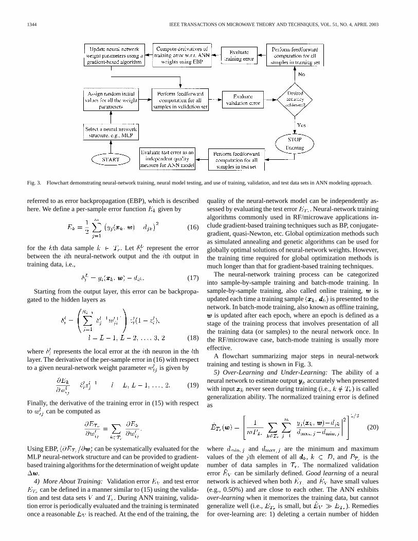
Fig. 3. Flowchart demonstrating neural-network training, neural model testing, and use of training, validation, and test data sets in ANN modeling approach.

referred to as error backpropagation (EBP), which is describedhere. We define a per-sample error functiongiven by

(16)

for the th data sample . Let represent the errorbetween the th neural-network output and theth output intraining data, i.e.,

(17)

Starting from the output layer, this error can be backpropa-gated to the hidden layers as

(18)

where represents the local error at theth neuron in thethlayer. The derivative of the per-sample error in (16) with respectto a given neural-network weight parameter is given by

(19)

Finally, the derivative of the training error in (15) with respectto can be computed as

Using EBP, can be systematically evaluated for theMLP neural-network structure and can be provided to gradient-based training algorithms for the determination of weight update

.4) More About Training: Validation error and test error

can be defined in a manner similar to (15) using the valida-tion and test data sets and . During ANN training, valida-tion error is periodically evaluated and the training is terminatedonce a reasonable is reached. At the end of the training, the

quality of the neural-network model can be independently as-sessed by evaluating the test error . Neural-network trainingalgorithms commonly used in RF/microwave applications in-clude gradient-based training techniques such as BP, conjugate-gradient, quasi-Newton, etc. Global optimization methods suchas simulated annealing and genetic algorithms can be used forglobally optimal solutions of neural-network weights. However,the training time required for global optimization methods ismuch longer than that for gradient-based training techniques.

The neural-network training process can be categorizedinto sample-by-sample training and batch-mode training. Insample-by-sample training, also called online training,isupdated each time a training sample is presented to thenetwork. In batch-mode training, also known as offline training,

is updated after each epoch, where an epoch is defined as astage of the training process that involves presentation of allthe training data (or samples) to the neural network once. Inthe RF/microwave case, batch-mode training is usually moreeffective.

A flowchart summarizing major steps in neural-networktraining and testing is shown in Fig. 3.

5) Over-Learning and Under-Learning:The ability of aneural network to estimate output accurately when presentedwith input never seen during training (i.e., ) is calledgeneralization ability. The normalized training error is definedas

(20)

where and are the minimum and maximumvalues of the th element of all , , and is thenumber of data samples in . The normalized validationerror can be similarly defined.Good learningof a neuralnetwork is achieved when both and have small values(e.g., 0.50%) and are close to each other. The ANN exhibitsover-learningwhen it memorizes the training data, but cannotgeneralize well (i.e., is small, but ). Remediesfor over-learning are: 1) deleting a certain number of hidden


neurons or 2) adding more samples to the training data. Theneural network exhibitsunder-learning, when it has difficultiesin learning the training data itself (i.e., ). Possibleremedies are: 1) adding more hidden neurons or 2) perturbingthe current solution to escape from a local minimum of

, and then continuing training.6) Quality Measures:The quality of a trained neural-net-

work model is evaluated with an independent set of data, i.e.,. We define a relative error for the th output of the neural

model for the th test sample as

(21)

A quality measure based on theth norm is then defined as

(22)

The average test error can be calculated usingas

Average Test Error (23)

where represents number of samples in test set. Theworst case error among all test samples and all neural-networkmodel outputs can be calculated using

(24)

Other statistical measures such as correlation coefficient andstandard deviation can also be used.

IV. COMPONENTMODELING USING NEURAL NETWORKS

Component/device modeling is one of the most importantareas of RF/microwave CAD. The efficiency of CAD tools de-pends largely on speed and accuracy of the component models.Development of neural-network models for active devices, pas-sive components, and high-speed interconnects has already beendemonstrated [6], [8], [24]. These neural models could be usedin device level analysis and also in circuit/system-level design[10], [12]. In this section, neural-network modeling examplesare presented in each of the above-mentioned categories.

A. High-Speed Interconnect Network

In this example, a neural network was trained to model signalpropagation delays of a VLSI interconnect network in printedcircuit boards (PCBs). The electrical equivalent circuit showingthe interconnection of a source integrated circuit (IC) pin tothe receiver pins is shown in Fig. 4. During PCB design, eachindividual interconnect network needs to be varied in termsof its interconnect lengths, receiver-pin load characteristics,source characteristics, and network topology. To facilitate this,a neural-network model of the interconnect configuration wasdeveloped [24].

The input variables in the model are, and .

Here, is length of the th interconnect, and areterminations of the th interconnect, is the sourceimpedance, and and are peak value and rise time of thesource voltage. The parameter identifies the interconnect

Fig. 4. Circuit representation of the VLSI interconnect network showing theconnection of a source IC pin to four receiver pins. A neural model is to bedeveloped to represent the signal delays at the four receiver pins as functions ofthe interconnect network parameters.

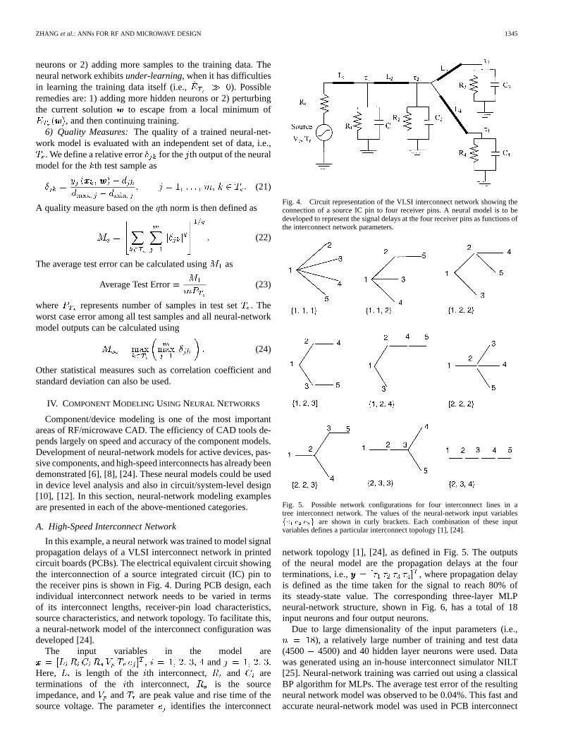
Fig. 5. Possible network configurations for four interconnect lines in atree interconnect network. The values of the neural-network input variablesfe e e g are shown in curly brackets. Each combination of these inputvariables defines a particular interconnect topology [1], [24].

network topology [1], [24], as defined in Fig. 5. The outputsof the neural model are the propagation delays at the fourterminations, i.e., , where propagation delayis defined as the time taken for the signal to reach 80% ofits steady-state value. The corresponding three-layer MLPneural-network structure, shown in Fig. 6, has a total of 18input neurons and four output neurons.

Due to large dimensionality of the input parameters (i.e.,), a relatively large number of training and test data

(4500 4500) and 40 hidden layer neurons were used. Datawas generated using an in-house interconnect simulator NILT[25]. Neural-network training was carried out using a classicalBP algorithm for MLPs. The average test error of the resultingneural network model was observed to be 0.04%. This fast andaccurate neural-network model was used in PCB interconnect


Fig. 6. Three-layer MLP structure with 18 inputs and four outputs used formodeling the interconnect network of Fig. 4.

simulation, where 20 000 interconnect trees (with differentinterconnect lengths, terminations, and topologies) had to berepetitively analyzed. Neural-model-based simulation wasobserved to be 310 times faster than existing NILT interconnectnetwork simulator. This enhanced model efficiency becomesimportant for the design of large VLSI circuits.

B. CPW Symmetric T-Junction

At microwave and millimeter-wave frequencies, CPW cir-cuits offer several advantages, such as the ease of shunt andseries connections, low radiation, low dispersion, and avoid-ance of the need for thin fragile substrates. Currently, CADtools available for CPW circuits are inadequate because of thenonavailability of fast and accurate models for CPW disconti-nuities such as T-junctions, bends, etc. Much effort has beenexpended in developing efficient methods for EM simulationof CPW discontinuities. However, the time-consuming natureof EM simulations limits the use of these tools for interactiveCAD, where the geometry of the component needs to be repet-itively changed, thereby necessitating massive EM simulations.Neural-network-based modeling and CAD approach addressesthis challenge.

In this example, the neural-network model of a symmetricT-junction [10] is described. The T-junction configuration issimilar to that of the 2T junction shown in Fig. 7. Variableneural model input parameters are the physical dimensions

, , , and , and the frequency of operation,i.e., . Parameters and

are strip width and gap dimension of the side CPW,where and specify the two colinear CPW lines.Air bridges shown in T-junctions of Fig. 7 are also includedfor the model development. The outputs of the ANN modelare the magnitudes and phases of the-parameters, i.e.,

.

Fig. 7. Geometry of the CPW folded double-stub filter circuit. Optimizationof the filter is carried out using fast EM-ANN models of various components inthe circuit.

TABLE IERRORCOMPARISONBETWEEN THEANN MODEL AND EM SIMULATIONS FOR

THE CPW SYMMETRIC T-JUNCTION. INPUT BRANCHLINE PORT ISPORT 1 AND

THE OUTPUT PORTS ON THEMAIN LINE ARE PORTS2 AND 3

Data generation was performed for 25 physical configurations(sizes) of the component over a frequency range of 1–50 GHz.The generated data was split into 155 training and 131 testsamples. A three-layer MLP neural-network structure with 15hidden layer neurons was trained using the BP algorithm. Theaccuracy of the developed neural models is shown in Table I interms of average error and standard deviation.

C. Transistor Modeling

Physics-based device models are CPU intensive, especiallywhen used for high-level design involving repetitive simula-tions. A neural-network model will be very efficient for this kindof devices in speeding up simulation and optimization. Two il-lustrative examples are presented for neural-network transistormodels.

In the first example, a neural-network model representinglarge-signal behavior of a MESFET was developed [12]. Theneural-network model has six inputs, i.e., gate length,gatewidth , channel thickness , doping density ,gate–source voltage , and drain–source voltage .Under normal operating conditions, the gate is reverse biasedand gate conduction current can be neglected. As a result,


Fig. 8. Comparison of small-signalS-parameter predictions from thelarge-signal MESFET neural-network model (o, +, x, �) with those from theKhatibzadeh and Trew MESFET model (—).

drain and source conduction currents and are equal.The neural-network model has four outputs including thedrain current and electrode charges, i.e., . Athree-layer MLP neural-network structure was used. Trainingand test data (a total of 1000 samples) were generated fromOSA903 simulations using a semianalytical MESFET modelby Khatibzadeh and Trew [26]. The neural network was trainedusing a modified BP algorithm including momentum adaptationto improve the speed of convergence. The trained neural modelaccurately predicted dc/ac characteristics of the MESFET.A comparison of the MESFET neural model’s-parameterpredictions versus those from the Khatibzadeh and TrewMESFET model is shown in Fig. 8. Since the neural modeldirectly describes terminal currents and charges as nonlinearfunctions of device parameters, it can be conveniently used forharmonic-balance simulations.

In the second example, neural-network models representingdc characteristics of a MOSFET were developed based onphysics-based data obtained by using a recent automatic modelgeneration algorithm [27]. The neural-network model has twoinputs, i.e., drain voltage and gate voltage . Draincurrent is the neural model output parameter. Trainingand test data were generated using a physics-basedMINIMOSsimulator.4 The average test errors of the trained MOSFETneural models were observed to be as low as 0.50%. Thisfast neural model of the MOSFET can, therefore, be used topredict the dc characteristics of the device with physics-basedsimulation accuracies.

V. CIRCUIT OPTIMIZATION USINGNEURAL-NETWORKMODELS

ANN models for RF/microwave components can be usedin circuit design and optimization. To achieve this, the neuralmodels are first incorporated into circuit simulators. Fordesigners who run the circuit simulator, the neural modelscan be used in a similar way as other models available in thesimulator’s library. An ANN model can be connected with

3OSA90, ver. 3.0, Optimization Syst. Associates, Dundas, ON, Canada (nowAgilent EEsof, Santa Rosa, CA).

4MINIMOS, ver. 6.1, Inst. Microelectron., Tech. Univ. Vienna, Vienna, Aus-tria.

other ANN models or with any other models in the simulatorto form a high-level circuit. In this section, circuit optimiza-tion examples utilizing fast and accurate neural models arepresented.

A. CPW Folded Double-Stub Filter

In this example, a CPW folded double-stub filter shown inFig. 7 was designed. For this design, the substrate parameters( , m, ) and the CPWparameters ( m, m) were fixed, yielding

. Fast neural-network models of CPW components,namely, the CPW transmission line, 90compensated bends,short-circuit stubs, and symmetric T-junctions (the one de-scribed in Section IV) were trained using accurate trainingdata from full-wave EM simulations. Design and optimizationof the filter were accomplished using theHP MDS5 networksimulator and the EM-ANN models of various components[10].

The filter was designed for a center frequency of 26 GHz.Ideally, the length of each short-circuit stub and the section ofline between the stubs should have a length of at 26 GHz.However, due to the presence of discontinuities, these lengthsneed to be adjusted. Parameters to be optimized areand . Initial values for these lengths were determined,and the corresponding structure showed a less than idealresponse when simulated. The circuit was then optimized,using gradient-descent, to provide the desired circuit response.The effect of optimization was a reduction in the two linelengths. A comparison of circuit responses using the initialEM-ANN design, optimized EM-ANN design, and full-waveEM simulation of the optimized filter circuit are shown inFig. 9. A good agreement was obtained between the EM-ANNand full-wave EM simulations of the optimized circuit overa frequency range of 1–50 GHz.

B. Three-Stage Monolithic-Microwave Integrated-Circuit(MMIC) Amplifier

In this example, MESFET neural models were used for yieldoptimization of a three-stage -band MMIC amplifier shownin Fig. 10. Component ANN models were incorporated into cir-cuit simulators AgilentADS6 andOSA90. Numerical results inthis example were from theOSA90implementation [12]. Thespecifications for the amplifier are as follows.

• Passband (8–12 GHz): 12.4 dBgain 15.6 dB, Inputvoltage standing-wave ratio (VSWR) 2.8.

• Stopband (less than 6 GHz and greater than 15 GHz): gain2 dB.

The ANN models of MESFETs (developed in Section IV) wereused in this amplifier design. There are 14 design variables, i.e.,metal-plate areas of the metal–insulator–metal (MIM) ca-pacitors , ) and number of turns of thespiral inductors ( , – ). A total of 37 statistical vari-ables including gate length, gatewidth, channel thickness, anddoping density of MESFET models, metal-plate area and thick-ness of capacitor models, and conductor width and spacing ofspiral inductor models were considered.

5MDS, Agilent Technol., Santa Rosa, CA.6ADS, Agilent Technol., Santa Rosa, CA.


Fig. 9. Comparison of the CPW folded double-stub filter responses beforeand after ANN-based optimization. A good agreement is achieved betweenANN-based simulations and full-wave EM simulations of the optimized circuit.

Fig. 10. A three-stage MMIC amplifier in which the three MESFETs arerepresented by neural-network models.

Yield optimization using an -centering algorithm [28] wasperformed with a minimax nominal design solution as the ini-tial point. The initial yield (before optimization) of the am-plifier using the minimax nominal design was 26% with fastANN-based simulations and 32% with relatively slow simula-tions using the Khatibzadeh and Trew MESFET models. Afteryield optimization using neural-network models, the amplifieryield improved from 32% to 58%, as verified by the MonteCarlo analysis using the original MESFET models. The MonteCarlo responses before and after yield optimization are shown inFig. 11. The use of neural-network models instead of the Khati-bzadeh and Trew models reduced the computation time for non-

(a) (b)

(c) (d)

Fig. 11. Monte Carlo responses of the three-stage MMIC amplifier. (a) and(b) Before yield optimization. (c) and (d) After yield optimization. Yieldoptimization was carried out using neural-network models of MESFETs.

linear statistical analysis and yield optimization from days tohours [12].

Considering that the Khatibzadeh and Trew models used inthis example for illustration purpose are semianalytical in na-ture, the CPU speed-up offered by neural-based design relativeto circuit design using physics-based semiconductor equationscould be even more significant.

VI. CONCLUSIONS

Neural networks have recently gained attention as a fast,accurate, and flexible tool to RF/microwave modeling, sim-ulation, and design. As this emerging technology expandsfrom university research into practical applications, there isa need to address the basic conceptual issues in ANN-basedCAD. Through this tutorial, we have tried to build a technicalbridge between microwave design concepts and neural-net-work fundamentals. Principal ideas in neural-network-basedtechniques have been explained to design-oriented readers ina simple manner. Neural-network model development frombeginning to end has been described with all the importantsteps involved. To demonstrate the application issues, a setof selected component modeling and circuit optimizationexamples have been presented. The ANN techniques arealso explained through a multimedia presentation includingnarrative audio clips (Appendix I) in the electronic versionof this paper on the CD-ROM accompanying this issue. Forthose readers interested in benefiting from neural networksright away, we have provided a hyperlink toNeuroModelerdemonstration software (Appendix II).

APPENDIX IMULTIMEDIA SLIDE PRESENTATION

A multimedia Microsoft PowerPoint slide presentation in-cluding narrative audio clips is made available to the readers


in the form of an Appendix. The presentation consisting of 55slides provides systematic highlights of the microwave-ANNmethodology and its practical applications. Some of the ad-vanced concepts are simplified using slide-by-slide illustrationsand animated transitions. The audio clips further help to makeself-learning of this emerging area easier.

APPENDIX IIHYPERLINK TO NeuroModelerSOFTWARE

A hyperlink to the demonstration version ofNeuroModelersoftware is provided. The software can be used to practice var-ious interesting concepts in the tutorial including neural-net-work structure creation, neural-network training, neural modeltesting, etc. The main purpose is to enable the readers to betterunderstand the neural-network-based design techniques and toget quick hands-on experience.

ACKNOWLEDGMENT

The authors thank L. Ton and M. Deo, both of the Departmentof Electronics, Carleton University, Ottawa, ON, Canada, fortheir help in preparing the multimedia Microsoft PowerPointslide presentation and this paper’s manuscript, respectively.

REFERENCES

[1] Q. J. Zhang and K. C. Gupta,Neural Networks for RF and MicrowaveDesign. Norwood, MA: Artech House, 2000.

[2] K. C. Gupta, “Emerging trends in millimeter-wave CAD,”IEEE Trans.Microwave Theory Tech., vol. 46, pp. 747–755, June 1998.

[3] V. K. Devabhaktuni, M. Yagoub, Y. Fang, J. Xu, and Q. J. Zhang,“Neural networks for microwave modeling: Model developmentissues and nonlinear modeling techniques,”Int. J. RF MicrowaveComputer-Aided Eng., vol. 11, pp. 4–21, 2001.

[4] V. K. Devabhaktuni, M. Yagoub, and Q. J. Zhang, “A robust algorithmfor automatic development of neural-network models for microwaveapplications,” IEEE Trans. Microwave Theory Tech., vol. 49, pp.2282–2291, Dec. 2001.

[5] V. K. Devabhaktuni, C. Xi, F. Wang, and Q. J. Zhang, “Robust trainingof microwave neural models,”Int. J. RF Microwave Computer-AidedEng., vol. 12, pp. 109–124, 2002.

[6] F. Wang and Q. J. Zhang, “Knowledge-based neural models for mi-crowave design,”IEEE Trans. Microwave Theory Tech., vol. 45, pp.2333–2343, Dec. 1997.

[7] F. Wang, V. K. Devabhaktuni, and Q. J. Zhang, “A hierarchical neuralnetwork approach to the development of a library of neural models formicrowave design,”IEEE Trans. Microwave Theory Tech., vol. 46, pp.2391–2403, Dec. 1998.

[8] P. M. Watson and K. C. Gupta, “EM-ANN models for microstrip viasand interconnects in dataset circuits,”IEEE Trans. Microwave TheoryTech., vol. 44, pp. 2495–2503, Dec. 1996.

[9] J. W. Bandler, M. A. Ismail, J. E. Rayas-Sanchez, and Q. J. Zhang,“Neuromodeling of microwave circuits exploiting space-mapping tech-nology,” IEEE Trans. Microwave Theory Tech., vol. 47, pp. 2417–2427,Dec. 1999.

[10] P. M. Watson and K. C. Gupta, “Design and optimization of CPW cir-cuits using EM-ANN models for CPW components,”IEEE Trans. Mi-crowave Theory Tech., vol. 45, pp. 2515–2523, Dec. 1997.

[11] G. L. Creech, B. J. Paul, C. D. Lesniak, T. J. Jenkins, and M. C. Calcatera,“Artificial neural networks for fast and accurate EM-CAD of microwavecircuits,” IEEE Trans. Microwave Theory Tech., vol. 45, pp. 794–802,May 1997.

[12] A. H. Zaabab, Q. J. Zhang, and M. S. Nakhla, “A neural networkmodeling approach to circuit optimization and statistical design,”IEEETrans. Microwave Theory Tech., vol. 43, pp. 1349–1358, June 1995.

[13] Y. Fang, M. Yagoub, F. Wang, and Q. J. Zhang, “A new macromodelingapproach for nonlinear microwave circuits based on recurrent neural net-works,” IEEE Trans. Microwave Theory Tech., vol. 48, pp. 2335–2344,Dec. 2000.

[14] J. Xu, M. Yagoub, R. Ding, and Q. J. Zhang, “Neural-based dynamicmodeling of nonlinear microwave circuits,”IEEE Trans. MicrowaveTheory Tech., vol. 50, pp. 2769–2780, Dec. 2002.

[15] M. Vai and S. Prasad, “Microwave circuit analysis and design by a mas-sively distributed computing network,”IEEE Trans. Microwave TheoryTech., vol. 43, pp. 1087–1094, May 1995.

[16] M. Vai, S. Wu, B. Li, and S. Prasad, “Reverse modeling of microwavecircuits with bidirectional neural network models,”IEEE Trans. Mi-crowave Theory Tech., vol. 46, pp. 1492–1494, Oct. 1998.

[17] J. A. Jargon, K. C. Gupta, and D. C. DeGroot, “Applications of artifi-cial neural networks to RF and microwave measurements,”Int. J. RFMicrowave Computer-Aided Eng., vol. 12, pp. 3–24, 2002.

[18] P. M. Watson, C. Cho, and K. C. Gupta, “Electromagnetic-artifi-cial neural network model for synthesis of physical dimensions formultilayer asymmetric coupled transmission structures,”Int. J. RFMicrowave Computer-Aided Eng., vol. 9, pp. 175–186, 1999.

[19] F. Wang, V. K. Devabhaktuni, C. Xi, and Q. J. Zhang, “Neural networkstructures and training algorithms for microwave applications,”Int. J.RF Microwave Computer-Aided Eng., vol. 9, pp. 216–240, 1999.

[20] K. Hornik, M. Stinchcombe, and H. White, “Multilayer feedforwardnetworks are universal approximators,”Neural Networks, vol. 2, pp.359–366, 1989.

[21] T. Y. Kwok and D. Y. Yeung, “Constructive algorithms for structurelearning in feedforward neural networks for regression problems,”IEEETrans. Neural Networks, vol. 8, pp. 630–645, May 1997.

[22] J. de Villiers and E. Barnard, “Backpropagation neural nets with one andtwo hidden layers,”IEEE Trans. Neural Networks, vol. 4, pp. 136–141,Jan. 1992.

[23] G. Thimm and E. Fiesler, “High-order and multilayer perceptron initial-ization,” IEEE Trans. Neural Networks, vol. 8, pp. 349–359, Mar. 1997.

[24] A. Veluswami, M. S. Nakhla, and Q. J. Zhang, “The application of neuralnetworks to EM-based simulation and optimization of interconnects inhigh-speed VLSI circuits,”IEEE Trans. Microwave Theory Tech., vol.45, pp. 712–723, May 1997.

[25] R. Griffith and M. S. Nakhla, “Time-domain analysis of lossy coupledtransmission lines,”IEEE Trans. Microwave Theory Tech., vol. 38, pp.1480–1487, Oct. 1990.

[26] M. A. Khatibzadeh and R. J. Trew, “A large-signal, analytical model forthe GaAs MESFET,”IEEE Trans. Microwave Theory Tech., vol. 36, pp.231–239, Feb. 1988.

[27] V. K. Devabhaktuni, B. Chattaraj, M. Yagoub, and Q. J. Zhang, “Ad-vanced microwave modeling framework exploiting automatic modelgeneration, knowledge neural networks, and space mapping,” inProc.IEEE MTT-S Int. Microwave Symp., Seattle, WA, 2002, pp. 1097–1100.

[28] J. W. Bandler and S. H. Chen, “Circuit optimization: The state of the art,”IEEE Trans. Microwave Theory Tech., vol. 36, pp. 424–443, MONTH1988.

Qi-Jun Zhang (S’84–M’87–SM’95) receivedthe B.Eng. degree from East China EngineeringInstitute, Nanjing, China, in 1982, and the Ph.D.degree in electrical engineering from McMasterUniversity, Hamilton, ON, Canada, in 1987.

He was with the System Engineering Institute,Tianjin University, Tianjin, China, in 1982 and1983. During 1988–1990, he was with OptimizationSystems Associates Inc. (OSA), Dundas, ON,Canada, developing advanced microwave optimiza-tion software. In 1990, he joined the Department of

Electronics, Carleton University, Ottawa, ON, Canada, where he is presently aProfessor. His research interests are neural network and optimization methodsfor high-speed/high-frequency circuit design, and has authored more than150 papers on these topics. He is a coauthor ofNeural Networks for RFand Microwave Design( Boston, MA: Artech House, 2000), a Co-Editor ofModeling and Simulation of High-Speed VLSI Interconnects(Boston, MA:Kluwer, 1994), and a contributor toAnalog Methods for Computer-AidedAnalysis and Diagnosis( New York: Marcel Dekker, 1988). He was a GuestCo-Editor for a Special Issue on High-Speed VLSI Interconnects of theInternational Journal of Analog Integrated Circuits and Signal Processingandtwice a Guest Editor for the Special Issues on Applications of ANN to RFand Microwave Design for theInternational Journal of Radio Frequency andMicrowave Computer-Aided Engineering.

Dr. Zhang is a member of the Professional Engineers of Ontario, Canada.


Kuldip C. Gupta (M’62–SM’74–F’88) received theB.Sc. degree in physics, math, and chemistry fromPunjab University, Punjab, India, in 1958, the B.E.and M.E. degrees in electrical communication engi-neering from the Indian Institute of Science, Banga-lore, India, in 1961 and 1962, respectively, and thePh.D. degree from the Birla Institute of Technologyand Science, Pilani, India, in 1969.

Since 1983, he has been a Professor with theUniversity of Colorado at Boulder. He is alsocurrently the Associate Director for the National

Science Foundation (NSF) Industry/University Cooperative Research (I/UCR)Center for Advanced Manufacturing and Packaging of Microwave, Opticaland Digital Electronics (CAMPmode), University of Colorado at Boulder,and a Guest Researcher with the RF Technology Group, National Institute ofStandards and Technology (NIST), Boulder, CO. From 1969 to 1984, he waswith the Indian Institute of Technology (IITK), Kanpur, India, where he was aProfessor of electrical engineering. From 1971 to 1979, he was the Coordinatorfor the Phased Array Radar Group, Advanced Center for Electronics Systems,Indian Institute of Technology. While on leave from the IITK, he was a VisitingProfessor with the University of Waterloo, Waterloo, ON, Canada, the EcolePolytechnique Federale de Lausanne, Lausanne, Switzerland, the TechnicalUniversity of Denmark, Lyngby, Denmark, the Eidgenossische TechnischeHochschule, Zurich, Switzerland, and the University of Kansas, Lawrence.From 1993 to 1994, while on sabbatical from the University of Coloradoat Boulder, he was a Visiting Professor with the Indian Institute of Scienceand a consultant with the Indian Telephone Industries. His current researchinterests are the areas of CAD techniques (including ANN applications) formicrowave and millimeter-wave ICs, nonlinear characterization and modeling,RF microelectromechanical systems (MEMS), and reconfigurable antennas. Hehas authored or coauthoredMicrowave Integrated Circuits(New York: Wiley,1974; New York: Halsted Press (of Wiley), 1974),Microstrip Line and Slotlines(Norwood, MA: Artech House, 1979; revised 2nd edition, 1996),Microwaves(New York: Wiley, 1979; New York: Halsted Press (of Wiley), 1980, MexicoCity, Mexico: Editorial Limusa Mexico, 1983),CAD of Microwave Circuits(Norwood, MA: Artech House, 1981, Beijing, China: Chinese ScientificPress, 1986, Moscow, Russia: Radio I Syvaz, 1987),Microstrip AntennaDesign(Norwood, MA: Artech House, 1988),Analysis and Design of PlanarMicrowave Components(Piscataway, NJ: IEEE Press, 1994),Analysis andDesign of Integrated Circuit-Antenna Modules(New York: Wiley 1999),andNeural Networks for RF and Microwave Design(Norwood, MA: ArtechHouse 2000). He has also contributed chapters to theHandbook of MicrostripAntennas(Stevenage, U.K.: Peregrinus, 1989), theHandbook of Microwaveand Optical Components, Volume 1(New York: Wiley, 1989),MicrowaveSolid State Circuit Design(New York: Wiley, 1988; 2nd edition 2003),Numerical Techniques for Microwave and Millimeter Wave Passive Structures(New York: Wiley, 1989), and theEncyclopedia of Electrical and ElectronicsEngineering(New York: Wiley, 1999). He has also authored or coauthoredover 230 research papers. He holds four patents in the microwave area. Heis the Founding Editor of theInternational Journal of RF and MicrowaveComputer-Aided Engineering, which is published by Wiley since 1991. He ison the Editorial Board ofMicrowave and Optical Technology Letters(Wiley),and theInternational Journal of Numerical Modeling(Wiley). He is listed inWho’s Who in America, Who’s Who in the World, Who’s Who in Engineering,andWho’s Who in American Education.

Dr. Gupta is a Fellow of the Institution of Electronics and TelecommunicationEngineers (India), a member of URSI (Commission D, U.S.), and a member ofthe Electromagnetics Academy (Massachusetts Institute of Technology (MIT),Cambridge). He is a member of the Administrative Committee (AdCom) forthe IEEE Microwave Theory and Techniques Society (IEEE MTT-S), chair ofthe IEEE MTT-S Standing Committee on Education, past co-chair of the IEEEMTT-S Technical Committee on Computer-Aided Design (MTT-1), a memberof the IEEE Technical Committee on Microwave Field Theory (MTT-15), anearlier member of the IEEE-EAB Committee on Continuing Education and theIEEE-EAB Societies Education Committee. He is an associate editor forIEEEMicrowave Magazineand is on the Editorial Board of the IEEE TRANSACTIONS

ON MICROWAVE THEORY AND TECHNIQUES. He was a recipient of the IEEEThird Millennium Medal and the IEEE MTT-S Distinguished Educator Award.

Vijay K. Devabhaktuni (S’97) received the B.Eng.degree in electrical and electronics engineering andthe M.Sc. degree in physics from the Birla Instituteof Technology and Science, Pilani, Rajasthan, India,in 1996, and is currently working toward the Ph.D.degree in electronics at Carleton University, Ottawa,ON, Canada.

He is currently a Sessional Lecturer with theDepartment of Electronics, Carleton University. Hisresearch interests include ANNs, computer-aided-design methodologies for VLSI circuits, and RF

and microwave modeling techniques.Mr. Devabhaktuni was the recipient of a 1999 Best Student Research

Exhibit Award presented by Nortel Networks. He was a two-time recipientof the Ontario Graduate Scholarship for the 1999–2000 and 2000–2001academic years presented by the Ministry of Education and Training,ON, Canada. He was the recipient of the 2001 John Ruptash MemorialFellowship, which is awarded annually to an outstanding graduate student ofthe Faculty of Engineering, Carleton University. He was also the recipientof the 2001 Teaching Excellence Award in Engineering presented by theCarleton University Student’s Association.

artificial neural networks for rf and microwave design-from theory to

Documents