article: an overview of the risk-neutral valuation of bank ... · consequently, the cds premium...

EY Global Financial Services Institute July 2015 | Volume 3 – Issue 2

The Journal of Financial Perspectives

Article:An overview of the risk-neutral valuation of bank loans

An overview of the risk-neutral valuation of bank loansDanilo TillocaVice President, Group Special Entities Risk and Evaluation, Unicredit Holding SpA

Luciano TuzziSenior Vice President, Head of Group Special Entities Risk and Evaluation,Unicredit Holding SpA

1

AbstractThis paper provides an overview of a new methodology that allows banks to evaluate loans using the risk-neutral approach. In specifically, it illustrates the methodological framework behind the definition of the risk-neutral default probabilities used to estimate the loans credit spreads. These risk-neutral probabilities are calculated using a contingent-claims approach conceptually similar to the Black–Scholes and Merton framework for modeling corporate liabilities. The proposed risk-neutral approach is suitable for producing estimates, in a fair value computation context, that are as close as possible to the “exit price,” as mandated by IFRS 13, with a lower dependency on internal parameters.

https://gfsi.ey.com/

https://twitter.com/intent/tweet?text=An%20overview%20of%20the%20risk-neutral%20valuation%20of%20bank%20loans&url=https://www.gfsi.ey.com/the-journal-x.php?pid=13&id=101

https://www.facebook.com/sharer/sharer.php?u=https://www.gfsi.ey.com/the-journal-x.php?pid=13&id=101

https://www.linkedin.com/shareArticle?mini=true&url=https://www.gfsi.ey.com/the-journal-x.php?pid=13&id=101

https://www.gfsi.ey.com/the-journal-x.php?pid=13&id=101 &loc=EmailArticle

An overview of the risk-neutral valuation of bank loans

1. Theoretical framework1.1 Risk-neutral pricing overviewThe introduction of IFRS 13, at the beginning of 2013, required, inter alia, that fair value measurements made for disclosure purposes1 should maximize observable market data by minimizing the usage of unobservable and entity specific inputs. Given these requirements, a new approach is proposed in this article, based on the contingent-claims framework for the pricing of bank loans. The problem of evaluating risky debt using contingent-claims approaches has been addressed by many researchers in literature, as a result of which we have had a proliferation of complex models, most of which have paid little attention to the practical applicability of the models [Bohn (2000)]. The proposed approach tries to balance between simplicity and usefulness by providing a tractable, but realistic, approach to loan fair value estimation. We hope that the model proposed here would contribute toward defining a new standard in the banking industry for IFRS 13 compliant valuation of loans.

Prior to the introduction of IFRS 13, bank loans were usually evaluated using the real-world internal default probabilities and a certain number of other internal parameters, such as the bank’s cost of equity, credit VaR, administrative costs and internal transfer rate.2 After the introduction of IFRS 13, banks were required to replace the old internally focused approach with a new model that used parameters linked to observable market inputs, moving to the so-called risk-neutral approach.

The problem, of course, is that very few bank loan transactions are observable on the market. Consequently, even if the discount methodology used to evaluate the loans is similar to the one used for pricing the debentures, it is not usually possible to apply the same spreads, making it necessary to find a link between observed market spreads and bank loans (even if the latter are not traded). To solve this problem, the proposed methodology assumes that bonds and loans have the same market risk premia in common.

1 Loans and receivables with banks and customers, debt securities held to maturity, liabilities due to banks and customers and issued bonds. 2 Given that there wasn’t any industry-wide accepted methodology, the internal parameters differed from

one bank to another.

2







This assumption, which has its foundation in the Capital Asset Pricing Model (CAPM) theory, allows us to transform, through a correlation factor, the market risk premium into a loan-specific risk premium. In effect, if one accepts that the observed market spreads incorporate the market risk premium, then it is reasonable to assume that the loans prices, if quoted on the market, should incorporate, in some way, the same premium. From an operational standing point, it is necessary to take into account the differences and specificities that arise when comparing observed market spreads with specific loan characteristic and debtor creditworthiness.

The proposed model addresses this issue by using the contingent-claims model for the evaluation of risky debt, based on the pioneering work of Black, Sholes and Merton (BSM). Using this approach, we find that there is a link between the real-world default probabilities, which is used to measure the creditworthiness of a debtor, and the risk-neutral one (observed and embedded in the market spreads), and that this link is a function of the market risk premium, also called “the Sharpe ratio.” The proposed methodology bases its estimates on the calibration of the Sharpe ratio using quotes observed in the most advantageous credit market. The estimated fair value calculated in this way aims to determine the exit price in these markets.

The market price of risk estimated in this way reflects all the factors that a market participant would consider when pricing the asset or liability, such as the default probability, recovery rate and funding costs.

In this paper, it is assumed that, if the loans evaluated using the proposed approach were listed on an active market, they would be subject to the same market price of risk as the ones observed on the public markets. In other words, there is no need for additional illiquidity premiums, just as IFRS 13 had mandated.

3







1.2 The relationship between real-word probabilities and risk-neutral probabilitiesWe use the Merton (1974) approach to define the relationship between the real-world default probabilities (PD) and the risk-neutral ones. Following Black and Cox (1976), we assume as given the exogenous insolvency trigger; when this trigger is reached, all the outstanding debt is assumed to default and the investor will recover a given amount “R”. Under these hypotheses, it is possible show that the cumulative risk-neutral default probability CDPR is linked to the real-world CDPW through the Sharpe ratio (λi), which measures the excess return per unit of risk. Since the Sharpe ratio of the asset under evaluation will usually differ from the Sharpe ratio of the market, we have to use the CAPM model to express the specific λi of the asset under evaluation, in terms of the market risk premium (λm). The asset-specific risk premium is the market-specific risk premium adjusted by the correlation between the asset and the market. In particular, the calibration of risk-neutral PDs is conceived within a sector-specific context that aims to estimate sector-specific market parameters. Under this approach, λm is substitute by λs, and the asset-specific Sharpe ratio is given by the following relationship: λi=ρi,s·λs.

1.3 Default probability estimation from market quotes1.3.1 Estimation from credit default swapsThe cumulative PDs implied by the market can be derived from the CDS market quotes.3 CDSs are contracts that give the right and the obligation to be compensated for a loss, given the default of a reference entity. The assurance premium for this kind of protection is paid in the form of a spread over the notional covered by the CDS contract. We can price the CDS using the difference between the fee-leg paid by the investor, which includes the premiums streams to compensate the protection seller, and the default-leg paid by the latter, which includes the payment of the loss in case of default of the reference entity. The estimation of the risk-neutral cumulative default probabilities can be performed using the full bootstrapping of the term structure of hazard rates.

3 To ensure that we avoid the impact of market-maker spread, which is not directly related to the creditworthiness of the entity, on our estimation of credit risk we will use the par-spread estimated from CDS mid-quotes.

4







1.3.2 Estimation from risky bondsUsing the prices of risky zero-coupon bonds, it is possible to estimate the implied market default probabilities.4 The market convention is to incorporate all the expectations regarding the default and recovery on the spread over the risk-free rate. Assuming that the expected loan recovery rate R is known, we can write the fair value formula in order to incorporate explicitly the cumulative default probability CDP(t), hence removing the need for using the credit spread. In effect, we know that, if the bond will not default, the investor will receive at the maturity t, 1 with probability S(t)=1-CDP(t), while in case of default the investor will receive the expected recovery R with marginal default probability

for every t#x (since it is unknown when the default will occur).

This relationship can be extended to coupon-bearing bonds, since in this case, the fair value can be expressed as a strip of zero coupons. Consequently, the bond–based approach applied to market PD estimation consists of the following two steps:

1. Spread computation: issuer-specific spread is estimated using the bond return and the swap curve of reference for the issuer selected.

2. Market CDP estimation: the CDP at time t implied by the market is estimated through a bootstrapping procedure.

With reference to loss given default (LGD), the issuer-specific parameter is typically estimated by the bank; however, if that is not available it is assumed to equal 60% (CDS market convention).

4 We are following an approach similar to the one proposed by Fons (1994), which can be considered as one of the first reduced-form models.

5







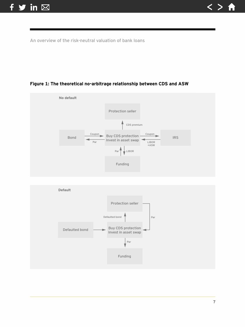
1.4 Relationship between CDS quotes and bonds spreadsThe proposed approach uses CDS quote spreads to estimate the credit risk premia, though it is also possible to estimate this premia using the credit spread paid on bonds.5 In the market, the difference between these spreads is referred to as CDS-bond basis6 and has been the subject of several studies. For example, Hull et al. (2005) demonstrated that, if the LIBOR curve is used as the risk-free curve when estimating the bond spread, the two spreads are almost equivalent. The reason for this equivalence is explained in Figure 1. The figure illustrates how, for investors that funds themselves at LIBOR, a combined position of buying protection in a CDS and entering into an asset swap in which the fixed-coupon payments of a bond that trades at par are swapped against a stream of floating rates, is fully hedged in any state of the world. Before maturity, there are two possibilities: no-default (left-hand side) and default (right-hand side, assuming physical delivery and unwinding of the IRS). In both cases, the combined position is credit risk-free.

Consequently, the CDS premium should match the asset swap spread. If the difference between the CDS premium and the asset swap spread were to diverge from zero, it would result in a theoretical arbitrage opportunity. If the CDS-bond basis becomes positive (negative), an arbitrageur will find it profitable to sell (to buy) the cash bond in an asset swap and to sell (to buy) CDS protection at the same time. In effect, the arbitrage is generally not perfect and there are a few technical reasons (difficulty in short-selling bonds, cheapest-to-deliver option) that tend to push the basis into the positive territory. In summary, the pre-crisis literature suggests that the arbitrage relationship between CDS and cash-bond spreads holds fairly well and that, if anything, the basis should be slightly positive. As a consequence of the 2007–08 financial crisis, this basis has become persistently negative.

5 From a practical point of view, we refer to the asset swap (ASW) spread since it is the simplest way of transforming a fixed-rate bond into a strip of floating cashflows plus spread.

6 We define this basis as: ParSpreadCDS — SpreadASW

6







Figure 1: The theoretical no-arbitrage relationship between CDS and ASW

No default

Protection seller

Funding Funding

Buy CDS protectionInvest in asset swap


BondPar

Coupon Coupon

Par Par

Par

LIBOR

CDS premium Defaulted bond

LIBOR+ASW

IRS Defaulted bond

Default

Protection seller

7

No default

Protection seller

Funding Funding



BondPar

Coupon Coupon

Par Par

Par

LIBOR

CDS premium Defaulted bond

LIBOR+ASW

IRS Defaulted bond

Default

Protection seller







In order to exploit the negative basis, an arbitrageur would have to finance the purchase of the underlying bond and buy protection. During the credit crisis, because of funding liquidity shortage and increased risk in the financial institutions, closing this gap became more difficult, risky and expensive. During the financial crisis, the negative basis was stable and persistent; in effect, the basis trading was facing liquidity and counterparty risk, and hence was not risk-free.7

We conclude by stating that, in normal market conditions, we can consider the CDS quotes and bond spreads interchangeable for the estimation of credit risk premia. However, since during stress times, asset prices depart from frictionless ideals (due to funding liquidity risk faced by the financial institutions and investors), the CDS quotes should be preferred in order to avoid embedding in the estimation factors that are not strictly related to the credit risk.8

2. Calibration methodologyAs suggested, the definition of risk-neutral cumulative default probabilities lies on the correct and consistent calibration of the market parameters. To this extent, the present calibration methodology illustrates the procedure to consistently estimate the market-specific risk premium ( ). In specifically, the calibration methodology uses historical cumulative PDs, issuer-specific correlations ( ) and market PDs as input data to ultimately estimate market-specific risk premium ( ). By minimizing the estimation error on the market quotes, the proposed methodology maximizes the market information embedded in these values. The proposed calibration methodology also provides stable estimates, since the final values are obtained using an average of the last 250 estimates and hence is able to absorb the daily volatility of quotations.

7 The analysis of this basis and of 2007/08 financial crisis is beyond the scope of this paper. More details and a complete bibliography can be found in Augustin (2012). 8 In situations where there is a persistent (not temporary) negative CDS-bond basis, it might be necessary

to consider it as an additional liquidity premium for the funded loans market and incorporate it in the loans discount spread.

8







2.1 Sample portfolioIt is necessary to define a sample portfolio in order to estimate the market risk parameter ( ) in a sector- and region-specific context. This means that, for every country where this methodology is applied, it will be necessary to estimate the country-specific lambdas sectors.

2.2 Input data2.2.1 Market PDs As described in section 1.3 , the market cumulative PDs can be derived from the CDS market quotes or from the bonds prices observed on the market.

2.2.2 Internal PDs The issuer-specific internal cumulative probabilities of default are the physical default probabilities usually adopted by banks to perform internal evaluation of loans. It is important to stress the concept that, due to the way we calibrate and transform the real-world probabilities, the proposed approach is robust to misspecification of this parameter. Berg and Kaserer (2009) demonstrated that the market risk premia estimation is particularly robust when applied to the five-year bucket.9

2.2.3 Rho The correlation parameter can be defined on either a specific-issuer or sector-specific basis. In the CAPM, this parameter represents the correlation between the issuer’s assets and market returns. Instead of the CAPM, a more sophisticated factor model can be used to determine the sensitivity of the default probability of the issuer to certain risk factors. In particular, it is possible to model the single issuer creditworthiness as a function of both the cluster the issuer belongs to and obligor-specific credit risk.

9

9 The authors showed that, in the CDS market, the five-year maturity is the most liquid and that trades during periods of turmoil tend to concentrate to this maturity.







2.3 Market price of risk calibration As suggested, market-specific risk premium represents the expected excess return demanded by investors per unit of risk. This parameter is estimated through a calibration where is calculated as the average of daily λ(t) estimations. According to this approach,

is calculated through the following process:

• Estimation of the daily (t) individual market CDPM for every issuer i in the sample.

• Estimation of daily individual expected CDP for the issuer i.

• is, ultimately, calculated as the arithmetic average of the daily observed .

In order to make the estimate as specific as possible, a different parameter is estimated for every sector — financial, large corporate and government. The estimates are run over a time horizon suitable at guaranteeing a consistent calibration in terms of both asset liquidity and number of observations.10

3. Formula behaviorIn this section, we will provide more information about the “fair value” loan formula and, in particular, on its behavior and applicability in the credit market. As the source for the real-world default probabilities, we will use “Global corporate average cumulative default rates” (CDR), published by Standard & Poor’s [Vazza et al. (2012)], and for historical CDS quotes, we will use the Markit sector curves composite, calculated using the methodology applied by Markit (2012).

3.1 The fair value loan formulaIt is possible to extend the pricing of risky zero-coupon bonds to loans pricing by substituting the bond coupons with the loan cashflows. However, it is important to note that the LGD for loans is calculated only on the outstanding debt; hence, in the case of default, it is assumed that the recovery of remaining interest coupons is zero. This implies that, for pricing purposes, the loan cashflow needs to be split into two components: the repaid notional and the paid interests.

10

10 A time horizon that could be used as reference is around 250 observations.







3.2 Negative risk-neutral PDsTheoretically, it is possible that, during calibration, we estimate negative market risk premiums. This fact could pose problems during the transformation from real-world PDs to risk-neutral PDs, since we could obtain risk-neutral PDs that decrease over the time. We know that this is not possible in the real world, and we expect that this would also be the case in a risk-neutral world.

From a theoretical point of view, the risk-neutral world is one wherein the expected return required by all investors on all investments is the risk-free interest rate. It is then theoretically possible that, if the investors’ assumptions on the riskiness are wrong and too optimistic, to move from the real world to this world, the market risk premium could be constrained to become negative.

Looking at historical CDS quotes, we have observed that, in certain circumstances, the market risk premium is negative. We have observed this behavior from the CDS quotes related to issues rated B from the period January 2013 to December 2013 (see the left-hand panel of Figure 2). To determine the accuracy of our findings, we also tested our hypothesis using the spread of Bloomberg’s composite of U.S. issues rated B (see the right-hand panel of Figure 2). Both analyses provide evidence in support of the proposition that B-rated short-term debt (years 1–3) has an implied negative market risk premium.

11







Since the information regarding the historical defaults, for this class of loans, is publicly available to all the investors, the question that arises is why investors ignore this information. Our conclusion is that the observed behavior is probably due to the fact that, in a low interest rate regime, investors who are looking for higher yields are willing to invest in short-term sub-grade loans. This has the effect of lowering the market-implied default probability. Naturally, over the long term, the market risk premium turns into the positive territory. This example provides support for the proposition that real-world probabilities are different from the risk-neutral probabilities, since the latter are an expression of the forces driving the markets and could show implied default probabilities that could never be observed in the real world.

Our opinion is that, even if a negative market risk premium could theoretically be observed, this event can practically happen very rarely, and only in certain conditions (such as very low risk-free returns and short-term low investment grade debt). To understand the reasoning, it is important to note that the calibration process for the lambda estimation is performed only on market quotations of observable obligations quotes or CDS par spreads.

12

11 An approach followed, for example, to price the bank liabilities.

Per

cent

Lambda average

Term bucket Observation date

-1.0

0

0.5

1.0

1.5

2.0

2.5

3.0

Y1 Y2 Y3 Y4 Y5 Y7 Y10–1.0

–0.5

Feb

13

Apr

13

May

13

July

13

Sep

13

Nov

13

Dec

13

Jun 09 Jan 10 Jul 10 Feb 11 Aug 11 Mar 12 Oct 12 Apr 13 Nov 13 May 14

1Y

2Y

3Y

5Y

10Y

B lambda average (period: Jan 13–Dec 13) Daily lambda estimation Bloomberg FI composite rating B U.S.$

-0.5

0

0.5

1.0

2.0

3.0

3.5

4.0

1.5

2.5

Figure 2: Risk premium related to B-rated loans/securities







This implies that all the reference entities used for the calibration should have an agency rating. Since the internal models used by banks, for the estimation of default probability, is based on the shadow rating approach, the internal estimate of the PD should be near the agency one. Given that this information is publicly available, the market quotations should always imply a market PD higher than the internal PD estimate, since it should at least incorporate a premium for liquidity and recovery expectations [Turnbull (2003)]. In summary, an estimation of negative lambda should never happen, and if it does, it is probably a sign that the internal PD has been wrongly assigned. Before accepting it, the assigned rating should be verified. The positivity of the marginal PD should always be checked and confirmed to mitigate the risk of incorrectly assigning internal PDs. In case the credit spread of the loan counterpart can be inferred directly using market quotes of liquid instruments, it is possible to avoid the use of lambda and directly apply the default probabilities implied by the market spread.11

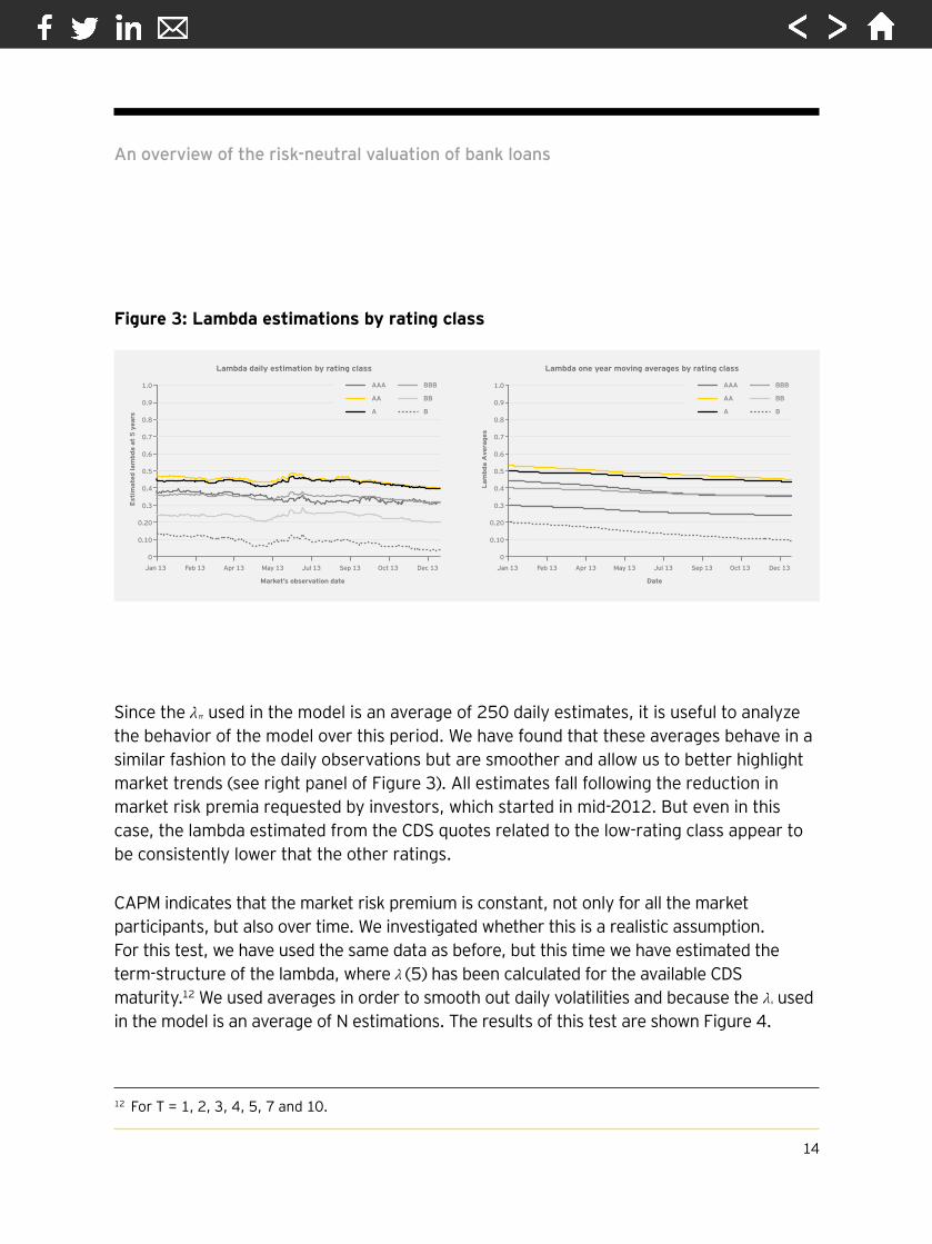
3.3 Constancy of the sector lambdaThe model assumes that we can keep constant the sector lambda sm for each counterpart belonging to a given sector. This assumption is a direct consequence of the CAPM, which indicates that the market risk premium is constant and equal for all the market participants. This means that the sm estimated from an AA counterpart can be applied to BBB or AAA counterparts. To verify this hypothesis, we have calculated the lambda from Markit generic sector curves to see if they are interchangeable. The CDPW has been taken from Vazza et al. (2013), while the term of the CDS quotes considered was five years (T=5). The results are shown in Figure 3.

We can observe that the estimated sm is not constant over the time, but that the differences are not very large, with the exception of those with a low rating (below BB rating). The results corroborate those of Berg (2010), who found that the term structure of the risk premia was flat before the 2007–08 crisis, and subsequently sloped downward during the crisis. Sadly, since that paper was published in 2010, it does not contain information about the period after the credit crisis. Our analysis, which covers a period of one to two years, shows that the term structure of risk premia is again becoming flat.

13







Since the used in the model is an average of 250 daily estimates, it is useful to analyze the behavior of the model over this period. We have found that these averages behave in a similar fashion to the daily observations but are smoother and allow us to better highlight market trends (see right panel of Figure 3). All estimates fall following the reduction in market risk premia requested by investors, which started in mid-2012. But even in this case, the lambda estimated from the CDS quotes related to the low-rating class appear to be consistently lower that the other ratings.

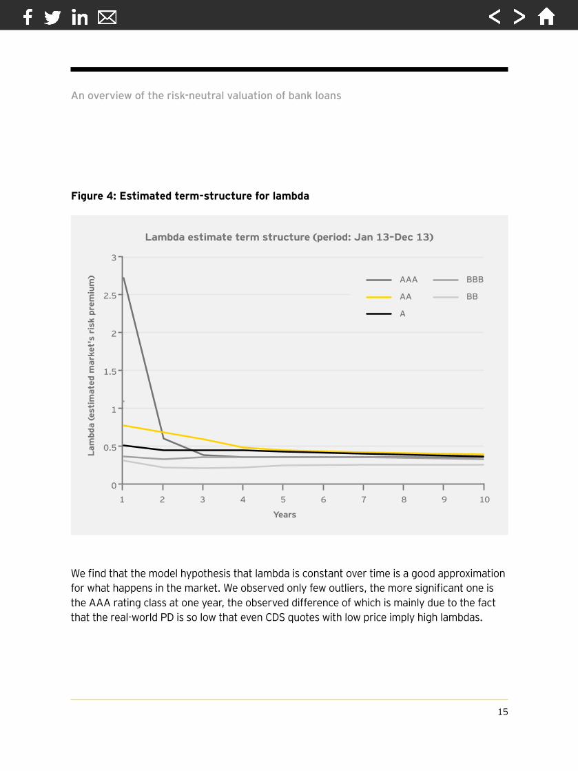
CAPM indicates that the market risk premium is constant, not only for all the market participants, but also over time. We investigated whether this is a realistic assumption. For this test, we have used the same data as before, but this time we have estimated the term-structure of the lambda, where (5) has been calculated for the available CDS maturity.12 We used averages in order to smooth out daily volatilities and because the sm used in the model is an average of N estimations. The results of this test are shown Figure 4.

14

0.6

Est

imat

ed la

mbd

a at

5 y

ears

Market’s observation date

0

0.10

0.20

0.3

0.4

0.6

0.9

1.0

0.5

0.8

0.7

Jan 13 Feb 13 Apr 13 May 13 Jul 13 Sep 13 Oct 13 Dec 13

AAA

AA

A

BBB

BB

B

Lambda daily estimation by rating class

Lam

bda

Ave

rage

s

Date

0

0.10

0.20

0.3

0.4

0.9

1.0

0.5

0.8

0.7

Jan 13 Feb 13 Apr 13 May 13 Jul 13 Sep 13 Oct 13 Dec 13

AAA

AA

A

BBB

BB

B

Lambda one year moving averages by rating class

Figure 3: Lambda estimations by rating class

12 For T = 1, 2, 3, 4, 5, 7 and 10.







We find that the model hypothesis that lambda is constant over time is a good approximation for what happens in the market. We observed only few outliers, the more significant one is the AAA rating class at one year, the observed difference of which is mainly due to the fact that the real-world PD is so low that even CDS quotes with low price imply high lambdas.

15

Lam

bda

(est

imat

ed m

arke

t's

risk

pre

miu

m)

Years

0

0.5

1

2.5

3

2

1.5

1 2 3 4 5 6 7 108 9

AAA

AA

A

BBB

BB

Lambda estimate term structure (period: Jan 13–Dec 13)

Figure 4: Estimated term-structure for lambda







To conclude this section, we want to stress that the default probabilities implied in the bond prices and CDS spreads (risk-neutral PDs) should always be higher than the real-world PDs. This fact was first highlighted by Altman (1989), who described the discrepancy between bond prices and historical default data. Elton et al. (2001) provided an in-depth analysis of the spread between rates on corporate and government bonds. The main reasons for such differences are the following:

1. The investors raise the expected returns they require on corporate bonds to compensate for their relatively low liquidity.

2. Bond traders are allowing, in their pricing, for the possibility of depressed scenarios much worse than anything seen during the time period covered by historical data. This occurs because a large part of the risk on corporate bonds is systematic rather than diversifiable.

Hence, we cannot expect risk-neutral PDs to converge toward internal PDs. In addition, the fact that this difference grows with the square root of time is a consequence of the assumption that the assets that could trigger a default, follow a log-normal geometric Brownian motion. This kind of assumption is used in many credit models, such as KMV [Agrawal et al. (2004)], and has been recently proposed by Berg and Kaserer (2009).

16

13 This fact was first highlighted by Berg and Kaserer (2009).







17

1

2

3

4

Credit market quotes Risk-free rates

Correction factor

Market risk premia(Sharpe ratio)

Loan risk premia

PD risk neutral (equivalent market PD)

Loan risk-neutral spread (equivalent market

spread)

Loan physical PD(bank internal PD)

Loss given default (collateral factor)

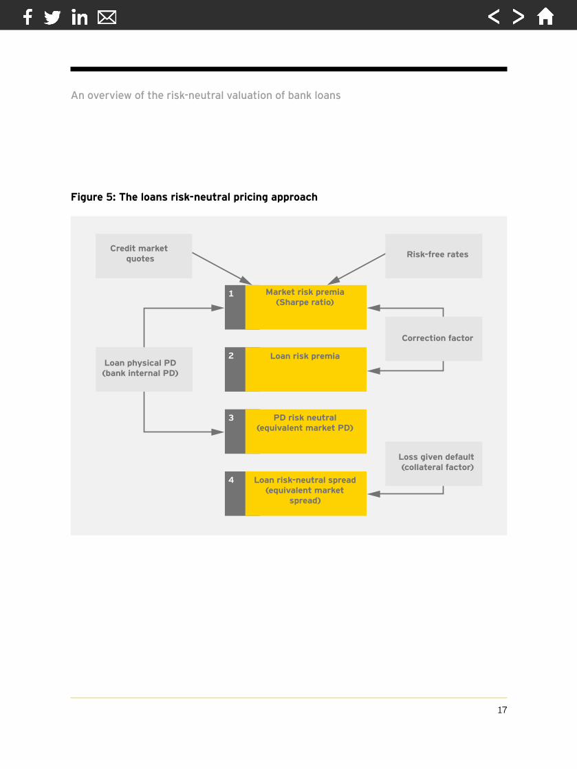
Figure 5: The loans risk-neutral pricing approach







4. ConclusionTo mark credit assets using a valuation model, it is necessary to estimate the risk-neutral default probabilities from the quotes observable in the credit market (such as bond prices and credit default swap spreads). Currently, two approaches to mark a credit asset to model are proposed in the literature: 1) the reduced-form approach, where it is assumed that the price of any security is the expected value of its future cashflows and 2) the structural approach, where the default occurs when the value of a firm’s assets declines below a given threshold. We believe that the two approaches are not mutually exclusive, but are complementary. In this article, the two approaches were combined in order to allow for the evaluation of a great variety and type of commercial loans. Both internal and external data are used for this purpose. The first approach has been used to build the discount methodology, while the second approach allowed us to extend the methodology, to those loans whose prices are not observable in the market.

We summarize the steps proposed in this paper for calculating the credit spread for loans pricing as follows (Figure 5):

1. Estimate of the market risk premia using the observed credit-market quotes.

2. Using the right correlation factor, calculate the specific risk premia of the loan under evaluation.

3. Knowing the physical default probability and the specific risk premia of the loan, it is possible to calculate the proper risk-neutral default probability.

4. Using a non-arbitrage approach that takes into account the loan collateral, it is possible to transform the risk-neutral PD into a proper credit spread suitable to be applied to discount the loan cashflows.

It is important to note that we have substituted most of the internal parameters with information obtained from the credit markets, and only left the LGD, correlation factor and real-world default probability to be derived from internal information. It is also important to highlight the fact that, due to the way in which the calibration and transformation of the real-world probabilities work, the proposed approach is robust to misspecification of this parameter.13

18







ReferencesAgrawal, D., N. Arora, and J. Bohn, 2004, “Parsimony in practice: an Edf-based model of credit spreads,” Moody’s KVM Publications, AprilAltman, E., 1989, “Measuring corporate bond mortality and performance,” Journal of Finance 44, 902–922Augustin, P., 2012, “Squeezed everywhere — can we learn something new from the CDS-bond basis ?” Working Paper on SSRNBerg, T., 2010, “The term structure of risk premia — new evidence from the financial crisis,” ECB Working Paper Series, no. 1165, MarchBerg, T., and C. Kaserer, 2009, “Estimating equity premia from CDS spreads,” EFA Working Paper SeriesBlack, F., and J. Cox, 1976, “Valuing corporate securities: some effects of bond indenture provisions,” Journal of Finance 31:2, 351–367Black, F., and M. Sholes, 1973, “The pricing of options and corporate liabilities,” Journal of Political Economy 81, 637–659Bohn, J., 2000, “A survey of contingent-claims approaches to risky debt valuation,” Journal of Risk Finance 1:3, 53–78Elton, E., M. Gruber, D. Agrawal, and C. Mann, 2001, “Explaining the rate spread on corporate bonds,” Journal of Finance 56:1, 247–77Fama, E., and K. French, 2004, “The Capital Asset Pricing Model: theory and evidence,” Journal of Economic Perspectives 18:3, 25–46Fons, J., 1994, “Using default rates to model the term structure of credit risk,” Financial Analysts Journal, 50, 25–33Hull, J., M. Predescu, and A. White, 2005, “Bond prices, default probabilities and risk premiums,” Journal of Credit Risk 1:2, 53–60Kealhofer, S., and M. Kurbat, 2002, “Predictive Merton models,” Risk, FebruaryMarkit, 2012, “Markit sector curves calculation methodology,” Markit Group Limited, FebruaryMerton, R., 1974, “On the pricing of corporate debt: the risk neutral structure of interest rates,” Journal of Finance 29, 449–470Turnbull, S. M., 2003, “Pricing loans using default probabilities,” Economic Notes, Banca Monte dei Paschi di Siena SpA 32:2, 197–217Vazza, D., N. Kraemer, and N. Richhariya, “2012 annual global corporate default study and rating transitions,” Standard & Poor’s Financial Services LLC

19






Editorial

Special Advisory EditorsBen GolubBlackRockAnthony NeohBank of ChinaSteve PerryVisa Europe

Antony M. SantomeroThe Wharton SchoolNick SilitchPrudential Financial

Editorial BoardViral V. Acharya New York UniversityJohn Armour University of OxfordPhilip Booth Cass Business School and IEAJosé Manuel CampaIESE Business SchoolKalok Chan Hong Kong University of Science and TechnologyJ. David Cummins Temple UniversityAllen Ferrell Harvard Law SchoolThierry Foucault HEC ParisRoland Füss University of St. GallenGiampaolo Gabbi SDA BocconiBoris Groysberg Harvard Business SchoolScott E. Harrington The Wharton SchoolJun-Koo Kang Nanyang Business School

Takao Kobayashi Aoyama Gakuin UniversityDeborah J. Lucas Massachusetts Institute of TechnologyMassimo Massa INSEADTim Morris University of OxfordPatrice Poncet ESSEC Business SchoolMichael R. Powers Tsinghua UniversityPhilip Rawlings Queen Mary, University of LondonRoberta Romano Yale Law SchoolHato Schmeiser University of St. GallenPeter SwanUniversity of New South WalesMarno Verbeek Erasmus UniversityBernard Yeung National University of Singapore

EditorShahin Shojai EY UAE

Advisory EditorsDai Bedford EY U.K.Shaun Crawford EY U.K.David Gittleson EY U.K.

Michael Inserra EY U.S. Michael Lee EY U.S.Bill Schlich EY U.S.

The EY Global Financial Services Institute brings together world-renowned thought leaders and practitioners from top-tier academic institutions, global financial services firms, public policy organizations and regulators to develop solutions to the most pertinent issues facing the financial services industry.

The Journal of Financial Perspectives aims to become the medium of choice for senior financial services executives from banking and capital markets, wealth and asset management and insurance, as well as academics and policymakers who wish to keep abreast of the latest ideas from some of the world’s foremost thought leaders in financial services. To achieve this objective, a board comprising leading academic scholars and respected financial executives has been established to solicit articles that not only make genuine contributions to the most important topics, but are also practical in their focus. The Journal will be published three times a year.

gfsi.ey.com

About EYEY is a global leader in assurance, tax, transaction and advisory services. The insights and quality services we deliver help build trust and confidence in the capital markets and in economies the world over. We develop outstanding leaders who team to deliver on our promises to all of our stakeholders. In so doing, we play a critical role in building a better working world for our people, for our clients and for our communities.

EY refers to the global organization, and may refer to one or more, of the member firms of Ernst & Young Global Limited, each of which is a separate legal entity. Ernst & Young Global Limited, a UK company limited by guarantee, does not provide services to clients. For more information about our organization, please visit ey.com.

© 2015 EYGM Limited. All Rights Reserved.EYG No. CQ0244

ey.com

The articles, information and reports (the articles) contained within The Journal are generic and represent the views and opinions of their authors. The articles produced by authors external to EY do not necessarily represent the views or opinions of EYGM Limited nor any other member of the global EY organization. The articles produced by EY contain general commentary and do not contain tailored specific advice and should not be regarded as comprehensive or sufficient for making decisions, nor should be used in place of professional advice. Accordingly, neither EYGM Limited nor any other member of the global EY organization accepts responsibility for loss arising from any action taken or not taken by those receiving The Journal.The views of third parties set out in this publication are not necessarily the views of the global EY organization or its member firms. Moreover, they should be seen in the context of the time they were made.

Accredited by the American Economic AssociationISSN 2049-8640

article: an overview of the risk-neutral valuation of bank ... · consequently, the cds premium...

Documents