cds auctions and informative biases in cds recovery...
TRANSCRIPT
CDS Auctions and Informative Biases in CDSRecovery Rates1
Sudip Gupta & Rangarajan K. Sundaram2
First Version: February 2011
Current Revision: August 2012
1Our thanks to many market participants for conversations about the mechanics and working of
credit event auctions, particularly Hugo Barth, Karel Engelen, Bjorn Flesaker, David Mengle, Arvind
Rajan, and two others who wished to remain anonymous. A very special thanks to Joel Hasbrouck for
several valuable discussions concerning the analysis in this paper and especially for suggesting procedures
to overcome data deficiencies and anomalies; thanks also to Ravi Jagannathan for his comments and
suggestions. Much useful input was also provided by participants at conferences and seminars where
earlier versions of this paper were presented including the Nasdaq OMX Derivatives Research Day at NYU
(Feb 2011); the Moody’s-LBS Credit Risk Conference in London (May 2011); the ISB Research Camp in
Hyderabad (July 2011); National University of Singapore and Singapore Management University (both
in Sep 2011), Northwestern University (Oct 2011); the University of Oklahoma and the Commodity
Futures Trading Commission (both in Nov 2011); the Risk Management Conference in Mont Tremblant
(Mar 2012); and Standard & Poor’s (Apr 2012).2Both authors are at the Department of Finance, Stern School of Business, New York University,
New York, NY 10012, USA. Email addresses: [email protected] and [email protected]
Abstract
Since 2005, recovery rates in the multi-trillion dollar credit default swap (CDS) market have
been determined using a novel and complex auction format. This paper undertakes the first
detailed empirical investigation of these auctions. We find that the auction price is significantly
biased compared to pre- and post-auction market prices for the same instruments, with the
average bias exceeding 20%. Nonetheless, econometric analysis shows that the auction is also
significantly informative: information generated in the auction is critical for post-auction market
price formation. Bidder behavior and auction outcomes are heavily influenced by “winner’s curse”
concerns, contributing to the observed bias; other factors, such as the exercise of monopsonistic
market power also appear to matter. Finally, structural estimation of the auction under some
simplifying assumptions suggests that alternative auction formats could reduce substantially the
bias in the auction final price.
Keywords Credit default swaps, CDS credit-event auctions, price discovery, pricing bias, winner’s
curse, structural estimation of auctions.
1 Introduction
Since 2005, a novel and complex auction mechanism has governed settlement following a credit
event in the credit default swap (CDS) market. This paper examines the performance of this
auction over a multi-year horizon, including especially the efficacy of the auction’s price-discovery
process. It represents, to our knowledge, the first detailed empirical investigation of this subject.
Some background is useful. With a notional outstanding measured in the tens of trillions
of dollars, credit default swaps (CDSs) are today among the most important of all financial
instruments. Akin to insurance, a CDS is a financial security that offers protection against
default1 on a specified instrument: The buyer of protection in a CDS contract makes regular
periodic “premium” payments to the seller until maturity of the contract or the occurrence of
default, and receives, in exchange, a single contingent payment in the event of default.2
The size of this contingent payment and the manner in which it is determined are obviously
central to gauging the value of CDS protection. For many years, CDS contracts were “physically
settled,” meaning that the protection buyer delivered the defaulted instrument—or any instrument
from the same issuer that ranked pari passu with the defaulted instrument—and received “par”
(i.e., the instrument’s face value) in exchange. However, the extraordinary growth of the CDS
market in the early 2000s led to a problem: for many names, the volume of CDSs outstanding far
outstripped the volume of deliverable bonds, creating the potential for market-disrupting squeezes.
Particularly dramatic was the case of Delphi Corporation which, at its bankruptcy in 2005, had
an estimated $28 billion in CDSs outstanding against only $2 billion in deliverable bonds (Summe
and Mengle, 2006).
In response to these developments, the CDS market underwent a radical change beginning in
2005, moving to a “cash settlement” system in which (i) a specially-designed auction mechanism
was instituted to identify a price for the defaulted instrument, and (ii) protection sellers pay
buyers par minus the auction-identified price.3 A detailed description of the auction, including
the considerations that went into its unusual design, is provided in Section 2, but briefly, CDS
auctions are two-stage auctions. In Stage 1, participants make price and quantity submissions.
The price submissions are used to identify an indicative price, called the initial market mid-point
1More precisely, a CDS offers protection against the occurrence of a credit event, a more inclusive notion thandefault. For example, in addition to traditional default events such as failure to pay or bankruptcy, the definitionof a credit event in European and pre-2009 North American corporate CDS contracts includes restructuring, whichis, loosely speaking, any postponement or reduction in principal or interest payable, or any change in seniority ofthe debt. For simplicity, we use the terms ‘default’ and ‘credit event’ interchangeably in this paper.
2We note that neither buyer nor seller of protection need have any exposure to the underlying instrument,i.e., the CDS can be “naked.” This distinguishes CDS protection from traditional insurance which requires thepresence of an insurable interest.
3The original auction format was modified in mid-2006; the modified system remains in place today. In April2009, the auction was “hardwired” into all new CDS contracts as the default settlement mechanism. Whileparticipation in the auction was voluntary until April 2009, it is estimated that parties holding over 95% of theoutstanding CDS instruments participated in each auction to that point.
1
or IMM, for the defaulted instrument. The quantity submissions are used to identify the net
open interest or NOI, which is the amount auctioned in the second stage. Depending on the
submissions, the NOI could be to sell or to buy; that is, the second stage auction could be for
sale (a “standard” auction) or purchase (a “reverse” auction) of the specified quantity. This
endogeneity of the form and size of the second-stage auction is one of the distinguishing features
of CDS auctions. In the second stage, a uniform price auction is held for the NOI. Participants
submit limit orders, and the auction’s final price, the definitive price to be used for cash settling
CDS contracts, is determined in the obvious way—but with a caveat: the auction rules limit how
far the final price may deviate from the IMM.
This Paper
Our analysis opens in Section 4 with an examination of perhaps the most important intended
contribution of the auction: price discovery. We find that auction prices, while substantially
informative, are also on average severely biased. Two questions arise: (a) What are the possible
sources of this bias?, and (b) Would the bias be reduced under alternative auction formats? These
questions are examined in Sections 5 and 6, respectively. A summary of our findings follows.
Price Discovery CDS auctions have the feature that the items being auctioned—the bonds
deliverable into the auction—are traded in the market both before and after the auction. These
market prices offer a natural comparison point for auction outcomes: How does the auction’s final
price relate to pre- and post-auction market prices? The preliminary evidence is discouraging:
Market price data on the deliverable instruments indicates that, even after a careful elimination
of outliers, auction prices appear to have a significant bias. For instance, in auctions with an NOI
to sell (which are the vast majority of auctions in the data), both pre-auction and post-auction
market prices are, on average, sharply higher than the auction-determined final prices (Figure 1).
Econometric analysis of market and auction data reveals, however, a more subtle and complex
picture. Information generated in the auction—in particular, the auction’s final price—is seen
to be a key determinant of post-auction price behavior. Indeed, we find that in the presence of
auction-related information, no pre-auction price or quantity information is significant in explaining
post-auction price behavior. In short, auction outcomes may be (even severely) biased, but they
are significantly informative; auction price discovery is important for the market.
These findings lead naturally to two questions: (a) What can explain the observed pricing
bias?, and (b) Are there alternative auction formats that would lead to a smaller bias? We address
these questions in Sections 5 and 6, respectively.
Bidder Behavior and the Auction’s Price Bias An obvious suspect in inducing conservative
bidding by participants and so leading to the auction’s pricing bias is the presence of the winner’s
curse. Loosely put, the winner’s curse in a common value auction is the observation that, by
definition, the winning bid is the most optimistic of the submitted bids, so the expected valuation
2

Figure 1: Average Prices Pre- and Post-Auction
2.45
2.5
2.55
2.6
2.65
2.7
2.75
2.8
2.85
-‐5 -‐4 -‐3 -‐2 -‐1 0 1 2 3 4 5
Average (Ln-‐)Prices
Days from AucAon
This figure describes the behavior of the average (log-)price of the deliverable instru-
ments in the CDS credit-event auctions with a sell NOI 5 trading days before and after
the auction date. Day-0 is the date of the auction and the day-0 price is the auction-
determined final price. The data is described in Section 3 below and the calculation of
average prices in Section 4.
of the item conditional on winner’s information is less than the expected valuation conditional on
the combined information of all bidders.4
In Section 5.1, we examine the impact of the winner’s curse, both on individual bidder behavior
and on auction outcomes. Concerning the former, we adopt the idea of bid shading from Nyborg,
Rydqvist, and Sundaresan (2002), and estimate the extent to which an increase in the winner’s
curse causes bidders to behave more conservatively in the form of increased bid shading. Regarding
the latter, we examine the degree to which an increase in the winner’s curse is reflected in
increased auction mispricing. We find very strong evidence that the winner’s curse matters: even
after controlling for other effects, our proxy measure for the winner’s curse is highly significant,
both statistically and economically, in explaining both bid shading and auction mispricing. For
example, our estimates suggest that a one-standard deviation move in the value of the winner’s
curse measure increases the extent of bid shading by about 14.7% and increases the degree of
auction underpricing in sell-auctions by around 13%.
In Section 5.2, we examine a range of other questions concerning auction behavior and auction
4For more details and a formal analysis, see, e.g., Milgrom and Webber (1982). Among the early papers inTreasury auctions looking at the winner’s curse is Nyborg and Sundaresan (1996).
3
outcomes. We begin with strategic behavior—the exercise of monosonistic market power—by
market participants that has been posited in the theoretical literature on auctions (Wilson (1979),
Back and Zender (1993)) as a possible source of mispricing in divisible-good auctions. We find
the data on CDS auctions is consistent with the kind of behavior that drives the constructed
Wilson/Back-Zender equilibria and result in mispricing.
Section 5.2 also highlights several other aspects of interest concerning the auction including
the behavior of market prices on the auction day; the impact of the winner’s curse on liquidity
provision in the auction; and the anomalous behavior of market price volatilities before and after
the auction. Appendix B supplements this material with a study of learning dynamics within
auctions.
Structural Estimation In Section 6, we carry out a structural estimation of the auction.
The estimation is carried out under some simplifying assumptions that enable us to focus on
the second stage of the auction. Utilizing the first-order conditions defining best responses, the
estimation uncovers the distribution of signals that drive observed bids in each auction. Using the
estimated signals, we then examine the counterfactual of what auction prices would have resulted
under truthful bidding (i.e., under a Vickrey auction). We find that the extent of underpricing in
equilibrium would be reduced sharply. Our estimates, in fact, provide a reduction in underpricing
of about 20%, which mirrors almost exactly the average amount of underpricing we find in the
data. Under (much) stronger assumptions, we examine the pricing impact of switching to a
discriminatory auction format, and find that it would not be substantial.
The rest of this paper is organized as follows. Section 2 describes the auction mechanism
in detail, highlights its unique characteristics, and provides a brief literature review, as well as a
summary of comments from market participants concerning the auction. Section 3 describes the
data sources we tap and the features of the data obtained. In Section 4, we test the efficiency
of the auction’s price discovery process, while Section 5 looks at bidder behavior in the auction.
Section 6 carries out the structural estimation of the auction and counterfactual experiments.
Section 7 concludes with a discussion of further avenues of research. The appendices carry
material that supplements the presentation in the main body of the paper.
2 The Credit Event Auction
CDS credit-event auctions were designed by the International Swaps and Derivatives Associa-
tion (ISDA) in collaboration with the auction administrators CreditEx and Markit. This section
presents a detailed description of the auction.
The auction has two stages. All submissions to the auction in either stage must go through
dealers; around 12-14 dealers, all of them large banks, participate in each auction. The first stage
identifies (i) an indicative price for the defaulted instrument called the initial market midpoint or
4
IMM, and (ii) the net open interest or NOI, which is the quantity auctioned in the second stage.
The second stage determines the final price, which is the price used to cash settle CDS contracts.
Prior to the auction, a “cap amount” is specified which limits how much the auction’s final price
may differ from the IMM. The cap amount is typically set at 1% ($1 per face value of $100).
We describe the auction process below in detail, using data from the CIT auction conducted
on November 20, 2009, as a running example.
Stage 1 of the Auction
In Stage 1, dealers make two sealed-bid submissions:
1. Two-way prices, called “inside-market prices,” for the underlying deliverable obligations.
2. Physical settlement requests (PSRs) on behalf of themselves and their customers.
The submitted prices are for a specified quotation amount which is announced ahead of the
auction. The quotation amount may vary by auction; for example, it was $10 million in the
Washington Mutual auction in 2008, and $5 million in the CIT auction in 2009. The bid-offer
spread in the submitted prices is also required to be less than a maximum amount which too is
specified ahead of the auction. This maximum may vary by auction, but is typically 2%. That is,
assuming a par value of $100, the ask price can be no more than $2 greater than the bid price.
The submitted PSRs represent quantities of the underlying deliverable bonds that dealers
commit to buying or selling at the auction determined final price. The submissions must obey
certain constraints. Only dealers with net non-zero CDS positions may submit PSRs. Sell-PSRs
may only come from dealers who are net long protection; intuitively, a dealer with such a position
would have been required to deliver bonds under physical settlement. Similarly, buy-PSRs can
only be submitted by dealers who are net short protection. Lastly, the submitted PSR cannot
exceed the dealer’s total net exposure. For example, a dealer who is net long $10 million of
protection can only submit PSRs to sell $m million of bonds where 0 ≤ m ≤ 10.
Customer PSRs are subject to the same two constraints and must be routed through a dealer.
Customer PSRs are aggregated with the dealer’s own PSR and the net order is submitted in the
auction. We note that since only the dealer’s net PSR is observed, it is impossible to tell what
part of a submitted PSR represents customer orders and what part the dealer’s own request. (Nor
is this data collected by ISDA or the auction administrators.)
A major motivation behind the auction structure is to enable investors to replicate the out-
comes of physically-settled CDS contracts. PSRs are the key enabling device here. Consider,
e.g., an investor who is long protection and long the underlying bond. Under physical settlement,
the investor would be left with cash worth par (say, 100) following a credit event. The same
outcome can be achieved in the auction by submitting a PSR to sell the bond: if P is the auction
5
final price, then the CDS is cash-settled for 100− P while the bond is sold in the auction for P ,
leaving the investor with cash worth par. Absent PSRs, the investor has no guarantee of being
able to sell the bond at the auction-determined price.
Once the first-round prices and PSRs have been submitted, three quantities are computed
and made public by the auction administrators:
1. The initial market mid-point (IMM), determined from the submitted prices.
2. The net open interest (NOI), calculated from the submitted PSR quantities.
3. Adjustment amounts, computed using the submitted prices and the NOI.
The IMM To calculate the IMM, the submitted bid prices are arranged in descending order
and the submitted offer prices in ascending order. All crossing or touching bids and offers are
then eliminated. (A bid b is crossing or touching with an offer o if b ≥ o.) Suppose n bids
and offers remain. The best halves of these—the n/2 highest bids and n/2 lowest offers—are
then averaged, and the result, rounded to the nearest eighth, is the IMM. (If n is odd, the best
(n+ 1)/2 bids and offers are used.)
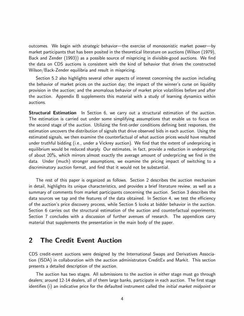
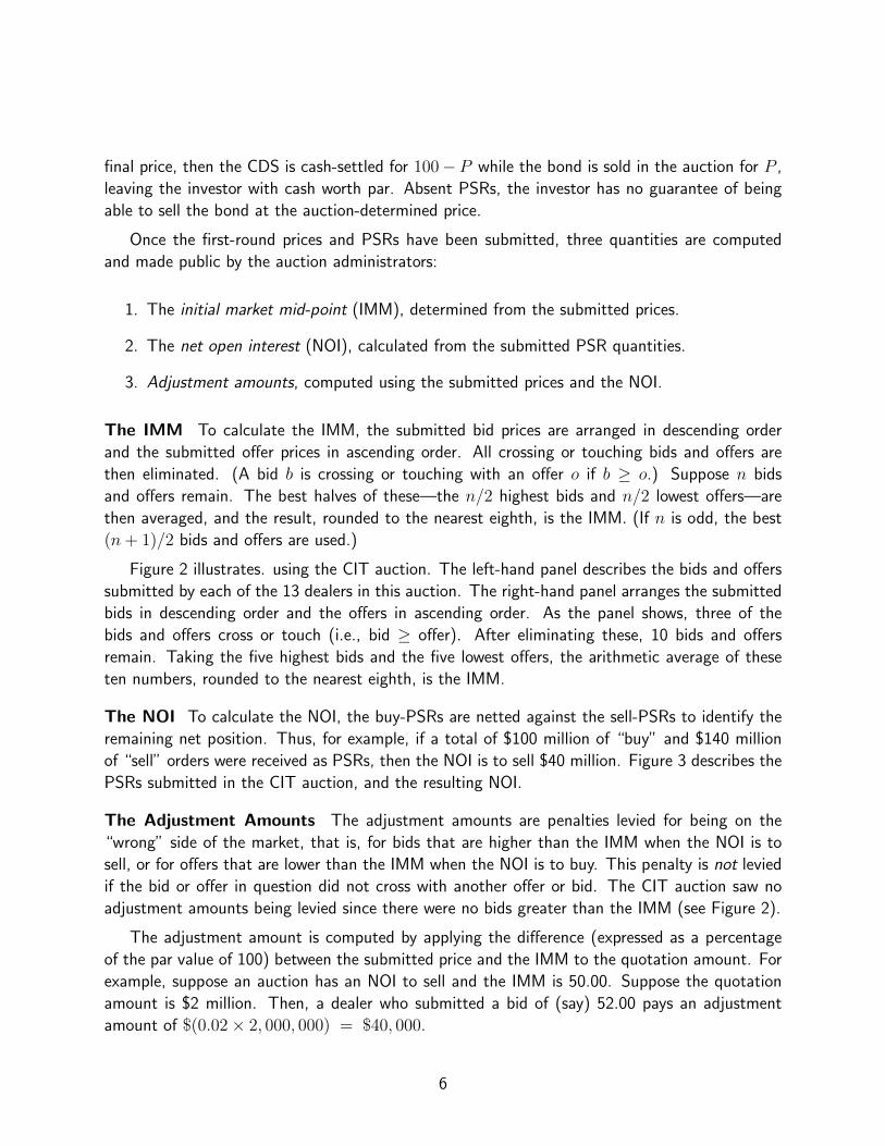
Figure 2 illustrates. using the CIT auction. The left-hand panel describes the bids and offers
submitted by each of the 13 dealers in this auction. The right-hand panel arranges the submitted
bids in descending order and the offers in ascending order. As the panel shows, three of the
bids and offers cross or touch (i.e., bid ≥ offer). After eliminating these, 10 bids and offers
remain. Taking the five highest bids and the five lowest offers, the arithmetic average of these
ten numbers, rounded to the nearest eighth, is the IMM.
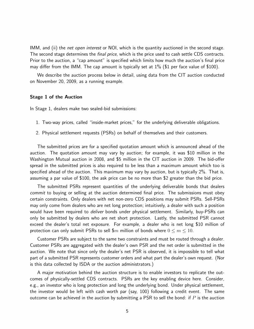
The NOI To calculate the NOI, the buy-PSRs are netted against the sell-PSRs to identify the
remaining net position. Thus, for example, if a total of $100 million of “buy” and $140 million
of “sell” orders were received as PSRs, then the NOI is to sell $40 million. Figure 3 describes the
PSRs submitted in the CIT auction, and the resulting NOI.
The Adjustment Amounts The adjustment amounts are penalties levied for being on the
“wrong” side of the market, that is, for bids that are higher than the IMM when the NOI is to
sell, or for offers that are lower than the IMM when the NOI is to buy. This penalty is not levied
if the bid or offer in question did not cross with another offer or bid. The CIT auction saw no
adjustment amounts being levied since there were no bids greater than the IMM (see Figure 2).
The adjustment amount is computed by applying the difference (expressed as a percentage
of the par value of 100) between the submitted price and the IMM to the quotation amount. For
example, suppose an auction has an NOI to sell and the IMM is 50.00. Suppose the quotation
amount is $2 million. Then, a dealer who submitted a bid of (say) 52.00 pays an adjustment
amount of $(0.02× 2, 000, 000) = $40, 000.
6
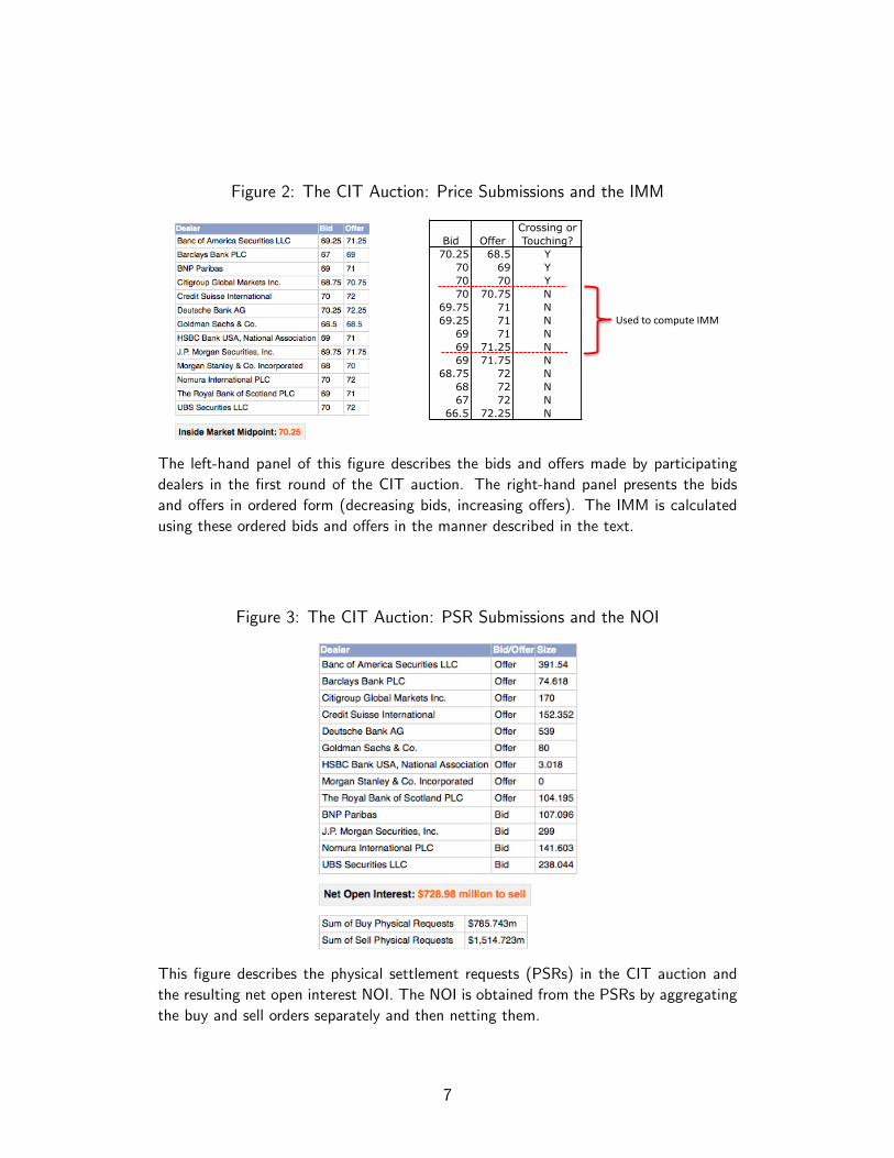
Figure 2: The CIT Auction: Price Submissions and the IMM
Crossing orBid Offer Touching?
70.25 68.5 Y70 69 Y70 70 Y70 70.75 N
69.75 71 N69.25 71 N
69 71 N69 71.25 N69 71.75 N
68.75 72 N68 72 N67 72 N
66.5 72.25 N
Used to compute IMM
The left-hand panel of this figure describes the bids and offers made by participating
dealers in the first round of the CIT auction. The right-hand panel presents the bids
and offers in ordered form (decreasing bids, increasing offers). The IMM is calculated
using these ordered bids and offers in the manner described in the text.
Figure 3: The CIT Auction: PSR Submissions and the NOI
This figure describes the physical settlement requests (PSRs) in the CIT auction and
the resulting net open interest NOI. The NOI is obtained from the PSRs by aggregating
the buy and sell orders separately and then netting them.
7
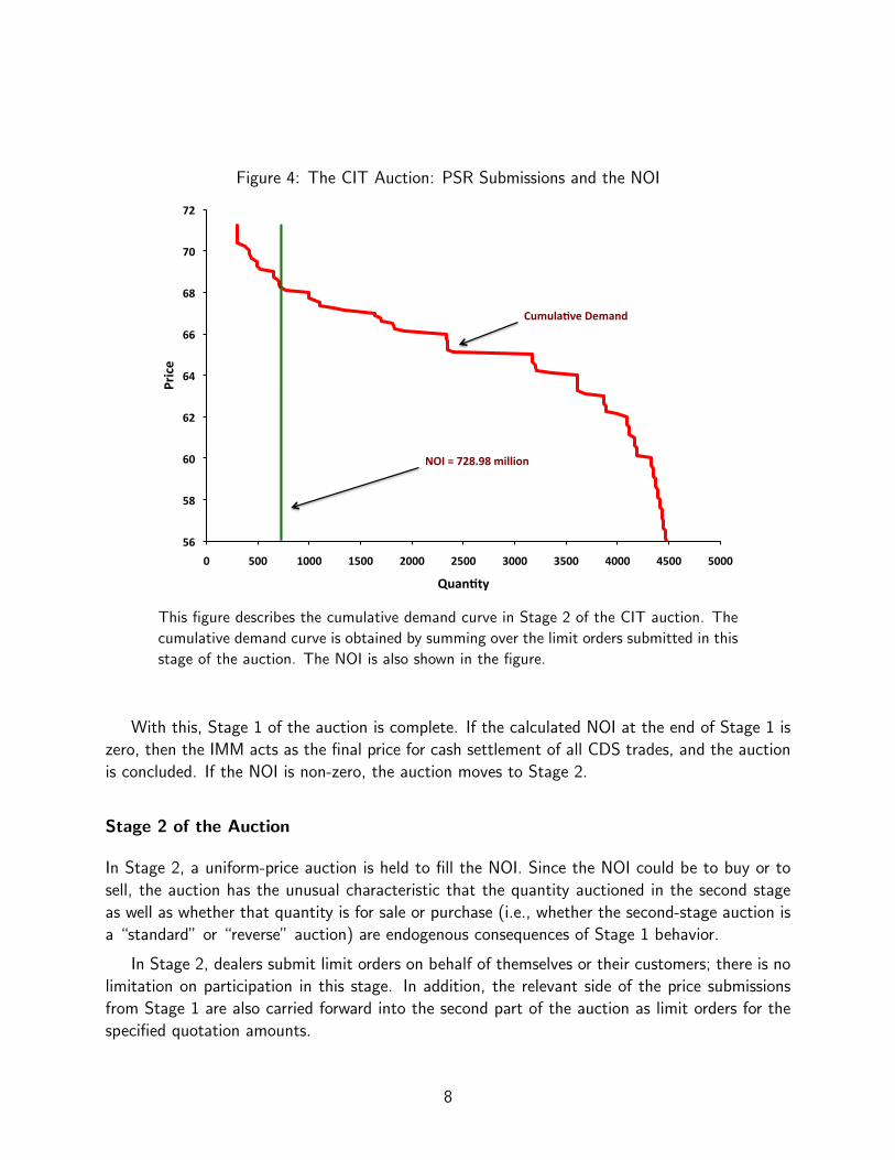
Figure 4: The CIT Auction: PSR Submissions and the NOI
56
58
60
62
64
66
68
70
72
0 500 1000 1500 2000 2500 3000 3500 4000 4500 5000
Price
Quan4ty
NOI = 728.98 million
Cumula4ve Demand
This figure describes the cumulative demand curve in Stage 2 of the CIT auction. The
cumulative demand curve is obtained by summing over the limit orders submitted in this
stage of the auction. The NOI is also shown in the figure.
With this, Stage 1 of the auction is complete. If the calculated NOI at the end of Stage 1 is
zero, then the IMM acts as the final price for cash settlement of all CDS trades, and the auction
is concluded. If the NOI is non-zero, the auction moves to Stage 2.
Stage 2 of the Auction
In Stage 2, a uniform-price auction is held to fill the NOI. Since the NOI could be to buy or to
sell, the auction has the unusual characteristic that the quantity auctioned in the second stage
as well as whether that quantity is for sale or purchase (i.e., whether the second-stage auction is
a “standard” or “reverse” auction) are endogenous consequences of Stage 1 behavior.
In Stage 2, dealers submit limit orders on behalf of themselves or their customers; there is no
limitation on participation in this stage. In addition, the relevant side of the price submissions
from Stage 1 are also carried forward into the second part of the auction as limit orders for the
specified quotation amounts.
8

If sufficient limit order quantities are not received to fill the NOI, then the final price is set
to zero if the NOI is to “sell,” and to par if the NOI is to “buy.” Otherwise, the auction’s final
price is determined from the limit orders as the price that fills the NOI, but with one additional
constraint: If the NOI is to sell, then the final price cannot exceed the IMM plus the cap amount,
while if the NOI is to buy, the final price cannot be less than the IMM minus the cap amount.
Figure 4 shows the cumulative demand curve in the second stage of the CIT auction that
obtains in the obvious way by summing the submitted limit orders. Limit orders were submitted
for prices ranging from 56 to 71.25, and the cumulative quantity demanded, summed over all
prices, was a little under $4.50 billion, over 6 times the NOI of $728.98 million. The final price
in the auction was 68.125.
Relation to Other Auction Forms
The credit-event auction format shares features in common with some other auction forms but
is distinct from all of these, and is more complex than most. In contrast to the endogeneity
of the CDS credit-event auction that was highlighted above, most auctions in practice (and
in the academic literature) deal with a fixed quantity that is specified in advance as being for
sale or purchase. The challenge is to design an auction format that optimizes the auctioneer’s
expected cash flows;5 what makes this a non-trivial problem is asymmetric information, i.e., that
the auctioneer does not know the bidders’ private information concerning the value of the object
being auctioned. There is no analog of this cash flow optimization objective in credit event
auctions; rather, price-discovery and smooth CDS market settlement are the key goals.
Broadly speaking, there are two kinds of auctions to which CDS auctions bear some similar-
ity: two-stage auctions and Treasury auctions. Two-stage auctions, studied in Ye (2007), are
employed to sell complex and high-valued assets. Like CDS auctions, they have a first stage
used to identify an indicative price, and a second round that identifies the definitive final price.
However, the similarities end here. Two-stage auctions are commonly single-unit auctions with
a single winning bidder; there are no first-stage quantity submission decisions to be made by the
participants. More importantly, in two-stage auctions as currently used in practice, the only role
of the first-stage bids is to restrict participation in the second round to those submitting the
highest first-stage bids; the bid has no other payoff consequence.
Auctions of Treasury securities worldwide resemble the second stage of credit-event auctions
with a sell-NOI: in both cases, there is a given quantity being auctioned, bidders submit limit
orders, and the final price is determined by matching the aggregate demand curve to the avail-
able supply. Treasury auctions worldwide have been widely studied in the literature; see, e.g.,
Nyborg and Sundaresan (1996) on US auctions; Nyborg, Rydqvist, and Sundaresan (2002) on
Swedish auctions; Keloharju, Nyborg, and Rydqvist (2005) on Finnish auctions; and Hortacsu or
5That is, maximizes the expected revenues for a “sell” or standard auction, and minimizes expected cashoutflow for a “buy” or reverse auction.
9
MacAdams (2010) on Turkish auctions.
The Literature on Credit-Event Auctions
There are, as far as we know, only four other papers on credit-event auctions. Two of them,
Helwege, et al (2009) and Coudert and Gex (2010) are empirical studies. Helwege, et al, looks
at empirical features of credit-event auctions up to March 2009, including a comparison of the
auction final price to the market prices on the day of and the day after the auction. A portion of
our analysis in Section 4 is based on similar questions, but our analysis has the benefit of more
data and is carried out in greater detail. Coudert and Gex examine the performance of the auction
process in individual cases including Lehman Brothers, Fannie Mae and Freddie Mac. Their focus
is on the functioning of the market in stressful times; they also provide some documentation of
the bounce in prices after the auction date compared to the auction’s final price.
The other two papers, Du and Zhu (2011) and Chernov, Gorbenko, and Makarov (2011)
are primarily theoretical models of CDS auctions. The models are developed in the spirit of
Wilson (1979): there is no asymmetric information, and the post-auction bond value is taken
to be common knowledge. Thus, the typical concerns of the auction literature—price discov-
ery, information generation in the auction, the winner’s curse—are not the focus. Rather, the
question is how strategic behavior could cause the auction-determined price to deviate from this
exogenously-specified “true” price solely on account of monopsonistic behavior.
Taking first stage outcomes as given, Du-Zhu describe a model of the second stage of the
auction. They show that the model has equilibria in which prices are systematically biased,
with sell-auctions resulting in prices that are too high (relative to fair value) and buy-auctions
in prices that are too low. (Taking sell-auctions as the reference point, we will refer to these
as “overpricing” equilibria. As we shall see in Section 4, empirical data exhibits exactly the
opposite pattern to this prediction, namely that of underpricing.) Chernov, Gorbenko and Makarov
derive subgame-perfect equilibria of a full two-stage game. They show that both overpricing and
underpricing equilibria are possible, with the conditions under which the latter obtain depending
on the size of dealers’ net CDS positions entering the second stage relative to the NOI.
3 The Data and Descriptive Statistics
Our auction data comes from http://www.creditfixings.com, a website run by Creditex, one
of the two co-adminstrators of the credit-event auctions. The site provides considerable detail on
each auction including (a) whether auction is an LCDS (Loan CDS) or CDS auction, and in the
latter case, whether the underlying deliverable instruments are senior or subordinated; (b) the list
of deliverable instruments in each auction identified by their ISINs, (c) the list of participating
dealers, (d) the prices and PSRs submitted by each dealer (identified by name) in Stage 1 of
10
the auction, (e) each limit order (price and quantity) submitted by each dealer in Stage 2 of the
auction, (f) whether and what penalties were levied on the dealers, and (g) information on the
auction’s IMM, NOI, and final price.
Table 1 describes the auction types and the names involved in the auctions. There were a
total of 76 auctions over the period 2008-10,6 the bulk of them (51) in 2009. Of these, 54 were
CDS auctions and 22 were LCDS auctions. Our analysis in this paper focuses only on the CDS
auctions. Table 1 provides a list of the underlying firms in these auctions. (Six firm names appear
twice because there were separate auctions for their senior and subordinated bonds.)
Descriptive statistics on deliverable bonds and participation in CDS auctions are presented in
Table 2. Panel A provides summary statistics on the deliverable bonds. On average, there were
30+ deliverable bonds per auction, but with huge variation, ranging from a single deliverable bond
(in 5 different auctions) to a high of 298 deliverables (the CIT auction). The median number
was 5.5, with 6 auctions (all financial firms) having more than 100 deliverable bonds.
Panels B-D of Table 2 deal with dealer participation in the auction. 12-13 dealers participated
in each auction, with the numbers remaining stable over time. Around 75% of all auctions had an
NOI to “sell” at the end of Stage 1, and 25% had an NOI to “buy,” with the split again remaining
roughly stable over time. Dealer participation was roughly the same regardless of whether the
auction turned out to have a buy NOI or a sell NOI, but, as as Panel D shows, the number of limit
orders submitted in the second round was significantly higher for sell-NOI auctions compared to
buy-NOI auctions. The aggregate quantity demanded in Stage 2 (summed over all prices) vastly
exceeded NOI in every auction, although there were often huge bids submitted at very low prices;
Figure 5 illustrates with the Lehman auction: the NOI was $4.92 billion.
Panel C of Table 2 describes the penalties (adjustment amounts) for off-market first-round
price submissions. On average, 1.2 firms got penalized in each auction, with a minimum of zero
and a maximum of 5. Several dealers suffered multiple penalties, with HSBC leading the list with
8 penalties over the three-year span.
Where our analysis only concerns behavior within the auction, we use data from all 48 auctions
involving non-subordinated bonds. Where we also use market prices of the deliverable bonds (e.g.,
in the analysis of price discovery in Section 4), we use market price data from TRACE. We look
mainly at a horizon of 5 trading days before the auction to 5 trading days after the auction.
Market price data is available (i.e., at least one deliverable bond is traded over this horizon) for
27 of the auctions; the names appear in boldface in Panel B of Table 1. The remaining auctions
have deliverables such as trust-issued securities or euro-denominated covered bonds on which
TRACE had no information. Twenty-two of the 27 auctions meet the stronger criterion that
there is at least one trade in a deliverable bond (possibly a different deliverable bond on each
day) on each of the 10 trading days in our horizon; four of these are “buy” auctions (i.e., have a
6There were only three auctions in 2006 and a single one in 2007. Since the format of the auction was changedin late-2006, we focus our analysis on the period 2008-10.
11
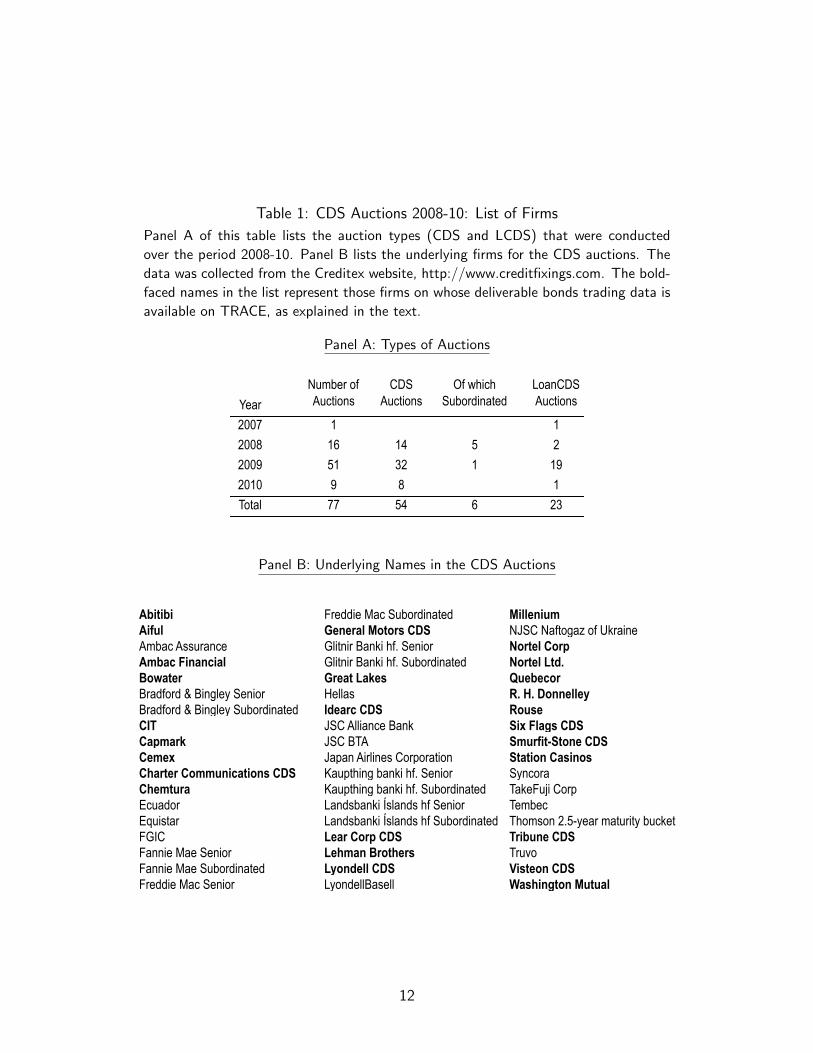
Table 1: CDS Auctions 2008-10: List of Firms
Panel A of this table lists the auction types (CDS and LCDS) that were conducted
over the period 2008-10. Panel B lists the underlying firms for the CDS auctions. The
data was collected from the Creditex website, http://www.creditfixings.com. The bold-
faced names in the list represent those firms on whose deliverable bonds trading data is
available on TRACE, as explained in the text.
Panel A: Types of Auctions
Year
2007 1 1
2008 16 14 5 2
2009 51 32 1 19
2010 9 8 1
Total 77 54 6 23
Number of Auctions
CDS Auctions
LoanCDS Auctions
Of which Subordinated
Panel B: Underlying Names in the CDS Auctions
Abitibi Freddie Mac Subordinated MilleniumAiful General Motors CDS NJSC Naftogaz of UkraineAmbac Assurance Glitnir Banki hf. Senior Nortel CorpAmbac Financial Glitnir Banki hf. Subordinated Nortel Ltd.Bowater Great Lakes QuebecorBradford & Bingley Senior Hellas R. H. DonnelleyBradford & Bingley Subordinated Idearc CDS RouseCIT JSC Alliance Bank Six Flags CDSCapmark JSC BTA Smurfit-Stone CDSCemex Japan Airlines Corporation Station CasinosCharter Communications CDS Kaupthing banki hf. Senior SyncoraChemtura Kaupthing banki hf. Subordinated TakeFuji CorpEcuador Landsbanki Íslands hf Senior TembecEquistar Landsbanki Íslands hf Subordinated Thomson 2.5-year maturity bucketFGIC Lear Corp CDS Tribune CDSFannie Mae Senior Lehman Brothers TruvoFannie Mae Subordinated Lyondell CDS Visteon CDSFreddie Mac Senior LyondellBasell Washington Mutual
12
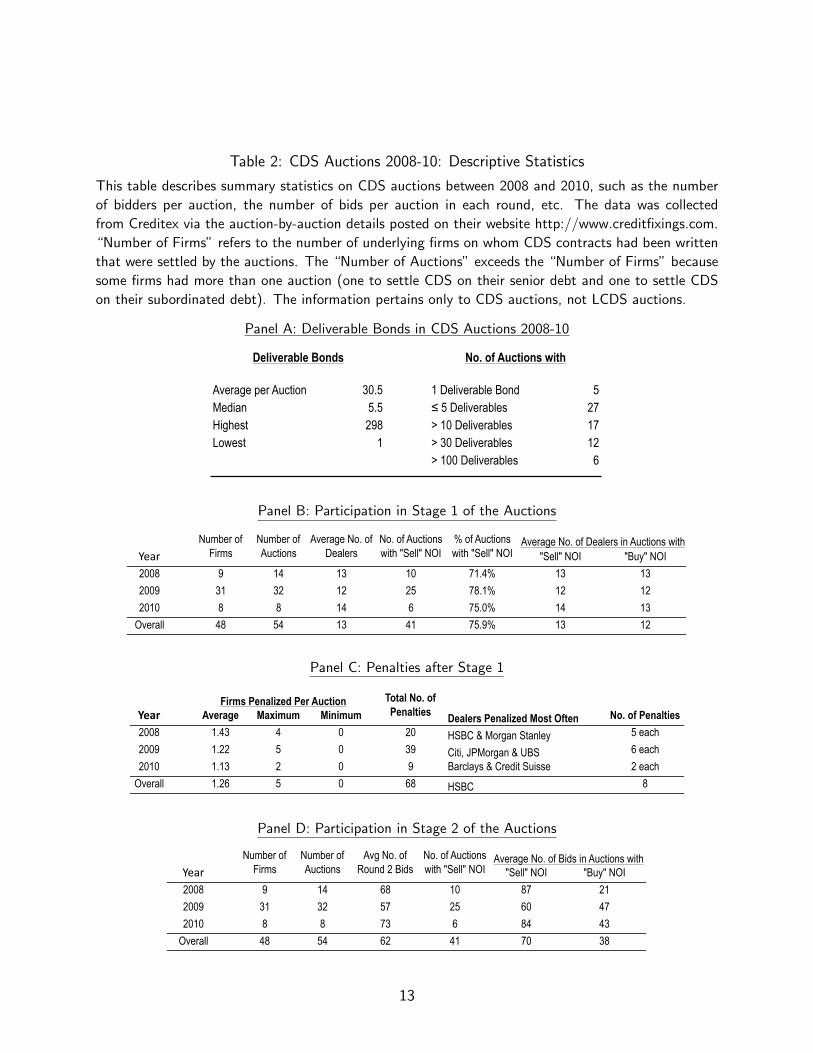
Table 2: CDS Auctions 2008-10: Descriptive Statistics
This table describes summary statistics on CDS auctions between 2008 and 2010, such as the number
of bidders per auction, the number of bids per auction in each round, etc. The data was collected
from Creditex via the auction-by-auction details posted on their website http://www.creditfixings.com.
“Number of Firms” refers to the number of underlying firms on whom CDS contracts had been written
that were settled by the auctions. The “Number of Auctions” exceeds the “Number of Firms” because
some firms had more than one auction (one to settle CDS on their senior debt and one to settle CDS
on their subordinated debt). The information pertains only to CDS auctions, not LCDS auctions.
Panel A: Deliverable Bonds in CDS Auctions 2008-10
Average per Auction 30.5 1 Deliverable Bond 5Median 5.5 ≤ 5 Deliverables 27Highest 298 > 10 Deliverables 17Lowest 1 > 30 Deliverables 12
> 100 Deliverables 6
Deliverable Bonds No. of Auctions with
Panel B: Participation in Stage 1 of the Auctions
Year "Sell" NOI "Buy" NOI
2008 9 14 13 10 71.4% 13 13
2009 31 32 12 25 78.1% 12 12
2010 8 8 14 6 75.0% 14 13
Overall 48 54 13 41 75.9% 13 12
Participation in Round 1 of the AuctionsNumber of
FirmsNumber of Auctions
Average No. of Dealers
No. of Auctions with "Sell" NOI
% of Auctions with "Sell" NOI
Average No. of Dealers in Auctions with
Panel C: Penalties after Stage 1
Year Average Maximum Minimum No. of Penalties
2008 1.43 4 0 20 5 each
2009 1.22 5 0 39 6 each
2010 1.13 2 0 9 Barclays & Credit Suisse 2 each
Overall 1.26 5 0 68 8HSBC
Firms Penalized Per Auction Total No. of Penalties Dealers Penalized Most Often
HSBC & Morgan Stanley
Citi, JPMorgan & UBS
Panel D: Participation in Stage 2 of the Auctions
Year "Sell" NOI "Buy" NOI
2008 9 14 68 10 87 21
2009 31 32 57 25 60 47
2010 8 8 73 6 84 43
Overall 48 54 62 41 70 38
Participation in Round 2: Bids/OffersNumber of
FirmsNumber of Auctions
Avg No. of Round 2 Bids
No. of Auctions with "Sell" NOI
Average No. of Bids in Auctions with
13
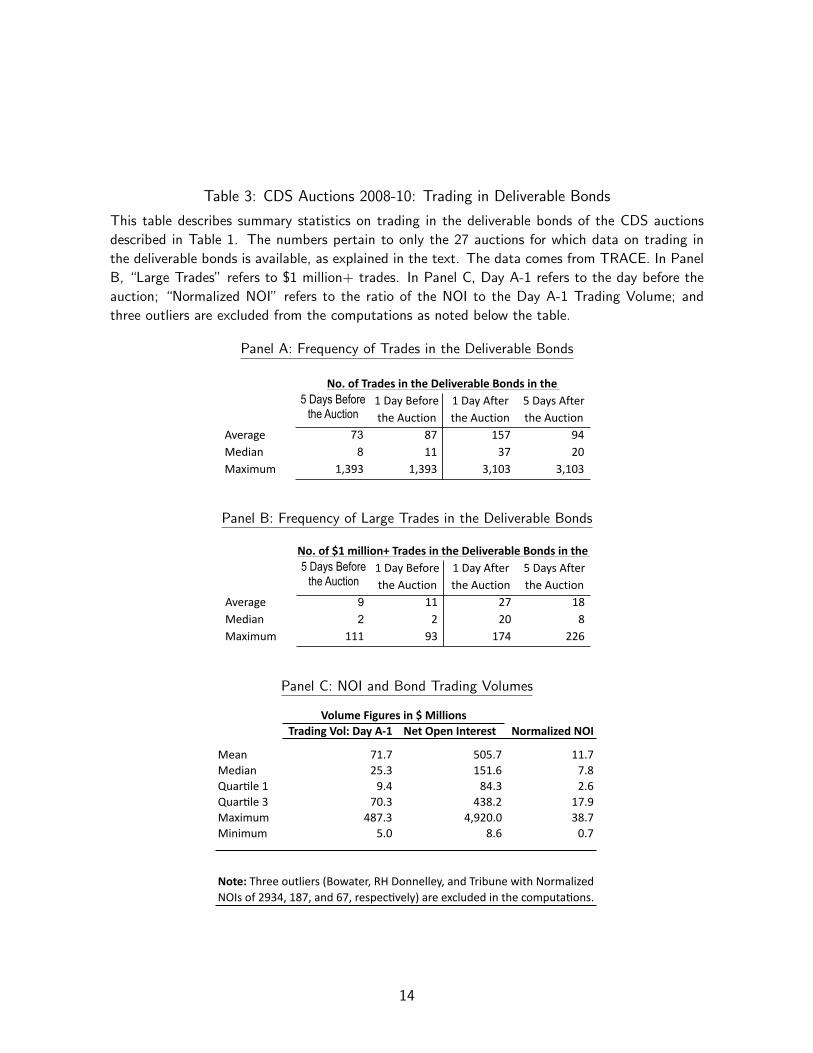
Table 3: CDS Auctions 2008-10: Trading in Deliverable Bonds
This table describes summary statistics on trading in the deliverable bonds of the CDS auctions
described in Table 1. The numbers pertain to only the 27 auctions for which data on trading in
the deliverable bonds is available, as explained in the text. The data comes from TRACE. In Panel
B, “Large Trades” refers to $1 million+ trades. In Panel C, Day A-1 refers to the day before the
auction; “Normalized NOI” refers to the ratio of the NOI to the Day A-1 Trading Volume; and
three outliers are excluded from the computations as noted below the table.
Panel A: Frequency of Trades in the Deliverable Bonds
Average 73 87 157 94Median 8 11 37 20Maximum 1,393 1,393 3,103 3,103
No.ofTradesintheDeliverableBondsinthe5 Days Before
the Auction1DayBeforetheAuction
1DayAftertheAuction
5DaysAftertheAuction
Panel B: Frequency of Large Trades in the Deliverable Bonds
Average 9 11 27 18Median 2 2 20 8Maximum 111 93 174 226
No.of$1million+TradesintheDeliverableBondsinthe5 Days Before
the Auction1DayBeforetheAuction
1DayAftertheAuction
5DaysAftertheAuction
Panel C: NOI and Bond Trading Volumes
Trading Vol: Day A-‐1 Net Open Interest Normalized NOI
Mean 71.7 505.7 11.7Median 25.3 151.6 7.8Quar3le 1 9.4 84.3 2.6Quar3le 3 70.3 438.2 17.9Maximum 487.3 4,920.0 38.7Minimum 5.0 8.6 0.7
Note: Three outliers (Bowater, RH Donnelley, and Tribune with Normalized NOIs of 2934, 187, and 67, respec3vely) are excluded in the computa3ons.
Volume Figures in $ Millions
14
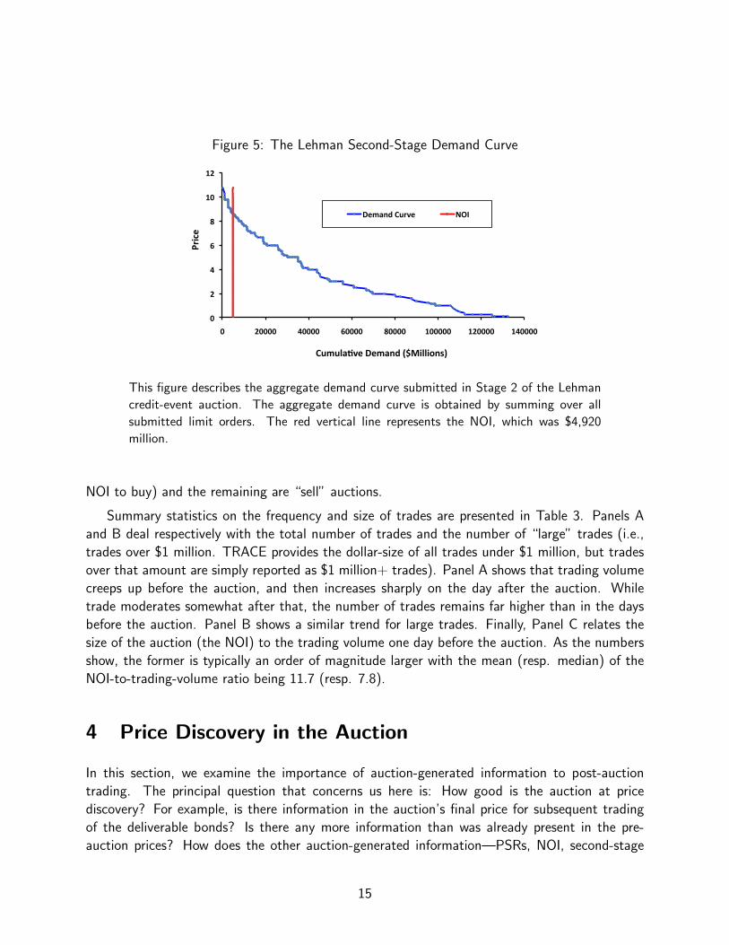
Figure 5: The Lehman Second-Stage Demand Curve
0
2
4
6
8
10
12
0 20000 40000 60000 80000 100000 120000 140000
Price
Cumula2ve Demand ($Millions)
Lehman Round 2 Demand Curve
Demand Curve NOI
This figure describes the aggregate demand curve submitted in Stage 2 of the Lehman
credit-event auction. The aggregate demand curve is obtained by summing over all
submitted limit orders. The red vertical line represents the NOI, which was $4,920
million.
NOI to buy) and the remaining are “sell” auctions.
Summary statistics on the frequency and size of trades are presented in Table 3. Panels A
and B deal respectively with the total number of trades and the number of “large” trades (i.e.,
trades over $1 million. TRACE provides the dollar-size of all trades under $1 million, but trades
over that amount are simply reported as $1 million+ trades). Panel A shows that trading volume
creeps up before the auction, and then increases sharply on the day after the auction. While
trade moderates somewhat after that, the number of trades remains far higher than in the days
before the auction. Panel B shows a similar trend for large trades. Finally, Panel C relates the
size of the auction (the NOI) to the trading volume one day before the auction. As the numbers
show, the former is typically an order of magnitude larger with the mean (resp. median) of the
NOI-to-trading-volume ratio being 11.7 (resp. 7.8).
4 Price Discovery in the Auction
In this section, we examine the importance of auction-generated information to post-auction
trading. The principal question that concerns us here is: How good is the auction at price
discovery? For example, is there information in the auction’s final price for subsequent trading
of the deliverable bonds? Is there any more information than was already present in the pre-
auction prices? How does the other auction-generated information—PSRs, NOI, second-stage
15
limit orders—affect post-auction behavior? We use data on market prices and traded quantities
for the deliverable bonds in the 27 boldfaced auctions of Table 1 to study these questions.
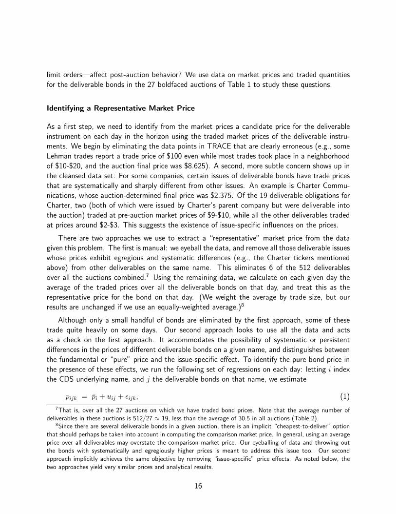
Identifying a Representative Market Price
As a first step, we need to identify from the market prices a candidate price for the deliverable
instrument on each day in the horizon using the traded market prices of the deliverable instru-
ments. We begin by eliminating the data points in TRACE that are clearly erroneous (e.g., some
Lehman trades report a trade price of $100 even while most trades took place in a neighborhood
of $10-$20, and the auction final price was $8.625). A second, more subtle concern shows up in
the cleansed data set: For some companies, certain issues of deliverable bonds have trade prices
that are systematically and sharply different from other issues. An example is Charter Commu-
nications, whose auction-determined final price was $2.375. Of the 19 deliverable obligations for
Charter, two (both of which were issued by Charter’s parent company but were deliverable into
the auction) traded at pre-auction market prices of $9-$10, while all the other deliverables traded
at prices around $2-$3. This suggests the existence of issue-specific influences on the prices.
There are two approaches we use to extract a “representative” market price from the data
given this problem. The first is manual: we eyeball the data, and remove all those deliverable issues
whose prices exhibit egregious and systematic differences (e.g., the Charter tickers mentioned
above) from other deliverables on the same name. This eliminates 6 of the 512 deliverables
over all the auctions combined.7 Using the remaining data, we calculate on each given day the
average of the traded prices over all the deliverable bonds on that day, and treat this as the
representative price for the bond on that day. (We weight the average by trade size, but our
results are unchanged if we use an equally-weighted average.)8
Although only a small handful of bonds are eliminated by the first approach, some of these
trade quite heavily on some days. Our second approach looks to use all the data and acts
as a check on the first approach. It accommodates the possibility of systematic or persistent
differences in the prices of different deliverable bonds on a given name, and distinguishes between
the fundamental or “pure” price and the issue-specific effect. To identify the pure bond price in
the presence of these effects, we run the following set of regressions on each day: letting i index
the CDS underlying name, and j the deliverable bonds on that name, we estimate
pijk = p̄i + uij + εijk, (1)
7That is, over all the 27 auctions on which we have traded bond prices. Note that the average number ofdeliverables in these auctions is 512/27 ≈ 19, less than the average of 30.5 in all auctions (Table 2).
8Since there are several deliverable bonds in a given auction, there is an implicit “cheapest-to-deliver” optionthat should perhaps be taken into account in computing the comparison market price. In general, using an averageprice over all deliverables may overstate the comparison market price. Our eyeballing of data and throwing outthe bonds with systematically and egregiously higher prices is meant to address this issue too. Our secondapproach implicitly achieves the same objective by removing “issue-specific” price effects. As noted below, thetwo approaches yield very similar prices and analytical results.
16
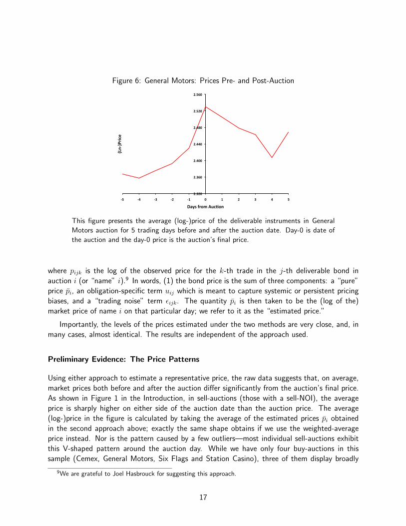
Figure 6: General Motors: Prices Pre- and Post-Auction
2.320
2.360
2.400
2.440
2.480
2.520
2.560
-‐5 -‐4 -‐3 -‐2 -‐1 0 1 2 3 4 5
(Ln-‐)Price
Days from Auc>on
This figure presents the average (log-)price of the deliverable instruments in General
Motors auction for 5 trading days before and after the auction date. Day-0 is date of
the auction and the day-0 price is the auction’s final price.
where pijk is the log of the observed price for the k-th trade in the j-th deliverable bond in
auction i (or “name” i).9 In words, (1) the bond price is the sum of three components: a “pure”
price p̄i, an obligation-specific term uij which is meant to capture systemic or persistent pricing
biases, and a “trading noise” term εijk. The quantity p̄i is then taken to be the (log of the)
market price of name i on that particular day; we refer to it as the “estimated price.”
Importantly, the levels of the prices estimated under the two methods are very close, and, in
many cases, almost identical. The results are independent of the approach used.
Preliminary Evidence: The Price Patterns
Using either approach to estimate a representative price, the raw data suggests that, on average,
market prices both before and after the auction differ significantly from the auction’s final price.
As shown in Figure 1 in the Introduction, in sell-auctions (those with a sell-NOI), the average
price is sharply higher on either side of the auction date than the auction price. The average
(log-)price in the figure is calculated by taking the average of the estimated prices p̄i obtained
in the second approach above; exactly the same shape obtains if we use the weighted-average
price instead. Nor is the pattern caused by a few outliers—most individual sell-auctions exhibit
this V-shaped pattern around the auction day. While we have only four buy-auctions in this
sample (Cemex, General Motors, Six Flags and Station Casino), three of them display broadly
9We are grateful to Joel Hasbrouck for suggesting this approach.
17
the opposite pattern; Figure 6 describes the behavior of General Motors’ prices.
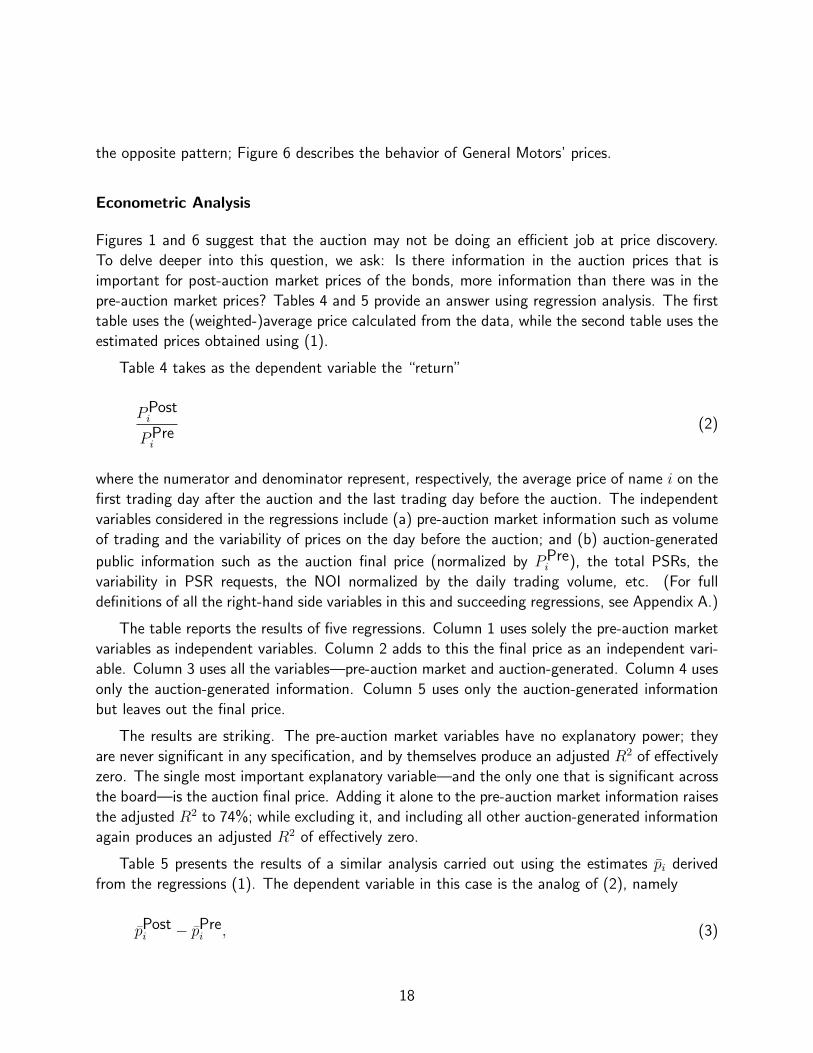
Econometric Analysis
Figures 1 and 6 suggest that the auction may not be doing an efficient job at price discovery.
To delve deeper into this question, we ask: Is there information in the auction prices that is
important for post-auction market prices of the bonds, more information than there was in the
pre-auction market prices? Tables 4 and 5 provide an answer using regression analysis. The first
table uses the (weighted-)average price calculated from the data, while the second table uses the
estimated prices obtained using (1).
Table 4 takes as the dependent variable the “return”
PPosti
PPrei
(2)
where the numerator and denominator represent, respectively, the average price of name i on the
first trading day after the auction and the last trading day before the auction. The independent
variables considered in the regressions include (a) pre-auction market information such as volume
of trading and the variability of prices on the day before the auction; and (b) auction-generated
public information such as the auction final price (normalized by PPrei ), the total PSRs, the
variability in PSR requests, the NOI normalized by the daily trading volume, etc. (For full
definitions of all the right-hand side variables in this and succeeding regressions, see Appendix A.)
The table reports the results of five regressions. Column 1 uses solely the pre-auction market
variables as independent variables. Column 2 adds to this the final price as an independent vari-
able. Column 3 uses all the variables—pre-auction market and auction-generated. Column 4 uses
only the auction-generated information. Column 5 uses only the auction-generated information
but leaves out the final price.
The results are striking. The pre-auction market variables have no explanatory power; they
are never significant in any specification, and by themselves produce an adjusted R2 of effectively
zero. The single most important explanatory variable—and the only one that is significant across
the board—is the auction final price. Adding it alone to the pre-auction market information raises
the adjusted R2 to 74%; while excluding it, and including all other auction-generated information
again produces an adjusted R2 of effectively zero.
Table 5 presents the results of a similar analysis carried out using the estimates p̄i derived
from the regressions (1). The dependent variable in this case is the analog of (2), namely
p̄Posti − p̄Pre
i , (3)
18
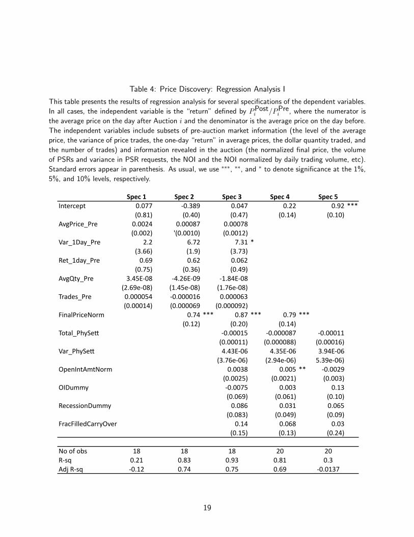
Table 4: Price Discovery: Regression Analysis I
This table presents the results of regression analysis for several specifications of the dependent variables.
In all cases, the independent variable is the “return” defined by PPosti /PPre
i , where the numerator is
the average price on the day after Auction i and the denominator is the average price on the day before.
The independent variables include subsets of pre-auction market information (the level of the average
price, the variance of price trades, the one-day “return” in average prices, the dollar quantity traded, and
the number of trades) and information revealed in the auction (the normalized final price, the volume
of PSRs and variance in PSR requests, the NOI and the NOI normalized by daily trading volume, etc).
Standard errors appear in parenthesis. As usual, we use ∗∗∗, ∗∗, and ∗ to denote significance at the 1%,
5%, and 10% levels, respectively.
Spec 1 Spec 2 Spec 3 Spec 4 Spec 5Intercept 0.077 -‐0.389 0.047 0.22 0.92 ***
(0.81) (0.40) (0.47) (0.14) (0.10)AvgPrice_Pre 0.0024 0.00087 0.00078
(0.002) '(0.0010) (0.0012)Var_1Day_Pre 2.2 6.72 7.31 *
(3.66) (1.9) (3.73)Ret_1day_Pre 0.69 0.62 0.062
(0.75) (0.36) (0.49)AvgQty_Pre 3.45E-‐08 -‐4.26E-‐09 -‐1.84E-‐08
(2.69e-‐08) (1.45e-‐08) (1.76e-‐08)Trades_Pre 0.000054 -‐0.000016 0.000063
(0.00014) (0.000069 (0.000092)FinalPriceNorm 0.74 *** 0.87 *** 0.79 ***
(0.12) (0.20) (0.14)Total_PhySeO -‐0.00015 -‐0.000087 -‐0.00011
(0.00011) (0.000088) (0.00016)Var_PhySeO 4.43E-‐06 4.35E-‐06 3.94E-‐06
(3.76e-‐06) (2.94e-‐06) 5.39e-‐06)OpenIntAmtNorm 0.0038 0.005 ** -‐0.0029
(0.0025) (0.0021) (0.003)OIDummy -‐0.0075 0.003 0.13
(0.069) (0.061) (0.10)RecessionDummy 0.086 0.031 0.065
(0.083) (0.049) (0.09)FracFilledCarryOver 0.14 0.068 0.03
(0.15) (0.13) (0.24)
No of obs 18 18 18 20 20R-‐sq 0.21 0.83 0.93 0.81 0.3Adj R-‐sq -‐0.12 0.74 0.75 0.69 -‐0.0137
19
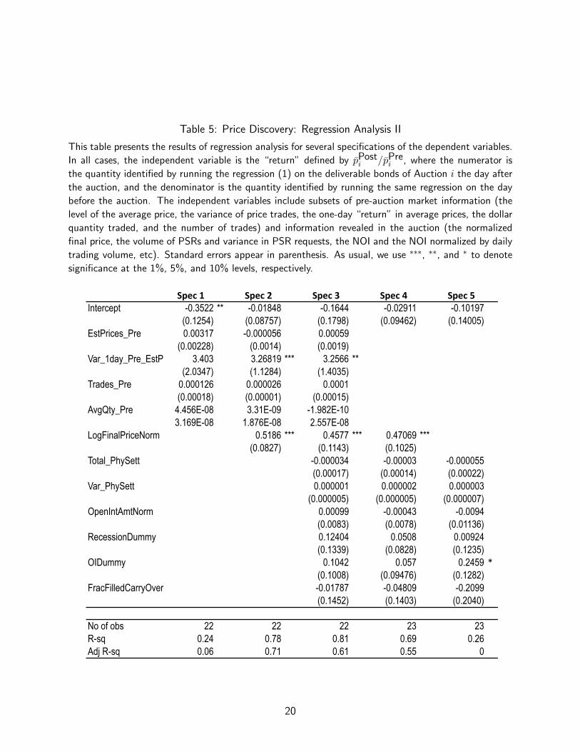
Table 5: Price Discovery: Regression Analysis II
This table presents the results of regression analysis for several specifications of the dependent variables.
In all cases, the independent variable is the “return” defined by p̄Posti /p̄Pre
i , where the numerator is
the quantity identified by running the regression (1) on the deliverable bonds of Auction i the day after
the auction, and the denominator is the quantity identified by running the same regression on the day
before the auction. The independent variables include subsets of pre-auction market information (the
level of the average price, the variance of price trades, the one-day “return” in average prices, the dollar
quantity traded, and the number of trades) and information revealed in the auction (the normalized
final price, the volume of PSRs and variance in PSR requests, the NOI and the NOI normalized by daily
trading volume, etc). Standard errors appear in parenthesis. As usual, we use ∗∗∗, ∗∗, and ∗ to denote
significance at the 1%, 5%, and 10% levels, respectively.
Spec 1 Spec 2 Spec 3 Spec 4 Spec 5Intercept -0.3522 ** -0.01848 -0.1644 -0.02911 -0.10197
(0.1254) (0.08757) (0.1798) (0.09462) (0.14005)EstPrices_Pre 0.00317 -0.000056 0.00059
(0.00228) (0.0014) (0.0019)Var_1day_Pre_EstP 3.403 3.26819 *** 3.2566 **
(2.0347) (1.1284) (1.4035)Trades_Pre 0.000126 0.000026 0.0001
(0.00018) (0.00001) (0.00015)AvgQty_Pre 4.456E-08 3.31E-09 -1.982E-10
3.169E-08 1.876E-08 2.557E-08LogFinalPriceNorm 0.5186 *** 0.4577 *** 0.47069 ***
(0.0827) (0.1143) (0.1025)Total_PhySett -0.000034 -0.00003 -0.000055
(0.00017) (0.00014) (0.00022)Var_PhySett 0.000001 0.000002 0.000003
(0.000005) (0.000005) (0.000007)OpenIntAmtNorm 0.00099 -0.00043 -0.0094
(0.0083) (0.0078) (0.01136)RecessionDummy 0.12404 0.0508 0.00924
(0.1339) (0.0828) (0.1235)OIDummy 0.1042 0.057 0.2459 *
(0.1008) (0.09476) (0.1282)FracFilledCarryOver -0.01787 -0.04809 -0.2099
(0.1452) (0.1403) (0.2040)
No of obs 22 22 22 23 23R-sq 0.24 0.78 0.81 0.69 0.26Adj R-sq 0.06 0.71 0.61 0.55 0
20
where p̄Posti and p̄Pre
i are the estimates of p̄i derived one day after and one day before the
auction, respectively. The right-hand side variables again include several pre-auction market price
and quantity variables, and auction-generated information. The key component of the latter, the
analog of the normalized final price in the first regression, is the quantity
ln(PAuci )− p̄Pre
i , (4)
where PAuci is just the final price determined in auction i.
Once again, the results are striking, and strongly back the findings in Table 4 on the relevance
especially of the auction-generated final price. When no auction-generated information is included
in the regression (Column 1), the regression has no explanatory power; none of the pre-auction
variables are significant and the adjusted R2 is a bit under 6%. Adding the normalized final price
(4) alone to the right-hand side variables increases the adjusted R2 to 71%, with the newly added
variable being highly significant. The normalized final price is, indeed, the only variable to be
significant across the board, and in the presence of both market and auction-generated variables.
In summary, the evidence is strong that auction prices are biased but informative. What then
could be the source of the observed biases? We turn to an examination of this question.
5 Behavior in the Auction
An immediate suspect for the observed underpricing is, as noted in the Introduction, the presence
of a “winner’s curse” effect, which should cause participants to bid more conservatively. In
Section 5.1, we gauge the impact of the winner’s curse on bidding behavior and auction outcomes.
Section 5.2 then turns to an examination of other aspects of bidding behavior. We begin with
the effect of a second factor that the theoretical literature has suggested could potentially lead
to underpricing: strategic behavior by participants, i.e., the exercise of market power. Then, we
highlight a number of other interesting aspects of the auction including including the impact of
the winner’s curse on liquidity provision in the auction; the behavior of market price volatilities
pre- and post-auction; and the behavior of market prices on the day of auction. Appendix B
supplements this presentation with a study of the learning dynamics within auctions.
5.1 The Winner’s Curse, Bid Shading, and Auction Underpricing
The winner’s curse is a function of how dispersed is the information entering the auction. We
proxy its intensity using the variance of the first-round price submissions made by dealers. The
justification is obvious: to the extent that these submissions are based on a dealer’s informa-
tion concerning the fair price of the good being auctioned, a more disperse set of first-round
submissions implies a more dispersed information set, and so a more severe winner’s curse.
21
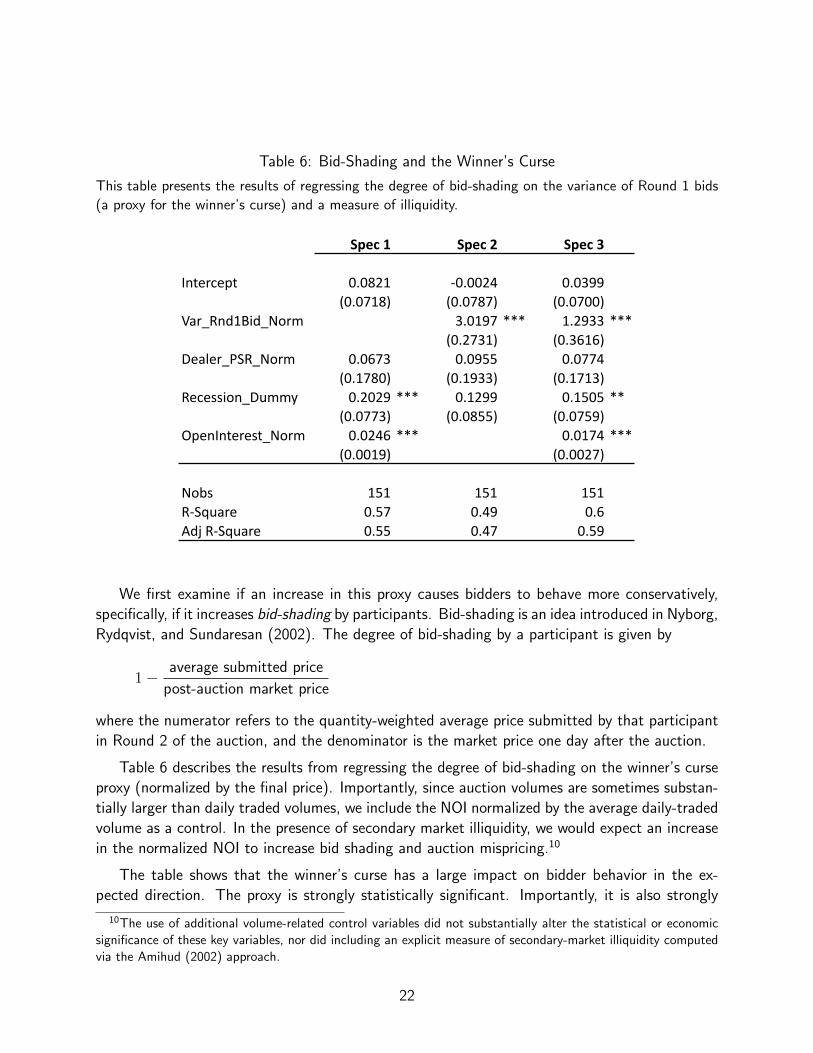
Table 6: Bid-Shading and the Winner’s Curse
This table presents the results of regressing the degree of bid-shading on the variance of Round 1 bids
(a proxy for the winner’s curse) and a measure of illiquidity.
Spec 1 Spec 2 Spec 3
Intercept 0.0821 -‐0.0024 0.0399(0.0718) (0.0787) (0.0700)
Var_Rnd1Bid_Norm 3.0197 *** 1.2933 ***(0.2731) (0.3616)
Dealer_PSR_Norm 0.0673 0.0955 0.0774(0.1780) (0.1933) (0.1713)
Recession_Dummy 0.2029 *** 0.1299 0.1505 **(0.0773) (0.0855) (0.0759)
OpenInterest_Norm 0.0246 *** 0.0174 ***(0.0019) (0.0027)
Nobs 151 151 151R-‐Square 0.57 0.49 0.6Adj R-‐Square 0.55 0.47 0.59
We first examine if an increase in this proxy causes bidders to behave more conservatively,
specifically, if it increases bid-shading by participants. Bid-shading is an idea introduced in Nyborg,
Rydqvist, and Sundaresan (2002). The degree of bid-shading by a participant is given by
1− average submitted price
post-auction market price
where the numerator refers to the quantity-weighted average price submitted by that participant
in Round 2 of the auction, and the denominator is the market price one day after the auction.
Table 6 describes the results from regressing the degree of bid-shading on the winner’s curse
proxy (normalized by the final price). Importantly, since auction volumes are sometimes substan-
tially larger than daily traded volumes, we include the NOI normalized by the average daily-traded
volume as a control. In the presence of secondary market illiquidity, we would expect an increase
in the normalized NOI to increase bid shading and auction mispricing.10
The table shows that the winner’s curse has a large impact on bidder behavior in the ex-
pected direction. The proxy is strongly statistically significant. Importantly, it is also strongly
10The use of additional volume-related control variables did not substantially alter the statistical or economicsignificance of these key variables, nor did including an explicit measure of secondary-market illiquidity computedvia the Amihud (2002) approach.
22
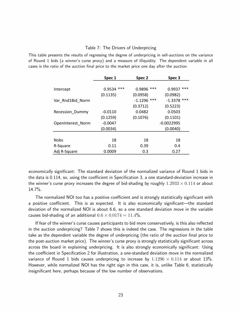
Table 7: The Drivers of Underpricing
This table presents the results of regressing the degree of underpricing in sell-auctions on the variance
of Round 1 bids (a winner’s curse proxy) and a measure of illiquidity. The dependent variable in all
cases is the ratio of the auction final price to the market price one day after the auction.
Spec 1 Spec 2 Spec 3
Intercept 0.9534 *** 0.9896 *** 0.9937 ***(0.1135) (0.0958) (0.0982)
Var_Rnd1Bid_Norm -‐1.1296 *** -‐1.3378 ***(0.3712) (0.5223)
Recession_Dummy -‐0.0110 0.0482 0.0503(0.1259) (0.1076) (0.1101)
OpenInterest_Norm -‐0.0047 -‐0.0022995(0.0034) (0.0040)
Nobs 18 18 18R-‐Square 0.11 0.39 0.4Adj R-‐Square 0.0009 0.3 0.27
economically significant: The standard deviation of the normalized variance of Round 1 bids in
the data is 0.114, so, using the coefficient in Specification 3, a one standard-deviation increase in
the winner’s curse proxy increases the degree of bid-shading by roughly 1.2933× 0.114 or about
14.7%.
The normalized NOI too has a positive coefficient and is strongly statistically significant with
a positive coefficient. This is as expected. It is also economically significant—the standard
deviation of the normalized NOI is about 6.6, so a one standard deviation move in the variable
causes bid-shading of an additional 6.6× 0.0174 = 11.4%.
If fear of the winner’s curse causes participants to bid more conservatively, is this also reflected
in the auction underpricing? Table 7 shows this is indeed the case. The regressions in the table
take as the dependent variable the degree of underpricing (the ratio of the auction final price to
the post-auction market price). The winner’s curse proxy is strongly statistically significant across
across the board in explaining underpricing. It is also strongly economically significant: Using
the coefficient in Specification 2 for illustration, a one-standard deviation move in the normalized
variance of Round 1 bids causes underpricing to increase by 1.1296 × 0.114 or about 13%.
However, while normalized NOI has the right sign in this case, it is, unlike Table 6, statistically
insignificant here, perhaps because of the low number of observations.
23

Table 8: The Impact of Strategic Considerations
This table presents the results of a two-stage estimation of the effect of the slope of the aggregate
demand curve facing a dealer (i.e., the slope of the sum of all the other dealers’ demand curves) on
the slope of responding dealer’s submitted demand curve. In the first stage of the estimation process,
we instrument the slope of the aggregate demand curve, and in the second stage estimate the desired
impact. Further details may be found in the text.
Intercept -‐2.2417 ** Intercept 7.2844 ***(1.0232) (2.2608)
Var_CompPhysSe@ 8.95E-‐06 *** Avg_CompSlope 1.8586 **(2.97E-‐06) (0.8580)
Var_Rnd1Bid 0.9997 Var_Rnd1Bid -‐16.6123 ***(0.727) (4.6125)
OpenInt_Norm -‐0.0500 OpenInt_Norm 0.0645(0.0862) (0.2401)
Var_1DayPre -‐1.0382 ***(0.3965) No of Obs 92
R-‐sq 10.27No of Obs 92R-‐sq 26.25 Test of Endogeneity Adj R-‐sq 22.85F 4.04Prob > F 0.005 (p = 0.0815)
First StageDependent Variable: Avg_CompSlope
Ho: variables are exogenousGMM C Sta^s^c chi^2(1): 3.0354
Second StateDependent Variable: DealerSlope
24
5.2 Other Aspects of Auction Behavior
This section examines several other aspects of auction outcomes. We begin with a look at the
impact of strategic behavior on auction outcomes. Then, we move on to an examination of
liquidity provision in the auction and the role played by the winner’s curse here. Thirdly, we look
at the behavior of market volatilities pre- and post-auction, and highlight an apparent puzzle.
Finally, we examine the behavior of market prices on the auction day. Appendix B supplements
this material by pointing to some interesting aspects of within-auction learning dynamics.
Liquidity and Strategic Considerations
Wilson (1979) and Back and Zender (1993) suggest that “strategic” behavior by bidders (the
exercise of monopsonistic market power) may result in underpricing in divisible-good auctions.
A fundamental insight in their approach is that the marginal cost curve facing a bidder in a
uniform-price auction is endogenous; it is determined by the residual supply curve after subtract-
ing the total demand curve of the other bidders. Using this insight, Wilson and Back-Zender
construct equilibria in their respective models in which the submission of steep demand curves
by the remaining bidders leads the last bidder to respond also with a steep demand curve. The
consequence is underpricing in equilibrium.11
Motivated by the Wilson/Back-Zender arguments, we examine how the slope of the submitted
demand curve for one dealer reacts to an increase in the slopes of the others’ aggregate curve.
Since the slopes are jointly determined in equilibrium, there is an endogeneity problem that must
be addressed. We apply a two-stage estimation process where in the first stage we estimate the
average of the competitors’ slopes as a function of the variance of Round 1 price submissions
and the variance of the competitors’ physical settlement requests. The first of these variables is
included to control for asymmetric information. The second variable, the variance of competitors’
PSRs, is an instrument for the average competitors’ slope. The choice of instrument need meet
two conditions: that it affect the competitor’s slope and that it not affect the dealer’s own
slope. PSRs, which represent customer orders, provide dealers with information, so affect their
aggressiveness and the slope of the submitted demand curve. The variance of the competitors’
PSRs is based on each competitor’s PSR and hence should affect the competitor’s slopes. However
it should not affect the dealer’s own slope.
Table 8 presents the findings. In line with the Wilson/Back-Zender hypothesis, the coefficients
of the second-stage regression show that an increase in the competitor’s average slope leads to
a sharp increase in the dealer’s own submitted slope. The choice of instrument is also backed
(albeit, with a p-value of 0.08, somewhat weakly).
11The Wilson/Back-Zender models have no asymmetric information, so the “true” price of the good beingauctioned is common knowledge. “Underpricing” means that the equilibrium price is lower than this true price.
25
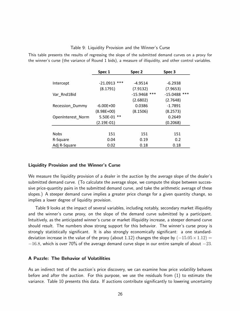
Table 9: Liquidity Provision and the Winner’s Curse
This table presents the results of regressing the slope of the submitted demand curves on a proxy for
the winner’s curse (the variance of Round 1 bids), a measure of illiquidity, and other control variables.
Spec 1 Spec 2 Spec 3
Intercept -‐21.0913 *** -‐4.9514 -‐6.2938(8.1791) (7.9132) (7.9653)
Var_Rnd1Bid -‐15.9468 *** -‐15.0488 ***(2.6802) (2.7648)
Recession_Dummy -‐6.00E+00 0.0386 -‐1.7891(8.98E+00) (8.1506) (8.2573)
OpenInterest_Norm 5.50E-‐01 ** 0.2649(2.19E-‐01) (0.2068)
Nobs 151 151 151R-‐Square 0.04 0.19 0.2Adj R-‐Square 0.02 0.18 0.18
Liquidity Provision and the Winner’s Curse
We measure the liquidity provision of a dealer in the auction by the average slope of the dealer’s
submitted demand curve. (To calculate the average slope, we compute the slope between succes-
sive price-quantity pairs in the submitted demand curve, and take the arithmetic average of these
slopes.) A steeper demand curve implies a greater price change for a given quantity change, so
implies a lower degree of liquidity provision.
Table 9 looks at the impact of several variables, including notably, secondary market illiquidity
and the winner’s curse proxy, on the slope of the demand curve submitted by a participant.
Intuitively, as the anticipated winner’s curse or market illiquidity increase, a steeper demand curve
should result. The numbers show strong support for this behavior. The winner’s curse proxy is
strongly statistically significant. It is also strongly economically significant: a one standard-
deviation increase in the value of the proxy (about 1.12) changes the slope by (−15.05×1.12) =
−16.8, which is over 70% of the average demand curve slope in our entire sample of about −23.
A Puzzle: The Behavior of Volatilities
As an indirect test of the auction’s price discovery, we can examine how price volatility behaves
before and after the auction. For this purpose, we use the residuals from (1) to estimate the
variance. Table 10 presents this data. If auctions contribute significantly to lowering uncertainty
26
about the true price of the bond, then one would expect post-auction volatility to be significantly
lower than pre-auction volatility. The table shows, puzzlingly, that this is not the case: volatility
actually goes up on average after the auction. For example, the variances one day after the
auction are higher than the variances one day before the auction, both on average (by 0.0419)
and for well over 60% of the individual names. Similarly, the variance 2, 3, and 4 days after the
auction is higher than the variance 2, 3, and 4 days before the auction. It’s only on day 5 that
the pattern shifts to a negative number, albeit barely so.
How does one reconcile these findings on volatility with the findings on auction informative-
ness? A partial clue may lie in the behavior of trading volumes: Table 3 showed that trad-
ing volumes increase significantly after the auction. One possible explanation for this is that
new informed traders (e.g., vulture funds and investors in distressed securities) who were not
auction participants enter the market only post-auction, perhaps because they are waiting for
trading related to the auction to die out. Their entry raises trading volumes, but in addition,
as auction-generated information is incorporated into post-auction market prices, the new infor-
mation coming in also raises price volatilities. We believe this is a plausible explanation of the
price-volume-volatility patterns we have documented here.
Auction Day Market Data and the Auction Final Price
Trading in the underlying deliverable bonds also occurs on the auction day, and exhibits patterns
of considerable interest. Volumes go up hugely, running, on average, at 15 times the volume on
the trading day preceding the auction (“day A-1”), or roughly the same order of magnitude as
the auction NOIs. (As Table 3 showed, auction NOIs are, on average, around 12 times the size
of the trading volume on day A-1.)
Intra-day price behavior is also intriguing. We break the trading day into three sub-periods:
pre-IMM, an “interim” period stretching from the IMM to the determination of the auction final
price, and a post-auction period. For 15 of the sell-NOI auctions, we have data on trading during
each of the three sub-periods. The behavior of average (log-)prices over these three sub-periods
is described in Figure 7. Pre-IMM prices are, on average, a little higher than the IMM and well
above the final price. Prices fall sharply in the interim sub-period, to a level between the IMM and
the auction final price. The fall is likely driven by perceived arbitrage opportunities between the
anticipated auction final price and the higher market price; consistent with this view, we find that
large (i.e., $1 million+) seller-initiated customer trades outnumber larger buyer-initiated ones by
better than a 3-to-2 margin.12 Post-auction, prices increase slightly from the levels of the interim
sub-period, perhaps reflecting anticipation of the market price increase post-auction.
12This is also true for smaller trades if CIT is omitted. Data on who initiates the trade is not available for somefirms including Lehman and Washington Mutual. The numbers are over the 11 for which the data is available.
27
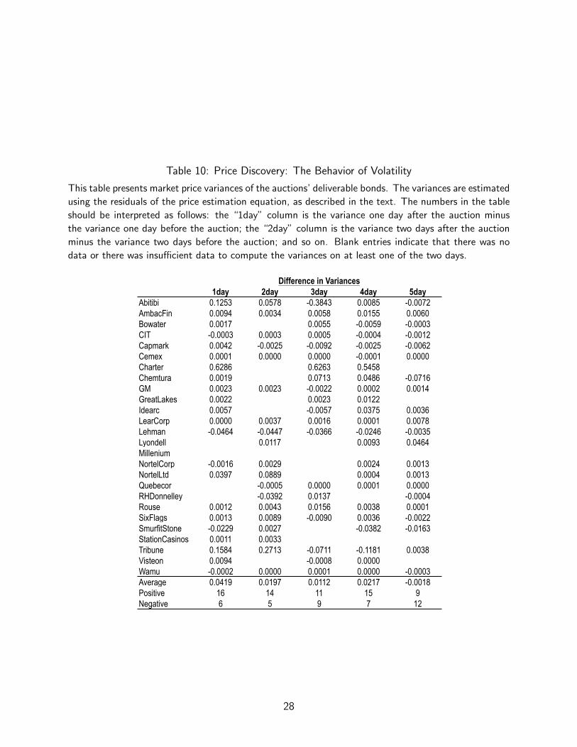
Table 10: Price Discovery: The Behavior of Volatility
This table presents market price variances of the auctions’ deliverable bonds. The variances are estimated
using the residuals of the price estimation equation, as described in the text. The numbers in the table
should be interpreted as follows: the “1day” column is the variance one day after the auction minus
the variance one day before the auction; the “2day” column is the variance two days after the auction
minus the variance two days before the auction; and so on. Blank entries indicate that there was no
data or there was insufficient data to compute the variances on at least one of the two days.
1day 2day 3day 4day 5dayAbitibi 0.1253 0.0578 -0.3843 0.0085 -0.0072AmbacFin 0.0094 0.0034 0.0058 0.0155 0.0060Bowater 0.0017 0.0055 -0.0059 -0.0003CIT -0.0003 0.0003 0.0005 -0.0004 -0.0012Capmark 0.0042 -0.0025 -0.0092 -0.0025 -0.0062Cemex 0.0001 0.0000 0.0000 -0.0001 0.0000Charter 0.6286 0.6263 0.5458Chemtura 0.0019 0.0713 0.0486 -0.0716GM 0.0023 0.0023 -0.0022 0.0002 0.0014GreatLakes 0.0022 0.0023 0.0122Idearc 0.0057 -0.0057 0.0375 0.0036LearCorp 0.0000 0.0037 0.0016 0.0001 0.0078Lehman -0.0464 -0.0447 -0.0366 -0.0246 -0.0035Lyondell 0.0117 0.0093 0.0464MilleniumNortelCorp -0.0016 0.0029 0.0024 0.0013NortelLtd 0.0397 0.0889 0.0004 0.0013Quebecor -0.0005 0.0000 0.0001 0.0000RHDonnelley -0.0392 0.0137 -0.0004Rouse 0.0012 0.0043 0.0156 0.0038 0.0001SixFlags 0.0013 0.0089 -0.0090 0.0036 -0.0022SmurfitStone -0.0229 0.0027 -0.0382 -0.0163StationCasinos 0.0011 0.0033Tribune 0.1584 0.2713 -0.0711 -0.1181 0.0038Visteon 0.0094 -0.0008 0.0000Wamu -0.0002 0.0000 0.0001 0.0000 -0.0003Average 0.0419 0.0197 0.0112 0.0217 -0.0018Positive 16 14 11 15 9Negative 6 5 9 7 12
Difference in Variances
28
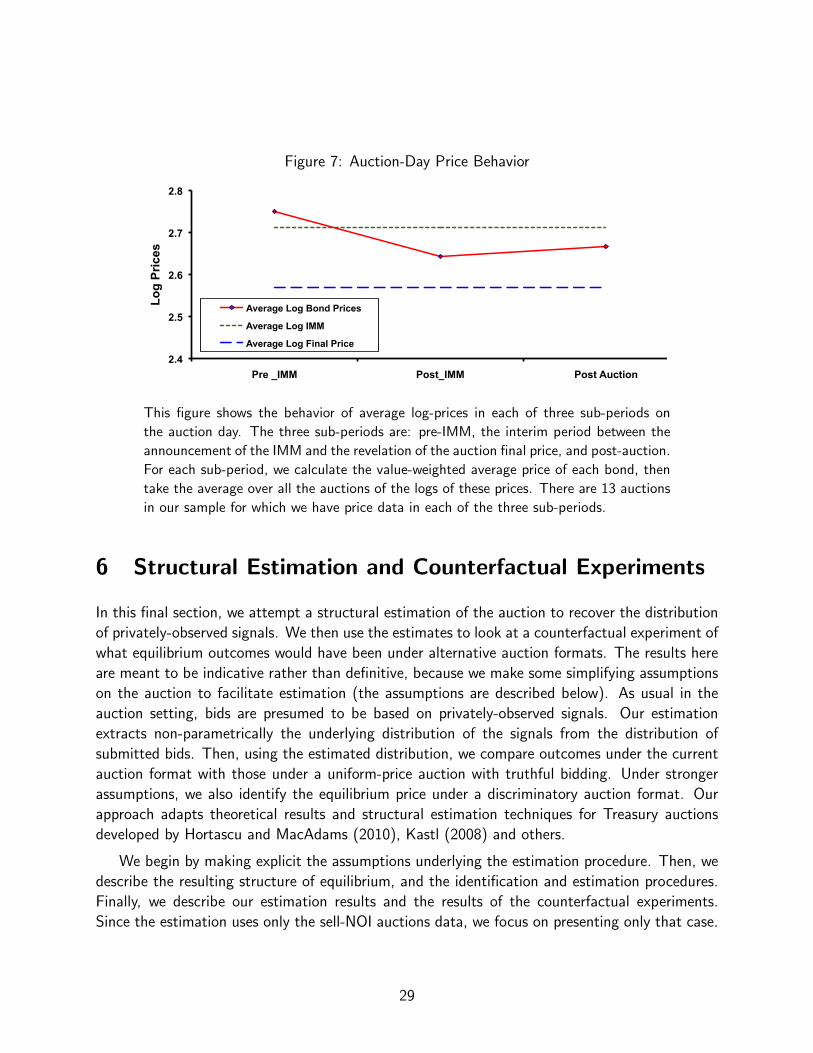
Figure 7: Auction-Day Price Behavior
2.4
2.5
2.6
2.7
2.8
Pre _IMM Post_IMM Post Auction
Log
Pric
es
Average Log Bond Prices
Average Log IMM
Average Log Final Price
This figure shows the behavior of average log-prices in each of three sub-periods on
the auction day. The three sub-periods are: pre-IMM, the interim period between the
announcement of the IMM and the revelation of the auction final price, and post-auction.
For each sub-period, we calculate the value-weighted average price of each bond, then
take the average over all the auctions of the logs of these prices. There are 13 auctions
in our sample for which we have price data in each of the three sub-periods.
6 Structural Estimation and Counterfactual Experiments
In this final section, we attempt a structural estimation of the auction to recover the distribution
of privately-observed signals. We then use the estimates to look at a counterfactual experiment of
what equilibrium outcomes would have been under alternative auction formats. The results here
are meant to be indicative rather than definitive, because we make some simplifying assumptions
on the auction to facilitate estimation (the assumptions are described below). As usual in the
auction setting, bids are presumed to be based on privately-observed signals. Our estimation
extracts non-parametrically the underlying distribution of the signals from the distribution of
submitted bids. Then, using the estimated distribution, we compare outcomes under the current
auction format with those under a uniform-price auction with truthful bidding. Under stronger
assumptions, we also identify the equilibrium price under a discriminatory auction format. Our
approach adapts theoretical results and structural estimation techniques for Treasury auctions
developed by Hortascu and MacAdams (2010), Kastl (2008) and others.
We begin by making explicit the assumptions underlying the estimation procedure. Then, we
describe the resulting structure of equilibrium, and the identification and estimation procedures.
Finally, we describe our estimation results and the results of the counterfactual experiments.
Since the estimation uses only the sell-NOI auctions data, we focus on presenting only that case.
29
Assumptions
The key assumptions underlying our estimation are the following:
1. Dealers are net flat in terms of their CDS exposure entering the auction, and do not submit
physical settlement requests (PSRs) in Round 1. Round 1 PSRs come only from customers.
2. Bond values to dealers have both common value and private value components. The Initial
Market Midpoint (IMM) and the Net Open Interest (NOI) announced prior to Round 2
bidding are sufficient statistics for the common value component of the underlying bonds.
Conditional on the IMM and NOI, dealers have symmetric independent private values drawn
from an identical distribution F before submitting their bids in Round 2.
3. The demand curves submitted in Round 2 are strictly decreasing and continuously differ-
entiable.
4. The observed data comes from a symmetric Bayes Nash equilibrium.
Assumption 1 is based on our discussions with market participants (see Section 2). It implies
that of the quantity and price submissions made in Round 1, only the latter is reflective of the
dealer’s information concerning the bond values. This helps simplify the analysis significantly, as
we can disaggregate the impact of the information component of the dealer with the non-strategic
component (customer orders) of the flow of orders. Assumption 2 is mostly self-explanatory; the
existence of a private value component in bond values may be justified by appealing to dealers’
own risk-management and portfolio considerations that drive their demands for net positions after
the auction. The last part of the assumption helps segregate the influence of others’ signals on
the value function of the dealer. Assumption 3 is important for the identification and estimation
and argument given later in the section. It is only meant to be an approximation, since in reality
dealers submit discrete bids as a step function. Given the symmetry in the assumed structure of
the game, Assumption 4 is a natural condition to impose on equilibrium.
Bidding and Equilibrium
There are n bidders (“players”) in the auction. After the first stage of the auction (in particular,
after observing the IMM), dealer i receives a signal si concerning his private valuation Vi of
the bond. Signals are independent and drawn from identical distributions. Let F (·|IMM) be
the common distribution from which each dealer’s signal is drawn. Given the signal si, dealer
i’s valuation Vi of the bond is a (possibly degenerate) random variable with E[Vi | si, IMM] =
si × IMM. Let L(·|si, IMM) be the distribution of Vi given si and the IMM; note that if L is
degenerate, then we simply have Vi = si×IMM.
30
After observing the signal si, player i submits a demand schedule xi(·; si), where xi(p; si) is
the quantity demanded by i at the price p. Let X = (x1, . . . , xn) denote a vector of strategies and
S = (s1, . . . , sn) a vector of signals. As usual, let X−i and S−i denote the vectors corresponding
to “everyone-but-i,” and let (X−i, yi) denote the vector X but with xi replaced by yi. We restrict
attention to strategies xj that are strictly decreasing and continuously differentiable in p.
For notational ease, we normalize the NOI quantity to 1. Given a vector of strategies X and
a vector of signals S, the price p(X,S) that results in the auction is the value of p that satisfies
n∑i=1
xi(p, si) = 1.
Player i does not know the values of sj for j 6= i, but given (X, si), player i can compute the
auction price p(X, (S−i, si)) that would result for each possible S−i. So from knowledge of the
distribution of signals, i can compute the probability distribution of auction prices that will result
given (X, si). Let H denote the resulting distribution:
H(p |X, si) = Prob (p(X,S) ≤ p |X, si) .
Then, i’s expected profit from the strategy vector X given si is
Πi(X, si) =
∫ [∫(Vi − p)xi(p; si)dH(p |X, si)
]dL(Vi|si). (5)
Player i chooses xi(·; si) to maximize this expected profit for each si. A Nash equilibrium is a
strategy vector X∗ = (x∗1, . . . , x∗n) such that for each i and each si, x
∗i maximizes Π((X−i, yi), si)
over i’s strategy choices yi. Given the symmetric structure of the game, we focus on symmetric
equilibria X∗ = (x∗, . . . , x∗).
Appealing to calculus of variations arguments, Wilson (1979) describes the first-order condi-
tions for the problem of maximizing Π(X, si) over i’s strategy choices xi:
E [(Vi − p)Hp(p|X, si) + xi(p; si)Hx(p|X, si)] = 0,
where the expectation is taken over the distribution L of Vi given si. The only term inside the
expectation that depends on Vi is the first term Vi itself. So we can write this equivalently as
(E[Vi|Si]− p)Hp(p|X, si) + xi(p; si)Hx(p|X, si) = 0,
or, using E(Vi | si) = si× IMM and rearranging,
IMM× si = p− xi(p, .)Hx
Hp
(6)
In equilibrium, each player’s strategy must meet the necessary condition (??). We exploit this
requirement in our estimation procedure below.
31
Identification and Estimation
If the data we observe is generated by the equilibrium of the second stage as described above,
then Condition (6) helps us non-parametrically identify the signals s of the bidders using the
observed bids and the IMM, as we describe here. Define the observed distribution of the residual
supply curve facing a bidder as
G(p, y) = Pr{y ≤ NOI −∑N
j 6=i x(p, sj)}G measures the probability that the quantity demanded x will be less than the (stochastic)
residual supply faced by bidder i. If the joint distribution of {(x(p, sj), j 6= i} can be estimated
from the data, then this probability can be estimated for all (p, x) pairs, and then we have
H[p, x(p, si)] = G(p, y)|y=x(p,si)
Hp =∂
∂pG(p, y)|y=x(p,si)
Hx =∂
∂yG(p, y)|y=x(p,si)
Hence, the signals will be identified from the distribution of observed bids.13
Resampling procedure
Hortacsu and Mcadams (2010) describe an approach for consistently estimating the residual
supply curve for a bidder. We describe their resampling procedure here. Note that due to private
value assumption, each bidder i would care about other’s bidding strategies only through their
impact on the residual supply. Let their be T auctions and N total no of bidders. The following
procedure will consistently estimate the residual supply function for each bidder hence his winning
probability:
• Fix bidder i and a bid xit made by this bidder in an auction t.
• Draw a random subsample of N − 1 bid vectors with replacement from the sample of N
bids in the data set for each auction.
• Construct bidder i’s realized residual supply were others to submit these bids, to determine
the realized market-clearing price given i’s bid xit(.), as well as whether bidder would have
won quantity xit(.) at price pit(.) for all i.
13To be sure, bidders in reality do not submit a strictly downward sloping demand function; rather they submita step function. In such a case, what we identify and estimate here are like bounds of the distribution of signals(Hortacsu and Mcadams, 2010). We abstract away from these considerations.
32
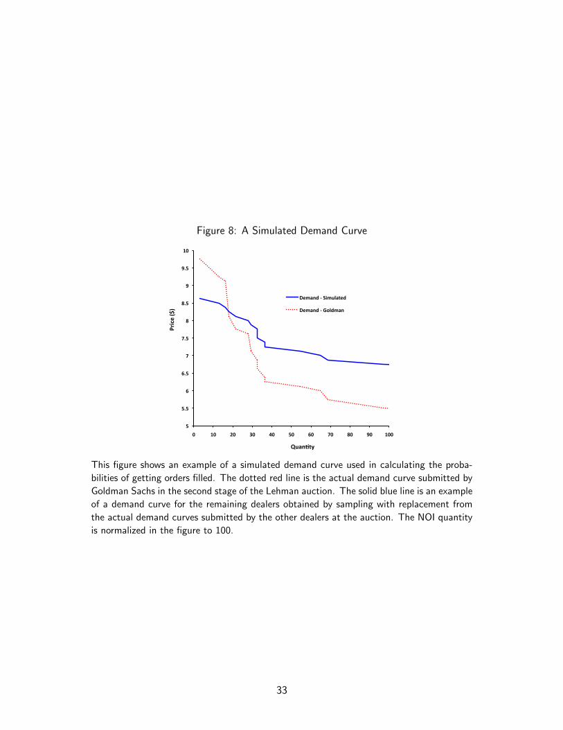
Figure 8: A Simulated Demand Curve
5
5.5
6
6.5
7
7.5
8
8.5
9
9.5
10
0 10 20 30 40 50 60 70 80 90 100
Price ($)
Quan9ty
Demand -‐ Simulated
Demand -‐ Goldman
This figure shows an example of a simulated demand curve used in calculating the proba-
bilities of getting orders filled. The dotted red line is the actual demand curve submitted by
Goldman Sachs in the second stage of the Lehman auction. The solid blue line is an example
of a demand curve for the remaining dealers obtained by sampling with replacement from
the actual demand curves submitted by the other dealers at the auction. The NOI quantity
is normalized in the figure to 100.
33
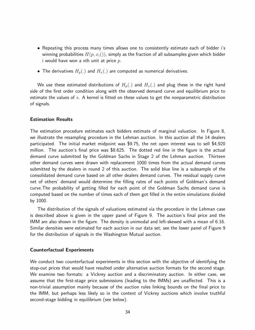
• Repeating this process many times allows one to consistently estimate each of bidder i’s
winning probabilities H(p, xi()), simply as the fraction of all subsamples given which bidder
i would have won a xth unit at price p.
• The derivatives Hp(.) and Hx(.) are computed as numerical derivatives.
We use these estimated distributions of Hp(.) and Hx(.) and plug these in the right hand
side of the first order condition along with the observed demand curve and equilibrium price to
estimate the values of s. A kernel is fitted on these values to get the nonparametric distribution
of signals.
Estimation Results
The estimation procedure estimates each bidders estimate of marginal valuation. In Figure 8,
we illustrate the resampling procedure in the Lehman auction. In this auction all the 14 dealers
participated. The initial market midpoint was $9.75, the net open interest was to sell $4,920
million. The auction’s final price was $8.625. The dotted red line in the figure is the actual
demand curve submitted by the Goldman Sachs in Stage 2 of the Lehman auction. Thirteen
other demand curves were drawn with replacement 1000 times from the actual demand curves
submitted by the dealers in round 2 of this auction. The solid blue line is a subsample of the
consolidated demand curve based on all other dealers demand curves. The residual supply curve
net of others’ demand would determine the filling rates of each points of Goldman’s demand
curve.The probability of getting filled for each point of the Goldman Sachs demand curve is
computed based on the number of times each of them got filled in the entire simulations divided
by 1000.
The distribution of the signals of valuations estimated via the procedure in the Lehman case
is described above is given in the upper panel of Figure 9. The auction’s final price and the
IMM are also shown in the figure. The density is unimodal and left-skewed with a mean of 6.16.
Similar densities were estimated for each auction in our data set; see the lower panel of Figure 9
for the distribution of signals in the Washington Mutual auction.
Counterfactual Experiments
We conduct two counterfactual experiments in this section with the objective of identifying the
stop-out prices that would have resulted under alternative auction formats for the second stage.
We examine two formats: a Vickrey auction and a discriminatory auction. In either case, we
assume that the first-stage price submissions (leading to the IMMs) are unaffected. This is a
non-trivial assumption mainly because of the auction rules linking bounds on the final price to
the IMM, but perhaps less likely so in the context of Vickrey auctions which involve truthful
second-stage bidding in equilibrium (see below).
34
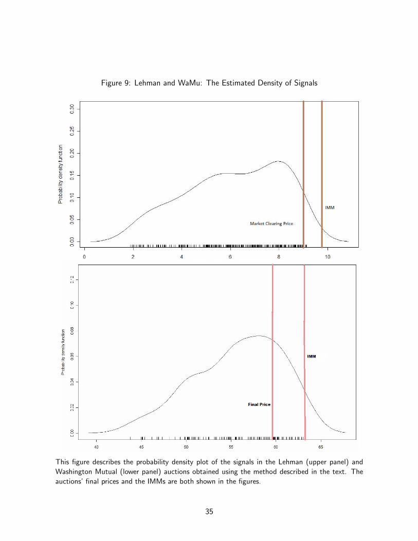
Figure 9: Lehman and WaMu: The Estimated Density of Signals
This figure describes the probability density plot of the signals in the Lehman (upper panel) and
Washington Mutual (lower panel) auctions obtained using the method described in the text. The
auctions’ final prices and the IMMs are both shown in the figures.
35
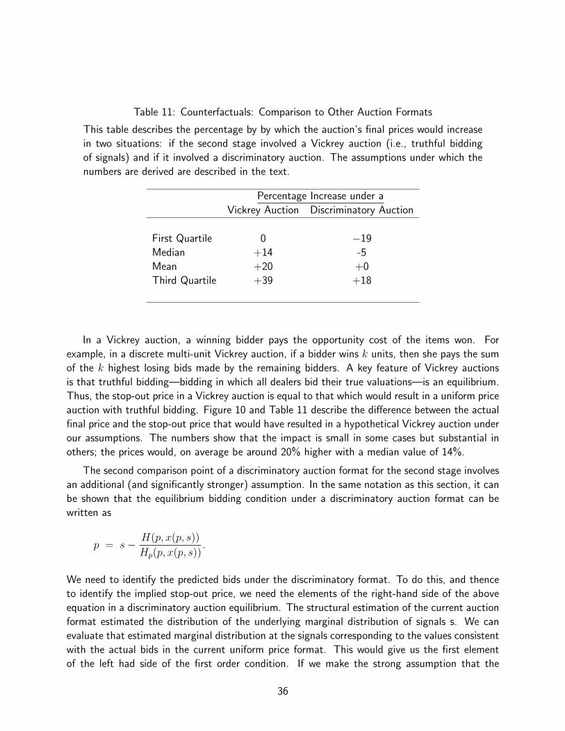
Table 11: Counterfactuals: Comparison to Other Auction Formats
This table describes the percentage by by which the auction’s final prices would increase
in two situations: if the second stage involved a Vickrey auction (i.e., truthful bidding
of signals) and if it involved a discriminatory auction. The assumptions under which the
numbers are derived are described in the text.
Percentage Increase under a
Vickrey Auction Discriminatory Auction
First Quartile 0 −19
Median +14 -5
Mean +20 +0
Third Quartile +39 +18
In a Vickrey auction, a winning bidder pays the opportunity cost of the items won. For
example, in a discrete multi-unit Vickrey auction, if a bidder wins k units, then she pays the sum
of the k highest losing bids made by the remaining bidders. A key feature of Vickrey auctions
is that truthful bidding—bidding in which all dealers bid their true valuations—is an equilibrium.
Thus, the stop-out price in a Vickrey auction is equal to that which would result in a uniform price
auction with truthful bidding. Figure 10 and Table 11 describe the difference between the actual
final price and the stop-out price that would have resulted in a hypothetical Vickrey auction under
our assumptions. The numbers show that the impact is small in some cases but substantial in
others; the prices would, on average be around 20% higher with a median value of 14%.
The second comparison point of a discriminatory auction format for the second stage involves
an additional (and significantly stronger) assumption. In the same notation as this section, it can
be shown that the equilibrium bidding condition under a discriminatory auction format can be
written as
p = s− H(p, x(p, s))
Hp(p, x(p, s)).
We need to identify the predicted bids under the discriminatory format. To do this, and thence
to identify the implied stop-out price, we need the elements of the right-hand side of the above
equation in a discriminatory auction equilibrium. The structural estimation of the current auction
format estimated the distribution of the underlying marginal distribution of signals s. We can
evaluate that estimated marginal distribution at the signals corresponding to the values consistent
with the actual bids in the current uniform price format. This would give us the first element
of the left had side of the first order condition. If we make the strong assumption that the
36

Figure 10: Counterfactual I: The Impact of Vickrey Auctions
The figure presents the estimated percentage increase in prices that would result
for each auction if the second-stage of the auction involved truthful bidding.
0.00%
20.00%
40.00%
60.00%
80.00%
100.00%
Que
becor
Millen
ium
Capm
ark
Glitnir
Idearc CDS
Kaup
thing
Rouse
Truvo
Kaup
thing Seno
r Glitnir Subo
rdinated
NaH
ogaz
Washington Mutua
l Nortel Corp
Lehm
an Brothers
EquitStar
CIT
Takefuji
Tembe
c Hellas
Nortel Ltd.
Brad
ford
R. H. D
onne
lley
Thom
son
Smurfit-‐Stone
CDS
Average
Amba
c Fina
ncial
Great Lakes
Aifu
l JSC
Visteon
CDS
Lear Corp CD
S Lyon
dell CD
S Ch
emtura
Lyon
dell Ba
sell
Amba
c Assuran
ce
Land
sban
ki Sen
ior
Tribun
e CD
S Japa
n Airlin
es
function H(·) is the same under the two formats, then we can use our current estimated of H
and Hp through the resampling procedure described before to arrive at the predicted bids under
the discriminatory format. Carrying this out and examining the impact, Table 11 shows that on
average there is no impact (0%), while the mean impact is −5%.
7 Conclusion
This paper provides the first detailed empirical analysis of the auction mechanism used to settle
credit default swaps after a credit event. We find that the auction price has a significant bias
relative to the pre- and post-auction bond prices. Nonetheless, econometric analysis shows that
auction-identified information, and in particular, the auction’s final price, is critical to post-auction
price formation. Bidder behavior and auction outcomes are significantly affected by winner’s curse
and strategic considerations, providing at least a partial explanation of the observed price bias.
Somewhat surprisingly, and at first sight, inconsistently with price discovery, we find that volatility
of bond prices actually increases after the auction, but this may just indicate the presence of new
informed investors who enter only post-auction. Finally, we also carry out a limited structural
37
estimation of the auction aimed at uncovering the distribution of signals that guides auction
behavior; under some (relatively strong) assumptions, we use the identified signals to see the
potential price effects of changing the auction format.
Several interesting avenues of research remain to be investigated. One is the development
of a complete theoretical model of credit-event auctions. Promising bases have been laid in this
direction by the work of Du-Zhu (2010) and especially Chernov, et al (2011); an important issue
that remains is to incorporate asymmetric information aspects into the model. A second, coming
out of the first, is a more complete structural estimation of the auction. And finally, building on
both of these, is the identification of potentially better auction mechanisms.
38
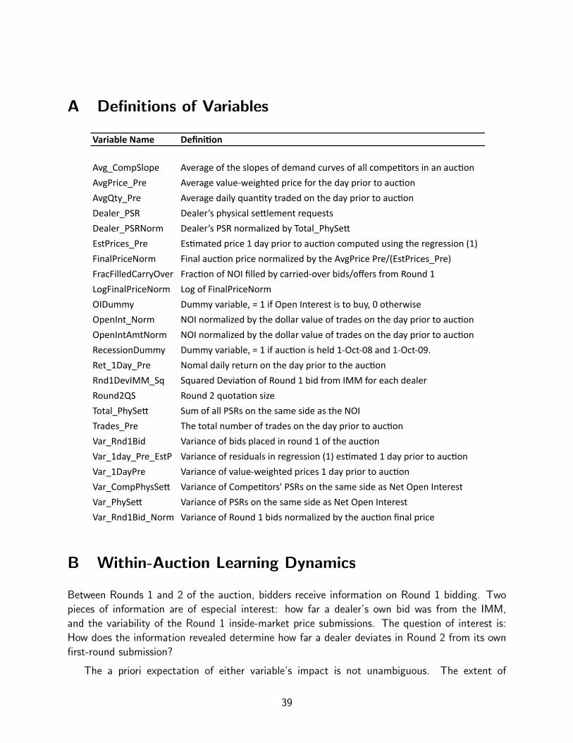
A Definitions of Variables
Variable Name Defini.on
Avg_CompSlope Average of the slopes of demand curves of all compe7tors in an auc7on
AvgPrice_Pre Average value-‐weighted price for the day prior to auc7on
AvgQty_Pre Average daily quan7ty traded on the day prior to auc7on
Dealer_PSR Dealer’s physical seBlement requests
Dealer_PSRNorm Dealer’s PSR normalized by Total_PhySeB
EstPrices_Pre Es7mated price 1 day prior to auc7on computed using the regression (1)
FinalPriceNorm Final auc7on price normalized by the AvgPrice Pre/(EstPrices_Pre)
FracFilledCarryOver Frac7on of NOI filled by carried-‐over bids/offers from Round 1
LogFinalPriceNorm Log of FinalPriceNorm
OIDummy Dummy variable, = 1 if Open Interest is to buy, 0 otherwise
OpenInt_Norm NOI normalized by the dollar value of trades on the day prior to auc7on
OpenIntAmtNorm NOI normalized by the dollar value of trades on the day prior to auc7on
RecessionDummy Dummy variable, = 1 if auc7on is held 1-‐Oct-‐08 and 1-‐Oct-‐09.
Ret_1Day_Pre Nomal daily return on the day prior to the auc7on
Rnd1DevIMM_Sq Squared Devia7on of Round 1 bid from IMM for each dealer
Round2QS Round 2 quota7on size
Total_PhySeB Sum of all PSRs on the same side as the NOI
Trades_Pre The total number of trades on the day prior to auc7on
Var_Rnd1Bid Variance of bids placed in round 1 of the auc7on
Var_1day_Pre_EstP Variance of residuals in regression (1) es7mated 1 day prior to auc7on
Var_1DayPre Variance of value-‐weighted prices 1 day prior to auc7on
Var_CompPhysSeB Variance of Compe7tors' PSRs on the same side as Net Open Interest
Var_PhySeB Variance of PSRs on the same side as Net Open Interest
Var_Rnd1Bid_Norm Variance of Round 1 bids normalized by the auc7on final price
B Within-Auction Learning Dynamics
Between Rounds 1 and 2 of the auction, bidders receive information on Round 1 bidding. Two
pieces of information are of especial interest: how far a dealer’s own bid was from the IMM,
and the variability of the Round 1 inside-market price submissions. The question of interest is:
How does the information revealed determine how far a dealer deviates in Round 2 from its own
first-round submission?
The a priori expectation of either variable’s impact is not unambiguous. The extent of
39
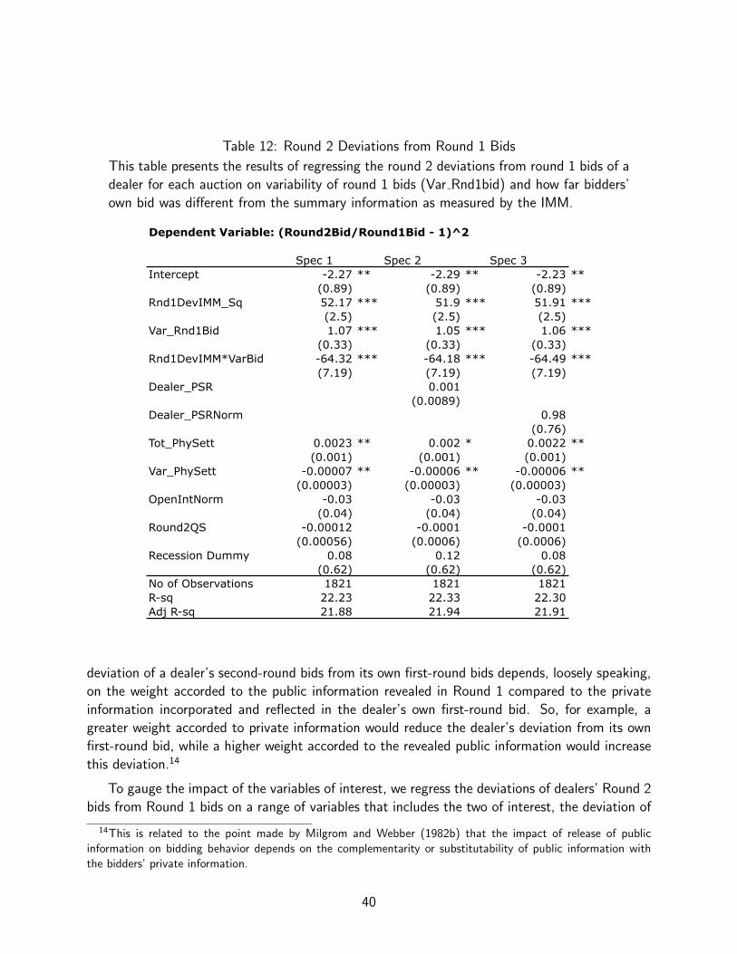
Table 12: Round 2 Deviations from Round 1 Bids
This table presents the results of regressing the round 2 deviations from round 1 bids of a
dealer for each auction on variability of round 1 bids (Var Rnd1bid) and how far bidders’
own bid was different from the summary information as measured by the IMM.
Dependent Variable: (Round2Bid/Round1Bid - 1)^2
Spec 1 Spec 2 Spec 3Intercept -2.27 ** -2.29 ** -2.23 **
(0.89) (0.89) (0.89)Rnd1DevIMM_Sq 52.17 *** 51.9 *** 51.91 ***
(2.5) (2.5) (2.5)Var_Rnd1Bid 1.07 *** 1.05 *** 1.06 ***
(0.33) (0.33) (0.33)Rnd1DevIMM*VarBid -64.32 *** -64.18 *** -64.49 ***
(7.19) (7.19) (7.19)Dealer_PSR 0.001
(0.0089)Dealer_PSRNorm 0.98
(0.76)Tot_PhySett 0.0023 ** 0.002 * 0.0022 **
(0.001) (0.001) (0.001)Var_PhySett -0.00007 ** -0.00006 ** -0.00006 **
(0.00003) (0.00003) (0.00003)OpenIntNorm -0.03 -0.03 -0.03
(0.04) (0.04) (0.04)Round2QS -0.00012 -0.0001 -0.0001
(0.00056) (0.0006) (0.0006)Recession Dummy 0.08 0.12 0.08
(0.62) (0.62) (0.62)No of Observations 1821 1821 1821R-sq 22.23 22.33 22.30Adj R-sq 21.88 21.94 21.91
deviation of a dealer’s second-round bids from its own first-round bids depends, loosely speaking,
on the weight accorded to the public information revealed in Round 1 compared to the private
information incorporated and reflected in the dealer’s own first-round bid. So, for example, a
greater weight accorded to private information would reduce the dealer’s deviation from its own
first-round bid, while a higher weight accorded to the revealed public information would increase
this deviation.14
To gauge the impact of the variables of interest, we regress the deviations of dealers’ Round 2
bids from Round 1 bids on a range of variables that includes the two of interest, the deviation of
14This is related to the point made by Milgrom and Webber (1982b) that the impact of release of publicinformation on bidding behavior depends on the complementarity or substitutability of public information withthe bidders’ private information.
40
a dealer’s own Round 1 bid from the IMM, and the variability of first-round bids, as well as an
interaction term between the two. Our findings, reported in Table 12, point to effects that are
both subtle and interesting.
On the one hand, the coefficients on both terms, the Round 1 deviation of one’s own bid
from the IMM and the variability of Round 1 bids, are both positive and highly significant. This
likely signifies the the incorporation of and greater weight accorded to public information into
second-round bids. (For example, a higher deviation of a dealer’s own bid from the IMM leads to
increased weight on the revealed public information will lead to a higher deviation of the dealer’s
second-round bid from the first-round bid.) On the other hand, the coefficient on the interaction
term is negative, and is also large and significant. This means that the marginal impact of (say)
the Round 1 deviation from IMM depends on the variability of Round 1 bids, and so the possibility
of a winner’s curse effect. For example, if we evaluate this marginal impact at the first quartile of
variability bidders’ Round 1 bids, we find that the overall impact is positive; bidders adjust their
Round 2 bids based on the consensus. However if we do the evaluation at the median variability
level of Round 1 bids (roughly, 0.7), then the overall impact is negative. Intuitively, the increased
winner’s curse impact causes bidders to put more weight on their private information and not
deviate too much from their own first-round bids.
41

References
Back, Kerry and Jaime Zender (1993) Auctions of Divisible Goods: The Rationale for the
Treasury Experiment, Revew of Financial Studies 6(4), 733-764.
Bajari, Patrick and Ali Hortacsu (2005) Are Structural Estimates of Auction Models Reasonable?
Evidence from Experimental Data, Journal of Political Economy 113(4), 703-741.
Coudert, Virginie and Matthieu Gex (2010) The Credit-Default Swap Market and the Settlement
of Large Defaults, CEPII Working Paper 2010-17.
Das, Sanjiv R. and Rangarajan K. Sundaram (1996) Auction Theory: A Survey with Applications
to Treasury Markets, Financial Markets, Institutions, and Instruments 5(5), 1-36.
Das, Satyajit (2010) The Credit Default Swap (“CDS”) Market—Will It Unravel?, accessed on-
line at http://www.wilmott.com/blogs/satyajitdas/index.cfm/2008/5/30/The-Credit-Default-
Swap-CDS-Market–Will-It-Unravel.
Chernov, Mikhail; Alexander S. Gorbenko and Igor Makarov (2011) CDS Auctions, mimeo,
London School of Economics and London Business School.
Du, Songzi and Haoxiang Zhu (2011) Are CDS Auctions Biased? mimeo, Graduate School of
Business, Stanford University.
Helwege, Jean; Samuel Maurer, Asani Sarkar, and Yuan Wang (2009) Credit Default Swap
Auctions, Staff Report No. 372, Federal Reserve Bank of New York.
Hortacsu, Ali and David McAdams (2010) Mechanism Choice and Strategic Bidding in Divisible-
Good Auctions: An Empirical Analysis of the Turkish Treasury Auction Market, Journal of
Political Economy 118(5), pp. 833-65.
Kastl, Jakub (2008) On the Properties of Equilibria in Private Value Divisible-Good Auctions
with Constrained Bidding, Working Paper, Stanford University.
Keloharju, Matti; Kjell Nyborg, and Kristian Rydqvist (2005) Strategic Behaviour and Under-
pricing in Uniform Price Auctions: Evidence from Finnish Treasury Auctions, Journal of
Finance 60(4), 1865-1902.
Kremer, Ilan and Kjell G. Nyborg (2004) Underpricing and Market Power in Uniform Price
Auctions, Review of Financial Studies 17, pp. 849-877.
McAfee, R. Preston and John McMillan (1987) Auctions and Bidding, Journal of Economic
Literature, 699-738.
42
Milgrom, Paul R. and Robert J. Webber (1982) A Theory of Auctions and Competitive Bidding,
Econometrica, 1089-1122.
Milgrom, Paul R. and Robert J. Webber (1982b) The Value of Information in a Sealed-Bid
Auction, Journal of Mathematical Economics 10(1), 105-114.
Nyborg, Kjell; Kristian Rydqvist, and Suresh M. Sundaresan (2002) Bidder Behavior in Multiunit
Auctions: Evidence from Swedish Treasury Auctions, Journal of Political Economy 110(2),
394-424.
Nyborg, Kjell and Suresh M. Sundaresan (1996) Discriminatory versus Uniform-Price Treasury
Auctions: Evidence from When-Issued Transactions, Journal of Financial Economics 42,
pp. 63-104.
Summe, Kimberly and David Mengle (2006) Settlement of Credit Default Swaps: Mechan-
ics, Challenges, and Solutions, Presentation made at the Credit Derivative Symposium,
Fordham Graduate School of Business, September 29, 2006.
Wilson, Robert (1979) Auctions of Shares, Quarterly Journal of Economics 93, 675-689.
Ye, Lixin (2007) Indicative Bidding and a Theory of Two-Stage Auctions, Games and Economic
Behavior 58(1), 181-207.
43