argovis: a web application for fast delivery

Argovis: A Web Application for Fast Delivery, Visualization, and Analysis of Argo Data

TYLER TUCKER

Department of Atmospheric and Oceanic Sciences, University of Colorado Boulder, Boulder, Colorado, and

Department of Mathematics and Statistics, San Diego State University, San Diego, and Scripps Institution of Oceanography,

University of California, San Diego, La Jolla, California

DONATA GIGLIO

Department of Atmospheric and Oceanic Sciences, University of Colorado Boulder, Boulder, Colorado

MEGAN SCANDERBEG

Scripps Institution of Oceanography, University of California, San Diego, La Jolla, California

SAMUEL S. P. SHEN

Department of Mathematics and Statistics, San Diego State University, San Diego, California

(Manuscript received 18 March 2019, in final form 3 January 2020)

ABSTRACT

Since the mid-2000s, the Argo oceanographic observational network has provided near-real-time four-

dimensional data for the global ocean for the first time in history. Internet (i.e., the ‘‘web’’) applications that

handle themore than twomillionArgo profiles of ocean temperature, salinity, and pressure are an active area

of development. This paper introduces a new and efficient interactive Argo data visualization and delivery

web application named Argovis that is built on a classic three-tier design consisting of a front end, back end,

and database. Together these components allow users to navigate 4D data on a worldmap ofArgo floats, with

the option to select a custom region, depth range, and time period. Argovis’s back end sends data to users in a

simple format, and the front end quickly renders web-quality figures. More advanced applications query

Argovis from other programming environments, such as Python, R, andMATLAB.OurArgovis architecture

allows expert data users to build their own functionality for specific applications, such as the creation of

spatially gridded data for a given time and advanced time–frequency analysis for a space–time selection.

Argovis is aimed to both scientists and the public, with tutorials and examples available on the website,

describing how to use the Argovis data delivery system—for example, how to plot profiles in a region over

time or to monitor profile metadata.

1. Introduction

For the first time in history, the Argo network of

profiling floats provides real-time data of temperature

T, salinity S, and pressure P for the global ocean to a

depth of 2000 dbar, with Deep Argo floats going down

to 6000-dbar depth. Argo floats have been deployed

since the early 2000s and reached the expected spatial

distribution in 2007 (Roemmich et al. 2009). Nearly

4000 floats are currently operating in the global ocean

and provide a profile every 10 days, that is, measure-

ments from a vertical column of the ocean as a single

float ascends to the surface. The four-dimensional (4D)

space–time Argo data have many scientific and tech-

nological advantages, two of which are 1) unprece-

dented spatial and temporal resolution over the global

ocean, and 2) no seasonal bias (Roemmich et al. 2009).

More than two million T/S/P profiles have been col-

lected through the Argo Program. Datasets as complex

and large as Argo raise data delivery and visualization

challenges. Users need to extract relevant subsets without

necessarily having the expertise and familiarity with data

formatting practices or programming knowledge.

Denotes content that is immediately available upon publica-

tion as open access.

Corresponding author: Tyler Tucker, [email protected]

MARCH 2020 TUCKER ET AL . 401

DOI: 10.1175/JTECH-D-19-0041.1

� 2020 American Meteorological Society. For information regarding reuse of this content and general copyright information, consult the AMS CopyrightPolicy (www.ametsoc.org/PUBSReuseLicenses).

Dow

nloaded from http://journals.am

etsoc.org/jtech/article-pdf/37/3/401/4933825/jtechd190041.pdf by University of C

olorado Libraries user on 02 July 2020

mailto:[email protected]

http://www.ametsoc.org/PUBSReuseLicenses



The International Argo Program, plus the national

programs that contribute to it, makes Argo data avail-

able online to anyone, with global data assembly centers

(GDACs; for convenience, the acronyms and abbrevi-

ations used in this paper are also defined in Table 1)

storing the data online. Users download either single

profiles or all of the profiles taken from a single float

over its entire history of deployment. With little option

of space–time or metadata selection, this method is in-

efficient for many scientific and/or technical applications

and discourages use by laypeople and policy makers.

An ongoing effort has been made within the Argo

community to improve visualization and delivery of

Argo data and their derivative products to scientists,

policy makers, and the general public. Some visualiza-

tion tools are currently available online. For example,

the Joint Technical Commission for Oceanography and

Marine Meteorology In Situ Observations Programme

Support Centre (JCOMMOPS) includes an interactive

map (at http://argo.jcommops.org) that prompts users to

query floats by program (Core Argo, Biogeochemical

Argo, Deep Argo, etc.), nation, float type, last position,

transmission type, and so on (JCOMMOPS 2019). The

most recent profile of the selected floats appears on the

interactive map with the option to show all positions of

profiles within a size limit. TheArgo-France group offers a

TABLE 1. List of abbreviations along with context of how they apply to this paper.

Abbreviation Definition Explanation

ASCII American Standard Code for

Information Interchange

A file that contains unformatted text is called an ASCII or text file

API Application programming

interface

A set of methods of communication among various computers; in the context

of this paper, it allows software programs to request data from Argovis

BGC Biogeochemical Argo floats that are equipped with additional sensors that measure BGC

parameters, such as dissolved oxygen

CPU Central processing unit A microprocessor that is often described as the brain of a computer; it

specializes in sequential computing

CSS Cascading Style Sheets A language used for describing the presentation of elements on an HTML

document

CSV Comma-separated value A file type that stores tabular data in plain text, delimited by a separator

(such as a comma)

DAC Data assembly center National DACs gather and perform QC on floats owned by that nation

dbar Decibar Unit of pressure; 1 dbar is approximately equal to 1-m depth of seawater

FTP File transfer protocol A standard network protocol used to transfer files on a computer network

GDACs Global DAC GDACs store and maintain Argo data sent by DACS

GPS Global positioning system A satellite-based radionavigation system that some Argo floats use to

communicate with their respective DACs

GPU Graphics processing unit A microprocessor that specializes in parallel computing, such as rendering

graphics

HTML Hypertext Markup Language A language for documents designed to be displayed in a web browser; often

used with CSS and JavaScript

HTTP Hypertext Transfer Protocol ‘‘HTTP is the underlying protocol used by the [web; it] defines how messages

are formatted and transmitted, and what actions web servers and browsers

should take in response to various commands’’ (V. Beal; https://www.

webopedia.com/TERM/H/HTTP.html)

JSON JavaScript Object Notation An open-standard file format text to transmit data objects consisting of

key-value pairs

KML Keyhole Markup Language A file type for expressing geographic annotation and visualization within

Google Earth

NetCDF Network Common Data Form A type of file designed to house array-oriented scientific data

QC Quality control The process of assigning a ranking at which processed Argo data are rated

RESTful Representational State Transfer A software architectural style that defines a set of constraints to be used for

creating web services; Argovis is RESTful because 1) it uses a base URL,

2) it has an API interface that accepts ‘‘GET’’ requests, and 3) it sends

data as JSON

SQL Structured Query Language A language used to create, maintain, and retrieve relational databases such

as MySQL or Postgres

T/S/P Temperature, salinity, and pressure Core variables measured by each Argo float

URL Uniform resource locator An address identifying where documents or web pages can be found on the

Internet

WMO World Meteorological Organization Argo floats are designated by a unique WMO number

402 JOURNAL OF ATMOSPHER IC AND OCEAN IC TECHNOLOGY VOLUME 37

Dow




http://argo.jcommops.org

https://www.webopedia.com/TERM/H/HTTP.html

https://www.webopedia.com/TERM/H/HTTP.html

product (at http://map.argo-france.fr/) that shows profile

locations for the past 7 days with the option to click on

individual profiles and see a plot of the data and previous

locations for that float (ArgoFrance 2019).Also, theEuro-

Argo group offers a similar Argo visualization application

(at https://fleetmonitoring.euro-argo.eu/dashboard).

There are data delivery tools (for data other than

Argo) whose design the Argo Program can borrow for

their own application. The Web-Based Reanalyses

Intercomparison Tools (WRIT) (at https://www.esrl.

noaa.gov/psd/data/writ/) (Smith et al. 2014) allow users to

create customized plots and retrieve climate data from

these plots. WRIT addresses how to store and distribute

large climate datasets, and helps to overcome data selec-

tion and delivery for scientists. The complex tabularWRIT

interface is for scientists and professionals and not for the

general public or, for example, high-school students.

A similar application is owned by NASA GES DISC.

Giovanni (at https://giovanni.gsfc.nasa.gov/giovanni/),

uses a dedicated server to create images, Keyhole

Markup Language (KML) files used by Google Maps,

and Network Common Data Form (netCDF) files.

Giovanni depends on a server to handle WorldWide

Web (hereinafter the ‘‘web’’) traffic, which requires

hardware and maintenance. Alternatively, using the

user’s browser to generate plots and maps significantly

reduces computational loads, thereby reducing the re-

sources needed to host a data delivery web application.

The Four-Dimensional Visual Delivery (4DVD)

technology (at http://4dvd.sdsu.edu/) (Pierret and Shen

2017) is one such tool: it combines data visualization

and delivery while also having the user’s computer

create customized charts and maps. 4DVD displays

gridded data and time series on an interactive globe for

Global Precipitation Climatology Project (GPCP) data

and NOAA CIRES reanalysis fields. Users make se-

lections on a menu such as depth and date, to display

data dynamically. Visualization elements such as charts

andmaps are rendered using the user’s central processing

unit (CPU) and graphics processing unit (GPU). This

allows the webserver to focus on sending data quickly,

requiring little computation power and ultimately im-

proving its performance (Pierret and Shen 2017).

Following the ideas of the 4DVD technology, we

created Argovis (at https://argovis.colorado.edu), a

modern and efficient web application that combines

web browser, webserver, and database technologies to

navigate the Argo dataset in space and time. This web

application provides two services: 1) visualizing Argo

data and its gridded products with charts and maps

and 2) delivering Argo data to the user. Through basic

web browser navigation, Argovis enables a wide va-

riety of users to use a world map of Argo floats, a

depth range, and a time range to request, visualize,

and analyze the 4D Argo data stored in an optimized

database. The fast Argovis database enables users to receive

JavaScript Object Notation (JSON) or comma-separated

value (CSV) formatted data and Hypertext Markup

Language (HTML) figures almost instantly. More advanced

users can also query Argovis from other programming en-

vironments, such as Python, R, and MATLAB.

Argovis improves on other tools for Argo data access

by allowing interactive querying and visualizing of cu-

rated profiles on the basis of a 4D spatial–temporal data

selection (e.g., retrieving upper-ocean data in the trop-

ical eastern Pacific Ocean during a period of interest).

In addition, metadata database queries and additional

specialized aggregation queries are under development.

The guiding philosophy of our Argovis development

includes visualization with minimal effort, fast delivery,

and wide availability for everyone. We referenced the

ideas of an interactive and responsive interface for

children, making Argovis attractive, self-explainable,

and 4D. Argovis is different from the traditional data

service technologies, such as file transfer protocol (FTP)

and download that passively feed digital data to a user or

consume the server’s computing resources to generate

and push figures (e.g., the NASAGiovanni application).

The Argovis system is an active technology instead,

displaying data dynamically. The user requests data that

are used to render pages on the browser.

For data science experts, our architecture allows for

statistical analysis such as optimal interpolation (also

known as objectivemapping or statistical interpolation),

for example, to calculate sea surface height anomalies

using Argo temperature and salinity profile data as in

Kuragano et al. (2015). Kuragano et al.’s (2015) model

depends on fitting a local 3D Gaussian function regu-

lated by small scales, and can represent an anisotropic

spatial scale, time scale, and propagation feature of

oceanographic variability. The data used to calculate

parameters scales for the Gaussian function are gridded

(1/48 latitude 3 longitude 3 3 days), requiring hundreds

of thousands of data queries. Argovis’s application

programming interface (API) querying tool can be very

helpful in this instance. In more general terms, Argovis’s

API makes the process of selecting Argo data flexible

and customizable to the needs of each model or re-

searcher. As an interface to a database, the API is de-

signed for such queries, so that datamanipulation time is

reducedwhile simultaneously relieving the researcher of

the task of optimizing data input or output. The API can

also be used for data extraction to create gridded

products using other methods, for example, objective

mapping in Roemmich and Gilson (2009) or Kuusela

and Stein (2018) or spectral optimal gridding in Shen


Dow




http://map.argo-france.fr/

https://fleetmonitoring.euro-argo.eu/dashboard

https://www.esrl.noaa.gov/psd/data/writ/

https://www.esrl.noaa.gov/psd/data/writ/

https://giovanni.gsfc.nasa.gov/giovanni/

http://4dvd.sdsu.edu/

https://argovis.colorado.edu

et al. (2017). More of this will be covered in the space–

time query section described in section 6c. For users

interested, instead, in analyzing profiles locations,

dates, DACs, positioning systems, and so on, we have

provided a metadata API, whose details and example

applications are explained in section 6d.

In the following sections, we recapitulate the Argo

network and its data in section 2 and provide an overview

of the web application in section 3. Design practices rel-

evant to Argovis are covered in section 4. Section 5

provides technical details of Argovis, addressing how the

database is structured (section 5a), how datasets are

added to the database (section 5a), and how the database

is connected (section 5b). Section 6 describes how

Argovis data are accessed both through the interface for

the website (https://argovis.colorado.edu) and through

theAPI. Section 7 presents the summary and conclusions.

As supplementary materials to this paper, Argovis tuto-

rials have been developed and are freely available via the

tutorial link on the Argovis home page.

Argovis current uniform resource locator (URL) (https://

argovis.colorado.edu) is referenced in this paper. Future

changes to the application domain name will be mentioned

in the ‘‘README’’ file of the Argovis GitHub repository

(https://github.com/tylertucker202/argo-database). Up-to-

date URLs for Argovis API can be found via the tutorial

link on the Argovis home page.

2. The Argo data network

Most Argo floats drift at a parking depth of 1000dbar

and make T/S/P measurements every 10 days while

rising to the surface (from a profiling depth of 2000dbar).

A limited number of floats include biogeochemical ob-

servations (Claustre et al. 2010; Gruber et al. 2010) and or

measure deeper than 2000dbar (e.g., to depths of

6000dbar). Once at the surface, Argo floats transmit

profile data to national data assembly centers (DACs).

These raw measurements undergo automated quality

control (QC) tests and adjustments before being sent as

netCDF files to the GDACs where they are served on

FTP servers. Servers are frequently updated to include

additional QC checks by a float’s primary investigator.

Profile data that undergo automatic QC are known as

real-time-mode profiles. Profiles that are inspected by

oceanographic experts and passed through an adjustment

algorithm (described in Owens and Wong 2009), are

known as delayed-mode profiles. The observational cycle

of an Argo float produces a data profile. More than two

million profiles have been collected through the Argo

Program since 2000, and navigating through the large and

complex Argo dataset can be challenging. For instance,

accessing Argo netCDF files on the GDACs involves

parsing through a remote or local archive of files, selecting

relevant files, opening the files, and performing analysis.

As an alternative, Argovis takes profile data from the

GDACs and stores them on a database that is coupled

with a front-end interface for charting and data delivery.

3. Web application overview

The Argovis main web page, shown in Fig. 1, con-

sists of an interactive map and sidebar with controls,

allowing users an intuitive way to navigate through

profiles, either by a space–time query or by entering a

float’s World Meteorological Organization (WMO)

number. Argovis home page shows the interactive

map, along with the locations of profiles in a 3-day

window (whose latest date defaults to ‘‘yesterday’’

and can be changed in the side panel). The interactive

map is created using the Leaflet.js library, that is, a

tiledwebmapgenerator that includes plugin extensions for

shapes and images to be displayed on web maps. Clicking

and dragging the map pans the view, and zooming can be

done by double clicking a spot on the map.

Toggle elements are included in the sidebar, allowing

a quick filter for special types of profiles, such as

‘‘Biogeochemical’’ (BGC) or ‘‘Deep’’ floats. Note that

these types of floats appear as different colors. BGC

floats are displayed as green, and Deep floats are dis-

played in dark blue, in contrast to the standard yellow

profiles. A button on the side panel clears the page from

all the profile locations (i.e., all the dots), if needed (e.g.,

before a selection).

The pop-up window that appears when a dot is clicked

contains the latitude and longitude coordinates, the

profile’s measurement date, and a button that will show

the float’s previous profile locations (see the pop-up in

Fig. 2a). Links to either the profile page (shown in

Fig. 3a) or the entire float history (shown in Fig. 2b) are

included as well. BGC floats have links to their own page

displaying additional parameters. Another way to view a

float’s trajectory is by typing in the platform’s WMO

number on the side panel, revealing the platform’s his-

tory as seen in Fig. 2a.

Different map projections are available by clicking

the name of the desired projection near the top of the

sidebar. Currently, web Mercator, northern stereo-

graphic, and southern stereographic are the only

projections available. Only web Mercator uses map

tiles; the latter two use a JSON shapefile to show land

outlines (see Fig. 2a for a southern stereographic

projection map).

In each projection, the map includes a drawing plug-

in that allows users to create, edit, and delete a po-

lygonal region of interest. When a polygon is created


Dow







https://github.com/tylertucker202/argo-database

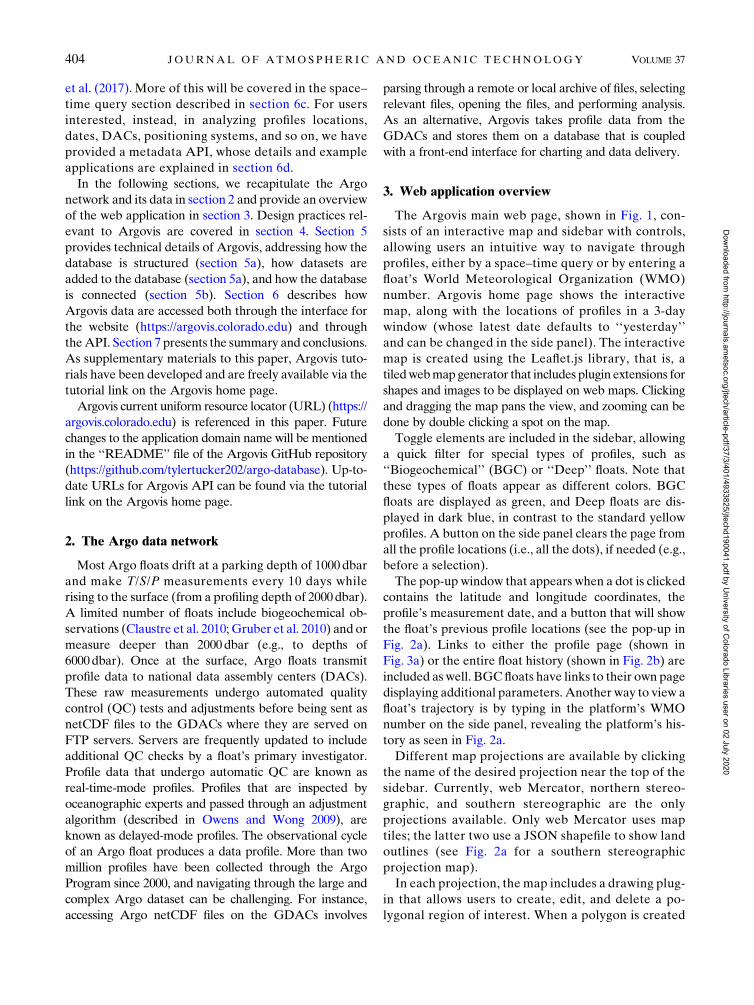
by drawing it on the map, the application queries the

database for profiles falling within the region bounded

by the polygon, along with the date and pressure

ranges selected on the side panel. If the query is not

too large, the application clears the map of profiles

and displays profiles that match the temporal–spatial

query returned by the database (Fig. 4a). If the query

is too large, a message warns the user, with a sugges-

tion to explore API options. The completed shape

(e.g., Fig. 4a) will also have a pop-up window with two

buttons that open web pages with T/S/P plots for the

region and period of interest, with or without the

pressure selection (Fig. 4b). The T/S/P plots are in-

teractive and when you click on one profile, a new web

page opens showing the T/S/P plots for that single

profile (Fig. 3a) and a link to plots for the platform

history (Fig. 2b).

Below the T/S/P plots for a drawn section or a

platform, there is a table and several buttons for data

or table downloading (Fig. 4b). The columns in Fig. 4c

are sorted by latitude, longitude, data center, data

mode, positioning system, and so on. To access the

same region frequently, a user can simply copy the

URL of the selection region and reuse it as desired.

The date can be changed in the URL link for a dif-

ferent time period.

4. Overview of the Argovis web application design

Modern web framework design and practices pair well

with large climate and oceanographic data. Argovis only

uses free and open sourced software that are actively de-

veloped and maintained by a community of developers.

The tools used to create the Argovis interface as

shown in Fig. 1 came from a standard web application

design. Web pages are built with HTML and styled

with Cascading Style Sheets (CSS). Together these

languages display images, buttons, tables, pop-up

windows, and so on but do not address event han-

dling such as clicking or scrolling. Logic and event

handling are done with JavaScript, which handles the

position and zoom level of the map global view. Users

import and run HTML, CSS, and JavaScript on their

browser as the front end, using their own computing

resources.

Complex web applications such as Argovis use front-

end frameworks, which are prewritten standardized li-

braries (i.e., React.js, Vue.js, andAngular). Argovis uses

FIG. 1. Users are greeted by a map with the past 3 days of Argo profiles upon visiting the Argovis site (https://

argovis.colorado.edu). The end date of the 3-day window can be changed in the sidebar. Users can query single profiles by ei-

ther clicking on a yellow/blue/green profile marker or entering a float’s WMO number in the platform-number query box. In either

case, clicking on the dot opens a pop-up window showing additional information and links to its data visualization page. A shape

icon on the map lets the user draw polygons. Upon completion, the map clears all profiles except for the ones that fall within the

drawn polygon(s). A pop-up over the shape links to another page with temperature, pressure, and salinity plots for the region of

interest. The sidebar includes date and pressure (depth) selection options and buttons to clear the map, filter by profile type, or reset

to start.


Dow






Angular libraries as the front end, which are written in

TypeScript (i.e., a type-based language that compiles

into JavaScript). HTML, CSS, and JavaScript needed to

be organized around these libraries to address event

handling, requests, and page rendering. When the user

makes a selection on Argovis, the front end requests the

4D data, which are delivered in the JSON format via

HTTP by Argovis’s back end.

Argovis’s back end comprises a server, database, and

its interface code. Most modern applications such as

YouTube or Amazon populate their pages with content

stored in databases, allowing users fast and easy access

to vast amounts of data such as videos or shopping cat-

alogs. Argovis’s profile dataset is stored in a Mongo

database (MongoDB). A remote server runs the data-

base and sends HTML, CSS, and JavaScript via HTTP

FIG. 2. (a) A trajectory history of float 1901386 on a southern stereographic map projection. Each point repre-

sents the float surfacing to transmit its profile data. Clicking on any of the orange profile locations opens a pop-up

showing additional information and links to the (b) data visualization page of the float’s profiles. The platform page

is found online (https://argovis.colorado.edu/catalog/platforms/1901386/page).


Dow




https://argovis.colorado.edu/catalog/platforms/1901386/page

FIG. 3. The (a) profile page and (b) JSON can be respectively accessed by appending or omitting ‘‘/page’’ to the following URL (https://

argovis.colorado.edu/catalog/profiles/5901861_240).


Dow




https://argovis.colorado.edu/catalog/profiles/5901861_240

https://argovis.colorado.edu/catalog/profiles/5901861_240

to users. Code that handles databases and web content

has evolved into several specialized libraries known as

web frameworks (e.g., Django, Express.js, Flask, and

Ruby on Rails). We chose the Express.js framework to

handle Argovis page views, URL routing, and database

interface.

5. Argovis development

a. Selection of MongoDB

A MongoDB stores Argo profile metadata and their

measurements as Binary JSON objects, (i.e., docu-

ments). JSON is an easy-to-read, easy-to-write standard

consisting of key-value pairs. An example JSON file

structure forArgovis is shown as Listing 1 (see Fig. A1 in

the appendix). Argo profile data fit within MongoDB’s

schemaless design. For instance, the ‘‘measurements’’

key in the JSON object generally contains temperature,

salinity and pressure, unless the salinity measurement

is excluded because of poor-quality observations. A

Structured Query Language (SQL) database such as

MariaDB or MySQL would require each profile to

have a salinity key, even when no salinity is available.

MongoDB requires keys for available variables only.

This feature is even more relevant for BGC variables

(e.g., O2 or N2) measured by some of the floats and in-

cluded in the optional ‘‘bgcMeas’’ key in the JSON object.

In a comparison study of geospatial data between

different databases (e.g., MongoDB and SQL-like da-

tabase based in Apache Hadoop), Hu et al. (2018) show

that MongoDB scales well to multiuser query systems

for 4D data. Hu et al. did not include data insertion time

in their analysis. The GDACs update profiles fre-

quently and in bulk, making update time an important

criterion for Argovis. We have seenMongoDB updates

profiles at a much faster rate while consuming fewer

computational resources compared to other options,

which ultimately became the deciding factor of data-

base selection.

MongoDB outputs information in JSON format,

which is used to render figures and tables on a web

page. The JSON file is readily available for down-

loading, and can be used to render figures in a number

of languages using an API described in section 6.

b. Construction of the Argovis database

1) ARCHITECTURE

Query time is reduced substantially when the que-

ried keys of a database are indexed. However, indexing

everything adds additional overhead that, if abused,

causes a slower performance. The Argovis database

has indexed date, platform number, cycle number,

DAC, and geolocation, allowing faster query times for

these keys.

2) ADDING PROFILES TO THE DATABASE

The QC’ed Argo data are stored as netCDF files in

the GDAC FTP server. We accessed the netCDF Argo

data through a mirror of the Ifremer GDAC server

at the University of Colorado Boulder using Python

scripts that write the netCDF data into the MongoDB.

The writing process reformatted the netCDF data into

the document schema shown in Listing 1 (see the

FIG. 4. Upon completion of (a) a shape created by the drawing tool, the map clears all profiles except the ones that fall within the drawn

polygon(s). A pop-up over the shape links to another page with (b) temperature, pressure, and salinity plots and (c) a sorted table that can

be downloaded.


Dow




appendix). The Python repository is available online

(at https://github.com/tylertucker202/argo-database).

The scripts parse netCDF files and add selected met-

adata and measurements to the database. Of all the

profile measurements (e.g., T/S/P), only values with

appropriate QC flags are included. Erroneous data

are masked, and missing data are filled in with null

values. Using fill values for missing keys goes against

MongoDB’s schemaless design; however, fill values

are included in the measurements key to maintain

indexes when plotting data in JavaScript. Array in-

dexes matter when plotting one measurement versus

another as shown in Fig. 3a.

The current version of Argovis includes core Argo

observations that have QC flag equal to 1 for tem-

perature, pressure, and salinity measurements (i.e.,

‘‘good’’ data). Position and date QC flags keep all

except QC flags of 3 and 4 (i.e., to exclude profiles with

‘‘bad’’ position). Estimated positions of profiles under

sea ice are allowed in Argovis and have a QC flag of 8.

Floats trapped under sea ice are not able to transmit

their profile data to the DACs immediately, and

profiles are delivered when the floats are able to sur-

face; however, position is lost. These profiles have a

position QC of 9 and a fill value of2898, 08 for latitudeand longitude, unless the position is estimated. For

Deep Argo profiles, QC flags of 2 for temperature and

salinity (i.e., ‘‘probably good’’ data) and 3 for salinity

(i.e., ‘‘bad’’ data that are ‘‘potentially correctable’’)

are allowed for data below 2000 dbar, per the Argo

requirement of flagging all Deep Argo pilot data as 2

or 3 below 2000 dbar [see the link for frequently asked

questions (FAQ) on the Argovis home page]. As re-

quested by the BGC community, all QC values are

accepted for BGC data (which are a small subset of

the dataset), and QC parameters are included for

BGC variables. Data are excluded if corresponding

pressure values are unknown or bad, as pressure

values are needed to generate plots and filter at the

front end.

Inside the Argo netCDF data files, measurements

can be either nonadjusted (data decoded directly from

the raw stream of data reported by the float) or ad-

justed (data that have been through additional quality

control and, if necessary, have been adjusted on the

basis of known drifts or offsets). We merge adjusted

data in the profile document whenever possible.

3) SYNCHRONIZING DATABASE WITH GDACS

Argovis reflects near-real-time changes in the GDAC

datasets by daily synchronization. Possible changes

to the datasets include adding new real-time profiles,

replacing real-time-mode profiles with delayed-mode

profiles when they become available, or replacing

profiles with updated versions.

The ‘‘cron’’ Linux software utility schedules scripts

to be run periodically, thereby automating the daily

task of updating. Each day, a cron scheduler runs a

shell script that updates the local mirror of the Ifremer

GDAC using the ‘‘rsync’’ command. The Linux tool

rsync copies files that have changed or have been

added from the remote GDAC, and it removes files

that have been deleted. A list of files that have

changed is created and fed to a Python routine that

adds or overwrites profile documents to the Argovis

database.

6. Accessing the Argovis database through the API

There are two ways to access the Argovis database:

through the front-end web application (described in

section 3) and through the back-end API calls (de-

scribed in this section). The front end of Argovis for the

general public is intuitive, simple and attractive, but can

be confining for automated tasks. While our design al-

lows for more visualization features to be added, this is

at the expense of additional development cost and

maintainability. The back-end API calls allow for fast

access to the Argovis database within the users’ pre-

ferred programming environment and the ability to

create additional plots not featured in the front-end web

application.

The definition of API is somewhat nebulous; in this

context an API is the access to the Argovis database

without the need of a browser. RESTfully designed

applications (i.e., Representational State Transfer–

compliant web applications), such as Argovis, allow

custom code to retrieve data. This code can be a

process running a plotting script, a data archive ser-

vice, or another website. Hence scientists can access

any information in the Argovis database (and even

make selections in space and time) using a script in

their preferred language by including HTTP requests

in their code.

There are four main API calls for Argovis, which can

be used to import Argo data in the programming envi-

ronment of choice, such as Python, R, and MATLAB.

Three calls are for accessing profiles: individual profiles,

all profiles from one platform, and all profiles in a re-

gion, time and pressure range. The fourth call is for

accessing metadata associated with the Argovis dataset

for the month and year of choice. Table 2 summarizes

the input needed for each call and the information that is

returned. There is a 16-megabyte size limit for data re-

trieval per API call, so users are advised to break the

calls into chunks of data. Suggestions of how to do this


Dow




https://github.com/tylertucker202/argo-database

are provided below and on the Argovis tutorial link on

the main Argovis page, along with sample Argovis

API code.

a. Querying one profile

When querying one profile, users include the platform

number and cycle number in the URL (see example in

the caption for Fig. 3). The profile measurements and

metadata are returned and can be plotted in a similar

manner to Fig. 3a. To search for several profiles, users

can create a list of platform and cycle numbers and loop

through them to get the desired set of profiles.

b. Querying all profiles from one platform

When querying all profiles from one platform, users

include the platform number in the URL (see example

in the caption for Fig. 2). All profile measurements and

metadata are returned in the same format as in the

query for one profile, except that the output has more

dimensions to accommodate the additional profiles.

Observations can be plotted in a similar manner to

Fig. 2a. If users want the entire dataset, it is recom-

mended to use the space–time query described below

and loop through time and small regions rather than

loop through all the platform numbers.

c. Querying profiles for a space–time selection

When querying profiles in a space–time selection, the

URL should include the time range, pressure range and

latitude and longitude coordinates that define the shape.

Profile measurements and metadata are returned in

the same format as the query for all profiles from one

platform and for instance, bin-averaged values can be

plotted easily along with the number of observations in

each bin. An example for the Labrador Sea region,

whose shape is provided in Fig. 4a, shows such an im-

plementation in Fig. 5. As newer floats with the capa-

bility to return more data were deployed starting

in 2012, there were more data in each bin (Figs. 5c,d).

In general, measurements are made more frequently in

shallower waters to try and capture more rapid tem-

perature changes compared to deeper parts of the

water column.

d. Querying profile metadata globally for a certainmonth and year

The fourth API call allows users to query metadata

associated with the profiles by month and year on

a global scale (the URL of an example is https://

argovis.colorado.edu/selection/profiles/10/2010/). For

this query, most of the information is the same as for

the previous three calls. The only difference is that

instead of returning all the temperature, pressure, and

salinity measurements, this API call only returns the

maximum and minimum pressures available for both

temperature and salinity for each profile. This query

must be set up in a loop by month and year to get the

data over the desired time range.

This query provides easy access to metrics of the

Argovis database like the number of profiles available in

18 3 18 bins as seen in Fig. 6. It is also possible to count

the number of profiles that reach certain pressures over

time and space (Fig. 7).

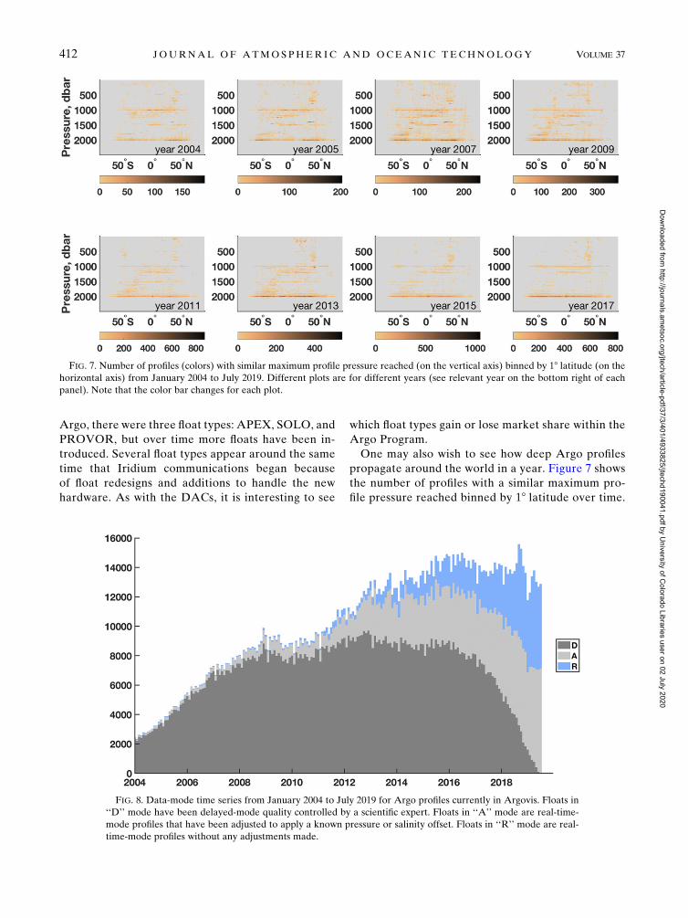
The history of data mode can easily be accessed also

(Fig. 8). A profile changes from ‘‘R’’ or ‘‘A’’ (real-time

mode), to ‘‘D’’ (delayed mode) after being quality

controlled by a scientific expert. This should happen

starting 12–18 months after the profile is measured.

Following this target, profiles older than 18 months

should be in ‘‘D’’ mode, but this is not yet the case for all

profiles (Fig. 8).

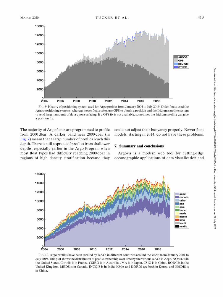
The history of the positioning system for profiles is

shown in Fig. 9. In the beginning of Argo, only the

Argos positioning system was used both to obtain the

position of floats and to transmit the data. Newer

floats are often deployed using the Iridium satellite

system instead, which allows two way communication

and faster transmission of larger quantities of data.

TABLE 2. Details for each API type. Boldface font indicates measured variables. Additional information may be found in the output of

Argovis API calls: this information is useful for the web application functioning but may not be useful for users.

API call types Input Output

Profile Platform no. and cycle no. lon, lat, position_qc,

POSITIONING_SYSTEM, date,

date_qc, date_added, cycle_number,

platform_number, PLATFORM_

TYPE, DATA_MODE, DATA_

CENTRE, station_parameters,

station_parameters_in_nc,

VERTICAL_SAMPLING_

SCHEME, DIRECTION, and

PI_NAME

Measurements: TEMP, PRES,

PSAL, and WMO_INST_TYPEPlatform Platform no.

Region Time range, pressure range,

set of lat and lon vertices

to define shape

Global metadata

by month

Month and year PRES_max_for_TEMP,

PRES_max_for_PSAL,

PRES_min_for_TEMP, andPRES_min_for_PSAL


Dow




https://argovis.colorado.edu/selection/profiles/10/2010/

https://argovis.colorado.edu/selection/profiles/10/2010/

The quality of the position fixes from Iridium is very

low, so GPS is usually used to determine the profile’s

position. If no GPS fix is available, the lower-quality

Iridium fix can be used instead. The number of Iridium

floats has been growing over time (Fig. 9), yet given

the 3–4-yr lifetime of a float, floats using the original

Argos system will still be producing profiles for sev-

eral years to come. In Fig. 9, the label ‘‘Other’’ in-

dicates profiles for which a typographical error is

detected in the transmission system key within the orig-

inal Argo netCDF file (and hence imported in Argovis).

The stack plot shown in Fig. 10 shows how many

profiles are produced by each data center (DAC) in

the Argovis database. The American DAC (AOML)

has always had the majority of files, but one can track

which DACs have grown or reduced in size over time.

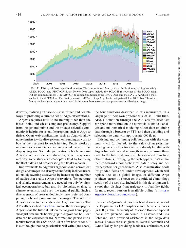
Users can also track the types of floats being used in

Argo over time as seen in Fig. 11. At the beginning of

FIG. 5. Labrador Sea (a),(b) bin-averaged temperature in time and (c),(d) number of

available observations in each bin. Bins are 10 dbar deep and include data for each month from

January 2004 to July 2019.

FIG. 6. Density of Argo profiles in 18 3 18 bins from January 2004 to July 2019. Only profiles

with position QC flag of 1 are included.


Dow




Argo, there were three float types: APEX, SOLO, and

PROVOR, but over time more floats have been in-

troduced. Several float types appear around the same

time that Iridium communications began because

of float redesigns and additions to handle the new

hardware. As with the DACs, it is interesting to see

which float types gain or lose market share within the

Argo Program.

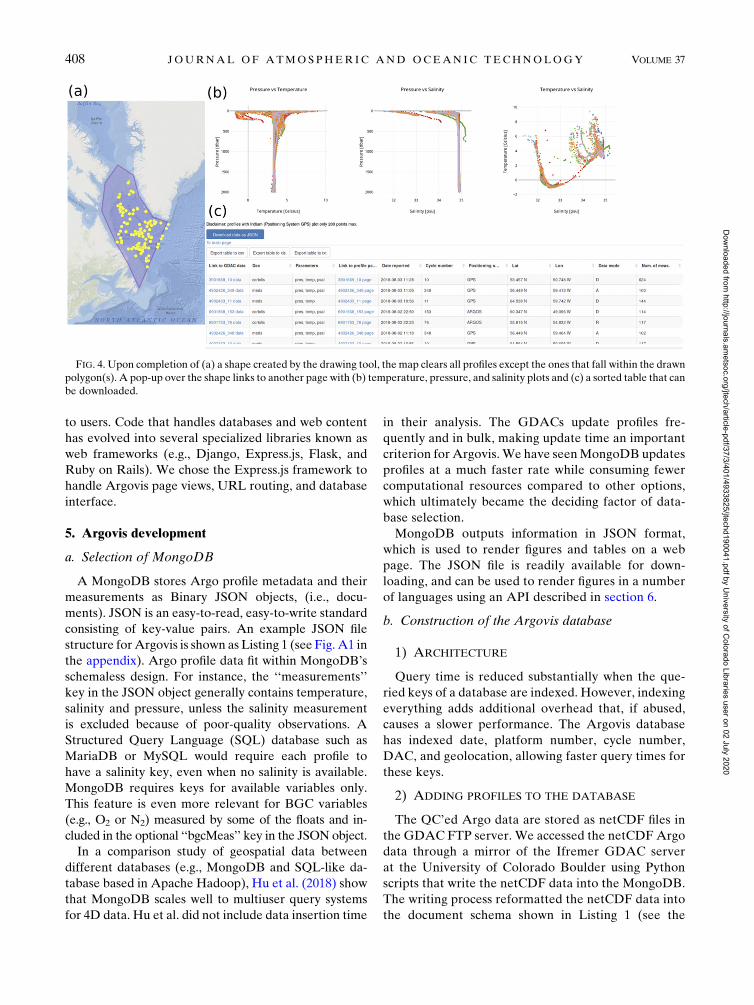
One may also wish to see how deep Argo profiles

propagate around the world in a year. Figure 7 shows

the number of profiles with a similar maximum pro-

file pressure reached binned by 18 latitude over time.

FIG. 7. Number of profiles (colors) with similar maximum profile pressure reached (on the vertical axis) binned by 18 latitude (on the

horizontal axis) from January 2004 to July 2019. Different plots are for different years (see relevant year on the bottom right of each

panel). Note that the color bar changes for each plot.

FIG. 8. Data-mode time series from January 2004 to July 2019 for Argo profiles currently in Argovis. Floats in

‘‘D’’ mode have been delayed-mode quality controlled by a scientific expert. Floats in ‘‘A’’ mode are real-time-

mode profiles that have been adjusted to apply a known pressure or salinity offset. Floats in ‘‘R’’ mode are real-

time-mode profiles without any adjustments made.


Dow




The majority of Argo floats are programmed to profile

from 2000 dbar. A darker band near 2000 dbar (in

Fig. 7) means that a large number of profiles reach this

depth. There is still a spread of profiles from shallower

depths, especially earlier in the Argo Program when

most float types had difficulty reaching 2000 dbar in

regions of high density stratification because they

could not adjust their buoyancy properly. Newer float

models, starting in 2014, do not have these problems.

7. Summary and conclusions

Argovis is a modern web tool for cutting-edge

oceanographic applications of data visualization and

FIG. 9. History of positioning system used for Argo profiles from January 2004 to July 2019. Older floats used the

Argos positioning systems, whereas newer floats often use GPS to obtain a position and the Iridium satellite system

to send larger amounts of data upon surfacing. If a GPS fix is not available, sometimes the Iridium satellite can give

a position fix.

FIG. 10. Argo profiles have been created by DACs in different countries around the world from January 2004 to

July 2019. This plot shows the distribution of profile ownership over time by the variousDACs inArgo.AOML is in

the United States. Coriolis is in France. CSIRO is in Australia. JMA is in Japan. CSIO is in China. BODC is in the

United Kingdom. MEDS is in Canada. INCOIS is in India. KMA and KORDI are both in Korea, and NMDIS is

in China.


Dow




delivery, featuring an ease-of-use interface and flexible

ways of providing a curated set of Argo observations.

Argovis requires little to no training other than the

basic ‘‘point and click’’ computer proficiency. Support

from the general public and the broader scientific com-

munity is helpful for scientific programs such as Argo to

thrive. Open web applications such as Argovis allow

nonscientists to visualize government funding at work to

bolster their support for such funding. Public kiosks at

museums or ocean science centers around the world can

display Argovis. Secondary-education schools may use

Argovis in their science education, which may even

motivate some students to ‘‘adopt’’ a float by following

the float’s data and broadcasting the float’s records.

Improvements to Argovis’s ergonomic and convenient

design encourages use also by scientifically inclined users,

ultimately favoring discoveries by increasing the number

of studies that analyze Argo observations. Temperature

and salinity measurements are needed not only by phys-

ical oceanographers, but also by biologists, engineers,

climate scientists, and even the general public. Such a

diverse group of users undoubtedly have preferred com-

puting tools and programming languages. The API for

Argovis tailors to the needs of the Argo community. The

API calls described in section 6 and on the tutorial page of

Argovis (via the tutorial link on the Argovis home page)

show just how simple hooking up toArgovis can be. Float

data can be extracted in JSON format and parsed into a

tabular format likeCSVorASCII in a few lines of code. It

is our thought that Argo scientists will write (and share)

the four functions described in this manuscript, in a

language of their own preference such as R and Julia.

Also, automation through the API ensures scientists

can spend more time on the nontrivial statistical anal-

ysis and mathematical modeling rather than obtaining

data through a browser or FTP, and then decoding and

selecting the data with appropriate QC flags.

Existing and continuing collaboration with the com-

munity will further add to the value of Argovis, im-

proving the work flow for scientists already familiar with

Argo observations and serving those not yet using these

data. In the future, Argovis will be extended to include

other datasets, leveraging the web application’s archi-

tecture toward a comprehensive data display and de-

livery system for geosciences. Also, visualization tools

for gridded fields are under development, which will

replace the static global images of different Argo

products currently shown on the gridded climatology

section of the website. Included in this development is

a tool that displays float trajectory probability fields.

Its most recent version is available online (at https://

argovis.colorado.edu/ng/covar).

Acknowledgments. Argovis is hosted on a server of

the Department of Atmospheric and Oceanic Sciences

(ATOC) at the University of Colorado Boulder. Special

thanks are given to Guilherme P. Castelao and Lisa

Lehmann, who provided assistance in the Argo data

access. Thanks are also given to Dean Roemmich and

Lynne Talley for providing feedback, enthusiasm, and

FIG. 11. History of float types used in Argo. There were fewer float types at the beginning of Argo—mainly

APEX, SOLO, and PROVOR floats. Newer float types include the SOLO-II (a redesign of the SOLO using

Iridium communications), the ARVOR (a compact redesign of the PROVOR), and the NAVIS-A, which is most

similar to the APEX float. The float types with ‘‘-D’’ are Deep Argo floats that go to 4000 or 6000 dbar. The other

float types have generally not been used in large numbers across several programs contributing to Argo.


Dow




https://argovis.colorado.edu/ng/covar

https://argovis.colorado.edu/ng/covar

encouragement. For his advice and guidance on imple-

menting the Angular web framework, we thank Julian

Pierret. This study was supported by the National Oceanic

and Atmospheric Administration Cooperative Science

Center for Earth System Sciences and Remote Sensing

Technologies (NOAA CREST) under the Cooperative

Agreement Grant NA16SEC4810008, Giglio’s research

funds provided by University of Colorado Boulder,

NSF EarthCube (Award 1928305), the U.S. NOAA

Cooperative Institute for Climate Science (Award

13342-Z7812001), the U.S. Argo Program through

NOAA Grant NA15OAR4320071 (CIMEC), and the

SOCCOM Project through Grant NSF PLR-1425989.

Tyler Tucker thanks the City College of New York,

NOAACRESTprogramandNOAAOffice ofEducation,

Educational Partnership Program for full fellowship

support at San Diego State University. Also he thanks

STATMOS (the Research Network for Statistical

Methods for Atmospheric and Oceanic Sciences) and

the U.S. National Science Foundation for travel sup-

port. The statements contained within this paper are

not the opinions of the funding agency or the U.S.

government but reflect only those of the authors. Argo

data are collected and made freely available by the

International Argo Program and the national programs

that contribute to it (http://www.argo.ucsd.edu; http://

argo.jcommops.org). The Argo dataset (http://doi.org/

10.17882/42182) used in this paper was downloaded from

the Ifremer GDAC (ftp://ftp.ifremer.fr/ifremer/argo).

APPENDIX

JSON Schema of MongoDB Profile

Listing 1 (Fig. A1) shows an example JSON file

structure for Argovis.

REFERENCES

Argo France, 2019: Argo active network map. Argo France, http://

www.argo-france.fr/en/welcome/.

Claustre, H., and Coauthors, 2010: Bio-optical profiling floats as

new observational tools for biogeochemical and ecosystem

studies: Potential synergies with ocean color remote sensing.

Proc. OceanObs’09: Sustained Ocean Observations and

Information for Society, Venice, Italy, ESA, https://doi.org/

10.5270/OceanObs09.cwp.17.

Gruber, N., and Coauthors, 2010: Adding oxygen to Argo:

Developing a global in situ observatory for ocean deoxygen-

ation and biogeochemistry. Proc. OceanObs’09: Sustained

Ocean Observations and Information for Society, Venice,

Italy, ESA, https://doi.org/10.5270/OceanObs09.cwp.39.

Hu, F., and Coauthors, 2018: Evaluating the open source data

containers for handling big geospatial raster data. ISPRS Int.

J. Geoinf., 7, 144, https://doi.org/10.3390/ijgi7040144.

JCOMMOPS, 2019: The WMO-IOC Joint Technical Commission

forOceanography andMarineMeteorology In SituObservations

Programme Support Centre. Argo France, http://argo.

jcommops.org.

Kuragano, T., Y. Fujii, and M. Kamachi, 2015: Evaluation of the

Argo network using statistical space-time scales derived from

satellite altimetry data. J. Geophys. Res. Oceans, 120, 4534–

4551, https://doi.org/10.1002/2015JC010730.

Kuusela, M., and M. L. Stein, 2018: Locally stationary spatio-

temporal interpolation of Argo profiling float data. Proc. Roy.

Soc., 474A, 20180400, https://doi.org/10.1098/RSPA.2018.0400.

FIG. A1. Listing 1: JSON schema of MongoDB profile.


Dow




http://www.argo.ucsd.edu



http://doi.org/10.17882/42182

http://doi.org/10.17882/42182

ftp://ftp.ifremer.fr/ifremer/argo

http://www.argo-france.fr/en/welcome/

http://www.argo-france.fr/en/welcome/

https://doi.org/10.5270/OceanObs09.cwp.17



https://doi.org/10.3390/ijgi7040144



https://doi.org/10.1002/2015JC010730

https://doi.org/10.1098/RSPA.2018.0400

Owens, W. B., and A. P. Wong, 2009: An improved calibration

method for the drift of the conductivity sensor on autonomous

CTD profiling floats by u–S climatology. Deep-Sea Res. I, 56,

450–457, https://doi.org/10.1016/j.dsr.2008.09.008.

Pierret, J., and S. S. P. Shen, 2017: 4D visual delivery of big cli-

mate data: A fast web database application system. Adv.

Data Sci. Adapt. Anal., 9, 1750006, https://doi.org/10.1142/

S2424922X17500061.

Roemmich, D., and J. Gilson, 2009: The 2004–2008 mean and an-

nual cycle of temperature, salinity, and steric height in the

global ocean from the Argo Program. Prog. Oceanogr., 82,

81–100, https://doi.org/10.1016/j.pocean.2009.03.004.

——, and Coauthors, 2009: The Argo Program: Observing the

global ocean with profiling floats. Oceanography, 22 (2), 34–

43, https://doi.org/10.5670/oceanog.2009.36.

Shen, S. S. P., G. P. Behm, Y. T. Song, and T. Qu, 2017: A dy-

namically consistent reconstruction of ocean temperature.

J. Atmos. Oceanic Technol., 34, 1061–1082, https://doi.org/

10.1175/JTECH-D-16-0133.1.

Smith, C. A., G. P. Compo, and D. K. Hooper, 2014: Web-Based

Reanalysis Intercomparison Tools (WRIT) for analysis and

comparison of reanalyses and other datasets. Bull. Amer.

Meteor. Soc., 95, 1671–1678, https://doi.org/10.1175/BAMS-D-

13-00192.1.


Dow




https://doi.org/10.1016/j.dsr.2008.09.008

https://doi.org/10.1142/S2424922X17500061

https://doi.org/10.1142/S2424922X17500061

https://doi.org/10.1016/j.pocean.2009.03.004

https://doi.org/10.5670/oceanog.2009.36

https://doi.org/10.1175/JTECH-D-16-0133.1

https://doi.org/10.1175/JTECH-D-16-0133.1

https://doi.org/10.1175/BAMS-D-13-00192.1

https://doi.org/10.1175/BAMS-D-13-00192.1

argovis: a web application for fast delivery

Documents