are power plant closures a breath of fresh air? local air
TRANSCRIPT

Are Power Plant Closures a Breath of Fresh Air?Local Air Quality and School Absences
Sarah Komisarow and Emily L. Pakhtigian∗
March 12, 2021
Abstract
In this paper we study the effects of three large, nearly-simultaneous coal-firedpower plant closures on school absences in Chicago. We find that the closures resultedin a 7 percent reduction in absenteeism in nearby schools relative to those farther awayfollowing the closures. For the typical elementary school in our sample, this trans-lates into around 372 fewer absence-days per year in the aggregate, or around 0.71fewer annual absences per student. We find that reductions in absences were larger inschools where pre-closure exposure to coal-fired power plants was more intense: namely,schools with low levels of air conditioning, schools more frequently in the wind pathof the plants, and non-magnet (i.e., neighborhood) schools where students were morelikely to live nearby. To explore potential mechanisms responsible for these absencereductions we investigate the effects of the closures on housing values and children’srespiratory health. We do not find statistical evidence of endogenous migration intoneighborhoods near the coal-fired power plants following the closures but do find de-clines in emergency department visits for asthma-related conditions among school-agechildren.
Keywords: Coal-fired power plants; Children; School absencesJEL codes: I10; I21; Q53
∗Komisarow (corresponding author): Sanford School of Public Policy, Duke University, Durham, NC27708 (email: [email protected]). Pakhtigian: School of Public Policy, Penn State University,University Park, PA 16802 (email: [email protected]).

1 Introduction
Despite dramatic declines in coal consumption and record numbers of coal-fired power plant
closures in the United States (U.S.), coal continues to account for nearly one-quarter of the
country’s electricity-generating fuel portfolio (MacIntyre and Jell, 2018; Mobilia and Com-
stock, 2019; Johnson and Chau, 2019; EIA, 2019). The burning of coal emits air pollution,
including pollutants such as sulfur dioxide (SO2), nitrogen oxides (NOx), and particulate
matter (PM). Although a growing literature in economics examines the effects of exposure
to these and other specific pollutants – either in isolation or simultaneously – on human
health and birth outcomes, little is known about the effects of the cumulative exposure to
coal-fired power plants on children.1
Exposure to coal-fired power plants may be more harmful to children’s health and well-
being than what previous evidence from the air pollution literature suggests for three reasons.
First, in addition to plant emissions, other activities surrounding coal-fired power plants
– including coal transport, storage, by-product, and disposal – negatively affect local air
quality (Jha and Muller, 2018; Zierold and Odoh, 2020). Second, coal-fired power plants are
known emitters of a host of pollutants – including mercury and other heavy metals – that
have been shown to negatively affect children’s health (Bose-O’Reilly et al., 2010) but that
are typically not measured in emissions inventories nor by air quality monitors. Omitted
measures of these pollutants could bias estimates of the effects of coal-fired power plants
that are solely based on measured pollutants, particularly if unmeasured pollutants have
different dispersion patterns or half-lives. Finally, children are potentially more vulnerable
to the negative effects of exposure to air pollution than are adults due to their (immature)
developmental status, breathing patterns, time spent outdoors, and time spent in activities
that raise ventilation (breathing) rates (Gauderman et al., 2004; Schwartz, 2004; Bateson
and Schwartz, 2007).
1We are aware of two studies that have examined the impacts of coal-fired power plant shut downs oninfant health. See Yang et al. (2017) and Yang and Chou (2018).
1

In this paper, we address this gap in the literature by estimating the effect of exposure
to coal-fired power plants on children in the short- and medium-run. We do this by exploit-
ing a unique and previously unexplored context: public elementary schools’ proximities to
operational coal-fired power plants. This context has the advantages of providing a setting
where children spend a substantial amount of time each day (second in terms of average
minutes only following time spent sleeping) (U.S. Environmental Protection Agency, 2008)
and in which a proxy for children’s health status is widely and uniformly measured among
the population of public school children (absences from school) (Weitzman, 1986; Currie
et al., 2009). This context also allows for in-depth examination of a potential mechanism –
school absences – that could help to explain existing evidence on the short-run effects of air
pollution exposure on student achievement and long-run effects on educational attainment
and earnings.2
We exploit variation induced by the closures of three large coal-fired power plants that
were located in, or in close proximity to, Chicago, Illinois. During a six-month period in
2012, the Crawford, Fisk Street, and State Line Generating Stations all closed abruptly after
decades of continuous operations. We use this natural experiment to estimate the effect
of exposure to coal-fired power plants on school absences using data from fifteen Illinois
school districts. This unique setting allows us to sharply identify short- and medium-term
impacts on children who attended schools near the three coal-fired power plants. This natural
experiment provides an ideal setting in which to study the effects of exposure to coal-fired
power plants on school absences because the power plant closures were unexpected, induced
large changes in local air quality, and had negligible impacts on employment in the Chicago
area.
Using difference-in-differences and event-study approaches, we find that school-level rates
of absences decreased by around 0.395 percentage points (7 percent) in schools located near
the plants (within 10 kilometers) following the closures. In more readily interpretable units,
2See for example, Ebenstein et al. (2016), Gilraine (2020), Sanders (2012), and Isen et al. (2017).
2
this reduction translates into around 372 fewer absence-days annually for the typical-sized
(median) treated elementary school in our sample, or around 0.71 fewer absence-days per
student per year. For several reasons we discuss later, we believe this estimate is likely
to be a lower bound of the effect. In addition to our results overall, we also investigate
effects on absences for student subgroups. We consistently find evidence to suggest that
absence reductions were larger for boys than for girls, which we believe to be consistent
with descriptive evidence on boys’ heightened underlying vulnerability (e.g., due to rates of
diagnosed asthma, activity patterns, etc.). We find weaker evidence to suggest that absence
reductions were larger for black students than for Hispanic students, although our estimates
for subgroups by race/ethnicity are less precise and more sensitive to model specification.
To provide evidence supporting the internal validity of our estimated effects on absences,
we investigate treatment heterogeneity based on the intensity of pre-closure exposure to coal-
fired power plants within our group of treated schools. Ex ante we expected larger effects
(in absolute terms) in schools where pre-closure exposure was higher (i.e., more intense). To
explore this, we partitioned our treatment group of schools using three distinct measures
to characterize “high” versus “low” exposure: wind intensity, air conditioning, and magnet
status. Our three separate approaches yielded a pattern of results that was remarkably con-
sistent: Reductions in absences were larger in schools with higher exposure. This exercise
lends credibility to our identification strategy by ruling out that the possibility that schools
near the plants were affected by unmeasured positive shocks to school quality, student en-
rollment, or other unobservables that improved student outcomes independently and that
were correlated with distance from the plants.
To gain insight into the specific mechanisms underlying our estimated effects on school
absences, we consider two possibilities suggested by previous literature: Endogenous migra-
tion of higher-income families to areas near the coal-fired power plants following their clo-
sures (mediated through housing prices) and improvements in children’s respiratory health.
We explore the possibility that higher-income (or otherwise socioeconomically advantaged)
3

families moved into neighborhoods near the coal-fired power plants following their closures
by examining housing values and the characteristics of students enrolled in nearby schools.
We also explore the effects of the closures on children’s respiratory health by examining
whether rates of emergency department visits for asthma-related conditions among school-
age children responded to the closures. We do not find any statistical evidence of endogenous
migration, but we do find large and meaningful reductions in emergency department visits
for asthma-related conditions among school-age children in areas near the three plants.
This paper contributes to the emerging literature on the effects of exposure to coal-fired
power plants and produces estimates that capture the full extent to which exposure to the
operations of coal-fired power plants affect children’s health. A final contribution of this
work is to examine the question of how exposure to coal-fired power plants affects children
in a setting that has historically been characterized by inequality. It is well-documented in
public health and environmental literatures that low-income and minoritized groups bear
disproportionate burdens of exposure to poor air quality in the U.S.3 We document that this
phenomenon extends to the locations of public schools. In 2016, approximately 2.3 million
elementary school children – in kindergarten through eighth grade – attended a public school
located within 10 kilometers of an operational coal-fired power plant (around 7 percent of the
public school population in this age range).4 Among these 2.3 million children, 81 percent
were eligible for free/reduced-price lunch, which is a proxy for low family income.5 The
context of our study, which we describe in more detail below, mirrors this national pattern.
Our paper sheds light on an important issue in a setting that disproportionately affects
children from disadvantaged backgrounds and, therefore, explores potential ways to reduce
entrenched inequality.
3Recent examples of this work include Colmer et al. (2020), Hausman and Stolper (2020), and Richmond-Bryant et al. (2020).
4See Appendix Figure A1.5Authors’ calculations. Please see Appendix B.
4

2 Background
2.1 Air Pollution, Children’s Health, and School Absences
Compared to adults, children are more susceptible to harm from exposure to air pollution
because of their unique and ongoing physical development and because of their activity pat-
terns. Children’s lungs and immune systems are less developed than adults’. This may
influence the penetration of fine particles within the lungs (when inhaled) and make them
more vulnerable to permanent damage (Bateson and Schwartz, 2007; World Health Organi-
zation, 2011). Aside from developmental differences, children also breathe differently than
adults, which increases their vulnerability. While adults commonly breathe through their
noses (nasal breathing), children often breathe through their mouths (oral breathing). Oral
breathing provides less air filtration and thus increases exposure, even when adults and chil-
dren are in the same ambient environment (Bateson and Schwartz, 2007; Foos et al., 2007).
Even conditional on nasal breathing – which increases as children age – children’s noses may
be less effective at air filtration due to differences in the anatomical structures of the nasal
passage (Foos et al., 2007). A final difference comes from potentially higher rates of depo-
sition of particles into the lower respiratory tract of the lungs, due to childhood conditions
such as obesity, hay fever (allergic rhinitis), and asthma (Foos et al., 2007).
Children’s activity patterns may also increase their exposure to air pollution. Children
spend more time outdoors than adults and more often participate in activities likely to
increase ventilation (breathing) rates. Both of these factors increase children’s exposure to
air pollution (Klepeis et al., 2001; Schwartz, 2004; Bateson and Schwartz, 2007). Among
children, time spent outdoors is highest among children ages 6-11, suggesting heightened
vulnerability of elementary school-age children relative to their older or younger peers (U.S.
Environmental Protection Agency, 2008).
Existing research on the effects of exposure to air pollution on school absences has ex-
amined the question in variety of settings and using different measures of exposure, thus
5

producing a wide range of estimates. Using changes in air quality resulting from a steel
mill shutdown, Ransom and Pope (1992) estimated that a 100 microgram per cubic meter
(µg/m3) increase in monthly average PM10 was associated with a 2 percentage point (40
percent) increase in rates of school absences. They further found that effects on absences
were larger for younger students relative to older students and that the effects persisted for
several weeks. Building on this work, Currie et al. (2009) developed a framework to consider
exposure to multiple pollutants including carbon monoxide (CO) and ozone (O3) in addition
to PM10. Using data from elementary and middle schools in thirty-nine school districts in
Texas, the authors found that for CO, one additional day of high exposure increased absences
by between 5 and 9 percentage points.
In recent work, Heissel et al. (2019) leveraged student school transitions to “upwind”
versus “downwind” schools near highways. They found that when students transitioned to a
downwind school, their absence rate increased by 0.5 percentage points (a 10 percent increase
relative to baseline), although this effect was only marginally statistically significant. Austin
et al. (2019) exploited variation in school bus retrofitting, which dramatically reduces diesel
emissions of nitrogen oxides (NOx) and fine particulates (PM2.5). They did not find any
statistically significant effects of retrofitting on attendance rates.
Two additional recent papers investigate the effect of exposure to particulate matter on
student absences in China, where air pollution levels are typically much higher than those
observed in the U.S. Chen et al. (2018) used an instrumental variables framework to assess
the effect of exposure to air pollution on absences in Guangzhou City. Using temperature
inversions as an instrument for air quality, the authors found that a one standard deviation
increase in daily Air Quality Index (AQI) levels lead to a 7 percent increase in absence rates.
Using information on reasons for absences, they found that absences on days with poor
air quality were mostly driven by increases in respiratory-related conditions, suggesting the
importance of short-run health channels. Consistent with this work, Liu and Salvo (2018)
found that increased exposure to PM2.5 led to increases in absences among students enrolled
6

in international schools in a major urban center in north China. They found that lagged daily
average PM2.5 levels in excess of 200 µg/m3 increased the likelihood of student absenteeism
by 0.9 percentage points (14 percent).
2.2 Coal-Fired Power Plant Closures and Changes in Air Quality
Between March and August of 2012, three large, coal-fired power plants located in (or on
the border of) Chicago, Illinois were unexpectedly closed, leading to significant changes in
local air quality. The Crawford and Fisk Street Generating Stations were located in Chicago
– on the south branch of the Chicago River – while the State Line Generating Station was
located in Hammond, Indiana, directly adjacent to the Illinois state (and Chicago city) line
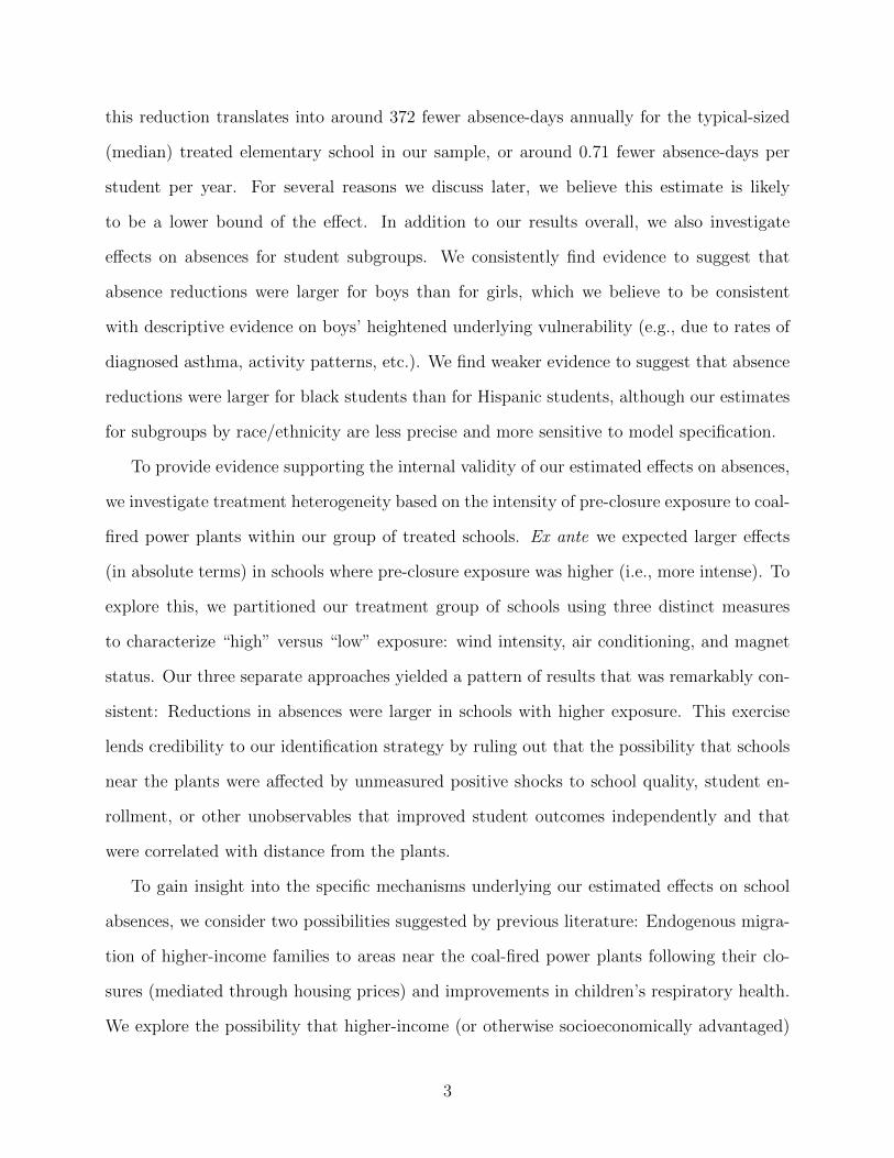
(Lydersen, 2012). The locations of the three coal-fired power plants are depicted in Figure
1.
In March 2012, the State Line Generating Station closed unexpectedly, in advance of a
previously announced closure date of 2014 (Tweh, 2010; Saltanovitz, 2011; Schneider Kirk,
2012). Six months later, in August 2012, the Crawford and Fisk Street Generating Stations
also closed unexpectedly and in advance of previously announced timelines. The parent
company cited an inability to make the financial investments necessary to upgrade pollution
control technologies and ongoing negotiations with environmental groups and state regulators
regarding the company’s portfolio of power plants across the state (Wernau, 2012b). In the
months leading up to their unexpected closures, all three plants were operating regularly.6
Further, at the time of the closures, the three coal-fired power plants collectively employed
around 280 workers, a negligible share of total employment in the Chicago metropolitan area
(Lydersen, 2012; Wernau, 2012c).
Prior to their closures, the Crawford, Fisk Street, and State Line Generating Stations
were among some of the largest operational coal-fired power plants in the U.S. The plants
were in the 70th (State Line), 69th (Crawford), and 59th (Fisk Street) percentiles of the coal-
6See Appendix Figure A2, in which we plot the time series of monthly capacity factors separately foreach plant between 2008-2012.
7
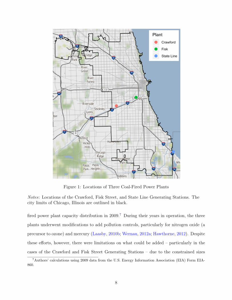
Figure 1: Locations of Three Coal-Fired Power Plants
Notes : Locations of the Crawford, Fisk Street, and State Line Generating Stations. Thecity limits of Chicago, Illinois are outlined in black.
fired power plant capacity distribution in 2009.7 During their years in operation, the three
plants underwent modifications to add pollution controls, particularly for nitrogen oxide (a
precursor to ozone) and mercury (Laasby, 2010b; Wernau, 2012a; Hawthorne, 2012). Despite
these efforts, however, there were limitations on what could be added – particularly in the
cases of the Crawford and Fisk Street Generating Stations – due to the constrained sizes
7Authors’ calculations using 2009 data from the U.S. Energy Information Association (EIA) Form EIA-860.
8

(and locations) of the plants’ physical sites (Wernau, 2012a). This meant that prior to their
closures, the three plants were among some of largest emitters of pollutants in the U.S.
(Laasby, 2010a; Hawthorne, 2010a; Wernau, 2011).8
Comparisons of air quality data in Chicago from the years before and after the three
coal-fired power plant closures reveal evidence of declines in concentrations of sulfur dioxide
(SO2), fine particulates (PM2.5), and Nitrogen Dioxide (NO2). In Figure 2 we plot annual
concentrations of SO2, PM2.5, and NO2 using averaged daily data from the air quality mon-
itoring station closest to each of the three plants (note: all three coal-fired power plants
operated for at least part of the year in 2012).9 Averaging the annual data in the years
before (2008-2011) and after the three coal-fired power plant closures (2013-2016) reveals
that SO2 declined by 4.09 parts per billion, PM2.5 declined by 2.29 µg/m3, and NO2 declined
by 5.64 parts per billion.
Although these changes cannot solely be attributed to the three coal-fired power plants,
the descriptive evidence does suggest that average air quality improved during the period
following their closures. The magnitudes of these estimates are in line with estimates reported
in previous literature on the topic of coal-fired power plant closures. Using data from 12
air quality monitoring stations in the Pittsburgh area (2500 square miles), Russell et al.
(2017) estimated PM2.5 reductions between 0.94-1.00 µg/m3. Jaffe and Reidmiller (2009)
estimated that a coal-fired power plant in the Columbia River Gorge contributed to annual
ambient concentrations of PM2.5 on the order of 0.90 µg/m3. Using a simple difference-
in-differences approach and studying the same three coal-fired power plants in Chicago,
Komisarow and Pakhtigian (2021) estimated that PM2.5 concentrations decreased by between
0.21-0.34 µg/m3 more in areas near the three coal-fired power plants relative to areas farther
8A federal lawsuit against Midwest Generation – the owner of the Crawford and Fisk Street Gener-ating Stations – accused the company of unfairly avoiding the installation of additional pollution controltechnologies on their plants (Hawthorne, 2005, 2007, 2010b).
9In some cases, a single station was the closest for two plants and in other cases there was no air qualitymonitoring station that was within 15 kilometers with consistent data for the entire period. See AppendixB for more detail on the air quality monitoring stations used for these calculations and their respectivedistances to each of the three coal-fired power plants.
9
(a) Sulfur Dioxide (SO2)
(b) Fine Particulates (PM2.5)
(c) Nitrogen Dioxide (NO2)
Figure 2: Average Annual Concentrations of Sulfur Dioxide, Fine Particulates, and NitrogenDioxide Based on Data from Air Quality Monitoring Stations Near the Crawford, Fisk Street,and State Line Generating Stations
Notes: The panels in this figure depict annual average concentrations of Sulfur Dioxide, Fine Particulates,and Nitrogen Dioxide using readings from the air quality monitoring stations closest to the Crawford, FiskStreet, and State Line Generating Stations. For more detail on the air quality monitoring stations andtheir distances to the coal-fired power plants, please see Appendix B.
10
away.
3 Data
3.1 School Data and Analytic Sample
We obtained information on school absences and other student characteristics aggregated at
the school-level for all public elementary schools (covering grades K-8) in Illinois from the
Illinois State Board of Education (ISBE) Report Card Data Library.10 Our primary outcome
in this paper is the annual aggregate absence rate at the school-level for students overall
and for student subgroups. From the ISBE Report Card Data Library we also obtained
the following time-varying school characteristics: total enrollment, percent black, percent
Hispanic, and percent low-income. From district webpages, we obtained information on two
time-varying policy controls relevant to public elementary schools in Chicago Public Schools
(CPS) – the largest district in our sample – during this period: Safe Passage Program status
(0/1) and Welcoming School status (0/1). These programs were introduced at a select
number of public elementary schools in CPS following the mass closings in CPS at the end
of the 2012/13 school year. For more information on the ISBE Report Card Data Library,
see Appendix B.
To define our sample and partition schools into treatment and control groups, we obtained
addresses for each traditional public elementary school in Illinois from annual published
versions of the state’s Directory of Educational Entities.11 We geocoded all addresses and
then merged these with school-level information from the ISBE Report Card Data Library.
We then calculated the linear distance between each school’s location and each of the three
10These data are publicly-available here: https://www.isbe.net/ilreportcarddata.11The Illinois Directory of Educational Entities is available here: https://www.isbe.net/Pages/
Data-Analysis-Directories.aspx. It contains information on all public entities that provide educationalservices to K-12 students in Illinois. The directory is updated continuously; snapshots are preserved eachschool year. The Illinois State Board of Education (ISBE) was unable to provide a snapshot for the 2015/16school year, however, so we imputed school addresses for this school year based on the address listed in theprevious school year.
11

power plants.
To define our analytic sample, we restricted our attention to the fifteen school districts in
Illinois that had at least one traditional public elementary school located within 10 kilometers
of at least one of the three coal-fired power plants. This resulted in a balanced panel of 457
traditional public elementary schools from fifteen school districts in Illinois (for a list of
districts, please see Appendix B). We dropped traditional public elementary schools that
changed locations at any point during the 2008/09-2015/16 school years, charter schools,
and any schools that newly opened or closed during this time period. Approximately 85
percent of the schools in our sample came from one school district: Chicago Public Schools
(CPS). CPS is the third largest school district in the U.S. and the single largest school
district in Illinois. CPS schools account for roughly 18 percent of schools and 25 of student
enrollment at the elementary school level in Illinois.12
3.2 Defining Treatment and Control Groups
In our main specifications, we defined schools as treated if they were located within 10
kilometers of at least one of the three coal-fired power plants; all other schools within the
fifteen districts were then designated as controls. All districts contained at least one treated
school and at least one control school. Although some papers in the air pollution literature
have selected smaller (1-mile) distance thresholds to partition treatment and control groups
(e.g., Currie et al. (2015) and Persico and Venator (2019)), these papers differ from ours
both in terms of the types of industrial facilities examined and the pollutants studied. Their
approaches to estimating the typical distance over which air pollution disperses relied on
data from thousands of industrial sources and hundreds of air quality monitoring stations
across much larger geographic areas (e.g., an entire state or multiple states). Given our
context, which relies on three coal-fired power plants and occurs in a setting with fewer than
20 air quality monitoring stations, we were unable to implement a similar approach.
12Authors’ calculations from the 2008/09 school year.
12
Instead, we chose a distance of 10 kilometers to divide treatment versus control schools
in our sample because it is the median distance in our fifteen district sample of elementary
schools. This distance likely underestimates the airborne distance that coal-fired power
plant emissions can travel. For example, in a recent paper examining the effects of exposure
to coal-fired power plants on birth outcomes, Yang and Chou (2018) find effects on birth
outcomes up to 60 miles away. We therefore acknowledge the possibility that students
attending schools in the control group were exposed to emissions from the three coal-fired
power plants–and, thus, to air quality improvements following their closures–and believe that
this potential control group contamination implies that our estimates should be interpreted
as lower bounds. We demonstrate later in the paper that our results are not sensitive to the
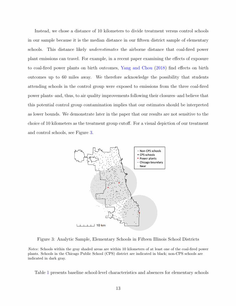
choice of 10 kilometers as the treatment group cutoff. For a visual depiction of our treatment
and control schools, see Figure 3.
Figure 3: Analytic Sample, Elementary Schools in Fifteen Illinois School Districts
Notes: Schools within the gray shaded areas are within 10 kilometers of at least one of the coal-fired powerplants. Schools in the Chicago Public School (CPS) district are indicated in black; non-CPS schools areindicated in dark gray.
Table 1 presents baseline school-level characteristics and absences for elementary schools
13

in our sample. Columns (1) and (2) present mean estimates and standard errors for the
457 elementary schools during the 2008/09 school year. Columns (2) and (3) present the
same descriptive information for our treatment (within 10 kilometers of at least one plant)
and control (more than 10 kilometers from all three plants) groups. Column (4) presents
the difference in means and associated standard errors, and Column (5) presents the p-value
from a two-tailed t-test of the difference in means.
Table 1: Descriptive Statistics, Elementary Schools in Fifteen Illinois School Districts,2008/09
(1) (2) (3) (4) (5)Full Sample Treatment Control Diff. p-value
Panel A. School Characteristics
Enrollment 608.16 593.19 645.81 -52.62 0.13(324.22) (318.79) (335.79) (34.32)
Percent Black 43.73 48.40 31.99 16.41*** 0.00(42.75) (43.39) (38.86) (4.17)
Percent Hispanic 39.08 40.36 35.86 4.50 0.19(37.49) (39.93) (30.39) (3.46)
Percent Low-Income 78.02 81.53 69.20 12.33*** 0.00(24.53) (22.14) (27.91) (2.74)
Panel B. Absence Rates5.53 5.81 4.82 0.99*** 0.00
All (1.90) (2.00) (1.40) (0.17)5.71 6.00 4.99 1.02*** 0.00
Male (2.03) (2.12) (1.56) (0.18)5.34 5.61 4.65 0.96*** 0.00
Female (1.82) (1.93) (1.29) (0.16)6.64 6.95 5.88 1.07*** 0.00
Black (2.37) (2.37) (2.19) (0.23)5.55 5.94 4.60 1.34*** 0.00
Hispanic (4.75) (5.37) (2.47) (0.38)5.66 5.90 5.04 0.86*** 0.00
Low-Income (1.85) (1.95) (1.39) (0.16)
Observations (Schools) 457 327 130
Notes: Column (1) reports means and standard deviations for the full sample of elementary schools from fifteen schoolsdistricts in Illinois. The fifteen districts included in the full sample are: Forest Park School District, Riverside School District,Oak Park Elementary School District, Berwyn North School District, Cicero School District, Berwyn South School District,Lyons School District, Summit School District, Central Stickney School District, Burbank School District, OakLawn-Hometown School District, Dolton School District, Burnham School District, Calumet City School District, and City ofChicago Public Schools. Column (2) reports means and standard deviations for schools within 10 kilometers (km) of at leastone of of the following three coal-fired power plants: Crawford Generating Station, Fisk Street Generating Station, and StateLine Generating Station. Column (3) reports means and standard deviations for schools located more than 10 kilometers (km)away from all three coal-fired power plants. Column (4) reports the difference in means (Near - Far) and the associatedstandard error. Column (5) reports the p-value from a two-tailed t-test of the difference in means. Asterisks indicatestatistical significance: * p <0.10, ** p < 0.05, ***p < 0.01.
14

At baseline, treatment group schools differed on numerous observable dimensions when
compared to schools in the control group. Prior to the coal-fired power plant closures,
treatment group elementary schools had higher percentages of black students (16 percentage
points) and higher percentages of low-income students (12 percentage points). We did not
find evidence of statistically significant differences in enrollment or the percentage of Hispanic
students enrolled in the school. We also find that treatment group schools had worse absence
outcomes at baseline (Panel (B)). This was true for students overall (0.60 percentage points
higher) and for all subgroups examined: male (1.02 percentage points higher), female (0.96
percentage points higher), black (1.07 percentage points higher), Hispanic (1.34 percentage
points higher), and low-income (0.86 percentage points higher).
4 Empirical Strategy
Due to the quasi-experimental nature of our context, we use difference-in-differences and
event-study approaches to estimate the effect of coal-fired power plant closures on student
absences. Both approaches exploit spatial variation in schools’ proximity to the Crawford,
Fisk Street, and State Line Generating Stations paired with temporal variation induced by
the nearly-simultaneous closures of the three plants.
4.1 Difference-in-Differences Specification
Our difference-in-differences approach assumes parallel trends in observable and unobservable
determinants of absences in our treatment and control groups in the years preceding the plant
closures. This assumption is required in order for the control group schools to provide a valid
counterfactual for how school-level absence outcomes in treated schools would have evolved
in the absence of the three plant closures. Even though this assumption is not explicitly
testable, we later provide evidence in support of the assumption and the validity of our
identification strategy.
15

We obtained difference-in-differences estimates using an equation of the following form:
Yst = α + β × (Near × Post)st + δt + φs +Xst · θ + εst (1)
Yst is a school-level absence outcome for school s in year t. (Near × Post)st is a binary
indicator that takes the value of one for all schools in the treatment group in school years
t = 2013, ..., 2016. We included a vector of year fixed-effects, δt, to control for factors that are
common across all elementary schools in the sample within specific school years, such as local
economic conditions, state-level school policy changes, and weather. We included a vector
of school fixed-effects, φs, to control for time-invariant school-level factors such as the local
environment, curricular differences, school policies, and neighborhood characteristics. Xst
is a vector of time-varying school characteristics and policy controls, including the natural
logarithm of total enrollment, the share of black students, the share of Hispanic students,
the share of low-income students, whether the school was designated as a Safe Passage
school (0/1), and whether the school was designated as a Welcoming School (0/1). We
report heteroskedasticity-robust standard errors clustered at the school level and weighted
all regressions by total enrollment to increase precision.
4.2 Event-Study Specification
To further investigate the validity of the parallel trends assumption and to explore dynamic
effects of the treatment, we modified our differences-in-differences specification by interacting
the indicator variable for schools in the treatment group, Nears, with event-time indicators.
This flexible approach allows for more detailed investigation of changes in school-level absence
outcomes around the year of the three plant closures. We present results based on estimating
the following equation:
Yst =4∑
j=−3j 6=−1
[πj ·Nears · 1 ·
(t− 2012 = j
)]+ φs + δt +Xst · θ + εst (2)
16

All components of Equation (2) are the same as the previous specification, although we
interacted Nears with event-time dummies. The sequence of πj coefficients for j = −3, ..., 4
(j = −1 omitted) traces out the evolution of relative differences in school-level absence rates
in treatment and control schools. In the plots we produce based on this equation, we set
j = 0 for the 2011/12 school year. Because the State Line Generating Station closed in
March 2012 – three months prior to the end of the 2011/12 school year, we consider this
school year to be “partially treated”. Elementary schools in the vicinity of the State Line
Generating Station experienced reduced exposure to coal-fired power plants for nearly one-
quarter of that school year. We thus expect coefficient estimates from π0 to be nonzero but
smaller in magnitude than those in the following school years, since only one of the three
plants had closed and for only part of the school year.
5 Main Results
5.1 Absences Overall and by Student Subgroup
Column (1) of Table 2 presents results for Equation (1) for absences among the full sample
of elementary schools. The point estimate indicates that aggregate absence rates were 0.395
percentage points lower in treatment schools relative to control schools in the years following
the three power plant closures. This reduction in absences represents a 7 percent decline
(baseline mean is 5.809 percent). For the typical (median) treated elementary school with
525 enrolled students, this absence rate decline represents a reduction of around 372 student-
absence days per year, or around 0.71 absences per student per year.13
Figure 4a depicts coefficients and associated ninety-five percent confidence intervals from
estimating Equation (2). Coefficient estimates corresponding to j = −3 and j = −2 depict
differences between the treatment and control groups in the years prior to the plant closures
compared to j = −1 (note: j = −1 is omitted). We cannot reject the null hypothesis that
13To covert the percentage point reduction in the aggregate absence rate at the school-level into absencesper student per year, we assume that all students were enrolled for the duration of the 180-day school year.
17

Table 2: Difference-in-Differences Estimates of the Effect of Power Plant Closures on Ab-sences, Overall and by Subgroup
All Male Female Black Hispanic Low-Income(1) (2) (3) (4) (5) (6)
Near X Post -0.395*** -0.440*** -0.349*** -0.431** -0.197** -0.337***(0.085) (0.088) (0.087) (0.183) (0.096) (0.094)
Baseline Mean 5.809 6.004 5.611 6.948 5.939 5.899
Observations 3656 3654 3654 3635 3493 3652
Notes: Each column reports results from a separate regression, where the dependent variable is aschool-level absence rate calculated among the full sample or student subgroup indicated in the columnheading. All regression specifications include school fixed-effects, year fixed-effects, total enrollment,percent black, percent Hispanic, percent low-income, Safe Passage (0/1), and Welcoming School (0/1). Allregressions are weighted by enrollment in the full sample or relevant subgroup. Heteroskedasticity-robuststandard errors are clustered at the school-level. Asterisks denote statistical significance: * p <0.10, **p < 0.05, ***p < 0.01.
both coefficients are jointly equal to zero (p = 0.76). This visual evidence suggests that
annual absence outcomes were trending similarly in treatment versus control schools prior
to the three coal-fired power plant closures. The coefficient estimate on j = 0 comes from
the 2011/12 school year, which we consider to be partially treated, due to the closure of the
State Line Generating Station prior to the end of the school year. The coefficient estimate
is negative but statistically indistinguishable from zero and is then followed by a sequence
of coefficients that become substantially more negative over time.
Columns (2)-(6) of Table 2 present results separately by student subgroup, including by
gender, race/ethnicity, and for low-income students. While we find suggestive evidence of
heterogeneous treatment effects by gender and by race/ethnicity, we we find that effects
for low-income students are very similar to our main effects for the full sample. This is not
surprising given that on average schools in our sample are comprised of 78 percent low-income
students. Columns (2) and (3) present results separately for absence rates among male and
female students. We consistently find that estimated effects on male students are larger
than effects on female students (the bootstrapped p-value on this difference is p = 0.038).
18

(a) All (b) Male
(c) Female (d) Black
(e) Hispanic (f) Low-Income
Figure 4: Event-Study Estimates, Absences
Notes: The panels in this figure depict event-study results for absences in fifteen Illinois school districts.Each plot depicts coefficient estimates from Equation (2) and their associated ninety-five percentconfidence intervals. t = 0 is the 2011/12 school year (partially treated) and t = −1 is omitted. Theevent-study specification includes school fixed-effects, year fixed-effects, the natural logarithm ofenrollment, percent black, percent Hispanic, percent low-income, Safe Passage (0/1), and WelcomingSchool (0/1). The regression is weighted by student enrollment. Heteroskedasticity-robust standard errorsare clustered at the school-level.
Aggregate absence rates were around 0.440 percentage points lower for males in treatment
schools versus control schools and 0.349 percentage points lower for female students in the
school years following the plant closures. In relative terms, these translate into 7 percent and
6 percent reductions. For the typical (median) treated elementary school with enrollment
19

split evenly between males and females, these declines represent reductions of 207 and 165
student-absence days per year, or around 0.79 and 0.63 fewer absences per student per year
among males and females, respectively. The visual evidence in Figures 4b and 4c are similar
to the results for the full sample, although once again effects are larger for males than for
females. This pattern of results is consistent with well-documented differences in asthma
prevalence and time use. Asthma prevalence is higher in boys than girls in this age range
(Akinbami et al., 2009), which suggests that boys are potentially more vulnerable to the
negative effects of exposure to coal-fired power plants compared to girls. This result is also
consistent with time-use patterns by gender in this age group: specifically, boys spend more
time outside than girls and more time engaged in moderate and vigorous physical activities,
which raises breathing rates (Nader et al., 2008; U.S. Environmental Protection Agency,
2008). These descriptive patterns also underscore boys’ heightened vulnerability relative to
girls’.
Columns (4) and (5) of Table 2 present results separately for black and Hispanic stu-
dents.14 These results reveal suggestive – albeit weaker – evidence of larger effects on black
students relative to Hispanic students. Aggregate absence rates were around 0.431 percent-
age points lower for black students in treatment schools versus control schools and 0.197
percentage points lower for Hispanic students in the years following the plant closures (the
bootstrapped p-value on this difference is p = 0.209). In relative terms, these translate into
7 percent and 3 percent reductions, respectively. The visual evidence in Figure 4d reveals a
pattern of effects on black students that are similar to the pattern observed in the full sample,
but the pattern of results for Hispanic students in Figure 4e is quite different. The effects
on Hispanic students are relatively constant in all of the years following the plant closures,
unlike the pattern of increasingly negative effects observed for all other groups. Column (6)
of Table 2 presents results for students from low-income families; Figure 4f depicts the event
study results. We find that the results are very similar to our results for the full sample
14We are unable to obtain results for other racial/ethnic groups due to high levels of non-reporting ofother subgroup absence rates at the school-level in our panel.
20

and believe that this is likely explained by the high percentage (78 percent) of low-income
students enrolled in the schools in our sample.
To assess the sensitivity of our estimates to the use of a 10-kilometer distance to define
the treatment group, we re-estimated our main model and allowed this distance to vary. We
plot the resulting coefficients and their associated ninety-five percent confidence intervals
for 1-kilometer increments ranging from 5 to 15 kilometers in Figure 5. In this figure, each
coefficient estimate comes from a separate regression in which we re-assigned schools to
treatment and control groups based on the distance indicated on the horizontal axis.
Our treatment effect estimate is slightly positive, though statistically insignificant, for a
distance of 5 kilometers, likely due to substantial control group contamination. The sequence
of estimates then crosses zero around 7 kilometers and becomes increasingly negative as we
allow the distance to increase. We note a “leveling-off” (i.e., flattening slope) between 10 and
11 kilometers, although in all cases the estimated effect continues to become more negative
past 10 kilometers – albeit only slightly. We interpret this as evidence that our choice of
10 kilometers is conservative (i.e., that some schools in our control group were affected by
the coal-fired power plant closures) and that our main results should be interpreted as lower
bounds on the treatment effect.
21

(a) All (b) Male
(c) Female (d) Black
(e) Hispanic (f) Low-Income
Figure 5: Estimated Treatment Effects Using Alternate Treatment Group Definitions (Dis-tance), Absences Overall and by Subgroup
Notes: This figure depicts estimated treatment effects for varying treatment group definitions (distance inkilometers). Each coefficient estimate comes from a separate regression in which the treatment group ofschools is defined based on the distance indicated on the horizontal axis; the control group of schools isthen comprised of all schools located farther than the specified distance (on the horizontal axis) from allthree coal-fired power plants.
In addition to our estimating equation outlined in Equation (1), we report estimates
using Equation (1) augmented with district-specific trends (Appendix Table A1) and from
unweighted regressions (Appendix Table A2), both of which are very similar to our main
results. We also report results from several falsification tests (Appendix Table A3) – using
22
outcomes related to school resources and instructional time that we expect to be unaffected
by coal-fired power plant closures. Our point estimates from these falsification tests are small
and statistically insignificant, and the associated ninety-five percent confidence intervals are
quite narrow. These results strengthen the causal interpretation of our absence results by
demonstrating that our estimates are not picking up the effects of unobserved improvements
in school resources or changes in teachers’ behavior that were correlated with the timing
of the closures or our choice of distance. Finally, we present two alternative approaches
to statistical inference, including standard errors clustered at the zip code-level (Appendix
Table A4) and non-parametric permutation tests (Appendix Table A5), which characterize
uncertainty in our estimates that arises from the assignment of schools to treatment and
control groups, rather than sampling. Our conclusions about the statistical significance of
our estimates remain unchanged.
5.2 Heterogeneous Effects by Pre-Closure Exposure Intensity
To provide evidence supporting the internal validity of our estimates, we investigated treat-
ment heterogeneity on the basis of the intensity of pre-closure exposure to coal-fired power
plants and their operations. We expected, ex ante, that the effects of the three coal-fired
power plant closures would be larger in treated schools where pre-closure exposure was more
intense. By partitioning schools within our treatment group on the basis of pre-closure ex-
posure intensity and by showing that exposure intensity is uncorrelated with distance, we
provide evidence that pre-closure exposure – and not unobservables correlated with distance
– is the main driver of our results. To investigate treatment heterogeneity along this dimen-
sion, we partitioned treated schools into two groups (i.e., “high” and“low” exposure) using
three characteristics: wind direction, air conditioning, and magnet status. We repeated this
exercise three times and report the results in Table 3.
As a first approach, we used daily wind data from the 2008/09 school year (baseline) to
split treatment group schools into two groups: “High Wind” and “Low Wind.” We created
23

Table 3: Heterogeneous Effects of Coal-Fired Power Plant Closures by Wind Intensity, AirConditioning, and School Magnet Status
All Male Female Black Hispanic Low-Income(1) (2) (3) (4) (5) (6)
Panel A. Days in Wind PathHigh Wind X Post -0.452*** -0.506*** -0.399*** -0.370* -0.370*** -0.385***
(0.095) (0.098) (0.098) (0.213) (0.100) (0.106)
Low Wind X Post -0.316*** -0.351*** -0.278*** -0.550** -0.037 -0.271**(0.105) (0.111) (0.106) (0.217) (0.105) (0.115)
p-value: Low vs. High Wind 0.221 0.184 0.282 0.392 0.000 0.343Baseline Mean 5.809 6.004 5.611 6.948 5.939 5.899Observations 3,656 3,654 3,654 3,635 3,493 3,652
Panel B. Air ConditioningLow AC X Post -0.518*** -0.604*** -0.439*** -0.466** -0.250* -0.501***
(0.134) (0.143) (0.132) (0.227) (0.137) (0.145)
High AC X Post -0.414*** -0.437*** -0.387*** -0.491** -0.187* -0.331***(0.102) (0.105) (0.105) (0.207) (0.105) (0.109)
p-value: Low vs. High AC 0.474 0.272 0.715 0.909 0.621 0.269Baseline Mean 5.809 6.004 5.611 6.948 5.939 5.899Observations 3,128 3,126 3,126 3,111 2,966 3,125
Panel C. School Magnet StatusNot Magnet X Post -0.427*** -0.463*** -0.380*** -0.652*** -0.217** -0.357***
(0.099) (0.104) (0.102) (0.221) (0.105) (0.110)
Magnet X Post -0.341*** -0.395*** -0.296*** -0.313 -0.186* -0.297***(0.103) (0.107) (0.105) (0.211) (0.107) (0.113)
p-value: Not Magnet vs. Magnet 0.449 0.566 0.462 0.112 0.736 0.626Baseline Mean 5.799 5.990 5.606 6.934 5.934 5.887Observations 3,624 3,622 3,622 3,604 3,462 3,620
Notes: Columns within panels report results from separate regressions, where the dependent variable is theaggregate absence rate calculated among the full sample or student subgroup indicated in the columnheading. All regression specifications include school fixed-effects, year fixed-effects, enrollment, percentblack, percent Hispanic, percent low-income, Safe Passage (0/1), and Welcoming School (0/1). Allregressions are weighted by student enrollment in the full sample or relevant subgroup. The control groupis comprised of schools located more than 10 kilometers away from all three coal-fired power plants.Heteroskedasticity-robust standard errors are clustered at the school-level. Asterisks denote statisticalsignificance: * p <0.10, ** p < 0.05, ***p < 0.01.
these two groups based the median number of days (45 days) during the school year on which
the school was directly in the wind path of the nearest plant (for a visual depiction, see
Appendix Figure A3).15 We then re-estimated Equation (1) with an interaction that allowed
15For more information on Wind Data sources, see Appendix B.
24
the treatment effect to vary between these two groups. We report results in Panel (A) of
Table 3. Our absence results in Columns (1)-(6) demonstrate that reductions in absence
rates were larger in High Wind compared to Low Wind schools, with the lone exception
appearing for black students in Column (4). Although we cannot reject the null hypothesis
of equal effects, the pattern is highly suggestive of larger effects in schools were pre-closure
exposure on the basis of wind was more intense.
As a second approach, we divided treated schools in our sample based on the percent
of the school building that was air-conditioned.16 The presence of air conditioning within
schools is likely to affect students’ exposure to coal-fired power plants in two ways: First,
schools with more air conditioning would be less likely to have open windows on hot days,
thus limiting the potential for outdoor air to circulate inside. Second, air conditioners (and
HVAC systems more generally) have basic air filtration capacities and thus provide some
filtering of outdoor air that circulates inside the school building (Parker et al., 2008). We
find evidence of the same pattern of exposure-based effect in Panel (B) of Table 3, where
the point estimates for schools with low levels of air conditioning are consistently larger in
magnitude than those for high levels of air conditioning. The lone exception is, once again,
for black students in Column (4).
As a final approach, we divided treated schools in our sample based on their magnet sta-
tus. We expect larger effects in non-magnet schools (i.e., schools with designated attendance
boundaries) since those schools draw from local neighborhoods and thus are more likely
to have students living nearby. If students’ residences were also more likely to be near the
plants, they would be exposed to coal-fired power plants not only at school but also at home.
Consistent with our previous findings, the estimates we report in Panel (C) of Table 3 once
again demonstrate a pattern of larger effects in high exposure (i.e., non-magnet) schools.
Our three approaches yielded results that were remarkably consistent with one another,
despite the fact that these school-level characteristics are essentially uncorrelated with one
16We obtained data on air conditioning in CPS schools from an Energy Star Audit in 2012. We wereunable to find data measuring this school-level characteristic from an earlier school year.
25

another, unrelated to the share of low-income students in the school, and uncorrelated with
school’s average distance from the three coal-fired power plants.17
5.3 Heterogeneous Effects by Dosage
Table 4 presents results from exercises designed to investigate the presence of heterogeneous
treatment effects by “dosage”. We measure dosage in three ways: close proximity to one
versus two coal-fired power plants, coal-fired power plant capacity, and distance.
Panel (A) reports results from the first exercise, in which we partitioned schools in the
treatment group into two groups: those located within 10 kilometers of one plant and those
located within 10 kilometers of two plants (there are no schools located within 10 kilometers
of all three coal-fired power plants). We find a pattern of results that is suggestive – albeit
somewhat weak – of a dose-response relationship. In all cases except one, the effect is larger
in magnitude for the group of schools located within 10 kilometers of two plants relative to
those located within 10 kilometers of just one. Although in most cases we cannot reject the
null hypothesis of equal effects, there one exception appears in Column (4), where we find
significant evidence of a stronger effect on absences for black students who attend schools
within 10 kilometers of two plants versus one.
As a second means to explore dosage effects, we assign treated schools to one of three
groups based on the nearest coal-fired power plant: Crawford, Fisk Street, or State Line.
Because the three coal-fired power plants had different capacities, we view this exercise as a
way to investigate whether the size of the plant influenced the magnitude of the treatment
effect.18 We do not find evidence of a monotonic relationship between plant size and the
magnitude of the treatment effect. Instead, we find a fairly consistent pattern of effects that
are largest at State Line, followed by Fisk, followed by Crawford, although this does not
hold for all subgroups and in most cases we cannot reject the null hypothesis that the effects
17For cross-sectional correlations between school-level air conditioning (percent), number of wind days,magnet status (0/1), and the percentage of low-income students in the school, see Appendix Table A6.
18State Line Generating Station was the largest (614 MWh), followed by Crawford (597 MWh), and Fisk(374 MWh).
26
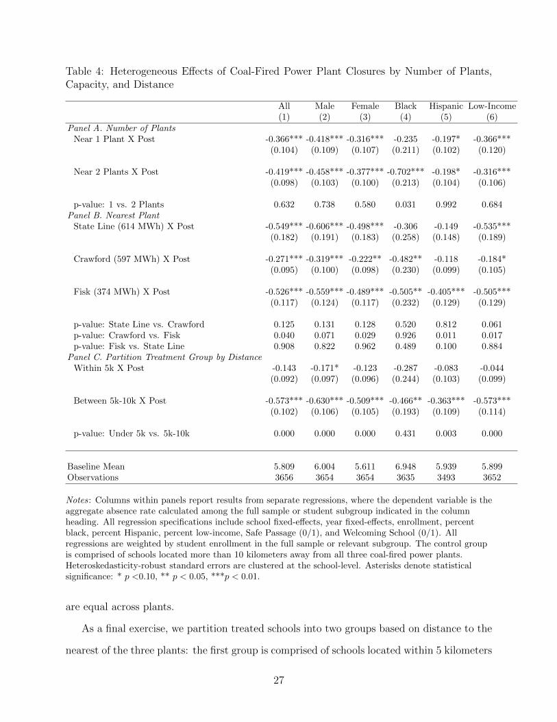
Table 4: Heterogeneous Effects of Coal-Fired Power Plant Closures by Number of Plants,Capacity, and Distance
All Male Female Black Hispanic Low-Income(1) (2) (3) (4) (5) (6)
Panel A. Number of PlantsNear 1 Plant X Post -0.366*** -0.418*** -0.316*** -0.235 -0.197* -0.366***
(0.104) (0.109) (0.107) (0.211) (0.102) (0.120)
Near 2 Plants X Post -0.419*** -0.458*** -0.377*** -0.702*** -0.198* -0.316***(0.098) (0.103) (0.100) (0.213) (0.104) (0.106)
p-value: 1 vs. 2 Plants 0.632 0.738 0.580 0.031 0.992 0.684Panel B. Nearest Plant
State Line (614 MWh) X Post -0.549*** -0.606*** -0.498*** -0.306 -0.149 -0.535***(0.182) (0.191) (0.183) (0.258) (0.148) (0.189)
Crawford (597 MWh) X Post -0.271*** -0.319*** -0.222** -0.482** -0.118 -0.184*(0.095) (0.100) (0.098) (0.230) (0.099) (0.105)
Fisk (374 MWh) X Post -0.526*** -0.559*** -0.489*** -0.505** -0.405*** -0.505***(0.117) (0.124) (0.117) (0.232) (0.129) (0.129)
p-value: State Line vs. Crawford 0.125 0.131 0.128 0.520 0.812 0.061p-value: Crawford vs. Fisk 0.040 0.071 0.029 0.926 0.011 0.017p-value: Fisk vs. State Line 0.908 0.822 0.962 0.489 0.100 0.884
Panel C. Partition Treatment Group by DistanceWithin 5k X Post -0.143 -0.171* -0.123 -0.287 -0.083 -0.044
(0.092) (0.097) (0.096) (0.244) (0.103) (0.099)
Between 5k-10k X Post -0.573*** -0.630*** -0.509*** -0.466** -0.363*** -0.573***(0.102) (0.106) (0.105) (0.193) (0.109) (0.114)
p-value: Under 5k vs. 5k-10k 0.000 0.000 0.000 0.431 0.003 0.000
Baseline Mean 5.809 6.004 5.611 6.948 5.939 5.899Observations 3656 3654 3654 3635 3493 3652
Notes: Columns within panels report results from separate regressions, where the dependent variable is theaggregate absence rate calculated among the full sample or student subgroup indicated in the columnheading. All regression specifications include school fixed-effects, year fixed-effects, enrollment, percentblack, percent Hispanic, percent low-income, Safe Passage (0/1), and Welcoming School (0/1). Allregressions are weighted by student enrollment in the full sample or relevant subgroup. The control groupis comprised of schools located more than 10 kilometers away from all three coal-fired power plants.Heteroskedasticity-robust standard errors are clustered at the school-level. Asterisks denote statisticalsignificance: * p <0.10, ** p < 0.05, ***p < 0.01.
are equal across plants.
As a final exercise, we partition treated schools into two groups based on distance to the
nearest of the three plants: the first group is comprised of schools located within 5 kilometers
27

of the nearest plant, while the second group is comprised of schools located between 5 and
10 kilometers of the nearest plant. We do not find any evidence of dosage effects based on
proximity; instead, we find robust evidence of larger effects on absences in schools located
between 5 and 10 kilometers from the nearest plant. We believe this is likely explained by
dispersion patterns that result from a combination of tall stacks and wind.19
6 Mechanisms
To examine the mechanisms underlying the reduced-form effects on absences presented in
the previous section, we consider two possibilities suggested by previous literature: endoge-
nous migration of higher-income families to neighborhoods near the plants following their
closures (mediated through housing price responses) and improvements in children’s respi-
ratory health. We first explore the possibility that the coal-fired power plant closures led to
endogenous migration; specifically, the sorting of higher-income or otherwise more socioeco-
nomically advantaged families into neighborhoods near the coal-fired power plants following
their closures. We do this by examining the effects of the closures on housing prices directly
and on the demographic composition of students enrolled in schools near the plants. We then
investigate the effects of the coal-fired power plant closures on children’s respiratory health
by examining whether emergency department visits for asthma-related conditions among
school-age children responded to the closures.
In Table 5 we present results from two sets of difference-in-differences regressions in which
we use housing values and rates of emergency department visits on the left-hand side. For
more detail about the housing value and emergency room visit data used in these analyses,
see Appendix B. In both cases, these data are aggregated up to the 5-digit zip code-level.
Our analysis follows Equation (1) as closely as possible; we consider zip codes to be treated
if their centroids fall within 10 kilometers of at least one of the three coal-fired power plants,
and control otherwise. Appendix Figure A4 depicts treatment and and control zip codes in
19Stack heights: Crawford (378 feet), Fisk Street (450 feet), and State Line (400 feet).
28
Chicago.
Previous empirical evidence on the responsiveness of housing values (prices) to toxic
plant operations comes from Currie et al. (2015), who find considerable asymmetry in price
responses to plant openings versus closures. Although Currie et al. (2015) find that toxic
plant openings lead to sizable declines in housing prices, their estimates indicate that plant
closures result in only small price increases (that are statistically insignificant) at best.20
Our findings, although somewhat less precise and covering a larger geographic area, are
consistent with the existing evidence. Our point estimates in Columns (1)-(3) of Panel (A)
suggest that – if anything – housing values in zip codes near the three coal-fired power plants
may have decreased slightly following the closures, although only one of the three estimates
is statistically significant. Consistent with previous work, we find no convincing evidence
that closures led to housing price increases. The upper bounds of the ninety-five percent
confidence intervals associated with our estimates are small enough to rule out housing value
increases larger than 3 percent. We present supporting event-study results for the same
dependent variable in Figure 6a. The lack of strong positive responses along this dimension
makes a story about the endogenous migration of higher-income families (mediated through
housing prices) unlikely. This evidence helps us rule out the story that our absence results
are driven by compositional changes of students (and families) within neighborhoods near
the coal-fired power plants.
To further investigate the issue of endogenous migration and compositional change, we
investigate the responses of enrollment levels and the demographic composition of students
who attended schools near the coal-fired power plants. Even in the absence of increases
in housing prices, it is still possible that high-income (or otherwise more socioeconomically
advantaged) families moved to the neighborhoods feeding into treatment group schools fol-
lowing the coal-fired power plant closures. If this were the case, this could help to explain
20“[P]lant closings appear to modestly increase housing prices, but this effect is small economically (lessthan 2 percent, even less than 0.5 miles from a plant) and statistically indistinguishable from zero” (Currieet al., 2015, p. 696).
29

Table 5: The Effect of Coal-Fired Power Plant Closures on Housing Prices and Rates ofEmergency Department Visits for Asthma-Related Conditions
(1) (2) (3) (4)Panel A. Log ZHVI
Near X Post -0.042 -0.032 -0.058** X(0.037) (0.030) (0.028) X
Baseline Mean 12.615Obs. 528 528 528
Panel B. Crude Rate of ED VisitsNear X Post -1.637** -1.676** -1.954* -2.145**
(0.691) (0.691) (1.103) (0.844)Baseline Mean 21.241Obs. 384 384 384 288
Year and Zip FE X X X XCovariates X X XZip Code Trends XTruncated Sample X
Notes: Each cells reports results from a separate regression, where the dependent variable is the naturallogarithm of zip code-level housing values (Panel A) or the crude rate of emergency department visits forasthma-related conditions among school-age children (Panel B). All regressions are weighted by zip codepopulation. Heteroskedasticity-robust standard errors are clustered at the zip code-level. Asterisks denotestatistical significance: * p <0.10, ** p < 0.05, ***p < 0.01.
our absence-related findings because high-income students are less likely to be absent – on
average – than low-income students (Gershenson et al., 2016). We do not find any statis-
tically significant effects of the coal-fired power plant closures on the natural logarithm of
enrollment nor on the percentages of black, Hispanic, or low-income students enrolled in the
school. All of the point estimates are small, and the associated ninety-five percent confidence
intervals are narrow. We report these results in Appendix Table A7.
To probe whether decreases in absences were generated through improvements in chil-
dren’s respiratory health, we present results from a series of regressions that investigate the
effects of the three coal-fired power plant closures on rates of emergency department visits
for asthma-related conditions among school-age children.21 This outcome measure captures
more extreme health-driven responses to the coal-fired power plant closures than school ab-
sences themselves. Columns (1)-(4) of Panel (B) present our results for the crude rate of
21We define school-age children as those between the ages of 5 and 18. For more information on thediagnoses included in the definition of asthma-related conditions, please see Appendix B.
30

(a) Housing Values (Natural Log of ZHVI)
(b) Rate of ED Visits for Asthma-RelatedConditions Among 5-18 Year-Olds
Figure 6: Event-Study Estimates for Housing Prices and Rates of Emergency DepartmentVisits for Asthma-Related Conditions
Notes: This figure depicts event-study results for housing values and rates of emergency department (ED)visits for asthma-related conditions among 5-18 year olds. The plots depict coefficient estimates and theirassociated ninety-five percent confidence intervals (note: 2011 is omitted). The event-study specificationincludes zip code fixed-effects, year fixed-effects, and all regressions are weighted by zip code population.Emergency department visit rate data are missing for 2015. Heteroskedasticity-robust standard errors areclustered at the zip-code level.
emergency department visits for asthma-related conditions among school-age children.22 We
find that emergency department visits decreased in treatment group zip codes by around 1.64
visits per ten thousand residents per year (7 percent) following the three coal-fired power
plant closures. This result is robust to the inclusion of time-varying covariates (Column
(2)), zip-code specific linear trends (Column (3)), and truncation of the sample after 2014
(Column (4)), which is a check to ensure that our results are not driven by a change in the
22The crude rate measures the number of emergency department visits for asthma-related conditionsamong school-age children per ten thousand residents in the zip code.
31

coding of asthma-related conditions that occurred in 2015 (for more information, see Ap-
pendix B). We present supporting event-study results in Figure 6b. As a robustness check,
we present the same regression and event-study results for age-specific rates of emergency
department visits in Appendix Table A8 and Appendix Figure A5. These results are very
similar to our main results using the crude rate and provide reassurance that our findings
are not driven by changes in population (the denominator of our outcome variable) in other
age ranges. Interpreted in light of existing medical evidence on children’s vulnerability to air
pollution exposure (Schwartz, 2004; Bateson and Schwartz, 2007), we believe that this evi-
dence supports improvements in children’s respiratory health as a primary channel through
which coal-fired power plant closures improved school attendance.
7 Conclusion
In this paper we estimate the causal effect of three, nearly-simultaneous coal-fired power
plant closures on school absences. We exploit quasi-experimental variation in exposure to
coal-fired power plants induced by the closures to estimate the effect of exposure on children’s
health. This unique context – in which large industrial sources abruptly closed after decades
of operation – allows us to sharply identify short-run and medium-run effects. We find
that school-level absence rates decreased by around 0.395 percentage points (7 percent) in
schools located near the plants following their closures. This translates into 372 fewer student
absence-days per year for the typical elementary school, or around 0.71 fewer absence-days
per student per year. In addition to our results overall, we also investigate effects on absences
for student subgroups. We consistently find evidence to suggest that absence reductions were
larger for boys than for girls. We also find evidence – albeit much weaker – to suggest that
absence reductions were larger for black students than for Hispanic students.
We investigate the possibility of heterogeneous treatment effects on the basis of exposure
intensity as a means to assess the internal validity of our main results. By examining
heterogeneity within our treatment group, we rule out the possibility that our results are
32

driven by unobserved shocks correlated with distance and the timing of the three coal-fired
power plant closures. Our three approaches – using data on windy days, air conditioning,
and magnet schools – yield a consistent pattern of results: reductions in absences were larger
in schools with higher baseline exposure to emissions from coal-fired power plants.
Finally, we gain insight into the mechanisms underlying our estimated effects on school
absences by exploring the effects of coal-fired power plant closures on housing prices (and
the composition of schools near the plants) and children’s respiratory health. We do not
find consistent statistical evidence to suggest that the three coal-fired power plant closures
affected housing prices – if anything, we find some weak evidence to suggest that housing
prices actually declined slightly in zip codes near the three plants following their closures.
We do not find any statistically significant effects of the three coal-fired power plant closures
on school enrollments nor on the demographic composition of students in schools near the
plants. We do, however, find evidence to suggest that children’s respiratory health improved
following the three coal-fired power plant closures. Specifically, we find that rates of emer-
gency department visits for asthma-related conditions declined among school-age children in
zip codes near the plants compared to zip codes farther away. When considered together,
these results from these exercises strongly suggest improved respiratory health as a primary
absence-reducing channel.
This paper contributes to the emerging literature on the effects of exposure to coal-fired
power plants on human health and to the larger literature on the effects of air pollution
exposure on children’s outcomes more broadly. The results from this work contribute to
understanding how current trends in energy generation in the U.S. – away from coal –
may have broad and far-reaching impacts. In so doing, we provide insight into how the
ongoing energy transition in the U.S. and in other countries experiencing such changes could
benefit (or harm, in the case of increased coal use) children who live and attend school near
coal-fired power plants. Given the geographical distribution of operational coal-fired power
plants – and other large, industrial pollution emitters – our findings suggest that current
33

trends in energy generation and transitions toward alternative sources of energy could also
be influential in reducing inequality.
34

References
Akinbami, L. J., Moorman, J. E., Garbe, P. L., and Sondik, E. J. (2009). Status of ChildhoodAsthma in the United States, 1980–2007. Pediatrics, 123(Supplement 3):S131–S145.
Austin, W., Heutel, G., and Kreisman, D. (2019). School bus emissions, student health andacademic performance. Economics of Education Review, 70:109–126.
Bateson, T. F. and Schwartz, J. (2007). Children’s Response to Air Pollutants. Journal ofToxicology and Environmental Health, Part A, 71(3):238–243.
Bose-O’Reilly, S., McCarty, K. M., Steckling, N., and Lettmeier, B. (2010). Mercury Expo-sure and Children’s Health. Current Problems in Pediatric and Adolescent Health Care,40(8):186–215.
Chen, S., Guo, C., and Huang, X. (2018). Air Pollution, Student Health, and School Ab-sences: Evidence from China. Journal of Environmental Economics and Management,92:465–497.
Colmer, J., Hardman, I., Shimshack, J., and Voorheis, J. (2020). Disparities in PM2.5air pollution in the United States. Science, 369(6503):575–578. Publisher: AmericanAssociation for the Advancement of Science Section: Report.
Currie, J., Davis, L., Greenstone, M., and Walker, R. (2015). Environmental Health Risksand Housing Values: Evidence from 1,600 Toxic Plant Openings and Closings. AmericanEconomic Review, 105(2):678–709.
Currie, J., Hanushek, E. A., Kahn, E. M., Neidell, M., and Rivkin, S. G. (2009). DoesPollution Increase School Absences? Review of Economics and Statistics, 91(4):682–694.
Ebenstein, A., Lavy, V., and Roth, S. (2016). The Long-Run Economic Consequences ofHigh-Stakes Examinations: Evidence from Transitory Variation in Pollution. AmericanEconomic Journal: Applied Economics, 8(4):36–65.
EIA, U. (2019). Frequently Asked Questions (FAQs) - U.S. Energy Information Administra-tion (EIA).
Foos, B., Marty, M., Schwartz, J., Bennett, W., Moya, J., Jarabek, A. M., and Salmon,A. G. (2007). Focusing on Children’s Inhalation Dosimetry and Health Effects for RiskAssessment: An Introduction. Journal of Toxicology and Environmental Health, Part A,71(3):149–165.
Gauderman, W. J., Avol, E., Gilliland, F., Vora, H., Thomas, D., Berhane, K., McConnell,R., Kuenzli, N., Lurmann, F., Rappaport, E., Margolis, H., Bates, D., and Peters, J.(2004). The Effect of Air Pollution on Lung Development from 10 to 18 Years of Age.New England Journal of Medicine, 351(11):1057–1067.
Gershenson, S., Jacknowitz, A., and Brannegan, A. (2016). Are Student Absences Worth theWorry in U.S. Primary Schools? Education Finance and Policy, 12(2):137–165. Publisher:MIT Press.
35

Gilraine, M. (2020). Air Filters, Pollution and Student Achievement. Technical report,Annenberg Institute at Brown University. Publication Title: EdWorkingPapers.com.
Hausman, C. and Stolper, S. (2020). Inequality, Information Failures, and Air Pollution.Technical Report w26682, National Bureau of Economic Research.
Hawthorne, M. (2005). Madigan Says EPA Goes Easy on Coal Plants. Chicago Tribune.
Hawthorne, M. (2007). EPA Cites Coal Plants; Utility’s 6 Illinois Sites Release Too MuchSoot, U.S. says. Chicago Tribune.
Hawthorne, M. (2010a). Dirty Truth Next Door: Utility Says Plant Will Keep Running –And Polluting – Until Forced to Close. Chicago Tribune; Chicago, Ill., page 1.1.
Hawthorne, M. (2010b). EPA Targets Coal-Fired Power Plants: New Rule Would Cut Smog,Soot Here, Across U.S. Chicago Tribune.
Hawthorne, M. (2012). 2 Coal-Burning Plants to Power Down Early. Chicago Tribune.
Heissel, J., Persico, C., and Simon, D. (2019). Does Pollution Drive Achievement? TheEffect of Traffic Pollution on Academic Performance. Technical Report w25489, NationalBureau of Economic Research, Cambridge, MA.
Isen, A., Rossin-Slater, M., and Walker, W. R. (2017). Every Breath You Take—EveryDollar You’ll Make: The Long-Term Consequences of the Clean Air Act of 1970. Journalof Political Economy, 125(3):848–902.
Jaffe, D. A. and Reidmiller, D. R. (2009). Now you see it, now you don’t: Impact oftemporary closures of a coal-fired power plant on air quality in the Columbia River GorgeNational Scenic Area. Atmos. Chem. Phys., 9:7997–8005.
Jha, A. and Muller, N. Z. (2018). The Local Air Pollution Cost of Coal Storage and Handling:Evidence from U.S. Power Plants. Journal of Environmental Economics and Management,92:360–396.
Johnson, S. and Chau, K. (2019). More U.S. Coal-Fired Power Plants Are Decommissioningas Retirements Continue. Today in Energy, U.S. Energy Information Administration.
Klepeis, N. E., Nelson, W. C., Ott, W. R., Robinson, J. P., Tsang, A. M., Switzer, P., Behar,J. V., Hern, S. C., and Engelmann, W. H. (2001). The National Human Activity Pat-tern Survey (NHAPS): A Resource for Assessing Exposure to Environmental Pollutants.Journal of Exposure Science & Environmental Epidemiology, 11(3):231.
Komisarow, S. and Pakhtigian, E. L. (2021). The Effect of Coal-Fired Power Plant Closureson Emergency Department Visits for Asthma-Related Conditions Among 0-4 Year-OldChildren in Chicago, 2009-2017. American Journal of Public Health, Forthcoming.
Laasby, G. (2010a). Dominion Will Shut Down State Line Power Plant. The Post-Tribune,page 5.
36

Laasby, G. (2010b). Plant’s Smoke A Bad Habit. The Post-Tribune, page 2.
Liu, H. and Salvo, A. (2018). Severe Air Pollution and Child Absences When Schools andParents Respond. Journal of Environmental Economics and Management, 92:300–330.
Lydersen, K. (2012). Closing of State Line Power Station, on Illinois-Indiana Border, IsExpected to Leave Problems Behind. The New York Times.
MacIntyre, S. and Jell, S. (2018). U.S. Coal Consumption in 2018 Expected To Be theLowest in 39 Years. Today in Energy, U.S. Energy Information Administration.
Mobilia, M. and Comstock, O. (2019). Petroleum, Natural Gas, and Coal Continue toDominate U.S. Energy Consumption. Today in Energy, U.S. Energy Information Admin-istration.
Nader, P. R., Bradley, R. H., Houts, R. M., McRitchie, S. L., and O’Brien, M. (2008).Moderate-to-Vigorous Physical Activity From Ages 9 to 15 Years. JAMA, 300(3):295–305. Publisher: American Medical Association.
Parker, J. L., Larson, R. R., Eskelson, E., Wood, E. M., and Veranth, J. M. (2008). Particlesize distribution and composition in a mechanically ventilated school building during airpollution episodes. Indoor Air, 18(5):386–393.
Persico, C. L. and Venator, J. (2019). The Effects of Local Industrial Pollution on Studentsand Schools. Journal of Human Resources, pages 0518–9511R2. Publisher: University ofWisconsin Press.
Ransom, M. R. and Pope, C. A. (1992). Elementary School Absences and PM10 Pollutionin Utah Valley. Environmental Research, 58(1):204–219.
Richmond-Bryant, J., Mikati, I., Benson, A. F., Luben, T. J., and Sacks, J. D. (2020).Disparities in Distribution of Particulate Matter Emissions from US Coal-Fired PowerPlants by Race and Poverty Status After Accounting for Reductions in Operations Between2015 and 2017. American Journal of Public Health, 110(5):655–661. Num Pages: 655-661Place: Washington, United States Publisher: American Public Health Association Section:CLIMATE CHANGE.
Russell, M. C., Belle, J. H., and Liu, Y. (2017). The impact of three recent coal-firedpower plant closings on Pittsburgh air quality: A natural experiment. Journal of theAir & Waste Management Association, 67(1):3–16. Publisher: Taylor & Francis eprint:https://doi.org/10.1080/10962247.2016.1170738.
Saltanovitz, M. (2011). State Line Power Plant to Close at End of 2012. The Times.
Sanders, N. J. (2012). What Doesn’t Kill You Makes You Weaker: Prenatal PollutionExposure and Educational Outcomes. Journal of Human Resources, 47(3):826–850.
Schneider Kirk, C. (2012). State Line Energy Exhausts Coal Supply, Focus Turns to Cleanup.The Times.
37

Schwartz, J. (2004). Air Pollution and Children’s Health. Pediatrics, 113(4):1037–1043.
Tweh, B. (2010). Exec: State Line Power Plant Could Close in 2014. The Times.
U.S. Environmental Protection Agency (2008). Child-Specific Exposure Factors Handbook.EPA/600/R-06/096F, National Center for Environmental Assessment, Office of Researchand Development, Washington, DC.
Weitzman, M. (1986). School absence rates as outcome measures in studies of children withchronic illness. Journal of Chronic Diseases, 39(10):799–808.
Wernau, J. (2011). Coal Is Getting Cleaner, But Consumers Will Foot the Bill: New Envi-ronmental Regulations Mean Power Plants Must Retrofit Or Rebuild. Chicago Tribune.
Wernau, J. (2012a). Clean Is In the Air: Battle to Close Coal Plants Is a Lesson in Historyand Politics. Chicago Tribune.
Wernau, J. (2012b). Closure of Chicago’s Crawford, Fisk Electric Plants Ends Coal Era.Chicago Tribune.
Wernau, J. (2012c). Midwest Generation to Close 2 Chicago Coal Plants Early. ChicagoTribune.
World Health Organization (2011). Summary of Principles for Evaluating Health Risksin Children Associated with Exposure to Chemicals. Technical report, World HealthOrganization, Geneva, Switzerland.
Yang, M., Bhatta, R. A., Chou, S.-Y., and Hsieh, C.-I. (2017). The Impact of PrenatalExposure to Power Plant Emissions on Birth Weight: Evidence from a PennsylvaniaPower Plant Located Upwind of New Jersey. Journal of Policy Analysis and Management,36(3):557–583. eprint: https://onlinelibrary.wiley.com/doi/pdf/10.1002/pam.21989.
Yang, M. and Chou, S.-Y. (2018). The impact of environmental regulation on fetal health:Evidence from the shutdown of a coal-fired power plant located upwind of New Jersey.Journal of Environmental Economics and Management, 90:269–293.
Zierold, K. M. and Odoh, C. (2020). A review on fly ash from coal-fired power plants:chemical composition, regulations, and health evidence. Reviews on Environmental Health,35(4):401–418. Publisher: De Gruyter Section: Reviews on Environmental Health.
38

Appendix A: Supplemental Results
Figure A1: Coal-Fired Power Plant Locations and K-8 Public School Enrollment in theUnited States, 2016
Notes: This figure depicts the locations of operational coal-fired power plants in the United States in 2016.Dot sizes represent the number of K-8 students enrolled in a public school located within 10 kilometers(km) of the plant. Power plants depicted in red have public schools (K-8) within 10 km of their operation;power plants depicted in blue do not. Power plant locations, energy sources, and operational status comefrom the United States Energy Information Administration (EIA) Form EIA-860. Public school locationsand enrollments come from the Elementary and Secondary Information System (ElSi) of the NationalCenter for Education Statistics (NCES) of the United States Department of Education.
39
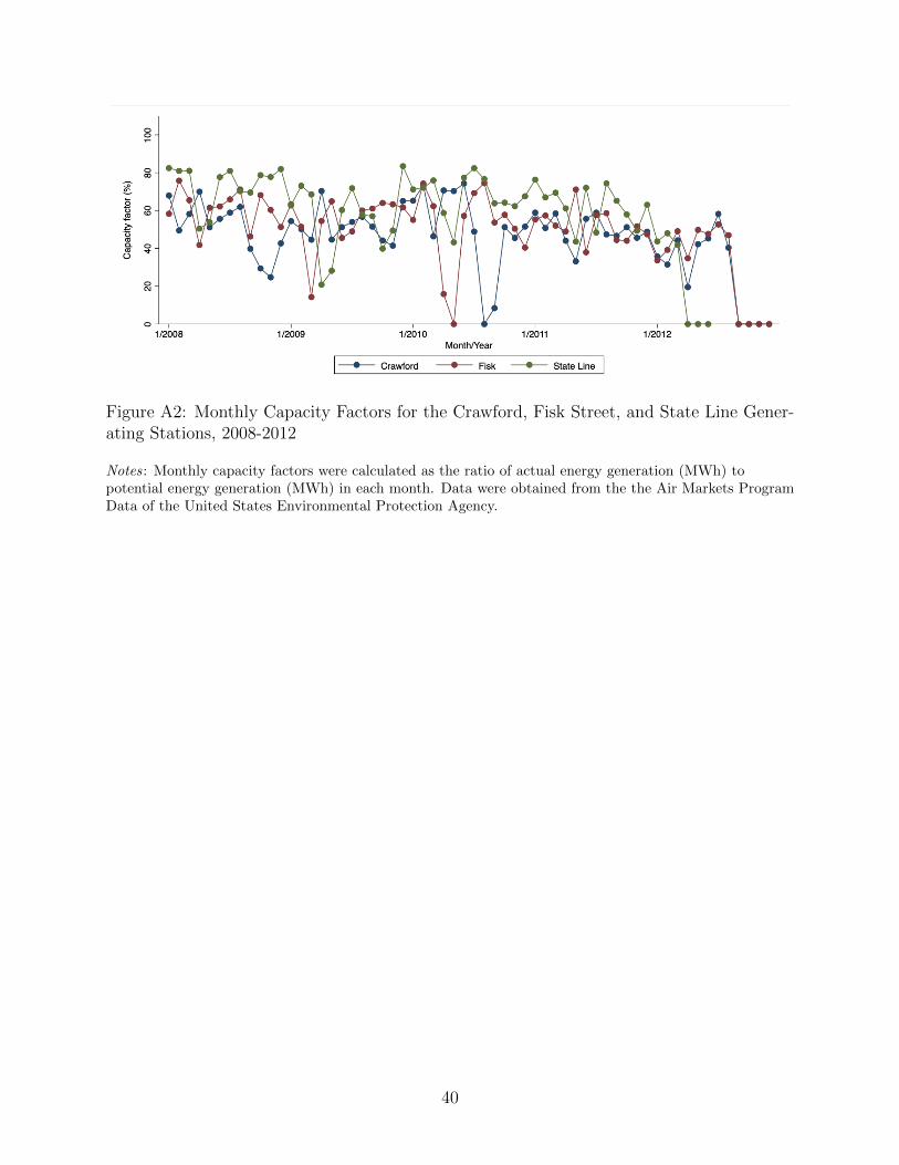
Figure A2: Monthly Capacity Factors for the Crawford, Fisk Street, and State Line Gener-ating Stations, 2008-2012
Notes: Monthly capacity factors were calculated as the ratio of actual energy generation (MWh) topotential energy generation (MWh) in each month. Data were obtained from the the Air Markets ProgramData of the United States Environmental Protection Agency.
40

(a) School in Wind Path
(b) School Not in Wind Path
Figure A3: School in Wind Path versus Not in Wind Path
Notes: This figure illustrates how we classified High versus Low Wind school days. The blue arrow depictsthe direction from which the day’s wind originated.
41

Figure A4: Map of Treatment and Control Zip Codes
Notes: This figure shows the zip codes designated as treatment (shaded in gray) and control (in white) inthe analysis of housing values and emergency department visits for asthma-related conditions amongschool-age children.
42
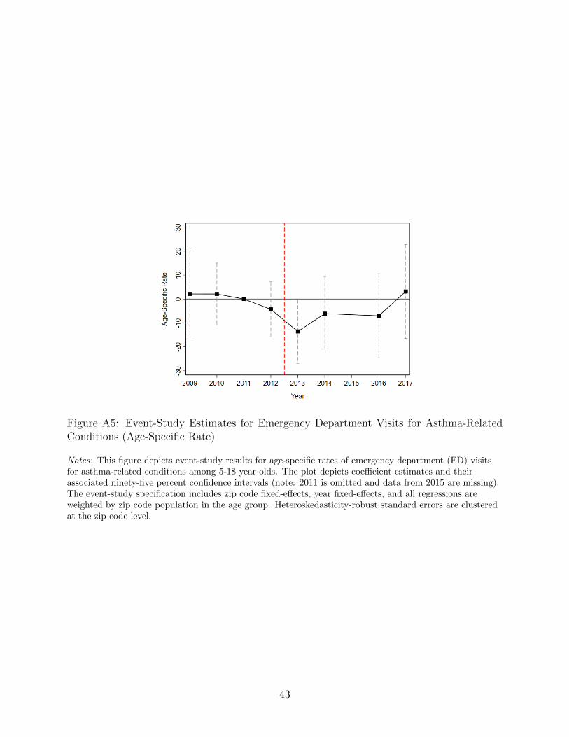
Figure A5: Event-Study Estimates for Emergency Department Visits for Asthma-RelatedConditions (Age-Specific Rate)
Notes: This figure depicts event-study results for age-specific rates of emergency department (ED) visitsfor asthma-related conditions among 5-18 year olds. The plot depicts coefficient estimates and theirassociated ninety-five percent confidence intervals (note: 2011 is omitted and data from 2015 are missing).The event-study specification includes zip code fixed-effects, year fixed-effects, and all regressions areweighted by zip code population in the age group. Heteroskedasticity-robust standard errors are clusteredat the zip-code level.
43
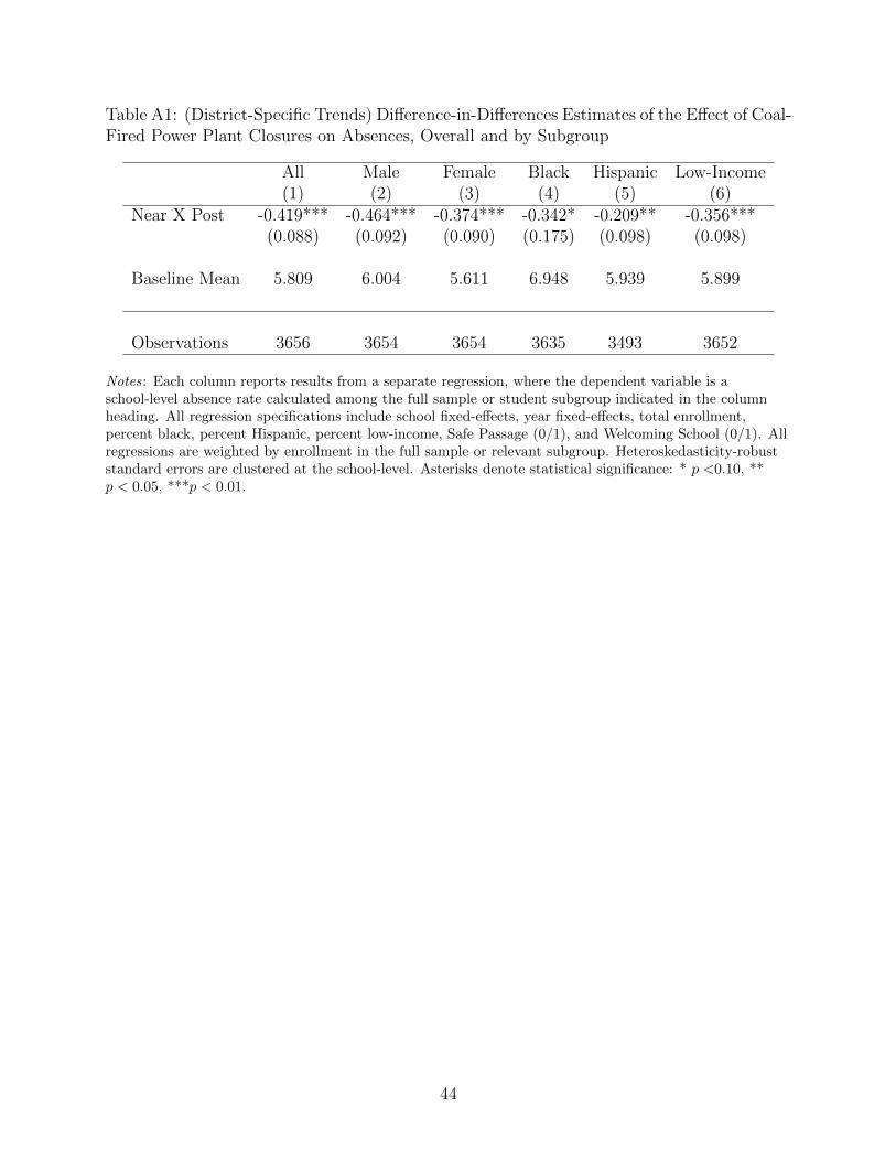
Table A1: (District-Specific Trends) Difference-in-Differences Estimates of the Effect of Coal-Fired Power Plant Closures on Absences, Overall and by Subgroup
All Male Female Black Hispanic Low-Income(1) (2) (3) (4) (5) (6)
Near X Post -0.419*** -0.464*** -0.374*** -0.342* -0.209** -0.356***(0.088) (0.092) (0.090) (0.175) (0.098) (0.098)
Baseline Mean 5.809 6.004 5.611 6.948 5.939 5.899
Observations 3656 3654 3654 3635 3493 3652
Notes: Each column reports results from a separate regression, where the dependent variable is aschool-level absence rate calculated among the full sample or student subgroup indicated in the columnheading. All regression specifications include school fixed-effects, year fixed-effects, total enrollment,percent black, percent Hispanic, percent low-income, Safe Passage (0/1), and Welcoming School (0/1). Allregressions are weighted by enrollment in the full sample or relevant subgroup. Heteroskedasticity-robuststandard errors are clustered at the school-level. Asterisks denote statistical significance: * p <0.10, **p < 0.05, ***p < 0.01.
44
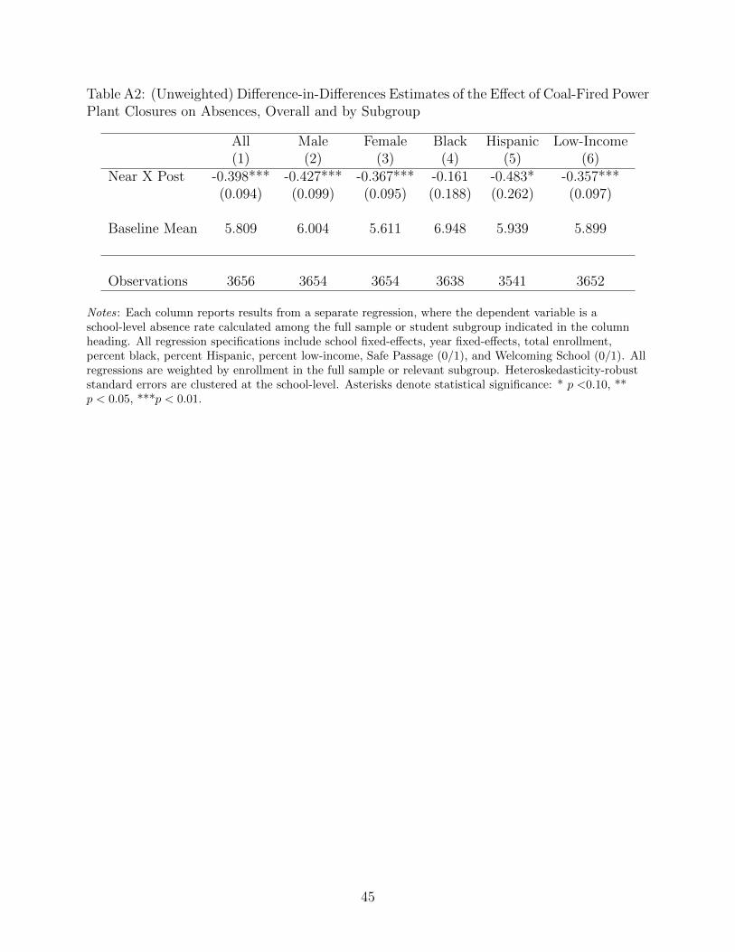
Table A2: (Unweighted) Difference-in-Differences Estimates of the Effect of Coal-Fired PowerPlant Closures on Absences, Overall and by Subgroup
All Male Female Black Hispanic Low-Income(1) (2) (3) (4) (5) (6)
Near X Post -0.398*** -0.427*** -0.367*** -0.161 -0.483* -0.357***(0.094) (0.099) (0.095) (0.188) (0.262) (0.097)
Baseline Mean 5.809 6.004 5.611 6.948 5.939 5.899
Observations 3656 3654 3654 3638 3541 3652
Notes: Each column reports results from a separate regression, where the dependent variable is aschool-level absence rate calculated among the full sample or student subgroup indicated in the columnheading. All regression specifications include school fixed-effects, year fixed-effects, total enrollment,percent black, percent Hispanic, percent low-income, Safe Passage (0/1), and Welcoming School (0/1). Allregressions are weighted by enrollment in the full sample or relevant subgroup. Heteroskedasticity-robuststandard errors are clustered at the school-level. Asterisks denote statistical significance: * p <0.10, **p < 0.05, ***p < 0.01.
45
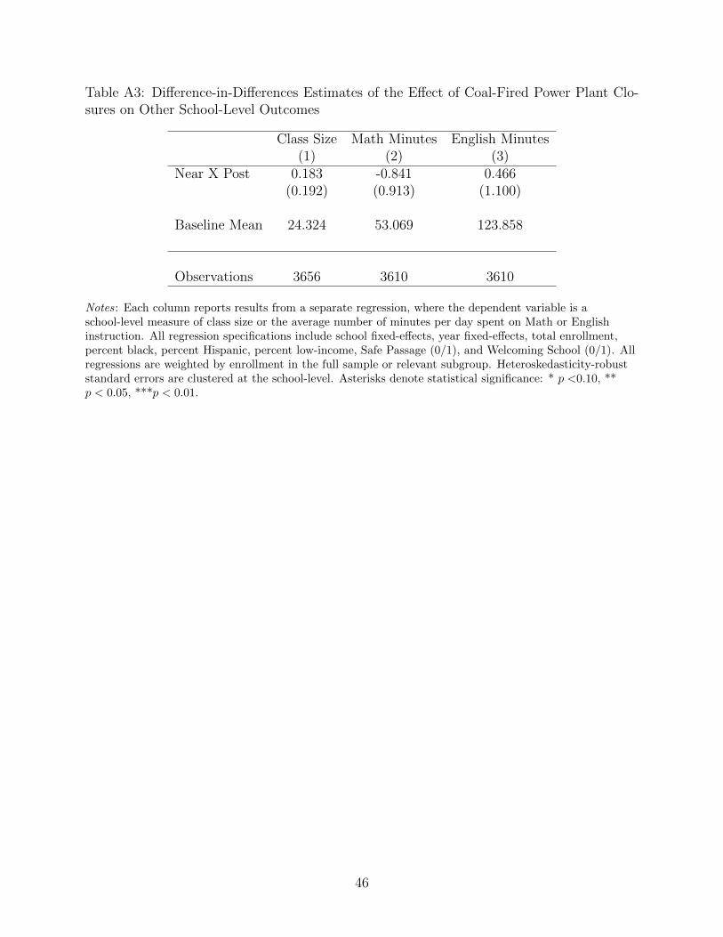
Table A3: Difference-in-Differences Estimates of the Effect of Coal-Fired Power Plant Clo-sures on Other School-Level Outcomes
Class Size Math Minutes English Minutes(1) (2) (3)
Near X Post 0.183 -0.841 0.466(0.192) (0.913) (1.100)
Baseline Mean 24.324 53.069 123.858
Observations 3656 3610 3610
Notes: Each column reports results from a separate regression, where the dependent variable is aschool-level measure of class size or the average number of minutes per day spent on Math or Englishinstruction. All regression specifications include school fixed-effects, year fixed-effects, total enrollment,percent black, percent Hispanic, percent low-income, Safe Passage (0/1), and Welcoming School (0/1). Allregressions are weighted by enrollment in the full sample or relevant subgroup. Heteroskedasticity-robuststandard errors are clustered at the school-level. Asterisks denote statistical significance: * p <0.10, **p < 0.05, ***p < 0.01.
46

Table A4: (SEs Clustered at Zip Code Level) Difference-in-Differences Estimates of theEffect of Coal-Fired Power Plant Closures on Absences, Overall and by Subgroup
All Male Female Black Hispanic Low-Income(1) (2) (3) (4) (5) (6)
Near X Post -0.395*** -0.440*** -0.349*** -0.431** -0.197* -0.337**(0.121) (0.118) (0.125) (0.216) (0.116) (0.140)
Baseline Mean 5.809 6.004 5.611 6.948 5.939 5.899
Observations 3656 3654 3654 3635 3493 3652
Notes: Each column reports results from a separate regression, where the dependent variable is aschool-level absence rate calculated among the full sample or student subgroup indicated in the columnheading. All regression specifications include school fixed-effects, year fixed-effects, total enrollment,percent black, percent Hispanic, percent low-income, Safe Passage (0/1), and Welcoming School (0/1). Allregressions are weighted by enrollment in the full sample or relevant subgroup. Heteroskedasticity-robuststandard errors are clustered at the school-level. Asterisks denote statistical significance: * p <0.10, **p < 0.05, ***p < 0.01.
47

Table A5: (Randomization-Based Inference) Difference-in-Differences Estimates of the Effectof Coal-Fired Power Plant Closures on Absences, Overall and by Subgroup
All Male Female Black Hispanic Low-Income(1) (2) (3) (4) (5) (6)
Near X Post -0.395*** -0.440*** -0.349*** -0.431** -0.197** -0.337***[0.000] [0.000] [0.000] [0.012] [0.021] [0.000]
Baseline Mean 5.809 6.004 5.611 6.948 5.939 5.899
Observations 3656 3654 3654 3635 3493 3652
Notes: Each column reports results from a separate regression, where the dependent variable is aschool-level absence rate calculated among the full sample or student subgroup indicated in the columnheading. All regression specifications include school fixed-effects, year fixed-effects, total enrollment,percent black, percent Hispanic, percent low-income, Safe Passage (0/1), and Welcoming School (0/1). Allregressions are weighted by enrollment in the full sample or relevant subgroup. Heteroskedasticity-robuststandard errors are clustered at the school-level. Asterisks denote statistical significance: * p <0.10, **p < 0.05, ***p < 0.01.
48

Table A6: Correlation Matrix, School Characteristics Related to Exposure and Percentageof Low-Income Students
Percent AC Wind Days Magnet (0/1) Percent Low-Income(1) (2) (3) (4)
Percent AC 1.0000Wind Days -0.0741 1.0000Magnet (0/1) -0.0737 0.0030 1.0000Percent Low-Income 0.0121 -0.1887 -0.0306 1.0000
Notes: Each cell reports a correlation coefficient calculated in the baseline school year (2008/09) among allschools in the sample. Correlation coefficients involving school-level air conditioning are only calculatedamong the subsample of schools from Chicago Public Schools (CPS).
49
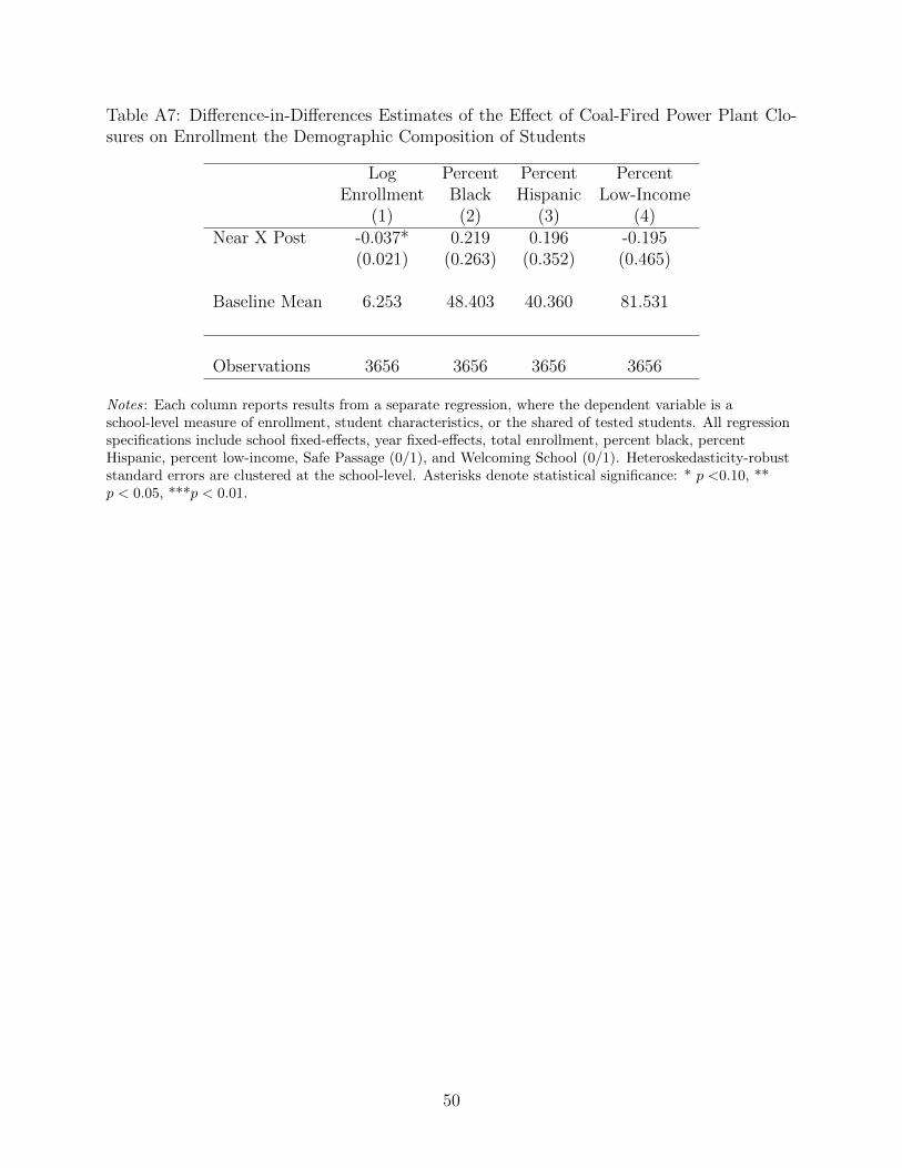
Table A7: Difference-in-Differences Estimates of the Effect of Coal-Fired Power Plant Clo-sures on Enrollment the Demographic Composition of Students
Log Percent Percent PercentEnrollment Black Hispanic Low-Income
(1) (2) (3) (4)Near X Post -0.037* 0.219 0.196 -0.195
(0.021) (0.263) (0.352) (0.465)
Baseline Mean 6.253 48.403 40.360 81.531
Observations 3656 3656 3656 3656
Notes: Each column reports results from a separate regression, where the dependent variable is aschool-level measure of enrollment, student characteristics, or the shared of tested students. All regressionspecifications include school fixed-effects, year fixed-effects, total enrollment, percent black, percentHispanic, percent low-income, Safe Passage (0/1), and Welcoming School (0/1). Heteroskedasticity-robuststandard errors are clustered at the school-level. Asterisks denote statistical significance: * p <0.10, **p < 0.05, ***p < 0.01.
50
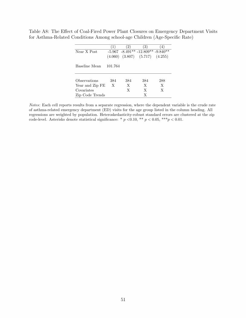
Table A8: The Effect of Coal-Fired Power Plant Closures on Emergency Department Visitsfor Asthma-Related Conditions Among school-age Children (Age-Specific Rate)
(1) (2) (3) (4)Near X Post -5.967 -8.491** -12.809** -9.840**
(4.060) (3.807) (5.717) (4.255)
Baseline Mean 101.764
Observations 384 384 384 288Year and Zip FE X X X XCovariates X X XZip Code Trends X
Notes: Each cell reports results from a separate regression, where the dependent variable is the crude rateof asthma-related emergency department (ED) visits for the age group listed in the column heading. Allregressions are weighted by population. Heteroskedasticity-robust standard errors are clustered at the zipcode-level. Asterisks denote statistical significance: * p <0.10, ** p < 0.05, ***p < 0.01.
51

Appendix B: Data Sources
K-8 Public School Enrollment Data
Public school locations and enrollments were obtained from the Elementary and SecondaryInformation System (ElSi) of the National Center for Education Statistics (NCES) of theUnited States Department of Education (2015/16 school year). These data are public-useand are available here: https://nces.ed.gov/ccd/elsi/.
Data on Operational Coal-Fired Power Plants
Coal-fired power plant locations, energy sources, and operational statuses were obtainedfrom the United States Energy Information Administration (EIA) Form EIA-860 for 2016.These data are public-use and are available here: https://www.eia.gov/electricity/
data/eia860/.
Illinois State Board of Education (ISBE) Report Card Data Library
Illinois State Board of Education Report Card Data are public-use and are available here:https://www.isbe.net/ilreportcarddata.
The annual aggregate absence rate is a ratio of the sum of all student absence days(summed across all students enrolled in the school) to the sum of all student enrollmentdays (summed across all students in the school). Let aist be the number of absence daysfor student i enrolled in school s in year t and let eist be the number of enrollment daysfor student i enrolled in school s in year t. Note that eist ≤ 180, since some students mayenroll (transfer in) after the first day or disenroll (transfer out) prior to the end of the school
year. The annual aggregate absence rate is then given by: Ast = ΣNg
i=1aist/eist, where gdenotes student group (either all students in the school, male students, female students, orlow-income students).
Air Quality Monitoring Station Data
We obtained daily data from Air Quality Monitoring Stations in Cook County, Illinois andLake County, Indiana for the years 2008-2016. These data are public-use and are availablehere: https://www.epa.gov/outdoor-air-quality-data/download-daily-data.
To produce time-series figures documenting annual average concentrations of sulfur diox-ide, fine particulates, and nitrogen dioxide, we used data from the following air qualitymonitoring stations located in Cook County, Illinois and Lake County, Indiana. We selectedthe stations below because they were the closest (distance listed below) to the Crawford,Fisk Street, and State Line Generating Stations:
• Sulfur Dioxide (SO2)
– Crawford: Cook County Trailer (3.86 kilometers)
– Fisk Street: Cook County Trailer (8.25 kilometers)
52
– State Line: Hammond CAAP (7.89 kilometers)
• Fine Particulates (PM2.5)
– Crawford: Liberty School (4.54 kilometers)
– Fisk Street: Liberty School (8.08 kilometers)
– State Line: Washington High School (2.66 kilometers)
• Nitrogen Dioxide (NO2)
– Crawford: Cook County Trailer (3.86 kilometers)
– Fisk Street: CTA Building (3.35 kilometers)
School Districts in Study
We included school-level data from the following fifteen school districts in Illinois in oursample:
1. Forest Park School District
2. Riverside School District
3. Oak Park Elementary School District
4. Berwyn North School District
5. Cicero School District
6. Berwyn South School District
7. Lyons School District, Summit School District
8. Central Stickney School District
9. Burbank School District
10. Oak Lawn-Hometown School District
11. Dolton School District
12. Burnham School District
13. Calumet City School District
14. City of Chicago Public Schools
53

Coal-Fired Power Plant Emissions Data
We obtained monthly emissions data from the EPA’s Air Markets Program Data.23 Thesemonthly generation data provide information about the current and historical patterns ofoperation of industrial sites. For this paper, monthly generation data were used for theperiod of 2008-2012 to calculate monthly capacity factors for the Crawford, Fisk Street, andState Line Generating Stations.
Wind Data
We obtained daily wind data from the Global Historical Climatology Network (GHCN)of the National Centers for Environmental Information (NCEI) of the National Oceanicand Atmospheric Administration (NOAA).24 These daily wind readings came from the landsurface station located at Midway Airport (MDW) in Chicago, Illinois (station number:USW00014819). We used daily readings on the direction (in degrees) of the fastest 2-minutewind (wdf2).
Air Conditioning Data in Chicago Public Schools (CPS)
We obtained information on air conditioning (AC) in CPS school buildings from a publishedreport of the Chicago Public Schools (CPS). This report was generated using the UnitedStates Environmental Protection Agency (US EPA) Energy Star Portfolio Manager. Thereport contained building level information on the percent of the school with air conditioningfrom April 2011.
Magnet School Status
We obtained information on schools’ magnet status from the Elementary/Secondary Infor-mation System (ElSi), a web application of the National Center for Education Statistics(NCES).25 These data came from the 2008/09 school year. Magnet schools typically donot have attendance boundaries, and spaces in magnet schools are allocated on the basis ofrandom lottery (following an application process).
Zillow Housing Value Data
We obtained zip code-level housing values from https://www.zillow.com/research/data/.According to Zillow, the Zillow Housing Value Index (ZHVI) is “[a] smoothed, seasonallyadjusted measure of the typical home value and market changes across a given region andhousing type. It reflects the typical value for homes in the 35th to 65th percentile range.”We used the smoothed, seasonally adjusted time series for all homes and converted levels ofnominal dollars to the natural logarithm of 2017 dollars.
23Air Markets Program data are available here https://ampd.epa.gov/ampd/.24These data are public-use and can be downloaded here: https://www.ncdc.noaa.gov/
ghcn-daily-description.25ElSi data are available here https://nces.ed.gov/ccd/elsi/.
54
Data on Emergency Department (ED) Visits for Asthma-RelatedConditions
We obtained annual counts of emergency department visits for children ages 0-4 and 0-18for asthma-related conditions at the zip code-level from the Chicago Health Atlas. Thesedata are public-use and are available here: https://www.chicagohealthatlas.org/. Theseannual counts were available for 48 zip codes (or zip code aggregates) for the years 2009-2017(excluding 2015, when no data were available). These data were derived from microdata fromthe Discharge Data, Division of Patient Safety and Quality, Illinois Department of PublicHealth. We subtracted these measures from one another to create our measure of the numberof visits among 5-18 year-old children, since this age group was closest to the population ofelementary school (K-8) students.
We calculated crude and age-specific emergency department (ED) visit rates (per 10,000inhabitants) for asthma-related conditions using zip-code level data from American Factfinder.26
Crude rates were calculated for by adjusting annual counts of ED visits for asthma-relatedconditions by total population, and age-specific rates were calculated using population countsfor age groups (5-18). We used population estimates for the age group 5-19 to calculate theage-specific rate for children ages 5-18 because more granular data were not available. Pop-ulation estimates (overall) and by age group came from the Decennial Census (2010) andthe American Community Survey (ACS) 5-Year Estimates (2011-2017). Data for 2009 werelinearly interpolated using the Decennial Censuses from 2000 and 2010.
Diagnoses included in the definition of asthma-related conditions can be found here:https://www.cdc.gov/asthma/data-analysis-guidance/ICD-9-CM-ICD-10-CM.htm. Wenote that the coding of this measure changed in 2015 (omitted from our data) due to transi-tion from the Ninth to the Tenth version of the International Classification of Disease (i.e.,ICD-9 to ICD-10).
26There data are public-use and are available here: https://factfinder.census.gov/faces/nav/jsf/
pages/index.xhtml.
55