Are America’s Inner Cities Competitive? Evidence from the 2000s

Daniel A. Hartley Senior Research Economist,

Federal Reserve Bank of Chicago

230 South LaSalle Street, Chicago, Illinois 60604-1413

(312) 322-5531 p daniel.a.hartley@chi.frb.org

Nikhil Kaza Associate Professor

Department of City and Regional Planning

University of North Carolina, Chapel Hill

110 New East Chapel Hill, NC 27599-3140

(919) 962 4767 p (919) 962 5206 f nkaza@unc.edu

T. William Lester (contact author)

Assistant Professor Department of City and

Regional Planning University of North Carolina,

Chapel Hill 320 New East

Chapel Hill, NC 27599-3140 (919) 962-3512 p (919) 962 5206 f twlester@unc.edu

ABSTRACT

In the years since Michael Porter’s research about the potential competitiveness of inner cities, there has been growing evidence of a residential resurgence in urban neighborhoods. Yet, there is less evidence on the competitiveness of inner cities for employment. The authors document the trends in net employment growth and find that inner cities gained over 1.8 million jobs between 2002 and 2011 at a rate comparable to suburban areas. The authors also find a significant number of inner cities are competitive over this period—increasing their share of metropolitan employment in 144 out of 281 metropolitan statistical areas. Also described by the authors is the pattern of job growth within the inner city, who find that tracts that grew faster tended to be closer to downtown, with access to transit and adjacent to areas with higher population growth. However, tracts with higher poverty rates experienced less job growth, indicating that barriers still exist in the inner city.

Key words:

JEL Codes:

Author Bios

Daniel Hartley is a policy economist in the Economic Research Department at the Federal Reserve Bank of Chicago. His primary fields of interest are urban and regional economics and labor economics. Dr. Hartley’s current work focuses on crime, public housing, foreclosures, and neighborhood employment dynamics.

Nikhil Kaza is an associate professor of city and regional planning at the University of North Carolina, Chapel Hill. He is interested in the institutional analysis of planning and the use of large data sets to measure the performance of cities.

2

T. William Lester is an assistant professor of city and regional planning at the University of North Carolina, Chapel Hill. His research focuses on the effectiveness of urban economic development policy and the impact of minimum wage and living wage policies on urban economic development.

3

In the years since Michael Porter’s seminal research about the potential competitiveness of

inner cities, two narratives have emerged about the overall pattern of urban economic

development. The first, which we call the “comeback cities” narrative, states that the decades of

the 1990s and 2000s were a renaissance for cities, as flows of population, jobs, and investment

shifted back from suburbs and exurbs to urban areas, particularly to downtowns. The literature

on gentrification, as well as the oft-cited creative class theories of Richard Florida, underscore

this narrative by highlighting the pro-urban preferences and consumption patterns of a new,

rising middle class (Florida, 2003; Smith, 2002; Zukin, 1982). The second narrative that has

taken shape is that of an uneven geography of growth in the last few decades. The literature on

high technology regions argues that contemporary U.S. economic development has taken on a

distinctly uneven pattern that leads to a polarization between so-called “innovative” regions and

“backward” regions, which in turn drives inequality and a divergence in outcomes across

metropolitan areas (Moretti, 2012; Pastor, Lester, & Scoggins, 2009; Saxenian, 1994).i The

implication of this second narrative is that the type of inner-city renaissance described in the first

narrative will only occur in growing, innovative regional economies. However, is this

necessarily the case? Can inner-city economic growth occur in declining regions? Recent

research has demonstrated an empirical link between gentrification and neighborhood job growth

(Lester & Hartley, 2014). Yet, is the type of consumption-based growth that is fueled by

gentrification in growing regions like New York or the San Francisco Bay Area the only

mechanism to bring jobs back to urban neighborhoods? Or can robust job growth stem from

expansion of anchor institutions in nontradable sectors such as universities and health care

institutions (Adams, 2003; Harkavy & Zuckerman, 1999)? In addition to private market-driven

development, policy makers have employed a host of economic development tools and

4

distributed millions of dollars in funding targeted toward business development and job growth

in inner-city neighborhoods. Have tools such as targeted tax credits (e.g. Empowerment

Zone/Enterprise Community designation, Low Income Housing Tax Credit [LIHTC]) influenced

the pattern of inner-city employment growth? In this study, we explore these intertwined

narratives by describing the pattern of neighborhood-based employment changes at a national

scale. We then test the validity of a number of competing claims about the competitiveness of

inner-city neighborhoods in terms of economic development during the 2000s.

First, using data at the census tract level from the Local Origin-Destination Employment

Statistics (LODES) program at the U.S. Census Bureau, we begin by providing an overview of

the extent and broad characteristics of employment growth of inner cities, central business

districts (CBD), and suburban areas of all metropolitan areas in the United States. Surprisingly,

we find that the rate of job growth between 2002 and 2011 in inner cities—defined broadly as

non-CBD tracts in the largest principal city within a metropolitan area—was on par with that of

suburban areas (6.1% versus 6.9%) and even surpassed suburbs in the post-Great Recession

recovery (2009-11). This trend is consistent across broad census regions. Yet, this trend is less

pronounced—though still positive—when we focus only on portions of the inner city that were

more economically distressed at the start of the 2000s.

Next, we explicitly test the question of inner-city competitiveness by identifying

metropolitan areas that had both net positive employment growth and an increase in the share of

jobs located in the inner city (these two criteria form our working definition of competitive inner

cities). We find 144 metropolitan statistical areas (MSA) with competitive inner cities using our

broad definition of inner city tracts and 85 using the narrower method. These MSAs are diverse

5

geographically, but compared to other metropolitan areas, tend to have above-average growth in

high-wage jobs, less racial segregation, and less job sprawl.

Finally, we provide a third descriptive analysis of the spatial determinants of inner-city

growth at the tract level within inner-city areas. Specifically, we find that inner-city employment

growth is positively associated with neighborhoods closer to downtown, with nearby population

increases, recent residential construction, and other indicators of gentrification. We also find that

employment grew faster in areas with mixed uses and greater employment diversity. There is

some evidence that empowerment zone designation is associated with more employment growth;

however, tracts with high poverty levels have lower job growth. Within economically distressed

inner-city areas, these findings are very similar, although job growth is driven less by indicators

of gentrification and is more closely associated with the expansion of anchor institutions.

The remainder of the study is organized as follows: The second section reviews the research

on the competitiveness of inner cities and puts our empirical analysis in the context of the

literature inspired by Porter’s work. The third section describes the main data sets and analytical

methods used in our analysis. This is followed by a section on the descriptive analysis of the

patterns of inner-city job growth in aggregate and describes our analysis of the characteristics of

regions with competitive inner cities. The fifth section presents our model of tract-level

correlates of inner-city employment growth. The final section concludes the study and

summarizes our descriptive analysis of the nature of inner-city job growth in the 2000s.

Literature Review

6

Writing in 1997 in this journal, Michael Porter made a strong and influential argument

that inner-city areas had important and “unrecognized” competitive advantages as a business

location. Specifically, he called for a private-sector-led economic development strategy that

leveraged the strategic location of inner-city neighborhoods (near the CBD and key

infrastructure), and the integration with existing regional economic strengths as well as the local

purchasing power and human resources of inner-city residents (Porter, 1997). While he

recognized a significant role for government (and nonprofits), Porter also helped to highlight

regulatory barriers of high taxes and red tape that prevented further private-sector investment.

Looking back at his strategic recommendations and comparing them to current practice, it is easy

to see how influential they have been, as few contemporary urban economic developers or

planners would find much to disagree with.ii However, it is important to recall the context in

which he was writing. Although the mid-1990s was a period of significant economic growth for

the United States, it followed nearly two decades of economic restructuring that significantly

altered the economic role of central cities and changed the geography of employment

opportunities throughout most metropolitan areas in the country.

The decades of the 1970s and 1980s were characterized by a pattern of economic

restructuring that featured the dual trends of massive manufacturing job losses coupled with the

continued suburbanization of population and employment. These trends significantly reduced

the base of job opportunities for residents of inner-city neighborhoods, which once housed many

of the goods-producing jobs and a predominantly working-class workforce. The problem of

declining employment in older, inner-city neighborhoods and growth in emerging suburban areas

was first recognized in the late 1960s by scholars like Kain (1968), who argued that housing

discrimination coupled with lack of opportunity in urban areas led to persistently high

7

unemployment of minority workers in inner cities. Although the “spatial mismatch” hypothesis

has been a widely debated topic in the social sciences (see Chapple, 2006; Ihlanfeldt & Sjoquist,

1989; Teitz & Chapple, 1998), the declining employment within inner-city neighborhoods was

widely viewed as a critical problem. To get a sense of how profoundly scholars viewed the

problem of the inner city in the mid-1990s, we recall here the opening lines of Galster and

Killen’s (1995) article on the geography of metropolitan opportunity, as follows:

Horatio Alger lies dead in the streets of the inner city. For millions of Americans, the rags-to-riches fable has been reduced to ashes just as surely as have many blocks in South Central Los Angeles and other desperate inner-city communities. What once was a spring board of socioeconomic mobility for generations…has for too many been transformed into a pit in which perpetual deprivation and social dysfunction reign. (Galster & Killen, 1995, 7)

Scholars from a wide variety of disciplines attempted to diagnose the problems associated

with lack of inner-city employment opportunities, linking it broader issues of neighborhood

decline including high crime, persistent poverty, segregation, and changing attitudes toward

work (Kasarda, 1993; Katz, 1993; Wilson, 1987, 1996).

The issue of declining inner-city employment and population losses, coupled with

continued suburbanization and sprawl, also spawned concerns that declining central cities could

pose a drag to an entire region’s economic growth. This, in turn, ignited a series of studies

specifically focused on the question of whether or not suburbs could prosper without their central

cities (Hill, Wolman, & Ford, 1995; Ledebur & Barnes, 1993; Voith, 1992 1998). Pack’s (2002)

comprehensive analysis of long-term trends in metropolitan economic performance bears this

out. Between 1960 and 1990, the share of income earned by central-city residents declined from

45% to 30% and rose in suburban areas from 55% to 70% (Pack, 2002, p.3). Although a great

8

deal of empirical work focused on the issue of inner-city competitiveness and the

interdependency of suburbs and cities, eventually a consensus emerged supporting the idea that

the economic health of both areas was closely linked by regional factors. Voith (1992)

concluded that “decline in central cities is likely to be associated with slow-growing suburbs.

Even if the most acute problems associated with urban decline do not arise in the suburbs, central

city decline is likely to be a long-run, slow drain on the economic and social vitality of the

region.” (Voith, 1992, p.31)

Just as the attention of federal policy makers shifted away from defining economic

challenges in stark urban versus suburban terms, the academic literature shifted in the following

decade to questions of the determinants of overall metropolitan economic competitiveness. The

key question here was what factors explained the relative economic health and resilience of some

metropolitan regions, particularly those with a growing high-technology industrial base. The

work of Saxenian (1994), Storper (1997), and others argued that metropolitan areas that featured

regionally based networks of firms and supporting institutions that foster accelerated innovation

were ultimately more resilient to economic restructuring and as a result, are more competitive in

terms of employment and income growth. This emphasis on innovation and regional

competitiveness in the economic development literature had a profound impact on practice

(Clark, 2013) and shifted the focus away from intrametropolitan disparities, and instead

highlighted the overall uneven pattern of metropolitan growth in the 1990s and 2000s.

Starting in the early 2000s, a new narrative began to emerge on “comeback cites” as

many scholars used newly available census data to identify a growing trend of residential growth

particularly focused in the downtown and nearby areas of older central cities (Sohmer & Lang,

2001). Much of this research highlighted shifting demographics, such as the aging of the

9

population (i.e., empty nesters without children) and changing preferences for high-amenity

locations like downtown as the causes of residential resurgence of downtown areas. This

research is largely congruent with a preexisting literature on the causes and consequences of

gentrification. What began as a niche field that focused on select neighborhoods in places like

the Lower East Side in New York (Smith, 1996) or the South End in Boston and was initially

considered a relatively small trend (Wyly & Hammel, 1999), has now grown to be an active

literature drawing scholarship from a wide variety of disciplines. Whereas much of the

empirical debate in the gentrification literature focused on measuring the extent of displacement

(Freeman, 2005; Marcuse, 1985; Vigdor, 2002) within individual cities, there is growing

consensus that gentrification is part of a broader demographic shift that results in the influx of

better-educated and high-income households to formerly low- and moderate-income inner-city

neighborhoods. The drivers of this trend are seen to involve changes in the consumption and

locational preferences of what some sociologists called a “new middle class” (Ley, 1996) and

what Richard Florida (2002) later termed the “creative class.” Regardless of their moniker,

members of this demographic subgroup favor urban living and the greater accessibility it affords

over the suburban dream of previous generations. According to these scholars, such preference

shifts also drive gentrification by increasing demand for urban entertainment and consumption

spaces for the new high-income residents (Lloyd & Clark, 2001; Zukin, 1982).

While scholars continue to debate how widespread and significant gentrification is as a

demographic trend and what it will ultimately mean for inner cities, there is a growing literature

that has examined the impact of gentrification on employment within inner-city neighborhoods.

Curran (2004, 2007) focused on a single neighborhood – Williamsburg in Brooklyn—and found

that new residential growth led to displacement of nearby industrial jobs. Meltzer and Schuetz

10

(2012) showed that neighborhood retail grew faster in New York City neighborhoods that

experienced gentrification. More recently, Lester and Hartley (2014) examined the impact of

gentrification at the census-tract level using detailed employment data for 29 large cities in the

United States, and found that gentrifying neighborhoods had faster employment growth and a

more rapid shift between traditional blue collar work and locally oriented services such as

restaurants and entertainment. Beyond these studies, there have been relatively few studies that

specifically look at the nature of employment growth in inner cities. There have been individual

case studies such as Hutton’s (2004) description of the emergence of new high-tech industry

clusters in Vancouver, British Columbia. In addition, there are two new reports that focus on the

long-term residential shifts of poor neighborhoods in U.S. metropolitan areas, which suggest that

the gentrification or “back to the city” trend may be limited or is bypassing high-poverty

neighborhoods. Specifically, Cortright and Mahmoudi (2014) find that 69% of census tracts

with high poverty levels (30%) in 1970 still had high poverty levels in 2010. Aliprantis, Fee, and

Oliver (2014) examine patterns of tract-level income change between 1980 and 2010 and find

considerable stability in tract-level income quartiles over time. However, they also find that

tract-level income growth varied widely by metropolitan characteristics, as tracts that

transitioned from poor to nonpoor were more likely to be located in growing metropolitan areas

that were relatively large and densely populated and that experienced greater immigration.

In addition to the gentrification literature, there is also a growing literature on the role of

immigrants in reversing the declining population of inner cities and supporting the economic

revitalization of urban neighborhoods. For example, Chicago’s small population increase

between 1990 and 2000—a reversal of three decades of decline—was driven by large increases

in foreign-born populations. Some scholars highlight the positive impact of immigration for

11

inner-city neighborhoods. For example, Sampson (2008) shows that neighborhoods with a

higher share of foreign-born residents have lower rates of violent crime. Also, Porter and Zhuo

(1992) find that high levels of social capital in tight immigrant-ethnic enclaves can lead to

greater entrepreneurship among some immigrant groups. As Bates (1997a, 2011) points out,

however, significant barriers remain, such as access to capital, that limit immigrant and minority

entrepreneurship .

Given the potentially conflicting evidence about demographic trends affecting the inner

city and the relative paucity of research on recent inner-city employment trends, we argue that

there is a need for a comprehensive analysis of job growth in America’s inner cities over the past

decade. Porter (1997) recognized this need early on, but lamented that there was no single

source of localized workplace-based employment statistics to track the changing economic role

of inner-city neighborhoods and to assess how much private investment “already recognized” the

competitive potential of the inner city.

Now we have such a data source, namely the Local Origin-Destination Employment Statistics

(LODES) (see below). Ultimately, this study will use a descriptive approach that revisits some

of the key questions in the preceding literature. First, we assess the actual extent of job growth

that has occurred in America’s inner cities relative to suburban areas and CBDs between 2002

and 2011, highlighting key differences by broad geographic regions, industrial sector, and tract

poverty status. Next, we return to the question of inner-city competitiveness by defining a new

methodology for identifying which regions have competitive inner cities and what distinguishes

them from the rest of the metropolitan areas. Finally, we test some of the predictions of the

gentrification literature and build a simple descriptive model of inner-city job growth at the tract

level.

12

Data Sources and Methodology

We primarily use data from the U.S. Census Bureau’s Longitudinal Employment and

Household Dynamics (LEHD) data set. Specifically, we use special tabulations of the LEHD

data created for local transportation and workforce development analysis called the Local Origin-

Destination Employment Statistics (LODES) program. The data set is available at a 2010 block-

group-level geography. Total employment and employment by broad industry sector from 2002

through 2011 are summarized to a tract level for the purposes of this analysis. Although the data

set is available for the most of the United States, some states are missing from the analysis

because of data nonavailability for the full period of analysis. These include Arizona, Arkansas,

the District of Columbia, Mississippi , New Hampshire, and Massachusetts, which began

participation in the LEHD at various years throughout the period and therefore do not figure in

the current analysis.

Although the LODES data are also available on a worker residence basis, we use

workplace-based counts of employment, as we are primarily interested in the changing

geography of employment between inner-city tracts and other components of metropolitan areas.

The LODES data set is a synthetic dataset derived from confidential data sources such as

unemployment insurance records, Topologically Integrated Geographic Encoding and

Referencing (TIGER) line files, and additional administrative data from the U.S. Census Bureau

and the Social Security Administration. Noise is then infused into the workplace totals to protect

employer and employee confidentiality. These data production methods and caveats should be

considered while evaluating the evidence presented in this analysis. For a more complete

description of the LODES data set and its differences with the standard census products such as

the American Community Survey (ACS), refer to Graham et.al (2014).

13

Although the LODES is a relatively new data source for examining employment

dynamics at small geographic scales, there is no reason to believe that it is inaccurate or that the

statistical “fuzzing” used to protect confidentiality would produce biased estimates. First, as

Abowd et. al. (2009) describe, the noise introduced to the data does not vary by geographic

location in a way that is systematically correlated with our definition of inner city versus suburb

status.iii Second, the LODES is now widely used in transportation planning and in the

transportation literature (see Owen & Levinson, 2015; Schleith & Horner, 2014).

Identifying the Inner City

As discussed above, although there is significant research on the competitiveness of inner

cities, it is very difficult to find a commonly accepted definition in the literature as to what

constitutes an inner-city area. Generally speaking, inner cities are understood as relatively poor

areas with high concentrations of minorities within large central cities. While nearly all scholars

distinguish the inner city from suburban areas and traditional downtowns, there is little

agreement on the essential characteristics of inner-city neighborhoods. Porter implies that these

areas are “distressed neighborhoods, in which, in most cases, African Americans and other

people of color represent the majority of the population” (Porter, 1997. p. 11). Yet, more recent

studies, such as Hutton (2004), simply look at all nondowntown portions of the central city.

Ultimately, the literature lacks a systematic delineation of the geographic or jurisdictional extent

of inner cities. As a first approximation, we define inner cities as areas of the largest central city

or cities in a metropolitan statistical area that are not part of the central business district. To

identify the main central cities in each MSA, we consider the official set of Principal Citiesiv

within an MSA (as defined by the U.S. Census Bureau) and select those principal cities that

collectively make up more than half of the principal city population within the MSA. Such

14

identification of main cities in an MSA eliminates classifying older suburban satellite cities (e.g.,

Schamburg, IL) as inner cities, but retains the flexibility of having multiple inner-city clusters

within an MSA. For example, in Minnesota, both Minneapolis and St. Paul are considered the

main cities and the tracts that are not within the CBDs of these cities are considered inner-city

areas. In general, a vast majority of the 281 MSAs considered in this analysis have only one

main central city from which we draw our definition of inner-city tracts.

Given the lack of consensus on how to define the inner city for data collection purposes,

we use two general methods. First, we take all census tracts within the largest(s) principal city

that are outside of the CBD. We call this the “broad” definition of inner city. Next, we follow

Porter’s original definition and further narrow this set of tracts to those that meet the following

criteria: a) The tract has a median household income that is below 80% of the MSA median

income in 2000, and b) The tract also has an unemployment rate greater than 25% above the

unemployment rate in 2000 (see Porter (1997), footnote 1). We refer to this narrower definition

as the “Porter definition.”

Identifying the Central Business District

To classify census tracts as inner city or not inner city, we needed to clearly define the

central business district or clearly define the downtown of each principal city. In addition to lack

of definition of inner city, there is also no accepted current definition and delineation of a CBD.

The last known delineation of the CBD was done in 1982 by the U.S. Census of Retail Trade. To

update this identification, we first identify all employment centers in an MSA. We then identify

the cluster of employment centers that overlap the point definitions of a CBD, provided by Fee

and Hartley (2011) and call them the central business districts within the MSA.

15

The employment centers are identified using methods detailed by McMillen (2001,

2003). Briefly, we construct a locally weighted regression using employment densities at a tract

level. The weighting function is a smoothing function that accounts for the spatially nearest 50%

of the density values. A tract is identified as an employment center if the residuals are

significantly greater than zero, accounting for the standard error of the estimate. This

nonparametric method has been used to identify employment centers in a number of studies

(Garcia-López, 2010; Suárez & Delgado, 2009). Once the tracts that have a higher than expected

residuals are identified within an MSA, a contiguity matrix is constructed using “spdep”

(Bivand, 2015). The contiguity matrices converted to a graph where nodes are the identified

census tracts and a pair of nodes have an edge if the corresponding contiguity matrix element is

nonzero using “igraph” (Csardi & Nepusz, 2006). Once the graph is constructed, standard graph

theoretic methods are used to decompose the graph into maximally connected components. If

any of the census tracts within a maximally connected cluster overlaps with the CBD point, then

we designate the entire cluster as a central business district.

[FIGURE 1 ABOUT HERE]

To conduct our descriptive analysis comparing metropolitan regions with competitive

inner cities to other regions, and for our tract-level determinants of inner-city job growth, we also

draw upon several other data sources. The two main sources of additional data beyond the

LODES data set are the Smart Location Database (SLD) produced by the U.S. Environmental

Protection Agency (EPA)v and the Building Resilient Regions (BRR) database (Pastor,

Scoggins, Lester, & Chapple, 2009). The BRR database is a comprehensive data set on

demographic, economic, and policy variables for all metropolitan areas in the United States

16

(mainly derived from census data) and was produced by the MacArthur Foundation’s Building

Resilient Regions research network (see Pastor et. al, 2009, for more information).

Employment Trends and the Competitiveness of Inner Cities

The Nature of Inner-City Employment Change in the United States in the 2000s

Compared to the preceding two decades, the 2000s was a period of relatively stable job

growth for America’s inner cities. During the 9-year period from 2002—just after a mild

recession—to 2011, 2 years after the end of the Great Recession—inner-city census tracts added

1.8 million net new jobs. Surprisingly, this rate of growth (6.1%) was roughly comparable to the

rate of growth observed in suburban areas (6.9%). However, suburbs still added nearly twice as

many total positions and maintained the preponderance of all metropolitan jobs Over the study

period, inner-city areas grew faster than nonmetropolitan areas (2.3%) and CBDs, which

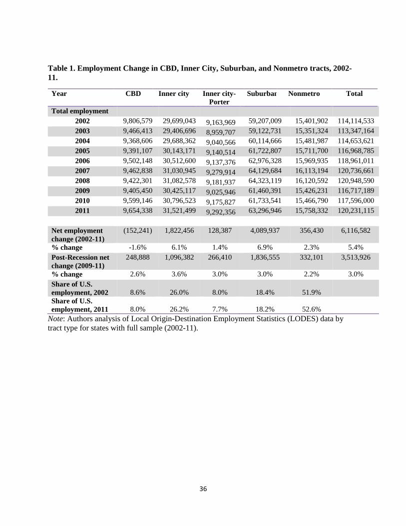
declined by 1.6%. As indicated in Table 1 below, the post-Great Recession period (2009-2011)

was particularly favorable to inner cities, as its growth rate actually surpassed the suburban rate

(3.6 versus 3.0) and nearly 1 in 3 jobs created during this period was located in the inner city.

While the more economically distressed parts of inner cities, as identified by the Porter

definition, experienced slower employment growth over the full period from 2002-2011, they

almost kept pace with the rest of the inner city and did keep pace with the suburbs during the

post-recession period, showing employment growth of 3%.

[TABLE 1 ABOUT HERE]

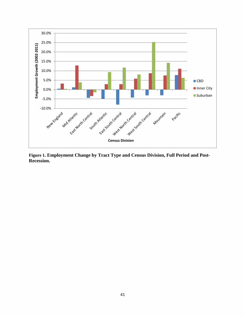
Given some concern in the literature that the “comeback cities” narrative is limited

primarily to only a select set of coastal cities such as New York, Washington, and San Francisco,

we examined the same employment trends in each of the nine census divisions across the country

17

(see Figures 2a and 2b). Looking at the full period, this observation still somewhat holds.

Although inner city growth was positive in all divisions except the East North Central (which

declined as a whole), it outpaced suburban areas in only the Mid Atlantic (which includes New

York) and the Pacific census divisions.

[FIGURE 2 ABOUT HERE]

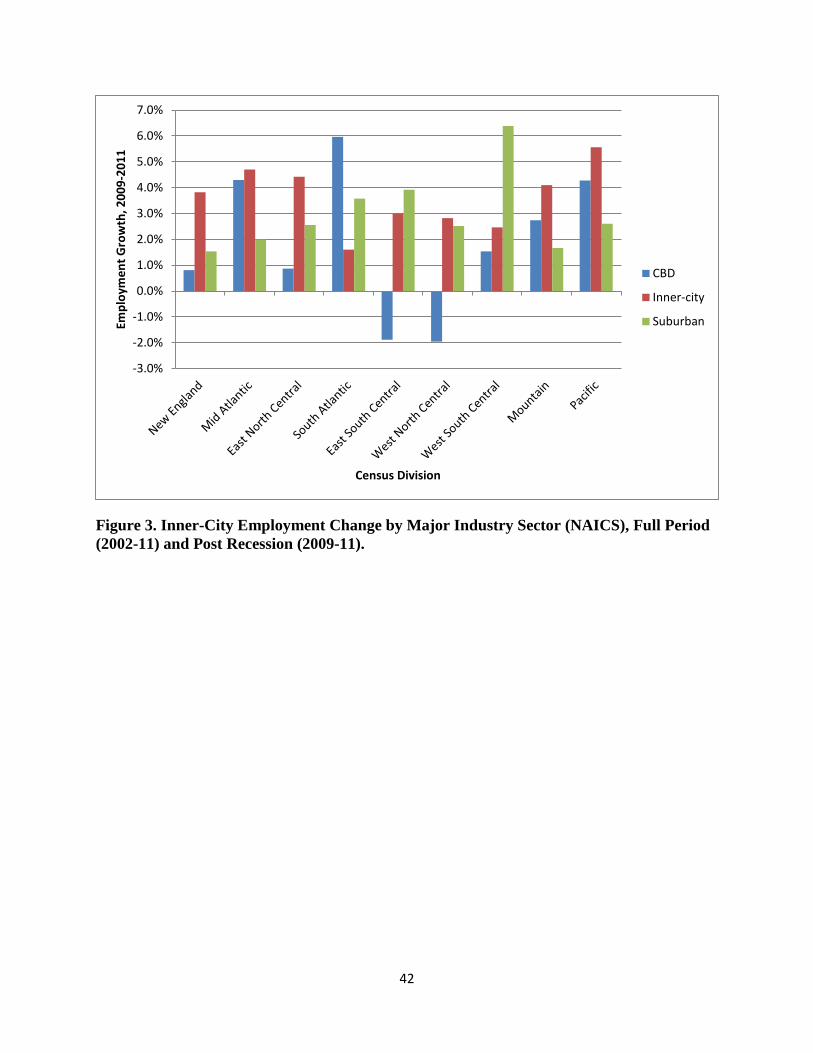
In the post-recession period, however, inner cities were considerably more competitive vis-à-vis

the suburbs throughout the country, growing faster in five out of nine divisions and rebounding

strongly even in the Rustbelt East North Central area. In this chart (Figure 2b), the outlier region

seems to be West South Central, where suburban job growth consistently swamped both CBD

and inner-city areas. Although this is a relatively small period, the post-recession evidence is

indicative of a relatively urban-based recovery.

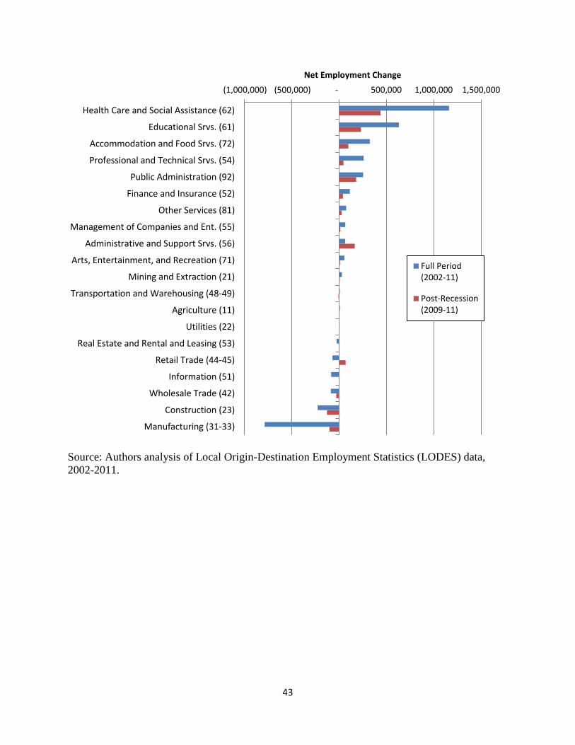
Whereas total employment increased within inner-city tracts in aggregate, there have

been significant industrial shifts occurring within inner cities as they continue to transition away

from goods-producing sectors and toward relatively place-bound service-sector industries. In

Figure 3, we analyze net employment change for the full period (2002-11) and the post-recession

period for all of the tracts defined as inner city for the United States as a whole. Not

surprisingly, the greatest losses occurred in manufacturing (-782,000 jobs), followed by

construction (-224,000), which was particularly hard hit by the housing crisis and recession.

The strongest-gaining industries were the so-called “eds and meds” sectors of Health Care and

Social Assistance and Educational Services, which added 1.1 million and 633,000 jobs,

respectively. This finding makes sense because many institutions such as universities and

hospitals were founded in the past century in inner-city neighborhoods, have remained in those

18

neighborhoods, and have proved resilient to the wider economic changes that affected the inner

city during the 1970s and 1980s. The economic role of universities and their expanding hospitals

is critical in areas like West Philadelphia (home to the University of Pennsylvania and Drexel

University) and Hyde Park (home to the University of Chicago). Inner-city areas also saw strong

growth in the Accommodation and Food Services (323,000) sector, which includes restaurants,

and is consistent with the findings in the gentrification literatures on the changing economic role

of inner cities from spaces of production to spaces of consumption.

[FIGURE 3 ABOUT HERE]

Because our definition of inner city is quite broad, including all non-CBD portions of the

largest principal city in each MSA, we also sought to understand if the net positive employment

growth was limited to areas that were initially higher-income enclaves within the city. To test

this, we categorized each census tract by its poverty status in 2000. Since much of the literature

in the 1990s focused on high poverty neighborhoods and declining employment therein, we also

included the tract poverty status in 1990.

[TABLE 2 ABOUT HERE]

As Table 2 indicates, the large majority of inner-city job creation occurred in areas where

less than 20% of residents earned incomes below the poverty line (79% for 1990 and 73% for

2000). In addition, lower poverty areas maintained a much larger share of total jobs (by a

factor of 2) compared to high poverty tracts. What is interesting about this tabulation is that the

figures for high-poverty tracts are positive at all, given all the preceding discussion of job flight

and neighborhood decline. Most interestingly is the fact that, although they only have a small

19

share of total jobs, the growth rate of tracts with extreme poverty (over 40%) was faster than

low-poverty tracts.

Inner-City Competitiveness at the Metropolitan Scale

The decade of the 2000s was significant in the long-term economic trajectory of inner

cities over the past 40 years because it marked a reversal of the trend of large-scale job losses

and decline. However, does this necessarily mean that inner cities are now more competitive

locations for business expansion and job growth compared to suburban areas? We revisit the

question of inner-city competitiveness by exploring the nature of inner-city job growth in nearly

all metropolitan areas in the United States, and attempting to determine the extent of inner-city

competitiveness and the regional factors that influence the growing competitiveness of inner

cities in certain MSAs.

However, the uneven pattern of metropolitan growth itself clearly plays a role for the

prospects of inner city change. In general, larger MSAs experienced larger total employment

growth over the study period. Places like San Antonio, TX and Los Angeles, CA experienced

substantive growth in metropolitan employment change and experienced significant growth in

inner-city employment. However, metropolitan area growth does not always coincide with

employment growth in the inner city. For example, in places like Houston and Dallas, TX, while

the inner-city employment growth is positive, suburban growth overshadows the inner city.

Therefore, we wanted to develop a method of defining inner-city competitiveness that accounted

for overall metropolitan growth and identified MSAs where job growth was disproportionately

focused on the inner city during the 2000s.

[FIGURE 4 ABOUT HERE]

20

To identify which inner cities are competitive over our study period, we examined the

relative change in the proportion of inner-city employment within its metropolitan area (see

Figure 4). Within each quadrant, we plot the 2002 inner-city share and 2011 inner-city share of

total metropolitan area employment. We then divide the entire data set into four groups based on

whether or not total employment in the metropolitan area grew or declined (horizontal axis) and

whether or not there was net positive inner-city job growth (vertical axis). Whereas there are a

few inner cities that have grown despite the overall metropolitan area decline (southeast

quadrant), the vast majority of observations with positive inner-city-employment growth also had

positive regional growth. However, because we are interested in “competitive” inner cities, we

focus on those metropolitan areas where inner cities increased their share of jobs. These metros

are above the 45° line in the bottom right corner of Figure 4. Specifically, we find that 120 out

of a total set of 281 metropolitan areas (43%) have “competitive inner cities.” We label these

metros as competitive inner cities and compare their characteristics with the other metropolitan

areas in the sample. Appendix A provides a complete list of these metropolitan areas. The

metropolitan areas that are on this list are quite diverse, ranging from large metros to more

moderate size ones. In general, the change in the share of employment in the inner city is modest

between 2002 and 2011, except in a few metropolitan areas.

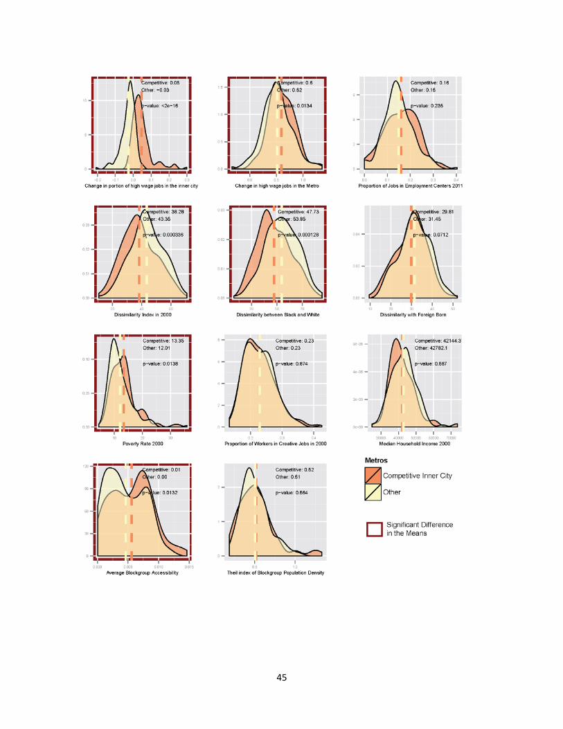
Next, we compared these metropolitan areas with competitive inner cities to the rest of

the metros in the sample (see Figure 5). There is no difference between proportions of jobs in

the concentrated employment subcenters between the two groups (as defined using McMillen

2003’s method); however, high-wage job growth, both at the metro level and within the inner

city, stand out. Competitive inner cities, in general, have experienced significant high-wage job

21

growth. Further research is needed to address the question of whether this high-wage job growth

is a cause or an effect of “competitiveness.”

[FIGURE 5 ABOUT HERE]

Metropolitan areas that have a lower Black-White dissimilarity index—an indicator of

segregation at the metro level—are more likely to have a competitive inner city. This is

consistent with the work of Pastor (Pastor, Drier, & al., 2000) and others who argue that regions

where segregation is less pronounced are more likely to produced balanced economic growth.

We find that metros with competitive inner cities have lower average Black-White dissimilarity

indices in 2000s compared to their peers. However, the two groups have the similar distribution

of dissimilarity indices with the foreign born and native born, suggesting a smaller influence of

cross-national migration on competitive inner cities.

Competitive inner-city metropolitan areas had higher poverty rates in 2000, suggesting

higher poverty rates are not a constraint for economic development. There are only small

differences in the means of the median household income between the two groups; however, the

means tell only part of the story. The distributions are quite different. The median income

distribution of the competitive metropolitan areas is skewed to the left compared to the rest of the

metros. Furthermore, higher poverty rates, especially in inner cities, might suggest

redevelopment opportunities. Metropolitan areas with competitive inner cities, on average, have

higher average job accessibility. Accessibility is measured at the block group level as the

percentage of the jobs in the metro that can be accessed within a 45-minute commute. This

difference disappears when we compare the average block group accessibility based on transit

service. Although we should expect to see higher competitiveness of metros with high quality

22

transit, this result is likely because of persistent low levels of transit provision and usage in the

United States.

Neither the population distribution nor the proportion of creative jobs is significantly

different from the rest of the metros in the competitive metropolitan areas. The Theil index of

population density represents skewness in the population density distribution. Higher Theil index

metropolitan areas are metros with some tracts with large population densities and the rest very

low population density, while a lower Theil index means the metropolitan area has relatively

uniform population density. The results suggest that concentrations of density are not different

between the two groups of the metropolitan areas.

We repeated the metropolitan-level competitiveness analysis using the narrower Porter

definition of inner-city tracts. Under this definition, there were fewer MSAs with competitive

inner cities (85 compared to 144). We also repeated the difference of means tests described

above and include the results in Appendix C. Figure 6 below illustrates the geographic

distribution of MSAs with competitive inner cities using both definitions.

[FIGURE 6 ABOUT HERE]

Tract-Level Drivers of Inner-City-Employment Growth

What are the characteristics of inner-city neighborhoods that experience employment

growth? In this section, we present census-tract-level regressions to examine the correlates of

employment growth during the 2000s. Our sample consists of the non-CBD census tracts of 106

largest principal cities (within each metropolitan area) that had at least 30 census tracts once the

CBD tracts were excluded. We use 2010 census tract boundaries and consider the degree to

23

which changes in log employment from 2002 to 2011 are associated with a number of

explanatory variables.

[1] ∆empi,c = αc + βddistCBDi,c + βeempi,c + βrresi,c + βlloci,c + βppoli,c + ϵi,

where the dependent variable, ∆empi,c represents the change in the log of census tract

employment from 2002 to 2011 in tract, i, in city, c. The explanatory variables are αc, a city

fixed effect; distCBDi,c, the log of the distance (in miles) from the centroid of the tract to the

centroid of the CBD; empi,c, the log of tract-level employment in 2002; resi,c, a vector of

variables describing the residential characteristics of the tract; loci,c, a vector of location factors

that measure the accessibility of the tract vis-à-vis the transportation network; poli,c, a vector

describing whether certain place-based policies were in effect in the tract and an error term, ϵi.

The vector of residential characteristics, resi,c, includes the log of the tract population in

2000, the change in the log of the sum of the population in all contiguous tracts, the poverty rate

in 2000, the change in the share of the population with a college or higher degree, the share of

occupied housing units in which the residents moved in between 2000 and 2010, and the share of

the housing units that were built between 2000 and 2010. These variables are included to capture

both the overall socioeconomic characteristics of the tract itself, as well as to provide some

indicators of gentrification by accounting for recent building activity and recent changes in

population around the tract in question. To assess the impact of immigration on job growth we

also include a variable that measures the change in the share of the foreign-born population

between 2000 and 2010.

24

The vector of location factors (loci,c) includes the gross residential density of the tract

measured in housing units per acre, an entropy index of the industrial diversity of the tract, a

measure of automobile accessibility (the number of automobile-oriented transit road links per

square mile), a measure of pedestrian accessibility (the number of pedestrian-oriented road links

per square mile), and an indicator of whether the tract contains any public transit stops. The

public transit indicator variable is only available for 55 of the 106 cities in our sample. We set

this variable equal to negative one for all observations in the cities for which it is missing.

Inclusion of city fixed effects ensure that the estimation of the coefficient on this variable will be

due to within-city variation in public transit stop presence in cities for which we do have public

transit data.

The vector of placed-based policies, poli,c, includes an indicator of whether the tract

contains any low income housing tax credit (LIHTC) developments and an indicator of whether

the tract has been designated an empowerment zone or renewal community.vivii Appendix B

contains a table of descriptive statistics for all independent variables in our regression sample.

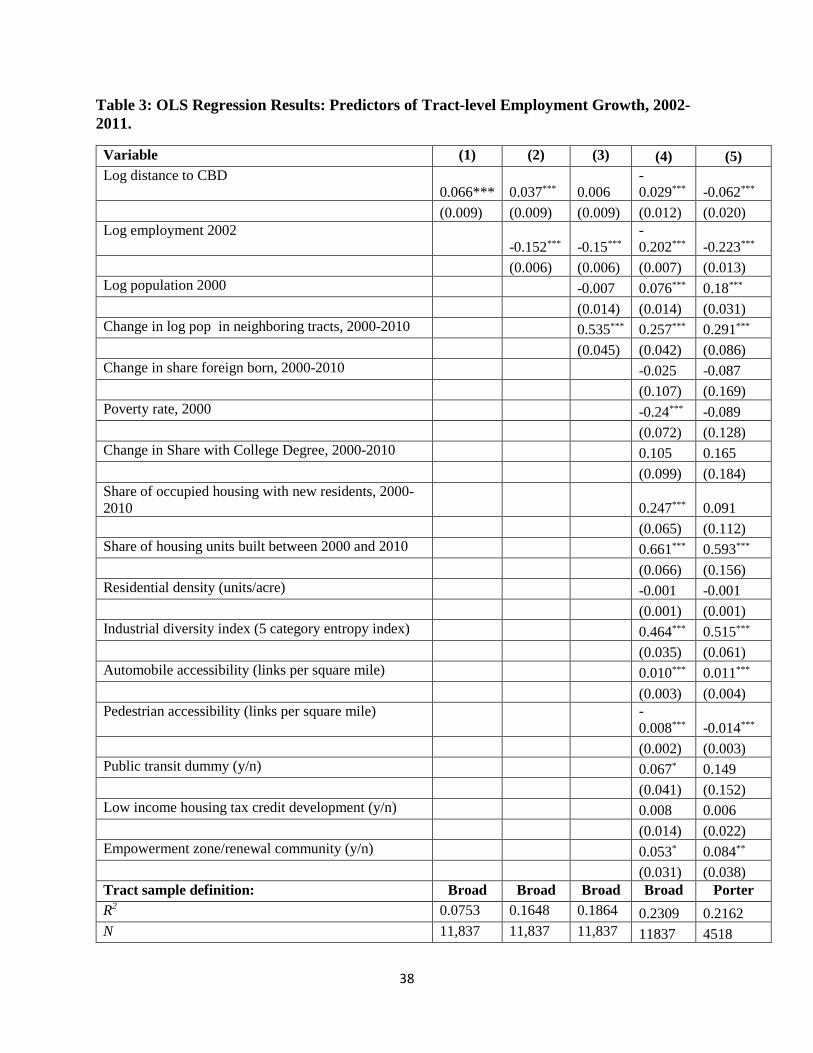
Table 3 presents our tract-level regression results aimed at revealing some of the

correlates of non-CBD inner-city-employment growth. The table shows four specifications, with

an increasing number of explanatory variables. The specification in column 1 includes the log of

the distance from the centroid of the tract to the CBD. The coefficient of 0.066 means that tracts

that are twice as far from the CBD have on average 4.6 more log points of employment growth

(0.69 * 0.066 = 0.046). The specification in column 2 adds the log of initial-year (2002)

employment. This variable is added to help mitigate potential measurement error problems in

the tract-level employment data. Adding this control reduces the magnitude of the coefficient on

the distance to CBD measure. Column 3 adds local demand variables in the form of the log of

25

the tracts’ own initial-year population and the change in the log of the population of all of the

tracts that share a border with the tract. In this specification, changes in the local area

(neighboring tract) population are correlated with tract-level employment growth. The

coefficient of 0.535 implies that, on average, a 10-log-point increase in neighboring tract

population is associated with a 5-log-point increase in own-tract employment.

[TABLE 3 ABOUT HERE]

The specification in column 4 contains our full set of tract-level explanatory variables.

The first thing that stands out is that the sign of the coefficient on the log of distance to CBD is

now negative and is not statistically different from zero. Conditional on all the other explanatory

variables, employment growth is negatively correlated with distance to the CBD. In other

words, controlling for other factors, neighborhoods closer to downtown-added jobs at a faster

rate than those further away, indicating the importance of proximity to the largest concentration

of employment in region. The log of initial year (2000) tract population is now positively related

to employment growth. The change in the log population of neighboring tracts is still positively

related to employment growth, but conditional on all the other explanatory variables the

coefficient has dropped to about half of its value in column 3. Higher poverty rate tracts are

associated with less employment growth. All else equal, a 10-percentage-point higher poverty

rate is associated with 2.4 fewer log points of employment growth. Thus, neighborhood poverty

still seems to be a deterrent to local employment growth.

The coefficient on the change in the share with a college degree is positive but not

statistically different from zero. Although we would expect that this would be an important

variable, given the literature on gentrification and then urban preferences of the creative class, it

26

is likely that the effect of this variable is usurped by the next two variables, which are also

indicators of residential changes. Specifically, the share of occupied housing units with

residents that moved in during the 2000s (an indicator or recent migration to the area) is

positively correlated with employment growth. This higher residential turnover is consistent

with urban re-development. Further evidence that employment growth and re-development are

correlated comes from the positive coefficient on the share of housing units built during the

2000s. It appears that tracts with a 10-percentage-point higher share of units built during the

2000s have, on average, 6.6 logs point higher employment growth. Finally, our measure of

immigration is not significant in any specification. This is interesting given the literature on

immigrant ethnic enclaves and business growth. While we cannot conclude that immigration

does not lead to job growth in some neighborhoods, our analysis suggests that other factors

outweigh the impact of recent immigration.

The coefficient on residential density is negative, though not statistically significant.

This is not surprising as tracts that have mostly residential uses (and thus higher density) have

little room left for commercial land uses and the jobs located therein. Industrial diversity –

measured as the five-category employment entropy index—is positively correlated with

employment growth over the period. Automobile accessibility shows a positive correlation with

employment growth, while pedestrian accessibility is negatively correlated with employment

growth. This makes sense given the local land-use conditions in most inner cities where areas

zoned for commercial or industrial activity lie along major arterial roadways (with high

automobile accessibility), while residential tracts—that may contain denser networks of smaller

streets—do not have as much room for employment growth. Finally, there is a statistically

significant association between the presence of a public transit stop and employment growth.

27

The coefficient implies that tracts containing public transit stops saw roughly 6.7 log points

higher employment growth than those without a public transit stop.

There is no clear association between the presence of low-income-housing-tax-credit

developments and employment growth. There is a marginally, statistically significant, positive

relationship between empowerment zone (EZ)/renewal community (RC) status and employment

growth. Whereas we do not consider this strong causal evidence of the effectiveness of EZ/RC

policies, it is consistent with the findings of recent research (Busso, Gregory, & Kline, 2010) .

On average, tracts in these programs saw about 5.3 log points higher employment growth than

other inner-city tracts.

The specification in column 4 has an R-squared of 0.23, meaning that our full set of

explanatory variables can explain about a quarter of the variation in tract-level employment

growth. In specifications without the city fixed effect (not shown), the R-squared drops to 0.19,

and without the log of initial-year employment, it drops to 0.12. The R-squared drops slightly in

our model using the narrower, Porter inner-city definition (0.21) shown in column 5.

Column 5 presents estimates of the same specification as column 4, but the sample is

limited to the set of economically distressed inner-city tracts that meet the Porter definition of

having a median household income lower than 80% of that of the MSA and an unemployment

rate greater than 1.25 times the MSA average in 2000. Most of the estimates in column 5 are

similar to those shown in column 4 for the broadly defined sample of inner city tracts. There are

six main differences. First, we observe an increased conditional correlation between

employment growth and proximity to the CBD; the coefficient roughly doubles in magnitude.

Second, there is an increased conditional correlation between year 2000 population. Third, we

28

see a decreased conditional correlation with the poverty rate. This makes sense, as there is less

variation in poverty rates across the tracts in the Porter definition as it selects on lower income

status. This means that among these distressed tracts, variation in the poverty rate is less

predictive of employment growth than among the full sample. Fourth, there is less of a

conditional correlation between the change in the share of occupied housing with new residents,

possibly indicating less of an association between gentrification and employment growth among

distressed tracts. Fifth, the relationship between pedestrian accessibility and employment growth

appears to be slightly more negative. Sixth, we observe an increased conditional correlation

between employment growth and EZ/RC status. Thus among distressed tracts, EZ/RC status is

associated with 8.4 log points higher employment growth than other distressed inner-city tracts.

Conclusion

For America’s inner cities as a whole, the decade of the 2000s stands in stark relief

compared to the 1980s and 1990s in terms of job growth. Using a data set that was unavailable

in the past (LODES), we show that inner-city tracts (those in the non-CBD portions of the large

central cities) added 1.8 million jobs between 2002 and 2011. This trend is not just limited to a

few cities and regions, as inner-city growth was positive in nearly all census divisions and even

outpaced suburban growth rates in some areas. The post-recession period has been even stronger

for inner cities. Although the overall national trend is encouraging given the scale of job losses

in previous decades, this growth is probably not enough to declare a “renaissance” in urban

America.

When we compare job growth between all inner-city tracts and only those inner-city tracts

that exhibited higher levels of economic distress (i.e., Porter’s method), some interesting facts

29

emerge. First, the positive growth trend is still evident but is less pronounced. This means that

distressed inner-city areas still face significant barriers, compared to similarly located but less

distressed urban neighborhoods. As our tract-level models indicate, these highly distressed areas

are less likely to receive the positive effects of gentrification (i.e., increased local service sector

jobs) and that the job growth that has occurred in these areas is tied to different drivers (as we

discuss below).

Turning to the question of competitiveness, regional growth differentials are clearly

important, as the literature on city-suburban dependence indicates. It is not surprising that New

York City and San Francisco have much higher inner-city-employment growth, as they are

located within strong, growing metropolitan areas. However, in places like Dallas and Houston,

which also grew, suburban employment continues to outpace inner-city employment, suggesting

important differences in characteristics and policies of the metropolitan areas that result in

competitive inner cities. Yet, places known for their suburban dominance such as Los Angeles

and San Antonio showed strong inner city resurgence in the last decade. Thus competitive inner

cities emerged in some unlikely places. We find that, although competitive inner cities are no

longer the exception, they are also not universal. Two fifths (144 out of 281) of the metros

studied in this analysis have seen both increases in overall employment increases in share of

inner-city employment. Much of the growth in these metropolitan areas is driven by growth in

the high wage sectors.

There are also important differences in the nature of job growth by sector. The inner city

resurgence has been led by the so-called “eds and meds” of Health Care and Educational

Services; at the same time losses in manufacturing and construction jobs continue in the inner

city, reflecting the twin trends of globalization and suburbanization of manufacturing. Within

30

inner cities, access to physical infrastructure (e.g., proximity to the CBD, transit), as well as

social infrastructure (e.g., population increases nearby) confer significant advantages for job

growth. However, if access to infrastructure is one of the competitive strengths of the inner

cities, it is not reflected in the job growth in the sectors that largely depend on infrastructure

(such as manufacturing). Instead, the job growth is driven by residentiary sectors such as food

services, supporting some claims from the gentrification literature that inner-city job growth is

fueled at least in part by recent residential growth. Yet for distressed inner-city areas, job

growth is driven less by local consumption but rather by growth in anchor institutions that make

up the “eds and meds” sector (see Figure 3).

However, our findings also indicate that inner-city job growth tends to be greater in areas

that are relatively less poor. Thus high poverty neighborhoods still seem to have major barriers

that limit more robust employment gains. It is here that there may be a continued role for

government intervention. Our finding that either tracts designated as an empowerment zone or

renewal community grew faster, on average, than other tracts, suggests that economic

development strategies that are targeted to high poverty areas can play a role. Our results

suggest that, overall, inner-city areas do have real advantages as locations for employment and

are increasingly viewed as attractive residential locations.

31

(Bates; Harrison & Glasmeler)

References

Abowd, J. M., Stephens, B. E., Vilhuber, L., Andersson, F., McKinney, K. L., Roemer, M., &

Woodcock, S. (2009). The LEHD infrastructure files and the creation of the Quarterly

Workforce Indicators Producer Dynamics: New Evidence from Micro Data (pp. 149-

230): University of Chicago Press.

Adams, C. (2003). The meds and eds in urban economic development. Journal of Urban Affairs,

25(5), 571-588.

Aliprantis, D., Fee, K., & Oliver, N. (2014). Which Poor Neighborhoods Experienced Income

Growth in Recent Decades? Cleveland: Federal Reserve Bank of Cleveland.

Bates, T. (1997a). Financing small business creation: the case of Chinese and Korean immigrant

entrepreneurs. Journal of business venturing, 12(2), 109-124.

Bates, T. (1997b). Response: Michael Porter's Conservative Urban Agenda will not Revitalize

America's Inner Cities: What will? Economic Development Quarterly, 11(1), 39-44. doi:

10.1177/089124249701100104

Bates, T. (2011). Minority entrepreneurship. Foundations and Trends in Entrepreneurship, 7(3-

4).

Bivand, R. (2015). Spatial Dependence: Weighting Schemes, Statistics and Models. R package

(spdep) (Version version 0.5-81). Retrieved from http://CRAN.R-

project.org/package=spdep

Busso, M., Gregory, J., & Kline, P. M. (2010). Assessing the incidence and efficiency of a

prominent place based policy: National Bureau of Economic Research.

Chapple, K. (2006). Connection missed: Revisiting the spatial mismatch hypothesis in the new

metropolitan reality. Journal of the American Planning Association, forthcoming.

Clark, J. (2013). Working Regions: Reconnecting Innovation and Production in the Knowledge

Economy: Routledge.

Cortright, J., & Mahmoudi, D. (2014). Neighborhood Change, 1970 to 2010: Transition and

Growth in Urban High Poverty Neighborhoods (pp. 22). Portland, OR: Impresa

Economics.

Csardi, G., & Nepusz, T. (2006). The igraph software package for complex network research.

InterJournal, Complex Systems, 1695.

32

Curran, W. (2004). Gentrification and the nature of work: exploring the links in Williamsburg,

Brooklyn. Environment and Planning A, 36(7), 1243-1258. doi: doi:10.1068/a36240

Curran, W. (2007). 'From the Frying Pan to the Oven': Gentrification and the Experience of

Industrial Displacement in Williamsburg, Brooklyn. Urban Studies, 44(8), 1427-1440.

doi: 10.1080/00420980701373438

Fee, K., & Hartley, D. (2011). Urban Growth and Decline: The Role of Population Density at the

City Core.

Florida, R. (2003). Cities and the Creative Class. City & Community, 2(1), 3-19. doi:

10.1111/1540-6040.00034

Florida, R. L. (2002). The rise of the creative class : and how it's transforming work, leisure,

community and everyday life. New York, NY: Basic Books.

Freeman, L. (2005). Displacement or Succession? Urban Affairs Review, 40(4), 463-491. doi:

10.1177/1078087404273341

Galster, G. C., & Killen, S. P. (1995). The geography of metropolitan opportunity: a

reconnaissance and conceptual framework. Housing Policy Debate, 6(1), 7-43.

Garcia-López, M.-À. (2010). Population suburbanization in Barcelona, 1991–2005: Is its spatial

structure changing? Journal of Housing Economics, 19(2), 119-132.

Graham, M. R., Kutzbach, M. J., & McKenzie, B. (2014). Design Comparison Of Lodes And

Acs Commuting Data Products.

Harkavy, I. R., & Zuckerman, H. (1999). Eds and meds: Cities' hidden assets: Brookings

Institution, Center on Urban and Metropolitan Policy.

Harrison, B., & Glasmeler, A. K. (1997). Response: Why Business Alone won't Redevelop the

Inner City: A Friendly Critique of Michael Porter's Approach to Urban Revitalization.

Economic Development Quarterly, 11(1), 28-38. doi: 10.1177/089124249701100103

Hill, E. W., Wolman, H. L., & Ford, C. C. (1995). Can suburbs survive without their central

cities? Examining the suburban dependence hypothesis. Urban Affairs Review, 31(2),

147-174.

Hutton, T. A. (2004). The new economy of the inner city. Cities, 21(2), 89-108.

Ihlanfeldt, K., & Sjoquist, D. (1989). The impact of job decentralization on the economic welfare

of central-city blacks. Journal of Urban Economics, 26, 110-130 .

33

Kain, J. (1968). Housing segregation, Negro employment, and metropolitan decentralization.

Quarterly Journal of Economics, 82(2), 175�197

Kasarda, J. D. (1993). Inner‐city concentrated poverty and neighborhood distress: 1970 to 1990.

Housing Policy Debate, 4(3), 253-302.

Katz, M. B. (1993). The" underclass" debate: Views from history: Princeton University Press.

Ledebur, L. C., & Barnes, W. R. (1993). "All in it Together": Cities, Suburbs, and Local

Economic Regions. Resarch Report on America's Cities. Washington D.C.: National

League of Cities.

Lester, T. W., & Hartley, D. A. (2014). The long term employment impacts of gentrification in

the 1990s. Regional Science and Urban Economics, 45(0), 80-89. doi:

http://dx.doi.org/10.1016/j.regsciurbeco.2014.01.003

Ley, D. (1996). The new middle class and the remaking of the central city Oxford University

Press: Oxford.

Lloyd, R., & Clark, T. N. (2001). The city as an entertainment machine. In K. Fox Gotham (Ed.),

Critical Perspectives on Urban Redevelopment (pp. 357-378): Emerald Group Publishing

Limited.

Marcuse, P. (1985). Gentrification, abandonment, and displacement: Connections, causes, and

policy responses in New York City. Washington University journal of urban and

contemporary law, 28(Journal Article), 195. doi: pmid:

McMillen, D. P. (2001). Nonparametric employment subcenter identification. Journal of Urban

Economics, 50(3), 448-473.

McMillen, D. P. (2003). Identifying sub-centres using contiguity matrices. Urban Studies, 40(1),

57-69.

Meltzer, R., & Schuetz, J. (2012). Bodegas or Bagel Shops? Neighborhood Differences in Retail

and Household Services. Economic Development Quarterly, 26(1), 73-94. doi:

10.1177/0891242411430328

Moretti, E. (2012). The New Geography of Jobs. New York: Houghton Mifflin Harcourt.

Owen, A., & Levinson, D. M. (2015). Modeling the commute mode share of transit using

continuous accessibility to jobs. Transportation Research Part A: Policy and Practice,

74, 110-122.

34

Pack, J. R. (2002). Growth and convergence in metropolitan America. Washington, D.C.:

Brookings Institution Press.

Pastor, M., Drier, P., & al., e. (2000). Regions that Work: How Cities and Suburbs Can Grow

Together. Minneapolis: University of Minnesota.

Pastor, M., Lester, T. W., & Scoggins, J. (2009). WHY REGIONS? WHY NOW? WHO

CARES? Journal of Urban Affairs, 31(3), 269-296. doi: 10.1111/j.1467-

9906.2009.00460.x

Pastor, M., Scoggins, J., Lester, T. W., & Chapple, K. (2009). Building Resilient Regions

Database [Machine-readable databse]: A Project of the John D. and Catherine T.

MacArthur Foundation.

Portes, A., & Zhou, M. (1992). Gaining the upper hand: Economic mobility among immigrant

and domestic minorities. Ethnic and racial studies, 15(4), 491-522.

Sampson, R. J. (2008). Rethinking crime and immigration. Contexts, 7(1), 28-33.

Saxenian, A. (1994). Regional advantage : culture and competition in Silicon Valley and Route

128. Cambridge, Mass.: Harvard University Press.

Schleith, D., & Horner, M. (2014). Commuting, Job Clusters, and Travel Burdens: Analysis of

Spatially and Socioeconomically Disaggregated Longitudinal Employer-Household

Dynamics Data. Transportation Research Record: Journal of the Transportation

Research Board(2452), 19-27.

Smith, N. (1996). The New Urban Frontier: Gentrification and the Revanchist City. London:

Routledge.

Smith, N. (2002). New Globalism, New Urbanism: Gentrification as Global Urban Strategy.

Antipode, 34(3), 427-450. doi: 10.1111/1467-8330.00249

Sohmer, R. R., & Lang, R. E. (2001). Downtown rebound. Redefining Urban and Suburban

America: Evidence From Census 2000, 1, 63-74.

Storper, M. (1997). The Regional World: Territorial Development in a Global Economy. New

York: Guilford.

Suárez, M., & Delgado, J. (2009). Is Mexico City Polycentric? A trip attraction capacity

approach. Urban Studies, 46(10), 2187-2211.

Teitz, M., & Chapple, K. (1998). The causes of inner-city poverty: Eight hypotheses in search of

reality. Citiscape: A Journal of Policy Development and Research, 3(3), 33-70.

35

Vigdor, J. L. (2002). Does Gentrification Harm the Poor? [with Comments]. Brookings-Wharton

papers on urban affairs(ArticleType: research-article / Full publication date: 2002 /

Copyright © 2002 Brookings Institution Press), 133-182.

Voith, R. (1992 ). City and Suburban Growth: Substitutes or Compliments. Business Review-

Federal Reserve Bank of Philadelphia, September-October, 21-33.

Voith, R. (1998). Do suburbs need cities? Journal of Regional Science, 38(3), 445-464.

Wilson, W. J. (1987). The truly disadvantaged : the inner city, the underclass, and public policy.

Chicago: University of Chicago Press.

Wilson, W. J. (1996). When work disappears : the world of the new urban poor (1st ed.). New

York: Knopf : Distributed by Random House, Inc.

Wyly, E. K., & Hammel, D. J. (1999). Islands of decay in seas of renewal: Housing policy and

the resurgence of gentrification. Housing Policy Debate, 10(4), 711-771. doi:

10.1080/10511482.1999.9521348

Zukin, S. (1982). Loft living : culture and capital in urban change. Baltimore: Johns Hopkins

University Press.

36

Table 1. Employment Change in CBD, Inner City, Suburban, and Nonmetro tracts, 2002-11.

Year CBD Inner city Inner city- Porter

Suburban Nonmetro Total

Total employment 2002 9,806,579 29,699,043 9,163,969 59,207,009 15,401,902 114,114,533 2003 9,466,413 29,406,696 8,959,707 59,122,731 15,351,324 113,347,164 2004 9,368,606 29,688,362 9,040,566 60,114,666 15,481,987 114,653,621 2005 9,391,107 30,143,171 9,140,514 61,722,807 15,711,700 116,968,785 2006 9,502,148 30,512,600 9,137,376 62,976,328 15,969,935 118,961,011 2007 9,462,838 31,030,945 9,279,914 64,129,684 16,113,194 120,736,661 2008 9,422,301 31,082,578 9,181,937 64,323,119 16,120,592 120,948,590 2009 9,405,450 30,425,117 9,025,946 61,460,391 15,426,231 116,717,189 2010 9,599,146 30,796,523 9,175,827 61,733,541 15,466,790 117,596,000 2011 9,654,338 31,521,499 9,292,356 63,296,946 15,758,332 120,231,115

Net employment change (2002-11)

(152,241) 1,822,456 128,387 4,089,937 356,430 6,116,582

% change -1.6% 6.1% 1.4% 6.9% 2.3% 5.4% Post-Recession net change (2009-11)

248,888 1,096,382 266,410 1,836,555 332,101 3,513,926

% change 2.6% 3.6% 3.0% 3.0% 2.2% 3.0% Share of U.S. employment, 2002 8.6% 26.0% 8.0% 18.4% 51.9%

Share of U.S. employment, 2011 8.0% 26.2% 7.7% 18.2% 52.6%

Note: Authors analysis of Local Origin-Destination Employment Statistics (LODES) data by tract type for states with full sample (2002-11).

37

Table 2. Inner-city Employment Change by Tract Poverty Status.

Tract poverty status, 1990 Tract poverty status, 2000 Employment measure Low poverty

(<20%) High

poverty (>20%)

Extreme poverty (>40%)

Low poverty (<20%)

High poverty >20%

Extreme poverty (>40%)

Total employment, 2002 19,843,121 9,855,922 2,879,470 19,779,094 9,919,949 2,177,597 % of inner-city jobs, 2011 66.8% 33.2% 9.7% 66.6% 33.4% 7.3% Total employment, 2009 20,581,454 9,843,663 2,936,604 20,440,333 9,984,784 2,206,598 % of inner-city jobs, 2011 67.6% 32.4% 9.7% 67.2% 32.8% 7.3% Total employment, 2011 21,296,609 10,224,890 3,183,065 21,116,880 10,404,619 2,352,930 % of inner-city jobs, 2011 67.6% 32.4% 10.1% 67.0% 33.0% 7.5% Net employment change (2002-11)

1,453,488 368,968 303,595 1,337,786 484,670 175,333

% change 7.3% 3.7% 10.5% 6.8% 4.9% 8.1% Net employment change (2009-11)

715,155 381,227 246,461 676,547 419,835 146,332

% change 3.5% 3.9% 8.4% 3.3% 4.2% 6.6% Source: Authors analysis of Local Origin-Destination Employment Statistics (LODES) data, 2002-2011.

38

Table 3: OLS Regression Results: Predictors of Tract-level Employment Growth, 2002-2011.

Variable (1) (2) (3) (4) (5) Log distance to CBD

0.066*** 0.037*** 0.006 -0.029*** -0.062***

(0.009) (0.009) (0.009) (0.012) (0.020) Log employment 2002

-0.152*** -0.15*** -0.202*** -0.223***

(0.006) (0.006) (0.007) (0.013) Log population 2000 -0.007 0.076*** 0.18*** (0.014) (0.014) (0.031) Change in log pop in neighboring tracts, 2000-2010 0.535*** 0.257*** 0.291*** (0.045) (0.042) (0.086) Change in share foreign born, 2000-2010 -0.025 -0.087 (0.107) (0.169) Poverty rate, 2000 -0.24*** -0.089 (0.072) (0.128) Change in Share with College Degree, 2000-2010 0.105 0.165 (0.099) (0.184) Share of occupied housing with new residents, 2000-2010

0.247*** 0.091

(0.065) (0.112) Share of housing units built between 2000 and 2010 0.661*** 0.593*** (0.066) (0.156) Residential density (units/acre) -0.001 -0.001 (0.001) (0.001) Industrial diversity index (5 category entropy index) 0.464*** 0.515*** (0.035) (0.061) Automobile accessibility (links per square mile) 0.010*** 0.011*** (0.003) (0.004) Pedestrian accessibility (links per square mile) -

0.008*** -0.014*** (0.002) (0.003) Public transit dummy (y/n) 0.067* 0.149 (0.041) (0.152) Low income housing tax credit development (y/n) 0.008 0.006 (0.014) (0.022) Empowerment zone/renewal community (y/n) 0.053* 0.084** (0.031) (0.038) Tract sample definition: Broad Broad Broad Broad Porter R2 0.0753 0.1648 0.1864 0.2309 0.2162 N 11,837 11,837 11,837 11837 4518

39

Note: Robust standard errors in parentheses below estimate. *Significant at 10%. **Significant at 5%. ***Significant at 1%.

40

Figure1. Delineation of Inner-city Status in the Cleveland, MSA.

41

Figure 1. Employment Change by Tract Type and Census Division, Full Period and Post-Recession.

‐10.0%

‐5.0%

0.0%

5.0%

10.0%

15.0%

20.0%

25.0%

30.0%Em

ploy

men

t Gro

wth

(200

2-20

11)

Census Division

CBD

Inner City

Suburban

42

Figure 3. Inner-City Employment Change by Major Industry Sector (NAICS), Full Period (2002-11) and Post Recession (2009-11).

‐3.0%

‐2.0%

‐1.0%

0.0%

1.0%

2.0%

3.0%

4.0%

5.0%

6.0%

7.0%Em

ploy

men

t Gro

wth

, 200

9-20

11

Census Division

CBD

Inner‐city

Suburban

43

Source: Authors analysis of Local Origin-Destination Employment Statistics (LODES) data, 2002-2011.

(1,000,000) (500,000) ‐ 500,000 1,000,000 1,500,000

Health Care and Social Assistance (62)

Educational Srvs. (61)

Accommodation and Food Srvs. (72)

Professional and Technical Srvs. (54)

Public Administration (92)

Finance and Insurance (52)

Other Services (81)

Management of Companies and Ent. (55)

Administrative and Support Srvs. (56)

Arts, Entertainment, and Recreation (71)

Mining and Extraction (21)

Transportation and Warehousing (48‐49)

Agriculture (11)

Utilities (22)

Real Estate and Rental and Leasing (53)

Retail Trade (44‐45)

Information (51)

Wholesale Trade (42)

Construction (23)

Manufacturing (31‐33)

Net Employment Change

Full Period(2002‐11)

Post‐Recession(2009‐11)

44

Figure 4. Defining Inner-city Competitiveness: MSA Employment Change and the Change in Inner-city Proportion of Employment in 2002 and 2011.

Source: Authors analysis of Local Origin-Destination Employment Statistics (LODES) data, 2002-2011.

45

46

Figure 5. Characteristics of Metropolitan Regions with Competitive Inner Cities (Broad Definition) Versus All Other Metros.

Notes: Figure presents the difference in distribution of various indicators for metropolitan areas with competitive inner cities and to the distribution for all other metropolitan areas.

Sources: LODES (panel 1-3), Building Resilient Regions (BRR) database (panels 4-8), U.S. Environmental Protection Agency (EPA) Smart Location database (panels 9-11). All variables calculated at the metropolitan core-based statistical area (CBSA) level. N=281.

47

Figure 6. Regions with Competitive Inner Cities, Using Different Definitions.

A. Appendix: List of Regions with Competitive Inner Cities.

Share of employment in the inner city (Porter)

Share of employment in the inner city

(broad)

Difference in shares

Difference in shares

CBSA name 2002 2011 2002 2011

Competitive inner-city regions in both definitions Ames, IA 0.034 0.221 0.186 0.109 0.305 0.196 Athens-Clarke County, GA 0.084 0.248 0.164 0.569 0.726 0.156 Blacksburg-Christiansburg-Radford, VA 0.011 0.160 0.149 0.063 0.213 0.150 Morgantown, WV 0.085 0.212 0.127 0.145 0.273 0.128 Lawrence, KS 0.045 0.067 0.022 0.468 0.593 0.125 Columbia, MO 0.168 0.173 0.005 0.492 0.602 0.111 Jackson, TN 0.036 0.047 0.011 0.573 0.681 0.108 Bowling Green, KY 0.140 0.185 0.045 0.629 0.698 0.069 Jackson, MI 0.069 0.136 0.067 0.210 0.274 0.064 Chattanooga, TN-GA 0.185 0.224 0.039 0.523 0.580 0.057 Springfield, IL 0.167 0.189 0.022 0.473 0.529 0.056 Springfield, OH 0.126 0.173 0.047 0.392 0.448 0.056 Atlantic City, NJ 0.057 0.080 0.024 0.077 0.133 0.056 Sumter, SC 0.039 0.046 0.007 0.220 0.275 0.055 Anchorage, AK 0.335 0.347 0.012 0.807 0.860 0.053 New Haven-Milford, CT 0.086 0.090 0.004 0.104 0.156 0.052 Salinas, CA 0.027 0.064 0.037 0.101 0.142 0.041 Lexington-Fayette, KY 0.142 0.203 0.061 0.614 0.652 0.038 New York-Northern New Jersey-Long Island, NY-NJ-PA 0.074 0.084 0.010 0.368 0.403 0.035 Sacramento--Arden-Arcade--Roseville, CA 0.082 0.100 0.018 0.195 0.229 0.035

49

Oshkosh-Neenah, WI 0.067 0.147 0.080 0.291 0.325 0.034 Longview, WA 0.012 0.015 0.003 0.048 0.082 0.033 Bakersfield, CA 0.052 0.052 0.001 0.316 0.348 0.033 Gadsden, AL 0.180 0.198 0.018 0.380 0.411 0.031 Florence, SC 0.017 0.021 0.004 0.095 0.125 0.030 Salem, OR 0.272 0.286 0.014 0.364 0.393 0.029 Corvallis, OR 0.211 0.223 0.012 0.373 0.401 0.028 Merced, CA 0.064 0.085 0.021 0.177 0.203 0.026 Cleveland-Elyria-Mentor, OH 0.099 0.126 0.027 0.146 0.171 0.025 Myrtle Beach-Conway-North Myrtle Beach, SC 0.088 0.091 0.003 0.320 0.344 0.024 Chico, CA 0.001 0.001 0.000 0.165 0.188 0.023 Rome, GA 0.050 0.057 0.007 0.253 0.276 0.023 Florence-Muscle Shoals, AL 0.021 0.021 0.000 0.323 0.345 0.022 San Jose-Sunnyvale-Santa Clara, CA 0.107 0.120 0.013 0.371 0.392 0.020 Auburn-Opelika, AL 0.121 0.132 0.011 0.294 0.314 0.020 Parkersburg-Marietta, WV-OH 0.021 0.047 0.026 0.167 0.187 0.020 Durham, NC 0.123 0.169 0.046 0.396 0.414 0.019 Utica-Rome, NY 0.091 0.107 0.016 0.213 0.231 0.018 Oxnard-Thousand Oaks-Ventura, CA 0.028 0.036 0.008 0.314 0.332 0.018 Spartanburg, SC 0.026 0.044 0.018 0.095 0.111 0.016 Rochester, MN 0.051 0.052 0.001 0.498 0.513 0.015 Duluth, MN-WI 0.008 0.010 0.002 0.275 0.290 0.015 Longview, TX 0.070 0.093 0.023 0.294 0.308 0.014 Palm Bay-Melbourne-Titusville, FL 0.107 0.127 0.020 0.304 0.318 0.014 Los Angeles-Long Beach-Santa Ana, CA 0.061 0.067 0.006 0.231 0.244 0.013 Fort Collins-Loveland, CO 0.030 0.037 0.006 0.339 0.352 0.012 Abilene, TX 0.113 0.122 0.009 0.583 0.594 0.011 Valdosta, GA 0.097 0.120 0.023 0.343 0.353 0.010 Columbus, GA-AL 0.120 0.125 0.005 0.642 0.652 0.010 Lakeland, FL 0.030 0.051 0.021 0.197 0.206 0.009

50

Pittsburgh, PA 0.046 0.057 0.011 0.107 0.115 0.008 Fayetteville, NC 0.075 0.084 0.010 0.624 0.632 0.008 State College, PA 0.041 0.049 0.009 0.098 0.104 0.007 Fairbanks, AK 0.142 0.155 0.014 0.224 0.230 0.006 Las Cruces, NM 0.038 0.039 0.001 0.368 0.374 0.006 Asheville, NC 0.070 0.073 0.002 0.289 0.295 0.006 Monroe, LA 0.069 0.082 0.013 0.155 0.159 0.004 Scranton--Wilkes-Barre, PA 0.009 0.012 0.004 0.090 0.094 0.004 Charleston-North Charleston, SC 0.034 0.035 0.001 0.165 0.168 0.002 Philadelphia-Camden-Wilmington, PA-NJ-DE-MD 0.070 0.070 0.000 0.142 0.143 0.001 San Diego-Carlsbad-San Marcos, CA 0.079 0.089 0.010 0.500 0.501 0.000

Additional competitive inner-city regions (using Porter definition) Albany-Schenectady-Troy, NY 0.077 0.094 0.017 0.252 0.247 -0.005 Alexandria, LA 0.043 0.046 0.002 0.271 0.270 -0.001 Altoona, PA 0.045 0.054 0.009 0.370 0.309 -0.061 Atlanta-Sandy Springs-Marietta, GA 0.037 0.039 0.002 0.107 0.106 -0.001 Bloomington, IN 0.052 0.054 0.002 0.276 0.267 -0.009 Bremerton-Silverdale, WA 0.039 0.039 0.000 0.153 0.133 -0.019 Cumberland, MD-WV 0.021 0.022 0.001 0.206 0.190 -0.016 Grand Forks, ND-MN 0.062 0.070 0.008 0.432 0.427 -0.005 Grand Rapids-Wyoming, MI 0.059 0.069 0.010 0.206 0.195 -0.011 Greenville, NC 0.062 0.063 0.000 0.409 0.405 -0.004 Harrisonburg, VA 0.057 0.122 0.065 0.515 0.445 -0.070 Honolulu, HI 0.167 0.170 0.002 0.585 0.554 -0.032 Kalamazoo-Portage, MI 0.056 0.091 0.035 0.361 0.329 -0.032 Killeen-Temple-Fort Hood, TX 0.056 0.131 0.075 0.599 0.585 -0.014 Lancaster, PA 0.032 0.037 0.005 0.117 0.116 -0.001 Lubbock, TX 0.245 0.250 0.006 0.782 0.775 -0.008

51

Madison, WI 0.174 0.220 0.047 0.572 0.522 -0.050 Norwich-New London, CT 0.025 0.028 0.002 0.122 0.121 -0.001 Ocala, FL 0.013 0.016 0.003 0.293 0.284 -0.009 Ogden-Clearfield, UT 0.038 0.049 0.011 0.106 0.098 -0.008 Pueblo, CO 0.157 0.186 0.029 0.484 0.450 -0.034 Santa Barbara-Santa Maria-Goleta, CA 0.035 0.035 0.001 0.430 0.424 -0.007 Visalia-Porterville, CA 0.004 0.006 0.002 0.256 0.251 -0.005 Waco, TX 0.122 0.143 0.021 0.463 0.420 -0.043

Additional competitive inner-city regions (using broad definition) Albuquerque, NM 0.223 0.158 -0.065 0.732 0.734 0.002 Ann Arbor, MI 0.269 0.152 -0.118 0.483 0.542 0.059 Appleton, WI NA NA NA 0.250 0.340 0.090 Bellingham, WA 0.052 0.045 -0.007 0.321 0.338 0.017 Bend, OR NA NA NA 0.287 0.316 0.029 Bismarck, ND NA NA NA 0.300 0.373 0.074 Bloomington-Normal, IL NA NA NA 0.512 0.527 0.015 Brownsville-Harlingen, TX 0.076 0.075 -0.002 0.413 0.439 0.026 Cape Coral-Fort Myers, FL NA NA NA 0.086 0.090 0.004 Clarksville, TN-KY 0.085 0.085 0.000 0.359 0.419 0.061 College Station-Bryan, TX 0.015 0.013 -0.002 0.183 0.226 0.043 Colorado Springs, CO 0.177 0.137 -0.040 0.697 0.698 0.001 Columbia, SC 0.033 0.030 -0.003 0.182 0.190 0.008 Corpus Christi, TX 0.212 0.208 -0.005 0.580 0.605 0.025 Davenport-Moline-Rock Island, IA-IL 0.093 0.085 -0.009 0.304 0.323 0.019 Dubuque, IA 0.025 0.021 -0.004 0.445 0.466 0.021 Glens Falls, NY NA NA NA 0.046 0.105 0.058 Goldsboro, NC 0.161 0.149 -0.012 0.407 0.441 0.034 Jacksonville, FL 0.178 0.155 -0.023 0.628 0.637 0.009 Johnson City, TN NA NA NA 0.338 0.405 0.066

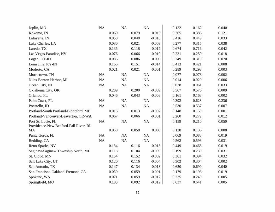
52

Joplin, MO NA NA NA 0.122 0.162 0.040 Kokomo, IN 0.060 0.079 0.019 0.265 0.386 0.121 Lafayette, IN 0.058 0.048 -0.010 0.416 0.449 0.033 Lake Charles, LA 0.030 0.021 -0.009 0.277 0.315 0.038 Laredo, TX 0.135 0.118 -0.017 0.674 0.716 0.042 Las Vegas-Paradise, NV 0.076 0.066 -0.010 0.231 0.250 0.018 Logan, UT-ID 0.086 0.086 0.000 0.249 0.319 0.070 Louisville, KY-IN 0.165 0.151 -0.014 0.413 0.421 0.008 Modesto, CA 0.021 0.021 -0.001 0.289 0.293 0.003 Morristown, TN NA NA NA 0.077 0.078 0.002 Niles-Benton Harbor, MI NA NA NA 0.014 0.020 0.006 Ocean City, NJ NA NA NA 0.028 0.061 0.033 Oklahoma City, OK 0.209 0.200 -0.009 0.567 0.576 0.009 Orlando, FL 0.046 0.043 -0.003 0.161 0.163 0.002 Palm Coast, FL NA NA NA 0.392 0.628 0.236 Pocatello, ID NA NA NA 0.530 0.537 0.007 Portland-South Portland-Biddeford, ME 0.015 0.013 -0.002 0.148 0.150 0.001 Portland-Vancouver-Beaverton, OR-WA 0.067 0.066 -0.001 0.260 0.272 0.012 Port St. Lucie, FL NA NA NA 0.159 0.210 0.050 Providence-New Bedford-Fall River, RI-MA 0.058 0.058 0.000 0.128 0.136 0.008 Punta Gorda, FL NA NA NA 0.069 0.088 0.019 Redding, CA NA NA NA 0.562 0.593 0.031 Reno-Sparks, NV 0.134 0.116 -0.018 0.449 0.468 0.019 Saginaw-Saginaw Township North, MI 0.113 0.104 -0.009 0.199 0.230 0.031 St. Cloud, MN 0.154 0.152 -0.002 0.361 0.394 0.032 Salt Lake City, UT 0.120 0.116 -0.004 0.302 0.304 0.002 San Antonio, TX 0.147 0.134 -0.013 0.650 0.690 0.040 San Francisco-Oakland-Fremont, CA 0.059 0.059 -0.001 0.179 0.198 0.019 Spokane, WA 0.071 0.059 -0.012 0.235 0.240 0.005 Springfield, MO 0.103 0.092 -0.012 0.637 0.641 0.005

53

Tuscaloosa, AL 0.202 0.188 -0.014 0.446 0.459 0.013 Tyler, TX 0.064 0.063 -0.002 0.449 0.452 0.003 Vineland-Millville-Bridgeton, NJ NA NA NA 0.340 0.371 0.031 Warner Robins, GA 0.065 0.063 -0.002 0.240 0.269 0.030 Wenatchee, WA NA NA NA 0.159 0.165 0.005 Wilmington, NC 0.106 0.087 -0.019 0.443 0.448 0.004 Winston-Salem, NC 0.105 0.102 -0.003 0.600 0.612 0.012 Yakima, WA 0.051 0.048 -0.004 0.237 0.243 0.006 Yuba City, CA 0.044 0.036 -0.008 0.229 0.239 0.010

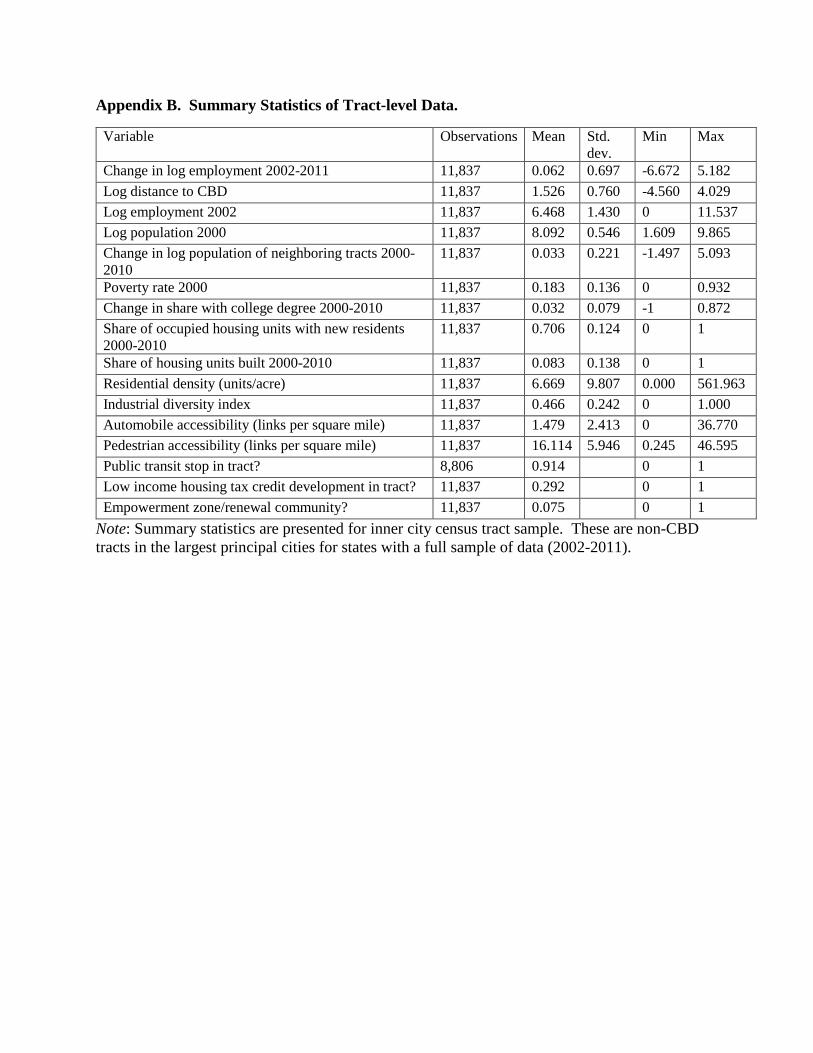
Appendix B. Summary Statistics of Tract-level Data.

Variable Observations Mean Std. dev.

Min Max

Change in log employment 2002-2011 11,837 0.062 0.697 -6.672 5.182 Log distance to CBD 11,837 1.526 0.760 -4.560 4.029 Log employment 2002 11,837 6.468 1.430 0 11.537 Log population 2000 11,837 8.092 0.546 1.609 9.865 Change in log population of neighboring tracts 2000-2010

11,837 0.033 0.221 -1.497 5.093

Poverty rate 2000 11,837 0.183 0.136 0 0.932 Change in share with college degree 2000-2010 11,837 0.032 0.079 -1 0.872 Share of occupied housing units with new residents 2000-2010

11,837 0.706 0.124 0 1

Share of housing units built 2000-2010 11,837 0.083 0.138 0 1 Residential density (units/acre) 11,837 6.669 9.807 0.000 561.963 Industrial diversity index 11,837 0.466 0.242 0 1.000 Automobile accessibility (links per square mile) 11,837 1.479 2.413 0 36.770 Pedestrian accessibility (links per square mile) 11,837 16.114 5.946 0.245 46.595 Public transit stop in tract? 8,806 0.914 0 1 Low income housing tax credit development in tract? 11,837 0.292 0 1 Empowerment zone/renewal community? 11,837 0.075 0 1

Note: Summary statistics are presented for inner city census tract sample. These are non-CBD tracts in the largest principal cities for states with a full sample of data (2002-2011).

55

Appendix C. Characteristics of Metropolitan Regions with Competitive Inner Cities (Porter Definition) Versus All other Metros.

56

Notes: Figure presents the difference in distribution of various indicators for metropolitan areas with competitive inner cities and to the distribution for all other metropolitan areas.

Sources: LODES (panel 1-3), Building Resilient Regions (BRR) database (panels 4-8), EPA Smart Location database (panels 9-11). All variables calculated at the metropolitan CBSA level. N=252.

57

i Throughout this study, we use the terms region and metropolitan area interchangeably. ii It is important to note, however, that Porter’s work was criticized by other scholars at the time, including Harrison and Glasmeier (1997) and Bates (1997), who argue that his approach placed too much emphasis on businesses as the primary agents of inner‐city revitalization and ignores critical roles for government and nonprofits. iii Specifically, Abowd et. al. (2009) explain the noise‐inducing algorithm that the LEHD infrastructure files use, as follows: “First, every data item [establishment] is distorted by some minimum amount. Second, for a given workplace, the data are always distorted in the same direction (increased or decreased) by the same percentage amount in every period….Third, the statistical properties of this distortion are such that when the estimates are aggregated, the effects of the distortion cancel out for the vast majority of the estimates, preserving both cross‐sectional and time series analytical validity” (p.184). iv Principal cities are defined for each MSA by the U.S. Census Bureau as the largest city in the MSA. Additional cities may qualify to be a principal city, if it is a census‐designated place or incorporated place with more than 250,000 residents and 100,000 workers or a place whose employment exceeds the population and both are at least 10,000. v http://www.epa.gov/smartgrowth/smartlocationdatabase.htm vi For the list of tracts that were included in EZ/RCs see http://portal.hud.gov/hudportal/HUD?src=/program_offices/comm_planning/economicdevelopment/programs/. vii Low income housing tax credit (LIHTC) unit counts by census tract were constructed from data published by the U.S. Department of Housing and Urban Development (HUD) on http://lihtc.huduser.gov/.