arctic landscape dynamics: modern processes and
TRANSCRIPT

ARCTIC LANDSCAPE DYNAMICS: MODERN PROCESSES AND PLEISTOCENE
LEGACIES
By Louise M. Farquharson, MSc.
A Dissertation Submitted in Partial Fulfillment of the Requirements
For the Degree of
Doctor of Philosophy
in
Geology
University of Alaska Fairbanks
December 2017
APPROVED:
Daniel Mann, Committee Chair
Vladimir Romanovsky, Committee Co-Chair
Guido Grosse, Committee Member
Benjamin M. Jones, Committee Member
David Swanson, Committee Member
Paul McCarthy, Chair
Department of Geoscience
Paul Layer, Dean
College of Natural Science and Mathematics
Michael Castellini, Dean of the Graduate School


iii
Abstract
The Arctic Cryosphere (AC) is sensitive to rapid climate changes. The response of glaciers, sea
ice, and permafrost-influenced landscapes to warming is complicated by polar amplification of
global climate change which is caused by the presence of thresholds in the physics of energy
exchange occurring around the freezing point of water. To better understand how the AC has and
will respond to warming climate, we need to understand landscape processes that are operating
and interacting across a wide range of spatial and temporal scales. This dissertation presents three
studies from Arctic Alaska that use a combination of field surveys, sedimentology, geochronology
and remote sensing to explore various AC responses to climate change in the distant and recent
past.
The following questions are addressed in this dissertation: 1) How does the AC respond to
large scale fluctuations in climate on Pleistocene glacial-interglacial time scales? 2) How do legacy
effects relating to Pleistocene landscape dynamics inform us about the vulnerability of modern
land systems to current climate warming? and 3) How are coastal systems influenced by
permafrost and buffered from wave energy by seasonal sea ice currently responding to ongoing
climate change? Chapter 2 uses sedimentology and geochronology to document the extent and
timing of ice-sheet glaciation in the Arctic Basin during the penultimate interglacial period.
Chapter 3 uses a combination of surficial geology mapping and remote sensing to explore the
distribution and vulnerability of modern day landscapes on the North Slope of Alaska to
thermokarst caused by rapid warming. Chapter 4 uses high spatial and temporal resolution remote
sensing data and field surveys to show how sea ice decline is causing AC coastlines to become
more geomorphologically dynamic.
Together the results of this research show that the AC is a highly dynamic system that can
respond to climate warming in complex and non-linear ways. Chapter 2 provides terrestrial
evidence that ice-sheet glaciation occurred offshore in the Arctic Ocean in the later stages of the
last interglacial period at a time when lower latitude sections of the Laurentide and Cordilleran
were in retreat. These findings have important implications for how Arctic ice sheets respond to

iv
increased moisture availability caused by sea ice decline and atmospheric warming. This study
also provides a new approach to reconstructing and establishing an absolute chronology for periods
of Arctic Ocean glaciation during the mid- to late-Pleistocene.
Chapter 3 illustrates how Pleistocene-legacy effects exert important influences over the
vulnerability of Arctic lowlands to climate warming. Striking differences are revealed in Holocene
thermokarst activity between different surficial geology units. During the Holocene, regions of
marine silts have been the most susceptible to thermokarst, while regions of ice-poor aeolian sand
have seen the least thermokarst activity. In future decades, areas of ice-rich aeolian silt will be
most vulnerable to rapid warming because these areas contain large amounts of ground ice that
have so far undergone little thermokarst development during the Holocene. Findings from this
study have important implications for understanding future landscape evolution and carbon cycling
in the Arctic.
Chapter 4 shows that permafrost coastlines in the Kotzebue Sound region are already
responding to ongoing climate change. Remote sensing data demonstrates that declines in the
extent and timing of sea ice are causing an increasingly dynamic coastal system. Rates of change
along the coast are more dynamic now than at any time during the past 64 years, and these
geomorphic responses to sea ice decline are non-linear. Furthermore, future coastal change will
not necessarily be characterized by higher erosion rates, because accretion rates are simultaneously
rising.
In general, the research described in this dissertation illustrates that the future response of
AC components to ongoing climate change will be complex and nonlinear. These results serve to
emphasize the value of using past responses of the AC to better understand its possible future
trajectories. They also highlight the importance of taking into account a wide variety of processes
operating across a wide range of spatial and temporal scales to refine future projected changes.
v
Table of Contents
Page
Abstract .......................................................................................................................................... iii
Acknowledgements ........................................................................................................................ xi
Chapter 1 General Introduction ...................................................................................................... 1
1.1 Background ........................................................................................................................... 1
1.2 Research questions and dissertation scope ............................................................................ 4
1.3 References ............................................................................................................................. 5
Chapter 2 Marine transgressions in northern Alaska indicate out-of-phase Beaufort Sea
glaciation during the last interglacial .............................................................................................. 9
2.1 Abstract ................................................................................................................................. 9
2.2 Introduction ......................................................................................................................... 10
2.3 Multiple marine transgressions during MIS 5 ..................................................................... 12
2.4 Terrestrial-based evidence for an out-of-phase grounded ice shelf in the Arctic Ocean
during MIS 5 ............................................................................................................................. 15
Acknowledgements ................................................................................................................... 16
2.5 References ........................................................................................................................... 16
Figures ....................................................................................................................................... 22
Appendix A ............................................................................................................................... 27
Chapter 3 Spatial distribution of thermokarst terrain in Arctic Alaska ........................................ 57
3.1 Abstract ............................................................................................................................... 57
3.2. Introduction ........................................................................................................................ 58
3.3. Study region ....................................................................................................................... 60
3.4. Methods .............................................................................................................................. 63
3.5. Results ................................................................................................................................ 66
3.6. Discussion .......................................................................................................................... 70

vi
3.7. Conclusions ........................................................................................................................ 75
3.8 References ........................................................................................................................... 76
Figures ....................................................................................................................................... 84
Tables ........................................................................................................................................ 92
Appendix B ............................................................................................................................... 97
Chapter 4 High variability in shoreline response to declining sea ice in northwest Alaska ....... 113
4.1 Abstract ............................................................................................................................. 113
4.2 Introduction ....................................................................................................................... 114
4.3 Study area: Climate, weather, and sea ice ......................................................................... 116
4.4 Methods ............................................................................................................................. 119
4.5 Results ............................................................................................................................... 121
4.6 Discussion ......................................................................................................................... 125
4.7 Conclusions ....................................................................................................................... 129
4.8 References ......................................................................................................................... 130
Figures ..................................................................................................................................... 137
Tables ...................................................................................................................................... 147
Appendix C ............................................................................................................................. 149
Chapter 5 General Conclusions .................................................................................................. 151
5.1 Out-of-phase Arctic Ocean glaciation ............................................................................... 151
5.2 Pleistocene legacy effects influence cryosphere vulnerability to rapid warming today ... 152
5.3 Ongoing warming is causing Arctic coastal systems to become more dynamic .............. 152
5.4 How does the AC respond to periods of rapid climate change? ....................................... 152

vii
List of Figures
Page
Figure 1.1. Conceptual diagram of dissertation's scope .................................................................. 3
Figure 1.2. Schematic diagram of the cryosphere ........................................................................... 4
Figure 2.1. Maps of the study area. ............................................................................................... 22
Figure 2.2. Stratigraphic sections .................................................................................................. 23
Figure 2.3. Bayesian model of OSL ages ..................................................................................... 24
Figure 2.4. Alternate hypotheses .................................................................................................. 25
Figure A-1. Sedimentology of all sections studied. ...................................................................... 36
Figure A-2.Walrus Bluff with designated units ............................................................................ 37
Figure A-3. Sedimentary features identified ................................................................................. 38
Figure A-4. A sub-sample of fossils found in-situ ........................................................................ 39
Figure A-5. OSL Equivalent dose (DE) and IRSL Age Distributions .......................................... 40
Figure A-6. Grain size composition for Fox Cub Bluff ................................................................ 49
Figure 3.1. The study area in northern Alaska .............................................................................. 84
Figure 3.2. Mean annual ground temperatures at 1.2 m depth ..................................................... 85
Figure 3.3. Mapped landforms ...................................................................................................... 86
Figure 3.5. Distribution of thermokarst landforms ....................................................................... 88
Figure 3.6. Relationships between thermokarst, surficial geology ............................................... 89
Figure 3.7. Relationships between surficial geology .................................................................... 90
Figure 3.8. Number of drained thermokarst-lake generations observed ....................................... 91
Figure B-1. Study area A ............................................................................................................ 100
Figure B-2. Study area B ............................................................................................................ 101
Figure B-3. Study area C ............................................................................................................ 102
Figure B-4. Study area D ............................................................................................................ 103

viii
Figure B-5. Study area E ............................................................................................................. 104
Figure B-6. Study area F ............................................................................................................. 105
Figure B-7. Study area G ............................................................................................................ 106
Figure B-8 Study area H ............................................................................................................. 107
Figure B-9. Study area I .............................................................................................................. 108
Figure B-10. Study area J............................................................................................................ 109
Figure B-11. Study area K .......................................................................................................... 110
Figure B-12. Study area L ........................................................................................................... 111
Figure 4.1. An overview of the study region .............................................................................. 137
Figure 4.2. Examples of the coastal geomorphology .................................................................. 138
Figure 4.3. Duration of sea ice free season from 1982 to 2014 .................................................. 139
Figure 4.4. Shoreline change (m yr-1) in BELA ........................................................................ 140
Figure 4.5. Shoreline change (m yr-1) in CAKR ........................................................................ 141
Figure 4.6. Rate of shoreline change in BELA for the main classes .......................................... 142
Figure 4.7. Rate of shoreline change in CAKR for the main classes .......................................... 143
Figure 4.8. Change in rate between time slice pair ..................................................................... 144
Figure 4.9. Examples of erosion between 1950 and 2014 .......................................................... 145
Figure 4.10. Conceptual diagram ................................................................................................ 146

ix
List of Tables
Page
Table A-1: Locations of sections sampled .................................................................................... 50
Table A-2. OSL and IRSL data for Pelukian samples. ................................................................. 51
Table A-3. Geochemistry of OSL samples ................................................................................... 52
Table A-4: Shells found at study sites .......................................................................................... 53
Table 3.1. Percent cover of different types of surficial geology ................................................... 92
Table 3.2. Previous estimates of coverage .................................................................................... 93
Table 3.4. Spatial statistics for each type of landform .................................................................. 95
Table B-1. Study area metadata .................................................................................................... 97
Table B-2. Locations of permafrost boreholes ............................................................................. 98
Table B-3. Slope statistics ............................................................................................................. 99
Table 4.1. Annualized errors ....................................................................................................... 147
Table 4.2. Geomorphology classes and their distribution ........................................................... 147
Table 4.3. Summary statistics ..................................................................................................... 148
Table C-1 The influence of observation period length,. ............................................................. 149
List of Appendices
Page
Methodology, site descriptions, and chronological data for Chapter 2 ........................................ 27
Study site metadata and spectral imagery used for Chapter 3 ...................................................... 97
Sample variance analysis for Chapter 4 ...................................................................................... 149

x
xi
Acknowledgements
This dissertation is a collaborative effort and I would like to thank the co-authors involved in
each of the manuscripts. I greatly appreciate the time and effort taken to provide constructive
criticism and thought-provoking queries which greatly improved the quality of each chapter.
I would like to express my utmost gratitude to my co-advisers Drs. Daniel Mann and Vladimir
Romanovsky for their patience, mentorship, and support. Both were generous with their time and
always willing to sit down with me to discuss concepts both big and small. They gave me room
to explore different science questions and concepts, enabling me to develop into an independent
researcher. I have enjoyed every minute of working with them and cannot imagine a more
positive mentorship experience than the one I have had during my PhD. Heartfelt thanks goes to
Benjamin Jones for his enthusiasm and support and for establishing the Teshekpuk Lake
Observatory, an amazing base for field based research up on the Arctic Coastal Plain. Also to
Guido Grosse for facilitating a memorable visit to the Alfred Wegner Institute in Potsdam,
Germany, and to David Swanson for providing me with the opportunity to conduct coastal
research in the Bering Land Bridge National Park.
A huge thank you to my partner Sara Grocott, who I could not have done this without. Her
endless patience, love, and support buoyed me up and kept me afloat. Thank you also to my
wonderful friends and family, both near and far, especially my mum, dad, and sister who despite
the distance have cheered me on and shown their support.

xii

1
Chapter 1 General Introduction
1.1 Background
To effectively cope with the impending impacts of ongoing climate change on Arctic
infrastructure, trace-gas release, and natural resources ranging from wildlife habitat to
archeological sites, we need to understand how the Arctic Cryosphere (AC) responds to rapid
climate changes. The cryosphere includes all portions of Earth's surface where water is in solid
(frozen) form, including sea ice, snow cover, glaciers, and in the case of permafrost, where the
ground is below 0°C for two years or more. The AC is highly sensitive to climate changes
because of the threshold effects inherent to the physics of water’s phase change around the
freezing point.
Climate change has already begun to impact the AC. On the Arctic Coastal Plain of Alaska,
mean annual air temperatures have increased by ~3 °C since 1950 (Wendler et al., 2010), while
mean annual temperature in the Arctic is expected to rise by up to 8 °C by the end of the century
(Stocker et al., 2013). Arctic sea ice extent and thickness has been declining >10 % per decade
since satellite observations began in 1979 (Stroeve et al., 2012). Over the last 40 years, the
duration of land-fast sea ice along the Beaufort Sea coast has declined by approximately one
week per decade (Mahoney et al., 2014). The expected outcome of these trends is an Arctic
Ocean that is ice-free in summer by 2030 (Overland and Wang 2013). On land, June snow cover
extent in the Arctic has decreased at almost 18% decade−1 for the period 1979–2015 (Derksen et
al., 2015) and over the last several decades, permafrost temperatures have also warmed by as
much as 4 °C in northern Alaska (Romanovsky et al., 2010, 2015).
High latitude climate changes have global implications. Teleconnections between lower latitude
climate and Arctic sea ice decline are already observed (Cohen et al., 2014; Screen 2017).
Because the organic rich soils of the AC contain up to 50 % of global soil carbon stocks
(Tarnocai et al., 2009), their thaw threatens to trigger a permafrost-carbon feedback that will
further increase global warming (Zimov et al., 2006). Looking further back in time, fluctuations
in the volume of the high latitude ice sheets during the Pleistocene drove millennial scale
oscillations in global sea level (Shackleton, 1987). These same ice sheets caused widespread

2
isostatic perturbations to the Earth’s crust that extended hundreds of kilometers from the ice
sheets themselves (Barnhardt et al., 1995; Peltier, 2004; DeJong et al., 2015)
Understanding the future trajectory of various components of the AC is complicated by feedback
mechanisms that amplify or reduce the responses of different systems. Foremost among these
complicating feedbacks is polar amplification (Miller et al., 2010; Serreze and Barry, 2011).
Climate warming tends to be amplified in the Arctic because the phase change from ice to water
involves a large increase in surface albedo. This means that changes in the net radiation balance
that push the AC across the freezing point often produce larger changes in temperature near the
poles than they would elsewhere on the planet (Serreze and Barry, 2011). For example, an initial
decline in sea ice cover lowers the sea surface albedo, leading to the absorption of more short-
wave solar energy, which causes further melting of sea ice (Screen and Simmons, 2010). The
result of polar amplification is that during periods of warm climate, the Arctic warms faster and
more than at lower latitudes. For instance during the Holocene Thermal Maximum (11 to 8 ka),
Arctic temperatures + 1.7±0.8 °C (compared to present mean annual temperatures), while global
temperatures remained unchanged (0±0.5 °C) (Miller et al., 2010).
One of the best sources of information about how future climate change might affect the AC
comes from understanding what happened in the past. The responses of the AC will be complex,
both because of the complications involved in the feedbacks of polar amplification, and because
the responses of the AC to climate change involve diverse temporal and spatial scales (Figure
1.1). Landscapes respond to climate through the responses to multiple geomorphic processes
(Ritter et al., 1995; Anderson and Anderson 2010), and in Arctic Alaska these processes range
from longshore drift, to thermal erosion, to loess deposition, to isostatic depression.
Understanding the future responses of an Arctic landscape requires integrating the trajectories of
these multiple processes. Fortunately, Arctic regions contain rich archives of information about
natural transitions in the past that occurred as a result of rapid shifts in prehistoric climate.
In this dissertation, I explore the responses of several components of the AC to prehistoric and
ongoing climate changes in Arctic Alaska. Chapter two concerns ancient shorelines of the
Beaufort Sea whose stratigraphy, altitude, and age contribute important new information about
the extent and timing of Pleistocene-aged ice sheets and ice shelves in the Arctic Basin. Chapter
three describes the spatial distribution of thermokarst landforms on Alaska’s North Slope and

3
assesses the vulnerability of various permafrost landscape types to further thermokarst
disturbance as climate warms further (Farquharson et al., 2016). Chapter four also involves the
geomorphological history of a periglacial coast, in the Kotzebue Sound area using remote
sensing and field surveys to describe the effects of decreasing sea-ice cover on coastal dynamics
over the last 64 Years. Together these three case studies contribute new information about the
trajectories, rates, thresholds, and sensitivities of several components of the AC (Figure 1.2) to
climate change.
Figure 1.1. Conceptual diagram of dissertation's scope which explores Arctic landscape
dynamics at different temporal and spatial scales.
4
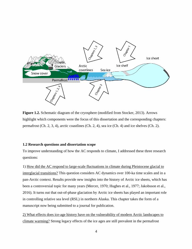
Figure 1.2. Schematic diagram of the cryosphere (modified from Stocker, 2013). Arrows
highlight which components were the focus of this dissertation and the corresponding chapters:
permafrost (Ch. 2, 3, 4), arctic coastlines (Ch. 2, 4), sea ice (Ch. 4) and ice shelves (Ch. 2).
1.2 Research questions and dissertation scope
To improve understanding of how the AC responds to climate, I addressed these three research
questions:
1) How did the AC respond to large-scale fluctuations in climate during Pleistocene glacial to
interglacial transitions? This question considers AC dynamics over 100-ka time scales and in a
pan-Arctic context. Results provide new insights into the history of Arctic ice sheets, which has
been a controversial topic for many years (Mercer, 1970; Hughes et al., 1977; Jakobsson et al.,
2016). It turns out that out-of-phase glaciation by Arctic ice sheets has played an important role
in controlling relative sea level (RSL) in northern Alaska. This chapter takes the form of a
manuscript now being submitted to a journal for publication.
2) What effects does ice-age history have on the vulnerability of modern Arctic landscapes to
climate warming? Strong legacy effects of the ice ages are still prevalent in the permafrost

5
landscapes of Arctic Alaska. Much of the permafrost in the AC formed during the Pleistocene,
and as such, depositional environments at this time exerted a lot of control over the morphology
and volume of ground ice. How permafrost landscapes will respond to future climate changes
depends primarily on ground ice volume and cryostratigraphy and the level of protection
provided by overlying organic layers. Pleistocene geologic units can inform us about the
vulnerability of a landscape to thaw. This chapter was published as an article in the journal
Geomorphology (Farquharson et al., 2016).
3) What feedbacks exist between the AC’s land and ocean components? Sea ice is declining
rapidly in the Chukchi Sea, with the duration of the sea-ice season decreasing by approximately
10% per decade. This means the coastlines of Bering Land Bridge National Park and Cape
Krusenstern National Monument are exposed to more wave energy for a longer period each year.
In this chapter, I investigate how the permafrost coasts of the southeast Chukchi Sea are
responding to warming climate and an altered sea-ice regime. This chapter has been submitted as
a report to the funding agency (US National Park Service) and will be submitted as an article in a
scientific journal.
For each component of my PhD research, I was the lead on study design, data collection, data
analysis, and manuscript writing.
1.3 References
Anderson, R.S. and Anderson, S.P., 2010. Geomorphology: the mechanics and chemistry of
landscapes. Cambridge University Press.
Barnhardt, W.A., Gehrels, W.R. and Kelley, J.T., 1995. Late Quaternary relative sea-level
change in the western Gulf of Maine: Evidence for a migrating glacial forebulge. Geology,
23(4), pp.317-320.
Cohen, J., Screen, J.A., Furtado, J.C., Barlow, M., Whittleston, D., Coumou, D., Francis, J.,
Dethloff, K., Entekhabi, D., Overland, J. and Jones, J., 2014. Recent Arctic amplification
and extreme mid-latitude weather. Nature geoscience, 7(9), pp.627-637.
6
DeJong, B.D., Bierman, P.R., Newell, W.L., Rittenour, T.M., Mahan, S.A., Balco, G. and Rood,
D.H., 2015. Pleistocene relative sea levels in the Chesapeake Bay region and their
implications for the next century. GSA Today, 25(8), pp.4-10.
Derksen, C., Brown, R., Mudryk, L. and Luojus, K., 2015. Terrestrial Snow (in “State of the
Climate in 2014”). Bull. Am. Meteorol. Soc. 96 (7), S139–S141.
Farquharson, L.M., Mann, D.H., Grosse, G., Jones, B.M. and Romanovsky, V.E., 2016. Spatial
distribution of thermokarst terrain in Arctic Alaska. Geomorphology, 273, pp.116-133.
Hughes, T., Denton, G.H. and Grosswald, M.G., 1977. Was there a late-Wiirm Arctic ice sheet.
Nature, 266(5603), p.5967602.
Jakobsson, M., Nilsson, J., Anderson, L., Backman, J., Björk, G., Cronin, T.M., Kirchner, N.,
Koshurnikov, A., Mayer, L., Noormets, R. and O'regan, M., 2016. Evidence for an ice shelf
covering the central Arctic Ocean during the penultimate glaciation. Nature
communications, 7.
Mahoney, A.R., Eicken, H., Gaylord, A.G. and Gens, R., 2014. Landfast sea ice extent in the
Chukchi and Beaufort Seas: The annual cycle and decadal variability. Cold Regions Science
and Technology, 103, pp.41-56.
Mercer, J.H., 1970. A former ice sheet in the Arctic Ocean?. Palaeogeography,
Palaeoclimatology, Palaeoecology, 8(1), pp.19-27.
Miller, G.H., Alley, R.B., Brigham-Grette, J., Fitzpatrick, J.J., Polyak, L., Serreze, M.C. and
White, J.W., 2010. Arctic amplification: can the past constrain the future?. Quaternary
Science Reviews, 29(15), pp.1779-1790.
Overland, J.E. and Wang, M., 2013. When will the summer Arctic be nearly sea ice free?.
Geophysical Research Letters, 40(10), pp.2097-2101.
Peltier, W.R., 2004. Global glacial isostasy and the surface of the ice-age Earth: the ICE-5G
(VM2) model and GRACE. Annu. Rev. Earth Planet. Sci., 32, pp.111-149.
Ritter, D.F., Kochel, R.C. and Miller, J.R., 1995. Process geomorphology. Boston: McGraw-Hill.
Romanovsky, V.E., Smith, S.L., Christiansen, H.H., 2010. Permafrost thermal state in the polar
northern hemisphere during the international polar year 2007–2009: a synthesis. Permafr.
Periglac. Process. 21, 106–116.

7
Romanovsky, V.E., Smith, S.L., Christiansen, H.H., Shiklomanov, N.I., Streletskiy, D.A.,
Drozdov, D.S., Malkova, G.V., Oberman, N.G., Kholodov, A.L., Marchenko, S.S., 2015.
Terrestrial Permafrost (in “State of the Climate in 2014”). Bull. Am. Meteorol. Soc. 96 (7),
S139–S141.
Screen, J.A. and Simmonds, I., 2010. The central role of diminishing sea ice in recent Arctic
temperature amplification. Nature, 464(7293), p.1334.
Screen, J.A., 2017. Climate science: Far-flung effects of Arctic warming. Nature Geoscience,
10(4), pp.253-254.
Serreze, M.C. and Barry, R.G., 2011. Processes and impacts of Arctic amplification: A research
synthesis. Global and Planetary Change, 77(1), pp.85-96.
Shackleton, N.J., 1987. Oxygen isotopes, ice volume and sea level. Quaternary Science Reviews,
6(3), pp.183-190.
Stocker, T.F., Qin, D., Plattner, G.K., Tignor, M., Allen, S.K., Boschung, J., Nauels, A., Xia, Y.,
Bex, B. and Midgley, B.M., 2013. IPCC, 2013: climate change 2013: the physical science
basis. Contribution of working group I to the fifth assessment report of the
intergovernmental panel on climate change.
Stroeve, J.C., Kattsov, V., Barrett, A., Serreze, M., Pavlova, T., Holland, M. and Meier, W.N.,
2012. Trends in Arctic sea ice extent from CMIP5, CMIP3 and observations. Geophysical
Research Letters, 39(16).
Tarnocai, C., Canadell, J.G., Schuur, E.A.G., Kuhry, P., Mazhitova, G. and Zimov, S., 2009. Soil
organic carbon pools in the northern circumpolar permafrost region. Global biogeochemical
cycles, 23(2).
Wendler, G., Shulski, M. and Moore, B., 2010. Changes in the climate of the Alaskan North
Slope and the ice concentration of the adjacent Beaufort Sea. Theoretical and Applied
Climatology, 99(1-2), pp.67-74.
Zimov, S.A., Schuur, E.A. and Chapin, F.S., 2006. Permafrost and the global carbon budget.
Science, 312(5780), pp.1612-1613.

8
9
Chapter 2 Marine transgressions in northern Alaska indicate out-of-phase Beaufort Sea
glaciation during the last interglacial1
2.1 Abstract
The extent and timing of ice sheets and ice shelves in the Arctic Ocean remain enigmatic despite
>50 years of scientific debate. Here we use a new suite of optically stimulated luminescence
(OSL) dates to constrain the timing of marine transgressions during MIS 5 (marine isotope stage
5) along Alaska’s Beaufort Sea coast that reflect the presence of ice shelves offshore. Deposits of
the Pelukian Transgression (PT) form a barrier-island system now 10 m above sea level, and
OSL dates show this barrier was deposited during the last four sub-stages of MIS 5 (80-113 ka).
This means the PT occurred after the warmest part of the last interglacial (129-116 ka) and was
not coeval with the eustatic maximum occurring elsewhere in the world during MIS 5e. Age and
elevational differences between stratigraphic sections suggest the Pelukian barrier system is a
composite feature built by several different marine transgressions. The most likely cause of these
transgressions was isostatic depression under the grounded margins of ice shelves in the Arctic
Ocean that existed as components of polar ice sheets located over the Canadian Arctic
Archipelago. These results confirm and provide a new chronological basis for extensive Arctic
glaciation that was out-of-phase with ice sheets at lower latitudes.
1 L.M. Farquharson, D.H. Mann, T. Rittenour, B. M. Jones, G. Grosse, P. Groves. In Preparation.
for Nature Geoscience, Marine transgressions in northern Alaska indicate out-of-phase Beaufort
Sea glaciation during the last interglacial

10
2.2 Introduction
Changes in glacier extent and relative sea level (RSL) along the Beaufort Sea coastline of Alaska
during the last interglacial (Marine Isotope Stage (MIS) 5, ~130- 80 ka) (Lisiecki and Raymo,
2005) provide insights into how the Arctic cryosphere responds to climate states different from
the present. Globally, peak warmth occurred during MIS substage 5e, ca. 129-116 ka BP (CAPE
Members, 2006; Tzedakis et al., 2012) when mean annual temperatures were 4-5°C higher than
today in the Arctic (Miller et al., 2010) and relative sea level (RSL) stood 6-9 m higher in many
parts of the world (Dutton et al., 2015). Two other warm substages (MIS 5a and 5c) occurred
later in MIS 5, ca. 113-80 ka BP, and were accompanied by eustatic sea level fluctuations of
some 40 m (Rohling et al., 2008; Spratt and Lisiecki, 2016). One of the primary drivers of
fluctuations in sea level was the build-up and decay of high-latitude glaciers. The extent and
timing of high-latitude glaciers to climatic conditions during MIS 5a and 5c are interesting
because these conditions were intermediate between full glacial and full interglacial conditions.
Raised marine deposits along Alaska’s Arctic coast provide insights into the extent of Arctic
Basin glaciation during these intermediate times.
Alaska’s Arctic Coastal Plain contains a complex archive of marine, alluvial, glacial, and aeolian
deposits spanning the Cenozoic (Dinter et al., 1990). One of the most striking paleo-shoreline
features is a barrier island system now lying 6-10 m asl and stretching 180 km from Point
Barrow eastward to the Colville River delta (Figure 2.1). The RSL rise that formed this raised
barrier system has been termed the Pelukian Transgression (PT) (Hopkins, 1967; Brigham-Grette
and Hopkins, 1995).
The altitude of PT deposits and the fact they contain extralimital, southern, marine mollusk
species initially suggested this marine transgression was caused by the RSL highstand during
MIS 5e (Kaufman and Brigham-Grette, 1993); however, until now the age of the PT has
remained uncertain. Although amino acid epimerization is useful correlating raised marine
deposits on widely separated Arctic coasts on glacial to interglacial time-scales (Kaufman and
Brigham-Grette, 1993), this method does not determine absolute age (Miller and Brigham-
Grette, 1989; Mangerud and Svendsen, 1992), and racemization rates are too slow in the Arctic
Alaska to resolve deposits separated in age by <60 ka (Brigham-Grette and Hopkins, 1995).

11
Carter et al (1986) obtained thermoluminescence dates on PT deposits near Teshekpuk Lake
ranging between 108 and 140 ka, but Brigham-Grette and Hopkins (1995) dismissed these results
as unreliable for methodological reasons and because the ages appeared to be too young to
coincide with global sea level fluctuations. Since that time, optically stimulated luminescence
(OSL) dating methods have improved greatly and our understanding of arctic basin glaciations
has progressed.
Determining the age of the PT has taken on new significance as the long-running controversy
about ice-sheet glaciation in the Arctic Basin (Mercer, 1970, Hughes et al., 1977; Broecker,
1975) heats up again (Jakobsson et al., 2016). Although the pan-Arctic ice sheets and ice shelves
envisioned by Hughes et al., (1977) were initially dismissed because of a lack of field evidence,
new geomorphological evidence supports the presence of grounded ice sheets in the Beaufort
Sea (Engels et al., 2008, Jakobsson et al., 2008), the Chukchi Sea (Polyak et al., 2001, Dove et
al., 2014, Niessen et al., 2013), and over the Lomonosov Ridge in the central Arctic Basin
(Jakobsson, et al., 2010, 2016). However, dating ancient ice-sheet glaciations in the Arctic
presents major challenges, mainly because the best field evidence is preserved on the sea bed.
Cold-based glaciers and the margins of floating ice-shelves leave only subtle geological evidence
on land and much of the onshore evidence of ancient ice sheets and ice shelves has been effaced
by later glaciation and RSL change. As a result, existing estimates for when ice sheets built up
on the shores of the Arctic Ocean rely on limiting ages based on biostratigraphic correlations in
deep-sea cores (Jakobsson et al, 2016). These age estimates suggest that at least once during MIS
6 (190-120 ka), and at possibly on several later occasions, extensive ice shelves >1 km in total
thickness existed in the Arctic Ocean (Jakobsson et al., 2016; Zhao et al., 2017). The most secure
age constraint is that one or more episodes of trans-Arctic Ocean glaciation occurred before the
last glacial maximum (LGM, ~21 ka) (Jakobsson et al., 2010, Brigham-Grette, 2013).
Raised shoreline deposits along Alaska’s Beaufort Sea coast may contain valuable information
about Arctic Ocean ice sheets and their ice shelves. The goals of this study are to use the OSL
technique to date deposits of the PT, to hypothesize about its glacio-isostatic mechanisms, and to
explore the implications of the timing of the PT for the glacial history of the Arctic.
12
2.3 Multiple marine transgressions during MIS 5
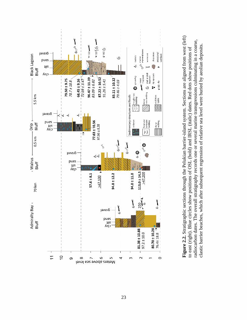
Section stratigraphy (six sites spanning 80 km) is consistent with the PT deposits representing a
landward-migrating, barrier-island system (Short 1979, Jordan and Mason, 1999, Reineck and
Singh, 2012) (Appendix A). Sediment deposited in brackish lagoons and tidal flats lies at the
base of five of the six sections (Figure 2.2). In the lower 4 m of the Black Lagoon section, lagoon
and tidal flat facies alternate, possibly recording the longshore migration of a tidal inlet and/or a
fluctuation in RSL. Occasional boulders of reddish and grey igneous rocks that occur in the
lower 1 m of the Walrus and Black Lagoon sections and are scattered along the northern shore of
Teshekpuk Lake (Appendix A) are – like the stratigraphically younger Flaxman Member of the
Gubik Formation (Rodeick, 1979) - glacial erratics derived from the Canadian Arctic
Archipelago.
At first glance, the presence of extralimital mollusk species in the PT deposits indicate climate
was warmer than today, an inference consistent with a MIS 5e age (Carter et al., 1986;
McDougall, 1994; Brigham-Grette and Hopkins 1995). On the other hand, none of the ca. 100
bivalve shells (Appendix A) we found in the sections were in growth position, so they could
have been reworked, possibly from MIS 5e deposits located seaward and at lower altitude.
Because of the possibility of reworking and the uncertainties inherent in amino-acid dating of
these shells (Brigham-Grette and Hopkins, 1995), the presence of southern, warm-water
mollusks is not a definitive criterion for assigning the PT to the warmest substage of the last
interglacial, MIS 5e.
OSL dates on the PT deposits range from 113.0 ± 14.5 to 68.45 ± 9.16 ka (Figure 2.2, Appendix
A). The post-120 ka ages (n=10) indicate that the peak of the transgression, evidenced by the
barrier beach units, occurred after the warmest part of the last interglacial (MIS 5e, 129-116 ka).
The distribution of the OSL ages suggests the Pelukian barrier system formed during two main
periods: 90-77 ka BP at the Black Lagoon section and 110 -95 ka BP at the Walrus section
(Figure 2.3). Together with the fact that similar sedimentary facies occur at different elevations
in some of the sections (Figure 2.2), this bi-modal timing suggests the Pelukian barrier system
was built by more than one marine transgression. The lagoon unit at the base of Walrus Bluff
produced the oldest age (113.0+/- 14.5), which overlaps in time with MIS 5e. A possible

13
explanation is this lagoon existed landward of a MIS 5e barrier whose crest was seaward and at
lower altitude than the Pelukian barrier system forming subsequently. Complex on- and off-
lapping relationships are expected along an ancient coastal plain bordering an ocean with a long
history of changes in both eustatic sea level and glacial extent.
What could have caused marine transgressions to reach ~10 m above present sea level sometime
after the peak in eustatic sea level during MIS 5e? Tectonism can be excluded given the long-
term stability of this trailing continental margin (Grantz et al., 1979, Shephard et al., 2013). We
suggest two alternate explanations, both involving glacio-isostasy: 1) the collapse of a glacial
forebulge generated by the Laurentide Ice Sheet (Fig 2.4a), and 2) localized isostatic depression
under the grounded margin of a floating ice shelf in the Beaufort Sea (Fig 2.4b).
Hypothesis 1. Collapse of a glacial forebulge: Loading under ice sheets can cause crustal
deformation, displacement of the underlying mantle, and subsequent uplift of a forebulge in the
surrounding unglaciated terrain (Fjeldskaar 1994; Dyke and Peltier 2000; Peltier, 2004). By
analogy with the situation along the eastern seaboard of the United States (DeJong et al., 2015),
the PT may have been caused by a forebulge generated by the Laurentide Ice Sheet (LIS) in
northwestern, mainland Canada and/or by the Innuitian Ice Sheet (IIS) in the Canadian Arctic
Archipelago, either during MIS 6 or during out-of-phase glaciation sometime in MIS 5. After the
LIS retreated at the end of MIS 6, this forebulge would have collapsed and migrated eastward,
resulting in the subsidence of the Beaufort Sea Coast and its intersection with sea level during
highstands of eustatic sea level during MIS 5a (~82 ka BP) and/or MIS 5c (~96 ka BP) (Figure
2.4a). A second forebulge generated by the LIS or IIS during the LGM was then responsible for
raising PT deposits high enough so that they remain above sea level today.
Arguing against the forebulge hypothesis is its prediction that Alaska’s Beaufort Sea coastline is
currently subsiding as the LGM forebulge dissipates eastward. In fact, the western Beaufort Sea
coast shows no geomorphological indications, such as drowned gullies and estuaries, that a
marine transgression is underway today. Instead, the geodynamics model of Peltier et al., (2015)
locates the remnant LGM forebulge over the eastern Canadian Arctic Archipelago today (Fig

14
2.1A) (Tarasov and Peltier, 2004; Snay et al., 2016), where in fact a marine transgression is now
in progress (Lajeunesse and Hansen, 2008).
Hypothesis 2. Isostatic depression under the grounded margin of an Arctic Ocean ice shelf: A
second possibility is that the PT was caused by isostatic depression under the grounded margin
of an Arctic Ocean ice shelf impinging on the Beaufort Sea coastline. Fluctuations in the
thickness and extent of this grounded ice shelf, in conjunction with fluctuating eustatic sea level
during the latter four substages of MIS 5 could have caused multiple high stands in RSL (Figure
2.4b). This hypothesis makes two predictions: 1) The Arctic experienced glacial advances during
MIS 5 that were out-of-phase with lower latitude glaciations such that isostatic depression
caused by these ice masses occurred at times of relatively high eustatic sea level. 2) Thick ice
shelves existed in the Arctic Ocean, and at times their margins were grounded along Alaska’s
Beaufort Sea coast.
Multiple lines of evidence indicate polar ice sheets were at times out-of-phase with global ice
volumes, especially during the shoulder intervals of glacial-interglacial transitions. Examples
include an ancient ice cap over Chukotka (Brigham-Grette et al., 2001), the IIS (England et al.,
2006) and northernmost sectors of the LIS (Andrews et al., 1972; Dyke and Prest, 1987) during
the LGM, portions of the Antarctic ice sheets (Denton and Hughes, 2002), glaciers in Svalbard
(Mangerud and Svensen, 1992), the Barents Sea Ice Sheet (Jakobsson et al., 2014), and Arctic
Ocean ice sheets and ice shelves (Jakobsson et al., 2016). The estimated ages of these out-of-
phase high-latitude glaciations are generally poorly constrained but often fall within MIS 5
(~130-80 ka) at a time when major changes in eustatic sea level reflecting large changes in
global ice volume occurred in the absence of extensive ice sheets at lower latitudes (Waelbroeck
et al., 2002; Zheng et al., 2002; Rohling et al., 2008; Kaplan et al., 2008).
Mounting evidence indicates the existence of thick ice shelves offshore in the Beaufort Sea on
one or more occasions in pre-LGM times (Fig 2.1A) (Jakobsson et al., 2016). Sea-floor scouring
on bathymetric high points in the Arctic Ocean demonstrates that ice shelves up to 1000 m thick
at times flowed out of the western Arctic Basin across the North Pole towards the Nordic Seas
(Polyak et al., 2001; Niessen et al., 2013; Jakobsson et al., 2016).

15
These ice sheets were fed by ice domes that were partially land-based, one of the largest located
somewhere over the Canadian Arctic Archipelago east of the Alaskan Beaufort Sea coast (Stokes
et al., 2006; Engels et al., 2008; Polyak et al., 2001; Batchelor et al., 2014). This same region is
the probable source area for the erratics boulders occurring in both the Flaxman and the PT
deposits on the Alaskan coast (Rodeick, 1979). Buried glacial ice of pre-LGM age that was
possibly left by the grounded margin of an Arctic Ocean ice shelf occurs at several locations
along the Beaufort Sea coast beyond the maximum extent of the LIS during the LGM
(Kanevskiy et al., 2013). Also along the Beaufort Sea coast, large-scale lineations and scours up
to 700 m below modern sea level are consistent with the presence of a thick, westward-flowing
ice shelf whose margin was grounded along the Alaskan coast (Figure 2.1A) (Engels et al.,
2008). Isostatic depression under a grounded ice shelf could have caused the PT (-s).
2.4 Terrestrial-based evidence for an out-of-phase grounded ice shelf in the Arctic Ocean
during MIS 5
New OSL ages indicate the PT (-s) occurred during the later substages of the last interglacial
subsequent to MIS 5e and that it was out-of-phase with the global MIS 5e high stand in eustatic
sea level and the global minimum in ice volume reflected by that RSL high stand. Altitudinal
differences between barrier-beach units in different stratigraphic sections suggest the PT
consisted of more than one RSL rise. The most probable cause of the PT was isostatic depression
under the grounded margin of an ice shelf that was fed by a polar ice sheet centered over the
Canadian Arctic Archipelago. For barrier island formation to take place there must have been
some distance between the ice shelf edge and the coastline. The age of the PT indicates
glaciation in this sector of the Arctic Basin was out-of-phase with ice-sheet glaciation at lower
latitudes.

16
Acknowledgements
LMF was funded by the UAF Center for Global Change. We thank M. Nelson at the USU OSL
Laboratory for running OSL samples, Nora Foster at NRS Taxonomic Services for gastropod
identification, Dyke Scheidemann at AWI for assistance with grain size analysis, and both the
Teshekpuk Lake Observatory and North Slope Borough for providing shelter while conducting
field work. Any use of trade, product, or firm names is for descriptive purposes only and does
not imply endorsement by the US Government.
2.5 References
Andrews, J.T., Mears, A., Miller, G.H. and Pheasant, D.R., 1972. Holocene late glacial
maximum and marine transgression in the eastern Canadian Arctic. Nature, 239(96),
pp.147-149.
Batchelor, C.L., Dowdeswell, J.A. and Pietras, J.T., 2014, Evidence for multiple Quaternary ice
advances and fan development from the Amundsen Gulf cross-shelf trough and slope,
Canadian Beaufort Sea margin: Marine and Petroleum Geology, 52, pp.125-143.
Brigham-Grette, J. and Hopkins, D.M., 1995, Emergent marine record and paleoclimate of the
last interglaciation along the northwest Alaskan coast: Quaternary Research, 43(2), pp.159-
173.
Brigham-Grette, J., Hopkins, D.M., Ivanov, V.F., Basilyan, A.E., Benson, S.L., Heiser, P.A. and
Pushkar, V.S., 2001. Last Interglacial (isotope stage 5) glacial and sea-level history of
coastal Chukotka Peninsula and St. Lawrence Island, Western Beringia. Quaternary Science
Reviews, 20(1), pp.419-436.
Brigham-Grette, J., 2013, A fresh look at Arctic ice sheets: Nature Geoscience, 6, 807-808
Broecker, W.S., 1975, Climatic change: are we on the brink of a pronounced global warming?:
Science, pp.460-463.
Bronk Ramsey, C., 2013, OxCal 4.2: Web Interface Build (78).
CAPE-Last Interglacial Project, 2006, Last Interglacial Arctic warmth confirms polar
amplification of climate change: Quaternary Science Reviews, 25 (13), pp. 1383-1400.

17
Carter, L.D., Brigham-Grette, J. and Hopkins, D.M., 1986, Late Cenozoic marine transgressions
of the Alaskan Arctic coastal plain. In Correlation of Quaternary deposits and events around
the margin of the Beaufort Sea: contributions from a joint Canadian-American workshop,
pp. 21-26.
Carter, L.D., and Robinson, S.W., 1981, Minimum age of beach deposits north of Teshekpuk
Lake, Alaskan Arctic Coastal Plain, in Albert, N.R.D., and Hudson, Travis, eds., The United
States Geological Survey in Alaska; accomplishments during 1979: U.S. Geological Survey
Circular 823-B, p. B8-B9.
DeJong, B.D., Bierman, P.R., Newell, W.L., Rittenour, T.M., Mahan, S.A., Balco, G. and Rood,
D.H., 2015, Pleistocene relative sea levels in the Chesapeake Bay region and their
implications for the next century: GSA Today, 25(8), pp.4-10.
Denton, G.H. and Hughes, T.J., 2002. Reconstructing the Antarctic ice sheet at the Last Glacial
Maximum. Quaternary Science Reviews, 21(1), pp.193-202.
Dinter, D., Carter, L.D. and Brigham-Grette, J. (1990). Late Cenozoic geologic evolution of the
Alaskan North Slope and adjacent continental shelves. In: Grantz, J., Johnson, L. and
Sweeney, J.F. (eds), The Geology of North America, V.L., The Arctic Region, pp. 459
Dove, D., Polyak, L. and Coakley, B., 2014, Widespread, multi-source glacial erosion on the
Chukchi margin, Arctic Ocean: Quaternary Science Reviews, 92, pp.112-122.
Dutton, A., Carlson, A.E., Long, A.J., Milne, G.A., Clark, P.U., DeConto, R., Horton, B.P.,
Rahmstorf, S. and Raymo, M.E., 2015, Sea-level rise due to polar ice-sheet mass loss
during past warm periods: Science, 349 (6244)
Dyke, A. and Prest, V., 1987. Late Wisconsinan and Holocene history of the Laurentide ice
sheet. Géographie physique et Quaternaire, 41(2), pp.237-263.
Dyke, A.S. and Peltier, W.R., 2000, Forms, response times and variability of relative sea-level
curves, glaciated North America: Geomorphology, 32(3), pp.315-333.
Engels, J.L., Edwards, M.H., Polyak, L. and Johnson, P.D., 2008, Seafloor evidence for ice shelf
flow across the Alaska–Beaufort margin of the Arctic Ocean: Earth Surface Processes and
Landforms, 33(7), pp.1047-1063.
England, J., Atkinson, N., Bednarski, J., Dyke, A.S., Hodgson, D.A. and Cofaigh, C.Ó., 2006,
The Innuitian Ice Sheet: configuration, dynamics and chronology. Quaternary Science
Reviews, 25(7), pp.689-703.

18
Fjeldskaar, W., 1994, Viscosity and thickness of the asthenosphere detected from the
Fennoscandian uplift: Earth and Planetary Science Letters, 126(4), pp.399-410.
Grantz, A., Eittreim, S. and Dinter, D.A., 1979, Geology and tectonic development of the
continental margin north of Alaska: Tectonophysics, 59(1-4), pp.263-291.
Hopkins, D.M., 1967, The Cenozoic history of Beringia—a synthesis. In: Hopkins, D.M., (Ed)
The Bering land bridge (Vol. 3). Stanford University Press.
Hughes, T., Denton, G.H. and Grosswald, M.G., 1977, Was there a late-Wiirm Arctic ice sheet:
Nature, 266(5603), p.5967602
Jakobsson, M., Polyak, L., Edwards, M., Kleman, J. and Coakley, B., 2008, Glacial
geomorphology of the central Arctic Ocean: the Chukchi Borderland and the Lomonosov
Ridge. Earth Surface Processes and Landforms, 33(4), pp.526-545.
Jakobsson, M., Nilsson, J., O’Regan, M., Backman, J., Löwemark, L., Dowdeswell, J.A., Mayer,
L., Polyak, L., Colleoni, F., Anderson, L.G. and Björk, G., 2010, An Arctic Ocean ice shelf
during MIS 6 constrained by new geophysical and geological data: Quaternary Science
Reviews, 29(25), pp.3505-3517
Jakobsson, M., Andreassen, K., Bjarnadóttir, L.R., Dove, D., Dowdeswell, J.A., England, J.H.,
Funder, S., Hogan, K., Ingólfsson, Ó., Jennings, A. and Larsen, N.K., 2014. Arctic Ocean
glacial history. Quaternary Science Reviews, 92, pp.40-67.
Jakobsson, M., Nilsson, J., Anderson, L., Backman, J., Björk, G., Cronin, T.M., Kirchner, N.,
Koshurnikov, A., Mayer, L., Noormets, R. and O'regan, M., 2016, Evidence for an ice shelf
covering the central Arctic Ocean during the penultimate glaciation: Nature
communications, 7.
Jordan, J.W., Mason, O.K., 1999, A 5000 year record of intertidal peat stratigraphy and sea level
change from northwest Alaska: Quaternary International, 60(1), pp.37-47.
Kanevskiy, M., Shur, Y., Jorgenson, M.T., Ping, C.L., Michaelson, G.J., Fortier, D., Stephani,
E., Dillon, M. and Tumskoy, V., 2013, Ground ice in the upper permafrost of the Beaufort
Sea coast of Alaska: Cold Regions Science and Technology, 85, pp.56-70.
Kaplan, M.R., Moreno, P.I. and Rojas, M., 2008, Glacial dynamics in southernmost South
America during Marine Isotope Stage 5e to the Younger Dryas chron: a brief review with a
focus on cosmogenic nuclide measurements: Journal of Quaternary Science, 23(6‐7),
pp.649-658.

19
Kaufman, D.S. and Brigham-Grette, J., 1993, Aminostratigraphic correlations and
paleotemperature implications, Pliocene-Pleistocene high-sea-level deposits, northwestern
Alaska: Quaternary Science Reviews, 12(1), pp.21-33.
Lajeunesse, P. and Hanson, M.A., 2008, Field observations of recent transgression on northern
and eastern Melville Island, western Canadian Arctic Archipelago: Geomorphology, 101(4),
pp.618-630.
Lisiecki, L.E. and Raymo, M.E., 2005. A Pliocene-Pleistocene stack of 57 globally distributed
benthic δ18O records. Paleoceanography, 20(1).
Mangerud, J. and Svendsen, J.I., 1992, The last interglacial-glacial period on Spitsbergen,
Svalbard: Quaternary Science Reviews, 11(6), pp.633-664.
McDougall, K., 1994, Late Cenozoic benthic foraminifers of the HLA borehole series, Beaufort
Sea shelf, Alaska. US Government Printing Office.
Mercer, J.H., 1970, A former ice sheet in the Arctic Ocean?: Palaeogeography,
Palaeoclimatology, Palaeoecology, 8(1), pp.19-27.
Miller, G.H. and Brigham-Grette, J., 1989, Amino acid geochronology: resolution and precision
in carbonate fossils: Quaternary International, 1, pp.111-128.
Miller, G.H., Alley, R.B., Brigham-Grette, J., Fitzpatrick, J.J., Polyak, L., Serreze, M.C. and
White, J.W., 2010, Arctic amplification: can the past constrain the future?: Quaternary
Science Reviews, 29(15), pp.1779-1790.
Niessen, F., Hong, J.K., Hegewald, A., Matthiessen, J., Stein, R., Kim, H., Kim, S., Jensen, L.,
Jokat, W., Nam, S.I. and Kang, S.H., 2013, Repeated Pleistocene glaciation of the East
Siberian continental margin: Nature Geoscience, 6(10), p.842.
Peltier, W.R., 2004, Global glacial isostasy and the surface of the ice-age Earth: the ICE-5G
(VM2) model and GRACE: Annu. Rev. Earth Planet. Sci., 32, pp.111-149.
Peltier, W.R., Argus, D.F. and Drummond, R., 2015, Space geodesy constrains ice age terminal
deglaciation: The global ICE‐6G_C (VM5a) model. Journal of Geophysical Research: Solid
Earth, 120(1), pp.450-487.
Polyak, L., Edwards, M.H., Coakley, B.J. and Jakobsson, M., 2001, Ice shelves in the
Pleistocene Arctic Ocean inferred from glaciogenic deep-sea bedforms: Nature, 410(6827),
p.453.
Ramsey, C.B., 2009, Bayesian analysis of radiocarbon dates. Radiocarbon, 51(1), pp.337-360.
20
Reineck, H.E. and Singh, I.B., 2012, Depositional sedimentary environments: with reference to
terrigenous clastics. Springer Science and Business Media. New York.
Rhodes, E.J., Ramsey, C.B., Outram, Z., Batt, C., Willis, L., Dockrill, S. and Bond, J., 2003,
Bayesian methods applied to the interpretation of multiple OSL dates: high precision
sediment ages from Old Scatness Broch excavations, Shetland Isles. Quaternary Science
Reviews, 22(10), pp.1231-1244.
Rodeick, C.A., 1979, The origin, distribution, and depositional history of gravel deposits on the
Beaufort Sea continental shelf, Alaska (No. 79-234). US Geological Survey.
Rohling, E.J., Grant, K., Hemleben, C.H., Siddall, M., Hoogakker, B.A.A., Bolshaw, M. and
Kucera, M., 2008, High rates of sea-level rise during the last interglacial period: Nature
Geoscience, 1(1), pp.38-42.
Scott, T.W., Swift, D.J., Whittecar, G.R. and Brook, G.A., 2010, Glacioisostatic influences on
Virginia's late Pleistocene coastal plain deposits. Geomorphology, 116(1), pp.175-188.
Shephard, G.E., Müller, R.D. and Seton, M., 2013, The tectonic evolution of the Arctic since
Pangea breakup: Integrating constraints from surface geology and geophysics with mantle
structure: Earth-Science Reviews, 124, pp.148-183.
Short, A.D., 1979, Barrier island development along the Alaskan-Yukon coastal plains:
Geological Society of America Bulletin, 90(1 Part II), pp.77-103.
Snay, R.A., Freymueller, J.T., Craymer, M.R., Pearson, C.F. and Saleh, J., 2016, Modeling 3‐D
crustal velocities in the United States and Canada: Journal of Geophysical Research: Solid
Earth, 121(7), pp.5365-5388.
Spratt, R.M. and Lisiecki, L.E., 2016, A Late Pleistocene sea level stack: Climate of the Past,
12(4), p.1079.
Stokes, C.R., Clark, C.D. and Winsborrow, M.C.M., 2006, Subglacial bedform evidence for a
major palaeo‐ice stream and its retreat phases in Amundsen Gulf, Canadian Arctic
Archipelago: Journal of Quaternary Science, 21(4), pp.399-412.
Tarasov, L. and Peltier, W.R., 2004, A geophysically constrained large ensemble analysis of the
deglacial history of the North American ice-sheet complex: Quaternary Science Reviews,
23(3), pp.359-388.
Tzedakis, P.C., Channell, J.E., Hodell, D.A., Kleiven, H.F. and Skinner, L.C., 2012. Determining
the natural length of the current interglacial, Nature Geoscience: 5(2), p.138.

21
Waelbroeck, C., Labeyrie, L., Michel, E., Duplessy, J.C., McManus, J.F., Lambeck, K., Balbon,
E. and Labracherie, M., 2002, Sea-level and deep water temperature changes derived from
benthic foraminifera isotopic records. Quaternary Science Reviews, 21(1), pp.295-305.
Zhao, F., Minshull, T.A., Crocker, A.J., Dowdeswell, J.A., Wu, S. and Soryal, S.M., 2017,
Pleistocene iceberg dynamics on the west Svalbard margin: Evidence from bathymetric and
sub-bottom profiler data: Quaternary Science Reviews, 161, pp.30-44.s
Zheng, B., Xu, Q. and Shen, Y., 2002, The relationship between climate change and Quaternary
glacial cycles on the Qinghai–Tibetan Plateau: review and speculation: Quaternary
international, 97, pp.93-101.

22
Figures
Figure 2.1. Maps of the study area. Maps of the study area. Panel A: Green polygon is the region
of ongoing forebulge collapse following deglaciation after ca. 20 ka (Lajeunesse and Hanson,
2008; Snay et al., 2016). Blue dotted line shows maximum extent of the Laurentide Ice Sheet
(LIS) during the Last Glacial Maximum (LGM) ca. 21 ka (Dyke et al., 2000). Dotted region
shows the extent of Arctic Ocean ice shelves postulated by Jakobsson et al. (2016) during Marine
Isotope Stage 6. The Chukchi Borderlands are a region of relatively shallow sea floor containing
glacial scours (yellow lines) from ice shelves fed by ice streams issuing from the Canadian
Arctic Archipelago (Polyak et al., 2001). Other glacial scours occur in 700-m deep water along
the continental shelf break in the Beaufort Sea (Engels et al., 2008). The purple ‘x’ marks the
location of buried glacial ice located beyond the LIS’ maximum extent (Kanevskiy et al., 2013).
Red arrows are generalized flow lines for glacial ice feeding ice shelves in the Arctic Ocean that
converge over the North Pole to calve eventually into the Greenland Sea (Jakobsson et al., 2016).
The grey polygon which covers the Beaufort Sea Coast indicates the region where ice-rafted
boulders, transported from the Canadian Archipelago, have been located (Rodeick, 1979). Panel
B: Digital elevation model of the study area. The westernmost white dot is Admiralty Bay (AB),
and the two eastern dots are at Teshekpuk Lake (T1 and T2). Grey polygons show the probable
location of the ancient Pelukian barrier system (after Carter and Robinson, 1980), and dotted
lines show the southern shore of its contemporaneous lagoon.
23
Fig
ure
2.2
. S
trat
igra
phic
sec
tions
thro
ugh t
he
Pel
ukia
n b
arri
er-i
slan
d s
yst
em.
Sec
tions
are
alig
ned
fro
m w
est
(lef
t)
to e
ast
(rig
ht)
. B
lue
circ
les
show
posi
tions
of
OS
L (
bold
) an
d I
RS
L (
ital
ic)
dat
es. R
ed d
ots
show
posi
tions
of
rad
ioca
rbon d
ates
. T
he
over
all
stra
tigra
phy r
ecord
s one
or
sever
al m
arin
e tr
ansg
ress
ions
culm
inat
ing i
n a
coar
se,
clas
tic
bar
rier
bea
ches
, w
hic
h a
fter
subse
quen
t re
gre
ssio
n o
f re
lati
ve
sea
level
wer
e buri
ed b
y a
eoli
an d
eposi
ts.

24
Fig
ure
2.3
. B
ayes
ian m
odel
of
OS
L a
ges
(R
hodes
et
al.,2003;
Ram
sey
2009
) fr
om
Wal
rus
and
Bla
ck L
agoon B
luff
s. L
ight
gre
y c
urv
es s
how
init
ial
ages
wit
h t
hei
r st
andar
d e
rrors
. D
ark
gre
y
curv
es s
how
model
led a
ges
aft
er s
trat
igra
phic
posi
tion i
s ac
counte
d f
or.
The
gre
en s
had
ing
del
inea
tes
MIS
5, an
d t
he
red s
had
ing t
he
war
mes
t par
t of
the
last
inte
rgla
cial
, M
IS 5
e. A
ges
are
in
cale
ndar
yea
rs b
efore
pre
sent.
25
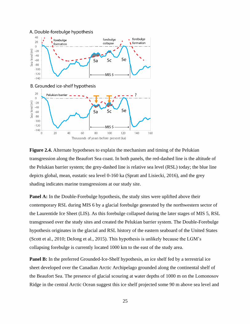
Figure 2.4. Alternate hypotheses to explain the mechanism and timing of the Pelukian
transgression along the Beaufort Sea coast. In both panels, the red-dashed line is the altitude of
the Pelukian barrier system; the grey-dashed line is relative sea level (RSL) today; the blue line
depicts global, mean, eustatic sea level 0-160 ka (Spratt and Lisiecki, 2016), and the grey
shading indicates marine transgressions at our study site.
Panel A: In the Double-Forebulge hypothesis, the study sites were uplifted above their
contemporary RSL during MIS 6 by a glacial forebulge generated by the northwestern sector of
the Laurentide Ice Sheet (LIS). As this forebulge collapsed during the later stages of MIS 5, RSL
transgressed over the study sites and created the Pelukian barrier system. The Double-Forebulge
hypothesis originates in the glacial and RSL history of the eastern seaboard of the United States
(Scott et al., 2010; DeJong et al., 2015). This hypothesis is unlikely because the LGM’s
collapsing forebulge is currently located 1000 km to the east of the study area.
Panel B: In the preferred Grounded-Ice-Shelf hypothesis, an ice shelf fed by a terrestrial ice
sheet developed over the Canadian Arctic Archipelago grounded along the continental shelf of
the Beaufort Sea. The presence of glacial scouring at water depths of 1000 m on the Lomonosov
Ridge in the central Arctic Ocean suggest this ice shelf projected some 90 m above sea level and

26
thus been capable of causing roughly 30 m of isostatic depression where it was grounded along
the Alaskan coast. This isostatic depression (vertical orange arrows) caused the Pelukian
transgression. Fluctuations in ice-shelf extent and thickness may have caused multiple
transgressions. As the ice sheet over the Canadian Arctic retreated and its associated ice shelf
disappeared, the study region rebounded causing emergence above sea level before 57+/-10ka.

27
Appendix A
Methodology, site descriptions, and chronological data for Chapter 2
Using the modern-day coasts of the Beaufort and Chukchi to aid section interpretation
To help interpret depositional environments, we examined depositional environments and
sedimentary facies along coarse clastic barrier beaches and lagoonal barrier systems along the
southern Chukchi Sea coast, a coastline characterized by less sea ice and warmer permafrost
temperatures, potentially providing an analogue for the Beaufort Sea coast during the last
interglacial.
Grain size analysis
Samples were prepared for grain size analysis by removal of organic matter in hydrogen
peroxide (H2O2, 30%). Grain size distribution was measured with a laser particle size analyser
(Coulter LS 200, Krefeld, Germany). Particles <1mm were analyzed in water, while particles
>1mm were dry-sieved through a 2mm mesh screen. We used GRADISTAT v8 (Blott and Pye
2001) for statistical analysis of grain size data.
OSL dating methodology
We used the recommendations of Bateman and Murton (2006); Murton et al., (2007), Forman et
al., (2007) to tailor or OSL sampling to the polar environment. We used optically stimulated
luminesce (OSL) quartz grains to date sections exposing sediment associated with the PT and
infra-red stimulated luminescence (IRSL) dating as a check. Prior to sampling in the field,
sections of the bluff face were broadly exposed using hand tools and the stratigraphy was
described. OSL samples were not taken near unit boundaries or lithological unconformities. We
took samples by pushing 20-cm lengths of 4-cm (inner) diameter, metal conduit pipe into freshly
cleaned exposure faces. Tube ends were capped with foam and sealed with duct tape. Sediment
for dose-rate measurements was excavated by taking a sphere of sediment from within 20 cm of
all sides of the dating sample. A small amount of material was then sealed in an air-tight

28
container for later water-content measurement. Samples were stored in cool, dark conditions and
shipped to the Utah State University OSL laboratory for analysis on return from the field.
OSL samples were opened and processed under dim amber safelight conditions in the Utah State
University OSL laboratory. Dose-rate samples were dried, homogenized and sub-sampled using
a sample splitter before being sent for geochemical analysis. Sample processing followed
standard procedures involving sieving, gravity separation, and acid treatments with HCl and HF
to isolate the quartz component of a specified grain-size range. Potassium feldspar was separated
for IRSL dating using 2.58 g/cm3 density separation with no HF pre-treatment.
Radiocarbon dating sampling method:
We used radiocarbon dating to ensure that material dated to mid- to late-Pleistocene by OSL
was of non-finite (>40,000 cal yr BP) age. Herbaceous fragments and driftwood were sampled
from coastal units at Walrus for radiocarbon dating. Samples were rinsed with distilled water and
stored in Ziplock® bags until their shipment to Beta Analytic for analysis.
Previous Pelukian chronologies:
The age of the Pelukian transgression remains uncertain in northern Alaska (Brigham-Grette and
Hopkins, 1995) and Chukotka (Brigham-Grette and Hopkins 1995). Hopkins (1967) reported
non-finite 14C ages for shells from the Pelukian type section near Nome along with a 226Ra/238U
age on shell of 78,000 years. Brigham-Grette and Hopkins (1995) compiled eleven 14C dates on
shell and wood from Pelukian deposits; nine of these ages were non-finite. Thermoluminescence
dates on shells from Pelukian deposits on the Beaufort Sea coast obtained by (Carter et al., 1986)
ranged between 108 and 140 ka but were dismissed as inaccurate by Brigham-Grette and
Hopkins (1995). While the amino acid racemization technique has proved useful in relative age
dating and correlation of raised marine deposits located on widely separated Arctic coasts
(Kaufman and Brigham-Grette, 1993), it does not furnish estimates of absolute age (Miller and
Brigham-Grette, 1989; Mangerud and Svendsen, 1992). Furthermore, because of the slow rates
of racemization in the Arctic, amino acid dating is unable to distinguish the substages of MIS 5

29
(Brigham-Grette and Hopkins 1995). Because of these issues, the Pelukian has been broadly
correlated with the eustatic sea level high-stand of MIS 5e, which Brigham-Grette and Hopkins
(1995) determine as 120-130 ka.
Out of phase glaciations in the Arctic
Increased aridity is consistently cited as a likely cause of out of phase glaciation because during
glacial periods perennial sea ice cover shuts off the Arctic Ocean as a moisture source (Ewing
and Donn, 1956; Mercer, 1970; Broecker, 1975; Dyke and Priest, 1987, de Vernal et al., 1991,
Ward et al., 2007, Brigham-Grette, 2013). As the climate transitions from glacial to interglacial
conditions, sea ice declines, and a greater area of high-latitude ocean is available as a moisture
source (de Vernal et al., 1991).
Walrus bluff section description
The Walrus section begins at lake level, which lies approximately 1 m above present sea level
(asl) (Figures A-1 and A-2, Table A-1).
Unit 1 100 – 175 cm (all elevations are given in centimeters above sea level): back-barrier
lagoon. The lowest unit (Unit 1) consists of salty, anoxic, massive, dark-grey clayey silt
containing occasional dolomite drop stones up to 10 cm in diameter (Figure A-3). We suggest
that these drop stones are of the same genesis as the Flaxman boulders (Dinter 1985) which are
thought to originate in the Amundsen Gulf (Rodeick, 1979). At the top of this unit, we found a
tibia of a ringed seal (Pusa hispida) (Figure A-4 ) and a humerus fragment from either a ribbon
or spotted seal (Phoco largha or Histriophoca fasciata). Conifer driftwood up to a 1 meter in
length is also present and one piece of this driftwood yielded a 14C age of >47.2 ka BP (Figure
A-1). We interpreted this unit to have formed within a low energy, anoxic environment, probably
a lagoon. The upper boundary transitions gradually over approximately 30 cm as flaser beds
become more frequent. We found no shells within this section.

30
Unit 2: back barrier tidal flats, 175 – 300 cm This unit consists of 125 cm of medium sand
containing cosets of flaser beds composed of sandy clay with abundant gastropod shell
fragments, none of which were in growth position. Wood fragments were commonly observed in
association with the flaser beds. The upper boundary of Unit 2 transitions comformably into Unit
3. Two OSL samples from the base and top of Unit 2 date to 113 ±15 ka (USU-1708) and 94 ±
11 ka (USU-1709), respectively (Figure A-5, Tables A-2 and A-3). We interpret this unit to be a
tidally influenced environment, possibly a back-barrier area of tidal flats where overwash events
carry in detrital wood, shell, and bone material. No drop stones were observed in this unit.
Unit 3: barrier beach, 300 - 600 cm Unit 3 consists of planar cross-beds of well-sorted medium
sand containing abundant bivalve and mollusk shells, and thin beds of coarse sand and gravel.
Bivalve and gastropod shells found include the extra-limital species Neptunea ventricosa and
Boreoscala greenlandica (Table A-4) but were not in growth position. Today the northern range
limit of these two species is the north Pacific, so their presence requires sea surface temperatures
warmer than today. The unit coarsens upwards into a massive bed of sandy gravel, lacking shells
but containing a single walrus (Odobenus rosmarus) tooth. A small sand wedge penetrates
through this layer, and is filled with well-sorted medium sand. The upper boundary of Unit 3 is
an abrupt erosional unconformity. An OSL sample from the upper meter of Unit 3 yields and age
of 94.8 ±12 ka (Figure A-5, Tables A-2 and A-3). We interpret this unit to be a barrier beach.
Unit 4: loess, 600 – 800 cm Unit 4 consists of massive, ice-rich, grey, sandy silt. An OSL age
from 700cm yielded an age of 58 ±8 (Figure A-5, Tables A-2 and A-3). A highly cryoturbated,
peaty paleosol, 70 cm thick, is located at the base of the unit and a 3 cm thick ice vein runs
through it horizontally but does not appear to penetrate the underlying unit. Herbaceous
fragments from the paleosol yielded a non-finite 14C age (>47.1 ka BP).
Drip Bluff section description
Drip Bluff section is located 500m east of Walrus and begins ~ 700 cm above sea level (Figure
A-1). Unit 1 of Drip Bluff may be contemporaneous with Walrus’s Unit 3, barrier beach
deposits.

31
Unit1, gravelly beach, 700 - 780 cm The lower 80 cm of Drip Bluff is composed of planer beds
dominated by coarse sand but also containing gravel (mean grain size for the unit is 0.7 mm) and
has an abrupt upper boundary which lies in contact with Unit 2. An OSL sample from 30 cm
below the upper boundary of this unit yielded and age of 78 +/- 11 ka (USU-2101, Figure A-5,
Tables A-2 and A-3).
Unit 2, ice-rich silty sand sheet, 780 – 850 cm Unit 2 is composed of 70 cm of poorly sorted silty
sandy organic- and ice-rich goo with rootlets, black organic inclusions and occasional pebbles.
Mean grain size is 57 µm, very fine sandy silt. The unit is capped by 30 cm of multiple moss-
peat bands interbedded with root rich pebbly silt, capped by a distinct 2cm band of coarse sand.
We suggest that Unit 2 within Drip Bluff, may be the same as Unit 4 at Walrus Bluff.
Unit 3, sand sheet, 850 – 1030 cm Unit 3 is composed of 180 cm of sand sheet deposits
composed of silty fine sand containing abundant fine rootlets. The upper 280 cm to the bluff top
and modern-day surface was not studied in detail but is composed of highly distorted organic and
ice-rich loess deposits containing syngenetic ice wedges. No grain size analysis was conducted
on this unit.
We interpret Drip Bluff to show gravelly beach deposits from MIS 3 which are overlain
unconformably by Unit 2, an ice-rich silty sand sheet containing multiple paleosols.
Black Lagoon Bluff section description
Black Lagoon Bluff section is located ca. 6 km east of Walrus (Table A-1) and begins 3.5 m
above sea-level and stretches approximately 10 meters along the shore (Figure A-2).
Unit 1, anoxic lagoon, 350 – 530cm This unit consists of salty anoxic clayey silt and contains
rare detrital shell fragments which were not in growth position. Alternating planar beds of
organic rich clay sand silt occur throughout the unit. Grain size distribution is unimodal and the
sediment is poorly sorted medium silt to very fine sand. The mean grain size ranges from 7.0 to
76 µm (n=3). The transition into Unit 2 occurs over a gradual comformable boundary spanning
60 cm and is OSL dated to 83 +/-10 (USU-2093, Figure A-5, Tables A-2 and A-3).

32
We interpret this unit to be a low energy anoxic environment, likely a lagoon. Poor sediment
sorting may be due to ice rafted debris during breakup (Barnes et al., 1982), or barrier over-wash
events during storms (Reimnitz and Barnes, 1987).
Unit 2, tidal flat, 530 – 590 cm This unit consists of multiple composite cosets of flaser cross-
laminations in muddy sand, recording flow towards 180°. The upper 10 cm of this unit contains
scattered Naticidae (Table A-4). Grain size distribution is unimodal, well sorted silty sand, and
has a mean grain size of 76.6 µm. The transition from Unit 2 to Unit 3 is a planar erosional
unconformity.
Unit 3, tidal flat, 590 – 670 cm The lower 15 cm consist of planar cross beds of medium sand,
with flow towards 130°. Worm tubes of varying morphology are common, along with a
scattering of bivalves possibly in growth position. Sediment compaction prevented us from
sampling identifiable fragments of bivalve shells for analysis. The upper 60 cm of Unit 3 consist
primarily of upward coarsening medium sand characterized by trough cross beds and oscillation
ripples. Grain size distribution is unimodal and poorly sorted. Mean grain size is 72 µm, very
fine sand. An OSL sample from this unit yielded and age of 87 +/- 11 (USU-2094, Figure A-5,
Tables A-2 and A-3). The upper boundary of Unit 3 transitions comformably into Unit 4.
Unit 4, tidal flat, 670 – 745 cm Unit 4 is composed of gravelly fine sand and contains flaser and
oscillation ripples. The upper surface is conformable with the overlaying mud, Unit 5. Two small
channels 30 cm deep and 80 cm wide, oriented to 130°, have incised into the top of Unit 4 and
are infilled with gravelly muddy sand. We interpret these channels to be part of a dendritic
channel network associated with tidal flow. Within this unit, grain size is unimodal and the
sediment moderately sorted. Mean grain size is 121 µm, fine sand. An OSL sample from the
upper 20 cm of Unit 4 yielded and age of 96+/-22 (USU-2097, Figure A-5, Tables A-2 and A-3).
Unit 5, anoxic lagoon or thaw pond close to shore, 745 – 785 cm Unit 5 is composed of dark
grey anoxic sandy silt. The upper boundary of Unit 5 is an erosional unconformity. Grain size
distribution is unimodal and the sediment very poorly sorted. Mean grain size is 43 µm. Unlike
the lower clayey silt unit, we found no shell fragments and the sediment was not salty to taste.

33
Wood fragments were frequently present. The sediment was crudely stratified and contained
occasional pebbles and sand lenses. An OSL sample from this unit yielded and age of 68 +/-9
(USU-2096, Figure A-5, Tables A-2 and A-3). The middle of the unit has formed into a large
diapir extending upwards and intruding into Unit 6.
Unit 6, pebbly beach, 785 – 1085 cm The base of unit six is composed of well sorted medium
sand with a mean grain size of 282 µm, which coarsens upward. Throughout the unit as planar
beds of pebbly sand with large lenses of poorly sorted coarse sand, and fine to coarse gravel. The
upper meter of this section is obscured by slumping. An OSL sample from the lower 20 cm of
this unit yielded an age of 80 +/- 10 years (USU-2097, Figure A-5, Tables A-2 and A-3).
Fox Cub Bluff section description
Fox Cub Buff is located approximately 330 m east of Black Lagoon Bluff (Table A-1). Grain
size analysis was conducted at 10 points up through the section (Figure A-6), and reveals an
upward coarsening sequence.
Unit 1, anoxic lagoon, 100-150 cm Unit 1 consists of 50 cm of solid grey, poorly sorted, slightly
gravelly mud which transitions conformably into the overlying unit. Mean grain size ranges from
5.3 – 6.0 µm (n=3) (Table A-6).
Unit 2, tidal flats, 150 – 250 cm Unit 2 consists of 100 cm of muddy sand characterized by
lenticular and wavy bedding. Grain size distribution in the lower 50 cm of the unit is bimodal,
and the upper 50 cm moderately to poorly sorted and unimodal. The section is composed of 50
cm of solid grey organic rich clay which transitions comfortably into 100 cm of sandy, muddy,
lenticular and wavy bedding. We interpret this unit to represent a transition from anoxic lagoonal
conditions into silty tidal flats.
We interpret Fox Bluff to show a shallow tidally influenced coastal area. Upwards coarsening
suggesting a transition from a deeper to shallower environment, perhaps due to the migration of a
barrier island, tidal channel or tidal delta. The presence of gravel may be due to ice rafted debris.
Each unit was analyzed for diatoms but none were found.

34
Lost Log Bluff description
The Lost Log section is located approximately 6 km east of Walrus, close to Black Lagoon Bluff
(Table A-1).
Unit 1, anoxic lagoon, 100-150 cm Unit 1 is composed of dark grey salty poorly sorted fine silt
containing no shells. The erosional upper boundary shows signs that blocks of sediment have
been eroded away (rip up clasts) possibly due to freezing and plucking.
Unit 2, tidal flats, 150 – 175 cm Unit 2 is a 25 cm thick trash layer containing planar beds of
medium sand and black silty clay, interspersed with abundant wood and shell fragments, not in
growth position. The black silty clay appears to be the same as the clay present in Unit 1 of this
section. Small inclusions of coarse sand and pebbles occur throughout the unit.
Unit 3, barrier beach, 175 – 220 cm Unit 3 is composed of 45 cm of pebbly granules in a medium
to coarse sand matrix with abundant shell fragments. This unit dips towards 170° and contains
rip up clasts, probably from lowest section.
Unit 4, barrier beach, 220 -290 cm Unit 4 is composed of 70 cm of medium fine sand, in co-sets
of fluvial planar cross beds. A band of rip up clasts and clay approximately 4 cm thick, runs
through the center of the unit. Above this band is 30 cm of planar cross beds composed of shell-
fragment rich medium to fine sand. Beds within this unit dip towards 180°.
Unit 5, aeolian dune, 290 -340 cm Unit 5 is composed of 50 cm of well sorted fine sand co-sets
with tangential lower contacts. This unit is in the lea of the upper sandy berm feature (Unit 4).
Beds within this unit generally dip towards 180°.
Unit 6, foreshore, 340 – 435 cm Unit 6 consists of 95 cm of planar beds and cross beds of
granules, pebbles and coarse sand dipping toward 160°. The upper 50 cm of this unit includes
occasional peaty rip up clasts.
Admiralty Bay Bluff description
The Admiralty Bay section is located 70 km to the northwest of Teshekpuk Lake (Table A-1).
The eastern shore of the Admiralty Bay intersects the PT beach ridge.
Unit 1, anoxic lagoon, 0-40 cm This unit consists of 40 cm of black anoxic sandy clay with
distorted sub horizontal bedding. The upper boundary is abrupt although maybe not erosional.

35
Unit 2, tidal flats, 40 – 160 cm Unit 2 consists of medium sand, sub horizontal to massive in
structure, which contains occasional wood and shell fragments. An OSL sample from the base of
this unit dates to 81 +/-10 ka (USU-2098, Figure A-5, Tables A-2 and A-3). The upper boundary
transitions into Unit 3 and is an erosional unconformity.
Unit 3, pebbly beach, 160 – 220 cm Unit 3 consists of co-sets of cross bedded coarse sand with
granules and pebbles dipping towards 250 degrees. Rare shell, coal and wood fragments were
present.
Unit 4, sandy beach, 220 – 250 cm Unit 4 consists of undulating medium sand containing
abundant shell fragments. An OSL sample from the middle of this unit dates 81 +/- 11 ka (USU-
2099, Figure A-5, Tables A-2 and A-3).
Unit 5, pond, possible of thermokarst origin, 250 – 270 cm Unit 5 is composed of massive grey
sandy silt which undulates across the section. Occasional sub horizontal layers are present and
the unit contains to shell and detrital wood fragments.
Unit 6, sand sheet, 270 – 470 cm Unit 6 is quite distorted with cryoturbated sand sheet and loess
bands which appear to have been deposited subaerially. The top of this unit is obscured by
slumping from the bluff top.
Permafrost aggradation and associated frost heave as an influence over unit elevations:
Permafrost aggradation and ice inflation has probably caused some differential uplift, though
even for deposits containing 90% ice by volume (Kanevskiy et al., 2013), the amount of uplift
would probably amount to < 1 m.
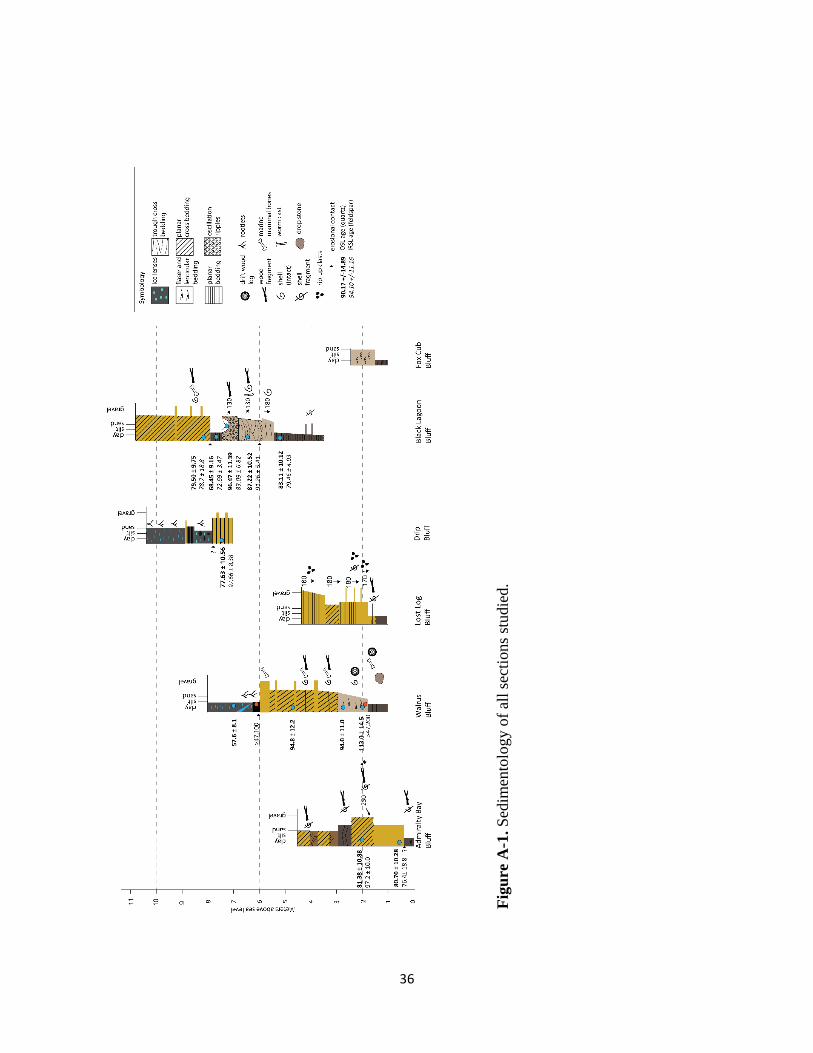
36
Fig
ure
A-1
. S
edim
ento
logy o
f al
l se
ctio
ns
studie
d.

37
Figure A-2.Walrus Bluff with designated units and OSL ages. Note that photo was taken before
the section covering OSL sample from Unit 4 was excavated and cleaned.
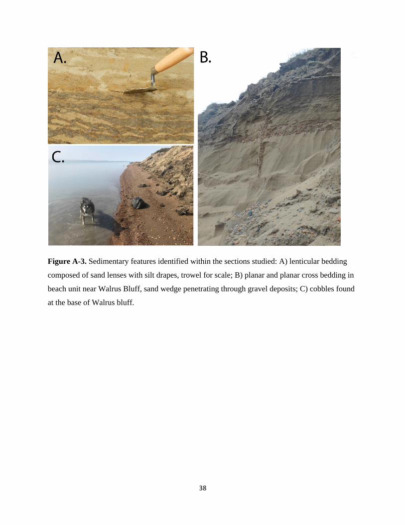
38
Figure A-3. Sedimentary features identified within the sections studied: A) lenticular bedding
composed of sand lenses with silt drapes, trowel for scale; B) planar and planar cross bedding in
beach unit near Walrus Bluff, sand wedge penetrating through gravel deposits; C) cobbles found
at the base of Walrus bluff.

39
Figure A-4. A sub-sample of fossils found in-situ: A) a walrus tooth; B) bivalve Macoma
calcarean; C) Pusa hispida (ringed seal) metatarsal; D) coniferous drift-wood; E) worm hole
casts; F) Mammuthus primigenius (woolly mammoth) tusk fragment.

40
Figure A-5. OSL Equivalent dose (DE) and IRSL Age Distributions. Probability density
functions and radial plots. All references to NTB section are from Walrus Bluff.

41
Figure A-5. Continued.

42
Figure A-5. Continued.
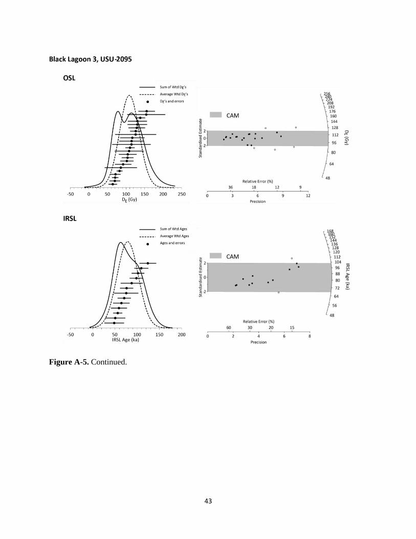
43
Figure A-5. Continued.

44
Figure A-5. Continued.

45
Figure A-5. Continued.
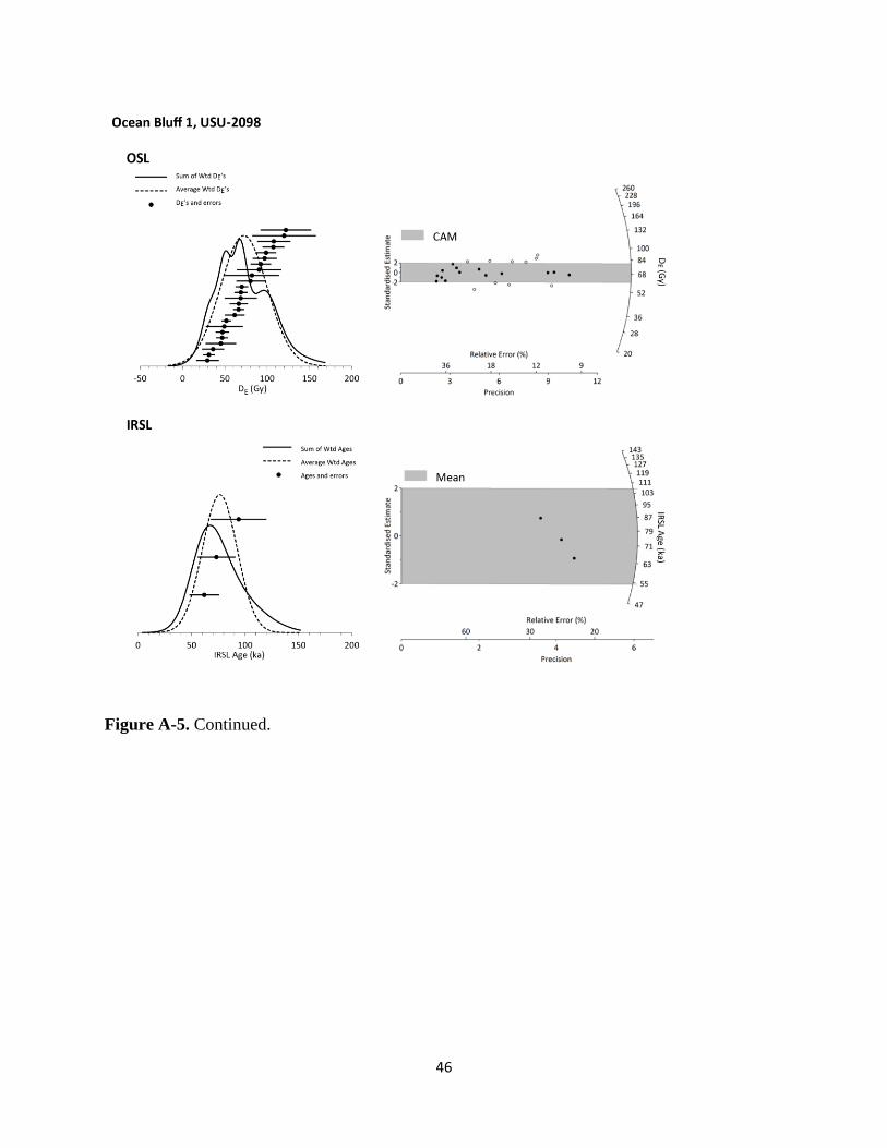
46
Figure A-5. Continued.

47
Figure A-5. Continued.

48
Figure A-5. Continued.

49
Figure A-6. Grain size composition for Fox Cub Bluff illustrating upwards coarsening as sea
level transgressed.

50
Table A-1: Locations of sections sampled
Section Latitude Longitude
Admiralty Bay 70.93° -155.51°
Walrus 70.72° -153.72°
Drip 70.72° -153.71°
Black Lagoon 70.72° -153.56°
Fox Cub 70.72° -153.55°
Lost Log 70.72° -153.72°
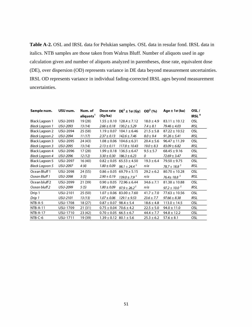
51
Table A-2. OSL and IRSL data for Pelukian samples. OSL data in resular fond. IRSL data in
italics. NTB samples are those taken from Walrus Bluff. Number of aliquots used in age
calculation given and number of aliquots analyzed in parentheses, dose rate, equivalent dose
(DE), over dispersion (OD) represents variance in DE data beyond measurement uncertainties.
IRSL OD represents variance in individual fading-corrected IRSL ages beyond measurement
uncertainties.

52
Table A-3. Geochemistry of OSL samples

53
Table A-4: Shells found at study sites that were selected for identification

54
Appendix A References
Barnes, P.W., Reimnitz, E. and Fox, D., 1982. Ice rafting of fine-grained sediment, a sorting and
transport mechanism, Beaufort Sea, Alaska. Journal of Sedimentary Research, 52(2).
Bateman, M.D. and Murton, J.B., 2006. The chronostratigraphy of Late Pleistocene glacial and
periglacial aeolian activity in the Tuktoyaktuk Coastlands, NWT, Canada. Quaternary
Science Reviews, 25(19), pp.2552-2568.
Blott, S.J. and Pye, K., 2001. GRADISTAT: a grain size distribution and statistics package for
the analysis of unconsolidated sediments. Earth surface processes and Landforms, 26(11),
pp.1237-1248.
Brigham-Grette, J. and Hopkins, D.M., 1995. Emergent marine record and paleoclimate of the
last interglaciation along the northwest Alaskan coast. Quaternary Research, 43(2), pp.159-
173.
Brigham-Grette, J., 2013. A fresh look at Arctic ice sheets. Nature Geoscience, 6, 807-808
Broecker, W.S., 1975. Climatic change: are we on the brink of a pronounced global warming?.
Science, pp.460-463.
Carter, L.D., Brigham-Grette, J. and Hopkins, D.M., 1986, April. Late Cenozoic marine
transgressions of the Alaskan Arctic coastal plain. In Correlation of Quaternary deposits and
events around the margin of the Beaufort Sea: contributions from a joint Canadian-
American workshop (pp. 21-26).
de Vernal, A., Miller, G.H. and Hillaire-Marcel, C., 1991. Paleoenvironments of the last
interglacial in northwest North Atlantic region and adjacent mainland Canada. Quaternary
International, 10, pp.95-106.
Dinter, D.A., 1985. Quaternary sedimentation of the Alaskan Beaufort shelf: Influence of
regional tectonics, fluctuating sea levels, and glacial sediment sources. Tectonophysics,
114(1), pp.133-161.
Dyke, A. and Prest, V., 1987. Late Wisconsinan and Holocene history of the Laurentide ice
sheet. Géographie physique et Quaternaire, 41(2), pp.237-263.
Ewing, M. and Donn, W.L., 1956. A theory of ice ages. Science, 123(3207), pp.1061-1066.

55
Forman, S.L., Pierson, J., Gomez, J., Brigham-Grette, J., Nowaczyk, N.R. and Melles, M., 2007.
Luminescence geochronology for sediments from Lake El’gygytgyn, northeast Siberia,
Russia: constraining the timing of paleoenvironmental events for the past 200 ka. Journal of
Paleolimnology, 37(1), pp.77-88.
Hopkins, D.M., 1967. The Cenozoic history of Beringia—a synthesis. In: Hopkins, D.M., (Ed)
The Bering land bridge (Vol. 3). Stanford University Press.
Kanevskiy, M., Shur, Y., Jorgenson, M.T., Ping, C.L., Michaelson, G.J., Fortier, D., Stephani,
E., Dillon, M. and Tumskoy, V., 2013. Ground ice in the upper permafrost of the Beaufort
Sea coast of Alaska. Cold Regions Science and Technology, 85, pp.56-70.
Kaufman, D.S. and Brigham-Grette, J., 1993. Aminostratigraphic correlations and
paleotemperature implications, Pliocene-Pleistocene high-sea-level deposits, northwestern
Alaska. Quaternary Science Reviews, 12(1), pp.21-33.
Mangerud, J. and Svendsen, J.I., 1992. The last interglacial-glacial period on Spitsbergen,
Svalbard. Quaternary Science Reviews, 11(6), pp.633-664.
Mercer, J.H., 1970. A former ice sheet in the Arctic Ocean?. Palaeogeography,
Palaeoclimatology, Palaeoecology, 8(1), pp.19-27.
Miller, G.H. and Brigham-Grette, J., 1989. Amino acid geochronology: resolution and precision
in carbonate fossils. Quaternary International, 1, pp.111-128.
Murton, J.B., Frechen, M. and Maddy, D., 2007. Luminescence dating of mid-to Late
Wisconsinan aeolian sand as a constraint on the last advance of the Laurentide Ice Sheet
across the Tuktoyaktuk Coastlands, western Arctic Canada. Canadian Journal of Earth
Sciences, 44(6), pp.857-869.
Reimnitz, E. and Barnes, P.W., 1987. Sea-ice influence on Arctic coastal retreat. In Coastal
Sediments' 87, Proceedings of a Specialty Conference on Advances in Understanding of
Coastal Sediment Processes. (Vol. 2, pp. 1578-1591).
Rodeick, C.A., 1979, The origin, distribution, and depositional history of gravel deposits on the
Beaufort Sea continental shelf, Alaska (No. 79-234). US Geological Survey.
Ward, B.C., Bond, J.D. and Gosse, J.C., 2007. Evidence for a 55–50 ka (early Wisconsin)
glaciation of the Cordilleran ice sheet, Yukon Territory, Canada. Quaternary Research,
68(1), pp.141-150.

56

57
Chapter 3 Spatial distribution of thermokarst terrain in Arctic Alaska2
3.1 Abstract
In landscapes underlain by ice-rich permafrost, the development of thermokarst landforms can have
drastic impacts on ecosystem processes and human infrastructure. Here we describe the distribution
of thermokarst landforms in the continuous permafrost zone of Arctic Alaska, analyze linkages to the
underlying surficial geology, and discuss the vulnerability of different types of landscapes to future
thaw. We identified nine major thermokarst landforms and then mapped their distributions in twelve
representative study areas totaling 300-km2. These study areas differ in their geologic history,
permafrost-ice content, and ground thermal regime. Results show that 63% of the entire study area is
occupied by thermokarst landforms and that the distribution of thermokarst landforms and overall
landscape complexity varies markedly with surficial geology. Areas underlain by ice-rich marine silt
are the most affected by thermokarst (97% of total area), whereas areas underlain by glacial drift are
least affected (14%). Drained thermokarst-lake basins are the most widespread thermokarst
landforms, covering 33% of the entire study region, with greater prevalence in areas of marine silt
(48% coverage), marine sand (47%), and aeolian silt (34%). Thermokarst-lakes are the second most
common thermokarst landform, covering 16% of the study region, with highest coverage in areas
underlain by marine silt (39% coverage). Thermokarst troughs and pits cover 7% of the study region
and are the third most prevalent thermokarst landform. They are most common in areas underlain by
deltaic sands and gravels (18% coverage) and marine sand (12%). Alas valleys are widespread in
areas of aeolian silt (14%) located in gradually sloping uplands. Areas of marine silt have been
particularly vulnerable to thaw in the past because they are ice-rich and have low-gradient topography
facilitating the repeated development of thermokarst-lakes. In the future, ice-rich aeolian, upland
terrain (yedoma) will be particularly susceptible to thaw because it still contains massive
concentrations of ground ice in the form of syngenetic ice-wedges that have remained largely intact
since the Pleistocene.
2 Farquharson, L.M., Mann, D.H., Grosse, G., Jones, B.M. and Romanovsky, V.E., 2016. Spatial
distribution of thermokarst terrain in Arctic Alaska. Geomorphology, 273, pp.116-133.
58
3.2. Introduction
Over the past 14,000 years of post-glacial times, one of the main geomorphic processes operating
in Arctic lowlands has been the thaw of ice-rich permafrost leading to the formation of
thermokarst topography (Czudek and Demek, 1970; Burn, 1992; Jorgenson et al., 2008a; Grosse
et al., 2013). Thermokarst, defined as surface subsidence caused by the melting of massive ice
(van Everdingen, 2005), can have pervasive effects on hydrological and ecological processes
(Kokelj et al., 2005; Myers-Smith et al., 2007), including the carbon cycle (Grosse et al., 2011).
In addition to thermokarst, other thaw-related processes include thermo-erosion (thermal and
mechanical erosion by water), thermo-denudation (thaw of sediment subaerially and its
subsequent transport by gravity), and thermo-abrasion (the thaw and transport of material by
wave action; Are, 1978; Washburn, 1979; van Everdingen, 2005). Here the term thermokarst,
refers to the topography and landforms developed after the melting of ground ice by any of the
aforementioned processes.
In Arctic Alaska, the region north of the Brooks Range underlain by continuous permafrost
(Figure 3.1), lowland substrates are commonly ice rich, with total volumetric ice contents
ranging from 40 to 90% (Kanevskiy et al., 2013). These high ice contents make the ground
vulnerable to thermal disturbance and development of thermokarst terrain. These landforms are
diverse: 23 different types have been identified based on topography and hydrology in Arctic
Alaska alone (Jorgenson et al., 2008a; Kokelj and Jorgenson, 2013).
A number of previous studies have mapped the spatial distribution of thermokarst landforms in
arctic lowlands. In Canada, these include thermokarst-lakes (Côté and Burn, 2002; Olthof et al.,
2015), active-layer detachment slides (Lewkowicz and Harris, 2005; Lamoureux and Lafreniére,
2009), retrogressive thaw slumps (Lantuit and Pollard, 2008; Lantz and Kokelj, 2008; Kokelj et
al., 2009), and degrading ice-wedges (Steedman et al., 2016). In Alaska (Table 2), mapping has
focused mainly on the spatial distribution of thermokarst-lakes and drained thermokarst-lake
basins (Frohn et al., 2005; Hinkel et al., 2005; Jones et al., 2011; Jones and Arp, 2015) and to a
lesser extent beaded streams (Arp et al., 2015), retrogressive thaw slumps (Balser et al., 2014),
and ponds formed by degrading ice-wedges (Raynolds et al., 2014; Jorgenson et al., 2015;
Liljedahl et al., 2016). In Siberia, Veremeeva and Gubin, (2009) identified a number of

59
landscape typologies in the Kolyma River lowlands including upland yedoma and alases. Other
mapping in Siberia has quantified thermokarst-lake and drained thermokarst-lake basin
distribution in yedoma regions (Grosse et al., 2008; Morgenstern et al., 2011).
The combination of ice-rich permafrost and a rapidly warming climate makes Arctic Alaska an
interesting and topical place to study the geomorphic patterns and processes of thermokarst
development. Mean annual air temperature (MAAT) at Point Barrow has increased by ~ 3°C
since 1950 (Wendler et al., 2010), and borehole measurements of ground temperatures indicate
permafrost has warmed as much as 4°C across the region during recent decades (Romanovsky et
al., 2010; Romanovsky et al., 2015; Smith et al., 2010). Warming over the coming century is
expected to be the greatest at high latitudes (Cohen et al., 2014), and MAAT in the Arctic is
projected to rise as much as 8.3°C (IPCC, 2013).
Ongoing warming has already led to a noticeable increase in thermokarst development in some
parts of Arctic Alaska (Jorgenson et al., 2006; Raynolds et al., 2014; Jorgenson et al., 2015;
Liljedahl et al., 2016), and we know from paleorecords that warming climate can trigger rapid
and widespread thawing of permafrost (Mann et al., 2010; Gaglioti et al., 2014). Short-lived
ecological disturbances in conjunction with longer-term warming trends can also trigger
thermokarst. For example, wildfires are projected to increase in frequency, intensity, and extent
in Arctic Alaska as climate warms there (Hu et al., 2015). Burning removes the organic mat that
insulates the ground and buffers the permafrost from warming surface conditions (Jones et al.,
2015).
To predict landscape-scale responses to ongoing climatic warming in the Arctic, we need to
better understand what factors control thermokarst development there. With this goal in mind,
we use remotely sensed imagery to map thermokarst landforms and quantitatively characterize
how geological substrate and topography interact with the content and structure of ground ice to
determine the incidence, morphology, and distribution of thermokarst landforms that have
developed in Arctic Alaska in post-glacial times. Our results provide a basis for predicting how
thaw-related, geomorphic processes may respond to climate warming during the coming century.

60
3.3. Study region
Our 12 study areas are located on the Arctic Coastal Plain, in the Arctic Foothills, and in the
Brooks Range (Wahrhaftig, 1965; Figure 3.1). We selected these study areas to be representative
examples of the landscapes within which they occur. The number of study areas per type of
surficial geology corresponds roughly to how widely this geological substrate is distributed in
the study region (Figure 3.1, Table 3.1). Detailed mapping was conducted in six types of surficial
geologies: aeolian silt, aeolian sand, marine silt, marine sand, glacial drift, and deltaic sand and
gravel (Jorgenson et al., 2008b). All of the study areas are underlain by continuous permafrost
(Figure 3.2). All sites except those in the Brooks Range are in areas that remained unglaciated
during the last glacial maximum (ca. 21,000 YBP (years before present). The permafrost
temperature data (for the period 1999 to 2011) used in this study were obtained from the U.S.
Geological Survey and the University of Alaska Geophysical Institute Permafrost Laboratory
(Romanovsky et al., unpublished data; Figure 3.2, Table A.3.2). Permafrost temperature stations
(shown in Figure 3.1) do not coincide directly with our study areas but are located within the
same surficial geology units. Mean annual (calendar year) values for ground temperature are
calculated using mean daily data from each site.
3.3.1. Arctic Coastal Plain: Deltaic sands and gravels
Deltaic sands and gravels cover 2% of the study region (Figure 3.1, Table 3.1). Representative of
these deposits, study area A (Figure 3.1) is located on the Ikpikpuk River delta where the
surficial geology is characterized by fine-grained, overbank deposits along with two types of
channel deposits: sandy riverbed and lateral-accretion deposits (Shur and Jorgenson, 1998). The
mean slope of the ground surface on the Ikpikpuk Delta is 0.04° (Table 3.1, all slope values
represent regional mean slope, see section 3.2). Once delta channels are abandoned, epigenetic
and syngenetic permafrost aggrades and ice-wedge polygons form. Total volumetric ice contents
in these deposits vary widely but average 70% in areas of syngenetic ice-wedges (Shur and
Jorgenson, 1998). The Ikpikpuk delta probably dates to the mid-Holocene when relative sea level
stabilized. Most of the delta surface is either barren or vegetated by pioneering herbaceous
vegetation such as Salix alaxensis, Salix lanata, and Carex aquatilis (Jorgenson et al., 1998). No
permafrost temperature data are available for this surficial geology type.

61
3.3.2 . Arctic Coastal Plain: marine silt
Study area B (Figure 3.1) is situated on marine silt, which was deposited during the most recent
marine transgression affecting the Arctic Coastal Plain during the Simpsonian interstadial ca.
75,000 cal. YBP when relative sea level was ~ 7 m higher than today (Dinter et al., 1990).
Marine silt covers 4% of the overall study region (Figure 3.1) and is limited to outer portions of
the Arctic Coastal Plain. The land surface here is basically flat with a mean slope of only 0.03°
(Table 3.1). At Drew Point (Figure 3.2), permafrost temperatures at 1.2 m depth averaged -8.0°C
between 1999 and 2010 and have increased by 0.6°C over this period. At marine-silt sites, total
volumetric ice content reaches 86% (Kanevskiy et al., 2013), and vegetation is moist acidic
tundra composed of wetland sedges, Carex aquatilis and Eriophorum angustifolium, and mosses,
Drepanocladus brevifolius, and Limprichtia revolvens (Raynolds et al., 2006).
3.3.3. Arctic Coastal Plain: marine sand
Study areas C, D, E, and F are located in areas underlain by marine sand (Figure 3.1). In total,
marine sand underlies 33% of the study region, and these areas have a mean slope of 0.10°
(Table 3.1). This sand was deposited during multiple marine transgressions of Pleistocene and
Pliocene age (Dinter et al., 1990). Permafrost temperatures at 1.2 m depth averaged -7.3°C
between 1999 and 2010 and increased by 0.8° C during this period (Figure 3.2, Fish Creek and
South Meade sites). At the marine-sand sites, total volumetric ice content averages 80%
(Kanevskiy et al., 2013), and vegetation is moist acidic tundra composed of wetland sedge,
Carex aquatilis and Eriophorum angustifolium, mosses, Drepanocladus spp. and Sphagnum
spp., and dwarf shrubs, Dryas integrifolia and Salix reticulata (Raynolds et al., 2006).
3.3.4. Arctic Coastal Plain: aeolian sand
The aeolian sand sites (G, H, and I; Figure 3.1) are located along the southern margin of the
Arctic Coastal Plain in the area of the now stabilized Ikpikpuk Sand Sea (Carter, 1981; Galloway
and Carter, 1993). Here late Pleistocene and early Holocene deposits of aeolian sand reach up to
30 m in thickness. The former Ikpikpuk Sand Sea is characterized by stabilized longitudinal and
parabolic sand dunes covering >15,000-km2 of the Arctic Coastal Plain. The last period of
widespread aeolian activity was 8000–11,000 cal. YBP (Carter, 1981; Dinter et al., 1990). Since
this time, reactivation has occurred only intermittently and locally. Altogether, aeolian sand
62
covers 23% of the study region (Figure 3.1, Table 3.1), and the mean slope of the area blanketed
by aeolian sand is 0.10° (Table 3.1). Mean permafrost temperatures at 1.2 m depth in the former
sand sea were -5.9°C between 1999 and 2010, and they increased 0.8° C during this period
(Figure 3.2, site Inigok). The average volumetric ice content here reaches 43% (Kanevskiy et al.,
2013), which is slightly greater than the typical porosity of frozen sands. At aeolian sand sites,
vegetation cover is primarily moist, nonacidic tundra composed of sedge: Eriophorum
vaginatum, dwarf shrubs, Ledum palustre, Vaccinium vitis-idaea, Cassiope tetragona, and Rubus
chamaemorus, and mosses, Sphagnum compactum, Aulacomnium turgidum, and usually lacks
any peat accumulation (Raynolds et al., 2006).
3.3.5 Arctic Foothills: aeolian silt (yedoma)
Study areas J and K are located in a belt of ice-rich silt (yedoma) lying along the southern margin
of the Ikpikpuk Sand Sea and north of previously glaciated terrain (Figure 3.1). Yedoma is
organic-rich silt (loess) deposited during the late Pleistocene. It typically contains large,
syngenetic ice-wedges (Kanevskiy et al., 2011). In total, yedoma covers 35% of the study region
(Figure 3.1), and the mean slope of the yedoma zone is 0.32° (Table 3.1). Mean permafrost
temperatures at 1.2 m depth were -5.2°C between 1999 and 2010, and permafrost temperature
increased by as much as 1.0°C during this period (Figure 3.2, sites Koluktak and Umiat).
Deposition of yedoma mainly took place during the late Pleistocene, and it accumulated up to 50
m thick in some areas of Beringia (Schirrmeister et al., 2013). Within our study area, yedoma is
characterized by a high total volumetric ice content of 89%, mainly because of the presence of
syngenetic ice-wedges (Kanevskiy et al., 2011). Vegetation cover is moist acidic tundra
characterized by sedges, Carex bigelowii, and Eriophorum angustifolium, dwarf shrubs, Dryas
integrifolia and Salix reticulata, forbes, Tephroseris frigida, and Eutrema edwardsii, and mosses,
Drepanocladus brevifolius and Distichium capillaceum (Raynolds et al., 2006).
3.3.6. Brooks Range: glacial drift
Study area L is located in the Brooks Range where four glacial advances, the most recent
between 24,000 and 17,000 cal. yr BP, have left behind a complex surficial geology (Hamilton,
2003; Figure 3.1). In total, glacial drift covers 2% of the study region (Figure 3.1), and these
areas have a mean slope of 2.04° (Table 1). Permafrost temperatures at 1.0 m depth are the

63
warmest of all the surficial geology types, averaging -4.6°C for the period 2000 to 2011 (Figure
3.2, Galbraith). These ground temperatures increased by 1.5°C between 2000 and 2011.
Thermokarst landforms in this area have developed mainly from the melting of buried glacial ice
bodies (Hamilton, 2003), augmented by the melting of Holocene-aged ice wedges. Thermokarst-
lakes within this substrate type can also be termed kettle lakes in cases where they formed from
the thaw and collapse of buried glacial ice. Vegetation is nonacidic tundra composed of sedges,
Eriophorum vaginatum and Carex bigelowii, dwarf shrubs, Betula nana; Ledum palustre,
Vaccinium vitis-idaea, and mosses, Sphagnum spp., and Hylocomium splendens (Reynolds et al.,
2006).
3.4. Methods
3.4.1 Definition of thermokarst landforms
We selected study areas of contrasting surficial geology and ground-ice content based on the
mapping of Jorgenson et al. (2008b). The study areas are representative of the terrain and
surficial geology types occurring in Arctic Alaska.
We mapped nine different thermokarst landforms, all of which are familiar in the periglacial
literature (French, 2007; Jorgenson, 2013; Soloviev, 1973), with the exception of flooded ice-
wedge polygons and thaw valleys. The landforms in this study are not the only ones existing in
Arctic Alaska, but they are the main ones. Five of the thermokarst landforms are large features
(>50 m2): thermokarst-lakes, drained thermokarst-lake basins, alas valleys (Soloviev, 1973;
Goudie, 2004), thaw valleys, and retrogressive thaw slumps. Four of the thermokarst landforms
are relatively small features (<50 m2): beaded stream ponds, drained thaw-ponds, thermokarst
troughs and pits, and flooded ice-wedge polygons (Figure 3.3). Most thermokarst landforms
were identified according to the visual characteristics and spatial dimensions described by
Jorgenson et al. (2008a) and Jorgenson (2013). Drained thaw-ponds were identified aerially and
during field surveys on the basis of pools of standing water, drowned vegetation, and concentric
vegetation zonation suggesting variable water levels in the past. We used the descriptions of
Soloviev (1973) to identify alas and thaw valleys. We classify alas and thaw valleys together, as

64
they exhibit the same morphology — thermokarst-lake basins connected by valleys or valley-like
features — but the term “alas valley” specifically refers to yedoma regions.
3.4.2. Mapping of thermokarst landforms
Thermokarst landforms (Figure 3.3) were mapped in twelve 25-km2 study areas (Figs. 3.1, 3.4).
We delineated landforms by manually digitizing features using 2.5-m resolution, false color,
infrared, aerial-image orthophotography (July, August, 2002-2006) for all sites except L, for
which we used 0.3-m resolution World View 2 imagery. An IfSAR DSM (Inferometic Synthetic
Aperture Radar Digital Surface Model) was also used for all sites. Raw IfSAR data were
collected by Intermap Technologies using a STAR-3i airborne synthetic aperture radar system
(high-resolution, single pass) in summers between 2002 and 2006 (Intermap, 2010). IfSAR DSM
tiles were used to create a raster mosaic of the study areas with a horizontal resolution of 5 m and
a vertical resolution of 1 m. Bluff heights were calculated using the IfSAR DSM. Elevation
ranges were assessed for individual landforms within a 50-m buffer around the feature. Slope
data were calculated using the Scenarios Network for Alaska (SNAP) 1-km resolution Alaska
slope model (http://ckan.snap.uaf.edu/dataset/slope). To estimate slope angles, we used 1-km
resolution slope data, because the 5-m resolution, IfSAR slope data are affected by small-scale
topographic features. For water bodies, we used the water and lake/river ice classes used in the
National Land Cover Database (Homer et al., 2015), which is based on classification of 2001–
2011 Landsat-5 Thematic Mapper data at 30-m resolution, which allows us to map all lakes >1
ha. Landforms were manually digitized in ArcMap v.10.0 (ESRITM) software (see Grosse et al.,
2006; Morgenstern et al., 2011) at a scale of 1:2000. Landform metrics data were also calculated
using ArcMap. To assess the accuracy of landform mapping, we conducted ground surveys of all
12 study areas in the summer of 2013. Qualitative surveys were conducted on foot, using maps
overlain by our landform classification. In addition, all five authors have spent considerable time
in the area, conducting geomorphic research, on foot and during low-elevation flight surveys.
We adhered to set rules when mapping complicated landforms. For instance, landform
boundaries were manually delineated around clusters of thermokarst troughs and pits and flooded
polygons exhibiting similar degradation and ponding characteristics. Beaded streams were
digitized as polylines and then buffered with a width of 90 m (Arp et al., 2015) using the buffer

65
analysis tool in ArcGIS. Multi-basin lakes and drained-lake basins were divided into individual
lakes when the basins exhibited roughly an hourglass shape indicative of coalescence. In site A
(Ikpikpuk Delta), active river channels were masked at the water line and not included in land-
cover calculations. Landform density was calculated by counting the number of each landform
type present in each study area, then dividing by the area affected by thermokarst.
3.4.3 Classification of terrain as ‘currently active thermokarst’ or ‘previously active
thermokarst’
We used the spectral characteristics of vegetation cover and liquid water to classify thermokarst
landforms as either currently active or previously active. In addition, we mapped areas that had
no observable thermokarst landforms. Currently thermokarst affected landforms are those under
the influence of thermokarst processes at the time of image acquisition. In the case of
thermokarst trough and pit zones and thermokarst-lakes, we interpreted the presence of standing
water pits and troughs as indicative of active thermokarst, which may lead to underestimating the
extent of these features in areas with good drainage. In the case of beaded channels, we
interpreted the presence of water as a probable indicator of talik (thaw bulb) presence. All alas
and thaw valleys had low reflectivity values associated with landscape wetting and/or showed
signs of strong ice-wedge degradation and ponding at the head of the channel system.
Currently inactive landforms are those not actively developing at the time of image acquisition.
Vegetation cover was used as a key indicator of geomorphic stability. Vegetated retrogressive
thaw slump scars were classified as currently inactive thermokarst terrain. Areas classified as
non-thermokarst-affected were those where no evidence of either current or past thermokarst
activity was detected.
We quantified the extent of repeated ice aggradation and subsequent thaw across the landscape
by determining the number of overlapping generations of thermokarst-lakes (Billings and
Peterson, 1980; Jones et al., 2012). We mapped the cross-cutting relationships of multiple
thermokarst-lakes using the outlines of former basins where they were visible and extrapolating
the likely location of lake margins that had been destroyed by subsequent lake generations. To
make such extrapolations, we assume these lakes tend to have circular or elliptical shapes.

66
3.5. Results
3.5.1. Distribution of thermokarst landforms in relation to surficial geology
3.5.1.1. Deltaic sands and gravels
On the Ikpikpuk delta (site A), 37% of the landscape has been affected by thermokarst processes
(Figs. 3.4, 3.5, 3.6, Table 3.3). The most widely distributed landforms are thermokarst troughs
and pits, which cover 18% of the total area (Figure 3.5, Table 3.3). Individual groupings of
thermokarst troughs and pits have an average area of 3.7 ha (Table 3.4). Small lakes (mean area
8.1 ha; Table 3.4) cover 13% of the study area. Mean elevation range is 4.7 m (Table 3.4). This
study area has a landform density of 14.5 landforms per km2 (Figure 3.7). No drained
thermokarst-lake basins were observed, and all thermokarst landforms observed are currently
classified as active (Figure 3.6).
3.5.1.2. Areas of marine silt
The extent of thaw-affected terrain is greatest on the northern Arctic Coastal Plain where ice-rich
marine silt is present (site B). Here, thermokarst has modified 97% of the landscape (Figs. 3.4
and 3.6, Table 3.3). Three percent of the area was unclassified because of the presence of small
water bodies less than 1 ha in size situated within drained thermokarst-lake basins. Drained
thermokarst-lake basins and thermokarst-lakes are the dominant thermokarst landforms, covering
48 and 39% respectively of the study area (Figure 3.5, Table 3.3). These basins and lakes have
mean surface areas of 232 and 110 ha, respectively (Table 3.4). Mean bluff height is relatively
low for thermokarst-lakes and drained thermokarst-lake basins, only 3.5 and 5.3 m, respectively
(Table 3.4). Up to four generations of drained-lake basins are present in addition to existing
thermokarst-lakes (Figure 3.8). In this study area, a single zone of thermokarst troughs and pits is
perched on an upland area comprising 9% of the total study area. Four types of thermokarst
landforms are present, which yields a relatively low landform density of 0.9 per km2 (Figure 3.7).
A low landform density combined with a high percentage of thermokarst cover results from few
landforms that are relatively large in size. When grouped into currently and previously active
landforms, 48% of study area B is comprised of previously active landforms and 48% by
currently active landforms (Figure 3.6).
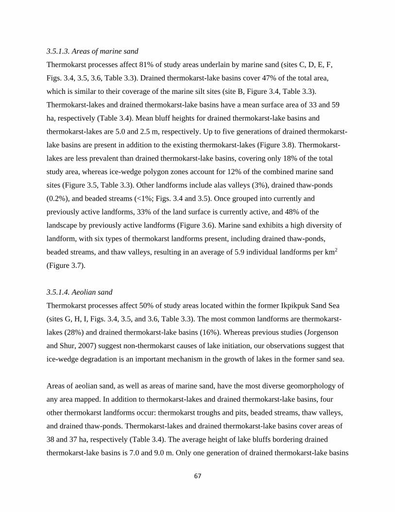
67
3.5.1.3. Areas of marine sand
Thermokarst processes affect 81% of study areas underlain by marine sand (sites C, D, E, F,
Figs. 3.4, 3.5, 3.6, Table 3.3). Drained thermokarst-lake basins cover 47% of the total area,
which is similar to their coverage of the marine silt sites (site B, Figure 3.4, Table 3.3).
Thermokarst-lakes and drained thermokarst-lake basins have a mean surface area of 33 and 59
ha, respectively (Table 3.4). Mean bluff heights for drained thermokarst-lake basins and
thermokarst-lakes are 5.0 and 2.5 m, respectively. Up to five generations of drained thermokarst-
lake basins are present in addition to the existing thermokarst-lakes (Figure 3.8). Thermokarst-
lakes are less prevalent than drained thermokarst-lake basins, covering only 18% of the total
study area, whereas ice-wedge polygon zones account for 12% of the combined marine sand
sites (Figure 3.5, Table 3.3). Other landforms include alas valleys (3%), drained thaw-ponds
(0.2%), and beaded streams (<1%; Figs. 3.4 and 3.5). Once grouped into currently and
previously active landforms, 33% of the land surface is currently active, and 48% of the
landscape by previously active landforms (Figure 3.6). Marine sand exhibits a high diversity of
landform, with six types of thermokarst landforms present, including drained thaw-ponds,
beaded streams, and thaw valleys, resulting in an average of 5.9 individual landforms per km2
(Figure 3.7).
3.5.1.4. Aeolian sand
Thermokarst processes affect 50% of study areas located within the former Ikpikpuk Sand Sea
(sites G, H, I, Figs. 3.4, 3.5, and 3.6, Table 3.3). The most common landforms are thermokarst-
lakes (28%) and drained thermokarst-lake basins (16%). Whereas previous studies (Jorgenson
and Shur, 2007) suggest non-thermokarst causes of lake initiation, our observations suggest that
ice-wedge degradation is an important mechanism in the growth of lakes in the former sand sea.
Areas of aeolian sand, as well as areas of marine sand, have the most diverse geomorphology of
any area mapped. In addition to thermokarst-lakes and drained thermokarst-lake basins, four
other thermokarst landforms occur: thermokarst troughs and pits, beaded streams, thaw valleys,
and drained thaw-ponds. Thermokarst-lakes and drained thermokarst-lake basins cover areas of
38 and 37 ha, respectively (Table 3.4). The average height of lake bluffs bordering drained
thermokarst-lake basins is 7.0 and 9.0 m. Only one generation of drained thermokarst-lake basins

68
occurs in addition to the existing thermokarst-lakes (Figure 3.8). Zones of thermokarst troughs
and pits cover 5% of aeolian sand areas (Table 3.3). Beaded streams, thaw valleys, and drained
thaw-ponds have similarly limited coverage. In total, 33% of aeolian sand areas are covered by
currently active landforms and 17% by previously active landforms (Figure 3.6). This leaves
some 49% of the landscape that preserves relict, sand-dune landforms and so exhibits no
evidence of either past thermokarst processes or ongoing thermokarst activity (Figure 3.6).
3.5.1.5 Areas of aeolian silt
Thermokarst processes have affected ~ 58% of the landscape in the aeolian silt (yedoma) zone of
the Arctic Foothills (sites J and K, Figs. 3.4, 3.5, and 3.6, Table 3.3). Drained thermokarst-lake
basins are the most widely distributed landform (Figure 3.5), covering 34% of the combined
study areas (Table 3.3) with a mean area of 80 ha per individual basin (Table 3.4). Mean bluff
height bordering drained thermokarst-lake basins and thermokarst-lakes is 19.3 and 11.0 m,
respectively. Some 24% of the landscape is characterized by currently active landforms and 34%
by previously active landforms (Figure 3.6). Thermokarst trough and pit zones and beaded
streams cover 4 and <1% of the total area, respectively. Zones of aeolian silt show similar
landform density to those of glacial drift, with 22 landforms per thaw-affected km2 (Figure 3.7).
Up to three generations of drained thermokarst-lake basins occur in addition to extant
thermokarst-lakes (Figure 3.8). Thermokarst-lakes have a more restricted coverage here than do
alas valleys, covering 6 and 14% of sites J and K, respectively (Table 3.3). Individual alas
valleys and thermokarst-lakes have a mean area of 12 ha (Table 3.4).
3.5.1.6. Glacial drift
Areas underlain by glacial drift exhibit the lowest percent coverage by thermokarst landforms of
any study area, only 14% (site L, Figs. 3.4, 3.5, and 3.6, Table 3.3). Within the glacial drift,
thermokarst-lakes are the dominant thermokarst landform (Figure 3.5), covering 12.6%, with a
mean area of 9 ha (n = 35; Table 3.4). The average bluff height around these lakes is 13.7 m,
likely reflecting the presence of massive, buried glacial ice in the area. Thaw slumps (observed
only on lake margins; n = 2) and beaded streams (n = 13) account for the remaining thaw-
affected area (<1%; Figure 3.5). Site L is the only study area where retrogressive thaw slump
activity occurs. This study area exhibits high spatial complexity, with 22 landforms per
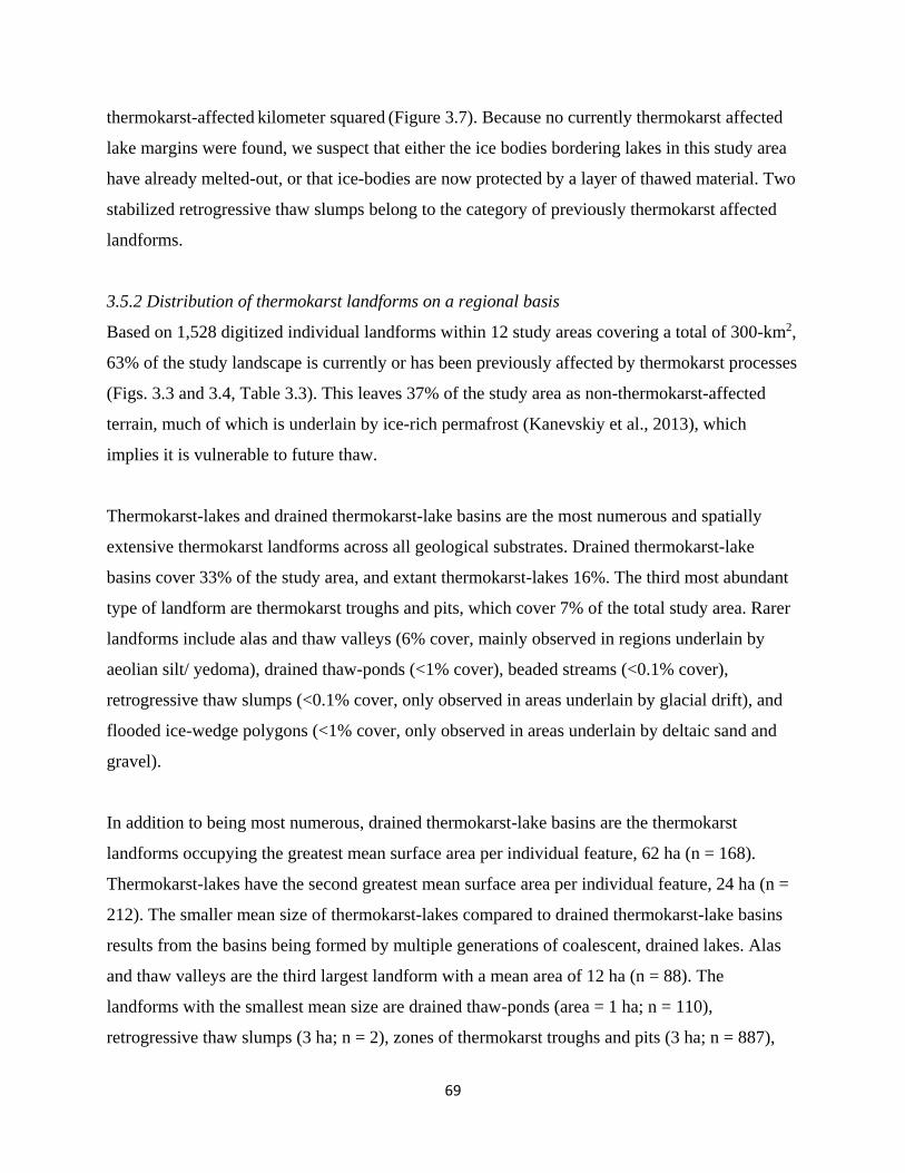
69
thermokarst-affected kilometer squared (Figure 3.7). Because no currently thermokarst affected
lake margins were found, we suspect that either the ice bodies bordering lakes in this study area
have already melted-out, or that ice-bodies are now protected by a layer of thawed material. Two
stabilized retrogressive thaw slumps belong to the category of previously thermokarst affected
landforms.
3.5.2 Distribution of thermokarst landforms on a regional basis
Based on 1,528 digitized individual landforms within 12 study areas covering a total of 300-km2,
63% of the study landscape is currently or has been previously affected by thermokarst processes
(Figs. 3.3 and 3.4, Table 3.3). This leaves 37% of the study area as non-thermokarst-affected
terrain, much of which is underlain by ice-rich permafrost (Kanevskiy et al., 2013), which
implies it is vulnerable to future thaw.
Thermokarst-lakes and drained thermokarst-lake basins are the most numerous and spatially
extensive thermokarst landforms across all geological substrates. Drained thermokarst-lake
basins cover 33% of the study area, and extant thermokarst-lakes 16%. The third most abundant
type of landform are thermokarst troughs and pits, which cover 7% of the total study area. Rarer
landforms include alas and thaw valleys (6% cover, mainly observed in regions underlain by
aeolian silt/ yedoma), drained thaw-ponds (<1% cover), beaded streams (<0.1% cover),
retrogressive thaw slumps (<0.1% cover, only observed in areas underlain by glacial drift), and
flooded ice-wedge polygons (<1% cover, only observed in areas underlain by deltaic sand and
gravel).
In addition to being most numerous, drained thermokarst-lake basins are the thermokarst
landforms occupying the greatest mean surface area per individual feature, 62 ha (n = 168).
Thermokarst-lakes have the second greatest mean surface area per individual feature, 24 ha (n =
212). The smaller mean size of thermokarst-lakes compared to drained thermokarst-lake basins
results from the basins being formed by multiple generations of coalescent, drained lakes. Alas
and thaw valleys are the third largest landform with a mean area of 12 ha (n = 88). The
landforms with the smallest mean size are drained thaw-ponds (area = 1 ha; n = 110),
retrogressive thaw slumps (3 ha; n = 2), zones of thermokarst troughs and pits (3 ha; n = 887),

70
and beaded streams (4.8 ha; n = 37). Mean elevation range of these landforms varies from 10.7 m
(beaded streams) to 2.6 m (drained thaw-ponds). Overall, beaded streams and alas and thaw
valleys exhibit the highest mean elevation ranges, 10.7 and 9.0 m, respectively (Table 3.4).
3.6. Discussion
3.6.1 Comparison with previous studies
Overall, our findings are similar to previous mapping efforts of permafrost-affected arctic
lowlands. Our cover estimates for thermokarst-lakes and drained thermokarst-lake basins in areas
of marine silt and sand align closely with previous results from the Arctic Coastal Plain of
Alaska (Frohn et al., 2005; Hinkel et al., 2005; Wang et al., 2012; Jones and Arp, 2015; Table
3.2). Mapped areas of yedoma areas in the lowlands of northern Siberia exhibit similar coverage
by thermokarst-lakes and drained thermokarst-lake basins as our study (Grosse et al., 2006,
2008; Morgenstern et al., 2011; Tables 3.2 and 3.3). Although our estimates of percent cover by
drained thermokarst-lake basin at aeolian silt sites in the Arctic Foothills (34%) agree with
previous studies in this region (Wang et al., 2012), they differ from observations in similar
substrates on the northern Seward Peninsula and in the Kolyma lowlands, where the distribution
of drained thermokarst-lake basins is much greater, around 75 (Jones et al., 2012) and 61%
(Veremeeva and Gubin, 2009) respectively. This difference may be because most thermokarst-
lakes on the Seward Peninsula have developed on a flat plain rather than in the foothills. The
mean slope for the aeolian silt region of the Arctic Foothills is 0.30° whereas the mean slope on
the Seward Peninsula lowlands is only 0.15°, which is similar to areas of marine sand in our
study area.
Finally, our results regarding beaded stream distribution generally agree with previous mapping
efforts in Arctic Alaska (Jorgenson et al., 2008b; Arp et al., 2015). Arp et al. (2015) observed a
lower distribution of beaded streams across areas of aeolian sand compared to other surficial
geology types on the Arctic Coastal Plain, a pattern also seen in this study. High ground ice
content and greater topographic relief probably favor the formation of beaded streams.

71
3.6.2 Distribution of landforms
We found that regardless of underlying surficial geology, thermokarst-lake development is the
dominant, thermokarst geomorphic process in lowland areas of Arctic Alaska, as mapped at this
point in time. Thermokarst-lake development (thermokarst-lakes and drained thermokarst-lake
basins combined) has affected 49% of the combined study areas and has been most intense in
areas of marine silt and sand (Figs. 3.4 and 3.5). These areas typically are underlain by ice-rich
permafrost and are relatively flat. In combination, both of these factors are conducive to repeated
cycles of thermokarst pit, thermokarst pond and eventual thermokarst-lake, development. In
contrast, thermokarst-lakes and drained thermokarst-lake basins are much less abundant in areas
underlain by aeolian sand, aeolian silt, glacial drift, or deltaic deposits (Figs. 3.4 and 3.5).
Though less widespread, landforms like alas and thaw valleys and thermokarst troughs and pits
are important components of Arctic Alaska’s landscape. Alas and thaw valleys are largely
restricted to areas underlain by aeolian silt, where they cover around 14% of the landscape. In
contrast, zones of thermokarst troughs and pits occur in all surficial geological types, albeit at
low densities. Altogether, zones of thermokarst troughs and pits cover ~ 7% of the combined
study areas. The only surficial-geology type where they do not occur is in glacial drift. This may
result from the pronounced topographic relief there (mean slope there is 2°) that creates good
drainage conditions that inhibit extensive ice-wedge polygon pond development. Thermokarst
troughs and pits are most extensive in areas underlain by deltaic sands and gravels and marine
sands where they cover 18 and 12%, respectively. Though not observed during this study, it is
important to note that thermokarst troughs and pits can also form within ancient drained
thermokarst-lake basins. Over hundreds to thousands of years, epigenetic ice-wedges form
within lacustrine sediments and terrestrial peat, and any disturbance to the ground thermal
regime can result in ice-wedge degradation.
Beaded stream channels cover only a small percentage of the landscape regardless of surficial
geology (0.6%). Despite their restricted occurrence, beaded streams play an important role in
sediment and nutrient transport through tundra watersheds (Arp et al., 2015).
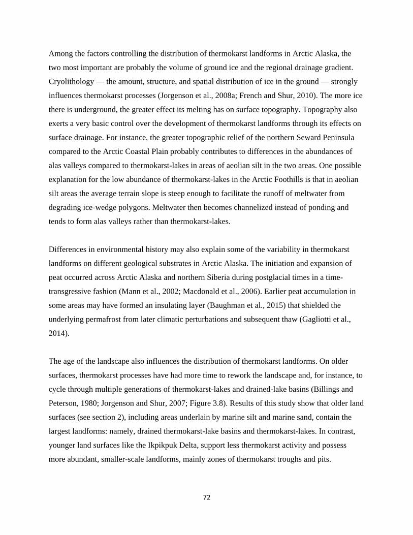
72
Among the factors controlling the distribution of thermokarst landforms in Arctic Alaska, the
two most important are probably the volume of ground ice and the regional drainage gradient.
Cryolithology — the amount, structure, and spatial distribution of ice in the ground — strongly
influences thermokarst processes (Jorgenson et al., 2008a; French and Shur, 2010). The more ice
there is underground, the greater effect its melting has on surface topography. Topography also
exerts a very basic control over the development of thermokarst landforms through its effects on
surface drainage. For instance, the greater topographic relief of the northern Seward Peninsula
compared to the Arctic Coastal Plain probably contributes to differences in the abundances of
alas valleys compared to thermokarst-lakes in areas of aeolian silt in the two areas. One possible
explanation for the low abundance of thermokarst-lakes in the Arctic Foothills is that in aeolian
silt areas the average terrain slope is steep enough to facilitate the runoff of meltwater from
degrading ice-wedge polygons. Meltwater then becomes channelized instead of ponding and
tends to form alas valleys rather than thermokarst-lakes.
Differences in environmental history may also explain some of the variability in thermokarst
landforms on different geological substrates in Arctic Alaska. The initiation and expansion of
peat occurred across Arctic Alaska and northern Siberia during postglacial times in a time-
transgressive fashion (Mann et al., 2002; Macdonald et al., 2006). Earlier peat accumulation in
some areas may have formed an insulating layer (Baughman et al., 2015) that shielded the
underlying permafrost from later climatic perturbations and subsequent thaw (Gagliotti et al.,
2014).
The age of the landscape also influences the distribution of thermokarst landforms. On older
surfaces, thermokarst processes have had more time to rework the landscape and, for instance, to
cycle through multiple generations of thermokarst-lakes and drained-lake basins (Billings and
Peterson, 1980; Jorgenson and Shur, 2007; Figure 3.8). Results of this study show that older land
surfaces (see section 2), including areas underlain by marine silt and marine sand, contain the
largest landforms: namely, drained thermokarst-lake basins and thermokarst-lakes. In contrast,
younger land surfaces like the Ikpikpuk Delta, support less thermokarst activity and possess
more abundant, smaller-scale landforms, mainly zones of thermokarst troughs and pits.

73
Older land surfaces may provide indications about the future, developmental trajectories of
younger landscapes. For instance, the relative abundance of thermokarst troughs and pits on
young surfaces may represent the initial stage of formation for other thaw-related landforms
including thermokarst-lakes (Czudek and Demek, 1970; Farquharson et al., 2016), beaded
streams (Arp et al., 2015), and in some cases, thaw-slumps (Burn and Lewkowicz, 1990).
3.6.3. Landscape vulnerability to future thaw
The vulnerability of permafrost terrain to thaw is mediated by the climate at the ground surface,
and the climate of Arctic Alaska is currently changing rapidly. In response, permafrost
temperatures are rising in all the surficial geology types we studied (Figure 3.2). The fastest rates
of warming are in the glacial drift (up to 1.5°C increase between 2000 and 2011) and in aeolian
silt areas (1.1°C increase between 1999 and 2010). Interestingly, sites with the coldest (-7.4°C)
permafrost are also the most thaw-affected, probably because they are more ice-rich than the
warmer (-3.3°C) permafrost sites. Mean annual air temperature (MAATs) is projected to increase
in the Arctic by up to 8.3°C over the coming century (see IPCC, 2013, Table 22.2), and this will
undoubtedly cause further ground temperature warming in Arctic Alaska.
Changing climate is causing an increased frequency of wildland fires in Arctic Alaska (Hu et al.,
2015). Fire is a major threat to landscape stability there because it destroys the peat layers that
insulate the ground and buffer the underlying permafrost from changes in air temperature (Mack
et al., 2011). Removal of these insulating peat layers from terrain underlain by ice-rich
permafrost can trigger drastic and widespread thermokarst (Jones et al., 2015). Our finding that
areas underlain by aeolian silt contain large areas (43%) not yet affected by thermokarst suggests
this surficial geology type possesses a relatively high degree of resistance to thaw. One possible
explanation for this resistance is that the higher slope angle of this surficial geology type
compared to most others (Table 3.3) improves drainage conditions and inhibits thermokarst.
Alternatively, the presence of extensive areas of non-thaw-affected terrain in yedoma areas may
result from an earlier spread of insulating organic soils in post-glacial times, which so far has
buffered the underlying permafrost from periods of warm temperature (Mann et al., 2010). If
true, this implies that peat-supporting yedoma areas may now be highly vulnerable to extensive
thermokarst triggered by more frequent wildland fires.
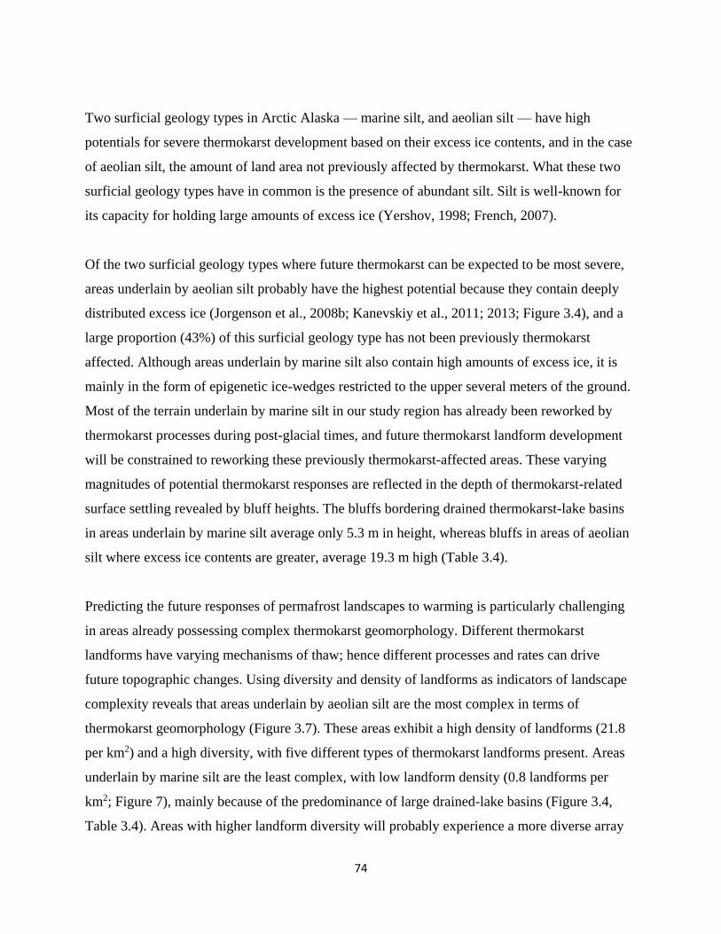
74
Two surficial geology types in Arctic Alaska — marine silt, and aeolian silt — have high
potentials for severe thermokarst development based on their excess ice contents, and in the case
of aeolian silt, the amount of land area not previously affected by thermokarst. What these two
surficial geology types have in common is the presence of abundant silt. Silt is well-known for
its capacity for holding large amounts of excess ice (Yershov, 1998; French, 2007).
Of the two surficial geology types where future thermokarst can be expected to be most severe,
areas underlain by aeolian silt probably have the highest potential because they contain deeply
distributed excess ice (Jorgenson et al., 2008b; Kanevskiy et al., 2011; 2013; Figure 3.4), and a
large proportion (43%) of this surficial geology type has not been previously thermokarst
affected. Although areas underlain by marine silt also contain high amounts of excess ice, it is
mainly in the form of epigenetic ice-wedges restricted to the upper several meters of the ground.
Most of the terrain underlain by marine silt in our study region has already been reworked by
thermokarst processes during post-glacial times, and future thermokarst landform development
will be constrained to reworking these previously thermokarst-affected areas. These varying
magnitudes of potential thermokarst responses are reflected in the depth of thermokarst-related
surface settling revealed by bluff heights. The bluffs bordering drained thermokarst-lake basins
in areas underlain by marine silt average only 5.3 m in height, whereas bluffs in areas of aeolian
silt where excess ice contents are greater, average 19.3 m high (Table 3.4).
Predicting the future responses of permafrost landscapes to warming is particularly challenging
in areas already possessing complex thermokarst geomorphology. Different thermokarst
landforms have varying mechanisms of thaw; hence different processes and rates can drive
future topographic changes. Using diversity and density of landforms as indicators of landscape
complexity reveals that areas underlain by aeolian silt are the most complex in terms of
thermokarst geomorphology (Figure 3.7). These areas exhibit a high density of landforms (21.8
per km2) and a high diversity, with five different types of thermokarst landforms present. Areas
underlain by marine silt are the least complex, with low landform density (0.8 landforms per
km2; Figure 7), mainly because of the predominance of large drained-lake basins (Figure 3.4,
Table 3.4). Areas with higher landform diversity will probably experience a more diverse array

75
of geomorphological responses to disturbances related to warming climate. Assessing the
vulnerability to future thaw in areas underlain by glacial drift and deltaic sands is particularly
challenging. Areas of glacial drift possess heterogeneous cryolithology and excess-ice content
because of the presence of buried glacial ice. The distribution of excess ice within areas of
deltaic sands is similarly unpredictable.
3.7. Conclusions
Results of this study improve understanding of future geomorphological responses to climate
change in permafrost landscapes underlain by different surficial geologies in Arctic Alaska.
Some of these results are also relevant to the ice-rich, coastal lowlands of northeast Siberia.
Thermokarst landforms are widespread in Arctic Alaska and cover 60% of the 300-km2 area we
mapped. Some of these landforms are actively forming today, while others are relict features.
Thermokarst-lakes and drained thermokarst-lake basins comprise the majority of thermokarst-
affected terrain. Alas and thaw valleys and thermokarst troughs and pits are also widespread but
occur at low densities. Permafrost temperatures are currently rising throughout Arctic Alaska,
and widespread geomorphic changes related to permafrost thaw seem inevitable. Areas of marine
silt are highly vulnerable to future thaw because they tend to be ice rich in their near surface
sediments. However, because extensive thermokarst has already occurred in this surficial
geology type over the course of the Holocene, these areas contain only limited amounts of excess
ice in their upper few meters of sediment. The most severe thermokarst will probably occur in
areas of aeolian silt (yedoma) because large expanses of these surficial geology types have not
been previously disturbed by thaw (42% of total), and they contain large amounts of ice in deep,
syngenetic ice-wedges formed during the coldest parts of the ice age.

76
Acknowledgements
LMF thanks the Arctic Landscape Conservation Cooperative and USGS Alaska Climate Science
Center-funded Alaska Integrated Ecosystem Model Project for support. GG was supported by
ERC #338335. DHM was partially supported by NSF grants ARC-0902169 and PLR-1417611.
Support for BMJ was provided by the USGS Land Change Science Program and Land Remote
Sensing Program. The Teshekpuk Lake Observatory was critical for field support. We thank
Reginald Muskett for assistance with permafrost temperature data, and Helene Genet for helpful
conversations that improved the paper. We would like to thank the editor Richard Marston,
Mikhail Kanevskiy, and three anonymous reviewers whose comments and suggestions greatly
improved the manuscript. Any use of trade, product, or firm names is for descriptive purposes
only and does not imply endorsement by the U.S. Government. Field logistics were provided in
part by grants from the Bureau of Land Management and the National Science Foundation (NSF-
PLR 1417611).
3.8 References
Are, F.E., 1978. The reworking of shorelines in the permafrost zone, In: Proceedings of the
Second International Conference on Permafrost, USSR Contribution. US National Academy
of Sciences, Washington, DC, pp. 59–62.
Arp, C.D., Jones, B.M., 2009. Geography of Alaska lake districts: identification, description, and
analysis of lake-rich regions of a diverse and dynamic state. U.S. Geol. Surv. Sci. Investig.
Rep. 2008–5215, 40.
Arp, C.D., Whitman, M.S., Jones, B.M., Grosse, G., Gaglioti, B. V., Heim, K.C., 2015.
Distribution and biophysical processes of beaded streams in Arctic permafrost landscapes.
Biogeosciences 12, 29–47.
Balser, A.W., Jones, J.B., Gens, R., 2014. Timing of retrogressive thaw slump initiation in the
Noatak Basin, northwest Alaska, USA. J. Geophys. Res. Earth Surf. 119, 1106–1120.
Baughman, C.A., Mann, D.H., Verbyla, D.L., Kunz, M.L., 2015. Soil-surface organic layers in
Arctic Alaska: Spatial distribution, rates of formation, microclimatic effects. J. Geophys.
Res. Biogeosciences. 120, 1150-1164.
Billings, W.D., Peterson, K.M., 1980. Vegetational change and ice-wedge polygons through the
thermokarst-lake cycle in Arctic Alaska. Arct. Alp. Res. 413-432.

77
Burn, C.R., 1992. Thermokarst-lakes. Can. Geogr. 36, 81–85.
Burn, C.R., Lewkowicz, A.G., 1990. Retrogressive thaw slumps. Can. Geogr. 34, 273–276.
Carter, L.D., 1981. A Pleistocene sand sea on the Alaskan arctic coastal Plain. Science 211, 381–
383.
Cohen, J., Screen, J.A., Furtado, J.C., Barlow, M., Whittleston, D., Coumou, D., Francis, J.,
Dethloff, K., Entekhabi, D., Overland, J., Jones, J., 2014. Recent Arctic amplification and
extreme mid-latitude weather. Nat. Geosci. 7, 627–637.
Côté, M.M., Burn, C.R., 2002. The oriented lakes of Tuktoyaktuk Peninsula, western arctic
coast, Canada: a GIS-based analysis. Permafr. Periglac. Process. 13, 61–70.
Czudek, T., Demek, J., 1970. Thermokarst in Siberia and its influence on the development of
lowland relief. Quat. Res. 1, 103-120
Dinter, D.A., Carter, L.D., Brigham-Grette, J., 1990. Late Cenozoic geologic evolution of the
Alaskan North Slope and adjacent continental shelves, In: The Arctic Ocean Region, The
Geology of North America 50: 459-489.
Farquharson, L.M., Anthony, K.W., Bigelow, N., Edwards, M., Grosse, G., 2016. Facies analysis
of yedoma thermokarst-lakes on the northern Seward Peninsula, Alaska. Sediment. Geol.
340, 25-37
French, H. M., 2007. The periglacial environment. John Wiley and Sons. 370 pp.
French, H.M., Shur, Y., 2010. The principles of cryostratigraphy. Earth-Science Reviews 101,
190-206.
Frohn, R.C., Hinkel, K.M., Eisner, W.R., 2005. Satellite remote sensing classification of thaw
lakes and drained thaw lake basins on the North Slope of Alaska. Remote Sens. Environ. 97,
116–126.
Gaglioti, B.V, Mann, D.H., Jones, B.M., Pohlman, J.W., Kunz, M.L., Wooller, M.J., 2014.
Radiocarbon age-offsets in an arctic lake reveal the long-term response of permafrost
carbon to climate change. J. Geophys. Res. Biogeosciences 119, 557–566.
Galloway, J.P., Carter, D. L., 1993. Late Holocene longitudinal and parabolic dunes in arctic
Alaska: Preliminary interpretations of age and paleoclimatic significance. United States
Geological Survey Bulletin 2068: 3-11.
Goudie, A., 2004. Encyclopedia of geomorphology. Vol. 2. Psychology Press, 1200 pp.

78
Grosse, G., Schirrmeister, L., Kunitsky, V.V. and Hubberten, H.W., 2005, The use of CORONA
images in remote sensing of periglacial geomorphology: an illustration from the NE
Siberian coast. Permafrost and periglacial processes, 16(2), pp.163-172.
Grosse, G., Schirrmeister, L., Malthus, T.J., 2006. Application of Landsat-7 satellite data and a
DEM for the quantification of thermokarst-affected terrain types in the periglacial Lena-
Anabar coastal lowland. Polar Res. 25, 51–67.
Grosse, G., Romanovsky, V.E., Walter, K., Morgenstern, A., Lantuit, H., Zimov, S.A., 2008.
Distribution of Thermokarst Lakes and Ponds at Three Yedoma Sites in Siberia, In: Ninth
International Conferencnce on Permafrost. Institute of Northern Engineering, University of
Alaska Fairbanks, Fairbanks, USA, pp. 551–556.
Grosse, G., Harden, J., Turetsky, M., McGuire, A.D., Camill, P., Tarnocai, C., Frolking, S.,
Schuur, E.A.G., Jorgenson, T., Marchenko, S., 2011. Vulnerability of high-latitude soil
organic carbon in North America to disturbance. J. Geophys. Res. 116, G00K06.
Grosse, G., Jones, B., Arp, C., 2013. Thermokarst-lakes, drainage, and drained basins, In:
Shroner Giardino, R., Harbor, J. (Eds.), Treatise on Geomorphology. Academic Press, San
Diego, CA, pp. 325–353.
Hamilton, T.D., 2003. Glacial geology of the Toolik Lake and upper Kuparuk River regions, In:
Walker, D.A. (Ed.), Biological Papers of the University of Alaska. p. 24.
Hinkel, K.M., Frohn, R.C., Nelson, F.E., Eisner, W.R., Beck, R.A., 2005. Morphometric and
spatial analysis of thaw lakes and drained thaw lake basins in the westernArctic Coastal
Plain, Alaska. Permafr. Periglac. Process. 16, 327–341.
Homer, C.G., Dewitz, J.A., Yang, L., Jin, S., Danielson, P., Xian, G., Coulston, J., Herold, N.D.,
Wickham, J.D., Megown, K., 2015. Completion of the 2011 National Land Cover Database
for the conterminous United States-Representing a decade of land cover change
information. Photogramm. Eng. Remote Sensing 81, 345–354.
Hu, F.S., Higuera, P.E., Duffy, P., Chipman, M.L., Rocha, A. V, Young, A.M., Kelly, R., Dietze,
M.C., 2015. Arctic tundra fires: natural variability and responses to climate change. Front.
Ecol. Environ. 13, 369–377.
Intermap, 2010. Product Handbook and Quick Start Guide, Standard Edition. Intermap, p. v 4.4.
IPCC, 2013. Climate change 2013: the physical science basis. Intergov. Panel Clim. Chang.
79
Jones, B.M., Arp, C.D., 2015. Observing a Catastrophic Thermokarst Lake Drainage in Arctic
Alaska. Permafr. Periglac. Process. 26, 119-128
Jones, B.M., Grosse, G., Arp, C.D., Jones, M.C., Walter Anthony, K., Romanovsky, V.E., 2011.
Modern thermokarst-lake dynamics in the continuous permafrost zone, northern Seward
Peninsula, Alaska. J. Geophys. Res. 116, 2005–2012.
Jones, B.M., Grosse, G., Arp, C.D., Miller, E., Liu, L., Hayes, D.J., Larsen, C.F., 2015. Recent
Arctic tundra fire initiates widespread thermokarst development. Sci. Rep. 5, 15865
Jones, M.C., Grosse, G., Jones, B.M., Walter Anthony, K.M., 2012. Peat accumulation in a
thermokarst-affected landscape in continuous ice-rich permafrost, Seward Peninsula,
Alaska. J. Geophys. Res. – Biogeosciences. 117(G2).
Jorgenson, M. T., 2013. Thermokarst terrains, In: Treatise on Geomorphology, Vol 8, Glacial
and Periglacial Geomorphology, edited by: Shroder, J.F. (Ed.), Giardino, R., Harbor, J.
(Vol. Eds.), Academic Press, San Diego, 313–324.
Jorgenson, M.T., Shur, Y., 2007. Evolution of lakes and basins in arctic Alaska and discussion of
the thaw lake cycle. J. Geophys. Res. Earth Surf. 112(F2).
Jorgenson, M. T., Shur, Y. L., Walker, H. J., 1998. Evolution of a permafrost-dominated
landscape on the Colville River Delta, northern Alaska. In: Lewkowicz, A.G., Allard, M.,
(Eds.), Seventh International Conference on Permafrost. Collection Nordica, Yellowknife,
Canada pp. 523-529.
Jorgenson, M.T., Shur, Y.L., Pullman, E.R., 2006. Abrupt increase in permafrost degradation in
Arctic Alaska. Geophys. Res. Lett. 33.
Jorgenson, M.T., Shur, Y.L., Osterkamp, T.E., 2008a. Thermokarst in Alaska, In: Kane, D.L.,
Hinkel (Eds.), Ninth International Conference on Permafrost. Institute of Northern
Engineering, University of Alaska Fairbanks, Fairbanks, Alaska, pp. 869–876.
Jorgenson, M.T., Yoshikawa, K., Kanevskiy, M., Shur, Y., Romanovsky, V.E., Marchenko, S.,
Grosse, G., Brown, J., Jones, B., 2008b. Permafrost Characteristics of Alaska – A new
permafrost map of Alaska, In: Kane, D.L., Hinkel, K.M. (Eds.), Ninth International
Conference on Permafrost. Institute of Northern Engineering, University of Alaska
Fairbanks, Fairbanks, Alaska, pp. 551–556.

80
Jorgenson, T., Kanevskiy, M.Z., Shur, Y., Moskalenko, N.G., Brown, D.R.N., Wickland, K.,
Striegl, R., Koch, J., 2015. Ground ice dynamics and ecological feedbacks control ice-
wedge degradation and stabilization. JGR Earth Surface 120 (11): 2280-2297.
Kanevskiy, M., Shur, Y., Fortier, D., Jorgenson, M.T., Stephani, E., 2011. Cryostratigraphy of
late Pleistocene syngenetic permafrost (yedoma) in arctic Alaska, Itkillik River exposure.
Quat. Res. 75, 584–596.
Kanevskiy, M., Shur, Y., Jorgenson, M.T., Ping, C.L., Michaelson, G.J., Fortier, D., Stephani,
E., Dillon, M., Tumskoy, V., 2013. Ground ice in the upper permafrost of the Beaufort Sea
coast of Alaska. Cold Reg. Sci. Technol. 85, 56–70.
Kokelj, S.V, Jenkins, R.E., Milburn, D., Milburn, D., Burn, C.R., Snow, N.B., Burn, C.R., Snow,
N., 2005. The influence of thermokarst disturbance on the water quality of small upland
lakes, Mackenzie Delta region, Northwest Territories, Canada. Permafr. Periglac. Process.
16, 343–353.
Kokelj, S.V., Lantz, T.C., Kanigan, J., Smith, S.L., Coutts, R., 2009. Origin and polycyclic
behaviour of tundra thaw slumps, Mackenzie Delta region, Northwest Territories, Canada.
Permafr. Periglac. Process. 20, 173–184.
Kokelj, S.V., Jorgenson, M.T., 2013. Advances in Thermokarst Research. Permafrost and
Periglacial Processes 24, 108–119.
Lamoureux, S.F. and Lafreniére, M.J., 2009. Fluvial impact of extensive active layer
detachments, Cape Bounty, Melville Island, Canada. Arctic, Antarct. Alp. Res. 41, 59–68.
Lantuit, H. and Pollard, W.H., 2008. Fifty years of coastal erosion and retrogressive thaw slump
activity on Herschel Island, southern Beaufort Sea, Yukon Territory, Canada.
Geomorphology 95, 84–102.
Lantz, T.C. and Kokelj, S.V, 2008. Increasing rates of retrogressive thaw slump activity in the
Mackenzie Delta region, N.W.T., Canada. Geophys. Res. Lett. 35, 1–5.
Lewkowicz, A.G. and Harris, C., 2005. Morphology and geotechnique of active-layer
detachment failures in discontinuous and continuous permafrost, northern Canada.
Geomorphology 69, 275–297.

81
Liljedahl, A.K., Boike, J., Daanen, R.P., Fedorov, A.N., Frost, G.V., Grosse, G., Hinzman, L.D.,
Iijma, Y., Jorgenson, J.C., Matveyeva, N., Necsoiu, M., Raynolds, M.K., Romanovsky, V.,
Schulla, J., Tape, K.D., Walker, D.A., Wilson, C., Yabuki, H., Zona, D., 2016. Pan-Arctic
ice-wedge degradation in warming permafrost and influence on tundra hydrology. Nat.
Geosci. 9, 312–318.
Macdonald, G.M., Beilman, D.W., Kremenetski, K. V, Sheng, Y., Smith, L.C., Velichko, A.A.,
2006. Rapid early development of circumarctic peatlands and atmospheric CH4 and CO2
variations. Science 314, 285–288.
Mack, M.C., Bret-Harte, M.S., Hollingsworth, T.N., Jandt, R.R., Schuur, E.A., Shaver, G.R.,
Verbyla, D.L., 2011. Carbon loss from an unprecedented Arctic tundra wildfire. Nature,
475(7357), 489-492.
Mann, D.H., Peteet, D.M., Reanier, R.E., Kunz, M.L., 2002. Responses of an arctic landscape to
lateglacial and early holocene climatic changes: The importance of moisture. Quat. Sci.
Rev. 21, 997–1021.
Mann, D.H., Groves, P., Reanier, R.E., Kunz, M.L., 2010. Floodplains, permafrost, cottonwood
trees, and peat: What happened the last time climate warmed suddenly in arctic Alaska?
Quat. Sci. Rev. 29, 3812–3830.
Morgenstern, A., Grosse, G., Günther, F., Fedorova, I., Schirrmeister, L., 2011. Spatial analyses
of thermokarst-lakes and basins in Yedoma landscapes of the Lena Delta. The Cryosphere
5, 849-867.
Myers-Smith, I.H., Harden, J.W., Wilmking, M., Fuller, C.C., McGuire, A.D., Chapin III, F.S.,
2007. Wetland succession in a permafrost collapse: interactions between fire and
thermokarst. Biogeosciences Discuss. 4(6), 4507-4538
Olthof, I., Fraser, R.H., Schmitt, C., 2015. Landsat-based mapping of thermokarst-lake dynamics
on the Tuktoyaktuk Coastal Plain, Northwest Territories, Canada since 1985. Remote Sens.
Environ. 168, 194–204.
Raynolds, M.K., Walker, D.A., Maier, H.A., 2006. Alaska Arctic Tundra Vegetation Map. Scale
1:4,000,000. Conservation of Arctic Flora and Fauna Map.

82
Raynolds, M.K., Walker, D.A., Ambrosius, K.J., Brown, J., Everett, K.R., Kanevskiy, M.,
Kofinas, G.P., Romanovsky, V.E., Shur, Y., Webber, P.J., 2014. Cumulative geoecological
effects of 62 years of infrastructure and climate change in ice-rich permafrost landscapes,
Prudhoe Bay Oilfield, Alaska. Glob. Chang. Biol. 20, 1211–1224.
Romanovsky, V.E., Smith, S.L., Christiansen, H.H., 2010. Permafrost thermal state in the polar
northern hemisphere during the international polar year 2007-2009: A synthesis. Permafr.
Periglac. Process. 21, 106–116.
Romanovsky, V. E., Smith, S.L., Christiansen, H.H., Shiklomanov, N.I., Streletskiy, D.A.,
Drozdov, D.S., Malkova, G.V., Oberman, N.G., Kholodov, A.L., Marchenko, S.S, 2015.
Terrestrial Permafrost (in “State of the Climate in 2014”). Bull. Amer. Meteor. Soc., 96(7)
S139-S141, 2015
Schirrmeister, L., Froese, D., Tumskoy, V., Grosse, G., Wetterich, S., 2013. Yedoma: Late
Pleistocene ice-rich syngenetic permafrost of Beringia. Encyclopedia of Quaternary
Science. 2nd edition, 542-552. In: S. Elias, S., Mock, C., Murton, J., (Eds.), Encyclopedia
of Quaternary Science. 2nd edition, Amsterdam, Elsevier, 3888 p
Shur, Y.L., Jorgenson, M.T., 1998. Cryostructure development on the floodplain of the Colville
River Delta, arctic Alaska, In: Lewkowicz, A.G., Allard, M. (Eds.), Seventh International
Conference on Permafrost. Collection Nordica, Yellowknife, Canada.
Smith, S.L., Romanovsky, V.E., Lewkowicz, A.G., Burn, C.R., Allard, M., Clow, G.D.,
Yoshikawa, K., Throop, J., 2010. Thermal state of permafrost in North America: A
contribution to the International Polar Year. Permafr. Periglac. Process. 21, 117–135.
Soloviev, P.A., 1973. Thermokarst phenomena and landforms due to frost heaving in central
Yakutia, Builetyn perglacjalny 23, 135–155.
Steedman, A.E., Lantz, T.C., Kokelj, S.V., 2016. Spatio-Temporal Variation in High-Centre
Polygons and Ice-Wedge Melt Ponds, Tuktoyaktuk Coastlands, Northwest Territories.
Permafr. Periglac. Process.
van Everdingen, R., 2005. Multi-language glossary of permafrost and related ground-ice terms.
Natl. Snow Ice Data Center/World Data Cent. Glaciol. Boulder.
Veremeeva, A., Gubin, S., 2009. Modern tundra landscapes of the Kolyma Lowland and their
evolution in the Holocene. Permafrost and Periglacial Processes, 20(4), 399-406.

83
Wahrhaftig, C., 1965. Physiographic Divisions of Alaska, Geological Survey Professional Paper
482.
Wang, J., Sheng, Y., Hinkel, K.M., Lyons, E.A., 2012. Drained thaw lake basin recovery on the
western Arctic Coastal Plain of Alaska using high-resolution digital elevation models and
remote sensing imagery. Remote Sensing of Environment 119, 325-336.
Washburn, A.L., 1979. Geocryology: a survey of periglacial processes and environments.
Edward Arnold, London, 416 pp.
Wendler, G., Shulski, M., Moore, B. 2010. Changes in the climate of the Alaskan North Slope
and the ice concentration of the adjacent Beaufort Sea. Theoretical and Applied Climatology
99, 67-74.
Yershov, E.D., 1998. General Geocryology. Cambridge University Press, Cambridge, 580 pp.

84
Figures
Figure 3.1. The study area in northern Alaska. Squares indicate locations of 5 x 5 km areas
where we mapped thermokarst landforms. Surficial geology base map was modified from
Jorgenson et al. (2008). Permafrost borehole sites are marked as black circles: DP: Drew Point,
SM: South Meade, FC: Fish Creek, IG: Inigok, KL: Koluktak, UM: Umiat, GB: Galbraith.

85
Figure 3.2. Mean annual ground temperatures at 1.2 m depth (except for Galbraith, 1.0 m) for
calendar years 1999-2011. All data sets acquired from USGS with the exception of Galbraith,
which was acquired from the Geophysical Institute Permafrost Laboratory, University of Alaska.
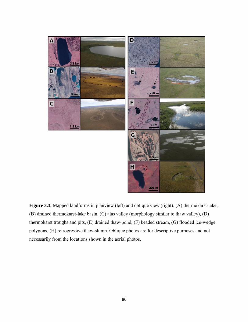
86
Figure 3.3. Mapped landforms in planview (left) and oblique view (right). (A) thermokarst-lake,
(B) drained thermokarst-lake basin, (C) alas valley (morphology similar to thaw valley), (D)
thermokarst troughs and pits, (E) drained thaw-pond, (F) beaded stream, (G) flooded ice-wedge
polygons, (H) retrogressive thaw-slump. Oblique photos are for descriptive purposes and not
necessarily from the locations shown in the aerial photos.

87
Figure 3.4. Mapped areas grouped by surficial geology. Letters correspond to those in Figure
3.1.

88
Figure 3.5. Distribution of thermokarst landforms in relation to surficial geology. The n values
indicate number of study areas underlain by each of the six surficial geology units. BS: beaded
stream, DTP: drained thaw pond, TV: thaw valley, RTS: retrogressive thaw slump.

89
Figure 3.6. Relationships between thermokarst, surficial geology, and the amount of ground ice
present. No estimates of ground ice are available for the glacial drift area.
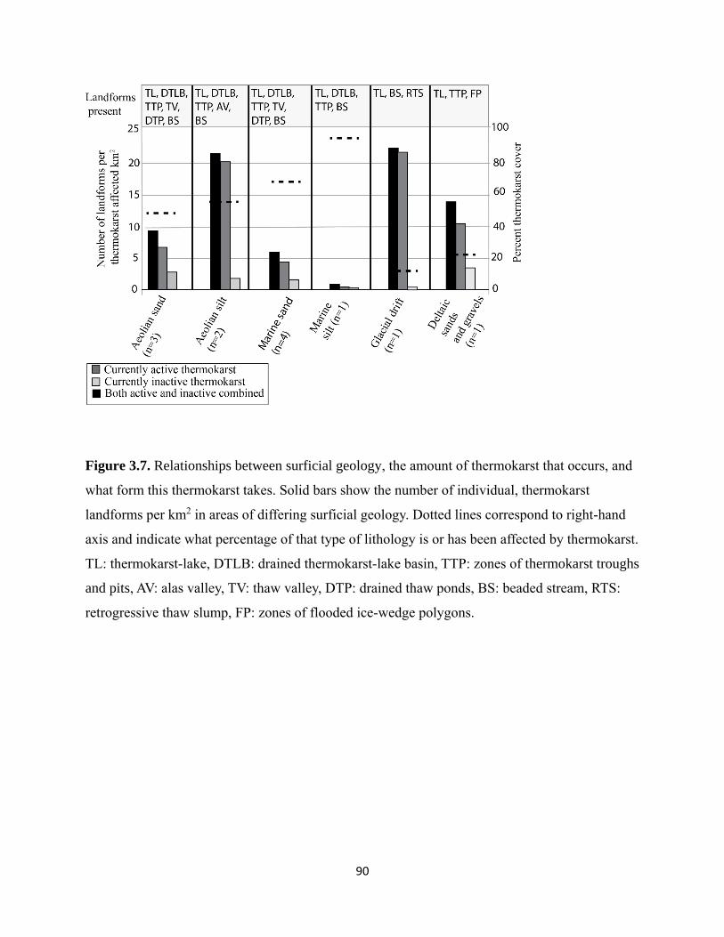
90
Figure 3.7. Relationships between surficial geology, the amount of thermokarst that occurs, and
what form this thermokarst takes. Solid bars show the number of individual, thermokarst
landforms per km2 in areas of differing surficial geology. Dotted lines correspond to right-hand
axis and indicate what percentage of that type of lithology is or has been affected by thermokarst.
TL: thermokarst-lake, DTLB: drained thermokarst-lake basin, TTP: zones of thermokarst troughs
and pits, AV: alas valley, TV: thaw valley, DTP: drained thaw ponds, BS: beaded stream, RTS:
retrogressive thaw slump, FP: zones of flooded ice-wedge polygons.

91
Figure 3.8. Number of drained thermokarst-lake generations observed (see example, top right) in
areas of differing surficial geology. Study areas L (glacial drift) and A (deltaic sands and gravels)
are not shown because no drained thermokarst-lake basins were mapped there.
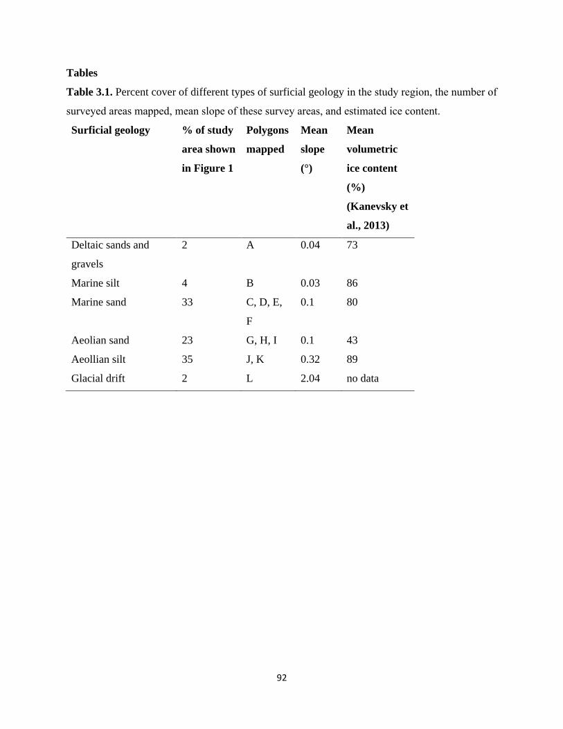
92
Tables
Table 3.1. Percent cover of different types of surficial geology in the study region, the number of
surveyed areas mapped, mean slope of these survey areas, and estimated ice content.
Surficial geology % of study
area shown
in Figure 1
Polygons
mapped
Mean
slope
(°)
Mean
volumetric
ice content
(%)
(Kanevsky et
al., 2013)
Deltaic sands and
gravels
2 A 0.04 73
Marine silt 4 B 0.03 86
Marine sand 33 C, D, E,
F
0.1 80
Aeolian sand 23 G, H, I 0.1 43
Aeollian silt 35 J, K 0.32 89
Glacial drift 2 L 2.04 no data
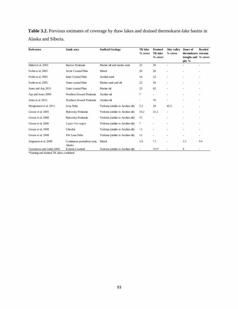
93
Table 3.2. Previous estimates of coverage by thaw lakes and drained thermokarst-lake basins in
Alaska and Siberia.
Alas valley
% cover
Hinkel et al. 2003 Barrow Peninsula Marine silt and marine sand 22 50 - - -
Frohn et al. 2005 Arctic Coastal Plain Mixed 20 26 - - -
Frohn et al. 2005 Inner Coastal Plain Aeolian sand 14 22 - - -
Frohn et al. 2005 Outer coastal Plain Marine sand and silt 22 45 - - -
Jones and Arp 2015 Outer coastal Plain Marine silt 23 62 - - -
Arp and Jones 2009 Northern Seward Peninsula Aeolian silt 7 - - - -
Jones et al. 2012 Northern Seward Peninsula Aeolian silt - 76 - - -
Morgenstern et al. 2011 Lena Delta Yedoma (similar to Aeolian silt) 5.2 20 42.5 - -
Grosse et al. 2005 Bykovsky Peninsula Yedoma (similar to Aeolian silt) 10.2 31.2 - - -
Grosse et al. 2008 Bykovsky Peninsula Yedoma (similar to Aeolian silt) 15 - - - -
Grosse et al. 2006 Laptev Sea region Yedoma (similar to Aeolian silt) 7 - - - -
Grosse et al. 2008 Cherskii Yedoma (similar to Aeolian silt) >1 - - - -
Grosse et al. 2008 SW Lena Delta Yedoma (similar to Aeolian silt) 13 - - - -
Jorgenson et al. 2008 Continuous permafrost zone,
Alaska
Mixed 1.9 7.1 - 2.3 0.4
Veremeeva and Gubin 2009 Kolyma Lowland Yedoma (similar to Aeolian silt) - 53.5* - 8 -
Zones of
thermokarst
troughs and
pits %
cover
Beaded
streams
% cover
*Existing and drained TK lakes combined
Reference Study area Surficial Geology TK lake
% cover
Drained
TK lake
% cover

94
Wh
ole
stu
dy
reg
ion
% C
ov
er
of
stu
dy
are
a
Wtd
%
Co
ve
r
reg
ion
% C
ov
er
of
stu
dy
are
a
Wtd
%
Co
ve
r
reg
ion
% C
ov
er
of
stu
dy
are
a
Wtd
%
Co
ve
r
reg
ion
% C
ov
er
of
stu
dy
are
a
Wtd
%
Co
ve
r
reg
ion
% C
ov
er
of
stu
dy
are
a
Wtd
%
Co
ve
r
reg
ion
% C
ov
er
of
stu
dy
are
a
Wtd
%
Co
ve
r
reg
ion
Wtd
%
Co
ve
r
TL
12.8
60.2
639.4
11.5
817.8
75.9
027.9
06.4
25.8
92.0
612.5
60.2
516.4
6
DT
LB
0.0
00.0
048.4
21.9
447.2
915.6
116.4
83.7
933.5
511.7
40.0
00.0
033.0
8
TT
P17.7
30.3
59.2
00.3
711.8
73.9
24.7
91.1
04.1
21.4
40.0
00.0
07.1
8
AV
/TV
0.0
00.0
00.0
00.0
02.7
50.9
10.9
30.2
114.0
34.9
10.0
00.0
06.0
3
DP
0.0
00.0
00.0
00.0
00.2
40.0
80.3
00.0
70.0
00.0
00.0
00.0
00.1
5
BS
0.0
00.0
00.1
60.0
11.0
20.3
40.3
30.0
80.4
70.1
60.7
90.0
20.6
0
FP
5.9
60.1
20.0
00.0
00.0
00.0
00.0
00.0
00.0
00.0
00.0
00.0
00.1
2
RT
S0.0
00.0
00.0
00.0
00.0
00.0
00.0
00.0
00.0
00.0
00.2
20.0
00.0
0
To
tal
tk
(%)
36.5
597.1
981.0
450.7
358.0
613.5
763.2
6
To
tal
no
tk
Co
ve
r(%
)
63.4
52.8
118.9
649.2
741.9
486.4
336.7
4
Gla
cia
l d
rift
De
ltaic
san
d a
nd
gra
ve
l
Ae
oli
an
san
dA
eo
lian
sil
tM
ari
ne
san
dM
ari
ne
sil
t
Tab
le 3
.3. P
erce
nt
cover
of
ther
mokar
st l
andfo
rms
acco
rdin
g t
o t
ype
of
surf
icia
l geo
logy;
wei
ghte
d p
erce
nta
ges
calc
ula
ted u
sing e
xte
nt
of
surf
icia
l geo
logy a
rea
show
n i
n F
ig. 1 a
nd d
escr
ibed
in s
ecti
on 2
, (T
L:
ther
mokar
st-l
ake,
DT
LB
: dra
ined
ther
mokar
st-l
ake
bas
in, T
TP
: zo
nes
of
ther
mo
kar
st t
roughs
and p
its,
AV
: al
as v
alle
y, T
V:
thaw
val
ley,
DP
: dra
ined
thaw
ponds,
BS
: bea
ded
str
eam
, F
P:
zones
of
flooded
ice
-wed
ge
poly
gons,
RT
S:
retr
ogre
ssiv
e
thaw
slu
mp)

95
Table 3.4. Spatial statistics for each type of landform across the entire study area and within
each type of surficial geology, (abbreviations as in Table 3)
Count Mean
elevatio
n range
(m)*
Mean
area (ha)
Min.
area (ha)
Max.
area (ha)
Range
(ha)
Std (ha)
Entire study area
TL 212 6.36 24.33 0.09 8.00 559.03 63.52
DTLB 168 6.93 61.69 0.02 864.32 864.31 108.29
TTP 887 - 3.14 0.00 230.04 230.04 14.17
AV/TV 88 8.97 11.89 0.00 77.65 77.64 14.03
DP 110 2.64 1.04 0.00 11.39 11.39 1.93
BS 37 10.67 4.80 0.08 26.53 26.45 6.37
RTS 2 2.77 1.37 4.18 2.81 1.99
FP 24 2.69 0.32 10.73 10.41 2.33
Total # 1528 (Currently active =1358, Currently inactive =170)
Deltaic sands and gravels
TL 35 4.74 8.08 1.17 105.30 104.13 17.87
DTLB 0 - 0.00 0.00 0.00 0.00 0.00
TTP 111 - 3.69 0.00 62.25 62.25 7.77
TV 0 - 0.00 0.00 0.00 0.00 0.00
DP 20 - 3.32 0.08 11.39 11.30 3.40
BS 0 - 0.00 0.00 0.00 0.00 0.00
FP 24 - 2.69 0.32 10.73 10.41 2.33
Total # 190 (Currently active=170, Currently inactive=20)
Marine silt
TL 9 3.53 109.92 1.51 559.12 557.61 188.23
DTLB 8 5.30 232.24 4.20 864.32 860.12 304.00
TTP 1 - 230.04 230.04 230.04 0.00 0.00
TV 0 - 0.00 0.00 0.00 0.00 0.00
DP 0 - 0.00 0.00 0.00 0.00 0.00
BS 1 2.51 4.69 4.69 4.69 0.00 0.00
Total # 19 (Currently active =11, Currently inactive=8)
Marine sand
TL 54 2.54 33.09 0.11 488.13 488.03 81.98
DTLB 72 5.01 58.89 0.29 635.03 634.74 101.52
TTP 266 - 4.50 0.00 181.03 181.03 15.34
TV 15 6.07 18.35 3.84 77.65 73.81 18.46
DP 55 1.67 0.36 0.00 4.10 4.10 0.56
BS 10 8.08 11.57 1.29 26.53 25.23 9.35
Total # 472 (Currently active=345, Currently inactive=127)
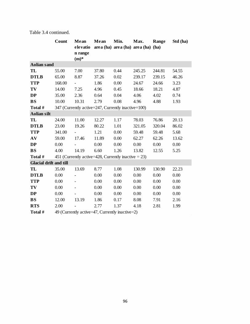
96
Table 3.4 continued.
Count Mean
elevatio
n range
(m)*
Mean
area (ha)
Min.
area (ha)
Max.
area (ha)
Range
(ha)
Std (ha)
Aolian sand
TL 55.00 7.00 37.80 0.44 245.25 244.81 54.55
DTLB 65.00 8.87 37.26 0.02 239.17 239.15 46.26
TTP 168.00 - 1.86 0.00 24.67 24.66 3.23
TV 14.00 7.25 4.96 0.45 18.66 18.21 4.87
DP 35.00 2.36 0.64 0.04 4.06 4.02 0.74
BS 10.00 10.31 2.79 0.08 4.96 4.88 1.93
Total # 347 (Currently active=247, Currently inactive=100)
Aolian silt
TL 24.00 11.00 12.27 1.17 78.03 76.86 20.13
DTLB 23.00 19.26 80.22 1.01 321.05 320.04 86.02
TTP 341.00 - 1.21 0.00 59.48 59.48 5.68
AV 59.00 17.46 11.89 0.00 62.27 62.26 13.62
DP 0.00 - 0.00 0.00 0.00 0.00 0.00
BS 4.00 14.19 6.60 1.26 13.82 12.55 5.25
Total # 451 (Currently active=428, Currently inactive = 23)
Glacial drift and till
TL 35.00 13.69 8.77 1.08 130.99 130.90 22.23
DTLB 0.00 - 0.00 0.00 0.00 0.00 0.00
TTP 0.00 - 0.00 0.00 0.00 0.00 0.00
TV 0.00 - 0.00 0.00 0.00 0.00 0.00
DP 0.00 - 0.00 0.00 0.00 0.00 0.00
BS 12.00 13.19 1.86 0.17 8.08 7.91 2.16
RTS 2.00 - 2.77 1.37 4.18 2.81 1.99
Total # 49 (Currently active=47, Currently inactive=2)
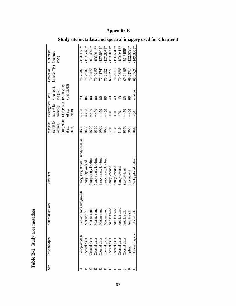
97
Appendix B
Study site metadata and spectral imagery used for Chapter 3
Site
Physi
ogra
phy
Surf
icia
l geolo
gy
Landfo
rmM
ass
ive
ice (
% b
y
volu
me)
(Jorg
enso
n
et
al.,
2008)
Segre
gate
d
ice (
% b
y
volu
me)
(Jorg
enso
n
et
al.,
2008)
Tota
l
volu
metr
ic
ice (
%)
(Kanevsk
iy
et
al., 2013)
Cente
r of
latitu
de (
°N)
Cente
r of
longitude
(°W
)
AF
loodpla
in d
elta
Deltaic
sands
and g
ravels
Peaty
, si
lty, fl
uvia
l +
sandy c
oast
al
10-3
0=
>50
73
70.7
646°
-154.4
776°
BC
oast
al pla
inM
ari
ne s
iltP
eaty
silt
y low
land
10-3
0=
>50
86
70.7
916°
-153.5
925°
CC
oast
al pla
inM
ari
ne s
and
Peaty
sandy low
land
10-3
0=
>50
80
70.2
055°
-151.4
040°
DC
oast
al pla
inM
ari
ne s
and
Peaty
sandy low
land
10-3
0=
>50
80
70.7
915°
-156.9
147°
EC
oast
al pla
inM
ari
ne s
and
Peaty
sandy low
land
10-3
0=
>50
80
70.6
474°
-157.8
963°
FC
oast
al pla
inM
ari
ne s
and
Peaty
sandy low
land
10-3
0=
>50
80
70.3
132°
-157.8
071°
GC
oast
al pla
inA
eolia
n s
and
Sandy low
land
5-1
0<
50
43
69.9
295°
-153.0
141°
HC
oast
al pla
inA
eolia
n s
and
Sandy low
land
5-1
0<
50
43
70.2
971°
-156.6
817°
IC
oast
al pla
inA
eolia
n s
and
Sandy low
land
5-1
0<
50
43
70.0
339°
-153.9
412°
JC
oast
al pla
inA
eolia
n s
iltS
ilty low
land
30-7
0=
>50
89
69.9
140°
156.6
158°
KU
pla
nd
Aeolia
n s
iltS
ilty u
pla
nd
30-7
0=
>50
89
69.3
271°
-152.0
796°
LG
lacia
ted u
pla
nd
Gla
cia
l dri
ftR
ocky g
lacia
l upla
nd
10-8
0<
50
no d
ata
68.9
769°
-149.8
352°
Tab
le B
-1. S
tudy a
rea
met
adat
a

98
Table B-2. Locations of permafrost boreholes used in this study.
Site Latitude N Longitude
Galbraith 68.479717° -149.488767°
Inigok 69.989617° -153.093833°
Umiat 69.395683° -152.142800°
Koluktak 69.751600° -154.617567°
Fish Creek 70.335233° -152.052000°
South Meade 70.628467° -156.835317°
Drew Point 70.864509° -153.906745°

99
Table B-3. Slope statistics for each surficial geology region calculated using the Scenarios
Network for Alaska (SNAP) 1km resolution Alaska slope model
(http://ckan.snap.uaf.edu/dataset/slope).
Mean Min Max Mean Min Max
Marine sand 0.10 0.00 1.24 0.06 0.01 0.12
Marine silt 0.03 0.00 0.11 0.04 0.02 0.06
Aeolian sand 0.10 0.00 0.71 0.06 0.01 0.14
Aeolian silt 0.32 0.00 1.80 0.27 0.05 0.70
Deltaic sands and gravels 0.04 0.00 0.21 0.01 0.00 0.02
Glacial drift 2.04 0.00 12.57 0.81 0.17 1.36
Regional slope (°) Mapped area slope (°)

100
Figure B-1. Study area A

101
Figure B-2. Study area B

102
Figure B-3. Study area C
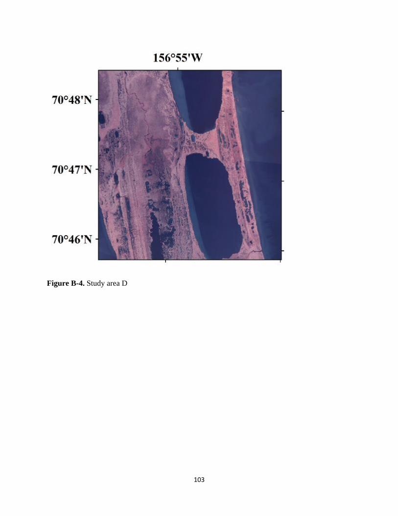
103
Figure B-4. Study area D

104
Figure B-5. Study area E
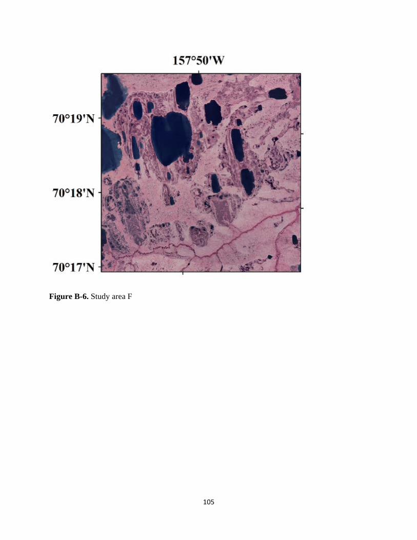
105
Figure B-6. Study area F
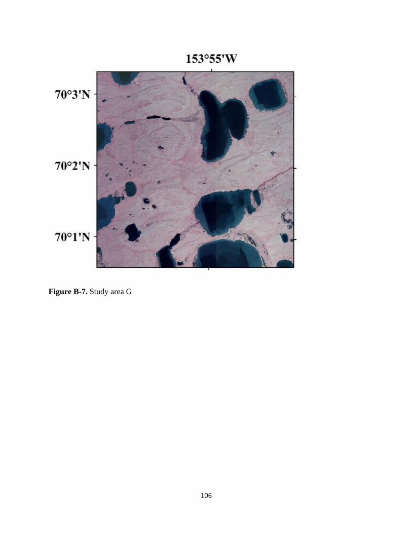
106
Figure B-7. Study area G

107
Figure B-8 Study area H

108
Figure B-9. Study area I
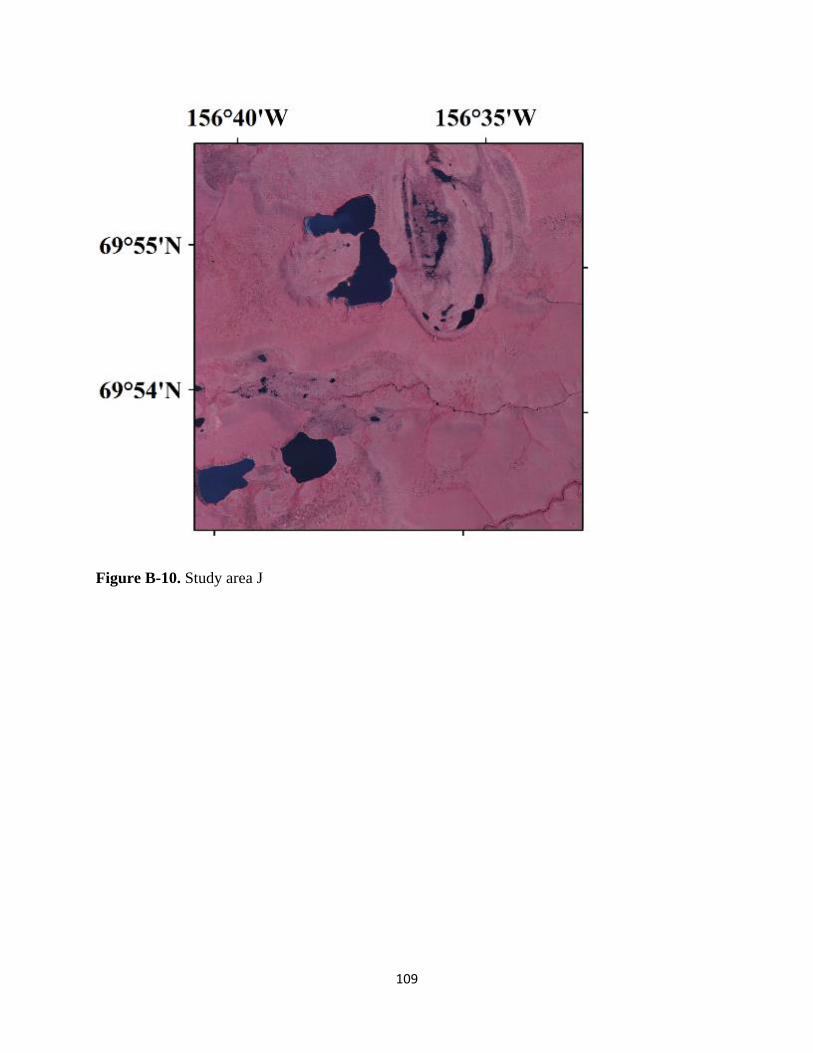
109
Figure B-10. Study area J

110
Figure B-11. Study area K

111
Figure B-12. Study area L

112

113
Chapter 4 High variability in shoreline response to declining sea ice in northwest Alaska3
4.1 Abstract
Climate is warming rapidly in the Arctic, and there is an urgent need to understand how
declining sea ice and thawing permafrost are affecting shoreline processes and coastal
geomorphology. Here, we explore the spatial and temporal patterns of shoreline change over the
past 64 years along two, geomorphologically distinct, storm-wave dominated reaches of the
Chukchi Sea coastline: a west- to southwest-facing, coarse-clastic shoreline (Cake Krusenstern
National Monument, CAKR) and a north-facing, sandy shoreline (Bering Land Bridge National
Park, BELA) both backed by permafrost bluffs. Using a combination of aerial and satellite
imagery, we map coastal changes during three time intervals: 1950-1980, 1980-2003, and 2003-
2014. We then explore this data in the context of changes in sea ice-free season. Results show
that between 1981 and 2014, sea ice duration in our study area has declined at 8 days per decade.
Changes in coastal geomorphology along both CAK R and BELA have been spatially variable
over the study period. Between 2003 and 2014, barrier island lowlands in BELA exhibited the
highest mean rates of change, -1.5 m-yr, while the foredunes in CAKR were the least dynamic as
no overall change was observed (mean rate of change, 0 m-yr). When compared to earlier time
intervals, the coastline of both BELA and CAKR have become much more dynamic between
2003 – 2004. Variability and range were highest in the most recent time interval for BELA and
CAKR. In CAKR, sample variance was 0.12, 0.16, and 0.26 m-yr, and in BELA 0.21, 0.10, and
0.53 m-yr for time intervals 1950 to 1980, 1980 to 2003, and 2003 to 2014 respectively. Overall,
mean erosion rates have been faster along BELA’s sandy coastline (overall max. -1.56 m-yr) than
in CAKR (overall max -0.3 m-yr); however, erosion rates in BELA have not responded linearly to
sea ice decline, probably because the frequency and magnitude of storms modifies the impact of
sea-ice decline on coastal erosion. We suggest that over the coming decades, the Alaskan
Chukchi coast will shift into a highly dynamic state before possibly settling into a new
geomorphologic equilibrium. Our results provide baseline data for a coastal region that could
3 Farquharson, L.M., Mann, D.H., Swanson, D.K., Jones, B.M., In Prep for Environmental
Research Letters, High variability in shoreline response to declining sea ice in northwest Alaska

114
experience radical changes over the next several decades, and provides policy makers with
helpful information required in assessing coastal community relocation in northwest Alaska.
4.2 Introduction
Arctic coastlines, (both bedrock and clastic coastlines located above 60°N, AMAP, 2012),
represent 34 % of the global total (Lantuit et al., 2012). Despite being protected by sea ice for 8
to 9 months of the year (Belchansky et al., 2004), some of these coastlines can be extremely
dynamic (Jones et al., 2009; Barnhart et al., 2014a). Warming climate and permafrost and
changes in sea ice cover (Lawrence and Slater 2005; Wang and Overland, 2009; Stocker et al.,
2014) threaten to trigger rapid and possibly drastic changes in coastal erosion and accretion
along Arctic coastlines over the coming century. Yet due to numerous non-linearities inherent to
the cryosphere (Miller et al., 2010; Serreze and Barry, 2011; Cohen et al., 2014), the future
geomorphological responses of Arctic coastlines to ongoing climate change remains poorly
constrained.
The combined presence of sea ice and permafrost endow Arctic coastlines with unique response
thresholds to climate change. Sea ice is a moderator of wave fetch and water temperature, and it
also shields coastlines from wave action, often for considerable portions of the year. The
duration of sea-ice cover in the Arctic has declined by ~13 % per decade since satellite
observations began in 1979 (www.nsidc.org), and over the last ca. 40 years the duration of land-
fast ice (seasonal ice frozen to the shoreface) has been declining by one week per decade
(Mahoney et al., 2014).The impact of sea ice decline has already been observed through an
increase in wave fetch, height and swell size in Arctic seas (Francis, et al., 2011; Overeem et al.,
2011; Thomson and Rogers, 2014; Thomson et al., 2016). The lengthening open-water season
has resulted in increasing wave energy available for coastal erosion and sediment transport
(Overeem et al., 2011). Another important effect of the changing sea-ice regime is the increased
probability that autumn storms will strike before the winter sea ice has re-formed (Forbes et al.,
2011). Storms occurring during the ice-free season generate the most geomorphologically
significant wave events along Arctic coastlines and hence strongly influence coastal processes
(Mason et al., 1996; Barnhart et al., 2014b).

115
The presence of permafrost introduces another set of unique processes to Arctic coastlines.
Rising air and water temperatures cause more rapid thaw of ice-rich permafrost along the coast.
In northern Alaska, long term permafrost monitoring sites show positive temperature trends of
0.21 °C and 0.66 °C decade−1 between 1995 and 2015 (Romanovsky et al., 2015), and mean
annual ground temperatures in the Bering Land Bridge National Park and Preserve are projected
to increase by up to 3 °C by 2050 (Panda et al., 2016). Warming is also evident offshore where
the sea surface temperature of the Chukchi Sea has risen by 0.5 °C per decade since1982
(Timmermans and Proshutinsky, 2015). Onshore, the potential impacts of permafrost thaw
include more rapid erosion of ice-rich bluffs, which in some regions is already extremely rapid
(Jones et al., 2009). Another possible effect is enhanced supply of sediment that could feed spit
growth and barrier island construction.
4.2.1 Previous studies
Previous studies of coastal dynamics along clastic, permafrost-affected shorelines include
research on the Beaufort Sea coast in Alaska (Hume and Schalk, 1967, Jorgenson and Brown,
2005; Mars and Houseknecht, 2007; Jones et al., 2009), the Beaufort Sea coastline of Canada
(Harper, 1990; Hequette and Barnes 1990; Solomon, 2005; Lantuit and Pollard, 2008;
Radosavljevic et al., 2016), and the Arctic-marginal seas of Siberia (Günther et al., 2013;
Günther et al., 2015).
Previous Arctic coastal research has focused on the often spectacular erosion of ice-rich
permafrost bluffs (including, but not exclusively, McCarthy, 1953; Jones et al., 2009; Gunther et
al., 2015;), and to a lesser extent on the dynamics of Arctic barrier-island systems (Harper, 1990;
Hequette and Ruz, 1991; Gorokhovich and Leiserowitz, 2011). Few studies (Hequette and Ruz,
1991; Radoslavic et al., 2016) have explored how permafrost-affected Arctic coastlines of mixed
morphology and grain size respond to sea-ice decline and permafrost thaw.
Previous work in the region of focus for this paper have explored rates of coastal change between
1950 and 1980 and used instantaneous water line as a proxy for the coast (Manley et al., 2007a).
Mean rates of change for the region showed an overall erosion trend between 1950 and 1980, but
an overall accretion trend between 1980 and 2003 (Gorokhovich and Leiserowiz, 2011). Within

116
the Arctic Coastal Dynamics database, the coastline of northwest Alaska is classified as “stable
or aggrading” (Lantuit et al., 2012).
Here we use repeat aerial and satellite imagery to estimate rates of coastal change on two
geologically distinct, coastal systems between 1950 and 2014 along 420 km of coastline in the
southwestern Chukchi Sea. Specifically, we address these questions: 1) How have coastal
dynamics varied over the last 64 years? 2) How variable is erosion and deposition in areas of
differing coastal geomorphology? 3) What is the relationship between sea-ice decline and rate of
coastal change?
4.3 Study area: Climate, weather, and sea ice
The coastlines of BELA and CAKR are located between ~65 and 67 °N and are bounded by
Kotzebue Sound and the southern Chukchi Sea (Figure 4.1). The modern day coast was
established between 5000 and 3000 years BP when eustatic sea level stabilized after
transgressing across the former Bering Land Bridge (Mason et al., 1995), while some features
including the barrier islands in SW BELA formed as recently as 17 ka (Jordan and Mason,
1999). The region is situated within a zone of continuous permafrost and has a mean July air
temperature of 13°C, a mean annual temperature of -5°C, and a mean precipitation of 25 cm
(NCDC 1981-2010 monthly normals for Kotzebue, http://www.wrcc.dri.edu/). Prevailing winds
blow from the west, north or north west (LaBelle et al., 1982). The Chukchi Sea is micro-tidal
(<1 m).
Sea ice in the southern Chukchi Sea typically forms in mid-November and persists until mid-
June, leaving on average five months of open water. Landfast ice, sea ice frozen to the shoreline,
expands outward from the shore starting in October and eventually extends up to 10 km offshore
in CAKR and 50 km in BELA. Landfast ice then retreats rapidly in May and June (Mahoney et
al., 2014).
The coastline of the Chukchi sea is characterized by a storm wave climate, and storm related
waves are considered a critical control over coastal processes (Jordan and Mason, 1999; Stutz
and Pilkey, 2001). Extratropical cyclonic storms typically track northwards into the Chukchi Sea
from the northeastern Pacific (Mason et al., 1996). Storms also arrive from the Arctic Ocean to
the north in the form of polar lows (Rasmussen et al., 2004). Storm intensity is greatest in the
autumn and winter (Mason wt. al., 1996) when low-pressure systems can raise sea level by 2-7

117
meters (Hume and Schalk 1967), and wave heights can reach up to 10 m or more
(https://www.ncdc.noaa.gov/stormevents/). Shallow water depths of 20 m or less extend 15 – 25
km offshore and contribute to the intensification of the resultant storm surges.
A combination of different sediment sources and ocean currents has resulted in very different
grain size compositions and shoreline morphology between CAKR and BELA. CAKR receives
coarse sands and gravels from the Baldwin Peninsula, a large mid-Pleistocene, terminal moraine
that forms much of the eastern shoreline of Kotzebue Sound (Huston et al., 1990). Strong anti-
clockwise current transport this material exclusively NW to the coast of CAKR (Panteleev et al.,
2013). In contrast, BELA receives only fine grained material, from Pleistocene aeolian deposits
located offshore, the Yukon Delta (Nelson and Creager 1977), and local yedoma and thaw lake
deposits which blanket the coastal lowlands of the northern Seward Peninsula (Jones et al., 2011;
Farquharson et al., 2016; Lenz et al., 2016).
BELA and CAKR are geomorphologically diverse and consist of a mixture of barrier island
systems, spits, foredune plains, and ice-rich permafrost bluffs (Figure 4.2). As such, they provide
an excellent opportunity to explore how diverse Arctic coastlines respond to similar changes in
sea-ice regime and temperature.
4.3.1 Bering Land Bridge National Park and Preserve (BELA)
The sand-dominated BELA coastline is located on the northern Seward Peninsula and is
composed of two reaches, one facing north and northwest into the southern Chukchi Sea, and the
other facing east into Kotzebue Sound (Figure 4.1.). Along the northwest-facing shoreline, wave
fetch is limitless during the ice- free season (Figure 4.1 inset). In contrast, within Kotzebue
Sound the fetch reaches a maximum of 95 km. Offshore bathymetry is shallow and gently
sloping, and the 20 meter isobath occurs between 10 and 50 km offshore, deepening to a
maximum of 55 m in the Bering Strait, approximately 160 km to the west. The relatively warm,
Alaska Coastal Water current carries Bering Sea water northward through Bering Strait into the
Chukchi Sea seaward of the -20 meter isobath (Mason et al., 1997; Grebmeier 2012).
Along the coast of BELA, the seasonal timing of coastal processes are limited by the open-water
season (here defined as <30 % sea ice cover in the nearshore zone). The open-water period
currently begins in the first week of June and usually ends (>30 % sea ice cover) in the third

118
week of November (averages based on sea ice data 1982–2015, Figure 4.3.). During the open
water season, coastal dynamics are driven by a combination of micro- tidal and wave-dominated
processes as well as by the thermo-abrasion and thermo-denudation of ice-rich, permafrost
bluffs. Thermo-abrasion is the erosion of permafrost coasts by a combination of thermal and
mechanical action by ocean waves while thermo-denudation is the erosion of permafrost through
the combined power of solar radiation and gravity (Are, 1988). Despite a micro-tidal regime,
storms can create surges up to 4 meters high, often overwhelming the tidal signal (Wise et al.,
1981). The resulting coastal geomorphology is a complex mixture of barrier lagoon systems, ice-
rich permafrost bluffs, aggrading spits, and estuaries (Figure 4.3). Shallow nearshore bathymetry
allows for the formation of offshore sand bars, 0.5-3 km wide, which are most prominent at the
eastern tip of Cape Espenberg and to the south in Kotzebue Sound.
The north-facing shoreline of BELA contains three large lagoon systems, which reach over 400
km2 in size and are separated from the sea by low-lying barrier islands ranging from 7 to 50 km
in length. These barrier islands are characterized by wide and gently sloping sandy shorefaces
that act to dissipate wave energy. Lagoon backshores are formed by ice-rich, permafrost bluffs
dissected by numerous streams. Salt marshes are widespread in back-barrier areas, existing only
ca. 0.5 m above sea level. Washover channels, relict foredunes, and capes provide evidence of
past storm events and shifts in the locations of tidal inlets (Mason et al., 1997; Jordan and
Mason, 1999). Inland of the coast is a broad tundra lowland dotted with thermokarst lakes,
drained thermokarst lake basins (Jones et al., 2011, Farquharson et al., 2016; Lenz et al., 2016),
and ice-rich loess (yedoma) (Figure 4.3b). These deposits accumulated in synchrony with
massive syngenetic ice wedges during the mid- to late Pleistocene and have subsequently been
reworked by thermokarst during the Holocene (Farquharson et al., 2016; Lenz et al., 2016).
4.3.2 Cape Krusenstern National Monument (CAKR)
The gravel-dominated Cape Krusenstern National Monument contains two coastal reaches, one
facing west and the other southwest (Figure 4.1). The fetch on the west-facing coastline can be
up to ~500 km during the open water season. The fetch on the southwest-facing shoreline is less,
reaching a maximum fetch of 95 km. Offshore, bathymetry is characterized by a slightly steeper
gradient than at BELA (Figure 4.1).

119
The coastal geomorphology of CAKR differs to BELA by being characterized by narrow,
moderately sloping gravel beaches, narrow gravel bars, high permafrost bluffs with only a
moderate ground ice content, and an extensive coarse-clastic beach-ridge plain (Figure 4.3). The
lagoons remain isolated from the sea except in spring when ephemeral channels form briefly
during break up and dissect lagoon gravel bars. The backshore of lagoons are characterized by
sloping, vegetated permafrost bluffs drained by water tracks and small streams. Most lagoons are
fronted by a gravel barrier consisting of an overwash terrace standing ~ 1 m above the supratidal
zone of the outer beach and covered by rye grass (Leymus mollis). Cape Krusenstern Lagoon
forms an exception and is characterized by a convex sweeping shoreline formed from the
systematic progradation of numerous beach ridge sets (Mason and Jordan, 1993).
4.4 Methods
We assessed coastal change along 480 km of shoreline, including 340 km in BELA and 140 km
in CAKR, using ortho-rectified aerial imagery from 1950, 1980, and 2003 (Manley et al., 2007b,
c, d). For the 2014 period, we acquired both panchromatic and multispectral WorldView-2
satellite imagery that was ortho-rectified using a 2012 IfSAR derived digital surface model and
further georeferenced to the 2003 aerial images of Manley 2007d following the standard
operating procedures of Manley and Lestak (2012).
4.4.1 Shoreline digitization and measuring change
To estimate shoreline changes, we mapped the erosion scarp (ES) where it was visible. The ES
was defined as a topographic break between the permafrost bluff or foredune and the beach
(Boak and Turner, 2005). This feature was chosen because it was visible across all time periods,
was present along significant portions of the coastline, and is directly related to erosional
processes. The main issue with this and a majority of non-datum related proxies is that it
primarily indicates where erosion is occurring, and rarely allows for measurement of deposition
(Boak and Turner, 2005). If an erosion scarp was not present, we mapped the seaward vegetation
line, which was identified by abrupt spectral differences between the vegetation and the beach
(Boak and Turner, 2005).
120
Once the shoreline was mapped for all time periods (1950, 1980, 2003, 2014), we calculated
rates of shoreline change using the U.S. Geological Survey Digital Shoreline Analysis Tool
(DSAS) (Thieler et al., 2009) at 50 m increments along the 420 km of shoreline for each time
step. Measurements were only possible where the ES was consistently present between time
periods. In some cases, notably in the cases of interdune areas and salt flats, the ES was present
only intermittently.
Error estimates for erosion rates were calculated using the following equation:
where Ep1 and Ep2 represent the pixel resolution of the imagery for each year, RMS1 and RMS2
are the root mean square errors from georegistration of an image for each year, and ∆t is the time
interval associated with a given time step. Errors for each time slice can be found in Table 4.1.
To explore the drivers of coastal dynamics, we compared coastal dynamics between BELA
(sand-dominated) and CAKR (gravel-dominated) and also classified the shoreline according to
supratidal-zone geomorphology (Table 2). Coastal geomorphology classes included: beach ridge,
foredune, barrier interdune, welded barrier, and permafrost bluff.
4.1.2 Ground-truthing
To check the accuracy of our digital mapping efforts, we conducted field surveys during the
summer of 2015 on foot along 40 km of coastline (20 km in each of CAKR and BELA), as well
as low-elevation aircraft flights along 150 km and 60 km in BELA and CAKR, respectively.
While mapping, we frequently referred to the oblique coast photographs provided by the Alaska
Shorezone Coastal Mapping and Imagery tool (NOAA
https://alaskafisheries.noaa.gov/mapping/szflex/). We also utilized the long- term shoreline
surveys conducted by Jordan et al. (pers comm.) and conducted additional measurements at five
of his sites (three in BELA and two in CAKR) during the summer of 2015 (Figure 4.1). To
ground-truth our remote-sensing based estimates of erosion rates, we repeatedly measured from
two permanently installed survey markers to the edge of the permafrost bluff or foredune.

121
We found that our field measurements closely aligned with our remote sensing efforts (R2=0.74)
with a maximum offset of only 0.12 m yr-1
4.1.3 Sea ice data
Sea ice concentrations for the period 1982 to present were calculated for two representative areas
of 25 km2 located offshore of the two study areas (Figure 4.1) and percent sea ice cover was
analyzed at a weekly resolution. Estimates of sea-ice concentration were from a combination of
Special Sensor Microwave Imager (SSM/I) data (Comiso and Nishio 2008) and Advanced Very
High Resolution Radiometer (AVHRR) radiometric surface temperature between 1982 and 2008
(Figure 4.3). A sea ice concentration of 30 % was selected for the threshold between open and
closed water.
4.5 Results
4.5.1 Open water season and storm events
Analysis of trends in sea ice for near shore sections of our study area show that the open water
season is extending at ~ 8 days per decade (Figure 4.3). Between 1981 and 2014 sea ice breakup
is occurring approximately two weeks earlier and sea ice formation is occurring approximately
two weeks later. Sea ice decline trends are similar for both coastlines, with BELA exhibiting a
slightly greater increase than CAKR by less than a day per decade. Despite a negative trend in
sea ice extent between 1981 and 2014, sea ice extent fluctuates from year to year between shorter
and longer ice free seasons. In general, we observed that years which exhibited a longer ice free
season were characterized by both early break up in spring and late formation in fall. For years
which exhibited a shorter ice free season, the opposite held true.
4.5.2 Spatial and temporal patterns of shoreline change in the Chukchi
Rates of coastal change were variable across both the two study areas and the different time
periods. In BELA, mean rates of change were -0.68 m yr-1, -0.26 m yr-1 and -0.68 m yr-1 for T1,
T2, and T3 respectively. In CAKR, mean rates of change were -0.04 (stable when errors are

122
taken into account), -0.22 m yr-1, and -0.13 m yr-1 for T1, T2, and T3 respectively. Overall BELA
exhibited the highest rates of change and was found to be the more dynamic coastline.
In both BELA and CAKR, the most recent study period, T3, is characterized by the highest
variance (s2) in rates of change (Table 4.3). In BELA s2= 0.21, 0.10, and 0.53 and in CAKR,
s2=0.12, 0.16 and 0.26 for T1, T2, and T3, respectively (Table 4.3). Similarly, the highest range
of rates-of-change values occurred in recent years along both shorelines. In BELA, the rates of
change in each survey interval were 2.59, 2.01 and 4.79; while in CAKR they were 3.34, 3.83,
and 6.54. A possibly confounding factor in these variance estimates is the difference in study
period length (30 yr, 24 yr, and 11 yrs) (Dolan et al., 1991). To explore this relationship, we
plotted sample variance against length of time period for T1, T2, T3 using only transect points
that had values for all three time periods (n=922). We found that there was a weak negative
correlation (r2=0.34, Appendix C), suggesting that high sample variance in T3 is a real
phenomenon and not a manifestation of statistical analysis.
Changes in the rate of shoreline change differed in BELA and CAKR over the three observation
periods (Figures 4.4, 4.5, 4.6, 4.7). Mean rates of change in BELA were highest for T1 and T3, at
-0.68 m yr-1 for both time periods. CAKR exhibited slower erosion rates, and interestingly
showed the highest mean rate of change during T2 at -0.22 m yr-1, compared to -0.04 m yr-1 for
T1, and -0.13 m yr-1 for T2 (Table 4.3).
In BELA, the rate of change has become increasingly negative between T2 and T3 (∆T2/3),
compared to a positive shift between T1 and T2 (∆T1/2) (Figures 4.8a, 4.b). An increasing
number of transects are beginning to switch either from stable to erosional, or accretionary to
erosional for ∆T2/3. Overall, this data suggests that changes in the rate of erosion are out pacing
changes in the rate of accretion (Figure 4.8a, b).
In contrast, CAKR rates maintained a similar distribution between T1 and T2 (∆T1/2), and
between T2 and T3 (∆T2/3). During these intervals, changes were equally distributed between
erosion and accretion (Figures 4.8c, d). Most transects that initially were stable or accreting
during T2 later shifted towards negative rates. ∆T2/3 exhibited a wider range of rate changes
compared to ∆T1/2, suggesting an overall increase in coastal dynamism in CAKR during our
study period (Figure 4.8c, d).

123
4.5.3 What type of shorelines eroded most rapidly?
Erosion rates varied alongshore and between different coastal geomorphology types. Within
BELA, a clear erosion gradient exists that reflects longshore drift. Along the north-facing
barrier-lagoon system (Figure 4.1), longshore drift is driving rapid erosion (up to -5 m yr-1) in the
southwestern area along with barrier island migration (Figure 4.4), while at the same time
accretion has occurred to the northeast on the Cape Espenberg spit (Figure 4.5). This pattern has
been accentuated over time, with T3 exhibiting the strongest along-shore gradient in erosion
rates.
Within BELA, shorelines associated with barrier islands have experienced the most dramatic
changes with mean rates of erosion up to -1.53 m yr-1 between 2003 and 2014 in low-lying areas
between foredunes. Through T1, T2, and T3, mean rates of shoreline change along low-lying
interdune areas were -0.82 m yr-1, -0.59 m yr-1, and -1.53 m yr-1, respectively (Table 4.3). The
foredunes themselves changed at slightly slower rates: -0.86 m yr-1, 0.34 m yr-1, and 0.93 myr-1
for T1, T2 and T3, respectively (Table 3). Interestingly, foredunes along the BELA coast
exhibited the maximum rates of erosion observed anywhere in the study, -4.79 m yr-1 during T3.
In contrast, ice-rich permafrost bluff s eroded more slowly, with a maximum retreat rate of 0.51
myr-1 between 1950 and 1980. Through T1, T2, and T3, mean rates of erosion along permafrost
bluffs were -0.51 m yr-1, -0.18 m yr-1, and -0.32 myr-1, respectively.
Compared to BELA, In CAKR, the spatial distribution of erosion rates was more complex than
in BELA. Sediment deposition and shoreline progradation was focused primarily at Cape
Krusenstern lagoon, which is located at the entrance to Kotzebue Sound. Along this part of the
coastline, both erosion and accretion were most rapid during T3, and slower during both T1 and
T2. Overall, permafrost bluffs exhibited the highest mean erosion rates at CAKR (-0.16, -0.30
and -0.20 for T1, T2, and T3 respectably), yet the maximum rates of erosion (-3.57 myr-1) were
observed along welded gravel barriers (Figure 4.2d), adjacent to tidal inlets during T3.
No clear, along-shore gradient in erosion/accretion rates exists in CAKR. The most dynamic
parts of this coastline are in Cape Krusenstern Lagoon were on the southeast-facing beach

124
ridge/lagoon complex at the mouth of Kotzebue Sound, where frequent alternations between
erosion and accretion occurred.
4.5.4 Erosion processes
Several different erosion processes occur, some of which are unique to particular types of
coastline (Figure 4.9). Erosion along permafrost bluffs appeared to be primarily due to thermo-
erosion and thermo-denudation, although there is a marked absence of the thermo-abrasion niche
cutting and block collapse observed along the Beaufort Coast (Barnhart et al., 2014).
Thermoerosion gullies developed in permafrost bluffs backing the BELA coastline between 2003
and 2014, which contributed to the erosion of these bluffs. Coastal erosion along the barrier
islands consisted of three main processes: along foredunes, i) dune front undercutting and
collapse, and along inter-dune areas, ii) the formation of overwash capes, probably during
storms, and ii) aeolian sediment transport inland across the barrier island.
4.5.5 Accretion – location and process
Accretion within BELA was confined to the Cape Espenberg spit. Although the absence of
wave-modified vegetation lines made it difficult to precisely map accretion along the spit, the
imagery series revealed progressive welding of offshore sand beach ridges onto the shoreface
(Figure 4.2d).
Accretion within CAKR was more widespread and obvious. Along welded barriers and in front
of the beach ridges adjacent to Cape Krusenstern Lagoon, seaward movement of the vegetation
line clearly revealed beach accretion. During the T3 interval, maximum rates of accretion were
1.3 and 3 myr-1 along the welded barriers and the beach ridges adjacent to Cape Krusenstern
Lagoon, respectively. While the temporal resolution of the imagery does not reveal the exact
process responsible, the most likely one involves sand and gravel being deposited along the
seaward margin of the supratidal zone upper sections of the beach, which is then colonized by
vegetation.

125
4.6 Discussion
4.6.1 How have coastal dynamics in the Chukchi Sea varied over the last 64 years?
The coastlines of NW Alaska have become more dynamic during 2003 – 2014 compared to the
previous 53 years. We attribute this trend in part to an increase of ~ 0.8 days/yr for the open
water season and corresponding impacts on wave-climate.
Results from this study indicate a high amount of variability in coastal change between different
coastal morphologies. In general, we found the gravelly coast of CAKR to be much less dynamic
with a more muted increase in sample variance and mean rates of change compared to the sandy
coast of BELA. Despite these clear differences, coastal processes are becoming more vigorous in
both BELA and CAKR. Along both coastlines during T3, we observed the greatest range and
variability in rates of change suggesting that both erosion and accretion are ramping up, leading
to a more dynamic coastline.
Despite a relatively linear decline in sea ice duration over the study period, both coastlines
showed nonlinearities in their response. In BELA erosion rates and rate variance were high
between 1950 and 1980, slowed between 1980 and 2003, and ramped up to the most dynamic
state observed during the most recent observation period, 2003 - 2014. In contrast, CAKR
experiences the highest rates of change during T2, but a stepwise increase in variance through
the three observation periods.
Sections of coastlines with contrasting geomorphology exhibited quite different rates of change.
In both BELA and CAKR, ice-poor beach ridge, foredune and interdune areas were the most
dynamic. Rates of erosion along ice-rich permafrost bluffs in BELA were slow compared to
other types of coastal geomorphology. Locations of rapid change along permafrost bluff sections
were often associated with the formation of small retrogressive thaw slumps which are episodic
in their formation and retreat, a phenomena also observed on the eastern Beaufort (Obu et al.,
2016).
An increase in coastal dynamics has also been observed along the Beaufort Sea Coast, along both
ice-rich permafrost bluffs (Jones et al., 2009) and clastic coastlines of mixed morphology in the
western Beaufort (Radoslavic et al., 2016). Observations in the Canadian Beaufort Sea coast
show a similar non-linear response to sea ice decline (Radoslavic et al., 2016). In contrast, ice-

126
rich permafrost bluffs along the western Beaufort Sea coast experienced a step-wise increase in
erosion rates between 1955 and 2007 (Jones et al., 2009). At lower latitudes, along the Atlantic
seaboard a combination of changing wave-climate, sea level rise, and an increase in the
frequency of intense storm events is projected to cause erosion and accretion to speed up and
cause large-scale changes in shoreline morphology (Slott et al., 2006).
The rates of change we observe in BELA and CAKR are slower than those observed on the
Beaufort Coast and in Siberia. Observations along the Tuktoyuktuk Peninsula note the rapid
landward migration of barrier systems at up to ~ 3myr-1 (1950 – 1980, Hequette and Ruz, 1991).
Mean erosion rates of ice rich permafrost bluffs along the Beaufort for the period 2002 to 2007
were 13.6 m yr-1 (Jones et al., 2009) and in Siberia averaged -3.4 +/- 2.7 m yr-1 between 2010 and
2013 (Gunther et al., 2015). This variation is likely due to several factors, including height of the
backshore as suggested to Lantuit et al. (2012) and the processes controlling erosion (denudation
vs. abrasion and block collapse) (Jones et al., 2009).
4.6.2 Causation
At a regional level the coastlines of BELA and CAKR appear to be responding to climate change
related environmental forcing. Sea ice is declining in our study area (Figure 4.3), making more
energy available for amplification of coastal processes. Nonlinearities apparent in mean rates of
change and sample variance are probably due to the influence of other key environmental
factors, primarily storm direction, frequency, and magnitude (Mason et al., 1997).
At a more local level, we suggest that beach morphology, grain size and shoreline aspect
contribute to the wide range in coastal dynamics in our study area. CAKR’s coarse-grained
shoreline is characterized by steeper beaches (6°) compared to BELA (3-4°). As such, more
wave energy is reflected from the CAKR shoreline, while at BELA wave energy is dissipated
across the shoreface (Masselink and Short, 1993; Cowell and Thom, 1994). Waves breaking at
CAKR cannot propagate as far inland and as such are less likely to cause erosion of landforms
along the backshore. Fetch and shoreline orientation also influence how wave energy interacts
with the shore with maximum longshore transport occurring when waves hit the shoreline at
angles of ~40 - 50 ° (Anderson and Anderson 2010; Pye and Blott, 2008). Storms mainly arrive
from the Arctic Ocean to the north, or the Bering Strait to the southeast. BELA’s NW facing

127
orientation and open fetch may result in different patterns of wave energy dissipation compared
to CAKR.
4.6.3 How will the Chukchi Sea coast change in the future?
Making predictions of coastal change is challenging, due to the non-linear nature of so many
coastal sedimentary processes (Fitzgerald et al., 2008; Carrasco et al., 2015). The presence of
ice-related processes possessing striking thresholds inherent in their phase-change physics make
it even harder to predict changes along Arctic coastlines, especially when climate is changing
rapidly. On the coast of the Chukchi Sea, five factors may strongly influence coastal dynamics
over coming decades (Figure 4.10): warming permafrost, air, and ocean temperatures; attendant
sea-ice decline; sea level rise; shifts in the frequency and tracks of storms; and changes in the
wave regime related to all the above factors.
Geomorphic systems tend to recover from high magnitude disturbance event such as storms by
relaxing back to their prior state. For instance, a shoreface over-steepened during a high-wave
event will prograde seaward to reestablish its pre-storm profile. However, if the frequency or
intensity of disturbances becomes faster and/or greater than the recovery phase, the system may
be propelled to a new quasi-stable state. In this case, rising RSL and warming temperature may
increase the frequency of storm-wave events and thermokarst (Figure 4.10).
As the open water season continues to extend, the coastlines of BELA and CAKR will become
more dynamic. Areas already characterized by erosion will see rates increase, while areas of
sediment deposition will accrete more rapidly. This pattern is evidenced in Holocene records of
shoreline change in BELA, whereby periods of increased storminess caused the formation of
transgressive dune bodies offshore which migrated landward, eventually becoming welded to the
Cape Espenberg (Mason et al., 1995)
One potential major geomorphological threshold in BELA may be the destruction of barrier
islands in the SW sector of the coastline. This section of coast is already experiencing the
quarrying of sediments due to long-shore drift (Jordan and Mason, 1999). An increase in sea
level will also contribute to more barrier overwash events, where beach material is transported
landward (Jordan and Mason, 1999). Barrier island morphology may be stressed even further if
the storm climate ramps up and leads to an increase in overwash events and the formation of
128
inlets (Fitzgerald et al., 2008). If barrier islands in BELA do disappear this would expose ca. 100
km of ice-rich permafrost bluffs currently protected by barrier systems to open water and more
aggressive erosion.
Ice-rich permafrost bluffs may be subject to another threshold effect. Shoreline retreat in the face
of rising RSL or increased wave attack is accompanied by re-equilibration of the entire shoreface
profile, and in many cases this involves sediment being transferred offshore from the former
supratidal zone offshore. In cases where the shoreline contains ice-rich permafrost, a slight rise
in RSL or wave energy can push the shoreline far out of equilibrium because instead of
sediment, the former shoreline was ice. To reestablish the equilibrium profile, the shoreline must
retreat still further inland to acquire sufficient sediment. This type of dynamic probably underlies
the ongoing retreat of ice-rich bluffs along the Beaufort Sea where erosion rates exceed 13 m yr-1
(Jones et al., 2009). In our study area, we suspect the coastal reaches in BELA where ice-rich
yedoma bluffs occur are vulnerable to this kind of “threshold-accentuated Bruun retreat” (Bruun,
1962) involving extremely rapid coastal retreat. At present permafrost bluffs in both BELA and
CAKR are largely protected by wide beaches. If sea level rises and mean high tide reaches the
base of bluffs, this may convert our study coastlines from being dominated by thermodenudation
to being dominated by thermoabrasion, notch formation, and bluff collapse as seen on the
Beaufort Coast (Jones et al., 2009).
The way in which eroded material is redistributed is a critical component in the future response
of BELA and CAKR. While normal weather conditions are likely to continue facilitating
longshore drift and a fair amount of sediment deposition onshore, while storms drive erosion and
result in net offshore transport (Mason et al., 1997). The composition of landforms being eroded
is also an important factor. Sandy sediment eroded from foredunes could remain within the on
and near shore sediment budget, supplying material for beach nourishment. One potential
outcome of this is the growth of transgressional dunes along Cape Espenberg Spit (Jordan and
Mason 1999). Conversely, more frequent and intense storms could result in periods of aggressive
erosion and barrier overwash, and may result in an increase in sediment transport offshore. Loess
eroded from ice-rich permafrost bluffs will likely be transported offshore in suspension.

129
4.7 Conclusions
The results of this study explore sea ice decline and rates of coastal change along a 450-km
stretch of coastline in the Chukchi Sea. The sea ice season in this region has decreased at ~ 1
day/yr since satellite observations began, which has inevitably lead to an increase in the amount
of energy available for sediment transport. We find that coastal geomorphology is responding to
ongoing climate change by becoming more dynamic in the form of increased erosion and
accretion. This increased dynamism varies markedly between different stretches of coastline and
between the coastal landforms which make up each. Low lying sections of barrier island
characterized by salt marshes and interdunes in BELA were the most dynamic, and were found
to erode at a mean rate of -1.53 m yr-1 for the period 2003 - 2014. In contrast, foredune
complexes in CAKR were found to be the most stable. Interestingly we observed that rates of
erosion along ice-rich permafrost bluffs were quite slow, -0.3 m yr-1 for 2003-2014 when
compared to other regions.
The results of this chapter demonstrate that coastal response to climate change is complicated
and non-linear. Despite a recent increase in dynamism being observed in both BELA and CAKR,
we found that the three time slices studied did not necessarily exhibit a step wise increase in
mean rates of change, range of rates, or sample variance. We attribute this nonlinear response to
negative feedback loops within the coastal system.
Of particular concern is the possibility that a geomorphic threshold may exist in the study
region’s shorelines, perhaps involving the onset of rapid, thermo-abrasion similar to coastal
erosion of ice-rich bluffs along the Beaufort Sea coast. If the frequency of disturbance events
increases, this may lead to barrier island decay, exposure of ice-rich permafrost bluffs, an
increase in the rate of permafrost degradation, and more sediment deposition along Cape
Espenberg Spit and Cape Krusenstern Lagoon.
Acknowledgements
This study was funded by a National Park Service cooperative agreement with the University of
Alaska Fairbanks. We thank China Kantner and Sara Grocott for field assistance. We thank Uma
Bhatt for providing sea ice data and James Jordan for providing unpublished data on coastal
surveys for the study area.

130
4.8 References
AMAP, 2012. Arctic Climate Issues 2011: Changes in Arctic Snow, Water, Ice and Permafrost.
SWIPA 2011 Overview Report.
Anderson, R.S. and Anderson, S.P., 2010. Geomorphology: the mechanics and chemistry of
landscapes. Cambridge University Press.
Are´ F.E. 1988. Thermal abrasion of sea coast. Polar Geography and Geology 12. Silver Spring,
MD: V.H. Winston.
Barnhart, K.R., Anderson, R.S., Overeem, I., Wobus, C., Clow, G.D. and Urban, F.E., 2014a.
Modeling erosion of ice‐rich permafrost bluffs along the Alaskan Beaufort Sea
coast. Journal of Geophysical Research: Earth Surface, 119(5), pp.1155-1179.
Barnhart, K.R., Overeem, I. and Anderson, R.S., 2014b. The effect of changing sea ice on the
physical vulnerability of Arctic coasts. Cryosphere, 8(5).
Belchansky, G.I., Douglas, D.C. and Platonov, N.G., 2004. Duration of the Arctic sea ice melt
season: Regional and interannual variability, 1979–2001. Journal of Climate, 17(1), pp.67-
80.
Boak, E.H. and Turner, I.L., 2005. Shoreline definition and detection: a review. Journal of
coastal research, pp.688-703.
Bruun, P., 1962. Sea-level rise as a cause of shore erosion. Journal of the Waterways and
Harbors division, 88(1), pp.117-132.
Carrasco, A.R., Ferreira, Ó. and Roelvink, D., 2016. Coastal lagoons and rising sea level: A
review. Earth-Science Reviews, 154, pp.356-368.
Cohen, J., Screen, J.A., Furtado, J.C., Barlow, M., Whittleston, D., Coumou, D., Francis, J.,
Dethloff, K., Entekhabi, D., Overland, J. and Jones, J., 2014. Recent Arctic amplification
and extreme mid-latitude weather. Nature geoscience, 7(9), pp.627-637.
Comiso, J.C. and Nishio, F., 2008. Trends in the sea ice cover using enhanced and compatible
AMSR‐E, SSM/I, and SMMR data. Journal of Geophysical Research: Oceans, 113(C2).
Cowell, P.J. and Thom, B.G., 1994. Morphodynamics of coastal evolution (pp. 33-86).
Cambridge University Press, Cambridge, United Kingdom and New York, NY, USA.
Dolan, R., Fenster, M.S. and Holme, S.J., 1991. Temporal analysis of shoreline recession and
accretion. Journal of coastal research, pp.723-744.
Farquharson, L., Anthony, K.W., Bigelow, N., Edwards, M. and Grosse, G., 2016. Facies

131
analysis of yedoma thermokarst lakes on the northern Seward Peninsula, Alaska.
Sedimentary Geology, 340, pp.25-37.
Fitzgerald, D.M., Fenster, M.S., Argow, B.A. and Buynevich, I.V., 2008. Coastal impacts due to
sea-level rise. Annu. Rev. Earth Planet. Sci., 36, pp.601-647.
Forbes, D.L., 2011. State of the Arctic coast 2010: scientific review and outlook. Land-Ocean
Interactions in the Coastal Zone, Institute of Coastal Research.
Francis, O.P., Panteleev, G.G. and Atkinson, D.E., 2011. Ocean wave conditions in the Chukchi
Sea from satellite and in situ observations. Geophysical Research Letters, 38(24).
Gorokhovich, Y. and Leiserowiz, A., 2011. Historical and future coastal changes in Northwest
Alaska. Journal of Coastal Research, 28(1A), pp.174-186.
Grebmeier, J.M., 2012. Shifting Patterns of Life in the Pacific Arctic and Sub-Arctic Seas.
Annual Review of Marine Science, 4, pp.63-78.
Günther, F., Overduin, P.P., Sandakov, A.V., Grosse, G. and Grigoriev, M.N., 2013. Short-and
long-term thermo-erosion of ice-rich permafrost coasts in the Laptev Sea region.
Biogeosciences, 10(6), pp.4297-4318.
Günther, F., Overduin, P.P., Yakshina, I.A., Opel, T., Baranskaya, A.V. and Grigoriev, M.N.,
2015. Observing Muostakh disappear: permafrost thaw subsidence and erosion of a ground-
ice-rich island in response to arctic summer warming and sea ice reduction. The
Cryosphere, 9(1), pp.151-178.
Harper, J.R., 1990. Morphology of the Canadian Beaufort Sea coast. Marine Geology, 91(1-2),
pp.75-91.
Hequette, A. and Barnes, P.W., 1990. Coastal retreat and shoreface profile variations in the
Canadian Beaufort Sea. Marine Geology, 91(1-2), pp.113-132.
Hequette, A. and Ruz, M.H., 1991. Spit and barrier island migration in the southeastern
Canadian Beaufort Sea. Journal of Coastal Research, pp.677-698.
Huston, M.M., Brigham-Grette, J. and Hopkins, D.M., 1990. Paleogeographic Significance of
Middle Pleistocene Glaciomarine Deposits on Baldwin Peninsula, northwest Alaska. Annals
of Glaciology, 14, pp.111-114.
Hume, J.D. and Schalk, M., 1967. Shoreline processes near Barrow, Alaska: a comparison of the
normal and the catastrophic. Arctic, pp.86-103.
Jones, B.M., Arp, C.D., Jorgenson, M.T., Hinkel, K.M., Schmutz, J.A. and Flint, P.L., 2009.
132
Increase in the rate and uniformity of coastline erosion in Arctic Alaska. Geophysical
Research Letters, 36(3).
Jones, B.M., Grosse, G.D.A.C., Arp, C.D., Jones, M.C., Walter Anthony, K.M. and
Romanovsky, V.E., 2011. Modern thermokarst lake dynamics in the continuous permafrost
zone, northern Seward Peninsula, Alaska. Journal of Geophysical Research:
Biogeosciences, 116(G2).
Jordan, J.W. and Mason, O.K., 1999. A 5000year record of intertidal peat stratigraphy and sea
level change from northwest Alaska. Quaternary International, 60(1), pp.37-47.
Jorgenson, M.T. and Brown, J., 2005. Classification of the Alaskan Beaufort Sea Coast and
estimation of carbon and sediment inputs from coastal erosion. Geo-Marine Letters, 25(2-
3), pp.69-80.
LaBelle, J.C., Wise, J.L., Voelker, R.P., Schulze, R.H. and Wohl, G.M., 1982. Alaska marine ice
atlas (No. DOE/RA/50504-T1). Alaska Univ., Anchorage (USA). Arctic Environmental
Information and Data Center; Arctec, Inc., Columbia, MD (USA).
Lantuit, H., Overduin, P.P., Couture, N., Wetterich, S., Aré, F., Atkinson, D., Brown, J.,
Cherkashov, G., Drozdov, D., Forbes, D.L. and Graves-Gaylord, A., 2012. The Arctic
coastal dynamics database: a new classification scheme and statistics on Arctic permafrost
coastlines. Estuaries and Coasts, 35(2), pp.383-400.
Lantuit, H. and Pollard, W.H., 2008. Fifty years of coastal erosion and retrogressive thaw slump
activity on Herschel Island, southern Beaufort Sea, Yukon Territory, Canada.
Geomorphology, 95(1), pp.84-102.
Lawrence, D.M. and Slater, A.G., 2005. A projection of severe near‐surface permafrost
degradation during the 21st century. Geophysical Research Letters, 32(24).
Lenz, J., Grosse, G., Jones, B.M., Anthony, K.W., M., Bobrov, A., Wulf, S. and Wetterich, S.,
2016. Mid‐Wisconsin to Holocene Permafrost and Landscape Dynamics based on a Drained
Lake Basin Core from the Northern Seward Peninsula, Northwest Alaska. Permafrost and
Periglacial Processes, 27(1), pp.56-75.
Mahoney, A.R., Eicken, H., Gaylord, A.G. and Gens, R., 2014. Landfast sea ice extent in the
Chukchi and Beaufort Seas: The annual cycle and decadal variability. Cold Regions Science
and Technology, 103, pp.41-56.
Manley, W.F.; Jordan, J.W.; Lestak, L.R., and Mason,O.K., 2007a. Coastal change since 1950 in

133
the southeast Chukchi Sea, Alaska, based on GIS and field measurements.
http://instaar.colorado.edu/QGISL/ARCN/downloads/Manley%20et%20al%20Arctic%20C
oastal% 20Zones%202007%20poster.pdf
Manley, W.F.; Parrish, E.G.; Sanzone, D.M., and Lestak, L.R., 2007b. High-Resolution
Orthorectified Imagery from Approximately 1980 for the Coastal Areas of Bering Land
Bridge NP (BELA) and Cape Krusenstern NM (CAKR), Northwest Alaska: Fairbanks,
Alaska: National Park Service, Arctic Network I and M Program. Digital Media.
Manley, W.F.; Parrish, E.G.; Sanzone, D.M., and Lestak, L.R., 2007c. High-Resolution
Orthorectified Imagery from Approximately 1950 for the Coastal Areas of Bering Land
Bridge NP (BELA) and Cape Krusenstern NM (CAKR), Northwest Alaska: Fairbanks,
Alaska: National Park Service, Arctic Network I and M Program. Digital Media.
Manley, W.F.; Sanzone, D.M.; Lestak, L.R., and Parrish, E.G., 2007d. High-Resolution
Orthorectified Imagery from 2003 for the Coastal Areas of Bering Land Bridge NP (BELA)
and Cape Krusenstern NM (CAKR), Northwest Alaska: Fairbanks, Alaska: National Park
Service, Arctic Network I and M Program. Digital Media.
Manley, W. F., and L. R. Lestak. 2012. Protocol for high-resolution geospatial analysis of coastal
change in the Arctic Network of Parks. Natural Resource Report NPS/ARCN/NRR—
2012/537. National Park Service, Fort Collins, Colorado.
Mars, J.C. and Houseknecht, D.W., 2007. Quantitative remote sensing study indicates doubling
of coastal erosion rate in past 50 yr along a segment of the Arctic coast of Alaska. Geology,
35(7), pp.583-586.
Mason, O.K. and Jordan, J.W., 1993. Heightened North Pacific storminess during synchronous
late Holocene erosion of northwest Alaska beach ridges. Quaternary Research, 40(1), pp.55-
69.
Mason, O.K., Jordan, J.W. and Plug, L., 1995. Late Holocene storm and sea-level history in the
Chukchi Sea. Journal of Coastal Research, pp.173-180.
Mason, O.K., Salmon, D.K. and Ludwig, S.L., 1996. The periodicity of storm surges in the
Bering Sea from 1898 to 1993, based on newspaper accounts. Climatic Change, 34(1),
pp.109-123.
Mason, O.K., Hopkins, D.M. and Plug, L., 1997. Chronology and paleoclimate of storm-induced

134
erosion and episodic dune growth across Cape Espenberg Spit, Alaska, USA. Journal of
Coastal Research, 13(3), pp. 770-797.
McCarthy, G.R., 1953. Recent changes in the shoreline near Point Barrow, Alaska. Arctic, 6(1),
pp.44-51.
Masselink, G. and Short, A.D., 1993. The effect of tide range on beach morphodynamics and
morphology: a conceptual beach model. Journal of Coastal Research, pp.785-800.
Miller, G.H., Alley, R.B., Brigham-Grette, J., Fitzpatrick, J.J., Polyak, L., Serreze, M.C. and
White, J.W., 2010. Arctic amplification: can the past constrain the future?. Quaternary
Science Reviews, 29(15), pp.1779-1790.
NCDC 1981-2010 monthly normals for Kotzebue, http://www.wrcc.dri.edu/
NOAA https://alaskafisheries.noaa.gov/mapping/szflex/
Nelson, H. and Creager, J.S., 1977. Displacement of Yukon-derived sediment from Bering Sea to
Chukchi Sea during Holocene time. Geology, 5(3), pp.141-146.
Obu, J., Lantuit, H., Grosse, G., Günther, F., Sachs, T., Helm, V. and Fritz, M., 2016. Coastal
erosion and mass wasting along the Canadian Beaufort Sea based on annual airborne
LiDAR elevation data. Geomorphology.
Overeem, I., Anderson, R.S., Wobus, C.W., Clow, G.D., Urban, F.E. and Matell, N., 2011. Sea
ice loss enhances wave action at the Arctic coast. Geophysical Research Letters, 38(17).
Panda, S. K., V. E. Romanovsky, and S. S. Marchenko. 2016. High-resolution permafrost
modeling in the Arctic Network National Parks, Preserve and Monuments. Natural
Resource Technical Report NPS/ARCN/NRTR—2016. National Park Service, Fort Collins,
Colorado.
Panteleev, G., Yaremchuk, M., Francis, O. and Kikuchi, T., 2013. Configuring high frequency
radar observations in the Southern Chukchi Sea. Polar Science, 7(2), pp.72-81.
Pye, K. and Blott, S.J., 2008. Decadal-scale variation in dune erosion and accretion rates: an
investigation of the significance of changing storm tide frequency and magnitude on the
Sefton coast, UK. Geomorphology, 102(3), pp.652-666.
Radosavljevic, B., Lantuit, H., Pollard, W., Overduin, P., Couture, N., Sachs, T., Helm, V. and

135
Fritz, M., 2016. Erosion and flooding—threats to coastal infrastructure in the Arctic: a case
study from Herschel Island, Yukon Territory, Canada. Estuaries and Coasts, 39(4), pp.900-
915.
Rasmussen, E.A., Turner, J. and Thorpe, A.J., 2004. Polar lows: Mesoscale weather systems in
the polar regions. Quarterly Journal of the Royal Meteorological Society, 130(596), pp.371-
372.
Romanovsky, V. E., Smith, S. L.,. Isaksen, K., Shiklomanov, N. I., Streletskiy, D. A., Kholodov,
A. L., Christiansen, H. H., Drozdov, D. S., Malkova, G. V., Marchenko., S. S., 2015,
Terrestrial Permafrost. In: Blunden, J. and Arndt, D.S (Eds). State of the climate in 2014.
Bulletin of the American Meteorological Society, 96(7), pp.ES1-ES32.
Serreze, M.C. and Barry, R.G., 2011. Processes and impacts of Arctic amplification: A research
synthesis. Global and Planetary Change, 77(1), pp.85-96.
Slott, J.M., Murray, A.B., Ashton, A.D. and Crowley, T.J., 2006. Coastline responses to
changing storm patterns. Geophysical Research Letters, 33(18).
Solomon, S. M., 2005, Spatial and temporal variability of shoreline change in the Beaufort-
Mackenzie region, northwest territories, Canada, Geo-Marine Lett., 25(2–3), 127–137,
doi:10.1007/s00367-004-0194-x.
Stocker, T. et al., 2014. Climate change 2013: the physical science basis: Working Group I
contribution to the Fifth assessment report of the Intergovernmental Panel on Climate
Change. Cambridge University Press.
Stutz, M.L. and Pilkey, O.H., 2001. A review of global barrier island distribution. Journal of
Coastal Research, pp.15-22.
Thieler, E.R., Himmelstoss, E.A., Zichichi, J.L. and Ergul, A., 2009. The Digital Shoreline
Analysis System (DSAS) Version 4.0-An ArcGIS Extension for Calculating Shoreline
Change (No. 2008-1278). US Geological Survey.
Thomson, J. and Rogers, W.E., 2014. Swell and sea in the emerging Arctic Ocean. Geophysical
Research Letters, 41(9), pp.3136-3140.
Thomson, J., Fan, Y., Stammerjohn, S., Stopa, J., Rogers, W.E., Girard-Ardhuin, F., Ardhuin, F.,
Shen, H., Perrie, W., Shen, H. and Ackley, S., 2016. Emerging trends in the sea state of the
Beaufort and Chukchi seas. Ocean Modelling, 105, pp.1-12.
Timmermans, M.L. and Proshutinsky, A., 2015. Sea surface temperature. In: Blunden, J. and

136
Arndt, D.S (Eds). State of the climate in 2014. Bulletin of the American Meteorological
Society, 96(7), pp.ES1-ES32.
Wang, M. and Overland, J.E., 2009. A sea ice free summer Arctic within 30 years?. Geophysical
research letters, 36(7).
Wise, J.L., Comiskey, A.L. and Becker, R., 1981. Storm surge climatology and forecasting in
Alaska. Arctic Environmental Information and Data Center.

137
Figures
Figure 4.1. An overview of the study region (main panel) with Bering Land Bridge National
Park and Preserve (BELA) and Cape Krusenstern National Monument (CAKR) outlined in grey.
The coastal sections studied are highlighted in red, locations of ground measurements are black
X’s, and location of sea ice grids used are indicated by patterned squares. The inset figure the
black box indicates the area shown in the main figure.

138
Figure 4.2. Examples of the coastal geomorphology: A) stabilized and eroding foredunes
(BELA), B) Thawing ice-rich permafrost (yedoma) bluffs (BELA), C) Partially vegetated
foredunes on Cape Espenburg Spit (BELA), D) gravel bar and lagoon aeolian sand deposition
(CAKR), E) moderately icy permafrost bluffs (CAKR), F) gravel beach at Cape Krusenstern
lagoon (CAKR). Image B, C, D, courtesy of NOAA Shorezone (www.shorezone.org).

139
Figure 4.3. Duration of sea ice free season from 1982 to 2014 for the two locations shown in
Figure 1. Estimates of sea ice concentration were from a combination of Special Sensor
Microwave Imager (SSM/I) data (Comiso and Nishio 2008) and Advanced Very High
Resolution Radiometer (AVHRR) radiometric surface temperature from 1982 to 2008.

140
Figure 4.4. Shoreline change (m yr-1) in BELA during each of the three study periods: A. 1950-
1980, B. 1980 – 2003, C. 2003 – 2014. Each histogram column represents a transect point along
shore. Red transect points indicate erosion while green transect points represent accretion (very
limited). Yellow dots represent transects which were measured where no change was observed.
Transects are sorted in order running from the SW of BELA to the NE, starting at 0 km. Colors
in the background correspond to the color of the main coastal reaches shown on the map: blue =
barrier island; yellow = ice-rich permafrost bluff; orange= spit.

141
Figure 4.5. Shoreline change (m yr-1) in CAKR during each of the three study periods: A. 1950-
1980, B. 1980 – 2003, C. 2003 – 2014. Each histogram column represents a transect point along
shore. Yellow dots signal where change was measured at 0 m yr-1. Transects are sorted in order
running from the NW of CAKR to the SE, starting at 0 km. Colors in the background correspond
to the main types of coastal geomorphology: pink = welded gravel bars; yellow = moderately
rich permafrost bluffs; blue = beach ridges; grey = spit.

142
Figure 4.6. Rate of shoreline change in BELA for the main classes of coastal geomorphology.
A) 1950 – 1980, B) 1980-2003, C) 2003 – 2014. Bins of 0.1 m yr-1 were used to count data
frequency.

143
Figure 4.7. Rate of shoreline change in CAKR for the main classes of coastal geomorphology .
A) 1950 – 1980, B) 1980-2003, C) 2003 – 2014. Bins of 0.1 m yr-1 were used to count data
frequency.

144
Figure 4.8. Change in rate between time slice pairs between: A) BELA T1 and T2, B) BELA T2
and T3, C) CAKR T1 and T2, and D) CAKR T2 and T3. Grey bars indicate that the transect
point was already eroding in the first year of observation, while yellow indicates that a transect
point was stable or aggrading in the first year of observation.

145
Figure 4.9. Examples of erosion between 1950 and 2014 for our two most extensive classes of
geomorphology. A) Erosion scarp along a section of barrier island. B) Erosion scarp along a
section of ice-rich permafrost bluff. Corresponding oblique photos shown to the right. The
circles are at the same point for each time slice.

146
Figure 4.10. Conceptual diagram illustrating the potential cumulative effect of climate change
on our study coastline. A) Illustrates the key climate change related forcing factors and their
projected changes over the coming century (Stocker et al. 2013 , Panda et al., 2016). B) Shows
that the frequency of pulse disturbance events and magnitude of push disturbance events, will
increase over the coming century based on the cumulative impact of the listed forcing factors and
C) Shows the impact that the disturbance events will have on coastal geomorphology. While
regularly spaced disturbance events allow the coastal system to respond and then relax back into
equilibrium, an increase in the frequency of disturbances truncates the amount of time a system
has to regain equilibrium. Eventually this forces a stable coastal system into a new, more
dynamic transgressive state.

147
Tables
Table 4.1. Annualized errors for each shoreline and time slice, given in m yr-1.
Table 4.2. Geomorphology classes and their distribution.

148
Table 4.3. Summary statistics for all times slices for BELA and CAKR.

149
Appendix C
Sample variance analysis for Chapter 4
Table C-1 The influence of observation period length, and number of transects used, on
variance.
Period
Time slice Sample
variance for all
transects used
Sample
variance using
only transects
available for
all time slices
03_14 14.00 0.52 0.53
80_03 23.00 0.10 0.10
50_80 30.00 0.20 0.21
50_14 64.00 0.13 0.16

150

151
Chapter 5 General Conclusions
This dissertation explores the response of several components of the AC to climate change, both
in the past and present. My findings highlight the dynamism of Arctic systems to climate change
over many different temporal and spatial scales.
5.1 Out-of-phase Arctic Ocean glaciation
Chapter 2 discusses sedimentological and chronological evidence for one or more glaciations
along the Beaufort Sea coast during MIS 5. The existence of pan-Arctic ice sheets has been
suspected for years. Also suspected was that their timing was out-of-phase with peak glaciation
of the southern margins of the Laurentide and Cordilleran ice sheets. However, there has been
little actual chronometric data available to test this idea.
New OSL dates from the Beaufort Sea coast provide some of the only secure age control over an
Arctic ice sheet whose associated ice shelves may have spread across much of the Arctic Ocean.
The out-of-phase nature of this polar ice sheet is primarily due to extensive sea-ice, and cold air-
and sea surface-temperatures. These factors caused a gradual decline in the amount of moisture
available for snowfall and ice sheet building in the Arctic beginning during the Last Interglacial
and decreasing up until the Last Glacial Maximum. Some of the warm stages occurring late in
MIS 5 seem to have been warm enough that sea ice coverage was reduced, southerly air masses
tracked poleward, and snowfall was sufficient to support ice sheet development over the
Canadian Arctic Archipelago. The land-based Innuitian Ice Sheet fed massive ice streams which
contributed to the formation of ice shelves in the Arctic Ocean.
The margin of one of these thick ice shelves was grounded along the Beaufort Sea coast and
caused isostatic depression resulting in the Pelukian transgression. Geomorphological and
sedimentological evidence both on and offshore suggest that Arctic Ocean glaciation was never
again as extensive. This lies in contrast to the southern sectors of the Laurentide and Cordilleran
ice sheet which reached their maximum extent during the LGM.
These findings raise new questions about the future responses of Arctic glaciers as sea ice cover
decreases and moisture availability increases.

152
5.2 Pleistocene legacy effects influence cryosphere vulnerability to rapid warming today
Geomorphic processes that occurred during the Pleistocene strongly influence the vulnerability
of periglacial lowlands to thermokarst resulting from the rapid warming now in progress on
Alaska’s North Slope. Unglaciated regions of Arctic Alaska contain strikingly different
landforms and landscapes that differ widely in the amount and structure of their ground-ice
because of differences in their paleo-environments. Chapter 3 uses surficial geology mapping to
explore how recent thermokarst relates to these different landscape types. The incidence of
thermokarst varies widely from 40 to nearly 100%, depending on landscape type. Holocene
thermokarst activity has been most widespread in marine silt and clay, and least widespread in
aeolian sand deposits. Interestingly, the landscapes most vulnerable to thaw in the past are not
necessarily those that will be most vulnerable in the future; instead, regions of ice-rich yedoma
that until now have remained largely un-thawed, are now the most susceptible to catastrophic
thermokarsting.
5.3 Ongoing warming is causing Arctic coastal systems to become more dynamic
Results from Chapter 4 link sea ice decline and rates of coastal change along a 450-km stretch of
coastline in the Chukchi Sea. The sea ice season in this region has decreased at ~ 1 day/yr since
satellite observations began, and this trend is accompanied by an increase in the amount of
energy available for sediment transport. Results from Chapter 4 show that coastal
geomorphology is responding to ongoing climate change by becoming more dynamic: coastal
processes involving both erosion and accretion are ramping up. This increased dynamism varies
markedly between different coastal landforms. For instance, the mean erosion rates on the outer
beaches of low-lying barrier islands are five times higher than erosion rates along ice-rich
permafrost bluffs. Most generally, the results of this chapter demonstrate that coastal response to
climate change is complicated and non-linear. Of particular concern is the possibility that a
geomorphic threshold may exist in the study region’s shorelines, perhaps involving the onset of
rapid, thermal erosion similar to coastal erosion of ice-rich bluffs along the Beaufort Sea coast
5.4 How does the AC respond to periods of rapid climate change?
This dissertation illustrates that to answer this question effectively, we must consider landscape
processes over a wide range of temporal and spatial scales. Studies that consider changes across
large regions and over tens of thousands of years can improve our understanding of long term

153
trajectories and help separate long-term trends from cycles of changes. Complimenting this are
studies that explore landscape processes at a high temporal and spatial resolutions and by doing
so establish correlation between rates of landscape change and the processes driving these
changes. Last but not least are consideration of legacy effects: how landscape processes
operating in the past have left legacy effects that influence future landscape responses to climate
changes.
Using these four approaches: field surveys, sedimentology, geochronology and remote sensing
this dissertation highlights three important non-linearities within the AC. 1) Moisture limitation
during glacials caused out-of-phase ice sheet growth at high latitudes during warmer, humid
periods. 2) Future thermokarst distribution in Arctic Alaska is likely to occur in previously non-
thermokarst affected regions, due to the shifting role of ecosystem protection through the
Holocene and as climate change continues. 3) Permafrost-affected coastlines may become
increasingly dynamic and cross significant geomorphological thresholds as forcing factors like a
longer open-water season, sea-level rise, and rising ambient temperatures continue to change.