arctic curves beyond the arctic circlefourier2017.ttk.pte.hu/files/slides/prause.pdf · of...

ARCTIC CURVES BEYOND

THE ARCTIC CIRCLE

Pécs - Aug 2017

István Prause

joint work withKari Astala, Erik Duse, Xiao Zhong

On the ceiling of the burial chamber visitors can marvel at one outstandingexample of 4th Century Early Christian wall painting. The painting symbolizingparadise has a rich plant (grapes) and animal (peacock) ornament and the picturesof four young people - whose characters are unknown - cased in medallions. Hereyou can find 6 pictures with biblical theme.

The Korsós ’Pitcher’ burial chamber was also discovered during the estab-lishment of the extensive Pécs cellar system in the 18th century. The chamber gotits name from the pitcher and glass symbols that are found in the box in its northernwall. Plant and geometric decorations can be seen on the walls and the rail motifprobably refers to the garden of paradise.

VASARELY MUSEUM

Address: 3 Káptalan Street. Opening hours: Tuesday-Sunday 10 a.m - 18 p.m.Mondays closed. This is a recommended program for the afternoon of 30th.

The Vasarely Museum is one of Pécs’ most popular collections.

Figure 3: Picture by Vasarely

Vasarely was born in Pécs underthe name Vásárhelyi Győző, grew up inPöstyén (now in Slovakia) and Budapestand settled in Paris in 1930. He died age90 in Paris in 1997. Vasarely producedart and sculpture using optical illusion.This Hungarian–French artist is widelyaccepted as a "grandfather" and leaderof the op art movement. His work enti-tled Zebra, created in the 1930s, is con-sidered by some to be one of the earliestexamples of op art. (You can find this

piece of art in the museum.) He developed his style of geometric abstract art, work-ing in various materials but using a minimal number of forms and colors. Vasarelyexperimented with textural effects, perspective, shadow and light. Beginning from1947 he started to develop geometric abstract art (optical art) and finally, Vasarelyfound his own style. He worked on the problem of empty and filled spaces on a flatsurface as well as the stereoscopic view.

(Op art, short for optical art, is a style of visual art that uses optical illusions.Op art works are abstract, with many better known pieces created in black andwhite. Typically, they give the viewer the impression of movement, hidden images,flashing and vibrating patterns, or of swelling or warping.)


Kinetic images, black-white pho-tographies: He then created kinetic im-ages in black-white which create dy-namic, moving impressions dependingon the viewpoint. In the black-white pe-riod he combined the frames into a sin-gle pane by transposing photographiesin two colors. Building on the researchof constructivist and Bauhaus pioneers,he postulated that visual kinetics (plas-tique cinétique) relied on the perceptionof the viewer who is considered the solecreator, playing with optical illusions.

55

A PICTURE FROM THE BOOKLET

THE ARCTIC CIRCLEJockusch-Propp-Shor

Anexample

ofrandom

tilings

1

AnAztecdiamondofsizeN=240

IntroductionScalingtheory

2dseqdynamics

2dpar dynamics

Random

tilings

Interactingparticles


Anexample

ofrandom

tilings

1

AnAztecdiamondofsizeN=240

IntroductionScalingtheory

2dseqdynamics

2dpar dynamics

Random

tilings

Interactingparticles


frozen/solid

liquid

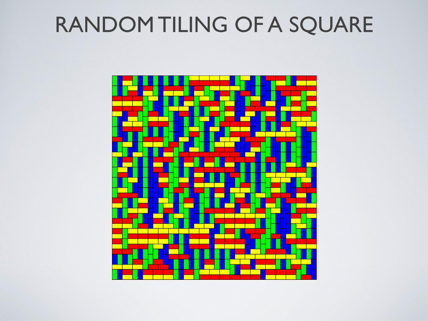
RANDOM TILING OF A SQUAREUniform domino tilings The two-periodic model A few words about the proof

The model: uniform tiling of a planar region by dominos

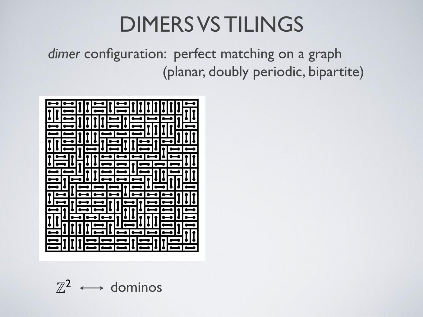
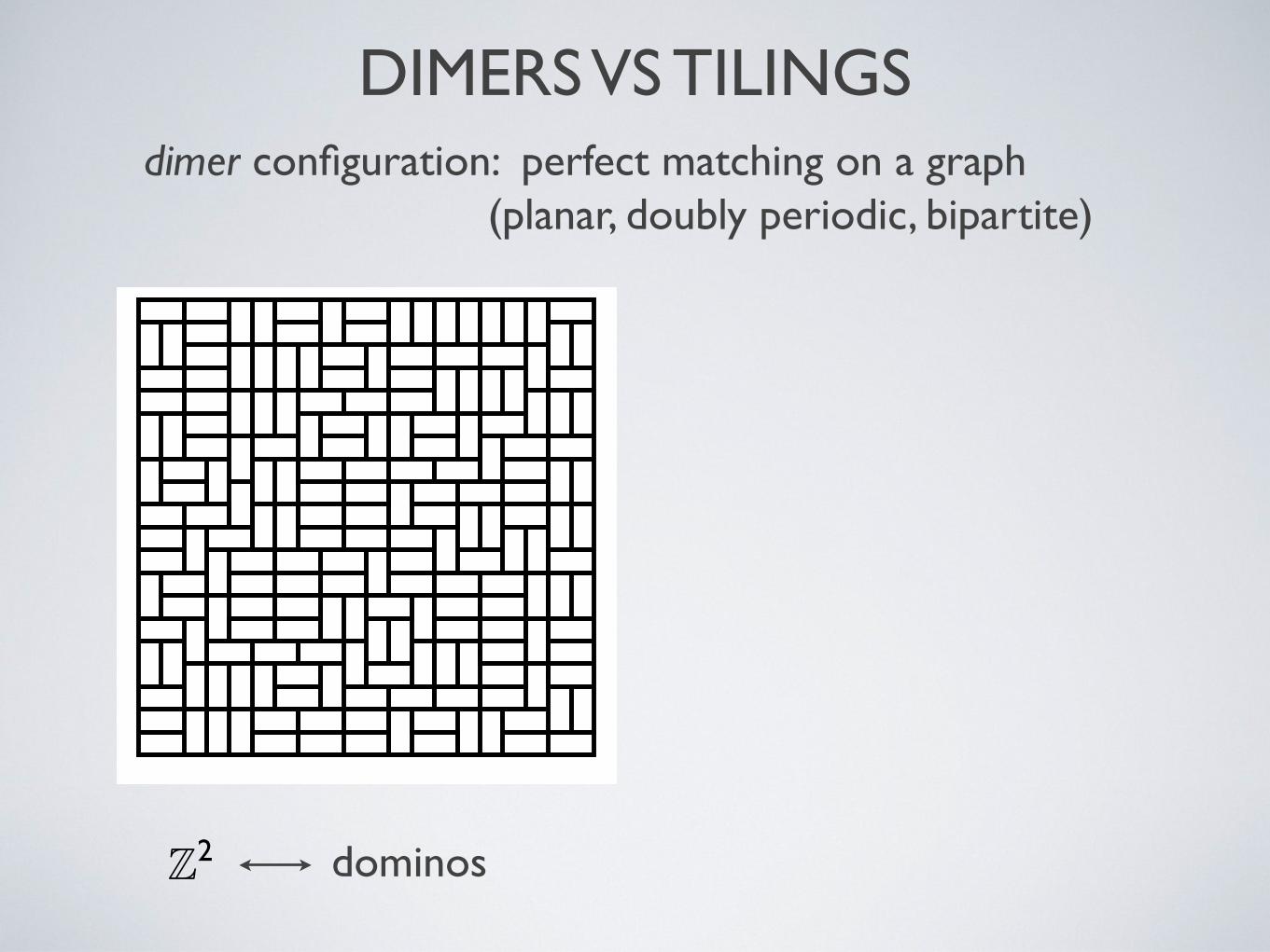
DIMERS VS TILINGS

Dimer model on Z2

P (z, w) = 1 + z + w ! zw

Similar results hold for other (bipartite periodic planar) graphs

dimer configuration: perfect matching on a graph

Z dominos

(planar, doubly periodic, bipartite)

DIMERS VS TILINGS

Dimer model on Z2

P (z, w) = 1 + z + w ! zw


Dimer model on Z2


Z dominos


DIMERS VS TILINGS

Dimer model on Z2

P (z, w) = 1 + z + w ! zw


Dimer model on Z2

Domino tiling model

Dimer model on Z2

Number of tilings = exp(! Area)

! =1

(2"i)2

! !log(1 + z + w ! zw)

dz

z

dw

w.

where

|z| = |w| = 1


Z dominos


DIMERS VS TILINGS

Dimer model on Z2

P (z, w) = 1 + z + w ! zw


Dimer model on Z2

Domino tiling model

Dimer model on Z2

Number of tilings = exp(! Area)

! =1

(2"i)2

! !log(1 + z + w ! zw)

dz

z

dw

w.

where

|z| = |w| = 1


Z dominos

“Lozenge” tilings

dimer model on honeycomb graphhoneycomb lattice rhombus

tilings


THE ARCTIC CIRCLE AGAINCohn-Larsen-Propp

4

HENRYCOHN, MIC

HAELLARSE

N, ANDJA

MESPROPP

Figure

2.A

random

lozeng

e tiling

ofa 32,

32,32

hexago

n.

oneobs

erves

is that the

centra

l zone is rou

ghly cir

cular,

andtha

t thetile

densiti

es

vary con

tinuou

slyexc

eptnea

r themidp

oints

ofthe

sides

ofthe

origin

alhex

agon.

Onecan

inthe

oryuse

ourres

ults to

obtain

anexp

licit for

mulafor

thetyp

ical

shape of

theboun

ding sur

face,

inwhic

h onespeci

fiesthe

distan

cefro

ma poin

t P

onthe

surfac

e toits

image

P! un

derpro

jectio

n onto the

x + y + z =0 pla

ne,as

a

functi

onof

P! ; how

ever, the

integr

altha

t turns

upis qu

itemess

y (albeit

evalua

ble

inclo

sedfor

m), withthe

result

that the

explici

t formula

is extrem

elylen

gthy and

unenl

ighten

ing. Neve

rthele

ss,we can

anddo

give a fai

rlysim

plefor

mulafor

the

tiltof

thetan

gent pla

neat

Pas

a functi

onof

thepro

jectio

n P! , whic

h would

allow one

torec

onstru

ctthe

surfac

e itself.

Invie

wof

thecor

respond

ence betw

een

plane

partiti

onsand

tilings

, specifyi

ngthe

tiltof

thetan

gent pla

neis

equiva

lent

tospeci

fying

theloc

alden

sities

ofthe

three

di!ere

ntori

entati

onsof

lozeng

esfor

random

tilings

ofan

a, b, c

hexago

n.

Ourres

ulton

local

densiti

eshas

asa par

ticula

r corolla

rythe

assert

iontha

t, in

anasy

mptotic

sense,

thezon

e ofmixe

d orient

ation

(defin

edas

thereg

ionin

which

allthr

eeori

entati

onsof

lozeng

e occur

withposi

tive den

sity) is pre

cisely

theint

erior

ofthe

ellipse

inscri

bedin

thehex

agon.

Thisbeha

vior is

analog

ousto

whathas

beenpro

vedcon

cernin

g domino

tilings

ofreg

ions cal

ledAzte

c diamond

s (see [JP

S]

and[CEP]);

these

arerou

ghly squ

arereg

ions, and

if onetile

s them

random

lywith

domino

s (1! 2 rec

tangle

s),the

n thezon

e ofmixe

d orient

ation

tends

inthe

limit

tothe

inscri

beddis

k.How

ever, the

know

n result

s forAzte

c diamond

s arestr

onger

than the

corres

ponding

bestkn

own res

ults for

hexago

ns(se

e Conject

ure6.2

in

Sectio

n 6).

THE ARCTIC CIRCLE AGAINCohn-Larsen-Propp

4

HENRYCOHN, MIC

HAELLARSE

N, ANDJA

MESPROPP

Figure

2.A

random

lozeng

e tiling

ofa 32,

32,32

hexago

n.

oneobs

erves

is that the

centra

l zone is rou

ghly cir

cular,

andtha

t thetile

densiti

es

vary con

tinuou

slyexc

eptnea

r themidp

oints

ofthe

sides

ofthe

origin

alhex

agon.

Onecan

inthe

oryuse

ourres

ults to

obtain

anexp

licit for

mulafor

thetyp

ical

shape of

theboun

ding sur

face,

inwhic

h onespeci

fiesthe

distan

cefro

ma poin

t P

onthe

surfac

e toits

image

P! un

derpro

jectio

n onto the

x + y + z =0 pla

ne,as

a

functi

onof

P! ; how

ever, the

integr

altha

t turns

upis qu

itemess

y (albeit

evalua

ble

inclo

sedfor

m), withthe

result

that the

explici

t formula

is extrem

elylen

gthy and

unenl

ighten

ing. Neve

rthele

ss,we can

anddo

give a fai

rlysim

plefor

mulafor

the

tiltof

thetan

gent pla

neat

Pas

a functi

onof

thepro

jectio

n P! , whic

h would

allow one

torec

onstru

ctthe

surfac

e itself.

Invie

wof

thecor

respond

ence betw

een

plane

partiti

onsand

tilings

, specifyi

ngthe

tiltof

thetan

gent pla

neis

equiva

lent

tospeci

fying

theloc

alden

sities

ofthe

three

di!ere

ntori

entati

onsof

lozeng

esfor

random

tilings

ofan

a, b, c

hexago

n.

Ourres

ulton

local

densiti

eshas

asa par

ticula

r corolla

rythe

assert

iontha

t, in

anasy

mptotic

sense,

thezon

e ofmixe

d orient

ation

(defin

edas

thereg

ionin

which

allthr

eeori

entati

onsof

lozeng

e occur

withposi

tive den

sity) is pre

cisely

theint

erior

ofthe

ellipse

inscri

bedin

thehex

agon.

Thisbeha

vior is

analog

ousto

whathas

beenpro

vedcon

cernin

g domino

tilings

ofreg

ions cal

ledAzte

c diamond

s (see [JP

S]

and[CEP]);

these

arerou

ghly squ

arereg

ions, and

if onetile

s them

random

lywith

domino

s (1! 2 rec

tangle

s),the

n thezon

e ofmixe

d orient

ation

tends

inthe

limit

tothe

inscri

beddis

k.How

ever, the

know

n result

s forAzte

c diamond

s arestr

onger

than the

corres

ponding

bestkn

own res

ults for

hexago

ns(se

e Conject

ure6.2

in

Sectio

n 6).

frozen

liquid

LOZENGE TILINGS

xy

x

y

stepped surfacesviewed from (1,1,1)

direction

“vertical height” parametrized by (1,1,1) plane in Cartesian coordinates

height function

∇ ∈ vertices of a triangle N(0,0)

(0,1)

(1,0)

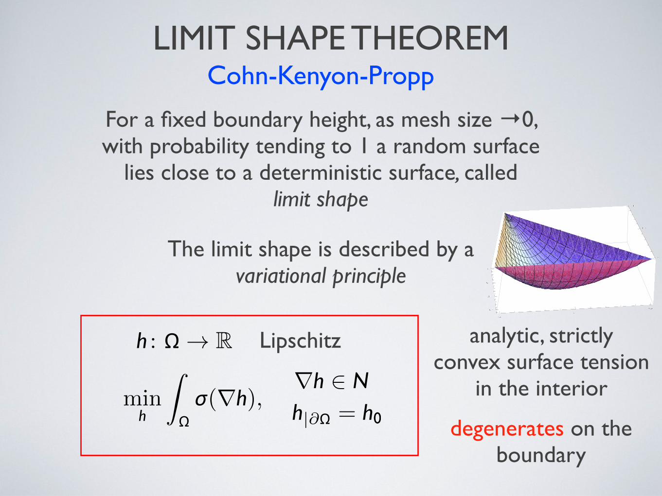
LIMIT SHAPE THEOREMCohn-Kenyon-Propp

min

ˆ(∇ ),

: → R

For a fixed boundary height, as mesh size →0, with probability tending to 1 a random surface

lies close to a deterministic surface, called limit shape

Lipschitz

∇ ∈|∂ =

The limit shape is described by avariational principle

analytic, strictlyconvex surface tension

in the interior

degenerates on the boundary

-2

-1

0

1

2

-2

-1

0

1

2

0

0.5

1

1.5

2

-2

-1

0

1

2

-2 -1.5 -1 -0.5 0.5 1 1.5 2

-2

-1.5

-1

-0.5

0.5

1

1.5

2

Newton polygon = allowed slopes

0.0

0.5

1.0

0.0

0.5

1.0

!0.3

!0.2

!0.1

0.0

surface tension Ronkin functionLegendre duality

Amoeba of P (z, w) = 1 + z + w

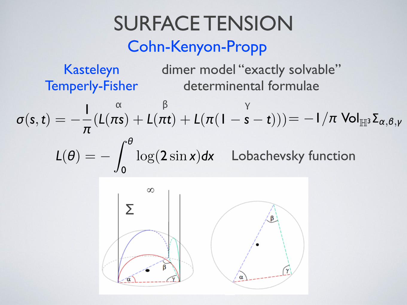
SURFACE TENSION

( , ) = − ( ( ) + ( ) + ( ( − − )))

( ) = −ˆ

log( sin )

= − /H , ,

Lobachevsky function

α β γ

Σ

Cohn-Kenyon-ProppKasteleyn

Temperly-Fisherdimer model “exactly solvable”

determinental formulae

Acta Math., 199 (2007), 263–302

DOI: 10.1007/s11511-007-0021-0

c 2007 by Institut Mittag-Leffler. All rights reserved

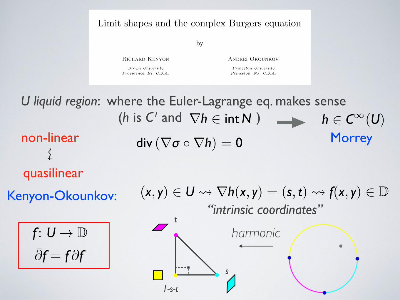
Limit shapes and the complex Burgers equation

by

Richard Kenyon

Brown UniversityProvidence, RI, U.S.A.

Andrei Okounkov

Princeton UniversityPrinceton, NJ, U.S.A.

Contents

1. Introduction . . . . . . . . . . . . . . . . . . . . . . . . . . . . . . . . . . 264

1.1. Overview . . . . . . . . . . . . . . . . . . . . . . . . . . . . . . . . 264

1.2. Random surface models . . . . . . . . . . . . . . . . . . . . . . . 264

1.3. Variational principle . . . . . . . . . . . . . . . . . . . . . . . . . 266

1.4. General planar graphs . . . . . . . . . . . . . . . . . . . . . . . . 266

1.5. Complex Burgers equation . . . . . . . . . . . . . . . . . . . . . 267

1.6. Frozen boundary . . . . . . . . . . . . . . . . . . . . . . . . . . . 269

1.7. Algebraic solutions . . . . . . . . . . . . . . . . . . . . . . . . . . 270

1.8. Reconstruction of limit shape from the Burgers equation . . 271

1.9. Burgers equation in random matrix theory . . . . . . . . . . . 272

1.10. Acknowledgments . . . . . . . . . . . . . . . . . . . . . . . . . . . 272

2. Complex Burgers equation . . . . . . . . . . . . . . . . . . . . . . . . . 273

2.1. Proof of Theorem 1 . . . . . . . . . . . . . . . . . . . . . . . . . 273

2.2. Proof of Corollary 1 . . . . . . . . . . . . . . . . . . . . . . . . . 274

2.3. Complex structure on the liquid region . . . . . . . . . . . . . 274

2.4. Genus of Q . . . . . . . . . . . . . . . . . . . . . . . . . . . . . . . 276

2.5. Islands and bubbles . . . . . . . . . . . . . . . . . . . . . . . . . 276

3. Proof of Theorem 2 . . . . . . . . . . . . . . . . . . . . . . . . . . . . . 280

3.1. Winding curves and cloud curves . . . . . . . . . . . . . . . . . 280

3.2. Inscribing cloud curves in polygons . . . . . . . . . . . . . . . . 283

3.3. Proof of Theorem 3 . . . . . . . . . . . . . . . . . . . . . . . . . 285

4. Global minimality . . . . . . . . . . . . . . . . . . . . . . . . . . . . . . 294

5. Explicit examples . . . . . . . . . . . . . . . . . . . . . . . . . . . . . . . 296

5.1. Disconnected boundary example . . . . . . . . . . . . . . . . . . 296

5.2. Example with a bubble . . . . . . . . . . . . . . . . . . . . . . . 297

5.3. Crystal corner boundary conditions . . . . . . . . . . . . . . . . 298

References . . . . . . . . . . . . . . . . . . . . . . . . . . . . . . . . . . . . . 301

(∇ ∇ ) =

U liquid region: where the Euler-Lagrange eq. makes sense (h is C¹ and )∇ ∈ ∈ ∞( )

non-linear Morrey

Acta Math., 199 (2007), 263–302

DOI: 10.1007/s11511-007-0021-0



by

Richard Kenyon


Andrei Okounkov


Contents

1. Introduction . . . . . . . . . . . . . . . . . . . . . . . . . . . . . . . . . . 264

1.1. Overview . . . . . . . . . . . . . . . . . . . . . . . . . . . . . . . . 264





1.6. Frozen boundary . . . . . . . . . . . . . . . . . . . . . . . . . . . 269






2.1. Proof of Theorem 1 . . . . . . . . . . . . . . . . . . . . . . . . . 273



2.4. Genus of Q . . . . . . . . . . . . . . . . . . . . . . . . . . . . . . . 276


3. Proof of Theorem 2 . . . . . . . . . . . . . . . . . . . . . . . . . . . . . 280



3.3. Proof of Theorem 3 . . . . . . . . . . . . . . . . . . . . . . . . . 285






References . . . . . . . . . . . . . . . . . . . . . . . . . . . . . . . . . . . . . 301

(∇ ∇ ) =


non-linear Morrey

(∇ ∇ ) =

conformal invariance of

(Kenyon-Okounkov)

think

height fluctuations !

Acta Math., 199 (2007), 263–302

DOI: 10.1007/s11511-007-0021-0



by

Richard Kenyon


Andrei Okounkov


Contents

1. Introduction . . . . . . . . . . . . . . . . . . . . . . . . . . . . . . . . . . 264

1.1. Overview . . . . . . . . . . . . . . . . . . . . . . . . . . . . . . . . 264





1.6. Frozen boundary . . . . . . . . . . . . . . . . . . . . . . . . . . . 269






2.1. Proof of Theorem 1 . . . . . . . . . . . . . . . . . . . . . . . . . 273



2.4. Genus of Q . . . . . . . . . . . . . . . . . . . . . . . . . . . . . . . 276


3. Proof of Theorem 2 . . . . . . . . . . . . . . . . . . . . . . . . . . . . . 280



3.3. Proof of Theorem 3 . . . . . . . . . . . . . . . . . . . . . . . . . 285






References . . . . . . . . . . . . . . . . . . . . . . . . . . . . . . . . . . . . . 301

(∇ ∇ ) =


non-linear Morrey

Kenyon-Okounkov:

quasilinear

: → Dt

s

1-s-t

( , ) ∈ ∇ ( , ) = ( , ) ( , ) ∈ D

harmonic

“intrinsic coordinates”

∂ = ∂

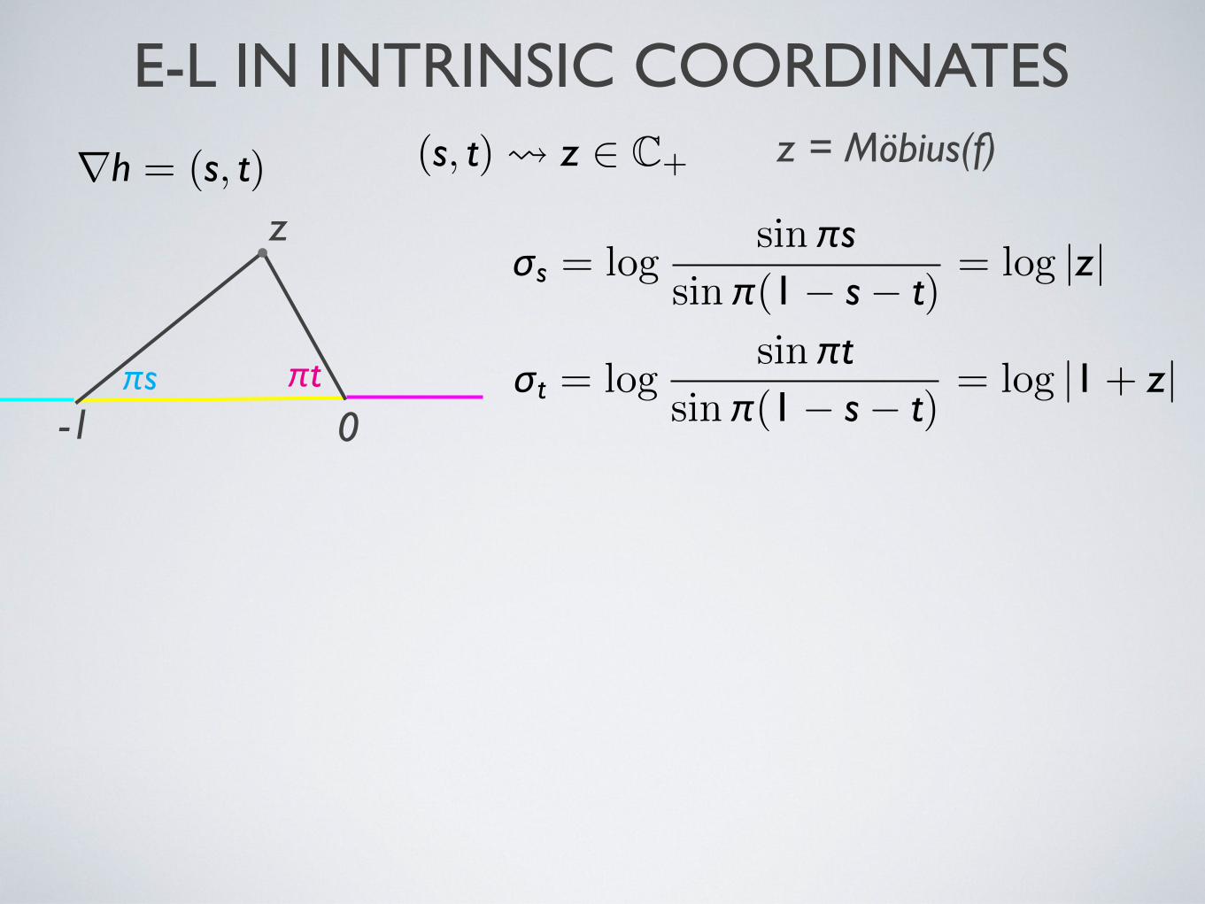
E-L IN INTRINSIC COORDINATES

= logsin

sin ( − − )= log | |

z

-1 0

∇ = ( , ) ( , ) ∈ C+

= logsin

sin ( − − )= log | + |

z = Möbius(f)

E-L IN INTRINSIC COORDINATES

= logsin

sin ( − − )= log | |

z

-1 0

∇ = ( , ) ( , ) ∈ C+

= logsin

sin ( − − )= log | + |

= − arg =

∇ ∇ = (log | |, log | + |)( , ) ∈ → ( , )

++

= (∇ ∇ ) =

+

+

== arg(−( + ))

In terms of f : ∂ = ∂

z = Möbius(f)

ALGEBRAIC CURVES

through volume constraint

cloud curvesinscribed in polygons

deformation argument

limit shapes and the complex burgers equation 293

Figure 15. A cloud curve becomes reducible.

Figure 16. Frozen boundaries (at c<0, c=0 and c>0) for the polygonal region in Figure 6.

The other possibility is when Q degenerates to a union of a winding curve Q1 and

a line Q2. The line Q2 corresponds to a point p2 of the dual plane and the collapsing

ellipse follows the tangent from p2 to Q∨1 ; this is illustrated on the right in Figure 15.

This degeneration can only happen if an edge of Ω has length tending to zero.

Note that in codimension 2 one can have a degeneration in which two cusps of the

frozen boundary come together and merge in a tacnode, reminiscent of Henry Moore’s

Oval with Points. This corresponds in Figure 15, left part, to the thin ellipse having zero

size.

Finally, there is practical side to the above deformation argument. Namely, it allows

us to find the inscribed curve by numeric homotopy, that is, by solving the equations

using Newton’s algorithm with the solution of the nearby problem as the starting point.

An example of a practical implementation of this can be see in Figure 16.

3.3.6. Uniqueness

It remains to prove that the inscribed curve is unique and that the polygon is feasible if

the inscribed curve exists. Given the inscribed curve R, let hdenote the height function

obtained from it by the procedure of §1.8. This is a well-defined function with gradient

in the triangle (1). Therefore Ω is feasible. The inscribed curve is unique because by the

results of §3.3.5 it has a unique deformation to the unique tropical inscribed curve.

Kenyon-Okounkov

polygonal boundarycontour in coordinate

directions

(a solution to Euler-Lagrange exists)

algebraic frozen boundary+ frozen facets

“It would be interesting to prove...”

frozen boundary = free boundary

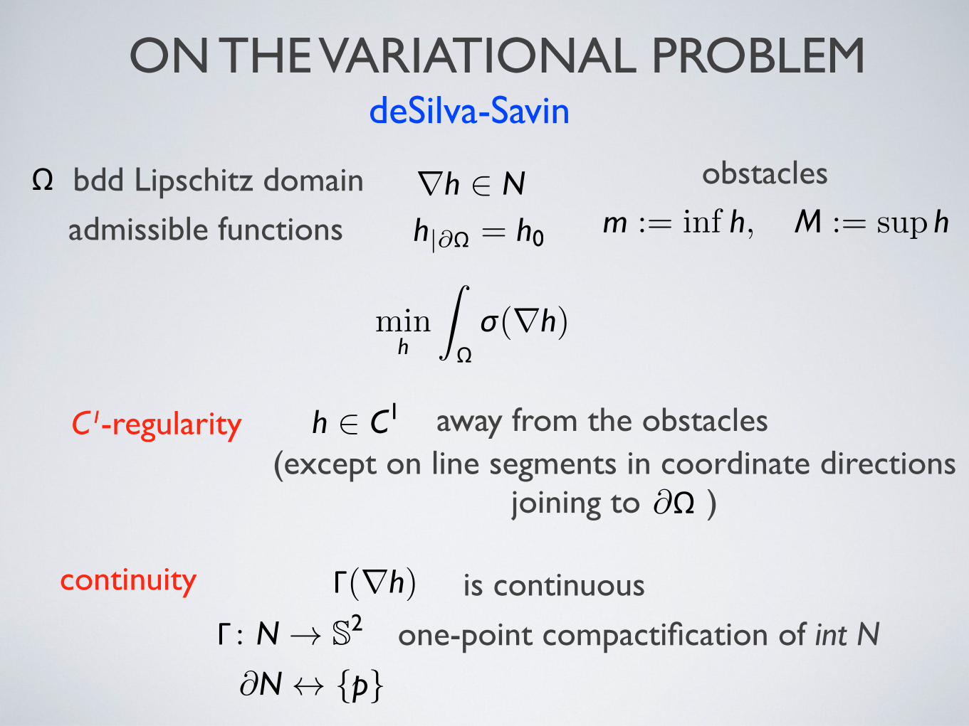
ON THE VARIATIONAL PROBLEMdeSilva-Savin

obstacles∇ ∈|∂ =admissible functions := inf , := sup

C¹-regularity ∈ away from the obstacles(except on line segments in coordinate directions

joining to )∂

bdd Lipschitz domain

continuity is continuous(∇ )

: → S one-point compactification of int N

min

ˆ(∇ )

∂ ↔

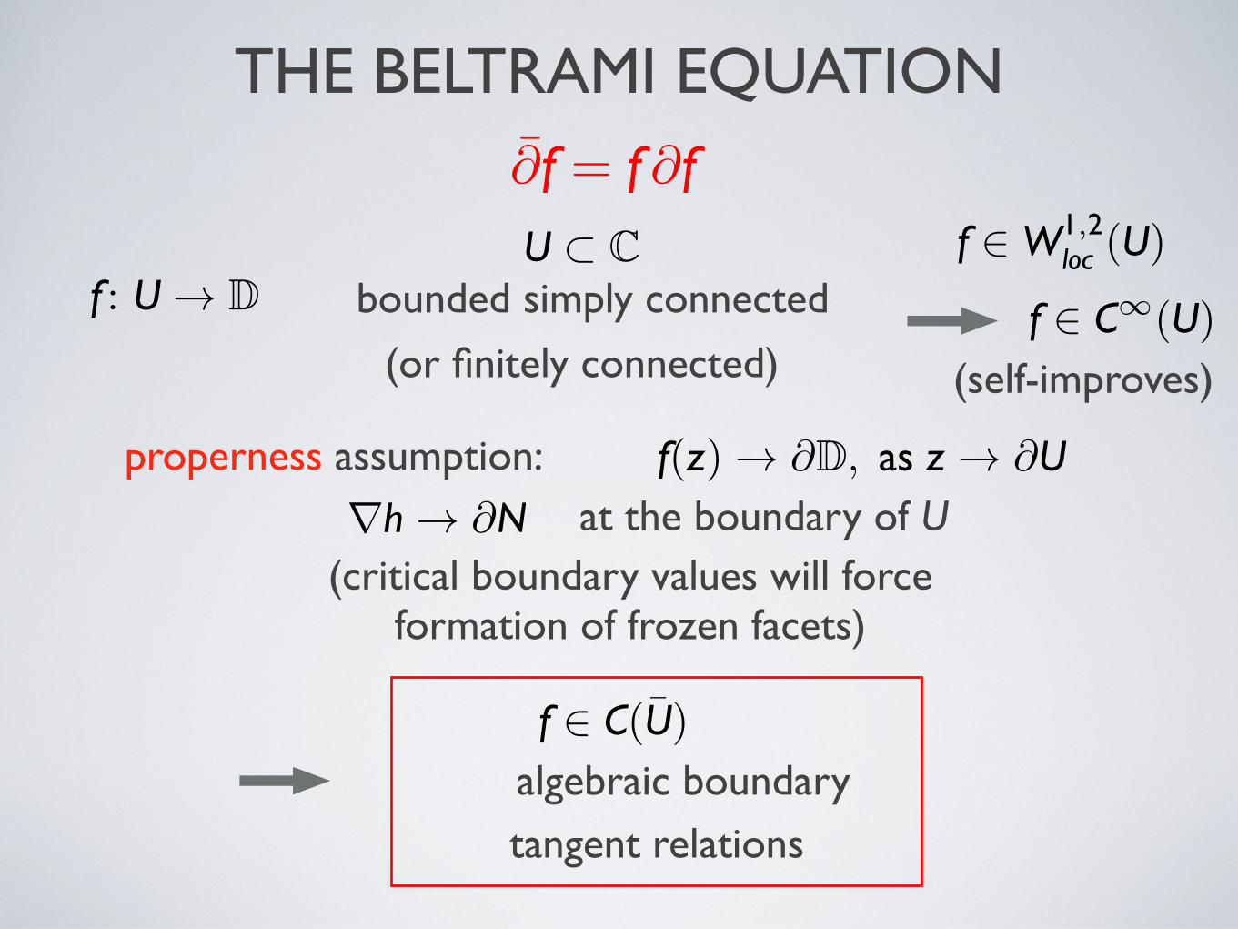
THE BELTRAMI EQUATION∂ = ∂

: → D ∈ ∞( )

∈ , ( )

properness assumption:

⊂ Cbounded simply connected

(or finitely connected)

( ) → ∂D, → ∂

∈ (¯)

(self-improves)

∇ → ∂

algebraic boundarytangent relations

at the boundary of U(critical boundary values will force

formation of frozen facets)

INVERSE MAP= −

: D → homeomorphism ∂ = − ( )∂

: D → D analytic + proper finite Blaschke product

= + ¯ is holomorphic in D

( − | | ) = − ¯

( )− ( ) ( ) → , → ∈ ∂D( ) = ( ) ( ) =

( )

( )

extend by reflection ( ) = ( ) ( /¯)

h is a rational map of C

( )− ( /¯) → , | | → weakly across

( ) = ( /¯)

∂D∂ =

UNIVALENT POLYNOMIALS( ) = ,

h is a polynomial of degree d-1

( ) = ( /¯), ( ) =

self-reflective

( ) =( )− ( )

− | | ( ) = ( ), ∈ ∂D( ) = ( )− ( )

extends continously to the boundary

( ) = + . . .+ ¯ −

( ) = ( − ) + . . .+ ( − )¯ −

(∂D) non self-crossing curvep is univalent in D

all d-2 critical points are on ∂D − ( /¯) = ( )

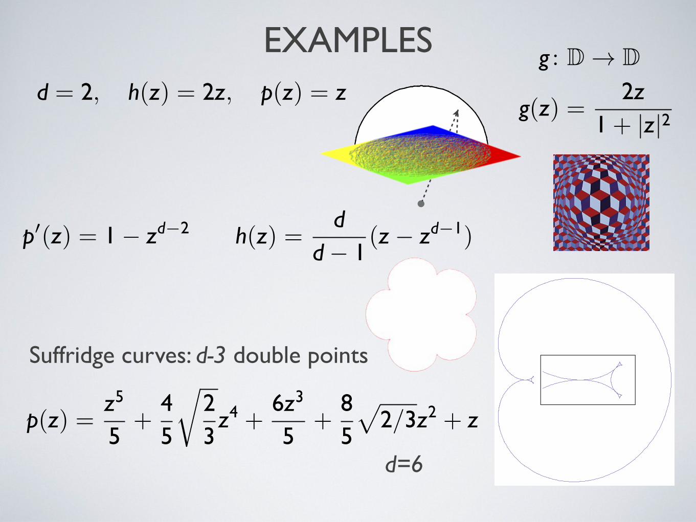
EXAMPLES

Suffridge curves: d-3 double points

d=6

= , ( ) = , ( ) =

( ) = − ( − − )( ) = − −

( ) = +

+ +

/ +

Definition. f ∈ (Sd) is a Suffridge polynomial if the quadrature domain f(D) is extreme, i.e. it has themaximal number of singularities: d − 1 cusps and d − 2 double points. The curve f(T) is a Suffridgecurve.

Examples of Suffridge curves (see Figure 2 and 3):

(a) d = 2: The only (up to rotation) Suffridge polynomial in (S2) is

f(z) = z +z2

2.

The corresponding curve is the cardioid.

(b) d = 3 (Kossler ‘51 [14]; Cowling, Royster ’67 [6]; Brannan ’67 [4]):

f(z) = z +2√2

3z2 +

z3

3.

This polynomial simultaneously maximizes |a2| and |a3| in (S3).

(c) d = 4 (C. Michel ’70 [1])

f(z) = z +3

2A eitz2 +A e−itz3 +

z4

4,

where A = 12

3√

15− 3and t = 1

3 cos−1

316

9 + 5

√15.

(d) d = 5: This polynomial corresponds to the third picture in Figure 2.

f(z) =z5

5+

4

5

2

3z4 +

6z3

5+

8

5

2

3z2 + z.

(e) d = 6 and d = 7: The curves in Figure 3 were obtained numerically.

Figure 2: Suffridge curves for d = 3, d = 4, d = 5 and d = 5 (from left to right). The boxed insets arezoomed images of the singularities.

Let us define(S∗

d) = f ∈ (Sd) | ad = 1/d

7

( ) =+ | |

: D → D

On the ceiling of the burial chamber visitors can marvel at one outstandingexample of 4th Century Early Christian wall painting. The painting symbolizingparadise has a rich plant (grapes) and animal (peacock) ornament and the picturesof four young people - whose characters are unknown - cased in medallions. Hereyou can find 6 pictures with biblical theme.

The Korsós ’Pitcher’ burial chamber was also discovered during the estab-lishment of the extensive Pécs cellar system in the 18th century. The chamber gotits name from the pitcher and glass symbols that are found in the box in its northernwall. Plant and geometric decorations can be seen on the walls and the rail motifprobably refers to the garden of paradise.

VASARELY MUSEUM

Address: 3 Káptalan Street. Opening hours: Tuesday-Sunday 10 a.m - 18 p.m.Mondays closed. This is a recommended program for the afternoon of 30th.

The Vasarely Museum is one of Pécs’ most popular collections.


Vasarely was born in Pécs underthe name Vásárhelyi Győző, grew up inPöstyén (now in Slovakia) and Budapestand settled in Paris in 1930. He died age90 in Paris in 1997. Vasarely producedart and sculpture using optical illusion.This Hungarian–French artist is widelyaccepted as a "grandfather" and leaderof the op art movement. His work enti-tled Zebra, created in the 1930s, is con-sidered by some to be one of the earliestexamples of op art. (You can find this

piece of art in the museum.) He developed his style of geometric abstract art, work-ing in various materials but using a minimal number of forms and colors. Vasarelyexperimented with textural effects, perspective, shadow and light. Beginning from1947 he started to develop geometric abstract art (optical art) and finally, Vasarelyfound his own style. He worked on the problem of empty and filled spaces on a flatsurface as well as the stereoscopic view.

(Op art, short for optical art, is a style of visual art that uses optical illusions.Op art works are abstract, with many better known pieces created in black andwhite. Typically, they give the viewer the impression of movement, hidden images,flashing and vibrating patterns, or of swelling or warping.)


Kinetic images, black-white pho-tographies: He then created kinetic im-ages in black-white which create dy-namic, moving impressions dependingon the viewpoint. In the black-white pe-riod he combined the frames into a sin-gle pane by transposing photographiesin two colors. Building on the researchof constructivist and Bauhaus pioneers,he postulated that visual kinetics (plas-tique cinétique) relied on the perceptionof the viewer who is considered the solecreator, playing with optical illusions.

55

RATIONAL PARAMETRIZATION

( ) =( )− ( ) ( )

− | ( )| =

( )( ) − ( )

( ) − ( )=

( )( ) −

( /¯)( /¯)

( ) − ( /¯)

→ ( ), → ∈ ∂D =( / )

( / )( /¯) =

( ) self-reflective with respect to B(z)

( ) ( /¯) = ( )

boundary is algebraic & locally convex except at d-2 cusps

= − continuous up to the boundary

tangent vector ( ) = ( )

( )

d/2 − 1/2 # cusps =1 real, sign changes at cusps

3d-3 real parameters

BOUNDARY RECONSTRUCTION

f

limit shapes and the complex burgers equation

293

Figure 15. A cloud curve becomes reducible.

Figure 16. Frozen boundaries (at c<0, c=0 and c>0) for the polygonal region in Figure 6.

Theother possibility

is when Qdegenerates to

aunion

of awinding

curve Q1 and

aline Q

2 .The

line Q2 corresponds to

apoint p2 of the

dual planeand

thecollapsing

ellipsefollows the

tangent from p2 to Q ∨1 ; this is illustrated

onthe

right inFigure

15.

This degenerationcan

onlyhappen

if anedge of Ω

has lengthtending

tozero.

Note that incodim

ension2one can

have adegeneration

inwhich

twocusps of the

frozenboundary

cometogether and

merge

inatacnode, rem

iniscent of HenryMoore’s

Oval with Points. This corresponds inFigure 15, left part, to the thin

ellipse having zero

size.

Finally, there is practical side to the above deformation

argument. Nam

ely, it allows

us tofind

theinscribed

curveby

numerichomotopy, that is, by

solvingthe

equations

usingNewton’s algorithm

withthe solution

of the nearbyproblem

as the startingpoint.

Anexam

ple of apractical im

plementation

of this canbe see in

Figure 16.

3.3.6. Uniqueness

It remains to

prove that the inscribedcurve is unique and

that the polygonis feasible if

the inscribedcurve exists. Given

the inscribedcurve R, let h

denote the height function

obtainedfrom

it bythe procedure of §1.8. This is a

well-definedfunction

withgradient

inthe triangle (1). Therefore Ω

is feasible. The inscribedcurve is unique because by

the

results of §3.3.5it has a

unique deformation

tothe unique tropical inscribed

curve.

MULTIPLY CONNECTED CASE

D D circle domain

B and h continuous up to the boundary as before

: D → D analytic and proper

( ) = ( ) ( ) =( )

( ), ∈ ∂D

( , / ) are meromorphic functions on the Schottky double D( , / )

˜=

,( / )

( / )

j antiholomorphic involution

=˜

= −

meromorphic functions

( ) = ( ), ∈ ∂D( , ) =

algebraic boundary etc

( ( ), ( )) =

J. Phys. A: Math. Theor. 47 (2014) 285204 P Di Francesco and R Soto-Garrido

!1 = 4/9 !1 = 1/5 !1 = 19/10 !1 = 200/201

Figure 13. Arctic curves for the 3-toroidal initial data corresponding to different valuesof !1, where !0 = 1/2, !2 = 1 ! !1 and µ0 = µ1 = µ2 = 1/2.

µ1 = 1/5 µ1 = 2/3 µ1 = 9/10 µ1 = 99/100

Figure 14. Arctic curves for the 3-toroidal initial data corresponding to different valuesof µ1. Where !0 = 1/2, !1 = 1/4, !2 = 1 ! !1 = 3/4, µ0 = 1/2 and µ2 = 1 ! µ1.

(a) (b)

Figure 15. Typical dominant states for the 3-toroidal partition function, in the caseswhere: (a) c0 " 0 while all other face weights remain finite (we have shaded thec0-type faces); and (b) c0 # d1 " 0 while all other face weights remain finite (bothtypes of faces are shaded).

without overall scaling otherwise. We have represented the profiles of the density functionk"(0,0)

i, j,k for size k = 77 in figure 16.

4.3.2. Case m = 4. The structure of phases is similar to the cases m = 2, 3, except that wenow have three inner facet regions along the diagonal of the square domain. As before, we

25

Journal of Physics A: Mathematical and Theoretical

J. Phys. A: Math. Theor. 47 (2014) 285204 (34pp) doi:10.1088/1751-8113/47/28/285204

Arctic curves of the octahedron equation

Philippe Di Francesco1 and Rodrigo Soto-Garrido2

1 Department of Mathematics, University of Illinois at Urbana-Champaign, MC-382,1409 W Green St., Urbana, IL 61801, USA2 Department of Physics, University of Illinois at Urbana-Champaign,1110 W Green St., Urbana, IL 61801, USA

E-mail: [email protected] and [email protected].

Received 18 February 2014, revised 30 May 2014Accepted for publication 4 June 2014Published 30 June 2014

AbstractWe study the octahedron relation (also known as the A! T -system), obeyed inparticular by the partition function for dimer coverings of the Aztec Diamondgraph. For a suitable class of doubly periodic initial conditions, we find exactsolutions with a particularly simple factorized form. For these, we showthat the density function that measures the average dimer occupation of aface of the Aztec graph, obeys a system of linear recursion relations withperiodic coefficients. This allows us to explore the thermodynamic limit of thecorresponding dimer models and to derive exact ‘arctic’ curves separating thevarious phases of the system.

Keywords: arctic curve, dimer, tiling, exact solution, phase transitionPACS numbers: 64.60.De, 64.70.qd, 02.10.Ox

(Some figures may appear in colour only in the online journal)

1. Introduction

The octahedron recurrence is a system of nonlinear equations describing the evolution of aquantity Ti, j,k, i, j, k " Z corresponding to discrete space (i, j) and time k. This equation firstarose in the context of integrable quantum spin chains with a Lie group symmetry [32, 33], andis obeyed by the corresponding quantum transfer matrices. In this language, the octahedronequation corresponds to the so-called T -system (for A!). In this formulation, the indicesi, k, j respectively stand for representation indices, and a discrete spectral parameter. The A-type T -systems have remarkable properties, depending on the choice of boundary conditions,such as discrete integrability [15], and periodicity properties [16, 23] as well as the positiveLaurent property (solutions are Laurent polynomials of the initial data with non-negativeinteger coefficients) in relation to cluster algebras [11].

1751-8113/14/285204+34$33.00 © 2014 IOP Publishing Ltd Printed in the UK 1


!1 = 4/9 !1 = 1/5 !1 = 19/10 !1 = 200/201

Figure 13. Arctic curves for the 3-toroidal initial data corresponding to different valuesof !1, where !0 = 1/2, !2 = 1 ! !1 and µ0 = µ1 = µ2 = 1/2.

µ1 = 1/5 µ1 = 2/3 µ1 = 9/10 µ1 = 99/100

Figure 14. Arctic curves for the 3-toroidal initial data corresponding to different valuesof µ1. Where !0 = 1/2, !1 = 1/4, !2 = 1 ! !1 = 3/4, µ0 = 1/2 and µ2 = 1 ! µ1.

(a) (b)

Figure 15. Typical dominant states for the 3-toroidal partition function, in the caseswhere: (a) c0 " 0 while all other face weights remain finite (we have shaded thec0-type faces); and (b) c0 # d1 " 0 while all other face weights remain finite (bothtypes of faces are shaded).

without overall scaling otherwise. We have represented the profiles of the density functionk"(0,0)

i, j,k for size k = 77 in figure 16.

4.3.2. Case m = 4. The structure of phases is similar to the cases m = 2, 3, except that wenow have three inner facet regions along the diagonal of the square domain. As before, we

25

Journal of Physics A: Mathematical and Theoretical

J. Phys. A: Math. Theor. 47 (2014) 285204 (34pp) doi:10.1088/1751-8113/47/28/285204

Arctic curves of the octahedron equation

Philippe Di Francesco1 and Rodrigo Soto-Garrido2

1 Department of Mathematics, University of Illinois at Urbana-Champaign, MC-382,1409 W Green St., Urbana, IL 61801, USA2 Department of Physics, University of Illinois at Urbana-Champaign,1110 W Green St., Urbana, IL 61801, USA

E-mail: [email protected] and [email protected].

Received 18 February 2014, revised 30 May 2014Accepted for publication 4 June 2014Published 30 June 2014

AbstractWe study the octahedron relation (also known as the A! T -system), obeyed inparticular by the partition function for dimer coverings of the Aztec Diamondgraph. For a suitable class of doubly periodic initial conditions, we find exactsolutions with a particularly simple factorized form. For these, we showthat the density function that measures the average dimer occupation of aface of the Aztec graph, obeys a system of linear recursion relations withperiodic coefficients. This allows us to explore the thermodynamic limit of thecorresponding dimer models and to derive exact ‘arctic’ curves separating thevarious phases of the system.

Keywords: arctic curve, dimer, tiling, exact solution, phase transitionPACS numbers: 64.60.De, 64.70.qd, 02.10.Ox

(Some figures may appear in colour only in the online journal)

1. Introduction

The octahedron recurrence is a system of nonlinear equations describing the evolution of aquantity Ti, j,k, i, j, k " Z corresponding to discrete space (i, j) and time k. This equation firstarose in the context of integrable quantum spin chains with a Lie group symmetry [32, 33], andis obeyed by the corresponding quantum transfer matrices. In this language, the octahedronequation corresponds to the so-called T -system (for A!). In this formulation, the indicesi, k, j respectively stand for representation indices, and a discrete spectral parameter. The A-type T -systems have remarkable properties, depending on the choice of boundary conditions,such as discrete integrability [15], and periodicity properties [16, 23] as well as the positiveLaurent property (solutions are Laurent polynomials of the initial data with non-negativeinteger coefficients) in relation to cluster algebras [11].

1751-8113/14/285204+34$33.00 © 2014 IOP Publishing Ltd Printed in the UK 1


Appendix. m = 3 and m = 4 arctic curves

In this appendix we include explicit expressions for the limit shape curves for the cases m = 3and m = 4. We only give the expression for a specific value of the parameters, since theexpressions are in general very cumbersome.• Arctic curve for m = 3 with !0 = 1/2, !1 = 1/4, !2 = 3/4, µ0 = 1/2, µ1 = 1/5 and

µ2 = 4/5. This corresponds to the left most curve in figure 14.P(u, v) = 603 358 073 569 688 095 393 738 000u14 + 1822 971 422 522 481 873 814 304 800vu13 + 302 414 835 014 281 399 576 977 600u13

+ 7658 013 562 515 635 323 215 886 000v2u12 + 626 386 479 045 976 264 625 165 760vu12 + 65 648 625 922 043 130 480 407 960u12

+ 8502 660 801 885 990 861 442 260 800v3u11 ! 4016 291 377 989 674 598 197 523 840v2u11 ! 8955 889 812 423 159 779 663 425 824vu11

! 648 516 348 371 464 166 524 636 080u11 + 24 870 815 123 962 290 558 144 794 000v4u10 ! 961 218 355 287 663 519 951 292 800v3u10

! 6515 407 606 857 043 381 218 037 200v2u10 ! 172 367 781 226 698 452 854 372 560vu10 + 1099 108 080 544 208 467 044 202 281u10

+ 8664 424 609 796 383 599 417 068 000v5u9 ! 17 028 590 399 764 390 279 389 912 000v4u9 ! 11 010 604 932 056 552 215 403 730 080v3u9

+ 8631 816 024 097 405 173 283 346 160v2u9 + 6130 342 332 781 365 103 023 636 918vu9 + 300 038 159 586 641 951 467 587 240u9

+ 48 101 067 368 389 417 583 947 124 400v6u8 ! 8874 912 221 343 735 420 641 284 800v5u8 ! 30 642 500 612 723 566 034 952 420 120v4u8

+ 4089 814 979 226 593 490 453 920 400v3u8 + 2890 833 100 949 061 663 021 542 421v2u8 ! 1537 862 122 247 709 326 673 670 200vu8

! 1276 791 684 735 224 437 145 235 252u8 + 165 638 160 476 224 209 249 648 000v7u7 ! 15 185 547 478 970 793 846 022 129 920v6u7

+ 10 619 324 480 232 243 252 222 805 440v5u7 + 17 121 927 414 923 400 963 351 428 640v4u7 ! 4642 084 019 946 561 205 079 466 936v3u7

! 4201 308 893 745 605 384 096 673 600v2u7 + 97 128 658 780 698 750 571 038 384vu7 + 16 658 271 644 450 437 458 125 640u7

+ 48 101 067 368 389 417 583 947 124 400v8u6 ! 15 185 547 478 970 793 846 022 129 920v7u6 ! 54 696 534 109 775 129 942 931 200 352v6u6

+ 8498 087 480 515 562 992 290 313 440v5u6 + 20 848 735 934 263 779 279 940 738 242v4u6 ! 2928 090 072 842 649 426 783 830 400v3u6

! 1125 942 030 946 106 640 101 862 864v2u6 + 881 693 827 811 784 667 334 364 120vu6 + 410 818 358 444 129 895 320 450 118u6

+ 8664 424 609 796 383 599 417 068 000v9u5 ! 8874 912 221 343 735 420 641 284 800v8u5 + 10 619 324 480 232 243 252 222 805 440v7u5

+ 8498 087 480 515 562 992 290 313 440v6u5 ! 16 598 910 777 434 586 615 901 305 852v5u5 ! 3118 943 690 894 703 413 913 413 040v4u5

+ 4436 727 620 735 139 576 883 870 032v3u5 + 378 779 090 210 933 672 213 353 800v2u5 ! 894 275 420 028 329 313 474 734 772vu5

! 28 143 830 188 642 461 399 955 080u5 + 24 870 815 123 962 290 558 144 794 000v10u4 ! 17 028 590 764 390 279 389 912 000v9u4

! 30 642 500 723 566 034 952 420 120v8u4 + 17 121 927 923 400 963 351 428 640v7u4 + 20 848 735 263 779 279 940 738 242v6u4

! 3118 943 690 894 703 413 913 413 040v5u4 ! 6585 025 120 215 513 060 415 620 600v4u4 + 224 576 822 600 011 254 994 156 440v3u4

+ 730 062 356 407 169 871 489 508 026v2u4 ! 87 999 348 446 432 687 845 418 760vu4 ! 39 991 576 579 826 072 416 315 884u4

+ 8502 660 801 885 990 861 442 260 800v11u3 ! 961 218 355 287 663 519 951 292 800v10u3 ! 11 010 604 932 056 552 215 403 730 080v9u3

+ 4089 814 979 226 593 490 453 920 400v8u3 ! 4642 084 019 946 561 205 079 466 936v7u3 ! 2928 090 072 842 649 426 783 830 400v6u3

+ 4436 727 620 735 139 576 883 870 032v5u3 + 224 576 822 600 011 254 994 156 440v4u3 ! 771 752 886 154 129 578 670 446 744v3u3

+ 54 105 975 565 681 638 845 373 840v2u3 + 158 742 939 499 283 087 522 192 736vu3 + 3181 828 983 737 934 822 021 000u3

+ 7658 013 562 515 635 323 215 886 000v12u2 ! 4016 291 377 989 674 598 197 523 840v11u2 ! 6515 407 606 857 043 381 218 037 200v10u2

+ 8631 816 024 097 405 173 283 346 160v9u2 + 2890 833 100 949 061 663 021 542 421v8u2 ! 4201 308 893 745 605 384 096 673 600v7u2

! 1125 942 030 946 106 640 101 862 864v6u2 + 378 779 090 210 933 672 213 353 800v5u2 + 730 062 356 407 169 871 489 508 026v4u2

+ 54 105 975 565 681 638 845 373 840v3u2 ! 205 856 416 682 486 477 443 753 704v2u2 ! 4541 013 871 098 771 634 821 000vu2

! 417 838 190 775 940 873 949 175u2 + 1822 971 422 522 481 873 814 304 800v13u + 626 386 479 045 976 264 625 165 760v12u

! 8955 889 812 423 159 779 663 425 824v11u ! 172 367 781 226 698 452 854 372 560v10u + 6130 342 332 781 365 103 023 636 918v9u

! 1537 862 122 247 709 326 673 670 200v8u + 97 128 658 780 698 750 571 038 384v7u + 881 693 827 811 784 667 334 364 120v6u

! 894 275 420 028 329 313 474 734 772v5u ! 87 999 348 446 432 687 845 418 760v4u + 158 742 939 499 283 087 522 192 736v3u

! 4541 013 871 098 771 634 821 000v2u + 925 709 140 319 743 466 938 350vu ! 636 257 259 784 396 800 000u

+ 603 358 073 569 688 095 393 738 000v14 + 302 414 835 014 281 399 576 977 600v13 + 65 648 625 922 043 130 480 407 960v12

! 648 516 348 371 464 166 524 636 080v11 + 1099 108 080 544 208 467 044 202 281v10 + 300 038 159 586 641 951 467 587 240v9

! 1276 791 684 735 224 437 145 235 252v8 + 16 658 271 644 450 437 458 125 640v7 + 410 818 358 444 129 895 320 450 118v6

! 28 143 830 188 642 461 399 955 080v5 ! 39 991 576 579 826 072 416 315 884v4 + 3181 828 983 737 934 822 021 000v3

! 417 838 190 775 940 873 949 175v2 ! 636 257 259 784 396 800 000v + 6507 176 520 522 240 000.

31

LIFE BEYOND THE ARCTIC CIRCLE

arctic curves beyond the arctic circlefourier2017.ttk.pte.hu/files/slides/prause.pdf · of...

Documents