archives - pdfs.semanticscholar.org · three essays in law and economics by joshua b. fischman...
TRANSCRIPT

Three Essays in Law and Economics
by
Joshua B. Fischman
A.B., Princeton University (1994)J.D., Yale University (1999)
Submitted to the Department of Economicsin partial fulfillment of the requirements for the degree of
Doctor of Philosophy
at the
MASSACHUSETTS INSTI
Y
MASAHUETSINS1TTEMASSACHUSETTS INSTMITE
OF TECHNOLOGY
SEP 2 5 2006
LIBRARIES
September 2006
ARCHIVES@ Joshua B. Fischman 2006
The author hereby grants to Massachusetts Institute of Technology permission toreproduce and
to distribute copies of this thesis document in whole or in part.
Signature of Author..
Certified by .................................---.
Deartment of Economics20 September 2006
Glenn EllisonProfessor of Economics
Thesis Supervisor
Accepted by ....................................................Peter Temin
Elisha Gray II Professor of Economics
=IP

Three Essays in Law and Economics
byJoshua B. Fischman
Submitted to the Department of Economicson 20 September 2006, in partial fulfillment of the
requirements for the degree ofDoctor of Philosophy
Abstract
The first chapter presents a model of legal interpretation in a hierarchical court. Using atwo-level court in which judges have spatial preferences over doctrine, the model examines howappeals, panels, and other structural features of the court affect the incentives of judges andpromote uniform interpretation of the laws. The threat of appeal has a moderating influence onjudges in the lower court. When the cost of appeal is low, this effect will be stronger, but thelower court will also have less influence on the final decision. Hence, under many conditions,overall uniformity will be maximized at an intermediate cost of review. Factors that mayincrease the predictability of rulings on the higher court, such as panel size, may weaken theincentives toward moderation on the lower court.
The second chapter analyzes judicial decision making in three-judge appellate panels. Whenjudges are ideological but have a preference for consensus, there will be negotiation among thethree judges in an effort to reach agreement. This paper constructs a model of judicial negotia-tion, where judges have preferences on an ideological spectrum and disutility from disagreement.The parameters of the negotiation model and the judges' ideological inclinations are then es-timated on a data set of sex discrimination cases using maximum likelihood estimation. Theresults find strong evidence that judges' votes are influenced by their panel colleagues, but thatthis influence mostly takes the form of outvoted judges joining the majority. However, judgesin the minority appear to have a small but significant effect on case outcomes.
The third chapter examines the impact of liability law on firms' investments in productsafety when such investments take the form of fixed costs and liability does not apply equallyto competing products. Using a model with one innovative good and one competitively suppliedgood, the paper finds that asymmetric liability deters safety innovation when the adminstrationof the tort system is inefficient. When inefficiencies in the tort system are small, however,incentives to develop safer products may be stronger under asymmetric liability.
Thesis Supervisor: Glenn EllisonTitle: Professor of Economics

Acknowledgments
I began graduate school five years ago with very little knowledge of economics. I owe a huge
debt to so many people who have helped me get where I am today.
I am especially grateful to Glenn Ellison, who has been an insightful, patient, and dedicated
thesis advisor. Much of what I know about economics I learned from him. I thank him for
his constant support and encouragement during my time at MIT.
Stephen Ryan provided much guidance for the second chapter of this thesis. I thank him
for his insights, his enthusiasm, and for always being patient when I had another question. I
thank Jim Snyder for offering a useful perspective and for so many helpful conversations and
suggestions.
I thank the Department of Economics at MIT for giving me a chance when I barely knew
anything about economics and for its generous support during the first two years of graduate
school.
I have been fortunate to have been part of an extraordinary intellectual environment at
MIT and to have had so many wonderful classmates. I have learned so much from all them. I
am grateful to Jackie Chou, Liz Ananat, and Sarah Siegel, who helped me get through my first
two years of classes. David Matsa has been a wonderful roommate, office-mate, study partner
and friend. I would also like to thank David Abrams, Marek Pycia, J.J. Prescott, Dominique
Lauga, and Alan Grant for numerous helpful discussions.
I am deeply grateful to my wife, Polly, who gave me so much love and support during these
last five years. She encouraged me to attend graduate school when it still seemed like a crazy
idea, and made many sacrifices so that I could do it. She has endured all of the ups and downs
of graduate life with me, and has been a constant source of strength.
I thank my daughters, Maisie and Josie, for bringing so much joy into my life and for
understanding when I had to spend a lot of time at "Daddy's office." Finally, I wish to thank
my parents, my brother, my sister, and my in-laws for their love, support, and encouragement.
I could not have done this without all of you.

Contents
1 Uniformity of Interpretation in a Hierarchical Court
1.1 Description of the Model ......................
1.2 General Results ......................
1.3 Implications of the Model . ................
1.3.1 Cost of Review ..................
1.3.2 Uncertainty ....................
1.3.3 Aversion to Reversal ...............
1.4 Effects of Court Structure on Interpretation ......
1.5 Conclusion ........................
1.6 Appendix .........................
2 Collegial Decision Making in the Courts of Appeals:
2.1 M odel . . . . . . . . . . . . . . . . . . . . . . . . . . .
2.2 Estim ation ........................
2.3 D ata . . . . . . . . . . . . . . . . . . . . . . . . . . . .
2.4 Results ............ ...........
2.4.1 Judge Preferences ................
2.4.2 Costs of Disagreement ..............
2.5 Sim ulations ........................
2.5.1 Frequency of Compromise ............
2.5.2 Individual Judge vs. Three-Judge Panels . . .
2.6 Conclusion ........................
An
..
..
..
..
..
..
..
..
. .
Empirical
.oo.o.o
.......
.......
.......
.......
.......
o..o..o
...... o
Analysis
......
.. o...
°oo...
.o....
ooo..o
.o....
o••o••
......
.o,.•.
. 62

3 Asymmetric Liability and Incentives for
3.1 Homogeneous consumers .........
3.1.1 Asymmetric Liability .......
3.1.2 Symmetric Liability . . . . . . .
3.2 Heterogeneous consumers . . . . . . . .
3.2.1 Asymmetric Liability . . . . . . .
3.2.2 Symmetric Liability . . . . . . .
3.2.3 Analysis ..............
3.3 Conclusion ................
Innovation
.o . o .o . .o o
o o o o o oo. . .
. o o o o o°. . .
.o .o . o . .
.o o o o. o o.
.o .o o .o o . .
....... o
...... oo
64
65
67
68
70
70
71
72
76

Chapter 1
Uniformity of Interpretation in a
Hierarchical Court
Most systems of adjudication feature a hierarchical organization and a process for appeals.
While appeal is usually characterized as a procedural safeguard for the benefit of litigants, it
clearly also serves as a monitoring device to enforce restraint among judges in the lower courts.
This is especially important in an independent judiciary, where there are few constraints on
judges' exercise of authority. This article develops a model of judicial interpretation to examine
how the appeals process influences judges' incentives. When judges have different ideologies and
preferences over methods of interpretation, the model shows that appeals can have the effect of
promoting uniformity and ideological moderation in the interpretation of the law. The model
explores how changes in appellate structure, such as panel sie and frequency of review, can have
an effect on the uniformity of legal interpretation.
Viewing judges as having preferences on an ideological spectrum, the model shows how the
appeals process will lead to rulings that are clustered in the middle of the spectrum. This is
not only because of "correction" of extreme rulings by an appeals court, but also because the
prospect of appellate review leads lower courts to moderate their rulings. Appeals have the
effect of depoliticizing judicial rulings by mitigating the influence of individual judges' ideologies
in the outcome of cases. Thus the outcome of a case will be less dependent on the identity of
the judge hearing the case.

This is important for several reasons. First, basic conceptions of fairness and rule of law
require similar outcomes for similar litigants. If a judge's idiosyncratic preferences were a
major factor in each decision, the application of the law would be viewed as arbitrary and
illegitimate. Second, uniformity of interpretation promotes predictability of the law, allowing
people and firms to make better plans in the face of legal uncertainty. Third, when there is
uncertainty regarding how a law will be applied, compliance will be uneven, and the law will be
less effective at achieving its stated goals. Finally, uniformity reduces litigation: parties will
be less likely to have conflicts and more likely to settle if they have similar expectations about
how the law will be applied.
This is not to suggest that absolute uniformity is possible, or even desirable. Variability
is a necessary consequence of judicial discretion. Disagreements among judges leads courts to
reexamine and modernize precedent and facilitates the evolution of the law. Also, uncertain
laws could potentially lead to better compliance among risk-averse agents. The point to be
made here is simply that idiosyncratic interpretation by judges can be harmful to the rule of
law, and that the organization of courts has an impact on how ideologically heterogeneous
judges harmonize their rulings.
Previous models of hierarchical courts have either focused on the role of error correction,
or examined how higher courts enforce compliance with doctrine in the lower courts. The
error correction models, e.g., Shavell (1995), Daughety and Reinganum (2000), Cameron and
Kornhauser (2005), view judges as being part of a "team" who share the same objective:
maximizing the number of correctly decided cases. While these models explain one essential
purpose of the appellate system, they are less applicable to the interpretive, or "lawmaking"
function of courts. In areas where the law is indeterminate, determining what the law means
is an exercise in judicial discretion. In this context, ideological differences among judges are
more significant, and the assumption that judges share the same objective is weakest.
To analyze the lawmaking context, this article employs the "political" model of judgingi ,
in which rulings are viewed as ideological decisions that can be mapped into a one-dimensional
"policy space." Using a two-level hierarchy in which there is uncertainty about the higher
courts' preferences, the model shows how lower court judges will strategically shift their rul-
1This is also referred to as the "attitudinal" model. (Segal & Spaeth 2002)

ings toward the center of the spectrum. Previous models of political judging in a hierarchy
have investigated various ways in which higher courts monitor lower courts in order to enforce
doctrinal compliance. (McNollgast 1995, Cameron, Segal and Songer 2000, Spitzer and Talley
2000, Mialon, Rubin and Schrag 2004) The contribution of this article is in examining how the
interaction between courts promotes uniformity in the interpretation of the law. This has been
an important concern in the legal literature, especially in the context of analyzing proposed
structural changes in the courts.2 By developing a formal model with testable implications,
this article seeks to bring the insights of economics and positive political theory to the analysis
of court structure and judicial interpretation.
Although the article focuses on courts, the insights of the model can be applied to any
situation involving ideological decision-making and serial review. Thus it could also apply to
relations between administrative agencies and courts, agencies and legislatures, or civil servants
and political appointees.
We summarize the main conclusions of the model here. First, judges on the lower court
will shift their rulings toward the center of the distribution of interpretations. This shift
represents a balance between two interests: conformity with the judge's own preferences and
likelihood of surviving review. Thus the appeals process can increase the predictability of
interpretation, even when appeal occurs infrequently. Second, more frequent review will create
stronger incentives for the lower court to rule moderately, but will also result in more cases
being decided by the higher court, which is unconstrained.. Thus it will always be optimal
to limit appeals to some degree. Third, increasing the consistency of rulings in the higher
court (for example, by using large panels) may increase the consistency of the lower court, but
this effect is nonmonotonic: too much consistency in the higher court will have the opposite
effect. When the higher court is too predictable, the lower court judges can "game" the appeals
process: they will know more precisely how much they can adhere to their preferences while
still avoiding appeal.
Section I provides the setup of the model. Section II provides some general results and
2Examples include the debate over splitting the Ninth Circuit Court of Appeals (e.g., Hug 2000, O'Scannlain1999), changes to the en banc review process (Banks 1997), procedural reforms for immigration appeals (ABACommission on Immigration Policy 2003), and a now-shelved proposal to establish an Intercircuit Panel to resolveconflicts of law between circuits (Ginsburg & Huber 1987) , have focused on the how these plans would affectconsistency and coherence in the law.

shows that under general assumptions, all lower court judges will avoid rulings that are outside
a bounded set within the spectrum of interpretations. In section III, we make parametric
assumptions regarding judges' preferences, and derive some implications of the model. In
particular, we can show that a very high frequency of appeal or a high court that is too
predictable can be suboptimal for the uniformity of final rulings. Finally, section IV also
provides some numerical calculations and graphs to illustrate the effects of court structure and
the interplay between appeals and panels.
1.1 Description of the Model
This model focuses on the process of legal interpretation. Hence, we may take issues of fact
as having been predetermined by the court. We will assume that it is a dominant strategy for
the losing party to appeal, and that appeals are at the discretion of the higher court.3
Following other spatial models of hierarchical courts (McNollgast 1995, Cameron, Segal and
Songer 2000, Spitzer and Talley 2000, Segal and Spaeth 2002) and legislature-agency interac-
tions (e.g. Ferejohn and Shipan 1990, Eskridge and Ferejohn 1992), we use a one-dimensional
spatial model of judging. Each ruling is represented as a number on the real line. We can
think of this spectrum as representing the range of plausible interpretations of the law in ques-
tion, with +oo and -oo representing the extremes. For example, the spectrum could represent
"liberal" vs. "conservative" preferences, or "strict" vs. "loose" construction of laws. Although
courts are typically hierarchical with multiple levels, we consider a two-level court for simplic-
ity. The model assumes that judges' preferences are based strictly on doctrine - how the law
is interpreted - and not on how this doctrine impacts the particular litigants in the case.
The model does not explicitly account for how precedent influence judges' decisions . Since
we are only considering cases where the law is indeterminate, we may assume that no precedent
is dispositive. If there are multiple precedents that are relevant, then judges' ideal points may
3Although these assumptions are not formally true in every court system, they are still reasonable in situationswhere the costs of appeal will be small compared to the amounts of money and the importance of the legal issuesat stake. Also, even when appeals are automatic, the higher court may only provide perfunctory review in caseswhere there is no disagreement with the lower court. For example, in the federal system, circuit courts do nothave discretion to deny appeals, but they may dispose of cases in unpublished, non-precedential opinions. In thefederal circuit courts, an overwhelming majority of cases are in fact decided in unpublished opinions. (Merritt& Brudney 2001)
reflect the amount of weight that they place on each of these precedents. For example, a judge
with an ideal point on the "liberal" side of the spectrum might place more weight on a "liberal"
precedent than a judge on the "conservative" side of the spectrum. Also, the assumption that
judges' utility is based on the about the final ruling in a case (and not merely which side wins)
implies that judges expect that their rulings will have precedential value in subsequent cases.
The model assumes that judges are concerned only with the final disposition of a case, and
derive no utility from "posturing." A judge with preferences outside the mainstream would
therefore prefer to moderate his opinions to reduce the risk of being overruled by an appellate
court, if he expects that the appellate court would deviate even further from his own preferences.
We consider two courts, a lower court consisting of a single judge, and a higher court
consisting of a single judge or a panel of judges. In the first stage, the lower court judge issues
a ruling x E R, representing her interpretation of the law. In the second stage, the higher court
decides whether to review the ruling; if it does, it issues a new ruling y. If the higher court
reviews the lower court's ruling, it will incur an effort cost e > 0, and the lower court will incur
a disutility d > 0. This disutility represents a reputational cost to the lower court judge from
being overruled.
We assume that the lower court judge's utility function is
U = - (ql - x) 2 , if it is not overruled
- (qj - y) 2 - d, if it is overruled
where q1 is the lower court judge's ideal point. Similarly, the higher court's utility function is
Uh - -- (qh - y) 2 - e, if it overrules the lower courtUh - (qh - x)2 , if it does not overrule the lower court
where qh, the higher court's ideal point, is unknown to the lower court judge. We can view
this as reflecting random assignment of judges to panels, so that the identity of the appellate
judges is unknown to the trial judge, or as uncertainty about the higher court's preferences
on this question of law. We model qh as a random variable with density function fh and
cumulative distribution function Fh, where fh is continuous, symmetric, and unimodal with
mean bh. Note that because of symmetry, Ah will also be the median and the mode of the

distribution of qh. We assume that both distributions have full support over the spectrum of
interpretations.
1.2 General Results
Our first two results explain the basic effect illustrated by our model: that judges on the lower
court will strategically shift their rulings toward the center of the distribution, in order to
balance their own preferences with the likelihood of appeal.
Our first theorem establishes a simple rule for determining when the higher court will hear
an appeal, and characterizes the lower court's ruling implicitly as a function of g.
Theorem 1 If x E [qh - c, qh + c], where c = VF, the higher court judge will decline to review
the case.
If x V [qh - c, qh + c], the higher court judge will review the case and issue a ruling y = qh.
The lower court judge will issue a ruling x that satifies
x = g (qz)
where
1 (c2+ d) [f(Z + C)- fh (Z )]g(z)= z+2 c [fh (z + c) + fh (z - c)] - [Fh (z + c) - Fh (z - c)]
Proof. See Appendix. m
We can think of c as the amount of latitude that the higher court will accept in the lower
court's interpretation. Remember that qh is unknown to the lower court, so that the lower
court knows the size, but not the position, of the interval of permissible rulings.
Although theorem 1 only defines x implicitly as a function of q1, we can use it to understand
the shape of the lower court's choice function.
Theorem 2 The lower court's ruling x will always be between its own ideal point qi and the
center of the appeals court's distribution uh. If qI = -h, then x = Ph.
Proof. See Appendix. n
This result follows from the fact that the fractional part of g(x) will be strictly positive for
x > Ih and strictly negative for x < Ah. Thus when x > Ah, we have q1 = g(x) > x > h-h
Similarly, when x < Ih, we have q1 = g(x) < x < /h.
This theorem demonstrates one of the basic results of the model: that judges will shift their
rulings from their own preference points toward Ih, the center of the appeals court's distribution.
This shift is motivated by the tradeoff between issuing a ruling close to the judge's preference
point and reducing the chance of being overruled by ruling close to the center. Since g is
continuous, and g(lh) = Ah, the amount of shift will be small when q1 is close to h-.
Even though the lower court judges' ideal points are distributed over the entire real line,
the incentives created by the appeals process will limit their choice of rulings to a bounded
range. The intuition for this is that if the lower court judge chooses a ruling that is extreme,
it will have a very high probability of being overruled. Outside the interval (xo, xL), this effect
will dominate the benefit to the lower court judge of choosing a ruling close to her ideal point.
Instead, the judge would prefer a ruling closer to Ah that has a greater chance of surviving
review. We state this result formally in the following theorem:
Theorem 3 There exist xo and xl such that the lower court's ruling will always be bounded by
the interval (xo, xi), regardless of ql.
Proof. See Appendix. m
The proof relies on the fact that the denominator of the fractional part of g will be negative
at 'h, but will be positive in some range on either side of / h . Hence g will have asymptotes
on both sides of 1/h . Even though the lower court judges' ideal points are distributed over the
entire real line, the incentives created by the appeals process will limit their choice of rulings
to a bounded range.
Theorem 3 shows that there is a subset of interpretations - those outside the interval (xo, xl)
- that will never be chosen by a lower court judge, even though they are preferred by a non-
trivial subset of lower court judges and have a positive chance of being upheld.
These theorems show how the appeals process leads to more uniform interpretation of the
law by the lower court. First, instead of ruling at his own ideal point, the lower court judge
will choose a ruling that is closer to /h; this shift will typically bring judges with different

preferences closer together. Second, the set of possible rulings issued by the lower court will be
bounded. This will eliminate the possibility of the most extreme interpretations being issued
by the lower court. Note that in our model, there are no constraints on the higher court, so
that its rulings will be unbounded if fh has full support on the real numbers. Nevertheless,
the likelihood of the most extreme rulings will be reduced significantly.
Although this result seems counterintuitive - the lower court is always centrist, while the
appeals court may be extreme - it captures the fact that major changes in doctrine usually
issue from the highest court. Lower courts do not have the authority to dramatically alter the
interpretation of the law, as higher courts can.
Theorems 2 and 3 also show how judicial restraint derives from the incentives facing the
lower court. The lower court judge's interest in influencing the law, and its awareness that it
may be overruled if it strays too far from the center, provide strong incentives to suppress its
personal views. Note that both theorems hold irrespective of d, even if there is no additional
disuitility from being overruled.
Theorem 2 shows how the appeals process causes lower court rulings to be clustered around
Ph. The use of panels will also cause rulings from the higher court to be more tightly clustered
around Ph. Thus both appeals and panels lead rulings to be closer to the ideal point of the
median appellate judge. This focal point has several appealing consequences. For example,
if we assume that there exists an optimal interpretation, which each judge observes with error,
then the median will closely approximate the optimum. One the other hand, if we view
interpretations of the law as political choices, then the median represents the most democratic
outcome. Finally, the view of the median judge has the benefit of legitimacy, in that represents
a consensus decision among judges.
The following theorem states the density function of the final outcome y. We will use this
in Section IV of the paper to graph some results of the model when both courts' ideal points
are normally distributed.
Theorem 4 Let Fh and F' denote the cumulative density functions of qh and qJ, respectively,
and fh and fl denote the density functions. If g (x) is an increasing function, then the density

function fY of y satisfies
f (y)= Fh (y + c) - Fh (y - c)] f (g(y)) g, (y)
+ [1 - F (g (y + c)) + F1 (g(y - c))] fh (y)
Proof. See Appendix m
We provide an outline of the proof. There are two ways of reaching a final ruling of y: a
lower court ruling of y that is not overruled, or a different lower court ruling, followed by a
higher court ruling of y.
In the first case, we have q1 = g(y). The probability that the higher court will not review is
Pr(jqh - yl < c) = [Fh (y + c) - Fh (y - c)] . This represents the first term in the right-hand
side of theorem 4.
In the second case, we have q1 = g(x), qh = y. The probability that the higher court will
review is
Pr(lx-yl>c) = Pr(y-c<x<y+c)
= Pr(g(y- c) < q1 < g(y + c))
= 1 - F' (g (y + c)) + F (g (y - c))
The contribution from the second way of reaching a ruling of y represents the second term in
theorem 4.
1.3 Implications of the Model
In this section, we will explore some of the implications of the model. By making parametric
assumptions - normally distributed preferences on both levels of the court - we can examine
the impact of changes in the cost of review and the predictability of the higher court. In
part (a), we show that the cost of review will have nonmonotonic effects on the variance of
higher court rulings. This results from two competing effects: lower court judges will be more
restrained when the cost of review is low, but since they are more likely to be overruled, their
decisions will have less impact on the final ruling. Thus the variance of final rulings will always

be minimized at c > 0.
In part (b) we prove another nonmonotonicity theorem: that the predictability of the higher
court a will have nonmonotonic effects on the range of lower court decisions. When the higher
court's rulings are highly variable, the lower court will have less incentive to be moderate, since
the likelihood of being overruled will decrease less sharply toward the center. On the other
hand, if the higher court is very predictable, the lower court can more easily "game" the higher
court. Since there will be a fairly well-defined "safe" region, in which the likelihood of review
is low, the lower court can shift toward the center only as much as necessary to avoid review.
These results are presented in terms of parameters c and o, representing the latitude granted
to the lower court and the predictability of the higher court, respectively. Since c = Ve, where
e is the equilibrium effort cost of review, we can use these results to inform our understanding
of the effects of structural changes in the court. Changes that reduce the equilibrium cost of
review, such as appointing additional judges, or reducing the total caseload, could be modeled
as decreasing c. Increasing the size of appellate panels or employing a more rigorous screening
process for judicial appointments could be modeled as reducing a.
1.3.1 Cost of Review
We assume that
Q1 N(0, 1)
and
qh " N(0, 2)
Implicit in these distributional assumptions is that the preferences of judges on both courts
have equal means. We assume that there is no ideological tension between the courts in order
to focus on the effects of court structure on uniformity of interpretation.
Recall that the lower court's ruling is determined by ql = g (x), where
1 (c2 + d) [fh (x + C) - fh (x - C)]
2 c [fh (x + c) + fh (x - c)] - [Fh (x + c) - Fh (x - c)]"
where fh(x) = -¢ (s). Recall from theorem 3 that the bounds of x (the possible rulings ofwhr hs)=~(/ · urrr rvl nuL~l nLU VII VIU Ia aI CIUV~ Illl~UV

the lower court) are determined by the denominator of the above expression. By symmetry,
we may denote the lower and upper bounds of x as -A and A. In this section, A will be
endogenously determined as a function of c and a.
The following theorem shows how the cost of appeal affects the range of rulings issued by
the lower court.
Theorem 5 The range of lower court rulings (-A, A), where the cost of review is c and the
variance of the higher court rulings is a, has the following properties with respect to c:
a) A(c, a) is finite for all c, a
b) lime-o A(c, a) = a.
c) A(c, a) ~ c as c -+ oo.d) A is strictly increasing in c.
Proof. See Appendix. m
Note that Part (a) is a direct result of theorem 3. Part (b) shows that the range will
contract to [-a, a] as c -+ 0, but even when the probability of review approaches 1, the range
of rulings will not contract completely.
Part (c) holds because as c gets large relative to a, any lower court judge with |ql < c will
rule very close to his ideal point, since the probability of review will be very small. Judges
with Iq1l close to c will shift just enough to reduce the probability of review to be very small.
Hence the outer bound A will be close to c in magnitude.
Part (d) is an intuitive result: the bounds of possible rulings will expand when the cost of
review increases.
Taken together, these results show the relationship between c and the bounds of the lower
court's rulings.
Theorem 5 showed a mononoticity result on lower court rulings: that the lower court be-
comes more predictable when c decreases. However, if appeal is too frequent, then the lower
court will only have a small impact on the final ruling, since its decision will usually be reviewed.
Thus a low value of c provides strong incentives for the lower court to be rule moderately, but
the predictability of the lower court will not matter for the final result. The following theorem

formalizes the above intuition, showing that the variance of the final ruling is minimized at a
positive cost of review.
Theorem 6 The variance of the final ruling y will be decreasing in c as c -- 0, and will
therefore be minimized at some c > 0.
Proof. See Appendix. m
1.3.2 Uncertainty
In this section, we will study the effect of a on the rulings of the lower court. Since a is the
standard deviation of higher court rulings, we can use it to model structural changes in the
court, such as panel size, changes in the process for appointing judges, or the impact of external
constraints such as legislative override or judicial elections. As the following theorem the effect
of a on the lower court rulings is nonmonotonic: the bounds of rulings will be decreasing in a
for small a and increasing in a for large a.
Theorem 7 The range of lower court rulings (-A, A) has the following properties with respect
to a:
a) lim,,o A(c, a) = c.
b) A is nonmonotonic with respect to a: it is decreasing for small a and increasing for large a.
c) For any fixed c, A reaches a global minimum at some a > 0.
Proof. See Appendix. m
Part (a) examines the bounds when a -- 0, i.e, when the higher court's decision approaches
certainty. In this case, any ruling x satisfying ixI 5 c will not be reviewed by the higher court.
Therefore the lower court judge will rule sincerely if Iql < c. Any judge with q1 > c will choose
x = c, and any judge with q1 < -c will choose x = -c. Thus the range of lower court rulings
will be [-c, c].
Part (b) shows that the range of the lower court's rulings will decrease in a for low values
of a and increase for high values of a. This is a somewhat counterintuitive result: for low
values of a, as the higher court rulings become less uniform, the lower court rulings become
more uniform. The intuition for this is as follows: when a = 0, the higher court's position is

known, so the lower court will know exactly how much to moderate its opinion, if necessary, in
order to avoid appeal. In particular, if the lower court's preference point ql satisfies Iq)j > c,
then the lower court will choose x = ±c. If we increase a very slightly, then there is a very
small amount of uncertainty about the higher court's preferences. If the lower court now chose
x = ±c, there would be a - probability of review. However, by moving slightly toward the
center, the probability of review drops dramatically; at x = ± (c - a), the probability of review
goes to 0. The decreased likelihood of review results in a first-order gain, while the shift from
the preference point results in a second-order loss. Thus the lower court will shift slightly
toward the center in such cases.
Part (c) is an immediate consequence of part (b).
This means that reducing the uncertainty of the appellate judges' decisions will increase the
outer bound of the lower court's ruling when the level of uncertainty is already very low.
1.3.3 Aversion to Reversal
Theorem 8 The range of lower court rulings (-A, A) is independent of d the disutility from
being overruled, but the variance of lower court rulings is strictly decreasing in d.
Proof. See Appendix. m
The result shown in theorem 8 is unsurprising: that lower court judges will rule more
moderately when they are averse to being overruled by the higher court. What is most
significant is that the model does not require any individual disutility from reversal to show
that appeals promote moderation in the lower courts. The desire to influence the outcome of
cases, coupled with strategic anticipation of the appellate court's ruling, is sufficient to ensure
moderation in the lower court.
Although it is frequently believed that judges do not like to be overturned, i.e., d > 0,
this assumption has been challenged. (Klein and Hume 2003) Thus, although incorporating
reversal aversion strengthens the predictions of the model, it is not necessary for any of the
results in this section.

1.4 Effects of Court Structure on Interpretation
In this section, we use some of the results from Section III to explore the effects of court structure
on interpretation. As in Section III, we assume that we have a two-level court system, and we
normalize the variance of the lower court judges' ideal points to 1. Let U2 be the variance of
the higher court, where typically a 2 < 1. Finally, we assume that d = 0.
Appeals courts usually consist of a panel of judges. Formally, panels rule by majority vote,
but the deliberative process and collegial decision-making among the judges may lead to a more
nuanced process of preference aggregation. (Sunstein, et. al. 2004) In a purely independent
voting model, the higher court ruling would be the median ideal point among the judges in the
panel; under a joint utility maximization model, the ruling would be the mean.
There are other factors that would influence a2. The appointment and confirmation process
could lead to greater scrutiny of potential judges, and hence more moderation, or a highly
politicized process could have the opposite effect. Influences from outside the judiciary - such
as the threat of legislative override, greater media scrutiny, and in some case, judicial elections
- may have a stronger influence on the appeals court. Without attempting to model each of
these effects explicitly, we may simply observe that the predictability of the higher court should
be increasing in panel size, and that the variance of a court with panel size n should decrease
proportionately by a factor of order n.
For simplicity, we assume in the following discussion that a 2 = 1. This would occur, for
example, if all judges' preferences on both courts are drawn from the same distribution, and
the higher court chooses a ruling that maximizes the sum of utilities of all judges on the panel.
First, we analyze the simplest model: a higher court with a single judge, so that a 2 = 1.
At c = 0, the lower court has no latitude and appeal is costless, so that the outcome will always
coincide with the higher judge's ideal point. At c = oo, appeal will never occur, and the trial
judge will always rule at her ideal point. Thus, in either of these cases, the outcome will be
normally distributed with variance 1. For 0 < c < oo, the variance will be strictly less than 1,
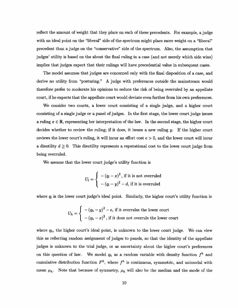
as shown in Figure 1. Notice that the probability of review decreases in c, as expected.
Figure 1 shows that the variance in this case is minimized at c m 2.3, which corresponds to
a likelihood of review of around 10%. At this level, the variance of the final outcome is 0.52.
When both courts have the same variance, uniformity is optimized at a relatively low likelihood
Figure 1: Variance and Probability of Reviewas Functions of c, One-Judge Appeals Court
Latitude (c)
Figure 1-1:

Figure 2: Variance and Probability of Review as Functions of c, Three-Judge Appeals Court
eUS
w
Laeitude (c)
Figure 1-2:
of review.
Next, we consider the effect of using 3-judge panels in the higher court, so that a2 - 1
Figure 2 shows the impact of c on the variance of the outcome and the probability of review.
Here, the minimum variance is approximately 0.17 at c ? 1.1; the probability of review is
approximately 0.34. At this level, the variance is reduced by a factor of almost 6. Since the
probability of review is 0.34, and each appeal requires 3 judges, the court system will require
the same level of resources ("judge-hours") on the higher court as on the lower court.
The degree of latitude is not directly controlled; it is determined in equilibrium by the
marginal effort cost of the higher court judges. Suppose, for example, that there are equal
numbers of judges on both courts, and that each case on the higher court requires a panel
of three judges. In equilibrium, if each higher court judge is participating in as many cases
as each lower court judge, then the probability of review must be ½. This would mean that
c 0 1.1, which is close to the optimum.
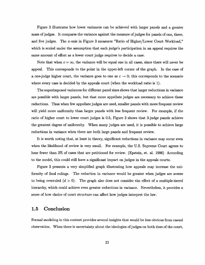
Figure 3 illustrates how lower variances can be achieved with larger panels and a greater
mass of judges. It compares the variance against the measure of judges for panels of one, three,
and five judges. The x-axis in Figure 3 measures "Ratio of Higher/Lower Court Workload,"
which is scaled under the assumption that each judge's participation in an appeal requires the
same amount of effort as a lower court judge requires to decide a case.
Note that when c = oo, the variance will be equal one in all cases, since there will never be
appeal. This corresponds to the point in the upper-left corner of the graph. In the case of
a one-judge higher court, the variance goes to one as c -+ 0; this corresponds to the scenario
where every case is decided by the appeals court (when the workload ratio is 1).
The superimposed variances for different panel sizes shows that larger reductions in variance
are possible with larger panels, but that more appellate judges are necessary to achieve these
reductions. Thus when few appellate judges are used, smaller panels with more frequent review
will yield more uniformity than larger panels with less frequent review. For example, if the
ratio of higher court to lower court judges is 0.5, Figure 3 shows that 3-judge panels achieve
the greatest degree of uniformity. When many judges are used, it is possible to achieve large
reductions in variance when there are both large panels and frequent review.
It is worth noting that, at least in theory, significant reductions in variance may occur even
when the likelihood of review is very small. For example, the U.S. Supreme Court agrees to
hear fewer than 3% of cases that are petitioned for review. (Epstein, et. al. 1996) According
to the model, this could still have a significant impact on judges in the appeals courts.
Figure 3 presents a very simplified graph illustrating how appeals may increase the uni-
formity of final rulings. The reduction in variance would be greater when judges are averse
to being overruled (d > 0). The graph also does not consider the effect of a multiple-tiered
hierarchy, which could achieve even greater reductions in variance. Nevertheless, it provides a
sense of how choice of court structure can affect how judges interpret the law.
1.5 Conclusion
Formal modeling in this context provides several insights that would be less obvious from casual
observation. When there is uncertainty about the ideologies of judges on both tiers of the court,

Figure 3: Variance ofFinal Rulings, by Panel Size
Figure 1-3:

then the strategic interaction between the lower court and the higher court can result in greater
consistency of interpretation that either court could achieve independently. Thus, even when
the higher court is much more consistent, it is still optimal to limit review to some degree.
In the legal literature, it is often assumed that more frequent review enhances predictability
in the interpretation of the law by providing closer monitoring of lower court judges and resolv-
ing conflicts arising from different cases. This assumption neglects the fact that higher court
itself introduces some uncertainty. For example, while the Supreme Court has been criticized
for not reviewing enough cases, commentators have also complained of doctrinal incoherence in
areas of the law in which the Supreme Court has been active. (Hellman 1996)
Similarly, questions of panel size are typically framed as a trade-off between consistency and
the use of judicial resources. As the model shows, however, using panels to increase consistency
in appellate courts may be counterproductive if it weakens incentives for moderation in the lower
court. Whether this effect is observable in practice is a question for future empirical research.
There are several theoretical questions arising from this model that could be explored in
future research. The model could be extended to consider multiple-tiered hierarchies, which
could potentially provide strong incentives for restraint in the lower court, while minimizing
concentration of authority in the highest court. A model that endogenizes the role of precedent
could help explain how appeals judges select cases for review, and also explore how the structure
of courts affects the evolution of precedent.
1.6 Appendix
Proof of Theorem 1:
First, note that for a given ruling x, the higher court judge has utility - (qh - x) 2 if he does
not review the case, and utility - (qh - y) 2 - e if he does review. Clearly, this latter term is
minimized at y = qh, so the judge will review the case if -e > - (qh - x) 2 . Hence the ruling
will be reviewed if Ix - qhl > =F = c.

Now for a given ruling x, the lower court judge's utility will be
Uz =
EUIx-c
S - (q--00
- (q, - qh)2, if the case is reviewed
- (q, - )2 , if the case is not reviewed
x+c
ql) 2 fh (qh) dqh + -(x- q) 2 fh (qh) dqh
+ - (qhz+c
Applying Leibnitz's Rule,
-(x-ql -c) 2 f h ( - c ) - 2 ( x - q ) [Fh (x+c)- Fh(x - c )]
- (X - qj) 2 [fh (X +C) - fh (X - c)] + (x - qj + c)2fh (X + C)= 2(x-q), [c[fh(x+c)+fh(X-c) - [Fh(x+c)
+ (c2 + d) [fh (x + c)- fh (x - C)]
Hence the first-order condition yields
(c2 +d) [,ch (II±+) fh (x-C)1x = qI 2 c [fh (x + c) + fh (x - c)] - [Fh (x + c) - Fh (x - c)]
To simplify our notation, let
1 (c2+d) [fh(+ ) - h ( - )]2 c [fh (x + c) + fh (x - c)] - [Fh (x + c) - Fh (x - c)]
n (x) = (c2 +d) [fh(X+C)_ fh (x - c)] , and
d(x)= c [fh(x+c)+fh (x c)] [Fh(x+c)-Fh (X- c)] .
Thus,
aEUIax
- Fh (~- c)]]

so that
n(x)qi = g(x) = d(z )
Proof of Theorem 2:
Let n(x) and d(x) denote the numerator and denominator, respectively, of g(x)
n (x) = (c2 + d) [fh(+) fh(- c) , and
d(x) = c[fh( + c)+fh(xc)] - [Fh(X +) - F h( )]
so thatn(x)q = g(x) = +()d(x)
Then g(x), n(x), and d(x) satisfy the following properties:
a) n(x) > 0 for x < Phb) n(x) < 0 for x > Ph
c) d(Ah) < 0
d) 0g(Lh) = PhFirst, we will show that n(x) > 0 for x <- Ph:
For x < IPh - c, the result follows from the fact that fh is increasing on (-oo, •h). For
P h - C < x < /Ph, note that
n(x) = (c2+d) fh(x+c) fh(x- c)]
S ( 2 +d) [fh(2g c ) fh (x-)]
> 0, sincex-c< 2,h-x-c< Ph.
Similarly, we can show that n(x) < 0 for x > I h. This also implies that n(Ph) = 0.
Now we show that d(Ah) < 0 :
Note that fh((Ph - c) = fh((Ph + c), and fh is increasing on (Ph - c, I'h) and decreasing on
(Ph, iPh + c). Thus fh(x) 2 fh(Ph - c) for all x E (Ph - c, /Ph + c), with strict inequality in a

neighborhood of Ph. Hence,
d(Ph) = f (Ph + c)+ f h( - hc) - [F"(, + c)- Fh (Ph- c)dh+c
11h -cc (. -c)+ f (pa -e) - f*(i)dtPh-CP1h+CJ [f (P - c) - f (t)] dt
Ah-C< 0.
Also, this implies that n(h) - 0 so that g(Lh) = ph"d(Pih) --
Now d must be negative over the range of x. If d(xi) = 0 for some value xz > Ph, then g
will asymptote to +oo at xl. Similarly, g will asymptote to -oo if d(xo) = 0 for some value
xo > Ph. Hence for all x for which g(x) is defined, d(x) < 0.
Since n(x) < 0 for x > uh and d(x) < 0, it follows that g(x) > x, and therefore, Ph < x < q1.
Similarly, for x < Uh, we have q1 < x < Ph. Therefore the judge chooses a ruling x between qi
and Ph.
Proof of Theorem 3:
We will show that g has asymptotes on both sides of PUh. First, note that
J d(x)dx = fc ["(X + c) + f h(x - c)] dx - f (t)dd--00 -00 -00 X-C
2c- 2c 2 fh(t)dt
-- 00
=0
Since d is continuous, there exists some xo such that d(xo) = 0.
Also, Xo ~ Ph, since d(ph) < 0, as shown in theorem 2. If there exist multiple choices
for xo, choose the value that minimizes 11th - XoI. Since f is symmetric about Ph, it follows
that d is symmetric about Ph, so that d(xi) = 0, where X1 = 2 ph - xo. For simplicity, we
can assume that xo < Ph < xl. Now n(xi) < 0 and n(xo) > 0, so lim_,o+ ( = -oo and
lim- (x = +oo. Thus g has asymptotes at xo and xl and has a range covering the entire
real line on (xo, xl). Since qj = g(x), it follows that xo < x < xl. Thus the lower court's
choice of ruling will always be bounded by the interval (xo, x1 ).
Proof of Theorem 4:
Consider any value yo. Then Fy (Yo) = Pr (y < yo). Now there are two conditions on qj
and qh that will achieve y < yo: either x < yo and the case is not reviewed or y < yo and the
case is reviewed. Thus
Pr (y < yo) = Pr (qh < yo and Ig- (q) -qhl > c)+ Pr (g-1 (q) < yo and g- 1 (qI) - qh < c)
We may sum the two probabilities on the right-hand side because the events are disjoint. We
consider each of these terms separately.
Pr (qh < YO and g-(ql) - qh > c) = Pr(qh < yo and (qI) ' [qh - c, qh + c])yo
1 - F[ (g (qh + c)) + F (g (qh - c))] fh (qh) dqh-00

g-~ (q) < yoand g- 1 (qi) - qhl • c
= Pr (q, < g (yo) and (q) E [qh - c, qh + c])
yo+c min{g(yo),g(qh+c)}
-I (-oo g(qh-c)
fh (qh) f' (qi) dqjdqh
yo-c g(qh +c)
I I f (qh) f (q) dqldqh-00 g(qh-c)
yo+C g(yo),
yo-C g(qh-c)
yo-cJ [F' (g (qh-00
fh (qh) fl (q1) dqjdqh
+ c)) - F1(g (qh -
yo+c
+ [JF (g (yo)) - F' (g (qh- c))] f (q) dq
Y0-C
Hence
- F' (g (qh + c)) + F1 (g (qh - c))] fh (qh) dqh
+ [F' (g(qh+c)) - F1 (g (qh -C)) fh(qh) dqh
yo+c
+ F (g (yo)) - F' (g (q - c))] fh () dqh
yo-c
By Leibnitz's Rule,
And
Pr (
FY (yo) 1Yo-
c))] fh (qh) dqh

f" (y) = [1-Fl(g(y+ c))+Fl(g(y-c))]fh(y)
y+c
+ f l(g (y)) g' (y) fh (qh) dqhy-c
= [1-F(g(y+c))+Fl(g(y-c))] fh(y)
+ [Fh (y + c) - Fh (y - c)] f (g (y)) g' (y)
Lemma 9 There exists xo such that d(xo) = 0.
Proof.
d(x)dx-00
00 00 X+C
Sc [( + c) + f(x - c) dx - f ()d-00 -00 X-C
00
= 2c- 2c / fh(t)dt
-00
=0
Since d is continuous, there must be some x0 for which d(xo) = 0. m
Lemma 10 If fh is convex on the interval (x - c, x + c), then d(x) > O. Similarly, if fh is
concave on the interval (x - c, x + c), then d(x) < 0
Proof.
d(x) [f h(x + c) + f (x - c)] - f (t) dX--C
x+c
z-C l-l+c 1-x+cf h( x - c) + - fh (x + c) - f(t) dt2c 2c
x+c
Sx- t+c C (x - c) + h( + c) -2c 2cX-C
> 0
xt-t+ec t-x:+ cfh x t+c(x -c) C+ (x + c) dt2c 2c

Lemma 11
(C2 2cA) 0 (A) + (C2 - cA) (-)a 01 and
(cA + c2 + 0,2) 0 A~ ) + (CA - C2 - U2)0 (-C[ (A + c)2 + oA] (A±) + [(A - C)2 - uA] 2 (A•)
(cA + c2 + c 2) (A) + (cA - C2 - U2) (A-)
Proof.
jA+c)acc A+c
a(A -c
-4
Differentiating yields
+c ' (A) ( + 1)
01[ 0( a
Rearranging terms and substituting for 0' yields
dA (c2 + ) ( )dc (cA + c2 + 2) ( )
We similarly differentiate with repsect to a:
c A+c IdA A+ca 0- [a do a92
c, A-c I1dA A-c]0 a a do e2- A+c[1 dA A+c
0- ) a da 92
(A-_ c IjdA A-c]a )[a d a 2 a
Rearranging terms yields
(A + )2 +A (A+) + [-L ( C- C2_ (~-c)
(cA + C2 + 2)( +c) + (cA -C 2 - U2) A-c
( A+c01
dAda
I• (A-c) (d 1
+ (2 - ) ()+ (A -C2 - 2)0 (, )
A c c
A c
Proof of Theorem 5:
Part (a):
We construct Taylor series for (D and 4 around A:
c (A+ c)
(A+c)
A c
+ A -A-c
-# -
2c0-4
2c= -40o
(A)a(A)
(A)+C)+ 0 (c4)
+ 3 30 (Aa
+o 0(c4 )
If A satisfies Equation (*) for sufficiently small c, it follows that 4" (A) = 0, or equivalently,
[1 ( ) =0 =
Part (b):
dAlimc--*o dc
=limc--*O
= lim
(c2 + cA) (c) + (c2 - cA) c (\)
(cA + c2 + U2) (+) + (cA - C2 - 2) (A-c)
A [0 (ý+-c))A ~ ~ + ý---c + 1-2 [0 (A> c ) >
2A4 (a) + U 24' (a)
Part (c):
=limC-+OO
=limC--+00
(cA2 + c2) (Ac) + (C2 - CA) (Ac)
(cA + c2 + 0-2) (A) + (CA -C2 - -c2
(c + A) ±+ (c - A)
-2c,
(c + A) e + (c - A)= lim -2cA
C- *o (A c)e -- +(A -c)
Note that we cannot have A - 0 as c -+ oc; if this were true, then 2 () - 1 as c --+ oc,
dAlim
c-*oo dc
A+c+ 0' + (A-c-
which is impossible.-2cA
Hence e - -+ 0 as c --+ oo, so
Part (d):
From Lemma 11,
(c2 + cA) 0 ( ) + (c2 - cA) (A)(cA + c2 2 ) ( ) + (CA - C2 - a2 )(
C2 (cA\) tanhC
+ 1 tanh -(, )
First, we consider the case where a = 1, so that
dA c2 - (cA) tanh cAdc (c2 + 1) tanh cA - (cA)
From part (a), we know that A -- 1 as c -- 0. Substituting the power series of tanh into
(1.1) yieldsdA c2(1 - A2) 2+ c4A 4 + O(c 6 )dc c3 (A - A3)+ O(c)1-( , ) + o(•)
so that as c -- 0, -- 0 and - . Thus A is increasing in c when c is sufficiently close to
zero.
Now consider the curve S defined by the equation
c2 - (cA) tanh cA = 0
Implicitly differentiating (1.2) yields
dA 1 - c2 sech2 cAdc tanh cA + cA sech 2 cA
so S has strictly positive slope. Note that S contains the point (c, A) = (0, 1), since A - 1
as c -- 0 in equation (1.2). Also, as can be seen in equation (1.3), S has infinite slope at
dAlim -
c--oo decA-c
- = 1.
(1.1)
(1.2)
(1.3)

(0, 1). Thus, for sufficiently small values of c, the solution to (1.1) must lie between the x-axis
and curve S. If the solution to (1.1) intersected S at another point, it must approach S from
below, and hence have positive slope at that point. However, the solution to (1.1) must have
zero slope at any point at which it intersects S. Therefore the solution to (1.1) will always be
between the x-axis and curve S.
In the region between the x-axis and curve S, the numerator [c2 - (cA) tanh cA] in (1.1) will
be strictly positive, and the denominator will be postive for all c, A > 0. Hence is strictly
positive, so A is strictly increasing in c.
The general case, when a $ 1, now follows easily. Let = , = , and U = 1. By the
above reasoning, - is strictly increasing, hence A is strictly increasing.
Lemma 12 As c - 0, g(x) x-+x + ,2 and the density function of x approaches
1 +) exp . _2).
Proof. We use the Taylor Series expansions for Fh(x) = 4c (1) and fh(x) = (Z),
substituting them into the formula for g(x). This yields
a -2c 2. + O(c2) 3 a2xg(X) = x + ( x +
2x2 2c22 -1)+O(c4) 2 2 - 2
Now ql = h (x), so as c -- 0,
fx(x) = fl(g(x))g'(x)
3 a 2 3 ,2 (U2 + X22 a 2 - T2 2 ( 2 - X 2 ) 2
1 (1a 3 ( 2 (g 2 X 2)) exp 1X2(1+ 3 a2)2
-7 2 (02 - X2)2 2 2 u2 - X2
Lemma 13 As c - 0, fx(x) will have a single peak at x = 0.
Proof. First, assume a 2 = 1, so that
fX(x) = 1 + X2) exp -X2 (1+ 1 )22 (1 - 22342 2 21
34

2
and let s -= -2. Since x is defined on [-1, 1], s will be defined on [1, oc]. Substituting s into
the above equation,
log f x (x) =-log o + log + 3s(2s-1) - 1- 1 + S2
Taking derivatives yields
& 12s-3 1 1 (9 \ 9log fxx) =X+ 3 --- (+ 'sOs 6s2 - 3s + 2 2 s2 4 2
and
(2 6 +9(s-2s2) + 1 9log f (x) = )2as (6S2 - 3s + 2)2 T3 26 - v2 + 9(-1) [- sinces>< 4( + 12 - , since s > I(6S2 - 3s + 2)2
(6s2 - 3s + 2) 2 1 2< 0
Thus o log fx(x) will be negative everywhere if - log fx(x) < 0 at s = 1. Now
O 9 25alog fX(x) 9 25 0Os s=1 5 8
which provides the desired result. Also, as>0 x > 0, so> logfx(x)<0 x>0. Thus
fx(x) is decreasing for x > 0 and increasing for x < 0. Therefore fx has a single peak at x = 0
when a 2 = 1.
Now for o-2 $ 1, we normalize the other parameters. Let 'E= , ~ = , and i = 1. Using
the above reasoning, the density function of i must have a single peak at Y = 0. Since x = aT,
it follows that the density of x must also have a single peak at x = 0. *The above results describe the shape of fx, the density function of the lower court's ruling,
as c -- 0. For sufficiently large values of a, fx is single-peaked and symmetric around 0, and
bounded at ±a. It follows, and we state without proof, that the variance of x must be strictly
less than o. This means that as c -+ 0, the lower court's rulings will have lower variance than

the higher court's, irrespective of the distribution of both courts' preferences. However, as
c -+ 0, the likelihood that the lower court's ruling will stand approaches 0. For very small c,
the second effect dominates, so that a slight increase in c will reduce the variance of the final
ruling. This provides intuition for the following result.
Proof of Theorem 6:
When c = 0, every case will be appealed, so the final ruling will be the appeals court's
preference point. Thus the distribution of the final ruling will be the same as the distribution
of the appeals court's preferences, in this case, a normal distribution with mean 0 and variance
02. Now consider e > 0. Let vo = a 2 be the variance of the final ruling when c = 0, and ve
be the variance when c = e. Then the final ruling will be the same in both these cases unless
Ix - qhl < e. Thus
oo qh+E
vo-V = (q -)x(x) (I-) dxdqh-oo qh--
00 qh+C
1 Jeqf(1hŽ.) f (q2_X 2) fx(x)dxdqh-00 qh -E
positive
Note that the second integral is positive, because
qh+e eJ (q x) fx(x)dzX= - (q + t)2 ]f th+t)+2qh-E 0
= {[-2qht - t2] f (qh + t)dt + [2qht - f(qh - ) dt0
= 2qt[f(qh - t) - fx(qh + t)Jdt + --t 2 [fx(qh - t) + fx(qh + t)]dt
0 0
postive, 0(e 2 ) negative, O(E3 )
so it follows that the entire double integral is positive. Therefore vo > ve for small e.
Proof of Theorem 7:

Part (a): Let = and a= . Then c +- =-Now as a -,O c o -- co. From Theorem 5, - I as E - o, hence v 1. ThusN 1 as a ---. 01 c C
lim•-o A(c, a) = c.
Part (b): As above, let = Xand = -, so that c (A+ c~) (A-)]= ( •-C, [0 tha + a- =) + 0-
- . In this case, we have-- 0 as a - oo. ThusA -+ 1, so - 1 as a -- o. Hence
lim doo = _1.
Part (c): First, we must show that lim,, 0 c = -oo. Since c) +
S(A+) - 4 (-), it follows that (A-c) < 1. Thus -½ (A-c)2 < log v-c I >log Note that > log is impossible for large enough a, since 0() will then be
convex on (X, ) . Hence, A < - log 2 .-- Thus, as a -+ 0, - - o.
Now,
. = [(A + c)2 A (A)+ A C)2lim =lim0-0o do o->o (cA + c2 + 2) ( c) + (A - C2 _ ,2) (
-2cA(A + C2 + 0 -2 e •-
+ (CA - C)2 - 2
Slim -2cA0'-0 ( 2 + • + 2)e2 (A 2 _ ,2)
[c ( A-)2 A]X--clim
= limA =-oo.a--*O
Proof of Theorem 8:
The bounds of rulings will be invariant to d because they are determined by where the
denominator of g(x) crosses the x-axis. Since d does not appear in the denominator of g(x), it
will not affect the bounds of rulings.
To show that the variance of x is decreasing in d, note that
1 ( c2 +d) [ ) x-c.-X) = -+ 2 (aa)]20• c [ (x[• c) + q (v)] - [4 (O) - D (' )].
By theorem 2, the fractional part above will be positive when x > 0 and negative when x < 0.
Thus ax is strictly increasing in d, and therefore -•, is strictly decreasing in d. Since

x = g -(ql), this means that a larger d results in lower variance of x.

Chapter 2
Collegial Decision Making in the
Courts of Appeals: An Empirical
Analysis
This chapter studies the interaction between ideology and collegiality in the U.S. Courts of
Appeals. In a collegial court, a ruling issued by a three-judge panel is typically the product
of a collaborative effort by all of the judges. Although cases are formally decided by majority
vote, it is commonly understood that judges favor unanimity in their rulings, so that judges
with different viewpoints will often negotiate to reach a compromise.
Thus, in a collegial court, judges' observed votes are not necessarily reflective of their true
preferences. This presents a significant challenge for any empirical study of judicial decision
making. In addition, decisions in different cases are not comparable, and the merits of each
case are not readily observable.' For instance, if a judge votes in favor of a liberal outcome,
there are three possible explanations for the vote: that the judge is liberal, that the judge's vote
was influenced by liberal colleagues on the panel, or that the merits of the case necessitated
a liberal outcome. Only by examining many rulings, with repeated interactions over random
triples of judges, can we disentangle these effects.
1Although judicial opinions are published, and could theoretically be evaluated on some basis, these onlyreflect ex post justification by the majority; the legal merits and quality of briefing are still unobservable in thedata.
The goal of this paper is to analyze how the ideological preferences of judges translate
into observed votes. The paper develops a model of panel decision making and uses this
model to simultaneously estimate judges' ideological inclinations and the parameters of panel
decision making. These parameters can be interpreted as measurements of judges' willingness
to compromise, thereby providing measures of an important aspect of judicial collegiality. We
then apply this model to a data set of sex discrimination cases.
A second benefit of the model is that by identifying the effects of panel decision making, it
can estimate individual judges' ideological preferences based on their observed votes. This is
important for any empirical research that seeks to understand the motivations of judges - for
instance, how they are influenced by precedent or the possibility of appellate review, or how
their backgrounds affect their philosophies.
A willingness to compromise is one indication that the judges in a court maintain a norm of
collegiality. Judges who view their duty to interpret the law as a common objective - rather
than a means of achieving political goals - will strive to reach consensus in their opinions.
While some dissent can be healthy, too much public disagreement among judges can undermine
the prestige of the judiciary and the legitimacy of the courts.
A collegial environment may also have a positive effect on judicial rulings. Judges who are
open to opposing viewpoints will be more able to recognize the weaknesses of their own positions
and will therefore be able to produce opinions that can better withstand scrutiny. An opinion
that can garner the approval of all three judges on a panel is less likely to be controversial
than an opinion that produced by a 2-judge majority. The deliberative process may lead to
greater moderation: the minority judge can negotiate for the removal or revision of controversial
passages as a condition for joining the opinion. On the other hand, it is also conceivable that
compromise would result in narrow rulings that dispose of the case at hand without establishing
a workable precedent. Over time, such opinions could diminish the coherence of case law.
There has been recent interest in panel decision making in the academic literature, partly as
a result of debate between empirical scholars who have emphasized the ideological component
of judging, e.g., Sunstein, Schkade, and Ellman (2004), Revesz (1997), Tiller and Cross (1998,
1999a, 1999b), and judges themselves, e.g., Edwards (2003), Wald (1999), who downplay the
importance of ideology and emphasize collegiality in decision making. Previous empirical

studies, however, have relied on variables such as race, gender, and party affiliation, as proxies
for judicial ideology. For example, Sunstein, Schkade, and Ellman (2004) use the party of
the appointing president to examine ideological voting and "panel effects" across various areas
of law, and Tiller and Cross (1998) and Revesz (1997) do the same for challenges to EPA
regulations in the D.C. Circuit. Farhang and Wawro (2004) use race, gender, and Poole common
space scores (McCarty and Poole 1995) of appointing presidents and home-state senators to
study panel decision making in emplyment discrimination cases, while Peresie (2005) adds
additional variables for judges' prior experience to study the effect of female judges on panel
rulings in sex discrimination cases.
These variables are valid predictors under many circumstances, and have been used to
identify the presence of "panel effects," when judges' votes are affected by the other judges on
a panel. (Sunstein, et. al. 2004) However, the imprecision and limited variation of these proxy
variables make them poor candidates for developing a richer model of panel decision making
or determining the impact of intrapanel interactions on case outcomes. For example, several
papers have observed that unified panels are more likely to issue extreme rulings than mixed
panels, and have attributed this effect to the moderating effect of the minority judge on a mixed
panel. (Sunstein, et. al. 2004, Tiller and Cross 1998) However, these results are also consistent
with unobserved heterogeneity among judges appointed by presidents of the same party. In the
presence of unobserved heterogeneity, the median judge on a panel of three Republicans should
be more conservative, in expectation, than the median judge on a panel with two Republicans
and one Democrat. Without a richer model, it is impossible to distinguish the moderating
effects of a minority judge from the effects of within-party heterogeneity.
Instead of relying on proxy variables, this paper uses a structural model to estimate judges'
ideological inclinations, or "attitudes" (Segal and Spaeth 2002), in a one-dimensional spectrum
based on their actual votes. The model uses a judicial negotiation game with flexible parameters
to predict observed votes based on judicial inclinations, and then estimates both the parameters
of the game and the inclinations of individual judges using maximum likelihood estimation.
The estimation procedure controls for the incomparability of cases by treating the merits of
each case as a random effect and exploiting the exogenous variation resulting from the random
assignment of judges to panels. By eliminating the problem of proxy error, the model can

provide more precise estimates of judicial ideology and better explore the dynamics of panel
decision making.
The spatial estimates derived from this model are significant because they can enable em-
pirical research on judicial decision making in situations where subtle influences on judicial
decision making might otherwise be obscured by "panel effects" and the imprecision of proxy
variables. This is especially important in situations where proxy variables are poor predictors2
and where there is insufficient variation in these variables3 . Moreover, by providing numerical
estimates of the parameters of panel decision making, this model can analyze the impact of
collegial decision making on case outcomes and has the potential to compare collegiality across
judicial circuits, time periods, and areas of law.
Another advantage of the structural approach is that it can generate out-of-sample predic-
tions. For example, it could predict the effect on case outcomes in a particular circuit if a
liberal judge were replaced by a conservative, or after several more years of Bush appointees.
It could also potentially evaluate the impact of court reorganization plans, such as proposals
to split the Ninth Circuit.
The primary assumptions underlying the model are that judges have preferences over ideol-
ogy, and that they prefer unanimous rulings. These assumptions are relatively uncontroversial.
While there has been much debate about the importance of ideology in judicial decision making,
few would deny that it plays some role. Several empirical studies have found judicial ideology
to be a significant factor in case outcomes. (Sunstein, Schkade, and Ellman 2004, Revesz 1997,
Tiller and Cross 1998) Even several federal judges, who have argued against the importance
of ideology in judicial decision making, concede that it is still a factor in some cases. (Edwards
2003, Wald 1999)
It is also widely accepted that judges strive to reach unanimity in their decisions. A dissent-
ing opinion weakens the legitimacy of the panel's ruling, and frequent dissents can diminish the
authority of the court. Dissenting opinions require significant effort on the part of the minority
2 For example, Sisk & Heise (2005) find that party affiliation has no predictive value for judges' votes inreligious freedom cases, although they find that other demographic variables are significant. In state courts,foreign courts, and earlier periods in history, judicial appointments may be less partisan, and these variables maybe poor indicators.
3This is especially true in some state courts, where one party has dominated appointments. For example, inmost southern states for the century after Reconstruction, there would be little or no variation among judges inrace, gender, or party of appointment.

judge, and are also potentially costly to the majority, by increasing the likelihood that the
ruling will be overturned by a higher court or a non-judicial entity. (Daughety and Reinganum
2002) The "cost" of dissent also reflects the "danger of crying wolf too often": issuing too many
dissents may diminish their signaling value. (Ginsburg 1990) These intuitions have also been
confirmed by judges themselves, who have described consensus as a goal of panel deliberation.
(Edwards 2003, Coffin 1994)
The paper is organized as follows. Section I constructs a model of negotiation within
appellate panels, where judges have ideological preferences and prefer unanimity. This model
allows judges to vote against their ideological inclination when they derive a greater benefit
from consensus. Section II discusses the technique for estimating the parameters of the model.
Section III describes the data set. Section IV discusses the estimation results for the judges
and for the parameters governing the dynamics of panel decision making. Section V uses
the model and the estimated parameters to make out-of-sample predictions. The first part
of Section V estimates how often a unanimous decision results from actual agreement among
the judges, as opposed to judicial compromise, and how often the majority position dominates
when compromise occurs. The second part compares the distribution of outcomes when cases
are decided by single judges and three-judge panels, to provide a sense of how panel decision
making moderates rulings.
2.1 Model
We model the panel deliberation process as a two-stage game, where judges have ideological
preferences on a one-dimensional spectrum and favor unanimous rulings. The merits of each
case can be represented as a point r on the real line, and the position of each judge participating
in the case will be represented by a point ai E R. Each judge may choose a ruling vi E {P, D},
representing a vote in favor of the plaintiff or defendant, respectively.4
We represent the ideological component of the judge's utility as (-1)'P (ai - j7), where Ip
is an indicator function such that Ip = 1 when vi = P. Thus, when ai > 77, the judge will
prefer to choose vi = P, and when ai < 0, the judge will choose vi = D. We can think of
4In cases at the appellate level, the term "plaintiff' will always denote the original plaintiff in the case.
a judges with greater ai as being more liberal, in the sense of being more sympathetic to sex
discrimination plaintiffs, and judges with lower ai as being more conservative. Cases with
greater 7 are stronger cases for the defendant while cases with lower 7r are stronger cases for
the plaintiff.
We model the preference for consensus by imposing a cost Cm on each of the majority
judges and a cost Cd on the dissenting judge when there is a dissent. Each judge's total utility
is therefore
Ui = (-1) (ai - 7) - Imcm - IdCd
where Im and Id are indicator variables for judge i being in the majority and the dissent,
respectively. When cases are unanimous, Im = Id = 0.
The judicial deliberation process is modeled as a full-information two-stage game. In the
first stage, the judges take an intial vote. If there is disagreement, the minority judge may
choose to change his vote in the second stage.5
When r7 < min{ail or max{ai} < 77, the decision will be unanimous: all of the judges
will have the same preference, and none of them will have an incentive to switch sides. The
following results focus on the case where there is ex ante disagreement. Let ad denote the
judge in the minority position, aml denote the median judge, and am2 denote the other judge
in the majority, so that ad < r7 < aml < am2 or ad > 77 > aml > am2.
The following propositions will describe the unique subgame perfect equilibrium.
Proposition 14 When there is disagreement in the first stage, the minority judge will switch
sides in the second stage if and only if lad - 7rl < E. When this condition is satisfied, the
majority judges will vote their true preferences in stage 1.
Proof. The minority judge's utility from switching will be - lad - 771, and the utility from
5 We model deliberation as a two-stage game and use subgame perfection as the equilibrium concept in order toavoid the multiplicity of equilibria that could obtain in a one-stage game. When the cost of dissent is sufficientlyhigh for both the majority and the dissent, then either unanimous outcome would be a Nash equilibrium. Ifall three judges voted in favor of the minority's position, then there would be no profitable deviation for themajority judges, since the cost of dissent would outweigh the ideological gain. This would also be true in acooperative framework.
The choice of a two-stage game and the assumption that cm • Cd eliminates the multiplicity of equilibria, thusallowing straightforward estimation of the parameters. When cm is close to 0, most of the indeterminate casesin a one-stage game result in a unanimous ruling in favor of the majority's position. As cm increases, a greaterproportion of these cases result in unanimous rulings in favor of the minority's position
not switching will be lad - 771 - Cd. Hence the minority judge will switch sides if and only if
lad - 771 < E. Since there will be unanimity in the final stage, the majority judges get utility
lam,i - 771 in the final stage if they vote their true preferences, so there is no profitable deviation
for them. m
Proposition 15 The judges in the majority will vote against their true preferences if and only
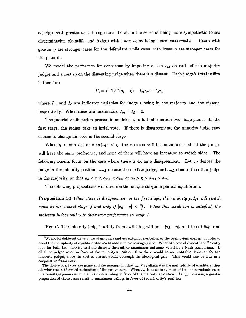
if lad - 71 > and laml - 71 < - and am2 -771 < a
Proof. First, suppose that lad - 7I > a and lami - 771 < c and lam2 - 771 < P. Then
by proposition 14, the minority judge will always vote his true preferences. If both majority
judges vote sincerely, the median judge will have utility laml - 771 - Cm, but if the median judge
votes against her ideological preference, then the other majority judge will switch sides in the
final stage, and the median judge will have utility - (aml - 771. Thus, there will be a unanimous
opinion in favor of the minority judge's preference when these conditions are satisfied.
If any of these conditions fail, then the majority judges will vote their ideological preferences.
If ad - r/I < E2, then proposition 14 shows that the minority judge will not dissent, and the
majority will not switch sides. When lami - 71 > m, the median judge would prefer a non-
unanimous opinion to switching sides. When lam2 - 771 > fL, the more extreme majority judge
would dissent if the median judge switched sides; there will be a dissenting opinion either way.
Thus, the median judge will vote her true preferences. m
Proposition 16 The judges in the majority will vote true preferences and the minority judge
will dissent if and only if lad - r71> Ed and either Iaml - 77 > = or lam2 - M7 >
Proof. If lad - 771 > and lam2 - 771 > E, then these two judges have an irreconcilable
disagreement, and one of them will dissent in either case. Since the median judge will incur
the cost Cm in either case, she will maximize her utility by voting in favor of her ideological
preference.
If lad - 771 > - and lami - 771 > -c, then the median judge gets utility lami - 771 - Cm from
voting in favor of her ideological preference, and a maximum utility of - laml - 771 if she joins
the minority judge. Thus voting her true preference will always be the dominant strategy. 0
These propositions describe the outcome of judicial deliberations. Proposition 14 provides
conditions for a "collegial concurrence" (Sunstein et. al. 2004): when the judge in the mi-
nority position does not feel too strongly, he will join the majority opinion. Proposition 15
demonstrates that it is possible, under certain conditions, to have "minority rule." In these
circumstances, a minority judge with strong ideological preferences will be able to induce a
relatively indifferent majority to switch sides. Proposition 16 provides conditions for when the
judges will not reach unanimity.
The following table summarizes the results of these propositions for judges with ai < aj <
ak :
Conditions for ai, a , ak, r : Outcome: (vi, vj, vk)
ai < aj < ak < 77 (P, P, P)
q < ai < aj < ak (D, D, D)
ai < aj < 7 < ak < rl + Cd (P, P, P)
77 - cd < ai < 77 < aj < ak (D, D, D)
ai < 77 -Cd and aj <77 - cm and ak > r +Cd (P, P, D)
ai < 77 - Cd and aj > 77 + cj and ak >7 + Cd (P, D, D)
77-cd < ai and 77 -cm < aj < 7 and ak > 7 + d (D, D, D)
ai < r - Cd and -77 < aj < r +cm and ak < 7 + Cm (P, P, P)
The following corollaries provide the conditions for independent voting and majority rule in
panels.
Corollary 17 When Cd = cm = 0, judges will vote purely on an ideological basis, and will not
be influenced by the other judges on the panel.
Proof. Propositions 14 and 15 provide conditions for when judges will change votes in
order to reach consensus. When Cd = cm = 0, these conditions cannot occur. Since judges
will never switch sides, their votes will be determined solely by their ideological preferences. 0
Corollary 18 When cm = 0, all case outcomes will be determined by majority rule.

Proof. By proposition 15, the majority will never vote against their true preferences, since
(ami - 771 > I = 0. Hence the majority's ideological preferences will determine the case
outcome. U
Corollary 17 shows that when Cd = Cm = 0, there will be no panel effects in the data: each
judge's vote will be independent of the characteristics of the other judges on the panel. All
cases will be decided by majority vote, and the proportion of unanimous rulings observed in
the data will reflect the actual degree of agreement among the judges.
When cm = 0 and Cd > 0, corollary 18 shows that the minority judge may still switch sides,
and we will therefore observe panel effects in the data, but case outcomes will be the same as
under independent voting. In this case, the proportion of unanimous rulings will overstate the
level of actual agreement among the judges.
2.2 Estimation
In this section, we describe how to estimate the parameters of the above model discussed in
section I. Consider a data set with n judges and T cases. Each case will be decided by a panel
of three judges, selected at random. We represent each judge by a parameter ai representing
judge i's position on an ideological spectrum, where a greater ai corresponds to a more liberal
judge.
Let St = {a, a2, a3} be the set of judges who participate in case t. We assume that each
judge's preference in case t is of the form ait = ai + eit, where ai is a judge fixed effect, and eit
are iid N(0, 1). This error term accounts for the fact that ai is not a perfect predictor of each
judge's approach to each case. Since the merits of the case 1t are not observable, we treat it
as a random effect, with 77t - N(0, a2), where a is a parameter to be estimated. This accounts
for the fact that the judges' attitudes toward a particular case may be highly correlated; in
many cases, liberals and conservatives will agree on the merits. The parameter a represents
the magnitude of the correlated component of the judges' preferences: a larger a (keeping all
other parameters constant) means that there will be more "easy cases" and consequently more
ex ante agreement.

Let yit be judge i's preference in case t. Then
Pr(yit = P) = Pr(ai + Eit > it)
We will estimate the parameters using maximum likelihood estimation. To derive the likelihood
for a unanimous ruling, recall that such a ruling can occur three ways: from ex ante agreement,
the minority switching sides, or the majority switching sides. The probability of a unanimous
"P" vote following from ex ante unanimity is
P(al -- ,t)((a2 -, qt),D(a3 - 77t)
By proposition 14, the probability of arriving at a unanimous "P" ruling after the minority
judge switches sides is
3
i=1j,kESt-{i}
We can derive the probability of the majority switching sides to reach a unanimous "P"
vote using proposition 15:3
i=1
where
+ [+ ( - T + --D(aj - 7t)] 1[ (aj -,t + )- ( -7t)]
- (a(k- 7t+ 2 ) -)(aj-t)] [4P(ck - T+ -+2 I(ak -qt)]

Hence
L((P, P, P) I t) =3
i,j,k
-2k(al - rt)4I(a2 -{it)}(a3 - 7t)
And similarly,
L((D, D, D) I t) =3
Z ý (-t + 77t + )(-'d) C -a, + 77)C-ck + 7t)i=1
j,kESt-{i}3
i=lj,kESt-{i}
-2M(-al + 7t)D(-Q 2 + 77t)4(-a3 + 7t)
To derive the likelihood function in the case where one judge dissents, we use the conditions
given in proposition 16:
L((P, P, D) I t) = (- Q-3 + 7 t - 1) [(Di - q t)(o2 - It) - ~I(al, a2)]
Since qt is unobserved, we must integrate over qt to get the unconditional likelihood:
L ((P, P, P)) = L((P, P, P) 1 71) d7
which can be estimated using Gauss-Hermite quadrature. The unconditional likelihoods for
the other cases can be derived in a similar fashion.
The parameters to be estimated are the judge fixed effects ai d, c, , and a. The maximum
of the log-likelihood function is estimated using Newton's method. Standard errors are derived

from the inverse Hessian matrix. All optimization routines were coded in Matlab.
2.3 Data
The data consists of 1080 sex discrimination and sexual harassment cases decided by three-judge
panels in the U.S. Courts of Appeals between 1995 and 2002. The data set was taken from a
larger data set collected and made available by the Chicago Judges Project of the University
of Chicago Law School.6
Because the model assumes that judicial preferences can be mapped onto a one-dimensional
spectrum, the data is limited to a single area of law. Sex discrimination cases were chosen for
several reasons. First, the laws governing sex discrimination cases have substantial ambiguities,
thus allowing judges substantial discretion in interpreting the law and providing for a role
for judicial ideology. Second, judges' attitudes toward sex discrimination law are plausibly
one-dimensional; although there are numerous subtleties in different areas of the law, it is
believable that judges' interpretations would be influenced by their attitudes toward workplace
discrimination, and whether they think the laws should be applied broadly or narrowly. Finally,
sex discrimination law is "moderately ideological," in the sense that there are likely to be
ideological differences among judges, but not so large as to overwhelm collegial effects.
For each case, the data set provides the identities and votes of the three judges. A case is
coded as "P" if the court provides any relief to the plaintiff; otherwise, it is coded as a "D."7
Plaintiffs won 41% of the cases, and 42% of the judges' individual votes. 92% of the cases were
decided unanimously, and about 3% of judges' votes are dissenting opinions.
There are 438 judges who appear at least once in the data, and the most appearances for an
single judge is 52. Because of the time period involved, the data are dominated by appointees of
Presidents Carter, Reagan, Bush I, and Clinton. The differences between the Democratic and
Republican appointees is immediately evident: Carter and Clinton appointees ruled in favor of
6The cases were gathered using a Lexis search of the terms "sex! discrimination" and "sex! harassment."(Sunstein et. al. 2004) One case was removed from the data because it was decided by only two judges afterthe death of the third judge.
Note that this method of coding overstates the degree of unanimity in the data. Some cases may be codedas (1,1,1) even though a judge may have dissented on some portion of the ruling.

AllVotes, by Appointhing Presilent
800
700
600
500
400
300
200
100
0
E"D" votes1O"P" votes
Eisenhower Kennedy Johnson Nixon Ford Carter Reagan Bush I Clinton Bush II
Figure 2-1:
plaintiffs 53% of the time, versus 35% of the time for Reagan and Bush I appointees. Figure 1
shows the number of votes in each direction, where judges are grouped by appointing president.
An examination of the dissenting votes provides an even starker contrast between Demo-
cratic and Republican appointees. Carter and Clinton appointees combined for 36 dissenting
opinions, of which 34 favored plaintiffs. On the other hand, Reagan and Bush I appointees
combined for 34 dissents, of which only 7 favored plaintiffs. Figure 2 shows the number of
dissents in each direction, by president.
Of the 438 judges who appear in the data, 210 judges participated in at least 5 cases; the rest
are grouped together by appointing president. There are 10 such judge groups, corresponding
to presidents Eisenhower through George W. Bush. Table 4 in the Appendix provides summary
statistics for the individual judges and groups.
Note that most judges voted in favor of plaintiffs between 30% and 60% of the time, but

D issenting Votes, by Appointing President
25
20
15
10
E
cEisenhower Kennedy Johnson Nixon Ford Carter Reagan Bush I Clinton Bush II
Figure 2-2:
S"D" dissentsDO"P" dissents I

there are also outliers. On the conservative side, Judge Demoss supported the plaintiff in
none of the 13 cases in which he participated, with 3 dissents, while on the liberal side, Judge
Pregerson supported the plaintiff all nine cases in which he participated, with one pro-plaintiff
dissent.
2.4 Results
2.4.1 Judge Preferences
The results for each judge and judge-group are shown in Table 4 in the Appendix. For each
judge, we report the fixed effect ai and pi, the unconditional probability that a judge would
vote in favor of the plaintiff in a case drawn at random, where
PA -fl(ozi)i r) (I) dr
We report standard errors and 90% confidence intervals for the pi's. Table 1 summarizes the
distribution of the fixed effects and unconditional probabilities for the individual judges.8
8This table only includes those judges who appear at least 10 times in the data. The judge-group fixed effectsare excluded.
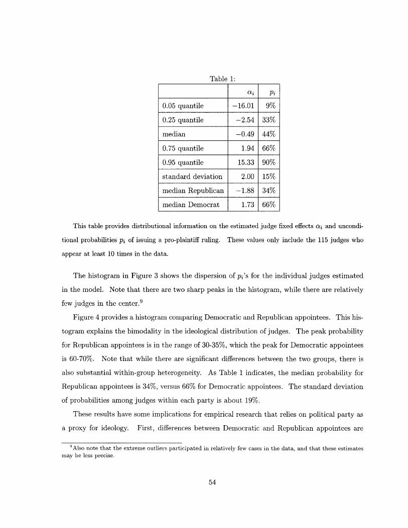
Table 1:
ai Pi
0.05 quantile -16.01 9%
0.25 quantile -2.54 33%
median -0.49 44%
0.75 quantile 1.94 66%
0.95 quantile 15.33 90%
standard deviation 2.00 15%
median Republican -1.88 34%
median Democrat 1.73 66%
This table provides distributional information on the estimated judge fixed effects ai and uncondi-
tional probabilities Pi of issuing a pro-plaintiff ruling. These values only include the 115 judges who
appear at least 10 times in the data.
The histogram in Figure 3 shows the dispersion of pi's for the individual judges estimated
in the model. Note that there are two sharp peaks in the histogram, while there are relatively
few judges in the center. 9
Figure 4 provides a histogram comparing Democratic and Republican appointees. This his-
togram explains the bimodality in the ideological distribution of judges. The peak probability
for Republican appointees is in the range of 30-35%, which the peak for Democratic appointees
is 60-70%. Note that while there are significant differences between the two groups, there is
also substantial within-group heterogeneity. As Table 1 indicates, the median probability for
Republican appointees is 34%, versus 66% for Democratic appointees. The standard deviation
of probabilities among judges within each party is about 19%.
These results have some implications for empirical research that relies on political party as
a proxy for ideology. First, differences between Democratic and Republican appointees are
'Also note that the extreme outliers participated in relatively few cases in the data, and that these estimatesmay be less precise.

Probability of Pro-Plaintiff Vote for Individual Judges
40
35
30
25
o 20
Z 15
10
5
0
o •' - 3 o 0o '0 7 po
Probabilit, in p
Figure 2-3:
.- I - IS' 00 d' 0 ' 0 d', 00
Srcente·rcent
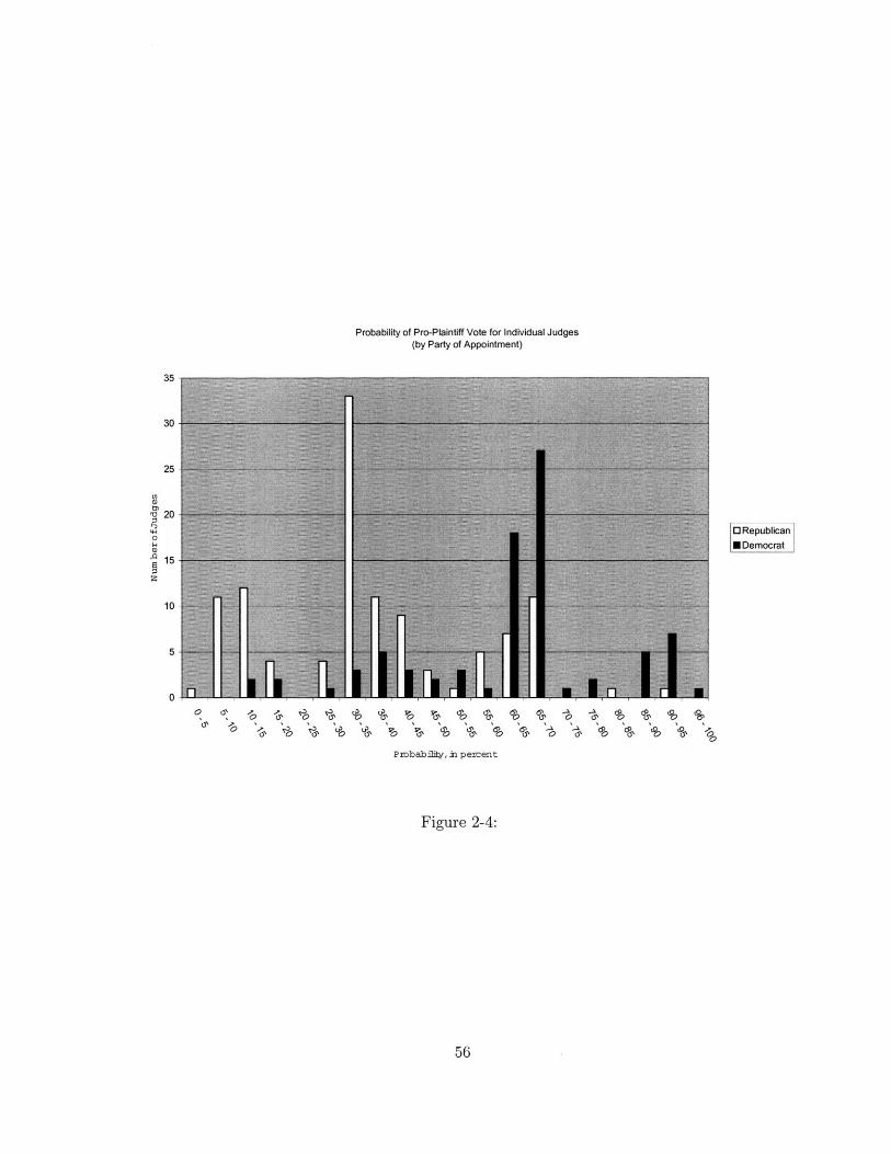
Probability of Pro-Plaintiff Vote for Individual Judges(by Party of Appointment)
35
30
25
S20
0
a15
10
5
0
Probability, in percent
Figure 2-4:
O Republican* Democrat
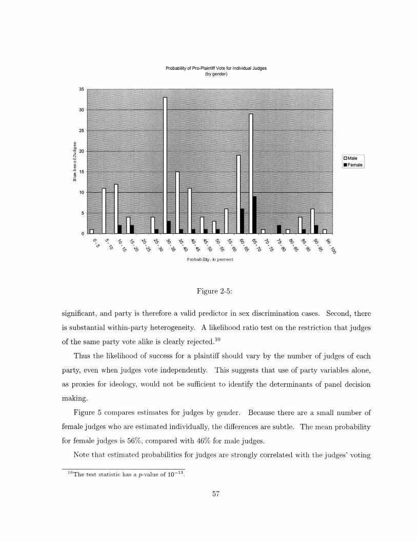
Probability of Pro-Plaintiff Vote for Individual Judges(by gender)
35
30
25
U)
1 20
0
15
5
0
E Male0 Female
o0 0 0 P & 3e 3o 01% u0 0 , , % O A 0 C' S ' so -
P•obability, in percent
Figure 2-5:
significant, and party is therefore a valid predictor in sex discrimination cases. Second, there
is substantial within-party heterogeneity. A likelihood ratio test on the restriction that judges
of the same party vote alike is clearly rejected. 10
Thus the likelihood of success for a plaintiff should vary by the number of judges of each
party, even when judges vote independently. This suggests that use of party variables alone,
as proxies for ideology, would not be sufficient to identify the determinants of panel decision
making.
Figure 5 compares estimates for judges by gender. Because there are a small number of
female judges who are estimated individually, the differences are subtle. The mean probability
for female judges is 56%, compared with 46% for male judges.
Note that estimated probabilities for judges are strongly correlated with the judges' voting
10The test statistic has a p-value of 10- 13

records, there are some substantial deviations. Since dissenting opinions provide strong evi-
dence of ideological differentiation from other judges on the panel, dissents will have an impact
on a judge's estimate. For example, Judges Rovner, Dennis, and Lipez are estimated to be
much more liberal than their voting records would suggest, because they each wrote multiple
pro-plaintiff dissents. Dissenting opinions by other judges on the panel also impact a judge's
estimate.
2.4.2 Costs of Disagreement
Table II provides estimates of Cd, Cm, and a:
Table 2:
estimate standard error
cad 6.28 0.94
cm 2.16 0.55
a 16.02 15.54
This table provides estimates of the "costs" of dissent, where Cd cost incurred by the dissenter and Cm is
the cost incurred by the majority. The variable a is the variance of the random effect associated with
each case. This represents magnitude of the importance of the legal merits of the case, compared to the
ideological component.
The estimates of Cd and cm represent the "cost" of disagreement. The higher these costs,
the more judges will be willing to compromise in order to achieve unanimity. Note that both Cd
and cm are positive and significant. Proposition 14 shows that outvoted judges are willing to
"travel" an distance of l = 3.14 in order to achieve a unanimous opinion. On the ideological
spectrum, this distance is a bit less than the distance between the median Republican and the
median Democrat (3.61). It is slightly greater than the distance from the median judge to
either the 0.25 quantile or the 0.75 quantile.
The parameter Cm is smaller but also statistically significant. A likelihood ratio test rejects

the restriction Cm = 0.11 Recall that cm = 0 corresponds to the case where the majority never
compromises, so that we can reject the possibility that outcomes are decided purely on the
basis of majority preferences. 12
We can also test for the presence of "panel effects." The restriction Cd = Cm = 0 corresponds
to the case where judges have no preference for unanimity, and therefore vote purely on an
ideological basis. A likelihood ratio test on this restriction clearly rejects 13 , so that we can
reject the hypothesis that judges vote independently. This confirms the conclusion made by
Sunstein, Schkade, and Ellman (2004) on the same data set using party data.
2.5 Simulations
One benefit of a structural model is that it lends itself to simulations and out-of-sample predic-
tions. In this section, we will explore a few applications. First, we will estimate the frequency
of compromise. We will use Monte Carlo simulation to estimate the proportion of unanimous
decisions that were the result of a compromise by one or more of the judges. Second, we will
estimate how appellate rulings would be different if they were decided by a single judge rather
than a three-judge panel. By simulating these results for the actual panels in the data, and also
for individual judges, we can get a sense of how panel decision making increases predictability
in rulings.
2.5.1 Frequency of Compromise
To understand the magnitude of "panel effects" we estimate the probability that one or two
judges would have switched votes in order to achieve unanimity. We estimate these probabilities
using Monte Carlo simulation, generating random values for r, and it jt, ~ Ekt for the actual
cases that occur in the data and including only those values that result in the observed vote.
Using these same parameters, we compare the judges' actual preferences to their observed votes.
The results are presented in the following table:
1 The test statistic has a p-value on the order of 10- 6 .12As we discuss in Section V, however, this effect is small in magnitude.13The test statistic has a p-value on the order of 10- 6 1.

Table 3:
Percent of Cases
ex ante unanimity 81.6%
one judge switched 9.3%
two judges switched 1.4%
dissent 7.7%
This table provides simulated estimates of the process by which panels achieved unanimous rul-
ings. These estimates are obtained by simulating judges' preferences in the data using the estimated
parameters, conditional on these simulated preferences resulting in the observed outcomes.
Several observations can be made from these results. First, there was ex ante unanimity in
a large majority of the cases. In 82% of cases, the judges' individual preferences all would have
led to the same outcome. This suggests that judicial ideology only plays a role in a relatively
small proportion of the cases.
Second, the judges are able to reach unanimity in about 60% of the cases in which there
was ex ante disagreement. Thus there would be more than twice as many dissenting opinions
if judges' votes were truly independent. Finally, the percentage of cases in which two judges
switch sides is tiny and insignificant. In most of these cases, the majority's position prevailed.
Although we have estimated some amount of minority influence, this result suggests that ma-
jority rule determines the outcome most of the time, at least in the context of sex discrimination
cases.
Third, the minority's position prevailed only in about 1.4% of cases. Note that this fre-
quency, though small, is statistically significant. However, since we only observe the outcomes
in the data, this may understate the influence of the minority judge. The minority judge may
have had a stronger influence on the content of the opinion, even if the outcome was unchanged.
These results also suggest that the outcome would only change in a small proportion of
cases if all appeals were decided by a single judge. Suppose that one judge were chosen from
the panel at random to decide the case. The probability that this judge would have ruled the

Case Outcome, Conditional on Legal Merits
0 01 02 03 04 05 06 07 08 0:9
Strength of Plaintiffs Case (quantile)
Figure 2-6:
same way as the panel is 81.6% + 2(9.3%) + !(1.4%) + 2(7.7%) = 93%. Thus, only in 7% of
cases would the outcome be different if decided by a single judge on the panel.
2.5.2 Individual Judge vs. Three-Judge Panels
In this section, we estimate the probability of success for the plaintiff for various levels of case
difficulty, based on the panel compositions that were actually observed in the data. This value
is the probability of a ruling favoring a plaintiff, using the parameters estimated in Section IV,
conditional on a given r1. We can also estimate the probability of each outcome if cases were
decided by a single judge. For simulated single-judge rulings, we weight the likelihood of a
judge being assigned by the number of times that judge occurred in the data. Figure 6 shows
the probability of the plaintiff winning the case, conditional on rq.
0.9
0.8
S0.7
Co•.)U)
(00>. 04
2 0.3
0.2
0.1
0
I I I I 2-.. -""
I
/I
//
--" C
I-
/
I/
//
/

The horizontal axis of Figure 6 measures the quantile of rl, the random effect, which repre-
sents the legal merits of the case. The point 0 on the x-axis represents the weakest case, and
the point 1 represents the strongest case. Note that the slope is increasing very sharply in the
center of the distribution. Thus there is only a small proportion of cases in the middle of the
distribution for which the outcome is truly unpredictable. On the other hand, there is only a
small proportion (about 10% of cases at either extreme) for which the outcome is completely
certain. 14
The dashed line in Figure 6 shows the probability of outcomes if the cases were decided by
a single judge chosen at random. Note that the outcomes are a bit less predictable under this
assumption. These results confirm the intuition that a panel of three judges will rule more
moderately and more predictably than a single judge.
2.6 Conclusion
Using a model to predict how judges' ideological inclinations will translate into observed votes,
this paper estimated judges' inclinations as well as the parameters governing panel decision
making in sex discrimination cases. The benefits of this method are that it can estimate how
both judicial ideology and panel collegiality affect votes and case outcomes. At least in the
context of sex discrimination cases, ideology and collegiality are clearly significant factors.
Although the results in this paper confirm the presence of panel effects, they cannot support
the claim that these effects have an impact on case outcomes. Rather, the panel effects seem
to result primarily from "collegial concurrences," when an outvoted judges joins the majority
opinion.
This conclusion is relevant to a proposal by Tiller and Cross (1999) to eliminate random
assignment in favor of a system that ensures diversity within each panel. If a judge in the
ideological minority exercises influence over the case outcome, such a proposal could result in
more moderate and uniform judicial rulings. On the other hand, if a "collegial concurrence"
has no impact on the case outcome, such a proposal would have little benefit.
One important caveat: the data only reveal case outcomes, and not the content of the
14Note that these results may be sensitive to the distributional assumption of the random effect.
opinions. The model in this paper therefore cannot capture how panel deliberations affect
opinion. Even if minority judges do not affect outcomes, in a directional sense, they may have
an impact of the degree of relief provided or the content of the judicial opinion. Since all of the
judges must sign on to a unanimous opinion, it is highly likely that judges do exert influence
over the content when they choose to join an opinion
The methodology used in this paper lends itself easily to other studies of judicial decision
making. This model could be used to compare the effects of collegiality in areas of law that
are more highly contested, as well as areas of law that are viewed as relatively nonideological.
This method could also be used to compare panel decision making by judicial circuit, to test
whether judges are less collegial in larger and more geographically dispersed circuits.

Chapter 3
Asymmetric Liability and Incentives
for Innovation
Firms' decisions to invest in product safety are influenced by both market and legal incentives.
A firm will save on liability costs if a product causes fewer accidents, and consumers will also
pay a premium for a safer product, but the size of this premium will depend on how well the
consumers are compensated for injuries under tort law. This paper explores the interaction
between product markets and product liability, and develops some insights on how the liability
system affects safety innovation.
Case studies and academic commentary have identified opposing effects of product liability
on innovation. Clearly, product liability may encourage firms to develop safer products in order
to reduce liability costs. On the other hand, liability may also lead firms to decide against
developing or releasing new products. (Viscusi 1991) National surveys have cited both effects
on firms' innovation decisions (e.g., Conference Board 1987, 1988). Viscusi and Moore (1993)
find empirical evidence that liability costs have a nonmonotonic effect on R & D intensity: low
levels of liability costs spur innovation, but high levels can have a stifling effect.
This paper develops a model that considers the distortions caused when liability does not
apply equally to all substitutes of a given product. If the alternative to purhasing a product
is purchasing no product, substituting the consumer's own labor supply, or buying from a
judgment-proof seller, then the product will be subject to stricter liability than its alternatives.

This may also be the case when a preexisting product has well-known risks that are not perceived
as design defects, but a new product with unfamiliar risks is subject to a higher standard. In
this case, the product will be competing against alternatives that have lower liability costs (but
also offer less protection) to consumers.
This "asymmetric liability" does not necessarily deter innovation. In fact, when the liability
system is efficiently administered, it may provide stronger incentives for the development of safer
products. When liability is efficient, higher liability costs translate directly into greater benefits
for consumers, and also provides greater differentiation between products. When liability is
inefficient, however, in the sense that liability costs exceed benefits to consumers, then goods
outside the liability system will be at an advantage, and asymmetric liability may indeed deter
innovation.
There are few other papers that consider the link between liability and innovation. Viscusi
and Moore (1993) provide empirical evidence that liability costs have a nonmonotonic effect on
innovation, and also develop a theoretical model that explains this conclusion. They consider
innovation and safety as separate attributes, where consumers will pay a premium for "product
novelty," and consider firms' joint investment decisions.
Daughety and Reinganum (2006) develop a rich model of competition among oligopolists
under product liability law. Like this paper, they explicitly model differentiation along a safety
attribute, treat safety investments as fixed costs, and consider incomplete compensation in the
liability system. Their model takes substitutability between products to be exogenous, and
shows that the degree of substitutability has a nonmonotonic effect on the provision of safety
by firms
The structure of the paper is as follows. Section 1 describes the model and analyzes the
simple case where consumers are homogeneous. Section 2 extends the model to allow consumers
to be heterogeneous in their level of expected damages. Section 3 concludes.
3.1 Homogeneous consumers
We consider products that are differentiated only along a safety dimension. Let ri denote
the probability of an accident occurring for product i. Assume that there is an outside option

(product 0) with risk ro of causing injury to the consumer. We assume at first that there is
no producer liability associated with this option. This would occur when the outside option
consists of buying no product or a "do it yourself" option. This would also be the case if the
outside option is a product supplied by small, judgment-proof firms. We will subsequently
consider the case where there is equal liability for the new product and the outside option.
A single firm has the opportunity to develop a new product with risk rl, where r1 < ro. We
assume that the firm incurs a fixed cost I(ri) to develop this product, where I(ro) = 0, I(0) =
00, I' < 0, I" > 0. These assumptions mean that there are no fixed costs for producing a
product with the same risk level as the outside option, safer products are costlier to develop,
and it is impossible to develop a product that is completely safe.
We model the tort system as imposing strict liability, but with inefficient transfer. When
an accident occurs, the firm must pay damages aO, but the consumer receives compensation
of 00, where (a, p) are parameters representing the efficiency of the legal system. A perfectly
efficient tort system would have a = P = 1, so that all injured consumers would be perfectly
compensated. Similarly, the case of a = P = 0 represents a system of no liability. In general,
we will have a > 0, since some costs will be incurred by both sides in litigating the claim. We
will also assume that p < 1, so that consumers are always willing to pay some premium for a
safer product.
In order to simplify the analysis, we make the following assumptions:
* the products are heterogeneous only in the safety dimension
* the safer product can be produced at the same marginal cost c as the generic product, so
that safety innovations only take the form of fixed costs
* the likelihood of an accident depends solely on the risk level ri of the product (i.e., there
is no role for consumer precautions)
* the benefit from consuming the goods is sufficiently large to ensure that all consumers
will choose one of the options
We consider the case in which there is no consumer heterogeneity, so that all consumers
suffer damages y in the event of an accident.

3.1.1 Asymmetric Liability
First, we assume that there is no liability for the outside option. In this case, a consumer who
chooses the outside good will have utility
Uo(O) = U -ro-c
and a consumer who chooses the new product will have utility
U1 (0) = U - -(1 - 3)ri - pl
where U denotes the benefit of consuming the good and pl is the price of product 1. Thus all
consumers will favor the new product' if
S c + [ro - (1 - ) r]
and the firm's profit will be
T1 = pl - c - ayri
= -[ro - (1 + a - ) r1] -I(ri)
If the firm chooses to enter the market, the first order condition with respect to rl must be
satisfied:
I' (r() = - (1 + a - 3) (3.1)
and the firm will enter if
7 [ro - (1 + a - !) r*] - I(r*) > 0
A necessary condition for the above is that
* < roHere we must assume that <when consumers are indifferent, they will choose the new product.l+a-/
1Here we must assume that when consumers are indifferent, they will choose the new product.

An immediate consequence of the above is that small quality improvements will not be profitable
in a liability system with inefficiencies (i.e., a > /).
Now consider the choice that a social planner would make. If it is optimal to develop a
safer product, it will allocate the new product to all consumers. Total social welfare will be
U - -ýri - I(ri)
which leads to the first order condition
I' (rsW = _) (3.2)
Note that a new product will be developed as long as I' (ro) > -7y. However, in some cases,
the firm will not have the incentive to develop a safer product, even though it would be socially
optimal to do so.
When a > 0, it follows that I' (r*) < I' (rs W ) and since I' is increasing, r* < rsW. This
means that the firm will overinvest in product safety relative to the social optimum.
These results are summarized in the following proposition:
Proposition 19 When there is no liability for the outside option, the firm will develop a safer
product if there exists ri satisfying y [ro - (1 + a - /) ri] > I(rl). If the firm does develop a
safer product, it will overinvest in safety relative to the social optimum if a > 3.
3.1.2 Symmetric Liability
Now, suppose that there is liability for the outside option. In this case, it could be a product
that is competitively supplied.
In this case, we now have
Uo(O) = U-y(1 - )ro-po
UI(O) = U-7y(1-P )r1l-pl

so that consumers favor the new product if
p P o1 + (1- <) (ro - r1)
Here, we have
Po = c + a•yro
due to the fact that the providers of the competitive good also have liability costs. The firm's
profit will now be
;i = pi - C - yri
= (1 + a - ) (ro - ri) - I(ri)
Note that we have the same first order condition for ri as in the case of no liability for the
outside option, I' (r*) = -y (1 + a - 3), but total profits are strictly lower.
Proposition 20 When there is liability for the outside option, the firm will develop a safer
product if there exists rl satisfying y (1 + a - /) (ro - rl) Ž> I(r). This condition is stronger
than in the case of no liability for the outside option. If the firm does develop a safer product, it
will develop a product of the same risk level as in the case of no liability for the outside option,
but the firm's profit will be lower.
When the liability system is efficient (a = 3), then the investment, pricing, and profits will
be the same under symmetric and asymmetric liability. This is true because the difference in
liability costs is perfectly offset by consumer's willingness to pay. When liability is inefficient,
then the innovative product is at a disadvantage, and must lower its price in order to compete
with the outside good, which results in lower profit. Although the first order condition is
the same under both scenarios, the lower profit under asymmetric liability means that in some
cases, the firm will be unwilling to incur the fixed-cost investment in product safety.
One result that follows in both cases is that the firm will always choose the optimal in-
vestment when there is no liability (a = 3 = 0). In this simple model, firms will choose the
optimal investment in the absence of liability, but will never choose the social optimum when
there is inefficient liability.

3.2 Heterogeneous consumers
3.2.1 Asymmetric Liability
In many instances, liability cannot be imposed on the outside option. This will be the case
when the outside option consists of purchasing no good or substituting the consumer's own
labor supply, rather than purchasing a good from a firm. It could also be the case when the
outside good is supplied competitively by judgement-proof firms.
In this case consumers have utility
Uo(0) = U - Oro - Po
UI (0) = U-0(1-/3)ri-pi
where 0 U [Oo, 01].
For the following analysis, we take rl to be fixed; given the initial investment decision, we
solve for the optimal pricing decision. Because the outside good is supplied competitively and
not subject to liability, its price will be equal to marginal cost, i.e., po = c. Consumer 0 will
be indifferent between the two choices when Uo(0) = U1(0), or equivalently,
pl -cro -(1 - ) r7
If 0 is interior to [00, 01], the firm's profits will be
7 = 1 - c - art 2 + ) 01 - I0
where an (z ) represents the average liability cost per consumer for firm 1. Substituting
P1 - c = [ro - (1 - 3) ri] 0 gives 7r as a function of 8:
71 = [(o - + - - 3) ri)9- 1 01] - I(ri)2 2 01 -00o1

which yields the first order condition
. -1 ro - (1 - 3) ri
Hence, when 0 is interior to [00, 01], the firm's profit in the asymmetric liability case is
92 [ro - (1 + a - 6) ri]2
4 (01 -4 o) [ro - (1 + - #) -1] (3.3)
It can easily be shown that an interior solution obtains if and only if rl 5 0 otherwise,
IrAL = 0.
3.2.2 Symmetric Liability
When the outside good is subject to the same liability regime as the innovative good, we have
Uo(O) = U - 0(1 - 3)ro - po
UI(0) = U-0(1-)rl--pl
Let 9 denote the indifferent consumer. Then
= Pl - Po(1 - p) (ro - rl)
and
= - c - arl 2 + 1oJ - I(rl)1P 2 01-00o
The first order condition for 9 is
0* 1 a roOo - r1012 4 (1 + - ,) (ro - rl)
[(1+ 2 - p) (ro - rJ)b - -(rooo - r r 01) -00 r )2 J O-Oo

and hence when 0 is interior to [0o, 01],
(1+ - ) (ro - r1) 01 a roo -1 - I() (3.4)17SL 2 + - (3.4)
01 - 90 2 4 (1 + - ) (ro - 1)
3.2.3 Analysis
First, we consider the profitability of small innovations. In many instances, marginal improve-
ments in safety will be unprofitable due to the adverse selection effect: the small improvement
will provide only a small increase in value to consumers, but will have a large effect on the
firm's liability costs by attracting the most injury-sensitive consumers.
In the case of asymmetric liability, demand for the new good will be positive whenever
01 ro - (1 - 3)ri2 ro - (1 + 2 -,3) ri
or equivalently,ri 1- < (3.5)ro 1+a- /
Thus when liability is costly to administer, i.e., a > t3, very small innovations will be unprof-
itable. Note that (3.5) is not sufficient to ensure that innovation will occur; profits must also
be sufficient to cover the fixed investment costs.
,* _1 r01 < 812 ro - 21rl
which holds if rl < ro. Thus, ignoring fixed costs, any safety innovation can generate positive
profits.
When liability is symmetric, demand will be positive when
01 a ro00 - r101
2 4 (1 + 2 - 3) (ro - 71)
or equivalently, whenri< 1- (3.6)ro ( + a - 3 2 0i
Note that the right hand side of both (3.5) and (3.6) is decreasing in a. In both of these

circumstances, a liability regime that imposes high liability costs on firms will make it harder
for firms to profit from "small" safety innovations, and hence may deter the development of
safer products.
The right hand side of (3.5) is increasing in 0, which shows that when consumers value
liability protection, it is easier for a new product to compete with a liability-proof outside
good. However, when the outside good is also subject to liability, then an increase in P will
make it harder for a new product to be profitable, since (3.6) is decreasing in 0. When the tort
system efficiently transfers damages from the firm to the consumer, the combination of adverse
selection and minimal differentiation will make it harder for the new product to be profitable.
For example, consider the case where the liability system is efficient, so that a = 1 and
p, = 1.2 Under asymmetric liability, demand for the new good will always be positive, as seen
in (3.5). However, demand will only be positive under symmetric liability if
rl 01 + 00
ro 201
This illustrated the case where a firm is more likely to invest in product safety when the
alternatives are outside the liability system. The profitability of various investment levels (not
including fixed costs) are illustrated for both cases in Figure 1.
When liability becomes inefficient, so that a > /, then it will always be harder to profit
under asymmetric liability. Since an inefficient tort system imposes costs on firms that do
not result in benefits to consumers, any option outside the tort system will be at a relative
advantage. The effect of inefficient liability is illustrated in Figure 2, which assumes a = 1.3
and / = 0.7. Compared to Figure 1, the profitability of the two regimes is reversed.
We formalize the above argument in the following proposition:
Proposition 21 Let FSL and fALdenote the highest risk levels of products that can be profitably
2 When 3 = 1, consumers will be indifferent between the products when the prices are equal. In order tosimplify the analysis, we assume that indifferent consumers will always choose the new product.

Figure 1: a= 1, p = 1, 00 = 1, 01 = 3
0 0.01 0.02 0.03 0.04 0.05 0.06 0.07 0.08 0.09 0.1
0 0.01 0.02 0.03 0.04 0.05 0.06 0.07 0.08 0.09 0.1risk of new product
Figure 3-1:
0.1
0.
0.0
0.0
0.0

Figure 2: C = 1.3, p = 0.7, 8 = 1, = 3
- symmetric liabilityasymmetric liability
0 0.01 0.02 0.03 0.04 0U.U 0.06 U0Uf U.U0 U.U0 U.1risk of new product
Figure 3-2:
1

sold under symmetric and asymmetric liability, respectively. Then
fSL = C,( a )O1 -0o1 + a - 201
1rAL =
l+a-3
and
fsL > fAL if and only if - > 1 - 2 (a - 3)01
Several results follow immediately. First, when a = P3 (no inefficiency of transfer), then
sufficiently small safety innovations will not be profitable under symmetric liability but may be
under asymmetric liability.
This also includes the case where there is no liability, i.e., a = 3 = 0. Thus is some
instances, firms will be deterred from introducing welfare-enhancing safety innovations under a
liability system that they would have introduced in the absence of liability. This is true even
if liability is efficient. Moreover, in the no liability case, the firm will underinvest in safety
relative to the social optimum, because the firm does not internalize all of the benefit of the
investment. At least when the optimal investment is small, the firm will therefore underinvest
even more under a liability regime. This result stands in contrast with the traditional analysis
of strict liability that only considers marginal costs. When safety precautions only take the
form of marginal cost, then firms will always invest optimally in accident avoidance under a
regime of strict liability. (Brown 1973)
Finally, when a - P3 > ½, then fSL > rAL. This means that there are some small safety
improvements that could be profitable under symmetric liability but not under asymmetric
liability. When the inefficiency of compensation is severe enough, the unequal application of
liability law can be a strong impediment to the development of new products.
3.3 Conclusion
The simple model presented in this paper highlights several distortions inherent in product
liability law. When there is any inefficiency in the administration of liability and safety
innovations take the form of fixed, rather than marginal costs, firms may be deterred from
making socially optimal safety improvements but may also overinvest in safety.
When the tort system does not treat all risks equally - when there is a substitute for a good
that is not subject to liability - then investment decisions may be distorted. In particular, when
asymmetric liability is combined with inefficient transfer of damages, then firms incentives for
developing safer products will be reduced. This effect is most acute when the optimal innovation
is small.
This paper uses a simple model with a competitive good and a single innovative product
to develop these points. An important question for further work would be to understand how
disparate liability and inefficiency of transfer affect firm's incentives in a more complex market
environment.

Bibliography
[1] Christopher P. Banks. The politics of en banc review in the "mini-supreme court". Journal
of Law and Politics, 13:377-414, 1997.
[2] John P. Brown. Toward an economic theory of liability. Journal of Legal Studies, 2:323-349,
1973.
[3] Charles M. Cameron and Lewis A. Kornhauser. Decision rules in a judicial hierarchy.
Journal of Institutional and Theoretical Economics, 161:264-292, 2005.
[4] Charles M. Cameron, Jeffrey A. Segal, and Donald Songer. Strategic auditing in a political
hierarchy: An informational model of the supreme court's certiorari decisions. American
Political Science Review, 94(1):101-116, 2000.
[5] Frank M. Coffin. On Appeal: Courts, Lawyering and Judging. W. W. Norton and Co.,
New York, 1994.
[6] Andrew F. Daughety and Jennifer Reinganum. Speaking up: A model of judicial dissent
and discretionary review. Law and Economics Research Paper 02-14, Vanderbilt, 2002.
[7] Andrew F. Daughety and Jennifer F. Reinganum. Markets, torts, and social inefficiency.
RAND Journal of Economics, forthcoming.
[8] Harry T. Edwards. The effects of collegiality of judicial decision making. University of
Pennsylvania Law Review, 151:1639, 2003.
[9] Lee Epstein, Jeffrey A. Segal, Harold J. Spaeth, and Thomas G. Walker. The Supreme
Court Compendium. Congressional Quarterly, Inc., Washington, D.C., 1996.

[10] William N. Eskridge and John Ferejohn. Making the deal stick: Enforcing the original
constitutional structure of lawmaking in the modern regulatory state. Journal of Law,
Economics, and Organization, 8(1):165-189, 1992.
[11] Sean Farhang and Gregory Wawro. Institutional dynamics on the U.S. Court of Appeals:
Minority representation under panel decision making. Journal of Law, Economics, and
Organization, 20(2):299, 2004.
[12] John Ferejohn and Charles Shipan. Congressional influence on bureaucracy. Journal of
Law, Economics, and Organization, 6:1-20, 1990.
[13] Ruth Bader Ginsburg. Remarks on writing separately. Washington Law Review, 65:133,
1990.
[14] Ruth Bader Ginsburg and Peter W. Huber. The intercircuit committee. Harvard Law
Review, 100:1417-1435, 1987.
[15] Susan B. Haire, Stefanie A. Lindquist, and Donald R. Songer. Appellate court supervision
in the federal judiciary: A hierarchical perspective. Law and Society Review, 37(1):143-167,
2003.
[16] Arthur D. Hellman. The shrunken docket of the rehnquist court. Supreme Court Review,
1996:403-438, 1996.
[17] David E. Klein and Robert J. Hume. Fear of reversal as an explanation of lower court
compliance. Law and Society Review, 37(3):579-606, 2003.
[18] Nolan M. McCarty and Keith T. Poole. Veto power and legislation: An empirical analysis
of executive and legislative bargaining from 1961 to 1986. Journal of Law, Economics, and
Organization, 11:282, 1995.
[19] McNollgast. Politics and the courts: A positive theory of judicial doctrine and the rule of
law. Southern California Law Review, 68:1631-1683, 1995.
[20] Deborah Jones Merritt and James J. Brudney. Stalking secret law: What predicts publi-
cation in the united states courts of appeals. Vanderbilt Law Review, 54:71-121, 2001.

[21] Hugo M. Mialon, Paul H. Rubin, and Joel L. Schrag. Judicial hierarchies and the rule-
individual tradeoff. Emory Law and Economics Research Paper 05-5, Emory University,
2004.
[22] ABA Commission on Immigration Policy. Seeking meaningful review: Findings and rec-
ommendations in response to dorsey and whitney study of board of immigration appeals
procedural reforms, 2003.
[23] Diarmuid F. O'Scannlain. Should the ninth circuit be saved? Journal of Law and Politics,
15:415-443, 1999.
[24] Jennifer L. Peresie. Female judges matter: Gender and collegial decisionmaking in the
federal appellate courts. Yale Law Journal, 114:1759, 2005.
[25] Jr. Procter Hug. A preferable approach for the ninth circuit. California Law Review,
88:1657-1672, 2000.
[26] Richard L. Revesz. Environmental regulation, ideology, and the d.c. circuit. Virginia Law
Review, 83:1717, 1997.
[27] Jeffrey A. Segal and Harold J. Spaeth. The Supreme Court and the Attitudinal Model
Revisited. Cambridge University Press, United Kingdom, 2002.
[28] Steven Shavell. The appeals process as a means of error correction. Journal of Legal
Studies, 24(2):379-426, 1995.
[29] Gregory C. Sisk and Michael Heise. Judges and ideology: Public and academic debates
about statistical measures. Northwestern Law Review, 99:743, 2005.
[30] Pablo T. Spiller and Matthew L. Spitzer. Where is the sin in sincere? sophisticated
manipulation of sincere judicial voters (with applications to other voting environments).
Journal of Law, Economics, and Organization, 11(1):32-63, 1995.
[31] Matthew Spitzer and Eric Talley. Judicial auditing. Journal of Legal Studies, 29(2):649-
683, 2000.

[32] Cass R. Sunstein, David Schkade, and Lisa M. Ellman. Ideological voting on federal courts
of appeals: A preliminary investigation. Virginia Law Review, 90(1):301-353, 2004.
[33] Emerson H. Tiller and Frank B. Cross. Judicial partisanship and obedience to legal doc-
trine: Whistleblowing on the federal courts of appeal. Yale Law Journal, 107:2155, 1998.
[34] Emerson H. Tiller and Frank B. Cross. A modest proposal for improving american justice.
Columbia Law Review, 99:215, 1999.
[35] Emerson H. Tiller and Frank B. Cross. A modest reply to Wald. Columbia Law Review,
99:262, 1999.
[36] W. Kip Viscusi. Reforming Products Liability. Harvard University Press, Cambridge,
Massachusetts, 1991.
[37] W. Kip Viscusi and Michael J. Moore. Product liability, research and development, and
innovation. Journal of Political Economy, 101(1):161-184, 1993.
[38] Patricia M. Wald. A response to Tiller and Cross. Columbia Law Review, 99:235, 1999.