architectures for floating-point division
TRANSCRIPT

Architectures for Floating-Point Division
Hooman Nikmehr
B.Sc. University of Tehran
M.Eng.Sc. University of Tehran
A thesis submitted in fulfilment of the requirements for the degree of
Doctor of Philosophy
in the
School of Electrical and Electronic Engineering
The University of Adelaide
Australia
Supervisors: Dr. Cheng-Chew Lim and Dr. Braden Phillips
August, 2005

Copyright c©2005
Hooman Nikmehr
All Rights Reserved
ii

CONTENTS
Contents
Abstract xv
Statement of Originality xvii
Acknowledgments xix
Publications xxi
List of Principal Symbols xxiii
List of Abbreviations xxvii
1 Introduction 1
1.1 Motivation . . . . . . . . . . . . . . . . . . . . . . . . . . . . . . . . . . . . 2
1.2 Overview . . . . . . . . . . . . . . . . . . . . . . . . . . . . . . . . . . . . . 2
1.2.1 Importance of FP Division . . . . . . . . . . . . . . . . . . . . . . . 3
1.2.2 Division Algorithm Taxonomy . . . . . . . . . . . . . . . . . . . . 4
1.3 Research Objectives . . . . . . . . . . . . . . . . . . . . . . . . . . . . . . . 6
1.4 Research Contributions . . . . . . . . . . . . . . . . . . . . . . . . . . . . . 7
1.5 Thesis Organisation . . . . . . . . . . . . . . . . . . . . . . . . . . . . . . . 9
2 Division Algorithms 11
2.1 Introduction . . . . . . . . . . . . . . . . . . . . . . . . . . . . . . . . . . . 12
2.2 Functional Division Algorithms . . . . . . . . . . . . . . . . . . . . . . . . 12
2.2.1 Newton-Raphson . . . . . . . . . . . . . . . . . . . . . . . . . . . . 12
2.2.2 Goldschmidt . . . . . . . . . . . . . . . . . . . . . . . . . . . . . . 13
2.2.3 Newton-Raphson versus Goldschmidt . . . . . . . . . . . . . . . . 14
2.2.4 Features . . . . . . . . . . . . . . . . . . . . . . . . . . . . . . . . . 14
iii

CONTENTS
2.3 Digit Recurrence Algorithms . . . . . . . . . . . . . . . . . . . . . . . . . 15
2.3.1 Definitions and Notations . . . . . . . . . . . . . . . . . . . . . . . 15
2.3.2 Recurrence . . . . . . . . . . . . . . . . . . . . . . . . . . . . . . . . 16
2.3.3 Restoring Division . . . . . . . . . . . . . . . . . . . . . . . . . . . 17
2.3.4 Non-Restoring Division . . . . . . . . . . . . . . . . . . . . . . . . 19
2.3.5 Redundant Digit Sets . . . . . . . . . . . . . . . . . . . . . . . . . . 20
2.3.6 Radix-2 SRT Algorithm . . . . . . . . . . . . . . . . . . . . . . . . 21
2.3.7 High-Radix SRT Algorithm . . . . . . . . . . . . . . . . . . . . . . 23
2.4 Digit Recurrence versus Functional . . . . . . . . . . . . . . . . . . . . . . 27
2.5 Summary . . . . . . . . . . . . . . . . . . . . . . . . . . . . . . . . . . . . . 27
3 SRT Division Algorithm Implementation 29
3.1 Introduction . . . . . . . . . . . . . . . . . . . . . . . . . . . . . . . . . . . 30
3.2 QDS Function . . . . . . . . . . . . . . . . . . . . . . . . . . . . . . . . . . 30
3.2.1 Introduction . . . . . . . . . . . . . . . . . . . . . . . . . . . . . . . 30
3.2.2 PD Plot Method . . . . . . . . . . . . . . . . . . . . . . . . . . . . . 31
3.2.3 Selection Constants Method . . . . . . . . . . . . . . . . . . . . . . 38
3.3 Division Radix . . . . . . . . . . . . . . . . . . . . . . . . . . . . . . . . . . 42
3.4 Redundancy Factor . . . . . . . . . . . . . . . . . . . . . . . . . . . . . . . 43
3.5 PR Representation . . . . . . . . . . . . . . . . . . . . . . . . . . . . . . . . 44
3.6 Quotient Conversion Method . . . . . . . . . . . . . . . . . . . . . . . . . 45
3.7 Overlapping Iteration Components . . . . . . . . . . . . . . . . . . . . . . 46
3.7.1 Overlapped QDS Function . . . . . . . . . . . . . . . . . . . . . . 46
3.7.2 Overlapped PR Formation . . . . . . . . . . . . . . . . . . . . . . . 49
3.7.3 Overlapped QDS Function and PR Formation . . . . . . . . . . . 50
3.7.4 Hybrid Overlap . . . . . . . . . . . . . . . . . . . . . . . . . . . . . 51
3.8 Number Representation in the IEEE 754 Standard . . . . . . . . . . . . . 51
3.9 FP Division Using the SRT Algorithm . . . . . . . . . . . . . . . . . . . . 52
3.9.1 Rounding and Post-Normalising . . . . . . . . . . . . . . . . . . . 53
3.9.2 Assumptions to Match SRT Division with the IEEE 754 Standard 56
3.10 Summary . . . . . . . . . . . . . . . . . . . . . . . . . . . . . . . . . . . . . 57
4 Comparison Multiples, a Different Approach to Quotient Digit Selection 59
4.1 Introduction . . . . . . . . . . . . . . . . . . . . . . . . . . . . . . . . . . . 60
iv

CONTENTS
4.1.1 Retimed Low Power Implementation . . . . . . . . . . . . . . . . 61
4.1.2 Implementation Used in the ARM FP Macrocell . . . . . . . . . . 63
4.1.3 Retimed Implementation of ARM Divider . . . . . . . . . . . . . 65
4.2 Comparison Multiples Based FP Division . . . . . . . . . . . . . . . . . . 65
4.2.1 PR Representation . . . . . . . . . . . . . . . . . . . . . . . . . . . 66
4.2.2 Comparison Multiples Based QDS Function . . . . . . . . . . . . 67
4.2.3 QDS Function Structure . . . . . . . . . . . . . . . . . . . . . . . . 68
4.2.4 QDS Function Evaluation . . . . . . . . . . . . . . . . . . . . . . . 71
4.2.5 FP Division Structure . . . . . . . . . . . . . . . . . . . . . . . . . . 72
4.2.6 FP Division Evaluation . . . . . . . . . . . . . . . . . . . . . . . . . 72
4.3 FP Division Optimisation . . . . . . . . . . . . . . . . . . . . . . . . . . . 73
4.3.1 QDS Function Optimisation . . . . . . . . . . . . . . . . . . . . . . 73
4.3.2 Optimised QDS Function Evaluation . . . . . . . . . . . . . . . . 77
4.3.3 Recurrence Optimisation . . . . . . . . . . . . . . . . . . . . . . . 78
4.3.4 Optimised Recurrence Evaluation . . . . . . . . . . . . . . . . . . 78
4.4 QDS Function Operands Precisions . . . . . . . . . . . . . . . . . . . . . . 80
4.4.1 e′ and c′ . . . . . . . . . . . . . . . . . . . . . . . . . . . . . . . . . 80
4.4.2 e′′ and c′′ . . . . . . . . . . . . . . . . . . . . . . . . . . . . . . . . . 82
4.5 Summary . . . . . . . . . . . . . . . . . . . . . . . . . . . . . . . . . . . . . 83
5 Comparison Multiples Based Radix-4 and Radix-16 Floating-Point Dividers 85
5.1 Introduction . . . . . . . . . . . . . . . . . . . . . . . . . . . . . . . . . . . 86
5.2 Radix-4 FP Divider . . . . . . . . . . . . . . . . . . . . . . . . . . . . . . . 86
5.2.1 Assumption . . . . . . . . . . . . . . . . . . . . . . . . . . . . . . . 86
5.2.2 Precisions . . . . . . . . . . . . . . . . . . . . . . . . . . . . . . . . 86
5.2.3 QDS Function . . . . . . . . . . . . . . . . . . . . . . . . . . . . . . 87
5.2.4 Recurrence . . . . . . . . . . . . . . . . . . . . . . . . . . . . . . . . 97
5.2.5 Convert, Round and Normalise Unit . . . . . . . . . . . . . . . . . 102
5.3 Radix-16 FP Divider . . . . . . . . . . . . . . . . . . . . . . . . . . . . . . 102
5.3.1 Dataflow Through Overlapped Stages . . . . . . . . . . . . . . . . 103
5.3.2 Digit Set and Iterations . . . . . . . . . . . . . . . . . . . . . . . . . 105
5.3.3 Precisions . . . . . . . . . . . . . . . . . . . . . . . . . . . . . . . . 105
5.3.4 QDS Function . . . . . . . . . . . . . . . . . . . . . . . . . . . . . . 106
5.3.5 Recurrence . . . . . . . . . . . . . . . . . . . . . . . . . . . . . . . . 107
v

CONTENTS
5.3.6 Convert, Round and Normalise Unit . . . . . . . . . . . . . . . . . 109
5.4 CRN Unit . . . . . . . . . . . . . . . . . . . . . . . . . . . . . . . . . . . . . 109
5.4.1 Previous Approaches . . . . . . . . . . . . . . . . . . . . . . . . . . 109
5.4.2 New Approach . . . . . . . . . . . . . . . . . . . . . . . . . . . . . 112
5.4.3 Evaluation of the Proposed Rounding Algorithm . . . . . . . . . 117
5.5 Summary . . . . . . . . . . . . . . . . . . . . . . . . . . . . . . . . . . . . . 119
6 Decimal Signed-Digit Arithmetic, A New Approach 121
6.1 Introduction . . . . . . . . . . . . . . . . . . . . . . . . . . . . . . . . . . . 122
6.2 Background . . . . . . . . . . . . . . . . . . . . . . . . . . . . . . . . . . . 123
6.3 DSD Number Representation . . . . . . . . . . . . . . . . . . . . . . . . . 124
6.4 DSD Negation . . . . . . . . . . . . . . . . . . . . . . . . . . . . . . . . . . 125
6.5 DSD Carry-Free Addition . . . . . . . . . . . . . . . . . . . . . . . . . . . 125
6.5.1 DCFA with DSD Augend and Addend . . . . . . . . . . . . . . . 125
6.5.2 DCFA with DSD Augend and BCD Addend . . . . . . . . . . . . 132
6.5.3 DCFA with BCD Augend and Addend . . . . . . . . . . . . . . . 136
6.6 DSD Carry-Free Subtraction . . . . . . . . . . . . . . . . . . . . . . . . . . 137
6.6.1 DSD Minuend and Subtrahend . . . . . . . . . . . . . . . . . . . . 137
6.6.2 DSD Minuend and BCD Subtrahend . . . . . . . . . . . . . . . . . 138
6.6.3 BCD Minuend and Subtrahend . . . . . . . . . . . . . . . . . . . . 139
6.7 DSD to BCD Conversion . . . . . . . . . . . . . . . . . . . . . . . . . . . . 140
6.7.1 Assumptions and Definitions . . . . . . . . . . . . . . . . . . . . . 140
6.7.2 Algorithm . . . . . . . . . . . . . . . . . . . . . . . . . . . . . . . . 141
6.7.3 Implementation . . . . . . . . . . . . . . . . . . . . . . . . . . . . . 143
6.7.4 DSD Sign Detection Using DSD2BCD Algorithm . . . . . . . . . . 145
6.7.5 Combined BCD Adder/Subtractor . . . . . . . . . . . . . . . . . . 145
6.8 Evaluation . . . . . . . . . . . . . . . . . . . . . . . . . . . . . . . . . . . . 145
6.9 Summary . . . . . . . . . . . . . . . . . . . . . . . . . . . . . . . . . . . . . 147
7 Comparison Multiples Based Decimal Floating-Point Divider 149
7.1 Introduction . . . . . . . . . . . . . . . . . . . . . . . . . . . . . . . . . . . 150
7.2 Digit Recurrence Based Decimal Division History . . . . . . . . . . . . . 150
7.3 DFP Representation in IEEE 754R Standard . . . . . . . . . . . . . . . . . 151
7.4 DFP Division Definition . . . . . . . . . . . . . . . . . . . . . . . . . . . . 152
vi

CONTENTS
7.5 Precision and Rounding Modes . . . . . . . . . . . . . . . . . . . . . . . . 153
7.5.1 Precision . . . . . . . . . . . . . . . . . . . . . . . . . . . . . . . . . 154
7.5.2 Rounding Modes . . . . . . . . . . . . . . . . . . . . . . . . . . . . 154
7.6 DFP Division Through SRT Algorithm . . . . . . . . . . . . . . . . . . . . 155
7.6.1 Assumptions . . . . . . . . . . . . . . . . . . . . . . . . . . . . . . 155
7.6.2 DFP Division Formulation . . . . . . . . . . . . . . . . . . . . . . . 156
7.6.3 Convert and Round . . . . . . . . . . . . . . . . . . . . . . . . . . 158
7.6.4 Dealing with Exact Results . . . . . . . . . . . . . . . . . . . . . . 158
7.7 Implementation . . . . . . . . . . . . . . . . . . . . . . . . . . . . . . . . . 160
7.7.1 DFP versus Previously Proposed Binary Divider . . . . . . . . . . 160
7.7.2 Determining the QDS Function Operands Precisions . . . . . . . 161
7.7.3 QDS Function . . . . . . . . . . . . . . . . . . . . . . . . . . . . . . 163
7.7.4 Recurrence . . . . . . . . . . . . . . . . . . . . . . . . . . . . . . . . 171
7.7.5 Evaluation . . . . . . . . . . . . . . . . . . . . . . . . . . . . . . . . 179
7.8 Summary . . . . . . . . . . . . . . . . . . . . . . . . . . . . . . . . . . . . . 180
8 Timing Evaluation of the Floating-Point Dividers 181
8.1 Introduction . . . . . . . . . . . . . . . . . . . . . . . . . . . . . . . . . . . 182
8.1.1 Functional Evaluation . . . . . . . . . . . . . . . . . . . . . . . . . 182
8.1.2 Timing Evaluation . . . . . . . . . . . . . . . . . . . . . . . . . . . 183
8.2 Logical Effort . . . . . . . . . . . . . . . . . . . . . . . . . . . . . . . . . . 185
8.3 Radix-4 FP Divider Timing Evaluation . . . . . . . . . . . . . . . . . . . . 187
8.3.1 Full-Adders Implemented for Speed . . . . . . . . . . . . . . . . . 188
8.3.2 Binary Carry Generators Implemented for Speed . . . . . . . . . 189
8.3.3 Recurrence Critical Path . . . . . . . . . . . . . . . . . . . . . . . . 192
8.3.4 Logical Effort Calculation . . . . . . . . . . . . . . . . . . . . . . . 195
8.3.5 Division Execution Time . . . . . . . . . . . . . . . . . . . . . . . . 199
8.4 Radix-16 FP Divider Timing Evaluation . . . . . . . . . . . . . . . . . . . 199
8.4.1 Recurrence Critical Path . . . . . . . . . . . . . . . . . . . . . . . . 199
8.4.2 Logical Effort Calculation . . . . . . . . . . . . . . . . . . . . . . . 199
8.4.3 Division Execution Time . . . . . . . . . . . . . . . . . . . . . . . . 199
8.5 DFP Divider Timing Evaluation . . . . . . . . . . . . . . . . . . . . . . . . 201
8.5.1 DSD Borrow Generators Implemented for Speed . . . . . . . . . . 201
8.5.2 Recurrence Critical Path Choices . . . . . . . . . . . . . . . . . . . 203
vii

CONTENTS
8.5.3 Logical Effort Calculation . . . . . . . . . . . . . . . . . . . . . . . 207
8.5.4 Division Execution Time . . . . . . . . . . . . . . . . . . . . . . . . 208
8.6 Discussion . . . . . . . . . . . . . . . . . . . . . . . . . . . . . . . . . . . . 208
8.6.1 Radix-4 FP Divider . . . . . . . . . . . . . . . . . . . . . . . . . . . 208
8.6.2 Radix-16 FP Divider . . . . . . . . . . . . . . . . . . . . . . . . . . 211
8.6.3 DFP Divider . . . . . . . . . . . . . . . . . . . . . . . . . . . . . . . 211
8.7 Summary . . . . . . . . . . . . . . . . . . . . . . . . . . . . . . . . . . . . . 212
9 Conclusions and Future Works 213
9.1 Conclusions . . . . . . . . . . . . . . . . . . . . . . . . . . . . . . . . . . . 214
9.1.1 Comparison Multiples Approach . . . . . . . . . . . . . . . . . . . 214
9.1.2 Comparison Multiples Based Radix-4 and Radix-16 FP Divider . 215
9.1.3 Comparison Multiples Based DFP Divider . . . . . . . . . . . . . 215
9.1.4 Timing Evaluation . . . . . . . . . . . . . . . . . . . . . . . . . . . 215
9.2 Future Work . . . . . . . . . . . . . . . . . . . . . . . . . . . . . . . . . . . 216
A Radix-4 and Radix-16 CRN Units Tables 217
B VHDL Code of the Radix-4 Divider 221
B.1 adjust.vhd . . . . . . . . . . . . . . . . . . . . . . . . . . . . . . . . . . . . 221
B.2 compsd.vhd . . . . . . . . . . . . . . . . . . . . . . . . . . . . . . . . . . . 222
B.3 comparator.vhd . . . . . . . . . . . . . . . . . . . . . . . . . . . . . . . . . 223
B.4 critical.vhd . . . . . . . . . . . . . . . . . . . . . . . . . . . . . . . . . . . . 224
B.5 divider.vhd . . . . . . . . . . . . . . . . . . . . . . . . . . . . . . . . . . . . 226
B.6 ff.vhd . . . . . . . . . . . . . . . . . . . . . . . . . . . . . . . . . . . . . . . 232
B.7 m1m2invert.vhd . . . . . . . . . . . . . . . . . . . . . . . . . . . . . . . . . 233
B.8 multiplegen.vhd . . . . . . . . . . . . . . . . . . . . . . . . . . . . . . . . . 233
B.9 mux1muxs.vhd . . . . . . . . . . . . . . . . . . . . . . . . . . . . . . . . . 234
B.10 prformation.vhd . . . . . . . . . . . . . . . . . . . . . . . . . . . . . . . . . 236
B.11 prsd.vhd . . . . . . . . . . . . . . . . . . . . . . . . . . . . . . . . . . . . . 236
B.12 qds.vhd . . . . . . . . . . . . . . . . . . . . . . . . . . . . . . . . . . . . . . 237
Bibliography 241
viii

LIST OF FIGURES
List of Figures
1.1 Microprocessor stall time distribution. . . . . . . . . . . . . . . . . . . . . 5
1.2 Consumers of FP division results. . . . . . . . . . . . . . . . . . . . . . . 5
1.3 Taxonomy of division algorithms. . . . . . . . . . . . . . . . . . . . . . . 6
2.1 Components of an iteration. . . . . . . . . . . . . . . . . . . . . . . . . . . 17
2.2 Robertson diagram for restoring division when r = 2. . . . . . . . . . . . 19
2.3 Robertson diagram of non-restoring division with r = 2. . . . . . . . . . 20
2.4 Robertson diagram for the radix-2 SRT division. . . . . . . . . . . . . . . 22
2.5 Robertson diagram for the radix-2 SRT division with d ∈[
12 , 1). . . . . . 23
2.6 Allowable region for selecting qj+1 in high-radix SRT division. . . . . . . 24
2.7 Robertson diagram of high-radix SRT division. . . . . . . . . . . . . . . 25
2.8 A maximally redundant QDS function operating based on the separat-
ing points sk(d). . . . . . . . . . . . . . . . . . . . . . . . . . . . . . . . . . 26
3.1 The PD plot for qj+1 = k and qj+1 = k + 1. . . . . . . . . . . . . . . . . . . . 32
3.2 Implementation of the QDS function through the PD plot method. . . . 35
3.3 The PD plot for r = 4 and ρ = 1. . . . . . . . . . . . . . . . . . . . . . . . 36
3.4 The selection constants for the interval [di, di+1). . . . . . . . . . . . . . . 39
3.5 The QDS function implemented through the selection constants method. 41
3.6 Critical path of the SRT division, indicated in red. . . . . . . . . . . . . . 42
3.7 A CFA used in the recurrence of high-radix SRT division. . . . . . . . . 45
3.8 Implementation of the QDS function with a redundant PR. . . . . . . . . 45
3.9 Overlapping the iteration components. . . . . . . . . . . . . . . . . . . . 47
3.10 The design with no overlap among the components. . . . . . . . . . . . 47
3.11 Overlapping the QDS function. . . . . . . . . . . . . . . . . . . . . . . . . 48
3.12 Overlapping the PR formation. . . . . . . . . . . . . . . . . . . . . . . . . 49
3.13 Overlapping the QDS function and the PR formation. . . . . . . . . . . . 50
ix

LIST OF FIGURES
3.14 Hybrid overlapping. . . . . . . . . . . . . . . . . . . . . . . . . . . . . . . 51
3.15 The IEEE 754 standard formats for representing FP numbers. . . . . . . 53
3.16 Structure of FP divider complying the IEEE 754 standard. . . . . . . . . 54
4.1 Implementation of high-radix SRT division. . . . . . . . . . . . . . . . . 62
4.2 Removing buffers from the critical path. . . . . . . . . . . . . . . . . . . . 63
4.3 Implementation of the QDS function using the comparators. . . . . . . . 64
4.4 Retimed version of the QDS function. . . . . . . . . . . . . . . . . . . . . 66
4.5 Implementing the QDS function using the comparison multiples method.
BSDA indicates the BSD adders. . . . . . . . . . . . . . . . . . . . . . . . 70
4.6 The proposed FP divider based on the comparison multiples approach.
The block named Adj represents the adjust unit. . . . . . . . . . . . . . . 72
4.7 The two paths run in parallel in the proposed FP divider structure. . . . 72
4.8 Optimised implementing the comparison multiples based QDS function. 76
4.9 The optimised implementation of FP division based on the redefined
QDS function. . . . . . . . . . . . . . . . . . . . . . . . . . . . . . . . . . . 79
4.10 The three paths run in parallel in the optimised FP divider structure. . . 80
5.1 The general structure of the radix-4 QDS function. . . . . . . . . . . . . . 87
5.2 General structure of the comparison multiple generator used in the
proposed radix-4 FP divider. . . . . . . . . . . . . . . . . . . . . . . . . . 91
5.3 An implementation of a BSD adder with a BSD augend and a 2’s com-
plement addend. . . . . . . . . . . . . . . . . . . . . . . . . . . . . . . . . 93
5.4 General structure of the comparator used in the radix-4 FP divider,
where k = 1, 2 and {M2}5 ≡{M′
2
}5. . . . . . . . . . . . . . . . . . . . . . . . 93
5.5 An architecture for n-digit BSD sign detectors using carry generators.
For the sign detectors used in the proposed radix-4 QDS function n = 7. 95
5.6 Implementation of the coder used in the proposed radix-4 FP divider. . 96
5.7 Implementation of the proposed recurrence of the radix-4 FP division. . 98
5.8 Factor generator used in the implementation of the radix-4 FP division. 99
5.9 Implementation of the PR formation, where w′0 is shown as 0xx.xx · · · x00. 100
5.10 Implementation of the adjust unit. . . . . . . . . . . . . . . . . . . . . . . 101
5.11 Implementation of the proposed radix-16 FP division recurrence. . . . . 104
5.12 Scheme for implementing the RTNE using on-the-fly rounding algorithm.111
5.13 Implementation of the radix-4 CRN. . . . . . . . . . . . . . . . . . . . . . 116
x

LIST OF FIGURES
5.14 Realisation of the radix-16 CRN unit. . . . . . . . . . . . . . . . . . . . . 117
6.1 The general structure of a 1-digit DD-DCFA. . . . . . . . . . . . . . . . . 127
6.2 An n-digit DD-DCFA implemented using 1-digit DD-DCFA blocks. . . 128
6.3 The implementation for the FRFU used in DD-DCFA. . . . . . . . . . . . 128
6.4 An implementation of a 4-bit (4:2)-compressor. . . . . . . . . . . . . . . . 129
6.5 The implementation of the adjust circuit used in FRFU. . . . . . . . . . . 130
6.6 The implementation of the TDSU used in DD-DCFA. . . . . . . . . . . . 131
6.7 The implementation of the FRSU employed in DD-DCFA. . . . . . . . . 132
6.8 The general structure of a 1-digit DB-DCFA. . . . . . . . . . . . . . . . . 134
6.9 An n-digit DB-DCFA implemented using 1-digit DB-DCFA blocks. . . . 134
6.10 The implementation of FRFU employed in DB-DCFA. . . . . . . . . . . 135
6.11 The implementation of the TBSU used in DB-DCFA. . . . . . . . . . . . 136
6.12 The implementation of FRSU employed in DB-DCFA. . . . . . . . . . . 136
6.13 An n-digit BB-DCFA implemented using 1-digit BB-DCFA building blocks.137
6.14 A DSD adder/subtractor with DSD input operands using an n-digit
DD-DCFA. . . . . . . . . . . . . . . . . . . . . . . . . . . . . . . . . . . . . 138
6.15 A DSD adder/subtractor with one DSD and one BCD input using an
n-digit DB-DCFA. . . . . . . . . . . . . . . . . . . . . . . . . . . . . . . . 139
6.16 A DSD adder/subtractor with BCD inputs using an n-digit BB-DCFA. . 140
6.17 An implementation for the proposed DSD2BCD converter. . . . . . . . . 144
6.18 An implementation of a combined decimal adder/subtractor. . . . . . . 146
7.1 The implementation of the proposed decimal QDS function. . . . . . . . 164
7.2 The circuit mapping BCD digit z = z3z2z1z0 to the corresponding 9’s
complement value zC = zC3 zC
2 zC1 zC
0 . . . . . . . . . . . . . . . . . . . . . . . 165
7.3 The implementation of the comparison multiple generator, for k =
2, 3, · · · , 8, 9. The final results are in the BCD format. . . . . . . . . . . . 166
7.4 The implementation of the comparators used in the proposed decimal
QDS function, for k = 1, 2, · · · , 8, 9. . . . . . . . . . . . . . . . . . . . . . . 167
7.5 An implementation for 1-digit DB-DCFA′, an alternative to DB-DCFA. . 168
7.6 The architecture used for implementing the comparison sign detectors
and the PR employed in the proposed DFP divider. . . . . . . . . . . . . 169
7.7 Structure of the recurrence of the proposed DFP division. . . . . . . . . 172
7.8 The implementations of MUX 11:1 and MUX 10:1. . . . . . . . . . . . . . 173
xi

LIST OF FIGURES
7.9 The implementation of the PR Formation used in the DFP divider. . . . 175
7.10 The implementation of CIRCUIT1 used in the decimal PR formation. . . 176
7.11 An implementation for DB-DCFA′′ used in the decimal PR formation. . 177
7.12 An implementation for the adjust unit used in the decimal PR formation. 179
8.1 A piece of VHDL code used for functional evaluation. . . . . . . . . . . 184
8.2 Implementations for 1-bit full-adder. . . . . . . . . . . . . . . . . . . . . 188
8.3 Realisations for the modified 1-digit BSD adder used in the comparators. 189
8.4 Delay estimations on Kogge-Stone and Han-Carlson based adders with
different operand widths. . . . . . . . . . . . . . . . . . . . . . . . . . . . 192
8.5 The comparison sign detector implemented using Kogge-Stone approach.193
8.6 A comparison sign detector realised using the MRC approach. . . . . . 194
8.7 Suggested critical paths for the proposed radix-4 FP divider using the
comparator given in Figure 8.3(a). . . . . . . . . . . . . . . . . . . . . . . 195
8.8 Suggested critical paths for the proposed radix-4 FP divider using the
comparator given in Figure 8.3(b). . . . . . . . . . . . . . . . . . . . . . 196
8.9 Critical path of the proposed radix-16 FP divider. . . . . . . . . . . . . . 200
8.10 The design producing pi and gi for every Pk = zi, where k = 1, 2, · · · , 8, 9. 202
8.11 An implementation for circuit producing pi and gi using Kogge-Stone
based borrow generator. . . . . . . . . . . . . . . . . . . . . . . . . . . . . 202
8.12 An implementation for circuit producing pi and gi using an MRC based
borrow generator. . . . . . . . . . . . . . . . . . . . . . . . . . . . . . . . 203
8.13 An implementation for the network producing Pi: j and Gi: j from pi and
gi using the Kogge-Stone approach. . . . . . . . . . . . . . . . . . . . . . 204
8.14 An implementation for the network producing Pi: j and Gi: j from pi and
gi using the MRC approach. . . . . . . . . . . . . . . . . . . . . . . . . . . 204
8.15 Suggested critical paths for the proposed DFP divider using the pi/gi
generator shown in Figure 8.11. . . . . . . . . . . . . . . . . . . . . . . . 205
8.16 Suggested critical paths for the proposed DFP divider using the pi/gi
generator shown in Figure 8.12. . . . . . . . . . . . . . . . . . . . . . . . 206
xii

LIST OF TABLES
List of Tables
1.1 Performance of the FPUs of the recent microprocessors with double
precision operands. . . . . . . . . . . . . . . . . . . . . . . . . . . . . . . 4
2.1 Decimal number 23 represented in a decimal SD set with a = 7. . . . . . 21
2.2 Possible SD sets for radices 2, 4 and 8. . . . . . . . . . . . . . . . . . . . . 21
3.1 Cases to be investigated before using the upper bounds. . . . . . . . . . 34
3.2 The selection intervals and mk(i) for r = 4 and ρ = 1. . . . . . . . . . . . . 41
3.3 Delay per iteration versus the radix in high-radix SRT division. . . . . . 42
3.4 An example of the rounding errors for the RTNE scheme. . . . . . . . . 54
4.1 The alternative expression for the QDS function. . . . . . . . . . . . . . . 68
5.1 The most convenient for generating values for M1 and M2. . . . . . . . . 88
5.2 Carry generating rule for digitwise constant-time addition a+i − a−i + bi =
2s+i+1 − s−i . . . . . . . . . . . . . . . . . . . . . . . . . . . . . . . . . . . . . . 92
5.3 Values of qj+1 constructed by Mag(qj+1) and Sign(qj+1). . . . . . . . . . . . 96
5.4 Reformatting process carried out by the adjust unit, for k ∈ {0, 1, 2}. . . . 101
5.5 The rules used by the radix-4 CRN unit to represent the unnormalised
and unrounded quotient in the IEEE 754 standard format. . . . . . . . . 116
5.6 The rules used by the radix-16 CRN unit to represent the unnormalised
and unrounded quotient in the IEEE 754 standard format. . . . . . . . . 118
6.1 Relationship among tout, tin, p and the final result digit. . . . . . . . . . . 126
6.2 Transfer digit tout versus (1 ± p) signs. . . . . . . . . . . . . . . . . . . . . 131
6.3 Relationship between tout, tin, p and the final result digit. . . . . . . . . . 133
7.1 The DFP representing specifications defined by the IEEE 754R standard. 152
7.2 Values of p corresponding to the representation format. . . . . . . . . . . 156
xiii

7.3 The rules used by the decimal CR units to represent the unrounded
quotient in the IEEE 754R standard format. . . . . . . . . . . . . . . . . . 159
7.4 The ranges, which Mk are defined. . . . . . . . . . . . . . . . . . . . . . . 165
7.5 Alternative rules for performing 1-digit DB-DCFA. . . . . . . . . . . . . 168
7.6 Values of qj+1 constructed by Mag(qj+1) = q3q2q1q0 and Sign(qj+1). . . . . 170
8.1 Logical efforts and parasitic delays of the components used in this chapter.197
8.2 Logical effort calculations on the critical paths in Figures 8.7 and 8.8. . . 198
8.3 Logical effort calculations on the critical path shown in Figure 8.9. . . . 200
8.4 Logical effort calculations on the critical paths in Figures 8.15 and 8.16. . 207
8.5 Critical path delays and the execution times of Dividers A, B, C, D and E.210
A.1 The truth table of the signals generated by the radix-4 CRN unit. The
last quotient digit q28 is represented as Sign(q28)Mag(q28). . . . . . . . . . 217
A.2 The truth table of the signals generated by the radix-16 CRN unit. . . . 218
xiv

Abstract
Almost all recent microprocessors and DSP chips perform addition, subtraction, mul-
tiplication and division in hardware. However, studying their performance reveals
that division is not carried out as fast as the other three operations. One investigation
shows that while floating-point division, with about 3% of the dynamic floating-point
instruction count, seems to be a relatively unimportant instruction, it may cause about
40% degradation to the overall system performance.
Several mathematical algorithms have been developed over the past 50 years to
perform division quickly, with high precision. However, only a few are suitable for im-
plementation in VLSI. Among them, digit recurrence algorithms are the most widely
accepted methods of performing floating-point division in the latest processors. A
survey shows that out of 13 recent processors, 11 use SRT division1 for performing
floating-point division. Investigations show that SRT division gives the best trade-
off between delay and area. Selecting SRT division for implementing floating-point
division is a reasonable choice because, unlike the other class of division algorithms,
i.e. functional, it produces a correctly rounded quotient conforming to the IEEE 754
standard.
There are techniques for improving the performance of SRT division. Of these,
increasing the speed of quotient digit selection (QDS), making the best balance between
the radix and the redundancy factor, representing the partial remainder in a redundant
form, converting the quotient from redundant to conventional form the on-the-fly and
overlapping the division recurrence components are the most important.
In this thesis a different method of implementing the QDS function is proposed. This
approach, which is described mathematically and architecturally, is based on the new
comparison multiples idea. Unlike the traditional implementation of the QDS function,
which searches for the quotient digit in a lookup table, the proposed method calculates
1SRT division is a type of non-restoring digit recurrence division.
xv

the quotient digit directly in sign and magnitude format. This approach almost halves
the fan out of some critical path components, which therefore operate faster. Having
received the truncated partial remainder, the QDS function compares it with truncated
multiples of the divisor to find the range in which the partial remainder belongs. The
results of the comparisons are converted to the magnitude of the quotient digit using
simple logic called the coder. Concurrently, another circuit checks the truncated partial
remainder to determine whether the quotient digit is negative. This circuit operates
off the critical path since the comparison multiples based QDS function calculates the
sign and magnitude of the quotient digit separately. Having applied these changes, a
faster QDS function and consequently, a shorter critical path delay for the floating-point
divider is obtained. Implementations of radix-4 and radix-16 floating-point dividers
are investigated and optimised to further decrease the cycle time.
The idea of comparison multiples is extended to radix 10 to implement a decimal
floating-point divider complying with the IEEE 754R standard. To achieve this goal,
decimal signed-digit arithmetic along with implementations of carry-free addition and
subtraction are proposed. The original comparison multiples based implementation of
high-radix SRT division is modified to suit radix 10.
The binary and decimal implementations of comparison multiples based division are
evaluated for delay. Using the method of logical effort, the radix-4, radix-16 and decimal
floating-point dividers are found to be faster than corresponding circuits reported in
the public literature.
xvi

Statement of Originality
I hereby declare that this work contains no material which has been accepted for the
award of any other degree or diploma in any university or other tertiary institution
and to the best of my knowledge and belief, contains no material previously published
or written by another person, except where due reference has been made in the text.
I give consent to this copy of my thesis, when deposited in the University Library,
being available for loan and photocopying.
Hooman Nikmehr
15 August 2005
xvii

xviii

Acknowledgments
I would like to thank my supervisors, Dr. Cheng-Chew Lim and Dr. Braden Philips,
who have technically and mentally supported me during my PhD research. Dr. Lim
taught me how to successfully pass academic milestones by hardwork and punctuality
and Dr. Philips opened my eyes to different perspectives of the design for digital
arithmetic.
I would also like to express my sincere thanks to Mr. Ron Seidel, who is one of the
best friends I have ever had. I have benefited from his priceless advice to cope with the
problems, fears and confusion I have had during my residency in Australia.
I must express my gratitude to my mother who took care of the bureaucracy related
to my scholarship in Iran.
Finally, without the endless love, intense passion and inexpressible patience that my
wife, Mehrnaz, has offered me, even dreaming of finishing this thesis was a dream.
xix

xx

Publications
1. H. Nikmehr and C. C. Lim. A New On-the-fly Summation Algorithm. In Pro-
ceedings of 8th Asia-Pacific Computer Systems Architecture Conference ACSAC 2003,
volume 2823 of Lecture Notes in Computer Science, pages 258267, Aizu-Wakamatsu,
Japan, 2326 September 2003.
2. H. Nikmehr and B. Phillips and C.C. Lim. A Decimal Carry-Free Adder. In
Proceeding of SPIE conference on Smart Materials, Nano-, and Micro-Smart Systems
2004, pages 786-797, Sydney, Australia, 13-15 December 2004.
xxi

xxii

List of Principal Symbols
1. f significand or mantissa (IEEE 754 standard)
a largest digit in a SD set
b borrow
Bi group borrow
β representation radix (IEEE 754 standard)
βP number of integer bits of the shifted PR (PD plot)
Cini gate i input capacitance (logical effort)
Couti load capacitance driven by the gate i (logical effort)
c′ number of fractional digits of the shifted PR used in the comparisons
c′′ number of fractional digits of the shifted PR used in the PR sign detection
d divisor significand or coefficient
D d (PD plot)
D divisor
D minimum path delay (logical effort)
E exponent (IEEE 754 standard)
e′ number of shifted PR integer digits used in the comparisons
e′′ number of shifted PR integer digits used in the PR sign detection
εD precision at which D is examined (PD plot)
εP precision at which P is examined (PD plot)
εq error of q with respect to an infinite precision quotient xd
εq[ j + 1] error of q after ( j + 1)-th iteration
eD divisor exponent
eQ quotient exponent
eX dividend exponent
fi stage effort (logical effort)
f minimum stage effort (logical effort)
xxiii

F path effort (logical effort)
f a dimension related to the fan out (parallel-prefix taxonomy)
gi stage logical effort (logical effort)
G path logical effort (logical effort)
g generate
G guard bit (rounding)
hi stage electrical effort (logical effort)
hi minimum stage electrical effort (logical effort)
H path electrical effort (logical effort)
k kill
l dimension related to number of logic levels (parallel-prefix taxonomy)
LEi total logical effort born by a component
L last bit (rounding)
Lk continuity condition lower bound
Mag(k) magnitude of SD number k
m.n number represented in m integer and n fractional digits/bits
mk selection constant
Mk comparison multiple
N best number of stages (logical effort)
ND total number of bits of D, which are examined (PD plot)
NP total number of bits of P, which are examined (PD plot)
O proportional to
Pi: j group propagate
p propagate
P PR (PD plot)
p precision (DFP)
pi stage parasitic delay (logical effort)
P path parasitic delay (logical effort)
q quotient significand or coefficient
Q quotient
q[ j + 1] q after ( j + 1)-th iteration
QDS∗ QDS function without the PR sign detector
qHj+1 the most significant part of a radix-16 quotient digit
qj+1 ( j + 1)-th quotient digit
xxiv

Qj+1 q in the 2’s complement representation, after qj+1 is selected
qLj+1 least significant part of a radix-16 quotient digit
r radix
R round bit (rounding)
rem remainder
ρ redundancy factor
S sign (IEEE 754 standard)
S sticky bit (rounding)
sD dividend sign
Sign(k) sign of SD number k
sk separating point
Sk sign of SD number k
sQ quotient sign
Srw[ j] shifted PR sign
sX dividend sign
t dimension related to number of wiring tracks (parallel-prefix taxonomy)
τ inverter delay with an identical inverter as the load
tin transfer digit from the adjacent addition position in the right
tout transfer digit sent to the adjacent addition position in the left
Uk continuity condition upper bound
ulp unit of last position
w[ j + 1] ( j + 1)-th PR
wINT intermediate PR (radix-16 division)
x dividend significand or coefficient
X dividend
<y> y-th digit/bit
�y� the largest integer smaller than or equal to y
�y the smallest integer larger than or equal to y
¬y inverted y (y is a bit vector)
y −y (y is a digit)
zC 9’s complemented z
ls f digits involved in the least significant formation (radix-16 division)
{z}x number z truncated to x fractional digits/bits
xxv

xxvi

List of Abbreviations
BB-DCFA A DCFA with BCD addend and augend
BS Borrow Save
BSD Binary SD
BUF Buffer
CAD Computer Aided Design
CFA Carry-Free Adder
CLA Carry Look Ahead
CMOS Complementary Metal Oxide Semiconductor
CR Convert and Round
CRN Convert, Round and Normalise
CS Carry-Save
DB-DCFA A DCFA with DSD addend and BCD augend
DCFA Decimal Carry-Free Adder
DD-DCFA A DCFA with DSD addend and augend
DFP Decimal Floating-Point
DSD Decimal Signed-Digit
DSD2BCD DSD to BCD
DSP Digital Signal Processor
EDA Electronic Design Automation
FP Floating-Point
FPU FP Unit
FRFU Final Result Formation Unit
FRSU Final Result Selection Unit
IEEE Institute of Electrical and Electronics Engineers
MRC Multilevel Reverse-Carry
MUX Multiplexer
xxvii

PLA Programmable Logic Array
PR Partial Remainder
QDS Quotient Digit Selection
RHE Round-Half-Even
RTL Register Transfer Language
RTNE Round To Nearest Even
SD Signed-Digit
SRT Type of non-restoring digit recurrence division named after
D. Sweeney, J. E. Robertson and T. D. Tocher
TBSU Transfer Bit Selection Unit
TDSU Transfer Digit Selection Unit
VLSI Very Large Scale Integration
xxviii

Chapter 1
Introduction
This chapter begins by outlining the author’s motivation to work on the floating-point
division. It provides a broad overview of division, and explains its role in the fields of
computer arithmetic and floating-point computation. The major contributions of this
research are characterised and the organisation of thesis is presented.
1

Chapter 1. Introduction
1.1 Motivation
To achieve high performance in carrying out massive mathematical computations,
almost all recent microprocessors and digital signal processors (DSP), perform in hard-
ware all four fundamental arithmetic operations, namely addition, subtraction, multi-
plication and division [OF97b]. Studying the processors’ architectures and implemen-
tations reveals that of the four operations, division is not performed as fast as addition,
subtraction and multiplication [SL96].
Reasons for the difference come from the nature of division. Since division is not
closed over integers and has a result consisting of two components, namely quotient and
remainder, and as it needs rather sophisticated operations to be carried out, division is
believed to be the most time consuming of the four fundamental arithmetic operations.
Researchers have not paid adequate attention to its design because division has been
rated as an infrequent operation in computation. It is now recognised that inefficient
implementation of dividers can significantly affect the system performance in many
applications [Sco85, MMH93]. Incorrect implementation can lead to massive financial
damage to processor producers. In 1994, Intel lost US$475 Million due to an error in the
division part of the Pentium microprocessor’s floating-point unit (FPU) [Bry96, Mol95].
This fiasco highlights that the algorithms, architectures and realisations proposed for
division are still immature, requiring more investigation and attention, especially when
designing modern high performance processors. It seems that division requires more
robust algorithms, which decrease the chance of error when being implemented. The
algorithms should be developed in such a way that more parallelism among the op-
erating components is achievable. Meanwhile, the components are expected to be
implemented more efficiently, demonstrating faster response time. Developing novel
division algorithms, which employ more efficient processes with higher concurrency
among them, may lead to more efficient implementations of division.
1.2 Overview
Division is used in a wide range of scientific, industrial and commercial computer ap-
plications. In early days, it was carried out only through software emulation. However,
more recent processors complying with the IEEE 754 standard [IEE85] are equipped
with FPUs performing floating-point (FP) addition, subtraction and multiplication, as
2

1.2. Overview
well as division, in VLSI.
1.2.1 Importance of FP Division
FP division has been regarded as an infrequent and low priority operation. This is a
misconception. It comes about probably because a rule of thumb states that a divider is
fast enough if it operates at one third of the speed of the multiplier [BPPT87]. A survey
performed on FPUs reveals that while the majority of the microprocessors surveyed
carry out both FP addition and multiplication in 2 or 3 machine cycles, FP division
latency spreads between 8 and 60 machine cycles [SL96]. The survey results in Table
1.1 also show that throughput performance is biased in support of FP addition and
multiplication. Most of the FPUs surveyed are pipelined in such a way that repeat
rates of 1 or 2 cycles are obtained for FP addition and multiplication. However, almost
no pipelined FP division unit is found among the rows of Table 1.1. The survey
shows that most emphasis of the designers has been placed on developing faster FP
adders and multipliers. On the other hand, as this negligence intentionally widens the
performance gap by downplaying FP division, software developers take advantage
of FP algorithms redefined to avoid this complex operation. However, studying the
applications rewritten based on division free algorithms [FL94] shows that they mostly
display poor behaviour like numerical instability or a tendency to overflow [SL96].
Piso et al. [PPB03] carry out simulations to show the importance of efficient FP units
in superscalar processors. Their study shows that changes in the density of division and
square root operations below 1% lead to changes in processor performance of around
20%. Another investigation performed by Oberman [Obe97] reveals the relationship
between the latency of FP division and system performance. Instead of using synthetic
benchmarks such as Whetstone [Wei89] or kernel benchmarks like Linpack [Don90],
which are representative of typical FP workloads, Oberman employs more realistic and
meaningful benchmarks such as SPECfp92 [Dix92]. In answering the question “Does
a high-latency division/square root operation cause enough system degradation to
justify dedicated hardware support?”, Oberman discovers that while FP division with
about 3% of the dynamic FP instruction count seems to be a relatively unimportant
instruction, it can be the source of 40% of the overall system performance degradation
(see Figure 1.1). Moreover, studying Figure 1.2, which expresses an answer to the
question “What operations most frequently consume division results?”, reveals that
3

Chapter 1. Introduction
Table 1.1: Performance of the FPUs of the recent microprocessors with double precision
operands (adapted from [SL96]).
CycleLatency [cycles]
Throughput [cycles]
Design Time [ns] a ± b a × b a ÷ b
DEC 21164 Alpha AXP 03.33 ns 41
41
22−6022−60
Hal Sparc64 06.49 ns 41
41
8−97−8
HP PA7200 07.14 ns 21
21
1515
HP PA8000 05.00 ns 31
31
3131
IBM RS/6000 POWER2 13.99 ns 21
21
16−1916−19
Intel Pentium 06.02 ns 31
32
3939
Intel Pentium Pro 07.52 ns 31
52
3030
MIPS R8000 13.33 ns 41
41
2017
MIPS R10000 03.64 ns 21
21
1818
PowerPC 604 10.00 ns 31
31
3131
PowerPC 620 07.50 ns 31
31
1818
Sun SuperSPARC 16.67 ns 31
31
97
Sun UltraSPARC 04.00 ns 31
31
2222
FP adders and multipliers are the consumers for 27% and 18% of FP divider results,
respectively. This means that if an inefficient FP divider is used in the FPU, the processor
interlock period generally increases due to a longer time for which the FP divider
result consumers have to wait. Therefore, insufficient effort put to design an efficient
FP divider may nullify attempts to implement outstanding FP adders and multipliers.
Dealing with FP division more seriously and better balancing performance among FP
units is more reasonable than compromising the overall performance of the whole
processor.
1.2.2 Division Algorithm Taxonomy
A simple definition of division is the reciprocal of multiplication. In order to carry out
division in a high precision and fast way, mathematical algorithms have been proposed
over the past five decades [Toc58, Mac61, Met62, Gol64]. According to the major
fundamental operations involved, division algorithms are categorised into two major
groups [SL96]: digit recurrence algorithms based on subtractive iterations, and functional
methods taking advantage of multiplication. Figure 1.3 shows a taxonomy of the
4

1.2. Overview
0
10
20
30
40
50
FP addition FP multiplication FP division
FP e
xces
s cy
cle
per
inst
ruct
ion
(%)
Figure 1.1: Microprocessor stall time distribution (adopted from [Obe97]).
0
10
20
30
FP addition FP multiplication FP division FP subtraction
Pece
ntag
e of
FP
divi
sion
Figure 1.2: Consumers of FP division results (adopted from [Obe97]).
5

Chapter 1. Introduction
Newton Raphson
Division Operation Algorithms
Digit Recurrence Functional
Restoring Non-Restoring Goldschmidt
SRT
Figure 1.3: Taxonomy of division algorithms.
algorithms.
Oberman and Flynn [OF97b] categorise division algorithms differently as digit re-
currence, functional, very high-radix, lookup table and variable latency. These five
classes give a more precise description, however, since in practice, variable latency
and lookup table methods are rarely applicable, and since very high-radix algorithms
are classified under digit recurrence techniques, current researchers tend not to use
Oberman and Flynn’s arrangement.
1.3 Research Objectives
Division is an important operation for several applications such as computer graphics,
scientific computing, DSP and multimedia. Although division is less common than
the other basic arithmetic operations, the poor performance of many processors when
dividing makes it execution time comparable to the time spent performing addition
and multiplication. The objectives of this thesis are as follows.
1. To devise a new radix-r FP division algorithm, which when being implemented,
is able to generate the quotient quicker than the conventional methods.
2. In this new approach, the components affecting the FP division response time are
revisited. As an objective of this thesis, it is tried to decrease the delay of the
quotient digit selection by developing new selection methods. In addition, the
division recurrence is deeply studied in order to develop implementations with
shorter critical paths.
3. Since radix-4 and radix-16 FP dividers are very popular for commercial and
academic implementations, the new general radix algorithm is examined for
6

1.4. Research Contributions
these two radices. One of the objective of this research is to investigate whether
for these specific radices the new FP division algorithm could achieve even less
execution time.
4. The other goal of this research is to improve the on-the-fly rounding method in
order to provide quotients complying with the IEEE 754 standard.
5. After introducing decimal arithmetic as a new standard for commercial and bank-
ing applications in the new millennium, designers have tended to develop arith-
metic units handling decimal operands. As a challenging goal of the present
work, the possibility of using the proposed radix-r FP division algorithm for
implementing decimal FP division is investigated.
6. Another objective of this thesis is to make sure that speed of the proposed radix-
4, radix-16 and decimal dividers are comparable with the available designs. To
fulfill that, a time estimation using one of the recent method of logical effort is
carried out.
1.4 Research Contributions
The major contributions to the body of knowledge made in this thesis are listed as
follows.
1. Analysing different approaches for implementing division in detail. It is un-
derstood that the SRT algorithm is the most suitable for implementation of FP
division.
2. Introducing a new methodology for selecting the quotient digit using the com-
parison multiple idea. The key features of the proposed selection function can be
stated as follows.
• Unlike other approaches, in which the selection constants play the main
role in determining the quotient digits, the proposed algorithm performs the
digit selection function using limited precision multiples of the divisor.
• The divisor multiples are calculated once at the beginning of division while
the selection constants are kept in a lookup table.
7

Chapter 1. Introduction
• The circuit selecting the quotient digit is partitioned into two independent
sub-circuits. One determines the absolute value of the quotient digit and the
other determines its sign. These two operate in parallel.
3. Developing an algorithm for FP division based on the new quotient digit selection
(QDS) function. This algorithm is valid for dividends and divisors represented in
the IEEE 754 standard. The quotient digits can be generated in any radix r = 2m,
where m is a positive integer. The quotient is finally rounded according to the
IEEE rounding schemes and represented in the IEEE 754 standard.
4. Providing a robust mathematical framework for the new algorithm. Functionality
of the algorithm is explained through mathematical statements. It is proved that
the quotient obtained complies to the requirements of the IEEE 754 standard.
For a given radix, the mathematical statements provide the precise information
needed for designing an architecture for a FP divider.
5. Proposing a new approach to on-the-fly rounding. This technique, unlike the
traditional method [EL89], needs no post-normalisation step.
6. Implementing radix-4 and radix-16 FP dividers using the proposed techniques.
The architecture introduced for radix-16 FP divider is obtained by overlapping 2
consecutive radix-4 dividers.
7. Studying the timing behaviour of the two dividers. The results obtained from
the timing evaluations expose that the new dividers are faster than their known
counterparts.
8. Extending the new division algorithm, developed originally for radices of power
of 2, to radix 10. This is carried out by redefining the comparison multiples idea to
suit decimal FP division. Recently, decimal FP arithmetic [CSSW01, Cow03b] has
attracted attention in financial applications [TO91]. Recent regulations [Eur99]
require decimal digits for currency calculations. Developing decimal units is
therefore a new concern in computer arithmetic and VLSI areas.
9. Proposing an implementation for decimal FP division. The design timing is
evaluated and compared with the similar implementations.
8

1.5. Thesis Organisation
1.5 Thesis Organisation
Following is a chapter-by-chapter outline of the thesis that provides a general overview
of the structure and the content of this thesis.
In Chapter 2 background information on division algorithms is presented. A short
introduction to functional algorithms is presented. The major part of this chapter covers
digit recurrence algorithms especially radix-2 and high-radix SRT division.
Chapter 3 describes division implementation using high-radix SRT division. Trade-
offs between parameters of the algorithm and divider performance are explained in
detail. Chapter 3 gives an introduction to the IEEE 754 standard, concentrating on
division related subjects such as number representation and rounding schemes.
Chapter 4 introduces the new comparison multiples idea for selecting the quotient
digit. The approach is supported by a mathematical discussion. Chapter 4 compares
the new method with the previous approaches. An implementation for radix-r FP
division based on the comparison multiples idea is proposed in this chapter, and the
structure of the components used in the implementation is explained.
Chapter 5 presents implementations for radix-4 and radix-16 FP dividers. The
circuits are developed using the approach introduced in Chapter 4. The radix-16 FP
divider is realised using two overlapped copies of the radix-4 FP divider.
Chapter 6 introduces a new type of decimal signed-digit arithmetic. The discussion
is followed by implementations of mathematical units performing decimal signed-digit
addition and subtraction.
Chapter 7 redefines the new comparison multiples idea to make it applicable for
implementing a decimal FP divider. The divider uses decimal signed-digit arithmetic
introduced in Chapter 6 to carry out the division recurrence. The chapter ends with an
implementation of the divider.
Chapter 8 shows the results of the critical path timing analysis of all of the previously
introduced designs. Division latency for the radix-4 FP, the radix-16 FP and the DFP
dividers are determined and compared with those of available designs. The timing
evaluations are performed using the method of logical effort [SSH99].
Chapter 9 concludes the thesis and discusses some avenues for future research.
9

Chapter 1. Introduction
10

Chapter 2
Division Algorithms
In this chapter, specifications of the two classes of division algorithms, digit recurrence
and functional, are presented. Advantages and disadvantages of the two types of algo-
rithms are discussed. Finally, one of the algorithms is chosen for the implementation
of FP division presented in subsequent chapters.
11

Chapter 2. Division Algorithms
2.1 Introduction
Digit recurrence and functional, as shown in Figure 1.3, are two major approaches for
developing algorithms for division. The functional class of algorithms uses multipli-
cation as the central operation, while the digit recurrence group takes advantage of
addition (subtraction). Digit recurrence algorithms are very similar to the traditional
paper-and-pencil division method, which students learn in elementary schools. Some-
times in the literature, digit recurrence algorithms are called subtractive algorithms and
functional algorithms are referred to as multiplicative methods [Par00].
This chapter goes through the taxonomy of the division algorithms shown in Fig-
ure 1.3 and describes how functional and digit recurrence algorithms derive the quo-
tient. Two major functional methods, Newton-Raphson and Goldschmidt, are ex-
plained. It is followed by a discussion on their advantages and disadvantages. Restor-
ing division, as the basic division method is described and then, non-restoring, radix-2
SRT and high-radix SRT division algorithms are introduced. At the end of Chapter 2, an
argument is given to justify the selection of SRT division as the most suitable algorithm
for implementing FP division.
2.2 Functional Division Algorithms
Functional division algorithms use function-solving techniques such as Newton-Raphson
[OF97b, HP90] and Goldschmidt [Sco85, Gol64] to approach the quotient. In this sec-
tion, the specifications of these two methods are briefly studied.
2.2.1 Newton-Raphson
Considering q, x and d as the quotient, the dividend and the divisor, respectively, the
conventional division
q =xd
(2.1)
is rearranged by the Newton-Raphson algorithm as
q =1d
x . (2.2)
12

2.2. Functional Algorithms
Therefore, instead of finding the quotient directly, the reciprocal of d is calculated and
multiplied by x. For this purpose, the algorithm defines
f (y) =1y− d (2.3)
and then, determines the zero of the function by means of the famous Newton iteration
yi+1 = yi − f (yi)f ′(yi)
= yi −1yi− d
− 1y2
i
= yi(2 − dyi) for i = 0, 1, · · · ,n (2.4)
with initial value y0 = 1. Substituting (2.4) into itself results in
yi = (1 − (d − 1))(1 + (d + 1)2
) (1 + (d − 1)4
)· · ·(1 + (d − 1)2i
), (2.5)
which converges to 1d if 1
2 ≤ d < 1, since
limi→∞
yi =1
1 + (d − 1)
=1d. (2.6)
After obtaining the desired precision for yi, the algorithm multiplies yi by x to find q.
2.2.2 Goldschmidt
The Goldschmidt algorithm is based on the idea that since
q =xd
=m xm d, (2.7)
if m is calculated in such a way that md tends to value 1, then mx will move towards
the quotient. To carry out division, the algorithm proceeds as follows.
• Scale d so that 12 ≤ d < 1.
• Set x(0) = x and d(0) = d.
• Iterate the following loop until x(i) is close enough to q (i.e. the desired precision
for q is obtained).
13

Chapter 2. Division Algorithms
loop i=0,1,2,...
m(i) = 2 - d(i) -- m(i) is the 2’s complement of d(i)
x(i+1) = m(i)x(i)
d(i+1) = m(i)d(i)
end loop
2.2.3 Newton-Raphson versus Goldschmidt
Although the type and the number of mathematical operations involved in one iteration
of the Newton-Raphson and the Goldschmidth algorithms are the same, the latter does
not require the final multiplication needed by the former. However, the prescaling
stage at the beginning of the Goldschmidth algorithm takes almost the same amount of
time as an iteration. Studying Subsections 2.2.1 and 2.2.2 reveals that the two methods
have the same number of operations. However, in the Goldschmidt algorithm, the two
multiplications required for calculating x(i+ 1) and d(i+ 1) are independent, providing
significantly more efficient utilisation of pipelined multiplier units than the Newton-
Raphson method, where each step depends on the result of the previous one [SL96].
2.2.4 Features
The common features of functional algorithms are listed as follows.
• The main operations of every iteration in functional algorithms are two multipli-
cations and one subtraction.
• Functional algorithms do not calculate the quotient directly, but refine an approx-
imation to the desired result in every iteration.
• The convergence rate of functional algorithms toward the quotient is typically
quadratic (i.e. the number of correct digits of the results doubles every iteration).
• Functional algorithms do not give the final remainder. However, for the cost of
one additional subtraction, it can be obtained as rem = x − d q.
• Multipliers are part of the critical paths of dividers built based on functional
algorithms. Therefore, fast multipliers are necessary to successfully implement
these algorithms.
14

2.3. Digit Recurrence Algorithms
• Functional algorithms are not capable of producing directly the truncated quotient
required for rounding.
2.3 Digit Recurrence Algorithms
As shown in Figure 1.3, digit recurrence algorithms are categorised as restoring or
non-restoring. Most commercial and academic implementations of division are based
on digit recurrence algorithms.
2.3.1 Definitions and Notations
Division is defined by the expressions
x = q d + rem (2.8)
with
|rem| < |d| ulp and Sign(rem) = Sign(x) , (2.9)
In (2.8) and (2.9), x is the dividend, d is the divisor, q is the quotient and rem is the final
remainder [EL94]. The granularity of the quotient is determined using the unit of last
position (ulp) and the following criteria.
• If ulp = 1, then the quotient is integer.
• If ulp = r−n, where n is the number of quotient digits and r is the representation
radix of all the input operands and the results, then the quotient is a fractional.
In order to follow theme of the research, which is FP division, all the input operands
and the results are assumed to be represented according to the IEEE 754 standard with
normalised fractional significands. The IEEE 754 standard for FP values is covered
in detail in Section 3.8. As another simplifying assumption, only magnitudes of the
inputs take part in division. This makes all the input operands positive, causing positive
results to be generated. Handling the other cases, which one or both input operands
are negative, is not very complicated.
15

Chapter 2. Division Algorithms
2.3.2 Recurrence
Performing division using digit recurrence algorithms takes n iterations, where one
radix-r quotient digit is produced per iteration, most significant digit first [EL94]. The
quotient after the ( j + 1)-th iteration, q[ j + 1], is formed as
q[ j] =j∑
i=0
qir−i . (2.10)
So, after n iterations, when division finishes, the final n-digit quotient is
q = q[n] =n∑
i=0
qir−i . (2.11)
According to the definition of division, the error of an n-digit quotient q with respect
to an infinite precision quotient xd , should be less than one ulp. This error is shown as
0 ≤ εq =xd− q < r−n . (2.12)
The quotient error should be bounded not only when division ends, but also after the
( j + 1)-th iteration. Indicating the error as εq[ j + 1], the bound is
εq[ j + 1] =∣∣∣∣xd − q[ j + 1]
∣∣∣∣ < r−( j+1) . (2.13)
Although (2.13) guarantees that |εq| < r−n after n iterations, if εq is negative, then
an additional correction step is required. This is discussed at the end of the current
subsection. Having multiplied (2.13) by d and introducing new value
w[ j + 1] = rj+1(x − dq[ j + 1]) (2.14)
as the residual or the partial remainder (PR), the recurrence is obtained as
w[ j + 1] = rw[ j] − dqj+1 , where w[0] = x . (2.15)
Equation (2.15) is the fundamental recurrence on which digit recurrence algorithms are
based [EL94]. Now, the error bound (2.13) can be rearranged into a bound on the PR as
−d ≤ w[ j + 1] < d . (2.16)
The convergence condition (2.16) implies that the quotient digit qj+1 in the recurrence
(2.15) should be selected such that w[ j + 1] is always bounded, and also that
x < d , (2.17)
16

2.3. Digit Recurrence Algorithms
Arithmetic Shift Left
Quotient Digit Selection
Divisor Multiple Generation
Subtraction
w[j]
w[j+1]
rw[j]
dqj+1
dqj+1
Figure 2.1: Components of an iteration [EL94].
since w[0] = x. The process of selecting a value for qj+1 is called quotient digit selection
(QDS). It is shown later in Chapter 3 that the QDS function plays a very important
role in digit recurrence based division algorithm. The computations involved in every
iteration and their relationship are shown in Figure 2.1.
The final remainder is obtained as follows:
rem =
⎧⎪⎪⎪⎨⎪⎪⎪⎩w[n]r−n , if w[n] ≥ 0 ;
(w[n] + d)r−n , if w[n] < 0(2.18)
As shown in (2.18), when w[n] < 0, to obtain a nonnegative remainder (to satisfy (2.13))
a restoring step consisting of adding the divisor to w[n] is performed. Moreover, in this
case, the quotient is corrected by subtracting one ulp = r−n.
2.3.3 Restoring Division
The main specification of restoring division is that the quotient digits are selected from
a nonnegative digit set {0, 1, 2, · · · , r − 1}. Keeping qj+1 nonnegative further restricts
bound (2.16) to
0 ≤ w[ j + 1] < d (2.19)
because all PRs should be kept nonnegative too. Therefore, the QDS function for
restoring division must be defined as
qj+1 = k , if dk ≤ rw[ j] < d(k + 1) , where k ∈ {0, 1, 2, · · · , r − 1} . (2.20)
17

Chapter 2. Division Algorithms
This function operates as follows.
for k = 0,1,...,(r - 1)
w[j+1] = rw[j] - kd
if w[j+1] < 0 then -- incorrect choice for qj+1
qj+1 = k - 1
w[j+1] = w[j+1] + d -- restoring step
break for
end if
end for.
The algorithm requires comparisons of rw[ j] with multiples of d. There are two
approaches for implementing the QDS function of the restoring division. While one
uses parallel comparators the other employs serial comparators. Performing the com-
parisons in parallel seems to achieve higher performance, however, massive hardware
is required making the implementation almost impractical for high radices. To avoid
the need of several comparators, its is possible to subtract the divisor repetitively until
the tentative PR w[ j + 1] becomes negative. Then, the restoring step adds d to w[ j + 1]
and stores it into w[ j+1] as the correct PR. If the radix increases to 4, 8 or even 16, all the
required testing and backtracking become relatively time-consuming and expensive
to implement. Therefore, implementing restoring division for radices higher than 2 is
impractical [SL96, OF95a]. The QDS function of restoring division when r = 2 is shown
as
qj+1 =
⎧⎪⎪⎪⎨⎪⎪⎪⎩0 , if 2w[ j] < d ;
1 , if d ≤ 2w[ j] < 2d ,(2.21)
however, due to the inefficient restoring stage involved in the algorithm, also because
r = 2 is not an optimum choice for implementing a FP divider [Obe97], designers prefer
not to use restoring division in any practical implementation.
The QDS function (2.21) can be expressed differently as demonstrated in Figure 2.2.
This diagram, which is called a Robertson diagram [Rob58], is used to calculate the
next PR as a function of the shifted old PR in radix-2 restoring division.
For an n-bit dividend and divisor, n subtraction/shift and an average of n2 restore op-
erations are required to calculate the results. The restore operation can be implemented
either by adding d or by keeping a copy of previous remainder. The latter avoids the
time penalty involved in the restore operations [EL94].
18

2.3. Digit Recurrence Algorithms
2w[j]2dd
qj+1=1
d
w[j+1]
qj+1=0
Figure 2.2: Robertson diagram for restoring division when r = 2.
2.3.4 Non-Restoring Division
To speed up restoring division, if the value picked by the QDS function for qj+1 gives
w[ j + 1] a negative value, the wrong selection can be postponed to the next iteration
without restoring in the current step. However, like restoring, non-restoring division
is practical only for r = 2 [EL94].
The improvement is achieved only if instead of {0, 1}, the digit set for the quotient is
defined as{1, 1}, where m = −m. Therefore, if qj+1 is incorrectly set to 1 and consequently
a negative PR w[ j + 1] results, the algorithm keeps the negative w[ j + 1] and so, the
restoring step is avoided. Then, in the next iteration, non-restoring division sets qj+2 = 1,
shifts w[ j+ 1] one bit to left and corrects its mistake in the previous iteration by adding
−qj+2d = d. Consequently, a correct value for w[ j + 2] is obtained. In other words,
instead of obtaining qj+1qj+2 = 01 by means of restoring division, non-restoring division
calculates qj+1qj+2 = 11, which is equal to 01. According to this scheme, the QDS
function for non-restoring division with r = 2 can be defined as
qj+1 =
⎧⎪⎪⎪⎨⎪⎪⎪⎩1 , if 2w[ j] < 0 ;
1 , if 2w[ j] ≥ 0 .(2.22)
Figure 2.3 displays the Robertson diagram for non-restoring division with r = 2. It is
equivalent to (2.22). This selection rule is simpler than the QDS function for restoring
division since it demands the comparison of 2w[ j] to 0 rather than d. A simpler QDS
function leads to a faster implementation.
For given n-bit input operands, the non-restoring method needs exactly n add/subtract
and shift operations to produce the quotient and the remainder. Its advantage is a sim-
pler QDS function [EL94].
19

Chapter 2. Division Algorithms
2w[j]2dd
qj+1=1qj+1=1
-2d -d
d
-d
w[j+1]
Figure 2.3: Robertson diagram of non-restoring division with r = 2 (adapted from
[Par00]).
2.3.5 Redundant Digit Sets
Digit recurrence division algorithms may select the quotient digits from different digit
sets. Choosing the appropriate digit set is a very important issue when implementing
a division algorithm [Obe97]. For example, in Subsection 2.3.3, the digit set used by
restoring division comprises digits 0 and 1 while, non-restoring division introduced
in Subsection 2.3.4, utilises the digit set{1, 1}, causing division performance to be
improved.
For a given radix r, more than one digit set can be defined. The traditional digit set
{0, 1, 2, · · · , r − 1}, which has r nonnegative values is called non-redundant. On the other
hand, a digit set with more than r digits in the set, including 0, is called redundant [Par00].
While a number has only one non-redundant representation, it can be represented in
different forms when being represented in a redundant format. Avizienis [Avi61]
introduces a special type of redundant digit set, called signed-digit (SD), as
{a, a − 1, · · · , 1, 0, 1, · · · , a − 1, a
}, where m = −m and
⌈ r2
⌉≤ a ≤ r − 1 . (2.23)
The degree of redundancy is measured by redundancy factor ρ as
12< ρ =
ar − 1
≤ 1 . (2.24)
Table 2.1 lists different SD representations of a single value.
By definition, a SD set with a =⌈
r2
⌉is known as minimally redundant, while one with
a = r− 1 is called maximally redundant. Although number a is usually selected to satisfy
20

2.3. Digit Recurrence Algorithms
Table 2.1: Decimal number 23 represented in a decimal SD set with a = 7.
Representation Calculation Value
23 2 × 10 + 3 × 1 23
37 3 × 10 + (−7) × 1 23
177 1 × 100 + (−7) × 10 + (−7) × 1 23
Table 2.2: Possible SD sets for radices 2, 4 and 8.
r a SD set ρ Type
2 1{1, 0, 1
}1 Maximally and Minimally redundant
4 2{2, 1, 0, 1, 2
}23 Minimally redundant
4 3{3, 2, 1, 0, 1, 2, 3
}1 Maximally redundant
4 4{4, 3, 2, 1, 0, 1, 2, 3, 4
}43 Over redundant
8 3{3, 2, 1, 0, 1, 2, 3
}37 Non-redundant
8 4{4, 3, 2, 1, 0, 1, 2, 3, 4
}47 Minimally redundant
8 7{7, 6, 5, 4, 3, 2, 1, 0, 1, 2, 3, 4, 5, 6, 7
}1 Maximally redundant
the condition in (2.23), if a > r−1, then the SD set is called over redundant, and if a <⌈
r2
⌉,
then it is called non-redundant. Table 2.2 shows several SD sets for the given radices.
2.3.6 Radix-2 SRT Algorithm
The SRT division algorithm is named after D. Sweeney [CS57], J. E. Robertson [Rob58]
and T. D. Tocher [Toc58]. They independently discovered a new way of doing non-
restoring radix-2 division at about the same time. Furthermore, a similar algorithm is
also discussed by Nadler [Nad56]. Some improvements to the original SRT method are
discussed in [Mac61, WL61, Met62, CM91, MC93, Man90] and its theory and imple-
mentation are developed for the first time by Atkins [Atk67]. The motivation behind
SRT division was to speed up non-restoring radix-2 division. The algorithm introduces
0 as an additional choice for the quotient digit and consequently, the QDS function
(2.22) is changed to
qj+1 =
⎧⎪⎪⎪⎪⎪⎪⎪⎨⎪⎪⎪⎪⎪⎪⎪⎩1 , if 2w[ j] < −d
0 , if −d ≤ 2w[ j] < d
1 , if 2w[ j] ≥ d .
(2.25)
21

Chapter 2. Division Algorithms
2w[j]2dd
qj+1=1
qj+1=1
-2d -d
d
-d
w[j+1]
qj+1=0
Figure 2.4: Robertson diagram for the radix-2 SRT division (adapted from [Par00]).
The next PR, w[ j + 1], is still calculated using (2.15). However, in an asynchronous
design, some iteration can be reduced to just shifting, resulting in less average latency.
The Robertson diagram for the new QDS function is shown in Figure 2.4.
The problem with implementing (2.25) is the same as the problem with implementing
non-restoring division; full comparison of 2w[ j] with d and −d. However, recalling
Subsection 2.3.1, where d is assumed a normalised fraction value in[
12 , 1), introduces
new comparison points −12 and 1
2 in place of −d and d because,
−d ≤ −12≤ 2w[ j] <
12≤ d . (2.26)
Function (2.25) changes to
qj+1 =
⎧⎪⎪⎪⎪⎪⎪⎪⎨⎪⎪⎪⎪⎪⎪⎪⎩1 , if 2w[ j] < − 1
2
0 , if − 12 ≤ 2w[ j] < 1
2
1 , if 2w[ j] ≥ 12
(2.27)
and Figure 2.4 is modified as shown in Figure 2.5.
In the first iteration, where w[0] = x, the dividend x has to be shifted to the right by
one bit to satisfy (2.9). To compensate for this initial adjustment, one more iteration is
performed followed by 1-bit left shifting the quotient and the final remainder.
As shown in Figure 2.5, the PR is bounded to[−1
2 ,12
). This brings another responsi-
bility to the algorithm. Every time a PR is calculated, the radix-2 SRT division has to
normalise 2w[ j] in such a way that it is represented in 2’s complement form of
2w[ j] = u0.u−1u−2 · · · u−(n+1) , (2.28)
22

2.3. Digit Recurrence Algorithms
2w[j]10.5
qj+1=1qj+1=1
-1
0.5
-0.5
w[j+1]
qj+1=0
-0.5
*
*
Figure 2.5: Robertson diagram for the radix-2 SRT division with d ∈[
12 , 1). The line
tagged with ‘*’ in the right (left) slides up (down) or down (up) when the value of d
changes.
where u0 is the sign bit required for 2’s complement representation. Therefore, to find
the appropriate value for qj+1 among the 3 possible values, the QDS function needs to
check only the 2 most significant bits of the shifted PR. The reason is that
if
⎧⎪⎪⎪⎨⎪⎪⎪⎩2w[ j] ≥ 1
2 = (0.1)2’s complement
2w[ j] < − 12 = (1.1)2’s complement
, then
⎧⎪⎪⎪⎨⎪⎪⎪⎩2w[ j] = (0.1u−2u−3 · · · u−n−1)2’s complement
2w[ j] = (1.0u−2u−3 · · · u−n−1)2’s complement.(2.29)
This means that the comparisons in the QDS function (2.27) can be implemented using
two 2-input AND and two inverters through u0 and u−1 [Par00].
2.3.7 High-Radix SRT Algorithm
The digit recurrence division algorithms that have been presented generate only one
quotient bit per iteration. This is a result of the radix in which the QDS functions
operate (i.e. r = 2). Increasing the radix of SRT division to r = 2m allows the generation
of m quotient bits every step [Kor01]. In this manner, the number of required iterations
reduces to⌈
nm
⌉, where n is the width of the input operands in bits. This raises the
possibility of designing high-radix dividers based on SRT division that are faster than
the binary (r = 2) version.
High-radix SRT division is first introduced by Robertson [Rob58]. Extension of the
original radix-2 SRT method to higher radices as well as the use of redundant digit sets
for representation of the quotient can be found in [Wad66, Atk68, Atk70, AK74, Kal75,
Tan78]. In this algorithm, the quotient digit qj+1 is selected from the SD set (2.23). Since
23

Chapter 2. Division Algorithms
r w[j]d r-d r
d r
-d r
w[j+1]
Figure 2.6: Allowable region for selecting qj+1 in high-radix SRT division.
the largest (smallest) allowed value for qj+1 is a (−a), (2.16) is not able to keep high-radix
SRT division converging for the quotient. Therefore, it is rewritten as
−ρd ≤ w[ j + 1] < ρd . (2.30)
Now, using this new convergence condition and recurrence (2.15), high-radix SRT
division approaches to the output results.
Due to the larger number of choices available for qj+1, the QDS function of high-radix
SRT division is more complex than its binary predecessor. Figure 2.6 exhibits a diagram
showing the permitted region, where a valid SD can be selected as a value of qj+1. This
diagram is provided using (2.30) and is going to be used to introduce the new QDS
function. Substituting (2.15) in (2.30) and adding dqj+1 results in
d(qj+1 − ρ) ≤ rw[ j] < d(qj+1 + ρ) . (2.31)
Since any of the (2a + 1) members of{a, a − 1, · · · , 1, 0, 1, · · · , a − 1, a
}can be the value,
say k, selected for qj+1, the vertical axis of the diagram shown in Figure 2.6, where
−rρd ≤ rw[ j] < rρd, is sliced into (2a + 1) intervals as
d(k − ρ) ≤ rw[ j] < d(k + ρ) , where k = ±a,±(a − 1), · · · ,±1, 0 . (2.32)
In (2.32), each interval is associated with one value in the SD set. So, to find an
appropriate value for qj+1, it is sufficient to check in which interval rw[ j] lies. This
means that the QDS function of high-radix SRT division can be expressed as
qj+1 = k ∈{a, a − 1, · · · , 1, 0, 1, · · · , a − 1, a
}, if d(k − ρ) ≤ rw[ j] < d(k + ρ) . (2.33)
The result of applying this partitioning to Figure 2.6 is shown in Figure 2.7.
24

2.3. Digit Recurrence Algorithms
r w[j]r d-r d
dr
-dr
w[j+1]
. . .. . . . . .. . .1
1=
+jq
a
q j=
+1k
q j=
+11
1=
+jq
k
q j=
+1a
q j=
+10
1=
+jq
Figure 2.7: Robertson diagram of high-radix SRT division.
The intervals shown in (2.33) always have some overlaps as there are 2a+ 1 of them,
each of length 2ρd. Having introduced boundaries
Lk = d(k − ρ) and Uk = d(k + ρ) , (2.34)
the overlap is given by
Uk−1 − Lk = (2ρ − 1)d , (2.35)
which is positive since ρ > 12 and d > 0. The condition
Uk−1 ≥ Lk (2.36)
is known as the continuity condition. The width of the overlapped region depends on the
redundancy factor and on the divisor. This overlap gives a choice of selecting values for
the quotient digit. In the interval [Lk,Uk−1) either qj+1 = k or qj+1 = k− 1 can be selected.
Therefore, in order to assign a correct value to the quotient digit, it is not necessary to
know the exact value of rw[ j]. In other words, the QDS function (2.33) does not need
to perform comparisons d(k − ρ) ≤ rw[ j] and rw[ j] < d(k + ρ) in full precision. When
determining the quotient digit, the precision required for the comparisons, depends on
the overlap. The greater the value of d and ρ, the less bits of rw[ j] have to be examined
[Jen98]. However, having the divisor bounded to[
12 , 1), makes the overlap size only
sensitive to the SD set.
Still one more issue in defining a QDS function for high-radix SRT division has to be
addressed. As mentioned earlier, in the overlap region [Lk,Uk−1), there are two choices
for the quotient digits, k and k − 1. That is, the same value of rw[ j] and d may result
two different values of qj+1. This means that the QDS function (2.33) is not one-to-one
and cannot be automated through hardware implementation [Jen98]. However, due
25

Chapter 2. Division Algorithms
r w[j]r dr
dr
-dr
w[j+1]
qj+1=k+1qj+1=kqj+1=k-1
Lk Uk
Lk-1 Uk-1=Lk+1 Uk+1
sk sk+1
Figure 2.8: A maximally redundant QDS function operating based on the separating
points sk(d) [Jen98].
to existence of the overlap regions between every two consecutive intervals [Lk,Uk)
and [Lk−1,Uk−1), there is a possibility to determine a set of separating points inside the
overlap regions [Lk,Uk−1), where k ∈{a, a − 1, · · · , 1, 0, 1, · · · , a − 1, a
}, as a function of
the SD set and the divisor [Kor01]. For a given r and a, the set can be expressed as a
function of d only such that
sk(d) ∈ [Lk,Uk−1] . (2.37)
Now, a one-to-one QDS function can be defined as
qj+1 = k ∈{a, a − 1, · · · , 1, 0, 1, · · · , a − 1, a
}, if sk(d) ≤ rw[ j] < sk+1(d) . (2.38)
However, if sa ≤ rw[ j] (rw[ j] < s−a+1) is satisfied, the QDS function can select a ( a ) as
the quotient digit without performing the comparison rw[ j] < sa+1 (s−a ≤ rw[ j]). This
is because, a ( a ) is the largest (smallest) possible choice for qj+1 that is able to keep the
convergence condition (2.30) true. In other words, there is no other choice beyond a
(a). Using the separating points, a Robertson diagram for a maximally redundant set
is shown in Figure 2.8.
The overlap regions give the chance of limited precision comparison of rw[ j] with
sk(d) and sk+1(d) because, the separating points can be selected in such a way that they
require as few digits as possible [Kor01]. Chapter 3 discusses methods of implementing
QDS function (2.38).
26

2.5. Summary
2.4 Digit Recurrence versus Functional
A short discussion on choosing an appropriate algorithm for implementing FP division
is presented. Years of research have produced more and more efficient variants of
digit recurrence division algorithms, making them popular methods of performing FP
division in the latest processors. To demonstrate this popularity, it may be enough to
mention that 11 out of 13 processors shown in Table 1.1 use digit recurrence algorithms
for performing division [SL96].
Investigations by Oberman and Flynn [OF97b] show that digit recurrence algorithms
achieve a competitive tradeoff between delay and area. Even if these two criteria are not
of concern, the results provided by functional algorithms themselves are not accurate
enough to satisfy the IEEE 754 standard because, the inaccuracy in the least significant
bits of the quotient [HP90] causes the rounding operation be unapplicable. In fact, while
the IEEE 754 standard needs correctly rounded results, functional algorithms deliver
quotients that are close to the correctly rounded answer. Extra correction operations
need to be taken into account to fix the problem, however, the additional calculation
usually reduces the division speed [Kor01].
The other disadvantage of functional algorithms, as already mentioned in Subsec-
tion 2.2.4, is that they do not provide the remainder. This can be troublesome especially
if FP division hardware is being used for integer division or modulo operations.
Finally, it should be noted that although the number of iterations in functional
algorithms is logarithmically proportional to the width of the input operands, each
individual iteration is more complex to implement.
2.5 Summary
Division algorithms were discussed in detail in Chapter 2. The discussion can be
summarised as follows.
• The Goldschmidt and Newton-Raphson methods are classified under the mul-
tiplicative division algorithms. The quadratically approach the quotient and
therefore they appear to be very fast. However, the delay of every cycle is large.
Multiplicative division algorithms suffers from the weaknesses such as inaccu-
racy in the quotient’s lest significant bit, which make them inappropriate for
implementing the FP divider.
27

Chapter 2. Division Algorithms
• Restoring division, which is categorised under the digit recurrence algorithm, is
very simple and easy to implement. However, when restoring (correcting), the
time penalty is too much.
• Non-restoring division fixes the problem with its predecessor, restoring division.
It introduces digit 1 and therefore, postpones the correction step to the next
iteration.
• Radix-2 SRT division is more practical than non-restoring division because of its
simpler and therefore, quicker QDS function. In radix-2 SRT division, the quotient
digits are selected from the BSD set{1, 0, 1
}with overlap among the selecting areas.
This lets an approximate comparison made on a few most significant bits of the
PR that results in a faster QDS function.
• It is mathematically proven that the radix of the SRT division can be increased
from 2 to higher numbers. This results in the high-radix SRT division algorithm
with a shorter execution time and more complex QDS function.
28

Chapter 3
SRT Division Algorithm
Implementation
This chapter describes how the division operation based high-radix SRT division is
implemented. Tradeoffs between parameters of the algorithm and performance of
the divider are covered in detail. The chapter gives an introduction to the IEEE 754
standard, and in particular number representation, rounding schemes and those other
subjects related to FP division.
29

Chapter 3. SRT Division Algorithm Implementation
3.1 Introduction
This chapter addresses the following issues relating to the implementation of high-radix
SRT division.
• The QDS function.
• The division radix.
• The redundancy factor.
• The PR representation.
• The quotient conversion method.
• Overlapping the iteration components.
In addition, this chapter briefly introduces the IEEE 754 standard [IEE85]. This standard
is used widely by almost all manufacturers and researchers to represent FP numbers
and FP operations. The introduction is followed by a discussion of how a FP division
can be performed using SRT division.
3.2 QDS Function
3.2.1 Introduction
The QDS function plays a key role in SRT division. It is generally part of the divider
critical path and therefore, any change in its performance may affect the division exe-
cution time. This section introduces the fundamentals of designing the high-radix QDS
function by discussing the current methods of implementing the QDS function. The
discission is delivered using mathematical expressions and is supported by examples
of implementing the QDS function for conventional radices.
SRT division uses SD sets when generating the quotient digits. The overlap regions
provided by such digit sets simplify the QDS function and give the designer different
choices in implementing the function.
For a given r and ρ, it is necessary to determine the set of separating points sk(d)
corresponding to the divisor. To do that, due to the existence of the overlap regions,
only a few of the most significant bits of d are required [Par00]. In addition, as stated
30

3.2. QDS Function
in SubSection 2.3.7, separating point sk(d) can be selected in such a way that the com-
parisons rw[ j] < sk+1(d) and sk(d) ≤ rw[ j] do not need to be performed to full precision.
Determining the number of bits of rw[ j] and d that must be examined is the most chal-
lenging and difficult step when developing a divider using high-radix SRT division.
It can be done graphically, numerically, analytically or through a combination of the
techniques [Kor01].
3.2.2 PD Plot Method
The PD plot is an early technique to graphically determine the required precision of
rw[ j] and d involved in the QDS function [Atk68, Fre61]. Another use of the PD plot
is to indicate the regions, where the value k ∈{a, a − 1, · · · , 1, 0, 1, · · · , a − 1, a
}can be
selected for qj+1.
In the PD plot notation, rw[ j] is called P and d is denoted as D. Using this notation,
the recurrence (2.15) is rewritten as
P = w[ j + 1] + qj+1D , (3.1)
implying a straight line in the PD plot. However, the value of w[ j+1] should be known
in order to sketch the line. Having substituted D in the convergence condition (2.30), it
is obtained that
−ρD ≤ w[ j + 1] < ρD . (3.2)
Therefore, for a given value qj+1 = k, P is limited between two lines
Pmax = (ρ + k)D (3.3)
and
Pmin = (−ρ + k)D . (3.4)
They are represented in Figure 3.1. As the complete PD plot is symmetrical about both
P and D axes, only one quadrant is usually demonstrated. However, in the case of FP
calculations, since 12 ≤ D < 1, there is no point to consider the quadrants, where the
divisor is negative.
As shown in Figure 3.1, due to the redundancy in representing the quotient digits,
every two consecutive areas corresponding to two successive digits k and k+1, share an
31

Chapter 3. SRT Division Algorithm Implementation
D(
+k+1)
D
P
21 1
(+k)D
(-+k+1)D
(-+k)Dqj+1=k
qj+1=k+1
overlap
Dm -1 Dm
X∆ Y∆
Figure 3.1: The PD plot for qj+1 = k and qj+1 = k + 1.
overlap region. The values of P should be determined inside the overlap regions in such
that selection regions belonging to every SD digit in{a, a − 1, · · · , 1, 0, 1, · · · , a − 1, a
}are
separated. When determining the separating point sk+1, one of the following different
results may be obtained.
• A straight line may be found that horizontally passes through the overlap region,
making sk+1 a constant independent of D.
• No single constant value can be found representing the separating point sk+1.
Instead, a piecewise constant must be used. Having partitioned the range[
12 , 1)
into several equal length intervals, sk+1 is defined as a multi-conditional function
with a stairstep looking graph.
From the two possible results, a constant sk+1 = c can be obtained if and only if c satisfies
(−ρ + k + 1) ≤ c ≤ 12
(ρ + k) . (3.5)
Otherwise, the range[
12 , 1)
must be divided into n = 2hk−1 intervals of 2−hk length. To
do this, a small hk is guessed and a search for piecewise constants through the intervals
is undertaken. If the search is not successful, then hk is increased and the search is
32

3.2. QDS Function
repeated until sk+1 is determined as
sk+1 =
⎧⎪⎪⎪⎪⎪⎪⎪⎪⎪⎪⎪⎪⎪⎪⎪⎪⎪⎪⎨⎪⎪⎪⎪⎪⎪⎪⎪⎪⎪⎪⎪⎪⎪⎪⎪⎪⎪⎩
ck+11 , if 1
2 ≤ D < 12 +
12hk
ck+12 , if 1
2 +1
2hk≤ D < 1
2 +2
2hk
......
ck+1m , if 1
2 +m−12hk≤ D < 1
2 +m
2hk
......
ck+1n , if 1
2 +n−12hk≤ D < 1 .
(3.6)
The minimum of {∀ k ∈ [−a, a] | hk} denoted as εD represents the precision at which D
has to be examined.
The PD plot is also used for finding the granularity of P. Let the minimum height of
the steps found inside the overlap region shown in Figure 3.1 be 2−vk . The minimum vk,
where k ∈{a, a − 1, · · · , 1, 0, 1, · · · , a − 1, a
}, is denoted as εP. This indicates the precision
at which the shifted PR has to be examined. In other words, while the number of steps
is used to indicate the number of bits required to represent D, the height of the steps
indicates the precision at which rw[ j] is involved in the comparisons (2.38).
Although the procedures to find εD and εP appear straightforward, since k can take
many values, it is required to find the bounds on these values. Let Dm−1 and Dm be
two successive stepping points on the D axis as shown in Figure 3.1. The horizontal
distance between them is calculated as
∆X = Dm −Dm−1 =P
−ρ + k + 1− Pρ + k
=2ρ − 1
k(k + 1) + ρ(1 − ρ)P , (3.7)
which is minimised if the denominator is maximal and the numerator is minimised. So,
k = a − 1 and P must be evaluated when Dm−1 is in the neighborhood of 12 . Eventually,
∆Xmin =12
(ρ + a − 1)2ρ − 1
a(a − 1) + ρ(1 − ρ)
=2ρ − 1
2(a − ρ). (3.8)
On the other hand, the step height, which is expressed as
∆Y = (ρ + k)D − (−ρ + k + 1)D
= (2ρ − 1)D , (3.9)
33

Chapter 3. SRT Division Algorithm Implementation
Table 3.1: Cases to be investigated before using the upper bounds [Par01].
Case εD εP
1⌈− log2 ∆Xmin
⌉ ⌈− log2 ∆Ymin
⌉2
⌈− log2 ∆Xmin
⌉+ 1
⌈− log2 ∆Ymin
⌉3
⌈− log2 ∆Xmin
⌉ ⌈− log2 ∆Ymin
⌉+ 1
4⌈− log2 ∆Xmin
⌉+ 2
⌈− log2 ∆Ymin
⌉
is minimal if D = 12 . Therefore,
∆Ymin =(2ρ − 1)
2. (3.10)
Now, ∆Xmin and ∆Ymin can help the process of finding εD and εP, as they serve as upper
bounds for determining the precisions 2−εD and 2−εP at which the divisor and the shifted
PR should be examined. Since 2−εD and 2−εP cannot exceed the minimal horizontal and
vertical distances ∆X and ∆Y, respectively, they must satisfy
εD ≥⌈− log2 ∆Xmin
⌉(3.11)
and
εP ≥⌈− log2 ∆Ymin
⌉. (3.12)
Inequalities (3.11) and (3.12) provide only the upper bounds on εd and εP and the exact
values can be obtained by investigating the corresponding PD plot. However, using the
upper bounds and the determining theorem proposed by Parhami [Par01], the search
can not only be limited but also be automated. According to the theorem, only the four
cases shown in Table 3.1 have to be investigated. If none of them is found feasible, then
selecting the upper bounds
εD =⌈− log2 ∆Xmin
⌉+ 1 (3.13)
and
εP =⌈− log2 ∆Ymin
⌉+ 1 (3.14)
is the answer.
At this stage everything required for building the QDS function is known, however,
still there is a minor piece of information needed. It is called βP, the number of integer
34

3.2. QDS Function
����
1
0.1=}{−D
DxxxD
εε
LookupTable
qj+1
���
�
���
�
PP
Pxxx.xxx=P
εβ
ε}{
Figure 3.2: Implementation of the QDS function through the PD plot method.
bits of the shifted PR. Since d < 1, the convergence condition (2.30) can be rewritten as
−ρ < −ρd ≤ w[ j] < ρd < ρ , (3.15)
which is equivalent to
−rρ < P < rρ (3.16)
or
−rρ + ulp ≤ P ≤ rρ − ulp , (3.17)
because P = rw[ j]. Therefore, βP can be defined as the number of bits representing the
integer part of rρ − ulp in 2’s complement format, plus 1. The additional one bit comes
from the sign bit required for representing negative values of P. On the other hand,
since D is a normalised value, the first bit at the right of the binary point is always 1
and it is not necessary that it be considered by the QDS function.
Conclusively, NP = εP + βP and ND = εD − 1 are the number of bits of P and D that
have to be checked to determine the correct value of qj+1. Now, to calculate the quotient
digit qj+1, it is sufficient to employ a lookup table for implementing the PD plot. The
table, which is shown in Figure 3.2, has NP +ND input bits. It is normally implemented
through a PLA (Programmable Logic Array) or combinational logic. Results of more
investigations on the PD plot method can be found in [Kor03]. Implementation of the
QDS function is explained through an example as follows.
An Example of the PD Plot Method
The assumptions for the PD plot shown in Figure 3.3(a) are r = 4 and a = 3, and
consequently, ρ = 1. Three overlap regions, namely O1/0, O2/1 and O3/2, are indicated
35

Chapter 3. SRT Division Algorithm Implementation
O1/0
O2/1
O3/2
P=4D
P=2D
P=D
P=0
P
P=3D
D0
4
1
2
1
(a) Before determining the separation points.
P=4D
P=2D
P=D
P=0
P
P=3D
D
qj+1=2
qj+1=1
qj+1=0000.0
000.1
001.0
001.1
010.0
010.1
011.0
011.1
0.10 0.11 1.00
qj+1=3
100.0
(b) A successful attempt to determine sk+1 with
εD = 2 and εP = 1.
Figure 3.3: The PD plot for r = 4 and ρ = 1.
36

3.2. QDS Function
in the figure. They are placed between the lines P0max and P1
min, P1max and P2
min, and P2max
and P3min, respectively. The lines are mathematically defined as
P0max = D and P0
min = −D ,
P1max = 2D and P1
min = 0 ,
P2max = 3D and P2
min = D ,
P3max = 4D and P3
min = 2D ,
(3.18)
and are displayed in the figure. However, due to symmetrical representation of the
PD plot, only the lines in the positive quadrant are shown. Now the task is to find
the separating points s1, s2 and s3 inside the corresponding overlap regions O1/0, O2/1
and O3/2. To find out whether s1, s2 and s3 can be represented as constants, ρ = 1 and
k = 0, 1, 2 are substituted in (3.5). The result are as follows.
• Because there is a constant number c1 such that 0 ≤ c1 ≤ 12 , the separating point s1
is set as s1 =12 .
• Because there is a constant number c2 such that 1 ≤ c2 ≤ 1, the separating point s2
is set as s2 = 1.
• Because there is no constant number c3 satisfying 2 ≤ c3 ≤ 32 , s3 cannot be repre-
sented using a single constant number.
Therefore, the next step is to determine the multi-conditional function that expresses
s3. Substituting r = 4 and a = 3 into (3.8) and (3.10) results in
εD ≥ log21
∆Xmin= log2 4 = 2 (3.19)
and
εP ≥ log21∆Ymin
= log2 2 = 1 . (3.20)
Using εD = 2 and εP = 1 as the starting points, precise examination the overlap area
O3/2 in the PD plot reveals that s3 can be represented by the broken line shown in
Figure 3.3(b). Mathematically, using (3.6), s3 is expressed as
s3 =
⎧⎪⎪⎪⎨⎪⎪⎪⎩32 , if 1
2 ≤ D < 34 ;
2 , if 34 ≤ D < 1 .
(3.21)
37

Chapter 3. SRT Division Algorithm Implementation
The last parameter to be calculated is βP. Since ρ = 1, (3.17) yields
( 1
all zero︷�������︸︸�������︷00.00 · · · 00 1 )2’s complement ≤ P ≤ ( 0
all one︷��������︸︸��������︷11.11 · · · 111 )2’s complement . (3.22)
This means that when selecting a value for the quotient digit, in addition to 1 fractional
bit, the 3 bits to the left of the binary point should be taken into account. So, NP = 4 and
ND = 1. A table with 25 = 32 rows of three bits is able to implement the QDS function for
this specific example. Let {X}z indicate a binary number X = X2X1X0.X−1X−2 · · ·Xn−2Xn−1
truncated to z fractional bits. Using the QDS function (2.38), the QDS function for this
example can be defined as
qj+1 =
⎧⎪⎪⎪⎪⎪⎪⎪⎪⎪⎪⎪⎪⎪⎪⎪⎪⎪⎪⎪⎪⎪⎪⎪⎪⎪⎪⎪⎪⎪⎪⎪⎪⎪⎪⎪⎪⎪⎪⎪⎪⎪⎪⎪⎪⎪⎪⎪⎪⎪⎪⎪⎪⎨⎪⎪⎪⎪⎪⎪⎪⎪⎪⎪⎪⎪⎪⎪⎪⎪⎪⎪⎪⎪⎪⎪⎪⎪⎪⎪⎪⎪⎪⎪⎪⎪⎪⎪⎪⎪⎪⎪⎪⎪⎪⎪⎪⎪⎪⎪⎪⎪⎪⎪⎪⎪⎩
3 , if
⎧⎪⎪⎪⎪⎪⎪⎪⎨⎪⎪⎪⎪⎪⎪⎪⎩D−2 = 0 AND
{4w[ j]
}1 = 110.1)
OR
D−2 = 1 AND{4w[ j]
}1 = 101.1
2 , if
⎧⎪⎪⎪⎪⎪⎪⎪⎨⎪⎪⎪⎪⎪⎪⎪⎩
{4w[ j]
}1 = 110.1
or
D−2 = 1 AND{4w[ j]
}1 = 110.0
1 , if{4w[ j]
}1 = 111.0
0 , if{4w[ j]
}1 = 111.1 OR 000.0
1 , if{4w[ j]
}1 = 000.1
2 , if
⎧⎪⎪⎪⎪⎪⎪⎪⎨⎪⎪⎪⎪⎪⎪⎪⎩
{4w[ j]
}1 = 001.0
or
D−2 = 1 AND{4w[ j]
}1 = 001.1
3 , if
⎧⎪⎪⎪⎪⎪⎪⎪⎨⎪⎪⎪⎪⎪⎪⎪⎩D−2 = 0 AND
{4w[ j]
}1 = 001.1
OR
D−2 = 1 AND{4w[ j]
}1 = 010.0 .
(3.23)
3.2.3 Selection Constants Method
To specify the QDS function, a recent analytical method using selection constants can
be utilised [EL94]. This is one of the most practical and commonly used methods for
implementing the QDS function [SL96]. In the selection constants method, the range
38

3.2. QDS Function
d
Uk
4w[j]
21 1
Lk+1
Uk-1
Lk
Region for Selecting mk+1(i)qj+1=k+1
di di+1
min(Uk(di),Uk(di+1))max(Lk+1(di),Lk+1(di+1))
Region for Selecting mk(i)qj+1=k
Figure 3.4: The selection constants for the interval [di, di+1).
d ∈[
12 , 1)
is partitioned into intervals as
[di, di+1) , where d1 =12
and di+1 = di + 2−δ . (3.24)
Therefore, the first δ fractional bits to the right of the binary point represent the precision
to which the divisor has to be examined. Since d is fixed during the operation, the QDS
function finds the appropriate interval by checking the truncated d and consequently,
the search for the quotient digit qj+1 becomes limited to that interval. In this method,
the QDS function is defined through a set of the selection constants mk(i) as
for d ∈ [di, di+1) , qj+1 = k if mk(i) ≤ rw[ j] < mk+1(i) . (3.25)
Unlike the PD plot method, in which separating points sk(d) lie inside the overlap
regions, the selection constants are defined as
max (Lk(di),Lk(di+1)) ≤ mk(i) ≤ min (Uk−1(di),Uk−1(di+1)) . (3.26)
The function is depicted in Figure 3.4. Again, like the PD plot method, it is desired to
perform the comparisons mk(i) ≤ rw[ j] < mk+1(i) in limited precision. This implies that
the granularity of the selection constants is equal to the number of fractional bits of the
shifted PR involved in the QDS function.
39

Chapter 3. SRT Division Algorithm Implementation
For every k ∈{a, a − 1, · · · , 1, 0, 1, · · · , a − 1, a
}, the selection constant is defined as
mk(i) =Ak(i)
2c , where Ak(i) is an integer. (3.27)
From (3.24), (3.26) and (3.27), the QDS function should satisfy
Lk(di + 2δ) ≤ Ak(i)2c ≤ Uk−1(di) , if rw[ j] ≥ 0 ; (3.28a)
Lk(di) ≤ Ak(i)2c ≤ Uk+1(di + 2δ) , if rw[ j] < 0 . (3.28b)
However, since any increase (decrease) in δ causes a decrease (increase) in c, there is no
analytical solution to determine the exact values of c and δ. Therefore, the mission of
minimising δ and c, individually, changes to minimising δ+ c. This minimises the total
number of bits to be applied to the input of the QDS function. This number is is equal
to δ + c − 1 plus the number of bits required to represent the integer part of rw[ j].
Considering the continuity condition (2.36), δ should be chosen in such a way that at
least one value can be selected for every mk(i). In other words, to always satisfy (3.28),
it is required that
Uk−1(di) ≥ Lk(di + 2δ) , when k ≥ 0
Uk−1(di + 2δ) ≥ Lk(di) , when k < 0 .(3.29)
Substituting the continuity condition boundaries (2.34) into (3.29) produces
(2ρ − 1)di ≥ (k − ρ)2−δ , when k ≥ 0
(2ρ − 1)di ≥ (1 − k − ρ)2−δ , when k < 0 .(3.30)
Since the worst case occurs when di =12 and k = a, the lower bound on δ is
δ ≥ log2
2(a − ρ)2ρ − 1
. (3.31)
Now, starting from the lower bound (3.31), it is possible to choose the best value for
c that minimises the sum δ + c and simplifies the implementation. The minimisation
process may need to iterate (3.28) a few times, every time for all k and i. After the
required parameters are calculated, 2a selection constants are determined for every i.
Now, the QDS function can be implemented through the design shown in Figure 3.5.
An Example of the Selection Constants Method
The assumptions for this example are the same as those introduced in the example for
the PD plot method. The first objective is to find the minimal value of δ+c. Substituting
40

3.3. Division Radix
����
1
0.1=}{−δ
δ xxxd
���
�
���
�
c
c xxx.xxx=jrw
β
]}[{LookupTable
qj+1
Figure 3.5: The QDS function implemented through the selection constants method.
Table 3.2: The selection intervals and mk(i) for r = 4 and ρ = 1.
[di, di+1)
Lk(di+1) ≤ mk(i) ≤ Uk−1(di)[d1 =
12 , d2 =
34
) [d2 =
34 , d3 = 1
)L3(di+1) ≤ m3(i) ≤ U2(di) 3
2 ≤ m3(1) ≤ 32 2 ≤ m3(2) ≤ 9
4
L2(di+1) ≤ m2(i) ≤ U1(di) 34 ≤ m2(1) ≤ 1 1 ≤ m2(2) ≤ 3
2
L1(di+1) ≤ m1(i) ≤ U0(di) 0 ≤ m1(1) ≤ 12 0 ≤ m1(2) ≤ 3
4
L0(di+1) ≤ m0(i) ≤ U−1(di) − 34 ≤ m0(1) ≤ 0 −1 ≤ m0(2) ≤ 0
a = 3 and ρ = 1 in (3.31) gives the lower bound on δ as
δ ≥ 2 . (3.32)
In the first attempt, considering δ = 2, the minimum value of c may be obtained by
investigating (3.28) for i = 1, 2 and k = 2, 1, 0, 1, 2, 3. However, due to the symmetry
between positive and negative selection constants [EL94], the search can be limited to
the positive ones. The results are listed in Table 3.2. The table shows there are several
choices for the other selection constants except for m3(1). However, to make c as small
as possible, the ones which have the least fractional bits in their representations are
selected. One possible set for mk(i) is
m3(1) = A3(1)2c =
32 , m3(2) = A3(2)
2c = 2 = 42 ,
m2(1) = A2(1)2c = 1 = 2
2 , m2(2) = A2(2)2c = 1 = 2
2 ,
m1(1) = A1(1)2c =
12 , m1(2) = A1(2)
2c =12 ,
m0(1) = A0(1)2c = −1
2 , m0(2) = A0(2)2c = −1
2 ,
(3.33)
which implies c = 1. Using (3.22), the number of integer bits of 4w[ j], which are used
in the process of selecting the quotient digit, is found to be β = 3.
41

Chapter 3. SRT Division Algorithm Implementation
qj+1 w[j+1]
QDS
rw[j]
MUX
. . .-ad ad
Adder
Figure 3.6: Critical path of the SRT division, indicated in red.
Table 3.3: Delay per iteration versus the radix in high-radix SRT division.
r lookup delayiteration (arbitrary) bits retired
4 1 2
8 1.5 3
16 2 4
32 practically 3.5 ∼ 4.7 5
3.3 Division Radix
SRT division can be developed for any radix r = 2m, where m ≥ 1. The radix of
the algorithm is considered as the number of bits obtained in every iteration. This
means that the larger the division radix, the more bits of the quotient are produced
per iteration and therefore, the less number of iterations are required. However, this
reduction in the latency does not come for free. As the radix increases, the intricacy
of the QDS function increases too. On the other hand, as shown in Figure 3.6, the
QDS function is on the critical path of the SRT division. Therefore, any increase in
the QDS function latency adds to the division cycle time. Oberman [Obe97] gives a
measure, which is summarised in Table 3.3, for selecting the radix when implementing
the division operation through the lookup table method. The table shows that while
at the beginning (for small r)
lookup delay ∝ log2 r , (3.34)
as r increases, the delay does not follow (3.34) but grows faster. Using the proportion
division latency ∝ length of the input operandsbits retired
× lookup delayiteration
, (3.35)
42

3.5. PR Representation
and Table 3.3, it is found that for n-bit dividend and divisor,
division latency ∝ n2× 1 =
n2
, when r = 4 , (3.36)
division latency ∝ n3× 1.5 =
n2
, when r = 8 . (3.37)
Therefore, it is found that no delay reduction is achieved when r ≥ 8. Furthermore,
another investigation [BW95] states that while
lookup delay = log2(6 log2 r) , (3.38)
the tradeoff between the number of iterations and the complexity of the table is opti-
mised, when r = 8. On the other hand, large radices make the hardware providing the
multiples of d more complex. All the possible values for the term dqj+1 subtracted from
rw[ j] in (2.15) are generated by a circuit called the factor generator. When qj+1 cannot be
represented as a power of 2, calculating dqj+1 requires full length addition/subtraction,
which increases the latency of the division operation. In fact, the growth rate of the QDS
function delay and the difficulty in generating the factors limits the practical choices of
the division radix to 2 and 4 [Obe97].
3.4 Redundancy Factor
For a given radix r ≥ 4, more than one SD set can be defined satisfying the SD condition
(2.23). So, for high-radix SRT division, there are choices of the SD set from which the
quotient digit can be chosen. Using the overlap region described in (2.35), it is found
that the higher the redundancy factor ρ is, the wider the overlap regions between the
selection intervals are and therefore, the fewer the number of bits of the shifted PR and
the divisor are involved in the QDS function. This effect leads to a simpler and faster
QDS function, ensuring reduction in the division operation latency. However, a higher
value of a results in more complex and slower factor generator. The SD sets with a > 2
and r ≥ 4 include digits that are not powers of 2 and therefore, the corresponding dqj+1
cannot be generated only by left shifting but requires at least one addition/subtraction.
The implementation of high-radix SRT division can be optimised if a balance between r
and ρ is achieved. However, due to the challenging nature of the optimisation process,
designers prefer to stick to radix 2 or minimally redundant radix 4 [SL96].
43

Chapter 3. SRT Division Algorithm Implementation
3.5 PR Representation
Studying the recurrence (2.15) reveals that high-radix SRT division can be viewed as
a multi-addend addition/subtraction. Meanwhile, studying Figure 3.6 shows that the
adder is on the critical path. It follows that speeding up the division operation can be
accomplished using the following two different approaches [Par00].
1. Minimising the number of addends.
2. Speeding up the core addition/subtraction.
The first approach is thoroughly covered in Sections 3.3 and 3.4 and the second leads
to the use of advanced adders.
Studying SRT division reveals that the iteration cycle time is dominated by the PR
formation delay [Kor01]. This is because in basic SRT division, the PR is represented in
non-redundant 2’s complement form and consequently, the core addition/subtraction
is implemented using a traditional carry-propagating adder. The worst case delay
of this adder, due to propagating a carry (borrow) from the least (most) to the most
(least) significant bit, is nτ, where τ denotes the delay of the single bit full adder
[Hwa79], and n indicates the operand width. Unfortunately, this delay is so large that
it nullifies all other efforts to improve the divider performance. Therefore, some recent
implementations of high-radix SRT division calculate the PR in one of the redundant
forms of carry-save (CS) or binary SD (BSD)1 instead [Omo94]. This allows the divider
to use carry-free adders (CFA) [Par88, Tho97, Kor02] to perform (2.15).
A CFA limits carry propagation to a limited number of digit positions to the left. So,
it adds all digits in parallel. This reduces the division cycle time massively. The use
of CFA in calculating the next PR is functionally shown in Figure 3.7. However, since
representing a number in any of the redundant formats needs twice as many bits as
their traditional counterpart requires, the QDS function becomes more complex and a
little slower. This is due to the circuit required to assimilate the bits representing the
truncated PR in redundant format. This circuit is located before the lookup table, as
shown in Figure 3.8. The converter is usually implemented through binary adders.
Several adjustments to make the original QDS function capable of handling the
redundant PR are given in [EL94, MC92, EL90, MC94]. However, the QDS functions
presented in [BH01, ALMN02, Nan99] seem to be more suitable for implementations
1In some literature, the BSD format is called borrow-save (BS).
44

3.6. Quotient Conversion Method
w[j+1]
n+1 n+1
-dqj+1n n nFactor Generator
Carry-Free Adder
rw[j]
Figure 3.7: A CFA used in the recurrence of high-radix SRT division.
LookupTable
qj+1
truncated rw[j](redundant)
truncated d
CPA orCLA
truncated rw[j](2's complement)
Figure 3.8: Implementation of the QDS function with a redundant PR.
using the selection constants method. These implementations are discussed later in
Sections 4.1.1, 4.1.2 and 4.1.3.
3.6 Quotient Conversion Method
Although redundant representation of the quotient digits helps improve recurrence
cycle time, since the result is used by the other parts of the system like memory or
running applications, the SD quotient needs to be converted into 2’s complement
format at the final stage. In the traditional method, the conversion [Par97, Bla98] is
implemented using a binary carry propagating adder. Even though fast parallel-prefix
adders [Zim98, Kno99] are employed, the conversion delay remains proportional to
log2 n, where n is the addend’s width. This means that an extra cycle is required
increasing the latency of the division operation. However, it is possible to carry out
the conversion as the quotient digits are produced by the QDS function. The on-the-
fly conversion method can be used to prevent the extra addition cycle [EL87]. This
technique applies to any digit recurrence operation like SRT division, where the result
appears in digit-by-digit at the output, most significant digit first [Par00, EL94]. In the
on-the-fly conversion algorithm, throughout the iterations, the values Qj+1 and Qj+1−ulp
45

Chapter 3. SRT Division Algorithm Implementation
are simultaneously formed and kept in two separate registers, namely A[ j + 1] and
B[ j+ 1], respectively. Symbol Qj+1 denotes the value of the quotient, in 2’s complement
representation, after qj+1 is selected by the QDS function. Registers A and B are refreshed
using the recurrence
A[ j + 1] =
⎧⎪⎪⎨⎪⎪⎩ (A[ j], qj+1) ,
(B[ j], (r − |qj+1|)) ,if qj+1 ≥ 0 ;
if qj+1 < 0
B[ j + 1] =
⎧⎪⎪⎨⎪⎪⎩ (A[ j], (qj+1 − 1)) ,
(B[ j], (r − |qj+1| − 1)) ,
if qj+1 > 0 ;
if qj+1 ≤ 0
and A[0] = B[0] = 0 , (3.39)
where notation (a, b) indicates a concatenation. No mathematical operation is involved
in (3.39) other than concatenation. So, no carry/borrow propagates. After the registers
are updated using the final quotient digit delivered to the the on-the-fly conversion
unit, the quotient in 2’s complement form can be fetched from the A register.
3.7 Overlapping Iteration Components
Although SRT division was initially introduced for radix 2, as shown in Subsection 3.3,
increasing the radix from 2 to a higher number may improve the division cycle time. As
an alternative, the components of the iteration can be overlapped in order to reduce the
division latency. This is usually realised by overlapping 2 or more stages with lower
radices [EL94, Tay85, Fan89, Fan87] as shown in Figure 3.9.
None of the components of the two iterations are overlapped in the method depicted
in Figure 3.9(a). As shown in Figure 3.10, only a simple low-radix divider is replicated
more than once to form a high-radix divider. This method improves the cycle time
only because no intermediate registers are required to keep the new PR between the
two stages. However, if the iteration critical path is mainly dominated by the adder
performing (2.15) or the QDS function, then the overlapping scheme follows Figures
3.9(b) or 3.9(c), respectively.
3.7.1 Overlapped QDS Function
Taylor [Tay85] introduces a radix-16 divider constructed with 2 radix-4 SRT division
stages, overlapped over the QDS function. The idea of overlapping the QDS function is
summarised in Figure 3.11. In this scheme, the QDS function of stage j+1 is overlapped
46

3.7. Overlapping Iteration Components
QDS FG PRFQDS FG PRF
(a) No overlap (Standard approach).
QDS FG PRFQDS FG PRF
(b) The critical path is dominated by the PRF.
FGQDS FG PRF
QDS PRF
(c) The critical path is dominated by the QDS function.
Figure 3.9: Overlapping the iteration components. QDS denotes the QDS function, FG
represents the factor generator and PRF is the symbol of the PR formation [OF95a].
qj+1 MUX
. . .-ad ad
rw[j]
qj+2 MUX
. . .-ad ad
w[j+2]
CFA
CFA
QDS
QDS
BUF
BUF rw[j+1]
Figure 3.10: The design with no overlap among the components.
47

Chapter 3. SRT Division Algorithm Implementation
QDSCFA
rw[j]. . .
CFA
. . .-ad ad
qj+1MUX
. . . . . .
. . . . . .
qj+1
qj+2
MUX
CFA. . .-ad ad
rw[j+1]
w[j+2]
. . .-ad adQDS
BUF
QDS QDS
CFA
MUX
Figure 3.11: Overlapping the QDS function.
with the QDS function of the next stage, j + 2. This is possible only by calculating an
estimate of w[ j + 1] and qj+2 in parallel, for all the possible 2a + 1 values of qj+1. Once
the actual value of qj+1 becomes available, it is used to select the correct value of qj+2.
While the scheme shown with no overlap in Figure 3.10 has
critical path delay = 2 (tQDS + tBUF + tMUX + tCFA) , (3.40)
the overlapped design depicted in Figure 3.11 has
critical path delay = 2 tCFA + tQDS + 2 tMUX + tBUF . (3.41)
Hence, the overlapping results in the improvement of
∆critical path delay = tQDS + tBUF (3.42)
in the iteration cycle time. It seems that the number of overlapped stages can be
extended to any desired value. However, for every stage of overlap, the number of
circuits producing the speculative values of the quotient digit increases by a factor
of 2a + 1. Therefore, the k-th stage requires (2a + 1)k copies of the QDS function and
the limited range CFAs. Due to the exponential growth in the required hardware, the
number of overlapped stages is typically limited to 2 or at most 3 stages [SL96].
Classic implementations of the overlapping technique can be found in [Fan87, Fan89,
CC99, ELM91]. An extensive discussion is also presented by Harris et al. [HOH97]
48

3.7. Overlapping Iteration Components
qj+2
CFA . . . CFA. . .
-ad ad
MUX
rw[j+1]
w[j+2]
qj+1
CFA . . . CFA. . .
-ad ad
MUX
rw[j]
QDS
QDS
BUF
BUF
Figure 3.12: Overlapping the PR formation.
and a more recent example with 2 overlapped radix-2 stages is introduced by Rice and
Hughey [RH03].
3.7.2 Overlapped PR Formation
Further optimisation in the division cycle time can be achieved if the PR formation
is overlapped [HOH97, OF95a]. In this overlapping scheme, which is depicted in
Figure 3.12, all the possible 2a + 1 values for w[ j + 1] are formed in parallel with
the calculation of qj+1. Then, the appropriate value is selected once the actual qj+1 is
available. Therefore, the critical path delay is reduced to
critical path delay = 2(tQDS + tMUX + tBUF
)(3.43)
with the improvement of 2tCFA. Two famous instances of such approach are reported
by Quach and Flynn [QF92], and Oberman et al. [OQF94]. In both architectures, a two-
bank radix-4 SRT division is employed. While one bank determines w[ j+ 1] = rw[ j]± d
and w[ j + 1] = rw[ j] (i.e. the cases qj+1 = ±1 and qj+1 = 0), the other performs the same
task for qj+1 = ±2. The QDS function is designed such that it generates 2 bits, q1 and
then q2, with a short delay. Once q1 is available, the choice of 0 or ±1 is made using a
multiplexer and similarly, q2 selects the correct next PR from the results of the 0 or ±1
49

Chapter 3. SRT Division Algorithm Implementation
. . . . . .
qj+1
qj+2
CFA
rw[j]
. . . CFA. . .
-ad ad
QDS
CFA . . . CFA. . .
-adad
MUX
rw[j+1]
w[j+2]
CFA . . . CFA. . .
-ad ad
MUX
MUX
QDS
BUF
QDS QDS
BUF
qj+1
Figure 3.13: Overlapping the QDS function and the PR formation.
bank, or the ±2 bank. This is possible if the quotient digits are encoded as
qj+1 = 2 = S q2
qj+1 = 1 = S q2 q1
qj+1 = 0 = q2 q1 (3.44)
qj+1 = 1 = S q1 q2
qj+1 = 2 = S q2 ,
where S represents the sign of w[ j] transferred from the previous iteration. The critical
path delay is almost halved at the expense of duplicating the PR formation hardware.
3.7.3 Overlapped QDS Function and PR Formation
A divider with 3 overlapped radix-2 stages is used in the Sun UltraSPARC [PZ95]. In
this design, the two previous schemes are combined such that both the QDS function
and the PR formation are overlapped. The general structure of the design, with two
overlapped stages, is displayed in Figure 3.13. The figure shows that unlike the previous
overlapping approaches, the design has two almost identical critical such that
critical path delay = tQDS + 2 tMUX + tCFA + tBUF . (3.45)
50

3.8. Number Representation in the IEEE 754 Standard
. . . . . .
qj+1
qj+2
CFA
rw[j]
. . . CFA. . .
-ad ad
QDS
CFA . . . CFA. . .
-adad rw[j+1]
w[j+2]MSB
CFA . . . CFA. . .
-ad ad
MUX
MUX
QDS
QDS QDS
qj+1
MUX
CFA. . .-ad ad
CFA
w[j+2]LSB
. . .-ad ad
BU
FB
UF MUXMUX
Figure 3.14: Hybrid overlapping.
3.7.4 Hybrid Overlap
Further investigation of SRT division reveals that the critical path passes through only
a few most significant bits of the next PR [EL94]. This fact leads to the implementation,
where only the PR formation of the critical high-order bits is overlapped. This means
that the hybrid overlap method saves area, however, it can improve the critical path
delay as well.
Unlike the preceding methods, in which wide multiplexors are on the critical path,
only multiplexors with narrow inputs are found on critical path of the hybrid overlap
approach and the rest of the PR formation, with wide multiplexors, is moved off the
critical path. Therefore, the buffers required for selecting the wide multiplexors are
eliminated and the critical path delay is decreased to
critical path delay = tQDS + 2 tMUX + tCFA . (3.46)
This technique with 2 hybrid overlapped stages is shown in Figure 3.14.
3.8 Number Representation in the IEEE 754 Standard
It is impossible to represent all real number with a finite representation. This means that
except for a small range of real values, the rest must be approximated. For this purpose,
51

Chapter 3. SRT Division Algorithm Implementation
different number representation formats such as fixed-point, rational, floating-point and
logarithmic can be used [Par00]. Among them, only floating-point representation is
able to provide a dynamic range of real numbers without having to scale the operands
[Kor01]. The FP number F is represented as
F = (−1)S × 1. f × βE , (3.47)
where S is the sign, 1. f is the significand (or the mantissa), E is the exponent and β
is the exponent base. Although β can be any number represented as a power of 2,
modern systems use β = 2 since it maximises the precision while the significands are
kept normalised [Par00]. The sign is represented by a separate sign bit. This means
that FP number magnitude is represented in the conventional sign-magnitude format.
However, the exponent’s sign is embedded in the exponent itself, which is biased by
a number. Using biased format for exponent representation facilitates FP arithmetic,
especially with the zero detection and the magnitude comparison operations.
In the past, different computer vendors had different formats for FP representation.
Therefore, numerical programs were not completely portable2. In 1985 the IEEE or-
ganisation defined the IEEE 754 standard for representation of FP numbers and FP
operations. The two representation formats in the IEEE 754 standard are depicted in
Figure 3.15. As shown in the figure, the significand is a binary fractional number in
the range [1, 2). Since the significand is normalised, the starting 1 is removed from the
representation, however, it still contributes to the precision. Negative and positive FP
numbers are recognised by a sign bit equal to 1 or 0, respectively.
In addition to the number 0, which is shown by a unique representation equal to
all-0s with positive or negative sign, unconventional values such as ±∞ and 00 are
represented by special codes. More information on the standard can be found in
[IEE85, Gol91].
3.9 FP Division Using the SRT Algorithm
Based on the definition proposed by the IEEE 754 standard, binary FP division is
performed by dividing the significands and subtracting the exponents as
(−1)Sdividend × 1. fdividend × 2Edividend
(−1)Sdivisor × 1. fdivisor × 2Edivisor= (−1)Squotient × 1. fdividend
1. fdivisor× 2Edividend−Edivisor , (3.48)
2Different results were produced when running on different machines.
52

3.9. FP Division Using the SRT Algorithm
S E + bias f
32 bits: 1 bit 8 bits, bias=127 23+1 bits, single-precision
64 bits: 1 bit 11 bits, bias=1023 52+1 bits, double-precision
Sign Biased exponent Significand=1.f (the 1 is hidden)
Figure 3.15: The IEEE 754 standard formats for representing FP numbers.
However, the ratio 1. fdividend1. fdivisor
may have to be normalised. In fact, since the significands
are both in [1, 2), the ratio is in the range(
12 , 2). This means that a 1-bit left shift and
consequently, an exponent adjustment may be required. In FP division, the quotient
exponent equal to Edividend − Edivisor should be biased anyway and another events such
as overflow and underflow should be handled properly. Cases such as overflow,
underflow or division by zero may happen after post-normalisation, when Edividend and
Edivisor have different polarities or if the divisor is 0.
A complete structure of a binary FP divider is shown in Figure 3.16. In the first
stage, the two FP operands are unpacked. The unpacking process involves separating
the sign, exponent and significand, restoring the hidden bit 1, and testing the operands
to recognise possible exceptions. Meanwhile, the quotient sign is determined as
Squotient = Sdividend XOR Sdivisor . (3.49)
Also, the intermediate exponent is obtained by subtracting the biased exponents and
adding the bias again to the result. The significand divider is implemented using, for
example, high-radix SRT division. Once the result is normalised, it is rounded. The
rounding may result in an unnormalised representation of the quotient, which is fixed
by an additional right shift. Both normalisations may require exponent adjustment.
Finally, the result is packed and represented in the appropriate format for output.
Among the processes required for carrying out FP division, dividing the significands
and rounding are the most important because, as shown Figure 3.16, they are on the
critical path. In the rest of this work, only these two operations are discussed.
3.9.1 Rounding and Post-Normalising
When the result is obtained from a FP operation, it may not be possible to represent
exactly in the IEEE 754 standard. Therefore, rounding is needed before the result is
53

Chapter 3. SRT Division Algorithm Implementation
XOR
Unpack
DivideSignificands
Normalize
Round
Normalize
SubtractExponents
AdjustExponent
AdjustExponent
x d
Pack
q
Figure 3.16: Structure of the FP divider complying the IEEE 754 standard [Par00]. The
normalising block close to the end performs post-normalisation.
Table 3.4: An example of the rounding errors for the RTNE scheme [Kor01].
Case Number Rounded Error Case Number Rounded Error
1 X0.00 X0. 0 5 X1.00 X1. 0
2 X0.01 X0. − 14 6 X1.01 X1. − 1
4
3 X0.10 X0. − 12 7 X1.10 X1. + 1. + 1
2
4 X0.11 X1. + 14 8 X1.11 X1. + 1. + 1
4
stored in the memory or registers, and/or sent to the output. Rounding converts
higher-precision values, to lower-precision representations defined by the standard.
Although several rounding schemes, namely round toward zero, round toward −∞,
round toward +∞ and round to nearest even (RTNE) are defined by the IEEE 754 standard,
FP dividers use the RTNE approach [SL96, Obe97] since it is introduced as the default
(or mandatory) scheme [Par00]. The other 3 can be performed using the hardware
carrying out RTNE. If bias is defined as the average rounding error, the RTNE scheme
rounds with the bias equal to 0, assuming the results occur with equal probability. This
rounding method is summarised in Table 3.4 using an example.
Although the RTNE scheme exhibits a good numerical performance, it suffers full
length carry propagating addition required in cases 7 and 8 of Table 3.4. The techniques
54

3.9. FP Division Using the SRT Algorithm
used for removing the addition step are discussed later in Section 5.4.
From the definition of the RTNE scheme [IEE85] and the example shown in Table 3.4,
it is found that making the decision whether one ulp should be added to the truncated
result is made only by one bit before and one bit after the rounding point in addition to
the information whether the rest of the truncated bits are 0. However, since the results
of FP operations may need to be normalised, a few more extra bits are required. If the
result before post-normalising and rounding processes is shown as
z = z1z0.z−1z−2 · · · z−l+1LGRS , (3.50)
the bits L, G, R and S can be defined as follows.
• L (last bit) is the least significant bit of the truncated result after post-normalisation.
• G (guard bit) holds the bit that is shifted out in case of 1-bit right shift alignment.
• R (round bit) is used when 1-bit left shift alignment is carried out. It determines
whether to round up or down.
• S (sticky bit) is the representative of the rest of discarded bits. S = 0 if they are all
0, otherwise S = 1.
The effect of a 1-bit post-normalisation on the L, G, R and S bits is as follows [Par00].
Before post-normalisation (z) · · · z−l+1 L | G R S
After 1-bit right shift · · · z−l+2 z−l+1 | L G R OR S
After 1-bit left shift · · · L G | R S 0
After post-normalisation (Z) · · · Z−l+1 Z−l | Z−l−1 Z−l−2 Z−l−3 ,
where Z denotes the final result after required right/left shifts are performed. Now, to
round Z based on the RTNE scheme, it is enough to discard the last three bits3 and
do nothing , if Z−l−1 = 0 OR Z−l = Z−l−2 = Z−l−3 = 0 ; (3.51a)
add ulp = 2−l to Z , otherwise. (3.51b)
The description given in this subsection is applicable to any FP operation, however,
there is a difference between FP division and the other operations when implementing
the rounding unit. In high-radix SRT division, the final remainder contributes to
3Z−l−1, Z−l−2 and Z−l−3.
55

Chapter 3. SRT Division Algorithm Implementation
deriving the value of S. Bit S is 0 if and only if the final remainder and the extra bits to
the right of R (before post-normalisation) are all 0 [Par02].
Another important issue is post-normalising. As mentioned earlier, the final result
of the FP division is in the range(
12 , 2). Therefore, to represent the quotient in the
IEEE 754 standard, if the integer bit is 0, then a 1-bit left shift is needed; otherwise
no action should be taken. When implementing a FP divider, in order to shorten the
division cycle time, post-normalising and rounding processes are combined together
[Par00, OF97b]. However, while the implementations of these two appears simple
on its own, the combination is rather complex. A discussion on implementing the
rounding-normalising operation is presented in Section 5.4.
3.9.2 Assumptions to Match SRT Division with the IEEE 754 Standard
The dividend and the divisor are assumed to be two 53-bit normalised fractions in the
range[
12 , 1)
4. This exactly conforms to the definition of the significand part of a double
precision number introduced in the IEEE 754 standard. Based on the realisation of the
FP divider introduced in [EL94], in the first iteration, where j = 0,
q[0] = 0 , (3.52)
and since no PR is already available, the dividend x is used to form w[0]. However,
since the convergence condition (2.30) should always be satisfied, w[0] is initialised as
w[0] = 0.00
x (53 bits)︷�����������︸︸�����������︷1x1x2 · · · x51x52 = r−2x ≤ ρd . (3.53)
This means that the change
original d = 0.
53 bits︷�����������︸︸�����������︷1d1d2 · · · d51d52 −→ new d = 0.
55 bits︷���������������︸︸���������������︷1d1d2 · · · d51d5200 (3.54)
has to be carried out on the original d. Due to the extended lengths of the divisor and PR,
the divider needs one more iteration to finalise the division operation. However, since
the recurrence (2.15) is carried out using CFA, the critical path delay of the iteration is
not affected by the extension. Moreover, it is shown later that in order to round the
56-bit result and also to represent it in the double precision format, one more iteration is
required. Therefore, for instance, radix-4 FP division finishes in a total of 29 iterations.4Since in the IEEE 754 standard numbers are normalised in [1, 2), the two input operands are shifted
one bit to right. It does not change their lengths.
56

3.10. Summary
3.10 Summary
In Chapter 3 some major issues involved in the implementation of high-radix SRT
division and their effects on the division response time were addressed. From the
discussions given in this chapter, the following results were obtained.
• The QDS function is conventionally implemented using either the PD plot or the
selection constants methods.
• The radix of SRT division can be increased to 4 or 8. This decreases the number
of cycles required for completion of SRT division at the expense of greater cycle
time.
• The higher the redundancy factor is, the simpler and therefore the faster the QDS
function may be. However, any increase in ρ may result in a more complex and
consequently a slower factor generator. Therefore, r and ρmust be kept balanced
when optimising high-radix SRT division.
• To eliminate the time consuming binary adder performing the recurrence (2.15),
the PR can be calculated in the redundant form. Therefore, the recurrence can be
carried out using a CFA.
• Using the on-the-fly conversion techniques decreases the division execution time
because, instead of spending one cycle for converting the quotient from SD to
binary, the conversion is performed digit-by-digit every cycle.
• Another approach to decrease the latency is to overlap the components of the
division such as the QDS function and the PR formation.
In addition, Chapter 3 presented an account on how high-radix SRT division can be
modified to be used for implementing FP division defined by the IEEE 754 standard.
57

Chapter 3. SRT Division Algorithm Implementation
58

Chapter 4
Comparison Multiples, a Different
Approach to Quotient Digit Selection
Chapter 4 introduces the new comparison multiples approach for selecting the quotient
digit. The idea is supported by a mathematical discussion. The new method is com-
pared to previous approaches. An implementation of a radix-r FP division based on
the comparison multiples idea is proposed and the structure of the components used
in the implementation is explained.
59

Chapter 4. Comparison Multiples, a Different Approach to Quotient Digit Selection
4.1 Introduction
After the well-publicised Pentium FDIV bug in 1994, a considerable effort has been
put to analysing the QDS function lookup table [BW95], studying its implementa-
tion [OF95b] and verification [Bry96, RSS96]. In addition, developing alternative ap-
proaches to implementing high-radix SRT division has been another agenda [EL04].
Although the latest techniques of implementing the QDS function, and increasing
the speed of high-radix SRT division are well studied in the literature, still the compar-
ison multiples method [EL94] is not seriously considered by designers. For example,
Ercegovac and Lang [EL94] claim:
Since the resulting implementation is still complicated because of the need for the
multiples (of the divisor) and the comparisons, we develop the following alternative,
which has more flexibility and results in a simpler implementation.
A similar discussion on the comparison multiples method is given by Antelo et al.
[ALMN02]:
An alternative implementation is based on comparisons of the residual estimate with
truncated multiples of the divisor, however, this implementation is rarely used in
practice because it requires assimilation of the truncated redundant residual and
comparison, so no advantage is obtained with respect to the implementation with
selection constants.
Despite these quotes, there are reports of radix-2 [Kan96] and radix-8 [Kan97] SRT
division based on comparison multiples that show relatively improved response time.
Moreover, Jensen [Jen98] reports that although a highly optimised divider implemented
using the conventional approach is just slightly faster than its un-optimised counterpart
implemented using comparison multiples, optimising the components of the critical
path of the latter design may result in a faster circuit. Jensen also recounts other
advantages of the comparison multiples approach such as simpler implementation,
which allows the designer to produce the divider in less time and with less risk.
This chapter establishes an approach for implementing high-radix SRT division
based on the comparison multiples method. It is proven that at least for conventional
binary radices, the use of multiples of the divisors neither limits the flexibility of the
QDS function, nor results in a complex implementation. In addition, it is shown that the
60

4.1. Introduction
comparison multiples method not only does not require assimilation of the truncated re-
dundant residual, but also displays such advantages that make it more attractive than the
conventional approaches, for implementing high-radix SRT division. So, this method
can be a competitive substitution for existing methods, especially in term of the latency.
The discussion starts by revisiting the QDS function from a different viewpoint. The
key elements involved in the implementation are then mathematically expressed. The
explanation is accompanied by an implementation architecture. This chapter addresses
methods for optimising the recurrence critical path in the general radix r = 2m. Further
optimisation techniques are developed when Chapter 5 introduces the implementations
for radix-4 and radix-16 FP dividers based on the proposed method.
To support the discussion, three recent implementations of radix-4 SRT division
based on the conventional approaches for implementing the QDS function are selected.
Their advantages and disadvantages in terms of timing and architecture are discussed.
4.1.1 Retimed Low Power Implementation
Nannarelli [Nan99] develops a new implementation method for high-radix SRT divi-
sion. Although the method is introduced to reduce the power consumption of the
divider, as a secondary result, the critical path delay becomes smaller than that of the
standard approach [EL94]. Here, only this latter feature is explained.
In this design, the PR is represented in the CS format. The QDS function is defined
through the selection constant method and implemented based on the scheme shown
in Figure 3.8. None of the circuit components are overlapped.
The key change to make the critical path shorter is retiming the recurrence. A se-
quential circuit becomes retimed when its registers are repositioned without modifying
its functionality [HW02, MDG93]. The retiming is done on the traditional implemen-
tation by transferring the QDS function from the beginning of the current iteration to
the end of the previous iteration. The process is shown in Figure 4.1. As depicted in
the figure, a new register is introduced to keep the quotient digit.
As shown in Figure 4.1(a), a 2:1 multiplexer is involved in the iteration. The role
of the multiplexer is to allow the dividend enter the recurrence as w[0] = x4 . This role
is completed at the end of the first iteration, however, the multiplexer delay has to be
added to recurrence cycle time since in such sequential designs all cycles have to be
equal. In the retimed approach shown in Figure 4.1(b), the input x of the multiplexer is
61

Chapter 4. Comparison Multiples, a Different Approach to Quotient Digit Selection
d
qj+1
Full
Ran
ge
x
Factor Gen.
Registers wj+1
QDS
CFA
MUX
(a) Traditional implementation.
d
Full
Ran
ge
Registers wj+1Reg. qj
Factor Gen.
CFA
MSBs
MSBs LSBs
LSBs
x
MUX
QDS
(b) Retimed implementation.
Figure 4.1: Implementation of high-radix SRT division [Nan99].
selected by the sequence controller in the first iteration and in the rest of division the
input d is selected. Therefore, since x and d are available in registers before division
starts, and the output of the multiplexer is changed only once during the whole division,
the multiplexer delay can be compensated using an early selection. This is performed
through a skewed select signal at the end of the first iteration. Now, the critical path
delay is even shorter as the multiplexer is removed from the recurrence.
Moreover, as a result of the retiming, the critical path is limited to a few most
significant bits of the PR and therefore, buffers are eliminated from the few most
significant bits in the critical path, as presented in Figure 4.2.
Nannarelli reports an overall 5% improvement in recurrence cycle time compared
to the critical path delay of the non-retimed implementation. However, the divider
62

4.1. Introduction
Reg. qj
. . .
MUX
. . .
MUX
. . .
MUX. . .
. . . . . .. . .
MUX. . .
Factor Generator
BU
F
(a) Before buffer removal.
Reg. qj
. . .
MUX
. . .
MUX
. . .
MUX. . .
. . . . . .. . .
MUX. . .
MSBs LSBs Factor Generator
BU
F
(b) After buffer removal.
Figure 4.2: Removing buffers from the critical path [Nan99].
requires an extra cycle because in the first iteration nothing happens except recurrence
initialisation. This almost nullifies the improvement achieved in the iteration critical
path delay because
division cycle time improvement = 100 × 29 − (30 × 0.95)29
= 1.72% . (4.1)
Also, the design still suffers the complexity of the lookup table and the faults that may
happen when designing the chip.
4.1.2 Implementation Used in the ARM FP Macrocell
Another step to optimising the realisation of high-radix SRT division is to remove the
lookup table, either totaly or partly. This method still uses the selection constants,
however, it implements the QDS function using comparators.
One recent implementation of radix-4 SRT division in a commercial processor is
disclosed by Burgess and Hinds [BH01]. They explain the main features of the di-
vide/square root unit used in a vector processing chip called ARM VFPJ. The divider is
implemented based on the traditional design shown in Figure 3.6. However, the QDS
function, which is characterised using the selection constants method, is implemented
in a different way.
63

Chapter 4. Comparison Multiples, a Different Approach to Quotient Digit Selection
. . .
CFA 2a-1 . . .
Sign Detector . . .
qj+1
CFA 1
Sign Detector
CFA 0
Sign Setector
Coder
δ -1 in - 2a (+c) out ROM or PLAm-a+1 ma-1 ma
. . .
���
�
���
�
c
c xxxxxxjrw .]}[{
β
=���
�
1
1.0}{−
=δ
δ xxxd
. . .
Figure 4.3: Implementation of the QDS function using the comparators.
In the traditional implementations shown in Figures 3.5 and 3.8, the truncated rw[ j]
and d fetch a value for the quotient digit directly by addressing a specific location inside
a lookup table. However, in the new approach, all the selection constants are kept in
a smaller lookup table and the appropriate set of mk(i) is selected using {d}δ and then,{rw[ j]
}c and mk(i) take part in subtractions in the form
{rw[ j]
}c −mk(i) , for k = a − 1, · · · , 1, 0, 1, · · · , a − 1, a (4.2)
followed by sign detections. Finally, the signs are manipulated by a coder to obtain the
correct value for qj+1. In the implementation described in Figure 4.3, the sign detection
operations are performed by the carry generating networks.
Burgess and Hinds report 37.5% improvement in the logic level depth compared to
the standard lookup table implementation. However, the gate-counting method does
not seem to provide exact enough results for timing evaluation of electronic circuits.
This is why another more accurate assessment reported in [ALMN02] shows a delay
reduction of about 5% with respect to former implementations. Although the approach
removes the lookup table from the recurrence critical path, mistakes may still happen
when programming the PLA/ROM.
64

4.2. Comparison Multiples Based FP Division
4.1.3 Retimed Implementation of ARM Divider
Further optimisation of the recurrence critical path delay using the approach presented
in [BH01] is reported by Antelo et al. [ALMN02]. The original radix-4 FP divider is
decomposed and meanwhile the recurrence is retimed in order that one half of the CFA
involved in the QDS function is taken off the critical path. The modification is briefly
explained as follows.
Since the recurrence is retimed, (4.2) can be represented as
{rw[ j]
}c −mk(i) =
{r2w[ j − 1] − rdqj
}c−mk(i) . (4.3)
Consequently, because a redundant representation is employed, using one additional
fractional digit, (4.3) can be rewritten as
{rw[ j]
}c −mk(i) =
{{r2w[ j − 1]
}c+1+{−rdqj
}c+1
}c−mk(i) . (4.4)
Now, since mk(i) has c fractional bits, (4.4) is represented as
{rw[ j]
}c −mk(i) =
{{r2w[ j − 1]
}c+1−mk(i) +
{−rdqj
}c+1
}c. (4.5)
Therefore, since{r2w[ j − 1]
}c+1 is already determined in the previous iteration and mk(i)
is selected just once at the beginning of division,{r2w[ j − 1]
}c+1 −mk(i), the first part of
(4.5), can be calculated out of the critical path. Fig 4.4 shows how the modified method
implements the QDS function.
In addition to the retiming technique, the cycle times of different paths are balanced
by careful location of the registers storing the state between cycles. This balance
minimises recurrence cycle time by maximising the concurrency. A speedup of about
30% with respect to the design described in [BH01] is reported. However, the overall
speedup to FP division cycle time is about
division cycle time improvement = 100 × 29 − (30 × 0.70)29
= 27.6% , (4.6)
since the retimed design finishes division in 30 iterations, rather than 29.
4.2 Comparison Multiples Based FP Division
This section discusses the basic hypothesis as well as the mathematical framework of
the proposed approach. Then, the essentials for implementing the QDS function based
on the new method are revealed. All the discussion is given in the general radix r = 2m.
65

Chapter 4. Comparison Multiples, a Different Approach to Quotient Digit Selection
. . .
. . .
CFA 2a-1 . . .
Sign Detector . . .
qj+1
CFA 1
Sign Detector
CFA 0
Sign Detector
Coder
ROM or PLAm-a+1 ma-1 ma
. . .
12 ]}1[{ +− cjwrδ}{d
. . .
CFA 2a-1 CFA 1 CFA 0
FactorGenerator
dqj
Figure 4.4: Retimed version of the QDS function implemented in [BH01].
4.2.1 PR Representation
The PR can be generated in any of the redundant number representations such as the CS
or the BSD form. Using a CFA, a redundant PR is calculated in a fixed time, regardless
of the length of the operands. CS adders are more widely used since historically, BSD
adders are thought very complicated to implement, while CS adders are considered to
be fast and easy to implement. While the latter is true, the former is a misconception.
There are quite sufficient studies proving that the both types of adders have the same
logical complexity [CNI95, Kor02]. Therefore, they have similar delay and occupy the
same VLSI implementation area. Besides, for some applications, the BSD representation
has some attractive features as follows [VVDJ90, WH86].
• A BSD number is negated in zero time, just by swapping the bits representing
each digit.
• Due to the symmetric nature of BSD numbers, truncation error is uniformly
distributed. Therefore, in most cases, rw[ j] is approximated with fewer bits.
• Using generalised BSD numbers systems [Par90], high-radix SRT division can be
extended to radices that are not powers of 2.
66

4.2. Comparison Multiples Based FP Division
In the proposed implementation of a FP divider based on high-radix SRT division,
the PR is represented in the BSD format. A BSD z is represented using 2 bits as (z+, z−),
where z = z+ − z−. So, a BSD can take only one of the values 1, 0 and 1 represented as
1 = (1, 0) , 0 = (0, 0) or (1, 1) , 1 = (0, 1) . (4.7)
In the BSD notation, the n-digit number Z = zn−1 · · · z1z0 is represented as (Z+,Z−),
where Z+ = z+n−1 · · · z+1 z+0 and Z− = z−n−1 · · · z−1 z−0 are two unsigned n-bit arrays. The value
of Z is determined as
Z = Z+ − Z−
= z+n−1 · · · z+1 z+0 − z−n−1 · · · z−1 z−0 . (4.8)
Number Z is negated simply as
−Z = (Z−,Z+) (4.9)
or equivalently as
−Z = (¬Z+,¬Z−) , (4.10)
where ‘¬’ is a 1’s complement (invert) function.
4.2.2 Comparison Multiples Based QDS Function
Considering the initialising condition (3.53), the convergence condition (2.30) can be
rewritten as
−ρd ≤ w[ j + 1] ≤ ρd . (4.11)
This change is possible because starting from w[0] = r−1x, the case w[ j + 1] = ρd never
happens. The new convergence condition (4.11) causes (2.31) to become
d(qj+1 − ρ) ≤ rw[ j] ≤ d(qj+1 + ρ) . (4.12)
Now, considering (4.11), since qj+1 = k can take any of the 2a+1 values in{a, a − 1, · · · , 1, 0,
1, · · · , a − 1, a}, the range (4.12) can be sliced into 2a + 1 intervals in the general form of
d(k − ρ) ≤ rw[ j] ≤ d(k + ρ) , (4.13)
67

Chapter 4. Comparison Multiples, a Different Approach to Quotient Digit Selection
Table 4.1: The alternative expression for the QDS function.
qj+1 Condition
a rw[ j] ≤ −d(a − ρ)
a − 1 −d(a − 1 + ρ) ≤ rw[ j] ≤ −d(a − 1 − ρ)...
...
1 −d(1 + ρ) ≤ rw[ j] ≤ −d(1 − ρ)
0 −dρ ≤ rw[ j] ≤ dρ
1 d(1 − ρ) ≤ rw[ j] ≤ d(1 + ρ)...
...
a − 1 d(a − 1 − ρ) ≤ rw[ j] ≤ d(a − 1 + ρ)
a d(a − ρ) ≤ rw[ j]
where each interval is associated with a member of the SD set. Therefore, to find an
appropriate value for qj+1, it is sufficient to investigate which interval contains rw[ j].
This means that, the QDS function can be expressed alternatively as
qj+1 = k ∈{a, a − 1, · · · , 1, 0, 1, · · · , a − 1, a
}, if d(k − ρ) ≤ rw[ j] ≤ d(k + ρ) . (4.14)
Table 4.1 shows the QDS function (4.14) in an expanded form. Since (4.11) must be
always satisfied and also because there is no possible choice for qj+1 larger (smaller)
than a (a), interval d(a − ρ) ≤ rw[ j] ≤ d(a + ρ) is replaced by d(a − ρ) ≤ rw[ j] and
d(−a − ρ) ≤ rw[ j] ≤ d(−a + ρ) by rw[ j] ≤ d(−a + ρ) in the table.
4.2.3 QDS Function Structure
Investigation reveals that the intervals in Table 4.1 always have some overlaps, where
there are 2 choices for qj+1. Therefore, to make the QDS function one-to-one, every two
overlapped intervals are detached using separating points, namely the comparison
multiples. The comparison multiple Mk is defined as
d(k − ρ) ≤Mk ≤ d(k − 1 + ρ) , where k ∈{a, a − 1, · · · , 1, 0, 1, · · · , a − 1, a
}. (4.15)
In addition, Mk is represented as
Mk = Akd , where Ak is a rational number. (4.16)
68

4.2. Comparison Multiples Based FP Division
Now, the QDS function shown in Table 4.1 can be expressed as
qj+1 =
⎧⎪⎪⎪⎪⎪⎪⎪⎪⎪⎪⎪⎪⎪⎪⎪⎪⎪⎪⎪⎪⎪⎪⎨⎪⎪⎪⎪⎪⎪⎪⎪⎪⎪⎪⎪⎪⎪⎪⎪⎪⎪⎪⎪⎪⎪⎩
a , if rw[ j] <M−a+1
a − 1 , if M−a+1 ≤ rw[ j] <M−a+2
...
0 , if M0 ≤ rw[ j] <M1
...
a − 1 , if Ma−1 ≤ rw[ j] <Ma
a , if Ma ≤ rw[ j] .
(4.17)
Studying the new definition reveals that the main operations involved in implemen-
tation of the proposed QDS function based on (4.17) are the 2a concurrent full-length
subtractions
rw[ j] −Mk , where k = a − 1, · · · , 1, 0, 1, · · · , a − 1, a (4.18)
followed by 2a parallel full-length sign detections based on the function
Sign(Z) =
⎧⎪⎪⎪⎨⎪⎪⎪⎩0 , if Z ≥ 0 ;
1 , if Z < 0 ,(4.19)
where Z is a real number. Therefore, using the signs obtained from (4.19), the coder
forms a one-hot value for the quotient digit qj+1.
Fortunately, existence of the overlaps means that there are sometimes more than
one possible value for qj+1. This allows the QDS function to compare just the most
significant c′ fractional digits of rw[ j] with the comparison multiples truncated to c′
fractional bits. Therefore, (4.17) can be rewritten in the truncated form
qj+1 =
⎧⎪⎪⎪⎪⎪⎪⎪⎪⎪⎪⎪⎪⎪⎪⎪⎪⎪⎪⎪⎪⎪⎪⎨⎪⎪⎪⎪⎪⎪⎪⎪⎪⎪⎪⎪⎪⎪⎪⎪⎪⎪⎪⎪⎪⎪⎩
a , if{rw[ j]
}c′ < {M−a+1}c′
a − 1 , if {M−a+1}c′ ≤ {rw[ j]}
c′ < {M−a+2}c′...
0 , if {M0}c′ ≤ {rw[ j]}
c′ < {M1}c′...
a − 1 , if {Ma−1}c′ ≤ {rw[ j]}
c′ < {Ma}c′a , if {Ma}c′ ≤ {rw[ j]
}c′ .
(4.20)
69

Chapter 4. Comparison Multiples, a Different Approach to Quotient Digit Selection
. . .
BSDA 2a-1 . . .
Sign Detector . . .
BSDA 1
Sign Detector
BSDA 0
Sign Detector
Comparison Multiple Generator{M-a+1}c' {Ma-1}c' {Ma}c'. . .
���
�
���
�
c
c xxxxxxjrw
′′
′ = .]}[{
��
�
δ
δ
′
′ = xxxd 1.0}{
. . .
. . . Coder
qj+1
Figure 4.5: Implementing the QDS function using the comparison multiples method.
BSDA indicates the BSD adders.
Now, considering Figure 4.5, which shows the basic structure of the proposed QDS
function, the elements required for carrying out (4.20) are as follows.
Comparison Multiple Generator
Unlike the selection constants, which are kept in a lookup table and retrieved using a
few of the most significant bits of d, the comparison multiples have to be calculated
by the comparison multiple generator, just once at the beginning of division. Since
d is kept in 2’s complement format, {Mk}c′ has to be generated using binary adders.
However, since (4.21) uses only truncated values, only a few most significant bits of d
are involved in calculating {Mk}c′ .
Parallel Limited-Range BSD Adders
Each of the 2a BSD adders perform
{rw[ j]
}c′ − {Mk}c′ , where k ∈
{a − 1, · · · , 1, 0, 1, · · · , a − 1, a
}. (4.21)
Each adder is (β′ + c′) digits wide since the fractional parts of{rw[ j]
}c′ and {Mk}c′ , and
the integer parts of the two addends, with length β′, are involved in (4.21).
70

4.2. Comparison Multiples Based FP Division
Parallel Limited-Range Sign Detectors
Unlike 2’s complement representation, in which the leftmost bit represents the sign
of the number, the sign of a BSD number is equal to the sign of the most significant
nonzero digit. Each of the 2a sign detectors is constructed using carry generating
network causing a sign detection delay proportional to log2 of the operand length
[EL94, Zim98, BL03]. The sign detectors are as wide as either β′ + 1 + c′ or β′ +
c′ digits since adding two numbers, when at least one is in the BSD format, may
result a BSD number at most one digit wider. This is called a representation overflow
[SPM97, PS95, CCT00, Bur91] and means increasing the result width without a change
in the value by generating a nonzero BSD to the most significant digit. Representation
overflow is handled by the Adjust unit, which is discussed later.
Coder
The signs of all 2a results obtained from (4.21) are delivered to the coder, a logic circuit
that converts the one-hot representation of qj+1 to a weighted representation.
4.2.4 QDS Function Evaluation
Comparing the specifications of the proposed method and the selection constants ap-
proach1 reveals no substantial reason to favour the selection constant method. In fact,
• The delay incurred by the {Mk}c′ generator is not larger than the lookup table used
in the selection constant method. This is because the size and the latency of both
the fast binary adders [Zim98] and the lookup table grow in O(log2 n
), where n
indicated the operands width.
• Clearly, no assimilation of the truncated PR is required when using the BSD
adders. The circuits performing (4.20) and (4.2) are the same.
• The QDS function may not select wrong quotient digits since an implementa-
tion with no lookup table is no longer at the risk of being programmed with
miscalculated values.
1Such as the example discussed in Section 4.1.2.
71

Chapter 4. Comparison Multiples, a Different Approach to Quotient Digit Selection
d x
qj+1
Factor Generator MUX
. . .
-adad
. . .
. . .
BSDABSDA
d
. . .
. . .
q
ConvertRound
Normalize
w[j+1]- Register
MUX (2a+1):1
Adj.
QDS
Adj. Adj.
w[j+1]+ Register
Figure 4.6: The proposed FP divider based on the comparison multiples approach. The
block named Adj represents the adjust unit.
QDS
BSDA
BSDAMUX (2a+1):1 Registerwj+1MUX
CoderSign Detector
Adj.
Figure 4.7: The two paths run in parallel in the proposed FP divider structure.
4.2.5 FP Division Structure
Using the newly defined QDS function, a FP divider based on high-radix SRT division
is designed and sketched in Figure 4.6. Two distinct paths can be found in the figure.
While the one indicated in red is considered to be the critical path, the other with
shorter delay runs in parallel. The paths are shown in Figure 4.7.
4.2.6 FP Division Evaluation
Using the information obtained from Figures 4.6 and 4.7, the proposed FP divider can
be evaluated as follows.
72

4.3. FP Division Optimisation
Different QDS Function Implementation
As mentioned earlier, the QDS function of the proposed FP divider is implemented
using the comparison multiples method.
Different PR Formation
In dividers like the one discussed in Section 4.1.2, a factor generator precalculates kd
for all k = 0,±1, · · · ,±(a − 1),±a and the quotient digit qj+1 = k determined by the QDS
function selects the appropriate value using a MUX (2a + 1) : 1. This value is applied
to the CFA in order to perform (2.15). In the proposed design, the PR formation does
not wait for the quotient digit. While the QDS function is operating, the PR formation
precalculates all possible values for the next PR and then adjusts them. Therefore more
overlap between the QDS function and the PR formation is obtained.
Same Iteration Cycle Time
Although counting the logic levels in Figures 4.6 demonstrates a shorter critical path,
timing analysis shows that because the proposed QDS function has twice the fan out
of the QDS function in the traditional designs, the overall iteration cycle time does not
change considerably. In fact, while two identical MUX (2a + 1) : 1s operate in parallel
in the proposed FP divider in order to select one of the SD inputs, only one multiplexer
with binary 2’s complement inputs is needed in the traditional designs.
4.3 FP Division Optimisation
As stated Section 4.2, the proposed FP divider does not seem to display a recurrence
cycle time shorter than the traditional approach. This section proposes techniques
for minimising the recurrence critical path delay. More improvement is reported in
Chapter 5, when implementing radix-4 and radix-16 FP dividers.
4.3.1 QDS Function Optimisation
The two major ideas to speed up recurrence cycle time are as follows.
1. Breaking the critical path into two or more concurrent but shorter paths.
73

Chapter 4. Comparison Multiples, a Different Approach to Quotient Digit Selection
2. Decreasing the fan out of the circuits delivering{rw[ j]
}c′ to the QDS function.
A close look at Table 4.1 exposes a symmetry among the margins. This symmetry
allows the QDS function (4.20) to be redefined as
qj+1 =
⎧⎪⎪⎪⎪⎪⎪⎪⎪⎪⎪⎪⎪⎪⎪⎪⎪⎪⎪⎪⎪⎪⎪⎪⎪⎪⎪⎪⎪⎪⎪⎪⎪⎪⎪⎪⎪⎪⎪⎪⎪⎨⎪⎪⎪⎪⎪⎪⎪⎪⎪⎪⎪⎪⎪⎪⎪⎪⎪⎪⎪⎪⎪⎪⎪⎪⎪⎪⎪⎪⎪⎪⎪⎪⎪⎪⎪⎪⎪⎪⎪⎪⎩
a , if rw[ j] < 0 and{rw[ j]
}c′ < − {Ma}c′
...
k , if rw[ j] < 0 and − {Mk+1}c′ ≤ {rw[ j]}
c′ < − {Mk}c′...
1 , if rw[ j] < 0 and − {M2}c′ ≤ {rw[ j]}
c′ < − {M1}c′0 , if rw[ j] < 0 and − {M1}c′ ≤ {rw[ j]
}c′
0 , if rw[ j] ≥ 0 and{rw[ j]
}c′ < {M1}c′
1 , if rw[ j] ≥ 0 and {M1}c′ ≤ {rw[ j]}
c′ < {M2}c′...
k , if rw[ j] ≥ 0 and {Mk}c′ ≤ {rw[ j]}
c′ < {Mk+1}c′...
a , if rw[ j] ≥ 0 and {Ma}c′ ≤ {rw[ j]}
c′
(4.22)
since
{M−k+1}c′ = {−Mk}c′ = − {Mk}c′ , where k ∈ {1, · · · , a − 1, a} . (4.23)
The number of comparisons in (4.22) decreases to a. However, (4.22) cannot be fulfilled
unless the sign of the shifted PR is determined. Determining the polarity of rw[ j], while
represented in the BSD format, requires a full-length time consuming carry generation.
This causes an impractical response time proportional to log2 of the width of the FP
division operands. It is shown later in this section that existence of the overlaps helps
to convert the full-length sign detection to a limited-range. In other words, to make
the decision whether {Mk}c′ or − {Mk}c′ should participate in the comparisons, it is not
necessary to know the exact sign of rw[ j], but the approximate sign Srw[ j], obtained from
74

4.3. FP Division Optimisation
the shifted PR truncated to c′′ fractional digits. So, (4.22) changes to
qj+1 =
⎧⎪⎪⎪⎪⎪⎪⎪⎪⎪⎪⎪⎪⎪⎪⎪⎪⎪⎪⎪⎪⎪⎪⎪⎪⎪⎪⎪⎪⎪⎪⎪⎪⎪⎪⎪⎪⎪⎪⎪⎪⎨⎪⎪⎪⎪⎪⎪⎪⎪⎪⎪⎪⎪⎪⎪⎪⎪⎪⎪⎪⎪⎪⎪⎪⎪⎪⎪⎪⎪⎪⎪⎪⎪⎪⎪⎪⎪⎪⎪⎪⎪⎩
a , if{rw[ j]
}c′′ < 0 and
{rw[ j]
}c′ < − {Ma}c′
...
k , if{rw[ j]
}c′′ < 0 and − {Mk+1}c′ ≤ {rw[ j]
}c′ < − {Mk}c′
...
1 , if{rw[ j]
}c′′ < 0 and − {M2}c′ ≤ {rw[ j]
}c′ < − {M1}c′
0 , if{rw[ j]
}c′′ < 0 and − {M1}c′ ≤ {rw[ j]
}c′
0 , if{rw[ j]
}c′′ ≥ 0 and
{rw[ j]
}c′ < {M1}c′
1 , if{rw[ j]
}c′′ ≥ 0 and {M1}c′ ≤ {rw[ j]
}c′ < {M2}c′
...
k , if{rw[ j]
}c′′ ≥ 0 and {Mk}c′ ≤ {rw[ j]
}c′ < {Mk+1}c′
...
a , if{rw[ j]
}c′′ ≥ 0 and {Ma}c′ ≤ {rw[ j]
}c′ .
(4.24)
Due to the changes applied to the definition of the proposed QDS function, its
structure changes as well. The new components of the newly proposed QDS function
are shown in Figure 4.8. These components are defined as follows.
Comparison Multiple Generator
Unlike the comparison multiple generator used previously, in the revised QDS function,
only a positive multiples (i.e. {Mk}c′ , for k = 1, 2, · · · , a − 1, a) are generated.
Parallel Limited-Range Comparators
As a part of the comparator shown in Figure 4.8, there is a BSD adder with (β′+ c′)-digit
input operands performing{rw[ j]
}c′ − {Mk}c′ , if
{rw[ j]
}c′′ ≥ 0 ; (4.25a){
rw[ j]}
c′ + {Mk}c′ , if{rw[ j]
}c′′ < 0 (4.25b)
or equivalently{rw[ j]
}c′ + ¬ {Mk}c′ + ¬Srw[ j] , if
{rw[ j]
}c′′ ≥ 0 (≡ Srw[ j] = 0) ; (4.26a){
rw[ j]}
c′ + {Mk}c′ + ¬Srw[ j] , if{rw[ j]
}c′′ < 0 (≡ Srw[ j] = 1) , (4.26b)
75

Chapter 4. Comparison Multiples, a Different Approach to Quotient Digit Selection
. . .
. . .
Comp. Sign Det. . . . Comp. Sign Det. Comp. Sign Det.
Comparison Multiples Generator{M1}c' {Ma-1}c' {Ma}c'. . .
. . .
Srw[j]
. . .
PR Sign Det.
Srw[j+1]
. . .
BSDA a-1 BSDA 1 BSDA 0
Mag(qj+1)
Coder
���
�
���
�
c
c xxxxxxjrw
′′′′
′′ =+ .]}1[{
��
�
���
�
c
c xxxxxxjrw
′′
′ = .]}[{
��
�
δ
δ
′
′ = xxd 1.0}{
Comparator
Figure 4.8: Optimised implementing the comparison multiples based QDS function.
where k ∈ {1, · · · , a − 1, a}. Subtraction (4.25a) is changed to (4.26a) using the rule
A − B = A + ¬B + 1 , (4.27)
where ‘¬’ is 1’s complement (invert).
In order to carry out (4.26), either − {Mk} or {Mk} should be preselected before being
applied to the BSD adders. As indicated in Figure 4.8, the appropriate value is selected
based on the sign of{rw[ j]
}c′′ as
{Mk}c′ is selected , if Srw[ j] = 1 ;
¬ {Mk}c′ is selected , if Srw[ j] = 0 .(4.28)
Parallel Limited-Range Comparison Sign Detectors (for a Units)
Similar to the previous method, a units of sign detectors, which are not wider than
β′ + 1 + c′ digits, are used to determine the signs of the results obtained from (4.26).
Limited-Range PR Sign Detector
The comparisons (4.26) cannot be accomplished unless the sign of{rw[ j]
}c′′ is already
known. Therefore, to prevent any additional delay to the iteration response time, the
QDS function should be implemented in such a way that the sign of{rw[ j]
}c′′ becomes
76

4.3. FP Division Optimisation
available before (4.26) starts. Recalling (3.53), since x > 0, it is found that the sign of
{rw[0]}c′′ is already known before the first iteration begins. Therefore, selecting a value
for q1 using (4.26) is independent of the sign detection operation. This observation can
be extended to the j-th iteration to make a carry generator serve as a sign detector to
find the polarity of{rw[ j + 1]
}c′′ , where
{rw[ j + 1]
}c′′ is represented by e′′ integer and c′′
fractional digits. The PR sign detection uses the function
Srw[ j+1] =
⎧⎪⎪⎪⎨⎪⎪⎪⎩0 , if
{rw[ j + 1]
}c′′ ≥ 0
1 , if{rw[ j + 1]
}c′′ < 0
(4.29)
to determine the approximate sign of rw[ j+ 1]. This operation is performed in parallel
to the rest of the QDS function and therefore, does not affect the iteration delay.
Coder
As in the previous design, the results of the comparison sign detectors are applied
the coder, which outputs the quotient digit in an eligible format. However, since the
implementation of the QDS function is changed, the value for qj+1 is formed differently,
this time using Sign(qj+1) and Mag(qj+1). In this representation,
Sign(qj+1) =
⎧⎪⎪⎪⎨⎪⎪⎪⎩Srw[ j] , if qj+1 ∈ {±1, · · · ,±(a − 1),±a} ;
don’t care , if qj+1 = 0(4.30)
determines the sign and Mag(qj+1) indicates the magnitude (absolute) of the value
selected for qj+1. In other words,
Mag(−qj+1) =Mag(qj+1) , where qj+1 ∈ {0,±1, · · · ,±(a − 1),±a} . (4.31)
4.3.2 Optimised QDS Function Evaluation
The results of the optimisation on the proposed QDS function are as follows.
• The number of comparators and comparison sign detectors used in the QDS
function is halved. This makes the recurrence operate faster by decreasing the
fan out of the circuits delivering input signals to the QDS function.
• The new coder contributes less delay to FP division because it produces Mag(k)
based on a+1 inputs rather than 2a. Also, compared to the previous coder, Mag(k)
is represented in fewer bits.
77

Chapter 4. Comparison Multiples, a Different Approach to Quotient Digit Selection
• In the new design, the PR sign detector, which determines Sign(qj+1), operates in
parallel to the rest of the QDS function. Therefore, the concurrency exposed by
the redefined implementation reduces the critical path delay of the FP division.
4.3.3 Recurrence Optimisation
Using the new features provided by the redefined QDS function, the previous imple-
mentation of the proposed FP divider is optimised to minimise the recurrence critical
path delay. The structure of the new implementation is presented in Figure 4.9. The
changes applied to the original proposed FP divider are listed as follows.
New Registers
A new register, namely Mag(qj+1), is introduced to store the magnitude of qj+1. In
addition, registers tagged S0 to Sa and w0 to wa are used to keep all the a possible values
calculated for Srw[ j+1] and w[ j + 1], respectively.
Different Multiplexing Structure
The MUX (2a + 1) : 1 employed in the previous implementation is replaced by a MUX
(a + 2) : 1 and a MUX 2 : 1. For simplicity, the latter is implemented using a set of
XNOR gates. Two instances of MUX (a + 2) : 1 are employed. The one with narrow
inputs operates on the critical path. The other with wide inputs is off the critical path.
In addition, the MUX 2 : 1, which in Figure 4.6 serves as the selector between the PR
and x, is embedded in the MUX (a + 2) : 1 in the optimised FP divider.
Isolated Critical Components from Noncritical Components
As indicated in Figure 4.9, MUX2(a+ 2) : 1, the PR sign detectors, the PR formation, the
factor generator and the adjust units are isolated from the critical path using buffers.
4.3.4 Optimised Recurrence Evaluation
As a result of the optimisation, the FP divider is appraised as follows.
• Duplicating MUX1(a + 2) : 1 minimises the fan out of the Mag(qj+1) register. This
technique not only balances the load by distributing it over the Mag(qj+1) and
78

4.3. FP Division Optimisation
. . .. . .
. . .
MU
X1 (a+2):1
. . .
. . .
MU
X (a+1):1
d. . .
. . .
QD
S*
FactorG
enerator
Srw
[j]
BSD
A
. . .A
dj.A
dj.PR
Sign Det.
PR Sign D
et.PR
Sign Det.
w0
Reg
Mag(q
j+1 )R
egw
1R
egS
0R
egS
1R
egS
aR
egx
BSD
A
Adj.
wa
Reg
MU
X2 (a+2):1
Mag(q
j+1 )
add{rw
[j]}c'
rw[j]
. . .
PR Form
ation
Figure 4.9: The optimised implementation of FP division based on the redefined QDS
function. QDS∗ refers to the QDS function without the PR sign detector.
79

Chapter 4. Comparison Multiples, a Different Approach to Quotient Digit Selection
wk Reg
QDS*
Mag(qj+1) RegCoderComp. Sign Det.MUX (a+1):1
XNOR Sk RegPR Sign Det.MUX (a+1):1
MUX2 (a+2):1 AdjustBSDA
XNOR
MUX1 (a+2):1BSDA
Figure 4.10: The three paths run in parallel in the optimised FP divider structure.
Sk registers, but also divides the critical path into 2 concurrent shorter paths.
Therefore, recurrence cycle time is reduced.
• Combining the multiplexer selecting between the PR and x into MUX (a + 2) : 1
decreases the critical path delay, since one multiplexer arm is retired. However,
this change requires the Mag(qj+1) register be initialised in such a way that in the
first iteration, the input corresponding to x is selected.
• Having the noncritical components detached from the rest of the design using
buffers improves recurrence cycle time since the critical circuit bears less load.
• In the new FP divider, the critical path is constructed differently. It is shown
schematically in Figure 4.10.
4.4 QDS Function Operands Precisions
4.4.1 e′ and c′
In this subsection, the lower bounds on e′ and c′ are analytically determined. Since the
width of the comparison sign detectors directly affects the QDS function response time,
the smaller e′ and c′ are, the faster the QDS function is.
Number of Fractional Bits/Digits
To determine c′, which denotes the number of fractional digits of rw[ j] (as well as
the number of fractional bits of Mk) involved in the BSD additions, the comparison
80

4.4. QDS Function Operands Precisions
intervals shown in (4.24) are studied. For simplicity, only the general interval shown
as {Mk}c′ ≤ {rw[ j]}
c′ < {Mk+1}c′ is investigated. However, the other cases can be derived
in the same way. The interval is divided into
{Mk}c′ ≤ {rw[ j]}
c′ (4.32a){rw[ j]
}c′ < {Mk+1}c′ . (4.32b)
It is known that if a 2’s complement number X is truncated to t bits of precision right
of the binary point, then
{X}t ≤ X < {X}t + 2−t. (4.33)
However, for a BSD number Y the same truncation results in
{Y}t − 2−t < Y < {Y}t + 2−t. (4.34)
Using (4.33) and (4.34), (4.32a) changes to
Mk − 2−c′ < {Mk}c′ ≤ {rw[ j]}
c′ < rw[ j] + 2−c′ (4.35)
or simply
Mk − 2−c′+1 < rw[ j] . (4.36)
Since qj+1 = k, adding −kd to (4.36) and using (2.15) results in
Mk − 2−c′+1 − kd < w[ j + 1] . (4.37)
Moreover, to maintain the convergence condition (2.30), the inequality
−ρd ≤Mk − 2−c′+1 − kd (4.38)
or equivalently
d(k − ρ) + 2−c′+1 ≤Mk , (4.39)
must be complied with. For interval (4.32b), a similar derivation can be used to obtain
Mk+1 ≤ d(k + ρ) − 2−c′ . (4.40)
Replacing k + 1 with k in (4.40) and then combining it with (4.39) gives
d(k − ρ) + 2−c′+1 ≤Mk ≤ d(k − 1 + ρ) − 2−c′ . (4.41)
81

Chapter 4. Comparison Multiples, a Different Approach to Quotient Digit Selection
This inequality gives tighter ranges than condition (4.15). This is because rather than
full-range, truncated comparison multiples are used in the comparisons. To make sure
that finding a value for Mk using (4.41) is always possible, the inequality
d(k − ρ) + 2−c′+1 < d(k − 1 + ρ) − 2−c′ , (4.42)
should be always maintained. This leads to
2c′ >3
d(2ρ − 1). (4.43)
Since d ≥ 12 , it follows that
2c′ >6
2ρ − 1. (4.44)
Inequality (4.44) gives the lower bound on c′ based on the redundancy factor ρ.
Number of Integer Bits/Digits
In addition to c′, it is required to determine the width of the integer section of the
operands involved in the BSD additions (4.25). Since 0 < Mk < rρd, 12 ≤ ρ < 1 and
12 ≤ d < 1, then Mk is a binary number with at most log2 r integer bits. If w[ j] already
has i integer digits, then rw[ j] never has more than log2 r + i integer digits. As a result,
e′ = log2 r + i , (4.45)
which indicates that the inputs to the BSD adders in Figure 4.8 have no more than
log2 r + i integer bits/digits.
4.4.2 e′′ and c′′
There is a sign detector in the implementation of the new QDS function. It finds the
polarity of{rw[ j + 1]
}c′′ represented as a (e′′ + c′′)-digit BSD number. Since the more
digits the PR sign detector checks, the larger its response time is, it is tried to derive the
lower bounds on e′′ and c′′.
Number of Fractional Bits/Digits
Considering (4.24), if{rw[ j]
}c′′ ≥ 0, then the proposed method accepts rw[ j] as a nonneg-
ative value. This means that to carry out the QDS function, the exact sign of the shifted
82

4.5. Summary
PR is not really needed. In other words, if rw[ j] is found to be a small negative number,
it can still be treated as a nonnegative number. This impression can be tolerated to that
extent that it does not violate the conditions of high-radix SRT division.
From (4.34), it can be derived that
0 ≤ {rw[ j]}
c′′ < rw[ j] + 2−c′′ (4.46)
or equivalently
−2−c′′ < rw[ j] . (4.47)
To make (4.47) comply with the convergence condition (2.30) in the neighborhood of 0
with qj+1 = 0, the inequality
2−c′′ ≤ ρd (4.48)
must be satisfied. Since d ≥ 12 , inequality (4.48) can be changed to a tighter condition
independent to d as
2c′′ ≥ 2ρ. (4.49)
Using (4.49), the lower bound on c′′ is obtained for a given redundancy factor ρ.
Number of Integer Bits/Digits
Unlike 2’s complement numbers, a BSD number has various representations. Therefore,
w[ j+1] may be represented differently when it appears in different paths of the iteration.
However, they all have a unique value. Having considered i′ as the number of integer
digits of w[ j + 1] when it is applied to the PR sign detectors, using the same approach
employed to determine e′, the minimum value of e′′ can be expressed as
e′′ = log2 r + i′ . (4.50)
4.5 Summary
Chapter 4 proposed an alternative for implementing the QDS function based on the
new comparison multiples approach. The topics discussed in Chapter 4 are as follows.
83

Chapter 4. Comparison Multiples, a Different Approach to Quotient Digit Selection
• In the comparison multiples method, instead of searching for the quotient digit in
a lookup table, the quotient digit is directly calculated. In fact, the QDS function
compares the truncated PR with truncated multiples of D rather than constants
retrieved from a lookup table.
• The sign and the magnitude of the quotient digit are determined separately by
the QDS function. This feature allows the circuit calculating the quotient’s sign
to be moved out of the critical path. Therefore, using the new representation for
the quotient digits, the fan out of some components on the critical path is almost
halved, making them operate faster.
• The divider constructed using the comparison multiples idea can be optimised
to minimise the critical path delay. Having evaluated the divider against the FP
dividers available in the literature, the proposed implementation can be found
potentially faster than its counterparts.
84

Chapter 5
Comparison Multiples Based Radix-4
and Radix-16 Floating-Point Dividers
Chapter 5 presents implementations of a radix-4 and a radix-16 FP divider. The circuits
are developed based on the comparison multiples approach introduced in Chapter 4.
The radix-16 FP divider is realised using two overlapped copies of the radix-4 FP
divider. An on-the-fly rounding scheme requiring no post-normalisation is suggested.
85

Chapter 5. Comparison Multiples Based Radix-4 and Radix-16 Floating-Point Dividers
5.1 Introduction
Two examples of comparison multiples based FP division are presented in Chapter 5.
It is shown in this chapter that although the radix-r divider proposed in Chapter 4 is
optimised for speed, further improvements in the critical path delay can be obtained
when using conventional small radices.
The first example is a comparison multiples based radix-4 FP divider. The original
implementation of the division is given followed by a faster variant. As the second
example, a comparison multiples based radix-16 FP divider is constructed using two
copies of the radix-4 design. In addition, changes to the primary radix-16 implementa-
tion that may improve division execution time are addressed.
5.2 Radix-4 FP Divider
5.2.1 Assumption
Having selected r = 4, to facilitate producing qj+1d in the factor generator, a is set to 2.
This is equivalent to having the redundancy factor selected as
ρ =23. (5.1)
5.2.2 Precisions
Having substituted (5.1) in inequality (4.44) in which determines the lower bound on
c′, and in inequality (4.49), which gives the lower bound on c′′,
c′ ≥ 5 and c′′ ≥ 2 . (5.2)
Therefore, the first choices can be
c′ = 5 (5.3)
and
c′′ = 2 . (5.4)
Investigating the structure of the proposed FP divider and the QDS function shown in
Figures 4.9 and 4.8 indicates
i = 0 and i′ = 3 . (5.5)
86

5.2. Radix-4 FP Divider
S4w[j]
S4w[j+1] Mag(qj+1)
{d}6 {4w[j]}5{4w[j+1]}2
Comp. Sign Det. Comp. Sign Det.
{M1}5 {M'2}5
PR Sign Det.
BSDA BSDA
2.5 2.55.2 5.2
2.5 or 3.5 2.5 or 3.5 2.5 or 3.5 2.5 or 3.5
2.5 2.5
1 Coder
q1 q0
Comparator
Comp. Mult.Gen.
Figure 5.1: The general structure of the radix-4 QDS function. Notation m.n shows
that the BSD (2’complement) number is represented in m integer and n fractional digits
(bits).
Consequently, by substituting the corresponding values from (5.5) into (4.45) and (4.50),
e′ = 2 (5.6)
and
e′′ = 5 . (5.7)
5.2.3 QDS Function
The QDS function for the radix-4 FP divider is depicted in Figure 5.1. Implementation
of the comparison multiple generator, comparators, sign detectors and the coder are
discussed as follows.
Comparison Multiple Generator
Using (5.1), (5.3) and inequality (4.41), the ranges, where M1 and M2 are defined, can
be determined. The ranges along with the values selected for the two comparison
multiples are listed in Table 5.1. While {M1}5 ={
12 d}
5is easily calculated just by
87

Chapter 5. Comparison Multiples Based Radix-4 and Radix-16 Floating-Point Dividers
Table 5.1: The most convenient for generating values for M1 and M2.
k Range Selected Ak Mk
1 13 d + 1
16 ≤M1 ≤ 23 d − 1
3212
12 d
2 43 d + 1
16 ≤M2 ≤ 53 d − 1
3232
32 d
shifting d one bit to the right and then keeping only the 5 most significant fractional
bits, generating {M2}5 ={
32 d}
5requires more operations. Mathematically, there are
an infinite number of approaches to calculate {M2}5 ={
32 d}
5. However, investigation
shows that only two of them use operands that are already available. Value {M2}5 can
be formed by calculating either
32
d = d +12
d (5.8)
or
32
d = 2d − 12
d , (5.9)
and then keeping the 5 most significant fractional bits of the result. Since 32 d should
be represented in the traditional binary format, both methods involve full length carry
propagating additions. However, since addition takes a relatively long time, the divider
is not allowed to start the first iteration until{
32 d}
5is generated. In other words, the
comparison multiple generating process can take as long as one division iteration. This
forces the FP divider to take one more cycle to complete.
An effective way to reduce the delay of the comparison multiple generator is to
perform the truncation prior to (5.8) and (5.9). This results in a limited length binary
addition with truncated addends. This introduces a new substitute for M2, say M′2, as
{M′
2}
5 =
⎧⎪⎪⎪⎪⎪⎪⎪⎪⎨⎪⎪⎪⎪⎪⎪⎪⎪⎩
{d}5 +{1
2d}
5(5.10a)
or
{2d}5 −{1
2d}
5. (5.10b)
88

5.2. Radix-4 FP Divider
In either case, the QDS function (4.24) is rewritten for the current implementation as
qj+1 =
⎧⎪⎪⎪⎪⎪⎪⎪⎪⎪⎪⎪⎪⎪⎪⎪⎪⎪⎪⎨⎪⎪⎪⎪⎪⎪⎪⎪⎪⎪⎪⎪⎪⎪⎪⎪⎪⎪⎩
2 , if{4w[ j]
}2 < 0 and
{4w[ j]
}5 < −
{M′
2
}5
1 , if{4w[ j]
}2 < 0 and −
{M′
2
}5≤ {4w[ j]
}5 < − {M1}5
0 , if{4w[ j]
}2 < 0 and − {M1}5 ≤ {4w[ j]
}5
0 , if{4w[ j]
}2 ≥ 0 and
{4w[ j]
}5 < {M1}5
1 , if{4w[ j]
}2 ≥ 0 and {M1}5 ≤ {4w[ j]
}5 <{M′
2
}5
2 , if{4w[ j]
}2 ≥ 0 and
{M′
2
}5≤ {4w[ j]
}5 .
(5.11)
However, if{M′
2
}5
is to be an appropriate replacement for{
32d}
5in (5.11), the conver-
gence condition (2.30) must be satisfied in the neighborhood of{M′
2
}5. Considering this
condition, the correct substitution is found by inspection. For simplicity, the investiga-
tion is limited to the positive quotient digits, however, inspecting the negative region
gives identical results. Recalling the 2’s complement truncation condition (4.33) and
the SD truncation condition (4.34), the preliminaries are obtained as
2d − 2−5 < {2d}5 ≤ 2d (5.12)
d − 2−5 < {d}5 ≤ d (5.13)
12
d − 2−5 <{1
2d}
5≤ 1
2d (5.14)
4w[ j] − 2−5 <{4w[ j]
}5 < 4w[ j] + 2−5 . (5.15)
Now, considering (5.12) to (5.15), the cases (5.10a) and (5.10b) are studied as follows.
• Case{M′
2
}5= {d}5 +
{12
d}
5
In the left neighbourhood of{M′
2
}5, where qj+1 = 1 and
{4w[ j]
}5 <{M′
2
}5, from
(5.12) to (5.15) it can be derived that
4w[ j] − 2−5 <{4w[ j]
}5 <{M′
2}
5 ≤ d +12
d , (5.16)
or
w[ j + 1] = 4w[ j] − d <32
d − d + 2−5 =12
d + 2−5 , (5.17)
89

Chapter 5. Comparison Multiples Based Radix-4 and Radix-16 Floating-Point Dividers
which always satisfies the convergence condition (2.30), because d ≥ 12 . Using
(5.12) to (5.15), in the right neighbourhood of{M′
2
}5, where
{M′
2
}5≤ {4w[ j]
}5 and
qj+1 = 2, it is derived that
d +12
d − 2−4 <{M′
2}
5 ≤{4w[ j]
}5 < 4w[ j] + 2−5 (5.18)
or
−12
d − 2−4 − 2−5 =32
d − 2d − 2−4 − 2−5 < 4w[ j] − 2d = w[ j + 1] . (5.19)
Having assumed that (5.19) meets the convergence condition (2.30), (5.19) yields
−23
d ≤ −12
d − 2−4 − 2−5 (5.20)
or equivalently
d ≥ 916. (5.21)
Since d ≥ 12 , (5.21) is not always correct and therefore,
{M′
2
}5= {d}5 +
{12 d}
5cannot
always serve as an appropriate replacement for the truncated M2.
• Case{M′
2
}5= {2d}5 −
{12
d}
5
Like the previous case, using (5.12) to (5.15),{4w[ j]
}5 <{M′
2
}5
is expressed as
4w[ j] − 2−5 <{4w[ j]
}5 <{M′
2}
5 < 2d − 12
d + 2−5 (5.22)
or equivalently
w[ j + 1] = 4w[ j] − d <32
d − d + 2−4 =12
d + 2−4 . (5.23)
To satisfy the convergence condition (2.30), (5.23) becomes
12
d + 2−4 ≤ 23
d (5.24)
or correspondingly
d ≥ 38, (5.25)
which is always correct, since d ≥ 12 . Repeating the inspection in the right neigh-
borhood of{M′
2
}5, where qj+1 = 2, and
{M′
2
}5≤ {4w[ j]
}5 gives the same result. This
means that{M′
2
}5= {2d}5 −
{12 d}
5is a correct replacement for {M2}5 =
{32d}
5.
90

5.2. Radix-4 FP Divider
{2d}5=1.xxxxx { d}5=0.01xxx2
1
6-bit Binary Adder c0
{M'2}5
{ d}5=0.01xxx2
1
{M1}5
'1'
Figure 5.2: General structure of the comparison multiple generator used in the proposed
radix-4 FP divider.
Figure 5.2 shows the comparison multiple generator. It should be noted that the
binary adder used in the structure can be implemented in different ways. This is
discussed in Chapter 8. As shown in the figure, the comparison multiple generator
performs (5.10b) using the subtraction rule (4.27). As the final note, the adder in
Figure 5.2 generates the result in 6 bits rather than 7 because,{M′
2
}5
is a positive binary
number in the range
0.11000(binary) ≤ {2d}5 −{1
2d}
5≤ 1.10000(binary) . (5.26)
Comparators
In the literature, carry-free addition is sometimes called constant-time addition. This
is because the execution time is not dependent on the length of the addends. As
mentioned in Section 3.5, this type of addition is possible only if the result is represented
in a redundant form. Taking into account the fact that the PR is a BSD number,
implementation of BSD addition is briefly explained as follows.
Consider two binary operands
X =n−1∑i=0
xi × 2i and Y =n−1∑i=0
yi × 2i (5.27)
as the addends, and
Z = X + Y =n−1∑i=0
zi × 2i (5.28)
91

Chapter 5. Comparison Multiples Based Radix-4 and Radix-16 Floating-Point Dividers
Table 5.2: Carry generating rule for digitwise constant-time addition a+i − a−i + bi =
2s+i+1 − s−i .
ai = a+i − a−i
bi 1 0 1
0 (s+i+1, s−i ) = (0, 1) (s+i+1, s
−i ) = (0, 0) (s+i+1, s
−i ) = (1, 1)
1 (s+i+1, s−i ) = (0, 0) (s+i+1, s
−i ) = (1, 1) (s+i+1, s
−i ) = (1, 0)
as the result. The bitwise addition in the carry relationship can be shown as
2ci + zi = xi + yi + ci−1 , where ci−1, ci ∈ {0, 1} . (5.29)
In (5.29), ci−1 is the carry transferred into position i and ci is the carry sent out from
position i. Still (5.29) looks different from an addition with BSD addend a = (a+i , a−i ) and
binary augend bi. Performing replacements as
a+i → xi , −a−i → yi , −s−i → zi , s+i+1 → ci and bi → ci−1 , (5.30)
changes (5.29) into
a+i − a−i + bi = 2s+i+1 − s−i . (5.31)
To make addition (5.31) a BSD addition, the value of s+i+1 should be determined using
only the inputs in position i. Although several rules are developed for the carry
generation [PGK99, EL97, Kor94, NK97, Kor99, PK99], the one shown in Table 5.2 is the
most commonly used.
Studying (5.29) reveals that the equation exactly expresses the function of the tra-
ditional single bit full-adder [Kor02, NM96, PK94, VVDJ90]. However, as shown in
Figure 5.3, in order that a full-adder becomes capable of performing the BSD addition
(5.31), two inverters must be employed to negate input b and output s.
Figure 5.4 shows two BSD adders dedicated to perform comparisons (4.26). They
follow the XNOR gates delivering either the set {M1}5 and{M′
2
}5, or the set ¬ {M1}5
and ¬{M′
2
}5, to the adders. Each BSD adder is a 7-digit array of 1-digit BSD adders.
As shown in the figure, the result provided by comparators, Pk, are two 8-digit BSD
numbers. However, in the following, it is shown that Pk could be represented in 7 digits
instead. This makes the size of the comparison sign detectors smaller.
It can be shown that no representation overflow happens when calculating Pk. Ac-
cording to the BSD addition rule given in Table 5.2, the following results are derived.
92

5.2. Radix-4 FP Divider
. . .
a bco FA0 ci
s. . .
a bco FA1 ci
s
a bco FA6 ci
s
. . .. . .
. . .<n-1> <n-1> <1> <1> <0> <0>
s-s+
. . .. . .
FAn-1
<n-1><n-1> <n-1> <1> <1> <1> <0> <0> <0>
a+ ba-
cin
cout
Figure 5.3: An implementation of a BSD adder with a BSD augend and a 2’s complement
addend. Notation <n> represents n-th bit of the corresponding bit array. The units
tagged as FA represent 1-bit full adders.
{4w[j]}5+ {4w[j]}5
- {Mk}5 S4w[j]
Pk-Pk
+
<6:0><6:0>
a + a - bcout cin
s+ s-
7-digit BSDA
<7>
<7:0><7:0>
<7>
Figure 5.4: General structure of the comparator used in the radix-4 FP divider, where
k = 1, 2 and {M2}5 ≡{M′
2
}5.
93

Chapter 5. Comparison Multiples Based Radix-4 and Radix-16 Floating-Point Dividers
• If bi = 1 and either ai = 0 or ai = 1, a carry is definitely propagated, i.e. s+i+1 = 1.
• If bi = 0 and either ai = 0 or ai = 1, no carry is propagated, i.e. s+i+1 = 0.
On the other hand, observation reveals the following results.
• If{4w[ j]
}5 − {Mk}5 is performed by the comparators, it is primarily assumed that
– 4w[ j] is a nonnegative BSD number (see (4.25a)). Therefore, its most signifi-
cant digit is either 0 or 1.
– In addition, the most significant bit of − {Mk}5 is 1.
• If{4w[ j]
}5 + {Mk}5 is performed by the comparators, it is primarily assumed that
– 4w[ j] is a negative BSD number (see (4.25b)). Therefore, its most significant
digit is either 0 or 1.
– Also, the most significant bit of {Mk}5 is 0.
This means that when performing comparisons (4.25), either of the followings happens.
• If P+k<7>= ¬S4w[ j] = 1, then determinately P−k<7>= s+i+1 = 1.
• If P+k<7>= ¬S4w[ j] = 0, then determinately P−k<7>= s+i+1 = 0.
This implies that the most significant digit of Pk, Pk<7>, is always 0 and can be ignored.
Comparison and PR Sign Detectors
According to the architecture in Figure 5.1, three circuits determine the polarities of
three 7-digit BSD operands. The straightforward approach to determining the sign is
to convert the BSD number to 2’s complement format and check the most significant
bit (sign bit).
The identity between BSD to binary (2’s complement) conversion and binary addition
is now clearly understood [UKY84, VVDJ90, SP92, Par97]. Consider binary subtraction
Z = X − Y, where X = xn−1xn−2 · · · x1x0 and Y = yn−1yn−2 · · · y1y0 represent two n-bit 2’s
complement numbers. Using the BSD representation definition, the composite number
(X − Y) can be interpreted as a BSD number, where each BSD digit(xi, yi)
has a value(xi − yi
). This means that any algorithm developed for the binary subtraction can be
directly used for the BSD to binary conversion. However, since the exact value of the
94

5.2. Radix-4 FP Divider
CarryGenerator
nn
'1'
X Y
Sign(X-Y)
c0cn
Figure 5.5: An architecture for n-digit BSD sign detectors using carry generators. For
the sign detectors used in the proposed radix-4 QDS function n = 7.
number is not important, employing methods that find the sign bit directly may result
in a more efficient implementation for the sign detectors.
Figure 5.5 represents an architecture for such sign detectors. The architecture is
derived from the fundamental definition of the binary subtraction [Hwa79]. According
to this definition, when performing n-bit subtraction Z = X − Y as in (4.27), the n-th
carry sent out from the subtractor can be recognised as the inverse of the sign of Z. This
sign is equal to the polarity of the BSD number (X,Y).
The carry generator is defined as a part of parallel-prefix addition algorithms with
overall delay of O(log2 n
)[Zim98, WH04]. In parallel-prefix adders, a carry processing
network precomputes all the carry-in signals required for the final calculation of the sum
bits. However, in the three carry generators operating in the proposed FP divider, those
parts of the circuit that generate c1 to c6 are ignored. This makes the implementation of
the sign detectors simpler, smaller and probably faster.
Recently, the algorithm multilevel reverse-carry (MRC) has been reported to quickly
calculate the most significant carry of a binary addition [BL03]. Therefore, it could be
used as an alternative implementation of the sign detectors. It also shows an overall
delay proportional to log2 n as well. In Chapter 8, the available options are evaluated
to determine the best implementation in terms of response time.
Coder
Based on the value of{4w[ j]
}5, the comparison sign detectors produce two bits, namely
SM1 and SM2 , which construct Mag(qj+1). The values represented by SM1 and SM2 as well
95

Chapter 5. Comparison Multiples Based Radix-4 and Radix-16 Floating-Point Dividers
Table 5.3: Values of qj+1 constructed by Mag(qj+1) and Sign(qj+1).
SM1 SM2 Sign(qj+1) Mag(qj+1) = q1q0 qj+1
1 1 1 11 2
1 0 1 10 1
0 0 1 00 0
1 1 0 00 0
0 1 0 10 1
0 0 0 11 2
q1 q0
1MS2MS
Sign(qj+1)
Figure 5.6: Implementation of the coder used in the proposed radix-4 FP divider.
as their relationship with the exact value of qj+1 are shown in Table 5.3. Investigating
the table reveals that using the simple circuit depicted in Figure 5.6, Mag(qj+1) can be
generated using SM1 , SM2 and Sign(qj+1).
Buffers
As indicated in the FP division data flow, which is shown in Figure 4.10, the compara-
tors, the comparison sign detectors and the coder are on the FP divider critical path. On
the other hand, as discussed in Subsection 4.3.1, minimising the fan out of the circuit
supplying the comparators used in the QDS function with{4w[ j]
}5 and {Mk}5 may lead
to a shorter critical path delay. Therefore, as shown in Figure 5.1, buffers are inserted
in order to limit the load by isolating the circuits producing q1 from the counterpart
circuits generating q0. However, this means that q0 is delivered to the Mag(qj+1) register
earlier than q1. This can be fixed by clock skewing the q1 register by as much as one
buffer propagation delay. More discussion on compensation of the delay caused by
asynchronously producing the Mag(qj+1) components is given later.
96

5.2. Radix-4 FP Divider
5.2.4 Recurrence
The components for building the proposed QDS function are in place, and it is time to
construct the whole recurrence of the comparison multiples based radix-4 FP divider.
The recurrence is shown in Figure 5.7. It follows the general structure of the radix-r
recurrence displayed in Figure 4.9. In this subsection, the focus is on the structure of the
parts involved in the radix-4 recurrence. Detailed discussion of the implementation of
these parts is given in Chapter 8, where the radix-4 FP divider is evaluated for timing.
MUX 4:1
Two instances of MUX 4:1 can be found in the recurrence shown in Figure 5.7, MUX1
and MUX2. However, as shown in the figure, each is divided into two multiplexors
with binary inputs. While the BSD inputs to MUX1 are 7 digits wide, MUX2 deals
with 55-digit BSD numbers. Internally, the MUX 4:1s used in the proposed design are
constructed with 2 stages of MUX 2:1, as displayed in Figure 5.7. To comply with the
PR initialisation (3.53), registers storing q1 and q0 are set to
q1[0] = 0 and q0[0] = 1 . (5.32)
This makes MUX 4:1+ select x and MUX 4:1− select 0 in the first iteration. Therefore,
4w[0]+ = x and 4w[0]− = 0 . (5.33)
According to Table 5.3, combination
Mag(qj+1) = 01 (5.34)
used for initialising is an invalid code, which is never generated during division.
MUX 3:1
As shown in Figure 5.7, the correct sign of the current shifted PR, S4w[ j] is selected by
a MUX 3:1. Again, like the MUX 4:1, the MUX 3:1 is implemented through 2 levels of
MUX 2:1. Nevertheless, a small difference can be found between them.
The q1 register is initialised to 0 and since 4w[0] = x is a positive number, the MUX
3:1 should apply value 0 to signal S4w[0]. This means that in the first iteration, value 0
should be stored in S0 register as
S0[0] = 0 . (5.35)
97

Chapter 5. Comparison Multiples Based Radix-4 and Radix-16 Floating-Point Dividers
dFactor
Generator
w2
+Reg
q0R
eg
xw
0+R
eg
2dd
{4w[j]}
5 +4w
[j]-
q1R
eg
w1
+Reg
MU
X2
1 0
MU
X3
1 0
MU
X1
1 0
w2
-Reg
w0
-Reg
{4w[j]}
5 -
w1
-RegM
UX
21
0
MU
X1
1 0
MU
X2
0 1
S0
Reg
S1
Reg
S2
Reg
Sign(qj+
1 )
MU
X2
1 0
MU
X1
1 0M
UX
10
1
4w[j]
+
q0R
egq1
Reg
q1q0
QD
S*
MU
X2
1 0
MU
X3
1 0
MU
X1
1 0
MU
X 3:1
MU
X2 4:1
+M
UX
2 4:1-
MU
X1 4:1
+M
UX
1 4:1-
Sign Det.
w2
+Reg
w0
+Reg
w1
+Reg
w2
-Reg
w0
-Reg
w1
-Reg
S0
Reg
S1
Reg
S2
Reg
Adj.
Sign Det.
Adj.
Sign Det.
Adj.
BSD
AB
SDA
PR Form
ation
Convert Round NormaliseqR
eg
Figure 5.7: Implementation of the proposed recurrence of the radix-4 FP division.
98

5.2. Radix-4 FP Divider
�����
�
bits55
001.0 xxxd =
��������
bits57
001.00 xxxd =�� ��� ��
�
bits57
000.012 xxxxd =
Figure 5.8: Factor generator used in the implementation of the radix-4 FP division.
Factor Generator
The factor generator, as shown in Figure 5.7, is a unit delivering d and 2d to the PR
formation. As depicted in Figure 5.8, the factor generator contains no logic gates but
only wires.
PR Formation
There are three candidates for the next PR, namely w′0, w′1 and w′2. While generating
w′0 = 4w[ j] (5.36)
needs no hardware, producing
w′1 =
⎧⎪⎪⎪⎨⎪⎪⎪⎩4w[ j] + d , if S4w[ j] = 1 ;
4w[ j] − d , if S4w[ j] = 0and w′2 =
⎧⎪⎪⎪⎨⎪⎪⎪⎩4w[ j] + 2d , if S4w[ j] = 1 ;
4w[ j] − 2d , if S4w[ j] = 0(5.37)
requires two full length BSD additions as shown in Figure 5.9.
PR Sign Detector
Since three possible values for the next PR are generated by the PR formation, three
PR sign detectors are required so that all the possible polarities of the next PR are
determined in advance. Although the PR sign detector is originally part of the QDS
function, due to the new structure of the radix-4 recurrence, it is moved out of the QDS
function to operate off the critical path. Also, because of the new topology, the PR sign
detector is duplicated in three copies dealing with the three candidates of the next PR.
Adjust Unit
As shown in Figure 5.7, three instances of the adjust unit operate in parallel to fix
representation overflow of the three candidates of the next PR, w′0, w′1 and w′2. Since
99

Chapter 5. Comparison Multiples Based Radix-4 and Radix-16 Floating-Point Dividers
S4w[j]
<56:0><56:0>
a + a - bcout cin
s+ s-
57-digit BSDA
<57>
<57:0><57:0>
<57>
4w[j]+ 4w[j]- d / 2d
w'0-w'0
+ w'1-/ w'2
-w'1+/ w'2
+
Figure 5.9: Implementation of the PR formation, where w′0 is shown as 0
4w[ j]︷��������︸︸��������︷xx.xx · · · x00.
12 ≤ d < 1 and ρ = 2
3 , (2.30) implies
0.101010 · · · = −23< w′k <
23= 0.101010 · · · , where k = 0, 1, 2 . (5.38)
This means that it is always possible to reformat the widened w′k into 55-digit arrays with
no integer digit. Having named the adjusted values as w0, w1 and w2, Table 5.4 shows
the reformat process. While the left column indicates all the possible combinations,
which may appear in the 5 most significant digits of w′0, w′1 and w′2,1 the right column
shows the adjusted values, which have no nonzero digit in their integer part. The
reformatting process can be summarised as
xy =
⎧⎪⎪⎪⎪⎪⎪⎪⎨⎪⎪⎪⎪⎪⎪⎪⎩XY , if C = 0
(−Y)(−Y) , if C � 0 AND X = 0 AND Y � 0
(−X)Y , if C � 0 AND X � 0 AND Y � 0 .
(5.39)
Using (5.39), a simple implementation for the adjust unit is developed and shown in
Figure 5.10. As shown in the figure, the original and the adjusted digit arrays share the
BSD digits numbered <52 : 0> and only three digits are involved in the reformatting
process. This means that after digits wk<53 : 54> are generated by the adjust unit, they
are concatenated to the rest of the digits, which are remained unchanged.
1Other combinations of digits never happen in the integer parts of w′0, w′1 and w′2 otherwise, condition
(5.38) is not fulfilled.
100

5.2. Radix-4 FP Divider
Table 5.4: Reformatting process carried out by the adjust unit, for k ∈ {0, 1, 2}.w′k<57:53>= ABC.XY wk<54:53>= .xy
000.XY .XY
001.01 .11
001.1X .1X
001.01 .11
001.1X .1X
011.01 .11
011.1X .1X
011.01 .11
011.1X .1X
111.01 .11
111.1X .1X
111.01 .11
111.1X .1X
MUX1 0 MUX1 0 MUX1 0 MUX1 0
w'k<57:0 >
<5
5>
+
<5
5>
-
<5
4>
+
<5
4>
-
<5
4>
-
<5
3>
-
<5
4>
+
<5
3>
+
<5
4>
+
<5
4>
-
<5
3>
+
<5
3>
-
<5
3>
-
<5
3>
+
<5
3>
+
<5
3>
-
MUX1 0 MUX1 0 MUX1 0 MUX1 0
< 54 >+ < 54 >- < 53 >+ < 53 >-
<52
:0>
wk<54:0 >
Figure 5.10: Implementation of the adjust unit based on function 5.39, where w′k<55 :
53>= C.XY and wk<54:53>= .xy, and k = 0, 1, 2.
101

Chapter 5. Comparison Multiples Based Radix-4 and Radix-16 Floating-Point Dividers
Registers
The registers used to store w+k , w−k , Sk, q0 and q1 can be implemented through any clock
edge triggered memory devices. However, the Sk, q0 and q1 registers need to have
asynchronous set and reset inputs in order to be initialised.
5.2.5 Convert, Round and Normalise Unit
After the last quotient digit is determined, the control unit transfers division from the
recurrence to the convert, round and normalise (CRN) unit. This unit converts the
quotient q from SD to 2’s complement representation, rounds the result based on the
RTNE scheme and normalises the final quotient so that the result fulfills the IEEE 754
standard. All the three operations are performed on-the-fly, in one iteration. Due to
the complexity of the functions carried out by the CRN unit, its implementation is
discussed latter in Section 5.4.
5.3 Radix-16 FP Divider
Increasing the radix is one way to reduce the execution time of a FP divider. As
discussed in Section 3.3, for radices greater than 8, implementing the factor genera-
tors becomes almost impractical and also no delay improvement is obtained. This is
why high-radix dividers reported in the literature are structured from two or more
overlapped low-radix stages in a single iteration.
Investigations show that radix-4 SRT division is almost twice as fast as the radix-2
SRT division [Obe97]. Furthermore, the radix-4 QDS function is a cost-effective building
block to build high-radix multiple stage dividers with higher radices [Tay85]. In this
section, the implementation of a radix-16 FP division with the recurrence
w[ j + 1] = 16w[ j] − dqj+1 , (5.40)
where w[0] is set based on the initialisation (3.53), is proposed. Two consecutive but
overlapped minimally redundant radix-4 stages are employed to calculate (5.40). The
radix-4 stages are constructed based on the comparison multiples method developed
in the previous chapters. Therefore, the subunits used in the implementation are all
adopted from the radix-4 FP division implementation of Section 5.2. However, there
are a few minor differences, which are discussed in the following.
102

5.3. Radix-16 FP Divider
5.3.1 Dataflow Through Overlapped Stages
The radix-4 stages are connected using the hybrid overlap method (see Subsection 3.7.4).
The general structure of the radix-16 FP divider is shown in Figure 5.11. For SRT
division, the two major operations are selection of the quotient digit and formation of
the PR. In the following, an overview of the data flow through these two operations is
briefly discussed.
Quotient Digit Selection
For the radix-16 FP divider, the quotient digit is split as
qj+1 = 4qHj+1 + qLj+1 , (5.41)
where qHj+1 and qLj+1 are the radix-4 quotient digits determined by the radix-4 QDS
functions, as shown in Figure 5.11. The recurrence components are arranged such that,
as soon as qHj+1 is selected, it is used to choose the correct qLj+1 from all the possible
values, which are already calculated. As displayed in Figure 5.11, each of qHj+1 and
qLj+1 is represented in two separate parts of Sign and Mag. This representation allows
the distributed radix-16 QDS function to determine the digit’s parts asynchronously.
In other words, the QDS function is able to overlap circuits calculating Mag(qHj+1),
Mag(qLj+1), Sign(qHj+1) and Sign(qLj+1), partially or totally. Consequently, the process of
selecting the quotient digit becomes faster.
PR Formation
Using the decomposed radix-16 quotient digit, the radix-16 recurrence (5.40) can be
broken into two parts as
w[ j + 1] = 16w[ j] − dqj+1
= 4(4w[ j] − dqHj+1
)− dqLj+1 . (5.42)
If the inner parenthesis is called wINT, (5.42) can be interpreted as two consecutive
radix-4 recurrences, which are performed by the dedicated radix-4 stages. As shown in
Figure (5.11), two sets of PR formations are used to carry out the recurrence. Once the
set consisting of PR Formation2 and PR Formation4 finishes calculating wINT, the other
set consisting of PR Formation3 and PR Formation5 can use this intermediate result to
form wj+1, based on (5.42).
103

Chapter 5. Comparison Multiples Based Radix-4 and Radix-16 Floating-Point Dividers
xw
2R
egsw
0R
egsw
1R
egsS
0R
egS
1R
egS
2R
eg
Mag(q
Hj ) R
egs3 2 1 0
MU
X1 4:1{4w
[j]}5
2.5
d
FactorG
en.2dd
2.8
Mag(q
Hj+
1 )
{4w[j]}
8
U1
U1
U1
0 2
3M
UX
1 3:1
S4w
[j] =Sign(q
Hj+
1 )
3 2 1 0M
UX
2 4:1
{4w[j]}
14
PR Form
ation1
{w0 }
7 {w1 }
7 {w2 }
7
PR Form
ation2
{w0 }
13 {w1 }
13 {w2 }
13
{4wIN
T [j]}1
1
PR Sign
Det.
w1 R
egw
0 Reg
S0 R
egS
1 Reg
S2 R
eg
Adj.
Adj.
{4w[j]}
lsf
PR Form
ation4
{w0 }
lsf {w1 }
lsf {w2 }
lsf
{4wIN
T [j]}lsf
3 2 1 0M
UX
3 4:1
w2 R
eg
Adj.
32
0M
UX
3 3:1QD
S-
QD
S+
{4wk }
2{4w
k }5
U1
MU
X1 0
{wk }
7)
(1
][
4+
=Lj
jw
qSign
SIN
T
PR Sign
Det.
PR Sign
Det.
**
QD
SL
*
*
CRN
qR
eg
QD
SH
PR Form
ation3
{w0 }
10 {w1 }
10 {w2 }
10
02
3M
UX
2 3:1
Mag(q
Lj+
1 ) Regs
01
3M
UX
4 3:10
13
MU
X5 3:1
PR
Sign
Det.
PR Form
ation4
{w0 }
lsf {w1 }
lsf {w2 }
lsf
*
Figure 5.11: Implementation of the proposed radix-16 FP division recurrence.
104

5.3. Radix-16 FP Divider
Based on the hybrid overlap idea, the radix-16 PR formation unit is separated into
the most and the least significant formation units, which are implemented separately.
While the most significant part, which begins from MUX2 4:1 in Figure 5.11, calculates
the required digits of the next PR involved in the QDS process, the least significant
formation unit, which starts with MUX3 4:1, generates the rest of the digits, off the
critical path. The digit vectors involved in the least significant formation are indicated
by subscript ls f .
5.3.2 Digit Set and Iterations
Having selected the radix r as 16, the redundancy factor ρ is set to 23 . This is because
digits qHj+1 and qLj+1 are selected from the set{2, 1, 0, 1, 2
}and therefore, (5.41) results in
qj+1 ∈{10, 9, · · · , 1, 0, 1, · · · , 9, 10
}. (5.43)
Moreover, 15 iterations are required to determine the final quotient in the IEEE 754
standard representation. In the first 14 iterations division finishes and the last cycle is
spent on converting, rounding and normalising the result.
5.3.3 Precisions
Since the radix-16 FP divider is built using the radix-4 stages, the results obtained for
c′ and c′′ in Subsection 5.2.2 are still valid for all the comparators and the PR sign
detectors shown in Figure 5.11. Besides, the structure proposed for the divider let
the value already calculated for e′ be used for the comparators belonging to the QDS∗function in the middle of the figure. However, due to representation overflow, different
values might be used for e′ defined in the QDS∗+ and QDS∗− functions, and e′′ specified
for all the PR sign detectors.
Starting from{4w[ j]
}8 with 2 integer digits, the consequent BSD numbers calculated
by PR Formation1 have 3 digits in their integer parts. Having shifted these numbers to
calculate the 3 possible values for {4wINT}5, it is found that
e′ = 5 for the comparators operating in QDS∗+ and QDS∗− (5.44)
and
e′′ = 5 for the PR sign detectors operating in U1s. (5.45)
105

Chapter 5. Comparison Multiples Based Radix-4 and Radix-16 Floating-Point Dividers
Similarly,
e′′ = 8 for the PR sign detectors following PR Formation3. (5.46)
5.3.4 QDS Function
As explained in Subsection 5.3.1, the proposed radix-16 FP divider does not have a
central QDS function, but a distributed one made from the radix-4 QDS functions;
QDS∗H and a set of three copies of QDS∗L. These two groups are functionally the same,
but, architecturally different. In the following, the specifications of QDS∗H and QDS∗Lare described.
QDS∗H Function
Structurally, the QDS function tagged as QDS∗H in Figure 5.11 is same as the general
radix-4 QDS function proposed in Subsection 5.2.3. However, the asterisk next to its
label indicates that the PR sign detector is separated from the original circuit displayed
in Figure 5.1. In fact, the PR sign detector is replicated and situated right after PR
Formation1, inside the circuits marked U1.
QDS∗L Function
There is a QDS function constructed from two circuits named QDS∗+ and QDS∗−. To
make Figure 5.11 more readable, this function is defined in the subunit labeled U1.
Like the QDS∗H function, the PR sign detector operates outside U1. The sign detector is
duplicated in three copies and placed right after PR Formation3. The major difference
between QDS∗L and QDS∗H is that in the former, the circuit, which selects between {Mk}5and − {Mk}5, is moved from beginning of the QDS function to the end. This is shown
in Figure 5.11 as a MUX 2:1 controlled by the output of the nearby PR sign detector.
Unlike the original approach to the QDS function proposed in Chapter 4, when start-
ing the process of selecting Mag(qLj+1), Sign(qLj+1) is not already available. Therefore, it is
not possible to determine from the beginning whether (4.25a) is the correct comparison
operation or (4.25b), unless the comparator waits until the sign is determined, which
adds an unwanted large delay to recurrence cycle time. So, as a different approach to
select the quotient digit, circuits QDS∗− and QDS∗+ are used to simultaneously perform
(4.25a) and (4.25b), respectively. Meanwhile, the adjacent PR sign detector detects the
106

5.3. Radix-16 FP Divider
sign of{4wINT[ j]
}2 and therefore, without loosing time, the correct pair of bits is selected
by the MUX 2:1 as Mag(qLj+1).
5.3.5 Recurrence
As described in Subsection 5.3.1 and as shown in the general implementation in Fig-
ure 5.11, the proposed radix-16 recurrence is not an integrated structure like the radix-4
recurrence. In addition to the subunits described earlier, this recurrence is constructed
with two main stages of PR formation units (i.e. a group consisting of PR Formation2
and PR Formation4, and a group consisting of PR Formation3 and PR Formation5), as
well as an additional secondary PR formation unit (i.e. PR Formation1), different types
of multiplexors, adjust units and registers with different widths.
Registers
The types and the widths of registers employed in the radix-16 recurrence are exactly
the same as the registers used in the radix-4 recurrence. However, q1 and q0 registers
in Figure 5.7 are renamed to Mag(qLj+1) (and equivalently Mag(qHj)) in Figure 5.11.
Therefore, the Mag(qHj) and S0 registers are initialised to values indicated by (5.32) and
(5.35), respectively.
PR Formation Units
In the radix-16 FP division recurrence, PR Formation1, PR Formation2 and PR Formation3
are preformed using truncated values. To make sure that no precision is lost when sep-
arating the operands involved, the truncated BSD additions performed by these circuits
are carried out to one more digit precision. This is because in the BSD adder, when
adding a BSD and a 2’s complement numbers, the t-th result digit is only affected by
the t-th addend digits and the carry generated by addition in (t + 1)-th position. So,
{ZBSD}t ={XBSD + Y2’s comp.
}t
={{XBSD}t+1 +
{Y2’s comp.
}t+1
}t. (5.47)
In PR Formation4 and PR Formation5, which are the main parts of the least significant
PR formation path, digits that overflow the representation are discarded since they are
calculated in the most significant PR formation path.
107

Chapter 5. Comparison Multiples Based Radix-4 and Radix-16 Floating-Point Dividers
The output width of a PR formation unit is determined by its consumer. Since
any instance of circuit U1 needs a 10-digit BDS number to determine a set of possible
values for Mag(qLj+1) and S4wINT[ j], PR Formation1 produces results in 10 digits. For the
same reason, PR Formation2 and PR Formation3, PR Formation4 and PR Formation5
are expected to deliver 16-digit, 16-digit, 43-digit and 45-digit results, respectively.
MUX 4:1
Three instances of MUX 4:1 are used in the implementation of the radix-16 FP division
recurrence. While MUX1 4:1 selects the correct value for{4w[ j]
}8 from 10-digit BSD
inputs, the numbers applied to MUX2 4:1 and MUX3 4:1 have different lengths. As
indicated in Figure 5.11, MUX2 4:1 is the beginning of the path generating the most
significant digits of the next PR,{w[ j + 1]
}10. Tracking the adjusted results back (from
inputs to outputs of the wk registers), it is found that MUX2 4:1 is required to deal with
16-digit BSD inputs, since the intermediate results participate in two BSD additions
and two 2-bit left shifts. The least significant digits of w[ j + 1] are calculated through
the path starting from MUX3 4:1. This means that MUX3 4:1 should handle 41-digit
BSD inputs.
MUX 3:1
While MUX1 3:1, with 1-bit inputs, determines S4w[ j] using the select signal Mag(qHj),
MUX2 3:1, MUX3 3:1, MUX4 3:1 and MUX5 3:1 select the correct values for Mag(qLj+1),
S4wINT[ j],{4wINT[ j]
}11 and 4wINT[ j]ls f from inputs with 2, 1, 16 and 43 bits/digits using the
select signal Mag(qHj+1).
PR Sign Detectors
The PR sign detectors at the end of the recurrence determine all the possible values that
S4w[ j+1] may take. Recalling (5.46) and calling the values calculated by PR Formation3
{w0}10, {w1}10 and {w2}10, the PR sign detectors are required to deal with 10-digit BSD
numbers {4w0}2, {4w1}2 and {4w2}2. This means that since the overall delay of the PR
sign detectors is expressed as O(log2 n
), the carry generators incur more delay in the
radix-16 than the radix-4 FP division recurrence implementation. However, because
of the unique specification of the addends used by PR Formation3, the integer parts of
the three results calculated by PR Formation3 do not overflow the representation. In
108

5.4. CRN Unit
this case, they actually shrink and can be represented in not more than 3 BSD digits.
This means that the 3 most significant digits of the results can be ignored in the sign
detection. Therefore, instead of 10-digit carry generators, 7-digit carry generators can
be employed for implementing the PR sign detectors. Consequently, for the PR sign
detectors following PR Formation3, (5.46) has to be modified as
e′′ = 5 . (5.48)
Adjust Units
The circuits adjusting the representation of the three possible values for the next PR are
implemented through the circuit shown in Figure 5.10.
5.3.6 Convert, Round and Normalise Unit
Due to complexity of the functions carried out by the CRN unit, its implementation is
discussed separately in Section 5.4.
5.4 CRN Unit
The CRN unit performs two major operations; on-the-fly conversion, and round and
normalise. While the recurrence is producing the quotient digits, the on-the-fly conver-
sion is active and the round-normalise operation is inactive, however, after the last digit
is produced, the round-normalise operation awakes. In this section, both operations
and the interactions between them are defined. Also, implementations of the CRN
units suitable for the radix-4 and radix-16 FP dividers are suggested.
5.4.1 Previous Approaches
There are two approaches to producing quotients compatible with the IEEE 754 stan-
dard. In one, which is not used anymore, the on-the-fly conversion [EL87] is performed
on the SD quotient [Fan90]. Then, using the last PR sign, either A = Q or B = Q − 1 is
selected; if the sign is negative, B is picked otherwise, A is chosen. Then, if required,
the content of the selected register is normalised and sent to the round section. Using
the round, last and sticky bits, which are determined using a network of gates, the
RTNE rule (3.51) determines whether the truncated quotient should be incremented.
109

Chapter 5. Comparison Multiples Based Radix-4 and Radix-16 Floating-Point Dividers
In this case, a full length binary addition is performed. Because two consecutive 55-bit
binary additions are involved2, it is clear that at least for small radices and typical
implementations, this type of CRN unit is not able to finish its tasks in one cycle. This
means that the corresponding FP divider requires at least two iterations to produce a
rounded quotient.
Ercegovac and Lang [EL89, EL92] develop an on-the-fly algorithm for rounding
as an extension to the idea of on-the-fly conversion algorithm. Considering n as the
converted quotient digit number, an additional digit of the quotient, qn+1, is required
by the algorithm for rounding. The on-the-fly rounding method combines the next two
steps of conversion and incrementation together to eliminate the final full range binary
addition. Instead of A and B, which are used by the on-the-fly conversion method, the
new algorithm uses notations Q and QM, respectively, and introduces an additional
digit-vector, QP. At the end of every division iteration, in addition to the result and the
result decremented by 1, the result incremented by 1 is obtained in the 2’s complement
format. This value is kept in QP.
The algorithm initializes QP, Q and QM with +1, 0 and −1, respectively. It updates
the digit-vectors at the end of every iteration using (3.39) and the recurrence
QP[ j + 1] =
⎧⎪⎪⎪⎪⎪⎪⎪⎨⎪⎪⎪⎪⎪⎪⎪⎩
(Q[ j], (qj+1 + 1)
), if − 1 ≤ qj+1 ≤ r − 2(
QM[ j], (r − |qj+1| + 1)), if qj+1 < −1(
QP[ j], 0), if qj+1 = r − 1 .
(5.49)
The last PR sign and zero flags are determined as
sign =
⎧⎪⎪⎪⎨⎪⎪⎪⎩0 , if w[n] ≥ 0 ;
1 , if w[n] < 0zero =
⎧⎪⎪⎪⎨⎪⎪⎪⎩0 , if w[n] � 0 ;
1 , if w[n] = 0 ,(5.50)
and the rounded quotient is determined as
q =
⎧⎪⎪⎪⎪⎪⎪⎪⎨⎪⎪⎪⎪⎪⎪⎪⎩(QP[n],u) , if p ≥ r
(Q[n],u) , if 0 ≤ p ≤ r − 1
(QM[n],u) , if p < 0 ,
(5.51)
where
u =⌊p mod r
2s+1
⌋, (5.52)
2One for finding the exact sign of the last PR and one for rounding it up.
110

5.4. CRN Unit
q Reg. (rounded)
LoadShift
Controlqj+1
qn+1
signzero
u
p < 0
0 p r-1p r
QM Q QP
QMin
Qin
QPin
QM Register
QP Register
Q Register
load-shift
load-shift
load-shift
* * *
*
* parallel load with wired left shift
Control
Figure 5.12: Scheme for implementing the RTNE using on-the-fly rounding algorithm
(adopted from [EL94]).
p = qn+1 − sign + 2s (5.53)
and
s = (b + 1) mod (log2 r) . (5.54)
In (5.54), symbol b is the actual number of bits required for representing the rounded
quotient. Also, the on-the-fly rounding algorithm jams the quotient to even, if the
discarded portion of qn+1 is 10 · · · 0 and sign = 0. Figure 5.12 shows the scheme proposed
by Ercegovac and Lang [EL94] for implementing the on-the-fly rounding algorithm. It
should be noted that the circuits detecting sign and zero are not shown in the figure.
The implementation of these circuits, which provide signals sign and zero according to
(5.50), is discussed in detail by Ercegovac and Lang.
As discussed in Subsection 3.9.1, since 12 < q[28] < 2, the integer bit of the quotient
(before being rounded and post-normalised) is either 1 or 0. This means that the integer
bit should be used to determine whether the quotient needs to be post-normalised. In
other words, the CRN unit must check this bit before rounding the quotient based
111

Chapter 5. Comparison Multiples Based Radix-4 and Radix-16 Floating-Point Dividers
on the RTNE scheme. This is because the value of the integer bit directly affects the
exact position of the round bit and consequently, the decision on whether the truncated
quotient should be incremented.
As (5.51), (5.52), (5.53), (5.54) and Figure 5.12 show, the integer bit of the immediate
quotient is not involved in the original rounding process implemented through the
on-the-fly rounding algorithm. Although there are a number of reports of the im-
plementation of FP dividers based on high-radix SRT division, none of them clearly
explains how the on-the-fly rounding algorithm deals with unnormalised quotients.
Some, like [Nan99], limit the explanation of the CRN unit to numerical examples and
others, such as [ALMN02, ALB98], suppose that the on-the-fly rounding algorithm can
provide correctly rounded quotients under any circumstance. In another report, Quach
et al. [QTF91] address the issue of combining the post-normalising and the rounding
However, the discussion mainly concerns FP multiplication and no implementation is
given for FP division.
5.4.2 New Approach
In this subsection, a new approach toward rounding the quotients from the radix-4
and the radix-16 FP dividers is presented. It can be extended to any radix r. The new
method provides a rounded and normalised quotient complying with the requirements
of the IEEE 754 RTNE scheme. The approach calculates all the possible values for the
final result using the bit vectors formed in the QM, Q and QP registers. Then, using
criterion (3.51), it selects the correct answer, once the last quotient digit and the involved
signals are determined.
Occurrence of Halfway Condition
One main feature of the RTNE scheme, which makes it mandatory in the IEEE 754
standard, is taking care of the halfway condition. This makes the RTNE scheme an
unbiased rounding, however, it may increase the implementation complexity as well
as the response time. When a FP arithmetic operation produces a midpoint value in the
halfway condition, since the discarded part is equal to 100 · · · 00binary, the RTNE scheme
performs a special set of operations as follows.
• The last bit is checked.
112

5.4. CRN Unit
• If the last bit is 1, then the bits to the left of the last bit are abandoned and the rest
is incremented by 1.
• Otherwise, the number is only truncated up to the last bit.
In case of FP division, as discussed in Subsection 3.9.1, handling the halfway condi-
tion involves calculating the zero flag of the last PR. Here it is shown that this condition
never happens in a FP division performed through SRT division. This means that the
zero detection circuit, which represents a rather large overhead in the CRN unit imple-
mentation, is not required. Consequently, as fewer signals affect the rounding process,
the CRN unit can be realised through a simpler and faster circuit.
Consider x = 1.x1x2 · · · x51x52 as the dividend and d = 1.d1d2 · · · d51d52 as the divisor.
If a halfway condition occurs, the midpoint quotient (with two additional bits) is
represented either as
q = 0.1q2q3 · · · q52q531 (5.55a)
or as
q = 1.q1q2 · · · q51q5210 , (5.55b)
since 12 < q < 2. In both cases, because the division is exact, equation x = q d is always
satisfied. Therefore, x is calculated either as
1 d1 d2 · · · d51 d52 × 1 ∗+ 1 d1 d2 · · · d51 d52 × q53
+ 1 d1 d2 · · · d51 d52 × q52... . . . . . . . . . . . . . . . . . .
......
+ 1 d1 d2 · · · d51 d52 × q3
+ 1 d1 d2 · · · d51 d52 × q2
+ 1 d1 d2 · · · d51 d52 × 1+ 0 0 · · · 0 0 0 × 0x = 1. x1 x2 · · · x51 x52 x53 x54 · · · · · · · · · x105 x106
or as
0 · · · 0 0 0 0 × 0+ 1 d1 d2 · · · d51 d52 × 1 ∗+ 1 d1 d2 · · · d51 d52 × q52
+ 1 d1 d2 · · · d51 d52 × q51... . . . . . . . . . . . . . . . . . .
......
+ 1 d1 d2 · · · d51 d52 × q2
+ 1 d1 d2 · · · d51 d52 × q1
+ 1 d1 d2 · · · d51 d52 × 1x = 1. x1 x2 · · · x51 x52 x53 x54 · · · · · · · · · x105 x106
113

Chapter 5. Comparison Multiples Based Radix-4 and Radix-16 Floating-Point Dividers
These two calculations result from (5.55a) and (5.55b), respectively. If the result of
either of the multiplications is to match the dividend x = 1.x1x2 · · · x51x52, then it is
required that x53x54 · · · x105x106 = 0. However, due to presence of at least one nonzero
bit in the rows indicated by ‘ * ’, the bit sequence cannot be all 0. This means that the
halfway condition cannot occur in a FP division. This is also proved independently by
Ercegovac and Lang [EL04].
Another application of the rounding method proposed in this section is reported by
Nikmehr and Lim [NL03]. Here this technique is extended to add (subtract) integer
number n to (from) Q, on-the-fly. Vector Q stores the 2’s complement equivalent of a
SD number, which is generated most significant digit first.
Implementation of Radix-4 CRN Unit
If the division is initialised as (3.53), after 28 iterations the quotient obtained is repre-
sented either as
bit number
q[28] =
∣∣∣∣55
0
∣∣∣∣ 54
.0
∣∣∣∣53
1
∣∣∣∣ 52
x
∣∣∣∣51
x
∣∣∣∣ · · ·∣∣∣∣ 2x∣∣∣∣ 1
x
∣∣∣∣ 0x∣∣∣∣ (5.56a)
orbit number
q[28] =
∣∣∣∣55
0
∣∣∣∣ 54
.1
∣∣∣∣53
x
∣∣∣∣ 52
x
∣∣∣∣51
x
∣∣∣∣ · · ·∣∣∣∣ 2x∣∣∣∣ 1
x
∣∣∣∣ 0x∣∣∣∣ . (5.56b)
However, without affecting the generality of the problem, just by moving the binary
point one bit to the right, the representation can be altered to
bit number
q[28] =
∣∣∣∣55
0
∣∣∣∣ 54
0
∣∣∣∣ 53
.1
∣∣∣∣ 52
x
∣∣∣∣51
x
∣∣∣∣ · · ·∣∣∣∣ 2x∣∣∣∣ 1
x
∣∣∣∣ 0x∣∣∣∣ (5.57a)
orbit number
q[28] =
∣∣∣∣55
0
∣∣∣∣ 54
1
∣∣∣∣ 53
.x
∣∣∣∣ 52
x
∣∣∣∣51
x
∣∣∣∣ · · ·∣∣∣∣ 2x∣∣∣∣ 1
x
∣∣∣∣ 0x∣∣∣∣ . (5.57b)
since it is expected that 12 < q[28] < 2. Now, to perform a correct rounding based on the
RTNE scheme, bits Z−l and Z−l−1, which are defined in Subsection 3.9.1, are set as
{Z−l,Z−l−1} =⎧⎪⎪⎪⎨⎪⎪⎪⎩{q[28]<1>, q[28]<0>
}, if q[28]<54>= 0 ;{
q[28]<2>, q[28]<1>}, if q[28]<54>= 1 .
(5.58)
As in (5.58), bit Z−l−2 is not used for the rounding because the halfway condition never
happens. The reason of having two different rounding cases in (5.58) is given as follows.
114

5.4. CRN Unit
• If q[28]<54>= 1, then the result is recognised to be normalised. Therefore, the
round bit is q[28]<2>.
• If q[28]<54>= 0, then the result needs to be normalised by shifting the quotient
one bit to the left Therefore, the round bit is q[28]<1>.
Table 5.5 summarises the rule, which can be used for obtaining a rounded and nor-
malised quotient q. The rule is defined by considering the round up condition (3.51),
the function of the on-the-fly rounding algorithm and a possible decrement by 1 to q[28]
(if a negative PR is obtained). Table 5.5 is constructed based on the assumption that
QM, Q and QP are stored in 53-bit registers rather that 56-bit. The reasons of taking
this assumption into account are as follows.
• In the last iteration, when q28 is applied to the CRN unit, the registers are not
updated. This issue is noted in Table 5.5 as QM[27], Q[27] and QP[27].
• The final quotient is always a positive 2’s complement number therefore, it is not
necessary to dedicate the leftmost bit to the sign bit. This fact and the nature of
the updating process (performed by the on-the-fly rounding through recurrences
(5.49) and (3.39)) reveal that the three registers have to be preset to
QM[0] = × , Q[0] = 0 and QP[0] = × , (5.59)
where × indicates a don’t care value.
Figure 5.13 shows how to implement the key components of the CRN unit employed
in the radix-4 FP divider. In addition, the following circuits, which are not shown in
the figure, must be considered as well.
• Networks such that suggested by Ercegovac and Lang [EL94] are needed to obtain
sign.
• The design given in Figure 5.12 is required to update vectors QM, Q and QP.
In Figure 5.13, signals s1 and s0 are generated by the control unit in order that the
appropriate register content is selected. Also, the 1-bit signal u concatenates to the right
of the selected register when applicable. The control unit can be implemented using
the truth table shown in Table A.1 in Appendix A.
115

Chapter 5. Comparison Multiples Based Radix-4 and Radix-16 Floating-Point Dividers
Table 5.5: The rules used by the radix-4 CRN unit to represent the unnormalised and
unrounded quotient in the IEEE 754 standard format.
53-bit normalised and rounded q
QM[27]<52> sign
q28 00 01 10 11
2 (QM[27]<51:0>, 1) (QM[27]<51:0>, 1) Q[27]<52:0> Q[27]<52:0>
1 (Q[27]<51:0>, 0) (QM[27]<51:0>, 1) Q[27]<52:0> Q[27]<52:0>
53-bit normalised and rounded q
Q[27]<52> sign
q28 00 01 10 11
0 (Q[27]<51:0>, 0) (Q[27]<51:0>, 0) Q[27]<52:0> Q[27]<52:0>
1 (Q[27]<51:0>, 1) (Q[27]<51:0>, 0) Q[27]<52:0> Q[27]<52:0>
2 (Q[27]<51:0>, 1) (Q[27]<51:0>, 1) QP[27]<52:0> Q[27]<52:0>
q Reg. (rounded)
q28
sign
QM[27] Q[27] QP[27]
s1s0 Q[27]<52>
QM[27]<52>11 00 01
1 0
<52:0> <52:0> <52:0>
Control
<52:0>
<51:0>
<52:0>
MUX
Sign(q28)
u
1 0
Figure 5.13: Implementation of the radix-4 CRN.
Implementation of the radix-4 CRN unit with only the key components shown.
116

5.4. CRN Unit
q14
sign
QM[13] Q[13]
s Q[13]<50>
QM[13]<50>
<50:0> <50:0>
Sign(qH14)0 1
1 0
u0
Control
u1<50:0> <49:0>
1 0
q Reg. (rounded)
Sign(qL14)
Figure 5.14: Realisation of the radix-16 CRN unit with only the key components shown.
Implementation of Radix-16 CRN Unit
Like the radix-4 CRN unit, the unrounded and unnormalised q is represented as either
bit number
q[14] =
∣∣∣∣ 55
0
∣∣∣∣ 54
0
∣∣∣∣ 53
.1
∣∣∣∣ 52
x
∣∣∣∣51
x
∣∣∣∣ · · ·∣∣∣∣ 2x∣∣∣∣ 1
x
∣∣∣∣ 0x∣∣∣∣ (5.60a)
orbit number
q[14] =
∣∣∣∣ 55
0
∣∣∣∣ 54
1
∣∣∣∣ 53
.x
∣∣∣∣ 52
x
∣∣∣∣51
x
∣∣∣∣ · · ·∣∣∣∣ 2x∣∣∣∣ 1
x
∣∣∣∣ 0x∣∣∣∣ . (5.60b)
Therefore, bits Z−l and Z−l−1 can be expressed as
{Z−l,Z−l−1} =⎧⎪⎪⎪⎨⎪⎪⎪⎩{q[14]<1>, q[14]<0>
}, if q[14]<54>= 0 ;{
q[14]<2>, q[14]<1>}, if q[14]<54>= 1 ,
(5.61)
which results in the rounding rules shown in Table 5.6, for the radix-16 CRN unit. The
registers in the figure are 51 bits wide and initialised as in (5.59). They are updated
using on-the-fly conversion rules (3.39). Some more circuits are needed to calculate
sign and zero. They are not shown in Figure 5.14. Table A.2 in Appendix A explains
how signals s, u1 and u0 can be generated. The radix-16 CRN unit can be implemented
using the architecture shown in Figure 5.14.
5.4.3 Evaluation of the Proposed Rounding Algorithm
This subsection compares the proposed radix-4 and radix-16 CRN units with their
available counterparts reported in [ALMN02, Nan99, Qua93]. It should be noted that
117

Chapter 5. Comparison Multiples Based Radix-4 and Radix-16 Floating-Point Dividers
Table 5.6: The rules used by the radix-16 CRN unit to represent the unnormalised and
unrounded quotient in the IEEE 754 standard format.
53-bit normalised and rounded q
QM[13]<50> sign
q14 00 01 10 11
10 (QM[13]<49:0>, 001) (QM[13]<49:0>, 001) (QM[13]<50:0>, 10) (QM[13]<50:0>, 01)
9 (QM[13]<49:0>, 100) (QM[13]<49:0>, 011) (QM[13]<50:0>, 10) (QM[13]<50:0>, 10)
8 (QM[13]<49:0>, 100) (QM[13]<49:0>, 100) (QM[13]<50:0>, 10) (QM[13]<50:0>, 10)
7 (QM[13]<49:0>, 101) (QM[13]<49:0>, 100) (QM[13]<50:0>, 10) (QM[13]<50:0>, 10)
6 (QM[13]<49:0>, 101) (QM[13]<49:0>, 101) (QM[13]<50:0>, 11) (QM[13]<50:0>, 10)
5 (QM[13]<49:0>, 110) (QM[13]<49:0>, 101) (QM[13]<50:0>, 11) (QM[13]<50:0>, 11)
4 (QM[13]<49:0>, 110) (QM[13]<49:0>, 110) (QM[13]<50:0>, 11) (QM[13]<50:0>, 11)
3 (QM[13]<49:0>, 111) (QM[13]<49:0>, 110) (QM[13]<50:0>, 11) (QM[13]<50:0>, 11)
2 (QM[13]<49:0>, 111) (QM[13]<49:0>, 111) (Q[13]<50:0>, 00) (QM[13]<50:0>, 11)
1 (Q[13]<49:0>, 000) (QM[13]<49:0>, 111) (Q[13]<50:0>, 00) (Q[13]<50:0>, 00)
53-bit normalised and rounded q
Q[13]<50> sign
q28 00 01 10 11
0 (Q[13]<49:0>, 000) (Q[13]<49:0>, 000) (Q[13]<50:0>, 00) (Q[13]<50:0>, 00)
1 (Q[13]<49:0>, 001) (Q[13]<49:0>, 000) (Q[13]<50:0>, 00) (Q[13]<50:0>, 00)
2 (Q[13]<49:0>, 001) (Q[13]<49:0>, 001) (Q[13]<50:0>, 01) (Q[13]<50:0>, 00)
3 (Q[13]<49:0>, 010) (Q[13]<49:0>, 001) (Q[13]<50:0>, 01) (Q[13]<50:0>, 01)
4 (Q[13]<49:0>, 010) (Q[13]<49:0>, 010) (Q[13]<50:0>, 01) (Q[13]<50:0>, 01)
5 (Q[13]<49:0>, 011) (Q[13]<49:0>, 010) (Q[13]<50:0>, 01) (Q[13]<50:0>, 01)
6 (Q[13]<49:0>, 011) (Q[13]<49:0>, 011) (Q[13]<50:0>, 10) (Q[13]<50:0>, 01)
7 (Q[13]<49:0>, 100) (Q[13]<49:0>, 011) (Q[13]<50:0>, 10) (Q[13]<50:0>, 10)
8 (Q[13]<49:0>, 100) (Q[13]<49:0>, 100) (Q[13]<50:0>, 10) (Q[13]<50:0>, 10)
9 (Q[13]<49:0>, 101) (Q[13]<49:0>, 100) (Q[13]<50:0>, 10) (Q[13]<50:0>, 10)
10 (Q[13]<49:0>, 101) (Q[13]<49:0>, 101) (Q[13]<50:0>, 11) (Q[13]<50:0>, 10)
118

5.5. Summary
the comparison is in the context of high-radix SRT division.
• The proposed method in Subsection 5.4.2 and the current implementations em-
ploy the on-the-fly rounding algorithm as the core of the convert/round operation.
• The proposed radix-4 and radix-16 CRN units handle not only normalised but also
unnormalised quotients by taking the quotient’s integer bit into consideration.
However, the previously reported round units do not seem to take care of this
issue. For example, Nannarelli [Nan99] provides a rounding method, which for
r = 4 and ρ = 2, matches the left column of Table 5.5, where the quotient integer
bit is 0. However, he does not provide any solution for cases when the quotient
is unnormalised.
• Recently, Ercegovac and Lang [EL04] have introduced an algorithm, which pro-
duces a correctly rounded and normalised quotient. This approach, which looks
like an amendment to their original on-the-fly rounding method, is almost the
same as the technique employed in the CRN unit proposed in Subsection 5.4.2.
5.5 Summary
In Chapter 5, a radix-4 FP divider was implemented using the comparison multiples
approach proposed in Chapter 4. The circuit was optimised to obtain a shorter critical
path delay. Using the radix-4 circuit and the idea of hybrid overlap introduced in
Subsection 3.7.4, a radix-16 FP divider was constructed. At the end of Chapter 5, an
algorithm was proposed for on-the-fly rounding the final quotient. This algorithm,
unlike its predecessors, did not require the post-normalisation step.
119

Chapter 5. Comparison Multiples Based Radix-4 and Radix-16 Floating-Point Dividers
120

Chapter 6
Decimal Signed-Digit Arithmetic, A
New Approach
This chapter introduces a new type of decimal arithmetic for signed-digit calculations.
The discussion is followed by architectures for mathematical units, which perform
decimal signed-digit addition and subtraction. At the end of Chapter 6, a decimal
signed-digit to non-redundant decimal conversion algorithm and architecture are in-
troduced. The chapter finishes with the evaluation of the proposed circuits.
121

Chapter 6. Decimal Signed-Digit Arithmetic, A New Approach
6.1 Introduction
Performing manual calculations using decimal arithmetic is part of human nature.
Typical computers, on the other hand, support binary arithmetic more readily. The
ENIAC, which became operational in 1945 at the University of Pennsylvania, was
one of the early attempts to use radix 10 calculations in digital computers [HJS00].
Among recent processors, the IBM eServer z900 seems to be the only one capable of
performing decimal instructions in hardware [SCS+02, BKL+01]. However, its decimal
computation capability is limited to integers operands. Recently, decimal arithmetic
has become more attractive in the financial and commercial world including banking,
tax calculation, currency conversion, insurance and accounting. The following facts
may explain this recent interest.
• A survey of commercial databases [TO91] shows that 98.6% of the numbers stored
are decimal or integer while more than half of them are represented in pure
decimal format.
• It is well understood that when converting between decimal and binary formats,
most fractional decimal numbers are only approximately represented in binary
FP representation and therefore, may loose precision [Gay90, Cli90]. This means
that, using binary FP numbers in financial applications, which cannot tolerate
errors, does not necessarily guarantee correct results.
• Regulations such as that for the European Commission Directorate General II
[Eur99] specify decimal digits for currency calculations.
The importance of decimal arithmetic has led to a proposed revision to the IEEE 754
standard for FP arithmetic to include specifications for decimal arithmetic [Com04].
This means that even though computers are still carrying out decimal FP (DFP) calcu-
lations using software libraries [Mic01, Fou04] and binary FP numbers, it is likely that
in the near future, most high end processors will perform decimal operations directly
on DFP operands using dedicated DFP units, which are thousands of times faster than
the software packages [Cow03b].
Among the decimal arithmetic operations there are some complex functions, such as
sequential multiplication and digit recurrence division, which compute partial products
and add each newly calculated product to the previously accumulated partial product
122

6.2. Background
[Par00]. These repetitive operations cannot be accomplished in a reasonable time
without fast circuits for decimal addition. One method for implementing fast decimal
adders is to take advantage of carry-free addition. This limits carry propagation to few
digit positions and consequently allows all digits of the redundant decimal result to be
processed in parallel.
In Chapter 7, using a new type of decimal arithmetic called DSD arithmetic, a
decimal FP division algorithm and its implementation are proposed. Therefore, Chap-
ter 6 introduces DSD arithmetic and presents implementations for the corresponding
computational units. DSD arithmetic is proposed in Chapter 6. This is followed by in-
troducing algorithms and implementations for carry-free addition/subtraction in DSD
arithmetic. The input operands to these circuits can be two decimal, two DSD, or a dec-
imal and a DSD number. This chapter ends with an algorithm and the corresponding
realisation for DSD to BCD conversion, and its application for detecting the sign of a
DSD number.
6.2 Background
Traditionally, a conventional decimal digit zi, where
zi ∈ {0, 1, · · · , 8, 9} , (6.1)
is represented in a 4-bit format, known as binary coded decimal (BCD) [Hwa79]. How-
ever, this method is insufficient in its original form, to represent a DSD zi of the form
zi ∈{a, a − 1, · · · , 1, 0, 1, · · · , a − 1, a
}, where 5 ≤ a ≤ 9 . (6.2)
Although redundant binary arithmetic is a mature subject with a research history
dating back to 1961 [Avi61], redundant decimal, specifically DSD systems, seem not to
have received similar attention. Shirazi et al. [SYZ89] present a balanced SD represen-
tation for BCD numbers, named RBCD. In RBCD arithmetic, every digit
zi ∈{7, 6, · · · , 1, 0, 1, · · · , 6, 7
}, (6.3)
where zi is represented in 2’s complement form using a 4-bit binary array. Although
this system requires a small number of bits to represent a RBCD digit, it suffers from a
delay overhead incurred by a BCD to RBCD converter. The conversion is needed when
conventional decimal numbers are applied to the inputs of the system.
123

Chapter 6. Decimal Signed-Digit Arithmetic, A New Approach
In the most recent reports [ES03, KS04], a redundant decimal system similar to the
binary CS format [Omo94] is utilised. This system, which was developed initially by
Schmookler and Weinberger [SW71] and used for implementing a decimal multiplier
by Ohtsuki et al. [OOI+87], represents redundant decimal digit zi as
zi = (ci+1, si) , (6.4)
where ci+1 is a single bit carry-out and si is a 4-bit sum digit in {0, 1, · · · , 8, 9}with weight110 times the wight of ci+1. Although the decimal CS system requires only 5 bits to
represent a redundant decimal digit, negating numbers incurs a significant delay.
6.3 DSD Number Representation
In DSD arithmetic, a DSD number Z expressed as
Z = zn−1zn−2 · · · z1z0 =
n−1∑i=0
zi × 10i (6.5)
is an n-digit array with digit zi selected from a maximally redundant set
{9, 8, · · · , 1, 0, 1, · · · , 8, 9
}. (6.6)
The digit zi is represented by a 4-digit BSD vector as
zi = zi3zi2zi1zi0 , (6.7)
where zik =(z+ik, z
−ik
)∈{1, 0, 1
}and k = 0, 1, 2, 3. Hence each DSD is encoded as 8 bits, the
value of Z can be determined as
Z = (Z+,Z−)
= z+n−1z+n−2 · · · z+1 z+0 − z−n−1z−n−2 · · · z−1 z−0 , (6.8)
where the operator ‘−’ refers to decimal subtraction. This representation is a natural
extension to the well known BCD format therefore, a BCD to DSD format conversion
can be performed in zero time with no use of hardware. However, converting from
DSD to BCD, like all conversions from redundant to non-redundant formats, requires
a time consuming operation. This is discussed in Section 6.7.
124

6.5. DSD Carry-Free Addition
6.4 DSD Negation
The DSD number Z = (Z+,Z−) can be negated simply as
−Z = (Z−,Z+)
= (¬Z+,¬Z−) , (6.9)
where ‘¬’ denotes a 1’s complement (invert) function.
6.5 DSD Carry-Free Addition
This section introduces a decimal carry-free addition (DCFA) based on DSD arithmetic.
DCFA, like its binary predecessor (see Section 3.5), limits carry propagation to a small
number of digit position to the left and therefore, all digitwise addition operations,
irrespective of their length, execute in the same time. Depending on the formats in
which the addends are represented, DCFA is arranged into three classes; DD-DCFA,
which adds two DSD numbers, DB-DCFA, which accepts one DSD and one BCD value,
and BB-DCFA, which adds two BCD numbers. In the following, implementations for
these three types of DCFA are proposed.
6.5.1 DCFA with DSD Augend and Addend
Algorithm
Considering x and y as two DSD digits in set (6.6), a 1-digit DD-DCFA is expressed as
z = x + y , (6.10)
where
z ∈ {−18,−17, · · · ,−1, 0, 1, · · · , 17, 18} . (6.11)
However, z does not satisfy (6.6) and is, therefore, not a DSD. This problem is fixed by
performing a digit-set conversion using the idea of the generalized SD number system
[Par90] as follows.
1. A position sum is computed as
p = x + y . (6.12)
125

Chapter 6. Decimal Signed-Digit Arithmetic, A New Approach
Table 6.1: Relationship among tout, tin, p and the final result digit.
tin =(t+in, t
−in
)p tout =
(t+out, t
−out
)(0, 1) = 1 (0, 0) = 0 (1, 0) = 1
[−18,−2] (0, 1) = 1 z = p + 9 z = p + 10 z = p + 11
[−1, 1] (0, 0) = 0 z = p − 1 z = p + 0 z = p + 1
[2, 18] (1, 0) = 1 z = p − 11 z = p − 10 z = p − 9
2. A transfer digit tout =(t+out, t
−out
)is derived from p to calculate the final result digit
z = p + 10tout + tin , (6.13)
where tin =(t+in, t
−in
)is the transfer digit from the addition position to the right.
Although tout and tin can be selected from different digit sets, choosing set{1, 0, 1
}not only simplifies and speeds up the computations of the transfer digits and z, but
also allows tout and tin to be interpreted as the traditional carry/borrow, as used in
conventional decimal addition.
Each value of tout relates to a specific subrange of p. The subranges should be
established so that a new transfer digit is not generated while calculating z1. There are
several possible sets for the subranges, however, the one shown in Table 6.1, lets some
hardware parts be shared. This reduces the implementation area.
Data Flow
The adder is arranged to minimise the response time for DD-DCFA. The structure of a
1-digit DD-DCFA is logically divided into 3 units as follows.
• The final result formation unit (FRFU), which calculates p = x + y, p − 11, p − 10,
p − 1, p + 9 and p + 10.
• The transfer digit selection unit (TDSU), which selects the appropriate value for
tout by investigating the range to which p belongs.
• The final result selection unit (FRSU), which uses tout, tin and the six values received
from the FRFU to calculate the final result.1tout does not depend on the value of tin.
126

6.5. DSD Carry-Free Addition
x+ y+
tin+
tin-
tout+
tout-
x- y-
z+ z-
TDSUtout
+ tout-
FRFUp-11 p-1 p+9pp-10 p+10
FRSU
Figure 6.1: The general structure of a 1-digit DD-DCFA.
Functionally, the FRFU and the TDSU operate concurrently improving the speed of
the circuit. The general structure of a 1-digit DD-DCFA is depicted in Figure 6.1.
The n-digit DD-DCFA shown in Figure 6.2 can be constructed using 1-digit DD-DCFA
building blocks. It is noted that the DSD digit cout must be used to form the overflow
digit, the (n + 1)-th digit of the result as
Z <n> = zn
= (000c+out, 000c−out) . (6.14)
FRFU Implementation
Figure 6.3 shows an implementation for the FRFU. In the figure, a 4-digit (4:2)-
compressor [VVDJ90, PGK01, PK94] performs the addition p = x + y. This counter
basically is a binary CFA, which accepts two 4-digit BSD addends to produce a 5-
digit BSD result2. A 1-bit (4:2)-compressor can be formed through a set of appropri-
ately arranged CFAs, as shown in Figure 6.4. However, alternative structures exist
[OSY+95, Kor02].
Having produced p, as in Figure 6.3, p−11, p−10, p−1, p+9 and p+10 are calculated
by five 5-digit BSD adders BSDA1 to BSDA5. They are implemented using the circuit
2Totally, four 1-bit addends in each addition position.
127

Chapter 6. Decimal Signed-Digit Arithmetic, A New Approach
. . .
x+ x- y+ y-
tout+ tin
+
tout- tin
-
z+ z-
1-digitDD-DCFA1
x+ x- y+ y-
tout+ tin
+
tout- tin
-
z+ z-
1-digitDD-DCFA0
X<n-1:0>+
X<n-1:0>-
Y<n-1:0>+
Y<n-1:0>-
<0><0><0><0><1><1><1><1>
<n-1>
<n-1>
<n-1>
<n-1>
Z<n-1:0>+
Z<n-1:0>-<0>
<0>
<1>
<1>
<n-1>
<n-1>
x+ x- y+ y-
tout+ tin
+
tout- tin
-
z+ z-
1-digitDD-DCFAn-1
cin+
cin-
cout+
cout-
Figure 6.2: An n-digit DD-DCFA implemented using 1-digit DD-DCFA blocks.
x+ y+x- y-
z'+ z'-
Adj.z+ z-
z'+ z'-
Adj.z+ z-
(p-10)+ (p-10)-(p-11)+ (p-11)-
z'+ z'-
Adj.z+ z-
z'+ z'-
Adj.z+ z-
(p+10)+ (p+10)-(p+9)+ (p+9)-
z'+ z'-
Adj.z+ z-
z'+ z'-
Adj.z+ z-
p+ p-(p-1)+ (p-1)-
'0'
'0'
a+ a- b+ b-
cin1 s+ s- cin0
4-digit(4:2)-compressor
"10101"
a+ a- bcin
s+ s-BSDA1 '0'
"10110"
a+ a- bcin
s+ s-BSDA2 '0'
"11111"
a+ a- bcin
s+ s-BSDA3 '0'
"01001"
a+ a- bcin
s+ s-BSDA4 '0'
"01010"
a+ a- bcin
s+ s-BSDA5 '0'
Figure 6.3: The implementation of the FRFU used in DD-DCFA. The binary inputs to
the BSD adders are selected based on (6.15) and (6.16), where p = x + y.
128

6.5. DSD Carry-Free Addition
a bco FA ci s
a bco FA ci s
a bco FA ci s
a bco FA ci s
a bco FA ci s
a bco FA ci s
a bco FA ci s
a bco FA ci s
<0
>
<0
>
<0
>
<0
>
<1
>
<1
>
<1
>
<1
>
<2
>
<2
>
<2
>
<2
>
<3
>
<3
>
<3
>
<3
>
a+a-b+b-
<1><1><2><2> <0><0><3><3><4><4>cin0
cin1
s+
s-
cout1
cout0
Figure 6.4: An implementation of a 4-bit (4:2)-compressor. It accepts two BSD inputs
and produces a BSD result. The most significant digit of s, s4, results from representation
overflow, which applies through cout1 and cout0.
in Figure 5.33. The binary numbers shown in Figure 6.3 are obtained from
p − 11 = p + 10101 , where 101012 = 2’s complemented 010112 (6.15a)
p − 10 = p + 10110 , where 101102 = 2’s complemented 010102 (6.15b)
p − 1 = p + 11111 , where 111112 = 2’s complemented 000012 (6.15c)
and
p + 9 = p + 01001 (6.16a)
p + 10 = p + 01010 . (6.16b)
Due to representation overflows caused by the BSD additions, these numbers are
formed in more than 4 digits. Therefore, the adders are followed by adjust circuits.
These circuits convert the extended representations into 4-digit BSD forms. Receiving
value z′4z′3z′2z′1z′0, where z′k is a BSD, the adjust circuit, which is shown in Figure 6.5,
3The BSD resulting from representation overflow is discarded since it has no affect on the subsequent
additions.
129

Chapter 6. Decimal Signed-Digit Arithmetic, A New Approach
<4:0><4:0><4>
<3><3>
<2:0><2:0>
<3><3>
z'+ z'-
z+ z-
<4>
Figure 6.5: The implementation of the adjust circuit used in FRFU.
generates a new representation as
z = z3z2z1z0 =
⎧⎪⎪⎪⎨⎪⎪⎪⎩z′3z′2z′1z′0 , if z′4 � 0 ;
(−z′3)z′2z′1z′0 , if z′4 = 0 .(6.17)
This function is obtained from the observation that 11z′2z′1z′0, 01z′2z′1z′0, 11z′2z′1z′0, 01z′2z′1z′0and 00z′2z′1z′0 are the only valid digit patterns for representing z.
TDSU Implementation
The TDSU calculates tout by determining the range in which p lies. Table 6.1 shows that
tout =
⎧⎪⎪⎪⎪⎪⎪⎪⎨⎪⎪⎪⎪⎪⎪⎪⎩0 , if − 1 ≤ p ≤ +1
1 , if p > +1
1 , if − p > +1 .
(6.18)
These conditions imply that tout =(t+out, t
−out
)can be determined as
t+out = Sign(1 − p) and t−out = Sign(1 + p) , (6.19)
where the function Sign is defined as (4.19). Table 6.2 shows how the polarities of 1+ p
and 1 − p lead to the selection of a value for tout.
As stated previously, the digit set for tout and tin and the corresponding subranges
are selected in such a way as to maximise concurrency between the units and minimise
implementation area. Therefore, instead of recalculating 1+p and 1−p in the TDSU (see
130

6.5. DSD Carry-Free Addition
Table 6.2: Transfer digit tout versus (1 ± p) signs.
Sign(1 − p) Sign(1 + p) Condition(t+out, t
−out
)0 0 p ∈ [−1, 1] (0, 0)
× 1 p ∈ [−18,−2] (0, 1)
1 × p ∈ [2, 18] (1, 0)
1 1 Impossible Don’t Care
tout- tout
+
X YSign Detector1
Sign(X-Y)
X YSign Detector2
Sign(X-Y)
p+ p- (p-1)- (p-1)+
<3:1> <3:0>
<0>'1'<3:0> <3:0>
Figure 6.6: The implementation of the TDSU used in DD-DCFA.
Figure 6.1), these two values can be collected from the output of the FRFU as follows.
Operation 1 + p is performed by the TDSU in zero time as
1 + p =(p+3 p+2 p+1 1, p−3 p−2 p−1 p0
). (6.20)
The conversion performed by (6.20) is made possible because, when generating p = x+y,
by setting cin0 = 0 in the 4-digit (4:2)-compressor, p+0 is left 0. Value 1 − p is obtained
from p − 1 using (4.9). Figure 6.6 shows the TDSU configured from Table 6.2. In this
figure, 1 + p causes Sign Detector1 to generate t−out. Meanwhile, 1 − p leads to t+out. The
sign detectors are realised using 4-digit carry generators such as the one in Figure 5.5.
FRSU Implementation
Studying the way the FRFU produces p − 10, p and p + 10 reveals that their least
significant digits are represented in a general form of
(0, d) , (6.21)
where d ∈ {0, 1}. This is because, as shown in Figure 6.3, when forming p − 10, p and
p + 10, the carry-in signals applied to BSDA2, (4:2)-compressor and BSDA5 are all set
131

Chapter 6. Decimal Signed-Digit Arithmetic, A New Approach
(p+10)+
1 0 1 0 tout-
tout+
tin-
tin+
(p-11)+ (p-10)+(p-1)+ p+(p+9)+
1 0 1 0
1 0
z+
1 0 1 0
(p-11)- (p-10)-(p-1)- p-(p+9)- (p+10)-
1 0 1 0
1 0
z-
<3:1><0>
Figure 6.7: The implementation of the FRSU employed in DD-DCFA.
to 0. On the other hand, inspecting Table 6.1 reveals that p − 9, p + 1 and p + 11 can be
respectively produced in zero time form p − 10, p and p + 11, just by replacing the bit
equal 0 in (6.21) with 1. This results in the function
z =
⎧⎪⎪⎪⎪⎪⎪⎪⎪⎪⎪⎪⎪⎪⎪⎪⎪⎪⎪⎪⎪⎪⎪⎪⎪⎪⎪⎪⎪⎪⎨⎪⎪⎪⎪⎪⎪⎪⎪⎪⎪⎪⎪⎪⎪⎪⎪⎪⎪⎪⎪⎪⎪⎪⎪⎪⎪⎪⎪⎪⎩
p − 11 + (tin = 0) , if t+outt−outt−in = 1×1
p − 10 + (tin = 0) , if t+outt−outt−in = 1×0
p − 10 + (tin = 1) , if t+outt−outt−in = 1×0
p − 1 + (tin = 0) , if t+outt−outt−in = 001
p + (tin = 0) , if t+outt−outt−in = 000
p + (tin = 1) , if t+outt−outt−in = 000
p + 9 + (tin = 0) , if t+outt−outt−in = ×11
p + 10 + (tin = 0) , if t+outt−outt−in = ×10
p + 10 + (tin = 1) , if t+outt−outt−in = ×10 ,
(6.22)
which can be implemented using the multiplexer network displayed in Figure 6.7.
6.5.2 DCFA with DSD Augend and BCD Addend
Algorithm
If x is a DSD in set (6.6) and y is a BCD in set (6.1), a 1-digit DB-DCFA is expressed as
z = x + y , (6.23)
132

6.5. DSD Carry-Free Addition
Table 6.3: Relationship between tout, tin, p and the final result digit.
tin
p tout 0 1
[−9, 0] 0 z = p + 0 z = p + 1
[1, 18] 1 z = p − 10 z = p − 9
where
z ∈ {−9,−8, · · · ,−1, 0, 1, · · · , 17, 18} . (6.24)
Having calculated position sum p from (6.12), using the same technique developed for
DD-DCFA, the final result digit can be obtained as
z = p + 10tout + tin , (6.25)
where transfer bits tout and tin are selected from the set {0, 1}. The regions, where these
bits are defined, are displayed in Table 6.3.
Data Flow
Like DD-DCFA, the structure of a 1-digit DB-DCFA is logically divided into a FRFU, a
TBSU and a FRSU, which are defined as follows.
• The final result formation unit (FRFU), which calculates p = x + y and p − 10.
• The transfer bit selection unit (TBSU), which computes tout by investigating the
range to which p belongs (see Table 6.3).
• The final result selection unit (FRSU), which employs p, p−10, tout and tin to select
the correct value for the final result.
The general structure of a 1-digit DB-DCFA, is depicted in Figure 6.8. The n-digit
DB-DCFA shown in Figure 6.9 is constructed using 1-digit DB-DCFA building blocks.
FRFU Implementation
An implementation for the FRFU is shown in Figure 6.10. In this figure, a 4-digit
BSD adder is used to perform the addition p = x + y. Then the result is applied to
133

Chapter 6. Decimal Signed-Digit Arithmetic, A New Approach
x+
tintout
x- y
z+z-
FRSU
FRFUp-10 p
TBSUtout
Figure 6.8: The general structure of a 1-digit DB-DCFA.
. . .x+ x- ytout tin
z+ z-
1-digitDB-DCFA0
X<n-1:0>+
X<n-1:0>-
Y<n-1:0><0><0><0><1><1><1>
<n-1>
<n-1>
<n-1>
Z<n-1:0>+
Z<n-1:0>-<0>
<0>
<1>
<1>
<n-1>
<n-1>
cincout
x+ x- ytout tin
z+ z-
1-digitDB-DCFA1
x+ x- ytout tin
z+ z-
1-digitDB-DCFAn-1
Figure 6.9: An n-digit DB-DCFA implemented using 1-digit DB-DCFA blocks.
134

6.5. DSD Carry-Free Addition
x+ yx-
z'+ z'-
Adj.z+ z-
(p-10)+ (p-10)- p+ p-
'0'
"10110"
a+ a- bcin
s+ s-
BSDA2 '0'
a+ a- bcin
s+ s-BSDA1
z'+ z'-
Adj.z+ z-
Figure 6.10: The implementation of FRFU employed in DB-DCFA.
BSDA2, a 5-digit BSD adder, which calculates p − 10. As expected, both p − 10 and
p are represented in more than 4 digits. Therefore, as shown in Figure 6.10, they are
reformatted by adjust circuits following BSDA1 and BSDA2.
TBSU Implementation
The TBSU calculates tout by checking the range to which p belongs. Table 6.3 shows that
tout =
⎧⎪⎪⎪⎨⎪⎪⎪⎩0 , if p ≤ 0 ;
1 , if p > 0 .(6.26)
These conditions imply that tout can be determined as
tout = Sign(−p) . (6.27)
Value −p can be obtained from p using the negation method (4.9) in zero time. Fig-
ure 6.11 shows a design for the TBSU configured from (6.27). The sign detector in the
figure is implemented using a 4-digit carry generator such as that shown in Figure 5.5.
135

Chapter 6. Decimal Signed-Digit Arithmetic, A New Approach
tout
X YSign Detector
Sign(X-Y)
p- p+
Figure 6.11: The implementation of the TBSU used in DB-DCFA.
tout
p-(p-10)-
tinz-
1 0
p+(p-10)+
1 0
<3:1><0>
z+
Figure 6.12: The implementation of FRSU employed in DB-DCFA.
FRSU Implementation
When forming p − 10 and p, as shown in Figure 6.10, the carry-in signals applied to
BSDA1 and BSDA2, are all set to 0. This means that the least significand digit of both
are in the form of (6.21). Therefore, p − 9 and p + 1 can be respectively obtained in zero
time from p − 10 and p, just by replacing the bit equal to 0 in (6.21) with 1. Now, the
function expressing the FRSU can be shown as
z =
⎧⎪⎪⎪⎪⎪⎪⎪⎪⎪⎪⎪⎨⎪⎪⎪⎪⎪⎪⎪⎪⎪⎪⎪⎩
p − 10 + (tin = 0) , if tout = 1
p − 10 + (tin = 1) , if tout = 1
p + (tin = 0) , if tout = 0
p + (tin = 1) , if tout = 0 ,
(6.28)
which can be implemented using the multiplexer network displayed in Figure 6.12.
6.5.3 DCFA with BCD Augend and Addend
BB-DCFA can be considered as a special case of DB-DCFA with BCD x and y in set
(6.1). Therefore, the implementation proposed for DB-DCFA in Subsection 6.5.2 can be
136

6.6. DSD Carry-Free Subtraction
. . .x+ ytout tin
z+ z-
1-digitBB-DCFA0
X<n-1:0>Y<n-1:0>
<0><0><1><1>
<n-1>
<n-1>
Z<n-1:0>+
Z<n-1:0>-<0>
<0>
<1>
<1>
<n-1>
<n-1>
cincout
x+ ytout tin
z+ z-
1-digitBB-DCFA1
x+ ytout tin
z+ z-
1-digitBB-DCFAn-1
Figure 6.13: An n-digit BB-DCFA implemented using 1-digit BB-DCFA building blocks.
simplified and used for BB-DCFA as well. An n-digit BB-DCFA built using n blocks of
1-digit BB-DCFA is shown in Figure 6.13.
6.6 DSD Carry-Free Subtraction
Although subtraction and addition are two separate mathematical operations, they can
share the same hardware circuits. In this section, DSD subtraction is defined in such a
way that it can be implemented using the circuits developed for DCFA in Section 6.5.
However, some additional peripheral logic may be required. Three types of subtraction
are defined for the 3 possible combinations of input operands, i.e. DSD and DSD, DSD
and BCD, and BCD and BCD. They are discussed in the following subsections.
6.6.1 DSD Minuend and Subtrahend
Using the simple negation method discussed in Section 6.4, the subtraction W = U−V,
where both U and V are DSD numbers, can be performed through a carry-free DSD
addition as
W = U − V
= (U+,U−) − (V+,V−)
= (U+,U−) + (V−,V+)
= (U+,U−) + (¬V+,¬V−) . (6.29)
137

Chapter 6. Decimal Signed-Digit Arithmetic, A New Approach
X<n-1:0>+ X<n-1:0>- Y<n-1:0>+ Y<n-1:0>-
W<n:0>+ W<n:0>-
X+ X- Y+ Y-
Z+ Z-
n-digit DD-DCFA cin+
cin-
cout+
cout-
<n><n>
s
cin+
cin-
Figure 6.14: A DSD adder/subtractor with DSD input operands using an n-digit DD-
DCFA. For addition, s = 0 and for subtraction, s = 1.
Subtraction (6.29) can be performed simply using DD-DCFA with operands X =
(U+,U−) and Y = (V−,V+) (or Y = (¬V+,¬V−), equivalently). The design shown in
Figure 6.14 demonstrates how an integrated DSD adder/subtractor with DSD input
operands can be implemented using an n-digit DD-DCFA depicted in Figure 6.2.
6.6.2 DSD Minuend and BCD Subtrahend
In DSD arithmetic, the subtraction W = U − V, where U is a DSD number and V is a
BCD value, is defined as
W = U − V
= U + VC + 1 . (6.30)
In (6.30), value VC is a BCD number equal to the 9’s complement of V [Par00]. An
n-digit decimal number V = vn−1vn−2 · · · v1v0 is 9’s complemented by subtracting each
BSD digit vi from 9 as
vi = vi3vi2vi1vi0
9’s complemet conversion−→ vC
i = vCi3vC
i2vCi1vC
i0 =
9︷︸︸︷1001 −vi3vi2vi1vi0 . (6.31)
Subtraction (6.30) can be performed using DB-DCFA discussed in Subsection 6.5.2. For
that purpose, the inputs to the circuit displayed in Figure 6.9 are set as X = (U+,U−),
Y = VC and cin = 1. However, the circuit can be altered to that is shown in Figure 6.15,
to operate as a combined DSD adder/subtractor with one DSD and one BCD input.
138

6.6. DSD Carry-Free Subtraction
X<n-1:0>+ X<n-1:0>- Y<n-1:0>
s
9's Comp.
1 0
W<n:0>+ W<n:0>-
X+ X- YZ+ Z-
n-digitDB-DCFA
cincout
<n><n>
Figure 6.15: A DSD adder/subtractor with one DSD and one BCD input using an n-digit
DB-DCFA. For addition, s = 0 and for subtraction, s = 1.
6.6.3 BCD Minuend and Subtrahend
In DSD arithmetic, the subtraction W = U − V, where U and V are two n-digit BCD
numbers, can be performed through two completely different approaches as follows.
BB-DCFA Approach
Since the subtrahend V is a normal BCD number, the subtraction can be represented as
W = U − V
= U + VC + 1 . (6.32)
This means that (6.32) can be carried out using BB-DCFA. To fulfill this, the inputs to
the circuit depicted in Figure 6.13 are set to X = U, Y = VC and cin = 1. Using the circuit
shown in Figure 6.16, which takes advantage of the design depicted in Figure 6.13, both
DSD addition and DSD subtraction with BCD inputs can be performed.
No-Hardware Approach
Subtraction W = U−V, where U and V are two n-digit BCD numbers, can be performed
with no hardware and therefore with no time delay as
W = (W+,W−) = (U,V) . (6.33)
139

Chapter 6. Decimal Signed-Digit Arithmetic, A New Approach
X<n-1:0> Y<n-1:0>
9's Comp.
1 0
W<n:0>+ W<n:0>-
X YZ+ Z-
n-digitBB-DCFA
cincout
<n><n>
s
Figure 6.16: A DSD adder/subtractor with BCD inputs using an n-digit BB-DCFA. For
addition, s = 0 and for subtraction, s = 1.
To demonstrate this, the subtraction is considered digit by digit as
wi = ui − vi
= ui3ui2ui1ui0 − vi3vi2vi1vi0 , (6.34)
where i = 0, 1, · · · ,n− 1. It is stated in Subsection 5.2.3 that the result of the subtraction
ui − vi, where ui and vi are two binary numbers, can be interpreted as BSD number
(ui, vi). On the other hand, since ui and vi are two BCD numbers, it is known that
ui and vi ∈ {0, 1, · · · , 8, 9} . (6.35)
Therefore, the digitwise subtraction (6.34) results in
wi = ui − vi = (ui, vi) ∈{9, 8, · · · , 1, 0, 1, · · · , 8, 9
}. (6.36)
6.7 DSD to BCD Conversion
This section introduces an algorithm and an implementation of a DSD to BCD con-
version (DSD2BCD). The DSD2BCD algorithm not only is used for converting a DSD
number to its BCD equivalent, but also used to speed up sign detection of DSD numbers.
6.7.1 Assumptions and Definitions
The assumptions and the definitions made for the DSD2BCD algorithm are as follows.
140

6.7. DSD to BCD Conversion
• An n-digit integer DSD number Z is represented as
Z =n−1∑i=0
zi × 10i . (6.37)
• Every zi is in the DSD set {9, 8, · · · , 1, 0, 1, · · · , 8, 9
}. (6.38)
• A DSD zi is represented as
zi = (z+i , z−i )
= (z+i3z+i2z+i1z+i0, z−i3z−i2z−i1z−i0) , (6.39)
where zik ∈{1, 0, 1
}, z+ik ∈ {0, 1} and z−ik ∈ {0, 1}.
• The DSD2BCD converting function f is defined as
f (Z) = Z′ =n−1∑i=0
z′i × 10i . (6.40)
• A BCD digit z′i is represented as
z′i = z′i3z′i2z′i1z′i0 ∈ {0, 1, · · · , 8, 9} , (6.41)
where z′ik ∈ {0, 1}.
6.7.2 Algorithm
This subsection represents the DSD2BCD conversion as a prefix problem [Zim98]. This
means that the corresponding parallel-prefix algorithms can be used to minimise the
conversion cycle time. Similar to conventional binary parallel-prefix algorithms, the
DSD2BCD algorithm is described through the generate-propagate scheme [WH04].
Signal Definition
For an n-digit DSD number Z represented by 6.37, the signals propagate and generate
respectively are defined as
pi =
⎧⎪⎪⎪⎨⎪⎪⎪⎩1 , if zi = 0 ;
0 , otherwise(6.42)
141

Chapter 6. Decimal Signed-Digit Arithmetic, A New Approach
and
gi =
⎧⎪⎪⎪⎨⎪⎪⎪⎩1 , if zi < 0 ;
0 , otherwise.(6.43)
In addition, a new signal, namely borrow, is introduced as
bi = gi OR(pi AND bi−1
). (6.44)
This signal, which has a definition opposite to carry, indicates whether a value equal to
1 should be subtracted from the next digit. Now, to represent (6.44) as a parallel-prefix
algorithm, the group propagate and generate signals are recursively defined as
Pi: j = Pi:l AND Pl−1: j , where Pi:i = pi (6.45)
and
Gi: j = Gi:l OR(Pi:l AND Gl−1: j
), where Gi:i = gi . (6.46)
Also, the group borrow can be defined as
Bi = Gi:0 , where B−1 = b−1 = bin (6.47)
and
bout = Bn−1 . (6.48)
DSD2BCD Function
The DSD2BCD function is defined as follows.
1. Each digit zi of the DSD number Z is converted into 2’s complement format. The
result digit is named z0′i . In this operation, n digitwise conversions are carried
out simultaneously. Meanwhile, for every position i, values
zi + 10 , zi + 9 , and zi − 1 (6.49)
are generated in 2’s complement format. The 2’s complement numbers zi, zi + 10,
zi + 9 and zi − 1 are the four candidates for the result digit z′i . Due to the binary
sign extensions [Hwa79], each number may have additional bit appended to the
left of its representation. However, since z′i is represented in the BCD format with
4 bits, this bit is ignored. So, zi, zi + 10, zi + 9 and zi − 1 are represented in 4 bits.
142

6.7. DSD to BCD Conversion
2. Recalling (6.42) and (6.43), it is understood that pi and gi can be produced as
pi = (z+i3 XNOR z+i3) AND (z+i2 XNOR z+i2)
AND (z+i1 XNOR z+i1) AND (z+i0 XNOR z+i0) (6.50)
and
gi = ¬ coutzi , (6.51)
where coutzi is the most significant carry generated when converting zi from DSD
to 2’s complement.
3. Using (6.45), (6.46) and (6.47), all the group propagate and the group generate
signals required for producing Bi, where i = 0, 1, · · · ,n − 1, are calculated.
4. Finally, either zi, zi + 10, zi + 9 or zi − 1 is selected as z′i using the function
z′i =
⎧⎪⎪⎪⎪⎪⎪⎪⎪⎪⎪⎪⎨⎪⎪⎪⎪⎪⎪⎪⎪⎪⎪⎪⎩
zi , if gi = 0 AND Bi−1 = 0
zi + 10 , if gi = 1 AND Bi−1 = 0
zi + 9 , if pi = 1 AND Bi−1 = 1
zi − 1 , if pi = 0 AND gi = 0 AND Bi−1 = 1 .
(6.52)
6.7.3 Implementation
Based on the algorithm discussed in Subsection 6.7.2, an implementation for the
DSD2BCD conversion is introduced and shown in Figure 6.17. As explained in Sub-
section 5.2.3, converting a BSD number (x+, x−) to 2’s complement representation is
equivalent to performing binary addition x+ + ¬x− + 1. Therefore, as shown in Fig-
ure 6.17, zi is converted to 2’s complement using a 4-bit binary adder with a = z+i ,
b = ¬z−i and cin = 1. Also, after the three 4-digit BSD adders perform additions
(6.49), the subsequent 4-bit binary adders convert the BSD results into 2’s complement
format. While the 4-digit BSD adders are implemented using the circuit depicted in
Figure 5.3, the 4-bit binary adders can be realised through either carry-propagating or
parallel-prefix approaches.
To produce the group propagate (Pi: j) and the group generate (Gi: j) signals (and conse-
quently, Bi signals), any parallel-prefix method including Sklansky [Skl60], Brent-Kung
[BK82], Kogge-Stone [KS73] and Han-Carlson [HC87] is applicable.
143

Chapter 6. Decimal Signed-Digit Arithmetic, A New Approach
z'i
...p
0g
0p
1g
1p
ng
nb
in =b-1
B-1
B0
...B
n-1B
out =B
n
ab
cout cins 4-bit
binary adder
'1'
zi +zi -
gi
a+
a-
bcin
s +s -
4-digitB
SDA
10
'0'
ab
cout cins 4-bit
binary adder
a+
a-
bcin
s +s -
4-digitB
SDA
-1
'0''1'
ab
cout cins 4-bit
binary adder
a+
a-
bcin
s +s -
4-digitB
SDA
9
'0''1'
zi +10zi -1
zi +9p
i
ab
cout cins 4-bit
binary adder
'1'
zi
0 1
0 1
Bi-1
0 1
parallel-prefix network
zi0-
zi1-
zi2-
zi3-
zi3+
zi0+
zi1+
zi2+
Figure 6.17: An implementation for the proposed DSD2BCD converter.
144

6.8. Evaluation
6.7.4 DSD Sign Detection Using DSD2BCD Algorithm
The sign of a DSD number is equal to the sign of its most significant nonzero digit.
Therefore, for detecting the polarity of the DSD number Z, a time consuming full-range
investigation is requited over all the digits. However, the speed of sign detection can be
improved using a parallel-prefix algorithm. Having assumed zj as the most significant
nonzero digit, it is consequently assumed that DSD digits from zn−1 to zj+1 are all 0.
Using recursive expressions (6.45) and (6.46) as well as definition (6.47), it is understood
that Bj, which indicates the sign of zj and consequently the sign Z, is transferred from
position j to n through the borrow generating network with bin = 0. Therefore, the sign
of Z can be determined as
Sign(Z) = Bout =
⎧⎪⎪⎪⎨⎪⎪⎪⎩0 , if Z ≥ 0 ;
1 , if Z < 0 .(6.53)
Clearly, the DSD sign detection using the DSD2BCD conversion algorithm does not
require the digit formation circuit depicted in Figure 6.17. However, those parts pro-
ducing pi and gi are still needed. The sign detector can be implemented through the
borrow generator, which is a parallel-prefix based network calculating Bi. For simplic-
ity, the parts calculating the unwanted group borrow signals can be eliminated.
6.7.5 Combined BCD Adder/Subtractor
One of the interesting applications of the proposed DSD2BCD conversion algorithm is
its role in improving the BCD addition/subtraction response time. In order to perform
a decimal addition/subtraction on two BCD numbers, one approach is to use the design
in Figure 6.18. In this structure, the multiplexer selecting between addition and sub-
traction is followed by the DSD2BCD converter. If add/sub = 0, the DSD number X +Y
calculated by the BB-DCFA is selected; otherwise, the DSD number X − Y obtained
from the no-hardware approach in Subsection 6.6.3 is selected. After either case, the
result is converted to BCD using the DSD2BCD conversion.
6.8 Evaluation
Studying the literature published on decimal arithmetic reveals a few implementations
of redundant decimal adders. The RBCD adder introduced by Shirazi et al. [SYZ89]
145

Chapter 6. Decimal Signed-Digit Arithmetic, A New Approach
BB-DCFA
X Y X Y
0 1 add/sub
DSD2BCD Conversion
Z
Z'
Figure 6.18: An implementation of a combined decimal adder/subtractor.
is one such circuit. This decimal adder, which accepts SD input operands as (6.3), is
developed based on RBCD arithmetic discussed in Section 6.2. To compare response
times, the simple timing analysis method employed by Shirazi et al. is used. Based on
this method,∆, 2∆, 4∆ and 6∆ are propagation delays of a 3-input AND/OR gate, a MUX
2:1, a carry look ahead (CLA) generator [EL04] and a (4:2)-compressor, respectively.
Therefore, regardless of length of the input operands, the delay of DD-DCFA is about
18∆. This can be compared with the RBCD adder delay of 18∆. The numbers to be
added by DD-DCFA are from DSD set (6.6). Therefore, since BCD set {0, 1, · · · , 8, 9} is
a subset of the DSD set, BCD numbers can be directly used by DD-DCFA. However,
since the addend and the augend to the RBCD adder are from set (6.3), a BCD to RBCD
conversion is required when applying conventional BCD numbers to this adder. This
incurs an extra delay of O(log2 n
)to addition response time. Clearly, as DB-DCFA
has a smaller logic depth, its response time is smaller than 18∆. Since no adders
similar to DB-DCFA is introduced by Shirazi et al. or any other publications, no timing
comparisons for DB-DCFA is possible.
Erle and Schulte develop a decimal multiplier using decimal (4:2)-compressors and
decimal (3:2)-counters [ES03]. These two adders are almost identical to DD-DCFA and
DB-DCFA, respectively. However, the redundant inputs to the former set are decimal
CS numbers (see Section 6.2) while, the redundant addends to the latter group are
represented in the DSD format. The decimal (4:2)-compressor and the decimal (3:2)-
counter, which are designed based on the redundant adder introduced by Schmookler
and Weinberger [SW71], are not included in delay estimations. Nevertheless, since they
have the same number of logic levels, they have delays approximately equal to their
DSD counterparts. The main difference between the decimal (4:2)-compressor and the
146

6.9. Summary
proposed DD-DCFA is in performing a decimal carry-free subtraction on redundant
operands. The former circuit requires a rather slow 2’s complement converter, preced-
ing the compressor, to be able to accomplish the subtraction. The delay is proportional
toO(log2 n
). In the integrated adder/subtractor shown in Figure 6.14, selecting between
V and ¬V is performed using an array of XOR gates.
6.9 Summary
Chapter 6 proposed DSD arithmetic, which was a new redundant decimal system with
SD number representation. The features of DSD arithmetic are as follows.
• In this arithmetic, digits are selected from a maximally redundant decimal set.
• Addition (subtraction) can be defined in DSD arithmetic such that no full-range
carry (borrow) propagation occurs during the operation.
• Depending on the types of input operands, three implementations for carry-free
addition/subtraction can be introduced.
In addition, Chapter 6 introduced an algorithm for converting a DSD number to the
BCD format followed by a discussion on its application to detecting the sign of a DSD
number, and performing conventional BCD addition/subtraction.
147

Chapter 6. Decimal Signed-Digit Arithmetic, A New Approach
148

Chapter 7
Comparison Multiples Based Decimal
Floating-Point Divider
Chapter 7 redefines the new comparison multiples idea in order to make it applicable
for implementing a DFP divider. The divider takes advantage of decimal signed-digit
arithmetic introduced in Chapter 6 to carry out the division recurrence. The chapter
ends with an implementation for the divider.
149

Chapter 7. Comparison Multiples Based Decimal Floating-Point Divider
7.1 Introduction
This chapter starts with a brief background on the implementation of decimal division
through digit recurrence algorithm. It is followed by a description of the DFP spec-
ification introduced in the IEEE 754R standard [Com04]. Then, the most recent DFP
division stated by Cowlishaw [Cow04] is discussed followed by a short review of the
rounding issues in DFP arithmetic. Chapter 7 describes how the comparison multiples
approach presented in Chapter 4 can be changed to be applicable for implementing DFP
division. At the end of the chapter, a circuit performing a decimal division directly on
DFP operands is proposed. Chapter 8 gives a timing evaluation of the implementation.
7.2 Digit Recurrence Based Decimal Division History
Yabe et al. [YOI+87] present an implementation of a digit recurrence decimal division.
Every iteration, limited digit numbers from the normalised divisor and PR are applied
to a prediction table to find a value for the quotient digit. If the new PR is negative, then
the divisor is added to the PR (restoration step) and the incorrectly predicted quotient
digit, which is represented in a redundant form, is adjusted in the next iteration. This
semi-restoring decimal division requires a full-length decimal addition per iteration.
Also, if restoration is needed, a full-length decimal subtraction must be performed as
well. So, due to these two time consuming operations, the divider becomes very slow.
The division presented by Busaba et al. [BKL+01] is a simple restoring division,
which like the approach of Yabe et al. [YOI+87], subtracts the divisor from the PR
each iteration until the PR becomes negative. The algorithm restores the PR and
obtains the corresponding quotient digit. This method, which is used in the IBM z900
decimal arithmetic unit again uses a very slow full-length BCD addition/subtraction
per iteration.
Yamaoka et al. [YWK87] develop a non-restoring decimal divider, which subtracts
the divisor from the dividend every iteration and accumulates the number of iterations
in the quotient register. It suffers from a full-length decimal addition/subtraction every
iteration since the PR is represented in the conventional BCD format. Also, as another
disadvantage, the number of iterations is unknown until a negative PR is found.
A non-heuristic decimal divider presented by Ferguson [Fer96] determines one quo-
tient digit every iteration. It limits the number of candidates for the quotient digit to
150

7.3. DFP Representation in IEEE 754R Standard
two by normalising both the divisor and the dividend. The normalisation is performed
by multiplying the dividend and the divisor by a common factor. This adds a large de-
lay overhead to the operation. To select the correct quotient digit from the candidates,
a subtraction must be performed. Using the quotient digit, the corresponding multiple
of the normalised divisor is selected form a table. The multiples must be already calcu-
lated and stored in the table. This operation requires parallel full-length multiplications
(or successive full-length additions/subtractions), which not only increase the decimal
division execution time massively but also increase the implementation area. The di-
vider adjusts the final quotient if the divisor is normalised at the beginning of division.
This adjustment involves doubling, and several times incrementing or decrementing
the quotient. The delay penalty caused by the adjustment is also rather high.
7.3 DFP Representation in IEEE 754R Standard
In the proposed revision to the IEEE 754 standard, the encodings for decimal numbers
allow for a range of positive and negative values together with values of ±0, ±∞ and
Not-a-Number (NaN) [Cow03a]. Three formats of decimal numbers are as follows.
• A decimal32 number, which is encoded in four consecutive bytes (32 bits).
• A decimal64 number, which is encoded in eight consecutive bytes (64 bits).
• A decimal128 number, which is encoded in 16 consecutive bytes (128 bits).
A finite DFP number is defined by a sign, an exponent and a decimal integer coefficient.
The value of the DFP number F is given by
F = (−1)sign × coefficient × 10exponent . (7.1)
In this representation, sign is a single bit (as in IEEE 754 standard for binary FP), exponent
is encoded as an unsigned binary integer from which a bias is subtracted and coefficient
is an unsigned decimal integer. The three DFP formats specifications are summarized
in Table 7.1. The representation format proposed for coefficient uses Densely Packed
Decimal encoding [CH75]. It is a compressed form of the traditional BCD (binary-
coded decimal) format. This encoding is a lossless algorithm, which compresses three
BCD digits into 10 bits. The algorithm can be applied or reversed using only simple
boolean operations [Cow02].
151

Chapter 7. Comparison Multiples Based Decimal Floating-Point Divider
Table 7.1: The DFP representing specifications defined by the IEEE 754R standard
[Com04].
Format
Specification decimal32 decimal64 decimal128
coefficient length in digit 7 16 34
Maximum exponent (Emax) 96 384 6144
Minimum exponent (Emin) -95 -383 -6143
bias 101 398 6176
Unlike the binary FP representation in which the significand is a normalized number,
coefficient has no such limitation. This means that it can take any value between 0 and
10clength − 1, where clength is the length of coefficient in decimal digits. However, the
standard lets a decimal number be represented in the scientific form with one digit
(nonzero unless coefficient= 0) before the decimal point. In this case, exponent is adjusted
to exponent + (clength − 1).
7.4 DFP Division Definition
Assuming neither of the operands is a special value like±∞ or NaN, the general decimal
arithmetic specification [Cow04] defines a DFP division as follows.
If the divisor is 0 then either the Division undefined condition is raised (if the
dividend is 0) and the result is NaN or the Division by 0 condition is raised
and the result is an Infinity with a sign, which is the XOR of the operand signs.
Otherwise, a long division is effected as follows.
• An integer variable, adjust, is initialised to 0.
• If the dividend is nonzero, the result coefficient is computed as follows
(using working copies of the operand coefficients, as necessary).
1. The operand coefficients are adjusted so that the dividend coefficient is
greater than or equal to the divisor coefficient and is also less than ten
times the divisor coefficient thus;
– While the dividend coefficient is less than the divisor coefficient, it
is multiplied by 10 and adjust is incremented by 1.
152

7.5. Precision and Rounding Modes
– While the dividend coefficient is greater than or equal to ten times
the divisor coefficient, the divisor coefficient is multiplied by 10 and
adjust is decremented by 1.
2. The result coefficient is initialized to 0.
3. The following steps are then repeated until the division completes.
– While the divisor coefficient is smaller than or equal to the dividend
coefficient, the former is subtracted from the latter and the result
coefficient is incremented by 1.
– If the dividend coefficient is now 0 and adjust is greater than or
equal to 0, or if the result coefficient has the appropriate number
of digits of precision, the division is complete. If not, the result
coefficient and the dividend coefficient are multiplied by 10 and
adjust is incremented by 1.
4. Any remainder (the final dividend coefficient) is recorded and taken
into account for rounding. Otherwise (the dividend is 0), the result
coefficient is 0 and adjust is unchanged (is 0).
• The result exponent is computed by subtracting the sum of the original di-
visor exponent and the value of adjust at the end of the coefficient calculation
from the original dividend exponent.
• The result sign is the XOR of the operand signs.
The result is then rounded to the precision digits, if necessary, according to the
rounding algorithm and taking into account the remainder from the division.
Later in this chapter, it is shown how this definition matches the requirements of
high-radix SRT division.
7.5 Precision and Rounding Modes
Rounding and precision have different definitions in decimal arithmetic. However,
they are adopted from the same concepts as their binary counterparts. Cowlishaw
[Cow04] gives descriptions for rounding and precision in decimal arithmetic. They are
summarised in the following subsections.
153

Chapter 7. Comparison Multiples Based Decimal Floating-Point Divider
7.5.1 Precision
Precision, p, is a positive integer, which sets the maximum number of significant digits
that can result from an arithmetic operation. The upper limit to it can be the length of the
coefficient supported by the decimal representation format, i.e. 7, 16 or 34 corresponding
to decimal32, decimal64 and decimal128, respectively. There is a lower limit on the
setting p, which may be the same as the upper limit.
7.5.2 Rounding Modes
The five rounding modes defined in decimal arithmetic [Cow04] are as follows.
• Round down (Round toward 0)
The discarded digits are ignored; the result is unchanged.
• Round half up
If the discarded digits represent greater than or equal to half (0.5) of the value of
a 1 in the next position to the left then the result coefficient should be incremented
by 1 (rounded up). Otherwise, the discarded digits are ignored.
• Round half even
If the discarded digits represent greater than half (0.5) the value of a 1 in the next
position to the left then the result coefficient should be incremented by 1 (rounded
up). If they represent less than half, then the result coefficient is not adjusted (that
is, the discarded digits are ignored). Otherwise (they represent exactly half), the
result coefficient is unaltered if its rightmost digit is even or incremented by 1
(rounded up) if its rightmost digit is odd (to make an even digit).
• Round ceiling (Round toward +∞)
If all the discarded digits are 0 or if the sign is 1 the result is unchanged. Otherwise,
the result coefficient should be incremented by 1 (rounded up).
• Round floor (Round toward −∞)
If all the discarded digits are 0 or if the sign is 0 the result is unchanged. Otherwise,
the sign is 1 and the result coefficient should be incremented by 1.
Among them, round half even (RHE) is the closest to the RTNE (round to nearest even)
scheme defined by the IEEE 754 standard for rounding binary numbers. In fact, the
154

7.6. DFP Division Through SRT Algorithm
RHE mode, which is sometimes called bankers rounding, is the usual rounding algorithm
used in European countries, in international financial dealings and in the USA for tax
calculations [Cow04].
7.6 DFP Division Through SRT Algorithm
DFP division defined in Section 7.4 can be recognised as a decimal restoring division
like the binary algorithm introduced in Subsection 2.3.3. However, for implementa-
tion, there are better alternatives than restoring division. This section introduces DFP
division using high-radix SRT division, i.e. r = 10. The proposed method fulfills the
requirements of the original DFP division.
7.6.1 Assumptions
• The radix r = 10.
• It is already stated in Section 3.4 that as the redundancy factor increases, the
number of digits to be compared by the QDS function decreases and consequently,
the division cycle time decreases. However, a larger and slower factor generator
may be required. This means that a tradeoff between a smaller factor generator
and a faster QDS function must be performed in order to achieve a fast circuit
for DFP division. It is known that to have a CFA in any radix r, the SD set from
which the quotient digit is selected, must satisfy
⌈r + 12
⌉≤ a ≤ r − 1 , (7.2)
where a is the largest allowed digit. Now, the tradeoff becomes equivalent to
making a decision to select a value in [6, 9] for a. In Subsection 7.7.4, it is shown
that almost the same propagation delay occurs when generating either set {d, 2d,
· · · , 5d, 6d} or set {d, 2d, · · · , 8d, 9d}. So, the quotient digits are selected from
qj+1 ∈{9, 8, · · · , 1, 0, 1, · · · , 8, 9
}, (7.3)
which is the maximally redundant set corresponding to ρ = 1.
155

Chapter 7. Comparison Multiples Based Decimal Floating-Point Divider
Table 7.2: Values of p corresponding to the representation format.
Format p (BCD digit)
decimal32 7
decimal64 16
decimal128 34
7.6.2 DFP Division Formulation
Considering w as the PR and p as the precision determined from Table 7.2, the DFP
division definition (for nonzero and non-special operands) is reformulated as follows.
• The original representations of the dividend coefficient, x, and the divisor coefficient,
d, are written in the fraction form. They are
x = xp−1xp−2 · · · x1x0 → x = 0.xp−1xp−2 · · · x1x0
d = dp−1dp−2 · · · d1d0 → d = 0.dp−1dp−2 · · · d1d0 .(7.4)
• With appropriate number of left shifts, x and/or d obtained from (7.4) are nor-
malised so that
110≤ x < 1 and
110≤ d < 1 . (7.5)
Consequently, the dividend exponent, eX, and the divisor exponent, eD, should be
modified accordingly. Based on the new values, the quotient exponent eQ is set as
eQ = −p + (eX − eD) . (7.6)
• Decimal recurrence
w[ j + 1] = 10w[ j] − qj+1d , where j = 0, 1, · · · , p (7.7)
and
w[0] =x10, (7.8)
156

7.6. DFP Division Through SRT Algorithm
is used in order that the next RP is generated. The decimal QDS function
qj+1 =
⎧⎪⎪⎪⎪⎪⎪⎪⎪⎪⎪⎪⎪⎪⎪⎪⎪⎪⎪⎪⎪⎪⎪⎪⎪⎪⎪⎪⎪⎪⎪⎪⎪⎪⎪⎪⎪⎪⎪⎪⎪⎨⎪⎪⎪⎪⎪⎪⎪⎪⎪⎪⎪⎪⎪⎪⎪⎪⎪⎪⎪⎪⎪⎪⎪⎪⎪⎪⎪⎪⎪⎪⎪⎪⎪⎪⎪⎪⎪⎪⎪⎪⎩
9 , if{10w[ j]
}c′′ < 0 and
{10w[ j]
}c′ < − {M9}c′
...
k , if{10w[ j]
}c′′ < 0 and − {Mk+1}c′ ≤ {10w[ j]
}c′ < − {Mk}c′
...
1 , if{10w[ j]
}c′′ < 0 and − {M2}c′ ≤ {10w[ j]
}c′ < − {M1}c′
0 , if{10w[ j]
}c′′ < 0 and − {M1}c′ ≤ {10w[ j]
}c′
0 , if{10w[ j]
}c′′ ≥ 0 and
{10w[ j]
}c′ < {M1}c′
1 , if{10w[ j]
}c′′ ≥ 0 and {M1}c′ ≤ {10w[ j]
}c′ < {M2}c′
...
k , if{10w[ j]
}c′′ ≥ 0 and {Mk}c′ ≤ {10w[ j]
}c′ < {Mk+1}c′
...
9 , if{10w[ j]
}c′′ ≥ 0 and {M9}c′ ≤ {10w[ j]
}c′ ,
(7.9)
which is the radix-10 case of the general QDS function (4.24), selects the correct
value for the quotient digit qj+1 from SD set (7.3) so that the convergence condition
−d ≤ w[ j + 1] < d (7.10)
is always satisfied. The QDS function (7.9) involves the truncated comparisons
{10w[ j]
}c′ − {Mk}c′ , if
{10w[ j]
}c′′ ≥ 0 ; (7.11a){
10w[ j]}
c′ + {Mk}c′ , if{10w[ j]
}c′′ < 0 (7.11b)
as well as the PR sign detection
S10w[ j+1] =
⎧⎪⎪⎪⎨⎪⎪⎪⎩0 , if
{10w[ j + 1]
}c′′ ≥ 0 ;
1 , if{10w[ j + 1]
}c′′ < 0 ,
(7.12)
which are the radix-10 cases of the comparisons (4.25) and the sign detection (4.29),
respectively. This generalisation is made possible because the comparison multi-
ples method described Section 4.2 is given in the general radix r. However, since
radix 10 is not a power of 2, there are differences between the implementations,
which are discussed later.
157

Chapter 7. Comparison Multiples Based Decimal Floating-Point Divider
• Using the quotient digits generated in every recurrence, q is formed as
q =p∑
j=0
qj+110p−( j+1) = q1q2 · · · qp−1qp
decimal point
↓. qp+1 (7.13)
after p + 1 cycles. The additional digit qp+1 is used later for rounding.
• The value of sQ is set as
sQ = sX XOR sD . (7.14)
7.6.3 Convert and Round
In the proposed DFP divider, RHE is considered as the default rounding mode. Like
the binary dividers, after the (p + 1)-th division iteration, another cycle is needed to
complete the quotient conversion and rounding processes. In that cycle, the last PR,
w[p + 1], is sign detected by the convert and round (CR) unit as
signp+1 =
⎧⎪⎪⎪⎨⎪⎪⎪⎩0 , if w[p + 1] ≥ 0 ;
1 , if w[p + 1] < 0(7.15)
Also, since the halfway condition may happen to the decimal rounding, for example
0.100.16
= 0.625 and0.120.32
= 0.375 , (7.16)
unlike the binary rounding, the final PR is zero detected in the (p + 2)-th cycle as
zerop+1 =
⎧⎪⎪⎪⎨⎪⎪⎪⎩0 , if w[p + 1] � 0 ;
1 , if w[p + 1] = 0 .(7.17)
Then, the rounded q is determined using the values formed by the on-the-fly rounding
algorithm in QM[p], Q[p] and QP[p] registers, and the rules shown in Table 7.3. It should
be noted that the final q is not post-normalised because the decimal representation
suggested by the IEEE 754R standard is a non-normalised format.
7.6.4 Dealing with Exact Results
Another issue, which only DFP division deals with, is representing exact quotients
correctly. Defining the ideal exponent as the original dividend exponent minus the
original divisor exponent, Cowlishaw [Cow04] explains how the quotient should be
represented if it is the result of an exact division.
158

7.6. DFP Division Through SRT Algorithm
Table 7.3: The rules used by the decimal CR units to represent the unrounded quotient
in the IEEE 754R standard format.
q rounded to p digits
(signp+1, zerop+1)
qp+1 (1,×) (0, 0) (×, 1)
9 QM[p] QM[p] QM[p]
8 QM[p] QM[p] QM[p]
7 QM[p] QM[p] QM[p]
6 QM[p] QM[p] QM[p]
QM[p] if QM[p]<lsb>= 05 QM[p] Q[p]
Q[p] if QM[p]<lsb>= 1
4 Q[p] Q[p] Q[p]
3 Q[p] Q[p] Q[p]
2 Q[p] Q[p] Q[p]
1 Q[p] Q[p] Q[p]
0 Q[p] Q[p] Q[p]
1 Q[p] Q[p] Q[p]
2 Q[p] Q[p] Q[p]
3 Q[p] Q[p] Q[p]
4 Q[p] Q[p] Q[p]
Q[p] if Q[p]<lsb>= 05 Q[p] QP[p]
QP[p] if Q[p]<lsb>= 1
6 QP[p] QP[p] QP[p]
7 QP[p] QP[p] QP[p]
8 QP[p] QP[p] QP[p]
9 QP[p] QP[p] QP[p]
After the division, if the result is exact then the coefficient and exponent giving
the correct value and with the exponent closest to the ideal exponent is returned.
If the result is inexact, the coefficient will have exactly precision [p] digits (unless
the result is subnormal), and the exponent will be set appropriately.
In the proposed implementation of the DFP division, zerop, which is determined as
zerop =
⎧⎪⎪⎪⎨⎪⎪⎪⎩0 , if w[p] � 0 ;
1 , if w[p] = 0 ,(7.18)
159

Chapter 7. Comparison Multiples Based Decimal Floating-Point Divider
signals whether the quotient is exact. Having found the partial remainder equal to zero
in p-th iteration, it can be derived that all the consequent quotient digits are zero. If
the division is exact, q is adjusted by an appropriate number of right or left shifts when
required, otherwise q remains unchanged. Correspondingly, eQ obtained from (7.6) is
adjusted. The circuit performing this operation can be embedded in the CR unit.
7.7 Implementation
This section presents an implementation for the proposed DFP division complying
with the requirements of the IEEE 754R standard. The divider is realised based on
the comparison multiples idea developed in Chapter 4 and supported by the two
examples in Chapter 5. The explanation covers the realisation of the subunits involved
in recurrence (7.7), however, due to the simple structure of the remaining parts, i.e.
sign and exponent calculation circuits as well as the CR unit, their implementations
are not included in this section. The input operand format is decimal128, however,
the implementation structure can be easily reconfigured for the other representation
formats.
Since the comparison multiples method is defined for the general radix r, the struc-
tures shown in Figures 4.8 and 4.9 can be used for implementing the decimal QDS
function and the decimal recurrence, respectively. However, due to different nature of
the binary and the DFP dividers, there might be some differences between the way in
which these structures are implemented.
7.7.1 DFP versus Previously Proposed Binary Divider
Unlike the radix-4 divider discussed in Section 5.2, which uses only two comparison
multiples {M1}5 and{M′
2
}5, and two groups of divisor multiples±d and±2d, the decimal
QDS function requires nine values of each. Values Mk and±kd, where k ∈ {1, 2, · · · , 8, 9},can be represented in either the DSD or the BCD format. The advantages and disad-
vantages of these methods are as follows.
• DSD Representation Approach
In this method, all numbers involved in comparisons (7.11) and PR formation (7.7)
are represented in the DSD format. This makes the factor and the comparison
multiple generators faster because all calculations are performed by DD-DCFAs
160

7.7. Implementation
as introduced in Subsection 6.5.1. However, since both the addends are in the DSD
form (rather than one in the DSD and one in the BCD format), the comparators and
the PR formation circuits, which have to be realised through DD-DCFAs as well,
become more complex and consequently, slower. As a result, although having
all the numbers involved in the proposed DFP division represented in the DSD
format cancels the additional initialising cycle (for generating the comparison and
the divisor multiples), it adds a small delay to recurrence cycle time. Therefore,
after p + 2 cycles, where p = 34 for decimal128 format, a large amount of delay
is accumulated. However, dealing with shorter decimal formats, i.e. decimal32
and decimal64, may result in other decisions concerning the representation of Mk
and ±kd.
• BCD Representation Approach
If the comparison multiple generator and the divisor multiple generator are given
an interval equal to a recurrence cycle time, they are able to generate Mk and ±kd
in the BCD format. As shown in Subsection 6.8, parallel-prefix decimal adders
have the overall delay of O(log2 n
). This means that having one cycle sacrificed
in favour of simpler (shallower in digit depth) comparators and PR formation
circuits, may result in a faster recurrence cycle time. Therefore, the corresponding
DFP divider is expected to produce the final quotient faster.
From this discussion it is found that generating Mk and ±kd in the non-redundant BCD
format can improve the DFP division response time. However, it causes DFP division
calculated the final quotient in p + 3 cycles.
7.7.2 Determining the QDS Function Operands Precisions
Due to the similarities between the previously introduced binary and the newly pro-
posed the DFP dividers, the statements expressing the lower bounds on e′ and c′ (the
number of integer and fractional digits of the shifted PR involved in the comparisons
(7.11), respectively) for the decimal implementation are derived based on the expres-
sions given in Section 4.4. Also, the similarities let the formulations expressed in
Subsection 4.4.2 be used for determining the lower bounds on e′′ (the number of inte-
ger digits of the shifted PR involved in the sign detection (7.12)) and c′′ (the number of
fractional digits of the shifted PR involved in the sign detection (7.12)), when designing
161

Chapter 7. Comparison Multiples Based Decimal Floating-Point Divider
the DFP divider.
Determining e′ and c′
Replacing base 2 by 10 in (4.42) and considering the assumptions given in Subsec-
tion 7.6.1 yields
10c′ >11d, (7.19)
which leads to
10c′ > 110 (7.20)
or
c′ ≥ 3 , (7.21)
since d ≥ 110 . Inequality (7.21) determines the lower bond on c′, however, selecting
c′ = 3 (7.22)
results in a simpler and consequently, faster implementation.
Considering the assumptions and following the reasons given in Subsection 4.4.1
for determining e′ for the binary designs, the number of integer BCD/DSD digits of the
operands involved in the comparisons (7.11) is determined as
e′ = 1 + i , (7.23)
where i indicates the number of integer DSD digits that w[ j] already has. Studying
Figure 4.9 reveals that i = 0 and therefore, (7.24) gives
e′ = 1 . (7.24)
However, due to representation overflow, the numbers delivered to the following sign
detectors may be one digit wider in their integer part.
Determining e′′ and c′′
Replacing base 2 by 10 in (4.48) and considering the assumptions of the proposed DFP
division described in Subsection 7.21 gives
10−c′′ ≤ d (7.25)
162

7.7. Implementation
or
c′′ ≥ 1 , (7.26)
since d ≥ 110 . In the proposed implementation, c′′ is set as
c′′ = 1 , (7.27)
Using a similar justification to that in Subsection 4.4.2, where the lower bound of e′′
required for implementing the binary division is calculated, the minimum value of e′′
for the DFP division implementation can be expressed as
e′′ = 1 + i′ . (7.28)
In (7.28), i′ indicates the number of integer DSD digits of w[ j + 1] applied to the
PR sign detectors. The architecture depicted in Figure 4.9 shows that while 10w[ j]
has at most one integer digit, due to representation overflow caused by the DSD
addition/subtraction in recurrence (7.7), w[ j + 1] may have 2 integer digits. Therefore,
(7.28) results in
e′′ = 3 . (7.29)
7.7.3 QDS Function
The QDS function used in the proposed DFP division is described using function (7.9).
In this subsection the implementations of the subunits constructing the QDS function
are given. They are schematically displayed in Figure 7.1.
Comparison Multiple Generator
In order to perform the comparisons (7.11), nine positive comparison multiples {Mk}3and nine 9’s complement comparison multiples
{MC
k
}3, where k ∈ {1, 2, · · · , 8, 9}, are
provided by the comparison multiple generator. The generator produces {Mk}3 and
then, using these values,{MC
k
}3
are supplied. The 9’s complement mapping process is
accomplished by the circuit depicted in Figure 7.2. This circuit maps a single BCD digit
z to its peer 9’s complement zC. The truth table, on which the circuit is constructed, can
be easily derived from (6.31).
163

Chapter 7. Comparison Multiples Based Decimal Floating-Point Divider
S1
0w[j]
S1
0w[j+
1]
{kd}3
{10w[j]}
3{10w
[j+1]}1
{M1 }
3{M
1 C}3 {M
2 }3
{M2 C}
3 ... {M4 }
3{M
4 C}3 ... {M
8 }3
{M8 C}
3 {M9 }
3{M
9 C}3
PR Sign D
et.
Com
parison Multiple G
enerator
Com
p1
Com
p2
Com
p4
Com
p8
Com
p9
Com
p.Sign D
et1C
omp.
Sign Det2
Com
p.Sign D
et4C
omp.
Sign Det8
Com
p.Sign D
et9...
...
......
Mag(q
j+1 )
q1q0
q2q3
Coder
Figure 7.1: The implementation of the proposed decimal QDS function.
164

7.7. Implementation
C0z
z3 z2 z1
C3z C
2z C1z
z0
Figure 7.2: The circuit mapping BCD digit z = z3z2z1z0 to the corresponding 9’s com-
plement value zC = zC3 zC
2 zC1 zC
0 .
Table 7.4: The ranges, which Mk are defined.
k Range Ak Mk
1 1100 ≤M1 ≤ d − 1
1000510
510 d
2 d + 1100 ≤M2 ≤ 2d − 1
10001510
1510 d
3 2d + 1100 ≤M3 ≤ 3d − 1
10002510
2510 d
4 3d + 1100 ≤M4 ≤ 4d − 1
10003510
3510 d
5 4d + 1100 ≤M5 ≤ 5d − 1
10004510
4510 d
6 5d + 1100 ≤M6 ≤ 6d − 1
10005510
5510 d
7 6d + 1100 ≤M7 ≤ 7d − 1
10006510
6510 d
8 7d + 1100 ≤M8 ≤ 8d − 1
10007510
7510 d
9 8d + 1100 ≤M9 ≤ 9d − 1
10008510
8510 d
Mk can be selected in the range
d(k − 1) +1
100≤Mk ≤ kd − 1
1000, for k = 1, 2, · · · , 8, 9 . (7.30)
This inequality is obtained by applying (7.22) and the assumption given in Subsec-
tion 7.6.1 to (4.41) and meanwhile, changing base 2 to 10. It gives tighter ranges than
(4.15), since rather than full-range, truncated comparison multiples are used in the
comparisons. The ranges are listed in Table 7.4 in detail. In the rightmost column of
the table, one set of the most easily-calculated values for Mk is shown. Therefore, for
obtaining the DSD comparison multiples, the calculations
{M1}3 = {5 d}210
(7.31a)
{Mk}3 = {10 k d}2 − {5 d}210
, for k = 2, · · · , 8, 9 (7.31b)
165

Chapter 7. Comparison Multiples Based Decimal Floating-Point Divider
{kd}3= x.xxx {5d}2= x.xx
xxxd
.010
}5{ 2 ="0.000"
{M1}3+ {M1}3
- {Mk}3+ {Mk}3
-
DSD to BCDConverterk
DSD to BCDConverter1
{M1}3 {Mk}3
9's Complement 9's Complement
{M1C}3 {Mk
C}3
Figure 7.3: The implementation of the comparison multiple generator, for k =
2, 3, · · · , 8, 9. The final results are in the BCD format.
can be used. Although (7.31b) does not exactly yield{
1510 d}
3to{
8510 d}
3, the calculated
values are close enough to be accepted as {Mk}3, for k = 2, 3, · · · , 8, 9. The feasibility of
this substitution can be proven using the discussion already given in Subsection 5.2.3,
where {2d}5 −{
12 d}
5is selected as the replacement for
{32 d}
5. It should be mentioned
that the integer multiples of the divisor, which are represented in the BCD format,
are supplied by the factor generator. Moreover, all the division (multiplication) by
10 operations are performed simply by one BCD wired right (left) shift, in zero time.
Also, since the minuends and subtrahends are in the BCD format, as discussed in
Subsection 6.6.3, (7.31) is carried out in zero time as well. However, a DSD to BCD
conversion operation is required after every subtraction (7.31). The implementation of
the converter is discussed in Section 6.7. Figure 7.3 displays the implementation of the
comparison multiple generator employed in the proposed decimal QDS function.
Comparators
Since in (7.11),{10w[ j]
}3 is a DSD and {Mk}3 is a BCD number, the comparisons (7.11)
can be expressed as
{10w[ j]
}3 +{MC
k
}3+ ¬S10w[ j] , if ¬S10w[ j+1] = 1 ; (7.32a){
10w[ j]}
3 + {Mk}3 + ¬S10w[ j] , if ¬S10w[ j+1] = 0 , (7.32b)
166

7.7. Implementation
1 0
{10w[j]}3+ {10w[j]}3
- {MkC}3{Mk}3
S10w[j]
Pk+ Pk
-
X + X - Ycout cin
Z + Z -4-digit DB-DCFA
Figure 7.4: The implementation of the comparators used in the proposed decimal QDS
function, for k = 1, 2, · · · , 8, 9.
which can be implemented by a 4-digit DB-DCFA. Figure 7.4 displays the implemen-
tation of any of the 9 comparators. Unfortunately, due to representation overflow, Pk is
produced in 5 digits, which makes the subsequent comparison sign detectors respond
in a time proportional to log2 5 rather than log2 4. However, investigating the circum-
stances involved in generating Pk<4> and Pk<3> provides a solution, which with no
additional time, represents Pk in 4 digits.
Considering (7.31) and assumption 110 ≤ d < 1, it is obtained that
Mk<35>∈ {0, 1, · · · , 7, 8} (7.33a)
MCk<35>∈ {1, 2 · · · , 8, 9} . (7.33b)
This, used with (7.32), yields
P∗k<3>=
⎧⎪⎪⎪⎨⎪⎪⎪⎩(10w[ j]<35> +Mk<35>
) ∈ [9, 8] , if{10w[ j]
}3 < 0 ;(
10w[ j]<35> +MCk<35>
)∈ [1, 18] , if
{10w[ j]
}3 ≥ 0 ,
(7.34)
where P∗k<3> represents Pk<3> before the transfer bit from the previous addition
position is applied. Now, changing the addition rules displayed in Table 6.3 to those
listed in Table 7.5, (6.30), Figure 6.15 and (7.34) give
Pk<4>=
⎧⎪⎪⎪⎨⎪⎪⎪⎩(0, 0) = 0 , if
{10w[ j]
}3 < 0 ;
(1, 1) = 0 , if{10w[ j]
}3 ≥ 0
(7.35a)
P∗k<3>=
⎧⎪⎪⎪⎨⎪⎪⎪⎩(10w[ j]<35> +Mk<35> +0
) ∈ [9, 8] , if{10w[ j]
}3 < 0 ;(
10w[ j]<35> +MCk<35> −10
)∈[9, 8], if{10w[ j]
}3 ≥ 0 .
(7.35b)
167

Chapter 7. Comparison Multiples Based Decimal Floating-Point Divider
Therefore, to determine the polarity, the comparison sign detectors only need to in-
vestigate the 4 least significant digits of Pk. The altered 1-digit DB-DCFA, namely
DB-DCFA′, is displayed in Figure 7.5. It is designed based on the rules shown in Ta-
ble 7.5. However, as explained in (7.35a), the TBSU can be ignored. The adder has less
logic complexity than the circuit introduced in Subsection 6.5.2.
Table 7.5: Alternative rules for performing 1-digit DB-DCFA.
tin
p tout 0 1
[−9, 8] 0 z = p + 0 z = p + 1
[9, 18] 1 z = p − 10 z = p − 9
x+ yx-
z'+ z'-
Adj.z+ z-
z+ z-
'0'
"10110"
a+ a- bcin
s+ s-BSDA2
a+ a- bcin
s+ s-BSDA1
S10w[j+1]
tin
Figure 7.5: An implementation for 1-digit DB-DCFA′, an alternative to DB-DCFA. It is
used in the most significant position of the circuit shown in Figure 7.4.
Comparison and PR Sign Detectors
The nine comparators performing (7.32) produce nine 4-digit DSD numbers. As shown
in Figure 7.1, their polarities are determined by the comparison sign detectors. Mean-
while, the PR sign detector is used to find the sign of the next PR truncated to c′′
168

7.7. Implementation
'0'
X + X -
bout bin
Sign(X)
4-DSDBorrow
Generator
Figure 7.6: The architecture used for implementing the comparison sign detectors and
the PR employed in the proposed DFP divider.
fractional digits, S10w[ j+1]. As displayed in Figure 4.9, 10 copies1 of the PR sign detector
operate in parallel to determine the signs of the possible values for the next PR. Accord-
ing to (7.27) and (7.29), the input to every PR sign detector is a 4-digit DSD number.
This means that any circuit employed for the comparison sign detectors can be used for
the PR sign detector as well. Figure 7.6 presents an architecture for the sign detectors
used in the proposed decimal QDS function. The borrow generator employed in this
figure is introduced in Subsection 6.7.4 as a part of the DSD2BCD converter. It has
overall delay of O(log2 n
).
Coder
In the proposed DFP divider, the DSD quotient digit qj+1 is represented using the
sign-magnitude method (like the binary predecessor introduced in Subsection 4.3.1
using (4.30) and (4.31)). Based on the value of{10w[ j]
}3, the comparison sign detectors
produce nine bits, namely SM1 to SM9 . These bits, along with Sign(qj+1) = S10w[ j], are
used by the coder to construct Mag(qj+1). The values represented by SM1 to SM9 as well
as their relationship with the exact value of qj+1 are shown in Table 7.6. Investigating
the table reveals that Mag(qj+1) can be generated using SM1 to SM9 and Sign(qj+1) by
1Because a + 1 = 10.
169

Chapter 7. Comparison Multiples Based Decimal Floating-Point Divider
Table 7.6: Values of qj+1 constructed by Mag(qj+1) = q3q2q1q0 and Sign(qj+1).
SM1 SM2 SM3 SM4 SM5 SM6 SM7 SM8 SM9 Sign(qj+1) q3q2q1q0 qj+1
1 1 1 1 1 1 1 1 1 1 1111 9
1 1 1 1 1 1 1 1 0 1 1110 8
1 1 1 1 1 1 1 0 0 1 1101 7
1 1 1 1 1 1 0 0 0 1 1100 6
1 1 1 1 1 0 0 0 0 1 1011 5
1 1 1 1 0 0 0 0 0 1 1010 4
1 1 1 0 0 0 0 0 0 1 1001 3
1 1 0 0 0 0 0 0 0 1 1000 2
1 0 0 0 0 0 0 0 0 1 0111 1
0 0 0 0 0 0 0 0 0 1 0110 0
1 1 1 1 1 1 1 1 1 0 0110 0
0 1 1 1 1 1 1 1 1 0 0111 1
0 0 0 1 1 1 1 1 1 0 1000 2
0 0 0 1 1 1 1 1 1 0 1001 3
0 0 0 0 1 1 1 1 1 0 1010 4
0 0 0 0 0 1 1 1 1 0 1011 5
0 0 0 0 0 0 1 1 1 0 1100 6
0 0 0 0 0 0 0 1 1 0 1101 7
0 0 0 0 0 0 0 0 1 0 1110 8
0 0 0 0 0 0 0 0 0 0 1111 9
implementing expressions
q3 = S′M8(7.36a)
q2 = S′M4OR ¬S′M8
(7.36b)
q1 = S′M2OR(S′M6
AND ¬ S′M4
)OR(¬S′M8
AND ¬ S′M7
)(7.36c)
q0 = S′M1OR(S′M3
AND ¬ S′M2
)OR(S′M5
AND ¬S′M4
)OR(
S′M7AND ¬S′M6
)OR(S′M9
AND ¬ S′M8
), (7.36d)
where
S′Mk= SMk XNOR Sign(qj+1) , for k = 1, 2, · · · , 8, 9 . (7.37)
170

7.7. Implementation
Buffers
As displayed in Figure 7.1, buffers are inserted to reduce the fan out of the circuits
supplying the comparators. The logic depths derived from (7.36) and the configuration
of the multiplexors in Figure 7.8 determine that except for comparators Comp4 and
Comp8, inputs applied to the other comparators can be buffered.
7.7.4 Recurrence
The recurrence proposed for the DFP divider is shown schematically in Figure 7.7. Its
structure follows that of the general radix-r divider introduced in Subsection 4.3.3. In
this subsection, implementations for the units involved in the recurrence are given.
MUX 11:1
As shown in Figure 7.7, MUX1 11:1 is on and MUX2 11:1 is off the DFP divider critical
path. Each multiplexer is internally separated into two almost identical parts, namely
MUX 11:1+ and MUX 11:1−. These multiplexors are implemented using four levels of
MUX 2:1, as displayed in Figure 7.8. These circuits are structured in such a way that
the multiplexing operations happen in the shortest possible time. Like the binary FP
dividers, to comply with (7.8) and therefore, to let x pass through MUX1 11:1 in the first
iteration, the registers storing q3, q2, q1 and q0 are initialised by the control unit to
q3[0] = 0 , q2[0] = 1 , q1[0] = 0 and q0[0] = 1 , (7.38)
which is a bit combination that never emerges from the coder during division. While
inputs to MUX1 11:1 are truncated 3-DSD numbers, inputs to MUX2 11:1 are full-range
35-digit DSD values.
MUX 10:1
MUX 10:1 can be constructed using almost the same structure as MUX 11:1. Figure 7.8
shows a circuit for MUX 10:1 employed in the proposed DFP divider.
Factor Generator
Unlike the binary factor generator shown in Figure 5.8, which is implemented using
just a few wires, producing BCD kd, for k = 1, 2, · · · , 8, 9, is more complex. The factor
171

Chapter 7. Comparison Multiples Based Decimal Floating-Point Divider
{9d}3
{d}3
. . .
. . .. . .
. . .
MU
X1 11:1
. . .
MU
X 10:1
d
. . .
. . .Q
DS*
FactorG
enerator
S1
0w[j]
. . .PR
SignD
et.
w0
Reg
w1
Reg
S0
Reg
S1
Reg
S9
Reg
xw
9R
eg
MU
X2 11:1
9dd
{10w[j]}
310w
[j]
. . .
PR Form
ation
PR Sign
Det.
9dC
dC
. . .
sel3sel2sel1sel0
in0in1
. . .in9
in10 in0
in1. . .
in9in0
in1. . .
in9in10
S0
Reg
S9
Reg
w0
w9
. . .
. . .w
0R
egw
9R
eg. . .
q0R
egq3
Reg
q1R
egq2
Reg
q3R
eg
q0R
eg
q2R
eg
q1R
eg
. . .
Convert and Round
. . .
qR
eg
Figure 7.7: Structure of the recurrence of the proposed DFP division.
172

7.7. Implementation
1 0 1 0
in4 in5in0 in1in8 in9
0 1
out
in7
1 0
in10
0 1
in3
0 1
in2 in6
0 1
0 1
0 1
0 1
sel3
sel2
sel1
sel0
in7
For MUX1 11:1-
For MUX1 11:1+
in7sel3sel3
For MUX 10:1
Figure 7.8: The implementations of MUX 11:1 and MUX 10:1. Inputs to MUX1 11:1,
MUX2 11:1 and MUX 10:1 are 3 DSD, 35 DSD and 1 bit wide, respectively.
generator used in the proposed DFP divider provides the multiples and the 9’s com-
pleted multiples of d not only in full range, but also in truncated form in order to supply
the comparison multiple generator discussed in Subsection 7.7.3.
Using the following scheme, the appropriate multiples of d are produced in full-
range in the BCD format as quickly as possible.
1. Having produced 10d in the BCD format just by a wired left shift as
10 d = left shifted d , (7.39)
value 9d is calculated in the DSD format as
9 d = 10 d − d . (7.40)
Meanwhile, DSD 2d is produced as
2 d = d + d . (7.41)
173

Chapter 7. Comparison Multiples Based Decimal Floating-Point Divider
2. Then, using the values obtained, 3d, 4d and 8d are calculated in DSD as
3 d = 2 d + d (7.42a)
4 d = 2 d + 2 d (7.42b)
8 d = 9 d − d . (7.42c)
3. Afterward, 5d, 6d and 7d are generated and represented in DSD as
5 d = 8 d − 3 d (7.43a)
6 d = 8 d − 2 d (7.43b)
7 d = 9 d − 2 d . (7.43c)
4. The multiples of d represented in the DSD format are reformatted into the BCD
form using the DSD2BCD converter introduced in Subsection 6.7.4.
In the discussed scheme, operation (7.40) is performed in zero time because it involves
a subtraction with BCD minuends and subtrahends, as introduced in Subsection 6.6.3.
Operation (7.41) is carried out by a BB-DCFA, given in Subsection 6.5.3. Also, (7.42a)
is accomplished by a DB-DCFA while (7.42b) is performed by a DD-DCFA. These two
adders are discussed in Subsections 6.5.2 and 6.5.1, respectively. Moreover, operations
(7.43a), (7.43b) and (7.43c) are fulfilled by DSD subtractors proposed in Subsection 6.6.1.
The DSD subtraction circuit introduced in Subsection 6.6.2 carries out (7.42c). It should
be mentioned here that 9’s complemented kd, kdC, is produced using the converter
shown in Figure 7.2.
PR Formation
The PR Formation, which is shown in Figure 7.9, provides all the 10 possible values for
w[ j + 1]. This circuit operates as
wk =
⎧⎪⎪⎪⎪⎪⎪⎨⎪⎪⎪⎪⎪⎪⎩
⎧⎪⎪⎪⎨⎪⎪⎪⎩10w[ j] + kdC + ¬S10w[ j] , if ¬S10w[ j] = 1 ;
10w[ j] + kd + ¬S10w[ j] , if ¬S10w[ j] = 0 ,for k = 1, · · · , 8, 9 (7.44a)
10w[ j] , for k = 0 . (7.44b)
As shown in Figure 7.9, rather than normal DB-DCFA, circuits CIRCUIT1 and DB-
DCFA′′ are employed in the 2 most significant addition positions of (7.44a). This
174

7.7. Implementation
. . .
10w[j]+ 10w[j]-
<0><0><0><34><34>
<34>
wk+ wk
-
<0><0><34><34>
x+ x- ytin
z+ z- s
1-digitDB-DCFA''
1 0
kdCkd S10w[j+1]
w0+ w0
-
x1+x1
- x2+x2
-
Adjust z+ z-
x+ x- ytout tin
z+ z-
1-digitDB-DCFA0
<35><35> <35>
x+ x- y Signtout tin
sCIRCUIT1
. . .
<35><35>
<34><34>
<33:
0><3
3:0>
<34><34>
Figure 7.9: The implementation of the PR Formation used in the DFP divider.
combination not only prevents representation overflow, but also adjusts the resulting
representations to 35-digit fractions. The implementations for CIRCUIT1 and DB-
DCFA′′ are shown in Figures 7.10 and 7.11, respectively. The following is an explanation
of how the adjust process is performed by the set of CIRCUIT1 and DB-DCFA′′.
Considering assumption 110 ≤ d < 1, it can be obtained that
kd<35>∈ {0, 1, · · · , 7, 8} (7.45a)
kdC<35>∈ {1, 2, · · · , 8, 9} , (7.45b)
for k = 1, 2, · · · , 8, 9. On the other hand, from (7.44a) it can be derived that
w∗k<35>=
⎧⎪⎪⎪⎨⎪⎪⎪⎩(10w[ j]<35> + kd<35>
) ∈ [−9, 8] , if{10w[ j]
}3 < 0 ;(
10w[ j]<35> + kdC<35>)∈ [1, 18] , if
{10w[ j]
}3 ≥ 0
(7.46a)
w∗k<34>=
⎧⎪⎪⎪⎨⎪⎪⎪⎩(10w[ j]<34> + kd<34>
) ∈ [−9, 18] , if{10w[ j]
}3 < 0 ;(
10w[ j]<34> + kdC<34>)∈ [−9, 18] , if
{10w[ j]
}3 ≥ 0 ,
(7.46b)
where w∗k<34> (w∗k<35>) represents wk<34> (wk<35>) before the transfer bit from
the previous addition position is applied. Now, if the addition rules in Table 7.5 are
175

Chapter 7. Comparison Multiples Based Decimal Floating-Point Divider
x+ yx-
z'+ z'-
Adj.z+ z-
'0'
"10110"
a+ a- bcin
s+ s-
BSDA2
a+ a- bcin
s+ s-BSDA1
Sign(qj+1)
'0'
tintout<0><0>
<1><1>
4-digitSign Det
4-digitSign Det
'1'
<0>
s0 s1 s2
Figure 7.10: The implementation of CIRCUIT1 used in the decimal PR formation.
applied to (7.46a), it can be derived that
wk<36>=
⎧⎪⎪⎪⎨⎪⎪⎪⎩(0, 0) = 0 , if
{10w[ j]
}3 < 0 ;
(1, 1) = 0 , if{10w[ j]
}3 ≥ 0
(7.47a)
w∗k<35>=
⎧⎪⎪⎪⎨⎪⎪⎪⎩(10w[ j]<35> + kd<35> +0
) ∈ [9, 8] , if{10w[ j]
}3 < 0 ;(
10w[ j]<35> + kdC<35> −10)∈[9, 8], if
{10w[ j]
}3 ≥ 0
(7.47b)
w∗k<34>=
⎧⎪⎪⎪⎨⎪⎪⎪⎩(10w[ j]<34> + kd<34>
) ∈ [−9, 18] , if{10w[ j]
}3 < 0 ;(
10w[ j]<34> + kdC<34>)∈ [−9, 18] , if
{10w[ j]
}3 ≥ 0 .
(7.47c)
However, since convergence condition (7.10) is always true, regardless of the exact
value of d, the digits adjacent to the decimal point of w[ j + 1] can only take one of the
176

7.7. Implementation
0 1
x+ yx-
z'+ z'-
Adj.z+ z-
z'+ z'-
Adj.z+ z-
'0'
a+ a- bcin
s+ s-BSDA1 '0'
"01100"
a+ a- bcin
s+ s-BSDA2 '0'
a+ a- bcin
s+ s-
"01010"
BSDA0
"10110"
a+ a- bcin
s+ s-BSDA3 '0'
z'+ z'-
Adj.z+ z-
z'+ z'-
Adj.z+ z-
0 1
0 1 s0
s2
s1
z+ z-
tin<0>
Figure 7.11: An implementation for DB-DCFA′′ used in the decimal PR formation.
177

Chapter 7. Comparison Multiples Based Decimal Floating-Point Divider
combinations
w∗[ j + 1]<35 : 34>=
⎧⎪⎪⎪⎪⎪⎪⎪⎪⎪⎪⎪⎨⎪⎪⎪⎪⎪⎪⎪⎪⎪⎪⎪⎩
2 · x , where x ∈ [11, 18]
1 · x , where x ∈ [10, 18]
0 · x , where x ∈ [−9, 9]
1 · x , where x ∈ [−9,−1] .
(7.48)
To remove w[ j + 1]<35>, a special carry/borrow generating process converts (7.48) to
w[ j + 1]<35> · w∗[ j + 1]<34>=
⎧⎪⎪⎪⎪⎪⎪⎪⎪⎪⎪⎪⎨⎪⎪⎪⎪⎪⎪⎪⎪⎪⎪⎪⎩
(2 + 2) · (x − 20) ≡ 0 · y , where y ∈[9, 2]
(1 + 1) · (x − 10) ≡ 0 · y , where y ∈ [0, 8]
0 · y , where y ∈[9, 9]
(1 − 1) · (x + 10) ≡ 0 · y , where y ∈ [1, 9] .
(7.49)
Statement (7.49) is the adjust process realised through CIRCUIT1 and DB-DCFA′′. While
CIRCUIT1 is checking whether w∗k<35> is equal to 2, 1, 0 or 1, DB-DCFA′′ performs
additions w∗k<35>−20, w∗k<35>−10 and w∗k<35>+10. Once w∗k<35> is determined, the
multiplexing structure shown in Figure 7.11, selects the appropriate value as w∗k<34>.
Still the representation of w0 needs to be altered to be a 35-digit DSD fraction. Again,
it can be shown that if w0 is the legitimate candidate for w[ j + 1], its 2 most significant
digits can take only a value from the combinations in (7.48). This means that the unit
named Adjust in Figure 7.9 can be implemented through almost the same method as
CIRCUIT1 and DB-DCFA′′ are realised. Figure 7.12 shows the implementation.
Registers
A set of 10 registers store wk, for k = 0, 1, · · · , 8, 9. Each register is able to maintain a
35-digit DSD number. Also, there are 10 1-bit registers, which are required to store Sk,
the polarities of wk. In addition, values q3, q2, q1 and q0 are stored in registers with the
same names. It should be mentioned that in the first iteration, since x10 passes through
MUX 11:1s as w[0], S7 register must be initialised to
S7[0] = 0 . (7.50)
To initialise (7.38) and (7.50), q3, q2, q1, q0 and S7 registers should be equipped with
appropriate asynchronous set and reset inputs.
178

7.7. Evaluation
x1+ x1
-
<0><0>
<1><1>
4-digitSign Det
4-digitSign Det
'1'
<0>
z'+ z'-
Adj.z+ z-
z'+ z'-
Adj.z+ z-
a+ a- bcin
s+ s-BSDA1 '0'
"01100"
a+ a- bcin
s+ s-BSDA2 '0'
"01010" "10110"
a+ a- bcin
s+ s-BSDA3 '0'
z'+ z'-
Adj.z+ z-
z'+ z'-
Adj.z+ z-
0 1
0 1
0 1
z+ z-
x2+ x2
-
Figure 7.12: An implementation for the adjust unit used in the decimal PR formation.
7.7.5 Evaluation
The reason for developing decimal units, as mentioned in Section 6.1, is not only to
minimise the precision loss when using the traditional binary algorithms for the pur-
pose of DFP division, but also to satisfy the increasing demand for decimal calculation
and to comply with new regulations. However, the improved accuracy does not come
for free. As the DFP division implementation shows, the design is more complex and
slower than the radix-16 FP divider proposed in Section 5.32. However, with respect
to other implementations of decimal division, the proposed DFP divider shows some
improvements.
Neither of the digit recurrence based dividers discussed in Section 7.2 are designed
to perform DFP division on DFP operands. They all suffer from at least one long
full-length decimal addition/subtraction per iteration on numbers represented in the
BCD format. The proposed design accepts two DFP numbers as the dividend and the
divisor and after a specified number of cycles delivers the final rounded quotient in the
2This comparison is made because, both dividers generate 4-bit quotients per iteration.
179

Chapter 7. Comparison Multiples Based Decimal Floating-Point Divider
DFP format defined by the IEEE 754R standard. All internal decimal calculations are
performed through DSD arithmetic introduced for the first time in Chapter 6. Therefore,
the delay is shortened due the use of the redundant DSD addition/subtraction in the
recurrence.
The critical path of the DFP divider is indicated in red in Figure 7.7. In Chapter 8 a
complete timing evaluation of the proposed DFP division implementation is given.
7.8 Summary
An algorithm suitable for implementing DFP division was proposed in Chapter 7. The
main features of DFP division are as follows.
• The backbone of the implementation is based on the comparison multiples ap-
proach introduced in Chapter 4. In order to match radix 10, which is not a power
of 2, the original radix-r comparison multiples divider method has to be tweaked.
• DFP division produces the quotients complying with the IEEE 754R standard. A
convert and round unit converts the final quotient from DSD to BCD on-the-fly
and delivers the quotient rounded based on RHE scheme.
• To construct the DFP divider, different types of DCFA introduced in Chapter 6
can be used.
180

Chapter 8
Timing Evaluation of the Floating-Point
Dividers
This chapter shows the results of the critical path timing analysis of the FP dividers
introduced in Chapters 5 and 7. Using the results, division response times for radix-4
FP, radix-16 FP and DFP dividers are determined and compared with those of available
designs. The timing evaluations are performed using the method of logical effort.
181

Chapter 8. Timing Evaluation of the Floating-Point Dividers
8.1 Introduction
After a design is developed, two major types of evaluation must be performed, func-
tional and timing. They are explained as follows.
• A functional evaluation of a circuit consists of comparing its derived behavior
with the desired behavior. Although not identical, the two descriptions should
be mathematically equivalent, in which case the circuit is successfully verified.
In a functional evaluation, the circuit components are first behaviorally described
in terms of their inputs, outputs and internal states. Then, by combining the
component descriptions, an overall circuit behavior is produced that represents
the circuit function.
• In order to optimize the circuit performance and to make sure that the clock cycles
meet the constrains1 a timing evaluation, which determines the circuit critical path
delay is carried out. The timing evaluation is more like electrical-rule checking
because its essential function is to traverse the circuit network [Rub94]. For every
input and output signal, there are many possible paths through the circuit. Each
path consists of a set of network nodes that connect the output of one component
to the input of another. If each node delay is first determined and stored, then the
evaluation consists of recursively finding the worst-case path to every output.
8.1.1 Functional Evaluation
The implementations proposed for radix-4 FP, radix-16 FP and decimal FP dividers in
the previous chapters have been functionally checked by the author, which is explained
briefly as follows. The functional evaluation process started with describing each
design using VHDL (VHSIC Hardware Description Language) RTL and/or behavioral
models [Nav97] such as the codes shown in Figure 8.1 (see Appendix B for the codes of
the radix-4 divider). Then, to uncover uncommon bugs in the design, 10 test vectors (for
x and d) on corner cases, as well as 200 random test vectors were generated. Afterward,
the functional description along with the test vectors were fed to the Mentor Graphics
ModelSim XE II/Starter 5.7c simulator and the results were collected. Finally, the results
were compared to the expected results obtained from an online simulator2 in order to
1For sequential circuits.2Available at http://www.ecs.umass.edu/ece/koren/arith/simulator/.
182

8.2. Logical Effort
determine whether the design was functionally correct. If there was an inconsistency,
the description was altered by fixing the mistakes and then, the functional evaluation
process was restarted. This iterative investigation repeated until both results matched.
8.1.2 Timing Evaluation
To achieve the greatest speed or to meet a delay constraint, designers face different
choices. These choices may be summarised as designs with the same functionality but
different circuitries, where the differences can be expressed in terms of gate sizes and/or
number of logic levels. The range of timing evaluation techniques varies from manual
verification in the case of a custom design to automated timing analysis using expensive
and sophisticated synthesis tools. However, if the speed requirements are not met, then
in the former method, the designer may have to manually resize gates or even redesign
the circuit through a different topology. In the latter technique, although automating
tools are used, it is the circuit designer who sets directives for the synthesis tool in order
to reduce the critical path delay.
Both the manual and automated approaches should start from a reasonable estimated
delay. Otherwise, the iterative simulate and tweak process either never converges to the
required timing specification, or takes tens of hours to meet the target delay. Therefore,
to estimate the delay, the designer needs an easy and efficient way offering a systematic
approach to the topology selection and the gate sizing.
A fast and easy to use delay model, called logical effort, is introduced by Sutherland
et al [SSH99]. This model is accurate enough not only to predict whether circuit a
is faster than circuit b but also to express an approximation to the circuit absolute
delay. Studying reports, which involve delay estimation, reveals that this method is
very popular among recent researchers as well as circuit designers [HOH97, Amr99,
YOW01, SMN+02, CCA03].
In Chapter 8, the execution time of the implementations proposed for radix-4, radix-
16 and DFP divisions are calculated. Due to the simplicity and accuracy of the method
of logical effort, this technique is used to estimate the critical path delay of the dividers.
It should be mentioned that although logical effort can be applied to any type of logic
design technique, to be able to compare the proposed circuits with the existing dividers,
the timing evaluations are given in the conventional static CMOS context.
183

Chapter 8. Timing Evaluation of the Floating-Point Dividers
library ieee; use ieee.std_logic_1164.all; use ieee.std_logic_arith.all; use ieee.std_logic_unsigned.all;
entity critical is port( m1, m2, w2p, w1p, x, w0p, w2m, w1m, w0m : in std_logic_vector(6 downto 0); clk, sign2, sign1, sign0 : in std_logic; q1q0_non : out std_logic_vector(1 downto 0)); end critical;
architecture behavioral of critical is component ff generic( n : integer ); port( clk : in std_logic; din : in std_logic_vector(n - 1 downto 0); dout : out std_logic_vector(n - 1 downto 0)); end component; component mux1muxs generic( n : integer); port( signx_out, sign0_out, sign1_out, sign2_out : in std_logic; q1q0 : in std_logic_vector(1 downto 0); w0p_out, w2m_out, w1m_out, w0m_out : in std_logic_vector(n - 1 downto 0); w2p_out, w1p_out, x : in std_logic_vector(n - 1 downto 0); rwp, rwm : out std_logic_vector(n - 1 downto 0); sign : out std_logic); end component; component qds port( sign : in std_logic; rwp, rwm, m1, m2 : in std_logic_vector(6 downto 0); q1, q0 : out std_logic); end component; signal rwp, rwm : std_logic_vector(6 downto 0); signal q1q0_out : std_logic_vector(1 downto 0); signal sign, q1_out, q0_out, q1, q0 : std_logic; signal q1_tmp, q0_tmp, q1_out_tmp, q0_out_tmp : std_logic_vector(0 downto 0); begin q1_ff: ff generic map( n => 1) port map( clk => clk, din => q1_tmp, dout => q1_out_tmp); q1_tmp(0) <= q1; q1_out <= q1_out_tmp(0); . . . .
Figure 8.1: A piece of VHDL code used for functional evaluation.
184

8.2. Logical Effort
8.2 Logical Effort
Given a CMOS logic circuit implementing a logic function, logical effort is used for
estimating the circuit critical path delay. In fact, it is a design methodology, which
determines not only the optimum number of logic stages3 but also the gate (transistor)
sizes in order to minimise the delay [SS91]. Logical effort uses the traditional RC model
of CMOS gate delay, which is reformulated so that the effects of gate size, topology,
parasitics and load on delay are separated.
For a given gate, total delay d is partitioned into intrinsic parasitic delay p and effort
delay f . While p is not dependent on the gate size4, the newly defined f is affected by
logical effort g, which is equivalent to the gate complexity, and electrical effort h, which is
defined as
h =Cout
Cin. (8.1)
In (8.1), Cout is the load capacitance driven by the gate and Cin is the gate input ca-
pacitance. If the gate and an inverter both can drive the same load equally (provide
the same amount of current), logical effort g determines the ratio of the gate input
capacitance to the inverter input capacitance. The formula, which relates d, g, h and p
together, is
d = gh + p . (8.2)
Gate effort f , which is called effort delay or stage effort, is defined as
f = gh . (8.3)
Delay d in (8.2) is expressed in the time unit of τ, the delay of an inverter with an identical
inverter as the load. Expressing d in this normalised form allows designers to compare
circuits speeds even though they are implemented in different CMOS technologies.
However, since designers tend to show the delay in the process-independent unit FO4
(delay of an inverter driving 4 identical inverters), logical effort uses
5τ = 1 FO4 (8.4)
to convert the delay unit τ to FO4, where required.
3It includes buffers.4The wider the corresponding transistors, the larger the diffusion capacitances.
185

Chapter 8. Timing Evaluation of the Floating-Point Dividers
The idea of logical effort can be extended from a single gate to a path containing
different types of gates and several branches. Path electrical effort H is defined as
H =Cout
Cin, (8.5)
where Cout and Cin refer to input and output capacitances of the whole path, respectively.
Path logical effort G is given by
G =∏
gi , (8.6)
where gi refers to logical effort of every gate along the path. Branches redirect part of
the current produced by the gates off the path. The method of logical effort takes the
branch effect into account by defining
b =Con−path + Coff−path
Con−path, (8.7)
where b is called branching effort. Consequently, path branching effort can be defined as
B =∏
bi . (8.8)
Now, using G, B and H, path effort F can be expressed as
F = GBH . (8.9)
Path delay D, which is equal to the sum of gate delays along the path, is expressed as
D =∑
di
= DF + P , (8.10)
where path effort delay DF and path parasitic delay P are respectively defined as
DF =∑
gihi and P =∑
pi . (8.11)
D is minimised if stage efforts along the path are equal. Therefore, for a given path
with N stages, when stage effort is
f = gi hi =N√
F , (8.12)
minimum path delay D is achieved as
D = NN√
F + P . (8.13)
186

8.3. Radix-4 FP Divider Timing Evaluation
Considering (8.12), if every stage along the path is sized in such a way that
hi =fgi=
N√Fgi, (8.14)
then stage effort becomes minimised. This means that to calculate the i-th stage input
capacitance, which is equivalent to determining its transistor size, calculation
Cini =gi Couti
f, where CoutN = Cout and Cin1 = Cin , (8.15)
should be performed, starting from the end of the path and working to the beginning.
This backward calculation is possible because, normally, designers know their circuits
input and output capacitances.
Although the discussed calculations provide an analytical approach to finding the
minimum delay along a path with N stages, (8.13) can be solved to find the minimum
number of stages N, which achieves the minimum delay. According to the discussion
given by Sutherland et al [SSH99], for static CMOS logic,
f ≈ 4 (8.16)
and therefore, the best number of stages is approximately
N ≈ log4 F . (8.17)
However, even though 2.4 ≤ f ≤ 6, D varies around ±15% of D [SSH99].
To have a minimised delay along a specific path of the circuit, the correct number of
stages, N with low logical efforts and parasitic delays should be selected. Although the
calculations seem very simple, timing evaluation using them is not very straightfor-
ward. From (8.17), it is found that N cannot be determined without knowing F. On the
other hand, when designing a logic circuit for the first time, assuming H as a known
value, (8.9) shows that F is dependent on G and B; both are dependent on the stages
and the whole design topologies. Therefore, calibrating a design for a fast response
time using logical effort method is an iterative process.
8.3 Radix-4 FP Divider Timing Evaluation
To perform a timing evaluation on the radix-4 FP divider proposed in Section 5.2, the
structure of the recurrence shown in Figure 5.7 is revisited. The divider critical path,
187

Chapter 8. Timing Evaluation of the Floating-Point Dividers
a b
s
ci
co
MajorityGate
(a) An approach with a 3-input
XOR gate and a majority gate.
a b
ci
s
co
MUX 2:1
(b) An approach with two
2-input XOR gates and a
multiplexer.
Figure 8.2: Implementations for 1-bit full-adder.
which is indicated in red in the figure, passes through MUX1 4:1/MUX 3:1, QDS∗ and
q0 register. This route is obtained from the comparison shown in Figure 4.10, where for
the general radix-r FP divider, the path with less logic depth is found to be shorter.
Considering Figure 4.10 and the description given in Subsections 5.2.3 and 5.2.4,
it is found that the components that are on the critical path are already represented
using fundamental logic gates (i.e. NAND/AND, NOR/OR, INV, XNOR/XOR and
MUX), except the full-adders used for implementing the comparators, and the binary
carry generators employed in the comparison sign detectors. Since any of the two
components can be implemented through different approaches, it is required to decide
which implementation may result in a smaller critical path delay when employed in
the proposed radix-4 FP divider.
8.3.1 Full-Adders Implemented for Speed
Studying the literature reveals that several circuits are suggested for implementing a
1-bit full-adder [WH04, Zim98, CBF01]. However, many of the suggested implemen-
tations are applicable only in some specific types of logic (such as domino, dynamic,
dual rail, etc). Among them, the circuits that are suitable for static CMOS designs can
be categorised into the two groups shown in Figure 8.2.
If the full-adder depicted in Figure 8.2(a) is employed in the comparators, then in
order to shorten the critical path, the XNOR gate preceding the BSD adder (see the
188

8.3. Radix-4 FP Divider Timing Evaluation
ai+ai
-
si-
cincout
bi
S4w[j]
si+
3-inputInvertingMajority
Gate
(a) 4-input XNOR approach.
cout
ai+ai
- bi
S4w[j]
si-
cin
si+
(b) 2 stages of 2-input XNOR approach.
Figure 8.3: Realisations for the modified 1-digit BSD adder used in the comparators.
radix-4 QDS function shown in Figure 5.1) is embedded into the following gate. This
minimises the effect of the XNOR gate on the recurrence response time.
Figure 8.2(b) shows another approach to implement a full-adder. It employs two
consecutive 2-input XOR gates. One advantage of this implementation is that signal ci
takes part once the result of the prior XOR gate is available. This means that addition is
not affected even if ci arrives at the full-adder, as much as one XOR gate delay later than
a and b. Taking advantage of this feature, it may be possible to decrease the recurrence
response time by providing concurrency among the components of the comparator.
Using either of the above approaches and modifying it to be used as a BSD adder,
two new implementations for a 1-digit BSD adder are made possible. These circuits,
which can be used in the comparators, are displayed in Figure 8.3.
8.3.2 Binary Carry Generators Implemented for Speed
As stated in Subsection 5.2.3, when adding two 2’s complement numbers (or equiva-
lently when converting a BSD number to its 2’s complement representation), the carry
sent out from the most significant addition position can be interpreted as the inverted
sign of the result.
Studying the reported improvements on fast binary adders reveals that binary carry
generators based on parallel-prefix methods, e.g. Sklansky [Skl60], Brent-Kung [BK82],
Kogge-Stone [KS73], Han-Carlson [HC87], Knowles [Kno99], Ladner-Fischer [LF80],
are appropriate candidates for realising fast comparison sign detectors. In all these
189

Chapter 8. Timing Evaluation of the Floating-Point Dividers
algorithms, the carry generation process starts from the least significant and proceeds
to the most significant carry position. The common advantage of the parallel-prefix
algorithms is that they reduce the carry generation delay to O(log2 n
). However, their
absolute delays, which are affected by other structural parameters (like the fan out and
the number of interconnecting wiring tracks), are different.
Harris [Har03] presents an approach to classifying parallel-prefix binary adders.
This method defines a 3-dimensional taxonomy (l, f , t), where l corresponds to the
number of logic levels, f is used to determine the fan out and t relates to the number
of wiring tracks, for every n-bit parallel-prefix network. The classification determines
the number of logic levels, fan out and the number of wiring tracks as
number of logic levels = L + l , where L = log2 n (8.18)
fan out = 2 f + 1 (8.19)
number of wiring tacks = 2t . (8.20)
For example, the standard Brent-Kung adder is represented by (L − 1, 0, 0) and the
Han-Carlson network has a taxonomy of (1, 0,L − 2). Since equation
l + f + t = L − 1 (8.21)
is correct for all parallel-prefix networks, the suggested taxonomy approach can be
used to facilitate tradeoff between the number of logic levels, fan out and the number
of wiring tracks. The taxonomy is illustrated in a 3-dimensional space, where the
axes represent the number of logic levels, fan out and the number of wiring tracks.
According to this classification, all parallel-prefix adders lie on a triangle shape plan,
which is represented by (8.21). The vertices of the plan are represented by Sklansky
with the maximum fan out, Kogge-Stone with the maximum number of wiring tracks
and Brent-Kung with the maximum number of logic levels.
A performance comparison [DO02, OZHDK03] based on logical effort shows that
between two 64-bit binary adders with Kogge-Stone and Han-Carlson parallel-prefix
carry generators the Kogge-Stone based approach shows less delay. The accuracy of
the comparison is validated by circuit simulation using H-SPICE for 1.8 v, 0.180 µm
Fujistsu technology. However, no comparison result is reported by Dao and Oklobdzija
[DO02] on parallel-prefix adders with operands with less than 64 bits.
Knowles [Kno99] compares the delay of a 32-bit Kogge-Stone and a 32-bit Ladner-
Fischer based adder. The evaluation is carried out using an industrial structured-
190

8.3. Radix-4 FP Divider Timing Evaluation
custom design flow to layout in a 0.25 µm 6-metal CMOS process with 1 µm contacted
wire pitch. A speedup of 15% in the response time of the Kogge-Stone based adder is
reported, compared to the Ladner-Fischer based circuit. It should be mentioned here
that based on the Harris 3-dimensional taxonomy, the Ladner-Fischer method is on the
t = 0 plane, right on the straight line connecting Slansky to Brent-Kung.
Another more precise investigation of logical effort of parallel-prefix binary adders
[HS03] shows that with the simplifying assumption of zero-capacitance wires, inverting
static CMOS Kogge-Stone adders with 16-bit to 128-bit addends respond faster than
other types of parallel-prefix binary adders. However, when a more realistic timing
evaluation is carried out, i.e. the effect of wire capacitance on the logical effort method is
taken into account, the calculations show that in a 1.8 v, 0.180 µm process, where w = 0.5
(w is defined as the ratio of wire capacitance per column traversed to input capacitance
of a unit inverter), Han-Carlson parallel-prefix binary adders with 32-bit, 64-bit and
128-bit operands, show better average delay than the corresponding Kogge-Stone based
binary adders with the same specifications. However, the estimation shows that a 16-
bit Kogge-Stone based binary adder is faster than its Han-Carlson counterpart. Having
applied trend lines to the results of 16-bit to 128-bit adders, Figure 8.4 is obtained. It
shows that when the trend lines are extrapolated to the bit numbers equal to 8 or less,
the supremacy of Kogge-Stone over Han-Carlson remains true. So, it seems reasonable
to select a 7-bit Kogge-Stone carry generating network with c0 = 1 as a candidate for
implementing the comparison sign detector shown in Figure 5.5. The implementation
is shown in Figure 8.5. As discussed in Subsection 5.2.3, parts of the carry generator,
which are not involved in producing the most significant carry, are removed.
On the other hand, since in the BSD sign detection, the goal is to calculate the
most significant carry, it is possible to apply an algorithm to calculate the carries in
reverse [BL00]. This method, which is called the multilevel reverse-carry (MRC), was
originally proposed for fast computation of the most significant carry in a binary
addition. However, it can be used as a new approach to calculating the input carries,
which are required for a complete binary addition [BL01]. Like the parallel-prefix
algorithms, the overall delay of this algorithm is claimed to be proportional to log2 n.
Delay estimations on a 64-bit adder implemented using the MRC approach show a
considerable reduction in the critical path delay with respect to a CLA based adder
with the same complexity [LB99]. The timing evaluation is performed using a 0.5 µm
CMOS standard cell library. A faster alternative to the original 64-bit MRC generator
191

Chapter 8. Timing Evaluation of the Floating-Point Dividers
5
10
15
20
25
81624324048566472808896104112120128bit number
dela
y(F
O4
inve
rter
)
Kogg-Stone
Han-Carlson
Kogge-Stone
8 16 32 64 128
Figure 8.4: Delay estimations on Kogge-Stone and Han-Carlson based adders with
different operand widths. Data and assumptions are adopted from Table 4 in [HS03].
is reported by Bruguera and Lang [BL03]. It is obtained by implementing the first
level of the circuit using the traditional CLA approach and incurs about 15% reduction
in the response time compared to the traditional parallel-prefix realisations. So, a 7-
bit reverse-carry generator with first level of CLA network is another candidate for
implementing the comparison sign detector. The circuit is displayed in Figure 8.6.
The critical paths, which are indicated in red in the Figures 8.5 and 8.6, result from
timing investigations on all the possible data paths through the networks. As shown
in the figures, the carry generating networks are constructed based on set of signals,
gi and ki (kill) instead of set gi and pi [WH04]. This change shortens the critical paths
by replacing the XOR gates required for calculating pi = ai XOR bi with NOR gates
producing ki = ai NOR bi.
8.3.3 Recurrence Critical Path
Using the discussion given in Section 5.2 concerning the components participating
in the proposed radix-4 FP divider critical path, and the choices for implementing
the comparators and the comparison sign detectors, four possible critical paths are
suggested. These paths, which are displayed in Figures 8.7 and 8.8, result from timing
investigations of all the possible paths through the circuits. Compared to the originals,
192

8.3. Radix-4 FP Divider Timing Evaluation
<6>
<6>
<5>
<5>
<4>
<4>
<3>
<3>
<2>
<2>
<1>
<1>
<0>
<0>
a+ a-
Sign(a)
x y
z1 z2
x y z t
o1 o2
x y z t
o1 o2
x yGK
z1 z2
x yGK
z1 z2
x yGK
z1 z2
x yGK
z1 z2
x yGK
z1 z2
x yGK
z1 z2
x yGK
z1 z2
x y z tGK1
o1 o2
x y z tGK1
o1 o2
x y z tGK1
o1 o2
x y z tGK2
o1 o2
x y zG2
o
x y zG1
o
o
x y z
x y z
o
Figure 8.5: The comparison sign detector implemented using Kogge-Stone approach.
the following changes can be found in the depicted critical paths.
• In order to decrease the delay, where applicable, two consecutive inverters are
removed from the original recurrence implementation.
• To reduce the components on the critical paths, inverters followed by XNOR/XOR
gates are eliminated and the corresponding XNOR (XOR) gates are replaced by
XOR (XNOR).
• Where necessary, 2-1 forks are interleaved [SSH99]. They provide the true and
complement signals to drive multiplexors select inputs, XOR and XNOR gates.
193

Chapter 8. Timing Evaluation of the Floating-Point Dividers
Sign(a)
<6>
<6>
<5>
<5>
<4>
<4>
<3>
<3>
<2>
<2>
<1>
<1>
<0>
<0>
a+ a-
x yGK
z1 z2
x yGK
z1 z2
x yGK
z1 z2
x yGK
z1 z2
x yGK
z1 z2
x yGK
z1 z2
x yGK
z1 z2
x y z tGK1
o1 o2
x y z tGK1
o1 o2
x y z tGK1
o1 o2
Figure 8.6: A comparison sign detector realised using the MRC approach.
194

8.3. Radix-4 FP Divider Timing Evaluation
D-FF
Fork
Mux
2:1
Mux
2:1
Mux 2:1
Fork
Fork
to D-FF
21
7
(a) Kogge-Stone based sign detector.
Fork
to D-FF
D-FF
Fork
Mux
2:1
Mux
2:1
Mux 2:1
Fork
21
7
(b) Reverse-carry based sign
detector.
Figure 8.7: Suggested critical paths for the proposed radix-4 FP divider using the
comparator given in Figure 8.3(a).
8.3.4 Logical Effort Calculation
For the logical effort calculation, path electrical effort is set to 1 (H = 1) because
the circuit under investigation is expected to drive the same circuit [Bur03b, Bur03a].
However, in case of the proposed radix-4 recurrence, this is not just a simplifying
assumption. As in the radix-4 recurrence shown in Figure 5.7, the recurrence critical
path begins from the q0 register and ends at the q0 register again.
Table 8.1 summarises the logical efforts and the parasitic delays of the components
involved in the critical paths shown in Figures 8.7 and 8.8. Using the table, the following
calculations are performed for every critical path shown in Figures 8.7 and 8.8.
• For every component compi on the studied critical path, parasitic delay pi and the
total logical effort born by that component, namely LEi, are determined.
195

Chapter 8. Timing Evaluation of the Floating-Point Dividers
D-FF
Fork
Mux
2:1
Mux
2:1
Mux 2:1
Fork
21
7
Fork
Fork
to D-FF
(a) Kogge-Stone based sign detector.
D-FF
Fork
Mux
2:1
Mux
2:1
Mux 2:1
Fork
21
7
Fork
Fork
to D-FF
(b) Reverse-carry based sign
detector.
Figure 8.8: Suggested critical paths for the proposed radix-4 FP divider using the
comparator given in Figure 8.3(b).
• Path parasitic delay P is calculated using (8.11) and path effort F is produced as
F =∏
LEi . (8.22)
• By substituting the value obtained from (8.22) in (8.12) and continuing with (8.13),
minimum path delay D is computed for that specific path.
This approach is equivalent to the original method of computing F, which is defined
by (8.6) and (8.8). However, when computing LE for a component, it merges stage
branching effort into stage logical effort [HS03]. This means that product GB is calcu-
lated directly (rather than G and B individually). The calculations of minimum delays
of the four critical paths are summarised in Table 8.2. A comparison between the path
delays indicates that the smallest critical path for the proposed radix-4 FP divider is
Dradix−4 = 78.16 τ = 15.63 FO4 (8.23)
196

8.3. Radix-4 FP Divider Timing Evaluation
Table 8.1: Logical efforts and parasitic delays of the components used in this chapter.
Component g per input p
INV 1 1
2-1 Fork (per input bundle) 2 2
Buffer 1 1
NAND2 43 2
NAND3 53 3
NOR2 53 2
NOR3 73 3
NOR4 3 4
AOI ≡ (a AND b) NOR c 2 (a and b inputs), 53 (c input) 11
3
OAI ≡ (a OR b) NAND c 2 (a and b inputs), 43 (c input) 8
3
Asymmetric 3-input inverting majority gate 2 (smallest logical effort) 4
OAI221 ≡ (a OR b) NAND (c OR d) NAND e 73 (a, b, c and d inputs), 5
3 (e input) 133
AOI221 ≡ (a AND b) NOR (c AND d) NOR e 83 (a, b, c and d inputs), 7
3 (e input) 113
MUX 2:1 (per select bundle, per data input) 2 4
XOR2/XNOR2 4 4
Asymmetric XOR4/XNOR4 (per input bundle) 8 (smallest logical effort) 8
Asymmetric XOR3/XNOR3 (per input bundle) 6 (smallest logical effort) 6
D-FF 2 53
if the comparators are built based on the circuit displayed in Figure 8.3(a) and the
comparison sign detectors are constructed using the network depicted in Figure 8.5.
Also, due to similarity between the comparators and the PR formation, BSD adders
based on the 4-input XNOR approach can be used to implement the PR formation as
well. In addition, the equality between the PR sign detectors and the comparison sign
detectors (see Subsection 5.2.3) allows the PR sign detectors to be constructed using the
Kogge-Stone based network.
In addition to the above evaluation performed using the method of logical effort,
the critical path delay of the proposed radix-4 FP divider is calculated using Synopsys
design compiler (DC) with Artisan 0.18 µm typical library. Having supplied the tool
with the VHDL model of the design (see Appendix B), a pre-layout delay of 2.34 ns is
worked out for the divider’s critical path.
197

Chapter 8. Timing Evaluation of the Floating-Point Dividers
Table 8.2: Logical effort calculations on the critical paths in Figures 8.7 and 8.8.
Figure 8.7(a) Figure 8.7(b) Figure 8.8(a) Figure 8.8(b)
Compi LEi pi Compi LEi pi Compi LEi pi Compi LEi pi
D-FF 2 1.7 D-FF 2 1.7 D-FF 2 1.7 D-FF 2 1.7
2-1 Fork 56.7 2 2-1 Fork 56.7 2 2-1 Fork 56.7 2 2-1 Fork 56.7 2
MUX 2:1 2 4 MUX 2:1 2 4 MUX 2:1 2 4 MUX 2:1 2 4
MUX 2:1 2 4 MUX 2:1 2 4 MUX 2:1 2 4 MUX 2:1 2 4
2-1 Fork 9 2 2-1 Fork 9 2 2-1 Fork 9 2 2-1 Fork 6.3 2
XOR4 3 8 XOR4 3 8 XOR2 3.3 4 XOR2 3.3 4
NOR2 3.7 2 NOR2 3.7 2 2-1 Fork 4 2 2-1 Fork 4 2
NOR2 3.3 2 NOR2 2.7 2 XOR2 3 4 XOR2 3 4
NAND2 2 2 NAND2 2.3 2 NOR2 3.7 2 NOR2 3.7 2
OAI 2 2.7 NOR3 3 3 NOR2 3.3 2 NOR2 2.7 2
2-1 Fork 4 2 NOR4 2 4 NAND2 2 2 NAND2 2.3 2
XOR2 2 4 2-1 Fork 4 2 OAI 2 2.7 NOR3 3 3
- - - XOR2 2 4 2-1 Fork 4 2 NOR4 2 4
- - - - - - XOR2 2 4 2-1 Fork 4 2
- - - - - - - - - XOR2 2 4
N = 15 N = 16 N = 18 N = 19
P = 36.3 P = 40.7 P = 38.3 P = 42.7
F = 4787200 F = 13404160 F = 44916938 F = 47162785
D = 78.16 τ D = 85.29 τ D = 86.24 τ D = 90.82 τ
198

8.4. Radix-16 FP Divider Timing Evaluation
8.3.5 Division Execution Time
As stated in Subsection 7.7.1, the proposed radix-4 FP divider delivers the quotient
represented in the IEEE 754 standard to the consumer after 29 iterations. Therefore, the
division execution time in terms of the cycle time (8.23) is obtained as
radix-4 FP divider execution time = 29 × 78.16 τ = 2266.64 τ = 453.33 FO4 . (8.24)
8.4 Radix-16 FP Divider Timing Evaluation
The critical path of the proposed radix-16 FP divider is shown in red in Figure 5.11.
Studying this path reveals that the implementations of all the components involved
are already known. They are either introduced in Chapter 5 or selected in Section 8.3.
This means that the critical path is limited to only one choice. In this section a timing
evaluation of the path performed using the logical effort approach is discussed.
8.4.1 Recurrence Critical Path
The critical path of the radix-16 FP divider is displayed in detail in Figure 8.9. It is
derived from the schematic design shown in Figure 5.11. The components and their
connectivities result from the discussion given on fast full-adders and fast binary carry
generators in Subsections 8.3.1, 8.3.2 and 8.3.3.
8.4.2 Logical Effort Calculation
Table 8.3 summarises LE and p for every component on the path. In the last row of the
table, the minimum path delay of the radix-16 recurrence can be found as
Dradix−16 = 124.70 τ = 24.94 FO4 . (8.25)
As shown in Figure 8.9 and discussed in Subsection 8.3.4, circuits depicted in Figures
8.3(a) and 8.5 are employed to construct the PR formation and the PR sign detectors in
the proposed radix-16 FP divider.
8.4.3 Division Execution Time
As noted in Subsection 5.3.2, 15 iterations are required for the proposed radix-16 FP
divider to produce the final quotient in the IEEE 754 standard representation. So, using
199

Chapter 8. Timing Evaluation of the Floating-Point Dividers
D-FF
Mux 2:1
Mux 2:1
Fork
Fork
Mux
2:1
Mux
2:1
Mux 2:1
Fork
2
to D-FF
Fork Maj.Gate
Figure 8.9: Critical path of the proposed radix-16 FP divider.
Table 8.3: Logical effort calculations on the critical path shown in Figure 8.9.
Compi LEi pi Compi LEi pi
D-FF 2 1.7 XOR2 2 4
MUX 2:1 2 4 2-1 Fork 5 2
MUX 2:1 2 4 MUX 2:1 2 4
2-1 Fork 9 2 MUX 2:1 2 4
XOR4 3 8 2-1 Fork 35.7 2
NOR2 3.7 2 XOR4 4 8
NOR2 3.3 2 NOR2 3.7 2
NAND2 2 2 NOR2 3.3 2
OAI 2 2.7 AOI 2 2
2-1 Fork 4 2 OAI 2 2.7
N = 24 P = 63 F = 6938624000
D = 124.70 τ
200

8.5. DFP Divider Timing Evaluation
the critical path delay (8.25), the division execution time is
radix-16 FP divider execution time = 15 × 124.70 τ = 1870.50 τ = 374.10 FO4 . (8.26)
8.5 DFP Divider Timing Evaluation
This section uses the logical effort to estimate the critical path delay of the proposed
DFP divider. The decimal recurrence in Figure 7.7 shows that the critical path starts
from MUX1 11:1/MUX 10:1, passes through QDS∗ and ends at the q3 register. Studying
the DFP divider critical path indicates that all its components are already granulated
except the comparison sign detectors, which are parts of QDS∗. Studying Figure 7.6
and Subsection 6.7.4 shows that the problem of finding a fast 4-DSD comparison sign
detector is equivalent to the problem of finding a fast 4-DSD borrow generator.
8.5.1 DSD Borrow Generators Implemented for Speed
According to the discussion given in Subsection 6.7.3, the structure of the nine com-
parison sign detectors used in the QDS function of the proposed DFP divider can be
divided into 2 parts; a circuit generating pi and gi for every digit of the 4-DSD number Pk
(see Subsection 7.7.3), and the network generating the corresponding group propagate
and group generate signals, to calculate Bout = Sign(Pk). In the following, the issues
concerning the implementation of these 2 parts are discussed.
pi and gi Generator Choices
Signals pi and gi, which are defined as (6.42) and (6.43), can be produced using the design
shown in Figure 8.10. This structure is implicitly displayed as a part of the DSD2BCD
converter depicted in Figure 6.17. However, the 4-DSD sign detector (or equivalently,
the 4-bit binary carry generator) can be implemented through two different approaches,
i.e. Kogge-Stone and MRC, both with c0 = 1, as indicated in Figure 5.5. The two
candidates for implementing the pi/gi generator are shown in detail in Figures 8.11 and
8.12. The circuit displayed in Figure 8.12 results from the original MRC approach. Its
simple gates are merged to reduce the number of logic levels.
201

Chapter 8. Timing Evaluation of the Floating-Point Dividers
zi+ zi
-
<3>
<3><2
><2
><1>
<1><0
><0
>
pi gi
a+ a-
Sign(a)4-BSD Sign Detector
Figure 8.10: The design producing pi and gi for every Pk = zi, where k = 1, 2, · · · , 8, 9.
zi+ zi
-
<3>
<3><2
><2
><1>
<1><0
><0
>
pi
<3>
<3>
<2>
<2>
<1>
<1>
<0>
<0>
gi
x yGK
z1 z2
x yGK
z1 z2
x yGK
z1 z2
x yGK
z1 z2
x y z tGK1
o1 o2
x y zG2
o
x y zG1
o
Figure 8.11: An implementation for circuit producing pi and gi using Kogge-Stone
based borrow generator.
202

8.5. DFP Divider Timing Evaluation
zi+ zi
-
<3>
<3><2
><2
><1>
<1><0
><0
>
pi
<3>
<3>
<2>
<2>
<1>
<1>
<0>
<0>
gi
x yGK
z1 z2
x yGK
z1 z2
x yGK
z1 z2
x yGK
z1 z2
x y zG1
o
Figure 8.12: An implementation for circuit producing pi and gi using an MRC based
borrow generator.
Pi: j and Gi: j Generator Choices
Signals Pi: j and Gi: j, which are defined in (6.45) and (6.46), can be produced using either
the circuit shown in Figure 8.13, which is a Kogge-Stone based network, or the circuit
in Figure 8.14, which is based on the MRC approach. In designing the circuits, the
initial condition bin = 0 is taken into account. It should be mentioned that the circuit
in Figure 8.14 results from the original MRC approach. Its simple gates are merged to
reduce the number of logic levels.
8.5.2 Recurrence Critical Path Choices
Considering two possible circuits for the pi/gi generator (see Figures 8.11 and 8.12) and
two candidates for the Pi: j and Gi: j generator (see Figures 8.13 and 8.12), 4 choices for
the circuit implementing the critical path of the proposed DFP divider recurrence are
obtained. These critical paths are shown in Figures 8.15 and 8.16.
203

Chapter 8. Timing Evaluation of the Floating-Point Dividers
x y z tGK2
o1 o2
Bout
x y zG1
o
x y zG2
o
g3 p3 g2 p2 g1 p1 g0
Figure 8.13: An implementation for the network producing Pi: j and Gi: j from pi and gi
using the Kogge-Stone approach.
Bout
x y zG2
o
g3 p3 g2 p2 g1 p1 g0
Figure 8.14: An implementation for the network producing Pi: j and Gi: j from pi and gi
using the MRC approach.
204

8.5. DFP Divider Timing Evaluation
Fork
D-FF
Fork
Mux
2:1
Mux
2:1
Mux 2:1
Fork
143
16
to D-FF
Mux 2:1
Mux 2:1
Mux
2:1
Mux
2:1
Fork
Fork
Fork
Fork
Maj.Gate
Maj.Gate
(a) Kogge-Stone based Pi: j/Gi: j generator.
Fork
D-FF
Fork
Mux
2:1
Mux
2:1
Mux 2:1
Fork
143
16
to D-FF
Mux 2:1
Mux 2:1
Mux
2:1
Mux
2:1
Fork
ForkFork
Fork
Maj.Gate
Maj.Gate
(b) MRC based Pi: j/Gi: j generator.
Figure 8.15: Suggested critical paths for the proposed DFP divider using the pi/gi
generator shown in Figure 8.11.
205
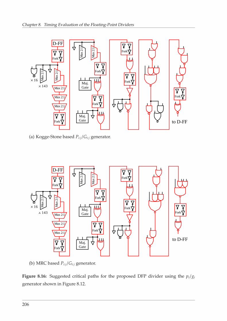
Chapter 8. Timing Evaluation of the Floating-Point Dividers
Fork
D-FF
Fork
Mux
2:1
Mux
2:1
Mux 2:1
Fork
143
16
to D-FF
Mux 2:1
Mux 2:1
Mux
2:1
Mux
2:1
Fork
Fork
Fork
Fork
Maj.Gate
Maj.Gate
(a) Kogge-Stone based Pi: j/Gi: j generator.
Fork
D-FF
Fork
Mux
2:1
Mux
2:1
Mux 2:1
Fork
143
16
to D-FF
Mux 2:1
Mux 2:1
Mux
2:1
Mux
2:1
Fork
ForkFork
Fork
Maj.Gate
Maj.Gate
(b) MRC based Pi: j/Gi: j generator.
Figure 8.16: Suggested critical paths for the proposed DFP divider using the pi/gi
generator shown in Figure 8.12.
206

8.5. DFP Divider Timing Evaluation
Table 8.4: Logical effort calculations on the critical paths in Figures 8.15 and 8.16.
Figure 8.15(a) Figure 8.15(b) Figure 8.16(a) Figure 8.16(b)
Compi LEi pi Compi LEi pi Compi LEi pi Compi LEi pi
D-FF 2 1.7 D-FF 2 1.7 D-FF 2 1.7 D-FF 2 1.72-1 Fork 315.7 2 2-1 Fork 315.7 2 2-1 Fork 315.7 2 2-1 Fork 315.7 2MUX 2:1 2 4 MUX 2:1 2 4 MUX 2:1 2 4 MUX 2:1 2 4MUX 2:1 2 4 MUX 2:1 2 4 MUX 2:1 2 4 MUX 2:1 2 4MUX 2:1 2 4 MUX 2:1 2 4 MUX 2:1 2 4 MUX 2:1 2 4MUX 2:1 2 4 MUX 2:1 2 4 MUX 2:1 2 4 MUX 2:1 2 42-1 Fork 5 2 2-1 Fork 5 2 2-1 Fork 5 2 2-1 Fork 5 2MUX 2:1 2 4 MUX 2:1 2 4 MUX 2:1 2 4 MUX 2:1 2 42-1 Fork 10 2 2-1 Fork 10 2 2-1 Fork 10 2 2-1 Fork 10 2
XOR4 2 8 XOR4 2 8 XOR4 2 8 XOR4 2 82-1 Fork 6 2 2-1 Fork 6 2 2-1 Fork 6 2 2-1 Fork 6 2
XOR4 2 8 XOR4 2 8 XOR4 2 8 XOR4 2 82-1 Fork 6 2 2-1 Fork 6 2 2-1 Fork 6 2 2-1 Fork 6 2
XOR3 2 6 XOR3 2 6 XOR3 2 6 XOR3 2 62-1 Fork 4 2 2-1 Fork 4 2 2-1 Fork 4 2 2-1 Fork 4 2NOR2 3.7 2 NOR2 3.7 2 NOR2 2 2 NOR2 2 2NOR2 2 2 NOR2 3 2 OAI 2.7 2.7 OAI 2.7 2.7AOI 2 3.7 AOI 2 3.7 AOI221 3.3 3.7 AOI221 2 3.7OAI 3.3 2.7 OAI 2 2.7 NAND2 2 2 AOI 2.3 3.7
NAND2 2 2 AOI 2.3 3.7 OAI 2 2.7 OAI221 2 4.3OAI 2 2.7 OAI221 2 4.3 AOI 2 3.7 2-1 Fork 4 2AOI 2 3.7 2-1 Fork 4 2 2-1 Fork 4 2 XNOR2 2 4
2-1 Fork 4 2 XNOR2 2 4 XNOR2 2 4 - - -XNOR2 2 4 - - - - - - - - -
N = 31 N = 30 N = 30 N = 29P = 80.3 P = 80 P = 78.3 P = 78
F = 3641005397333 F = 318587972267 F = 331000490667 F = 115850171733
D = 159.14τ D = 152.54τ D = 150.96τ D = 147.81τ
8.5.3 Logical Effort Calculation
Logical effort calculations of the 4 critical paths’ minimum delays are summarised in
Table 8.4. As shown in the table, the smallest critical path delay
DDFP = 147.81 τ = 29.56 FO4 (8.27)
can be achieved for the proposed DFP divider if the comparison sign detectors are
built using the circuit displayed in Figures 8.12 and 8.14. As a secondary result, due to
similarity between the PR sign detectors and the comparison sign detectors, the former
can be constructed using the same circuit as well.
207

Chapter 8. Timing Evaluation of the Floating-Point Dividers
8.5.4 Division Execution Time
As noted in Subsection 7.6.3, DFP division finishes in p + 3 cycles, where p is the
precision determined from Table 7.2. Considering p = 34 to have the longest execution
time, using the critical path delay (8.27), the division execution time is
DFP divider execution time = 37 × 147.81 τ = 5468.97 τ = 1093.79 FO4 . (8.28)
8.6 Discussion
This section compares the results obtained from the timing evaluations reported in
Sections 8.3, 8.4 and 8.5 with those of the recent designs available in the literature.
8.6.1 Radix-4 FP Divider
Antelo et al [ALMN02] report timing evaluation results for 3 different radix-4 FP di-
viders implemented using high-radix SRT division. They use a pre-layout estimation,
which does not take into account the wiring parasitic capacitance. A 0.35 µm/3.3 V
standard cell library, and Synopsys analysis and synthesis tools are used. The dividers
are as follows.
• Divider, named A for easy referencing, is the original radix-4 FP divider intro-
duced by Ercegovac and Lang [EL94]. This circuit uses a QDS function based on
the traditional selection constant method discussed in Subsection 3.2.3. Since the
PR is represented in the CS format, the QDS function is similar to the structure
shown in Figure 3.8. The quotient is produced after the 29th iteration.
• Divider, named C, is the circuit developed by Burgess and Hinds [BH01]. This
divider, which is explained in Section 4.1.2, employs a technique to pre-load the
corresponding selection constants and performs the selection using the compara-
tors followed by the sign detectors. Divider C requires 29 iterations to calculate
the quotient in the appropriate representation.
• Divider, named D, is the retimed version of Divider C. It is described in Sec-
tion 4.1.3. In Divider D, the QDS function is moved to the end of the recurrence.
This allows the comparison operands to be reordered and therefore, part of the
208

8.6. Discussion
critical path to be transferred to the noncritical part of the divider. A the end of
the 30th iteration, the quotient appears at the output.
Before, starting the discussion on the speed of the designs, it is necessary to sum-
marise the results obtained up until now. To do that, Table 8.5 is constructed containing
the following information.
• The critical path delay and the execution time of Dividers A, C, D calculated by
Antelo et al [ALMN02] using the logic synthesis are reported in both absolute
and FO4 time unit. For that particular technology (0.35 µm/3.3 V), FO4 = 0.15 ns.
• To make a consistent comparison between the designs, the critical path delay
and the execution time of Divider A, which is the fundamental FP divider, are
calculated using the method of logical effort as well as logic synthesis, and re-
ported. The logic synthesis is carried out using Synopsys design compiler (DC)
with Artisan 0.18 µm typical library.
• The recurrence latency and the execution time of Divider E, which is the compar-
ison multiples based radix-4 divider proposed in Chapter 5, are included. These
values reported in Subsections 8.3.4 and 8.3.5 are calculated using the method of
logical effort as well as the logic synthesis. The logic synthesis is carried out using
Synopsys design compiler (DC) with Artisan 0.18 µm typical library.
• In addition to the previously defined dividers, for further clarification on the
sources of the improvements obtained from the new design, a new divider, named
B, is introduced. Divider B is structurally identical to Divider A, however, it has
the comparison multiples based QDS function used in Divider E. In fact, while
Divider A is different from Divider B just in the QDS function, it is distinctive
from Divider E in both the QDS function and the critical path. Therefore, the
effects of the comparison multiples based QDS function and the change in the
divider’s architecture (such as the new critical path) can be studied separately.
For Divider B, the critical path delay and the division execution time are calculated
using the method of logical effort and listed in Table 8.5.
Using the information in Table 8.5, the following comparison cases are possible.
• Logical effort versus logical effort results
For the critical path delays obtained using the method of logical effort, Table 8.5
209

Chapter 8. Timing Evaluation of the Floating-Point Dividers
Table 8.5: Critical path delays and the execution times of Dividers A, B, C, D and E.
Synthesis Logical effort
Iteration delay Execution time Iteration delay Execution time
Design Specification FO4 ns FO4 ns FO4 FO4
21.67a 3.25a 628.43a 94.25a
Divider A– 3.00b – 87.00b
22.53 653.37
Divider B – – – – 18.50 536.50
Divider C 20.67a 3.10a 599.43a 89.90a – –
Divider D 16.00a 2.40a 480.00a 72.00a – –
Divider E – 2.34b – 67.86b 15.63 453.27
a Reported by Antelo et al [ALMN02] for a 0.35 µm/3.3 V process.b Calculated by the author of the thesis for the Artisan 0.18 µm typical library.
shows that Divider B performs FP division about 18% faster than Divider A. Also,
when Divider B is upgraded to Divider E, more than 15% additional speedup is
gained. The table indicates more than 30% decrease in the execution time of
Divider E compared to Divider A.
• Logical effort versus synthesis results
The good correlation between synthesis results and logical effort results for Di-
vider A and Divider E suggests that the two measures are well calibrated and
that comparisons between the two may be tentatively made. Considering delay
of 21.67 FO4 for Divider A and 15.63 FO4 for Divider E, Divider E is almost 28%
faster than the traditional Divider A. This corresponds with the 30% improvement
obtained in the previous comparison case carried out on logical effort results. In
addition, Divider E is about 24% faster than Divider C. Investigating Table 8.5
reveals that moving from Divider D to Divider E achieves more than 2% improve-
ment in the iteration time. However, Divider E responds about 6% faster than
Divider D due to one less iteration required for finishing FP division.
• Synthesis versus synthesis results
Comparing the corresponding latencies listed in Table 8.5 shows 22% speedup
for Divider E comparing to Divider A. This again supports the comparisons
performed in the previous two cases.
210

8.6. Discussion
As an auxiliary result on implementation size, a rough high-level assessment [SHL98,
BN02] states that there is no meaningful difference between the VLSI area of Divider B
and Divider A. However, another evaluation using the same method shows about 25%
increase in the size of Divider E comparing to Divider A. This is due to employing the
adjust circuits and the PR sign detectors, and using more registers and multiplexors.
8.6.2 Radix-16 FP Divider
According to the execution times (8.24) and (8.26), using the radix-16 FP divider in-
troduced in Chapter 5 results in a speedup of 1.2 with respect to the proposed radix-4
building block. This means that the quotient is produced more than 17% faster when
the radix-16 FP divider is used instead of the radix-4 FP divider.
Considering the timing evaluation performed by Nannarelli [Nan99], the execution
time of the radix-16 FP divider developed by Ercegonac and Lang [EL04] is calculated
as 398.74 FO4. This means that the proposed radix-16 comparison multiples based FP
divider is more than 6% faster than the Ercegovac and Lang implementation.
8.6.3 DFP Divider
Realisation of decimal division complying with the requirements of the IEEE 754R
is reported by Wang and Schulte [WS04]. Their design is a Newton-Raphson based
divider, which is different from the proposed DFP divider in nature. However, to the
best of the author’s knowledge, it is the only DFP divider published in the literature.
An estimated critical path delay of 0.69 ns is reported by Wang and Schulte [WS04].
The timing evaluation is obtained from a synthesis using Synopsys Design Compiler
and LSI Logic 0.11 µm gflx-p standard cell library, under nominal operating conditions
and a supply voltage of 1.2 V. In order to make the delays comparable, the reported
critical path delay must be represented in FO4 unit. Using the measure
FO4 ≈ 360 Ldrawn ps , (8.29)
where Ldrawn = 2λ in µm [HMH01], for this specific technology, FO4 is calculated
as FO4 ≈ 40ps conforming to the timing reported by Tamura [Tam04] from Fujitsu
Laboratories. This means that the cycle time of the Newton-Raphson based DFP
divider is about 17 FO4. Wang and Schulte report a latency of 113 cycles for decimal128
operands or equivalently around 1949 FO4. However, this delay can be obtained only
211

Chapter 8. Timing Evaluation of the Floating-Point Dividers
if a sequential decimal multiplier can be found capable of processing 4 decimal digits
per cycle. The proposed DFP divider based on the comparison multiples idea with
execution time of 1094 FO4 is about 1.8 times faster than the ideal Newton-Raphson
based DFP divider. The difference becomes even greater when realistic conditions are
considered for estimating the division execution time. A Newton-Raphson based DFP
divider, which benefits from an initial reciprocal approximation lookup table with a
reasonable size and a sequential fixed-point multiplier with the ability of processing
1 digit per cycle (like that introduced by Earl and Schulte [ES03]), requires 246 cycles
to calculate the quotient. This delay is about 4244 FO4, which is about 4 times the
execution time 1094 FO4 reported in Subsection 8.5.4.
8.7 Summary
In Chapter 8, the critical path delays of the FP dividers developed in Chapters 5 and
7 were estimated using the method of logical effort. Using the delays estimated,
the dividers’ execution times were calculated in both τ and FO4 units. Then, the
calculated execution times were contrasted with the corresponding timing evaluations
reported in the public literature. The comparisons showed that in all the cases the
comparison multiples based FP dividers produced the quotients in shorter times than
their counterparts.
212

Chapter 9
Conclusions and Future Works
Chapter 9 summarises the findings presented in the thesis and discusses some avenues
for future research.
213

Chapter 9. Conclusions and Future Works
9.1 Conclusions
Among all digit recurrence and multiplicative based algorithms, high-radix SRT di-
vision is known to be one of the best approaches for performing FP division [SL96].
This is mainly because of its ability to produce a correctly rounded quotient satis-
fying the IEEE 754 standard [IEE85] in a reasonably short period of time. Many
attempts have been reported to improve the performance of high-radix SRT division
[Tay85, OF95a, OF95b, BW95, HOH97, OF97a, BH01, Kor03]. They try to reduce the
divider critical path delay by minimising the QDS function, finding the best balance
between the radix and the degree of redundancy, developing algorithms resulting in
faster circuits (such as adders/subtractors, multiplexors and comparators) and/or max-
imising the overlap between the design components. While for practical reasons, the
quotient digits are selected from minimally redundant digit sets of radix 4 or at most
8, improving the implementation of the QDS function and increasing the concurrency
are the most effective for reducing the critical path delay. Therefore, the goal of this
thesis is to shorten high-radix SRT division cycle time by developing a more efficient
QDS function, taking some parts of the QDS function off the critical path and breaking
the critical path into two or more parallel but shorter paths. Applying these changes to
high-radix SRT division may result in a FP divider with shorter response time.
9.1.1 Comparison Multiples Approach
In Chapter 4, a new implementation of the QDS function based on the new compar-
ison multiples approach is proposed. In this method, which is mathematically and
architecturally described, instead of searching for the quotient digit in a lookup table,
the quotient digit is directly calculated in the sign and magnitude format. Using the
new representation for the quotient digits, the fan out of some components on the
critical path is almost halved making them operate faster. The QDS function receives
a truncated PR and investigates the range to which the PR belongs. It performs the
examination by comparing the truncated PR with the truncated multiples of the divisor
produced once at the beginning of division. The result of the comparisons are delivered
to a coder in order to produce the magnitude of the quotient digit. Meanwhile another
part of the QDS function, called the PR sign detector, calculates the polarity of the
quotient digit by inspecting the sign of the truncated PR. In the comparison multiples
214

9.1. Conclusions
based QDS function, the PR sign detector operates off the critical path because the quo-
tient digit sign and magnitude are calculated separately. These changes make the QDS
function faster and consequently reduce the divider critical path delay. In addition,
by reordering the components of the recurrence it is possible to merge some circuits
together to further minimise the critical path.
9.1.2 Comparison Multiples Based Radix-4 and Radix-16 FP Divider
To support the argument, Chapter 5 introduces two practical examples of the FP divider
based on the comparison multiples approach. The first is a radix-4 FP divider and
the second is a radix-16 FP divider constructed using two hybrid overlapped radix-4
stages. Applying extended optimisation techniques such as using 2-level multiplexors
and skewing some of the registers make the radix-4 FP divider calculate the quotient
faster and consequently, result in a faster radix-16 FP divider.
9.1.3 Comparison Multiples Based DFP Divider
Due to increasing demand for decimal arithmetic in financial and banking applications,
developing circuits capable of performing arithmetic directly on decimal operands has
become an attractive research topic. While addition, subtraction and multiplication are
much simpler to implement, implementing a divider accepting decimal dividends and
divisors in the recently introduced IEEE 754R standard is a real challenge. Chapter 6
introduces DSD arithmetic, which is a new type of redundant decimal arithmetic.
Based on DSD arithmetic, circuits performing carry-free addition, subtraction and
sign detection on DSD operands are developed. Then, in Chapter 7, using the DSD
components, a DFP divider based on the proposed comparison multiples approach is
introduced. However, since radix 10 is not a power of 2, some minor changes must be
applied to the original approach.
9.1.4 Timing Evaluation
After making sure that the developed radix-4 FP, radix-16 FP and DFP dividers are
functionally correct, timing evaluation is performed on the circuits. In this research,
the method of logical effort is used to estimate the critical path delay of the dividers,
in terms of the technology independent unit of FO4. The calculations carried out in
215

Chapter 9. Conclusions and Future Works
Chapter 8 show that the comparison multiples based radix-4 FP divider is more than
30% faster than a traditional implementation of radix-4 FP division. Moreover, the
logical effort timing estimation reveals that the comparison multiples based radix-16
FP divider produces the quotient more than 17% faster than its radix-4 building block.
Also, the radix-16 divider is over 6% faster than the conventional implementation. The
critical path delay evaluation indicates that the proposed DFP divider is about 4 times
faster than the one available Newton-Raphson based DFP divider.
9.2 Future Work
As discussed in Chapter 3, increasing the radix is one method to achieve a faster
divider. As shown in Chapter 7, the radix of the proposed DFP divider is r = 101,
which results in one decimal quotient digit retired every iteration. As future work
on the DFP dividers, it is very likely to calculate two decimal digits per iteration by
increasing the radix to r = 102 = 100. Another approach toward generating more than
one decimal digit per cycle is to use two stages of the original radix-10 divider and
overlap them appropriately (see Section 3.7). Therefore, although the high-radix DFP
divider will require a larger VLSI area when implemented, a reasonable speedup on
DFP division can be obtained.
Achieving the highest speed in the smallest VLSI area is one of the important goals
when designing a circuit, however, there are some other concerns for the circuit design-
ers to consider. Among them, there is design with low power consumption [RCN02],
which is motivated by battery-operated devices demanding intensive computation in
portable environments. Several techniques have been investigated for reducing the
power consumption in CMOS digital circuits while maintaining computational perfor-
mance. They mainly use the lowest possible supply voltage coupled with architectural,
logic style, circuit and technology optimisation methods [Nan99]. For the proposed
dividers, one may be interested to investigate whether they can be redesigned for low
power without or with only small calculation performance loss.
216

Appendix A
Radix-4 and Radix-16 CRN Units Tables
Table A.1: The truth table of the signals generated by the radix-4 CRN unit. The last
quotient digit q28 is represented as Sign(q28)Mag(q28).
q28 sign Q[27]<52> QM[27]<52> u s1 s0
2 = 111 0 × 0 1 1 1
2 = 111 0 × 1 × 0 0
2 = 111 1 × 0 1 1 1
2 = 111 1 × 1 × 0 0
1 = 110 0 × 0 0 0 0
1 = 110 0 × 1 × 0 0
1 = 110 1 × 0 1 1 1
1 = 110 1 × 1 × 0 0
0 =×00 0 0 × 0 0 0
0 =×00 0 1 × × 0 0
0 =×00 1 0 × 0 0 0
0 =×00 1 1 × × 0 0
1 = 010 0 0 × 1 0 0
1 = 010 0 1 × × 0 0
1 = 010 1 0 × 0 0 0
1 = 010 1 1 × × 0 0
2 = 011 0 0 × 1 0 0
2 = 011 0 1 × × 0 1
2 = 011 1 0 × 1 0 0
2 = 011 1 1 × × 0 0
217

Appendix A. Radix-4 and Radix-16 CRN Units Tables
Table A.2: The truth table of the signals generated by the radix-16 CRN unit. The last
quotient digit is represented as q14 = 4qH14+qL14 = Sign(qH14)Mag(qH14)Sign(qL14)Mag(qL14).
q14 sign Q[13]<50> QM[13]<50> u1 u0 s
10 = 111111 0 × 0 × 001 1
10 = 111111 0 × 1 10 × 1
10 = 111111 1 × 0 × 001 1
10 = 111111 1 × 1 01 × 1
9 = 111110 0 × 0 × 100 1
9 = 111110 0 × 1 10 × 1
9 = 111110 1 × 0 × 011 1
9 = 111110 1 × 1 10 × 1
8 = 111×00 0 × 0 × 100 1
8 = 111×00 0 × 1 10 × 1
8 = 111×00 1 × 0 × 100 1
8 = 111×00 1 × 1 10 × 1
7 = 111010 0 × 0 × 101 1
7 = 111010 0 × 1 10 × 1
7 = 111010 1 × 0 × 100 1
7 = 111010 1 × 1 10 × 1
6 = 111011 0 × 0 × 101 1
6 = 111011 0 × 1 11 × 1
6 = 111011 1 × 0 × 101 1
6 = 111011 1 × 1 10 × 1
6 = 110111 0 × 0 × 101 1
6 = 110111 0 × 1 11 × 1
6 = 110111 1 × 0 × 101 1
6 = 110111 1 × 1 10 × 1
5 = 110110 0 × 0 × 110 1
5 = 110110 0 × 1 11 × 1
5 = 110110 1 × 0 × 101 1
5 = 110110 1 × 1 11 × 1
4 = 110×00 0 × 0 × 110 1
4 = 110×00 0 × 1 11 × 1
4 = 110×00 1 × 0 × 110 1
4 = 110×00 1 × 1 11 × 1
Continued on next page
218

A.0. Future Work
Table A.2: – continues from previous page
q14 sign Q[13]<50> QM[13]<50> u1 u0 s
3 = 110010 0 × 0 × 111 1
3 = 110010 0 × 1 11 × 1
3 = 110010 1 × 0 × 110 1
3 = 110010 1 × 1 11 × 1
2 = 110011 0 × 0 × 111 1
2 = 110011 0 × 1 00 × 0
2 = 110011 1 × 0 × 111 1
2 = 110011 1 × 1 11 × 1
2 =×00111 0 × 0 × 111 1
2 =×00111 0 × 1 00 × 0
2 =×00111 1 × 0 × 111 1
2 =×00111 1 × 1 11 × 1
1 =×00110 0 × 0 × 000 0
1 =×00110 0 × 1 00 × 0
1 =×00110 1 × 0 × 111 1
1 =×00110 1 × 1 00 × 0
0 =×00×00 0 0 × × 000 0
0 =×00×00 0 1 × 00 × 0
0 =×00×00 1 0 × × 000 0
0 =×00×00 1 1 × 00 × 0
1 =×00010 0 0 × × 001 0
1 =×00010 0 1 × 00 × 0
1 =×00010 1 0 × × 000 0
1 =×00010 1 1 × 00 × 0
2 =×00011 0 0 × × 001 0
2 =×00011 0 1 × 01 × 0
2 =×00011 1 0 × × 001 0
2 =×00011 1 1 × 00 × 0
2 = 010111 0 0 × × 001 0
2 = 010111 0 1 × 01 × 0
2 = 010111 1 0 × × 001 0
2 = 010111 1 1 × 00 × 0
3 = 010110 0 0 × × 010 0
3 = 010110 0 1 × 01 × 0
3 = 010110 1 0 × × 001 0
Continued on next page
219

Appendix A. Radix-4 and Radix-16 CRN Units Tables
Table A.2: – continues from previous page
q14 sign Q[13]<50> QM[13]<50> u1 u0 s
3 = 010110 1 1 × 01 × 0
4 = 010×00 0 0 × × 010 0
4 = 010×00 0 1 × 01 × 0
4 = 010×00 1 0 × × 010 0
4 = 010×00 1 1 × 01 × 0
5 = 010010 0 0 × × 011 0
5 = 010010 0 1 × 01 × 0
5 = 010010 1 0 × × 010 0
5 = 010010 1 1 × 01 × 0
6 = 010011 0 0 × × 011 0
6 = 010011 0 1 × 10 × 0
6 = 010011 1 0 × × 011 0
6 = 010011 1 1 × 01 × 0
6 = 011111 0 0 × × 011 0
6 = 011111 0 1 × 10 × 0
6 = 011111 1 0 × × 011 0
6 = 011111 1 1 × 01 × 0
7 = 011110 0 0 × × 100 0
7 = 011110 0 1 × 10 × 0
7 = 011110 1 0 × × 011 0
7 = 011110 1 1 × 10 × 0
8 = 011×00 0 0 × × 100 0
8 = 011×00 0 1 × 10 × 0
8 = 011×00 1 0 × × 100 0
8 = 011×00 1 1 × 10 × 0
9 = 011010 0 0 × × 101 0
9 = 011010 0 1 × 10 × 0
9 = 011010 1 0 × × 100 0
9 = 011010 1 1 × 10 × 0
10 = 011011 0 0 × × 101 0
10 = 011011 0 1 × 11 × 0
10 = 011011 1 0 × × 101 0
10 = 011011 1 1 × 10 × 0
220

Appendix B
VHDL Code of the Radix-4 Divider
B.1 adjust.vhd
library ieee;
use ieee.std_logic_1164.all;
use ieee.std_logic_arith.all;
use ieee.std_logic_unsigned.all;
entity adjust is
port(
s0p, s0m, s1p, s1m, s2p, s2m : in
std_logic_vector(2 downto 0); w0p, w0m, w1p, w1m, w2p, w2m : out
std_logic_vector(1 downto 0));
end adjust;
architecture behavioral of adjust is
begin process(s0p, s0m, s1p, s1m, s2p, s2m)
begin
if s0p(2) = s0m(2) then
w0p <= s0p(1 downto 0);
w0m <= s0m(1 downto 0);
elsif s0p(1) = s0m(1) then
w0p <= s0m(0) & s0m(0);
w0m <= s0p(0) & s0p(0);
else
w0p <= s0m(1) & s0p(0);
w0m <= s0p(1) & s0m(0);
end if;
221

Appendix B. VHDL Code of the Radix-4 Divider
if s1p(2) = s1m(2) then
w1p <= s1p(1 downto 0);
w1m <= s1m(1 downto 0);
elsif s1p(1) = s1m(1) then
w1p <= s1m(0) & s1m(0);
w1m <= s1p(0) & s1p(0);
else
w1p <= s1m(1) & s1p(0);
w1m <= s1p(1) & s1m(0);
end if;
if s2p(2) = s2m(2) then
w2p <= s2p(1 downto 0);
w2m <= s2m(1 downto 0);
elsif s2p(1) = s2m(1) then
w2p <= s2m(0) & s2m(0);
w2m <= s2p(0) & s2p(0);
else
w2p <= s2m(1) & s2p(0);
w2m <= s2p(1) & s2m(0);
end if;
end process;
end behavioral;
B.2 compsd.vhd
library ieee;
use ieee.std_logic_1164.all;
use ieee.std_logic_arith.all;
use ieee.std_logic_unsigned.all;
entity compsd is
port(
p1p, p1m, p2p, p2m : in std_logic_vector(6 downto 0);
sign : in std_logic;
q1 , q0 : out std_logic);
end compsd;
architecture behavioral of compsd is
signal sm1, sm2 : std_logic;
begin
222

B.3. comparator.vhd
process(p1p, p1m, p2p, p2m)
begin
if (p1p >= p1m) then
sm1 <= ’0’;
else
sm1 <= ’1’;
end if;
if (p2p >= p2m) then
sm2 <= ’0’;
else
sm2 <= ’1’;
end if;
end process;
q1 <= sm1 xnor sign;
q0 <= sm2 xnor sign;
end behavioral;
B.3 comparator.vhd
library ieee;
use ieee.std_logic_1164.all;
use ieee.std_logic_arith.all;
use ieee.std_logic_unsigned.all;
entity comparator is
port(
rwp, rwm, m1_xnor, m2_xnor : in std_logic_vector(6 downto 0);
sign : in std_logic;
p1p, p1m, p2p, p2m : out std_logic_vector(6 downto 0));
end comparator;
architecture behavioral of comparator is
begin
process(rwp, rwm, sign, m1_xnor, m2_xnor)
begin
for i in 0 to 5 loop
p1p(i+1) <= not (rwp(i) xor (not rwm(i)) xor m1_xnor(i));
p1m(i) <= (rwp(i) and (not rwm(i))) or (m1_xnor(i)
and rwp(i)) or (m1_xnor(i) and (not rwm(i)));
end loop;
223

Appendix B. VHDL Code of the Radix-4 Divider
p1m(6) <= (rwp(6) and (not rwm(6))) or (m1_xnor(6) and
rwp(6)) or (m1_xnor(6) and (not rwm(6)));
p1p(0) <= not sign;
for i in 0 to 5 loop
p2p(i+1) <= not (rwp(i) xor (not rwm(i)) xor m2_xnor(i));
p2m(i) <= (rwp(i) and (not rwm(i))) or (m2_xnor(i)
and rwp(i)) or (m2_xnor(i) and (not rwm(i)));
end loop;
p2m(6) <= (rwp(6) and (not rwm(6))) or (m2_xnor(6) and
rwp(6)) or (m2_xnor(6) and (not rwm(6)));
p2p(0) <= not sign;
end process;
end behavioral;
B.4 critical.vhd
library ieee;
use ieee.std_logic_1164.all;
use ieee.std_logic_arith.all;
use ieee.std_logic_unsigned.all;
entity critical is
port(
m1, m2, w2p, w1p, x, w0p,
w2m, w1m, w0m : in std_logic_vector(6 downto 0);
clk, sign2, sign1, sign0 : in std_logic;
q1q0_non : out std_logic_vector(1 downto 0));
end critical;
architecture behavioral of critical is
component ff
generic(
n : integer );
port(
clk : in std_logic;
din : in std_logic_vector(n - 1 downto 0);
dout : out std_logic_vector(n - 1 downto 0));
end component;
component mux1muxs
generic(
224

B.4. critical.vhd
n : integer);
port(
signx_out, sign0_out, sign1_out, sign2_out : in std_logic;
q1q0 : in std_logic_vector(1 downto 0);
w0p_out, w2m_out, w1m_out, w0m_out : in std_logic_vector(n - 1 downto 0);
w2p_out, w1p_out, x : in std_logic_vector(n - 1 downto 0);
rwp, rwm : out std_logic_vector(n - 1 downto 0);
sign : out std_logic);
end component;
component qds
port(
sign : in std_logic;
rwp, rwm, m1, m2 : in std_logic_vector(6 downto 0);
q1, q0 : out std_logic);
end component;
signal rwp, rwm : std_logic_vector(6 downto 0);
signal q1q0_out : std_logic_vector(1 downto 0);
signal sign, q1_out, q0_out, q1, q0 : std_logic;
signal q1_tmp, q0_tmp, q1_out_tmp, q0_out_tmp : std_logic_vector(0 downto 0);
begin
q1_ff: ff
generic map(
n => 1)
port map(
clk => clk,
din => q1_tmp,
dout => q1_out_tmp);
q1_tmp(0) <= q1;
q1_out <= q1_out_tmp(0);
q0_ff: ff
generic map(
n => 1)
port map(
clk => clk,
din => q0_tmp,
dout => q0_out_tmp);
q0_tmp(0) <= q0;
q0_out <= q0_out_tmp(0);
q1q0_out <= q1_out & q0_out;
q1q0_non <= q1q0_out;
225

Appendix B. VHDL Code of the Radix-4 Divider
mux: mux1muxs
generic map(
n => 7)
port map(
signx_out => sign0,
sign0_out => sign0,
sign1_out => sign1,
sign2_out => sign2,
q1q0 => q1q0_out,
w2p_out => w2p,
w1p_out => w1p,
x => x,
w0p_out => w0p,
w2m_out => w2m,
w1m_out => w1m,
w0m_out => w0m,
rwp => rwp,
rwm => rwm,
sign => sign);
qds_r4: qds
port map(
sign => sign,
rwp => rwp,
rwm => rwm,
m1 => m1,
m2 => m2,
q1 => q1,
q0 => q0);
end behavioral;
B.5 divider.vhd
library ieee;
use ieee.std_logic_1164.all;
use ieee.std_logic_arith.all;
use ieee.std_logic_unsigned.all;
entity divider is
port(
x, d : in std_logic_vector(54 downto 0);
226

B.5. divider.vhd
clk : in std_logic;
sq1q0 : out std_logic_vector(2 downto 0));
end divider;
architecture behavioral of divider is
component critical
port(
m1, m2, w2p, w1p, x, w0p, w2m, w1m, w0m : in std_logic_vector(6 downto 0);
clk, sign2, sign1, sign0 : in std_logic;
q1q0_non : out std_logic_vector(1 downto 0)
sign_non : out std_logic);
end component;
component ff
generic(
n : integer);
port(
clk : in std_logic;
din : in std_logic_vector(n - 1 downto 0);
dout : out std_logic_vector(n - 1 downto 0));
end component;
component mux1muxs
generic(
n : integer);
port(
signx_out, sign0_out, sign1_out, sign2_out : in std_logic;
q1q0 : in std_logic_vector(1 downto 0);
w0p_out, w2m_out, w1m_out, w0m_out : in std_logic_vector(n - 1 downto 0);
w2p_out, w1p_out, x : in std_logic_vector(n - 1 downto 0);
rwp, rwm : out std_logic_vector(n - 1 downto 0);
sign : out std_logic);
end component;
component prformation
port (
rwp, rwm, d1_xnor, d2_xnor : in std_logic_vector(56 downto 0);
sign : in std_logic;
s0p, s0m, s1p, s1m, s2p, s2m : out std_logic_vector(57 downto 0));
end component;
component prsd
port (
s0p, s0m, s1p, s1m, s2p, s2m : in std_logic_vector(6 downto 0);
227

Appendix B. VHDL Code of the Radix-4 Divider
sign0, sign1, sign2 : out std_logic);
end component;
component adjust
port (
s0p, s0m, s1p, s1m, s2p, s2m : in std_logic_vector(2 downto 0);
w0p, w0m, w1p, w1m, w2p, w2m : out std_logic_vector(1 downto 0));
end component;
component multiplegen
port(
d : in std_logic_vector(54 downto 0);
sign : in std_logic;
d1_xnor, d2_xnor : out std_logic_vector(56 downto 0));
end component;
signal s0p, s0m, s1p, s1m, s2p, s2m : std_logic_vector(57 downto 0);
signal d1_xnor, d2_xnor, rwp, rwm : std_logic_vector(56 downto 0);
signal w0m_out, w1p_out, w1m_out, w2p_out, w2m_out : std_logic_vector(54 downto 0);
signal w0p, w0m, w1p, w1m, w2p, w2m : std_logic_vector(54 downto 0);
signal m1, m2 : std_logic_vector(6 downto 0);
signal q1q0 : std_logic_vector(1 downto 0);
signal sign, sign0, sign1, sign2, sign0_out, sign1_out, sign2_out : std_logic;
signal sign1_out_tmp, sign2_tmp, sign2_out_tmp : std_logic_vector(0 downto 0);
signal sign0_tmp, sign0_out_tmp, sign1_tmp : std_logic_vector(0 downto 0);
begin
m1 <= "000" & d(54 downto 51);
m2 <= ’0’ & (d(54 downto 49) - ("00" & d(54 downto 51)));
sq1q0 <= sign & q1q0;
d1 <= ’0’ & d & ’0’;
d2 <= d & "00";
w0pff: ff
generic map(
n => 55)
port map(
clk => clk,
din => w0p,
dout => w0p_out);
w0mff: ff
generic map(
n => 55)
port map(
clk => clk,
228

B.5. divider.vhd
din => w0m,
dout => w0m_out);
w1pff: ff
generic map(
n => 55)
port map(
clk => clk,
din => w1p,
dout => w1p_out);
w1mff: ff
generic map(
n => 55)
port map(
clk => clk,
din => w1m,
dout => w1m_out);
w2pff: ff
generic map(
n => 55)
port map(
clk => clk,
din => w2p,
dout => w2p_out);
w2mff: ff
generic map(
n => 55)
port map(
clk => clk,
din => w2m,
dout => w2m_out);
s0: ff
generic map(
n => 1)
port map(
clk => clk,
din => sign0_tmp,
dout => sign0_out_tmp);
sign0_tmp(0) <= sign0;
sign0_out <= sign0_out_tmp(0);
s1: ff
229

Appendix B. VHDL Code of the Radix-4 Divider
generic map(
n => 1)
port map(
clk => clk,
din => sign1_tmp,
dout => sign1_out_tmp);
sign1_tmp(0) <= sign1;
sign1_out <= sign1_out_tmp(0);
s2: ff
generic map(
n => 1)
port map(
clk => clk,
din => sign2_tmp,
dout => sign2_out_tmp);
sign2_tmp(0) <= sign2;
sign2_out <= sign2_out_tmp(0);
mux1muxs: mux1muxs
generic map(
n => 48)
port map(
q1q0 => q1q0,
signx_out => sign0_out,
sign0_out => sign0_out,
sign1_out => sign1_out,
sign2_out => sign2_out,
w2p_out => w2p_out(47 downto 0),
w1p_out => w1p_out(47 downto 0),
x => x(47 downto 0),
w0p_out => w0p_out(47 downto 0),
w2m_out => w2m_out(47 downto 0),
w1m_out => w1m_out(47 downto 0),
w0m_out => w0m_out(47 downto 0),
rwp => rwp(49 downto 2),
rwm => rwm(49 downto 2),
sign => sign);
critical_path: critical
port map(
m1 => m1,
m2 => m2,
230

B.5. divider.vhd
w2p => w2p_out(54 downto 48),
w1p => w1p_out(54 downto 48),
x => x(54 downto 48),
w0p => w0p_out(54 downto 48),
w2m => w2m_out(54 downto 48),
w1m => w1m_out(54 downto 48),
w0m => w0m_out(54 downto 48),
clk => clk,
sign2 => sign2_out,
sign1 => sign1_out,
sign0 => sign0_out,
q1q0_non => q1q0);
mult_gen: multiplegen
port map(
d => d,
sign => sign,
d1_xnor => d1_xnor,
d2_xnor => d2_xnor);
pr_form: prformation
port map (
rwp => rwp,
rwm => rwm,
d1_xnor => d1_xnor,
d2_xnor => d2_xnor,
sign => sign,
s0p => s0p,
s0m => s0m,
s1p => s1p,
s1m => s1m,
s2p => s2p,
s2m => s2m);
pr_sign_det: prsd
port map(
s0p => s0p(57 downto 51),
s0m => s0m(57 downto 51),
s1p => s1p(57 downto 51),
s1m => s1m(57 downto 51),
s2p => s2p(57 downto 51),
s2m => s2m(57 downto 51),
sign0 => sign0,
231

Appendix B. VHDL Code of the Radix-4 Divider
sign1 => sign1,
sign2 => sign2);
adj: adjust
port map(
s0p => s0p(55 downto 53),
s0m => s0m(55 downto 53),
s1p => s1p(55 downto 53),
s1m => s1m(55 downto 53),
s2p => s2p(55 downto 53),
s2m => s2m(55 downto 53),
w0p => w0p(54 downto 53),
w0m => w0m(54 downto 53),
w1p => w1p(54 downto 53),
w1m => w1m(54 downto 53),
w2p => w2p(54 downto 53),
w2m => w2m(54 downto 53));
w0p(52 downto 0) <= s0p(52 downto 0);
w0m(52 downto 0) <= s0m(52 downto 0);
w1p(52 downto 0) <= s1p(52 downto 0);
w1m(52 downto 0) <= s1m(52 downto 0);
w2p(52 downto 0) <= s2p(52 downto 0);
w2m(52 downto 0) <= s2m(52 downto 0);
end behavioral;
B.6 ff.vhd
library ieee;
use ieee.std_logic_1164.all;
use ieee.std_logic_arith.all;
use ieee.std_logic_unsigned.all;
entity ff is
generic(
n : integer := 8);
port(
clk : in std_logic;
din : in std_logic_vector(n - 1 downto 0);
dout : out std_logic_vector(n - 1 downto 0));
end ff;
232

B.8. multiplegen.vhd
architecture behavioral of ff is
begin
process (clk)
begin
if clk’event and clk=’1’ then --clk rising edge
dout <= din;
end if;
end process;
end behavioral;
B.7 m1m2invert.vhd
library ieee;
use ieee.std_logic_1164.all;
use ieee.std_logic_arith.all;
use ieee.std_logic_unsigned.all;
entity m1m2invert is
port(
sign : in std_logic;
m1, m2 : in std_logic_vector(6 downto 0);
m1_xnor, m2_xnor : out std_logic_vector(6 downto 0));
end m1m2invert;
architecture behavioral of m1m2invert is
begin
process(sign, m1, m2)
begin
for i in m1’range loop
m1_xnor(i) <= m1(i) xnor sign;
m2_xnor(i) <= m2(i) xnor sign;
end loop;
end process;
end behavioral;
B.8 multiplegen.vhd
library ieee;
use ieee.std_logic_1164.all;
use ieee.std_logic_arith.all;
233

Appendix B. VHDL Code of the Radix-4 Divider
use ieee.std_logic_unsigned.all;
entity multiplegen is
port(
d : in std_logic_vector(54 downto 0);
sign : in std_logic;
d1_xnor, d2_xnor : out std_logic_vector(56 downto 0));
end multiplegen;
architecture behavioral of multiplegen is
signal d_tmp : std_logic_vector(54 downto 0);
begin
mult_gen: process(d, sign)
begin
for i in d’range loop
d_tmp(i) <= d(i) xnor sign;
end loop;
end process;
d1_xnor <= (not sign) & (not sign) & d_tmp;
d2_xnor <= (not sign) & d_tmp & (not sign);
end behavioral;
B.9 mux1muxs.vhd
library ieee;
use ieee.std_logic_1164.all;
use ieee.std_logic_arith.all;
use ieee.std_logic_unsigned.all;
entity mux1muxs is
generic(
n : integer := 7);
port(
signx_out, sign0_out, sign1_out, sign2_out : in std_logic;
q1q0 : in std_logic_vector(1 downto 0);
w0p_out, w2m_out, w1m_out, w0m_out : in std_logic_vector(n - 1 downto 0);
w2p_out, w1p_out, x : in std_logic_vector(n - 1 downto 0);
rwp, rwm : out std_logic_vector(n - 1 downto 0);
sign : out std_logic);
end mux1muxs;
234

B.10. prformation.vhd
architecture behavioral of mux1muxs is
signal zero : std_logic_vector(n - 1 downto 0);
begin
mux1: process (q1q0, w2p_out, w1p_out, x, w0p_out, w2m_out, w1m_out, w0m_out)
begin
for i in 0 to n - 1 loop
zero(i) <= ’0’;
end loop;
case q1q0 is
when "00" =>
rwp <= w0p_out;
rwm <= w0m_out;
when "01" =>
rwp <= x;
rwm <= zero;
when "10" =>
rwp <= w1p_out;
rwm <= w1m_out;
when "11" =>
rwp <= w2p_out;
rwm <= w2m_out;
when others => null;
end case;
end process;
muxs: process(q1q0, signx_out, sign0_out, sign1_out, sign2_out)
begin
case q1q0 is
when "00" =>
sign <= sign0_out;
when "01" =>
sign <= signx_out;
when "10" =>
sign <= sign1_out;
when "11" =>
sign <= sign2_out;
when others => null;
end case;
end process;
end behavioral;
235

Appendix B. VHDL Code of the Radix-4 Divider
B.10 prformation.vhd
library ieee;
use ieee.std_logic_1164.all;
use ieee.std_logic_arith.all;
use ieee.std_logic_unsigned.all;
entity prformation is
port (
rwp, rwm, d1_xnor, d2_xnor : in std_logic_vector(56 downto 0);
sign : in std_logic;
s0p, s0m, s1p, s1m, s2p, s2m : out std_logic_vector(57 downto 0));
end prformation;
architecture behavioral of prformation is
begin
process(rwp, rwm, sign, d1_xnor, d2_xnor)
begin
s1p(0) <= not sign;
s1m(57) <= not sign;
s2p(0) <= not sign;
s2m(57) <= not sign;
s0p <= ’0’ & rwp;
s0m <= ’0’ & rwm;
for i in 0 to 56 loop
s1p(i+1) <= not (rwp(i) xor (not rwm(i)) xor d1_xnor(i));
s1m(i) <= (rwp(i) and (not rwm(i))) or (d1_xnor(i)
and rwp(i)) or (d1_xnor(i) and (not rwm(i)));
s2p(i+1) <= not (rwp(i) xor (not rwm(i)) xor d2_xnor(i));
s2m(i) <= (rwp(i) and (not rwm(i))) or (d2_xnor(i)
and rwp(i)) or (d2_xnor(i) and (not rwm(i)));
end loop;
end process;
end behavioral;
B.11 prsd.vhd
library ieee;
use ieee.std_logic_1164.all;
use ieee.std_logic_arith.all;
236

B.12. qds.vhd
use ieee.std_logic_unsigned.all;
entity prsd is
port(
s0p, s0m, s1p, s1m, s2p, s2m : in std_logic_vector(6 downto 0);
sign0, sign1, sign2 : out std_logic);
end prsd;
architecture behavioral of prsd is
begin
process(s2p, s2m, s1p, s1m, s0p, s0m)
begin
if s2p >= s2m then
sign2 <= ’0’;
else
sign2 <= ’1’;
end if;
if s1p >= s1m then
sign1 <= ’0’;
else
sign1 <= ’1’;
end if;
if s0p >= s0m then
sign0 <= ’0’;
else
sign0 <= ’1’;
end if;
end process;
end behavioral;
B.12 qds.vhd
library ieee;
use ieee.std_logic_1164.all;
use ieee.std_logic_arith.all;
use ieee.std_logic_unsigned.all;
entity qds is
port(
sign : in std_logic;
237

Appendix B. VHDL Code of the Radix-4 Divider
rwp, rwm, m1, m2 : in std_logic_vector(6 downto 0);
q1, q0 : out std_logic);
end qds;
architecture behavioral of qds is
component comp_sd
port(
p1p, p1m, p2p, p2m : in std_logic_vector(6 downto 0);
sign : in std_logic;
q1 , q0 : out std_logic);
end component;
component m1m2invert
port(
sign : in std_logic;
m1, m2 : in std_logic_vector(6 downto 0);
m1_xnor, m2_xnor : out std_logic_vector(6 downto 0));
end component;
component comparator
port(
rwp, rwm, m1_xnor, m2_xnor : in std_logic_vector(6 downto 0);
sign : in std_logic;
p1p, p1m, p2p, p2m : out std_logic_vector(6 downto 0));
end component;
signal m1_xnor, m2_xnor, p1p, p1m, p2p, p2m : std_logic_vector(6 downto 0);
begin
m1m2_inv: m1m2invert
port map(
sign => sign,
m1 => m1,
m2 => m2,
m1_xnor => m1_xnor,
m2_xnor => m2_xnor);
comparators: comparator
port map(
rwp => rwp,
rwm => rwm,
m1_xnor => m1_xnor,
m2_xnor => m2_xnor,
sign => sign,
238

B.12. qds.vhd
p1p => p1p,
p1m => p1m,
p2p => p2p,
p2m => p2m);
comp_sign_det: compsd
port map(
p1p => p1p,
p1m => p1m,
p2p => p2p,
p2m => p2m,
sign => sign,
q1 => q1,
q0 => q0);
end behavioral;
239

Appendix B. VHDL Code of the Radix-4 Divider
240

BIBLIOGRAPHY
Bibliography
[AK74] D. E. Atkins and V. U. Kalaycioglu. Concurrency in Generalized Radix,
Non-restoring Division. In Proceedings 12th Allerton Conference on Circuit
and Switching Theory, pages 628–640, Illinois, USA, October 1974. Univer-
sity of Illinois.
[ALB98] E. Antelo, T. Lang, and J. D. Bruguera. Computation of√
x/d in a Very
High Radix Combined Division/Square-Root Unit with Scaling and Se-
lection by Rounding. IEEE Transactions on Computers, 47(2):152–161, Feb-
ruary 1998.
[ALMN02] E. Antelo, T. Lang, P. Montuschi, and A. Nannarelli. Fast Radix-4 Re-
timed Division with Selection by Comparisons. In Proceedings of the IEEE
International Conference on Application-Specific Systems, Architectures, and
Processors (ASAP’02), pages 185–196, San Jose, CA, USA, 17–19 July 2002.
[Amr99] B. Amrutur. Design and Analysis of Fast Low Power SRAMs. PhD thesis,
Stanford Univerisy, Stanford, CA, USA, August 1999.
[Atk67] D. E. Atkins. The Theory and Implementation of SRT Division. Technical
Report UIUCDCS-R-67-230, Department of Computer Science, University
of Illinois at Urbana-Champaign, Urbana, Illinois, USA, 1967.
[Atk68] D. E. Atkins. Higher-Radix Division Using Estimates of the Divisor and
Partial Remainders. IEEE Transactions on Computers, C-17:925–934, 1968.
[Atk70] D. E. Atkins. A Study of Methods for Selection of Quotient Digits during
Digital Division. PhD thesis, Department of Computer Science, University
of Illinois at Urbana-Champaign, Urbana, Illinois, USA, 1970.
241

BIBLIOGRAPHY
[Avi61] A. Avizienis. Signed-Digit Number Representations for Fast Parallel
Arithmetic. IRE Transactions on Electronic Computers, EC-10:389–400, Sep-
tember 1961.
[BH01] N. Burgess and C. Hinds. Design Issues in Radix-4 SRT Square Root
and Divide Unit. In Proceedings of the 35th Asilomar Conference on Signals,
Systems and Computers (ASILOMAR’01), pages 1646–1650, Pacific Grove,
CA, USA, 4–7 November 2001.
[BK82] R. P. Brent and H. T. Kung. A Regular Layout for Parallel Adders. IEEE
Transactions on Electronic Computers, C-31(3):260–264, March 1982.
[BKL+01] F. Y. Busaba, C. A. Krygowski, W. H. Li, E. M. Schwarz, and S. R. Carlough.
The IBM z900 Decimal Arithmetic Unit. In Proceedings of the 35th Asilomar
Conference on Signals, Systems and Computers (ASILOMAR’01), pages 1335–
1339, Pacific Grove, CA, USA, 4–7 November 2001.
[BL00] J. D. Bruguera and T. Lang. Multilevel Reverse-Carry Adder. In Proceed-
ings of the 2000 IEEE International Conference on Computer Design: VLSI
in Computers & Processors (ICCD2000), pages 155–162, Austin, TX, USA,
17–20 September 2000. IEEE Computer Society.
[BL01] J. D. Bruguera and T. Lang. Using the Reverse-Carry Approach for Dou-
ble Datapath Floating-Point Addition. In Proceedings of the 15th IEEE
Symposium on Computer Arithmetic (ARITH-15’01), pages 203–210, Vail,
Colorado, USA, 11–13 June 2001. IEEE Computer Society Press.
[BL03] J. D. Bruguera and T. Lang. Multilevel Reverse-Carry Addition: Single
and Dual Adders. The Journal of VLSI Signal Processing-Systems for Signal,
Image, and Video Technology, 33(1–2):55–74, January–February 2003.
[Bla98] G. M. Blair. The Equivalence of Twos-Complement Addition and the
Conversion of Redundant-Binary to Twos-Complement Numbers. Trans-
actions on Circuits and Systems I, 45(6):669–671, July 1998.
[BN02] K. M. Buyukshahin and F. N. Najm. High-Level Area Estimation. In
ISLPED ’02: Proceedings of the 2002 international symposium on Low power
242

BIBLIOGRAPHY
electronics and design, pages 271–274, New York, NY, USA, 2002. ACM
Press.
[BPPT87] B. K. Bose, D. A. Patterson, L. Pei, and G. S. Taylor. Fast Multiply and
Divide for a VLSI Floating-Point Unit. In Proceedings of the 8th IEEE
Symposium on Computer Arithmetic (ARITH-8’87), Como, Italy, 19–21 May
1987. IEEE Computer Society Press.
[Bry96] R. E. Bryant. Bit-Level Analysis of an SRT Divider Circuit. In Proceedings
of the 33rd Annual Conference on Design Automation, pages 661–665, Las
Vegas, NV, USA, June 1996. ACM Press.
[Bur91] N. Burgess. Radix-2 SRT Division Algorithm with Simple Quotient Digit
Selection. Electronics Letters, 27(21):1910–1911, October 1991.
[Bur03a] N. Burgess. Logical Effort Analysis of a Media-Enhanced Adder. In
Proceedings of the 37th Asilomar Conference on Signals, Systems and Computers
(ASILOMAR’03), pages 344–348, Pacific Grove, CA, USA, 9–12 November
2003.
[Bur03b] N. Burgess. Logical Effort Analysis of Register File Architectures. In
Proceedings of the 37th Asilomar Conference on Signals, Systems and Computers
(ASILOMAR’03), Pacific Grove, CA, USA, 9–12 November 2003.
[BW95] N. Burgess and T. Williams. Choices of Operand Truncation in the SRT
Division Algorithm. IEEE Transactions on Computers, 44(7):933–938, 1995.
[CBF01] A. Chandrakasan, W. J. Bowhill, and F. Fox, editors. Design of High-
Performance Microprocessor Circuits. John Wiley & Sons and IEEE Press,
2001.
[CC99] G. Cornetta and J. Cortadella. A Radix-16 SRT Division Unit with Spec-
ulation of the Quotient Digits. In Proceedings of the Ninth Great Lakes
Symposium on VLSI (GLS-VLSI‘99), pages 74–77, Ann Arbor, MI, USA, 4–6
March 1999. IEEE Computer Society Press.
[CCA03] P. Celinski, S. D. Cotofana, and D. Abbott. Logical Effort Delay Modeling
of Sense Amplifier Based Charge Recycling Threshold Logic Gates. In
243

BIBLIOGRAPHY
Proceedings of the 14th Annual Workshop on Circuits, Systems and Signal
Processing (ProRISC 2003), pages 43–48, November 2003.
[CCT00] J. S. Chiang, H. D. Chung, and M. S. Tsai. Carry-Free Radix-2 Subtractive
Division Algorithm and Implementation of the Divider. Tamkang Journal
of Science and Engineering, 3(4):249–255, 2000.
[CH75] T. C. Chen and I. T. Ho. Storage-Efficient Representation of Decimal Data.
Communications of the ACM, 18(1):49–52, 1975.
[Cli90] W. D. Clinger. How to Read Floating Point Numbers Accurately. In
Proceedings of the Conference on Programming Language Design and Imple-
mentation, pages 92–101, White Plains, NY, USA, June 1990. ACM Press.
[CM91] L. Ciminiera and P. Montuschi. Simple Radix 2 Division and Square Root
with Skipping Some Addition Steps. In Proceedings of the 10th IEEE Sym-
posium on Computer Arithmetic (ARITH-10’91), pages 202–209, Grenoble,
France, 26–28 June 1991. IEEE Computer Society Press.
[CNI95] R. M. Owens C. Nagendra and M. J. Irwin. Unifying Carry-Sum and
Signed-Digit Number Representations for Low Power. In Proceedings of
International Symposium on Low Power Design ISLPD’95, pages 15–20, Dana
Point, CA, USA, April 23–26 1995. ACM-SIGDA and IEEE-CAS.
[Com04] IEEE Standard Committee. Some Proposals for Revising ANSI/IEEE Std
754-1985. http://754r.ucbtest.org/, 21 July 2004.
[Cow02] M. Cowlishaw. Densely Packed Decimal Encoding. IEE Proceedings -
Computers and Digital Techniques, 142(3):102–104, May 2002.
[Cow03a] M. Cowlishaw. Decimal Arithmetic Encoding Strawman 4d.
http://www2.hursley.ibm.com/decimal/decbits.pdf, 21 February 2003.
[Cow03b] M. F. Cowlishaw. Decimal Floating-Point: Algorism for Computers. In
Proceedings of the 16th IEEE Symposium on Computer Arithmetic (ARITH-
16’03), pages 104–111, Santiago de Compostela, Spain, 15–18 June 2003.
IEEE Computer Society Press.
244

BIBLIOGRAPHY
[Cow04] M. Cowlishaw. General Decimal Arithmetic Specification – Version 1.45.
http://www2.hursley.ibm.com/decimal/decarith.pdf, 2 August 2004.
[CS57] J. Cocke and D. W. Sweeney. High Speed Arithmetic in a Parallel Device.
Technical report, IBM Corp., February 1957.
[CSSW01] M. F. Cowlishaw, E. M. Schwarz, R. M. Smith, and C. F. Webb. A Decimal
Floating Point Specification. In Proceedings of the 15th IEEE Symposium on
Computer Arithmetic (ARITH-15’01), pages 147–154, Vail, Colorado, USA,
11–13 June 2001. IEEE Computer Society Press.
[Dix92] K. M. Dixit. New CPU Benchmark Suites from SPEC. In Proceedings of
the Thirty-Seventh International Conference on COMPCON, pages 305–310.
IEEE Computer Society Press, 1992.
[DO02] H. Q. Dao and V. G. Oklobdzija. Performance Comparison of VLSI Adders
Using Logical Effort. In Proceedings of the 12th International Workshop
on Integrated Circuit Design. Power and Timing Modeling, Optimization and
Simulation (PATMOS 2002), pages 25–34, Seville, Spain, 11–13 September
2002. Springer-Verlag.
[Don90] J. J. Dongarra. The LINPACK Benchmark: an Explanation. In Evaluating
Supercomputers. Strategies for Exploiting, Evaluating and Benchmarking Com-
puters with Advanced Architectures, pages 1–21. Chapman and Hall, Ltd.,
London, UK, 1990.
[EL87] M. D. Ercegovac and T. Lang. On-the-Fly Conversion of Redundant
into Conventional Representations. IEEE Transactions on Computers, C-
36(7):895–897, July 1987.
[EL89] M. D. Ercegovac and T. Lang. On-The-Fly Rounding for Division and
Square Root. In Proceedings of 9th IEEE Symposium on Computer Arithmetic
(ARITH-9’89), pages 169–173, Santa Monica, CA, USA, 6–8 September
1989. IEEE Computer Society Press.
[EL90] M. D. Ercegovac and T. Lang. Simple Radix-4 Division with Operands
Scaling. IEEE Transactions on Computers, 39(9):1204–1208, 1990.
245

BIBLIOGRAPHY
[EL92] M. D. Ercegovac and T. Lang. On-the-Fly Rounding. IEEE Transactions on
Computers, 41(12):1497–1503, 1992.
[EL94] M. D. Ercegovac and T. Lang. Division and Square Root: Digit-Recurrence
Algorithms and Implementations. Kluwer Academic Publishers Group, Nor-
well, MA, USA, and Dordrecht, The Netherlands, 1994.
[EL97] M. D. Ercegovac and T. Lang. Effective Coding for Fast Redundant Adders
using the Radix-2 Digit Set {0, 1, 2, 3}. In Proceedings of the 31th Asilomar
Conference on Signals, Systems and Computers (ASILOMAR’97), pages 1163–
1167, Pacific Grove, CA, USA, 2–5 November 1997.
[EL04] M. D. Ercegovac and T. Lang. Digital Arithmetic. Morgan Kaufmann
Publishers, Inc., 2004.
[ELM91] M. D. Ercegovac, T. Lang, and P. Montuschi. On the Implementation
of a Parallel Algorithm for Higher Radix Division. In Proceedings of
5th Annual European Computer Conference (CompEuro’91), pages 603–607,
Bologna, Italy, May 1991. IEEE Computer Society Press.
[ES03] M. A. Erle and M. J. Schulte. Decimal Multiplication Via Carry-Save
Addition. In Proceedings of the IEEE International Conference on Application-
Specific Systems, Architectures, and Processors (ASAP’03), pages 348–359,
The Hague, The Netherlands, 24–26 June 2003. IEEE Computer Society.
[Eur99] European Commission Directorate General II. The Introduction of the
Euro and the Rounding of Currency Amounts. Note II/28/99-EN Euro
Papers No. 22., 32pp, DGII/C-4-SP(99) European Commission, Directorate
General II; Economic and Financial Affairs, Brussels, Belgium, February
1999.
[Fan87] J. Fandrianto. Algorithms for High Speed Shared Radix 4 Division and
Radix 4 Square Root. In Proceedings of the 8th IEEE Symposium on Computer
Arithmetic (ARITH-8’87), pages 73–79, Como, Italy, 19–21 May 1987. IEEE
Computer Society Press.
[Fan89] J. Fandrianto. Algorithms for High Speed Shared Radix 8 Division and
Radix 8 Square Root. In Proceedings of the 9th IEEE Symposium on Com-
246

BIBLIOGRAPHY
puter Arithmetic (ARITH-9’89), pages 68–75, Santa Monica, CA, USA, 6–8
September 1989. IEEE Computer Society Press.
[Fan90] J. Fandrianto. Method and Apparatus for Shared radix 4 Division and
Radix 4 Square Root. Weitek Corporation, US patent 4939686, 3 July 1990.
[Fer96] D. E. Ferguson. Non-Heuristic Decimal Divide Method and Apparatus.
Amalgamated Software of North America Inc, US patent 5587940, 24
December 1996.
[FL94] E. N. Frantzeskakis and K. J. R. Liu. A Class of Square Root and Divi-
sion Free Algorithms and Architectures for QRD-Based Adaptive Signal
Processing. IEEE Transactions on Signal Processing, 42(9):2455–2469, Sep-
tember 1994.
[Fou04] Python Software Foundation. Python 2.4.
http://www.python.org/2.4/index.html, 8 July 2004.
[Fre61] C. V. Freiman. Statistical Analysis of Certain Binary Division Algorithms.
IRE Proceedings, 49(1):91–103, January 1961.
[Gay90] D. M. Gay. Correctly Rounded Binary-Decimal and Decimal-Binary Con-
versions. Numerical Analysis Manuscript 90-10, AT&T Bell Laboratories,
Murray Hill, NJ, USA, 1990.
[Gol64] R. Z. Goldschmidt. Applications of Division by Convergence. Master’s
thesis, Department of Electrical Engineering, Massachussetts Institute of
Technology, Cambridge, MA, USA, June 1964.
[Gol91] D. Goldberg. What Every Computer Scientist Should know about
Floating-Point Arithmetic. ACM Computing Surveys, 23(1):5–48, March
1991.
[Har03] D. Harris. A Taxonomy of Parallel Prefix Networks. In Proceedings of
the 37th Asilomar Conference on Signals, Systems and Computers (ASILO-
MAR’03), pages 2213–2217, Pacific Grove, CA, USA, 9–12 November 2003.
[HC87] T. Han and D. Carlson. Fast Area-Efficient VLSI Adders. In Proceedings
of the 8th IEEE Symposium on Computer Arithmetic (ARITH-8’87), pages
49–56, Como, Italy, 19–21 May 1987. IEEE Computer Society Press.
247

BIBLIOGRAPHY
[HJS00] M. D. Hill, N. P. Jouppi, and G. S. Sohi. Readings in Computer Architecture.
Morgan Kaufmann Publishers, Inc., 2000.
[HMH01] R. Ho, K. W. Mai, and M. A. Horowitz. The Future of Wires. Proceedings
of the IEEE, 89(4):490–504, April 2001.
[HOH97] D. Harris, S. Oberman, and M. Horowitz. SRT Division Architectures and
Implementations. In Proceedings of the 13th IEEE Symposium on Computer
Arithmetic (ARITH-13’97), pages 18–25, Los Alamitos, CA, USA, July 1997.
IEEE Computer Society Press.
[HP90] J. L. Hennessy and D. A. Patterson. Appendix A: Computer Arithmetic.
In Computer Architecture: A Quantitative Approach, San Mateo, CA, USA,
1990. Morgan Kaufmann Publishers, Inc.
[HS03] D. Harris and I. Sutherland. Logical Effort of Carry Propagate Adders. In
Proceedings of the 37th Asilomar Conference on Signals, Systems and Computers
(ASILOMAR’03), pages 873–878, Pacific Grove, CA, USA, 9–12 November
2003.
[HW02] Y. L. Hsu and S. J. Wang. Retiming-Based Logic Synthesis for Low-Power.
In Proceedings of the 2002 International Symposium on Low Power Electronics
and Design, pages 275–278. ACM Press, 2002.
[Hwa79] K. Hwang. Computer Arithmetic: Principles, Architecture, and Design. John
Wiley & Sons, New York, NY, USA, 1 edition, 1979.
[IEE85] IEEE. Std 754-1985 IEEE Standard for Binary Floating-Point Arithmetic.
Standards Committee of The IEEE Computer Society. 345 East 47th Street,
New York, NY 10017, USA, 1985.
[Jen98] T. A. Jensen. Alternative Implementations of SRT Division and Square
Root Algorithms. Master’s thesis, Department of Mathematics and Com-
puter Science (IMADA), University of South Denmark, Odense, Den-
mark, June 1998.
[Kal75] V. U. Kalaycioglu. Analysis and Synthesis of GEneralized-radix Additive Nor-
malization Division Techniques. PhD thesis, Department of Electrical and
248

BIBLIOGRAPHY
Computer Engineering, University of Michigan, Ann Arbor, Michigan,
USA, 1975.
[Kan96] V. Kantabutra. A New Algorithm for Division in Hardware. In Proceedings
of the 1996 International Conference on Computer Design, pages 551–556,
Austin, TX, USA, October 1996. IEEE Press.
[Kan97] V. Kantabutra. A New Theory for High-Radix Division in Hard-
ware: Two Direct, Comparison-Based Radix-8 Cases. Unpublished
http://math.isu.edu/∼vkantabu/radix8.pdf, August 1997.
[Kno99] S. Knowles. A Family of Adders. In Proceedings of the 14th IEEE Symposium
on Computer Arithmetic (ARITH-14’99), pages 30–34, Adelaide, Australia,
14–16 April 1999. IEEE Computer Society Press.
[Kor94] P. Kornerup. Digit-Set Conversions: Generalizations and Applications.
IEEE Transactions on Computers, 43(5):622–629, 1994.
[Kor99] P. Kornerup. Necessary and Sufficient Conditions for Parallel and Con-
stant Time Conversion and Addition. In Proceedings of the 14th IEEE
Symposium on Computer Arithmetic (ARITH-14’99), Adelaide, Australia,
14–16 April 1999. IEEE Computer Society Press.
[Kor01] I. Koren. Computer Arithmetic Algorithms. A. K. Peters, Ltd., Natick, MA,
USA, 2nd edition, November 2001.
[Kor02] P. Kornerup. Reviewing 4-to-2 Adders for Multi-Operand Addition. In
Proceedings of the IEEE International Conference on Application-Specific Sys-
tems, Architectures and Processors (ASAP’02), pages 218–229. IEEE Com-
puter Society, July 2002.
[Kor03] P. Kornerup. Revisiting SRT Quotient Digit Selection. In Proceeding of the
16th IEEE Symposium on Computer Arithmetic (ARITH-16’03), pages 38–45,
Santiago de Compostela, Spain, 15–18 June 2003. IEEE Computer Society.
[KS73] P. M. Kogge and H. S. Stone. A Parallel Algorithm for the Efficient Solution
of a general Class of Recurrence Equations. IEEE Transactions on Electronic
Computers, 22(8):783–791, August 1973.
249

BIBLIOGRAPHY
[KS04] R. D. Kenney and M. J. Schulte. Multioperand Decimal Addition. In
Proceedings of IEEE Computer Society Annual Symposium on VLSI Emerg-
ing Trends in VLSI Systems Design (ISVLSI’04), pages 251–253, Lafayette,
Louisiana, USA, 19–20 February 2004. IEEE Computer Society.
[LB99] T. Lang and J. D. Bruguera. Multilevel Reverse-Carry Computation for
Comparison and for Sign and Overflow Detection in Addition. In Proceed-
ings of the 1999 IEEE International Conference on Computer Design (ICCD99),
pages 73–79, Austin, TX, USA, 10–13 October 1999. IEEE Computer Soci-
ety.
[LF80] R. E. Ladner and M. J. Fischer. Parallel Prefix Computation. Journal of The
ACM, 27(4):831–838, 1980.
[Mac61] O. L. MacSorley. High-Speed Arithmetic in Binary Computers. Proceedings
of the IRE, 49:67–91, January 1961.
[Man90] D. M. Mandelbaum. A Systematic Method for Division with High Average
Bit Skipping. IEEE Transactions on Computers, 39(1):127–130, 1990.
[MC92] P. Montuschi and L. Ciminiera. Design of a Radix 4 Division Unit with
Simple Selection Table. IEEE Transactions on Computers, 41(12):1606–1611,
1992.
[MC93] P. Montuschi and L. Ciminiera. Reducing Iteration Time when Result
Digit is Zero for Radix 2 SRT Division and Square Root with Redundant
Remainders. IEEE Transactions on Computers, 42(2):239–246, Feb 1993.
[MC94] P. Montuschi and L. Ciminiera. Over-Redundant Digit Sets and the De-
sign of Digit-By-Digit Division Units. IEEE Transactions on Computers,
43(3):269–277, 1994.
[MDG93] J. Monteiro, S. Devadas, and A. Ghosh. Retiming Sequential Circuits for
Low Power. In Proceedings of the 1993 IEEE/ACM International Conference
on Computer-Aided Design, pages 398–402. IEEE Computer Society Press,
1993.
250

BIBLIOGRAPHY
[Met62] G. Metze. A Class of Binary Divisions Yelding Minimally Represented
Quotients. IRE Transactions on Electronic Computers, EC-11(6), December
1962.
[Mic01] Sun Microsystems. JSR-000013 Decimal Arithmetic
Enhancement for the Java Programming Language.
http://jcp.org/aboutJava/communityprocess/review/jsr013/index.html, 25
August 2001.
[MMH93] S. E. McQuillan, J. V. McCanny, and R. Hamill. New Algorithms and
VLSI Architectures for SRT Division and Square Root. In Proceedings of the
10th IEEE Symposium on Computer Arithmetic (ARITH-11’93), pages 80–86,
Windsor, Canada, June 1993. IEEE Computer Society Press, Los Alamitos,
CA.
[Mol95] C. B. Moler. A Tale of Two Numbers. SIAM News, 28(1):16–16, January
1995.
[Nad56] M. Nadler. A High-Speed Electronic Arithmetic Unit for Automatic Com-
puting Machines. Alta Technica (Prague), (6):464–478, 1956.
[Nan99] A. Nannarelli. Low Power Division and Square Root. PhD Dissertation,
Department of Electrical and Computer Engineering, University of Cali-
fornia, Irvine, USA, June 1999.
[Nav97] Z. Navabi. VHDL: Analysis and Modeling of Digital Systems. McGraw-Hill,
2nd edition, 1997.
[NK97] A. M. Nielsen and P. Kornerup. Generalized Base and Digit Set Conver-
sion. In GAMM/IMACS International Symposium on Scientific Computing,
Computer Arithmetic and Validated Numerics, pages XII–8–11, Ecole Nor-
male Superieure, Lyon, France, 10–12 September 1997.
[NL03] H. Nikmehr and C. C. Lim. A New On-the-fly Summation Algorithm.
In Proceedings of 8th Asia-Pacific Computer Systems Architecture Conference
ACSAC 2003, volume 2823 of Lecture Notes in Computer Science, pages
258–267, Aizu-Wakamatsu, Japan, 23–26 September 2003.
251

BIBLIOGRAPHY
[NM96] A. M. Nielsen and J. M. Muller. Borrow-Save Adders for Real and Com-
plex Number Systems. In Proceedings of 2nd Conference on Real Numbers
and Computers, pages 121–137, Marseille, France, April 1996.
[Obe97] S. F. Oberman. Design Issues in High Performance Floating Point Arithmetic
Units. PhD thesis, Stanford University, Electrical and Electronic Depart-
ment, January 1997.
[OF95a] S. F. Oberman and M. J. Flynn. An Analysis of Division Algorithms and
Implementations. Technical Report CSL-TR-95-675, Departments of Elec-
trical Engineering and Computer Science, Stanford University, Stanford,
CA, USA, July 1995.
[OF95b] S. F. Oberman and M. J. Flynn. Measuring the Complexity of SRT Tables.
Technical Report CSL-TR-95-679, Computer Systems Laboratory, Stanford
University, Stanford, CA, USA, November 1995.
[OF97a] S. F. Oberman and M. J. Flynn. Design Issues in Division and Other
Floating-Point Operations. IEEE Transactions on Computers, 46(2):154–161,
February 1997.
[OF97b] S. F. Oberman and M. J. Flynn. Division Algorithms and Implementations.
IEEE Transactions on Computers, 48(6):833–854, August 1997.
[Omo94] A. R. Omondi. Computer Arithmetic Systems: Algorithms, Architecture, and
Implementation. Prentice Hall, Inc, 1994.
[OOI+87] T. Ohtsuki, Y. Oshima, S. Ishikawa, K. Yabe, and M. Fukuta. Apparatus
for Decimal Multiplication. Hitachi Ltd., Japan, US patent 4677583, 30
June 1987.
[OQF94] S. F. Oberman, N. Quach, and M. J. Flynn. The Design and Implementation
of a High-Performance Floating-Point Divider. Technical Report CSL-
TR-94-599, Departments of Electrical Engineering and Computer Science,
Stanford University, Stanford, CA, USA, January 1994.
[OSY+95] N. Ohkubo, M. Shinbo, T. Yamanaka, A. Shimizu, K. Sasaki, and Y. Nak-
agome. A 4.4 ns CMOS 54 × 54-b Multiplier Using Pass Transistor Multi-
plexer. IEEE Journal of Solid State Circuits, 30(3):251–257, 1995.
252

BIBLIOGRAPHY
[OZHDK03] V. G. Oklobdzija, B. R. Zeydel, S. Mathew H. Dao, and R. Krishnamurthy.
Energy-Delay Estimation Technique for High-Performance Microproces-
sor. In Proceedings of the 13th IEEE Symposium on Computer Arithmetic
(ARITH-16’03), pages 272–279, Santiago de Compostela, Spain, 15–18
June 2003. IEEE Computer Society Press.
[Par88] B. Parhami. Carry-Free Addition of Recoded Binary Signed-Digit Num-
bers. IEEE Transactions on Computers, C-37(11):1470–1476, November 1988.
[Par90] B. Parhami. Generalized signed-digit number systems: A unifying frame-
work for redundant number representations. IEEE Transactions on Com-
puters, C-39(1):89–98, January 1990.
[Par97] K. K. Parhi. Fast Low-Energy VLSI Binary Addition. In Proceedings of IEEE
Conference on Computer Design, pages 676–684, Austin, TX, USA, October
1997.
[Par00] B. Parhami. Computer Arithmetic: Algorithms and Hardware Designs. Oxford
University Press, Walton Street, Oxford OX2 6DP, UK, 2000.
[Par01] B. Parhami. Precision Requirements for Quotient Digit Selection in High-
Radix Division. In Proceedings of the 35th Asilomar Conference on Signals,
Systems and Computers (ASILOMAR’01), pages 1670–1673, Pacific Grove,
CA, USA, 4–7 November 2001.
[Par02] B. Parhami. Private Communication, 3 January 2002.
[PGK99] D. S. Phatak, T. Goff, and I. Koren. Redundancy Management in Arith-
metic Precessing via Redundant Binary Representations. In Proceedings
of the 33th Asilomar Conference on Signals, Systems and Computers (ASILO-
MAR’99), pages 1475–1479, Pacific Grove, CA, USA, 24–27 October 1999.
[PGK01] D. S. Phatak, T. Goff, and I. Koren. Constant-Time Addition and Simulta-
neous Format Conversion Based on Redundant Binary Representations.
IEEE Transactions on Computers, 50(11):1267–1278, 2001.
[PK94] D. S. Phatak and I. Koren. Hybrid Signed-Digit Number Systems: A uni-
fied Framework for Redundant Number Representations with Bounded
253

BIBLIOGRAPHY
Carry Propagation Chains. IEEE Transactions on Computers, 43(8):880–891,
August 1994.
[PK99] D. S. Phatak and I. Koren. Intermediate Variable Encodings That Enable
Multiplexor-Based Implementations of Two Operand Addition. In Pro-
ceedings of the 14th IEEE Symposium on Computer Arithmetic (ARITH-14’99),
Adelaide, Australia, 14–16 April 1999. IEEE Computer Society Press.
[PPB03] D. Piso, J. A. Pineiro, and J. D. Bruguera. Analysis of the Impact of
Different Methods for Division/Square Root Computation in the Perfor-
mance of a Superscalar Microprocessor. Journal of Systems Architecture,
49(12–15):543–555, December 2003.
[PS95] K. K. Parhi and H. R. Srinivas. A Fast Radix-4 Division Algorithm and its
Architecture. IEEE Transactions on Computers, 44(6):826–831, 1995.
[PZ95] J. A. Prabhu and G. B. Zyner. 167 MHz Radix-8 Divide and Square
Root Using Overlapped Radix-2 Stages. In Proceedings of the 12th IEEE
Symposium on Computer Arithmetic (ARITH-12’95), pages 155–162, Bath,
UK, 19–21 July 1995. IEEE Computer Society Press.
[QF92] N. T. Quach and M. J. Flynn. A Radix-64 Floating-Point Divider. Technical
report CSL-TR-92-529, Computer Systems Laboratory, Stanford Univer-
sity, Stanford, CA, USA, June 1992.
[QTF91] N. Quach, N. Takagi, and M. J. Flynn. On Fast IEEE Rounding. Technical
Report CSL-TR-91-459, Computer Systems Laboratory, Stanford Univer-
sity, Stanford, CA, USA, January 1991.
[Qua93] N. Quach. Reducing the Latency of Floating-Point Arithmetic Operations.
PhD thesis, Departments of Electrical Engineering and Computer Science,
Stanford University, Stanford, CA, USA, 1993.
[RCN02] J. Rabaey, A. Chandrakasan, and B. Nikolic. Digital Integrated Circuits.
Prentice Hall, 2nd edition, 2002.
[RH03] E. Rice and R. Hughey. A New Iterative Structure for Hardware Division:
The Parallel Paths Algorithm. In Proceedings of the 16th IEEE Symposium on
254

BIBLIOGRAPHY
Computer Arithmetic (ARITH-16’03), pages 54–62, Santiago de Compostela,
Spain, 15–18 June 2003. IEEE Computer Society Press.
[Rob58] J. E. Robertson. A New Class of Digital Division Methods. IRE Transactions
on Electronic Computers, EC-7(3):88–92, September 1958.
[RSS96] H. Rueß, N. Shankar, and M. K. Srivas. Modular Verification of SRT
Division. In Computer-Aided Verification, CAV’96, volume 1102 of Lec-
ture Notes in Computer Science, pages 123–134, New Brunswick, NJ, USA,
July/August 1996. Springer-Verlag.
[Rub94] S. M. Rubin. Computer Aids for VLSI Design. Addison-Wesley Publishing
Company, 2nd edition, 1994.
[Sco85] N. R. Scott. Computer Number Systems and Arithmetic. Prentice-Hall, Upper
Saddle River, NJ 07458, USA, 1985.
[SCS+02] E. M. Schwarz, M. A. Check, C. L. K. Shum, T. Koehler, S. B. Swaney,
J. D. MacDougall, and C. A. Krygowski. The Microarchitecture of the
IBM eServer z900 Processor. IBM Journal of Research and Developement,
46(4/5):381–394, July/September 2002.
[SHL98] A. Srinivasan, G. D. Huber, and D. P. LaPotin. Accurate Area and Delay
Estimation from RTL Descriptions. IEEE Transactions on Very Large Scale
Integration Systems, 6(1):168–172, March 1998.
[Skl60] J. Sklansky. Conditional-Sum Addition Logic. IRE Transactions on Elec-
tronic Computers, EC-9:226–231, 1960.
[SL96] P. Soderquist and M. Leeser. Area and performance tradeoffs in floating-
point divide and square-root implementations. ACM Computing Surveys
(CSUR), 28(3):518–564, 1996.
[SMN+02] V. Stojanovic, D. Markovic, B. Nikolic, M. A. Horowitz, and R. W. Broder-
sen. Energy-Delay Tradeoffs in Combinational Logic using Gate Sizing
and Supply Voltage Optimization. In Proceedings of 28th European Solid-
State Circuits Conference (ESSCIRC’2002), pages 211–214, Florence, Italy,
24–26 September 2002.
255

BIBLIOGRAPHY
[SP92] H. R. Srinivas and Keshab K. Parhi. A Fast VLSI Adder Architecture.
IEEE Journal of Solid-State Circuits, 27(5):761–768, May 1992.
[SPM97] H. R. Srinivas, K. K. Parhi, and L. A. Montalvo. Radix 2 Division with
Over-Redundant Quotient Selection. IEEE Transactions on Computers,
46(1):85–92, 1997.
[SS91] I. E. Sutherland and R. F. Sproull. Logical Effort: Designing for Speed on
the Back of an Envelope. In Proceedings of the Advanced Research in VLSI,
pages 1–16, Santa Cruz, CA, USA, 1991.
[SSH99] I. E. Sutherland, R. F. Sproull, and D. Harris. Logical Effort: Designing Fast
CMOS Circuits. Morgan Kaufman Publishers, Inc., San Francisco, CA,
USA, 1999.
[SW71] M. S. Schmookler and A. Weinberger. High Speed Decimal Addition.
IEEE Transactions on Computers, C-20(8):862–867, August 1971.
[SYZ89] B. Shirazi, D. Y. Y. Yun, and C. N. Zhang. RBCD: Redundant Binary
Coded Decimal Adder. IEE Proceedings - Computers and Digital Techniques,
136(2):156–160, March 1989.
[Tam04] H. Tamura. CMOS High Speed I/Os - Background, Circuits, and Future
Trends. Presented at the IEEE Toronto Section, University of Toronto,
Toronto, Canada, 26 November 2004.
[Tan78] K. G. Tan. The Theory and Implementation of High-Radix Division. In
Proceedings of the 4th IEEE Symposium on Computer Arithmetic (ARITH-
4’78), pages 154–163, Santa Monica, CA, USA, 25–26 October 1978.
[Tay85] G. S. Taylor. Radix 16 SRT Dividers with Overlapped Quotient Selection
Stages. In Proceedings of the 7th IEEE Symposium on Computer Arithmetic
(ARITH-7’85), pages 64–71. IEEE Computer Society Press, 1985.
[Tho97] M. A. Thornton. Signed Binary Addition Circuitry with Inherent Even
Parity Outputs. IEEE Transactions on Computers, 46(7):811–816, 1997.
[TO91] A. Tsang and M. Olschanowsky. A Study of Database 2 Customer Queries.
Technical Report TR-03.413, IBM Santa Teresa Laboratory, San Jose, CA,
USA, April 1991.
256

BIBLIOGRAPHY
[Toc58] K. D. Tocher. Techniques of Multiplication and Division for Automatic
Binary Computers. Quarterly Journal of Mechanics and Applied Mathematics,
11:364–384, 1958.
[UKY84] M. Uya, K. Kaneko, and J. Yasui. A CMOS Floating-Point Multiplier. IEEE
Journal of Solid State Circuits, SC-19(5):697–702, October 1984.
[VVDJ90] A. Vandemeulebroecke, E. Vanzieleghem, T. Denayer, and P. G. A. Jespers.
A New Carry-Free Division Algorithm and its Application to a Single-
Chip 1024-b RSA Processor. IEEE Journal of Solid-State Circuits, 25(3):748–
755, June 1990.
[Wad66] R. M. Wade. A Carry-Independent Quaternary Division Schem. Technical
Report TR 00.1531, IBM Poughkeepsie, IBM Corporation, Poughkeepsie,
NY, USA, September 1966.
[Wei89] N. Weiderman. Hartstone: Synthetic Benchmark Requirements for Hard
Real-Time Applications. Technical Report CMU/SEI-89-TR-23 (ESD-89-
TR-31), Software Engineering Institute, Carnegie Mellon University, June
1989.
[WH86] T. E. Williams and M. Horowitz. SRT Division Diagrams and Their Usage
in Designing Custom Integrated Circuits for Division. Technical Report
CSL-TR-87-326, Stanford University, Stanford, CA, USA, 1986.
[WH04] N. H. E. Weste and D. Harris. CMOS VLSI Design: A Circuits and Systems
Perspective. Addison-Wesley, 3rd edition, 2004.
[WL61] J. B. Wilson and R. S. Ledley. An Algorithm for Rapid Binary Division.
IRE Transactions on Electronic Computers, EC-10:662–670, 1961.
[WS04] L. K. Wang and M. J. Schulte. Decimal Floating-Point Division Using
Newton-Raphson Iteration. In Proceedings of the IEEE International Confer-
ence on Application-Specific Systems, Architectures, and Processors (ASAP’04),
pages 84–95, Galveston, TX, USA, 27–29 September 2004. IEEE Computer
Society.
257

BIBLIOGRAPHY
[YOI+87] H. Yabe, Y. Oshima, S. Ishikawa, T. Ohtsuki, and M. Fukuta. Binary Coded
Decimal Number Division Apparatus. Hitachi Ltd, US patent 4635220, 6
January 1987.
[YOW01] X. Y. Yu, V. G. Oklobdzija, and W. W. Walker. Application of Logical
Effort on Design of Arithmetic Blocks. In Proceedings of the 35th Asilomar
Conference on Signals, Systems and Computers (ASILOMAR’01), pages 872–
874, Pacific Grove, CA, USA, 4–7 November 2001.
[YWK87] A. Yamaoka, K. Wada, and K. Kuriyama. Coded Decimal Non-Restoring
Divider. Hitachi Ltd, US patent 4692891, 8 September 1987.
[Zim98] R. Zimmermann. Binary Adder Architectures for Cell-Based VLSI and their
Synthesis. PhD Dissertation, Swiss Federal Institute of Technology Zurich,
Hartung-Gorre Verlag, 1998.
258