archaeological feature identification through geochemical
TRANSCRIPT

Portland State University Portland State University
PDXScholar PDXScholar
Dissertations and Theses Dissertations and Theses
4-22-2020
Archaeological Feature Identification Through Archaeological Feature Identification Through
Geochemical Analysis of Arctic Sediments from the Geochemical Analysis of Arctic Sediments from the
Cape Krusenstern National Monument, Northwest Cape Krusenstern National Monument, Northwest
Alaska Alaska
Patrick William Reed Portland State University
Follow this and additional works at: https://pdxscholar.library.pdx.edu/open_access_etds
Part of the Anthropology Commons, and the Geochemistry Commons
Let us know how access to this document benefits you.
Recommended Citation Recommended Citation Reed, Patrick William, "Archaeological Feature Identification Through Geochemical Analysis of Arctic Sediments from the Cape Krusenstern National Monument, Northwest Alaska" (2020). Dissertations and Theses. Paper 5437. https://doi.org/10.15760/etd.7310
This Thesis is brought to you for free and open access. It has been accepted for inclusion in Dissertations and Theses by an authorized administrator of PDXScholar. Please contact us if we can make this document more accessible: [email protected].

Archaeological Feature Identification Through Geochemical Analysis of Arctic
Sediments from the Cape Krusenstern National Monument, Northwest Alaska
by
Patrick William Reed
A thesis submitted in partial fulfillment of the
requirements for the degree of
Master of Science
in
Anthropology
Thesis Committee:
Shelby Anderson, Chair, Chair
Virginia Butler
Douglas Wilson
Robert Perkins
Eva Hulse
Portland State University
2020

© 2020 Patrick William Reed
i
Abstract
Identification and interpretation of archaeological phenomena is typically based on
visual cues and the physical presence of “something archaeological,” such as a diagnostic
artifact, landscape modification, or structural element. Yet many archaeological features,
i.e. the discrete archaeological deposits related to past human behavior, lack clear
indicators of human activity that provides clues to the feature’s origin. At the Cape
Krusenstern beach ridge complex, located in northwest Alaska, ambiguous features, that
could be natural or anthropogenic (vegetation anomalies), or are of unknown cultural
function (indeterminate), comprise 60% of the identified features at the complex. These
ambiguous features represent a large gap in our understanding and interpretations of the
occupation history of Cape Krusenstern and the Arctic. The goal of this thesis was to
identify anthropogenic features and interpret the original human behaviors that contributed
to their formation, through soil geochemical analysis. I sought to identify 1) which features
are natural and which are anthropogenic; and 2) what behaviors created the cultural features
(e.g. occupation of houses or caching of marine versus terrestrial food resources). I used
photometric phosphates spot tests and inductively coupled plasma mass spectrometry (ICP-
MS) to geochemically characterize bulk sediment samples from ambiguous features. I then
used a variety of statistics, including principal component and discriminant function
analysis to identify patterning in elemental compositional data. I compared results to
geochemical expectations for different types of cultural features based on prior research
and my own analysis of cultural and non-cultural control samples.

ii
Analysis indicated that a single feature is natural, and the other tested features are
anthropogenic features. However, the analysis did not aid in definitely identifying specific
human behaviors (i.e. house/occupation versus storage activities) that could have created
the ambiguous anthropogenic features. Broadly, food storage features showed slightly
greater enrichment levels and less overall variation than house/occupation feature samples.
In addition, food storage features showed very low variation between one another for
several elements (Cr, Al, Ni, K, Co, Mg, and -Fe). My analysis did indicate that between
10 to 13 of the tested ambiguous (or indeterminate) features may be house features, and
between four and 15 may be some form of storage feature. Analysis to identify caching of
marine versus terrestrial resources, using the ratios of Ba/Ca, Sr/Ca and Ba/Sr, suggest that
potentially six features may have held marine resources, while the remaining either held
terrestrial resources or had their contents emptied prior to abandonment.
Overall this thesis indicates that there are likely more house (7.9 to 10.2% increase)
and food storage features (1.5 to 5.2% increase) present at the Cape Krusenstern beach
ridge complex than previously thought. Increasing the number of house and food storage
features suggests that the occupation history at the complex is potentially more intense than
previously established. These results also suggest that geochemical analysis has potential
use for feature identification at a broader landscape scale than previously performed in
other archaeological applications of soil geochemistry. Last, this thesis shows there is
potential in using previously collected bulk samples to gain in-depth information that can
guide future work at the complex

iii
Acknowledgments
I could not have finished this thesis without the support of an innumerable amount
of people. First and foremost, I must thank my advisor Dr. Anderson for taking a chance
on a young archeologist back in 2008. I cannot say thank you enough for all the
opportunities and direction you have provided to me. Secondly, to my committee, your
guidance and thoughtful comments were very helpful in making this happen and I am
grateful for the time and input you provided. I must also thank the Alaskan Anthropological
Association for awarding me the Stefanie Ludwig Memorial Graduate Scholarship, and
Portland State university Anthropology Department for awarding me the Thomas M.
Newman Fund which provided the funding that allowed me to do this analysis.
There are far too many people to explicitly name here a few I feel need to be
mentioned include; Shelby Navone, thank you so much for sorting through all that dirt with
me! Thank you to Alexandra Franco at the PSU Trace Element Analytical Laboratory for
helping with the ICP analysis. Tony thanks for occasionally pulling me away and getting
me out on a river-one day we will actually catch a fish. Thank you to the guys at the Ross
Island Grocery you kept me well caffeinated and provided a great place to focus and write
most of this thesis.
To my family there is no amount of gratitude I can express for your encouragement.
You all have helped make this. And lastly, my wife Michelle without your love and support
I could not have done this. It was not easy, and I still don’t know why we decided to do the
grad school thing at the same time, but WE DID IT!

iv
Table of Contents
Abstract ................................................................................................................................ i
Acknowledgments.............................................................................................................. iii
List of Figures .................................................................................................................... vi
List of Tables .................................................................................................................... vii
Chapter 1 - Introduction ...................................................................................................... 1
Theoretical Orientation ................................................................................................... 7
Thesis Organization ......................................................................................................... 9
Chapter 2 - Background .................................................................................................... 11
Cape Krusenstern Beach Ridge Complex Development ............................................... 11
Current Interpretation of Coastal Hunter-Gatherer Settlement Patterns in Northwest
Alaska ............................................................................................................................ 13
Cape Krusenstern Features and Population Dynamics ............................................... 14
Thule Sites: Houses, Storage Features, and Activity Areas........................................ 16
Geochemical Analysis of Soils in Arctic or Subarctic Settings as a Tool for
Identification of Archaeological Features ..................................................................... 19
Geochemical Analysis of Soils as a Tool for Identification of Marine and Terrestrial
Food Resources ............................................................................................................. 23
Non-Human Influences and Natural Process on Sediment Elemental Concentrations
..................................................................................................................................... 25
Limitations of Geochemical Analysis and Identifying Features and Function ............. 26
Chapter 3 - Materials and Methods ................................................................................... 28
Hypothesis and Expectations ........................................................................................ 28
Materials ........................................................................................................................ 32
Geochemical Methods ................................................................................................... 35
Phase I Method: Photometric Spot Tests ...................................................................... 36
Phase II Method: ICP-MS ............................................................................................. 37
Calibration and Validation .......................................................................................... 38
Statistical Methods ........................................................................................................ 40
Chapter 4 - Results ............................................................................................................ 44

v
Phase I: Photometric Spot Test Results ......................................................................... 44
Phase II: ICP-MS Results .............................................................................................. 49
Descriptive Statistics, and ANOVA ........................................................................... 50
Principal Component Analysis ................................................................................... 55
Discriminant Function Analysis ................................................................................. 60
Results Summary ........................................................................................................... 64
Chapter 5 - Discussion ...................................................................................................... 65
Hypothesis 1: The Vegetation Anomaly is a Natural or Cultural Feature .................... 65
Hypothesis 2: The Indeterminate Features are House or Food Storage Features ......... 68
Hypothesis 2a and 2b: The Indeterminate Features are Houses or Food Storage
Features ....................................................................................................................... 73
Hypothesis 3: Food Storage Features Represent Different Contents ............................ 78
Confounding Factors ..................................................................................................... 84
Discussion Summary ..................................................................................................... 90
Chapter 6 - Conclusions .................................................................................................... 91
Implications for Regional Research and Study of Thule Subsistence Practices ........... 93
Implications for Method Application ............................................................................ 95
References Cited ............................................................................................................... 98
Appendix A Phase One: Photometric Phosphates Reactions ......................................... 108
Appendix B Phase Two: ICP-MS Element Concentration Data. ................................... 117
vi
List of Figures
Figure 1-1. Cape Krusenstern National Monument beach ridge complex.......................... 2
Figure 1-2. Overview photographs of representative features. ........................................... 5
Figure 3-1. Sample and feature locations by feature class................................................ 34
Figure 4-1. Bulk sediment phosphate sample reactions.................................................... 45
Figure 4-2. Bulk sediment phosphate sample reactions by arbitrary 10 cm level.. .......... 46
Figure 4-3. Box plots of mean concentration data for all analyte elements. .................... 53
Figure 4-4. Biplots of first principal component factor scores vs (a) PC2, (b) PC-3, (c)
PC-4, (d) PC-5. ......................................................................................................... 58
Figure 4-5. Biplot of second and third principal component factor scores. ...................... 59
Figure 4-6. Canonical discriminant function analyses biplots. ......................................... 63
Figure 5-1. Proposed groupings of cultural features from DFAc. .................................... 77
Figure 5-2. Biplot of Ba/Sr and Ba/Ca Ratios. ................................................................. 83

vii
List of Tables
Table 1-1. Frequency of Features by Class and Ridge Segment at Cape Krusenstern ....... 4
Table 1-2. Feature Classifications Used in Survey of Cape Krusenstern ........................... 6
Table 2-1. Human Activities and Inferred Elemental Expressions in Arctic Soil ............ 22
Table 3-1. Hypotheses, Expectations, and Analytical Methods ....................................... 29
Table 3-2. Features and Samples used in Analysis ........................................................... 33
Table 4-1. Features and quantity of samples included in Phase 2 ICP-MS analysis ........ 49
Table 4-2. Elements and Feature Classes with Statistically Significant Variation
determined by ANOVA and Post-hoc T-Tests ......................................................... 52
Table 4-3. Principal Components, Loading Elements and Observed Feature Class
Variation ................................................................................................................... 56
Table 4-4. Summary of Discriminant Function Analyses ................................................ 62
Table 5-1. Hypothesis 1 Results and Summary ................................................................ 66
Table 5-2. Hypothesis 2 Results and Summary ................................................................ 69
Table 5-3. Hypothesis 3 Results and Summary ................................................................ 79
Table 5-4. Ba/Ca and Sr/Ca Ratios for Feature Classes ................................................... 82

1
Chapter 1 - Introduction
Identification and interpretation of archaeological phenomena is typically based on
visual cues and the physical presence of “something archaeological,” such as a diagnostic
artifact, landscape modification, or structural element. Yet many archaeological features,
i.e. the discrete archaeological deposits related to an past human behavior, lack clear
indicators of human activity and may not have a characteristic form that provides clues to
the feature’s origin. Often, archaeologists cannot reliably identify archaeological features
with traditional archaeological survey techniques that are limited to the length of a shovel
and constrained by the nature of the substrate. Feature identification is further confounded
by the decay of organic materials and other post-depositional processes (Stein and Farrand
2001; Wood and Johnson 1978). This makes it difficult to understand the nature of the past
activities that created the archaeological record (Schiffer 1975, 1976, 1987). So how do we
identify anthropogenic features and interpret the past when no clear cultural indicators are
present?
The goal of this thesis is to identify anthropogenic features and interpret the original
human behaviors that contributed to feature formation at Cape Krusenstern (Figure 1-1)
through soil geochemical analysis. I aim to identify 1) which features are natural and which
are anthropogenic; and 2) what behaviors created the cultural features (e.g. occupation of
houses or caching of marine versus terrestrial food resources). Geochemical analysis of
sediments and soils is used in a variety of archaeological settings to aid in the identification
of archaeological features and activity areas (Knudson et al. 2004; Knudson and Frink
2010; Middleton and Price 1996; Misarti 2007). Geochemical analysis has significant

2
potential in the Arctic, where frozen soils are likely to preserve ancient fats, proteins, and
other chemical evidence of human activities (Butler 2008; Pastor et al. 2016). Geochemical
analysis could identify more archaeological feature types, particularly features containing
minimal artifacts, and provide new information about feature formation processes. In
Northwest Alaska, geochemical analysis of features could provide more information about
on-site activities, subsistence practices, and settlement patterns.
Figure 1-1. Cape Krusenstern National Monument beach ridge complex.

3
The Cape Krusenstern National Monument beach ridge complex (hereafter referred
to as The Complex) is a series of low-lying beach ridges that contains evidence of nearly
continuous human occupation since the formation of the landform between 5,000 to 6,000
years ago (Anderson et al. 2018; Mason and Jordan 1993). Recent research at the Complex
is challenging interpretations of regional settlement patterns that use the presence and
quantity of semi-subterranean houses and food storage features as the basis for population
estimates and indicators of increased sedentism and intensification of resource use
(Anderson and Freeburg 2014; Anderson et al 2019; Dumond 1975; Giddings and
Anderson 1986; Mason 1998). Radiocarbon sequences tied to the interpretation of feature
classes indicate a more intensive and continuous occupation than previously thought
(Anderson and Freeburg 2013, 2014; Freeburg and Anderson 2012; Anderson et al. 2018).
For example, during the Thule period (Approx. 1200-500 years ago), there is a dramatic
increase in the number of archaeological features at the site complex (Table 1-1: Beach
Segment I and II) (Anderson and Freeburg 2013, 2014; Freeburg and Anderson 2012).
Sixty percent of identified features (identified through pedestrian surface, subsurface and
test excavations) at the site complex appear cultural in origin based on their shape (e.g.
depressions or mounds), but investigators were unable to unequivocally classify the
features as either cultural or natural in origin from surface characteristics and due to a lack
of clear cultural indicators (Figure 1-2). These ambiguous features were classified as
vegetation anomalies (vegetation anomalies 14.8%, n=240), which are regularly shaped, or
circular, highly vegetated depressions (approx. 0.5 meters below ground surface) or
mounds. No cultural materials were present at the surface or observed during subsurface

4
testing. If these vegetation anomalies are anthropogenic, occupation of Cape Krusenstern
over the last 2000 years is much more intensive than previously thought.
A second category of features, called ‘indeterminate’ features, are clearly cultural
in origin but ambiguous enough in size, shape, or constituent artifact materials that their
original cultural function (e.g. as houses or food storage) is not clear (n=971; indeterminate
45.2%, n=731). These features are typically isolated depressions that contain surface or
sub-surface artifacts but could not be classified as house or food storage features because
they lack discernible structural elements (e.g. tunnel, side-rooms, or food storage structure)
and/or do not fit the size/area expectations of houses or storage features (Table 1-2). It is
likely that the indeterminate features represent additional house or food storage features.
Table 1-1. Frequency of Features by Class and Ridge Segment at Cape
Krusenstern
Beach Ridge Segment
(Upper Limiting Date Cal. BP)
Feature Class
I
(1310)
II
(2310)
III
(2780)
IV
(3210)
V
(3380)
VI
(4420) Total
Cu
ltu
ral
Fea
ture
s
Hearth 1 15 13 33 31 8 101
House 35 92 9 12 0 0 148
Surface Scatter 12 18 19 34 15 5 103
Burial 4 5 2 0 0 0 11
Food Storage Features 95 176 7 3 1 1 283
Indeterminate Features 168 401 110 16 19 17 731
Vegetation Anomalies 65 156 16 2 1 0 240
Total 380 863 176 100 67 31 1617
*Adapted from Anderson and Freeburg 2014. Upper limiting dates represent the oldest dates
associated with occupation, younger sites do exist on older ridge segments, particularly at
truncations of older segments by younger segments and the modern shoreline.
5
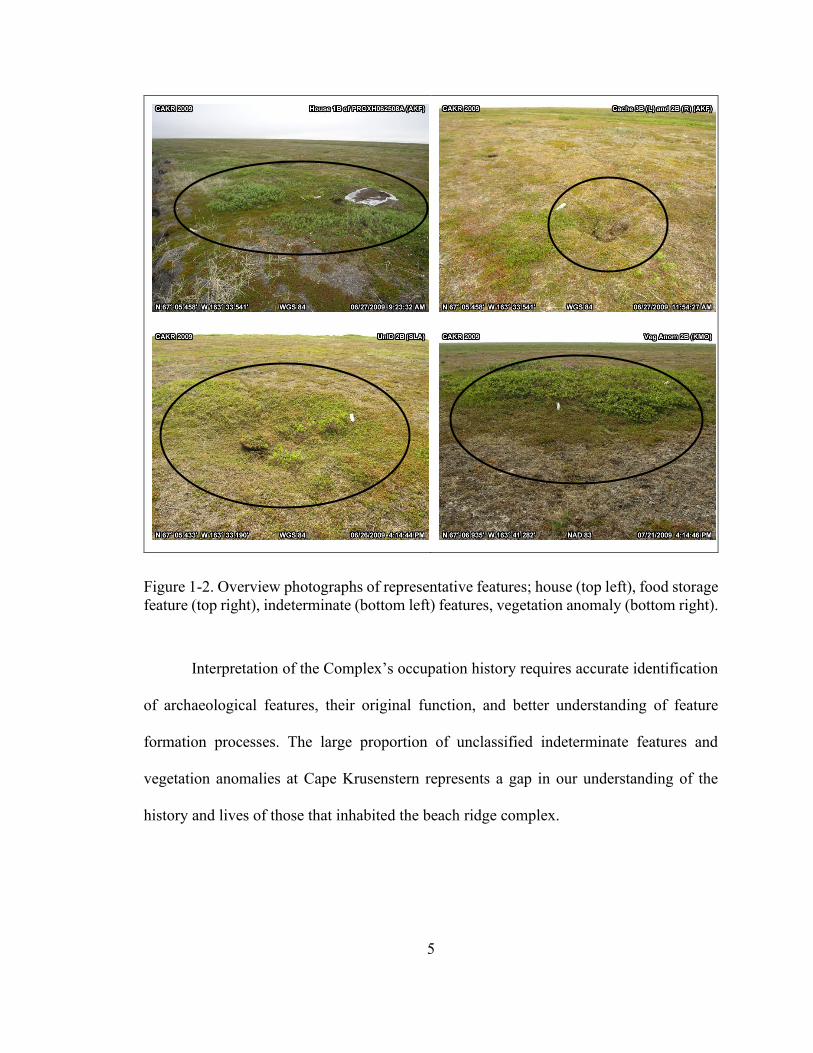
Figure 1-2. Overview photographs of representative features; house (top left), food storage
feature (top right), indeterminate (bottom left) features, vegetation anomaly (bottom right).
Interpretation of the Complex’s occupation history requires accurate identification
of archaeological features, their original function, and better understanding of feature
formation processes. The large proportion of unclassified indeterminate features and
vegetation anomalies at Cape Krusenstern represents a gap in our understanding of the
history and lives of those that inhabited the beach ridge complex.

6
Table 1-2. Feature Classifications Used in Survey of Cape Krusenstern
This thesis investigates the archaeological nature of the numerous indeterminate
features and vegetation anomalies observed at the Cape Krusenstern site complex through
multi-elemental geochemical sediment analysis. My research questions are as follows: 1)
Are the vegetation anomalies at the site complex anthropogenic or natural features? And:
2) What behaviors created the indeterminate cultural features? My analysis occurred in two
phases. In Phase I, I use photometric phosphates analysis to identify if soil phosphates are
enriched from cultural occupations. All available bulk soil samples (n=151) from features
on the first three beach ridge segments analyzed to 1) determine if vegetation anomaly is
more likely natural or anthropogenic features, and 2) to aid in selection of samples with the
most potential to contain archaeological residues created by past human activities. In Phase
II, samples tested in Phase I, along with samples from representative house and food
Feature/Sample Class Feature Description
Control Samples taken from natural areas. Measurements reflect the natural geologic
background of the beach ridge complex.
Vegetation Anomaly Vegetated areas greater than 5 m2 that are different than the surrounding
vegetation, with regular shape/appearance. May have a slight or deep
depression, or mound, within the vegetated area (~1m in depth or height). Have
the appearance of cultural features, but no cultural materials are found during
subsurface testing.
House Large surface depressions, greater than 4 m2, that may have the following
features: multiple rooms, tunnel(s), and or associated features such as cache
pits, surface scatters, or vertical posts.
Food Storage Features Small surface depressions, less than 4 m2 (when unexcavated), that may be
circular or square in shape, and are associated with a house feature or other
features.
Indeterminate Features Surface or subsurface features that contain cultural materials but do not fit in
any of the other feature categories. These are often isolated features, not found
in association with houses, activity areas, or other cultural features. They could
be the remains of a single house, a storage features associated with more
ephemeral occupations.
*Descriptions adapted from Freeburg and Anderson 2012: Appendix 1

7
storage features, were subjected to further geochemical testing. The purpose of Phase II
was threefold: (1) to collect and identify elemental concentrations and significant
patterning present in the Cape Krusenstern samples, (2) to establish distinctions between
cultural feature classes, and (3) to identify the range of human activities that created the
indeterminate features by reclassifying them as house or food storage features. The
behaviors that formed the features were identified using multi-elemental analysis. This
process involved comparing soil signatures from archaeological features of
known/interpreted function (e.g. houses and food storage features) to the soil composition
of the indeterminate features.
Theoretical Orientation
In this research, I drew on behavioral archaeological theory, particularly as it is
implemented in geoarchaeological research. Behavioral archaeology examines the
relationships between humans, their environments, and the processes that created the
archaeological materials we observe in the archaeological record (Schiffer 1972, 1975,
1976; 1987). In this case, the archaeological materials are invisible anthropogenic inputs
into sediments and soils. Behavioral archaeology complements middle range theory
building, linking human behaviors to the archaeological record. Behavioral archaeology
hinges on the concept that what is seen in the archaeological record is not a direct reflection
of the past. The archaeological record is instead the result of a series of both human (c-
transforms) and natural events (n-transforms) acting on an object, feature, or cultural
material as it transfers from its original use (systemic context) to the archaeological context
(the archaeological record) (Schiffer 1972, 1975, 1976 1987). These transforms describe a

8
variety of ways the original context, use, function, or association of an item can be
misinterpreted as it is observed in the archaeological record (Schiffer 1972, 1975, 1976,
1987). This includes past behaviors such as purposeful discard, cleanout events, and raw
material or object recycling. Additionally, natural post-depositional processes such as
erosion, feature collapse, and freeze-thaw cycles, as well as cultural processes such as
artifact collecting, and later site reoccupation and use may obscure how archaeological
materials are interpreted (Schiffer 1972, 1975, 1976, 1987).
I used behavioral archaeological theory to conduct middle range research. I
undertook geochemical analysis of soil residues to address questions about human
behaviors (e.g. food caching, domestic/house occupation) and the effect of natural
processes (e.g. decay of organic materials) on the archaeological record. My results have
implications for the reconstruction of local and regional occupation history over the last
2500 years. While the total number of features I analyzed is small, elucidation of the
archaeological nature of these features advances our understanding of the occupation
intensity at the site complex. In addition, I explored the application of a method that has
seen only limited application in Arctic settings in a new and meaningful way. Multi-
elemental geochemical analysis in archaeological studies has generally been performed at
a smaller scale, at the site or individual features level. These smaller scale studies focus on
identifying spatial patterning within archaeological features or sites, identification of site
boundaries, prospection to guide archaeological excavations, or to link specific past human
behaviors to elemental signatures (Rapp and Hill 2006:122-124: see also Couture et al.
2016 and Knudsen et al. 2010). My analysis differs by using geochemistry as a method for
feature identification at a larger landscape scale. Identifying what these features are at Cape

9
Krusenstern features could illuminate past subsistence and settlement patterns and aid in
understanding past human behaviors and site formation processes.
Thesis Organization
This thesis is organized into six chapters and three appendices. The appendices
present tables of background data as well as data resulting from the presorting and
geochemical analysis of the bulk sediment samples.
In Chapter 2, I review the geographic and prehistoric cultural context of
Northwest Alaska, focusing on previous studies of coastal settlement and subsistence
practices in northern Alaska and at Cape Krusenstern. I also review the use of soil
geochemical studies in archaeological research with a focus on prior studies that use
multi-elemental soil geochemistry to identify archaeological activity areas and features.
In Chapter 3, I present my hypotheses and expectations and introduce the
analyzed materials. I outline bulk soil sample preparation and acid digestion methods
before discussing the photometric spot test and ICP-MS multi-elemental composition
methods in greater depth. I conclude the chapter with a discussion of the statistical
methods used to compare and interpret geochemical data.
In Chapter 4, I present the results of both phases of my analysis. I highlight the
differences between control, vegetation anomaly, indeterminate feature samples, and
known feature categories before assessing the potential of reclassifying the vegetation
anomaly and indeterminate features.

10
In Chapter 5, I discuss the results of the analysis. In Chapter 6, I present the
conclusion of my research project, discuss the implications for use of ICP-MS and
geochemical multi-elemental methods, and suggest lines of further research.

11
Chapter 2 - Background
In this chapter I review the setting of the Cape Krusenstern beach ridge complex as
well as the regional prehistoric cultural context of Northwest Alaska. I focus on coastal
settlement and subsistence practices of the Thule period, including the use of house and
food storage features. I briefly present the historical development of soil geochemical
studies in archaeological research and examine recent use of multi-elemental plasma
spectrometry methods in Arctic and high latitude settings. This serves as a base for using
geochemistry as a tool to identify archaeological features, elucidate the original function,
and illuminate the past activities that created the Cape Krusenstern features in relation to
the theoretical framework of this research project.
Cape Krusenstern Beach Ridge Complex Development
Cape Krusenstern National Monument is a coastal plain with scattered brackish
lagoons and drainages backed by bluffs and upland tussock tundra hills. The shoreline that
forms the western and southern boundary of the Monument runs along the Chukchi Sea
and forms the northern entrance to Kotzebue Bay. The beach ridge complex of Cape
Krusenstern is located at the southern end of the National Monument (Figure 1-1).
The Complex is one of the oldest and most extensive beach ridge systems of the
region, forming shortly after eustatic sea levels stabilized in the Chukchi Sea approximately
5000 to 6000 years ago (Anderson et al. 2018; Mason and Jordan 1993, 2002). The beach
ridge complex is a progradational beach system comprised of sand and sandstone, chert
and limestone gravels sourced from the erosion of bedrock cliffs and bluffs along the shore
north of the complex (Hopkins 1977). These deposits were subsequently reworked by

12
longshore currents and mixed with near shelf sediments, a process that incorporated marine
shell material into the sediment. As sea levels dropped, the continued seaward formation
of new younger beaches at the active shoreline led to the initial development of barrier
islands and spit landforms, which eventually evolved into the beach ridge complex
(Anderson et al. 2018; Hopkins 1977). The more than 100 beach ridges at the Complex
serve as horizontal stratigraphy linking the development of the Complex to past human
occupations and environmental conditions (Anderson et al. 2018; Anderson and Freeburg
2013, 2014; Freeburg and Anderson 2012). The oldest beach ridges, and the oldest human
occupations, are located on the north side of the Complex, while younger ridges and
occupations are found closer to the modern shoreline. The beach ridge segments serve as a
proxy for past coastal processes and provide a temporal framework for human occupation
of the Complex. Early development of the beach ridge complex appears to have been
relatively rapid and consistent between 5000 and 3000 cal. BP. This is indicated by the
broad form and low elevation of ridges on segments IV and V, suggesting a period of
relatively stable climate; sediment supply to the complex was potentially low during this
period. After 2100 cal. BP numerous truncations and orientation shifts in the beach ridges
suggest a period of increased climatic variability (Anderson et al. 2018; Mason and Ludwig
1990; Mason et al. 1995). The younger beach ridges are smaller in width, with more
variable form, and have a higher maximum elevation. The difference in ridge form may be
indicative of increased sediment loads and more intensive coastal processes during the later
periods (Anderson et al. 2018).

13
Current Interpretation of Coastal Hunter-Gatherer Settlement Patterns in Northwest
Alaska
Early research at Cape Krusenstern, conducted by J. Louis Giddings and Douglas
D. Anderson, established that people occupied the Complex shortly after its formation and
continued to utilize the area into the present day (Giddings and Anderson 1986). The
earliest preserved human use of Arctic Alaskan coastal areas (4500 BP to 2800 BP) was
limited to seasonal use by small, highly mobile groups, with a broad subsistence base. More
intensive use of coastal environments, derived from the presence of higher investment
semi-subterranean house features and larger settlements, is evident in northern Alaska
starting around 2800 BP. Beginning approximately 2000 years ago, dramatic increases in
population, settlement size, and the number of semi-subterranean houses, plus the
expansion of social complexity, are apparent around the region(Anderson 1984; Anderson
and Freeburg 2014; Anderson et al. 2018; Freeburg and Anderson 2012; Giddings and
Anderson 1986; Mason 1998). Around 1350 BP, the Birnirk people, predecessors to the
Thule peoples, appear along the coasts of the northern Arctic from the Bering Strait to the
North Slope. The presence of whale bone in faunal assemblages (i.e. its use in house
structures and other cultural materials) is interpreted as evidence of whaling during this
period (Mason 2000; Mason and Barber 2003). The development of the Thule from the
Birnirk occurred sometime between 1200-950 years BP (Anderson 1984; Giddings and
Anderson 1986; Mason 2000). As Thule culture developed, Thule people spread rapidly
across the North American Arctic, bringing with them a specialized maritime hunting
technology (e.g. multicomponent harpoons) and an increased focus on marine resource use
(Anderson 1984; Giddings and Anderson 1986). Considerable variability in technology,
14
subsistence practices, and social complexity is represented in larger multi-family houses
and community structures occurring throughout this period (Anderson 1984; Giddings and
Anderson 1986).
Cape Krusenstern Features and Population Dynamics
At Cape Krusenstern, there is an increase in anthropogenic archaeological features
during the period between 1750 BP and 1150 BP, including semi-subterranean houses and
food storage features. This increase in the number of features suggests intensified
occupation, population increases, and specialized food processing and storage activities at
the beach ridge complex (Anderson and Freeburg 2013, 2014; Anderson et. al 2018;
Freeburg and Anderson 2012). The Thule period is marked by three major declines in
population: approximately 1250-1000 BP, 850-750 BP, and 750-450 BP. These declines
are identified by a relative lack and or lower quantity of features dating to those periods
(Table 1-1) (see Figure 8: Anderson et al. 2019; Anderson and Freeburg 2014; Anderson
et al. 2018; Freeburg and Anderson 2012; Giddings and Anderson 1986). Giddings and
Anderson (1986) note that Thule peoples continued a semi-sedentary lifestyle and shifted
their subsistence practices from marine mammal hunting to more intensive fishing. Some
researchers have attributed these decreases in settlement sizes and occupational intensity
to the dispersion of Thule peoples around the coast and migrations into the interior as
responses to increasing population pressures and resource competition (Gerlach and Mason
1992; Mason 1998; Mason and Barber 2003). Starting 500 years ago, the archaeological
record indicates a continued decrease in settlement size and further dispersion of

15
occupations into previously unoccupied areas of the coast and interior river valleys
(Anderson et al. 2019; Junge 2017).
In Northwest Alaska, the presence and quantities of semi-subterranean houses and
food storage features are used as the basis of population estimates and indicators of
increased sedentism and intensification of resource use ( Anderson and Freeburg 2014;
Anderson et al 2019; Dumond 1975; Giddings and Anderson 1986; Mason 1998); this is
similar to hunter-gatherer practices in other parts of the world (.e.g Ames 1994). Measures
of occupation intensity have relied on the density of archaeological features, such as house
and storage features, to establish estimates of population. House features in particular,
paired with ethnographically informed assumptions about the number of occupants per
house (Burch 1984:316-317, 1998:20), are used as general baselines for population
estimates (e.g. Mason 1998). Additionally, archaeological features such as storage features
and evidence of resource caching and marine resource use are linked in many cases to the
development of larger populations, increased sedentism, technological complexity, and in
some cases, the emergence of social complexity (Ames 1994; Anderson and Freeburg
2014; Erlandson 2001; Fitzhugh 2003).
While feature counts are a primary source of archaeological information, using
them to estimate population can be problematic for numerous reasons (Chamberlain
2006:126-132). Namely, it is hard to say without extensive supporting excavations and
analysis such as radiocarbon dating whether a house or series of houses was occupied at
the same time, consecutively by a single family returning yearly, or concurrently by several
families (Hassan 1978; Ropper 1979). Additionally, the use of storage feature quantities
alone is problematic as many storage features may be associated with a specific/singular

16
occupation. This is compounded by the fact that multiple storage feature types (i.e. for
different resources) were likely in use at a single time. Therefore, it is important that
archaeologists understand the context of feature types present in the archaeological record
(Chamberlain 2006: 126-132; Schiffer 1976). Geochemistry can provide information
regarding archaeological feature types in order to develop the context necessary to
accurately interpret their function, as well as guide future research to date them and identify
similar features. The identification of more features and their function can provide
additional information to better understand the cause of declines in population at the
Complex.
Thule Sites: Houses, Storage Features, and Activity Areas
Arctic semi-subterranean house structures have been well documented both
ethnographically and archaeologically since the early 20th century. Houses are highly
variable in form at a regional level. Construction materials and internal arrangement are
tied to distinct cultural groups and periods, as well as representing social practices or
institutions (e.g. whaling crews, increasing social complexity), and/or different functional
or seasonal uses of houses (Darwent et al. 2013; Dussault 2014; Giddings and Anderson
1986; McGhee 1984; Norman et al. 2017; Park 1988). Regional work including at the
Complex and Cape Espenberg, located southwest of the Complex across Kotzebue Sound
(Figure 1-1), has helped shed light on the internal arrangement and use of space in semi-
subterranean houses and, more specifically, those of the Thule house (Braymer-Hayes
2018; Norman et al. 2017; Norman 2018). The following discussion serves to describe the

17
form and variety of activities performed in Arctic semi-subterranean houses, storage
features, and activity areas that may be reflected in geochemical residues.
The typical Thule winter house form consists of a single main room where most
daily activities would have taken place. The main room is accessed and protected from the
outside by way of a long sunken entrance tunnel that served as a cold trap. Separate rooms
or alcoves, often thought to be cooking rooms or kitchen areas, are common features,
especially in later Thule houses. Kitchen areas are generally well defined by midden
deposits associated with burnt marine mammal oils, crushed bone, and charcoal. Internal
central hearths were not a common feature of early Thule houses, in which lighting and
heat primarily came from the use of local ceramic or soapstone oil lamps (Norman et al.
2017; Park 1988, 1999). The sides of many houses contain elevated split log benches along
the internal walls of the main room. These benches often functioned as sleeping platforms,
lamp stands, as well as occasional internal storage. Structural architecture of the houses is
primarily driftwood log posts and/or whale bone, and floors are formed from split wood
logs (Alix 2005, 2016). The use of both skins and sods as insulating layers to form the
major exterior wall and roof segments has been reported (Alix 2005, 2016; Park 1988,
1999).
Layers of cultural deposits have been found in the areas of tunnels, suggesting the
deposition of internal cleaning episodes (Norman et al. 2017; Park 1988, 1999). Cemented
sediments are often observed below the floorboards and less often reported at various
places around the perimeter of the main room. The cementation is believed to be caused by
the conglomeration of sediments by marine mammal oils, either from spillage of oil lamps

18
or, as has been suggested, as potentially intentional in some areas, likely serving as a means
of sealing the sediments of the perimeter (Norman et al. 2017; Norman 2018; Park 1988).
As discussed previously, Thule culture is characterized as having a highly adept
maritime focused subsistence, with technology adapted for intensive hunting of marine
mammals, the associated environmental conditions, and high group mobility. The highly
specialized marine mammal hunting technology (e.g. composite harpoons, skin boats and
skin floats) allowed people to take larger game, providing greater quantities of resources
(Giddings and Anderson 1986; Mason and Barber 2003). This necessitated methods of
processing and food dispersion to save food for later use without spoiling (Giddings and
Anderson 1986; Park 1988; Sheehan 1995). Ethnographically, the use of external cache
pits (here, food storage features) on the coast is generally tied to seal and marine mammal
products after harvesting and processing. Often the primary harvest and processing of large
marine mammals occurred in spring and summer on active beaches with only flesh,
blubber, skin, and limited bones being taken to inshore locations for hang drying and
preservation for winter consumption (Giddings and Anderson 1986:319; Park; 1988;
1999). Blubber was often placed in seal skin bags, or pokes, and dried meats were similarly
stored in skin bags and placed in stone or dug out pit caches (Burch 1998:53; Park 1988,
1999).
The construction of cache pits has seen relatively limited research in Arctic studies.
This is likely due to their simple construction which can lack architectural elements.
Ethnographically, caches are constructed as stone or wood dug-out pits, and often lined
with vegetation such as seaweeds and capped by rocks or log covers to prevent predator
scavenging (Burch 1998:53, 73, 298; Entwistle 2007; Park 1988, 1999). Above-ground

19
wood built caches are also noted at village locations (Burch 1998:185). The location of the
pits in relation to living structures has also seen limited research in archaeology, though
ethnographic accounts indicate caches would be placed near the site of processing (similar
to interior terrestrial mammal meat processing) or adjacent to village and house locations
(Park 1988, 1999). However, evidence of processing or temporary storage of foods taken
in winter, either on the ice or when covered by snow, would not likely preserve.
Geochemical analysis of soil residues may elucidate the subsistence practices of the Thule
people in relation to the development and use of food resource storage pits.
Geochemical Analysis of Soils in Arctic or Subarctic Settings as a Tool for
Identification of Archaeological Features
Above I discuss Thule house construction, subsistence, and resource caching as
discrete archaeological features that may be found in the archaeological record and are
suggestive of past human behaviors. However, decomposition and use may obscure or
remove the visible traces of these features and activities from the archaeological record.
These past behaviors have implications for how these features may be expressed in the
geochemical archaeological record.
Soil geochemistry has been utilized as a tool in archaeological investigation since
the early 20th century (See Arrhenius 1929; 1962; and 1954: Lorch 1939). Early research
observed increased levels of calcium (Ca), carbon (C), nitrogen (N), and phosphorus (P) in
soils as indicators of past human presence at those locations. These elements are tied to the
human deposition and decomposition of organic materials and refuse such as Ca from bone
and shell, C from charcoal and general decomposition of organic materials for N and P.

20
Phosphate analysis became the dominant method, as anthropogenic or organic P is
recognized as being easily separated from naturally occurring soil phosphorous (Barba
2007; Eidt 1977; Heizer and Cook 1965; Lutz 1951; Middleton and Price 1996; Rypkema
et al. 2007). Numerous test methods exist for in-field and laboratory geochemical elemental
analysis. However, many are purely qualitative, possess limited precision, focus on single
elements and minerals, or are primarily utilized to guide archaeological prospection and
excavations (Eidt 1977; Holliday and Gartner 2007; Middleton and Price 1996). With the
advent of mass spectrometry (the sorting of ions of elements based on their mass to charge
ratio), the field of archaeological geochemistry has turned to using multiple elements as
indicators of human presence. Inductively coupled plasma mass spectrometry (ICP-MS)
and inductively coupled plasma atomic emission spectrometry (ICP-AES) are the most
common methods for soil geochemical analysis because they can analyze multiple
elements and provide reliable quantitative data for analysis at a relatively low cost.
Research utilizing multi-element analytical methods is increasing in the region and
improving our understanding of how anthropogenic activities influence soils.
Numerous archaeological and ethnoarchaeological geochemical analyses have
established that geochemical analysis works well in Arctic soil depositional environments
(Buonasera et al. 2015; Couture et al. 2016; Hoffman 2002; Knudson et al. 2004; Knudson
and Frink 2010; Lutz 1951). More specifically, many studies have provided information
about potential sources of elemental soil inputs (Butler 2008; Goffer 2007; Heizer and
Cook 1965; Misarti 2007; Oonk et al 2009; Wells 2004a). These studies established that in
addition to P and Ca, other elements including sodium (Na), potassium (K), aluminum (Al),
manganese (Mn), magnesium (Mg), barium (Ba), strontium (Sr), titanium (Ti), zinc (Zn),

21
and iron (Fe) often appear in either elevated or depleted concentrations as a result of
specific human activities (Table 2-1). In particular, Misarti et al. (2011) found significant
distinctions between anthropogenic sediments and natural sediments in the concentrations
of Fe, Ti, P, Sr, and Zn levels from two Aleutian Islands archaeological sites. Statistical
analysis of the element concentrations showed house pits and midden deposits were easily
distinguished from each other and from other “on site” soils (Misarti et al. 2011).
Geochemical analysis has great potential to identify the types of signatures that may
characterize Arctic house features. Couture et al. (2016) used soil geochemical analysis
and micromorphology to study spatial patterning of 18th century Inuit houses in northern
Labrador. The elemental enrichment patterning indicated the influence of past behaviors
and activities on specific locations within houses (Table 2-1). Specifically, floors and
entrance tunnels showed similar enrichments of the same elements and compounds (P, Sr,
and CaO), while sleeping platforms had unique signatures with additional enrichment of
organic Ba and Na2O. Marine mammal oil lamp maintenance was tied to the enrichment
of S and Zn present on lamp stands or alcoves. Overall, this study shows the potential of
identifying internal spatial patterning from geochemical analysis. Statistically, however,
the distinctions were generally only clear in two of the houses. The incongruence seen
between houses may be indicate depositional processes in the systemic context, such as the
mixing of deposits from different areas from multiple cleaning events.
22
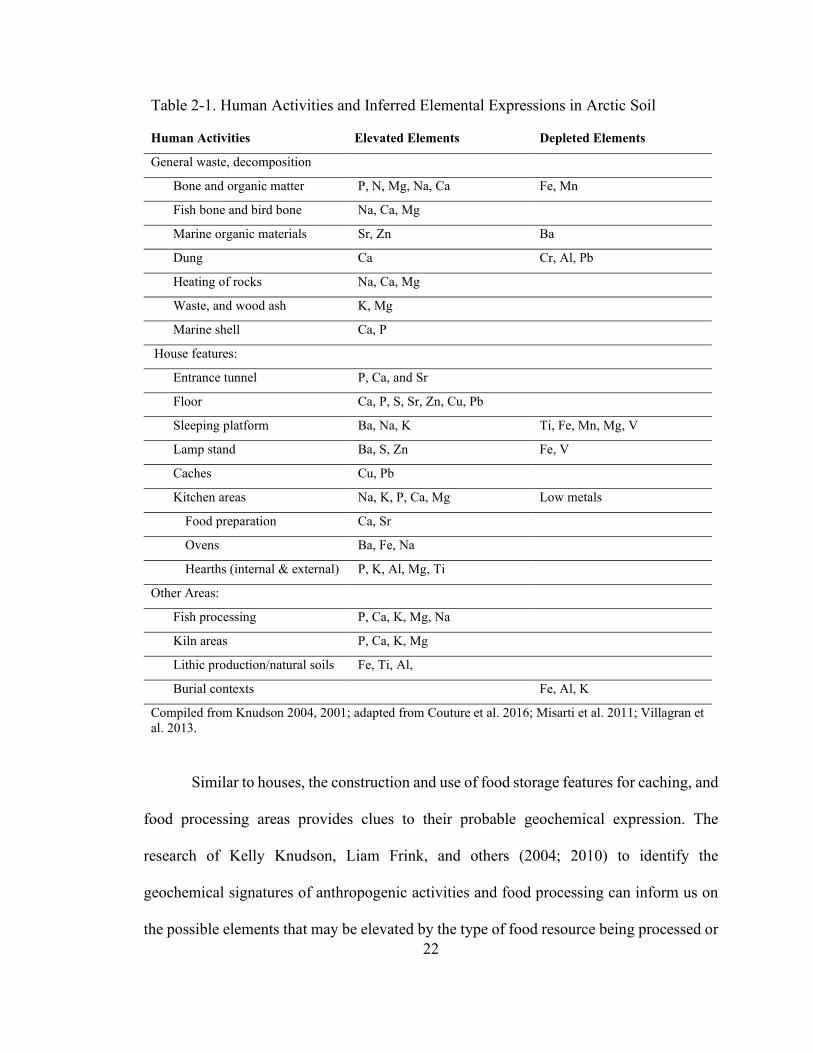
Similar to houses, the construction and use of food storage features for caching, and
food processing areas provides clues to their probable geochemical expression. The
research of Kelly Knudson, Liam Frink, and others (2004; 2010) to identify the
geochemical signatures of anthropogenic activities and food processing can inform us on
the possible elements that may be elevated by the type of food resource being processed or
Table 2-1. Human Activities and Inferred Elemental Expressions in Arctic Soil
Human Activities Elevated Elements Depleted Elements
General waste, decomposition
Bone and organic matter P, N, Mg, Na, Ca Fe, Mn
Fish bone and bird bone Na, Ca, Mg
Marine organic materials Sr, Zn Ba
Dung Ca Cr, Al, Pb
Heating of rocks Na, Ca, Mg
Waste, and wood ash K, Mg
Marine shell Ca, P
House features:
Entrance tunnel P, Ca, and Sr
Floor Ca, P, S, Sr, Zn, Cu, Pb
Sleeping platform Ba, Na, K Ti, Fe, Mn, Mg, V
Lamp stand Ba, S, Zn Fe, V
Caches Cu, Pb
Kitchen areas Na, K, P, Ca, Mg Low metals
Food preparation Ca, Sr
Ovens Ba, Fe, Na
Hearths (internal & external) P, K, Al, Mg, Ti
Other Areas:
Fish processing P, Ca, K, Mg, Na
Kiln areas P, Ca, K, Mg
Lithic production/natural soils Fe, Ti, Al,
Burial contexts
Fe, Al, K
Compiled from Knudson 2004, 2001; adapted from Couture et al. 2016; Misarti et al. 2011; Villagran et
al. 2013.

23
stored. Using ICP-AES, they found elevated levels of Ca, P, Na, and Sr in soils from inside
the boundaries of known fish drying racks. The elevated elements are attributed to the
decay of bones and accumulated oily drippings in the soil over the use life of the drying
rack (Knudson et al. 2004). Additional ethnoarchaeological contexts of herring processing
camps and activity areas on Nelson Island in western Alaska were analyzed using ICP-MS
(Knudson and Frink 2010). The analysis indicated similar elevation levels of Na, Mg, Mn,
Al, P, K, Fe, cobalt (Co), copper (Cu), and lead (Pb) in the tested features. Ratios of Ba/Ca
and Sr/Ca concentrations are noted as depleted in fish processing areas (Knudson and Frink
2010; Knudson et al. 2004). These element ratios are used as indicators for marine
influence on archaeological soils (Burton and Price 1990; 1999; Knudson et al. 2004;
Knudson and Frink 2010). Ratios of these elements are inversely tied to trophic levels,
decreasing as trophic levels increase (Burton and Price 1999; Knudson and Frink 2010).
Maschner et al. (2010:71-77) had similar results with multi-elemental geochemical
analysis on soils from two archaeological sites along the Sapsuk River in western Alaska.
Couture et al. (2016) similarly found that caches were enriched in Cu and Pb.
Geochemical Analysis of Soils as a Tool for Identification of Marine and Terrestrial
Food Resources
Work outside of Alaskan archaeology has also contributed to our interpretations of
the elemental inputs that various animal types have on archaeological soils and sediments.
Villigran et al. (2013) conducted multi-elemental geochemical analysis alongside micro-
morphological and fatty acid analysis of sediments from two sealing structures in
Antarctica. The authors found elevated levels of P2O5, CaO, Zn, and Cl and depleted levels

24
of SiO, Al2O3, and Fe2O3 in a combustion feature. The elevated values are attributed to the
presence of seal remains, including burnt seal bone and charred material, as Cl is elevated
in seal soft tissue. Villigran et al.’s (2013) interpretations of soil element and mineral
composition were informed by food and nutritional sciences research showing that the
blubber and meat of Greenlandic harp (Pagophilus, or Phoca, groenlandica) and hooded
seals (Cystophora cristata) have high values of dietary minerals (e.g. major elements Ca,
P, K, Na, and Mg; and trace elements S, Fe, Cl, Co, Cu, Zn, Mn, molybdenum (Mo), iodine
(I), and selenium (Se)), though Ca and Fe are particularly high (Synowiecki 1993;
Brunborg et al. 2006). Similar values of Ca, Fe, Zn, and Mg are found in other marine
mammal species important to western Arctic Alaskan diets, such as bearded seals
(Erignathus barbatus), ringed seals (Pusa hispida), and walrus (Odobenus rosmarus)
(Kuhnlein et al. 2002). Additionally, beluga (Delphinapterus leucas) and narwhal
(Monodon monoceros) show little elemental distinction between each other and from other
marine mammals. However, high Se values are observed in raw beluga and narwhal
muktuk, as well as walrus meat (Kuhnlein et al. 2002). Villagran’s study also found
elevated levels of sulfur (S) in samples associated with fur and skin materials in the
sediment matrix. This is corroborated by Gillespie and Frenkel (1974), who indicated that
seal fur keratin is high in S compounds. Villigran et al. (2013) also noted high Fe levels in
sediments with high fatty acid content which is interpreted as a signature for seal blood
(Brunborg et al. 2006; Shahidi and Synowiecki 1993; Yamamotto, 1987). This research
suggests that Cl, S, and Fe may serve as indicators for food storage feature contents as
these are where items such as seal skin pokes may have been stored. Additionally, as
marine mammal skin use was ubiquitous across the Arctic (Burch 1998), the signature

25
could potentially be linked to other aspects of archaeological features such as roof
coverings or bedding materials in houses.
While there is considerable nutritional research on seals, less information is
available for other important food sources, such as terrestrial mammals. A study by Butler
et al. (2013) showed elevated concentrations of K2O, MgO, Fe2O3, Sr, Sc, Y, Ca, Ni, and
Pb in areas where open air animal processing is thought to have occurred. This research
from the central Canadian Arctic is corroborated by the use of fourier transform infrared
spectroscopy (FTIR), which showed the presence of trans-fats associated with ruminant
tissues, interpreted to be caribou, preserved in the sediments. Kuhnlein et al.’s (2002) arctic
dietary research also included many Arctic terrestrial mammals (see Table 3 in Kuhnlein
et al. 2002:554-557). The authors showed that mineral compositions in terrestrial mammals
are generally low (except in P, Mn, and K, which are similar to other animals) when
compared to marine mammals.
Non-Human Influences and Natural Process on Sediment Elemental Concentrations
There is considerable research that establishes humans as the agent of elemental
enrichment in sediments as a result of the deposition and decomposition of organic
materials, including bodily wastes (Burton and Price 1990; Couture et al. 2016; Lutz 1951;
Misarti 2007). However, there is little research to establish if a distinction between human
and non-human enrichment is possible. That is, do animals (such as Arctic fox {Vulpes
lagopus}) create different soil signatures than humans, and can this be used to identify
anthropogenic versus natural features on the landscape? This question is of interest in the
Arctic where sediment accumulation and soil formation are slow, and animals like the

26
Arctic fox and ground squirrel (Spermophilus parryii), which build dens, can create
features on the landscape that mound and have high vegetative potential like those of past
human occupations.
Some researchers, such as Misarti et al. (2011), cite sediment and plant nutritional
research that suggests that the presence of fox on landscapes results in significant decreases
in N and P availability in natural soils (Croll et al. 2005; Maron et al. 2006), though
Misarti’s results did not actually show the predicted decrease in N and P. The assumption
made by the cited research (Croll et al. 2005; Maron et al. 2006) is reliant upon a multi-
trophic level relationship between fox predation and marine birds, whose excrement is the
major supply of the soil nutrients. Unfortunately, this is not a direct measure of fox
influence on landscapes, and presumably a human presence on a landscape could have the
same effect. Gharajehdaghipour et al. (2016) specifically tested the nutrient availability of
Arctic fox dens and showed dramatic increases of inorganic N and P. These increases,
however, are highly variable and fluctuate seasonally, presumably due to the intensity of
litter/pup rearing and the intensity of urine, feces, and food waste accumulation. This
research has implications for interpreting features based purely on common soil nutrient
minerals such as N and P, where burrowing animals may have affected or contributed to
the geochemical signature.
Limitations of Geochemical Analysis and Identifying Features and Function
Geochemical analysis has two major limitations relevant to this study. First, while
elemental enrichment and depletion levels are useful for detecting anthropogenic
phenomena, elemental data alone does not provide a complete picture of the past, and

27
accompanying analyses (i.e. micromorphology, detailed excavation) are required to fully
contextualize geochemical findings for meaningful archaeological interpretation. This
limits the level at which interpretation can be made in identifying the specific past event,
behavior, or item that created the signature. While research suggests that distinctions
between features types (e.g. house versus caches) is possible, geochemical studies alone
are not sufficient to determine the specific species people were processing or storing in
features. However, in conjunction with other data on cultural behavior (e.g. feature form)
and analyses (e.g. aDNA, or soil lipids) it is possible to generate more broad information
regarding food contents as marine versus terrestrial mammal use (Knudsen et al. 2004;
Knudson and Frink 2010), or internal spatial distinctions (Couture et al. 2016); this is
minimally a greater level of detail than what could be said with limited excavation in
features where physical materials (i.e. bone or structural materials) have not preserved.
Second, this limitation is further compounded by the need for a deep understanding
on the effects that weathering and other post-depositional processes such as diagenesis,
cryoturbation, etc. can have on the potential chemical properties of sediments and soils.
This understanding is necessary to account for the observations and interpretations of
elemental concentrations. This limitation is more easily overcome by understanding the
geochemistry of local native sediments and having a robust set of natural non-cultural
control samples provides a baseline to asses any potential affect that post depositional and
or weathering processes may have.

28
Chapter 3 - Materials and Methods
In Chapter 3 I discuss the materials and methods used in this study. First, I present
the hypothesis and expectations of my research project. I then consider the Cape
Krusenstern bulk sample collections and the sample selection process. I introduce the
methods I use for bulk soil sample preparation and acid digestion methods. I then discuss
the Phase I soil spot tests and Phase II ICP-MS elemental composition methods. I conclude
with a discussion of the statistical methods I use to compare and interpret the geochemical
data.
Hypothesis and Expectations
My research addresses two question: 1) Are the vegetation anomalies at the site
complex natural or anthropogenic features? And: 2) What behaviors created the
indeterminate cultural features? Addressing these questions required a two-phase approach
(Table 3-1).
The primary goal of Phase I was to determine if the vast number of vegetation
anomaly features present at the complex actually represent a large unidentified
anthropogenic component of the archaeological record. Unfortunately, as the vegetation
anomalies did not contain archaeological materials, only a single feature was sampled in
the field. I tested multiple samples from Vegetation Anomaly 3624B (samples; CAKR
14172-14176) to assess if the vegetation anomaly feature class are likely a natural or
cultural feature. To do this, I compared vegetation anomaly samples to natural control
samples and to samples from known cultural features (specifically houses). Phase I had an
additional implication for Phase II of my analysis; that is, identifying which samples had

29
the highest concentrations of phosphates, and thus the greatest potential to contain
archaeological residues. I use these samples in Phase II.
Null Hypothesis (H-10): If the level of phosphorus in the vegetation anomaly samples are
not elevated, or are at similar concentrations in comparison to control samples, then
Vegetation Anomaly 3624B is likely a natural feature.
Hypothesis 1 (H-11): If levels of phosphorous in the vegetation anomaly samples are a)
observed as elevated in comparison to control samples and b) at similar levels to house and
food storage features, Vegetation Anomaly 3624B is likely anthropogenic and will be
reclassified as an indeterminate feature. Samples from this feature are used regardless of
phosphate testing results for further analysis in Phase II testing Hypothesis 2.
Table 3-1. Hypotheses, Expectations, and Analytical Methods
Hypothesis Description Expectation Analysis Method
H-10: Vegetation anomaly is a
natural feature
Similar phosphate levels to
control samples
Phosphates Spot
tests
H-11: Vegetation anomaly is
anthropogenic
Elevated phosphate levels
indicate anthropogenic
Phosphate spot tests
H-20: House and food storage
features are indistinguishable.
Indistinct elemental
concentrations
ICP-MS
H-21: House and food storage
features have distinct
geochemical signatures
Distinct elemental
concentrations
ICP-MS
2a: Indeterminate features are
houses
Element concentrations
group with houses
ICP-MS
2b: Indeterminate features are
food storage features
Element concentrations
group with food storage
features
ICP-MS
H-30: Food storage features have
indistinguishable geochemical
signatures
Distinct elemental grouping
within food storage features
ICP-MS
H-31: Food storage features have
multiple distinct geochemical
signatures
Distinct elemental grouping
within food storage features
ICP-MS

30
The goal of the second phase of my analysis was to identify the past behaviors that
created the indeterminate features, i.e. whether the indeterminate features were occupation
features (i.e. houses) or food caching features (i.e. food storage features). In Phase II, I
establish that differences between house and food storage features exists (H-21 and H-20),
and I then compare the elemental concentrations of the indeterminate features to the
elemental concentrations of control samples and features of known function (house and
food storage features).
Null Hypothesis (H-20): The cultural features will not have distinctions in elemental
composition based on use and past activities that created them. The cultural features are
not geochemically distinguishable between each other and the elemental signatures are
reflective of general anthropogenic activities. I compare house and food storage feature
samples to evaluate this hypothesis.
Hypothesis 2 (H-21): The cultural features will have distinctions in elemental composition
based on use and past activities that created them. The house and food storage features are
geochemically distinguishable between each other and the elemental signatures are
reflective of the anthropogenic activities that created them. Indeterminate features are
similar to house or food storage feature signatures. I compare cultural feature samples to
evaluate this hypothesis and explore the nature of the indeterminate features by the sub-
hypotheses below.
Hypothesis 2a: The indeterminate features are houses. House deposits have a broad range
of elevated or depleted elements within the soils, reflecting the wider range of daily
activities that took place within the house structure. Specifically, food preparation and

31
consumption will elevate levels of Ca and Sr if small bones are discarded and the use of
seal oil lamps and ash from cooking fires will elevate Ba, Fe, Na, K, P and Mg (Middleton
and Price 1996). Decomposition of plant and animal materials such as hides and bone
implements will elevate Ca, K, Mg, Na, and P in soils (Table 2-1; Entwistle et al. 1998;
Entwistle et al. 2000; Middleton and Price 1996). There are a variety of potential elemental
enrichment patterns that could be expressed in house features and the signatures of houses
are not limited to those discussed here. I compare indeterminate feature samples to house
feature samples to evaluate this hypothesis.
Hypothesis 2b: The indeterminate features are food storage features. Food storage features
will have fewer elements at elevated or depleted levels in comparison to house features.
This chemical composition reflects the more limited use or activities related to storage
features in comparison to occupation features. In particular, decomposition of plant
materials from pit linings, and animal/food material contents will elevate Ca, K, Mg, Na,
Cu and Pb and P in as well as deplete Fe and Mn soils (Table 2-1; Entwistle 2007;
Middleton and Price 1996). I compare indeterminate feature samples to food storage
feature samples to evaluate this hypothesis.
After I identify probable new food storage features, I then assess the potential of
identifying the stored contents of the food storage features.
Null Hypothesis 3 (H-30): If the food storage features (including reclassified
indeterminates) do not represent distinct storage features related to the contents of that
feature, then the geochemical signatures will be similar to each other, and no distinctions
between the features can be made.

32
Hypothesis 3 (H-31): If the food storage features were used to store different materials, the
specific elements that are elevated or depleted within food storage feature samples will
reflect the contents of that feature. Fish remains have been shown to elevate Ca, P, Na, and
Sr levels in soil, and to deplete Ba levels (Knudson and Frink 2010; Middleton and Price
1996; Misarti et al. 2011). I compare the specific patterning between food storage feature
samples (including reclassified indeterminate feature samples) to evaluate this hypothesis.
Materials
I analyze a 151-sample subset of the 230 bulk sediment samples collected from
Cape Krusenstern between 2008 and 2010 (Freeburg and Anderson 2012). As a field crew
member for the project in 2008 and 2009, I participated in the collection and field
processing of these bulk samples. The bulk samples I analyze are from the first three beach
ridge segments and represent 39 unique feature locations associated with houses (n=7
features; 36 samples), food storage features (n=4 features; 23 samples), indeterminate
features (n=27 features; 87 samples), and vegetation anomalies (n=1 features; 5 samples)
from the Thule occupation of the site complex (Figure 3-1; Table 3-2; Appendix A Table
A-1). Samples from features that were designated in the field as house and food storage
features are used as cultural controls in this analysis. Samples came from a variety of
contexts and features encountered during the archaeological investigations. Generally, bulk
samples were collected from shovel tests and excavation units either in arbitrary 10 cm
levels or natural levels when identified in the field. Not all features were sampled at the
same regular intervals or to the same depth and some sampling occurred only in cultural
deposits. Some samples represent replicate and or duplicate sample elevations from the

33
features; these samples are included in Phase 1 analysis to address any potential post-
collection biases introduced by splitting bulk samples (replicate) or sample collection
location (duplicate). Control samples (n=1 locus; 8 samples) were also collected from
presumed non-cultural deposits (areas removed from feature locations and where no
surface or subsurface archaeological materials had been identified). Bulk samples collected
from 2008 and 2009 were not screened in the field, while bulk samples collected in 2010
were screened through 0.25-inch mesh in the field to reduce packing weight and to identify
any small artifacts that were present. Additional sorting of the 2008 and 2009 collected
materials occurred in lab to reduce the bulk, and sediment materials were separated into
multiple size fractions down to 1mm (.039 inches). Additional control samples (n=4) were
collected from four unique locations in the summer of 2017 by NPS archaeologist Andrew
Tremayne.
Table 3-2. Features and Samples used in Analysis
Beach Ridge Segment
Feature Class:
Feature Quantity
(Number of Samples)
I
II
III
Total
Cu
ltu
ral
Fea
ture
s
Houses 3 (15) 4 (21) - 7 (36)
Food Storage Features 4 (23) - - 4 (23)
Indeterminate Features 3 (17) 25 (68) 1(2) 28 (87)
Nat
ura
l Vegetation Anomalies - 1 (5) - 1 (5)
Controls 1 (8) 4(4) - 5 (12)
Total 11(63) 31(98) 1(2) 44
(163)

34
Fig
ure
3-1
. S
ample
and f
eatu
re l
oca
tions
by f
eatu
re c
lass
.

35
Geochemical Methods
The use of geochemical analysis to identify anthropogenic indicators in
archaeological sediments has stirred much debate regarding appropriate digestion methods.
It is possible that acid digestion procedures may be too strong and hide anthropogenic
inputs in geologic backgrounds, or conversely too weak and unable to fully digest the
anthropogenic inputs. Many studies attempted to address these methodological issues,
however, there is little consensus regarding the best method to capture anthropogenic
residues (see Knudsen and Frink 2010; Wells 2010; Wilson et al. 2006).
One study, Wilson et al. 2006, looked at the distinction between two methods, a
strong acid dissolution versus a five-step sequential digestion. The results of the study
suggested that the use of weak acid digestion method could result in the loss of information
regarding anthropogenic inputs, but the study concluded that the choice of extraction
method is ultimately element and soil specific (Wilson et al. 2006:443). The authors
suggest that a pseudo-total extraction method such as HNO3 strong acid digestion is a
suitable method to identify such interactions and any issues that would warrant the use of
element specific extraction methods.
Despite this, a majority of archaeological chemical studies in the Arctic (see
Knudson and Frink. 2010; Wells 2010; Wilson et al. 2006) have placed an emphasis on the
use of weak or mild acid extraction methods, commonly an open digestion with a mixture
of HCl. The basis of this digestion method is to digest what are believed to be more mobile
elemental sediments and soil inputs which are assumed to reflect anthropogenic additions
rather than fully digest geologic background signatures. This digestion method has shown

36
to give reliable results, and has been used across both ICP-AES/OES and ICP-MS. I elected
to use this method in my analysis based on its relative simplicity of execution and for
regional comparison.
Phase I Method: Photometric Spot Tests
In Phase I, I selected 151 sediment samples of the total 230 collected samples from
the first three beach ridge segments. I selected samples from known feature classes,
indeterminate features, and the vegetation anomaly, as well as control samples from
independent locations presumed to be non-cultural (Appendix A; Table A-1). Controls
were considered to be from non-cultural contexts and representative of natural sediments
as they did not react for phosphates in Phase 1. Initial sample preparation included air
drying as necessary for 24-48 hours before being sifted through 0.25 inch (6.35 mm), 0.125
inch (3.175 mm), 0.078 inch (2 mm), and 0.039 inch (1 mm) graduated sieves to remove
large constituents and identify any cultural materials (i.e. debitage, bone, wood). I use the
fine < 1mm fraction in my analysis as sand size materials are necessary and allow for
comparability in results to the geochemical methods I selected to use (Barba et al. 1991;
Knudson et al. 2004; Knudson and Frink 2010; Middleton and Price 1996; Wells 2010;
Wilson et al. 2006. The samples were then subsampled by weight as required for the soil
composition tests (between 0.05 g and 0.20 g per sample).
After initial sample preparation, I performed a series of simple chemical procedures
(spot tests) to identify the presence of soil phosphates. Spot tests are an inexpensive and
simple first step to assess anthropogenic soil inputs. These spot tests utilize methods set
forth by Luis Barba et al. (1991). The soil phosphates test required 50 mg of the prepared

37
fine fraction (< 1mm) sample. I placed the sample on Whatman #42 filter paper and added
a few drops of reagent A (a mixture of 35 milliliters (ml) hydrochloric acid (HCl) mixed
with 5 g of ammonium molybdate, dissolved into 100 ml of solution with distilled water)
to the sample. After 30 seconds I added two drops of reagent B (0.5 g of ascorbic acid in
100 ml of distilled water) to the sample. After two minutes, I added reagent C (one-part
sodium citrate and two-parts distilled water) to stop the reaction and set the color. The filter
disks were then dried completely. The resulting color shows the presence and relative
concentration of phosphorous in the sample. Low phosphorus concentrations are indicated
by lighter, diffuse blue coloring, and high phosphorus concentrations are indicated by an
intense dark blue color.
I rated the dried filter disks on a five-point scale based on observed reaction
intensity: (1) no reaction, (2) very little reaction, (3) little reaction, (4) moderate reaction,
and (5) intense reaction (photographs of example reaction levels are presented in Appendix
A, Figure A-1). To address potential bias of qualitative interpretation based on the
knowledge of the samples, three volunteers visually assessed the reaction intensity on three
separate occasions and the results were averaged to account for variation in interpretations
of reaction intensity.
Phase II Method: ICP-MS
I analyzed an additional subsample (n=44 samples) of sediment from samples with
the highest level of phosphate intensity identified in the geochemical analysis of Phase I. I
also included samples that showed small, very small, or no reactions in Phase II of my
analysis if they were the only samples from a feature. Phase II geochemical analysis was

38
performed at Portland State University’s Trace Element Analytical Laboratory using an
Agilent 7900 quadrupole ICP-MS to determine elemental concentrations of sample digests.
I chose to use weak or mild acid extraction methods for this analysis (See Knudson
et al. 2004; Knudson and Frink 2010; Middleton and Price 1996; Wells 2010; Wilson et al.
2006). This allowed for consistency and regional comparability of results. Specifically,
using an OHOUS Scout Pro SP202 digital balance with .01 g readability, I placed a
subsample of 0.2 g ± .01g in 100 ml virgin polypropylene digestion vials that had been
cleaned in 5% nitric acid bath and rinsed using deionized water. I added 20 ml of 1 Molarity
HCl (1M HCl) acid (made from Fisher Chemical Optima grade high purity acid with purity
levels in parts per trillion) to the digestion vessel and loosely placed caps to allow for
ventilation during digestion. Samples were allowed to digest for two weeks at room
temperature.
I then filtered the digested samples into clean sample vials and diluted the samples
to 50 ml (± 0.5 ml) with deionized water to be within instrumentation limits (< 3% HCl).
Initially, I diluted 1 ml aliquots of digested samples into 9 ml of dilution fluid for analysis
. Some element concentrations were too high for the available standards, so I diluted an
additional set of half milliliter (0.5 ml) aliquots of the digested samples into 9.5 ml of
dilution fluid and reanalyzed for Al, P, S, K, and Ca.
Calibration and Validation
The instrument was calibrated with external standards (concentrations ranging from
0.1 ppb to 5,000 ppb) prepared from NIST-traceable commercial stock standards(Inorganic
Ventures IV-ICPMS-71A; Inorganic Ventures IV-ICPMS-27A SPEX CL-ICV-1) in

39
matrix matched dilution fluid. Analytical accuracy was verified using verification
standards prepared from the available commercial stock solutions. Precision (accounting
for digestion and analysis) was assessed by preparing and analyzing duplicate samples on
one of every ten samples. A certified reference material (CRM) (Sigma Aldrich Trace
Metals Sand 1; CRM 048-50g lot#LRAB1604) was chosen as a suitable material given the
similarity in sediment matrix to the Krusenstern sediment samples and replicate house and
food storage features was digested and analyzed as a sample to confirm element recoveries
and reproducibility. Instrument drift was accounted for by re-analyzing select standards at
the midpoint and end of the run.
The concentration of analyte elements was determined using calibration curves
built from a linear regression across the expected concentration range of external standards
with the measured intensities; y = ax + b, where y is the analyte intensity (CPS), a is the
slope of the line, x is the predicted analyte concentration, and b is the y-axis intercept.
Calibration curves with correlation coefficient (R2) values greater than 0.995 were
achieved by either forcing the regression through the intercept or removing select internal
standards. All tested sample concentrations were below the highest available standard
concentration. Assessing of the validity of the collected data set was performed by
examining the parameters of the linear regression including recovery of standards and R2
values. I corrected measured concentration values for dilution levels and sample size to get
the ppb concentrations of each analyte element in the digest CRM sample by multiplying
the calculated concentration by total dilution level (50 ml) and dividing by the sample
weight and analyzed volume (10 ml) for each sample.

40
Statistical Methods
While the machine provides concentrations of an element in a sample as analyzed,
absolute concentrations are not of primary interest as individual element concentrations do
not tend to distinguish cultural from natural deposits (Knudson and Frink 2010; Wells
2004b; Wells et al. 2007). It is the relative concentrations of the elements and elemental
ratios from features in comparison to control samples and samples from known feature
classes that are important for drawing conclusions from an analysis (Wells 2004b; Wells
et al. 2007). The concentration data dilution level corrections, and statistical analyses were
performed using Microsoft Excel and IBM’s SPSS (Statistical package for the social
sciences). I used statistical analyses to identify significant elements, and to understand how
groupings of those elements may represent archaeological features.
Natural abundances of elements tend to not be normally distributed, but rather
skewed to the positive (Ahrens 1965; Burton and Simon 1993). To address this issue, I
normalized the concentration data using a base 10 logarithmic transformation (Log10) prior
to performing the statistical analyses described below, and all references to concentration
in the document are to the converted Log10 ppb concentrations. This type of transformation
is commonly used for its simplicity in displaying the data and in data analysis (Burton and
Simon 1993; Drennan 1996). The following descriptions provide a basic concept of the
statistical analysis I use in this thesis.
I first gathered descriptive statistics to summarize and identify patterns in the
concentration data. Descriptive statistics include measures of central tendency (e.g. mean
and the range of the data set such as minimum, maximum, and standard deviations) of each
41
analyte element and feature class (Drennan 1996:17-20;27-29). I then performed several
analyses of variance (ANOVA) tests for each analyte element concentration by feature
class. ANOVA is used to establish whether significant variation between samples exists
(Drennan 1996:171-186) for a given analyte element. The ANOVA test assumes the null
hypothesis that the mean concentration of the independent variable (here, feature class) is
statistically the same or similar for each analyte element (the dependent variable), and an
alternative hypothesis that the mean of at least a single population (feature class) is
dissimilar. Comparison of element concentrations found in indeterminate, vegetation
anomaly, and house features to the element concentrations of the control samples is
important for establishing that distinctions exist between anthropogenic and natural inputs
in the data set. Concentrations in elements differing significantly from the control samples
are likely generated from human activities.
While ANOVA identifies whether significant variation exists in a data set, it does
not identify specifically where the variation occurs. To address this, I used a series of post-
hoc t-tests assuming equal variance to identify the source of variance between feature
categories, and a Bonferroni correction to the significance value (Corrected p values are
derived by dividing the original α-value by the number of analyses on the dependent
variable). The Bonferroni correction is a multiple-comparison correction to the confidence
interval of a statistical analysis. It is used when several dependent or independent statistical
tests are being performed simultaneously and provides a more accurate assessment of the
significance of an individual test (Weisstein 2018).
I performed a variety of multivariate statistical analyses including principal
component and Discriminant function analysis. I use the principal component analysis

42
(PCA) to discover variation in the data set without prior grouping of feature classes.
Principal component analysis is a dimension reduction or data compression analysis,
commonly used in archaeological geochemistry. Principal component analysis identifies
the components (here, elements) that are responsible for the most variance in the entire
data set, and thus most likely suitable for distinguishing the nature of the features. These
principal components can then be used to interpret the sources and nature of the variation.
This is done through examining the patterning of the elemental loadings and factor scores
that distinguish each principal component as well as the relative variance explained by each
sample. Components with Eigenvalues greater than one are selected for analysis and
displayed using a direct Obelimin rotation which rotates the factor axis at an oblique angle
(as opposed to orthogonal angle) to create a more simplistic output for interpretation.
Oblique rotations allow for factors to be correlated but does not force the factors to be
uncorrelated as an orthogonal rotation does. Additionally, if the data is not correlated the
outputs are nearly orthogonal (Brown 2009). This is advantageous for multi-elemental
analysis as elemental loadings (what defines a factor) may be related to many
archaeological behaviors (the interpretation of a factor) that have a similar source for an
element enrichment and would potentially be represented by correlation between factors.
It must be noted, however, that once a principal component is identified, there is no
assurance that the source of variation can be identified, as this relies primarily on the
assumed and interpreted meanings of the variables included in the analysis (Baxter and
Hayworth 1989; Carlson 2017).
Lastly, I used discriminant function analysis (DFA) to assess the correctness of the
original classification of features and attempt to reclassify the indeterminate features as

43
house or food storage features (Davis 1986; Glascock 1992). While PCA can be used to
identify patterning and sources of variation in a data set, it does not directly group or
provide a statistically significant assessment. Discriminant function analysis provides a
statistical significance assessment of categories (here, feature classes). Discriminant
function analysis is similar to ANOVA in that it is an analysis of variance that defines a
group of known categories from a set of variables (elemental concentrations) and
reclassifies the individual entries (samples) to the predefined categories. Discriminant
function analysis requires that the categories be known a priori (unlike cluster analyses,
which generate groupings without prior knowledge of a classification group) (Glascock
1992). The effectiveness of the discriminant function is determined by how accurately it
classifies known samples into the correct classification groups by cross validation. This
allows us to compare the indeterminate features to classified feature classes based upon the
identified distinguishing elements, and to assess the potential for them to be reclassified as
a known feature category.

44
Chapter 4 - Results
In Chapter 4, I present the results of all phases of the geochemical analysis. I first
examine the soil phosphates photometric spot tests relating to Hypothesis 1, and the
selection of feature samples included in Phase II of my analysis (Phase I). I then present
the results of Phase II (ICP-MS geochemical characterization of the sediment samples).
The raw data for all phases of the analysis are in appendices B and C respectively.
Phase I: Photometric Spot Test Results
Similar rates of phosphate reaction intensities are seen across the cultural feature
classes (Figure 4-1; Table A-1). All control samples (n=12) tested negative for the presence
of soil phosphates. As such the control samples are confirmed as collected from non-
cultural contexts and represent suitable sources of local background sediment composition
for use in Phase II of this analysis. Of the 151 archaeological samples, 47% (n=70) showed
no reaction for soil phosphates. All vegetation anomaly samples (n=5) tested negative for
the presence of soil phosphates. I tested seven distinct house features and five (71%)
showed positive reactions. I tested four food storage features, and all showed positive
results for soil phosphates. Of the 28 tested indeterminate features, 26 (92%) had positive
reactions for soil phosphates. The results of the photometric spot tests are presented in
Appendix B (Table B-1) and are summarized in Figure 4-1 and Figure 4-2.

45
n=40 features, 151 samples; 35 (87.5%) positive features n=4 features, 23 samples; (100%) positive features
n=7 features, 36 samples; 5 (71%) positive features n= 28 features, 86 samples; 26 (92%) positive features
n= 1 feature 5 samples; 0 (0%) positive features
Figure 4-1. Bulk sediment phosphate sample reactions.
None(47%)
Very Small(22%)
Small(12%)
Moderate(8%)
Intense(11%)
Total Phosphate Reactions
None(35%)
Very Small(30%)
Small(22%)
Moderate(4%)
Intense(9%)
Food Storage Features
None(47%)
Very Small(30%)
Small(17%)
Intense(6%)
House Features
None(48%)
Very Small(19%)
Small(7%)
Moderate(13%)
Intense(14%)
Indeterminate Features
None(100%)
Vegetation Anomaly
None
Very Small
Small
Moderate
Intense

46
Fig
ure
4-2
. B
ulk
sed
imen
t phosp
hat
e sa
mple
rea
ctio
ns
by a
rbit
rary
10 c
m l
evel
. D
epth
s st
andar
diz
ed f
rom
cen
tim
eter
s
bel
ow
dat
um
to b
elow
surf
ace
(cm
bs)
.

47
Two samples from a single house feature (House 5437B; Samples CAKR 14916
and CAKR 14976) showed an intense reaction for soil phosphates. No moderate reactions
occurred in the house samples. Seven samples from four houses had a small reaction. Nine
samples representing five individual houses had a very small reaction. Sixteen samples
from the seven tested house features had no reaction at all, and two of these house features,
represented by three samples (House 1180A; samples CAKR 15033, CAKR 15034, and
House 5664B; sample CAKR 14979), had no reaction at all. The lack of reactions in house
feature samples is attributed primarily to sample context being from non-cultural sediments
formed post abandonment. However, in Houses 2602B and 5664B no reactions were
observed at nearly every sampled depth and only very small reactions were observed at
two sample depths in House 2602B (Figure 4-2). This may be a result of the sample matrix
which primarily consisted of gravels or coarse sands that allowed for post-depositional
processes to affect the preservation of phosphates. I included samples representing the
greatest phosphate intensity from all five of the positive house features (Houses: 2602B,
5436B, 5437B, 696B, 697B) and a sample from each negative house feature in Phase II as
they are the only samples representing those features, and are an interesting opportunity to
assess the variability of house feature geochemical signatures.
Three food storage features had an intense reaction for soil phosphates (Food
Storage 440A; sample CAKR 14401, Food Storage 457A; sample CAKR 14410, Food
Storage 1186A Sample CAKR 15197). Feature 440A has the most diverse reactions,
showing all five reaction levels throughout the vertical column of the feature (Figure 4-2).
Feature 457A similarly had a diverse reaction across the vertical column. Small and very
small reactions were seen in Feature 458A. Feature 1186A had both negative and intense

48
reactions. As all food storage features tested positive for soil phosphates, the samples with
the greatest intensities from each feature are included in Phase II of this analysis.
Two indeterminate features (Indeterminate 1185a; sample CAKR 15082, and
indeterminate 1190a; sample CAKR 15348) showed no reaction for soil phosphates (Figure
4-2). Each of these features are represented by a single sample. Ten indeterminate features
indicate only very small phosphate reactions, while two indeterminate features are
represented by small reactions. Five indeterminate features show moderate reactions and
eight intense reactions for soil phosphates. Samples with the greatest intensities from each
indeterminate feature are included in Phase II of this analysis.
Overall, in Phase I, I eliminated 112 samples from inclusion in Phase II of my
analysis. I selected 39 samples from features and five control samples for ICP-MS analysis
in Phase II (Figure 4-2; Appendix B, Table B-1). I address any potential bias/obscuring of
elemental enrichments by natural processes that may be causing vertical migration or
leaching of elements in the sediment column, by selecting the samples from each feature
exhibiting the highest phosphates reaction. Intense (n=12) and moderate (n=5) reactions
likely indicate the cultural layers with the best preservation of anthropogenic elemental
inputs. As such I included the sample with the highest level of phosphate intensity in the
geochemical analysis of Phase II. Samples that showed a small (n=6), very small (n=11),
or no reactions (n=5) are included in the second phase of analysis if they are the only
samples from a feature.

49
Phase II: ICP-MS Results
In Phase II my goal is to elucidate more fully the premise of Hypothesis 1 and
evaluate if elemental concentrations differed between feature classes (Hypothesis 2). The
purpose of this portion of my analysis is threefold: (1) Confirm the vegetation anomaly is
not anthropogenic, (2) investigate the differences between cultural feature types, and (3)
identify the past behaviors that created the indeterminate features as outlined in Hypothesis
2. The number features and quantity of samples used in phase two are summarized in Table
4-1. The results of the ICP-MS analysis are presented below;Table B-1 box plots of mean
analyte concentration by feature class are displayed in Figure 4-3, and full ICP-MS data
outputs are in Appendix B; Table B-1. I was not able to accurately or reliably measure
sulfur in the range of available standard concentrations; therefore, it was excluded from
further analysis. A detailed discussion addressing the data and method validation results is
provided in Appendix B.
Table 4-1. Features and quantity of samples included in Phase 2 ICP-MS analysis
Beach Ridge Segment
Feature Class:
Feature Quantity (samples)
I II III Total
Cu
ltu
ral
Fea
ture
s
Houses 3 (3) 4 (4) - 7 (7)
Food Storage Features 4 (4) - - 4 (4)
Indeterminate Features 3 (3) 25 (25) 1(1) 28 (28)
Nat
ura
l Vegetation Anomalies - 1 (2) - 1 (2)
Controls 1 (2) 3(3) - 4 (5)
Total 11(63) 31(98) 1(2) 44 (46)

50
Descriptive Statistics, and ANOVA
The ICP-MS concentration data collected in Phase II highlights patterns between
analyte concentrations and feature classes. Overall, mean concentrations of analyte
elements (Figure 4-3;Table 4-2; and Table B-1 located in Appendix B) indicate that while
values are generally similar cultural features are enriched in comparison to control and
vegetation anomaly samples for Cr, Mg, Ni, Al, Ba Sr, Cu, Zn, P and Ca analyte elements.
Mean concentrations of Na, Mn, Co, Fe, K and Pb are present at similar or slightly depleted
concentrations in cultural features compared to control features (Figure 4-3). Vegetation
anomaly samples generally follow the patterning of control samples except that vegetation
anomaly samples have lower concentrations of Na, Sr, and Zn, and elevated levels of K in
comparison to control samples. The greatest range of concentrations is present in cultural
samples, most notably in indeterminate features.
Some distinctions between cultural feature classes are also observable in the
concentration data. In comparison to house features, food storage features have elevated
concentrations of Na, Mg, Mn, Fe, Cr, Co, Cu, Ba, Zn, P, and Ca, and lower concentrations
of Ni, Sr, and K (Figure 4-3; Table B-1). Despite the patterning seen between cultural
feature classes, there is overlap in the ranges of all concentrations between cultural feature
classes. Furthermore, the concentration range of the indeterminate features generally
covers the ranges observed in both house and food storage feature class for all analyte
elements. This overlap is well illustrated by the concentration of Cr in indeterminate
features, which shows a greater range, and values that encompasses house and food storage
features and control features.

51
To further explore the concentration data set, I analyzed the concentration of each
analyte element grouped by feature classes from the ICP-MS analysis for statistical
significance using a one-way ANOVA test. The results of the ANOVA analysis indicate
that Na, Al, Cr, and Ni are all statistically significant elements at the 95% confidence
interval (p ≤ .05) when comparing across all feature classes (Table 4-2; Table B-2). The
post-hoc t-tests indicate that the variation in these elements indicated by the ANOVA is
primarily between control and indeterminate feature classes. Statistically significant
relationships between feature classes are indicated in bold and/or italic text in Table 4-2
and Table B-2. An exception to this is seen with regards to the variation between control
and indeterminate features in Cr: The vegetation anomaly showed statistically significant
variation between both indeterminate and house features, but was not significantly different
from the food storage features.
Sodium is a peculiar case; while the ANOVA tests indicate significant variation in
the data set, the post-hoc t-tests with Bonferroni corrected significance values indicate that
Na is only statistically significant for distinguishing between the vegetation anomaly and
cultural features when they are considered as a single group (Bonferroni corrected p= ≤
.1667). When cultural feature classes are considered independently(distinct comparison to
house, food storage features, and indeterminates), the post-hoc t-test is not statistically
significant (observed p = .007; Bonferroni corrected significant p ≤ .005). However, similar
to other analyte elements, the variation in Na is observed between vegetation anomaly and
indeterminate feature samples.

52
Table 4-2. Elements and Feature Classes with Statistically Significant Variation
determined by ANOVA and Post-hoc T-Tests
The post-hoc t-tests indicate that there is no statistically significant variation
between control and vegetation anomaly samples, nor between any cultural feature classes.
The vegetation anomaly sample concentrations are dissimilar to the cultural feature classes
for most analyte elements, with exception to Mn, Fe, and K, where mean concentrations of
the vegetation anomaly samples are within the concentration range observed in the cultural
features. Additionally, as pointed out previously, it is common in elemental analysis of
archaeological features that no single analyte element distinguishes between feature
classes, but rather the relationship of multiple element concentrations provides the greatest
insight into geochemical patterning (Knudson and Frink 2010; Wells 2004b; Wells et al.
2007).
Na
Mean Max. Min.
Std.
Dev.
Cr
Mean Max. Min.
Std.
Dev.
Total: 5.315 5.957 4.817 0.221 Total: 3.854 4.078 3.476 0.142
Control (n=5) 5.187 5.248 5.050 0.082 Control (n=5) 3.667 3.863 3.476 0.153
Veg. Anom. (n=2) 4.919 5.020 4.817 0.144 Veg. Anom. (n=2) 3.601 3.712 3.490 0.157
Cultural (n=37) 5.356 5.957 4.962 0.893 Cultural (n=37) 3.885 4.078 3.671 0.104
House (n=8) 5.283 5.644 5.171 0.154 House (n=8) 3.862 3.920 3.807 0.045
Food Storage
(n=4)
5.418 5.889 5.213 0.317 Food Storage
(n=4)
3.889 3.948 3.834 0.048
Indeterminate
(n=25)
5.367 5.957 4.962 0.211 Indeterminate
(n=25)
3.904 4.078 3.671 0.122
Ni
Mean Max. Min.
Std.
Dev.
Al
Mean Max. Min.
Std.
Dev.
Total: 4.300 4.754 3.644 0.216 Total: 6.55 6.89 6.24 0.13
Control (n=5) 4.008 4.337 3.644 0.259 Control (n=5) 6.40 6.59 6.24 0.16
Veg. Anom. (n=2) 4.124 4.186 4.062 0.088 Veg. Anom. (n=2) 6.42 6.50 6.35 0.10
Cultural (n=37) 4.349 4.754 3.798 0.179 Cultural (n=37) 6.58 6.89 6.34 0.11
House (n=8) 4.344 4.471 4.196 0.099 House (n=8) 6.53 6.69 6.37 0.10
Food Storage
(n=4)
4.366 4.530 4.287 0.111 Food Storage
(n=4) 6.56 6.69 6.51 0.09
Indeterminate
(n=25)
4.347 4.754 3.798 0.209 Indeterminate
(n=25) 6.60 6.89 6.34 0.12
Bold text indicates ANOVA Significance at p= < .05; Italic text indicates T-test assuming equal variance
with Bonferroni correction Significance p=<. 005. Non-significant results are presented in Appendix B.

53
Figure 4-3. Box plots of mean concentration data for all analyte elements. Bold
text indicates ANOVA Sig. at p=<.05; Italic text indicates T-test Sig. at p=<. 005.

54
Figure 4-3 cont’d. Box plots of mean concentration data for all analyte elements. Bold
text indicates ANOVA Sig.at p=<.05; Italic text indicates T-test Sig. at p=<. 005.

55
Principal Component Analysis
To investigate the use of analyte elements as anthropogenic indicators, I ran a PCA
including all feature classes and analyte elements to identify the factors and elemental
loadings that best explain the data set. After establishing distinctions between control and
cultural feature classes, I ran a second PCA using only the cultural feature classes (PCA-
Cult). Correlation values of all components in both PCA are <0.80 indicating that
multicollinearity (when one or more variables are dependent upon each other) is not an
issue. The significance values for Bartlett’s test of sphericity is < 0.01, indicating that both
PCA are reliable. The elements and relative level of variation of each feature class
associated with the principal components are presented in Table 4-3.
Analysis of the entire data set identified five principal components (PC) with
eigenvalues greater than 1; eliminating components accounting for less than approximately
5% of variation. In total, the five principal components account for approximately 79.3%
of the variation in the analyte element concentrations. The first principal component (PC-
1) showed strong positive loadings of Sr, Ca, Cu, Ba, Na, P, and Zn (in descending order
of loading), with loading values ranging from 0.96 to 0.616. The second principal
component (PC-2) contained positive loadings of Cr, Al, Ni, K, Co, and Mg with loading
values ranging from 0.976 to 0.373. Generally, cultural features were more varied (wider
range of factor scores and overall higher values) than non-cultural features (tighter range
and lower factor cores). The biplot of the first two principal components (Figure 4-4a)
shows clear distinctions between known feature classes and controls.

56
While cultural feature classes are highly variable, house and food storage feature
samples show moderate to low variation in PC-1 and PC-2 (Figure 4-4a). The first and
second principal components show the greatest potential for distinguishing between
cultural features, with a slight distinction indicated by the trend of positive factor scores in
food storage feature samples and negative factor scores of PC-2 seen in house feature
samples. The third principal component (PC-3) shows a distinction similar to that described
by PC-2 but with inverted values in house and food storage features (loadings of Mg and
Fe are negatively contributing to PC-3) when plotted against PC-1 (Figure 4-4 a & b; Table
Table 4-3. Principal Components, Loading Elements and Observed Feature Class
Variation
Principal Component
(% variation)
Associated Elements
(Factor score range)
Feature Class Variation
(by ascending order)
PC-1 (39.8%)
Sr, Ca, Cu, Ba, Na, P, Zn
(-1.56 to 2.53)
Food Storage
Indeterminates
House
Control
Vegetation Anomaly
PC-2 (13.9%) Cr, Al, Ni, K, Co, Mg
(-2.89 to 1.73)
Control
Vegetation Anomaly,
Indeterminates,
House,
Food Storage
PC-3 (10.1%) K, -Fe, -Mg
(-2.34 to 1.94)
Control
Indeterminate
House
Vegetation Anomaly
Food Storage
PC-4 (8.9%) -P, Ni, Mn, Co
(-2.48 to 2.41)
Control
House
Indeterminate
Food Storage
Vegetation Anomaly
PC-5 (7.5%) -Ni, Pb, -Mg
(-1.72 to 3.36)
Control
House
Indeterminate
Food Storage
Vegetation Anomaly

57
4-3). The remaining principal components (PC-4 to PC-5) do not show any clear patterning
between feature types (Figure 4-4c-d).
To aid in interpreting the nature of the indeterminate feature classes I performed an
additional exploratory PCA using only the cultural features as well as a series of K-means
and Hierarchical cluster analyses to identify if the loading elements identified in the PCA
indicated significant groupings of feature types. The result of the PCA were similar to the
initial PCA I performed on the entire data set and indicated minimal additional patterning.
A similar suite of elements makes up each component, with the greatest differences coming
from the refinement of the second and third principal components. The K-means and
hierarchical cluster analysis did indicate distinct groups of cultural features however it did
not explicitly distinguish between house and food storage groups beyond what was
observable in the PCA analysis, nor did the clustering’s reflect a spatial association
between features at the complex. As the cultural only PCA results were similar, I focus on
the initial PCA in the discussion and remainder of the document. The results of the PCA
and K-means cluster analysis using only the cultural feature samples, including tables and
biplots, are provided in Appendix B (Table B-2 and Figure B-1).

58
Figure 4-4. Biplots of first principal component factor scores vs (a) PC2, (b) PC-3, (c)
PC-4, (d) PC-5.

59
Figure 4-5. Biplot of second and third principal component factor scores.

60
Discriminant Function Analysis
I performed multiple DFAs as an exploratory analysis to further investigate the
feature classes. First, I used all feature classes as possible group categories (DFAa).
Secondly, I removed the vegetation anomaly category and the indeterminate feature class,
leaving them as unassigned to be reassigned as known feature classes (DFAb). A third
DFA (DFAc) investigates the nature of the cultural features. The results of my DFAs are
presented below and summarized in Table 4-4, and biplots of each discriminant function
are presented in Figure 4-6 (a-c).
As seen in Table 4-4, When considering all feature class categories (DFAa),
prediction of all initial samples for the predetermined categories is moderately accurate
(79.5% correct), with excellent probability of feature class assignment (probability values
of 0.1). However, cross validation is poor, with only 38.6% correct classification. All but
one control sample is correctly classified; this sample is reclassified as an indeterminate
feature. Vegetation anomaly samples, while being correctly classified in totality, have
values similar to control features (Figure 4-6a). House and food storage feature samples
are only partially correctly classified (62.5% and 75% respectively), with three house
samples and food storage feature samples classified as indeterminates. The indeterminates
are 84% correctly classified, with a single sample each reclassified as a control and a food
storage feature and three samples reclassified as houses. DFAa indicates that there are
distinctions between all feature classes, however, the relationship between them is
complex.
To further explore the relationship between feature classes, I performed a second
DFA (DFAb) with the indeterminate and vegetation anomaly feature classes removed.

61
Prediction of all initial samples in DFAb for the predetermined categories (control, house,
and food storage), is again excellent (100%), with probability values of feature class
assignment at 0.1. Cross validation of the classification is still poor at 35.3%. Classification
of the unassigned samples is dispersed across all categories; with seven indeterminate
samples classified as control features, 12 of the unassigned samples (ten indeterminate, two
vegetation anomaly) are classified as house features and eight are classified as food storage
features (Table 4-4Error! Reference source not found.). The biplot of DFAb functions
(Figure 4-6b) indicates two unique aspects: (1) Dispersion of the unassigned samples is
greater across all predetermined feature classes, and (2) the vegetation anomaly samples
are classified as house features (discussed in greater detail in the following chapter). I
believe the inclusion of these samples in the house category is due to the natural enrichment
of the sediment in the few analyte elements discussed above.
Thirdly, I performed DFAc to explore the reclassification of the indeterminates
with greater focus on the cultural features by classifying the vegetation anomaly samples
as control samples, leaving only the indeterminate feature samples as unassigned.
Prediction of all initial samples in DFAc for the predetermined categories (control, house,
and food storage), is again excellent (100%), and all probability values of feature class
assigned at 0.1. Cross validation of the classification improved but is again only moderately
correct (57.9%). Reclassification of unassigned indeterminate samples is dispersed across
all feature categories; with eight indeterminate samples classified as control features, ten
samples classified as house features and four samples classified as food storage features).
The biplot of DFAc functions (Figure 4-6c) again shows high level of dispersion in

62
unclassified features; though food storage features grouped well together, only a few
indeterminate features are classified as food storage features.
Table 4-4. Summary of Discriminant Function Analyses
DFAa) All feature classes included
Original
groupings:
Predicted
cases (%)
Reclassification
Class (n)
Cross validation
results:
Predicted
cases (%)
Reclassification
Class (n)
Control (n=5) 4 (80%) Indeterm. (n=1) Control (n=5) 2 (40%) Veg. Anom (n=1)
Indeterm. (n=2)
Veg. Anom.
(n=2)
2 (100%) -
Veg. Anom.
(n=2)
1 (50%) Control (n=1)
House (n=8) 5 (62.5%) Indeterm. (n=3) House (n=8) 2 (25%) Control (n=1)
Indeterm. (n=5)
Food Stor. (n=4) 3 (75%)
Indeterm. (n=1)
Food Stor. (n=4) 1 (25%) Control (n=1)
House (n=3)
Indeterm. (n=25) 21 (85%) Control (n=1)
House (n=3)
Indeterm. (n=25) 11 (44%) Control (n=1)
Veg. Anom. (n=1)
House (n=6)
Food Stor. (n=4)
Overall Correct 79.5% 38.6%
DFAb) Indeterminates and Vegetation Anomaly unassigned
Original
groupings:
Predicted
cases (%)
Reclassification
Class (n)
Cross validation
results:
Predicted
cases (%)
Reclassification
Class (n)
Control (n=5) 5 (100%) -
Control (n=5) 1 (20%) House (n=3)
Food Store. (n=1)
Veg. Anom (n=2) - House (n=2) Veg. Anom. (n=2) - -
House (n=8) 8 (100%) -
House (n=8) 3 (37.5%) Control (n=2)
Food Stor. (n=3)
Food Stor. (n=4) 4 (100%) -
Food Stor. (n=4) 2 (50%) Control (n=1)
House (n=1)
Indeterm. (n=25)
-
Control (n=7)
House (n=10)
Food Stor. (n=8)
Indeterm. (n=25)
- -
Overall Correct 100% 35.3%
DFAc) Vegetation Anomaly samples assigned as controls
Original
groupings:
Predicted
cases (%)
Reclassification
Class (n)
Cross validation
results:
Predicted
cases (%)
Reclassification
Class (n)
Control (n=5) 7 (100%) - Control (n=5) 4 (57.1%) -
Veg. Anom. n=2) -
Control (n=2) Veg. Anom.
(n=2) -
Control (n=2)
House (n=8) 8 (100%) - House (n=8) 7 (87.5%) Food Stor. (n=1)
Food Stor. (n=4) 4 (100%) -
Food Stor. (n=4) 0 (00.0%) Control (n=2)
Food Stor. (n=2)
Indeterm. (n=25)
-
Control (n=8)
House (n=13)
Food Stor. (n=4)
Indeterm. (n=25)
- -
Overall Correct 100% 57.9%

63
Figure 4-6. Canonical discriminant function analyses biplots.

64
Results Summary
Overall in Phase I, I confirmed that the control samples were not from cultural
contexts, and that cultural deposits did contain elevated levels of soil phosphate. The
samples from Vegetation Anomaly 3624B did not have a reaction for soil phosphates
suggesting that it is likely a natural feature. However, given that some samples from
cultural features also showed no reaction for soil phosphates I included two samples from
the vegetation anomaly in Phase 2 analysis to further explore the nature of the feature. I
eliminated 112 samples from inclusion in Phase II of my analysis, selecting a total of 39
samples from cultural features with the greatest potential (highest available phosphate
reaction per feature) for exploring anthropogenic elemental inputs and five control samples
for ICP-MS analysis in Phase II. The statistical analysis of ICP-MS concentration data I
performed in Phase II of my analysis shows that concentrations of elements do vary by
feature class, however, only a few elements are statistically significant according to
ANOVA and post-hoc t-tests. PCA of the data set confirms that, similar to many previous
geochemical analyses (Knudson et al. 2004; Knudson and Frink 2010; Wells 2004b; Wells
et al. 2007), no single element distinguishes between feature classes and three main
components account for the major sources of variation in the data set. Primarily, the suite
of elements that are defined as the first principal component across all principal component
analyses is consistent regardless of feature class exclusions. I used multiple DFAs to
explore these data and attempt to reclassify and interpret the original function of the
vegetation anomaly and indeterminate features as control, house, or food storage features.
The results are discussed in further detail and specifically as they apply to my hypotheses
in the following chapter.
65
Chapter 5 - Discussion
In Chapter 5 I discuss the results of my analysis. I start by discussing the patterning
seen in the elemental compositions data analyses presented in Chapter 4 in relation to the
hypotheses of this thesis, including interpreting the nature of Vegetation Anomaly 3624B
(Hypothesis 1) and the relationship of the indeterminate features to house and food storage
feature classes based on their geochemical signatures (Hypothesis 2) (Table 5-1).
Interpretations are given to assign the indeterminate feature samples as house or food
storage cultural features (Hypothesis 2a) and to explore the potential of multiple food
storage feature types (Hypothesis 2c).
Hypothesis 1: The Vegetation Anomaly is a Natural or Cultural Feature
The initial goal of my geochemical analysis was to determine whether Vegetation
Anomaly 3624B is a natural or cultural feature. Hypothesis 1 is repeated here: (H-10) If
levels of phosphates in the vegetation anomaly samples are observed at similar levels in
comparison to control samples and at lower intensities to house and food storage features,
Vegetation Anomaly 3624B will be identified as a natural feature; (H-11) If levels of
phosphate are observed as elevated in the vegetation anomaly samples in comparison to
control samples and at similar intensities to house and food storage features, Vegetation
Anomaly 3624B will be identified as likely anthropogenic and reclassified as an
indeterminate feature.
My work indicates that Vegetation Anomaly 3624B is a natural feature (Table 5-
1). The vegetation anomaly samples showed no reaction for soil phosphates, suggesting
that the feature may be natural in origin. However, I was not able to reject the null

66
hypotheses on soil phosphates data alone based on the presence of negative results in
cultural feature samples. To further explore this, I included two samples from Vegetation
Anomaly 3624B, representing two depths in the second phase of analysis to confirm the
feature’s origin as natural. Samples from multiple depths were included in order to asses if
natural or other cultural processes are interfering with or obscuring the interpretation of
these features.
Table 5-1. Hypothesis 1 Results and Summary
Hypothesis H-10: Vegetation Anomaly is as natural feature
Results Phase I:
• No soil phosphates reaction in vegetation anomaly samples Results Phase II:
• Similar compositions to control
• Few elements elevated – attributed to animal and natural processes
• PCA-Grouped near control samples
• DFA- Reclassed as control features Conclusion: Supported
H-11: Vegetation Anomaly is anthropogenic Results Phase I:
• No soil phosphates reaction in vegetation anomaly samples Results Phase II:
• Lower concentrations than cultural feature samples.
• Few elements elevated – attributed to animal and natural processes
• PCA- Lower concentration values in PC-1, PC-2, and PC-3
elemental loadings
• DFA-Reclassed as houses based on few elemental enrichments- –
attributed to animal and natural processes Conclusion: Not Met

67
The results of Phase II also indicate that the Vegetation Anomaly is a natural feature
(H-10). The results of the ICP-MS analysis and statistical analysis (ANOVA and PCA)
indicate that the vegetation anomaly samples have compositions and concentrations of
analyte elements most similar to the control samples (Table B-1, ). Some elements,
however, are elevated and depleted in comparison to control samples, including elevated
K and depleted Na, Zn, and Pb. My DFA does not refute the conclusion that Vegetation
Anomaly 3624B is a natural feature. Samples are generally grouped as control samples and
none are reclassified as cultural features when used as a known or defined feature class
(DFAa). When removed as a feature class, DFAb indicated that vegetation anomaly
samples group more closely with house features. This grouping likely results from the
variation and relative enrichment of the select elements mentioned above. I believe the
enrichment of these elements is the result of animal and plant activity rather than an
anthropogenic source or primary geologic or geomorphic process. Specifically, the low Pb
and elevated K, Ca, and Ba compared to control samples may be from the input and
decomposition of wastes, bone, and feces deposited by animals such as fox or ground
squirrel (Knudson et al. 2004; Wilson et al. 2007) (See Table 2-1). However, Misarti et al.
(2011) observed low levels of K in areas in the presence of fox.
Elevated levels of K in comparison to controls is suggestive that multiple factors
may be contributing to the unique signature observed in the vegetation anomaly samples,
including plant and/or sedimentologic processes. The low levels of Fe may be attributed to
the accumulation and decomposition of organic material from the relatively lush vegetation
that defines the feature class (Couture et al. 2016). Additionally, the low P levels observed
may be related to seasonal depletion of vegetated arctic soils observed during the growing

68
season (Weintraub 2011), which is when the bulk samples were collected. The fine
sediments that accumulate as a result of this decomposition of plant and animal wastes may
contribute to the high level of K in the vegetation anomaly samples as a result of K’s
relatively high susceptibility to cation exchange in fine sediments. Overall this suggests
that Vegetation Anomaly 3624B is distinct in regard to its geochemical signature based on
non-human inputs but is similar to control samples and likely a natural feature.
Hypothesis 2: The Indeterminate Features are House or Food Storage Features
The primary goal of my analysis was to identify the past behaviors that created the
indeterminate features. Hypothesis 2 explores the potential of identifying the
Indeterminates as house or food storage features. To do this, I first establish that house
and food storage features have distinct geochemical signatures as hypothesized (Table 5-
2). Under Hypothesis 2 (H-20), if the house and food storage features show little or no
distinction from each other in their elemental composition and concentrations, then no
distinction between cultural feature classes can be made. Alternatively, (H-21) if house and
food storage features are observed to have dissimilar elemental compositions and
concentrations in comparison to each other, then distinctions can be made, and the
indeterminate features can be further identified based on their original function and use.
I am not able to make distinctions between the cultural features based on
photometric phosphates test I performed in Phase I. Though the results suggest distinctions
between the natural and cultural feature classes, the cultural feature classes had similar
rates of reaction intensity for soil phosphates. The similarity of phosphate reaction levels
between house and food storage features suggests that the source of P in these

69
archaeological sediments is not explicitly traceable to a distinct past behavior, but rather
that the general decomposition of anthropogenic wastes as is common in Arctic systems
(Derry et al. 1999; Proudfoot 1976).
Table 5-2. Hypothesis 2 Results and Summary
Hypothesis
H-20: Cultural features (including indeterminates) are indistinguishable from each other.
Conclusion: Not Met
H-21: Indeterminate features show compositions similar to house and food storage features
Results Phase I:
• Controls and vegetation anomaly samples all tested negative for soil
phosphates.
• Cultural feature samples showed similar rates of positive reactions for soil
phosphates.
Results Phase II:
• Cultural samples elevated in comparison to control samples in all but Mn, Fe,
and Pb analyte elements.
• Houses are elevated in comparison to control samples in all but Mn, Fe and Pb
analyte elements, but less elevated than food storage features.
• Indeterminates have broad range of high concentrations that include both house
and food storage features.
Conclusions: Supported
H-2a: Indeterminate features are houses
Results Phase II
• DFA indicates that some are possibly associated with house activities
• Between 10 and 13 indeterminate features are possible houses
Conclusions: Supported
2b: Indeterminate features are food storage features
Results Phase II:
• DFA indicates that some are possibly associated with food storage features
• Between 4 and 15 possibly storage features
Conclusions: Supported

70
In Phase II, I established that house and food storage features are somewhat distinct
in elemental composition. However, ANOVA indicates that there is only statistical
significance between these features for four (Na, Al, Cr, and Ni) individual analyte
elements. While the lack of significant variation between indeterminate features and house
or food storage features independently suggests similarity between feature types, it is not
entirely unexpected as it is believed that the indeterminate features could represent both
house and food storage features as discussed in Hypotheses 2a and 2b. The lack of
statistically significant variation in elemental concentrations between house and food
storage features, however, is unexpected. I expected the past behaviors that created and
occurred in the use of these features to be unique, and that variation would exist between
their geochemical signatures. However, while these features are created and used in
different ways, the anthropogenic signature is likely similar because of similarity in the
past behaviors represented and because of overlap in the source of the residues. That is, the
behaviors (e.g. caching of food, discarding of food wastes in houses and midden deposits,
and tool manufacturing) could have similar signatures because of a common source for the
residues from animal products and food resources. This interpretation is supported by the
high variation and overlap in elemental composition and concentration between the feature
classes in the first and second principal component of my PCA analysis (Figure 4-4a). The
elemental loadings of these principal components are interpreted as common indicators of
cultural residues, including the presence of marine resources and the decomposition of
waste materials such as bone and fish remains (Table 2-1). It is not entirely unexpected that
a majority of the cultural features are enriched in these elements as the source of these

71
elements are relatively common in Arctic archeological sites and are often present in most
Arctic cultural features, including house, midden, and food storage features.
My PCA results indicate that while there is considerable overlap in the elemental
concentrations, there are differences between the feature classes which support my
alternative hypothesis. I interpret the separation of two food storage feature groups, and the
lower concentrations in house features, by the first principal component to indicate
distinctions between the two features based on contents or in-feature spatial patterning.
Primarily, the food storage features with higher concentrations may represent features
whose contents were not removed, or it is possible that the signatures of specific past
behaviors tied to use of these features may be masked by other behaviors, such as cleaning
events in house deposits. The third principal component, indicates more clear variation
between cultural feature classes. In particular, PC-3 indicates that food storage features
are uniquely defined by low variation in K, Mg and Fe, and offers a unique perspective for
interpreting distinctions between them and House features. Biplots of the second and third
components (Figure 4-5) show tight definitions of the food storage features and high
variation in the house features, but there is still much overlap in their elemental
concentrations, particularly in third principal component loading elements. Specifically,
the lower Fe and Mg and higher K levels may be tied to a greater accumulation of organic
matter in house features. These residues may be sourced from fur items (e.g. floor linings),
general waste deposition on house floors, and/or sod roof collapse. The elevated level of K
and lower Mg in house features is likely connected to the processing and cooking of food
resources and the accumulation of food waste materials into floor midden deposits. These
enrichment patterns would not necessarily occur as a result of simple storage feature

72
construction and use. However, interpreting the nature of this spatial patterning is not
directly possible without further work in these features.
My discriminant function analysis supports my alternative hypotheses that the
house and food storage features are distinct. Only a few house (n=1) and food storage
feature (n=2) samples are reclassified to other cultural feature classes, suggesting a good
statistical definition of each feature class. Unfortunately, the four known food storage
features do not correctly cross validate, but probability of group assignments is low for
these reclassifications. The limited precision of the cross validation results and associated
low prediction values are the result of the high variation in, and similarity between,
elemental compositions in both feature classes. Two food storage features are reclassified
as possible controls and the other two as house features. The two features reclassified as
control features may be storage features that were emptied prior to abandonment, or storage
of non-food related resources. Those reclassified as house features likely indicate storage
features whose contents were not removed prior to abandonment or features that saw
particularly intensive use. Additionally, it is possible that it may represent a storage feature
associated with a house feature. Interestingly, one of the eight original house features were
reclassified as a food storage feature; the sample may represent a spatial patterning within
a distinct portion of a house structure such as an alcove or storage feature of a house. I
interpret the observed low reclassification, and diffuse patterning seen in the canonical
function plots, to be indicative of spatial patterning in the features and complexity in the
use of space, with potential overlap in the sources of signatures from multiple types of
cultural activities and features being represented.

73
There were few statistically significant relationships (Table 4-2) and broad overlap
in the loadings of my PCA. But, the concentrations of most analyte elements are distinct
between house and food storage features. Specifically, food storage features having higher
mean concentrations than houses in all elements but Cu, K, and Pb. The chemical
concentrations measured in these features probably overlap because of the complexity of
cultural phenomena or behaviors, taking place as part of feature creation or use (e.g. spatial
patterning of activities within a house). A diversity of activities could have involved similar
organic by-products. Unfortunately, most Arctic archaeological materials are derived from
common material resources, and I cannot fully attribute the geochemical signatures to any
specific or unique behaviors associated with the respective features. As such I accept the
alternative hypothesis (H-21) that distinctions between cultural feature classes exist,
however, the nature of such patterning based on the original function and activities or
behaviors that created them is not clear given the limited contextual information available
and it is likely that many behaviors have similar geochemical expressions. Much more field
and lab work would be needed to fully assess the specifics of these interpretations. I discuss
identifying the indeterminates as house or food storage features in the following sections.
Hypothesis 2a and 2b: The Indeterminate Features are Houses or Food Storage
Features
As I ultimately accepted my alternative hypothesis (H-20), I next attempted to
identify whether indeterminate features were house or food storage features. Under
hypotheses 2a and 2b, if the indeterminates are house or food storage features I expected
that they would have elemental compositions and concentrations at similar levels to the

74
tested known house or food storage features, respectively. I interpreted the similarity of
concentrations for all analyte elements (as indicated by a lack of statistically significant
variation by ANOVA) between indeterminate features and house or food storage features
independently to support my hypothesis, indicating different origins for the indeterminate
features; specifically, here as house and or food storage features.
As discussed previously, I identified patterns in my PCA results that help to
distinguish the indeterminates as house or food storage features. The variability of
concentration in the first principal component loading elements, attributed to the likely
overlap in the source of archaeological residues, makes interpretations between cultural
features based on this component difficult. However, the biplot of the second component
with the third component indicates that approximately 11 indeterminate features have
similar compositions and concentrations to house features that are separated between two
groups based on high (Group A) and low (Group B) values. I attribute the separation of
two distinct house groups to spatial patterning in house features. The high elemental
loading values in some houses may represent floor deposits and the low values in others
may represent roof or infill/alcoves etc.
There is little variation in the food storage features based on the loading elements
of the second and third components, and food storage features are clustered tightly in the
biplot. Interestingly, no indeterminates are plotted directly adjacent to the food storage
features, but two known house features plot near the food storage features. It is plausible
that these features represent components of house features where caching of resources
occurred. While no indeterminate features plot directly adjacent to food storage features, a
distinct cluster of 10 indeterminate features (Group C) is observed with elevated PC-2

75
elements. I believe these features likely represent a cluster of food storage features, as food
storage features showed higher PC-2 factor scores than most houses. In particular, the Al,
Fe, and K may be tied to food processing and possibly the elevated Fe could be sourced
from meat resources (Brunborg et al. 2006; Shahidi and Synowiecki 1993; Yamamotto
1987).
I used DFA to statistically identify the nature of indeterminate features as house or
food storage features. I believe the reclassification of a few (n=5) house and food storage
features (n=3) as indeterminate features in DFAa supports my hypothesis that the
indeterminate features represent multiple types of cultural activities and features . Despite
this, as many as 13 indeterminate feature samples are reclassified as houses and four as
food storage features. I interpret the lack of tight clustering (variation of chemical
enrichments) in indeterminates reclassified as house features (Figure 4-6) to most likely
represent spatial patterning associated with activity areas around occupation sites and in
house features. The lack of clustering in those reclassified as food storage features is likely
tied to various use patterns and post depositional and/or taphonomic processes. Due to the
likely overlap in anthropogenic sources for the geochemical residues, I suspect that only
10 represent house features (Figure 5-1; Group A), as three plotted close to an
indeterminate feature reclassified as a food storage feature. However, it is also possible
that these features may represent a distinct portion of a house structure, such as an alcove
or storage feature of a house.
In addition to the four indeterminates reclassified as food storage features, eight
indeterminate features reclassified as controls plotted more closely (and thus have similar
elemental concentration patterning)to food storage features than house features (Figure 5-

76
1 Group B). It is possible that these indeterminate features (particularly the outliers; Group
C on Figure 5-1) represent caching of non-food resources or storage features in various
states of abandonment which have been emptied prior to their disuse. Unfortunately,
interpretation of specific indeterminate features as house or food storage features is
complicated by many factors including poor to moderate cross validation. The factors that
interfere with interpreting the DFA results are discussed in the ‘confounding factors’
section that follows the remainder of my hypothesis discussion.
The results of my analysis indicate that elemental compositions and concentrations
of house features are distinct from the food storage feature class and that the indeterminates
are cultural deposits. The clustering of as many as 13 indeterminates near house features
in the PCA is supported in the DFA reclassification of the indeterminate feature samples.
Hypothesis 2a (H-2a) is partially supported and as many as 13 indeterminate features may
be houses. However, based on the dispersion observed in the PCA and DFA, paired with
the nature of the three indeterminates that plot near food storage features, I suspect only 10
may represent houses or minimally intensive occupation surfaces. Hypothesis 2b (H-2b) is
also shown to be partially true; at least four are likely food storage features, but as many
as 15 may be some form of storage feature, including the eight indeterminates reclassified
as control, as well as the three classified as houses that are similar in composition to food
storage features.

77
Figure 5-1. Proposed groupings of cultural features from DFAc.

78
Hypothesis 3: Food Storage Features Represent Different Contents
In Chapter 3 I hypothesized that multiple food storage feature types may exist at
the Complex and that elemental composition of the bulk sediment samples may allow for
the identification of the specific use of each food storage feature (Hypothesis 3; Table 5-
3). Under Hypothesis 3, if the food storage features held similar contents, they will have
similar elemental compositions (H-30). If different food storage contents are represented in
the data set, then individual food storage features will have distinct elemental compositions
(H-31). The dispersion of samples seen in the PCA and DFA analyses suggest that some
distinctions are present in the data set. The first principal component showed a distinct
split in the food storage features based on high and low concentrations of elemental
loadings tied primarily to anthropogenic residues associated with marine resources (Sr, Ba,
Ca, Zn, and P). It is possible that this distinction reflects the type of resource stored in a
feature. To explore this, I looked at the potential of identifying the type of resources based
on a trophic level distinction using Sr/Ca and Ba/Ca ratios (Burton and Price 1990, 1999;
Knudson et al. 2004; Knudson and Frink 2010). As many of the indeterminate features
could not clearly be reclassified as food storage features, I include all previously identified
food storage features and all indeterminate features, including those grouped as controls or
houses, to distinguish between the possible types of storage features present at the
Complex.

79
The mean Ba and Sr concentrations, and mean Ba/Ca and Sr/Ca ratios, are both
lower in food storage feature samples than the control samples as expected (Table 5-4). A
biplot of Ba/Ca and Sr/Ca ratios suggest two possible groups. One group (A) contains
higher values which are slightly lower than but similar to the control samples (Figure 5-1).
A second group (B) is described by both lower Sr and Ba concentrations than Ca. Both
groups’ ratios are in the range that Price and Middleton (1999) plotted as indicative of plant
materials, however, the study used direct samples of plant and animal tissues, so the values
are not directly comparable; presumably, those resulting from the decomposition in
sediments would be lower. The mean Ba/Sr ratios are also lower in food storage feature
samples than the control samples at similar rates, but slightly lower than Knudson and
Frink’s (2010) study of archaeological sediments from food processing features.
While the lower Ba/Sr ratios may indicate the presence of marine resources, the
elemental compositions of the Group B also indicate potential marine/anadromous fish and
terrestrial inputs. The composition Group B features have the lowest Ba/Sr levels and are
also more elevated than the group describing fish (Na, Mg, Mn, P, and K) and terrestrial
Table 5-3. Hypothesis 3 Results and Summary
Hypothesis
H-31: Food storage features are similar in geochemical composition
Results Phase II:
• Distinct groups of Ba/Sr Ratios suggest distinct contents.
• But resource distinctions not clear.
Conclusion: not met
H-31: Food storage features have distinct geochemical compositions
Results Phase II:
• Multiple storage features likely represented.
• Low Ba/Sr Ratios suggest in some features marine inputs.
Conclusion: Maybe?

80
resources such as plant or caribou processing areas (K, Mg, Sr, Cr, Fe, Ni, and Pb) (Table
5-4) (Butler et al. 2013; Knudson and Frink 2010). However, these elements are observed
at similar concentrations in Group A features. Additionally, Group B have higher
concentrations of Fe and Zn which may be indicative of marine mammal soft tissue and
blood (Couture et al 2016; Brunborg et al. 2006; Yamamotto, 1987; Shahidi and
Synowiecki 1993). Overall, I interpret this to indicate that different contents are
represented in the food storage features. Group A likely represents storage features used
primarily for terrestrial resources and Group B represents food storage features that stored
marine resources.
Interestingly, Indeterminate 1188A (CAKR 15345), where a whale vertebra was
recovered from the lower deposits, is reclassified as a house feature that plotted near the
food storage features. The Ba/Sr/Ca ratios of this feature place it as a transitional feature
between the two groups and supports the interpretation of marine inputs for Group B. It is
possible that the observed differences do not explicitly reflect the specific use of a feature
for distinct food resource type but rather, more generally, a pattern of caching. Particularly
in Group A, this interpretation may be explained by the removal of food resources from
storage features. Removal of contents from a food storage feature may not leave behind
adequate archaeological/anthropogenic residues to identify the contents of a feature,
However, repeated use of a storage feature as it remains in the systemic context (repetitive
filling and removal of contents), or if the contents are left in place, entering the
archaeological context, and thus allowed to decompose in situ it is likely that adequate
residues will be present.

81
While I accept the alternative hypothesis (H-31) that different contents of the food
storage features are represented, my analysis also shows that interpretation of food storage
features contents is more complicated than initially thought. My results suggest that the use
of storage features is more nuanced, and perhaps the food storage features present at the
Cape Krusentern site complex were, unsurprisingly, used to hold more than a single food
resource type or perhaps both food and non-food resources all together.

82
Table 5-4. Ba/Ca and Sr/Ca Ratios for Feature Classes
Sample Feature Class Ba/Ca Sr/Ca
Log
Ba/Ca
Log
SR/Ca
CAKR 14015 Control 0.261 0.022 -0.583 -1.653
CAKR 14018 Control 0.307 0.016 -0.514 -1.795
BCS-02 Control 0.307 0.03 -0.513 -1.52
BCS-03 Control 0.337 0.032 -0.473 -1.497
BCS-04 Control 0.442 0.044 -0.355 -1.36
CAKR 14173 Control/ Vegetation Anomaly 0.367 0.026 -0.436 -1.59
CAKR 14175 Control/ Vegetation Anomaly 0.291 0.015 -0.536 -1.822
Mean control 0.342 0.027 -0.471 -1.597
CAKR 14401 Food Storage Feature 0.229 0.021 -0.64 -1.67
CAKR 14410 Food Storage Feature 0.068 0.013 -1.166 -1.896
CAKR 14430 Food Storage Feature 0.3 0.025 -0.523 -1.598
CAKR 15197 Food Storage Feature 0.22 0.012 -0.658 -1.912
Mean Food Storage Features 0.204 0.018 -0.747 -1.769
CAKR 13640 Indeterminate 0.148 0.021 -0.83 -1.683
CAKR 13968 Indeterminate 0.281 0.019 -0.551 -1.724
CAKR 14179 Indeterminate 0.265 0.017 -0.577 -1.772
CAKR 14359 Indeterminate 0.28 0.042 -0.552 -1.379
CAKR 14396 Indeterminate 0.093 0.014 -1.033 -1.851
CAKR 14531 Indeterminate 0.147 0.018 -0.832 -1.743
CAKR 14978 Indeterminate 0.15 0.027 -0.825 -1.567
CAKR 15036 Indeterminate 0.392 0.018 -0.407 -1.75
CAKR 15081 Indeterminate 0.275 0.021 -0.561 -1.686
CAKR 15085 Indeterminate 0.243 0.019 -0.615 -1.713
CAKR 15159 Indeterminate 0.094 0.006 -1.025 -2.229
CAKR 15341 Indeterminate 0.05 0.004 -1.303 -2.389
CAKR 15345 Indeterminate 0.195 0.019 -0.711 -1.719
CAKR 15348 Indeterminate 0.351 0.03 -0.455 -1.529
CAKR 15003 Indeterminate 0.041 0.009 -1.383 -2.042
CAKR 15350 Indeterminate 0.088 0.013 -1.054 -1.878
Mean Indeterminate 0.193 0.019 -0.795 -1.791

83
Figure 5-2. Biplot of Ba/Sr and Ba/Ca Ratios.

84
Confounding Factors
Several confounding factors exist that complicate my data analysis. First, sampling
bias represents perhaps the greatest potential in confounding the results of Phase I, as well
as challenges in post-hoc geochemical analyses. Though some patterning by sample depths
is apparent in the data (Figure 4-2), not all features were sampled at the same regular
intervals or to the same depth (Table B-1). Bulk sediment sampling only from cultural
deposits is not out of the norm for archaeological studies, but this is problematic as it does
not create a complete or even picture of the archaeological features, and skews data toward
positive cultural results. Sampling bias does exist in the bulk sample collection from the
Complex. Not all features are represented by a complete vertical column of bulk sediment
samples, and this sampling bias may account for the lack of moderate range of phosphate
reactions in house feature samples, as well as the complete lack of reactions in the two
house and indeterminate features (House 1180A-CAKR 15034); House 5664B-CAKR
14979; Indeterminate 1185A-CAKR 15081; Indeterminate 1190A-CAKR 15348). All
available samples from these features are from the upper 30 cmbd, and examination of the
test unit profiles indicates that they are from just above the primary cultural deposits
(Profile drawings are provided in appendix C; profile drawings of all features are included
in Freeburg and Anderson 2012: 192, 197, 222). While it is possible that leaching and other
processes such as permafrost have acted on the sediments in these features, I do not believe
that leaching is a major contributing factor to the observed differences in elemental
composition or phosphate reactions in these or the other features at the complex. As shown
in Figure 4-2 phosphate reaction intensity vary across the range of sample depths.
Additionally, permafrost is not interpreted as a confounding factor for interpreting the

85
results as while it was encountered during the shovel testing survey, it was primarily limited
to the older ridges, and explicitly was not encountered in the exaction units of features used
in my analysis.
The lack of reactions in Vegetation Anomaly 3624B and select known cultural
deposits is interesting but not entirely unexpected given the multitude of possibilities that
may affect where archaeological residues may be present. Such factors as archaeological
context (roof sods, posit abandonment infill, etc.) or post-depositional processes may affect
the expression or preservation of archaeological residues. However, given that the house
and indeterminate features with only negative results are sampled from relatively close to
the surface, this cannot be confirmed, and sampling bias is likely a contributing factor for
these specific features. As the sample depths are within the depth range of a majority of
the positive phosphate reactions (Figure 4-2), it is also possible that they may represent
cultural phenomena. Specifically, if the indeterminates represent storage features that had
been emptied prior to abandonment or only saw short term use, their geochemical
expression may be limited. Therefore, I recognize that the lack of deeper deposits in the
two house features are likely resultant from sampling bias. However, I do not fully attribute
the negative reactions in the indeterminate features to sampling bias. Additionally, I do not
attribute sampling bias as a contributing factor in the vegetation anomaly samples as it is
vertically well represented. In the vegetation anomaly, five samples cover a depth range of
50 cm, common depths for positive phosphate reactions.
In Phase II three main confounding factors are at play regarding interpreting
geochemical analysis data. The first of these factors is founded in my hypothesized
geochemical expression of house versus food storage features. In Chapter 3 I postulated

86
that house deposits would have a broader range of elevated or depleted elements within the
soils, and that these elements would be found at higher concentrations in comparison to
food storage features. The wider composition and higher concentrations are thought to
reflect the wider range of daily activities that took place within house structures in
comparison to the relatively limited types of past activities that are associated with caching
of food resources. That is, I expected food storage features to have contained a limited
range of items that would have a more simplistic geochemical signature , and be relatively
“clean” of waste sediments, such as midden deposits that would be more likely found in
house features or other areas. Contrary to this, in my analysis, food storage features showed
a broader suite of elemental enrichments at higher elevations than house features. The
overall high values observed in the house features, although lower than food storage
features, likely indicate that the activities and sources of elemental loadings are being
observed as hypothesized but are not interpretable to unique behaviors. In addition to the
previously discussed overlap in residue sources, interpreting the results is confounded by
the possible masking of enrichment levels from cleaning events, taphonomic processes, or
post-depositional processes.
The lower concentrations observed in house deposits may reflect a taphonomic
process or an explicit past human activity. It is probable and expected that not all sediments
in house deposits would show the same intensities of element enrichments. Deposits found
in house features are typically from three contexts: 1) roof, 2) infill, and 3) occupation
layers (e.g. living surfaces, floors, subfloors). Sod roof deposits are expected to have some
anthropogenic enrichments (likely similar to external midden deposits and general waste
decomposition) but are not likely to be as elevated as floor or other occupational cultural

87
deposits. Infill usually comes from collapse of roof structures, local sediments, or
completely natural sediment influx such as beach overwash from intensive storm activities.
Infill deposits representing post-depositional (i.e. abandonment) processes sourced from
cultural deposits should still show enrichment levels, but potentially at lower
concentrations than living surfaces. This enrichment level however would still likely be
dependent on the specific context of the source material; as food, hides and furs as well as
other materials that may leave geochemical traces, could have been stored in rafter type
storage.
Secondly, the broad composition and lower concentrations in houses may represent
well-documented past human activities. Cleaning events, such as regular sweeping and
maintenance of house floor deposits, is well known from Arctic research (Couture et al.
2016, 2017; Norman et al. 2017). Additionally, structural elements such as wood from
floors and walls were often harvested post-abandonment for use in new structures (Alix
2005, 2016; Larsen and Rainey 1948; Norman et al. 2017). It is expected that as a result of
these activities, much of the sediments containing archaeological residues would be
masked, removed, or disturbed as it moves from its primary context (systemic context) into
secondary refuse deposit as it may be found in the archaeological context (Schiffer 1972,
1987). Cleaning events, if not fully erasing, are likely to muddle and dilute specific
anthropogenic signatures from floors or in tunnel deposits in house features. Removal of
floorboards and disturbance of sediments would also increase the susceptibility of these
deposits to post-depositional processes that may affect the expression of the anthropogenic
residues.
88
Thirdly, it is possible that the location, construction, and structure of the food
storage features are determining factors for their broader and higher geochemical
expression in comparison to houses. Specifically, food storage features are often associated
with habitation sites, and may be connected internally to, or located externally near, houses.
It is also possible that their construction represents simpler structures than expected. Many
of the food storage features are likely simple pits with little or no structural elements, or,
as discussed above, had their structural elements removed. This would allow for post-
abandonment infill of these features from sediments, such as external midden, that are
heavily influenced by many anthropogenic activities and would likely have geochemical
signatures similar to house deposits or at higher enrichments.
Similarly, complexity in human use of space represented by the likely performance
of multiple activities at a single location and overlap in the elemental signature sources in
house features and occupation sites, confounds the interpretation of the indeterminate
features. Specifically, in houses, side rooms and alcoves where storage of materials
occurred would likely have similar signatures. This potential is highlighted by the broad
overlap in geochemical signatures and limited cross validation in the DFA results. In
particular this can be seen in the three indeterminate features reclassified as houses. At
Indeterminate 1178A (CAKR 14978) the excavation profiles suggest a small pit feature
(Freeburg and Anderson 2012, 187). This feature is adjacent to Indeterminate 1195A which
was reclassified as a house and indicates a burn or cooking deposit in the profile (Freeburg
and Anderson 2012, 200). At Indeterminate 1188A (CAKR 15345) a whale vertebra was
recovered from the lower deposits, but no specific structural components were noted in the
profile (Freeburg and Anderson 2012, 195). This feature is associated with a cluster of

89
indeterminate features, including Indeterminate 1190A (15348), which was also
reclassified as a house feature by my analysis (Freeburg and Anderson 2012, 198). At
Indeterminate 2603B (CAKR 13968), the excavation profiles suggest a small pit feature
(Freeburg and Anderson 2012, 213) located near Indeterminate 2604B (CAKR 13989),
which was reclassified as a house feature in my analysis. It is plausible that some of the
indeterminates identified as house or food storage features, and samples from house or food
storage features represent components of house features, where caching of resources
occurred, or cultural deposits from occupation surfaces.
It is also possible that other types of feature classes (e.g. community structures,
processing areas for specific food (i.e. fish) or non-food materials, kitchen alcoves, or open
air activity areas), not included in my analysis, are represented in the indeterminate feature
class. The dispersion of indeterminate features in the PCA and DFA suggests that the
relationship between feature categories, while distinct, is more nuanced than the few
specific groups used in my analysis. The dispersion may suggest multiple feature categories
not identified by the typical archaeological survey feature classes. In my PCA, four cultural
feature samples group close to the control and vegetation anomaly samples. These features
include a single house feature sample and three indeterminate samples. The inclusion of
indeterminate feature samples in DFAc as controls may represent archaeological activities
with limited geochemical expression in sediment residues, such as caching of non-food
resources, expedient lithic tool production, or casual discard.

90
Discussion Summary
My analysis indicates that Vegetation Anomaly 3624B (CAKR 14173 and CAKR
14175) lacked consistent cultural indicators and I cannot reject the null Hypothesis 1. I
conclude that it is a natural feature and that similar features at the site complex are likely
natural features as well. As postulated in Hypothesis 2, both house and food storage
features are represented in the indeterminate feature class. From the results of my analysis
I conclude both Hypothesis 2a and 2b are supported, though the signatures that define the
feature classes are more complex and nuanced than I expected at the outset of this project.
Many confounding factors limit the ability to directly estimate the number of house or food
storage features represented by the indeterminate features. My analysis indicates that 10
indeterminate features are possibly house features or closely associated with house
features, though as many as 13 may represent significant cultural deposits. Minimally four
indeterminate features are likely food storage features. The dispersion and classification
throughout the PCA and DFA indicate as many as 15 may be some form of storage feature.
It is also possible that many of these indeterminate features represent other archaeological
activities not clearly defined by the archaeological constituents.

91
Chapter 6 - Conclusions
The goal of this thesis was to identify anthropogenic features and the original
human behaviors that contributed to feature formation at Cape Krusenstern through soil
geochemical analysis. In Phase I of my analysis, I performed photometric soil phosphates
spot tests on bulk soil samples recovered from the Cape Krusenstern National Monument.
The purpose of this Phase was twofold; (1) Attempt to reclassify an archaeologically
ambiguous vegetation anomaly as an anthropogenic archaeological feature, and (2) identify
soil samples with the greatest potential to contain archaeological signatures for elemental
composition analysis by ICP-MS in Phase II. In Phase II of my analysis I performed an
ICP-MS analysis to characterize the bulk samples and carried out subsequent statistical
analysis on the elemental concentration data set. The purpose of the second Phase was
threefold: (1) Collect and identify elemental concentrations and significant patterning
present in the Cape Krusenstern samples, (2) establish distinctions between cultural feature
classes, and (3) identify the range of human activities that created the indeterminate
features by reclassifying them as house or food storage features.
The results of the soil phosphates photometric test I performed in Phase I identified
the samples with the greatest potential from each feature to contain archaeological residues
or signatures, reducing the number of archaeological samples included in Phase II from
150 to 39 samples. Additionally, the analysis did not indicate that Vegetation Anomaly
3624B (CAKR 14173 and CAKR 14175) contained soil phosphates (an indicator of past
human presence). Under the criteria of hypothesis 1, Vegetation Anomaly 3624B (CAKR
14173 and CAKR 14175) was not reclassified as an indeterminate feature but was included
in Phase II of the analysis to further investigate its origin. The results of Phase II supported

92
the interpretation of Vegetation Anomaly 3624B (CAKR 14173 and CAKR 14175) as a
natural feature and ultimately PCA and DFA led to the rejection the alternative hypothesis
(H-11) and the acceptance of the null hypothesis (H-10) (Table 5-1).
Many such vegetation anomaly features exist at the Cape Krusenstern National
Monument, and identifying their nature is worth pursuing. Although this single feature is
not identified as an anthropogenic feature, the other vegetation anomalies may be
anthropogenic. This analysis does, however, suggest that limited testing in these features
provides adequate information to assess the features’ likely origin, and that in-field
observations are reliable. ICP-MS represents a valid and low impact method to identify the
nature of these features. As a natural feature, the vegetation anomaly may have formed
from a multitude of geomorphological processes or natural phenomena such as ice push-
ups, freeze-thaw, and animal denning. Further research into the nature of these features
will help to reconstruct the human occupation history of the Beach Ridge Complex. Further
research may identify these processes and explain why archaeological features are not
present at certain locations on the beach ridges.
Phase II of my analysis included the elemental characterization of the
archaeological samples and offsite control samples using ICP-MS. The results of my
geochemical and statistical analysis supported my second hypothesis; ANOVA, PCA, and
DFA showed that the distinctions are traceable to distinct feature categories, indicating that
the cultural features differed from non-cultural samples, and that archaeological feature
classes can be statistically characterized by a suite of elemental concentrations. Using these
distinctions, PCA corroborated other geochemical studies and identified element groups
that distinguished between control or natural features and cultural features. Secondly, it

93
indicated that distinguishing between cultural feature classes is possible, substantiating
Hypothesis 2. Specifically, it shows that the indeterminate features could be reclassified
based on their element concentrations, though interpretation is confounded by many factors
including overlap in the source of archaeological residues. There is also the possibility that
multiple feature classes not specifically identified by my analysis are represented by the
indeterminate samples. My analysis of food storage features did not specifically indicate
the anthropogenic source of differences in use, however, a potential distinction based on
marine soil inputs is present. A marine resource food storage feature group is described by
relative enrichments of Sr and depletions of Ba/Sr and Ba/Ca, and a second storage feature
type may be indicative of another resource type represented by overall higher Ba/Sr and
Ba/Ca ratios. Thus, while I interpret that multiple storage features are represented, their
nature as specific food storage feature categories is not explicitly clear. Instead, a more
general pattern of caching is expressed in the archaeological record. Hypothesis 2c is likely
but I am not able to explicitly confirm it.
Implications for Regional Research and Study of Thule Subsistence Practices
Further classifying the indeterminate features has implications for interpretations
of the local and regional occupational history of the last 2500 years. Clarifying the
archaeological nature of these features advances our understanding of the occupation
intensity at the site complex as it relates to the increases in sedentism, population growth,
and resource competition that may have led to inland migrations of peoples during the
Thule period. At the Cape Krusenstern beach ridge complex, 60% of features (971 of 1617)
are indeterminate features, which hinders our ability to reconstruct past life ways and

94
population levels at the site complex. Accurate interpretation of the Complex’s occupation
history requires accurate identification of archaeological features, their original function,
and accurate interpretation of the original behaviors that created them. My analysis shows
that 10 to 13 indeterminate features may potentially be house features, and four to 15
features may represent food storage features. Additionally, eight indeterminate features
suggest that an additional feature class may be represented in the data set.
In Northwest Alaska and elsewhere, the presence and quantities of semi-
subterranean houses and food storage features are used as indicators of increased sedentism
and intensification of resource use (Ames 1994; Anderson and Freeburg 2014; Dumond
1975; Giddings and Anderson 1986; Mason 1998). Estimates of population derived from
the number of house features may be affected dramatically as an increase of 10 to 13 house
features at the site complex is a 7.9 to 10.2% increase, respectively, and an increase of four
to 15 food storage features is a 1.5 to 5.2% increase, respectively. These increases, though
small, may help elucidate the nature of decreases in settlement sizes and occupation
intensity by providing more known features on which to base our interpretations. Indicating
that more houses and food storage features are present at the site complex may help answer
questions about increasing population pressures and resource competition that led to the
dispersion of Thule people around the coast and migrations into the interior (Gerlach and
Mason 1992; Mason 1998; Mason and Barber 2003).
My research accompanies a growing body of work that increases the regional
importance of the Cape Krusenstern occupations for interpreting cultural transitions and
social interactions in the Arctic (Anderson and Freeburg 2014; Anderson et al. 2018;
Freeburg and Anderson 2012). While the total number of features I analyzed is relatively

95
small in comparison to the number of features present at the complex, the elucidation of
the archaeological nature of these features advances our understanding of the occupation
intensity at the site complex as it relates to the increases in sedentism, population growth,
and resource competition that may have led to inland migrations of peoples during the
Thule period. The increase of possible house features as indicated by my analysis suggests
that the population at Cape Krusenstern during the Thule period may be greater than
previously thought. Additionally, my results have potential in studying past food
processing and storage behavior during the Thule Period.
Implications for Method Application
The application of multi-elemental geochemical analysis is seeing increasing but
still limited application in coastal Arctic settings and represents an opportunity to explore
and assess this method for feature identification and interpretation of past human behavior
in the Arctic. My research shows that ICP-MS is a useful method in Arctic research. Again,
though the number of features I analyze in this study represents only a small portion of the
total number of indeterminate features and vegetation anomalies, the results of my project
indicate the potential of geochemical analysis for other features from the site complex and
can be used to guide further archaeological investigations. Although the results of these
tests are highly specific to the locality of the samples, general trends in elemental
concentrations associated with known archaeological features are important for testing and
corroborating interpretations of elemental signatures as archaeological activities. These
results contribute more generally to the understanding of site formation processes and
identification of archaeological features. My results align with the growing body of

96
geochemical research in Arctic archaeological settings, and I identified a similar suite of
elements (Sr, Ca, Cu, Ba, Na, P, and Zn) that define cultural versus natural deposits.
Additionally, I am contributing to the geochemical literature by identifying elemental
signatures that possibly show distinctions between cultural feature types, specifically house
and resource storage features.
More broadly, my analysis represented an opportunity at exploring and assessing
geochemical analysis for feature identification. Traditionally, archaeological geochemical
analyses have focused on individual features or sites to guide archaeological excavations
or identify aspects of spatial variation within a feature or connect elemental signatures to
explicit past behaviors (see Couture et al. 2016 and Knudsen et al. 2010 respectively). In
contrast, the analysis I performed uses geochemical signatures to asses archaeological
feature identification at the landscape scale, while providing greater details about the
archaeological record. My analysis shows that while there is still more work to be done in
using geochemical analysis at this scale, there is great potential with these types of analysis.
The results of my project also show the value of analyzing previously obtained
collections and bulk samples that have already been removed from the field. I use this
conservative ethic to provoke worthwhile research without further destruction to
archaeological sites from new excavation. Bulk sediment samples are routinely collected
during field projects but are all too often under-investigated or completely ignored after
initial collection and curation. And though this process is destructive, it is considered
minimally so, requiring that only a few grams of fine sediment be destroyed, and can be
conducted using minimally invasive sampling techniques. My research suggests that
sediments removed from the field offer a viable route of inquiry to explore and collect
97
detailed archaeological data that may not be readily observable through other traditional
means. Additional experimental geochemical studies specifically targeted at connecting
and identifying past household activities associated with occupation and food storage
features may provide greater insight into interpreting the geochemical signatures, and
account for the observed variations identified in my analysis. There is great potential for
soil geochemical studies to provide the data to illuminate subsistence and settlement
patterns, as well as social and population dynamics, and to identify past human behaviors.

98
References Cited
Ahrens, Louis, H.
1965 Distribution of the Elements in Our Planet. McGraw-Hill Paperbacks, New
York, New York.
Alix, Claire
2005 Deciphering the Impact of Change on the Driftwood Cycle: Contribution to
the Study of Human Use of Wood in the Arctic. Global and Planetary Change 47
(2-4): 83-98
2016 A Critical Resource: Wood Use and Technology in the North American
Arctic. In The Oxford Handbook of the Prehistoric Arctic. Ed. Max Friesen and
Owen Mason. Oxford University Press, New York, New York.
Ames, Kenneth M.
1994 The Northwest Coast: Complex Hunter-gatherers, Ecology, and Social
Evolution. Annual Review of Anthropology,Vol. 23: 209– 229.
Anderson, Douglas D
1984 Prehistory of North Alaska. In Handbook of North American Indians, Arctic
5:pp. 80–93. Smithsonian Institution Press, Wahington D.C.
Anderson, Shelby L., and Adam K. Freeburg
2013 A High Resolution Chronology for the Cape Krusenstern Site Complex,
Northwest Alaska. Arctic Anthropology, Vol. 50:49-71
2014 High Latitude Coastal Settlement Patterns: Cape Krusenstern, Alaska. The
Journal of Island and Coastal Archaeology 9(3): 295–318
Anderson Shelby.L., Thomas Brown, Justin Junge, Jonathon Duelks
2019 Demographic Fluctuations and the Emergence of Arctic Maritime
Adaptations. Journal of Anthropological Archaeology, Vol. 56.
Anderson, S.L., James Jordan, and Adam Freeburg
2018 Human Settlement and Mid-Late Holocene Coastal Environmental Change at
Cape Krusenstern, Northwest Alaska. Quaternary International.
Arrhenius, O.
1929 Die Phosphoatfräge. Zeitschrift für Pflanzenenernährung 10: 185–194.
1962 Investigation of Soil from Old Indian Sites. Ethnos 2-4: 122–136.

99
Barba, Luis A.
2007 Chemical Residues in Lime-Plastered Archaeological Floors. Geoarchaeology
22(4): 439–452.
Barba, Luis, Roberto Rodríguez, and José Córdoba
1991 Manual de Tecnicas Microquimicas de Campo Para Arqueologia. Ed. Maia F.
Miret. Universidad Nacional Autonoma de Mexico Instituto de Investigaciones
Antropologicas, Mexico.
Baxter, M.J. and M.P. Heyworth
1989 Principal Components Analysis of Compositional Data in Archaeology, in:
Rahtz, S. (ed.), Computer Applications and Quantitative Methods in Archaeology
CAA89 (BAR International Series 548). B.A.R., Oxford, pp. 226-240
Braymer-Hayes, K.E.
2018 A Spatial Analysis of Ceramics in Northwestern Alaska: Studying Pre-
Contact Gendered Use of Space. Masters Thesis. Portland State University,
Anthropology Department.
Brown, J. D.
2009 Choosing the Right Type of Rotation in PCA and EFA. JALT Testing &
Evaluation SIG Newsletter. 13 (3): 20-25.
Brunborg, Linn A., Nortvedt, Ragnar, Julshamn, Kaare, and Froyland, Livar
2006 Nutritional Composition of Blubber and Meat of Hooded Seal (Cystophora
cristata) and Harp Seal (Pagophilus groenlandicus) from Greenland. Food
Chemistry 96(4): 524-53.
Buonasera, Tammy Y., Andrew H. Tremayne, Christyann M. Darwent, Jelmer W. Eerkens,
and Owen K. Mason
2015 Lipid Biomarkers and Compound Specific δ13C Analysis Indicate Early
Development of a Dual-economic System for the Arctic Small Tool Tradition in
Northern Alaska. Journal of Archaeological Science 61: 129–138.
Burch, Ernest S
1984 Kotzebue Sound Eskimo. In Handbook of North American Indians. Vol. 5.
Arctic. D. Damas, ed. Washington, DC: Smithsonian Institution. Pp. 303-319.
1998 The Iñupiaq Eskimo Nations of Northwest Alaska. University of Alaska Press,
Fairbanks,Alaska.

100
Burton, J.H., and T.D. Price
1990 The Ratio of Barium to Strontium as a Paleodietary Indicator of Consumption
of Marine Resources. J. Archaeological Science 17: 547–557.
Butler, Don H.
2008 Geochemical Exploration of Inuit Soilscapes in Northern Labrador. Memorial
University of Newfoundland.
Carlson, David L.
2017 Principal Components Analysis. Chapter. In Quantitative Methods in
Archaeology Using R Pp. 265–278. Cambridge Manuals in Archaeology.
Cambridge: Cambridge University Press.
Chamberlain, Andrew T.
2006 Demography in Archaeology. Cambridge Manuals in Archaeology.
Cambridge University Press, New York, New York.
Couture, Andréanne, Najat Bhiry, Yves Monette, and James Woollett
2016 A Geochemical Analysis of 18th-century Inuit Communal House Floors in
Northern Labrador. Journal of Archaeological Science: Reports 6: 71–81.
Croll, D. A. , Maron, J. L., Estes J. A., Danner, E.M., Byrd ,G.V.
2005 Introduced Predators Transform Subarctic Islands from Grassland to Tundra.
Science Vol. 307(5717): 1959-1961.
Davis, J.C.
2002 Statistics and Data Analysis in Geology (3rd ed.) John Wiley & Sons, New
York.
Derry, Allison, Kevan, Peter G. And Rowley, Susan D.M.
1999 Soil Nutrients and Vegetation Characteristics of a Dorset/Thule Site in the
Canadian Arctic. Arctic 52(2): 204–213.
Drennan, Robert D.
1996 Statistics for Archaeologists: a Commonsense Approach. Springer Science
and buisness Media, New York, New York.
Dumond, Don E.
1975 Coastal Adaptation and Cultural Change in Alaskan Eskimo Prehistory. In
Prehistoric Maritime Adaptations of the Circumpolar Zone, edited by W. W.
Fitzhugh, pp. Pp. 167–180. The Hague, Mouton.
101
Dussault, Frederik
2014 Early Thule Winter Houses: An Archaeoentomological Analysis. Arctic
Anthropology 51(1):101-117
Eidt, R.C.
1977 Detection and Examination of Anthrosols by Phosphate Analysis. Science
1977: 1327–1333.
Entwistle, J.A.
2007 A Comparison of XRF and Nitric-Extraction/ICP-AES for Differentiating
Perthshire, and Interpreting Soils from an Abandoned Rural Township in
Scotland. Society of Archaeological Science Bulletin 30: 10–12.
Entwistle, Jane A., Peter W. Abrahams, and Robert A. Dodgshon
1998 Multi-Element Analysis of Soils from Scottish Historical Sites. Interpreting
Land-Use History Through the Physical and Geochemical Analysis of Soil.
Journal of Archaeological Science 25(1): 53–68.
2000 The Geoarchaeological Significance and Spatial Variability of a Range of
Physical and Chemical Soil Properties from a Former Habitation Site, Isle of
Skye. Journal of Archaeological Science 27(4): 287–303.
Freeburg, Adam K., and Anderson, Shelby L.
2012 Human-Envirionmental Dynamics at Cape Krusenstern 200 Generations On
the Beach of Their Time. Ancorage, AK.
Friesen, Max, & Mason, Owen (Eds.)
2016 The Oxford Handbook of the Prehistoric Arctic. Oxford University Press,
New York, New York.
Gerlach, Craig, and Mason, Owen K.
1992 Calibrated Radiocarbon Dates and Cultural Interaction in the Western Arctic.
Arctic Anthropology 29(1): 54–81.
Gharajehdaghipour, Tazarve, Roth, James D., Fafard, Paul M., and Markham, John H.
2016 Arctic Foxes as Ecosystem Engineers: Increased Soil Nutrients Lead to
Increased Plant Productivity on Fox Dens. Scientific Reports, 6(1).
Giddings, J. Loius, and Douglas D. Anderson
1986 Beach Ridge Archaeology of Cape Krusenstern: Eskimo and Pre-Eskimo
Settlements Around Kotzebue Sound, Alaska. Publications in Archaeology. Vol.
20. National Park service, Washington, D.C.

102
Glascock, Michael D.
1992 Characterization of Archaeological Ceramics at Murr by Neutron Activation
Analysis and Multivariate Statistics, in Neff 1992, 11-26. In Chemical
Characterization of Ceramic Pastes in Archaeology, edited by H. Neff, pp. 11-26.
vol. Monographs in New World Archaeology 7. Prehistory Press, Madison.
Goffer, Zvi
2007 Archaeological Chemistry. 2nd ed. John Wiley &; Sons Inc., Hoboken, New
Jersey.
Hall, Edwin S. and Lynne Fullerton (Editors)
1990 The Utqiagvik Excavations. Vol. I: The 1981 Excavations at The Utqiagvik
Archaeological Site, Barrow, Alaska. Edited by Edwin S. Hall and Lynne
Fullerton. The North Slope Borough Commission on Inupiat History, Language
and culture, Barrow, Alaska:
Harrit, Roger K.
2004 Eskimo Prehistory on the Seward Peninsula. U.S. Dept. of the Interior,
National Park Service, Alaska Regional Office Alaska. Ancorage, AK.
Hassan, Fekri, A.
1978 Demographic Archaeology. In Schiffer, M. B. (ed.) Advances in
Archaeological Method and Theory Vol. I. New York: Academic, pp. 49–103.
Heizer, R. F., & Cook, S. F.
1965 Studies on the Chemical Analysis of Archaeological Sites. University of
California Press, Berkeley, California.
Hoffman, Brian W.
2002 The Organization Of Complexity: A Study of Late Prehistoric Village
Organization In The Eastern Aleutian Region. University of wisconsion- madison.
Holliday, Vance T., and William G. Gartner
2007 Methods of soil P Analysis in Archaeology. Journal of Archaeological
Science 34(2): 301–333.
Hopkins, J.B.
1977 Coastal Processes and Coastal Erosin Hazards to the Cape Krusenstern
Archaeological Site. Open File Report 77-32. Prepared for United States
Department of the Interior Geological Survey. Menlo Park Claifornia.

103
Junge, J.A.
2017 GIS Spatial Analysis of Arctic Settlement Patterns: a Case Study in Northwest
Alaska. Masters thesis Portland State University, Anthropology Department.
Kuhnlein, H.V., Chan, H.M., Leggee, D., and Barthet, V.
2002 Macronutrient, Mineral and Fatty Acid Composition of Canadian Arctic
Traditional Food. Journal of Food Composition and Analysis 15, 545–566
Knudson, Kelly J., and Liam Frink
2010 Ethnoarchaeological Analysis of Arctic Fish Processing: Chemical
Characterization of Soils on Nelson Island, Alaska. Journal of Archaeological
Science 37(4): 769–783.
Knudson, Kelly J., Lisa Frink, Brian W. Hoffman, and T. Douglas Price
2004 Chemical Characterization of Arctic soils: Activity Area Analysis in
Contemporary Yup’ik Fish Camps Using ICP-AES. Journal of Archaeological
Science 31(4): 443–456.
Lorch, W.
1939 “Neue Methoden Der Siedlungsgeschichte.” Geographische Zeitschrift 45(8):
294–305.
Lutz, H.J.
1951 The Concentration of Certain Chemical Elements in the Soils of Alaskan
Archaeological Sites. American Journal of Science 249:925-928.
Maron, J.L., Estes, J.A., Croll, D.A., Danner, E.M., Elmendorf, S.C., Buckelew, S.L.,
2006 An Introduced Predator Alters Aleutian Island Plant Communities by
Thwarting Nutrient Subsidies. Ecological Monographs. 76, 3-24.
Maschner, Herbert, Buck Benson, Knudson Garrett, and Nicole Misarti
2010 The Archaeology of the Spsuk River, Alaska. Ocassional Papers in Alaskan
Archaeology 3: 71–77.
Mason, Owen, and Valerie Barber
2003 A Paleo-Geographic Preface to the Origins Of Whaling: Cold is Better. In
Indigenous Ways to the Present: Native Whaling in the Western Arctic, edited by
A.P. McCartney, pp. 69–108. Canadian Circumpolar Institute (CCI) Press and the
University of Utah Press, Edmonton and Salt Lake City.

104
Mason, Owen K.
1998 The Contest Between the Ipiutak, Old Bering Sea, and Birnirk Polities and the
Origin of Whaling during the First Millennium A.D. along Bering Strait. Journal
of Anthropological Archaeology 17(3): 240–325.
2012 Memories of Warfare: Archaeology and Oral History in Assessing the
Conflict and Alliance model of Ernest S. Burch. Arctic Anthropology 49(2): 72–
93.
McGhee, Robbert
1984 Thule Prehistory of Canada. In Handbook of North American Indians. Vol. 5.
Arctic. D. Damas, ed. Washington, DC: Smithsonian Institution. Pp. 269–376
Middleton, William D., and Douglas T. Price
1996 Identification of Activity Areas by Multi-element Characterization of
Sediments from Modern and Archaeological House Floors Using Inductively
Coupled Plasma-atomic Emission Spectroscopy. Journal of Archaeological
Science 23(5): 673–687.
Misarti, Nicole
2007 Six Thousand Years Of Change In the Northeast Pacific: An Interdiscipilary
View of Maritime Ecosystems. PhD Thesis, Institute of Marine Science,
University of Alaska Fairbanks, Fairbanks, Alaska.
Misarti, Nicole, Bruce P. Finney, and Herbert Maschner
2011 Reconstructing Site Organization in the Eastern Aleutian Islands, Alaska
Using Multi-Element Chemical Analysis of Soils. Journal of Archaeological
Science 38(7): 1441–1455.
Nakano, Kazumi
2018 Ultra-Low Level Determination Of Phosphorus, Sulfur, Silicon and Chlorine
Using the Agilent 8900 ICP-QQQ. Application Notes. Agilent Technologies.
Publicaton 5991-6852EN.
Norman, Lauran E. Y
2018 Ethnohistoric Documents as Analogical Tools: A Case Study from Northwest
Alaska. Journal of Anthropological Archaeology 51: 1–15.
Norman, Lauren E. Y, T. Max Friesen, Claire Alix, Michael J. E. O’Rourke, and Owen K.
Mason
2017 An Early Inupiaq Occupation: Observations on a Thule House From Cape
Espenberg, Alaska. Open Archaeology 3: 17–48.

105
Oonk, S., C.P. Slomp, D.J. Huisman, and S.P. Vriend
2009 Effects of Site Lithology on Geochemical Signatures of Human Occupation in
Archaeological House Plans in the Netherlands. Journal of Archaeological
Science 36(6): 1215–1228.
Oonk, Stijn, C. P. Slomp, and D. J. Huisman
2009 Geochemistry as an Aid in Archaeological Prospection and Site Interpretation:
Current Issues And Research Directions. Archaeological Prospection 16(1): 35–
51.
Park, Robert
1988 "Winter Houses" and Qarmat in Thule and Historic Inuit Settlement Patterns:
Some Implications for Thule Studies.Canadian Journal of Archaeology 12:163-
175.
1999 Seal Use and Storage in the Thule Culture of Arctic North America. Revista
de Arqueología Americana 16:77-97
Pastor, Agustin, Gianni Gallello, M. Luisa Cervera, and Miguel de la Guardia
2016 Mineral Soil Composition Interfacing Archaeology and Chemistry. TrAC -
Trends in Analytical Chemistry 78: 48–59.
Price, T.Douglas, and James H. Burton
2011 An Introduction to Archaeological Chemestry. First edition. Springer, New
York and London.
Proudfoot, Bruce.
1976 The Analysis and Interpretation of Soil Phosphorus in Archaeological
Contexts. In: Davidson, D.A., and Shackley, M.E., eds. Geoarchaeology: Earth
science and the past. Boulder, Colorado: Westview Press. 93–113
Rapp, George (Rip) and Christopher L Hill
2006 Geoarcheology: the Earth-Science Approach to Archaeological Interpretation.
Second edition. Yale University Press, New Haven Connecticut.
Roper, Donna C.
1979 The Method and Theory of Site Catchment Analysis: a Review. In Schiffer,
M. B. (ed.) Advances in Archaeological Method and Theory Vol. II. New York:
Academic, pp. 119–140.

106
Rypkema, Heather a., Wayne E. Lee, Michael L. Galaty, and Jonathan Haws
2007 Rapid, In-Stride Soil Phosphate Measurement in Archaeological Survey: a
New Method Tested in Loudoun County, Virginia. Journal of Archaeological
Science 34(11): 1859–1867.
Schiffer, Michael B.
1972 Archaeological Context and Systemic Context. American Antiquity 37:156-
165.
1975 Archaeology as Behavioral Science. American Anthropologist 77:836-848.
1976 Behavioral Archaeology. Acedemic Press Inc., New York.
1987 Formation Processes of the Archaeological Record. First edition. University
of New Mexico Press, Albuquerque.
Sheehan, G. W.
1995 Whaling Surplus, Trade, War, and the Integration of Prehistoric Northern
dand Northwestern Alaskan economies, A.D. 1200-1826. In Hunting the Largest
Animals: Native Whaling in the Western Arctic and Subarctic, edited by A. P.
McCartney, pp. 185–206. Canadian Circumpolar Institute Press, Edmonton.
Stein, J. k., and W. R. Farrand
2001 Sediments in Archaeological Context. University of Utah Press, Salt Lake
City.
Shahidi, Fereidoon and Synowiecki, Jozef
1993 Nutrient Composition of Mechanically Separated and Surimi-Like Seal Meat.
Food Chemistry 47(1):41-46.
Waters, Michael R.
1992 Principles of Geoarchaeology : a North American Perspective.University of
Arizona Press, Tucson, Arizona.
Wells, E. Christian
2004a A Brief History of Archaeological Soil Chemistry. Newsletter Int. Union of
Soil Science Society of America 11(February): 2–4.
2004b Investigating Activity Patterns in Prehispanic Plazas: Weak-Acid Extraction
ICP-AES Analysis of Anthrosols of Classic Period El Coyote, Northwestern
Honduras. Archaeometry 46: 67–84.

107
Wells, E.C., C. Novotny, and J.R. Hawken
2007 Quantitative Modeling of Soil Chemical Reveals, Evidence for Cooking and
Eating in Ancient Mesoamerican Plazas Data from Inductively Coupled Plasma-
Optical Emission Spectroscopy. In Archaeological American, Chemistry:
Analytical Techniques and Archaeological Interpretation, edited by M.D.
Glascock, R.J. Speakman, and R.S. Popelka-Filcoff, pp. 210–230. Chemical
Society, Washington D.C.
Weisstein, Eric W.
2018 "Bonferroni Correction." From MathWorld--A Wolfram Web Resource.
http://mathworld.wolfram.com/BonferroniCorrection.html.
Weintraub, Michael N
2011 Biological Phosphorus Cycling in Arctic and Alpine Soils. In Phosphorus in
action -Biological processes in soil phosphorus cycling.E.K. Bünemann, Astrid
Oberson, Emmanuel Frossard (eds.) Soil Biology Vol. 26 (pp.295-316). Springer
publishing, NewYork.
Wood, W. Raymond, and Donald Lee Johnson
1978 A Survey of Disturbance in Archaeological Processes Formation Site.
Advances in Archaeological Method and Theory Vol. 1:315-381.
Yamamoto, Yoshiyuki ; Honda, Katsuhisa ; Hidaka, Hideo ; Tatsukawa, Ryo
1987 Tissue distribution of Meavy metals in Weddell Seals (Leptonychotes
weddellii). Marine Pollution Bulletin, 18(4), 164-169.

108
Appendix A Phase One: Photometric Phosphates Reactions

109
Fig
ure
A-1
. E
xam
ple
pho
tom
etri
c phosp
hat
e re
acti
on i
nte
nsi
ties

110

111

112

113

114

115

116

117
Appendix B Phase Two: ICP-MS Element Concentration Data.

118

119

120
ICP-MS Analysis Data Validation
Accuracy of the analysis is considered good for all elements with exception of S.
Accuracy is measured here as percent difference between expected and predicted values of
the external standards. Generally, all standards measured within 10 % of the expected
concentration values. Measurements with high (≥ 20 %) percent differences were not
included in calibration curves. Sulfur and phosphorus are hard elements to ionize and
measure in ICP-MS analysis (Nakano 2018). Intensities (CPS) of sulfur are low in the
available standards and only recorded in higher concentrations of (between 1000 and 5000
ppb). Phosphorus intensities were similarly low in the standards, but were recorded across
the range of standard dilutions, and a reliable concentration curve was produced.
Precision of the analysis is considered excellent for select elements and good to
poor for the remainder discussed below. The analysis indicated excellent precision (%RSD
values ≤ 5 %) for the Na, Cr, Fe, Co, Ni, Cu, Zn, Pb standards while precision of Mg, K,
Mn, Sr, and Ba is considered good (%RSD values ≤ 10 %). Precision is considered fair to
poor for analyte elements Al (Fair; 5 % to 25 %), P (Poor; 3.3 % to 100 %), S (Not reliably
detectable), and Ca (Poor; 5.6 % to 173.2 %). Most often the high %RSD values are
obtained in the low end of standard concentrations (≤ 50 ppb). High %RSD values are
excluded from calibration curves when possible. Unfortunately, S was not able to be
measured accurately or reliably in the range of available standard concentrations, as such
it was excluded from further analysis. Despite the fair to poor precision in Al, P, and Ca,
these elements are included in the statistical analysis given their importance in
anthropogenic signatures.

121
ICP-MS Analysis Method Validation
Each analyte element was recovered within ± 25 % of the expected reference values
with exception to Al, Mn, Fe, and Ca which recovered in significantly lower quantities (≤
59 %), while S and P are recovered in significantly higher quantities than expected.
Precision for the method is considered excellent with %RSD observed at or below 10 %
for all analyte elements with exception to P, S, and Ca. The low recovery of Al, Mn, and
Fe suggest that the high recovery of S and P is likely related to the high imprecision
associated in the measurement of these elements in the analysis. As noted previously, these
elements are particularly difficulty of measuring in ICP-MS analysis. Due to the
importance of P and Ca as anthropogenic indicators, I include these elements along with
Al, Mn and Fe in the statistical analysis with the caveat that their concentration values are
likely reporting as lower than the actual concentration in the samples.

122
Table B-1. Descriptive Statistics of Analyte Elements by Feature Class
Na
Mean Max. Min.
Std.
Dev.
Mn
Mean Max. Min.
Std.
Dev.
Total: 5.315 5.957 4.817 0.221 Total: 5.492 5.918 4.746 0.276
Control (n=5) 5.187 5.248 5.050 0.082 Control (n=5) 5.476 5.821 5.101 0.284
Veg. Anom. (n=2) 4.919 5.020 4.817 0.144 Veg. Anom. (n=2) 5.539 5.564 5.514 0.035
Cultural (n=37) 5.356 5.957 4.962 0.893 Cultural (n=37) 5.489 5.918 4.746 0.538
House (n=8) 5.283 5.644 5.171 0.154 House (n=8) 5.403 5.737 4.906 0.291
Food Storage
(n=4)
5.418 5.889 5.213 0.317 Food Storage
(n=4)
5.556 5.832 5.345 0.230
Indeterminate
(n=25)
5.367 5.957 4.962 0.211 Indeterminate
(n=25)
5.509 5.918 4.746 0.296
Mg
Mean Max. Min.
Std.
Dev.
Fe
Mean Max. Min.
Std.
Dev.
Total: 6.41 6.97 5.93 0.21 Total: 6.823 7.462 6.513 0.148
Control (n=5) 6.255 6.586 6.087 0.21 Control (n=5) 6.789 7.012 6.664 0.135
Veg. Anom. (n=2) 6.214 6.275 6.153 0.09 Veg. Anom. (n=2) 6.774 6.787 6.761 0.018
Cultural (n=37) 6.453 6.970 5.933 0.20 Cultural (n=37) 6.833 7.462 6.513 0.154
House (n=8) 6.414 6.589 6.020 0.18 House (n=8) 6.768 6.894 6.655 0.094
Food Storage
(n=4)
6.495 6.559 6.422 0.06 Food Storage
(n=4)
6.890 6.987 6.810 0.078
Indeterminate
(n=25)
6.449 6.970 5.933 0.22 Indeterminate
(n=25)
6.841 7.462 6.513 0.174
Cr
Mean Max. Min.
Std.
Dev.
Co
Mean Max. Min.
Std.
Dev.
Total: 3.854 4.078 3.476 0.142 Total: 3.811 4.308 3.523 0.156
Control (n=5) 3.667 3.863 3.476 0.153 Control (n=5) 3.703 3.842 3.523 0.136
Veg. Anom. (n=2) 3.601 3.712 3.490 0.157 Veg. Anom. (n=2) 3.720 3.763 3.677 0.061
Cultural (n=37) 3.885 4.078 3.671 0.104 Cultural (n=37) 3.816 4.308 3.543 0.156
House (n=8) 3.862 3.920 3.807 0.045 House (n=8) 3.785 3.965 3.686 0.101
Food Storage
(n=4)
3.889 3.948 3.834 0.048 Food Storage
(n=4)
3.815 3.941 3.737 0.096
Indeterminate
(n=25)
3.904 4.078 3.671 0.122 Indeterminate
(n=25)
3.848 4.308 3.543 0.177
Ni
Mean Max. Min.
Std.
Dev.
Sr
Mean Max. Min.
Std.
Dev.
Total: 4.300 4.754 3.644 0.216 Total: 4.673 5.471 4.067 0.320
Control (n=5) 4.008 4.337 3.644 0.259 Control (n=5) 4.466 4.604 4.343 0.105
Veg. Anom. (n=2) 4.124 4.186 4.062 0.088 Veg. Anom. (n=2) 4.348 4.392 4.303 0.063
Cultural (n=37) 4.349 4.754 3.798 0.179 Cultural (n=37) 4.718 5.471 4.067 0.327
House (n=8) 4.344 4.471 4.196 0.099 House (n=8) 4.651 4.916 4.356 0.206
Food Storage
(n=4)
4.366 4.530 4.287 0.111 Food Storage
(n=4)
4.762 5.280 4.425 0.379
Indeterminate
(n=25)
4.347 4.754 3.798 0.209 Indeterminate
(n=25)
4.732 5.471 4.067 0.358

123
Table C-2 cont’d. Descriptive Statistics of Analyte Elements by Feature Class Cu
Mean Max. Min.
Std.
Dev.
Ba
Mean Max. Min.
Std.
Dev.
Total: 3.994 4.589 3.453 0.275 Total: 5.666 6.320 5.309 0.207
Control (n=5) 3.703 3.842 3.523 0.134 Control (n=5) 5.544 5.661 5.414 0.101
Veg. Anom. (n=2) 3.782 3.811 3.752 0.042 Veg. Anom. (n=2) 5.568 5.590 5.546 0.031
Cultural (n=37) 3.999 4.589 3.453 0.284 Cultural (n=37) 5.687 6.320 5.309 0.217
House (n=8) 4.052 4.266 3.632 0.200 House (n=8) 5.627 5.727 5.387 0.111
Food Storage
(n=4)
3.903 4.267 3.453 0.397 Food Storage
(n=4)
5.784 6.053 5.499 0.288
Indeterminate
(n=25)
4.041 4.589 3.555 0.295 Indeterminate
(n=25)
5.691 6.320 5.309 0.232
Zn
Mean Max. Min.
Std.
Dev.
Pb
Mean Max. Min.
Std.
Dev.
Total: 4.605 5.620 4.029 0.449 Total: 3.697 4.361 3.405 0.176
Control (n=5) 4.331 4.732 4.148 0.232 Control (n=5) 3.791 4.094 3.548 0.223
Veg. Anom. (n=2) 4.088 4.097 4.079 0.013 Veg. Anom. (n=2) 3.622 3.671 3.573 0.069
Cultural (n=37) 4.670 5.620 4.029 0.453 Cultural (n=37) 3.688 4.361 3.405 0.173
House (n=8) 4.576 5.313 4.226 0.366 House (n=8) 3.662 3.906 3.533 0.131
Food Storage
(n=4)
4.777 5.488 4.227 0.565 Food Storage
(n=4)
3.592 3.710 3.419 0.142
Indeterminate
(n=25)
4.683 5.620 4.029 0.473 Indeterminate
(n=25)
3.712 4.361 3.405 0.186
Ca
Mean Max. Min.
Std.
Dev.
Al
Mean Max. Min.
Std.
Dev.
Total: 6.229 7.252 5.288 0.469 Total: 6.55 6.89 6.24 0.13
Control (n=5) 5.835 6.006 5.564 0.164 Control (n=5) 6.40 6.59 6.24 0.16
Veg. Anom. (n=2) 5.866 5.967 5.765 0.143 Veg. Anom. (n=2) 6.42 6.50 6.35 0.10
Cultural (n=37) 6.301 7.252 5.288 0.474 Cultural (n=37) 6.58 6.89 6.34 0.11
House (n=8) 6.106 6.650 5.413 0.411 House (n=8) 6.53 6.69 6.37 0.10
Food Storage
(n=4) 6.419 7.139 5.852 0.572
Food Storage
(n=4) 6.56 6.69 6.51 0.09
Indeterminate
(n=25) 6.345 7.252 5.288 0.479
Indeterminate
(n=25) 6.60 6.89 6.34 0.12
K
Mean Max. Min.
Std.
Dev.
P
Mean Max. Min.
Std.
Dev.
Total: 6.217 6.385 5.919 0.108 Total: 5.799 7.454 0.000 1.427
Control (n=5) 6.117 6.303 5.919 0.141 Control (n=5) 5.657 5.953 5.527 0.192
Veg. Anom. (n=2) 6.216 6.251 6.182 0.049 Veg. Anom. (n=2) 5.351 5.351 5.351 0.000
Cultural (n=37) 6.231 6.385 5.990 0.100 Cultural (n=37) 5.842 7.454 0.000 1.553
House (n=8) 6.252 6.372 6.035 0.119 House (n=8) 5.897 6.732 5.351 0.489
Food Storage
(n=4) 6.201 6.339 6.138 0.095
Food Storage
(n=4) 6.292 7.354 5.050 0.950
Indeterminate
(n=25) 6.229 6.385 5.990 0.098
Indeterminate
(n=25) 5.753 7.454 0.000 1.842
Bold text indicates ANOVA Significance at p= < .05; Italic text indicates T-test assuming equal variance with
Bonferroni correction Significance p=<. 005

124
Principal Component Analysis- Cultural features only
Table B-2. PCA-Cult. Principal Component Data of Cultural Samples Only
PC-1c PC-2c PC-3c PC-4c PC-5c
Variance 35.963% 14.021% 10.993% 9.484% 7.695%
Cumulative
Variance
35.963% 49.984% 60.977% 70.461% 78.156%
Eigen Value 5.754 2.243 1.759 1.517 1.231
Sr .960 .026 -.097 -.023 .043
Ca .902 .056 -.172 -.015 .100
Cu .816 .215 -.070 .056 -.087
Na .765 .068 .193 .044 .003
Ba .750 .251 .131 -.138 -.206
P .617 -.408 .061 -.029 .047
Zn .577 -.101 .080 .323 -.213
Co -.046 .894 .070 -.037 -.159
Mn .130 .865 -.134 .027 .216
Ni .386 .523 .354 .064 .394
Cr -.221 -.070 .988 -.051 .207
Al .181 .030 .732 .031 -.263
Fe .081 .156 .207 .826 -.134
K .156 .167 .362 -.776 -.204
Mg .101 .114 .251 .249 .850
Pb .152 .064 .186 .243 -.677

125
Figure B-1. PCA-Cult. Biplots of the first, second, and third principal components.

126
F
igure
B 2
. K
mea
ns
clust
er a
nal
ysi
s of
cult
ura
l fe
ature
s, w
ith t
wo (
das
hed
lin
e )
and t
hre
e (c
ircl
es)
clust
ers.
An
alysi
s per
form
ed o
n
cult
ura
l fe
ature
s only
, co
ntr
ols
and v
eget
atio
n a
no
mal
ies
left
in f
or
com
par
ison.