april 13, 2006 map coloring with logic two formulations of map coloring tim hinrichs stanford logic...
Post on 21-Dec-2015
216 views
TRANSCRIPT

April 13, 2006
Map Coloring with LogicTwo Formulations of Map Coloring
Tim Hinrichs
Stanford Logic Group
April 13, 2006 Map Coloring with Logic 2
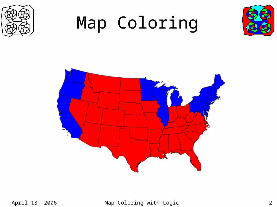
Map Coloring

April 13, 2006 Map Coloring with Logic 3
Map Coloring
• Color the nodes of the graph so that– no two adjacent nodes are the same color
April 13, 2006 Map Coloring with Logic 4
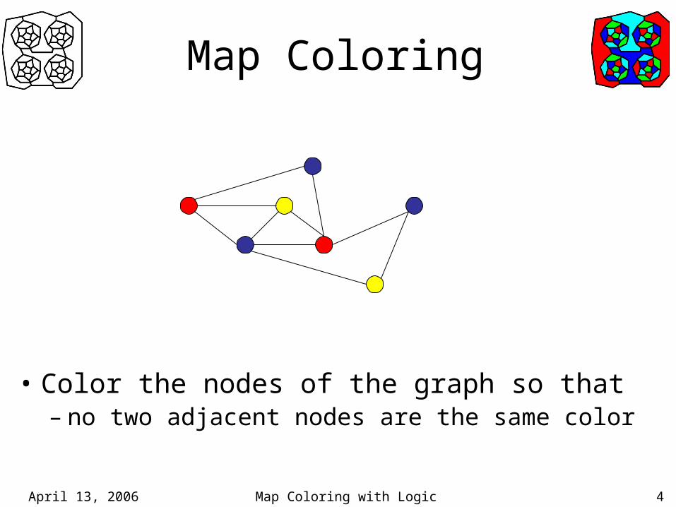
Map Coloring
• Color the nodes of the graph so that– no two adjacent nodes are the same color

April 13, 2006 Map Coloring with Logic 5
Student Formulation
Premises:color(X,C) => region(X)color(X,C) => hue(C)adjacent(X1,X2) ^ color(X1,C) => -color(X2,C)region(X) => Y.color(X,Y)
<ground atoms for adjacent, region, hue>
Query:TUVXYZ | color(r1,T) ^ color(r2,U) ^ color(r3,V) ^ …
- This is not the formulation used in the CSP/LP literature.- LP engines today do not understand this formulation.
r3 r6
r4 r2 r5
r1

April 13, 2006 Map Coloring with Logic 6
Logic Programming Formulation
• Axiomsnext(red,blue)next(red,green)next(red,yellow)next(blue,red)next(blue,green)…
• QueryR1 R2 R3 R4 R5 R6 | next(R1,R2) ^ next(R1,R3) ^ next(R1,R5) ^
next(R1,R6) ^ next(R2,R3) ^ next(R2,R4) ^ next(R2,R5) ^ next(R2,R6) ^ next(R3,R4) ^ next(R3,R6) ^ next(R5,R6)
This is the typical formulation used in the literature.This form (deductive) is required by LP.
r3 r6
r4 r2 r5
r1

April 13, 2006 Map Coloring with Logic 7
Map Coloring with Logic
• Two formulations1. The one students produce in CS157 every year
2. The one used in the literature [McCarthy82]
• (1) is more natural (and non-deductive)
(2) is more efficient (and deductive)
• Question for the day:– How do we translate (1) into (2)?

April 13, 2006 Map Coloring with Logic 8
Agenda
1. Consistency to Deduction: Reformulate non-deductive problem into deductive problem (a form of closing a theory)
2. Database Reformulation: turn output of (1) into the Logic Programming formulation.
3. Bilevel Reasoning: speeding up (1)

April 13, 2006 Map Coloring with Logic 9
Running Example
• Example: a very simple graph and two colors– 3 nodes, 2 edges– red and blue
Solutions:Problem:

April 13, 2006 Map Coloring with Logic 10
Constraint Satisfaction
• Definition (Constraint Satisfaction Problem):Input:
<V, DV, CV>
V: set of variables v1,v2,…
DV: domain for each variable -- dom(vi)
CV: constraints on values of variables
Output: Assignment of values to variables so that
1. val(vi) in dom(vi)2. all the constraints are satisfied
April 13, 2006 Map Coloring with Logic 11
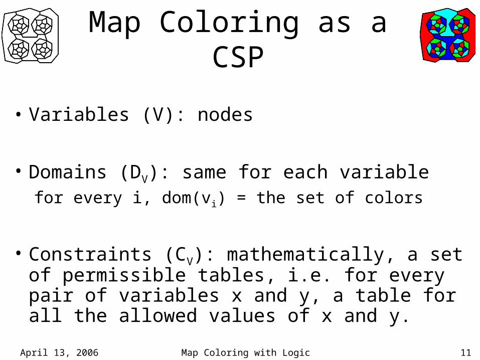
Map Coloring as a CSP
• Variables (V): nodes
• Domains (DV): same for each variablefor every i, dom(vi) = the set of colors
• Constraints (CV): mathematically, a set of permissible tables, i.e. for every pair of variables x and y, a table for all the allowed values of x and y.

April 13, 2006 Map Coloring with Logic 12
Example
V: {R1, R2, R3}
DV: dom(R1) = {r, b} dom(R2) = {r, b} dom(R3) = {r, b}
R1 R2
r b
b r
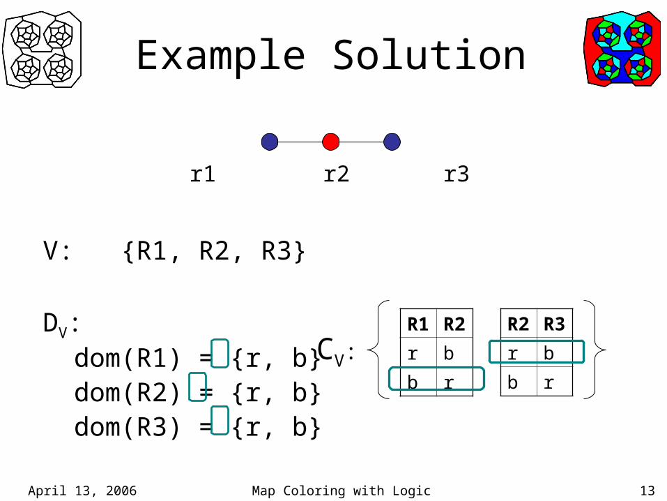
CV:
r1 r2 r3
R2 R3
r b
b r
April 13, 2006 Map Coloring with Logic 13
Example Solution
V: {R1, R2, R3}
DV: dom(R1) = {r, b} dom(R2) = {r, b} dom(R3) = {r, b}
R1 R2
r b
b r
CV:
r1 r2 r3
R2 R3
r b
b r
April 13, 2006 Map Coloring with Logic 14
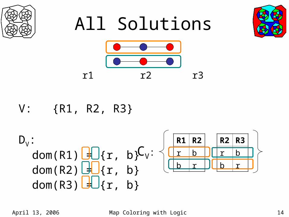
All Solutions
V: {R1, R2, R3}
DV: dom(R1) = {r, b} dom(R2) = {r, b} dom(R3) = {r, b}
R1 R2
r b
b r
CV:
r1 r2 r3
R2 R3
r b
b r

April 13, 2006 Map Coloring with Logic 15
All Solutions as a DB Query
• The set of all solutions can also be computed using the natural join operator.
r1 r2 r3
R1 R2
r b
b r
R2 R3
r b
b r=
R1 R2 R3
r b r
b r b

April 13, 2006 Map Coloring with Logic 16
Constraint Representations
• Representing constraints as permissible tables can be expensive and cumbersome.
• Often, constraints are more naturally and economically represented as logical sentences.

April 13, 2006 Map Coloring with Logic 17
Student Formulation
Premises:color(X,C) => region(X)color(X,C) => hue(C)adjacent(X1,X2) ^ color(X1,C) => -color(X2,C)region(X) => Y.color(X,Y)adjacent(r1,r2) ^ adjacent(r2,r3) ^ hue(r) ^ hue(b)region(r1) ^ region(r2) ^ region(r3)
Entailment Query:XYZ | color(r1,X) ^ color(r2,Y) ^ color(r3,Z)
Models:
r1 r2 r3

April 13, 2006 Map Coloring with Logic 18
Student Formulation
Premises:color(X,C) => region(X)color(X,C) => hue(C)adjacent(X1,X2) ^ color(X1,C) => -color(X2,C)region(X) => Y.color(X,Y)adjacent(r1,r2) ^ adjacent(r2,r3) ^ hue(r) ^ hue(b)region(r1) ^ region(r2) ^ region(r3)
Build a model:XYZ | color(r1,X) ^ color(r2,Y) ^ color(r3,Z)
Models:
r1 r2 r3

April 13, 2006 Map Coloring with Logic 19
Logic Programming Formulation
• Is different than the student formulation
• [McCarthy82] borrowed from Pereira and Porto [1980]– McCarthy started with their formulation and showed various
reformulations that improved efficiency.
– Served as an exploration of Kowalski’s doctrine:Algorithm = Logic + Control
• Originally used to illustrate issues in Constraint Satisfaction/Logic Programming

April 13, 2006 Map Coloring with Logic 20
LP Formulation
• Axioms
next(r,b)next(b,r)
• Entailment queryR1 R2 R3 | next(R1,R2) ^ next(R2,R3)
r1 r2 r3
Deductive

April 13, 2006 Map Coloring with Logic 21
Problem Statement• Produce an algorithm that converts
Axioms:color(X,C) => region(X)color(X,C) => hue(C)adjacent(X1,X2) ^ color(X1,C) => -color(X2,C)region(X) => Y.color(X,Y)…
Build Model: XYZ | color(r1,X) ^ color(r2,Y) ^ color(r3,Z)
intoAxioms:
next(red,blue)next(blue,red)
Entailment Query: XYZ | next(X,Y) ^ next(Y,Z)

April 13, 2006 Map Coloring with Logic 22
Herbrand Logic
• Assume no function constants
• The axioms include a – DCA over all ground terms – UNA over all ground terms
• Assume these hold implicitly– Finite Herbrand Logic
April 13, 2006 Map Coloring with Logic 23
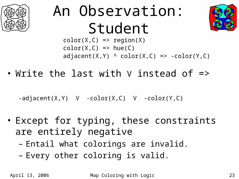
An Observation: Studentcolor(X,C) => region(X)color(X,C) => hue(C)adjacent(X,Y) ^ color(X,C) => -color(Y,C)
• Write the last with V instead of =>
-adjacent(X,Y) V -color(X,C) V -color(Y,C)
• Except for typing, these constraints are entirely negative– Entail what colorings are invalid.
– Every other coloring is valid.

April 13, 2006 Map Coloring with Logic 24
Student Coloringsadjacent(X,Y) ^ color(X,C) => -color(Y,C)
• Invalid answers (entailed) XYZ | -(color(r1,X) ^ color(r2,Y) ^ color(r3,Z))
• Remaining answers
…

April 13, 2006 Map Coloring with Logic 25
Idea
• To reformulate from Student to LP,1. Compute all invalid colorings (which are entailed).
2. Compute the complement of that set.
=
…

April 13, 2006 Map Coloring with Logic 26
Implementation
: the set of Student constraintsQuery: color(r1,X) ^ color(r2,Y) ^ color(r3,Z)
• Reify the notion of an invalid coloring.(*) invalid(X,Y,Z) <=>
-(color(r1,X) ^ color(r2,Y) ^ color(r3,Z))
• Ask for all the invalid colorings that are logically entailed.
XYZ | ^ (*) |= invalid(X,Y,Z)

April 13, 2006 Map Coloring with Logic 27
Implementation
XYZ | invalid(X,Y,Z)
• The following expression is logically entailed and represents the set of all invalid colorings:
X=r1 v X=r2 v X=r3 v Y=r1 v Y=r2 v Y=r3 v
Z=r1 v Z=r2 v Z=r3 v X=Y v Y=Z
X Y Z

April 13, 2006 Map Coloring with Logic 28
Implementation
• To compute an expression that represents the complement of that set, it turns out that all we need to do is negate that expression.
X≠r1 ^ X≠r2 ^ X≠r3 ^Y≠r1 ^ Y≠r2 ^ Y≠r3 ^Z≠r1 ^ Z≠r2 ^ Z≠r3 ^ X≠Y ^ Y≠Z
• The above (with unique names axioms) entails all the valid colorings.
X Y Z

April 13, 2006 Map Coloring with Logic 29
Progress: Both are deductive• Student after reformulation: all deductive answers to
XYZ | X≠r1 ^ X≠r2 ^ X≠r3 ^ Y≠r1 ^ Y≠r2 ^ Y≠r3 ^ Z≠r1 ^ Z≠r2 ^ Z≠r3 ^ X≠Z ^ Y≠Z
UNA[r,b,r1,r2,r3]
• LP formulation: all deductive answers toXYZ | next(X,Y) ^ next(Y,Z)next(r,b)next(b,r)
X Y Z
April 13, 2006 Map Coloring with Logic 30
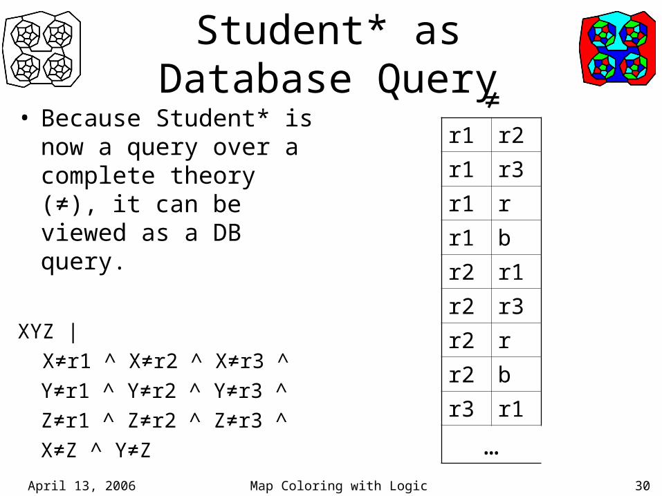
Student* as Database Query
• Because Student* is now a query over a complete theory (≠), it can be viewed as a DB query.
XYZ | X≠r1 ^ X≠r2 ^ X≠r3 ^
Y≠r1 ^ Y≠r2 ^ Y≠r3 ^Z≠r1 ^ Z≠r2 ^ Z≠r3 ^X≠Z ^ Y≠Z
r1 r2
r1 r3
r1 r
r1 b
r2 r1
r2 r3
r2 r
r2 b
r3 r1
…
≠

April 13, 2006 Map Coloring with Logic 31
Database Reformulation
• Given one database query, find an equivalent query that is more efficient.– Includes performing transformations on the data itself, with a
space limit.
• Theorem [Chirkova]: There are infinitely many distinct transformations.
• Theorem [Chirkova]: There is an algorithm that given the query constructs a finite space of queries that is guaranteed to include the optimal one.
April 13, 2006 Map Coloring with Logic 32
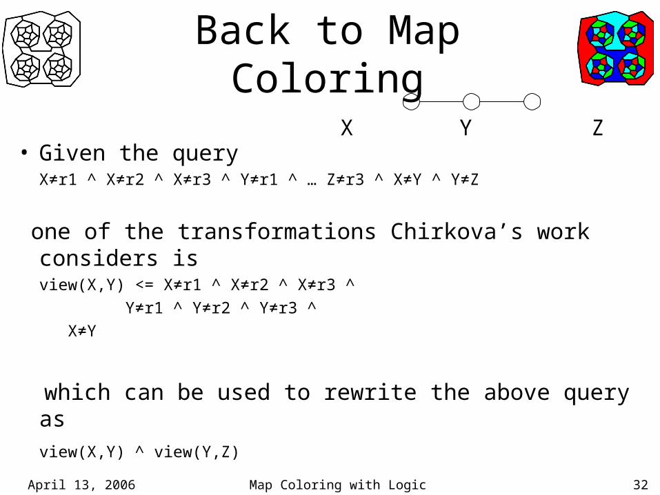
Back to Map Coloring
• Given the queryX≠r1 ^ X≠r2 ^ X≠r3 ^ Y≠r1 ^ … Z≠r3 ^ X≠Y ^ Y≠Z
one of the transformations Chirkova’s work considers isview(X,Y) <= X≠r1 ^ X≠r2 ^ X≠r3 ^ Y≠r1 ^ Y≠r2 ^ Y≠r3 ^
X≠Y
which can be used to rewrite the above query asview(X,Y) ^ view(Y,Z)
X Y Z

April 13, 2006 Map Coloring with Logic 33
Comparison
• Student**XYZ | view(X,Y) ^ view(Y,Z)view(r,b)view(b,r)
• Logic ProgrammingXYZ | next(X,Y) ^ next(Y,Z)next(r,b)next(b,r)
X Y Z

April 13, 2006 Map Coloring with Logic 34
Overview• Starting with the Student formulation,
XYZ | color(r1,X) ^ color(r2,Y) ^ color(r3,Z) color(X,C) => region(X) color(X,C) => hue(C) adjacent(X1,X2) ^ color(X1,C) => -color(X2,C)
use logical entailment to find an expression for all the invalid colorings and negate it. XYZ | X≠r1 ^ X≠r2 ^ X≠r3 ^ … ^ X≠Y ^ Y≠Z
• Then apply Chirkova’s work to produce the LP formulation, or one that is at least as good as LP. XYZ | view(X,Y) ^ view(Y,Z)
April 13, 2006 Map Coloring with Logic 35
Another Example
• N-Queens: place N queens on an NxN chessboard s.t.– No queen can be attacked by another queen.
That is– No two queens share the same row– No two queens share the same column– No two queens share the same diagonal

April 13, 2006 Map Coloring with Logic 36
8 Queens Solution

April 13, 2006 Map Coloring with Logic 37
N-Queens Constraints
• All queens in different rowsX≠Y ^ row(X,R) => -row(Y,R)
• All queens in different columnsX≠Y ^ col(X,C) => -col(Y,C)
• All queens in different diagonalsX≠Y ^ diag(X,D1,D2)
=> -diag(Y,D1,D2)
April 13, 2006 Map Coloring with Logic 38
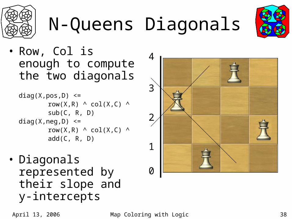
N-Queens Diagonals• Row, Col is enough to
compute the two diagonals
diag(X,pos,D) <= row(X,R) ^ col(X,C) ^ sub(C, R, D)
diag(X,neg,D) <= row(X,R) ^ col(X,C) ^ add(C, R, D)
• Diagonals represented by their slope and y-intercepts
0
1
2
3
4

April 13, 2006 Map Coloring with Logic 39
4 Queens Query
• Satisfiability Query:
(X1 Y1 X2 Y2 X3 Y3 X4 Y4) |
row(q1,X1) ^ col(q1,Y1) ^row(q2,X2) ^ col(q2,Y2) ^row(q3,X3) ^ col(q3,Y3) ^row(q4,X4) ^ col(q4,Y4)

April 13, 2006 Map Coloring with Logic 40
Efficiency in N-Queens
• The expression that represents all invalid positions can become quite large and might take a long time to compute because of the add and sub facts.– About 150 conjuncts
• Idea: produce an expression in terms of add and sub, as well as =.
April 13, 2006 Map Coloring with Logic 41
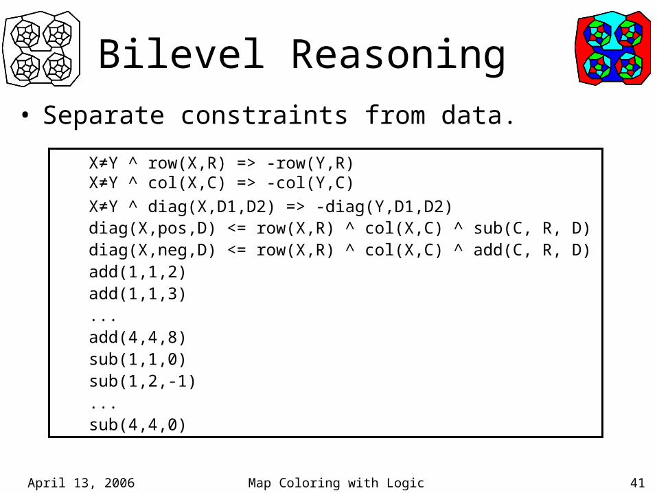
Bilevel Reasoning • Separate constraints from data.
X≠Y ^ row(X,R) => -row(Y,R)X≠Y ^ col(X,C) => -col(Y,C)X≠Y ^ diag(X,D1,D2) => -diag(Y,D1,D2)diag(X,pos,D) <= row(X,R) ^ col(X,C) ^ sub(C, R, D)diag(X,neg,D) <= row(X,R) ^ col(X,C) ^ add(C, R, D)add(1,1,2)add(1,1,3)...add(4,4,8)sub(1,1,0)sub(1,2,-1)...sub(4,4,0)

April 13, 2006 Map Coloring with Logic 42
Bilevel Reasoning • Separate constraints from data.
X≠Y ^ row(X,R) => -row(Y,R)X≠Y ^ col(X,C) => -col(Y,C)X≠Y ^ diag(X,D1,D2) => -diag(Y,D1,D2)diag(X,pos,D) <= row(X,R) ^ col(X,C) ^ sub(C, R, D)diag(X,neg,D) <= row(X,R) ^ col(X,C) ^ add(C, R, D)add(1,1,2)add(1,1,3)...add(4,4,8)sub(1,1,0)sub(1,2,-1)...sub(4,4,0)

April 13, 2006 Map Coloring with Logic 43
X≠Y ^ row(X,R) => -row(Y,R)X≠Y ^ col(X,C) => -col(Y,C)X≠Y ^ diag(X,D1,D2) => -diag(Y,D1,D2)diag(X,pos,D) <= row(X,R) ^ col(X,C) ^ sub(C, R, D)diag(X,neg,D) <= row(X,R) ^ col(X,C) ^ add(C, R, D)
Bilevel Reasoning • Separate constraints from data.
add(1,1,2)add(1,1,3)...add(4,4,8)sub(1,1,0)sub(1,2,-1)...sub(4,4,0)
April 13, 2006 Map Coloring with Logic 44
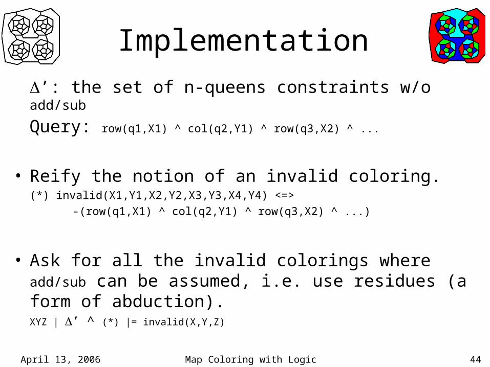
Implementation
’: the set of n-queens constraints w/o add/sub
Query: row(q1,X1) ^ col(q2,Y1) ^ row(q3,X2) ^ ...
• Reify the notion of an invalid coloring.(*) invalid(X1,Y1,X2,Y2,X3,Y3,X4,Y4) <=>
-(row(q1,X1) ^ col(q2,Y1) ^ row(q3,X2) ^ ...)
• Ask for all the invalid colorings where add/sub can be assumed, i.e. use residues (a form of abduction).XYZ | ’ ^ (*) |= invalid(X,Y,Z)

April 13, 2006 Map Coloring with Logic 45
4-Queens Partial Reformulation
goal(X1,Y1,X2,Y2,X3,Y3,X4,Y4) <=
X1 ≠ X2
Y1 ≠ Y2(-sub(Y2,X2,Z) v -sub(Y1,X1,Z))(-add(Y2,X2,Z)) v -add(Y1,X1,Z))
X1 ≠ X3
Y1 ≠ Y3
X2 ≠ X3
Y2 ≠ Y3(-sub(Y3,X3,Z) v -sub(Y1,X1,Z))(-sub(Y3,X3,Z) v -sub(Y2,X2,Z))(-add(Y3,X3,Z) v -add(Y1,X1,Z))(-add(Y3,X3,Z) v -add(Y2,X2,Z))...

April 13, 2006 Map Coloring with Logic 46
Consistency to Deduction• Computing the sentences that are consistent with the
premises and making them deductive consequences. • Definition (query consistency to deduction):
qC2D[, (xbar)] = {tbar | (tbar) is satisfiable}
• In map coloring, = the set of map coloring axioms(xbar) = color(r1,X) ^ color(r2,Y) ^ color(r3,Z) qC2D = {<r,b,r>, <b,r,b>}

April 13, 2006 Map Coloring with Logic 47
Descriptions• Definition (Description): e(xbar) is a description for the set of
n-tuples S, where |xbar| = n if and only if|= e(tbar) if tbar S|= -e(tbar) if tbar S
• Example: X=Y V Y=Z describes {rrr,rrb,brr,bbr,rbb,bbb} in FHL
|=H r=r V r=r |=H r=r V r=b |=H b=r V r=r
|=H b=b V b=r |=H r=b V b=b |=H b=b V b=b
and|=H -(r=b V b=r)
|=H -(b=r V r=b)

April 13, 2006 Map Coloring with Logic 48
Algorithm
• Input : a finite set of FHL sentences
(xbar): a query in the vocabulary of Delta
1. Using algorithm Alg, compute an expression e(xbar) in terms of equality such that for any model M in R,
|=M e(tbar) if and only if |= -(tbar)
2. Output -e(xbar)

April 13, 2006 Map Coloring with Logic 49
Theorems
• Theorem (Soundness and Completeness): Let Alg(, (xbar)) = -e(xbar).
|=M -e(tbar) if and only if (tbar) qC2D[, (xbar)]Proof: Nontrivial
• Theorem (Decidability): qC2D[, (xbar)] for FHL is decidable.Proof: Walk over Herbrand models and if |=M , collect all tbar
s.t. |=M (tbar)

April 13, 2006 Map Coloring with Logic 50
Relationship to CWA
• CWA[] includes -p(tbar) whenever |# p(tbar)
• CWA[] is inconsistent whenever – Delta entails some disjunction d1 v … v dn and
– Delta entails none of the di.
• Adding the map coloring answers to the Student formulation is inconsistent.
April 13, 2006 Map Coloring with Logic 51
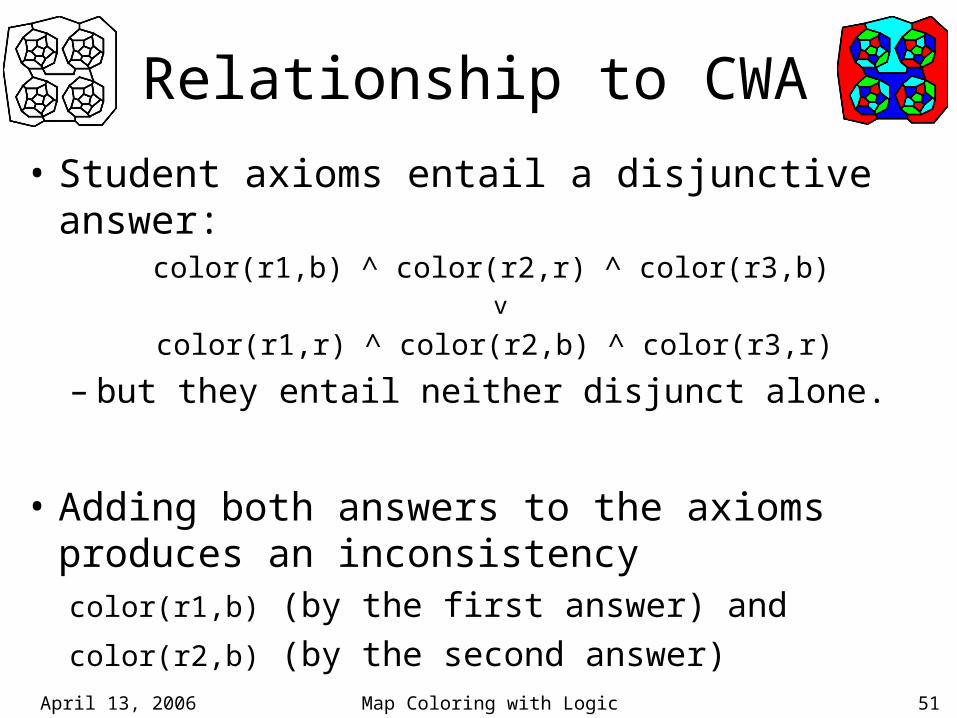
Relationship to CWA
• Student axioms entail a disjunctive answer:color(r1,b) ^ color(r2,r) ^ color(r3,b)
v
color(r1,r) ^ color(r2,b) ^ color(r3,r)
– but they entail neither disjunct alone.
• Adding both answers to the axioms produces an inconsistencycolor(r1,b) (by the first answer) and
color(r2,b) (by the second answer)

April 13, 2006 Map Coloring with Logic 52
Relationship to CWA
• CWA: for every ground p, add -p if p is not entailed.
• C2D: for every ground p, add p if -p is not entailed.

April 13, 2006 Map Coloring with Logic 53
Map Coloring with Logic[McCarthy82] McCarthy.
Coloring Maps and the Kowalski Doctrine. Stanford Tech Report 1982.
[Pereira80] Pereira and Porto. Selective Backtracking for Logic Programs. CADE 1980.
[Chirkova2002] Chirkova. Automated Database Restructuring. Stanford thesis 2002.

April 13, 2006 Map Coloring with Logic 54
Scrap starts here

April 13, 2006 Map Coloring with Logic 55
Bilevel Reasoning • Separate constraints from data.
color(X,C) => region(X)color(X,C) => hue(C)adjacent(X1,X2) ^ color(X1,C) => -color(X2,C)adjacent(r1,r2)adjacent(r2,r3)hue(r)hue(b)region(r1)region(r2)region(r3)

April 13, 2006 Map Coloring with Logic 56
Bilevel Reasoning • Separate constraints from data.
color(X,C) => region(X)color(X,C) => hue(C)adjacent(X1,X2) ^ color(X1,C) => -color(X2,C)adjacent(r1,r2)adjacent(r2,r3)hue(r)hue(b)region(r1)region(r2)region(r3)

April 13, 2006 Map Coloring with Logic 57
Bilevel Reasoning • Separate constraints from data.
color(X,C) => region(X)color(X,C) => hue(C)adjacent(X1,X2) ^ color(X1,C) => -color(X2,C)
adjacent(r1,r2)adjacent(r2,r3)hue(r)hue(b)region(r1)region(r2)region(r3)

April 13, 2006 Map Coloring with Logic 58
Bilevel Map coloring
• It turns out that separating hue off from the rest of the axioms is an interesting case.
color(X,C) => region(X)color(X,C) => hue(C)adjacent(X1,X2) ^ color(X1,C) => -color(X2,C)adjacent(r1,r2)adjacent(r2,r3)region(r1)region(r2)region(r3)
hue(r)hue(b)

April 13, 2006 Map Coloring with Logic 59
Partial Reformulation• The algorithm presented earlier started with axioms
talking about hues, regions, adjacency, and coloradjacent(X,Y) ^ color(X,C) => -color(Y,C)
to produceXYZ | X≠r1 ^ X≠r2 ^ X≠r3 ^
Y≠r1 ^ Y≠r2 ^ Y≠r3 ^Z≠r1 ^ Z≠r2 ^ Z≠r3 ^X≠Z ^ Y≠Z
but if we separate hue we should get the following resultXYZ | hue(X) ^ hue(Y) ^ hue(Z) ^ X≠Y ^ Y≠Z
X Y Z

April 13, 2006 Map Coloring with Logic 60
Implementation
• Epilog (the Logic Group’s theorem prover) produces an expression that represents the set of all invalid colorings, in terms of hue:
XYZ | invalid(X,Y,Z), wrt hue=> -hue(X) v -hue(Y) v -hue(Z) v X=Y v Y=Z
• Negating (just as before) gives ushue(X) ^ hue(Y) ^ hue(Z) ^ X≠Y ^ Y≠Z
X Y Z

April 13, 2006 Map Coloring with Logic 61
Database Reformulation
• Given: a schema R and a set of queries Q={Q1,…,Qn}– Compute a set of views on R that minimize the cost of
evaluating all the Qi.
(Each relation in R is assigned a size.)
• Rada Chirkova [Chirkova2002]: conjunctive queries.– Decidable.
– Triply exponential upper bound (in Q).
– Exponential lower bound (in Q).
April 13, 2006 Map Coloring with Logic 62
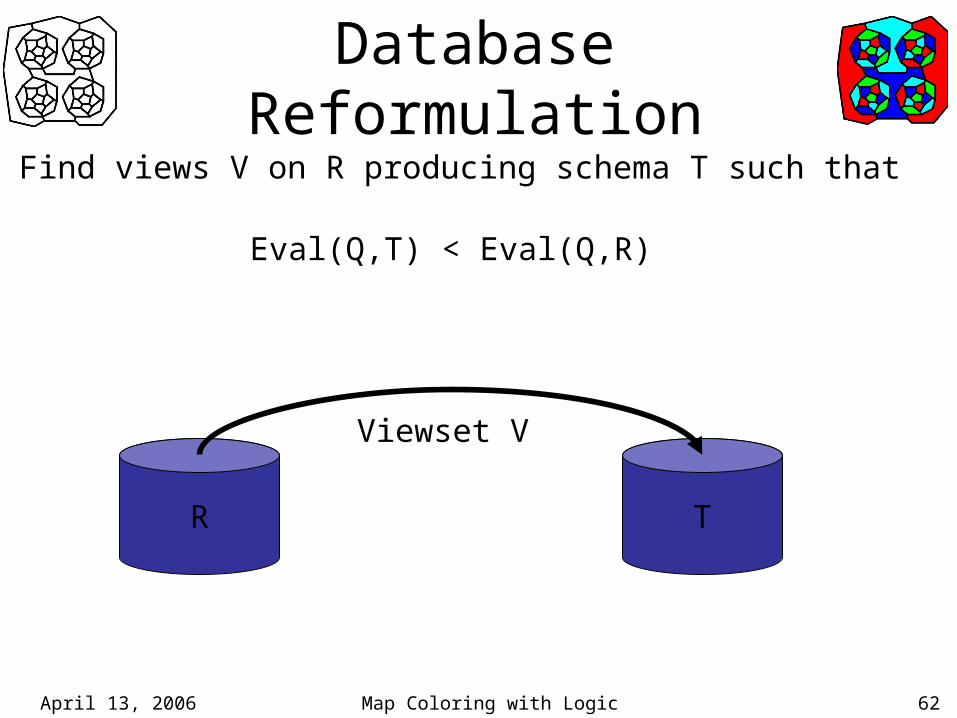
Database Reformulation
R T
Eval(Q,T) < Eval(Q,R)
Find views V on R producing schema T such that
Viewset V

April 13, 2006 Map Coloring with Logic 63
Example
• Schema: parent(x,y)
• Query: XY | samefamily(X,Y)
samefamily(X,Y) <= anc(X,Z) ^ anc(Y,Z)
anc(X,Y) <= parent(X,Y)anc(X,Y) <= anc(X,Z) ^ anc(Z,Y)
• Can be evaluated more efficiently as: samefamily(X,Y) <=
foundingfather(X,F) ^ foundingfather(Y,F)

April 13, 2006 Map Coloring with Logic 64
Map Coloring in Math• 1852: Guthrie makes Four Colour Conjecture:
Any planar graph can be colored using only four colors.
• Definition(Planar graph): Graph that can be drawn on the plane without edges crossing.
• Incorrect proofs given by Kempe (1879) and Tait (1880). Kempe’s was accepted for over a decade.
• 1977: Appel and Haken wrote a program to exhaustively check a large number of cases. They (debatably) proved the conjecture.
April 13, 2006 Map Coloring with Logic 65
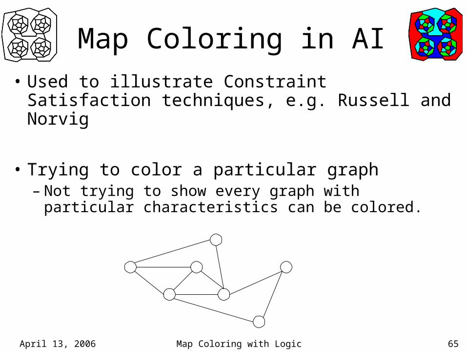
Map Coloring in AI
• Used to illustrate Constraint Satisfaction techniques, e.g. Russell and Norvig
• Trying to color a particular graph– Not trying to show every graph with particular
characteristics can be colored.

April 13, 2006 Map Coloring with Logic 66
Student Formulation (2)
Premises:color(X,C) => region(X)color(X,C) => hue(C)adjacent(X1,X2) ^ color(X1,C) => -color(X2,C)
adjacent(r1,r2) ^ adjacent(r2,r3) ^ hue(r) ^ hue(b)region(r1) ^ region(r2) ^ region(r3)
Build a model:
r1 r2 r3
…

April 13, 2006 Map Coloring with Logic 67
DB Reformulation Again• Given the query
hue(X) ^ hue(Y) ^ hue(Z) ^ X≠Y ^ Y≠Z
one of the views Rada’s work considers is
view(X,Y) <= hue(X) ^ hue(Y) ^ X≠Y
which can be used to rewrite the above query as
view(X,Y) ^ view(Y,Z)
X Y Z

April 13, 2006 Map Coloring with Logic 68
Back to Map coloring• In Student*, the schema consists of a single relation: ≠.
• The query XYZ | X≠r1 ^ X≠r2 ^ X≠r3 ^
Y≠r1 ^ Y≠r2 ^ Y≠r3 ^Z≠r1 ^ Z≠r2 ^ Z≠r3 ^X≠Z ^ Y≠Z
• Unfortunately, this query includes constants, which Rada’s work does not cover.– Notice that this query is defined in terms of -hue.
X Y Z

April 13, 2006 Map Coloring with Logic 69
Efficiency
• It is unsettling and inefficient to have the answer defined in terms of -hue when it is more natural to define it in terms of hue.
hue(X) ^hue(Y) ^hue(Z) ^X ≠ Y ^Y ≠ Z
– Independent of which colors are available
– No constants
X Y Z

April 13, 2006 Map Coloring with Logic 70
A Technical Note about Descriptions
• e(X,Y,Z) <=> X=Y V Y=Z describes S = {rrr,rrb,brr,bbr,rbb,bbb}
For every tuple tbar in S, |=H e(tbar)
For every tuple tbar not in S, |=H -e(tbar)
• In Herbrand logic, suppose we know that 1. |=H e(tbar) implies tbar in S2. e(xbar) is built on a single relation constant: =. Then e(xbar) is a description of S.
April 13, 2006 Map Coloring with Logic 71
Issues
• Need efficient algorithm for computing all solutions in FHL that terminates.– Would settle for termination on clausal form.
• OSHL[Zhu,Plaisted]
• Model Evolution[Baumgartner]
• Computing the complement via negation worked well for map coloring, but in general it may be expensive when converting to clausal form (CNF to DNF).

April 13, 2006 Map Coloring with Logic 72
An Observation about McCarthy
XYZ | next(X,Y) ^ next(Y,Z)
• The valid colorings are entailed

April 13, 2006 Map Coloring with Logic 73
Complexity Analysis
• CS157hue(X) ^ hue(Y) ^ hue(Z) ^ X≠Y ^ Y≠Z hue(red) red ≠ bluehue(blue) blue ≠ red
• McCarthynext(X,Y) ^ next(Y,Z)next(red,blue)next(blue,red)
• Compare on trees. C=# of colors, N=# of nodes

April 13, 2006 Map Coloring with Logic 74
Asymptotic Complexity Results for Trees
1. hue(X) ^ hue(Y) ^ hue(Z) ^ X≠Y ^ Y≠Z• O(CN)
2. hue(X) ^ hue(Y) ^ X≠Y ^ hue(Z) ^ Y≠Z• O(CN-1)
3. next(X,Y) ^ next(Y,Z)• O(CN-2)
4. Same as 3 but indexed on first argument of next.• O(CN-3)

April 13, 2006 Map Coloring with Logic 75
Back to FOL
• If we are using first-order deduction procedures to answer finite Herbrand entailment queries, need a DCA and UNA.
• [Reiter80] showed that for * queries, DCA is unnecessary.

April 13, 2006 Map Coloring with Logic 76
Looks can be deceiving
• Suppose there were object constants besides red and blue, e.g. paperclip
• New axioms:-r1(X) V -r2(X)-r3(X) V -r2(X)
r1(X) V r2(X) V r3(X) => hue(X)hue(red)hue(blue)
-hue(paperclip)

April 13, 2006 Map Coloring with Logic 77
Running the algorithm:
• After conversion:
goal(X,Y,Z) <=> X ≠ paperclip ^X ≠ Y ^Y ≠ paperclip ^Y ≠ Z ^Z ≠ paperclip
1. Linear in the size of -hue(x)2. Not the same as the McCarthy formulation

April 13, 2006 Map Coloring with Logic 78
Solving CSPs as DB queries
• Can every CSP be formulated as a DB query?– Map coloring can be formulated as a DB query.
• When is it beneficial to solve a CSP by translating it into a DB query?– Under some conditions, it is beneficial for map coloring.
• Can the transformation be automated?

April 13, 2006 Map Coloring with Logic 79
Language of Study
• Option 1 (Mathematics): Explore algorithms of the following sort.– Input: <V, DV, CV>, i.e. a set, a set of functions, and a set of
tables.
– Output: <D, (x1,…,xn)>, i.e. a database and a query over that database.
• Option 2 (Logic): Explore algorithms of the following sort.– Input: Description of a CSP in logic.
– Output: Description of the database and the query in logic.

April 13, 2006 Map Coloring with Logic 80
CS157 Orderings
1. hue(X) ^ hue(Y) ^ hue(Z) ^ X≠Y ^ Y≠Z• Walk hue space and check each point.
2. X≠Y ^ Y≠Z ^ hue(X) ^ hue(Y) ^ hue(Z)• Walk ≠ space and check each point.
3. hue(X) ^ hue(Y) ^ X≠Y ^ hue(Z) ^ Y≠Z• Walk hue space, pruning as we go.
4. X≠Y ^ hue(X) ^ hue(Y) ^ Y≠Z ^ hue(Z)• Walk ≠ space, pruning as we go.

April 13, 2006 Map Coloring with Logic 81
On the Complexity of Query Evaluation
• Complexity depends heavily on indexing.
• Four options1. Relational: index only on the relation of facts
2. Relational + attach : eval ≠ in code
3. Arguments: index on reln and each argument position
4. Arguments + attach

April 13, 2006 Map Coloring with Logic 82
Some Connections
• Some connections to other work
– CWA– Applicability to Datalog queries

April 13, 2006 Map Coloring with Logic 83
Closed World Assumption
• qC2D and CWA are closely related
• In fact, a generalization of qC2D and CWA are nearly equivalent. – If we could compute CWA efficiently, that might help
us compute qC2D efficiently.
April 13, 2006 Map Coloring with Logic 84
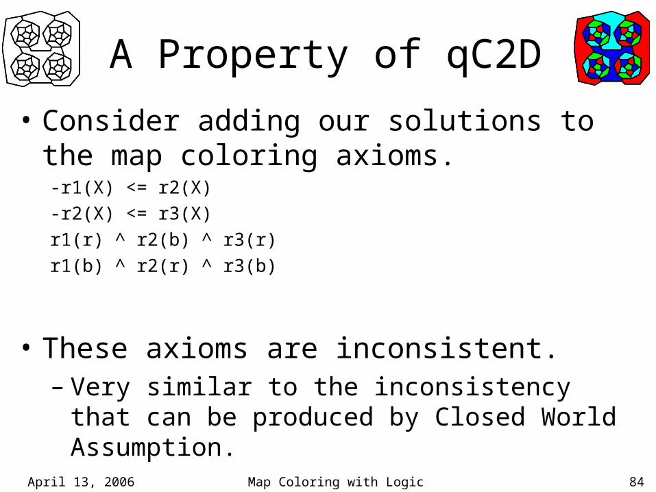
A Property of qC2D
• Consider adding our solutions to the map coloring axioms.-r1(X) <= r2(X)-r2(X) <= r3(X)r1(r) ^ r2(b) ^ r3(r)r1(b) ^ r2(r) ^ r3(b)
• These axioms are inconsistent. – Very similar to the inconsistency that can be produced
by Closed World Assumption.

April 13, 2006 Map Coloring with Logic 85
Closed World
• Definition (Set-based CWA): Let P={p1,…,pn} be a set of closed sentences.
sCWA[, P] = {-pi | |# pi}
• Example: = {q(a), q(b)}
P = {q(a), q(c)}
sCWA[, P] = {-q(c)}
• sCWA generalizes the standard definition for CWA

April 13, 2006 Map Coloring with Logic 86
sC2D
• For comparison to sCWA, we define sC2D.
• Definition (sC2D): Let P={p1,…,pn} be a set of sentences.
sC2D[, P] = {pi | pi is satisfiable}
• Theorem: Let {p1,…,pn} be a set of ground atoms.
sCWA[, {p1,…,pn}] = sC2D[, {-p1,…,-pn}]

April 13, 2006 Map Coloring with Logic 87
An Application• Suppose we have some set of Datalog sentences and a
negative query.:- not r(X), not s(Y), not p(Z)
• One approach:goal(X,Y,Z) :- univ(X), univ(Y), univ(Z),
not r(X), not s(Y), not p(Z)
• Cost: |univ|3
• If we had an explicit definition for the negative theory, the cost might be substantially less.

April 13, 2006 Map Coloring with Logic 88
An Application (2)
Data:p(a,b) p(b,a) p(c,a) p(d,a)p(a,c) p(b,c) p(c,b) p(d,b)p(a,d) p(b,d) p(c,d) p(d,c)
Query: univ(X), univ(Y), not p(X,Y)Cost: |univ|2
Query: univ(X), not p(X,X)Cost: |univ|

April 13, 2006 Map Coloring with Logic 89
Computing the Complement
In Map Coloring• Expression for invalid
colorsX=Y V Y=Z
• Negation of that expressionX#Y ^ Y#Z
• Final reformulationgoal(X,Y,Z) <= X#Y ^ Y#Z
More generally• Expression for entailed
negations of query(xbar)
• Negation of that expression-(xbar)
• Final reformulationgoal(xbar) <= -(xbar)

April 13, 2006 Map Coloring with Logic 90
Questions
• Every relation in a theory with a DCA can be defined entirely in terms of equality.
• Question: When can we use fullfinds to compute that definition? (logically justified)
• Question: When should we use fullfinds to compute that definition? (computability/complexity justified)
April 13, 2006 Map Coloring with Logic 91
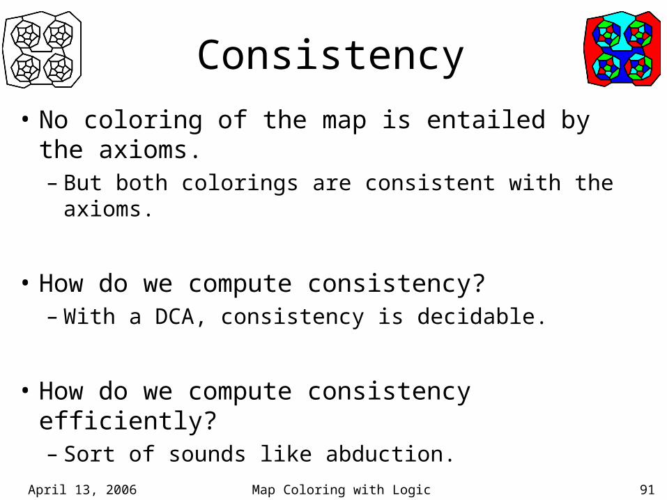
Consistency
• No coloring of the map is entailed by the axioms.– But both colorings are consistent with the axioms.
• How do we compute consistency?– With a DCA, consistency is decidable.
• How do we compute consistency efficiently?– Sort of sounds like abduction.

April 13, 2006 Map Coloring with Logic 92
Abduction
• Definition (Abduction): explains |= in the language L if and only if
1. |= 2. is consistent
3. is in L
• Let be the map coloring axioms
– r1(r) ^ r2(b) ^ r3(r) explains |= XYZ. r1(X) ^ r2(Y) ^ r3(Z)

April 13, 2006 Map Coloring with Logic 93
Attempt #3
• Residue attempts to compute abductive consequences
-r1(X) <= r2(X)-r2(X) <= r3(X)goal(X,Y,Z) <= r1(X) ^ r2(Y) ^ r3(Z)
? (fullresidue '(goal ?x ?y ?z) 'mapc)Call: (GOAL ?X ?Y ?Z) | Call: (R1 ?X) | Fail: (R1 ?X)Fail: (GOAL ?X ?Y ?Z)
• Equality does not help.
April 13, 2006 Map Coloring with Logic 94
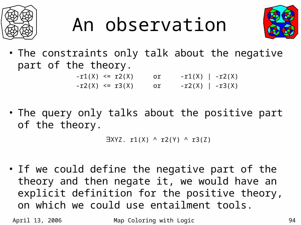
An observation
• The constraints only talk about the negative part of the theory.
-r1(X) <= r2(X) or -r1(X) | -r2(X)-r2(X) <= r3(X) or -r2(X) | -r3(X)
• The query only talks about the positive part of the theory. XYZ. r1(X) ^ r2(Y) ^ r3(Z)
• If we could define the negative part of the theory and then negate it, we would have an explicit definition for the positive theory, on which we could use entailment tools.

April 13, 2006 Map Coloring with Logic 95
Reformulation and Completion
1. Temporarily add the goal to the original axioms.-r1(X) <= r2(X)-r2(X) <= r3(X)goal(X,Y,Z) <=> r1(X) ^ r2(Y) ^ r3(Z)
2. Capture the negative query in terms of equality.-goal(X,Y,Z) <= X=Y | Y=Z
3. Apply predicate completion-goal(X,Y,Z) <=> X=Y | Y=Z goal(X,Y,Z) <=> X#Y ^ Y#Z
4. Assuming UNAxioms, ask for goal(X,Y,Z).
April 13, 2006 Map Coloring with Logic 96
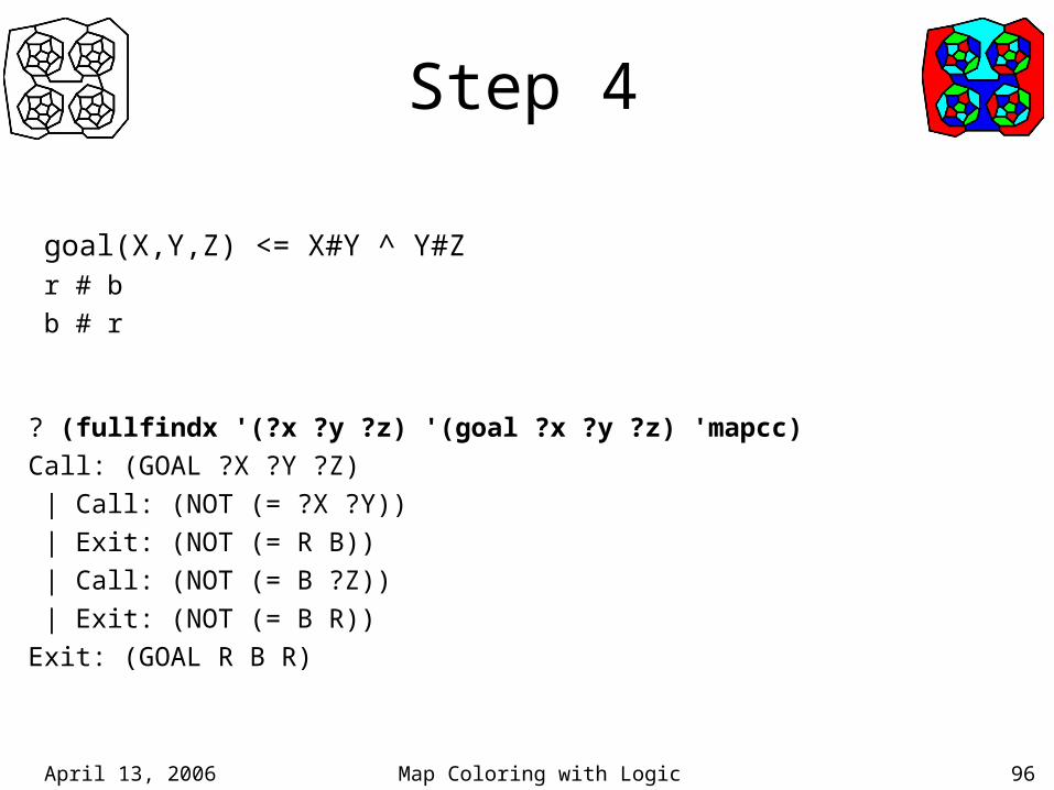
Step 4
goal(X,Y,Z) <= X#Y ^ Y#Z r # b b # r
? (fullfindx '(?x ?y ?z) '(goal ?x ?y ?z) 'mapcc)Call: (GOAL ?X ?Y ?Z) | Call: (NOT (= ?X ?Y)) | Exit: (NOT (= R B)) | Call: (NOT (= B ?Z)) | Exit: (NOT (= B R))Exit: (GOAL R B R)

April 13, 2006 Map Coloring with Logic 97
Step 2 -r1(X) <= r2(X)
-r2(X) <= r3(X)
goal(X,Y,Z) <= r1(X) ^ r2(Y) ^ r3(Z)-goal(X,Y,Z) <= -r1(X)-goal(X,Y,Z) <= -r2(X)-goal(X,Y,Z) <= -r3(X)
r1(X) <= goal(X,Y,Z)r2(Y) <= goal(X,Y,Z)r3(Z) <= goal(X,Y,Z)
? (fullfinds '(?x ?y ?z) '(not (goal ?x ?y ?z)) 'mapc)((?u ?u ?w) (?u ?w ?w))

April 13, 2006 Map Coloring with Logic 98
Back to the CSP Version
V: {v1,v2,v3}
DV: {{r, b},{r, b},{r, b}}
CV:
v1 v2
r b
b r
v2 v3
r b
b r
goal(X,Y,Z) <= X#Y ^ Y#Zr # bb # r

April 13, 2006 Map Coloring with Logic 99
CS157 Formulation (3)
Premises: Models:X=red | X=blue-r1(X) <= r2(X)-r2(X) <= r3(X)
X.r1(X)
X.r2(X)
X.r3(X)
Satisfaction Query: XYZ | r1(X) ^ r2(Y) ^ r3(Z)
– All resolution-style t.p. return something like
In general, adding these sentencesmay cause inconsistency.
k1, k2, k3

April 13, 2006 Map Coloring with Logic 100
Example
V: {v1,…,v7}
DV:
dom(v1) = {r,y,b}
…
dom(v7) = {r,y,b}
v1 v2
r y
r b
y b
y r
b y
b r
1
24
5
3
6
7
v6 v7
r y
r b
y b
y r
b y
b r
CV: ,…,

April 13, 2006 Map Coloring with Logic 101
Example
V: {v1,…,v7}
DV:
dom(v1) = {r,y,b}
…
dom(v7) = {r,y,b}
v1 v2
r y
r b
y b
y r
b y
b r
v6 v7
r y
r b
y b
y r
b y
b r
CV: ,…,
1
24
5
3
6
7
April 13, 2006 Map Coloring with Logic 102
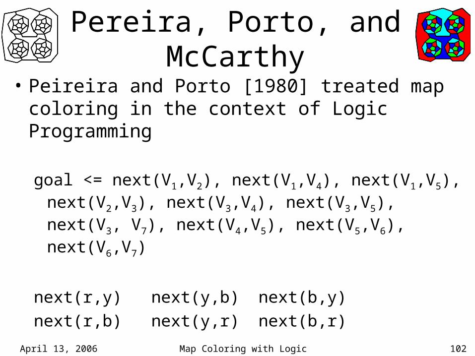
Pereira, Porto, and McCarthy
• Peireira and Porto [1980] treated map coloring in the context of Logic Programming
goal <= next(V1,V2), next(V1,V4), next(V1,V5), next(V2,V3), next(V3,V4), next(V3,V5), next(V3, V7), next(V4,V5), next(V5,V6), next(V6,V7)
next(r,y) next(y,b) next(b,y)
next(r,b) next(y,r) next(b,r)

April 13, 2006 Map Coloring with Logic 103
Why does this work?
• Reformulation (Step 2) rewrites the negation of the query in terms of just equality. – For larger map colorings, there will be O(n2) answers
to -goal(X,Y,Z), where n = # of regions.
• At an abstract level, it enumerates all the cases where -goal(X,Y,Z) is directly entailed
• Everything else is thrown into goal.