Approximating The Permanent

Amit Kagan

Seminar in Complexity04/06/2001

Topics

• Description of the Markov chain

• Analysis of its mixing time

Definitions

• Let G = (V1, V2, E) be a bipartite graph on n+n vertices.

• Let denote the set of perfect matchings in G.

• Let (y, z) denote the set of near-perfect matchings with holes only at y and z.

• ),(, zyzy

|(u,v)|/|| Exponentially Large

It has only one perfect matching...

u v

Observe the following bipartite graph:

|(u,v)|/|| Exponentially Large

But two near-perfect matchings with holes at u and v.

u v

|(u,v)|/|| Exponentially Large

• Concatenating another hexagon,– adds a constant number of vertices,

– but doubles the number of near-perfect matchings,

– while the number of perfect matchings remains 1.

. . .

Thus we can force the ratio |(u,v)|/|| to be exponentially large.

The Breakthrough

• Jerrum, Sinclair, and Vigoda [2000] introduced an additional weight factor.

• Any hole pattern (including that with no holes) is equally likely in the stationary distribution π.

• π will assign Ω(1/n2) weight to perfect matchings.

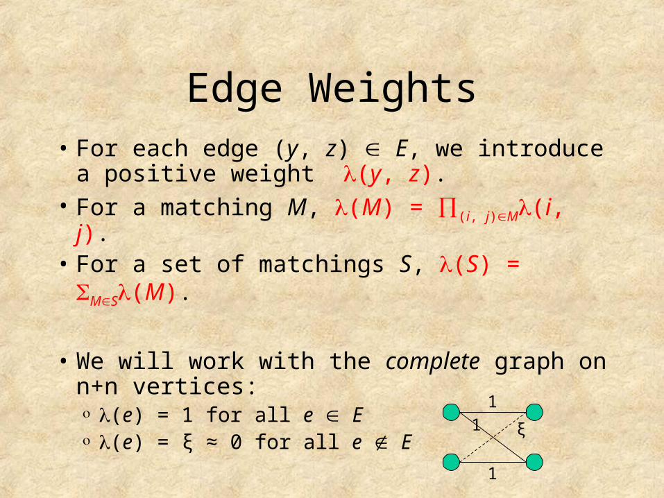
Edge Weights

• For each edge (y, z) E, we introduce a positive weight (y, z).

• For a matching M, (M) = (i, j)M(i, j).• For a set of matchings S, (S) = MS(M).

• We will work with the complete graph on n+n vertices: (e) = 1 for all e E (e) = ξ ≈ 0 for all e E

1

1

1 ξ

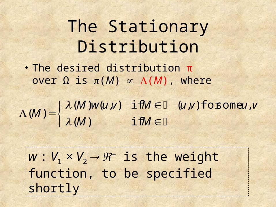
The Stationary Distribution

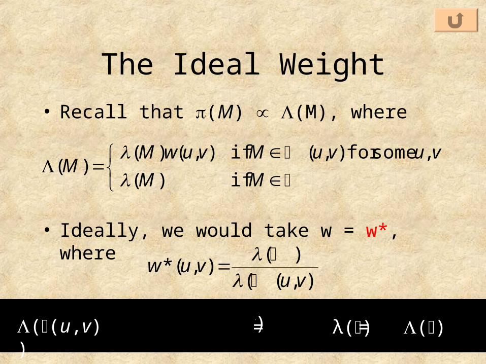
• The desired distribution π over Ω is (M) (M), where

MM

vuvuMvuwMM

if)(

, somefor ),( if),()()(

w : V1 × V2 + is the weight function, to be specified shortly

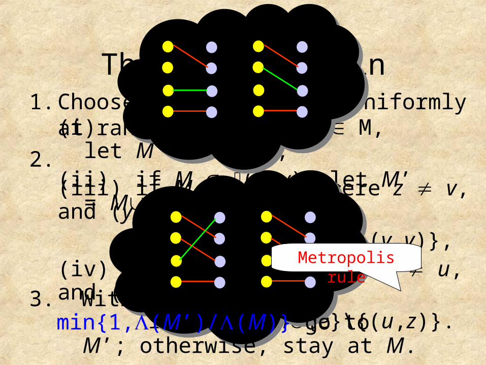
The Markov Chain1. Choose an edge e=(u,v) uniformly at random.

2. (i) If M and e M, let M’ = M\{e},(ii) if M (u,v), let M’ = M{e},

(iii) if M (u,z) where z v, and (y,v) M, let M’ = M{e}\{(y,v)},(iv) if M (y,v) where y u, and (u,z) M, let M’ = M{e}\{(u,z)}.

Metropolis rule

3. With probability min{1,(M’)/(M)} go to M’; otherwise, stay at M.

The Markov Chain (cont.)

• Finally, we add a self-loop probability of ½ to every state.

• This insures the MC is aperiodic.

• We also have irreducibility.

Detailed Balance

• Consider two adjacent matchings M and M’ with (M) ≤ (M’).

(M)P(M, M’) = (M’)P(M’, M)

P(M,M’) > 0

=: Q(M,M’)

)(M

(M)

mMMP

mMMP

'π

π1

2

1),'(

1

2

1)',(

• The transition probabilities between M and M’ may be written

mMM

2))'(),(min(

The Ideal Weight

• Recall that (M) (M), where

• Ideally, we would take w = w*, where

MM

vuvuMvuwMM

if)(

, somefor ),( if),()()(

)),(()(

),(*vu

vuw

((u,v))

),( vuM

(M) )),(()),((

)(vu

vu

λ(M)w(u,v)

),(

)(),(vuM

Mvuw

= λ() = ()

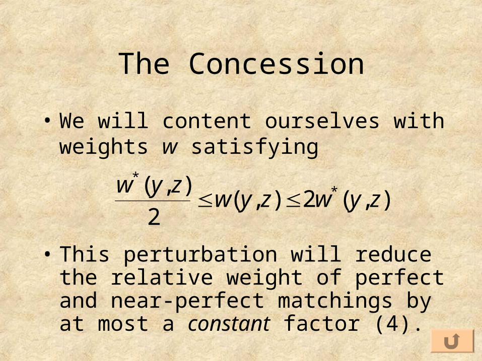
The Concession

• We will content ourselves with weights w satisfying

),(2),(2

),( **

zywzywzyw

• This perturbation will reduce the relative weight of perfect and near-perfect matchings by at most a constant factor (4).

The Mixing Time Theorem

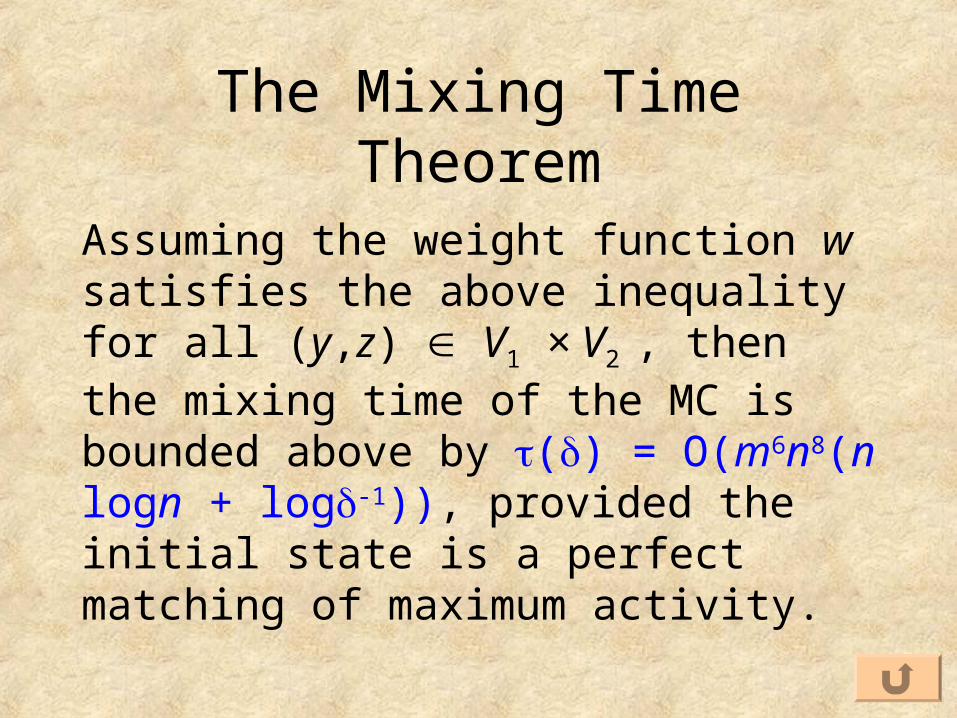
Assuming the weight function w satisfies the above inequality for all (y,z) V1 × V2 , then the mixing time of the MC is bounded above by () = O(m6n8(n logn + log-1)), provided the initial state is a perfect matching of maximum activity.

Edge Weights Revisited

• We will work with the complete graph on n+n vetices.

• Think of non-edges e E as having a very small activity of 1/n!.

• The combined weight of all invalid matchings is at most 1.

• We begin with activities whose ideal weights w* are easy to compute, and progress towards our target activities.

≡ 1*(e) = 1/n! for all e E*(e) = 1/n! for all e E

Step I

• We assume at the beginning of the phase w(u,v) approximates w*(u,v) within ratio 2 for all (u,v).

• Before updating an activity, we will find for each (u,v) a better approximation, one that is within ratio c for some 1 < c < 2.

• For this purpose we use the identity

)(π)),((π

),(*),(

vu

vuwvuw

)(),()),((

vuwvu

Step I (cont.)

• The mixing time theorem allows us to sample, in polynomial time, from a distribution ’ that is within variation distance of π.

• We choose = c1/n2, take O(n2 log -1) samples from ’, and use sample averages.

• Using a few Chernoff bounds, we have, with probability 1- (n2+1), approximation within ratio c to all of w*(u,v).

c1 > 0 is a sufficiently small constant

Step I (conclusion)

Taking c = 6/5 and using O(n2 log -1) samples, we obtain refined estimates w(u,v) satisfying

5w*(u,v)/6 ≤ w(u,v) ≤ 6w*(u,v)/5

Step II

• We update the activity of an edge e (e) ← (e) * exp(-1/2)

• The ideal weight function w* changes by at most a factor of exp(1/2).

• Since 6exp(1/2)/5 < 2, our estimates w after step I approximate w* within ratio 2 for the new activities.

≈ 1.978

Step II (cont.)

• We use the above procedure repeatedly to reduce the initial activities to the target activities.

≡ 1

*(e) = 1/n! for all e E*(e) = 1/n! for all e E

• This requires O(n2 · n log n) phases.• Each phase requires O(n2 log -1) samples.• Each sample requires O(n21 log n)

simulation steps (mixing time theorem). Overall time - O(n26 log2 n log -1)

The Error

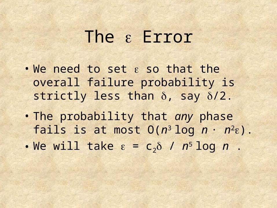
• We need to set so that the overall failure probability is strictly less than , say /2.

• The probability that any phase fails is at most O(n3 log n · n2).

• We will take = c2 / n5 log n .

Time Complexity

))loglog(( 122 nnnO

• Running time of generating a sample:

))log(loglog( 1226 nnnO

• Running time of the initialization:

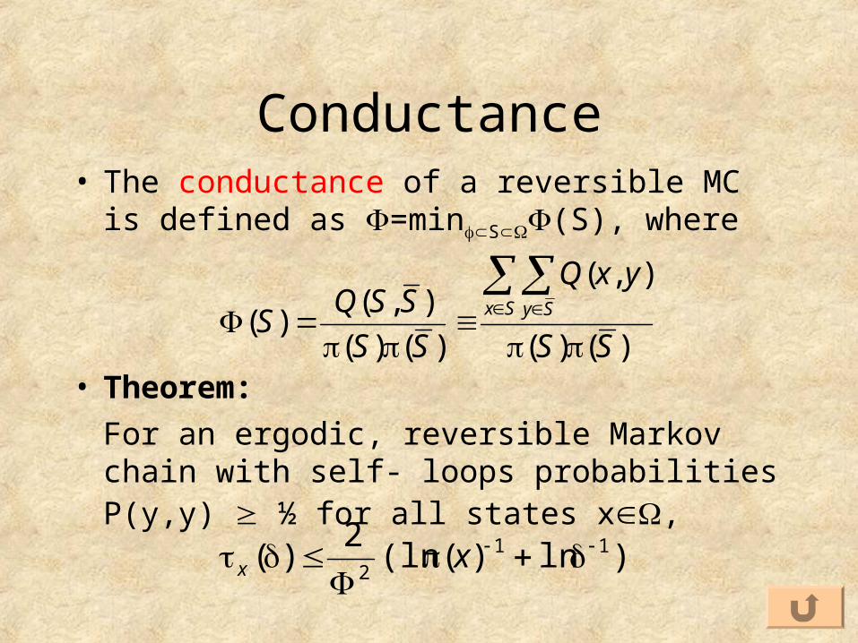
Conductance• The conductance of a reversible MC is defined as =minS(S), where

• Theorem:

For an ergodic, reversible Markov chain with self- loops probabilities P(y,y) ½ for all states x,

)()(

),(

)()(

),()(

SS

yxQ

SS

SSQS Sx Sy

)ln)((ln2

)( 112

xx

Canonical Paths

• We define canonical paths γI,F from all I Ω to all F .

• Denote Γ = { γI,F : (I, F) Ω × }.

• Certain transitions on a canonical path will be deemed chargeable.

• For each transition t denotecp(t) = {(I, F) : γI,F contains t as a chargeable

transition}

I F

• If I , then I F consists of a collection of alternating cycles.

• If I (y,z), then I F consists of a collection of alternating cycles together with a single alternating path from y to z.

y

z

Type A Path

• Assume I .

• A cycle v0 v1 … v2k = v0 is unwound by:

We assume w.l.g. that the edge (v0, v1) belongs to I

(i) removing the edge (v0, v1),

(ii) successively, for each 1 ≤ i ≤ k – 1, exchanging the edge (v2i, v2i+1) with (v2i-1, v2i),

(iii) adding the edge (v2k-1, v2k).• All these transitions are deemed chargeable.

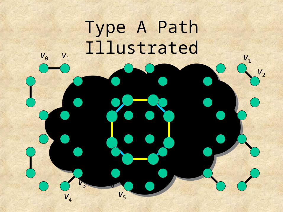
Type A Path Illustratedv0 v1 v1

v2

v4

v3

v5

v6

v0

v7

Type B Path

• Assume I (y,z).

• The alternating path y = v0 … v2k+1 = z is unwound by:(i) successively, for each 1 ≤ i ≤ k, exchanging the edge (v2i-1, v2i) with (v2i-2, v2i-1), and

(ii) adding the edge (v2k, v2k+1).

• Here, only the above transitions are deemed chargeable.

Type B Path Illustrated

y z

Congestion

• We define a notion of congestion of Γ:

• Lemma IAssuming the weight w approximates w* within ratio 2, then τ(Γ) ≤ 16m.

)(cp),(

)()()(

1max:)(

tFITt

FItQ

Lemma II

• Let u,y V1, v,z V2. Then,

(i) λ(u,v)λ((u,v)) ≤ λ(), for all vertices u,v with u v.

(ii) λ(u,v)λ((u,z))λ((y,v)) ≤ λ()λ((y,z)), for all distinct vertices u,v,y,z with u v.

• Observe that Mu,z My,v {(u,v)} decomposes into a collection of cycles together with an odd-length path O joining y and z.

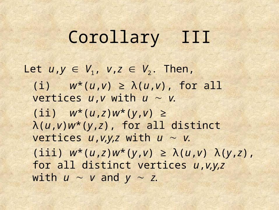
Corollary III

Let u,y V1, v,z V2. Then,

(i) w*(u,v) ≥ λ(u,v), for all vertices u,v with u v.

(ii) w*(u,z)w*(y,v) ≥ λ(u,v)w*(y,z), for all distinct vertices u,v,y,z with u v.

(iii) w*(u,z)w*(y,v) ≥ λ(u,v) λ(y,z), for all distinct vertices u,v,y,z with u v and y z.

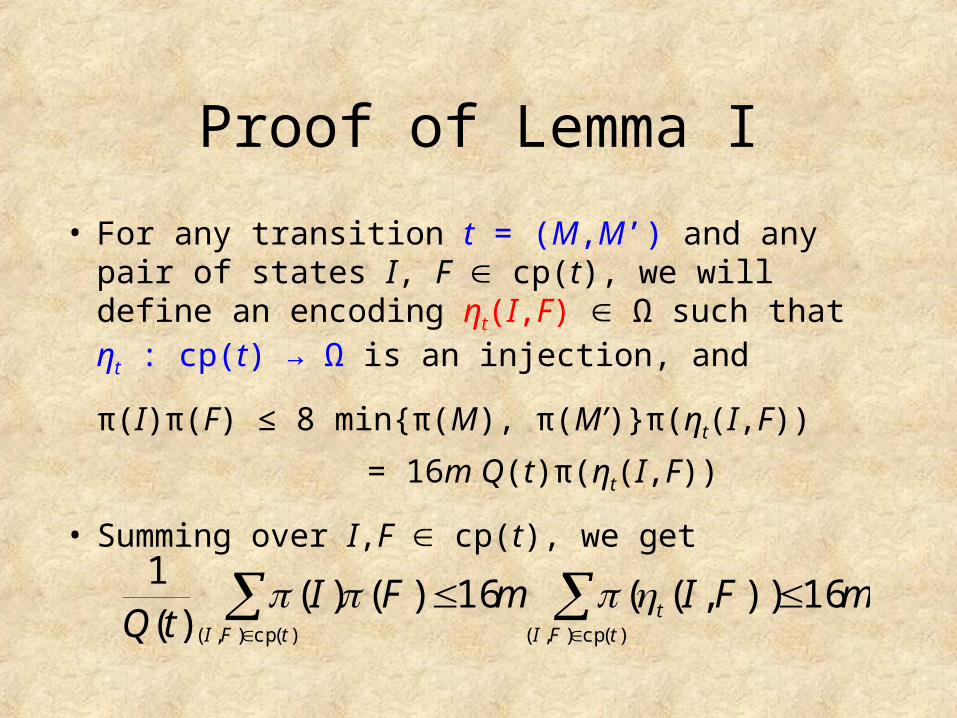
Proof of Lemma I

• For any transition t = (M,M’) and any pair of states I, F cp(t), we will define an encoding ηt(I,F) Ω such that ηt : cp(t) → Ω is an injection, and

π(I)π(F) ≤ 8 min{π(M), π(M’)}π(ηt(I,F))

= 16m Q(t)π(ηt(I,F))

• Summing over I,F cp(t), we get

mFImFItQ tFI

ttFI

16)),((16)()()(

1

)(cp),()(cp),(

The Injection ηt

• For a transition t = (M,M’) which is involved in stage (ii) of unwinding a cycle, the encoding is

ηt(I,F) = I F (M M’) \ {(v0, v1)}.

• Otherwise, the encoding is

ηt(I,F) = I F (M M’).

From Congestion to Conductance

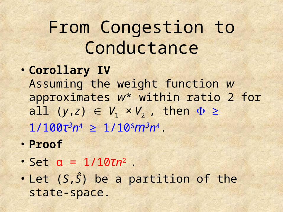
• Corollary IV Assuming the weight function w approximates w* within ratio 2 for all (y,z) V1 × V2 , then

≥ 1/100τ3n4 ≥ 1/106m3n4.

• Proof

• Set α = 1/10τn2 .

• Let (S,Ŝ) be a partition of the state-space.

Case I

• π(S ) / π(S) ≥ α and π(Ŝ ) / π(Ŝ) ≥ α.

• Just looking at canonical paths of type A we have a total flow of π(S )π(Ŝ ) ≥ α2π(S)π(Ŝ) across the cut.

• Thus, τQ(S,Ŝ) ≥ α2π(S)π(Ŝ), and,

(S) = Q(S,Ŝ)/π(S)π(Ŝ) ≥ α2 /τ = 1/100τ3n4.

1/10τn2

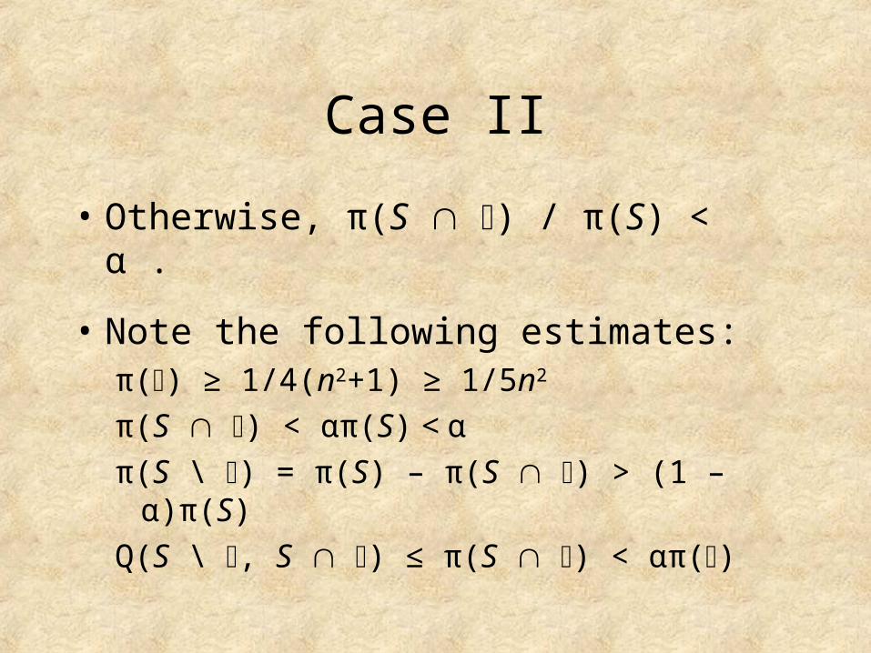
Case II

• Otherwise, π(S ) / π(S) < α .

• Note the following estimates:π() ≥ 1/4(n2+1) ≥ 1/5n2

π(S ) < απ(S) < α

π(S \ ) = π(S) – π(S ) > (1 – α)π(S)

Q(S \ , S ) ≤ π(S ) < απ()

Case II (cont.)

• Consider the cut (S \ , Ŝ ).

• The weight of canonical paths (all chargeable as they cross the cut) is π(S \ )π() ≥ (1 – α)π(S)/5n2 ≥ π(S)/6n2.

1/10τn2

• Hence, τQ(S \ ,Ŝ ) ≥ π(S)/6n2.

• Q(S,Ŝ) ≥ … ≥ π(S)π(Ŝ)/15τn2. (S) = Q(S,Ŝ)/π(S)π(Ŝ) ≥ 1/15τn2.

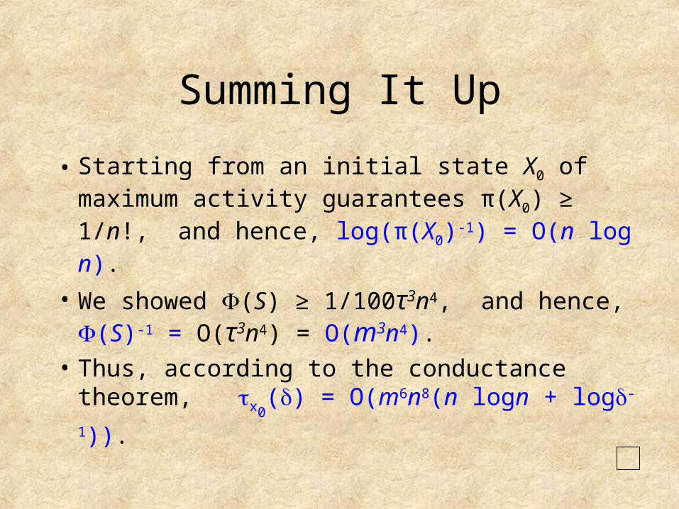
Summing It Up

• Starting from an initial state X0 of maximum activity guarantees π(X0) ≥ 1/n!, and hence, log(π(X0)-1) = O(n log n).

• We showed (S) ≥ 1/100τ3n4, and hence, (S)-1 = O(τ3n4) = O(m3n4).

• Thus, according to the conductance theorem, x0

() = O(m6n8(n logn + log-1)).