APPROVAL SHEET

Title of Thesis: System of Bound Particles for Interactive Flow Visualization

Name of Candidate: Jonathan Willard DeckerMaster of science, 2007

Thesis and Abstract Approved:Dr. Marc OlanoAssistant ProfessorDepartment of Computer Science andElectrical Engineering

Date Approved:

Curriculum Vitae

Name: Jonathan Willard Decker.

Permanent Address: 2509 Whitt Road, Kingsville Maryland, 21087.

Degree and date to be conferred: Master of Science, December 2007.

Date of Birth: March 29th, 1983.

Place of Birth: Baltimore.

Secondary Education: Fallston High, Bel Air, Maryland.

Collegiate institutions attended:

University of Maryland Baltimore County, Bachelor of Science Computer Science,2006.

Major: Computer Science.

Honors: Member of Phi Beta Kappa.

Professional positions held:

UMBC, Teaching Assistant for CMSC 341: Data Structures. (September 2007 –December 2007).UMBC, Independent Study under Dr. Penny Rheingans - developed an artist visu-alization for Kathy Marmor. (February 2006 – August 2006).

ABSTRACT

Title of Thesis: System of Bound Particles for Interactive Flow Visualization

Jonathan Willard Decker, Master of Science, 2007

Thesis directed by: Dr. Marc Olano, Assistant ProfessorDepartment of Computer Science andElectrical Engineering

Vector fields are complex data sets used by a variety of research fields. They contain

directional information at every point in space, and thus simply rendering one as a body of

vectors to a screen obfuscates any inherent meaning. One common method for visualizing

this data is particle tracing, where a large numbers of particles are placed and transported

through the field. This method simulates real experiments on fluid and storms, where the

probes provide a speckled outline of features of interest. However, since particles are sim-

ply points in space, the effect is closer to that of casting a dye into the flow. We are not

able to perceive the 3D formation of the mixed elements without observing the flow from

several directions at once. We present a particle system where each individual element is

actually a series of bound particles that move together as one, and can be rendered together

as complex shapes. By deploying these probes into a field, the effect of the flow on the

structure of each element as well as its rotation enables the viewer to immediately observe

the characteristics of the flow field. This includes complex features such as vortices, visi-

ble in the tumbling behavior of the probes through the field. We enhance this visualization

by providing various schemes of surface shading to express interesting information. We

demonstrate our method on steady and unsteady flow fields, and provide evaluation by an

domain expert.

System of Bound Particles for Flow Visualization

by

Jonathan Willard Decker

Thesis submitted to the Faculty of the Graduate Schoolof the University of Maryland in partial fulfillment

of the requirements for the degree ofMaster of Science

2007

c© Copyright Jonathan Willard Decker 2007

ACKNOWLEDGMENTS

Many thanks to Lynn Sparling, for providing the hurricane data used in this work, for

her expert advice, and domain knowledge that enabled our evaluation.

To Sarah for her love and encouragement, to my family for their support, and to ev-

eryone in the VANGOGH lab for putting up with me.

ii

TABLE OF CONTENTS

ACKNOWLEDGMENTS . . . . . . . . . . . . . . . . . . . . . . . . . . . . . ii

LIST OF FIGURES . . . . . . . . . . . . . . . . . . . . . . . . . . . . . . . . v

LIST OF TABLES . . . . . . . . . . . . . . . . . . . . . . . . . . . . . . . . . viii

Chapter 1 OVERVIEW . . . . . . . . . . . . . . . . . . . . . . . . . . . 1

Chapter 2 BACKGROUND AND RELATED WORK . . . . . . . . . . . 6

2.1 Graphics Hardware . . . . . . . . . . . . . . . . . . . . . . . . . . . . . . 6

2.1.1 General Purpose Graphics Hardware Programming . . . . . . . . . 8

2.2 Particle Systems . . . . . . . . . . . . . . . . . . . . . . . . . . . . . . . . 11

2.2.1 Particle Tracing . . . . . . . . . . . . . . . . . . . . . . . . . . . . 13

2.3 Mass Spring Systems . . . . . . . . . . . . . . . . . . . . . . . . . . . . . 16

Chapter 3 APPROACH . . . . . . . . . . . . . . . . . . . . . . . . . . . 21

3.1 Method Overview . . . . . . . . . . . . . . . . . . . . . . . . . . . . . . . 21

3.2 Initialization . . . . . . . . . . . . . . . . . . . . . . . . . . . . . . . . . . 23

3.3 Element Construction . . . . . . . . . . . . . . . . . . . . . . . . . . . . . 25

3.4 Particle Tracing . . . . . . . . . . . . . . . . . . . . . . . . . . . . . . . . 27

iii

3.5 Element Restoration . . . . . . . . . . . . . . . . . . . . . . . . . . . . . . 30

3.5.1 Texture Layout . . . . . . . . . . . . . . . . . . . . . . . . . . . . 32

3.6 Rendering and Surface Information . . . . . . . . . . . . . . . . . . . . . . 34

3.7 Background Volume Streaming . . . . . . . . . . . . . . . . . . . . . . . . 36

3.8 Application Interface . . . . . . . . . . . . . . . . . . . . . . . . . . . . . 37

Chapter 4 RESULTS AND EVALUATION . . . . . . . . . . . . . . . . . 39

4.1 Performance . . . . . . . . . . . . . . . . . . . . . . . . . . . . . . . . . . 39

4.2 Effectiveness . . . . . . . . . . . . . . . . . . . . . . . . . . . . . . . . . 41

4.3 Limitations . . . . . . . . . . . . . . . . . . . . . . . . . . . . . . . . . . 44

Chapter 5 CONCLUSION . . . . . . . . . . . . . . . . . . . . . . . . . . 47

5.1 Future Work . . . . . . . . . . . . . . . . . . . . . . . . . . . . . . . . . . 47

5.2 Conclusion . . . . . . . . . . . . . . . . . . . . . . . . . . . . . . . . . . 50

REFERENCES . . . . . . . . . . . . . . . . . . . . . . . . . . . . . . . . . . . 52

iv

LIST OF FIGURES

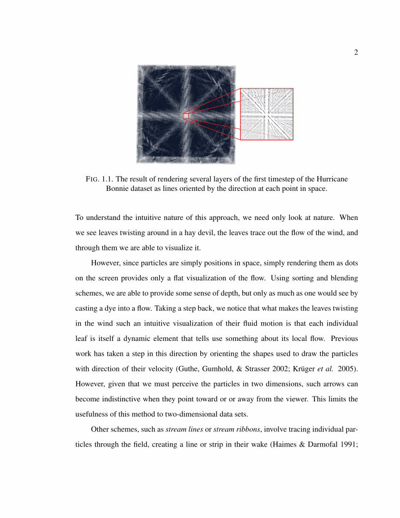
1.1 The result of rendering several layers of the first timestep of the Hurricane

Bonnie dataset as lines oriented by the direction at each point in space. . . 2

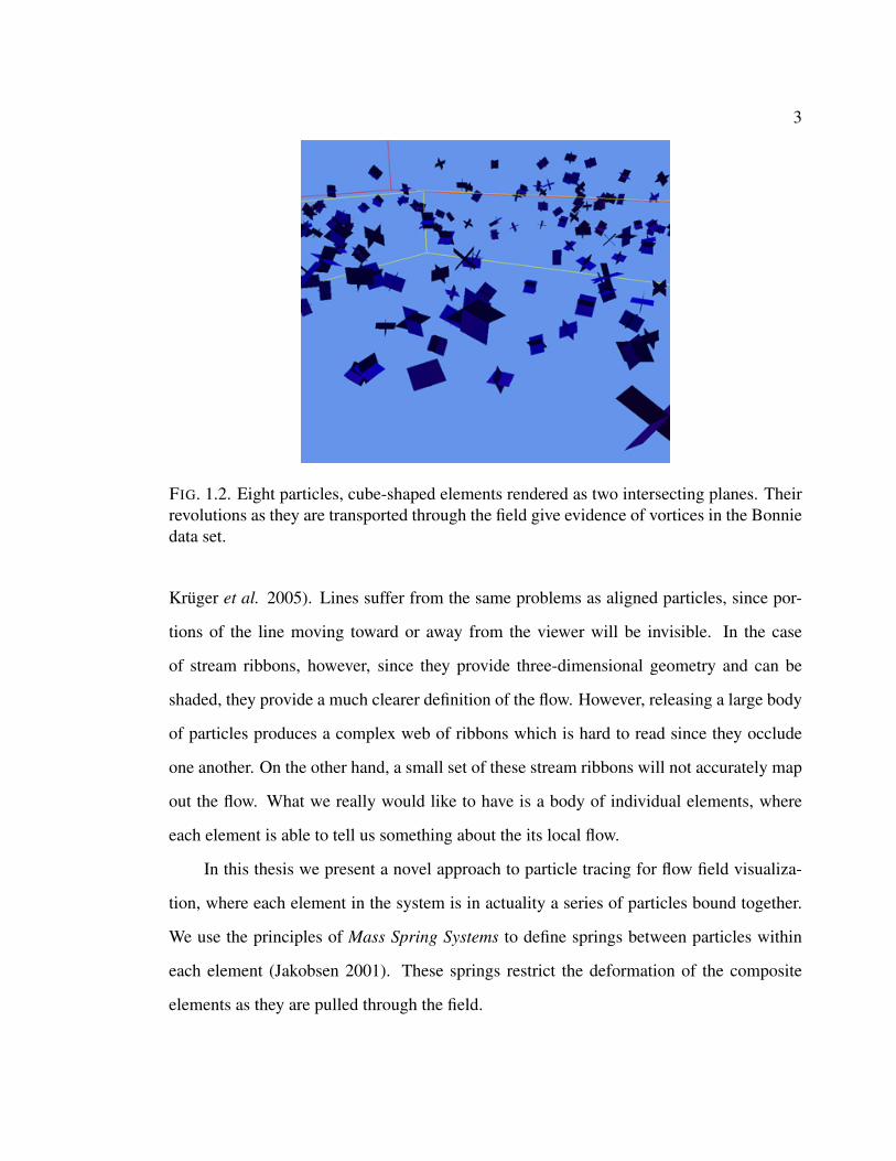
1.2 Eight particles, cube-shaped elements rendered as two intersecting planes.

Their revolutions as they are transported through the field give evidence of

vortices in the Bonnie data set. . . . . . . . . . . . . . . . . . . . . . . . . 3

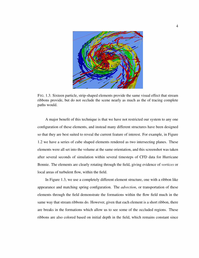
1.3 Sixteen particle, strip-shaped elements provide the same visual effect that

stream ribbons provide, but do not occlude the scene nearly as much as the

of tracing complete paths would. . . . . . . . . . . . . . . . . . . . . . . . 4

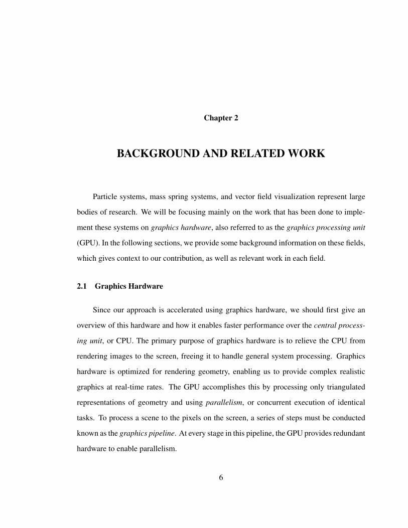
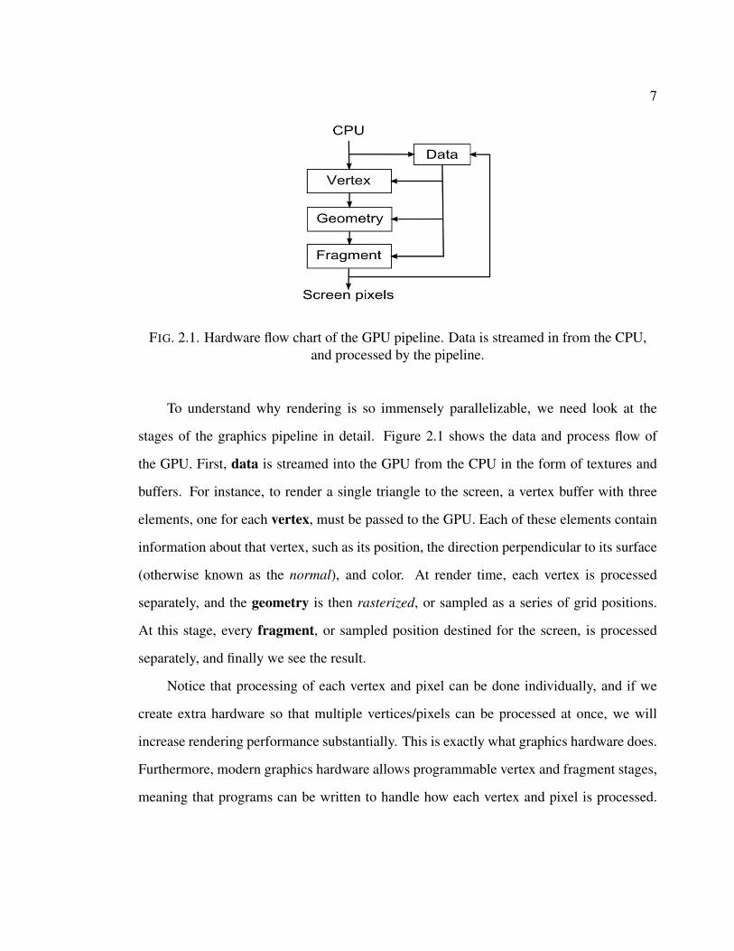
2.1 Hardware flow chart of the GPU pipeline. Data is streamed in from the

CPU, and processed by the pipeline. . . . . . . . . . . . . . . . . . . . . . 7

2.2 An illustration of utilizing graphics hardware to allow multiple iterations

over the same data within fragment programs. . . . . . . . . . . . . . . . . 9

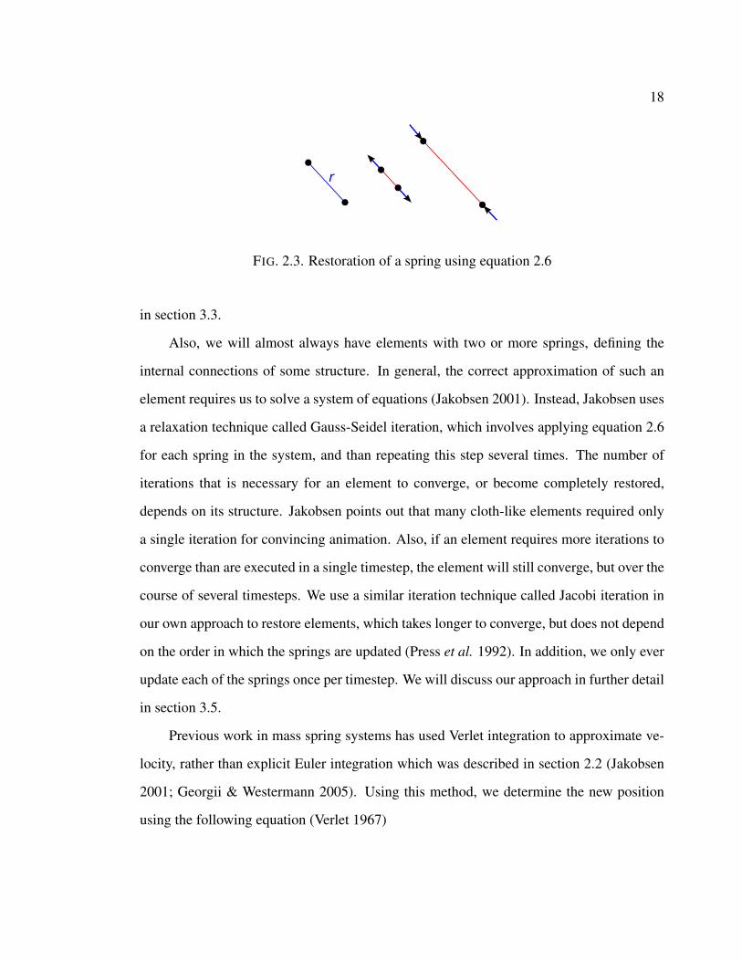
2.3 Restoration of a spring using equation 2.6 . . . . . . . . . . . . . . . . . . 18

3.1 A flow chart of our system. Thick gray lines with black arrows indicate

execute flow, while the thin black lines represent data flow. . . . . . . . . . 23

3.2 How the contains of the vertex and index buffers are organized using an

example of a four particle element. Numbers correspond to the id of the

particle, or which vertex it represents of the template shape. The index

buffer defines triangles within each element, in clockwise order. . . . . . . 24

v

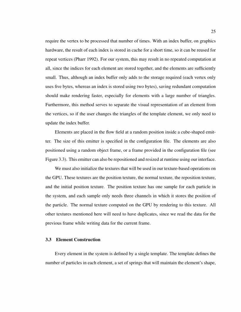
3.3 Elements are initialized in a cube emitter with a random (left) or a specified

(right) object frame. . . . . . . . . . . . . . . . . . . . . . . . . . . . . . 26

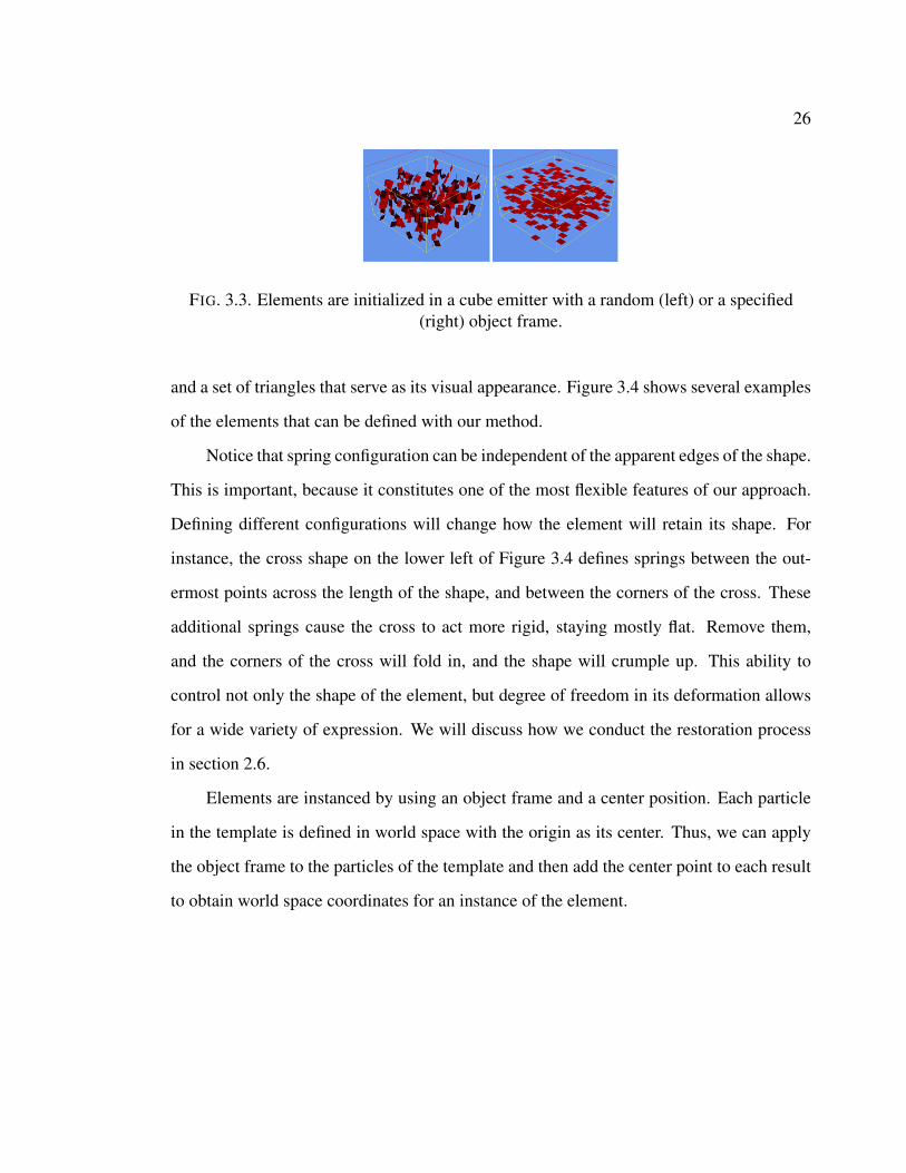
3.4 Some example elements possible in our system. On the left is the spring

configuration as it appears in the editor. On the right are the elements as

they appear in simulation. . . . . . . . . . . . . . . . . . . . . . . . . . . 27

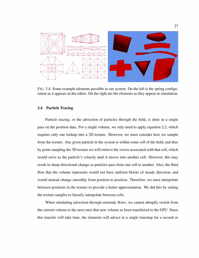
3.5 The blue line plots the altitude at each depth in the volume, scaled between

0 and 1. We approximate the inverse of this line so we can map the z

coordinate to the correct altitude in the volume stored linearly in the layers

of a 3D texture (represented by the pink line). The yellow line shows the

result of applying our approximation to the layer altitudes, which follows

the linearly increasing line closely. . . . . . . . . . . . . . . . . . . . . . 28

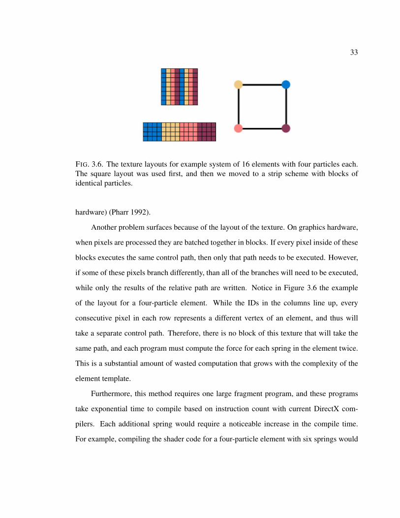
3.6 The texture layouts for example system of 16 elements with four particles

each. The square layout was used first, and then we moved to a strip scheme

with blocks of identical particles. . . . . . . . . . . . . . . . . . . . . . . 33

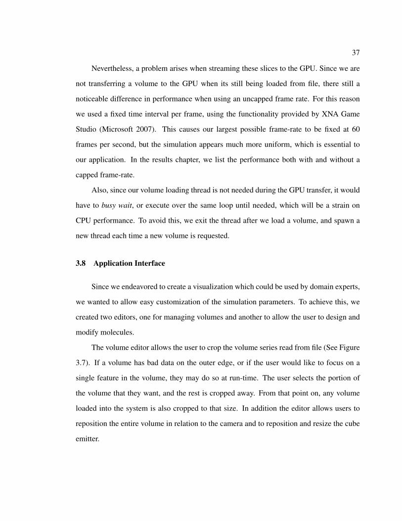
3.7 Outlines that identify the bounds in the system. The blue bounds represents

the bounds of the field, and the red bounds represents the field as it has

been cropped by the user, the yellow bounds are the bounds of the element

emitter. The pink bounds represent the size of a single cell in the volume. . 38

4.1 The change in frame rate as the number of elements in the system increases

exponentially for a element of fixed complexity (8-particle strip from Fig-

ure 3.4). The pink line shows the rates when the system is paused, the blue

line shows the rates for simulating one timestep of Hurricane Bonnie, and

the red line shows the rates for simulating multiple timesteps. . . . . . . . 40

vi

4.2 A visualization of shear vorticity in a synthetic field. There is constant

flow across each vertical layer, which varies as shown on the left. Three

frames are shown (viewed left to right) of 8-particle cube-shaped elements

advecting through this field. The upper elements (red) rotate clockwise and

the lower elements (blue) rotate counterclockwise. . . . . . . . . . . . . . 42

4.3 Several captures of a 16 particle strip-shaped element remaining straight

up within the eye of Hurricane Bonnie. . . . . . . . . . . . . . . . . . . . 43

4.4 Since an element are not replaced until its center is outside the bounds,

particles will drop outside the volume where velocity is not defined. These

particles receive the same velocity as the last layer, causing the outer por-

tion of each element to appear to drag. . . . . . . . . . . . . . . . . . . . . 45

5.1 An illustration of using a single particle spring configuration to simulate

sheet elements like the one shown on the right. To the left is a position

texture broken up into four blocks. Each particle looks up in the eight

positions around it in the texture, receiving force from only those particles

in its texture block. . . . . . . . . . . . . . . . . . . . . . . . . . . . . . . 48

vii

LIST OF TABLES

4.1 Performance on a single volume. Frames per second are given for

fixed/variable frame intervals. The columns represent the element count

for each run, and the rows represent the element complexity, which is dis-

played in the format: particles(triangles)[springs]. . . . . . . . . . . . . . . 40

viii

Chapter 1

OVERVIEW

Vector fields, or flow fields, are volumes of data that specify the direction and mag-

nitude of the flow at every point in space. Flow fields are often generated using Compu-

tational Fluid Dynamics (CFD), and are used in a number of fields, such as aeronautics

and storm identification. These fields are often quite large, sampling millions of positions

in space (See Fig. 1.1). This problem is compounded by the fact that in many cases, such

as with hurricane wind data, the velocity at each point in space varies over time. In these

cases, one vector field, which approximates what is called a steady flow, does not accu-

rately describe the flow. We need a sequence of vector fields, sampling a timeline of flow

at each point in space. This is what is known as an unsteady flow. Clearly such large sets

of data require advanced visualization techniques before their usefulness can be realized.

There has been a vast amount of work in flow field visualization. One area of research,

selective visualization is based on the insight that we need only show those parts of the

volume that are potentially of interest. Determining these features has been attempted

using a number of techniques, and we discuss some of these in the related work section.

The one of main interest to this thesis is particle tracing (Haimes & Darmofal 1991; van

Wijk 1992). This solution comes from that of real experiments on fluid and wind, and uses

the transportation of particles, or points in space, through the field to demonstrate the flow.

1

2

FIG. 1.1. The result of rendering several layers of the first timestep of the HurricaneBonnie dataset as lines oriented by the direction at each point in space.

To understand the intuitive nature of this approach, we need only look at nature. When

we see leaves twisting around in a hay devil, the leaves trace out the flow of the wind, and

through them we are able to visualize it.

However, since particles are simply positions in space, simply rendering them as dots

on the screen provides only a flat visualization of the flow. Using sorting and blending

schemes, we are able to provide some sense of depth, but only as much as one would see by

casting a dye into a flow. Taking a step back, we notice that what makes the leaves twisting

in the wind such an intuitive visualization of their fluid motion is that each individual

leaf is itself a dynamic element that tells use something about its local flow. Previous

work has taken a step in this direction by orienting the shapes used to draw the particles

with direction of their velocity (Guthe, Gumhold, & Strasser 2002; Kruger et al. 2005).

However, given that we must perceive the particles in two dimensions, such arrows can

become indistinctive when they point toward or or away from the viewer. This limits the

usefulness of this method to two-dimensional data sets.

Other schemes, such as stream lines or stream ribbons, involve tracing individual par-

ticles through the field, creating a line or strip in their wake (Haimes & Darmofal 1991;

3

FIG. 1.2. Eight particles, cube-shaped elements rendered as two intersecting planes. Theirrevolutions as they are transported through the field give evidence of vortices in the Bonniedata set.

Kruger et al. 2005). Lines suffer from the same problems as aligned particles, since por-

tions of the line moving toward or away from the viewer will be invisible. In the case

of stream ribbons, however, since they provide three-dimensional geometry and can be

shaded, they provide a much clearer definition of the flow. However, releasing a large body

of particles produces a complex web of ribbons which is hard to read since they occlude

one another. On the other hand, a small set of these stream ribbons will not accurately map

out the flow. What we really would like to have is a body of individual elements, where

each element is able to tell us something about the its local flow.

In this thesis we present a novel approach to particle tracing for flow field visualiza-

tion, where each element in the system is in actuality a series of particles bound together.

We use the principles of Mass Spring Systems to define springs between particles within

each element (Jakobsen 2001). These springs restrict the deformation of the composite

elements as they are pulled through the field.

4

FIG. 1.3. Sixteen particle, strip-shaped elements provide the same visual effect that streamribbons provide, but do not occlude the scene nearly as much as the of tracing completepaths would.

A major benefit of this technique is that we have not restricted our system to any one

configuration of these elements, and instead many different structures have been designed

so that they are best suited to reveal the current feature of interest. For example, in Figure

1.2 we have a series of cube shaped elements rendered as two intersecting planes. These

elements were all set into the volume at the same orientation, and this screenshot was taken

after several seconds of simulation within several timesteps of CFD data for Hurricane

Bonnie. The elements are clearly rotating through the field, giving evidence of vortices or

local areas of turbulent flow, within the field.

In Figure 1.3, we use a completely different element structure, one with a ribbon like

appearance and matching spring configuration. The advection, or transportation of these

elements through the field demonstrate the formations within the flow field much in the

same way that stream ribbons do. However, given that each element is a short ribbon, there

are breaks in the formations which allow us to see some of the occluded regions. These

ribbons are also colored based on initial depth in the field, which remains constant since

5

the data shown here provides only two dimensional vectors.

While springs in our systems are intended for restricting shape of the individual ele-

ments, interesting things are possible when we define springs between particles in different

elements. In this way we are able to connect all the elements in the system, creating what

we call super sets. We demonstrate a few uses of these larger structures and discuss further

directions for them in the conclusion chapter.

We implemented our application using XNA Game Studio, which is a high-level

graphics API for C# which encapsulates most of the features provided by Direct3D (Di-

rectX 9) (Microsoft 2007). However, the overhead of using a language which runs in a

virtual machine should not affect overall performance, since we utilize the graphics pro-

cessing unit (GPU) to accelerate the major operations necessary to our approach. This in-

cludes the transportation of the particles through the field and the restoration of the springs

between particles. The GPU provides parallel architecture, or redundant hardware which

allows for concurrent execution of identical tasks. Since we can apply operations to each

particle individually, we can process many particles at once using this hardware. In this

way we are able to simulate a large number of composite particle elements at real-time

rates, and in a manner that is not bounded by the CPU.

In the following chapters we provide further details into our approach, including back-

ground information on the relevant topics. We also provide evaluation by a domain expert

in its effectiveness on feature extraction within hurricane data.

Chapter 2

BACKGROUND AND RELATED WORK

Particle systems, mass spring systems, and vector field visualization represent large

bodies of research. We will be focusing mainly on the work that has been done to imple-

ment these systems on graphics hardware, also referred to as the graphics processing unit

(GPU). In the following sections, we provide some background information on these fields,

which gives context to our contribution, as well as relevant work in each field.

2.1 Graphics Hardware

Since our approach is accelerated using graphics hardware, we should first give an

overview of this hardware and how it enables faster performance over the central process-

ing unit, or CPU. The primary purpose of graphics hardware is to relieve the CPU from

rendering images to the screen, freeing it to handle general system processing. Graphics

hardware is optimized for rendering geometry, enabling us to provide complex realistic

graphics at real-time rates. The GPU accomplishes this by processing only triangulated

representations of geometry and using parallelism, or concurrent execution of identical

tasks. To process a scene to the pixels on the screen, a series of steps must be conducted

known as the graphics pipeline. At every stage in this pipeline, the GPU provides redundant

hardware to enable parallelism.

6

7

FIG. 2.1. Hardware flow chart of the GPU pipeline. Data is streamed in from the CPU,and processed by the pipeline.

To understand why rendering is so immensely parallelizable, we need look at the

stages of the graphics pipeline in detail. Figure 2.1 shows the data and process flow of

the GPU. First, data is streamed into the GPU from the CPU in the form of textures and

buffers. For instance, to render a single triangle to the screen, a vertex buffer with three

elements, one for each vertex, must be passed to the GPU. Each of these elements contain

information about that vertex, such as its position, the direction perpendicular to its surface

(otherwise known as the normal), and color. At render time, each vertex is processed

separately, and the geometry is then rasterized, or sampled as a series of grid positions.

At this stage, every fragment, or sampled position destined for the screen, is processed

separately, and finally we see the result.

Notice that processing of each vertex and pixel can be done individually, and if we

create extra hardware so that multiple vertices/pixels can be processed at once, we will

increase rendering performance substantially. This is exactly what graphics hardware does.

Furthermore, modern graphics hardware allows programmable vertex and fragment stages,

meaning that programs can be written to handle how each vertex and pixel is processed.

8

Thus we have a very streamlined architecture optimized for graphics rendering, but also

robust enough to handle a vast number of rendering techniques.

There is also a geometry step in-between these stages which produces the triangles

from the vertices. This stages has only become programmable in recent graphics hardware

(NVIDIA Corporation 2006). For the purposes of a particle system, the geometry stage

provides a means for rendering simple particles as simple geometry. This feature is known

as point sprites, where, for each vertex, the GPU creates a quadrilateral with two triangles

centered at the vertex position, and aligned to the screen. These primitives can then be

textured in a fragment program, using provided texture coordinates.

While this architecture is meant specifically for rendering, it is simple to see how

many parallel algorithms, or algorithms that can be broken up into independent tasks and

executed at the same time, could also benefit from its performance.

2.1.1 General Purpose Graphics Hardware Programming

Since graphics hardware is significantly faster than CPUs and is widely available, it

would be advantageous if we could map computationally heavy algorithms to the GPU.

However, until recently, vendors of graphics hardware have not incorporated special hard-

ware to allow programmers to run general purpose algorithms. Therefore, in order to utilize

this hardware for such algorithms, the data and operations involved must be mapped to the

graphics pipeline. In general, efficiently mapping of an algorithm onto graphics hardware

requires use of a collection of standard ”tricks” which are common to applications which

perform General Purpose computation on GPUs (GPGPU) (Owens et al. 2005). Much

work already exists in this field, and a number of algorithms of interest to a wide vari-

ety of fields have been implemented in this way, incurring large speedups from their CPU

counterparts.

The most common means of doing this is often referred to as a texture-based scheme

9

FIG. 2.2. An illustration of utilizing graphics hardware to allow multiple iterations overthe same data within fragment programs.

for a given algorithm (Figure 2.2). The main idea is to use concurrent fragment programs

to handle independent subproblems of a parallel algorithm. This method stores the data

related to every subproblem at each position in a texture. The ordinary purpose of a texture

is to store image data that is displayed on the surface of geometry. Each element in the

texture corresponds to a color in the image, and how these textures map to geometry is

defined by texture coordinates present at each vertex. However, for the purpose of the

texture-based GPGPU scheme, a texture is used to store general data we wish to have some

algorithm iterate upon. This data is limited to a set of one to four elements per texture,

since this is the range provided in textures. The precision of these elements can vary from

one byte each to single-precision floating point.

Now we have a texture that represents an array of input data, with one set of values

for each subproblem of the algorithm. To complete one iteration of the algorithm, we must

iterate over each element in this array, and produce a new array of data which constitutes

the output of the iteration. To model this process with textures on the GPU, we must render

10

a screen-aligned quadrilateral which is exactly the same size as the texture filled with input

data. After the shape is rasterized, one pixel will exist for each position in the texture. To

provide access to those texture positions at each pixel, we define texture coordinates for the

vertices of the quadrilateral so that the texture positions line up with the pixel positions.

Each fragment program then reads a texture ”color” which corresponds to the input data,

and runs an algorithm on it to produce a new iteration of that data. This new data is used as

the pixel color that is drawn to the render target.

The final result of rendering the quadrilateral is a new iteration of the data in the input

texture at the render target, which is set to be another texture. To handle the next iteration,

we switch out the texture we used as input to the fragment programs with the texture used

as the render target. This scheme allows for the implementation of parallel algorithms

such as sorting (Kruger et al. 2005; Latta 2004), and also for solving large numbers of

independent instances of the same equation, such as with the velocity integration schemes

used in particle tracing discussed later (Telea & van Wijk 2003; Kruger et al. 2005).

One of the major limitations of GPU accelerated implementations is that the results of

the computation are in the framebuffer on the GPU. We must transfer this data back to the

CPU before we can have access to the information. This is a problem because the band-

width between the CPU and the GPU is significantly less than the speed obtained through

memory access, and will thus become a bottleneck in the any applications attempting to

make this transfer continuously. Our approach avoids this limitation by using the data

produced by our general purpose computation to render geometry.

Recently NVIDIA has created a framework for general purpose application of their

hardware called Compute Unified Device Architecture (CUDA) (NVIDIA Corporation

2007). CUDA is only available on CUDA-enabled GPUs, and allows programmers to

write C-like code which will run in a parallelized fashion on the GPU. While this capabil-

ity could replace the texture-based methods for most applications, the original method is

11

still more viable for systems that use the results of GPU computation to render geometry.

Many algorithms in a variety of fields have been implemented for execution on pro-

grammable graphics hardware. In the following sections related to our work we discuss

some research that utilizes graphics hardware to accelerate general purpose algorithms.

2.2 Particle Systems

Particle systems are used to simulate a wide variety of complex phenomena which can-

not easily be represented with geometry and texturing. The use of these systems for mod-

eling various special effects such as fire and smoke was first explored by Reeves (Reeves

1983). More recently, particle systems have been implemented which operate almost ex-

clusively in fragment programs on the graphics hardware, thus enabling them to iterate over

a large number of particles at real-time frame-rates (Kipfer, Segal, & Westermann 2004;

Kolb, Latta, & Rezk-Salama 2004).

In a particle system, the individual elements are indistinct and their global motion

creates a desired effect. The information at each particle is position and velocity, as well as

various surface attributes such as color. Particles are normally stored together in a single

array to allow fast traversal and avoid the overhead of dynamic data creation. The position

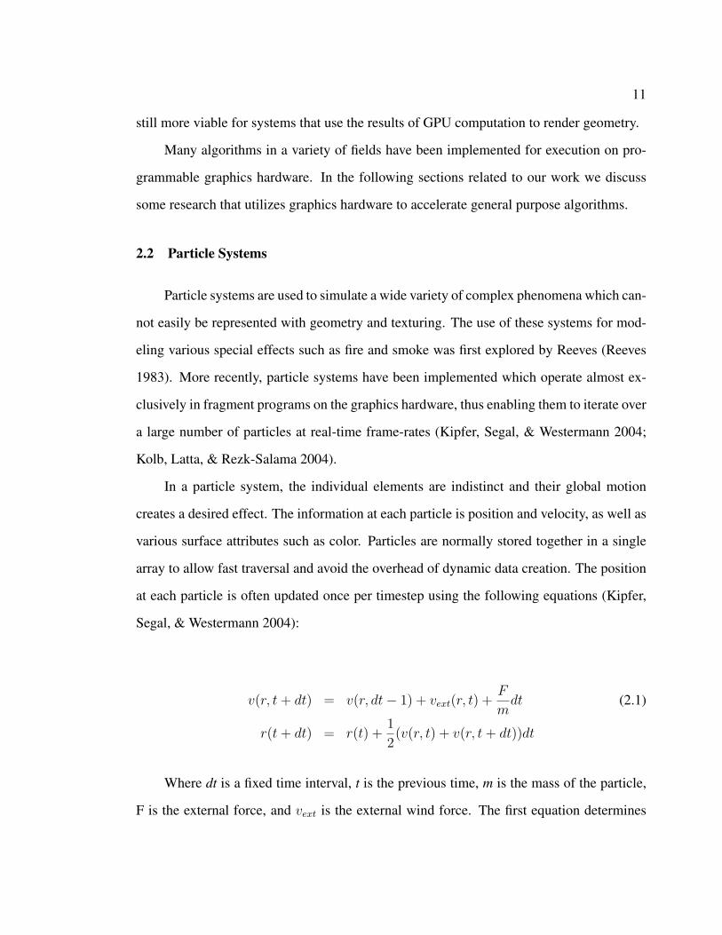
at each particle is often updated once per timestep using the following equations (Kipfer,

Segal, & Westermann 2004):

v(r, t + dt) = v(r, dt− 1) + vext(r, t) +F

mdt (2.1)

r(t + dt) = r(t) +1

2(v(r, t) + v(r, t + dt))dt

Where dt is a fixed time interval, t is the previous time, m is the mass of the particle,

F is the external force, and vext is the external wind force. The first equation determines

12

the new velocity v of the particle and the second equation finds the new position r. This

is known as explicit Euler integration, and is one integration method used to approximate

the velocity of each particle. This velocity is dependent on various factors, such as gravity

and response to collision, as well as the external wind force. In our work, we focus on the

vext force alone, for which we use a variation of this integration technique which we will

describe in section 2.2.1.

Most particle systems also maintain particle lifecycles. Particles are first initialized at

an emitter, or source, which can be a single point or other shapes such as a line or a cube.

These particles are then moved about the scene using equation 2.2. Furthermore, a lifetime

value is stored for each particle, and decremented at each timestep. Once a particle has

reached the end of its lifetime, it is repositioned at the emitter. For systems with explicit

velocity, this too must be initialized at rebirth.

Kipfer et al. proposed one of the best known completely hardware-accelerated par-

ticle systems, so called Uberflow (Kipfer, Segal, & Westermann 2004). This system uses

equation 2.2 to update particles based on gravity, terrain collision, and particle-to-particle

collision. This is done in fragment programs using the texture-based method described in

section 2.1.1. Terrain collision was done by simply comparing the depth of a particle to the

values in a height map. However, to simulate particle-to-particle collisions we would need

to exhaustively compare all particles in the system. Kipfer et al. avoided this by identifying

neighboring particles that are possible candidates for collision response. This was done by

sorting the particles by cell location using a texture-based sort. In our work, we decided not

to include collision detection, since our goal was the visualization of fluid flow and rather

than the simulation of physical bodies.

A problem surfaces when we wish to render the particles. The information about the

position of each particle is in GPU memory. Kipfer et al. use an OpenGL graphics API

feature called Superbuffers to repurpose the position texture, which stores the positions of

13

the particles in the color channels at each position in the texture, as a vertex buffer storing

one position per vertex. This method is used by a number of researchers in this field,

including Kruger et al. and Telea et al., discussed in the following section (Kipfer, Segal,

& Westermann 2004; Kruger et al. 2005; Telea & van Wijk 2003). Another approach used

by Zeller for the NVIDIA cloth demo, which is available in the DirectX graphics API, is

called vertex texture fetch (VTF) (Zeller 2005; 2007). With this method, we look up the

position in the texture when we process each vertex, rather than reinterpreting texture data

as vertex data. We use VTF in our work, since our position data is not organized as it

should appear in a vertex buffer. For more details, please see Section 3.5.1.

Since Kipfer et al. also use alpha blending, where the alpha channel of the fragment

color denotes its opacity, they sort the particles by depth each frame before rendering. This

results in each particle appearing as a fuzzy speck, which greatly adds to the aesthetic

nature of the simulation while also making it easier to see the global motion through a

field. We do not use alpha blending in our approach to avoid the necessary sorting step, but

rather alpha test, which allows only for alpha values of 1 or 0 (visible and invisible).

Kolb et al. created a particle system much in the same vein as Kipfer et al. but

with collision detection against any model rather than just with a height field (Kolb, Latta,

& Rezk-Salama 2004). This was done using a series of depth slices, which allow fast

sampling to determine the distance a particle is from the object. It only works on static

scenes, and requires a pre-process to create the depth textures. Again, we are not interested

in this interaction, so these methods do not apply to our approach.

2.2.1 Particle Tracing

Since a particle system is such an elegant use of graphics hardware, much research

has explored its use in a variety of applications. One of the major applications that has

been investigated is fluid flow visualization. Researchers studying fluid flow determine

14

the values in these fields using computational fluid dynamics, a process that can take from

days to weeks (Bruckschen et al. 2001). While such data is of great interest in a number of

fields, such as hurricane prediction, it is very hard to visualize. This is immediately obvious

when you take into account the size of these data sets. These fields contain a direction and

magnitude at every sampled position, and in the case of 3D fields often sample millions

of points. Fluid flows that can be represented by just one of these fields is called a steady

flow, since the vector at each sampled position is always constant. Fluid flows where the

vectors at each point vary over time are called unsteady flows, and these are more common

in nature. Obviously we cannot simply render these vectors as a grid of compass needles,

since the result would be nearly impossible to interpret.

One possible solution is to use a selective visualization, which attempts to extract

important features from a dataset. We can do this by determining heuristics for finding

known features, but it is difficult to arrive at such heuristics. Another method is known as

particle tracing, which is inspired real simulations on fluids, where probes or tracer (dye)

is cast into the field in order to create a reference for its motion (Ottino 1988).

Particle tracing transports large bodies of massless particles through the field over

time (Kruger et al. 2005). The particles in the system are suspended within the field, if

they are transported out of bounds they are repositioned at the emitter. The advection, or

transportation of a particle, is found using the following equation:

r(t + dt) = r(t) + vext(r, t)dt (2.2)

This is a numerical integration of the velocity at position r known as implicit Euler

integration (Teitzel, Grosso, & Ertl 1997). vext is determined by interpolating between the

vectors located at the nearest sampled positions in the field. This can be done by using

tri-linear interpolation, or a linear blend in each dimension between cells in the field, to

15

determine the nearest vector in the flow field (Kruger et al. 2005). This is the advection

equation we use in our approach, and we will refer back often.

Jobard et al. presents one of the earliest hardware-accelerated examples of this

method, using a SGI Octane workstation to transport 65,000 particles through 2D unsteady

flows at two frames a second (Jobard, Erlebacher, & Hussaini 2000). Brusckschen et al.

took a different approach to this scheme, using per-calculated particle traces through 3D

vector fields in order produce an early real-time visualization of these traces at 60 frames

a second (Bruckschen et al. 2001). As graphics hardware improved, particle tracing in

real-time became more viable. Telea and Wijk proposed a system that advects particles

through the 2D and 3D field at interactive rates on GeForce 3 hardware (Telea & van Wijk

2003). This work renders particles as blurry comets, with tails fading out in the direction

they came, which expresses global movement as well as some indication of local motion at

each particle.

Kruger et al. utilizes the GPU to cast millions particles into a steady fluid flow at

real-time rates (Kruger et al. 2005). For advection, they use an additive integration scheme

called embedded Runge-Kutta. This scheme modifies the step size used for integration

based on estimated error. While this method is faster and more accurate than the Euler

approach (equation 2.2), according to Kruger et al., these advantages are not significant

enough to be noticeable in a visualization.

They rendered their particles in a number of ways, such as with spheres, alpha blended

point sprites, and flow-aligned arrows. In addition, they color the particles based on the

integration error produced by using Runge-Kutta. The addition of particles which reveal

their own local flow is noteworthy, since it gives the observer a clearer picture of what is

happening in a given region of the flow.

Kruger et al. demonstrate the use of several pre-existing techniques for visualizing the

life of individual particles over time. Instead of rendering particles at one point in space,

16

these techniques render each particle at every point it has existed at since initialization.

Stream lines are one such technique, where these points are rendered as a line (Haimes &

Darmofal 1991). Stream lines are more appropriate for 2D flows, since they do not convey

any information about depth. Stream ribbons, on the other hand, are rendered as 3D strips

and thus demonstrate the 3D motion of a particle over time (Hultquist 1992; Post & van

Walsum 1993). This provides a clear indication of the local motion of each particle through

3D space. We feel this is the most expressive technique proposed in previous work, and in

our approach we are able to mimic this using our composite particle elements.

2.3 Mass Spring Systems

Terzopoulos et al. pioneered the use of elasticity theory in computer graphics to sim-

ulate deformable bodies (Terzopoulos et al. 1987). They concluded in their work that the

dynamic nature of a deformable body combines the concepts of shape and motion, which is

essential to our work, since the composite elements are meant to emphasize motion. Since

this seminal work, research has been ongoing into finding the most efficient model for de-

formation, while still maintaining a desired level of accuracy. Several of these methods

are particle-based, such as meshless shape matching (Muller et al. 2005) and mass spring

systems (Jakobsen 2001).

A mass spring system defines springs, or elastic constraints, between the particle

which make up an object, such as a sheet of cloth (Jakobsen 2001). The idea is for the

spring to apply forces on its endpoints as a function of the amount it has stretched or

shrunk. Using Hooke’s law, the scalar force produced by a spring s is given by the follow-

ing equation:

Fs = kx (2.3)

17

Where k is a stiffness constant in the range [0,1] and x is the displacement from the

initial distance between the points. We will come back to k in a moment. To determine x

for a spring between the particles p1 and p2 with rest length r we compute:

x =||−−→p1p2|| − r

||−−→p1p2||(2.4)

Now we have the force acting on both particles, which we must apply to each point

separately, in the direction of the opposite point:

p′1 =

Fs(p1 − p2)

2(2.5)

p′2 =

−Fs(p1 − p2)

2

Figure 2.3 demonstrates this technique with a simple example. On the left, the spring

is already at rest, so no restoration forces are required. In the center, the two points have

come closer together, and thus Fs is positive, resulting in a repelling force at each particle.

In the right image, the points are too far apart, so Fs is negative and the points are moved

towards one another.

Thus, for one spring, all we need to do is apply equation 2.6 to its endpoints. How-

ever, we need to determine a good spring constant k for each spring within an element.

This can involve solving a series of nonlinear equations, or simply determining good val-

ues through experimentation. To avoid this, Jakobsen simple restricted his simulation to

infinitely stiff springs, which act as sticks within an element (Jakobsen 2001). While this

limits the amount of deformation possible within particle defined meshes, it allows a simple

means for general spring configuration. We use this method in our approach, since one of

our contributions is a system of customizable deformable elements. We discuss this further

18

FIG. 2.3. Restoration of a spring using equation 2.6

in section 3.3.

Also, we will almost always have elements with two or more springs, defining the

internal connections of some structure. In general, the correct approximation of such an

element requires us to solve a system of equations (Jakobsen 2001). Instead, Jakobsen uses

a relaxation technique called Gauss-Seidel iteration, which involves applying equation 2.6

for each spring in the system, and than repeating this step several times. The number of

iterations that is necessary for an element to converge, or become completely restored,

depends on its structure. Jakobsen points out that many cloth-like elements required only

a single iteration for convincing animation. Also, if an element requires more iterations to

converge than are executed in a single timestep, the element will still converge, but over the

course of several timesteps. We use a similar iteration technique called Jacobi iteration in

our own approach to restore elements, which takes longer to converge, but does not depend

on the order in which the springs are updated (Press et al. 1992). In addition, we only ever

update each of the springs once per timestep. We will discuss our approach in further detail

in section 3.5.

Previous work in mass spring systems has used Verlet integration to approximate ve-

locity, rather than explicit Euler integration which was described in section 2.2 (Jakobsen

2001; Georgii & Westermann 2005). Using this method, we determine the new position

using the following equation (Verlet 1967)

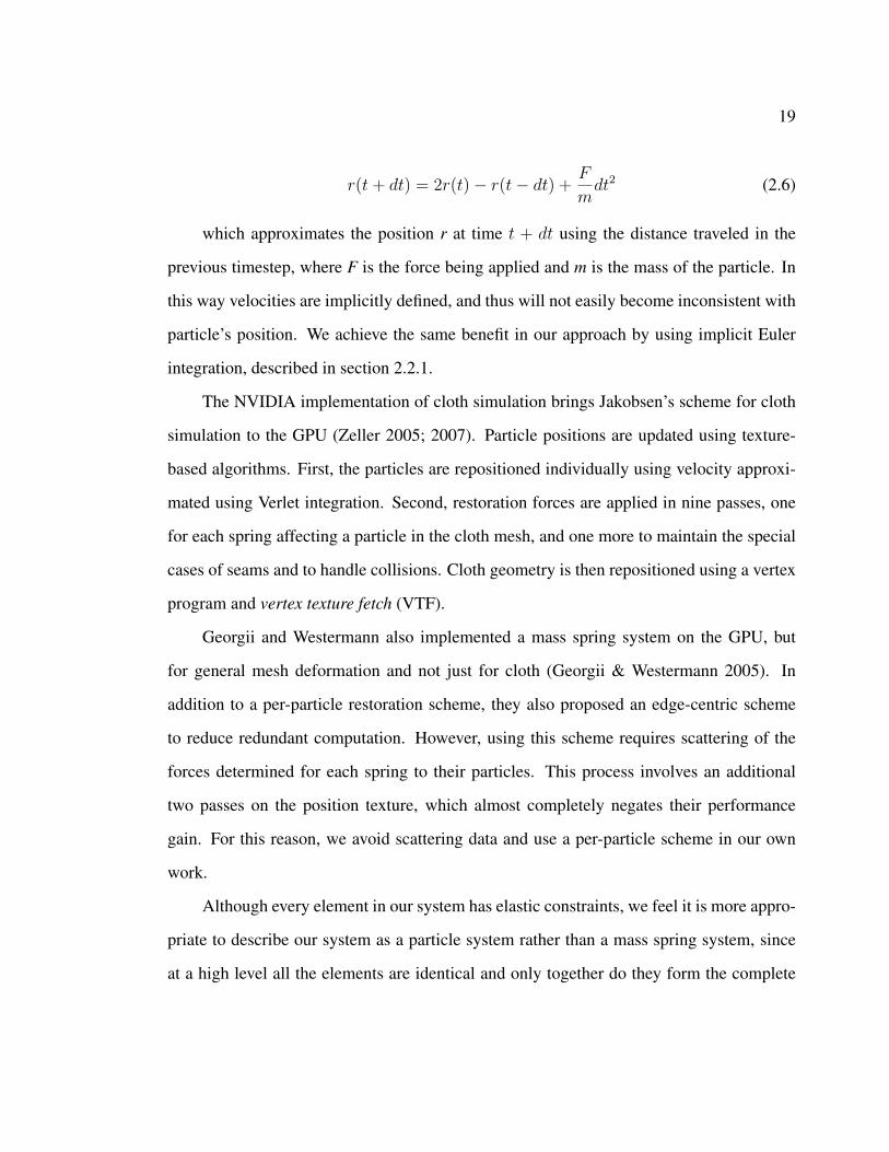
19

r(t + dt) = 2r(t)− r(t− dt) +F

mdt2 (2.6)

which approximates the position r at time t + dt using the distance traveled in the

previous timestep, where F is the force being applied and m is the mass of the particle. In

this way velocities are implicitly defined, and thus will not easily become inconsistent with

particle’s position. We achieve the same benefit in our approach by using implicit Euler

integration, described in section 2.2.1.

The NVIDIA implementation of cloth simulation brings Jakobsen’s scheme for cloth

simulation to the GPU (Zeller 2005; 2007). Particle positions are updated using texture-

based algorithms. First, the particles are repositioned individually using velocity approxi-

mated using Verlet integration. Second, restoration forces are applied in nine passes, one

for each spring affecting a particle in the cloth mesh, and one more to maintain the special

cases of seams and to handle collisions. Cloth geometry is then repositioned using a vertex

program and vertex texture fetch (VTF).

Georgii and Westermann also implemented a mass spring system on the GPU, but

for general mesh deformation and not just for cloth (Georgii & Westermann 2005). In

addition to a per-particle restoration scheme, they also proposed an edge-centric scheme

to reduce redundant computation. However, using this scheme requires scattering of the

forces determined for each spring to their particles. This process involves an additional

two passes on the position texture, which almost completely negates their performance

gain. For this reason, we avoid scattering data and use a per-particle scheme in our own

work.

Although every element in our system has elastic constraints, we feel it is more appro-

priate to describe our system as a particle system rather than a mass spring system, since

at a high level all the elements are identical and only together do they form the complete

20

picture. Having elements of vastly different shape would complicate the proceedings and

distract from the visualization. Also, since we are simply sampling velocity and are not

concerned with collision detection and velocity approximation, we can avoid most aspects

of physical simulation.

Another method for particle-based mesh restoration is called massless shape matching

(Muller et al. 2005). Instead of additively applying restoration forces based on the rest state

of a series of springs, the entire rest shape of the object itself is considered, and a best fit

rigid transformation is determined (Muller et al. 2005). This method has recently been

implemented on the GPU in the DX10 NVIDIA SDK (Chentanez 2007). In general, this

method shows promise as a future approach to element restoration in our system, and we

discuss this possibility in Section 5.1.

Chapter 3

APPROACH

The following chapter describes our method in detail. We will begin with an overview

of the application flow, followed by details about the major operations involved. As we

discuss our implementation, we will highlight the interesting design decisions.

3.1 Method Overview

Our general application structure is diagramed in Figure 3.1. The application first

initializes based on state information read from files, creating the data needed to render the

elements in the field, and transferring this information to textures and buffers on the GPU.

For unsteady flows, or datasets with more than one volume, we load two volumes initially,

and then we start a volume-loading thread which will begin loading the third volume from

file. Otherwise, for steady flows with one volume, we need only load one volume initially,

and we do not need to execute this thread. We discuss initialization in further detail in the

next section.

We now move into the main loop of the application, repeatedly calling Update and

then Draw in sequence. Update runs the simulation of the system, using variations of

the texture-based method described in section 2.1.1. It runs four operations in fragment

programs on the GPU by rendering quadrilaterals to textures, where each pixel of a quadri-

21

22

lateral corresponds to data about a particle. The first operation advects the particles through

the flow, using the velocity fields. The next step restores the shape of the elements in the

system based on elastic constraints. The following step calculates the normals for each par-

ticle so that its elements can be shaded. The final step is to reposition the particle based on

lifetimes and bounds. In addition to running the simulation steps, we handle any user input

during this stage, which may involve reinitializing the entire system, cropping volumes, or

repositioning the elements in the flow.

The Draw stage renders the geometry using a special vertex program to look up posi-

tion, normal, and color data assigned to each vertex in textures developed in the simulation

process in the Update stage. We use several methods to color the elements in the system,

such as by lifetime and average force.

For unsteady flows, we will continue to create threads to load additional timesteps over

the course of the simulation. While a volume is loading, we have two complete volumes

loaded into memory, and for each particle we blend between the corresponding veloci-

ties from both of these volumes. In this way we approximate the velocity between these

timesteps. After a time interval, the velocity becomes equivalent to the sample from the

second timestep, and we need to begin blending with the new timestep. We make this time

interval significantly large so that the next volume has time to be loaded to the GPU. After

a new volume has been loaded into CPU memory, we load it into in GPU memory over the

course of several frames.

In addition to the main flow of the application, we implemented some interfaces to

allow easy customization of the element shape and the simulation parameters at run-time.

23

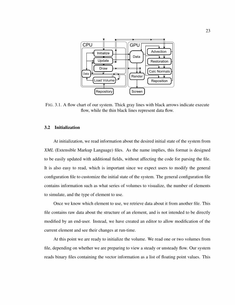
FIG. 3.1. A flow chart of our system. Thick gray lines with black arrows indicate executeflow, while the thin black lines represent data flow.

3.2 Initialization

At initialization, we read information about the desired initial state of the system from

XML (Extensible Markup Language) files. As the name implies, this format is designed

to be easily updated with additional fields, without affecting the code for parsing the file.

It is also easy to read, which is important since we expect users to modify the general

configuration file to customize the initial state of the system. The general configuration file

contains information such as what series of volumes to visualize, the number of elements

to simulate, and the type of element to use.

Once we know which element to use, we retrieve data about it from another file. This

file contains raw data about the structure of an element, and is not intended to be directly

modified by an end-user. Instead, we have created an editor to allow modification of the

current element and see their changes at run-time.

At this point we are ready to initialize the volume. We read one or two volumes from

file, depending on whether we are preparing to view a steady or unsteady flow. Our system

reads binary files containing the vector information as a list of floating point values. This

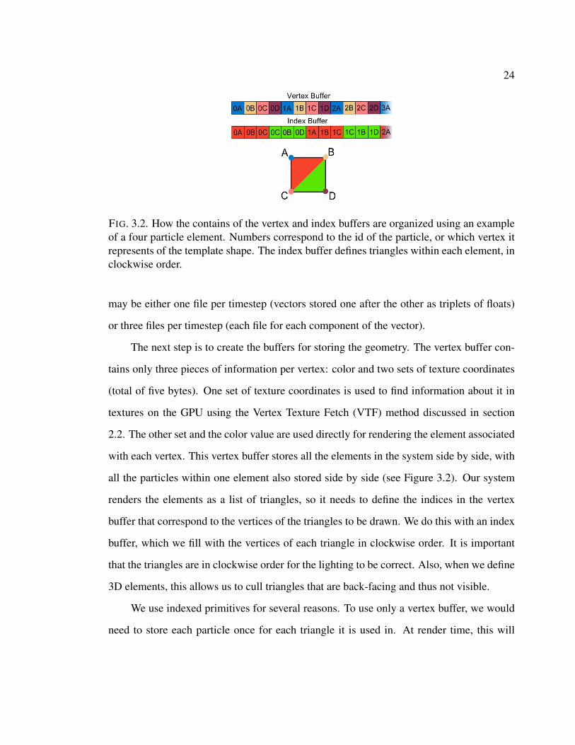
24

FIG. 3.2. How the contains of the vertex and index buffers are organized using an exampleof a four particle element. Numbers correspond to the id of the particle, or which vertex itrepresents of the template shape. The index buffer defines triangles within each element, inclockwise order.

may be either one file per timestep (vectors stored one after the other as triplets of floats)

or three files per timestep (each file for each component of the vector).

The next step is to create the buffers for storing the geometry. The vertex buffer con-

tains only three pieces of information per vertex: color and two sets of texture coordinates

(total of five bytes). One set of texture coordinates is used to find information about it in

textures on the GPU using the Vertex Texture Fetch (VTF) method discussed in section

2.2. The other set and the color value are used directly for rendering the element associated

with each vertex. This vertex buffer stores all the elements in the system side by side, with

all the particles within one element also stored side by side (see Figure 3.2). Our system

renders the elements as a list of triangles, so it needs to define the indices in the vertex

buffer that correspond to the vertices of the triangles to be drawn. We do this with an index

buffer, which we fill with the vertices of each triangle in clockwise order. It is important

that the triangles are in clockwise order for the lighting to be correct. Also, when we define

3D elements, this allows us to cull triangles that are back-facing and thus not visible.

We use indexed primitives for several reasons. To use only a vertex buffer, we would

need to store each particle once for each triangle it is used in. At render time, this will

25

require the vertex to be processed that number of times. With an index buffer, on graphics

hardware, the result of each index is stored in cache for a short time, so it can be reused for

repeat vertices (Pharr 1992). For our system, this may result in no repeated computation at

all, since the indices for each element are stored together, and the elements are sufficiently

small. Thus, although an index buffer only adds to the storage required (each vertex only

uses five bytes, whereas an index is stored using two bytes), saving redundant computation

should make rendering faster, especially for elements with a large number of triangles.

Furthermore, this method serves to separate the visual representation of an element from

the vertices, so if the user changes the triangles of the template element, we only need to

update the index buffer.

Elements are placed in the flow field at a random position inside a cube-shaped emit-

ter. The size of this emitter is specified in the configuration file. The elements are also

positioned using a random object frame, or a frame provided in the configuration file (see

Figure 3.3). This emitter can also be repositioned and resized at runtime using our interface.

We must also initialize the textures that will be used in our texture-based operations on

the GPU. These textures are the position texture, the normal texture, the reposition texture,

and the initial position texture. The position texture has one sample for each particle in

the system, and each sample only needs three channels in which it stores the position of

the particle. The normal texture computed on the GPU by rendering to this texture. All

other textures mentioned here will need to have duplicates, since we read the data for the

previous frame while writing data for the current frame.

3.3 Element Construction

Every element in the system is defined by a single template. The template defines the

number of particles in each element, a set of springs that will maintain the element’s shape,

26

FIG. 3.3. Elements are initialized in a cube emitter with a random (left) or a specified(right) object frame.

and a set of triangles that serve as its visual appearance. Figure 3.4 shows several examples

of the elements that can be defined with our method.

Notice that spring configuration can be independent of the apparent edges of the shape.

This is important, because it constitutes one of the most flexible features of our approach.

Defining different configurations will change how the element will retain its shape. For

instance, the cross shape on the lower left of Figure 3.4 defines springs between the out-

ermost points across the length of the shape, and between the corners of the cross. These

additional springs cause the cross to act more rigid, staying mostly flat. Remove them,

and the corners of the cross will fold in, and the shape will crumple up. This ability to

control not only the shape of the element, but degree of freedom in its deformation allows

for a wide variety of expression. We will discuss how we conduct the restoration process

in section 2.6.

Elements are instanced by using an object frame and a center position. Each particle

in the template is defined in world space with the origin as its center. Thus, we can apply

the object frame to the particles of the template and then add the center point to each result

to obtain world space coordinates for an instance of the element.

27

FIG. 3.4. Some example elements possible in our system. On the left is the spring configu-ration as it appears in the editor. On the right are the elements as they appear in simulation.

3.4 Particle Tracing

Particle tracing, or the advection of particles through the field, is done in a single

pass on the position data. For a single volume, we only need to apply equation 2.2, which

requires only one lookup into a 3D texture. However, we must consider how we sample

from the texture. Any given particle in the system is within some cell of the field, and thus

by point sampling the 3D texture we will retrieve the vector associated with that cell, which

would serve as the particle’s velocity until it moves into another cell. However, this may

result in sharp directional change as particles pass from one cell to another. Also, the fluid

flow that the volume represents would not have uniform blocks of steady direction, and

would instead change smoothly from position to position. Therefore, we must interpolate

between positions in the texture to provide a better approximation. We did this by setting

the texture sampler to linearly interpolate between cells.

When simulating advection through unsteady flows, we cannot abruptly switch from

the current volume to the next once that new volume as been transferred to the GPU. Since

this transfer will take time, the elements will advect in a single timestep for a second or

28

FIG. 3.5. The blue line plots the altitude at each depth in the volume, scaled between 0 and1. We approximate the inverse of this line so we can map the z coordinate to the correctaltitude in the volume stored linearly in the layers of a 3D texture (represented by the pinkline). The yellow line shows the result of applying our approximation to the layer altitudes,which follows the linearly increasing line closely.

more, spoiling the result. Also, it is equivalent to point sampling the fourth dimension of

the data, which will lead to sharp directional shifting. Instead, we apply linear interpolation

between the vector for timestep t and the vector from timestep t + 1 over an time interval.

This allows for a smooth transition between the timesteps. Once the time interval is over,

we should be able be ready to switch to the next volume in the sequence. We discuss this

process further in section 3.7.

In addition, we sometimes have datasets that need to be sampled in a non-linear man-

ner. For example, the wind speed data for Hurricane Bonnie was simulated at 27 altitudes,

and these values are plotted in Figure 3.5 on the blue line. To correctly map the z coordi-

nate of a particle to the linear storage of the volume, which follows the pink line, we need

to approximate the altitude curve with a function of x, and apply its inverse to z. The alti-

tudes increase polynomially, which we approximate with the curve defined by y = x1.8102.

We demonstrate this approximation by applying its inverse to the altitudes at each layer,

producing the yellow line in the figure. While the approximation is not perfect (does not

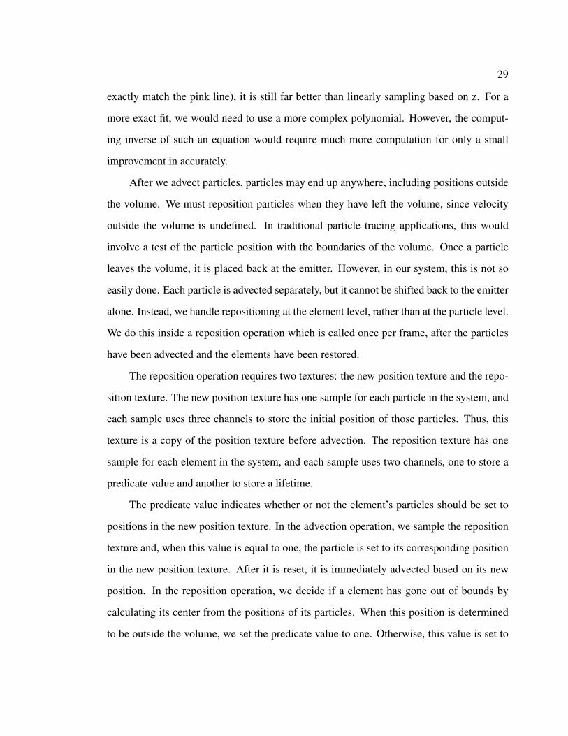
29

exactly match the pink line), it is still far better than linearly sampling based on z. For a

more exact fit, we would need to use a more complex polynomial. However, the comput-

ing inverse of such an equation would require much more computation for only a small

improvement in accurately.

After we advect particles, particles may end up anywhere, including positions outside

the volume. We must reposition particles when they have left the volume, since velocity

outside the volume is undefined. In traditional particle tracing applications, this would

involve a test of the particle position with the boundaries of the volume. Once a particle

leaves the volume, it is placed back at the emitter. However, in our system, this is not so

easily done. Each particle is advected separately, but it cannot be shifted back to the emitter

alone. Instead, we handle repositioning at the element level, rather than at the particle level.

We do this inside a reposition operation which is called once per frame, after the particles

have been advected and the elements have been restored.

The reposition operation requires two textures: the new position texture and the repo-

sition texture. The new position texture has one sample for each particle in the system, and

each sample uses three channels to store the initial position of those particles. Thus, this

texture is a copy of the position texture before advection. The reposition texture has one

sample for each element in the system, and each sample uses two channels, one to store a

predicate value and another to store a lifetime.

The predicate value indicates whether or not the element’s particles should be set to

positions in the new position texture. In the advection operation, we sample the reposition

texture and, when this value is equal to one, the particle is set to its corresponding position

in the new position texture. After it is reset, it is immediately advected based on its new

position. In the reposition operation, we decide if a element has gone out of bounds by

calculating its center from the positions of its particles. When this position is determined

to be outside the volume, we set the predicate value to one. Otherwise, this value is set to

30

zero, which assures that all other elements will not be reset, including ones that have just

been reset this timestep.

We also implement a lifecycle for the particles. After elements have been transported

within the same flow for a long time, they tend to become saturated, or trapped in some local

flow. To assure that the system of elements continues to reveal interesting features of the

entire field, we must reposition old particles back to their initial positions. This is done by

using the last channel of each reposition texture sample as the lifetime of each element. The

reposition operation decrements this value once per pass, and when an element’s lifetime

reaches zero, the element is repositioned. The lifetimes for the elements in the system

should be initialized to random values. If all the elements have the same lifetime, the entire

system of elements will be repositioned at once. This effect could be useful for viewing the

same advection into a flow several times, but generally is not desired.

Using this method, we reposition elements back to their initial starting position and

orientation. This should reveal information about change over time in unsteady flows, since

we will see the same element being advected differently when placed at various points in

time. However, in steady flows, this will result in the same exact element advection every

time. To solve this problem, we update the new position texture each frame with a random

set of particle positions. These random position allow us to see a much larger variety of

traces though the field.

3.5 Element Restoration

After the advection step, all of the particles have been moved slightly from their previ-

ous positions. Since our vector field may have vectors of any velocity per cell, it should be

assumed that the composite elements in the system are in slight disarray. In order to restore

the elements back to their original shape, we would need to solve a system of equations

31

corresponding to equation 2.6 for each spring in the element. Instead, we use a relaxation

scheme known as iteration which approximates the correct solution by solving for each

equation one at a time in sequence, and then repeating this process until the system con-

verges. In previous work, Jakobsen used Gauss-Seidel Iteration (Jakobsen 2001). In this

method, after each equation is solved, its new value immediately affects the next result.

Thus, the final result will depend on the order in which the equations are presented (Press

et al. 1992). Since we would like to have custom user-defined elements, we would rather

spring order not factor into the result.

An alterative is Jacobi Iteration, which differs from Gauss-Seidel in that it solves each

equation independently, and so they do not effect one another until the next iteration (Press

et al. 1992). This method converges at a much slower rate, but is not affected by the

sequence of the springs. In addition, Jacobi Iteration saves us the trouble of updating our

position texture after we update each spring in the system.

In actuality, we use a weaker version of Jacobi Iteration. In one pass over each particle,

we update based on all of its springs at once. To do this, we take the average of the forces

acting on the particle. This method will not converge as quickly, but we are not concerned

in this thesis about total convergence of the elements per frame. For applications in visual

effects, we would need to reconcile this inaccuracy and retain the illusion of rigid bodies

in the flow. For the purpose of visualization, deformed elements are actually a good visual

cue of strong local change.

To compute this step using a fragment program, we need a method for storing in-

formation about the springs on the GPU. We use a constant buffer with four component

vectors. These values correspond to the element IDs of the particles involved and the initial

length of the spring. This last component could be used to store a spring constant, but our

implementation restricts springs to infinite stiffness.

Each particle, based on its position in an element, must access some subset of this

32

spring buffer when it is processed in the restoration fragment program. The exact sub-

set used depends entirely on the spring configuration of the elements in the system. To

write a single fragment program to work for any configuration, we would need to use dy-

namic indexing within the fragment program. This feature is only available in DirectX 10

and requires additional instruction overhead (NVIDIA Corporation 2006). To avoid this

overhead, we decided to reconstruct our fragment program source whenever the element

template is changed. This run-time specialization of our shader code enables us to produce

fragment programs specifically for the spring structure of the current element.

3.5.1 Texture Layout

Over the course of our research we used two texture layouts for the particles. Origi-

nally, particle positions were mapped into a square texture exactly as the vertices appear in

the vertex buffer. This was changed to the current scheme which produces a strip of blocks

in order to improve the performance of the position and normal operations. Both of these

layouts are can be seen in Figure 3.6, and the following section discusses the disadvantages

of the square layout and how we improve performance by using a strip layout.

The first layout is inspired by the traditional method for storing particles on the GPU.

Previous approaches to GPU accelerated particle systems have used this method because,

by utilizing a OpenGL extension called Superbuffers, the position texture can double as a

vertex buffer by (Kipfer, Segal, & Westermann 2004; Kruger et al. 2005; Telea & van Wijk

2003). The problem with this method for our approach is two fold: First, this method hurts

the performance of the restoration and normal calculation operations. We use one fragment

program to apply the texture-based iteration scheme, which means that for each particle

in the system, there was one conditional in this program for that element. One problem

with this is that branching within a fragment program incurs large instruction overheads

(the equivalent of six instructions for each ”if else” statement on GeForce 6 series NVIDIA

33

FIG. 3.6. The texture layouts for example system of 16 elements with four particles each.The square layout was used first, and then we moved to a strip scheme with blocks ofidentical particles.

hardware) (Pharr 1992).

Another problem surfaces because of the layout of the texture. On graphics hardware,

when pixels are processed they are batched together in blocks. If every pixel inside of these

blocks executes the same control path, then only that path needs to be executed. However,

if some of these pixels branch differently, than all of the branches will need to be executed,

while only the results of the relative path are written. Notice in Figure 3.6 the example

of the layout for a four-particle element. While the IDs in the columns line up, every

consecutive pixel in each row represents a different vertex of an element, and thus will

take a separate control path. Therefore, there is no block of this texture that will take the

same path, and each program must compute the force for each spring in the element twice.

This is a substantial amount of wasted computation that grows with the complexity of the

element template.

Furthermore, this method requires one large fragment program, and these programs

take exponential time to compile based on instruction count with current DirectX com-

pilers. Each additional spring would require a noticeable increase in the compile time.

For example, compiling the shader code for a four-particle element with six springs would

34

compile in well under a minute, while an eight-particle element with 16 springs would take

roughly ten minutes.

Our solution was to use the strip layout, where texture is partitioned lengthwise into

blocks of particles with the same element ID. This would improve our performance on its

own, since processing the fragment program on one of these values will result in execution

of a single control path (except for border cases). However, now that we have blocks that

are uniform, we can get rid of the need for branching based on element ID by creating a

separate fragment program for each one. To update the particles, we render n rectangles

in a strip, where n is the number of particles per element. Each rectangles is sized and

positioned so that it rasterizes to the size of one of the blocks in the position texture, and

they are laid in a strip so that together they form one position texture when rendered. Now

we apply a different fragment program to each of these quads, one for each element id. Not

only do we avoid the overhead of branching, but since each of these programs is efficient

and small, our long compile times vastly improved, with the shader code for simulating all

of the element templates shown in Figure 3.4 taking seconds to compile.

3.6 Rendering and Surface Information

We have discussed how to advect particles and then restore them, but we have not yet

discussed how to render them. First, we need to calculate normals for all the particles in the

system so that their corresponding elements can be drawn. This is done in a GPU operation

acting on the position texture. For each particle in the system we add together the normal

of all the triangles the particle is a part of and normalize the result. This requires redundant

computation, which is one of the disadvantage of using a particle-centric scheme. Also,

given that every particle is a special case and the number triangles in the system are subject

to change, a triangle-centric approach is not feasible.

35

In section 3.2, we mentioned the vertex buffer and index buffer created at initializa-

tion. To position the triangles correctly in the scene, we use Vertex Texture Fetch to sample

the position texture and the normal at each vertex. This is done using special texture co-

ordinates stored at each vertex. We then use this information to position and shade the

element with simple Phong diffuse lighting. We also use color data and texture coordinates

stored at each vertex.

The color data constitutes the only reason we need to update the vertex buffer in

the update stage. We allow the user to reinitialize the particles during this stage, which

normally would not require updating the buffer. However, in order to help visualize the

mixing properties of the flow, we color elements based on the location of that element in

the flow. We use two schemes, layer coloring and radial coloring. Layer coloring involves

varying color based on location along some axis. Radial coloring depends on the distance

from the center on two axes. The type of color used is defined in the general configuration

file.

We can also color the surfaces based on the amount of average force being applied to

each particle. In this visualization, we use red to indicate a large amount of force acting on

a particle, and blue to indicate very little. Using this method, elements are shaded based

on the interpolation between the colors of their vertices, which serves as a good indication

of the vectors acting on each element locally. This is done by storing the average force

in the position texture at the restoration step. Then, the vertex shader that repositions the

geometry uses this value to determine the color.

Another method for the coloring the elements is lifetime. This involves sampling the

reposition texture in the vertex shader, choosing a color based on this value the same way

we did with the average force. This method enables a user to differentiate between elements

based on the amount of time they have been in the system.

In order to allow for generalized element structure, we cannot assume anything about

36

that structure. Moreover, since there are no duplicate vertices, we must use smooth shading,

finding the average of the triangles associated with each vertex, or particle. This causes 3D

elements to look blobby, which may not be the desired appearance. This can be seen clearly

in the screenshots of the cube, tetrahedron and partial Tu et al. fish (Tu & Termzopoulos

1994) elements shown in Figure 3.4. While this shading looks acceptable for the fish

element, geometry elements such as the cube and tetrahedron look strange. Still, our work

mostly focuses on 2D elements, so this is not a significant issue for our research.

3.7 Background Volume Streaming

In section 3.4, we discussed interpolating between two timesteps in order to produce

a smooth transition. This facilitates using unsteady flows, but we must have some way to

load volumes efficiently at run-time. Simply transferring an entire volume up to the GPU

at once will result in a momentary pause in the simulation, which is undesirable. We want

the simulation to animate as smoothly as possible. It is also not feasible to load all of

our timesteps onto the GPU at once. For instance, the Hurricane Bonnie dataset has 121

timesteps, each of which is 19.3 MB for a total of 2.3 GB. The GPU we used in our work,

a Geforce 7900 GTX, has only 512MB of on-GPU memory. Clearly, the CFD volumes

are the largest strain on memory in our system, thus we should minimize the number of

volumes stored concurrently in the system.

In order to do this, we store three volumes total on the GPU. Two loaded volumes are

used in the advection step, and a third set aside to load an additional volume. We use a

separate thread to page in new timesteps from file. When a volume is completely loaded,

we send it to the GPU one slice at a time. In this manner we distribute the loading over

multiple frames, which eases the burden on the bandwidth between the GPU and the CPU.

This results in a smaller drop in performance when transferring a volume.

37

Nevertheless, a problem arises when streaming these slices to the GPU. Since we are

not transferring a volume to the GPU when its still being loaded from file, there still a

noticeable difference in performance when using an uncapped frame rate. For this reason

we used a fixed time interval per frame, using the functionality provided by XNA Game

Studio (Microsoft 2007). This causes our largest possible frame-rate to be fixed at 60

frames per second, but the simulation appears much more uniform, which is essential to

our application. In the results chapter, we list the performance both with and without a

capped frame-rate.

Also, since our volume loading thread is not needed during the GPU transfer, it would

have to busy wait, or execute over the same loop until needed, which will be a strain on

CPU performance. To avoid this, we exit the thread after we load a volume, and spawn a

new thread each time a new volume is requested.

3.8 Application Interface

Since we endeavored to create a visualization which could be used by domain experts,

we wanted to allow easy customization of the simulation parameters. To achieve this, we

created two editors, one for managing volumes and another to allow the user to design and

modify molecules.

The volume editor allows the user to crop the volume series read from file (See Figure

3.7). If a volume has bad data on the outer edge, or if the user would like to focus on a

single feature in the volume, they may do so at run-time. The user selects the portion of

the volume that they want, and the rest is cropped away. From that point on, any volume

loaded into the system is also cropped to that size. In addition the editor allows users to

reposition the entire volume in relation to the camera and to reposition and resize the cube

emitter.

38

FIG. 3.7. Outlines that identify the bounds in the system. The blue bounds represents thebounds of the field, and the red bounds represents the field as it has been cropped by theuser, the yellow bounds are the bounds of the element emitter. The pink bounds representthe size of a single cell in the volume.

We also provide an element editor, which allows a user to modify anything about an

element, and the system makes the necessary changes when they leave the editor (after a

short pause, which can be up to several seconds). This editor also allows the user to save

the current version of the element for later use. Figure 3.4 shows what element templates

look like in the editor. The editor only allows for the creation of 2D elements, so to create

3D elements we made flat versions in the editor and then modified the z values in the

corresponding XML file.

Chapter 4

RESULTS AND EVALUATION

The following sections contain results from using our method. We provide perfor-

mance statistics on our systems performance, and discuss thoughts expressed by Lynn

Sparling, a domain expect on hurricane simulation and identification.

4.1 Performance

To measure the performance of our system, we used a machine with a dual core AMD

processor (4400+) with two GeForce 7900 GTX graphics cards and 2 GBs of RAM. While

there are two graphics cards, there is still only 512 MBs of video memory available, since

this memory is mirrored between the cards.

In Table 4.1, we have compiled the frame rates of our system when advecting elements

through one timestep of Hurricane Bonnie. These numbers were taken for separate runs

of the system with varying number of elements of varying complexity. The frame rate

is shown both using a fixed time interval (1/60 of a second) and variable time interval

per frame. The complexity values at the beginning of each row are shown in the format:

particles(triangles)[springs]. The frame-rate in each cell of the table is shown in the format:

fixed/variable. The last cell reads non-applicable (N/A) because we were not able to run

our system with this configuration. We discuss the cause of this limitation in section 4.3.

39

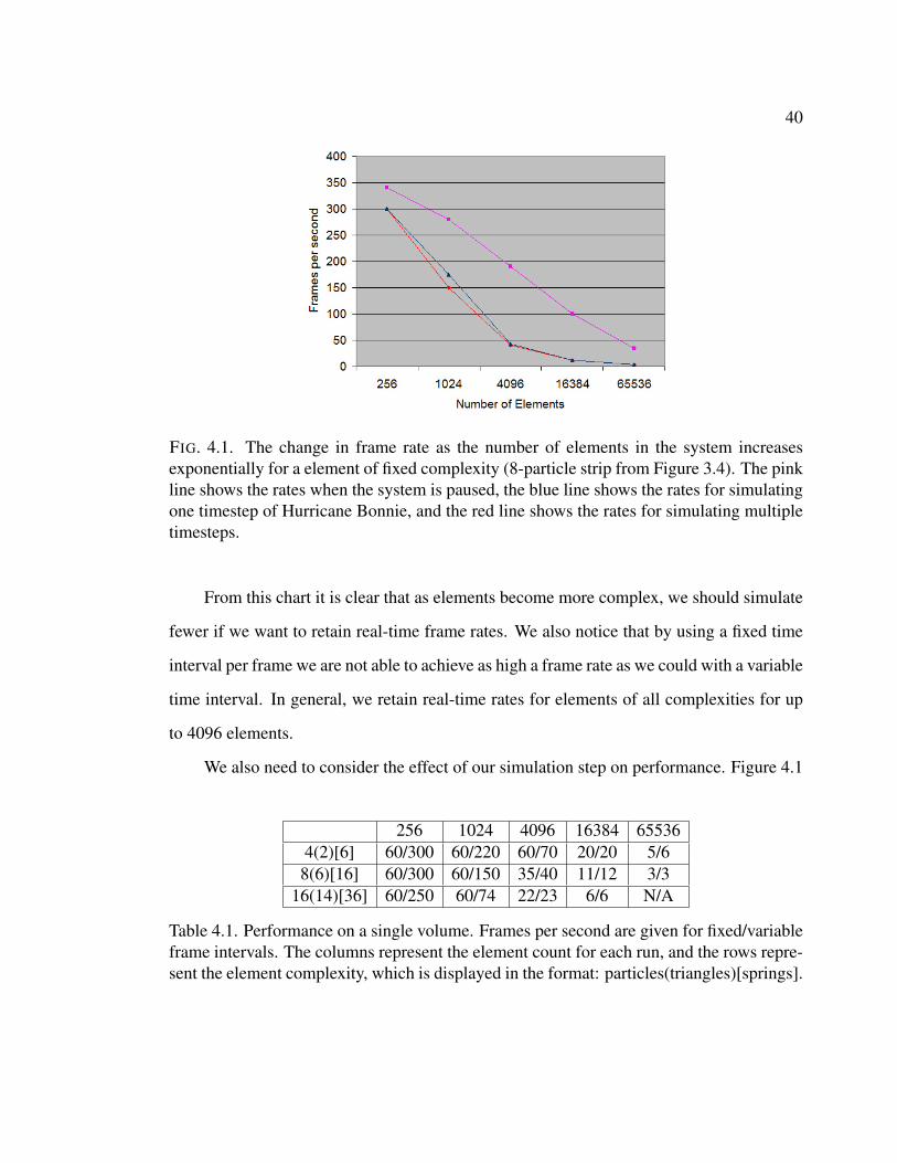
40

FIG. 4.1. The change in frame rate as the number of elements in the system increasesexponentially for a element of fixed complexity (8-particle strip from Figure 3.4). The pinkline shows the rates when the system is paused, the blue line shows the rates for simulatingone timestep of Hurricane Bonnie, and the red line shows the rates for simulating multipletimesteps.

From this chart it is clear that as elements become more complex, we should simulate

fewer if we want to retain real-time frame rates. We also notice that by using a fixed time

interval per frame we are not able to achieve as high a frame rate as we could with a variable

time interval. In general, we retain real-time rates for elements of all complexities for up

to 4096 elements.

We also need to consider the effect of our simulation step on performance. Figure 4.1

256 1024 4096 16384 655364(2)[6] 60/300 60/220 60/70 20/20 5/6

8(6)[16] 60/300 60/150 35/40 11/12 3/316(14)[36] 60/250 60/74 22/23 6/6 N/A

Table 4.1. Performance on a single volume. Frames per second are given for fixed/variableframe intervals. The columns represent the element count for each run, and the rows repre-sent the element complexity, which is displayed in the format: particles(triangles)[springs].

41

compares the performance of the system when paused (pink), when simulating a steady

flow (blue) and when simulating an unsteady flow (red). Notice that even with the system

paused, simply rendering the geometry using vertex textures becomes a strain on perfor-

mance as the element count increases. Also, the performance while paging in volumes is

very similar to the performance when simulating with one volume, which can be attributed

to our use of a separate thread to load volumes.

For unsteady flows, we would notice some marked slow down when paging in a new

volume to GPU. With a fixed time interval of 1/60 of a second, this dip is largely unnotice-

able (1-5 frames). However, when the time interval per frame is allowed to vary, we would

have large dips in frame rate (20-60). This would result in a noticeable change in the speed

of the elements in the system, where the elements slow down when paging in a volume and

speed up again when done. For this reason, the frame rates shown in Figure 4.1 by the red

line are the average frame-rate observed during the recorded runs.

4.2 Effectiveness

One of the features of flow that our system has been noticeably effective in demon-

strating is vorticity or local rotation within a flow (Rauber, Walsh, & Charlevoix 2005).

One cause of vorticity is wind shear, where the direction of the wind remains constant,

but the magnitude of the wind varies down an axis of the field. Singular particles would

move through such a field at different speeds, but would exhibit no vorticity. However, an

object moving through this field will rotate on its own axis based on the local change in

the magnitude along it. In their textbook on high impact meteorology, Rauder et al. use

paddlewheels to illustrate this trend, suspended in the flow particular to the wind direction

(Rauber, Walsh, & Charlevoix 2005). When the magnitude of the wind increases along the

paddlewheel, the wheel will move counterclockwise, and is said to have positive vortic-

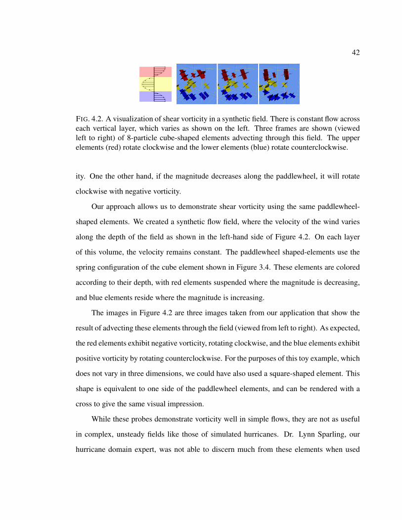
42

FIG. 4.2. A visualization of shear vorticity in a synthetic field. There is constant flow acrosseach vertical layer, which varies as shown on the left. Three frames are shown (viewedleft to right) of 8-particle cube-shaped elements advecting through this field. The upperelements (red) rotate clockwise and the lower elements (blue) rotate counterclockwise.

ity. One the other hand, if the magnitude decreases along the paddlewheel, it will rotate

clockwise with negative vorticity.

Our approach allows us to demonstrate shear vorticity using the same paddlewheel-

shaped elements. We created a synthetic flow field, where the velocity of the wind varies

along the depth of the field as shown in the left-hand side of Figure 4.2. On each layer

of this volume, the velocity remains constant. The paddlewheel shaped-elements use the

spring configuration of the cube element shown in Figure 3.4. These elements are colored

according to their depth, with red elements suspended where the magnitude is decreasing,

and blue elements reside where the magnitude is increasing.

The images in Figure 4.2 are three images taken from our application that show the

result of advecting these elements through the field (viewed from left to right). As expected,

the red elements exhibit negative vorticity, rotating clockwise, and the blue elements exhibit

positive vorticity by rotating counterclockwise. For the purposes of this toy example, which

does not vary in three dimensions, we could have also used a square-shaped element. This

shape is equivalent to one side of the paddlewheel elements, and can be rendered with a

cross to give the same visual impression.

While these probes demonstrate vorticity well in simple flows, they are not as useful

in complex, unsteady fields like those of simulated hurricanes. Dr. Lynn Sparling, our

hurricane domain expert, was not able to discern much from these elements when used

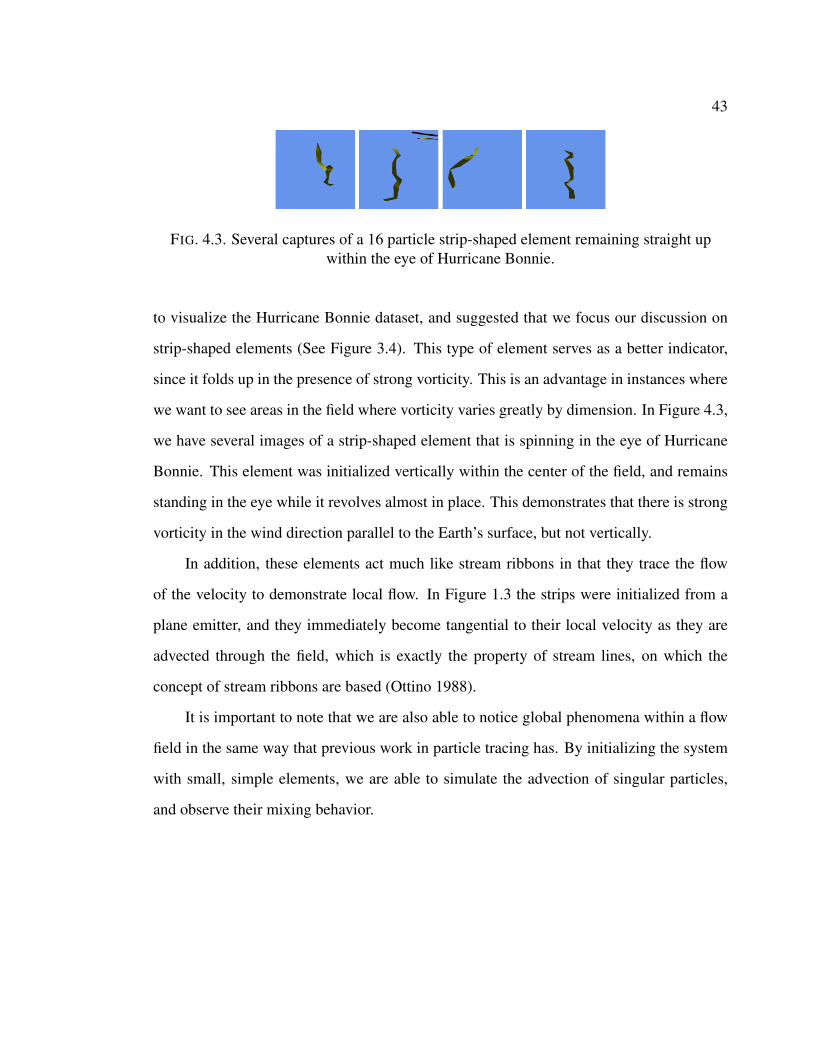
43

FIG. 4.3. Several captures of a 16 particle strip-shaped element remaining straight upwithin the eye of Hurricane Bonnie.

to visualize the Hurricane Bonnie dataset, and suggested that we focus our discussion on

strip-shaped elements (See Figure 3.4). This type of element serves as a better indicator,

since it folds up in the presence of strong vorticity. This is an advantage in instances where

we want to see areas in the field where vorticity varies greatly by dimension. In Figure 4.3,

we have several images of a strip-shaped element that is spinning in the eye of Hurricane

Bonnie. This element was initialized vertically within the center of the field, and remains

standing in the eye while it revolves almost in place. This demonstrates that there is strong

vorticity in the wind direction parallel to the Earth’s surface, but not vertically.

In addition, these elements act much like stream ribbons in that they trace the flow

of the velocity to demonstrate local flow. In Figure 1.3 the strips were initialized from a

plane emitter, and they immediately become tangential to their local velocity as they are

advected through the field, which is exactly the property of stream lines, on which the

concept of stream ribbons are based (Ottino 1988).

It is important to note that we are also able to notice global phenomena within a flow

field in the same way that previous work in particle tracing has. By initializing the system

with small, simple elements, we are able to simulate the advection of singular particles,

and observe their mixing behavior.

44

4.3 Limitations

We have observed several limitations to our approach. One such weakness is that in

order to clearly see the vorticity through element rotation, the application must be seen

in animation. While juxtaposed images taken over time are able to demonstrate simple

examples, the tumbling of elements in a complex field with three-dimensional variations

is must less apparent. It is much easier to recognize the rotation of the paddlewheels in

Figure 4.2 than it is to gauge the more complex motion of the strip in Figure 4.3. Since our

focus was on providing a highly interactive particle tracer, we concerned ourselves with

the real-time, dynamic portion of the application. We have left the addition of schemes for

portraying this motion in images to future work.

Particles are not repositioned unless their element center passes though the bounds.

This leads to particles that are outside the bounds of the volume, receiving incorrect treat-

ment in regards to advection. In Figure 4.4, we have several strip-shaped elements moving

through a synthetic field with a vertical shear. The strips should not deform, and simply ro-

tate until they are aligned with the velocity at some plane. While this motion is exhibited by

the elements overall, the portion of those elements on the boundaries are dragging behind.

This is a result of using the boundary velocity for extrapolation, since the shear disappears

for the portion of an element outside the volume. The only solution to this problem would

be to reposition an element once any one of its particles has goes out of bounds.

The current implementation is restricted to position textures whose dimensions must

be powers of two. This limits the number of elements in the system to some power of two.

This number must also be a perfect square, since the blocks within the position and normal

textures are square. The number of particles per elements must also be a power of two,

since this number determines the width of the textures. We have been able to demonstrate

our technique despite these limitations, but without them the system would be immensely

45

FIG. 4.4. Since an element are not replaced until its center is outside the bounds, particleswill drop outside the volume where velocity is not defined. These particles receive the samevelocity as the last layer, causing the outer portion of each element to appear to drag.

more flexible. To be able to include a given shape in our system, we must add or remove

vertices to its logical structure until we reach a power of two. For instance, we attempted

to recreate the fish skeleton described by Tu and Terzopoulos in their work on animating

artificial life (Tu & Termzopoulos 1994). However, the model uses 23 vertices, thus we

would need to increase its complexity by an additional 9 vertices. We created a truncated

version of the skeleton with 16 vertices, which can be seen upper right of Figure 3.4. The

original model had a tailfin and an additional point in the front. This happens again with the

cross-shaped element shown in the bottom left of Figure 3.4. Logically this shape should

only use 12 points, but we added 4 points in the center so that it would fit the requirement.

The strip texture layout limits the number of elements we can simulate at once. For

instance, we were not able to run our system for 65536 elements of 16 particles each, even

though this would require only 12 percent of the 512 MB available on our GPU. The reason

for this that the position and normal textures for these elements are 4096 by 256 and the

GPU is not able to find that much contiguous space in memory after reserving space for the

46

layers of three large volumes. The solution to this problem would be to size these textures

such that their dimensions are as equal as possible, but also so that they remain powers

of two. This would complicate indexing within the fragment programs, but the system

would make more efficient use of graphics memory, which would allow for the simulation

of larger numbers of elements and make it more reasonable to use this approach within

other applications for visual effect.

Chapter 5

CONCLUSION

5.1 Future Work

We have left a number of options open for extensions to our approach.

We observed when experimenting with our application that interesting things are pos-

sible when we allow springs to be defined between elements. Since every element is the

same, this would result in constraints across all elements, which would create a single

deformable structure. For example, by creating a spring between one element and the fol-

lowing element in the position texture in its row, we could create a ring of elements. At the

end of each row in the texture (or more accurately the texture block) we would move to the

start of the next row to find the next element in the sequence. Another possibility would be

to construct single particle elements with only external springs. Thus, every particle in the

system would have the same spring configuration, requiring only one square block rather

than a strip. By having springs defined in every direction we would create a complete lattice

of springs between all the particles in the system. Depending on how we wrap the texture

at boundaries, we can structure three different super sets with this configuration. If we ap-

ply no force over boundaries, we will simulate a sheet. If instead we wrap on boundaries,

connecting the beginning and end of all the rows and columns, we would create a donut. If

we wrap only rows or only columns, we would have a tube.

47

48

FIG. 5.1. An illustration of using a single particle spring configuration to simulate sheetelements like the one shown on the right. To the left is a position texture broken up intofour blocks. Each particle looks up in the eight positions around it in the texture, receivingforce from only those particles in its texture block.

While such global structures have some appeal, we can take this idea one step further.

We could divide the texture into blocks, and wrap on the boundaries of these block rather

than the boundaries of the entire texture. In this manner we can create several super sets at

once. For example, on the left side of Figure 5.1 we have simple position texture. To create

the sheet element on the right, we divide position texture into four blocks, and apply zero

forces at the block boundaries. This method would require only a single fragment program,

while we would need 16 separate programs using our method. Also, the block size could

be changed dynamically, without have to change the fragment program. The downside of

this method is that it would require looking up neighboring particles would require some

additional computation, which may result in a decrease in performance.

One valid extension would be to add additional surface information to the surface of

the elements. Since our elements are not single points in space, but objects, we can shade

their surfaces with color values that represent further information about their position. For

instance, we could provide a visual cue of a element direction or magnitude. We could also

calculate the vorticity the element is undergoing and display that.

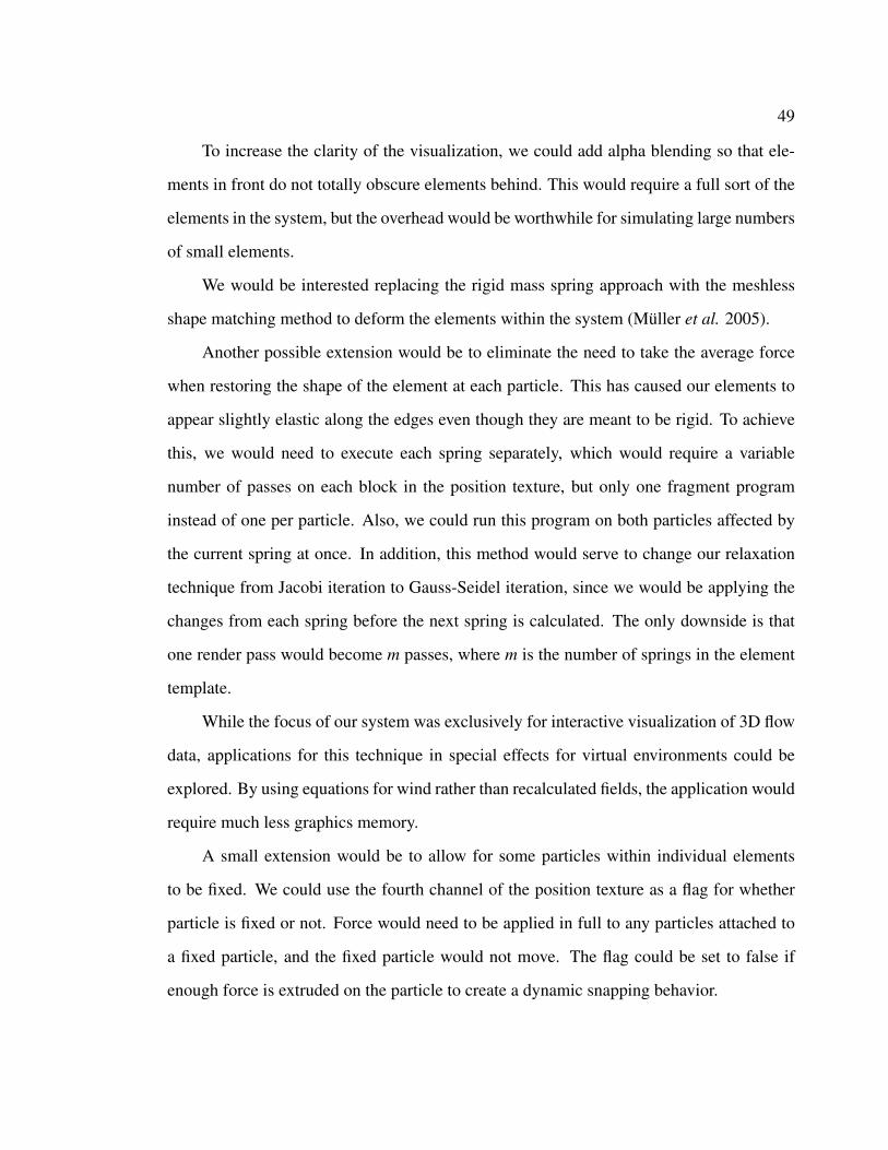
49

To increase the clarity of the visualization, we could add alpha blending so that ele-

ments in front do not totally obscure elements behind. This would require a full sort of the

elements in the system, but the overhead would be worthwhile for simulating large numbers

of small elements.

We would be interested replacing the rigid mass spring approach with the meshless

shape matching method to deform the elements within the system (Muller et al. 2005).

Another possible extension would be to eliminate the need to take the average force

when restoring the shape of the element at each particle. This has caused our elements to

appear slightly elastic along the edges even though they are meant to be rigid. To achieve

this, we would need to execute each spring separately, which would require a variable

number of passes on each block in the position texture, but only one fragment program

instead of one per particle. Also, we could run this program on both particles affected by

the current spring at once. In addition, this method would serve to change our relaxation

technique from Jacobi iteration to Gauss-Seidel iteration, since we would be applying the

changes from each spring before the next spring is calculated. The only downside is that

one render pass would become m passes, where m is the number of springs in the element

template.

While the focus of our system was exclusively for interactive visualization of 3D flow

data, applications for this technique in special effects for virtual environments could be

explored. By using equations for wind rather than recalculated fields, the application would

require much less graphics memory.

A small extension would be to allow for some particles within individual elements

to be fixed. We could use the fourth channel of the position texture as a flag for whether

particle is fixed or not. Force would need to be applied in full to any particles attached to

a fixed particle, and the fixed particle would not move. The flag could be set to false if

enough force is extruded on the particle to create a dynamic snapping behavior.

50

The only interactive interface features available are rotating the view, changing state,

or changing some system parameters such as element size and advection time interval. All

other interface features require the system to pause before they can take effect. It would

nice if the user could select a new position for the emitter in real-time.

Our system opens up some interesting avenues for experimentation with the different

perspectives available for fluid flow visualization. There are actually two ways to view

the velocity of a particle in a vector field (Ottino 1988). We have explored mainly the

Lagrangian viewpoint, which observes the motion of a particle through a field. The other

option is the Eulerian viewpoint, which observes the motion of particles at a certain posi-

tion. Our system is theoretically capable of providing observation from both viewpoints,

possibly simultaneously.

5.2 Conclusion

Vector field data is immense, so visualization methods that would display all of infor-

mation at once are impractical. In order to properly visualize this data, we must provide

some means of selective viewing it. We have demonstrated a graphics hardware accelerated

particle system with composite particle elements for the interactive visualization of vector

field data. This system is a variation on particle tracing, where single points in space are

transported through a field like dust in the wind. We create composite elements of these

particles by organizing them into sets that act according to an element template. This tem-

plate defines springs between particles that restrict their divergence, and triangles that serve

as their appearance. The elements are repositioned based on vector field data and restored

based on the average force acting on each particle along its springs. These operations are

done entirely in fragment programs on the GPU, allowing the system to transform a large

number of these dynamic shapes through a field at once. We are also able to simulate

51

unsteady flows by paging in volumes from file in a separate thread, and then transferring

them to the GPU one layer at a time. Using this method, we were able to visualize im-

portant aspects of simulated wind speed data for Hurricane Bonnie, such as vorticity and

stream lines. Our approach can be used to interactively visualize any series of vector fields,

and provides the same features as a traditional particle tracing system with the additional

benefit of observable vorticity using customizable probes.

REFERENCES

[1] Bruckschen, R. W.; Kuester, F.; Hamann, B.; and Joy, K. I. 2001. Real-time out-of-core

visualization of particle traces. In Breen, D.; Heirich, A.; and Koning, A., eds., IEEE

2001 Symposium on Parallel and Large-Data Visualization and Graphics (PVG2001),

45–50. Los Alamitos, California: IEEE.

[2] Chentanez, N. 2007. NVIDIA SDK white paper : Deformable bodies.

http://developer.download.nvidia.com/SDK/10/direct3d/samples.html.

[3] Georgii, J., and Westermann, R. 2005. Mass-spring systems on the GPU. Simulation

Modelling Practice and Theory 13:693–702.

[4] Guthe, S.; Gumhold, S.; and Strasser, W. 2002. Interactive visualization of volumetric

vector fields using texture based particles. Journal of WSCG 10:33–41.

[5] Haimes, R., and Darmofal, D. 1991. Visualization in computational fluid dynamics:

a case study. In VIS ’91: Proceedings of the 2nd conference on Visualization ’91, 392–

397. Los Alamitos, CA, USA: IEEE Computer Society Press.

[6] Hultquist, J. P. M. 1992. Constructing stream surfaces in steady 3d vector fields. In VIS

’92: Proceedings of the 3rd conference on Visualization ’92, 171–178. Los Alamitos,

CA, USA: IEEE Computer Society Press.

[7] Jakobsen, T. 2001. Advanced character physics - lecture. Game Developer’s Confer-

ence 2001.

[8] Jobard, B.; Erlebacher, G.; and Hussaini, M. Y. 2000. Hardware-accelerated texture

advection for unsteady flow visualization. In VIS ’00: Proceedings of the conference on

Visualization ’00, 155–162. Los Alamitos, CA, USA: IEEE Computer Society Press.

52

53

[9] Kipfer, P.; Segal, M.; and Westermann, R. 2004. Uberflow: a GPU-based particle

engine. In HWWS ’04: Proceedings of the ACM SIGGRAPH/EUROGRAPHICS confer-

ence on Graphics hardware, 115–122. New York, NY, USA: ACM Press.

[10] Kolb, A.; Latta, L.; and Rezk-Salama, C. 2004. Hardware-based simulation and

collision detection for large particle systems. In HWWS ’04: Proceedings of the ACM

SIGGRAPH/EUROGRAPHICS conference on Graphics hardware, 123–131. New York,

NY, USA: ACM Press.

[11] Kruger, J.; Kipfer, P.; Kondratieva, P.; and Westermann, R. 2005. A particle sys-

tem for interactive visualization of 3D flows. IEEE Trans. Visualization and Computer

Graphics 11(6):744–756.

[12] Latta, L. 2004. Building a million particle system. http://www.2ld.de/gdc2004.

[13] Microsoft. 2007. XNA game studio : XNA developer center at MSDN.

http://msdn2.microsoft.com/en-us/directx/aa937794.aspx.

[14] Muller, M.; Heidelberger, B.; Teshner, M.; and Gross, M. 2005. Meshless deforma-

tions based on shape matching. ACM Trans. Graph. 24(3):471–478.

[15] NVIDIA Corporation. 2006. Technical brief : NVIDIA geforce

8800 GPU architecture overview. Whitepaper, NVIDIA Corporation.

http://www.nvidia.com/page/8800 tech briefs.html.

[16] NVIDIA Corporation. 2007. NVIDIA CUDA compute unified de-

vice architecture : Programming guide. Whitepaper, NVIDIA Corporation.

http://developer.nvidia.com/object/cuda.html.

[17] Ottino, J. M. 1988. The kinematics of mixing: stretching, chaos, and transport.

Cambridge University Press.

54

[18] Owens, J. D.; Luebke, D.; Govindaraju, N.; Harris, M.; Krger, J.; Lefohn, A. E.; and

Purcell, T. J. 2005. A survey of general-purpose computation on graphics hardware. In

Eurographics 2005, State of the Art Reports, 21–51.

[19] Pharr, M., ed. 1992. GPU Gems 2: Programing Techniques for High-Performance

Graphics and General-Purpose Computation. Addison-Wesley Professional. chapter

The GeForce 6 Series GPU Architecture.

[20] Post, F. H., and van Walsum, T. 1993. Fluid flow visualization. In Focus on Scientific

Visualization, 1–40. London, UK: Springer-Verlag.

[21] Press, W. H.; Teukolsky, S. A.; Vetterling, W. T.; and Flannery, B. P. 1992. Numerical

Recipes in C. Cambridge University Press, second edition edition. chapter 19.5 Relax-

ation Methods for Boundary Value Problems. http://www.nrbook.com/a/bookcpdf.php.

[22] Rauber, R. M.; Walsh, J. E.; and Charlevoix, D. J. 2005. Severe & Hazardous

Weather: An Introduction to High Impact Meteorology. Kendall/Hunt Publishing Com-

pany, second edition edition.

[23] Reeves, W. T. 1983. Particle systems - a technique for modeling a class of fuzzy

objects. In SIGGRAPH ’83: Proceedings of the 10th annual conference on Computer

graphics and interactive techniques, 359–375. New York, NY, USA: ACM Press.

[24] Teitzel, C.; Grosso, R.; and Ertl, T. 1997. Efficient and reliable integration methods

for particle tracing in unsteady flows on discrete meshes. In Lefer, W., and Grave, M.,

eds., Eighth Eurographics Workshop on Visualization in Scientific Computing, 49–56.

[25] Telea, A., and van Wijk, J. J. 2003. 3D IBFV: Hardware-accelerated 3D flow vi-

sualization. In VIS ’03: Proceedings of the 14th IEEE Visualization 2003 (VIS’03),

233–240. Seattle, Washington, USA: IEEE Computer Society.

55

[26] Terzopoulos, D.; Platt, J.; Barr, A.; and Fleischer, K. 1987. Elastically deformable

models. In SIGGRAPH ’87: Proceedings of the 14th annual conference on Computer

graphics and interactive techniques, 205–214. New York, NY, USA: ACM Press.

[27] Tu, X., and Termzopoulos, D. 1994. Artifical fishes: phyics, locations, perception,

behavior. In SIGGRAPH ’94: Proceeding of the 21th annual conference on computer

graphics and interactive techniques, 43–50. New York, NY, USA: ACM.

[28] van Wijk, J. J. 1992. Rendering surface-particles. In VIS ’92: Proceedings of the

3rd conference on Visualization ’92, 54–61. Los Alamitos, CA, USA: IEEE Computer

Society Press.

[29] Verlet, L. 1967. Computer ”experiments” on classical fluids. i. thermodynamical

properties of lennard-jones molecules. Physical Review 159:98–103.

[30] Zeller, C. 2005. NVIDIA SDK white paper : Gpu cloth.

http://http.download.nvidia.com/developer/SDK/Individual Samples/3dgraphics samples.html.

[31] Zeller, C. 2007. NVIDIA SDK white paper : Cloth simulation.

http://developer.download.nvidia.com/SDK/10/direct3d/samples.html.