applying the technology of wireless sensor network in...

5

Applying the Technology of Wireless Sensor Network in Environment Monitoring

Constantin Volosencu “Politehnica” University of Timisoara

Romania

1. Introduction

This chapter presents some considerations related to the applications in environment

monitoring of some concepts as: estimation, fault detection and diagnosis, theory of

distributed parameter systems and artificial intelligence based on the modern technology of

wireless sensor networks. All these concepts allow treatment of large, complex, non-linear

and multivariable system of the environment by learning and extrapolation. The

environment may be seen as a complex ensemble of different distributed parameter systems,

described with partial differential equations.

Sensor networks (Akyildiz & all, 2002) have large and successful applications in monitoring

the environment, they been capable to measure, as a distributed sensor, the physical

variables, on a large area, which are characterizing the environment, and also to

communicate at long distance the measured values, from the distributed parameter

environmental processes. A lot of papers and books have been published in the fields of

using sensor networks in environment monitoring in the last years. Some related work is

surveyed as follows. The paper (Cuiyun & all., 2006) presents some research consideration

related the changes of urban spatial thermal environment, for sustainable urban

development, to improve the quality of human habitation environment. The urban thermal

phenomenon is revealed using thermal remote sensing imagery, based on the instantaneous

radiant temperature of the land surfaces. An architecture of sensor network for environment

is presented in (Lan & all, 2008). Environmental pollution and meteorological processes may

be studied using various kinds of environmental sensor networks. The modern intelligent

sensor networks comprise automatic sensor nodes and communication systems which

communicate their data to a sensor network server, where these data are integrated with

other environmental information. The paper (Giannopoulos & all, 2009) presents the design

and implementaion of a wireless sensor network for monitoring environmental variables

and evaluates its effectiveness. It has application in environment variable monitoring such

as: temperature, humidity, barometric pressure, soil moisture and ambient light, for

research in agriculture, habitat monitoring, weather monitoring and so on. In order to

improve the capacity of the environmental sensor networks different techniques may be

used. The paper (Talukder & all, 2008) is using a model predictive control for optimal

resource management in environment sensor networks, for with application at spatio-

temporal events of a coastal monitoring and forecast system. The paper (Dardari & all, 2007)

www.intechopen.com

Cutting Edge Research in New Technologies

98

presents and application at the estimation of atmospheric pressure using a wireless sensor

network, which is randomly distributes. The estimation error is dicussed and a design

criterion is proposed. The author has contribution in the field of monitoring distributed

parameter systems based on sensor networks and estimation using adaptive-network-based

fuzzy inference (Volosencu, 2010), (Volosencu & Curiac, 2010).

Using the modern intelligent wireless sensor networks multivariable estimation techniques may be applied in environment monitoring, seen as distributed parameter systems. Based on these concepts, environment monitoring becomes more easily and more performing (Fig. 1). The chapter presents a methodology of how to use the above mentioned topics in the problem of the environmental monitoring, as follows: - principles and technical data of modern sensor networks, - examples of distributed parameter systems, with their mathematical models, useful in environment description, - examples of modeling and simulation of environmental temperature variation, - technical data of the sensor network used in practical experiments, - a case study of environmental temperature estimation base on auto-regression and neuro-fuzzy inference engine.

Fig. 1. Scientific domains for environmental monitoring

The most important domains of applications are: the processes of heat conduction, with propagation of heat in anisotropy medium: propagation of heat in a porous medium, processes of transference of heat between a solid wall and a flow of hot gas; applications related to electricity domain as electrostatic charges in atmosphere; the motion of fluid, the processes of cooling and drying, phenomenon of diffusion. Other applications are: the growing of the gas particles in a fluid, the temperature modification in the air mass. The chapter presents a short survey of the main characteristics of the above topics involved in the problem of the environmental monitoring, some principles and technical data of modern sensor networks, some examples of distributed parameter systems, with their mathematical models, useful in environment description. The second paragraph presents some equation useful in modelling environmental processes. The third paragraph presents some estimation algorithms useful in environment monitoring, for future estimation of changing in physical variables of the medium. The fourth paragraph presents some examples of modelling and simulation of environmental temperature variation. The fifth paragraph presents some technical data of the sensor network used in practical experiments. The sixth paragraph presents the monitoring structure, the monitoring method and the estimation mechanism. The seventh paragraph presents an example of expert system useful in environment monitoring, based on environment knowledge. The eighth paragraph presents a case study. The ninth paragraph presents a technical solution of implementation

www.intechopen.com


99

of the monitoring system based on virtual instrumentation. The main results and future perspectives are presented in conclusion.

2. Equations for environmental systems

2.1 Primary physical and mathematical models

The environment systems, which are complex heterogeneous systems of distributed

parameter systems, may be described using partial differential equations. These equations

are used to formulate problems involving functions of several variables, such as the

propagation of sound or heat, electrostatics, electrodynamics, fluid flow. Some examples of

distributed parameter systems are presented as follow (Rosculet & Craiu, 1979). Diverse

categories of systems have specific characteristics that are important in their investigation,

simulation, prediction, monitoring and diagnosis. One of the most important domains of

applications is represented by the process of heat conduction, with propagation of heat in

anisotropy medium. In the field of motion of fluid there are: plane motion of viscous fluids,

running of viscous fluids in medium as a tube or running of gases. The processes of cooling

and drying are also met in environment systems. Phenomenons of diffusion could be:

diffusion flow for chemical reactions, the flames diffusion, the density repartition of

particles loading by the meteorites. Other applications in the environment could be:

estimation of the ice height covering the snow the arctic seas, motion of underground

waters, the growing of the gas particles in a fluid, the temperature modification in the air

mass. For some of the above processes some equations are given as follows.

The function of the object’s temperature is (P, t), at the time moment t, where P is a point in

the space. If different points of object have different temperatures, (P, t)ct., then a heat

transfer will take place, from the warmer parts to the less warm parts. The vector grad has

its direction along the normal at the level surface for =ct., in the sense of rising. The law of heat propagation through an object in which there are no heat sources:

k k kt x x y y z z

(1)

The heat sources in the object have a distribution given by the function:

( , ) ( , , , )F t P F t x y z (2)

If the object is homogenous / / .a k ct and the equation (2) is written:

2

1

t x x y y z za

(3)

The initial conditions or of the limit conditions have physical significance. They are given by the equation:

0

( , , , ) ( , , )t

x y z t f x y z (4)

Running of viscous fluids in rectilinear medium may be analyzed with he following equations. Let it be a rectilinear medium, which is leading a viscous liquid. The ax of

www.intechopen.com


100

medium, seen as a tube is Oz. Let us consider the movement of a part of the liquid between two transversal sections z1 and z1+h. If A is the transversal section area supposed to be

constant and is the fluid density, the movement equation is

1 2( )v

Ah A p p Rt

(5)

where p1 and p2 are the pressures in the two sections and R is the force on the tube wall. If v is

the fluid speed in the direction of Oz axis, v is independent of z if the liquid is incompressible

( , , )v v x y t (6)

The partial derivative equation is

2 2

2 2

pv v v

t z x y (7)

if the pressure p is constant

2 2

2 2

1 v v v

a t x y

(8)

which it is the equation of heat propagation in plane, where a=/. For the plane motion of viscous fluids let’s consider an incompressible, viscous fluid of

constant density , in a plane movement. If (vx, vy) are the speed components in the point

P(x, y) of the plane at the time moment t , the movement equations are

1

1

x x xx y x

y y yx y y

pv v vv v v

t x y x

v v v pv v v

t x y y

(9)

where p is the pressure in this point, , is the viscosity coefficient. At the equations (5)

the equations of continuity are added

0yx

vv

x y

(10)

The current function is introduced

x

vy

v yx

, (11)

Analyze of the no stationary heat in subterranean could be done when a series of problems

arise at the calculation of heat losses in conditions of a heat change no stationary. For

determining the no stationary heat losses in the subterranean, the next equation is used

www.intechopen.com


101

2 2

2 2s sa

t x y

(12)

where is the temperature of the material, s is the soil temperature, t is the time, x, y are the Cartesians coordinates and a is a coefficient what is characterizing soil thermal diffusion. Suddenly in practice a great importance is to analyze the running of gases, to establish the pressure in a certainly point of a medium. The no stationary running of a gas is defined by the system

2

2

p v v

x t d

v

t x

(13)

where p is the pressure, v is the speed related at a section, d is the medium diameter and is the friction coefficient. A method used to determine the ice height of the arctic seas is the radiometry. Radiometry is based on registration of the heat radiation of which intensity varies with temperature and the radiation coefficient of the objects. The value of the radiations will characterize the relation between ice heights in their different stages. The temperature of the ice surface is determined from the heat equation, which describes the heat repartition in snow and ice

2

2, 1,2,3

jj j jc j

t z

(14)

where cj is the specific heat, j is the density, j is the thermal conductivity coefficient, j is the temperature, t is the time, z is the height coordinate. The indices j=1,2,3 correspond to the there medium: air, snow and ice. At the frontiers there are the conditions of equilibrium.

2.2 General equations for modeling environment system seen as distributed parameter systems The distributed parameter systems have general mathematical models in continuous time and space as partial differential equation, of parabolic or hyperbolic form, as:

1 2 3( )c c c Qt

(15)

2

1 2 32( )c c c Q

t

(16)

where the variables (, t) are depending on time t0 and on space V, where is x for one axis, (x, y) for two axis or (x, y, z) for three axis, c1, c2 and c3 are coefficients, which could be also time variant and Q(, t) is an exterior excitation, variable on time and space. So, in the general case, an implicit equation may be written:

22

2 2, . , ,... 0f

t t

(17)

www.intechopen.com


102

For the partial differential equations (1, 2) some boundary conditions may be imposed to

establish a solution. So, when the variable value of the boundary is specified, there are

Dirichlet conditions:

4c q (18)

And, when the variable flux and transfer coefficient are specified, there are Neumann

conditions:

5 6 0c c (19)

In the practical application case studies limits and initial conditions of the equation (1) are

imposed:

0(0, ) , [0, ], ( ,0) 0, [0, ],

( , ) , [0, ]l

t t T l

l t t T

(20)

A system with finite differences may be associated to the equations (1) and (2). For this

purpose the space S is divided into small dimension pieces lp:

/pl l n (21)

In each small piece Spi, i=1,…,n of the space S the variable could be measured at each

moment tk, using a sensor from the sensor network, in a characteristic point Pi(i), of

coordinate i. Let it be ik the variable value in the point Pi(i) at the moment tk.

The points from the space in which the phenomenon is happening are denoted Pi, with the

coordinate zi. For a bi-dimensional space in a system coordinate xOy zi=(xi,yi). The

phenomenon as distributed system is monitored with a sensor network with n sensors Si,

i=1,…,n, placed in n points Pi from the space, like in Fig. 2.

Fig. 2. Space monitoring scheme

It is a general known method to approximate the derivatives of a variable with small

variations. In the equation with partial derivatives there are derivatives of first order, in time,

and derivatives of first and second order in space. So, theoretically, we may approximate the

variable derivatives in time with small variations in time, with the following relations:

www.intechopen.com


103

-

-

1

1

k ki i

k kt t t

(22)

2 - 21 1

2 21( )

k k ki i i

k kt t t

(23)

The first and the second derivatives in space may be approximated with small variations

in space to obtain the following relations. For the x-axis we may write the following

equations:

-- 1k ki i

px l

(24)

2 - 21 1

2 2

k k ki i i

px l

(25)

The same equations may be written also for the y and also z-axis. Of course, an equation

with variables written in vectors could be written.

We may consider the variable is measured as the sample ),( kiki t , iV, at equal time

intervals with the value:

-1k kh t t (26)

called sample period, in a sampling procedure, with a digital equipment, at the sample time

moments tk=k.h.

For the above equation, a linear approximate system of derivative equations of first degree

may be used:

d

A BQdt

(27)

where, this time, is a vector containing the values of the variable (, t) in different points

of the space and at different time moments.

Combining the equations (17, 22, 24) in equation (15), a system of equations with differences results for the parabolic equation:

-1

1 1( , , , ) 0k k k kp i i i if (28)

and, combining the equations (17, 23, 25) in equation (16), an equivalent system with differences results as a model for the hyperbolic equation:

- - -1 1 1

1 1 1 1( , , , , , ) 0k k k k k kh i i i i i if (29)

Taking account of equations (28, 29), it is obvious that several estimation algorithms may be

developed as follows, based on the discrete models of the partial derivative equations. These

algorithms of estimation are presented as it follows.

www.intechopen.com


104

3. Algorithms of estimation

3.1 Parabolic systems

Estimation algorithm 1. It estimates the value of the variable 1ki at the moment tk+1,

measuring the values of the variables -1 1, ,k k ki i i at the anterior moment tk:

( )ki

ki

ki

ki f θ,θ,θ=θ +-

+111

1 (30)

This is a multivariable estimation algorithm, based on the adjacent nodes.


measuring the values of the same variable - - -1 2 3, , ,k k k ki i i i , but at four anterior moments tk,

tk-1, tk-2 and tk-3.

- - -1 1 2 32 , , ,k k k k k

i i i i if (31)

This is an autoregressive algorithm, using the values from the same node.

3.2 Hyperbolic systems


measuring the values of the variables -1 1, ,k k ki i i at the anterior time moment tk and tk-1:

( )111

11111

1 __

+

_

-+-+ θ,θ,θ,θ,θ,θ=θ k

iki

ki

ki

ki

ki

ki f (32)

This is a multivariable estimation algorithm, based on the adjacent nodes and 2 time anterior moments.


measuring the values of the same variable (the same node) - - - - -1 2 3 4 5, , , , ,k k k k k ki i i i i i , but at

six anterior moments tk, tk-1, tk-2, tk-3, tk-4and tk-3:

( )543212

1 -----+ θ,θ,θ,θ,θ,θ=θ ki

ki

ki

ki

ki

ki

ki f (33)

4. Modeling and simulation

Environment behavior may be modeled with the equation from the above paragraph. Using these models, some analysis in time and space domains may be accomplished. Some transient characteristics of the temperature are there presented for 101 samples. The nodes and meshes structure for a sensor network with reduced number of sensor, in this case 13, is presented in Fig. 3.

Fig. 3. Nodes and meshes for heat transfer in plane

www.intechopen.com


105

The temperature variation in 3D is presented in Fig. 4, at a certain time moment.

Fig. 4. Temperature variation in space

Temperature isotherms in plane are presented in Fig. 5.

Identical characteristics may be obtained for other distributed parameter systems involved

in environmental modeling.

Fig. 5. Temperature isotherms

5. Sensor network

The modern sensors are smart, small, lightweight and portable devices, with a

communication infrastructure intended to monitor and record specific parameters like

temperature, humidity, pressure, wind direction and speed, illumination intensity, vibration

intensity, sound intensity, power-line voltage, chemical concentrations and pollutant levels

at diverse locations. The sensor number in a network is over hundreds or thousands of ad

hoc tiny sensor nodes spread across different area. Thus, the network actively participates in

creating a smart environment. With them we may developed low cost wireless platforms,

including integrated radio and microprocessors. The sensors are adequate for autonomous

operation in highly dynamic environments as distributed parameter systems. We may add

sensors when they fail. They require distributed computation and communication protocols.

They insure scalability, where the quality can be traded for system lifetime. They insure

Internet connections via satellite.

The structure of a modern sensor is presented in Fig. 6.

www.intechopen.com


106

Fig. 6. The structure of a modern sensor

The constructive and functional representation of a sensor network is presented in Fig. 7.

Fig. 7. Sensor network

The sensor SA measures the temperature A in a point in this space. The sensor SA measures the temperature A in a point in this space. There have been used in practice: a Memsic eKo Outdoor Wireless Monitoring System with 4 eKo sensor nodes EN2100, an eKo base radio EB2110, an eKo gateway w/ built-in eKoView web application. The eKo Wireless Sensor Nodes form wireless mesh network with communication range from several hundred meters, accepting up to four sensor inputs. Solar cell or rechargeable batteries powered them. The eKo base radio provides connection between eKo sensor nodes and eKo gateway via USB interface for data transfer. pThere had been used an eKo weather station sensor suite with wind speed, wind direction, rain gauge, ambient temp/humidity, barometric pressure and solar radiation. Each node has a temperature and humidity sensor to measure the ambient relative humidity and air temperature and to calculate the dew point. The base station is wireless, with computing energy and communication resources, which is acting like an access gate between the sensor nodes and the end user. The senor nodes have two components. The processor/radio modules are activating the measuring system of small power.

Fig. 8. Components of the sensor network used in practice

www.intechopen.com


107

They are working at the frequency of 2.4 GHz. The sensor network is also provided with a software for data acquisition, which is reading data from a data base. The sensor network is working in real time with a driver which insures data acquisition from the base station.

6. Monitoring application

6.1 Monitoring structure

The estimation model describes the evolution of a variable measured over the same sample period as a non-linear function of past evolutions. This kind of systems evolves due to its “non-linear memory", generating internal dynamics. The estimation model definition is:

1( ) ( ( ),..., ( ))ny t f u t u t (34)

where u(t) is a vector of the series under investigation (in our case is the series of values measured by the sensors from the network):

1 2 ...T

nu u u u (35)

and f is the non-linear estimation function of non-linear regression, n is the order of the regression. By convention all the components u1(t),…,un(t) of the multivariable time series u(t) are assumed to be zero mean. The function f may be estimated in case that the time series u(t), u(t-1),…, u(t-n) is known (recursive parameter estimation), either predict future value in case that the function f and past values u(t-1),…, u(t-n) are known (AR prediction). The method uses the time series of measured data provided by each sensor and relies on an (auto)-regressive multivariable predictor placed in base stations as it is presented in Fig. 9.

Fig. 9. Estimation and detection structure

The principle of the estimation is: the sensor nodes will be identified by comparing their

output values (t) with the values y(t) predicted using past/present values provided by the same sensors or adjacent sensors (adj). After this initialization, at every instant time t the

estimated values are computed relying only on past values A(t-1), …, A(0) and both parameter estimation and prediction are used. First, the parameters of the function f are estimated using training from measured values with a training algorithm as back-

propagation, for example. After that, the present values ( )A t measured by the sensor

nodes may be compared with their estimated values y(t) by computing the errors:

-( ) ( ) ( )A Ae t t y t (36)

www.intechopen.com


108

If these errors are higher than the thresholds A at the sensor measuring point, a fault occurs.

Here, based on a database containing the known models, on a knowledge-based system, we

may see the case as a multi-agent system, which can do critics, learning and changes, taking

decision based on node analysis from network topology. Two parameters can influence the

decision: the type of the distributed parameter system, which is offering the data measured by

sensors and the computing limitations. Because both of them are a priori known, an off-line

methodology is proposed. Realistic values are situated between 3 and 6.

6.2 Estimator mechanism

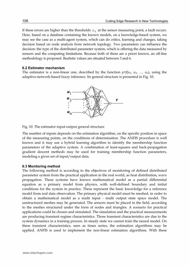
The estimator is a non-linear one, described by the function y=f(u1, u2, …, un), using the

adaptive-network-based fuzzy inference. Its general structure is presented in Fig. 10.

Fig. 10. The estimator input-output general structure

The number of inputs depends on the estimation algorithm, on the specific position in space

of the measuring points, on the conditions of determination. The ANFIS procedure is well

known and it may use a hybrid learning algorithm to identify the membership function

parameters of the adaptive system. A combination of least-squares and back-propagation

gradient descent methods may be used for training membership function parameters,

modeling a given set of input/output data.

6.3 Monitoring method

The following method is according to the objectives of monitoring of defined distributed

parameter system from the practical application in the real world, as heat distribution, wave

propagation. These systems have known mathematical model as a partial differential

equation as a primary model from physics, with well-defined boundary and initial

conditions for the system in practice. These represent the basic knowledge for a reference

model from real data observation. The primary physical model must be meshed, in order to

obtain a mathematical model as a multi input - multi output state space model. The

unstructured meshes may be generated. The sensors must be placed in the field, according

to the meshes structured under the form of nodes and triangles. A scenario for practical

applications could be chosen and simulated. The simulation and the practical measurements

are producing transient regime characteristics. Those transient characteristics are due to the

system dynamics in a training process. In steady state we cannot train the neural model. On

these transient characteristics, seen as times series, the estimation algorithms may be

applied. ANFIS is used to implement the non-linear estimation algorithms. With these

www.intechopen.com


109

algorithms, future states of the process may be estimated. Possible fault in the system are

chosen and strategies for detection may be developed, to identify and to diagnose them,

based on the state estimation. In practice, applying the method presumes the following

steps: -placing a sensor network in the field of the distributed parameter system; -

acquiring data, in time, from the sensor nodes, for the system variables; -using measured

data to determine an estimation model based on ANFIS; -using measured data to estimate

the future values of the system variables; -imposing an error threshold for the system

variables; -comparing the measured data with the estimated values; -if the determined

error is greater then the threshold, a default occurs; -diagnosing the default, based on

estimated data, determining its place in the sensor network and in the distribute

parameter system field.

7. Expert system

7.1 Process knowledge

Knowledge that may be determinate from measurements upon the process variables made

using sensor networks is as it follows:

- the value vi of the phenomenon at a time moment, in a point of the space Pi, which is

the value provided by the sensor Si, place in the point Pi, at the time moment t: i(t),

temperature in this case;

- the speed of the phenomenon si, which is the derivative in time of the variables measured by sensor Si, in the point Pi, at two consecutive time moments t and t-h:

- -( ) ( ) ( )i i id t t t h

dt h

, where the discrete time approximation is used, for a constant

sample period h;

- the value of the difference in space dij, from two adjacent sensor variables: ij(t) = i(t)- j(t), given by the sensors Si and Sj, place din the points Pi and Pj; -the difference in space

is given the sense in which the phenomenon is happening. The positive sense is

considering from Si to Sj. This difference is proportional to the space between two

sensors Si to Sj, or points Pi and Pj lij=|zi-zj|, where zi and zj are the space coordinates of

the two points. For a bi-dimensional space, the coordinates are for Pi(xi,yi) and Pj(xi, xj).

- the speed sdij of difference variation between two adjacent sensors Si and Sj, place din

the points Pi and Pj, as time derivative of space difference - -( ) ( ) ( )ij ij ijd t t t h

dt h

,

at two onsecutive time moments t and t-h. The speed of the difference in space is given

the speed of the space displacement in a sense in which the phenomenon is happening.

We may use also the variables obtained as estimation, as it follows.

- the estimated value ^

iv of the phenomenon at a time moment, in a point of the space Pi,

which is the value provided by the estimator Ei for the point Pi, at the time moment t: ^

( )i t ;

- the speed of the estimated phenomenon is^

, which is the derivative in time of the

estimated variables provided by the estimator Ei for the point Pi, at two consecutive

www.intechopen.com


110

time moments t and t-h: h

htt

dt

td iii )-(-)()(^^^

, where the discrete time approximation

is used, for a constant sample period h;

the estimated difference in space ^

ijd , from two values of two adjacent sensor variables:

^

-^ ^

( ) ( ) ( )ij i jt t t , given by the estimators Ei and Ej, for the points Pi and Pj; The estimated

difference in space is given the estimated sense in which the phenomenon is estimated to

take place.

- the estimated speed ^

ijsd of the estimated difference variation between two estimators Ei

and Ej, for two adjacent points Pi and Pj, as time derivative of estimated space difference ^

- -^ ^

( ) ( ) ( )ij ij ijd t t t h

dt h

, at two consecutive time moments t and t-h. The speed of

the difference of estimates in space is given the speed of the estimate of the space

displacement in a sense in which the phenomenon is estimated to happen.

Some errors between the estimates and the actual variables may be introduced: -^

ve v v -

the error at the process value; -^

se s s - the error in speed of phenomenon happening in

some field point; -^

de d d -the error in space difference of two adjacent points and

-^

sde sd sd - the error of speed of phenomenon propagation in space.

In order to make estimations, we may use the values provided by the sensors.

7.2 Expert system structure

For these process variables v, s, d, sd and for the estimated variables ^ ^ ^ ^

, , ,v s d sd some values

may be defined as negative N and positive P or around zero Z, with some degrees: small S, medium M or big B. So, we may have the following combinations put on an axis: NB, NM,

NS, Z, PS, PM, PB. To emphasize a non-linear character of the process, the usage of only three fuzzy values is recommended. The reasoning is as it follows: -If the derivatives are negative, we may say the phenomenon

is decreasing. -If the derivative are positive, the phenomenon is increasing; -If the differences are negative, the phenomenon sense is opposite from the two sensors and measuring points. - If the speed of the difference is positive, the space becomes to be not homogenous, something is happening in the space between the two sensors.

The expert system is developed using a backward chaining. Some rules from the rule base for this expert system are: (1) IF v is Z THEN the process is supressed (cf = 10 %); (2) IF v is NOT Z THEN the process is NOT supressed (cf = 90 %); (3) IF s is Z THEN the process is

NOT in course (cf = 10 %); (4) IF s is NOT Z THEN the process is in course (cf = 90 %), and so on. Many other rules may be developed according to the above considerations. The application may be framed in so called “goal driven methods”. In the real distributed parameter systems there are phenomena with small certainty and their opposite seems to be

www.intechopen.com


111

true. When an exert system is developed for monitoring distributed parameter systems, it is necessary to test both, to see what it is happening in the field.

8. Case study

There is presented a basic case study consisting in a heat distribution flux through a plane square surface of dimensions l=1, with Dirichlet boundary conditions as constant temperature on three margins:

h r (37)

with r=0, and a Neumann boundary condition as a flux temperature from a source

nk q g (38)

where q is the heat transfer coefficient q=0, g=0, h=1. The heat equation, of a parabolic type, is:

( ) ( )extC k Q ht

(39)

where is the density of the medium, C is the thermal (heat) capacity, k is the thermal

conductivity, coefficient of heat conduction, Q is the heat source, h is the convective heat

transfer coefficient, ext is the external temperature. Relative values are chosen for the

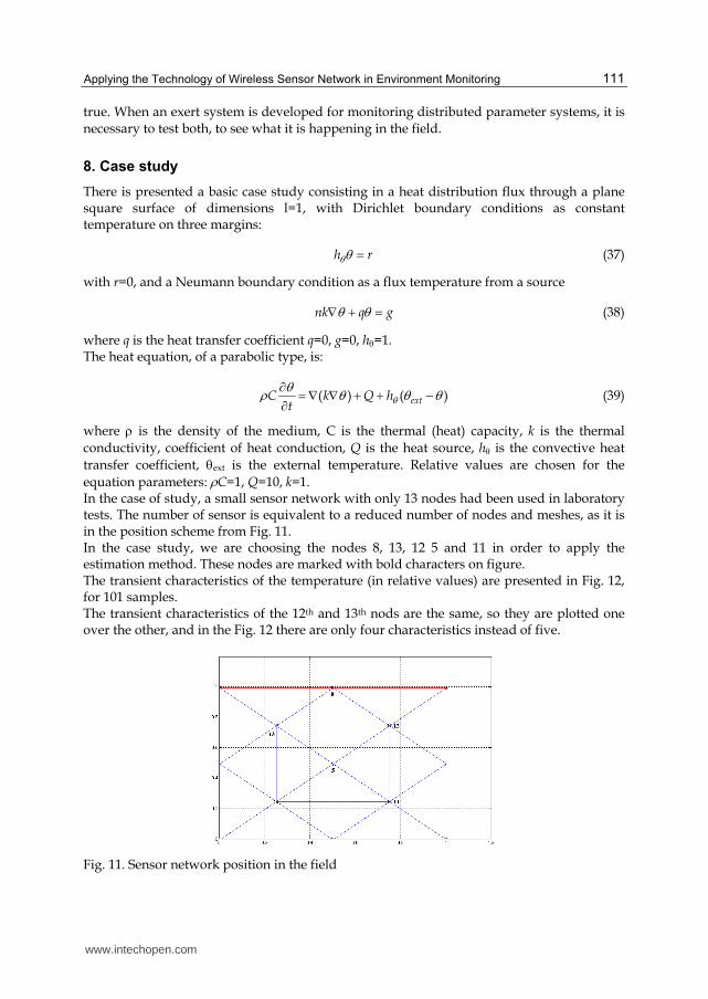
equation parameters: C=1, Q=10, k=1. In the case of study, a small sensor network with only 13 nodes had been used in laboratory tests. The number of sensor is equivalent to a reduced number of nodes and meshes, as it is in the position scheme from Fig. 11. In the case study, we are choosing the nodes 8, 13, 12 5 and 11 in order to apply the estimation method. These nodes are marked with bold characters on figure. The transient characteristics of the temperature (in relative values) are presented in Fig. 12, for 101 samples. The transient characteristics of the 12th and 13th nods are the same, so they are plotted one over the other, and in the Fig. 12 there are only four characteristics instead of five.

Fig. 11. Sensor network position in the field

www.intechopen.com


112

Fig. 12. Transient characteristics

We are presenting as an example the estimation for the 5th node. It is the node of the estimated variable, based on the first recursive algorithm:

15 8 13 12 11( , , , )k k k k kf (40)

The fuzzy inference system structure is presented in Fig. 13.

Fig. 13. FIS structure

A short description about the ANFIS and its function approximating property is provided as it follows. The number of inputs depends on the algorithm type. For the 1st and 2nd algorithms there are 4 inputs, because of the first order derivation in time of the parabolic model. For the 3rd and the 4th algorithms there are 6 inputs, because of the second order derivation in time of the hyperbolic model. The ANFIS procedure may use a hybrid learning algorithm to identify the membership function parameters of single-output, Sugeno type fuzzy inference system. A combination of least-squares and back-propagation gradient descent methods may be used for training membership function parameters, modeling a given set of input/output data. In the inference method and, there may be implemented with product or minimum, or with maximum or summation, implication with product or minimum and aggregation with maximum or arithmetic media. The first layer is the input layer. The second layer represents the input membership or fuzzification layer. The neurons represent fuzzy sets used in the

www.intechopen.com


113

antecedents of fuzzy rules determine the membership degree of the input. The activation function represents the membership functions. The 3rd layer represents the fuzzy rule base layer. Each neuron corresponds to a single fuzzy rule from the rule base. The inference is in this case the sum-prod inference method, the conjunction of the rule antecedents being made with product. The weights of the 3rd and 4th layers are the normalized degree of confidence of the corresponding fuzzy rules. These weights are obtained by training in the learning process. The 4th layer represents the output membership function. The activation function is the output membership function. The 5th layer represents the defuzzification layer, with single output, and the defuzzification method is the centre of gravity. The comparison transient characteristics for training and testing output data are presented in Fig. 14.

Fig. 14. Comparison between training and testing output

The characteristics are plotted two on the same graph, to show that there is no significant

difference. The characteristic for the training data is plotted with . The characteristic for the FIS output is there plotted with *. The difference between the training case and the testing

case is very small. The plotting signs and * are on the same points for the both characteristics. The average testing error is 2,017.10-5. The number of training epochs was 3. If a fault appears at a sensor, for example at the time moment of the 50th sample, an error

occurs in estimation, as it is in Fig. 15.

Fig. 15. Error at the fifth node for a fault in the network

Detection of this error is equivalent to a default at this sensor, from other point of view in

the place of the monitored sensor in the space of the distributed parameter systems and in

the heat flow around the sensor.

www.intechopen.com


114

9. Implementation using virtual instrumentation

Virtual instrumentation, based on National Instruments technology, had been used for

sensor network monitoring. A virtual instrument for sensor network monitoring was built

on a personal computer [11]. It includes: data acquisition and processing, estimator, data

base, results table and an Excel data base. The control panel is presented in Fig. 16.

Fig. 16. The control panel of the virtual instrument

The block diagram of the virtual instruments for sensor network monitoring is presented in

Fig. 17.

Fig. 17. The block diagram of the virtual instrument

The block diagram is built using sub-VIs, input-output virtual instruments and estimation

sub-VIs. In this block diagram, the rules may be introduced and computed using inference

and confidence factors. The driver assures data manipulation with a very small delay.

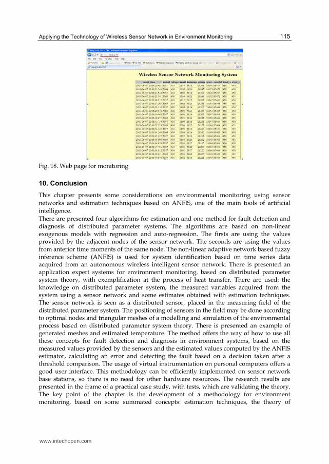
A long distance monitoring is allowed, using a web page, presented in Fig. 18.

www.intechopen.com


115

Fig. 18. Web page for monitoring

10. Conclusion

This chapter presents some considerations on environmental monitoring using sensor

networks and estimation techniques based on ANFIS, one of the main tools of artificial

intelligence.

There are presented four algorithms for estimation and one method for fault detection and diagnosis of distributed parameter systems. The algorithms are based on non-linear exogenous models with regression and auto-regression. The firsts are using the values provided by the adjacent nodes of the sensor network. The seconds are using the values from anterior time moments of the same node. The non-linear adaptive network based fuzzy inference scheme (ANFIS) is used for system identification based on time series data acquired from an autonomous wireless intelligent sensor network. There is presented an application expert systems for environment monitoring, based on distributed parameter system theory, with exemplification at the process of heat transfer. There are used: the knowledge on distributed parameter system, the measured variables acquired from the system using a sensor network and some estimates obtained with estimation techniques. The sensor network is seen as a distributed sensor, placed in the measuring field of the distributed parameter system. The positioning of sensors in the field may be done according to optimal nodes and triangular meshes of a modelling and simulation of the environmental process based on distributed parameter system theory. There is presented an example of generated meshes and estimated temperature. The method offers the way of how to use all these concepts for fault detection and diagnosis in environment systems, based on the measured values provided by the sensors and the estimated values computed by the ANFIS estimator, calculating an error and detecting the fault based on a decision taken after a threshold comparison. The usage of virtual instrumentation on personal computers offers a good user interface. This methodology can be efficiently implemented on sensor network base stations, so there is no need for other hardware resources. The research results are presented in the frame of a practical case study, with tests, which are validating the theory. The key point of the chapter is the development of a methodology for environment monitoring, based on some summated concepts: estimation techniques, the theory of

www.intechopen.com


116

distributed parameter systems, expert systems and wireless sensor networks. A negative aspect is the lack of information related to the error of measuring data, for different environment applications in practice. In future, some researches may be done in order to respond to this question related to the accuracy of measurements for different practical cases. Future applications could be done in computing interpolative values in inaccessible places from the sensor area, in the control of distributed parameter systems, and other.

11. Acknowledgement

This work was made in the frame of the CNCSIS – UEFISCSU, PNII –IDEI_PCE_ID923 grant.

12. References

Akyildiz, F.; Su, W.; Sankarasubramaniam, Y. & Cayirci, E., Wireless Sensor Networks: A Survey. Computer Networks, 38(4), March, 2002.

Cuiyun, W.; Naiang, W.; Xibao, X.; Feng, Z. & Yinzhou, H. Study on Spatial Thermal Environment in Lanzhou City Based on Remote Sensing and GIS, IEEE Int. Conf. On Geoscience and remote Sensing Symposium, July, 31, 2006, Denver, pp. 2466-1468.

Dardari, D.; Conti, A.; Buratti, C. & Verdone, R. Mathematical Evaluation of Environmental Monitoring Estimation Error through Energy-Efficient Wireless Sensor Networks, IEEE Trans. on Mobile Computing, July, 2007, Vol. 6, Issue 7, p. 790-802.

Giannopoulos, N; Goumopoulos, & Kameas, A. Design Guidelines for Building a Wireless Sensor Network for Environmental Monitoring, PCI’09 13th Panhellenic Conf. on Informatics, 10-12 Sept. 2009, Corfu, p. 148-152.

Lan, S.; Qilong, M. & Du, J. Architecture of Wireless Sensor Networks for Environmental Monitoring, GRS 2008 Int. Workshop on Geoscience and Remote Sensing, 21-22 Dec. 2008, Shanghai, Vol. 1, p. 579-582.

Rosculet, M.N. & M. Craiu, M. Differential applicative equations, RSR Academy Publishing, Bucharest,, 1979.

Talukder, A.; Panangadan, A. & Herrington, A.T. Autonomous Adaptive Resource Management in Sensor Network Systems for Environmental Monitoring, 2008 IEEE Aerospace Conf., 1-8 March 2008, Big Sky, MT, pp. 1-9.

Volosencu, C., Environmental Monitoring Based on Sensor Networks and Artificial Intelligence, Development, Energy, Environment, Economics (DEEE '10), Puerto De La Cruz, Tenerife, Nov. 30- Dec. 2, 2010, p. 79 – 83.

Volosencu, C., Algorithms for estimation in distributed parameter systems based on sensor networks and ANFIS, WSEAS Transactions on Systems, Volume 9, Issue 3, March 2010, pag. 283- 294.

www.intechopen.com

Cutting Edge Research in New TechnologiesEdited by Prof. Constantin Volosencu

ISBN 978-953-51-0463-6Hard cover, 346 pagesPublisher InTechPublished online 05, April, 2012Published in print edition April, 2012

InTech EuropeUniversity Campus STeP Ri Slavka Krautzeka 83/A 51000 Rijeka, Croatia Phone: +385 (51) 770 447 Fax: +385 (51) 686 166www.intechopen.com

InTech ChinaUnit 405, Office Block, Hotel Equatorial Shanghai No.65, Yan An Road (West), Shanghai, 200040, China

Phone: +86-21-62489820 Fax: +86-21-62489821

The book "Cutting Edge Research in New Technologies" presents the contributions of some researchers inmodern fields of technology, serving as a valuable tool for scientists, researchers, graduate students andprofessionals. The focus is on several aspects of designing and manufacturing, examining complex technicalproducts and some aspects of the development and use of industrial and service automation. The bookcovered some topics as it follows: manufacturing, machining, textile industry, CAD/CAM/CAE systems,electronic circuits, control and automation, electric drives, artificial intelligence, fuzzy logic, vision systems,neural networks, intelligent systems, wireless sensor networks, environmental technology, logistic services,transportation, intelligent security, multimedia, modeling, simulation, video techniques, water plant technology,globalization and technology. This collection of articles offers information which responds to the general goal oftechnology - how to develop manufacturing systems, methods, algorithms, how to use devices, equipments,machines or tools in order to increase the quality of the products, the human comfort or security.

How to referenceIn order to correctly reference this scholarly work, feel free to copy and paste the following:

Constantin Volosencu (2012). Applying the Technology of Wireless Sensor Network in EnvironmentMonitoring, Cutting Edge Research in New Technologies, Prof. Constantin Volosencu (Ed.), ISBN: 978-953-51-0463-6, InTech, Available from: http://www.intechopen.com/books/cutting-edge-research-in-new-technologies/applying-the-technolgy-of-wireless-sensor-networks-in-environment-monitoring-

applying the technology of wireless sensor network in...

Documents