applied databases - the university of edinburgh · applied databases. 2 outline 1. more on...

Sebastian Maneth

Lecture 8SQL and Beyond

University of Edinburgh - February 9th, 2017

Applied Databases

2

Outline

1. More on Aggregates 2. Joins 3. Limits of SQL

3

From Last Lecture

mysql> CREATE TABLE T (a INT PRIMARY KEY, b INT);mysql> INSERT INTO T VALUES(NULL,1);ERROR 1048 (23000): Column 'a' cannot be nullmysql>

MySQL is NULL allowed for a primary key attribute?

4

From Last Lecture

sqlite> CREATE TABLE T (a INT PRIMARY KEY, b INT);sqlite> INSERT INTO T VALUES(1,1);sqlite> INSERT INTO T VALUES(NULL,1);sqlite> INSERT INTO T VALUES(NULL,2);sqlite> SELECT * FROM T;1|1|1|2sqlite> SELECT a FROM T;

1sqlite> SELECT DISTINCT a FROM T;

1 sqlite>

Sqlite3

5

1. More on Aggregates

> SELECT * FROM T;+------+------+------+| a1 | a2 | a3 |+------+------+------+| a | 1 | 5 || a | 1 | 2 || a | 2 | 2 || a | 2 | 3 |+------+------+------+> SELECT a1, AVG(a3) FROM T GROUP BY a1;

??

6


> SELECT * FROM T;+------+------+------+| a1 | a2 | a3 |+------+------+------+| a | 1 | 5 || a | 1 | 2 || a | 2 | 2 || a | 2 | 3 |+------+------+------+> SELECT a1, AVG(a3) FROM T GROUP BY a1;

(1) take all a3-values and compute average: (5 + 2 + 2 + 3) / 4 = 3

(2) only (a1,a3) are relevant, so, we project onto (a1,a3) to get

+------+------+| a1 | a3 |+------+------+| a | 5 || a | 2 || a | 3 |+------+------+

average now: (5 + 2 + 3) / 3 = 10 / 3

7


> SELECT * FROM T;+------+------+------+| a1 | a2 | a3 |+------+------+------+| a | 1 | 5 || a | 1 | 2 || a | 2 | 2 || a | 2 | 3 |+------+------+------+> SELECT a1, AVG(a3) FROM T GROUP BY a1;+------+---------+| a1 | AVG(a3) |+------+---------+| a | 3.0000 |+------+---------+

→ SQL keeps duplicates

→ thus, solution (1)

8

1. More on Aggregates> SELECT * FROM T;+------+------+------+| a1 | a2 | a3 |+------+------+------+| a | 1 | 5 || a | 1 | 2 || a | 2 | 2 || a | 2 | 3 |+------+------+------+> SELECT COUNT(a3) FROM T;+-----------+| COUNT(a3) |+-----------+| 4 |+-----------+> SELECT COUNT(DISTINCT a3) FROM T; +--------------------+| COUNT(DISTINCT a3) |+--------------------+| 3 |+--------------------+> SELECT SUM(a3) FROM T;+---------+| SUM(a3) |+---------+| 12 |+---------+

> SELECT SUM(DISTINCT a3) FROM T; +------------------+| SUM(DISTINCT a3) |+------------------+| 10 |+------------------+

> SELECT MIN(a3) FROM T;

> SELECT MIN(DISTINCT a3) FROM T;

9

Selection Based on Aggregates

SELECT list, of, attributes FROM list of tablesWHERE conditionsGROUP BY list of attributesORDER BY attribute ASC | DESC

cannot contain Aggregates!

10


SELECT list, of, attributes FROM list of tablesWHERE conditionsGROUP BY list of attributesORDER BY attribute ASC | DESCHAVING AGGREGATE(attribute) operator value

→ find directors and average length of their movies, provided they made at least one movie that is longer than 2 hours

SELECT director, AVG(length) FROM MoviesGROUP BY directorHAVING MAX(length) > 120;

11


SELECT list, of, attributes FROM list of tablesWHERE conditionsGROUP BY list of attributesORDER BY attribute ASC | DESCHAVING AGGREGATE(attribute) operator value

→ find directors and average length of their movies, provided they made at least one movie that is longer than 2 hours

SELECT director, AVG(length) FROM MoviesGROUP BY directorHAVING MAX(length) > 120;

could be a nested query(e.g., selecting another aggregate!)

12


13


14


15

2. Joins

16

2. Joins

What is special about databases?

→ transaction processing (data is safe, multi-user support)→ SQL

What is special about SQL?

→ mature standard→ widely adopted & used in industry→ expressiveness and efficiency (*) all queries terminate (*) data complexity is polynomial time

What is the most important (and expensive) SQL operation?

→ the JOIN

17

2. Joins

→ for each author, find the number of papers he/she wrote

1;Sanjeev Saxena2;Hans-Ulrich Simon3;Nathan Goodman4;Oded Shmueli5;Norbert Blum6;Arnold Schonhage7;Juha Honkala8;Chua-Huang Huang9;Christian Lengauer10;Alain Finkel11;Annie Choquet12;Joachim Biskup13;Symeon Bozapalidis.

1;12;23;33;44;55;66;77;87;98;108;119;1210;1310;1410;15

paper_id author_id (aid)→ naively, takes quadratic time:

for each author, go through WrittenBy table, and count his/her number of occurrences.

Author tableWrittenBy table

18

2. Joins

→ the simplest join is just the Cartesian product.→ its size is quadratic!

SELECT * FROM Numbers;+------+| a |+------+| 1 || 2 || 3 || 4 |+------+

SELECT * FROM Numbers JOIN Numbers N2;+------+------+| a | a |+------+------+| 1 | 1 || 2 | 1 || 3 | 1 || 4 | 1 || 1 | 2 || 2 | 2 || 3 | 2 || 4 | 2 || 1 | 3 || 2 | 3 || 3 | 3 || 4 | 3 || 1 | 4 || 2 | 4 || 3 | 4 || 4 | 4 |+------+------+

19

2. Joins

→ the simplest join is just the Cartesian product.→ its size is quadratic!

SELECT * FROM Numbers, Numbers N2;+------+------+| a | a |+------+------+| 1 | 1 || 2 | 1 || 3 | 1 || 4 | 1 || 1 | 2 || 2 | 2 || 3 | 2 || 4 | 2 || 1 | 3 || 2 | 3 || 3 | 3 || 4 | 3 || 1 | 4 || 2 | 4 || 3 | 4 || 4 | 4 |+------+------+

SELECT * FROM Numbers;+------+| a |+------+| 1 || 2 || 3 || 4 |+------+

20

Co-Author Graph

1;Sanjeev Saxena2;Hans-Ulrich Simon3;Nathan Goodman4;Oded Shmueli5;Norbert Blum6;Arnold Schonhage7;Juha Honkala8;Chua-Huang Huang9;Christian Lengauer10;Alain Finkel11;Annie Choquet12;Joachim Biskup13;Symeon Bozapalidis...

1;12;23;33;44;55;66;77;87;98;108;119;1210;1310;1410;15

coauthors

3 4

aid cid.. 3 4 4 3..

How can we produce this table?

CA table =Co-Author relationship

21

Co-Author Graph1;12;23;33;44;55;66;77;87;98;108;119;1210;1310;1410;15

join using (pid)

1;12;23;33;44;55;66;77;87;98;108;119;1210;1310;1410;15

3 4

aid cid.. 3 4 4 3..

SELECT * FROM WrittenBy w1 JOIN WrittenBy w2 USING (pid);+------+------+------+| pid | aid | aid |+------+------+------+| 1 | 1 | 1 || 2 | 2 | 2 || 3 | 3 | 3 || 3 | 4 | 3 || 3 | 3 | 4 || 3 | 4 | 4 || 4 | 5 | 5 |

CA table =Co-Author relationship

22

Co-Author Graph

SELECT * FROM WrittenBy W1 JOIN WrittenBy W2 USING (pid);+------+------+------+| pid | aid | aid |+------+------+------+| 1 | 1 | 1 || 2 | 2 | 2 || 3 | 3 | 3 || 3 | 4 | 3 || 3 | 3 | 4 || 3 | 4 | 4 || 4 | 5 | 5 |

→ exclude self-relations

SELECT W1.aid,W2.aid FROM WrittenBy W1 JOIN WrittenBy W2 USING (pid)WHERE W1.aid <> W2.aid;+------+------+| aid | aid |+------+------+| 4 | 3 || 3 | 4 || 9 | 8 || 8 | 9 || 11 | 10 || 10 | 11 |

Correctly produces the Co-Author Graph!

23

2. Natural Joins

Table1 JOIN Table2 USING (c1, c2, …, cN)

→ joins all tuples of Table1 and Table2 which agree on their c1,..,cN values

→ result table has columns c1,..,cN, followed by the columns of Table1 that are not in { c1,..,cN } followed by the columns of Table2 that are not in { c1,..,cN }

SELECT * FROM T1;+------+------+------+------+| a | b | c | d |+------+------+------+------+| 1 | 2 | 3 | 1 || 4 | 5 | 6 | 2 |+------+------+------+------+SELECT * FROM T2;+------+------+| d | e |+------+------+| 1 | 1 || 1 | 2 || 2 | 4 || 2 | 7 |+------+------+

SELECT * FROM T1 JOIN T2 USING (d);+------+------+------+------+------+| d | a | b | c | e |+------+------+------+------+------+| 1 | 1 | 2 | 3 | 1 || 1 | 1 | 2 | 3 | 2 || 2 | 4 | 5 | 6 | 4 || 2 | 4 | 5 | 6 | 7 |+------+------+------+------+------+

→ order depends on implementation.(MySQL)

24

2. Joins

T1 JOIN T2 ON (T1.c1=T2.d1 AND T1.c2<=T2.d2 OR NOT( … ))

→ joins all tuples of Table1 and Table2 which satisfy join condition

→ result table has all columns of Table1 followed by all columns of Table2

SELECT * FROM T1 JOIN T2 ON (T1.d=T2.d);+------+------+------+------+------+------+| a | b | c | d | d | e |+------+------+------+------+------+------+| 1 | 2 | 3 | 1 | 1 | 1 || 1 | 2 | 3 | 1 | 1 | 2 || 4 | 5 | 6 | 2 | 2 | 4 || 4 | 5 | 6 | 2 | 2 | 7 |+------+------+------+------+------+------+

duplicate d-column

25

2. Joins→ joins are quite powerful!→ E.g. simulate GROUP BY through a join:

SELECT * FROM T;+------+| a |+------+| 1 || 1 || 2 || 2 || 2 || 3 |+------+

SELECT a,COUNT(a) FROM T GROUP BY a;+------+----------+| a | COUNT(a) |+------+----------+| 1 | 2 || 2 | 3 || 3 | 1 |+------+----------+

SELECT DISTINCT T1.a, (SELECT COUNT(T2.a) FROM T T2 WHERE T2.a=T1.a) AS Count FROM T T1;+------+-------+| a | Count |+------+-------+| 1 | 2 || 2 | 3 || 3 | 1 |+------+-------+

26

2. Joins

SELECT * FROM T;+------+| a |+------+| 1 || 1 || 2 || 2 || 2 || 3 |+------+


→ why is it a join?→ can you rewrite the query to use JOIN keyword?

→ joins are quite powerful!→ E.g. simulate GROUP BY through a join:

27

2. Joins

SELECT * FROM T;+------+| a |+------+| 1 || 1 || 2 || 2 || 2 || 3 |+------+


→ similarly, you can avoid HAVING by the use of a JOIN

→ do you see how ?

→ joins are quite powerful!→ E.g. simulate GROUP BY through a join:

28

Outer Joins

SELECT * FROM Author;+-----+------+| aid | name |+-----+------+| 1 | ab || 2 | cd || 3 | ef |+-----+------+SELECT * FROM Book;+-----+------+| bid | aid |+-----+------+| 1 | 1 || 2 | 1 || 3 | 3 |+-----+------+

SELECT * FROM Book JOIN Author USING (aid);+------+-----+------+| aid | bid | name |+------+-----+------+| 1 | 1 | ab || 1 | 2 | ab || 3 | 3 | ef |+------+-----+------+

Author “2” not listed,because he/she not in the Book-table.

29

Outer Joins


SELECT * FROM Book RIGHT OUTER JOIN Author USING (aid);+-----+------+------+| aid | name | bid |+-----+------+------+| 1 | ab | 1 || 1 | ab | 2 || 2 | cd | NULL || 3 | ef | 3 |+-----+------+------+

SELECT * FROM Book JOIN Author USING (aid);+------+-----+------+| aid | bid | name |+------+-----+------+| 1 | 1 | ab || 1 | 2 | ab || 3 | 3 | ef |+------+-----+------+

30

Outer Joins


SELECT * FROM Book RIGHT OUTER JOIN Author USING (aid);+-----+------+------+| aid | name | bid |+-----+------+------+| 1 | ab | 1 || 1 | ab | 2 || 2 | cd | NULL || 3 | ef | 3 |+-----+------+------+

SELECT aid,count(bid) AS n_books FROM Book RIGHT OUTER JOIN Author USING (aid)GROUP BY aid;+-----+---------+| aid | n_books |+-----+---------+| 1 | 2 || 2 | 0 || 3 | 1 |+-----+---------+

31

Outer Joinsmysql> SELECT * FROM T;+------+| a |+------+| 1 || 2 || 3 || NULL |+------+mysql> SELECT * FROM T, T t2;+------+------+| a | a |+------+------+| 1 | 1 || 2 | 1 || 3 | 1 || NULL | 1 || 1 | 2 || 2 | 2 || 3 | 2 || NULL | 2 || 1 | 3 || 2 | 3 || 3 | 3 || NULL | 3 || 1 | NULL || 2 | NULL || 3 | NULL || NULL | NULL |+------+------+16 rows in set (0.00 sec)

mysql> SELECT t1.a,COUNT(t2.a) FROM T t1, T t2 GROUP BY a;+------+-------------+| a | count(t2.a) |+------+-------------+| NULL | 3 || 1 | 3 || 2 | 3 || 3 | 3 |+------+-------------+

Not counted

32

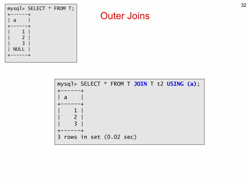
Outer Joins

mysql> SELECT * FROM T JOIN T t2 USING (a);+------+| a |+------+| 1 || 2 || 3 |+------+3 rows in set (0.02 sec)

mysql> SELECT * FROM T;+------+| a |+------+| 1 || 2 || 3 || NULL |+------+

33

Outer JoinsTable1 RIGHT OUTER JOIN Table2 USING / ON ...

→ joins all tuples of Table1 with Table2 satisfying join condition, plus all remaining tuples from Table2 (the RIGHT)

→ result tuples of the second type above have NULL-values in the columns coming from Table1.

34

Outer JoinsTable1 RIGHT OUTER JOIN Table2 USING / ON ...

→ joins all tuples of Table1 with Table2 satisfying join condition, plus all remaining tuples from Table2 (the RIGHT)


Table1 LEFT OUTER JOIN Table2 USING / ON ...

→ joins all tuples of Table1 with Table2 satisfying join condition, plus all remaining tuples from Table1 (the LEFT)


35

Outer Joins

SELECT * FROM Part;+---------+---------+| part_id | supp_id |+---------+---------+| P1 | S1 || P2 | S2 || P3 | NULL || P4 | NULL |+---------+---------+

SELECT * from Supplier;+---------+------------+| supp_id | supp_name |+---------+------------+| S1 | Supplier#1 || S2 | Supplier#2 || S3 | Supplier#3 |+---------+------------+

SELECT * FROM Part NATURAL JOIN Supplier;+---------+---------+------------+| supp_id | part_id | supp_name |+---------+---------+------------+| S1 | P1 | Supplier#1 || S2 | P2 | Supplier#2 |+---------+---------+------------+

Join on all common attributes

36

Left Outer Join

SELECT part_id,supp_name FROM Part NATURAL LEFT JOIN Supplier;+---------+------------+| part_id | supp_name |+---------+------------+| P1 | Supplier#1 || P2 | Supplier#2 || P3 | NULL || P4 | NULL |+---------+------------+



37

Right Outer Join

SELECT part_id,supp_name FROM Part NATURAL LEFT JOIN Supplier;+---------+------------+| part_id | supp_name |+---------+------------+| P1 | Supplier#1 || P2 | Supplier#2 || P3 | NULL || P4 | NULL |+---------+------------+

SELECT part_id,supp_name FROM Part NATURAL RIGHT JOIN Supplier;+---------+------------+| part_id | supp_name |+---------+------------+| P1 | Supplier#1 || P2 | Supplier#2 || NULL | Supplier#3 |+---------+------------+



38

Full Outer JoinPart NATURAL LEFT JOIN Supplier;+---------+------------+| part_id | supp_name |+---------+------------+| P1 | Supplier#1 || P2 | Supplier#2 || P3 | NULL || P4 | NULL |+---------+------------+Part NATURAL RIGHT JOIN Supplier;+---------+------------+| part_id | supp_name |+---------+------------+| P1 | Supplier#1 || P2 | Supplier#2 || NULL | Supplier#3 |+---------+------------+

Part NATURAL FULL OUTER JOIN Supplier;+---------+------------+| part_id | supp_name |+---------+------------+| P1 | Supplier#1 || P2 | Supplier#2 || P3 | NULL || P4 | NULL || NULL | Supplier#3 |+---------+------------+



39

Full Outer JoinPart NATURAL LEFT JOIN Supplier;+---------+------------+| part_id | supp_name |+---------+------------+| P1 | Supplier#1 || P2 | Supplier#2 || P3 | NULL || P4 | NULL |+---------+------------+Part NATURAL RIGHT JOIN Supplier;+---------+------------+| part_id | supp_name |+---------+------------+| P1 | Supplier#1 || P2 | Supplier#2 || NULL | Supplier#3 |+---------+------------+

Part NATURAL FULL OUTER JOIN Supplier;+---------+------------+| part_id | supp_name |+---------+------------+| P1 | Supplier#1 || P2 | Supplier#2 || P3 | NULL || P4 | NULL || NULL | Supplier#3 |+---------+------------+

→ no full outer join in mysql

→ write a query that does full outer join



40

2. Joins

→ outer joins can be useful to efficiently implement other queries!

→ efficiency of joins? (*) nested loop (*) sort merge (*) hash join

→ intermediate result sizes can be HUGE

→ query performance often depends on how you write the query! (difficult problem)

→ create indexes on all columns on which you join!

41

Sort Merge Join

1;Sanjeev Saxena2;Hans-Ulrich Simon3;Nathan Goodman4;Oded Shmueli5;Norbert Blum6;Arnold Schonhage7;Juha Honkala8;Chua-Huang Huang9;Christian Lengauer10;Alain Finkel11;Annie Choquet12;Joachim Biskup13;Symeon Bozapalidis.

1;12;23;33;44;55;66;77;87;98;108;119;1210;1310;1410;15

1;157;11089;149018;12;23784;2992;23;310193;3...

sort

already sorted

pick up join results in one top-down traversal on both tables

42

Sort Merge Join

→ a B-tree index is nothing else but a SORTED search-tree that behaves well on disk

→ even having such sorted B-tree indexes, efficient join processing remains a tremendous challenge

E.g. in which order to apply joins?

(SELECT … FROM .. ) JOIN (SELECT … FROM .. ) JOIN (SELECT … )

Smallest result?

→ histograms & approximations!

43

Sort Order

→ can cause the query to run

few seconds, or a day ...

→ absolutely crucial to determine good join order!

(SELECT … FROM .. ) JOIN (SELECT … FROM .. ) JOIN (SELECT … )

Smallest result?

→ histograms & approximations!

44

3. Limits of SQL

In a graph, determine if two given nodes A,B are connected.

45

3. Limits of SQL

In a graph, determine if two given nodes A,B are connected.

What we can do in SQL:

1) determine all nodes at distance 1 from A:

(SELECT cid FROM CA WHERE aid=A) =CA0

2) apply to this set of nodes the same query

SELECT cid FROM CA WHERE aid IN CA0 – { A } =CA1

This determines all nodes at distance two.

3) SELECT …. aid IN CA1 – CA0;

→ after k such queries we have nodes at distance k.

aid cid.. 3 4 4 3..

table CA

46

3. Limits of SQL

On the given Co-Author Graph CA (1.6 million nodes, 6.7 million edges):

→ for ONE AUTHOR feasalbe: takes ca 5 minutes (on a laptop)

But, find distance for EVERY PAIR OF AUTHORS is infeasible.

1.6 million authors.1.6 * 1.6 million numbers to compute. Storage: 2.5 TB

(probably >>1 year to compute)

SELECT 1.0*COUNT(*)/(2* (SELECT COUNT(distinct aid) from CA));4.37035511508065

47

3. Limits of SQL

→ distance for EVERY PAIR OF AUTHORS

→ is between 0 and 17

Degree Distribution?→ follows a POWER LAW! (such as Zipf Distribution!)

Average?

Mean / mode?

Power Law

node degree (= numberof outgoing edges)was computed for allnodes.

→ formulate a SQL query (over CA) that does this!

49

Power Law

y = axb

log(y) = log(a) + b log(x)

y = log(a) + bX

a line

e.g., typical Zipf could be:

NN/2N/3N/4N/5N/6...

(a = 1, b = – 1)

Power Law

Dynamics of the Co-Author Graph

SELECT DISTINCT W1.aid, W2.aid FROM Paper P, WrittenBy W1 join WrittenBy W2 on W1.pid=W2.pid WHERE W1.aid<>W2.aid ANDP.pid=W1.pid and P.year<=1955;

1955 version of CoAuthor Graph19601965...1995

Small World

“I read somewhere that everybody on this planet is separated by only six other people. Six degrees of separation. Between us and everybody else on this planet. The president of the United States. A gondolier in Venice. Fill in the names. I find that A)tremendously comforting that we're so close and B)like Chinese water torture that we're so close. Because you have to find the right six people to make the connection. It's not just big names. It's anyone. A native in a rain forest. A Tierra del Fuegan. An Eskimo. I am bound to everyone on this planet by a trail of six people. It's a profound thought. How Paul found us. How to find the man whose son he pretends to be. Or perhaps is his son, although I doubt it. How every person is a new door, opening up into other worlds. Six degrees of separation between me and everyone else on this planet. But to find the right six people.”

John Guare

Step-Wise-Reachable-Nodes (SWRN)INSERT INTO Auth(SELECT A.aid FROM Acopy A ORDER BY RANDOM() LIMIT 1)

DELETE FROM CA1;INSERT INTO CA1 SELECT DISTINCT C.cid FROM CA C, CA0 DWHERE D.aid=C.aid AND C.cid NOT IN (SELECT E.aid FROM CA0 E);

INSERT INTO Adist SELECT Auth.aid,Counter.i,COUNT(C.cid)FROM Auth,Counter, CA1 C;

INSERT INTO CA0 SELECT * FROM CA1;UPDATE Counter SET i=(SELECT Counter.i+1 FROM Counter);

repeat untilCA1 becomesempty

at most 17-times(longest distance in the graph)

Adist table1513 | 1 | 651513 | 2 | 1,5991513 | 3 | 37,7481513 | 4 | 407,8391513 | 5 | 665,4051513 | 6 | 223,9571513 | 7 | 4,37581513 | 8 | 8,6841513 | 9 | 1904. 13| 11

Degrees of Separation in the DPLP Co-Author Graph

→ obtained by running SWRN (≤17)on a random sampleof 50 nodes.

→ what “confidence” does the sample give?

DPLP Co-Author Graph

$ Rscript.exe do_stats.RDistance Frequency Distribution -- Summary: mean median mode var sd5.941985 6.000000 6.000000 1.256740 1.121044Coverage of largest component (in %): [1] 73.0216Percentage reached after 5 hops (in that component): [1] 35.10105Percentage reached after 6 hops (in that component): [1] 72.53906

64

ENDLecture 8

applied databases - the university of edinburgh · applied databases. 2 outline 1. more on...

Documents