Disclosure Limitation in Large Statistical Databases

Stephen F. Roehrig

CMU/Pitt Applied Decision Modeling Seminar

Collaborators George Duncan, Heinz/Statistics, CMU Stephen Fienberg, Statistics, CMU Adrian Dobra, Statistics, Duke Larry Cox, Center for Health Statistics,

H&HS Jesus De Loera, Math, UC Davis Bernd Sturmfels, Math, UC Berkeley JoAnne O’Roarke, Institute for Social

Research, U. Michigan

Funding NSF NCES NIA NCHS NISS Census BLS

How Should Government Distribute What It Knows?

Individuals and businesses contribute data about themselves, as mandated by government

Government summarizes and returns these data to policy makers, policy researchers, individuals and businesses

Everyone is supposed to see the value, but with no privacy downside Obligations: return as much information as

possible Restrictions: don’t disclose sensitive

information

Who Collects Data? Federal, state and local government:

Census Bureau of Labor Statistics National Center for Health Statistics, etc.

Federally funded surveys: Health and Retirement Study (NIA) Treatment Episode Data Set (NIH)

Industry Health care Insurance “Dataminers”

Real-World Example I The U.S. Census Bureau wants to allow

online queries against its census data. It builds a large system, with many

safeguards, then calls in “distinguished university statisticians” to test it.

Acting as “data attackers”, they attempt to discover sensitive information.

They do, and so the Census Bureau’s plans must be scaled back.

(Source: Duncan, Roehrig and Kannan)

Real-World Example II To better understand health care usage

patterns, a researcher wants to measure the distance from patients’ residences to the hospitals where their care was given.

But because of confidentiality concerns, it’s only possible to get the patients’ ZIP codes, not addresses.

The researcher uses ZIP code centroids instead of addresses, causing large errors in the analysis.

(Source: Marty Gaynor)

Real-World Example III To understand price structures in the

health care industry, a researcher wants to compare negotiated prices to list prices, for health services.

One data set has hospital IDs and list prices for various services. Another data set gives negotiated prices for actual services provided, but for for confidentiality reasons, no hospital IDs can be provided.

Thus matching is impossible.(Source: Marty Gaynor)

Data Utility vs. Disclosure Risk Data utility: a measure of the usefulness

of a data set to its intended users Disclosure risk: the degree to which a

data set reveals sensitive information The tradeoff is a hard one, currently

judged mostly heuristically Disclosure limitation, in theory and

practice, examines this tradeoff.

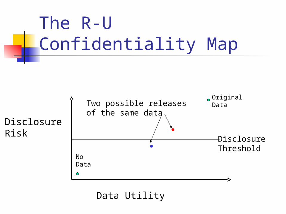
The R-U Confidentiality Map

Data Utility

DisclosureRisk

DisclosureThreshold

OriginalData

NoData

Two possible releasesof the same data

The R-U Confidentiality Map

Data Utility

DisclosureRisk

DisclosureThreshold

DL Method 1

DL Method 2

OriginalData

NoData

For many disclosure limitation methods, we canchoose one or more parameters.

Traditional Methods: Microdata Microdata: a set of records containing

information on individual respondents Suppose you are supposed to release

microdata, for the public good, about individuals. The data include: Name Address City of residence Occupation Criminal record

Microdata Typical safeguard: delete

“identifiers” So release a dataset containing only city

of residence, occupation and criminal record…

Microdata Typical safeguard: delete

“identifiers” So release a dataset containing only city

of residence, occupation and criminal record… Residence = Amsterdam Occupation = Mayor Criminal history = has criminal record

Microdata Typical safeguard: delete “identifiers” So release a dataset containing only city of

residence, occupation and criminal record… Residence = Amsterdam Occupation = Mayor Criminal history = has criminal record

HIPPA says this is OK, so long as a researcher “promises not to attempt re-identification”

Is this far-fetched?

Microdata Unique (or almost unique)

identifiers are common The 1997 voting list for Cambridge,

MA has 54,805 voters:

birth date alone 12%birth date and gender 29%birth date and 5-digit ZIP 69%birth date and full postal code 97%

Uniqueness of demographic fields

(Source: Latanya Sweeney)

Traditional Solutions for Microdata Sampling Adding noise Global recoding (coarsening) Local suppression Data swapping Micro-aggregation

Example: Data SwappingLocation Age Sex Candidate

Pittsburgh Young M Bush

Pittsburgh Young M Gore

Pittsburgh Young F Gore

Pittsburgh Old M Gore

Pittsburgh Old M Bush

Cleveland Young F Bush

Cleveland Young F Gore

Cleveland Old M Gore

Cleveland Old F Bush

Cleveland Old F Gore

Unique on location,age and sex

Find a match in another location

Flip a coin to seeif swapping is done

Data Swapping Terms Uniques Key: Variables that are used to

identify records that pose a confidentiality risk.  

Swapping Key: Variables that are used to identify which records will be swapped.

Swapping Attribute: Variables over which swapping will occur.

Protected Variables: Other variables, which may or may not be sensitive.

Location Age Sex Candidate

Pittsburgh Young M Bush

Pittsburgh Young M Gore

Pittsburgh Young F Gore

Pittsburgh Old M Gore

Pittsburgh Old M Bush

Cleveland Young F Bush

Cleveland Young F Gore

Cleveland Old M Gore

Cleveland Old F Bush

Cleveland Old F Gore

Uniques Key &Swapping Key

SwappingAttribute

ProtectedVariable

Data Swapping In Use The Treatment Episode Data Set

(TEDS) National admissions to drug treatment

facilities Administered by SAMHSA (part of HHS) Data released through ICPSR 1,477,884 records in 1997, of an

estimated 2,207,375 total admissions nationwide

TEDS (cont.) Each record contains

Age Sex Race Ethnicity Education level Marital status Source of income State & PMSA Primary substance abused and much more…

First Step: Recode Example recode: Education level

Continuous 0-25

1: 8 years or less2: 9-113: 124: 13-155: 16 or more

becomes

TEDS Uniques Key This was determined empirically,after

recoding. We ended up choosing: State and PMSA Pregnancy Veteran status Methadone planned as part of treatment Race Ethnicity Sex Age

Other Choices Swapping key: the uniques key,

plus primary substance of abuse Swapping attribute: state, PMSA,

Census Region and Census Division Protected variables: all other TEDS

variables

TEDS Results After recoding, only 0.3% of the

records needed to be swapped Swapping was done between

nearby locations, to preserve statistics over natural geographic aggregations

Tables: Magnitude Data

Language Region A Region B Region C TotalC++ 11 47 58 116Java 1 15 33 49Smalltalk 2 31 20 53Total 14 93 111 218

Profit of Software Firms $10 million(Source: Java Random.nextInt(75))

Tables: Frequency Data

Race $10,000 >$10,000 and $25,000 > $25,000 TotalWhite 96 72 161 329Black 10 7 6 23Chinese 1 1 2 4Total 107 80 169 356

Income Level, Gender = Male

Race $10,000 >$10,000 and $25,000 > $25,000 TotalWhite 186 127 51 364Black 11 7 3 21Chinese 0 1 0 1Total 197 135 51 386

Income Level, Gender = Female

(Source: 1990 Census)

Traditional Solutions for Tables Suppress some cells

Publish only the marginal totals Suppress the sensitive cells, plus others as

necessary Perturb some cells

Controlled rounding Lots of research here, and good results

for 2-way tables For 3-way and higher, this is surprisingly

hard!

Disclosure Risk, Data Utility Risk

the degree to which confidentiality might be compromised

perhaps examine cell feasibility intervals, or better, distributions of possible cell values

Utility a measure of the value to a legitimate user higher, the more accurately a user can

estimate magnitude of errors in analysis based on the released table

Example: Delinquent Children

County Low Medium High Very High

Total

Alpha 15 1 3 1 20

Beta 20 10 10 15 55

Gamma 3 10 10 2 25

Delta 12 14 7 2 35

Total 50 35 30 20 135

Education Level of Head of Household

Number of Delinquent Children by County and Education Level(Source: OMB Statistical Policy Working Paper 22)

Controlled Rounding (Base 3)

Uniform (and known) feasibility interval. Easy for 2-D tables, sometimes impossible for 3-D 1,025,908,683 possible original tables.

County Low Medium High Very High

Total

Alpha 15 0 3 0 18

Beta 21 9 12 15 57

Gamma 3 9 9 3 24

Delta 12 15 6 3 36

Total 51 33 30 21 135

Suppress Sensitive Cells & Others

Hard to do optimally (NP complete). Feasibility intervals easily found with LP. Users have no way of finding cell value

probabilities.

County Low Medium High Very High

Total

Alpha 15 p s p 20

Beta 20 10 10 15 55

Gamma 3 10 s p 25

Delta 12 s 7 p 35

Total 50 35 30 20 135

Release Only the Margins

County Low Medium High Very High

Total

Alpha 20

Beta 55

Gamma 25

Delta 35

Total 50 35 30 20 135

Release Only the Margins 18,272,363,056 tables have our margins

(thanks to De Loera & Sturmfels). Low risk, low utility. Easy! Very commonly done. Statistical users might estimate internal

cells with e.g., iterative proportional fitting.

Or with more powerful methods…

Some New Methods for Disclosure Detection Use methods from commutative algebra

to explore the set of tables having known margins

Originated with the Diaconis-Sturmfels paper (Annals of Statistics, 1998)

Extensions and complements by Dobra and Fienberg

Related to existing ideas in combinatorics

Background: Algebraic Ideals

Let A be a ring (e.g., ℝ or ℤ), and I A. Then I is called an ideal if 0 I If f, g I, then f + g I If f I and h A, then f h I

Ex. 1: The ring ℤ of integers, and the set

I = {…-4, -2, 0, 2, 4,…}.

AIfg h

Generators Let f1,…,fs A. Then

is the ideal generated by f1,…,fs

Ex. 1: The ring ℤ of integers, and the set I = {…-4, -2, 0, 2, 4,…}. SAT question: What is a generator of I ? I = 2, since I = {2} {…-1, 0, 1,…}

Ahhfhff si

s

iis ,,:,, 1

11

Ideal Example 2 The ring k [x] of polynomials of one

variable, and the ideal I = x 4-1, x 6-1.

GRE question: What is a minimal generator of I (i.e., no subset also a generator)?

I = x 2-1 since x 2-1 is the greatest common divisor of {x 4-1, x 6-1}.

Why Are Minimal Generators Useful? Compact representation of the

ideal---the initial description may be “verbose”.

Allow easy generation of elements, often in a disciplined order.

Guaranteed to explore the full ideal.

Disclosure Analysis: Marginals Suppose a “data snooper” knows

only this:

County Low Medium High Very High

Total

Alpha 20

Beta 55

Gamma 25

Delta 35

Total 50 35 30 20 135

Disclosure Analysis Of course the data collector knows

the true counts:

County Low Medium High Very High

Total

Alpha 15 1 3 1 20

Beta 20 10 10 15 55

Gamma 3 10 10 2 25

Delta 12 14 7 2 35

Total 50 35 30 20 135

Disclosure Analysis What are the feasible tables, given

the margins? Here is one:

County Low Medium High Very High

Total

Alpha 15+1 1-1 3 1 20

Beta 20-1 10+1 10 15 55

Gamma 3 10 10 2 25

Delta 12 14 7 2 35

Total 50 35 30 20 135

Disclosure Analysis Problems Both the data collector and the snooper

are interested in the largest and smallest feasible values for each cell. Narrow bounds might constitute disclosure.

Both might also be interested in the distribution of possible cell values. A tight distribution might constitute

disclosure.

The Bounds Problem

0 1 2 3 4 5

County Low Medium High Very High

Total

Alpha 20

Beta 55

Gamma 25

Delta 35

Total 50 35 30 20 135

This is usually framedas a continuous problem.Is this the right question?

The Distribution Problem

0 1 2 3 4 5

County Low Medium High Very High

Total

Alpha 20

Beta 55

Gamma 25

Delta 35

Total 50 35 30 20 135

Given the margins, anda set of priors over cellvalues, what distributionresults?

Transform to an Algebraic Problem Define some indeterminates:

Then write the move

as the polynomial x11x22 - x12x21

x1

1

x1

2

x1

3

x1

4

x2

1

x2

2

x2

3

x2

4

x3

1

x3

2

x3

3

x3

4

x4

1

x4

2

x4

3

x4

4

1 -1

-1 1

Ideal Example 3 Ideal I is the set of monomial differences

that take a non-negative table of dimension

J K with fixed margins M to another non-negative table with the same margins.

Putnam Competition question: What is a minimal generator of I ?

JKJK mJK

mnJK

n xxxx 11

11

Solutions: Bounds, Distributions Upper and lower bounds on cells:

Integer linear programming (max/min, subject to constraints implied by the marginals).

Find a generator of the ideal: Use Buchberger’s algorithm to find a Gröbner basis. Apply long division repeatedly; the remainder yields

an optimum (Conti & Traverso).

Distribution of cell values: Use the Gröbner basis to enumerate or sample

(Diaconis & Sturmfels, Dobra, Dobra & Fienberg).

Trouble in Paradise For larger disclosure problems

(dimension 3), the linear programming bounds may be fractional.

For larger disclosure problems (dimension 3), the Gröbner basis is very hard to compute.

Why Fractional Bounds? Sometimes the marginal sum

values cause the constraints to intersect at non-integer points.

x2

x1

LP maximum for x2

Integer maximum

But Could This Happen? Standard example from ManSci

101:

x2

x1

LP maximum for x2

Integer maximum

Computing Gröbner Bases Both the Conti & Traverso and Sturmfels

constructions include extra variables. The ring k [x1,…,xIJK] is embedded in

k [x1,…,xIJK, y1,…,yN], where N is the number of constraints.

Buchberger’s algorithm applied. Then throw away basis elements not in k[x1,

…,xIJK] Computing a basis for the 333

problem: about 7 hours with Macaulay.

An Improved Algorithm Designed to compute implicitly in k [x1,…,xIJK, y1,…,yN] but only

process elements in k [x1,…,xIJK].

An Improved Algorithm Designed to compute implicitly in k [x1,…,xIJK, y1,…,yN] but only

process elements in k [x1,…,xIJK]. 333 problem runs in 25 mS.

An Improved Algorithm Designed to compute implicitly in k [x1,…,xIJK, y1,…,yN] but only

process elements in k [x1,…,xIJK]. 333 problem runs in 25 mS. 433 problem runs in 20 min.

An Improved Algorithm Designed to compute implicitly in k [x1,…,xIJK, y1,…,yN] but only

process elements in k [x1,…,xIJK]. 333 problem runs in 25 mS. 433 problem runs in 20 min. 533 problem runs in 3 months…

Ideals

“If they’re so freaking ideal, how come you can’t compute them?” Overheard at Grostat 5, the

Conference on Commutative Algebra and Statistics.

Other Approaches Connections with decomposable and

graphical log-linear models (Dobra & Fienberg, Dobra).

Example: 3-D sensitive table, two 2-D margins given. Use conditional independence:

A B C

Known margins

A

B

C

Decomposable Models Gröbner bases are “simple,” and

can be written down explicitly. For some other problems (e.g.,

graphical models), the Gröbner basis can be “assembled” from bases for smaller pieces.

Nice!

A New Method for Disclosure Limitation: Cyclic Perturbation Choose cycles that leave the

margins fixed. One example:

The set of cycles determines the published table’s feasibility interval

15 1 3 120 10 10 15 3 10 10 212 14 7 2

+ 1 0 -1 0 -1 0 1 0 0 0 0 0 0 0 0 0

16 1 2 119 10 11 15 3 10 10 212 14 7 2

=

Original Cycle Perturbed table

Cyclic Perturbation: Details Choose a set of cycles that covers

all table cells “equally”. Example:

+ - 0 0 0 + - 0 0 0 + - - 0 0 +

0 + - 0 0 0 + - - 0 0 + + - 0 +

0 0 + - - 0 0 + + - 0 0 0 + - 0

- 0 0 + + - 0 0 0 + - 0 0 0 + -

Each cell has exactlytwo “chances” to move.

Cyclic Perturbation: Details

Flip a three-sided coin with outcomes A (probability = ) B (probability = ) C (probability = )

If A, add the first cycle (unless there is a zero in the cycle)

If B, subtract the first cycle (unless there is a zero in the cycle)

If C, do nothing Repeat with the remaining cycles

Cyclic Perturbation: Details For the chosen set of cycles, there

are 34=81 possible perturbed tables.

The feasibility interval is original value 2.TO

TPPerturbed

Table

Original

Table

cycle 1applied

cycle 2applied

cycle 3applied

cycle 4applied

Cyclic Perturbation: Details Choose , . Perturb with each cycle. Publish the resulting table. Publish the cycles and , .

15 1 3 120 10 10 15 3 10 10 212 14 7 2

16 0 2 221 11 9 14 2 11 11 111 13 8 3

Original Perturbed table

Analysis of Cell Probabilities

TO

TP

TO

T4

Tk

OriginalTable

PerturbedTable

PossibleTables

Distributions of Cell Values Since the mechanism is public, a user can

calculate the distribution of true cell values: Compute every table Tk that could have been

the original, along with the probability Pr(TP | Tk).

Specify a prior distribution over all the possible original tables Tk.

Apply Bayes’ theorem to get the posterior probability Pr(Tk | TP) for each Tk.

The distribution for each cell is

qjitk

Pk

k

TTqjit),(:

)|Pr()),(Pr(

Results for the Example

Pr( t(1,2) = q | TP ) 0.71 0.25 0.04 0.00 0.00 0.00Pr( t(1,4) = q | TP ) 0.06 0.25 0.38 0.25 0.06 0.00Pr( t(3,4) = q | TP ) 0.00 0.71 0.25 0.04 0.00 0.00Pr( t(4,4) = q | TP ) 0.00 0.05 0.29 0.44 0.21 0.01

q = 0 1 2 3 4 5

15 1 3 120 10 10 15 3 10 10 212 14 7 2

Original Perturbed table

16 0 2 221 11 9 14 2 11 11 111 13 8 3

Properties It’s not difficult to quantify data

utility and disclosure risk (cf. cell suppression and controlled rounding).

Priors of data users and data intruders can be different.

Theorem: For a uniform prior, the mode of each posterior cell distribution is it’s published value.

Scaling Sets of cycles w/ desirable properties

are easy to find for larger 2-D tables. Extensions to 3 and higher dimensions

also straightforward. Computing the perturbation for any size

table is easy & fast. The complete Bayesian analysis is

feasible to at least 2020 (with no special TLC)

What Might Priors Be? They could reflect historical data. If I’m in the survey, I know my cell

is at least 1. Public information. Insider information.

Rounding Redux A similar Bayesian analysis can be done,

provided the exact algorithm is available. It’s generally much harder to do. Using a deterministic version of Cox’s `87

rounding procedure, we must consider “only” 17,132,236 tables.

For uniform priors, the posterior cell distributions were nearly uniform.

Three days of computing time for a 44 table…

Future Work (i.e. What’s Hot?) Much more to be learned about the

connections between log-linear models, algebraic structures and networks.

The Grostat conference, and the “Tables” conference at Davis have resulted in wonderful collaborations between statisticians, mathematicians and operations researchers.

Stay tuned!