application to acoustic echo...

OPTIMAL ALGORITHMS FOR BLIND SOURCE SEPARATION

--- APPLICATION TO ACOUSTIC ECHO CANCELLATION

A Dissertation Submitted

For the Degree of

M.Eng.Sci

By

Ye Liang

Head of Department: Dr. Seán McLoone

Supervisor of Research: Dr. Bob Lawlor

Department of Electronic Engineering

National University Of Ireland, Maynooth

. September 2010.

ii

Abstract

We are all familiar with the sound which can be viewed as a wave motion in air or other

elastic media. In this case, sound is a stimulus. Sound can also be viewed as an excitation

of the hearing mechanism that results in the perception of sound. The interaction between

the physical properties of sound, and our perception of them, poses delicate and complex

issues. It is this complexity in audio and acoustics that creates such interesting problems.

Acoustic echo is inevitable whenever a speaker is placed near to a microphone in a

general full-duplex communication application. The most common communication

scenario is the hands-free mobile communication kits for a car. For example, the voice

from the loudspeaker is unavoidably picked up by the microphone and transmitted back

to the remote speaker. This makes the remote speaker hear his/her own voice distorted

and delayed by the communication channel or called end to end delay, which is known as

echo. Obviously, the longer the channel delay, the more annoying the echo resulting a

decrease in the perceived quality of the communication service such as VoIP conference

call.

In the thesis, we propose to use different approaches to perform acoustic echo

cancellation. In addition, we exploit the idea of blind source separation (BSS) which can

estimate source signals using only information about their mixtures observed in each

input signal. In addition, we provide a wide theoretical analysis of models and

algorithmic aspects of the widely used adaptive algorithm Least Mean Square (LMS).

We compare these with Non-negative Matrix Factorization (NMF), and their various

extensions and modifications, especially for the purpose of performing AEC by

employing techniques developed for monaural sound source separation.

iii

Acknowledgement

This thesis would not be what it is without the help, encouragement and friendship of

many people, so now is the time to give credit where credit is due.

I would like to thank my principal supervisor, Dr. Bob Lawlor, for all his patience,

guidance, support and encouragement, especially for all the times when I’m sure it

seemed like this research was going nowhere. He was always there to meet and talk

about my ideas, and to ask me good questions to help me think through my project.

Without his encouragement and constant guidance, I could not have finished my project.

He helped me all the time through the project and also provided me with constructive

feedback on my project report.

I would like to thank Mr Niall Cahill for his technical support. He has been actively

involved in many aspect of this project, and he helped me with the development of the

algorithm and experiments. I would like to thank Xin Zhou for the help in demonstrating

experiments and record the results. I would like to thank the administrative staff, Miss.

Joanna O’Grady, for her assistance support through my study. I would also like to thank

all my colleagues from the Electronic Engineering department NUI Maynooth for their

support and for their contributions to this work.

Finally I would like to thank my parents and my family members all their

encouragement throughout the years. I would also like to thank my friends in Ireland, my

landlord Mr Patrick Kavanagh, for looking after me throughout the years.

iv

Publication Arising From This Work

• Zhou X., Liang Y., Cahill N., Lawlor R., “Using Convolutive Non-negative

Matrix Factorization Algorithm To Perform Acoustic Echo Cancellation”, NUI

Maynooth, China-Ireland Conference on Information and Communication

Technologies, August 19th -21st 2009, Maynooth

v

Table of Contents

ABSTRACT II

ACKNOWLEDGEMENT III

PUBLICATION ARISING FROM THIS WORK IV

TABLE OF CONTENTS V

LIST OF FIGURES IX

LIST OF TABLES XI

ACRONYMS XII

1. INTRODUCTION 1

1.1 Research problem description 1

1.2 Thesis organization and overview 2

2. ACOUSTIC BLIND SOURCE SEPARATION BACKGROUND AND THEORY 4

2.1 BSS Generative Model 4

2.1.1 Instantaneous mixture model 5

2.1.2 Convolutive mixture model 6

2.2 Speech source signal characteristics and BSS criteria 7

2.2.1 Basic signal properties of acoustic signals 7

2.2.2 Criteria for BSS in Speech Separation 8

2.3 Acoustic echo cancellation 9

2.3.1 General Principle 9

2.3.2 Joint Blind Source Separation and Echo Cancellation 10

2.3.3 Limitation of conventional Acoustic Echo Canceller 14

2.3.4 Conclusions 14

3 OPTIMUM ALGORITHMS FOR BLIND SOURCE SEPARATION 15

3.1 Independent Component Analysis (ICA) 15

3.1.1 Background Theory of Independent Component Analysis 15

3.1.2 Notation of Blind Source Separation 16

3.1.3 Definition of ICA 17

3.1.4 Restrictions in ICA 18

3.1.5 Background theory of ICA 19

3.2 Principal Component Analysis (PCA) 21

vi

3.2.1 Introduction 21

3.2.2 Mathematics Background 22

3.2.3 PCA Methodology 23

3.2.4 Procedure of PCA 24

3.3 Degenerate unmixing estimation technique (DUET) 27

3.3.1 Introduction to DUET 27

3.3.2 Sources assumptions and mathematics background 28

3.3.3 Local stationarity and Microphones close together 30

3.3.4 DUET demixing model and parameters 30

3.3.5 Construction of the 2D weighted histogram 31

3.3.6 Maximum-likelihood (ML) estimators 32

3.3.7 Summary of DUET Algorithm 33

3.4 Azimuth Discrimination and Resynthesis 34

3.4.1 Background and Introduction 34

3.4.2 ADRess Methodology 35

3.4.3 Problem with ADRess 38

3.4.4 Resynthesis 39

3.5 Conclusions 40

4. NMF ALGORITHM 42

4.1 Introduction 42

4.2 Cost function 42

4.3 Initialization of NMF 45

4.3.1 Optimization problem 45

4.3.2 Basic initialization for NMF algorithm 46

4.3.3 Termination condition 47

4.4 Convolutive NMF 48

4.5 Conclusions 50

5. ACOUSTIC ECHO CANCELLATION MATLAB EXPERIMENT 52

5.1 Least Mean Square Solution for Acoustic Echo Cancellation 52

5.1.1 Steepest Decent Algorithm 52

5.1.2 LMS Derivation 53

5.1.3 Gradient behaviour 53

5.1.4 Condition for the LMS convergence 53

5.1.5 Rate of convergence of LMS algorithm 55

5.1.6 Steps associated with the NLMS algorithm 56

5.1.7 Excess Mean-Square Error and Misadjustment 57

5.2 Using different LMS Algorithms to Perform AEC 58

5.2.1 Experiment principles and procedure 58

5.2.2 LMS and NLMS Simulation Results 60

5.2.3 FastLMS and NFastLMS Simulation Results 63

5.2.4 Summary of the performance of LMS algorithm 67

5.3 Using NMF to Perform AEC 68

vii

5.3.1 Experiment Principle and procedure 68

5.3.2 Conventional NMF Simulation results 69

5.3.3 Convolutive NMF Simulation Results 73

5.4 Measurement results 76

5.5 Discussion and conclusions 77

6. REAL TIME HARDWARE IMPLEMENTATION 80

6.1 Introduction 80

6.2 Workstation setup and hardware profile 80

6.3 Real-time application setup 82

6.3.1 RTDX Technology 82

6.3.2 RTDX Link to MATLAB 82

6.4 Speech recognition Implementation 82

6.5 Echo control Implementation 83

6.5.1 On board stereo codec for input and output 83

6.5.2 Modifying program to create an echo 85

6.5.3 Modifying program to create an echo control 86

6.6 Notes and Conclusions 87

7. CONCLUSION AND FUTURE WORK 88

7.1 Future work 88

ACKNOWLEDGEMENTS 89

APPENDIX A: 90

Least Mean Square MATLAB Script: 90

Normalized Least Mean Square MATLAB Script: 91

Fast Least Mean Square MATLAB Script: 92

ERLE Function MATLAB Script: 94

Convolutive NMF MATLAB Script: 95

Objective Measure MATLAB Script: 100

Resynthesis MATLAB Script: 103

APPENDIX B: 104

TI C6713 DSK MAIN C PROGRAM IMPLEMENTATION 104

viii

echo.c echo with fixed delay and feedback 104

echo_control.c echo with variable delay and feedback 105

BIBLIOGRAPHY 106

ix

List of Figures

FIGURE 2.1: BLOCK DIAGRAM OF THE INSTANTANEOUS BSS TASK ...................................... 5

FIGURE 2.2: BLOCK DIAGRAM OF THE CONVOLUTIVE BSS TASK .......................................... 6

FIGURE 2.3: LINE ECHO CANCELLER INTEGRATION FLOW DIAGRAM .................................. 11

FIGURE 2.4: STRUCTURE OF ACOUSTIC ECHO CANCELLER IN THE ROOM ENVIRONMENT ... 12

FIGURE 2.5: ECHO CANCELLATION FOLLOWED BY BLIND SIGNAL SEPARATION ................. 13

FIGURE 3.1: MODEL OF BLIND SOURCE SEPARATION ......................................................... 15

FIGURE 3.2: BLOCK DIAGRAMS ILLUSTRATING BLIND SIGNAL PROCESSING PROBLEM ...... 16

FIGURE 3.3: MUTUAL INFORMATION BETWEEN TWO RANDOM VARIABLES ........................ 19

FIGURE 3.4A: ORIGINAL TWO DIMENSIONAL DATA ............................................................. 26

FIGURE 3.4B: NORMALIZED TWO DIMENSIONAL DATA ...................................................... 26

FIGURE 3.4C: DATA BY APPLYING THE PCA ANALYSIS USING BOTH EIGENVECTORS ........ 27

FIGURE 3.4D: THE RECONSTRUCTION FROM THE DATA THAT WAS DERIVED USING ONLY A

SINGLE EIGENVECTOR .................................................................................................. 27

FIGURE 3.5: DUET TWO-DIMENSIONAL CROSS POWER WEIGHTED HISTOGRAM OF

SYMMETRIC ATTENUATION .......................................................................................... 32

FIGURE 3.6: ILLUSTRATION OF INTERAURAL INTENSITY DIFFERENCE ............................... 34

FIGURE 3.7: FREQUENCY-AZIMUTH PLANE. PHASE CANCELLATION HAS OCCURRED WHERE

THE NULLS APPEAR AS SHOWN. ................................................................................... 37

FIGURE 3.8: BY INVERTING THE NULLS OF THE FREQUENCY AZIMUTH COMPOSITION THE

FREQUENCY COMPOSITION OF EACH SCORE CAN BE CLEARLY SEEN ........................... 37

FIGURE 3.9: THE PLOT DISPLAYS THE ENERGY DISTRIBUTION OF SOURCE ACROSS THE

STEREO FILED WITH RESPECT TO TIME. ........................................................................ 38

FIGURE 4.1: ILLUSTRATION OF CONVOLUTION NMF .......................................................... 48

FIGURE 5.1: AEC OPERATION IN THE ROOMACOUSTIC ENVIRONEMENT ............................. 59

FIGURE 5.2: ECHO CANCELLATION RESULTS PERFORMED BY LMS AND NLMS ................ 62

FIGURE 5.3: ERLE VALUE COMPARISON (LMS VS. NLMS) ................................................ 63

FIGURE 5.4: ECHO CANCELLATION RESULTS PERFORMED BY FAST LMS ........................... 65

FIGURE 5.5: ERLE VALUE COMPARISON (FLMS VS. NFLMS)............................................ 65

FIGURE 5.6: THE SPECTRUMGRAM OF RESIDUAL ECHO USING FAST LMS WITHOUT

NORMALIZATION .......................................................................................................... 66

FIGURE 5.7: THE SPECTRUMGRAM OF RESIDUAL ECHO USING FAST LMS WITH

NORMALIZATION .......................................................................................................... 67

FIGURE 5.8: NEAR-END SPEECH WITH NOISY PAUSE WAVEFORM........................................ 71

FIGURE 5.9: FAR-END NOISE SPEECH WAVEFORM ............................................................... 72

FIGURE 5.10: MIXTURE ECHO AND NEAR-END SPEECH BEFORE NMF PROCESSING ............ 72

x

FIGURE 5.11: MIXTURE ECHO AND NEAR-END SPEECH AFTER NMF PROCESSING .............. 73

FIGURE 5.12: NEAR-END SPEECH (WITH PAUSE) WAVEFORM ............................................. 74

FIGURE 5.13: FAR-END NOISE SPEECH WAVEFORM ............................................................. 75

FIGURE 5.14: MIXTURE ECHO AND NEAR-END SPEECH BEFORE CNMF PROCESSING ......... 75

FIGURE 5.15: MIXTURE ECHO AND NEAR-END SPEECH AFTER CNMF PROCESSING ........... 76

FIGURE 6.1: TMS3206713-BASED DSK BOARD: (A) PHYSICAL BOARD AND (B) BLOCK

DIAGRAM ..................................................................................................................... 81

FIGURE 6.2 STEPS FOR SPEECH RECOGNITION IMPLEMENTATION ....................................... 83

FIGURE 6.3: SIMPLE BLOCK DIAGRAM REPRESENTION OF FADING ECHO PROGRAM ........... 86

xi

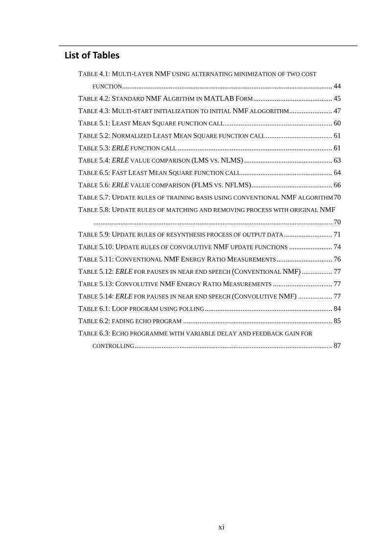
List of Tables

TABLE 4.1: MULTI -LAYER NMF USING ALTERNATING MINIMIZATION OF TWO COST

FUNCTION..................................................................................................................... 44

TABLE 4.2: STANDARD NMF ALGRITHM IN MATLAB FORM ............................................ 45

TABLE 4.3: MULTI -START INITIALIZATION TO INITIAL NMF ALOGORITHM ........................ 47

TABLE 5.1: LEAST MEAN SQUARE FUNCTION CALL ............................................................ 60

TABLE 5.2: NORMALIZED LEAST MEAN SQUARE FUNCTION CALL ..................................... 61

TABLE 5.3: ERLE FUNCTION CALL ...................................................................................... 61

TABLE 5.4: ERLE VALUE COMPARISON (LMS VS. NLMS) ................................................. 63

TABLE 6.5: FAST LEAST MEAN SQUARE FUNCTION CALL................................................... 64

TABLE 5.6: ERLE VALUE COMPARISON (FLMS VS. NFLMS) ............................................. 66

TABLE 5.7: UPDATE RULES OF TRAINING BASIS USING CONVENTIONAL NMF ALGORITHM 70

TABLE 5.8: UPDATE RULES OF MATCHING AND REMOVING PROCESS WITH ORIGINAL NMF

..................................................................................................................................... 70

TABLE 5.9: UPDATE RULES OF RESYNTHESIS PROCESS OF OUTPUT DATA ........................... 71

TABLE 5.10: UPDATE RULES OF CONVOLUTIVE NMF UPDATE FUNCTIONS ........................ 74

TABLE 5.11: CONVENTIONAL NMF ENERGY RATIO MEASUREMENTS ............................... 76

TABLE 5.12: ERLE FOR PAUSES IN NEAR END SPEECH (CONVENTIONAL NMF) ................. 77

TABLE 5.13: CONVOLUTIVE NMF ENERGY RATIO MEASUREMENTS ................................. 77

TABLE 5.14: ERLE FOR PAUSES IN NEAR END SPEECH (CONVOLUTIVE NMF) ................... 77

TABLE 6.1: LOOP PROGRAM USING POLLING ....................................................................... 84

TABLE 6.2: FADING ECHO PROGRAM ................................................................................... 85

TABLE 6.3: ECHO PROGRAMME WITH VARIABLE DELAY AND FEEDBACK GAIN FOR

CONTROLLING .............................................................................................................. 87

xii

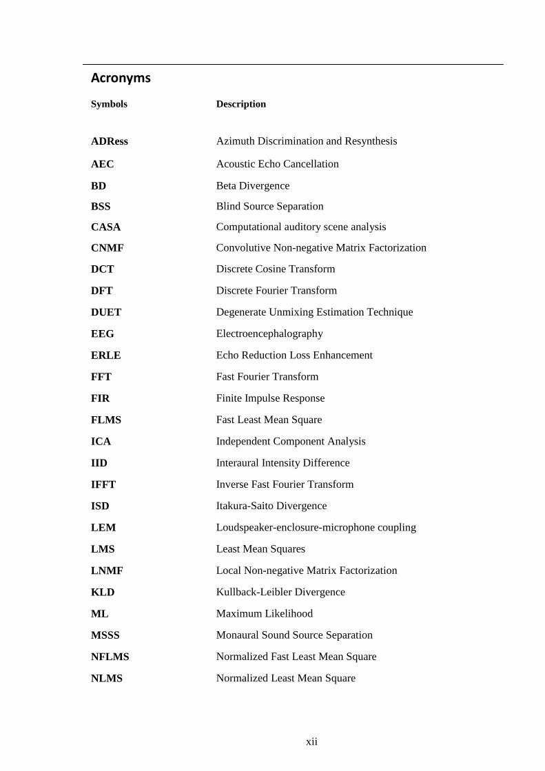
Acronyms

Symbols

Description

ADRess Azimuth Discrimination and Resynthesis

AEC Acoustic Echo Cancellation

BD Beta Divergence

BSS Blind Source Separation

CASA Computational auditory scene analysis

CNMF Convolutive Non-negative Matrix Factorization

DCT Discrete Cosine Transform

DFT Discrete Fourier Transform

DUET Degenerate Unmixing Estimation Technique

EEG Electroencephalography

ERLE Echo Reduction Loss Enhancement

FFT Fast Fourier Transform

FIR Finite Impulse Response

FLMS Fast Least Mean Square

ICA Independent Component Analysis

IID Interaural Intensity Difference

IFFT Inverse Fast Fourier Transform

ISD Itakura-Saito Divergence

LEM Loudspeaker-enclosure-microphone coupling

LMS Least Mean Squares

LNMF Local Non-negative Matrix Factorization

KLD Kullback-Leibler Divergence

ML Maximum Likelihood

MSSS Monaural Sound Source Separation

NFLMS Normalized Fast Least Mean Square

NLMS Normalized Least Mean Square

xiii

NMF Non-negative Matrix Factorization

PCA Principal Component Analysis

RIR Relative Incremental Reactivity

SAR Signal to Artifacts Ratio

SED Squared Euclidean Distance

SDR Signal to Distortion Ratio

SIR Signal to Interference Ratio

SNMF Sparse Non-negative Matrix Factorization

STFT Short Time Fourier Transform

TI Texas Instruments

VoIP Voice over Internet Protocol

1

Optimal Algorithms for Blind Source Separation -Application to Acoustic Echo Cancellation

1. Introduction

This thesis will address some of the aims of signal processing and machine learning

techniques, including extracting an interesting knowledge from experimental raw

datasets. In particular, we focus on the techniques related to blind source separation

(BSS) to solve one of its applications: Acoustic echo cancellation (AEC). The purpose

of this project focuses on finding a high quality and efficient technique to perform AEC.

Furthermore, to address the issue of sound dataset structure, we explore a recent

iterative technique called Non negative Matrix Factorization (NMF) [Daniel 01], also

we place particular emphasis on the initialization of current NMF algorithms for

efficiently computing NMF.

An aforementioned research area is blind source separation method. The sources

separation problems arise when a number of sources emit signals that mix and

propagate to one or more sensors. The objective is to identify the underlying source

signals based on measurements of the mixed sources. We have studied the feasibility of

various source separation techniques such as Independent Component Analysis (ICA),

Principal Component Analysis (PCA), and Degenerate Unmixing Estimation Technique

(DUET). In this thesis, we use both different types of LMS algorithms and

Non-negative Matrix Factorization (NMF) model to derive and implement in MATLAB,

using efficient and relatively simple iterative algorithms that work well in practice for

real-world data. Finally, we present an echo effect and echo control experiment on

real-time DSP board Texas Instruments Develop Start Kits (TMS320C6713 DSK) in

order to demonstrate a simple AEC solution.

1.1 Research problem description

This project aims to use different conventional mathematical techniques to perform

Acoustic Echo Cancellation. We will review the adaptive algorithms which are discussed

in later chapters and introduce a new optimal computational algorithm called NMF to

find the best suitable solution for AEC problem.

As the theory and applications of NMF is still being developed. In this project we choose

NMF algorithm to perform AEC using various divergence as a general cost function of

NMF, and find the optimal method that can give the best performance of AEC problem.

2


In addition, the workhorse in this project related NMF include initialization problem and

morphological constraints. These constrains include nonnegativity, sparsity,

orthogonality and smoothness. This research we also implement and optimize algorithm

for NMF and provide psedu-source code and efficient source code in MATLAB.

1.2 Thesis organization and overview

The focus of this thesis is the Acoustic Echo Cancellation using widely used adaptive

algorithm LMS and sound separation technique – NMF. Special emphasis is provided

coverage of the models and algorithms for nonnegative matrix factorizations both from

a theoretical and practical point of view. The main objective is to derive and implement

in MATLAB simulation. Actually, almost all of the experiments presented in this thesis

have been implemented in MATLAB and extensively tested. The layout of the thesis is

as follows.

In chapter two we provide the necessary background information and theory in sound

source separation and includes the different BSS generative mixing model. . In addition,

we also discuss the general principle of acoustic echo cancellation. It is main

application we have it involved in this project. And, we introduce the optimum solution

for the conversional acoustic echo canceller limitation at the end of this chapter.

In chapter three we discuss the blind source separation (BSS) and related methods

which present various optimization techniques and statistical methods to derive efficient

and robust learning or update rules. We present the conventional optimize algorithms

(i.e. ICA, PCA, DUET ADRess). This section discussed using different mathematical

techniques to perform sound source separation.

In chapter four we introduce the learning algorithms for Nonnegative Matrix

Factorization (NMF) and its properties of a large family of generalized and flexible

divergences between two nonnegative sequences or matrices. This chapter puts

particular emphasis on discussing NMF numerical approaches and various useful cost

functions and regulations of NMF, including those based on generalized

Kullback-Leibler, Pearson and Neyman Chi-squared divergences etc. Many of these

measures belong to the class of Alpha-divergences and Beta-divergences. In addition,

3


we give novel experiments on acoustic echo cancellation using extended NMF

algorithms.

In chapter five, two MATLAB simulation experiments present the requirements for

implementing the algorithms discussed in chapter three and four, and the measurements

that used to examine the output speech quality. We focus on Non-negative Matrix

Factorization algorithm implementation. Also the main contribution of this work is the

development a version of the NMF algorithm that combined the BSS principle,

represented the best route for tacking the AEC problem.

In chapter six, we extended the AEC problem on real-time implementation, and

demonstrated a simple straightforward echo control experiment based on TI C6713 DSP

start kits.

Chapter seven then contains conclusion on the work done and also highlights areas for

the future research in the area of NMF algorithm for blind source separation.

4


2. Acoustic Blind Source Separation background and theory

What is the blind source separation? The technique for estimation of individual source

components from their mixtures at multiple sensors is known as blind source separation

(BSS). In a real room environment, one well known BSS application is the separation of

audio sources which have been mixed and then captured by multiple sensors or

microphones. These sources could be different output signals from speakers in the same

room. Therefore, each sensor acquires a slightly different mixture of the original source

signals. One of the examples is solving the cocktail party problem [Bronkhorst 00]; we

will discuss it in chapter two. The term “blind” stresses the fact that the original source

signals and the generic mixing system are assumed to be unknown. Additionally, the

estimation is performed blindly, in other words, if the sources are to be separated blindly,

they should have some distinct characteristics, such as nonstationarity, non- Gaussianity.

One optimal learning algorithm: Independent component analysis (ICA) can calculate the

separation matrix, which is sometimes regarded as synonymous with BSS, relies on non-

Gaussianity [Lee 98][ Haykin 00][ Hyvärinen 01].

Furthermore, the fundamental assumption necessary for applying blind source separation

methods is that the original source signals are mutually statistically independent. The

fundamental problem of BSS refers to finding a demixing system whose outputs are

statistically independent. We will explain in detail the different mixture and separation

models for which most early BSS algorithms were designed in this chapter.

2.1 BSS Generative Model

One of the difficulties of the blind source separation task more particularly rely on the

way in which the signals are mixed within the physical environment. The simplest mixing

scenario deals with an instantaneous mixing model, for where no delayed versions of the

sources signals appear. This is the ideal case for which most early BSS algorithms were

designed, but such algorithms have limited practical applicability in real time speech

separation problems. In real world acoustical paths lead to convolutive mixing of the

sources when measured at acoustic sensors. It is an extension of the instantaneous mixing

model by considering also delayed versions of the source signals leading to a mixing

system. The system generally can be modelled by finite impulse response (FIR) filters.

5


When measuring the convolutive mixing of the sources, the degree of mixing is

significant since the reverberation time of the room space is large.

2.1.1 Instantaneous mixture model

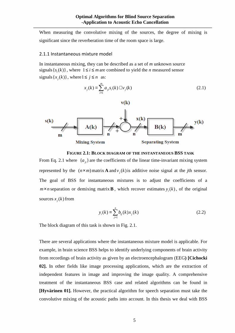
In instantaneous mixing, they can be described as a set of m unknown source signals{ ( )}is k , where 1 i m≤ ≤ are combined to yield the n measured sensor

signals{ ( )}jx k , where1 j n≤ ≤ as:

1

( ) ( ) ( )m

j ji i ji

x k a s k v k=

= +∑ (2.1)

FIGURE 2.1: BLOCK DIAGRAM OF THE INSTANTANEOUS BSS TASK

From Eq. 2.1 where { }jia are the coefficients of the linear time-invariant mixing system

represented by the ( )n m× matrixA and ( )jv k is additive noise signal at the jth sensor.

The goal of BSS for instantaneous mixtures is to adjust the coefficients of a

m n× separation or demixing matrixB , which recover estimates( )iy k , of the original

sources ( )jx k from

1

( ) ( ) ( )n

i ij jj

y k b k x k=

=∑ (2.2)

The block diagram of this task is shown in Fig. 2.1.

There are several applications where the instantaneous mixture model is applicable. For

example, in brain science BSS helps to identify underlying components of brain activity

from recordings of brain activity as given by an electroencephalogram (EEG) [Cichocki

02]. In other fields like image processing applications, which are the extraction of

independent features in image and improving the image quality. A comprehensive

treatment of the instantaneous BSS case and related algorithms can be found in

[Hyvärinen 01]. However, the practical algorithm for speech separation must take the

convolutive mixing of the acoustic paths into account. In this thesis we deal with BSS

6


for acoustic environments and thus the instantaneous mixture model is not appropriate

as no delayed versions of the source signals are considered. Therefore, in the next

section we extend this model and show how the convolutive mixture model works in

practical acoustic scenario.

2.1.2 Convolutive mixture model

In acoustic scenario, we extend the instantaneous mixture model by considering the

time delays resulting from sound propagation over space and probably the multipath

generated by reflections of sound off different objects, particularly in large rooms and

other enclosed settings. Normally, the convolutive mixing system consists of finite

impulse response filters. As a result, the m sources are mixed by a time-dispersive

multichannel system , described by

1

( ) ( ) ( )m

j jil i jl i

x k a s k l v k∞

=−∞ == − +∑∑ (2.3)

where{ ( )}jx k ,1 j n≤ ≤ are the n sensor signals. The parameter m also denotes the FIR

filter length of the demixing filter jila or we call the coefficients of the discrete-time

linear time-invariant mixing system{ }l l∞=−∞A , where each matrix lA is of

dimension( )n m× .

FIGURE 2.2: BLOCK DIAGRAM OF THE CONVOLUTIVE BSS TASK

In the above diagram, ( ) lll

z z∞ −=−∞

=∑A A and ( , ) ( ) lll

z k k z∞ −=−∞

=∑B B represent the z

transform of the sequences of the system{ }lA and{ ( )}l kB .

Most commonly, BSS algorithms are developed under the assumption that the number

m of simultaneously active source signal( )is k equals the number n of the sensor

7


signals ( )jx k . The number of unknown source signals m plays an important role in BSS

algorithms in that, under reasonable constraints on the mixing system, the separation

problem remains linear if the number of mixture signals n is greater than or equal to

m( )n m≥ . This case that the sensors outnumber the sources is termed overdetermined

BSS. The main approach to simplify the separation problem in this case is to apply

principal component analysis (PCA) [Hyvärinen 01]. In order to perform matrix

dimension reduction by extracting the first m components and then use a standard BSS

algorithm. A situation is called underdetermined BSS or BSS with overcomplete bases,

which means that the sources outnumber the sensors( )n m≤ . This is the significantly

more difficult case. Mostly the sparseness of the sources in the time-frequency domain

is used to determine clusters which correspond to the separated sources (e.g.

[Zibulevsky 01] [Bofill 03]. Currently, many researchers proposed methods to estimate

the sparseness of the sources based on modelling the human auditory system and then

subsequently apply time-frequency masking to separate the sources.

2.2 Speech source signal characteristics and BSS criteria

In this section we are going to discuss the signal properties of acoustic source signals

such as speech signals and their relevant utilization for BSS algorithms.

As we know, speech signals are feature-rich and possess certain characteristics that

enable BSS algorithm to be applied.

2.2.1 Basic signal properties of acoustic signals

Statistical properties: a good statistical model of a signal in the time domain is a

zero-mean Gaussian process ( , )N Nµ σℕ with a given variation 2Nσ , mean 0Nµ = and

normal probability density function (PDF) given by:

2

2

1( / , ) exp

22N N

NN

xp x µ σ

σσ π

= −

(2.4)

In the discrete time domain this simple model means that every sample has a random

value with a Gaussian PDF, also called Gaussian noise or Gaussian distribution.

Temporal properties: one of the widely used temporal properties of a noise signal is the

assumption that the noise is a stationary signal. In most cases in this thesis this is a

8


human speech signal. In other words, it is called “temporal dependencies” which means

audio signals are in general showing temporal dependencies, for example, the speech

signals by the vocal tract. Speech can also be separated using second-order statistics

alone if the source signals have unique temporal structures with distinct autocorrelation

functions. In other words, if the temporal sample of a signal is uncorrelated, then the

signal exhibits strict-sense whiteness.

Stationarity: speech is also a highly non-stationary signal due to the amplitude

modulations inherent in the voiced portions of speech and to the intermingling of voiced

and unvoiced speech patterns in most dialects [Scott 07]. The non-stationary

characteristics of individual talks (sources) are not likely to be similar. The majority of

audio signals are considered in literature as non-stationary signals, but strict-sense

stationarity is only assumed.

2.2.2 Criteria for BSS in Speech Separation

• Nonstationarity. BSS algorithms can be designed to exploit the statistical

independence of different talkers in an acoustic environment. It is known that

the statistic of jointly-Gaussian random processes can be completely specified

by their first or second order statistic; hence, the higher and lower order

statistical features do not carry any additional information about Gaussian

signals. Therefore, in most acoustic BSS applications nonstationarity of the

source signals can be exploited by simultaneous diagonalization of short-term

output correlation matrices at different time instants [Weinstein 93].

• Non-Gaussianity, in such case, statistical independence of the individual talker’s

signals need not be assumed, and the non-Gaussian nature of the speech signals

are not very important when these statistics are used. Additionally, the

non-gaussianity can be exploited by using higher-order statistics yielding a

statistical decoupling of higher-order joint moment of the BSS output signals.

BSS algorithms utilizing higher-order statistics are also termed independent

component analysis (ICA) algorithm [Cardoso 89][Jutten 91][Comon 91].

• Non-whiteness. As audio signals exhibit temporal dependencies this can be

exploited by the BSS criterion. Therefore, it can be assumed that samples of

each source signal are not independent along the time axis however; the signal

9


samples from different sources are mutually independent. Based on the

assumption of mutual statistical independence for non-white sources several

algorithms can be found in the literature. Mainly the non-whiteness is exploited

using second-order statistics by simultaneous diagonalization of output

correlation matrices over multiple time-lags. It notes that convolution based BSS

algorithm which is based on the mutual statistical independence for temporally

white signals.

2.3 Acoustic echo cancellation

2.3.1 General Principle

The effect of sound reflection from objects is called “reverberation.” Echoes are distinct

copies of the reflected sound. Humans can hear echoes when the difference between

arrival times of the direct signal and the reflection is more than 100ms, but even with

differences of 50ms the audio still sounds echoic. Most acoustic echo reduction

applications do not supress the echoes in the room environment, however, it actually

supresses the effect when the local sound source is captured by the receive device such

as microphone, transmitted through the communication line, reproduced by the

loudspeaker in the receiving room, captured by the microphone there, returned back

through the communication line, reproduced from the local loudspeaker, and so on. That

is the simple entire system converts to a signal generator, reproducing an annoying

constant one.

In addition, acoustic echo is inevitable whenever a speaker is placed near to a microphone

in a general full-duplex communication application. The most common communication

scenario is the hands-free mobile communication kits for the cars. For example, the voice

from the loudspeaker is unavoidable to be picked up by the microphone and transmitted

back to the remote speaker. This makes the remote speaker hear his/her own voice

distorted and delayed by the communication channel or called end to end delay, which is

known as echo. Obviously, the longer the channel delay, the more annoying the echo

and the worse is the perceived quality of the communication service such as VoIP

conference call.

There are some properties of acoustic echo:

10


� It is not stationary, and is varies based on a multitude of external factors –

intensity and position of the sound source.

� It is a non-linear signal; the non-linearity might be created by the analogue

circuitry.

� It is more dispersive, with dispersion times up to 100ms.

2.3.2 Joint Blind Source Separation and Echo Cancellation

2.3.2.1 Cause of Echo in digital network

In most situations, background noise is generated through the network when we use

digital phones operated in hands-free mode. In the real-time environment, the additional

sounds are directly and indirectly transmitted to the microphone, so the multipath audio is

created and transmitted back to the talker. These additional sounds pass through the

digital cellular vocoder and cause distortion of speech. Meanwhile, the digital processing

delays and speech-compression applied further contribution of the echo generation and

degraded voice quality.

Under this circumstance, the echo-control systems are required in today’s digital wireless

networks. Because of the speech process delays ranging from 80ms to 100ms are

introduced, and then resulting in total end-to-end delay of approximately 160ms to

200ms. At this stage, the echo cancellation devices are required within the wireless

network.

There are two main echo cancellation types: line echo cancelation and acoustic

cancellation. General speaking, line echo is created by a telephone hybrid which

transforms a 4 wire line to a 2 wire line. Usually there are two hybrids in the telephone

line. One corresponds to the near end terminal and the other one corresponds to the far

end (remote) terminal. See the figure 2.3 for the line echo flow diagram.

11


FIGURE 2.3: L INE ECHO CANCELLER INTEGRATION FLOW DIAGRAM Line echo canceller features include: fast convergence, fast re-convergence after echo

path change, robustness in respect to background noise and non-linear distortion,

maximal echo path up to 256ms, reliable work in networks with VoIP segments.

Additionally, acoustic echo cancellation compares with line echo cancellation, both of

them address the similar problems, and are often based on the same technology.

However, a line echo canceller generally cannot replace an acoustic echo canceller; due

to acoustic echo cancellation is a more difficult problem. With line echo cancellation

there are generally less than two reflections from telephone hybrids or impedance

mismatches in the telephone line. These echoes are usually delayed by less than 32 ms,

and do not change very frequently. As mentioned before, with acoustic echo

cancellation, the echo path is complex and also varies continuously as the speaker

moves around the room.

2.3.2.2 The Process of Echo Cancellation and performance measurement

Today’s digital cellular network technologies require significantly more processing

power to transmit signals through the channels.

Simply said, the process of cancelling echo involves two steps.

� Calling set up: the echo canceller employs a digital adaptive filter to set up a

model of voice signal and echo passing through the echo canceller. As a voice

path passes back through the cancellation system, the echo canceller compared

the original signal and “modelled” signal to cancel existing echo dynamically.

12


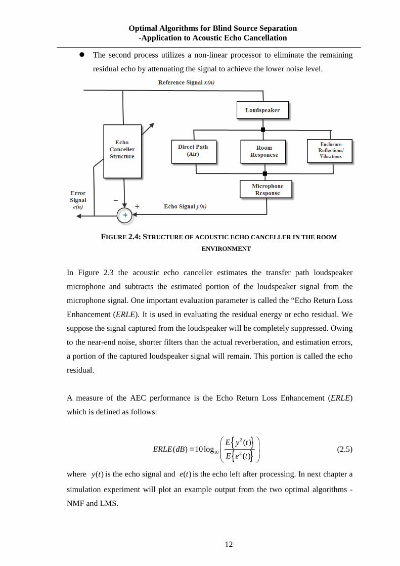
� The second process utilizes a non-linear processor to eliminate the remaining

residual echo by attenuating the signal to achieve the lower noise level.

FIGURE 2.4: STRUCTURE OF ACOUSTIC ECHO CANCELLER IN THE ROOM

ENVIRONMENT

In Figure 2.3 the acoustic echo canceller estimates the transfer path loudspeaker

microphone and subtracts the estimated portion of the loudspeaker signal from the

microphone signal. One important evaluation parameter is called the “Echo Return Loss

Enhancement (ERLE). It is used in evaluating the residual energy or echo residual. We

suppose the signal captured from the loudspeaker will be completely suppressed. Owing

to the near-end noise, shorter filters than the actual reverberation, and estimation errors,

a portion of the captured loudspeaker signal will remain. This portion is called the echo

residual.

A measure of the AEC performance is the Echo Return Loss Enhancement (ERLE)

which is defined as follows:

{ }{ }

2

10 2

( )( ) 10 log

( )

E y tERLE dB

E e t

=

(2.5)

where ( )y t is the echo signal and ( )e t is the echo left after processing. In next chapter a

simulation experiment will plot an example output from the two optimal algorithms -

NMF and LMS.

13


2.3.2.3 AEC applications with BSS algorithm

In some applications such as teleconferencing and voiced-controlled machinery, AEC has

been widely used in this kind of real applications. However, this straightforward

approach would be to use multichannel AEC which has two important drawbacks:

� The AEC can only operate reliably when one of the speakers are talking; it means it

will not work properly when there is double talk. As louder speakers to microphone

fast adaptation is required which cannot be obtained in the presence of double talk.

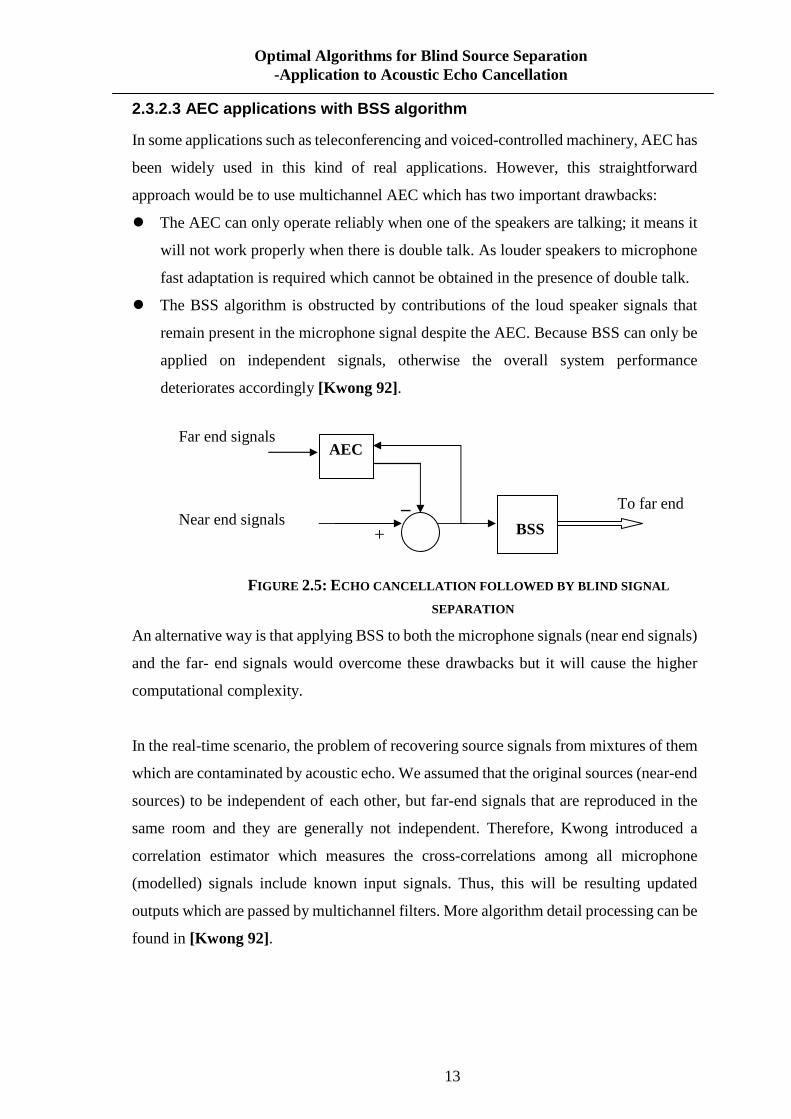
� The BSS algorithm is obstructed by contributions of the loud speaker signals that

remain present in the microphone signal despite the AEC. Because BSS can only be

applied on independent signals, otherwise the overall system performance

deteriorates accordingly [Kwong 92].

An alternative way is that applying BSS to both the microphone signals (near end signals)

and the far- end signals would overcome these drawbacks but it will cause the higher

computational complexity.

In the real-time scenario, the problem of recovering source signals from mixtures of them

which are contaminated by acoustic echo. We assumed that the original sources (near-end

sources) to be independent of each other, but far-end signals that are reproduced in the

same room and they are generally not independent. Therefore, Kwong introduced a

correlation estimator which measures the cross-correlations among all microphone

(modelled) signals include known input signals. Thus, this will be resulting updated

outputs which are passed by multichannel filters. More algorithm detail processing can be

found in [Kwong 92].

Far end signals

_ To far end Near end signals

+

FIGURE 2.5: ECHO CANCELLATION FOLLOWED BY BLIND SIGNAL

SEPARATION

AEC

BSS

14


The above example is taking advantage of BSS algorithm over conventional echo

cancellation is that can operate in many suitable applications such as teleconferencing

and hands free telephony.

2.3.3 Limitation of conventional Acoustic Echo Canceller

Much work has be carried out aimed at [Kwong 92][Makino 93][Mathews 93]

improving the convergence speed of LMS type algorithm. Ideally, an acoustic echo

canceller is to completely remove any signal emanating from a loudspeaker from the

signal picked up by a closely coupled microphone. In short conclusion of limitations of

echo cancellers for speakerphones includes:

• Acoustic, thermal and DSP related noise

• Inaccurate modelling of the room impulse response

• Slow convergence and dynamic tracking

• Nonlinearities in the transfer function caused mainly due to the loudspeaker

• Resonances and vibration in the plastic enclosure.

To be commercially viable the AEC needs to be developed in products for a

self-contained handsfree device in a typical room environment. An important part of the

acoustic each canceller evaluation is the convergence time and it is necessary to be set

on the order of 100ms with Echo Return Loss Enhancement (ERLE) on the order of

30dB.

2.3.4 Conclusions

Acoustic echo cancellation is useful in any hands-free or other telecommunications

situation involving two or more locations. Acoustic echo is most noticeable and

annoying when delay is present in the transmission path. This would happen primarily

in long distance circuits, or systems utilizing speech compression such as VoIP

application. However the echo might not be as annoying when there is no delay (e.g.

with short links between conference rooms in the same building or distance learning

over high speed fibre-optic cable connection. As the existence of imperfection of speech

quality in the modern telecommunication, acoustic echo cancellation techniques will

have large commercial potential in the future.

15


3 Optimum Algorithms for Blind Source Separation

3.1 Independent Component Analysis (ICA)

3.1.1 Background Theory of Independent Component Analysis

Blind source separation (BSS) is the problem of recovering signals from several observed

linear mixtures. These signals could be from different directions or they could have

different pitch levels along the same directions. When we deal with the BSS, there is no

need for information on the source signals or mixing system (location or room acoustics)

[Makino 07a]. Here, we should point out that the characteristics of the source signals are

statistically independent, as well as independent from the noise components. Therefore

the goal of BSS is to separate an instantaneous linear even-determined mixture of

non-Gaussian independent sources [Paul 05].

As we mix independent components (random independent variables) the resulting mix

tends towards having a Gaussian distribution, making the Independent Components

Analysis (ICA) method impossible. ICA is the classical blind source separation method to

deal with problems that are closely related to the cocktail-party problem. The following

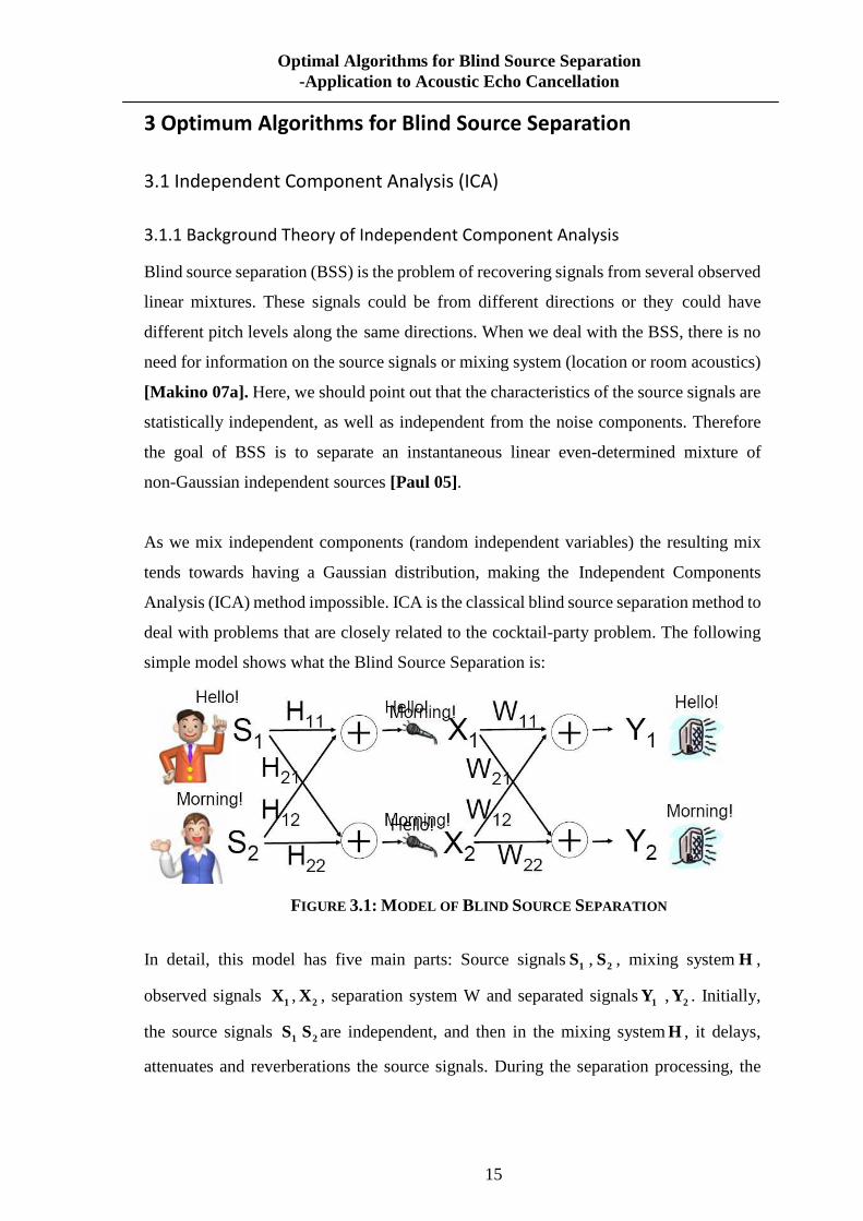
simple model shows what the Blind Source Separation is:

FIGURE 3.1: MODEL OF BLIND SOURCE SEPARATION

In detail, this model has five main parts: Source signals 1S , 2S , mixing systemH ,

observed signals 1X , 2X , separation system W and separated signals1Y , 2Y . Initially,

the source signals 1S 2S are independent, and then in the mixing systemH , it delays,

attenuates and reverberations the source signals. During the separation processing, the

16


separation systemW only uses the observed signals1X , 2X to estimate 1S , 2S . The

separated signals1Y , 2Y should become mutually independent.

Ideally, the aim of the source separation is not necessarily to recover the originally source

signal. Instead, the aim is to recover the model sources without interferences from the

other source. Therefore, each model source signal can be a filtered version of the original

source signals.

3.1.2 Notation of Blind Source Separation

In the Blind Source Separation problem, for example, m mixed signals are linear

combinations of n unknown mutually statistically, independent, zero-mean source signal,

and are noise-contaminated source signals. So this is can be written as:

1

( ) ( ) ( ) 1...n

i ij j ij

x t h s t n t i m=

= + =∑ (3.1)

Its matrix notation:

X(t) = HS(t) + N(t) (3.2)

Where T1 2 mX(t) = [x (t), x (t), ..., x (t)] , is a vector of sensor signals, N(k) is the vector of

additive noise. H is the unknown full rank n m× mixing matrix. The block diagram as

shown below:

FIGURE 3.2: BLOCK DIAGRAMS ILLUSTRATING BLIND SIGNAL PROCESSING PROBLEM We consider equation (3.1) as a linear function in most cases, and every component

( )ix t is expressed as a linear combination of the observed variables ( )js t .

17


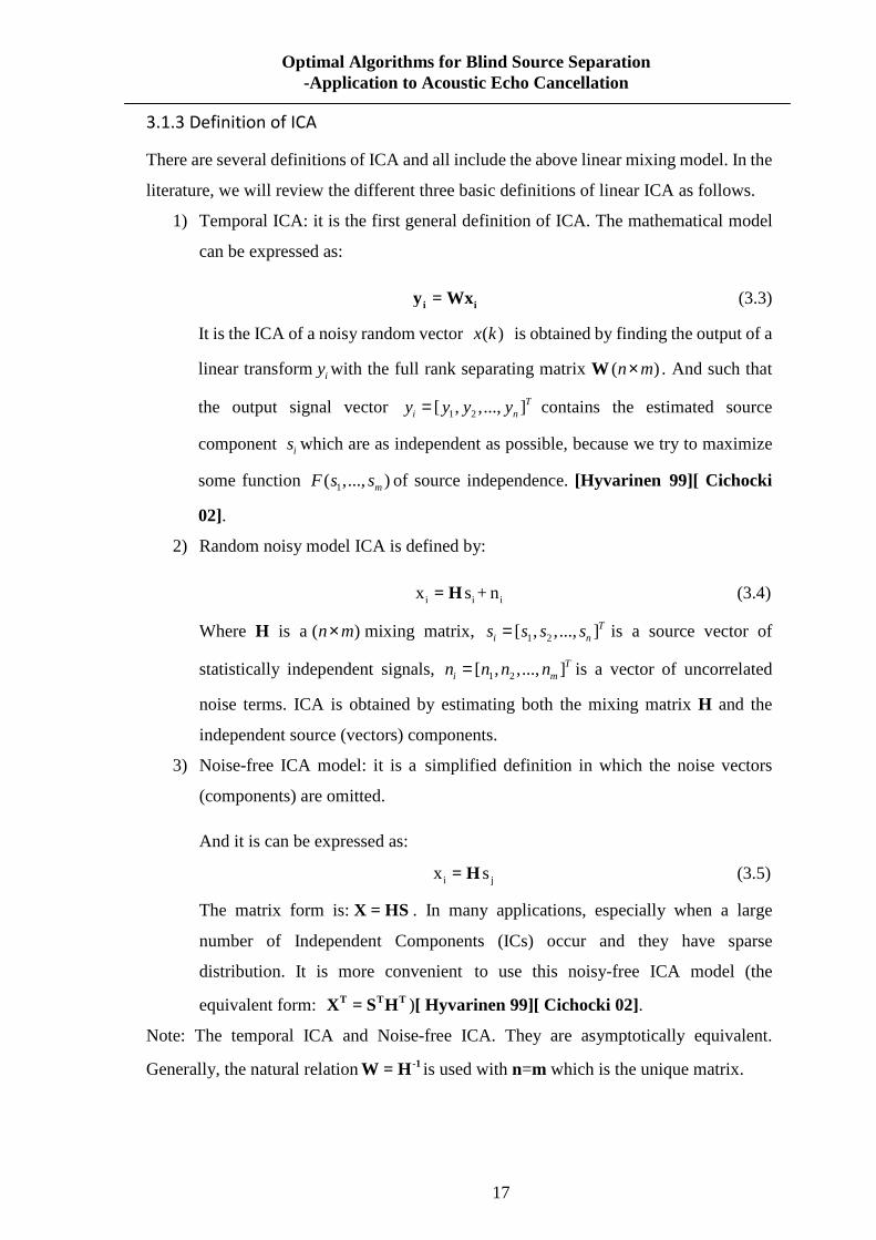
3.1.3 Definition of ICA

There are several definitions of ICA and all include the above linear mixing model. In the

literature, we will review the different three basic definitions of linear ICA as follows.

1) Temporal ICA: it is the first general definition of ICA. The mathematical model

can be expressed as:

i iy = Wx (3.3)

It is the ICA of a noisy random vector ( )x k is obtained by finding the output of a

linear transform iy with the full rank separating matrix W ( )n m× . And such that

the output signal vector 1 2[ , ,..., ]Ti ny y y y= contains the estimated source

component is which are as independent as possible, because we try to maximize

some function 1( ,..., )mF s s of source independence. [Hyvarinen 99][ Cichocki

02].

2) Random noisy model ICA is defined by:

i i ix s + n= H (3.4)

Where H is a( )n m× mixing matrix, 1 2[ , ,..., ]Ti ns s s s= is a source vector of

statistically independent signals, 1 2[ , ,..., ]Ti mn n n n= is a vector of uncorrelated

noise terms. ICA is obtained by estimating both the mixing matrix H and the

independent source (vectors) components.

3) Noise-free ICA model: it is a simplified definition in which the noise vectors

(components) are omitted.

And it is can be expressed as:

i jx s= H (3.5)

The matrix form is:X = HS . In many applications, especially when a large

number of Independent Components (ICs) occur and they have sparse

distribution. It is more convenient to use this noisy-free ICA model (the

equivalent form: T T TX = S H )[ Hyvarinen 99][ Cichocki 02].

Note: The temporal ICA and Noise-free ICA. They are asymptotically equivalent.

Generally, the natural relation -1W = H is used with n=m which is the unique matrix.

18


From the definition 3, the basic noisy-free ICA model is a generative model [Hyvarinen

99b], which means that it describes how the observed data are generated by a process of

mixing the components js (sources), and these components are latent variables, meaning

that they cannot be directly observed. All we observe are the random variablesix , and we

must estimate both the mixing coefficientsH , and the ICs is (estimated sources) usingix .

Here we have dropped the time index t and this is because in the basic ICA model, we

assume that each mixture ix as well as each independent component js (sources) is a

random variable, instead of a proper time signal or time series. We also neglect any time

delays during the mixing. So this is often called the instantaneous mixing model.

3.1.4 Restrictions in ICA

There are three certain assumptions and restrictions to make sure the basic ICA model can

be estimated.

1) The independent components are assumed statistically independent.

The random variables are said to be independent if the source componentis does

not give any information on the value of another source component js for i j≠ .

Technically, the independence can be defined by the probability densities.

(Note: more details relate joint pdf and marginal pdf, see section 2.3 on ICA

[Hyvarinen 99c])

2) The independent components must have Non-Gaussian distributions.

The Gaussian components mix the independent components and cannot be

separated from each other. In other words, some of the estimated components will

be arbitrary linear combinations of the Gaussian components and in the

Non-Gaussian distributions we can find the independent components. Thus, ICA

is essentially impossible if the observed mixtures ix (variables) have Gaussian

distributions.

3) We can assume that the unknown, mixing matrix is square.

This assumption means, the number of independent components is is equal to

the number of observed mixtureix . This simplifies the estimation (from original

source) very much.

19


3.1.5 Background theory of ICA

There are three basic and intuitive principles for estimating the model of independent

component analysis.

1) ICA by minimization of mutual information.

There is a basic definition of information-theoretic concepts explained in this

section.

The differential entropyH of a random vector y with density p(y) is defined as

[Hyvarinen 99c]:

( ) ( ) log ( )H y p y p y dy= −∫ (3.6)

The entropy is closely related to the code length of the random vector. Basically,

the mutual informationI between m (scalar) random variables , 1....iy i m= is

defined as follows:

1 21

( , ,..., ) ( ) ( )m

m ii

y y y y y=

= −∑I H H (3.7)

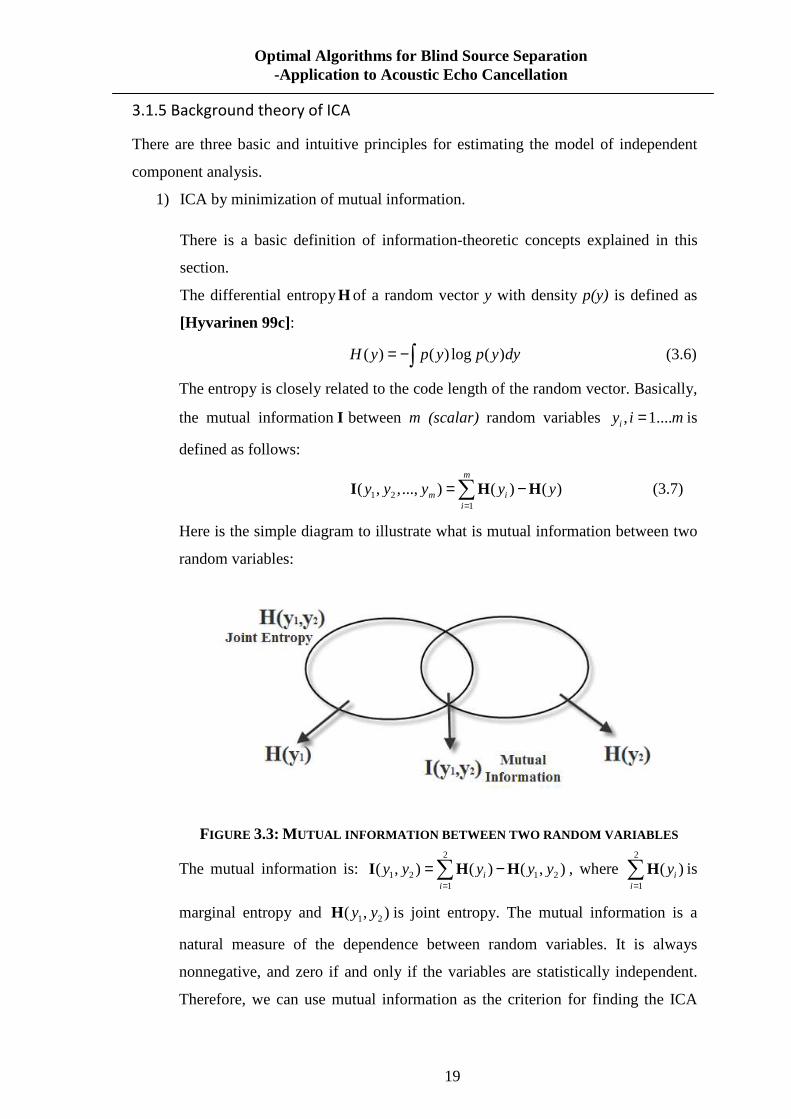
Here is the simple diagram to illustrate what is mutual information between two

random variables:

FIGURE 3.3: MUTUAL INFORMATION BETWEEN TWO RANDOM VARIABLES

The mutual information is: 2

1 2 1 21

( , ) ( ) ( , )ii

y y y y y=

= −∑I H H , where 2

1

( )ii

y=∑H is

marginal entropy and 1 2( , )y yH is joint entropy. The mutual information is a

natural measure of the dependence between random variables. It is always

nonnegative, and zero if and only if the variables are statistically independent.

Therefore, we can use mutual information as the criterion for finding the ICA

20


representation, i.e. to make the output “decorrelated”. In any case, minimization

of mutual information can be interpreted as giving the maximally independent

components [Hyvarinen 99c].

2) ICA by maximization of Non-Gaussianity.

Non-Gaussianity is actually most important in ICA estimation. In classic

statistical theory, random variables are assumed to have Gaussian distributions.

So we start by motivating the maximization of Non-Gaussianity by the central

limit theorem. It has important consequences in independent component analysis

and blind source separation. As mentioned in the first section, a typical mixture of

the random data vectorx , is of the form1

m

i ij jj

a=

=∑x s , where , 1,....,ija j m= , are

constant mixing coefficients and, 1,...,j j m=s , are the m unknown source signals.

Even for a small number of sources the distribution of the mixture is usually close

to Gaussian.

Simply explained as follows:

Let us assume that the data vector x is distributed according to the ICA data

model:x s= H , it is a mixture of independent components. Estimating the

independent components can be accomplished by finding the right linear

combinations of the mixture variables. We can invert the mixing model as:

-1s = H x , so the linear combination is ix . In other words, we can denote this by

.∑Ti i

i=1

y = b x = b x We could take b as a vector that maximizes the

Non-Gaussianity ofTb x . This means that Ty = b x equals one of the independent

components. Therefore, maximizing the Non-Gaussianity of Tb x gives us one of

the independent components. [Hyvarinen 99c] To find several independent

components, we need to find all these local maxima. This is not difficult, because

the different independent components are uncorrelated: We can always constrain

the search to the space that gives estimates uncorrelated with the previous ones.

[Hyvarrinen 04]

3) ICA by maximization of likelihood.

Maximization of likelihood is one of the popular approaches to estimate the

independent components analysis model. Maximum likelihood (ML) estimator

21


assumes that the unknown parameters are constants if there is no prior

information available on them. It usually applies to large numbers of samples.

One interpretation of ML estimation is calculating parameter values as estimates

that give the highest probability for the observations.

There are two algorithms to perform the maximum likelihood estimation:

• Gradient algorithm: this is the algorithms for maximizing likelihood

obtained by the gradient method. (Further Ref. See [Hyvarinen 99d])

• Fast fixed-point algorithm [Ella 00]: the basic principle is to maximize the

measures of Non-Gaussianity used for ICA estimation. Actually, the

FastICA algorithm (gradient-based algorithm but converge very fast and

reliably) can be directly applied to maximization of the likelihood.

3.2 Principal Component Analysis (PCA)

3.2.1 Introduction

Principal Component Analysis is one of the simplest and better known data analysis

techniques. The main purpose of PCA analytic techniques are: a) to reduce the number of

variables. b) to detect structure in the relationships between variables, that is to classify

variables. In other words, PCA is combining two or more variables into a single factor

where these variables might be highly correlated with each other.

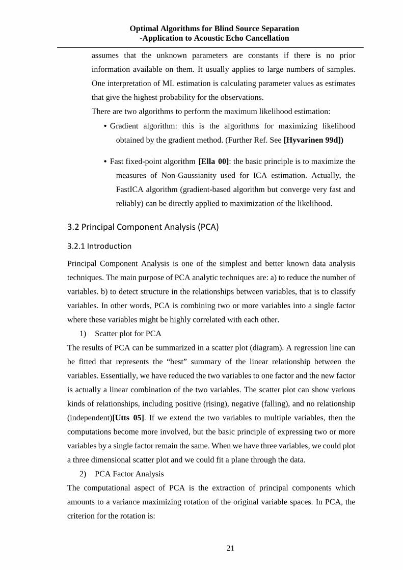
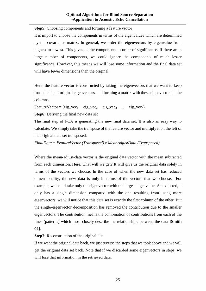
1) Scatter plot for PCA

The results of PCA can be summarized in a scatter plot (diagram). A regression line can

be fitted that represents the “best” summary of the linear relationship between the

variables. Essentially, we have reduced the two variables to one factor and the new factor

is actually a linear combination of the two variables. The scatter plot can show various

kinds of relationships, including positive (rising), negative (falling), and no relationship

(independent)[Utts 05]. If we extend the two variables to multiple variables, then the

computations become more involved, but the basic principle of expressing two or more

variables by a single factor remain the same. When we have three variables, we could plot

a three dimensional scatter plot and we could fit a plane through the data.

2) PCA Factor Analysis

The computational aspect of PCA is the extraction of principal components which

amounts to a variance maximizing rotation of the original variable spaces. In PCA, the

criterion for the rotation is:

22


• Maximize the variance of the “new” variables (factor).

• Minimizing the variance around the new variable.

After the first regression line has been found through the data, we iteratively continue to

define other lines that maximize the remaining variability. In this manner, consecutive

factors are extracted and these factors are independent of each other. In other words,

consecutive factors are uncorrelated or orthogonal to each other [Dinov 04]. Note that the

decision of when to stop extracting factors basically depends on when there is only very

little random variability left. Also the variances extracted by the factor are called the

eigenvalues. As expected, the sum of the eigenvalues is equal to the number of variables.

We will discuss more about eigenvalues in the next section.

3.2.2 Mathematics Background

• Eigenvalue and Eigenvector

Calculating Eigenvalues and Eigenvectors is the key point in PCA. PCA involves

determining of these two parameters of the covariance matrix. We will talk in more detail

about the covariance matrix in the next section.

Eigenvalues are a special set of scalars associated with a linear system of equations that

are sometimes also known as characteristic roots. Each eigenvalue is paired with a

corresponding so-called eigenvector. The determination of the eigenvalues and

eigenvectors of a system is very important in engineering, where it is equivalent to matrix

diagonalization.

Matrix diagonalization is the process of taking a square matrix and converting it into a

so-called diagonal matrix that shares the same fundamental properties of the underlying

matrix. The relationship between a diagonalized matrix, eigenvalues, and eigenvectors

follows from the great mathematical identity. For example, a square matrix A can be

decomposed into the very special form: 1−=A PDP , where P is a matrix composed of the

eigenvectors ofA ; D is the diagonal matrix constructed from the corresponding

eigenvalues, and the 1−P is the inverse matrix of P [George 97].

• Covariance

Firstly we need to understand what covariance is. The covariance of two datasets Cx,y (x

and y) can be defined as their tendency to vary together. We usually define these two

23


datasets as a two dimensional dataset. In statistics, the variability of the data set around its

mean is called the data standard deviation. In the same way, covariance can describe

variability—as the product of the averages of the deviation of the data points from the

mean value. There are three possible results which can indicate the relationship between

the two datasets.

Cx,y value will be larger than 0 (positive) if x and y tend to increase together.

Cx,y value will be less than 0 (negative) if x and y tend to decrease together.

Cx,y value will equal 0 if x and y are independent.

Since the covariance value can be calculated between any 2 dimensions in the data set,

this technique is often used to find relationships between dimensions in high-dimensional

data sets where visualisation is difficult.

Also measuring the covariance between x and y would give us the variance of the x, y

dimensions respectively. The formula for covariance is:

1( )( )

cov( , )1

n

i iix x y y

x yn

=− −

=−

∑ (3.8)

For each item, multiply the difference between the x value and the mean of x, by the

difference between the y value and the mean of y and add all these up, and divide by n-1.

• Covariance matrix

In fact, for an n-dimensional data, there are !

( 2)!*2

n

n− different covariance values.

Generally, a useful way to get all the possible covariance values between all the different

dimensions is to calculated them all and put them in a matrix. For example, for 2D data

the covariance matrix has two dimensions, and the values are this:

cov( , ) cov( , )

cov( , ) cov( , )

x x x y

y x y y

=

C (3.9)

Basically, if we have an n-dimensional data set, then the matrix has n rows and n columns

(must be square) and each entry in the matrix is the result of calculating the covariance

between two separate dimensions.

3.2.3 PCA Methodology

The dimension of the data is the number of variables that are measured on each

observation. A high dimensional dataset contains more information compared with a low

24


dimension counterpart. To reduce the dimensionality of the data while retaining as much

as possible of the variation present in the original dataset is the goal of PCA. In

mathematical terms, we can state this as follows:

Given the p-dimensional random variable 1( ,..., )Tpx x=x , find a lower dimensional

representation of it, 1( ,..., )Tks s=s withk p≤ , that captures the content in the original

data. But dimensionality reduction implies information loss; our task is to preserve as

much information as possible and determine the best lower dimensional space.

Technically, the best low-dimensional space can be determined by the “best”

eigenvectors of the covariance matrix of x (i.e. the “best” eigenvectors corresponding to

the “largest” eigenvalues – also called “principak components”) [Simth 02].

3.2.4 Procedure of PCA

Step1: Collect and prepare a set of data and obtain the mean value

Suppose 1 2, ,..., mx x x are 1m× vector, and mean is 1

1 m

ii

x xm =

= ∑

Step2: Subtract the mean value from each data element ( )( )x x y y− −

The mean subtracted is the average across each dimension and it produces a data set

whose mean is zero. So, all thex values have x subtracted, and y values have

y subtracted from them.

Step3: Calculate the covariance matrix

This is done in the same way as was discussed in the previous section.

Step4: Determine the eigenvalues and eigenvectors of the covariance matrix

Since the covariance matrix is square, we can calculate the eigenvalues and eigenvectors

for this matrix. It is important to tell us useful relationship information about the data –

increase, decrease together or independent. Each eigenvalue is a measure of how much

variance each successive factor extracts, and associated the eigenvector shows us how

these dataset are related along a regression line. The process of taking the eigenvector of

the covariance matrix, we have been able to extract lines that characterise the scatter of

the data.

25


Step5: Choosing components and forming a feature vector

It is import to choose the components in terms of the eigenvalues which are determined

by the covariance matrix. In general, we order the eigenvectors by eigenvalue from

highest to lowest. This gives us the components in order of significance. If there are a

large number of components, we could ignore the components of much lesser

significance. However, this means we will lose some information and the final data set

will have fewer dimensions than the original.

Here, the feature vector is constructed by taking the eigenvectors that we want to keep

from the list of original eigenvectors, and forming a matrix with these eigenvectors in the

columns.

FeatureVector = (eig_vec1 eig_vec2 eig_vec3 ... eig_vecn)

Step6: Deriving the final new data set

The final step of PCA is generating the new final data set. It is also an easy way to

calculate. We simply take the transpose of the feature vector and multiply it on the left of

the original data set transposed.

FinalData = FeatureVector (Transposed) x MeanAdjustData (Transposed)

Where the mean-adjust-data vector is the original data vector with the mean subtracted

from each dimension. Here, what will we get? It will give us the original data solely in

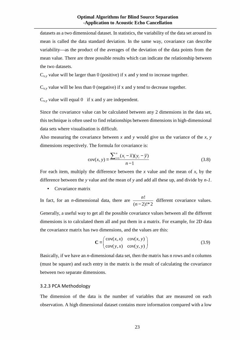
terms of the vectors we choose. In the case of when the new data set has reduced

dimensionality, the new data is only in terms of the vectors that we choose. For

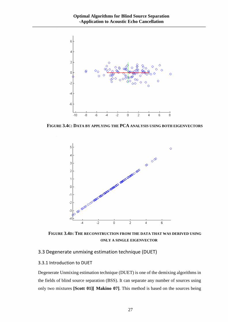
example, we could take only the eigenvector with the largest eigenvalue. As expected, it

only has a single dimension compared with the one resulting from using more

eigenvectors; we will notice that this data set is exactly the first column of the other. But

the single-eigenvector decomposition has removed the contribution due to the smaller

eigenvectors. The contribution means the combination of contributions from each of the

lines (patterns) which most closely describe the relationships between the data [Smith

02].

Step7: Reconstruction of the original data

If we want the original data back, we just reverse the steps that we took above and we will

get the original data set back. Note that if we discarded some eigenvectors in steps, we

will lose that information in the retrieved data.

26


TransDataAdjust = TransFeatureVector-1×FinalData

After calculating the adjusted data set, we need to add the mean to each dimension of the

data set to retrieve the original data set.

TransOriginalData = TransDataAdjust + OriginalMean

The following figure shows the essential procedure of PCA.

FIGURE 3.4A: ORIGINAL TWO DIMENSIONAL DATA

FIGURE 3.4B: NORMALIZED TWO DIMENSIONAL DATA

27


FIGURE 3.4C: DATA BY APPLYING THE PCA ANALYSIS USING BOTH EIGENVECTORS

FIGURE 3.4D: THE RECONSTRUCTION FROM THE DATA THAT WAS DERIVED USING

ONLY A SINGLE EIGENVECTOR

3.3 Degenerate unmixing estimation technique (DUET)

3.3.1 Introduction to DUET

Degenerate Unmixing estimation technique (DUET) is one of the demixing algorithms in

the fields of blind source separation (BSS). It can separate any number of sources using

only two mixtures [Scott 01][ Makino 07]. This method is based on the sources being

28


w-disjoint orthogonal. Common assumptions about the statistical properties of the

sources are statistically independent [Bell 05][Cardoso 97], are statistically orthogonal

[Weinstein 93], are nonstationary [Parra 00], or can be generated by finite dimensional

model spaces [Broman 99]. Moreover, the DUET algorithm is efficient for sources

having a property of sparseness in the time-frequency domain, such as speech signal, that

is, the target speech signal in a noisy environment can be effectively recognised using the

DUET algorithm for Blind Source Separation.

However, in many cases there are more sources than mixtures so we refer to such a case

as degenerate. In degenerate Blind Source Separation poses a challenge because the

mixing matrix is not invertible. Basically, the traditional method such as Independent

Component Analysis (ICA) of demixing by estimating the inverse mixing matrix does not

work. Therefore, most blind source separation research has focussed on the square or

non-degenerate case [Scott 01][ Makino 07]. Despite the difficulties, there are several

approaches for dealing with degenerate mixtures. We will review these approaches in

the next few sections.

Generally, DUET solves the degenerate demixing problem in an efficient and robust

manner. We can summarized in one sentence as a definition: DUET makes it possible to

blindly separate an arbitrary number of sources given just two anechoic mixtures provide

the time-frequency representations of the sources do not overlap too much, which is ideal

for speech [Makino 07].

3.3.2 Sources assumptions and mathematics background

• Anechoic Mixing

Consider the mixture of N source signals,( ), 1,...,t j N=js , being received at a pair of

microphones on a direct path. Suppose we can absorb the attenuation and delay

parameters of the first mixture (t)1x into the definition of the sources without loss of

generality. Then the two anechoic mixtures can be expressed as:

1

( ) ( ) N

j

t t=

=∑1 jx s (3.10)

1

( ) ( )N

j jj

t a t δ=

= −∑2 jx s (3.11)

Where ja is a relative attenuation factor corresponding to the ratio of the attenuations of

the paths between sources and sensors, jδ is the arrival delay between the sensors.

29


Actually the DUET method, which is based on the anechoic model is quite robust even

when applied to echoic mixtures.

• W-Disjoint Orthogonality

In mathematics, disjoint means if two or more sets are disjoint they have no element in

common, or say their intersection is the empty set.

W-disjoint orthogonality is crucial to DUET because it allows for the separation of a

mixture into its component sources using a binary mask. (Note: a binary mask is used to

change specific bits in the original value in the time-frequency plane to the desired

setting(s) or to create a specific output value).

We can call two functions ( )js t and ( )ks t W-disjoint orthogonal. For a given windowing

function ( )W t , the supports of the windowed Fourier transform of ( )js t and ( )ks t are

disjoint. The windowed Fourier transform of ( )js t is defined as:

1

ˆ ( , ) : ( ) ( )2

i tj js W t s t e dtωτ ω τ

π∞ −

−∞= −∫ (3.11)

We can state the W-disjoint orthogonality assumption concisely as the following

expression:

ˆ( , ) ( , ) 0, , , .j ks s j kτ ω τ ω τ ω= ∀ ∀ ≠ (3.12)

This assumption is a mathematical idealization of the condition (Note: Idealization is the

over-estimation of the desirable qualities and underestimation of the limitations of a

desired thing [Changing 00] .) In other words, it is likely that every time-frequency point

in the mixture with significant energy is dominated by the contribution of one source. In

this case, W-disjoint orthogonality can be expressed as,

ˆ( ) ( ) 0, , j ks s j kω ω ω= ∀ ∀ ≠ (3.13)

As mentioned before, the binary mask can be used to separate the mixture. So consider

the mask function for the support ofˆ js ,

ˆ0 ( , ) 0

( , ) :1 otherwise

jj

sM

τ ωτ ω

≠=

(3.14)

jM separates js from the mixture via

1ˆ ˆ( , ) ( , ) ( , ), ,j js M xτ ω τ ω τ ω τ ω= ∀ (3.15)

30


We must determine the masks which are the indicator functions ( , )jM τ ω for each

source and separate the sources by partitioning. The question is: how do we determine the

masks? We will review and discuss it shortly.

3.3.3 Local stationarity and Microphones close together

Local stationarity can be viewed as a form of narrowband assumption. It is necessary for

DUET that for all arrival delay timeδ , δ ≤ ∆ , where ∆ is the maximum time difference

possible in the mixing model (Maximum distance of two microphones divided by the

speed of signal propagation), even when the window function ( )W t has finite support.

Additionally, in the common array processing literature [Krim 96] , the physical

separation of the sensors is small such that the relative delay between the sensors can be

expressed as a phase shift of the signal.

We can utilize the local stationarity assumption to turn the delay in time into a

multiplicative factor in time-frequency. Basically, this multiplicative factor ie ωδ− only

uniquely specifies δ if ωδ π< as otherwise we have an ambiguity due to phase-wrap

[Makino 07b]. So we require, , , ,j jωδ π ω< ∀ ∀ avoiding phase ambiguity. Therefore,

this is guaranteed when two microphones are separated by less than

max/cπ ω where maxω is the maximum frequency present in the sources and c is the speed

of sound.

3.3.4 DUET demixing model and parameters

The assumptions of anechoic mixing and local stationarity allow us to rewrite the mixing

equations (1) and (2) in the time- frequency domain as,

1

11

2 1

ˆ ( , )11ˆ ( , ) ...

ˆ ( , ) ...ˆ ( , )

NiiN

N

sx

x a ea es

ωδωδ

τ ωτ ωτ ω

τ ω−−

=

⋮ (3.16)

This is the mixing model for two sources and if the number of sources is equal to the

number of mixtures, the non-degenerate case or the standard demixing method is to invert

the mixing matrix from the above equation. When the number of sources is greater than

the number of mixtures, we can demix by partitioning the time-frequency plane using one

31


of the mixtures based on estimates of the mixing parameters between mixture [Jourjing

00].

With the further assumption of W-disjoint orthogonality, at most one source is active at

every( , )τ ω , and the mixing process can be described as,

1

2

1ˆ ( , )ˆ ( , ), for some

ˆ ( , ) ji j

j

xs j

x a e ωδ

τ ωτ ω

τ ω −

=

(3.17)

In the above equation, j is the index of the source active at( , )τ ω . The main DUET

observation which is the ratio of the time-frequency representations of the mixtures does

not depend on the source components but only on the mixing parameters associated with

the active source component.

The mixing parameters associated with each time-frequency point can be calculated as,

2 1ˆ ˆ( , ) : ( , ) / ( , )a x xτ ω τ ω τ ω=ɶ (3.18)

2 1ˆ ˆ( , ) : ( 1/ ) ( ( , ) / ( , ))x xδ τ ω ω τ ω τ ω= − ∠ɶ (3.19)

Under the assumption that if the two sensors are sufficiently close then the delay

estimation can be ignored, the local attenuation estimator ( , )a τ ωɶ and the local delay

estimator ( , )δ τ ωɶ can only take on the values of the actual mixing parameters. As we saw

in equation (7), we can demix via binary masking by determining the indicator function

of each source. So the indicator functions are determined via,

0 ( ( , ), ( , )) ( , )

( , ) :1 otherwise

j jj

a aM

τ ω δ τ ω δτ ω =

=

ɶɶ (3.20)

And then demix using the masks. Where ( ( , ), ( , )) ( , )j ja aτ ω δ τ ω δ=ɶɶ is the mixing

parameter pairs which take over all the time-frequency plane( , )τ ω .

3.3.5 Construction of the 2D weighted histogram

Histogram is the key structure used for localization and separation. By using

( ( , ), ( , ))a τ ω δ τ ωɶɶ pairs to indicate the indices into the histogram, clusters of weight will

emerge centred on the actual mixing parameter pairs [Makino 07b]. Figure 3.5 shows the

two-dimensional weighted histogram.

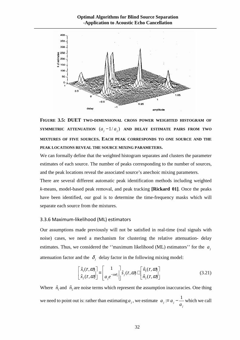
32


FIGURE 3.5: DUET TWO-DIMENSIONAL CROSS POWER WEIGHTED HISTOGRAM OF

SYMMETRIC ATTENUATION ( 1/ )j ja a− AND DELAY ESTIMATE PAIRS FROM TWO

MIXTURES OF FIVE SOURCES. EACH PEAK CORRESPONDS TO ONE SOURCE AND THE

PEAK LOCATIONS REVEAL THE SOURCE MIXING PARAMETERS .

We can formally define that the weighted histogram separates and clusters the parameter

estimates of each source. The number of peaks corresponding to the number of sources,

and the peak locations reveal the associated source’s anechoic mixing parameters.

There are several different automatic peak identification methods including weighted

k-means, model-based peak removal, and peak tracking [Rickard 01]. Once the peaks

have been identified, our goal is to determine the time-frequency masks which will

separate each source from the mixtures.

3.3.6 Maximum-likelihood (ML) estimators

Our assumptions made previously will not be satisfied in real-time (real signals with

noise) cases, we need a mechanism for clustering the relative attenuation- delay

estimates. Thus, we considered the ‘’maximum likelihood (ML) estimators’’ for the ja

attenuation factor and the jδ delay factor in the following mixing model:

1 1

2 2

1ˆ ˆ( , ) ( , )ˆ ( , )

ˆ ˆ( , ) ( , )ji j

j

x ns

x na e ωδ

τ ω τ ωτ ω

τ ω τ ω−

= +

(3.21)

Where 1n and 2n are noise terms which represent the assumption inaccuracies. One thing

we need to point out is: rather than estimatingja , we estimate 1

:j jj

a aa

= − which we call

33


the “symmetric attenuation”. That is, the attenuation is reflected symmetrically about a

centre point ( ja =0) because it has the property that the two microphone (sensor) signals

can be swapped [Makino 07b]. We can define the local symmetric attenuation estimate,

2 1

1 2

ˆ ˆ( , ) ( , )( , ) :

ˆ ˆ( , ) ( , )

x xa

x x

τ ω τ ωτ ωτ ω τ ω

= −ɶ (3.22)

It is motivated by the form of the ML estimators.

However, the difficulty with the estimators is that they require knowledge of

time-frequency supports of each source. On the other hand, the local symmetric

attenuation and delay observation estimates will cluster around the actual symmetric

attenuation and delay mixing parameters of the original sources, so we need a mechanism

for determining these clusters.

The estimators suggest the construction of a two-dimensional weighted histogram to

determine the clusters and the estimated mixing parameters( , )j ja δ . Thus, the mixing

parameters can be extracted by locating the peaks in the histogram. In this review, we

won’t go over much mathematics involved in the mixing model, but well explained the

basic DUET BSS algorithm theory

3.3.7 Summary of DUET Algorithm

1) Construct time-frequency representations 1( , )x τ ω and 2ˆ ( , )x τ ω from anechoic

matrix 1( )x t and 2( )x t .

2) Calculate the mixing

parameters 2 1 2

1 2 1

ˆ ˆ ˆ( , ) ( , ) ( , )1( ( , ), ( , )) ,

ˆ ˆ ˆ( , ) ( , ) ( , )

x x xa

x x x

τ ω τ ω τ ωτ ω δ τ ωτ ω τ ω ω τ ω

−= − ∠

ɶɶ .

3) Construct a 2D smoothed weighted histogram for all weights associated with

time-frequency plant.

4) Locate peaks and find peak centres which determine the mixing parameter estimates

5) Construct time-frequency binary masks for each peak centre ( , )j ja δɶɶ via indicator

functions ( , )jM τ ω for each source and separate the sources by partitioning.

6) Apply each mask to the appropriately alighted mixtures.

7) Convert each estimated source time-frequency representation back into the time

domain.

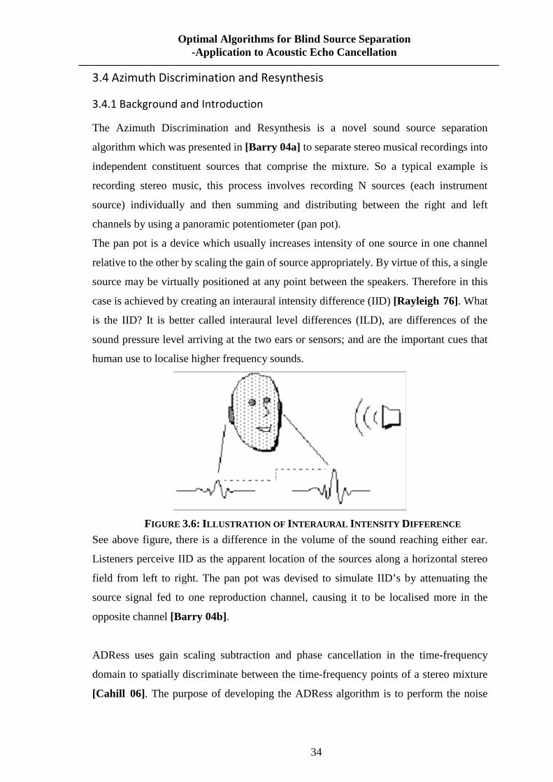
34


3.4 Azimuth Discrimination and Resynthesis

3.4.1 Background and Introduction

The Azimuth Discrimination and Resynthesis is a novel sound source separation

algorithm which was presented in [Barry 04a] to separate stereo musical recordings into

independent constituent sources that comprise the mixture. So a typical example is

recording stereo music, this process involves recording N sources (each instrument

source) individually and then summing and distributing between the right and left

channels by using a panoramic potentiometer (pan pot).

The pan pot is a device which usually increases intensity of one source in one channel

relative to the other by scaling the gain of source appropriately. By virtue of this, a single

source may be virtually positioned at any point between the speakers. Therefore in this

case is achieved by creating an interaural intensity difference (IID) [Rayleigh 76]. What

is the IID? It is better called interaural level differences (ILD), are differences of the

sound pressure level arriving at the two ears or sensors; and are the important cues that

human use to localise higher frequency sounds.

FIGURE 3.6: ILLUSTRATION OF INTERAURAL INTENSITY DIFFERENCE See above figure, there is a difference in the volume of the sound reaching either ear.

Listeners perceive IID as the apparent location of the sources along a horizontal stereo

field from left to right. The pan pot was devised to simulate IID’s by attenuating the

source signal fed to one reproduction channel, causing it to be localised more in the

opposite channel [Barry 04b] .

ADRess uses gain scaling subtraction and phase cancellation in the time-frequency

domain to spatially discriminate between the time-frequency points of a stereo mixture

[Cahill 06]. The purpose of developing the ADRess algorithm is to perform the noise

35


reduction in mobile or other communication applications. Like other sound source

separation algorithms, it has a mathematics model. So we will discuss more detailed in

ADRess methodology based on its discrete time mixing model in the next chapter.

3.4.2 ADRess Methodology

ADRess can be described as the mixing model for a channel audio and the following

discrete time mixing model defined as:

1

0

( ) ( ), 1,..., 1j

i ii

l n pl s n for n N−

== = −∑ (3.23)

1

0

( ) ( ), 1,..., 1j

i ii

r n prs n for n N−

== = −∑ (3.24)

Where ( )l n and ( )r n are the left and right mixed stereo signals, ipl and ipr are the

panning coefficients for the thi independent source ( )is n (note: these two coefficients

defined the amount we want to scale the volume (or pan) of the source in the left and right

channels),j is the number of sources and N is the length of the mixtures in the audio

samples.

In fact, we can look at these signals in the frequency domain by performing a short-time

Fourier transform (STFT) on one sample frame of the time signal. It means the algorithm

takes these two signals as its initial input data and then divides them into short

overlapping frames. These frames are transformed into the frequency domain using the

Fourier Transform [Cahill 06] using the following equations:

1

0

( , ) ( ) ( )j nNN

fn

l w n l n eω

τ ω τ−−

=

= −∑ (3.25)

1

0

( , ) ( ) ( )j nNN

fn

r w n r n eω

τ ω τ−−

=

= −∑ (3.26)

where 2 fω π= is sample rate, N is the frequency sampling factor and2 / Nπ is the

frequency sampling interval. w is usually a Hamming window and τ is the frame

number.

From the equation (3.23) and (3.24), the ratio of the left and right panning coefficients

pl andpr of the thi source can be expressed as:

( ) /i ig i pl pr= (3.27)

Similarly,

36


( ).l ipl g i pr= (3.28)

Where ( )g i is also called the intensity ratio. Adjust the intensity ratio to control the

volume (or pan) between the right and left channel. Equation 3.28 implies we can scale

the right channel to the same volume as the left channel for a given source( )is n . In fact, if

we can expect to subtract the two audio channels after performing the scaling, then the

source ( )is n can be cancelled out. (i.e. ( ). 0l g i r− = ) Similarly as scaling the left

channel which when subtracted from the right channel ( i.e. ( ). 0r g i l− = ) will be

cancelled out as well. The question is how to define the gain scales factor when the

panning coefficients are unknown as is the case of a stereo recording. The gain scale

factors are defined as follows:

( ) .(1/ )g i i β= (3.29)

for all i and for 0 i β≤ ≤ where i and β are integer values.

From equations (3.25) (3.26)fl and fr are short time frequency domain representations of

the left and right channel respectively and these equations also indicate to create a

frequency-azimuth plane for the left and right channel individually. In equation (3.29) the

azimuth resolution β refers to how many equally spaced gain scaling values of g we

will use to construct the frequency azimuth plane. Thus, right and left channel

azimuth-frequency planes are created according to the following equation:

( , , ) ( , ) ( ). ( , )f fAzl i r g i lτ ω τ ω τ ω= − (3.30)

( , , ) ( , ) ( ). ( , )f fAzr i l g i rτ ω τ ω τ ω= − (3.31)

for the integer values of i such that 0 i β≤ ≤ . Depending on the choice of β , the

algorithm can create different resolution azimuth planes. Also large value of β will

achieve more accurate azimuth discrimination but will increase the Fourier

computational load because the frequency –azimuth plane will be an N β× array for

each channel. In equation (3.30) (3.31), combining Azl and Azrcreates the azimuth

frequency plane of the mixture, here the “azimuth” we mentioned is purely a function of

the intensity ration, created by the pan pot.

37


FIGURE 3.7: FREQUENCY-AZIMUTH PLANE . PHASE CANCELLATION HAS OCCURRED

WHERE THE NULLS APPEAR AS SHOWN . It can be seen that the arrows point out the cancellation points along the azimuth axis. For

each frequency, there exist peaks (see figure 3.7) of varying magnitude resulting from the

phase cancellations or the gain scale subtraction process. These peaks converge to a

minimum value or even null (see figure 3.8), which corresponds to the location of that

frequency within the azimuth plane. In the ADRess algorithm, for the purpose of

resynthesis and so we need to invert these nulls, since the amount of energy lost through

cancellation is proportional to the actual energy contributed by the source [Coyle 07].

FIGURE 3.8: BY INVERTING THE NULLS OF THE FREQUENCY AZIMUTH COMPOSITION

THE FREQUENCY COMPOSITION OF EACH SCORE CAN BE CLEARLY SEEN

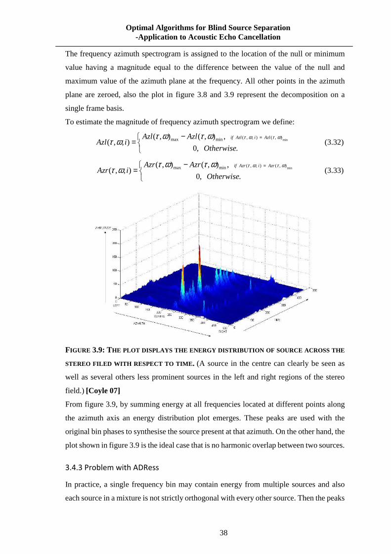
38


The frequency azimuth spectrogram is assigned to the location of the null or minimum

value having a magnitude equal to the difference between the value of the null and

maximum value of the azimuth plane at the frequency. All other points in the azimuth

plane are zeroed, also the plot in figure 3.8 and 3.9 represent the decomposition on a

single frame basis.

To estimate the magnitude of frequency azimuth spectrogram we define:

min ( , , ) ( , )max min( , ) ( , ) ,

( , , )0, .

if Azl i AzlAzl AzlAzl i

Otherwise

τ ω τ ωτ ω τ ωτ ω

=−=

(3.32)

min ( , , ) ( , )max min( , ) ( , ) ,

( , , )0, .

if Azr i AzrAzr AzrAzr i

Otherwise

τ ω τ ωτ ω τ ωτ ω

=−=

(3.33)

FIGURE 3.9: THE PLOT DISPLAYS THE ENERGY DISTRIBUTION OF SOURCE ACROSS THE

STEREO FILED WITH RESPECT TO TIME . (A source in the centre can clearly be seen as

well as several others less prominent sources in the left and right regions of the stereo

field.) [Coyle 07]

From figure 3.9, by summing energy at all frequencies located at different points along

the azimuth axis an energy distribution plot emerges. These peaks are used with the

original bin phases to synthesise the source present at that azimuth. On the other hand, the

plot shown in figure 3.9 is the ideal case that is no harmonic overlap between two sources.

3.4.3 Problem with ADRess

In practice, a single frequency bin may contain energy from multiple sources and also

each source in a mixture is not strictly orthogonal with every other source. Then the peaks

39


of these frequencies drift away from a source position and lead to locate at an erroneous

azimuth where there may or may not be a source. In other words: there are two or more

sources contributing to one frequency bin of the STFT and this results in sources not

grouping perfectly on the azimuth planes. This is called “azimuth-smearing

phenomenon” which results in frequencies being excluded from the resynthesis of the

target source. Therefore, an “azimuth subspace width” H is defined, such that1 H β≤ ≤ .

This permits including peaks that have drifted away from the target azimuth in the

resynthesis of the source. Two types of “azimuth subspace width”H are:

• A wide azimuth subspace will result in worse rejection of nearby sources.

• A narrow azimuth subspace will lead to poor resynthesis and missing harmonics

(peak).

Meanwhile, an extra term the “discrimination index”d is also introduced at this point,

where 0 d β≤ ≤ . This index, d , along with the azimuth subspace width, H , will define

what portion of the frequency-azimuth plane is extracted for resynthesis.

3.4.4 Resynthesis

Collectively d and H will define what portion of the azimuth frequency plane will be

used for resynthesis. In practice, we set the azimuth subspace to span [Barry 04b] [Barry

04c] from ( / 2)d H− to ( / 2)d H+ . The peaks for resynthesis are extracted using,

/2

/2

( , ) ( , , )i d H

i d H

Y Az iτ ω τ ω= +

= −

= ∑ (3.34)

Where Az is the combinedAzl Azr− inverse azimuth frequency plane and Y is the output

time frequency points. The resultant Y must be left and right channel, each channel

containing only the bin magnitudes pertaining to a particular azimuth subspace as defined

by d and H. The bin phases from the original FFT are used to resynthesis the extracted

source. Thus, the magnitude and phase component of each bin are combined and

converted from polar to complex form. The azimuth subspace is then resynthesisd using

the Inverse Short Time Fourier Transform (ISTFT), see equation 3.35.

1

1( ) ( , )

j nNN

k

X n Y eω

τ ωτ

+

=

= ∑ (3.35)

WhereX is the output signal rendition. The resynthesisd time frames are then recombined

using a simple overlap and add scheme [Barry 04c].

40


In practice, the resynthesis is not perfect due to the fact of the power spectrum for each

frame and source is an estimate. The windowing function (hamming window) is not

preserved and therefore the frames at the output do not overlap perfectly. At the frame

boundaries, there may be some distortion. Ideally, we need smoother frame transitions, so

it can be resolved by multiplying the output frame by a suitable windowing function

[Barry 04c]. In another words, by controlling the parameter d and H be set subjectively

until the required separation is achieved.

3.5 Conclusions

ICA is a very general-purpose statistical technique that is used to find underlying factors

by analyzing a set of observed random data. These observed random data are linearly

transformed into components that are maximally independent of each other. ICA was

originally developed to deal with sound source separation for audio processing, but now

has been widely used in many different areas such as biomedical signal processing, image

processing, telecommunications, and econometrics. In addition, ICA can be estimated as

a latent variable model. There are two approaches that can be used to estimate ICA:

optimization of the maximum of non-gaussianity can be used for the estimation of the

ICA model; alternatively, maximum likelihood estimation or minimization of mutual

information can also be used to estimate ICA.

PCA is a widely used statistical technique in many applications. It can be used to perform

data compression while it can also be used to analyse data sets. However, PCA is not

commonly associated with sound source separation. The fact that all the eigenvectors are

orthogonal makes this technique useless for most mixtures, except artificial constructions

where the columns of the mixing matrix are orthogonal. Even though this method is of

little use for the separation of audio signals, this discussion gives a geometrical

interpretation of the separation problem that can be useful in the following discussion of

other techniques.

DUET is another technique which can be used for sound source separation. Theoretically

it can separate any number of sources using just two mixed records if the sources are

W-Disjoint orthogonal with each other. This technique is based on the fact that all

frequencies coming from one source should have the same attenuation and time delay

41


relative to the microphones. DUET is well suited to human speech separation; however,

due to its assumption that all sources are W-Disjoint orthogonal with each other, its

performance of musical signal separation is not as good as human speech separation.

Nevertheless, using DUET to separate anechoically mixed and stereophonic music

streams is an interesting research topic.

The ADRess algorithm is a new technique that can perform sound source separation by

using the idea that sources occupy unique azimuth positions in the frequency-azimuth

plane. This algorithm breaks down the sound mixture into frequency-azimuth subspaces,

these subspaces can then be resynthesised according to different sources, resulting in

source separation. In addition, the ADRess algorithm is able to separate multiple sources

from only two mixtures. This feature makes it capable of enhancing sound quality in

many areas. One of the possible applications is that by adding a second microphone in the

mobile phone, the algorithm can perform noise reduction and sound quality enhancement

in the mobile communication.

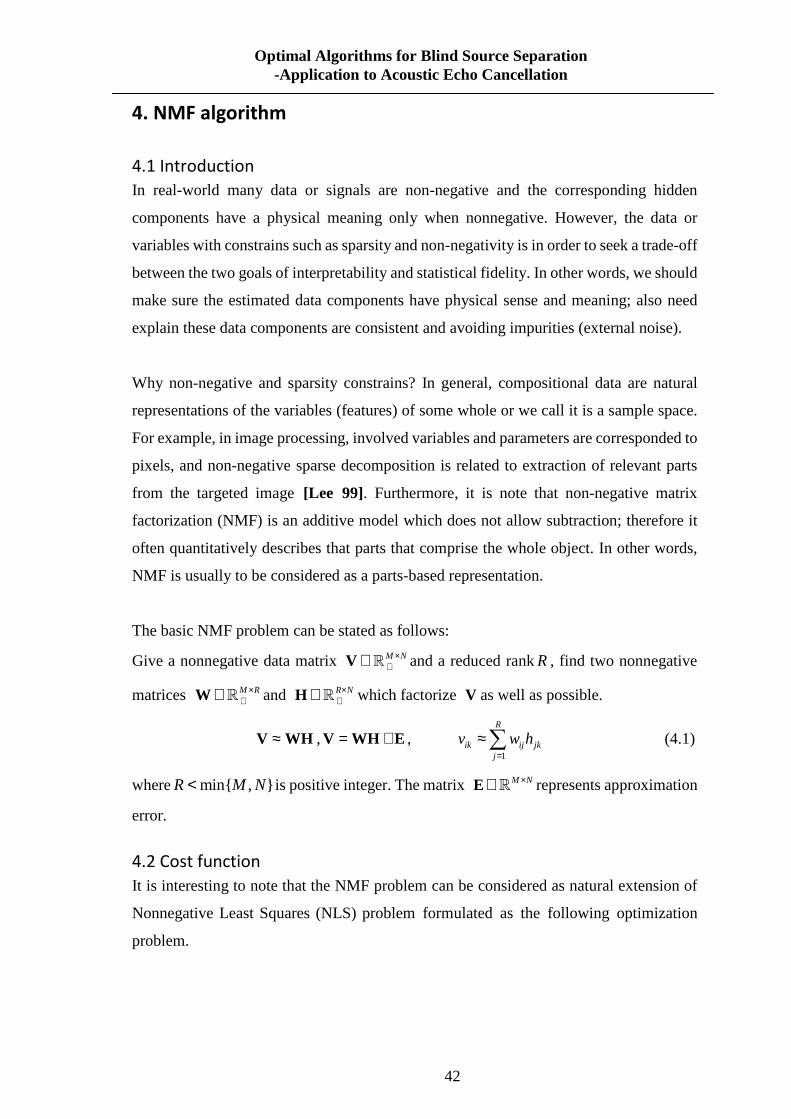
42


4. NMF algorithm

4.1 Introduction

In real-world many data or signals are non-negative and the corresponding hidden

components have a physical meaning only when nonnegative. However, the data or

variables with constrains such as sparsity and non-negativity is in order to seek a trade-off

between the two goals of interpretability and statistical fidelity. In other words, we should

make sure the estimated data components have physical sense and meaning; also need

explain these data components are consistent and avoiding impurities (external noise).

Why non-negative and sparsity constrains? In general, compositional data are natural

representations of the variables (features) of some whole or we call it is a sample space.

For example, in image processing, involved variables and parameters are corresponded to

pixels, and non-negative sparse decomposition is related to extraction of relevant parts

from the targeted image [Lee 99]. Furthermore, it is note that non-negative matrix

factorization (NMF) is an additive model which does not allow subtraction; therefore it

often quantitatively describes that parts that comprise the whole object. In other words,

NMF is usually to be considered as a parts-based representation.

The basic NMF problem can be stated as follows:

Give a nonnegative data matrix M N×+∈V ℝ and a reduced rankR, find two nonnegative

matrices M R×+∈W ℝ and R N×

+∈H ℝ which factorize V as well as possible.

≈V WH , = +V WH E , 1

R

ik ij jkj

v w h=

≈∑ (4.1)

where min{ , }R M N< is positive integer. The matrix M N×∈E ℝ represents approximation

error.

4.2 Cost function

It is interesting to note that the NMF problem can be considered as natural extension of

Nonnegative Least Squares (NLS) problem formulated as the following optimization

problem.

43


In the NMF algorithm, Lee and Seung [Lee 99] suggested an approach similar to that

used in Expectation- Maximization algorithms to iteratively update the factorization

based on a given objective function. Two conventional NMF algorithms were introduced

by them, each seeking to minimize a different object function or distance measure with a

particular iterative update strategy chosen for its implementation ease and each

optimizing its own measure of reconstruction quality: first measure is the Euclidean

distance,

21

( , , )2EDD = −V W H V WH (4.2)

In computing an NMF using the Euclidean Distance Algorithm, we wish find factors,

W andH , that minimize the objective function. In order to balance algorithm complexity

and convergence speed and we use the following multiplicative update rules:

[ ]

[ ]

Tij

ij ij Tij

w w←VH

WHH,

[ ]

[ ]

Tjk

ij ij Tjk

h h←W V

W WH (4.3)

Where [ ] ij⋅ indicates that the noted divisions and multiplications are computed

element-by element.

The second objective function commonly used in practical measure is the divergence; we

called a generalized version of the Kullback-Leibler divergence, (also called the

I-divergence) [Sajda 03]

( || , ) log [ ]

[ ]ik

KL ik ik ikik ik

vD v v

= − +

∑V W H WH

WH (4.4)

The above objective functionKLD is not a distance measure due to it is not symmetric in

V and approximation .WH In this case, KLD reduces to the Kullback-Leibler

information measure used in statistics that quantifies in bits how close a probability

distributionV is to a model distributionWH , zero if the distributions match exactly and

can potentially equal infinity. In addition, this object function is related to likelihood of

generating the columns inV from the basisW and coefficientsH . Same again, in order to

balance complexity and convergence speed, the following update rules are commonly

used:

1

1

( / [ ] )N

ik ik jkkij ij N

jkk

v hw w

h=

=

← ∑∑

WH, 1

1

( / [ ] )M

ij ik ikijk jk M

iji

w vh h

w=

=

← ∑∑

WH (4.5)

44


where the subscripts again indicate element by element division or multiplications.

Currently most existing approaches minimize only one kind of cost function by

alternately switching between sets of parameters. In this thesis we use a more general

approach (algorithm) in which instead of one cost function we use called multi-layer

NMF using alternating minimization of two cost functions; one of them is minimized

with respect toW and the other one with respect toH . The following pseudo code

represents most NMF algorithm to AEC application discussed in next two chapters.

Algorithm 4.1: Multi-layer NMF two cost function m inimization

Input: M N×+∈V ℝ ; input matrix data. R: rank of factorization

Output: M R×+∈W ℝ and R N×

+∈H ℝ ; the given cost functions are minimized.

1 Begin

2 H = V , W = I

3 for l = 1 to L do

4 Initialize randomly ( )lW and ( )lH

5 repeat

6 ( ){ }( )

( ) 1 ( ) ( )0arg min

ll l lD

≥=

WW H W H� for fixed ( )lH

7 ( ){ }( )

( ) 2 ( ) ( )0arg min

ll l lD

≥=

HH H W H� for fixed ( )lW

8 until a convergence condition is met

9 ( )l=H H

10 ( )l←W WW

11 end

12 End

Table 4.1: Multi-layer NMF using alternating minimi zation of two cost function

Here is the MATLAB function to perform basic NMF algorithm which is mainly used

in the rest of the thesis:

function [H,W] = NMF(spec,R,num_iter);

45


V = abs(spec(:,1:513))'; index = size(V); % must be nonnegative M = index(1,1); N = index(1,2); W = rand(M,R); % random initialization H = rand(R,N); num_iter = 100; % can be adjusted for i = 1:1:num_iter W = W.*((V./(W*H+1e-9))*H')./(ones(M,N)*H'); H = H.*(W'*(V./(W*H+1e-9)))./(W'*ones(M,N)); end

Table 4.2: Standard NMF Algrithm in MATLAB Form

4.3 Initialization of NMF

The motivation behind NMF is that besides the dimensionality reduction sought in

many image or signal processing applications. As defined, the NMF problem is a more

general instance of the case where the two nonnegative matrices whose product exactly

equals the original matrix. In common sense, there is no guarantee that an exact

nonnegative factorization exists for arbitrary R which is rank of approximation. It is

known, however, that if 0≥V , then the nonnegative rank and

nonnegativeW andH having that number as rank so thatV = WH holds exactly

[Gregory 83]. Furthermore, NMF is a part of nonconvex optimization problem with

inequality constraints and iterative methods become necessary for its solution

[Bertsekas 99][Salakhutdinov 03]. However, the current NMF algorithms typically

converge comparative slowly and then at local minima. Most algorithms for NMF are

iterative and required initial values ofW and H , and many authors prescribe

initializing W andH with random non-negative numbers. A suitable chosen initialization,

can lead to faster convergence, and since the solution of most NMF algorithm problems

is not unique, different initializations can lead to different solutions.

4.3.1 Optimization problem

The solution and convergence provided by the NMF algorithm usually highly depend

on initial conditions, typically starting guess values, especially in a multivariate context.

Therefore, it is important to have efficient and consistent ways for initialization

matricesW andH . Due to the iterative nature of NMF algorithms, most of them in the

46


literature use random nonnegative initialization for ( W ,H ). Iterates converge to a local

minimum and poor initializations also often result in slow convergence, and in certain

instances may lead even to an incorrect or irrelevant solution which we aim to. The

problem of selecting an appropriate starting point or starting initialization matrices

becomes even more complicated for large-scale NMF problems [Dhillon 01] and when

certain structures or constraints are imposed on the factorized matrices involved. In the

real time case, initialization in NMF plays a key role since the objective function to be

minimized may have local minima, and the intrinsic alternating minimization in NMF is

nonconvex, even though the objective function is strictly convex with respect to one set

of variables. The issues of initialization in NMF have been widely discussed in the

literature [Baeza 92] [Carmona 06] [Ruspini 69].

4.3.2 Basic initialization for NMF algorithm

As a rule of thumb, we can obtain a robust initialization using the following three steps

which the main idea is to find better initial estimates with the multi-start initialization

algorithm:

• First, we can generate S (number of restarts) by a search method to initial

matricesW andH . This could be based on random starts or the output from a

simple conventional NMF algorithm. The parameter S depends on the number of

required iterations. We typically set S between 15 and 20.

• Run a specific NMF algorithm for each set of initial matrices and with a fixed

but small number of iterations (15-20). As a result, the NMF algorithm provides

S initial estimates of the matrices( )sW and ( )sH .

• Select the estimates (“candidates”), we denoted that min( )sW and min( )sH

correspond to the lowest value of the cost function (the best likelihood) among

the R trials as initial values for the final factorization.

The following pseudo code represents above steps:

Algorithm 4.2: Multi-start initialization

47


Input: M N×+∈V ℝ : input matrix data,

R: rank of factorization, S: number of restarts,

Kinit, Kfin: number of alternating steps for initialization and completion

Output: M R×+∈W ℝ and R N×

+∈H ℝ ; the given cost functions are minimized.

1 Begin

2 parfor s = 1 to S do % process in parallel mode

3 Initialize randomly (0)W or (0)H

4 { } ( )( ) ( ) ( ) ( ), nmf_algorithm , , ,s s s sinitK←W H V W H

5 ( )( ) ( )s ssd D= V W H�

6 endfor

7 min 1arg min s S ss d≤ ≤=

8 { } ( )min min( ) ( ), nmf_algorithm , , ,s sfinK←W H V W H

9 End

Table 4.3: Multi-start initialization to initial NM F alogorithm

Thus, the multi-start initialization selects the initial estimates forW andH which give

the steepest decrease in the assumed objective (cost) function ( )D V WH� via

alternating steps.

4.3.3 Termination condition

In many practical situations, the iterations usually continue until some combinations of

termination conditions or stopping criteria are satisfied. There are several possible

stopping criteria for the iteration algorithm used in NMF:

• The cost function achieves a zero-value or a value just below a given thresholdε ,

also during the NMF divergence updating, the stopping criterion can be adjusted,

for example: Frobenius norm of cost function,

( ) 2( ) ( ) ( )ˆ ˆk k kF

FD ε= − ≤V V V V� , ( ) ( ) ( )ˆ k k k=V W H (4.6)

V is estimated value.

• There is little or no improvement between successive iterations in the

minimization of a cost function, for example: Frobenius norm of the estimated

matrices,

48


( ) 2( 1) ( 1) ( ) ( ) ( 1)ˆ ˆ ˆ ˆk k k k kF

FD ε+ + += − ≤V V V V� (4.7)

or Ratio of the distance

( ) ( 1)

( )

k kF F

kF

D D

Dε

−−≤ (4.8)

• There is little or no change in the updates for factor matricesW andH .

• The number of iterations achieves or exceeds a predefined maximum number of

iterations and the maximum number of iterations also can be adjusted.

4.4 Convolutive NMF

The Convolutive NMF (CNMF) is a natural extension and generalization of the

standard NMF. The standard NMF represents regularly repeating patterns which span

multiple columns of theV matrix using a number of different bases to describe the entire

sequence. CNMF uses a single basis function that spans the pattern length. This kind of

situation can be very frequently found when analysing audio signals. In the Convolutive

NMF, we process a set of nonnegative matrices or patterns which are horizontally

shifted (or time delayed) versions of the primary matrix W [Zass 05]. In the simplest

form the CNMF can be defined as (see Figure: 4.1)

FIGURE 4.1: ILLUSTRATION OF CONVOLUTION NMF

49


In the previous section, we saw the NMF uses a matrix product ≈V WH to reconstruct

the estimated data matrixV , in the convolutive Non-Negative Matrix Factorization they

extend this expression to:

1

0

T t

tt

− →

=≈ ⋅ +∑V W H E (4.9)

where M N×+∈V ℝ is a given input data matrix to be decomposed, M R

t×

+∈W ℝ is a set of

unknown nonnegative matrices,0

R N→

×+= ∈H H ℝ is the matrix representing coding

information of the source (such as position of activation and it’s amplitude). Heret→H is a

t column shifted version ofH . In other words, t→H denotes the t positions (columns)

shifting operator to the right, with the columns shifted in from outside the matrix set to

zero. This shift (sample-delay) is performed by a basic operator denoted as( )i→

i .

( )i←

i performs the reverse. The matrix M N×∈E ℝ represents approximation error.

The i th column of tW describes the spectrum of the i object t time steps after the object

has begun.

Equation 4.12 is a summation of convolution operations between corresponding elements

from a set of two-dimensional basesW and a set of weightsH .

The set of i th columns of ( )tW defines a two-dimensional structure. This matrix will be

shifted and scaled by convolution across the axis of t with the i th row ofH . The resulting

reconstruction will be a summation of all the basis convolution results for each of the R

bases.

The estimation of the appropriate set of matrices( )tW and H to approximate V is based

on the framework of NMF that Lee and Seung used in [Lee 99]. In accordance to the

NMF cost function, they defined the Convolutive NMF cost function as:

ˆ|| | ||ˆ FD In

= • − +

VV V V

V (4.10)

Where V is the approximation of V defined as:

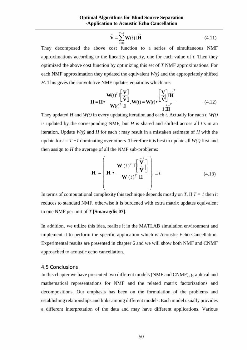
50


1

0

ˆ ( )T t

t

t− →

== ⋅∑V W H (4.11)

They decomposed the above cost function to a series of simultaneous NMF

approximations according to the linearity property, one for each value of t. Then they

optimized the above cost function by optimizing this set of T NMF approximations. For

each NMF approximation they updated the equivalent W(t) and the appropriately shifted

H. This gives the convolutive NMF updates equations which are:

( )

ˆ ˆ, ( ) ( )

( ) 11

TtT

TT t

tt t

t

→

→

⋅ ⋅ = • = •⋅ ⋅

V VW H

V VH H W WW

H (4.12)

They updated H and W(t) in every updating iteration and each t. Actually for each t, W(t)

is updated by the corresponding NMF, but H is shared and shifted across all t’s in an

iteration. Update W(t) and H for each t may result in a mistaken estimate of H with the

update for t = T −1 dominating over others. Therefore it is best to update all W(t) first and

then assign to H the average of all the NMF sub-problems:

( )ˆ

,( ) 1

t

T

T

tt

t

← ⋅ = • ∀ ⋅

VW

VH HW

(4.13)

In terms of computational complexity this technique depends mostly on T. If T = 1 then it

reduces to standard NMF, otherwise it is burdened with extra matrix updates equivalent

to one NMF per unit of T [Smaragdis 07].

In addition, we utilize this idea, realize it in the MATLAB simulation environment and

implement it to perform the specific application which is Acoustic Echo Cancellation.

Experimental results are presented in chapter 6 and we will show both NMF and CNMF

approached to acoustic echo cancellation.

4.5 Conclusions

In this chapter we have presented two different models (NMF and CNMF), graphical and

mathematical representations for NMF and the related matrix factorizations and

decompositions. Our emphasis has been on the formulation of the problems and

establishing relationships and links among different models. Each model usually provides

a different interpretation of the data and may have different applications. Various

51


equivalent representations have been presented which will serve as a basis for the

development of learning algorithms in next two chapters.

52


5. Acoustic echo cancellation MATLAB experiment

This chapter is organized as follows: in section 5.1 we present a detailed description of

numerical aspects of the Least Mean Square (LMS) algorithm. The second section is

focused on the different versions of the LMS algorithm simulation in MATLAB and an

experiment result will be presented. In section 6.3, we use two set of NMF experiments

(standard NMF and convolution NMF) to perform AEC. The convolution NMF

experiment is based on the process of using standard NMF. The purpose of these

experiments is finding a better solution for AEC and comparing the results with LMS

counterparts.

5.1 Least Mean Square Solution for Acoustic Echo Cancellation

5.1.1 Steepest Decent Algorithm

The Steepest Decent algorithm is a method of gradient decent minimization or an

“adaptive” approach. We can find a single global minimum corresponding to the

optimum weights based on the quadratic cost function.

Formally the gradient is defined as:

J

J∂= ∇ =∂wgw

(5.1)

Sinceg is the direction of steepest ascent−g gives us the direction of steepest descent.

The iterative procedure of the steepest or gradient descent method as follows:

Start with an arbitrary initial weights vectors , 0k k =w

Calculate the gradient 2[ ]k kk

J∂= = −∂

g Rw pw

Update the weights vector in the direction of steepest descent using the rule:

1k k kµ+ = −w w g (5.2)

Whereµ is a positive constant known as the step size or learning rate.

Set 1k k= + and repeat until the algorithm converges.

53


5.1.2 LMS Derivation

It is simple to derive the Least-Mean-Square based on the steepest decent algorithm. We

have Mean Square Error (MSE) cost function 2( ) [ ] 2 T TkJ E d= − +w w p w Rw ,

both kd and kx are jointly wide-sense stationary. Also we have the Wiener Solution (Eq.

5.3) * 1−=w R p .

Therefore, a steepest-decent-based algorithm can be used to search the Wiener solution as

follows:

1

[ 2 2 ]

2 [ ]

2

kk k

k k k k

Tk k k k k k

k k k

d

e

µµ

µµ

+ = −= − − +

= + −= +

ww w g

w p R w

w x x x w

w x

(5.3)

This is the Least-mean-square algorithm that was proposed by Bernard Widrow in the late

1960s [Widrow 60].

5.1.3 Gradient behaviour

The ideal search direction is on the MSE surface for the optimum coefficient vector

solution (Eq. 5.8). In the LMS algorithm, instantaneous estimates ofR andp are used to

determine the search direction:

2[ ]k Tk k k k kd= −wg x x w x (5.4)

In general, the LMS gradient direction has the tendency to approach the ideal gradient

direction since for a fixed coefficient vector (filter weight factor)w and its convergence

behaviour is different from the steepest-decent algorithm counterpart. Hence,

{ }ˆ( ) 2 [ ] [ ]

k Tk k k kE E E d= −

=w

w

g x x w x

g (5.5)

Under an ergodic condition, the average direction tends to wg with a fixedw vector when

calculated for a large number of inputs and reference signals.

5.1.4 Condition for the LMS convergence

Determine the range of convergence factorµ of the LMS algorithm. Firstly, we should

know the error in the filter coefficients as related to the ideal coefficient vector*w , then

gives:

*k k∆ = −w w w . (5.6)

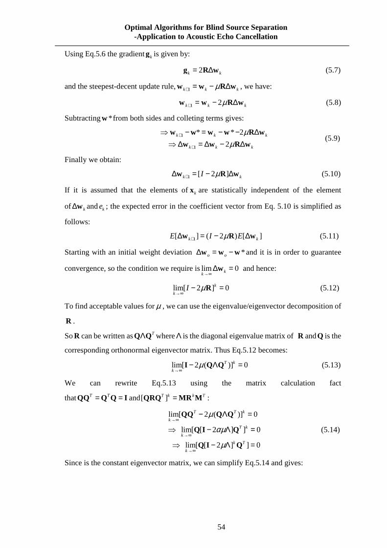
54


Using Eq.5.6 the gradientkg is given by:

2k k= ∆g R w (5.7)

and the steepest-decent update rule,1k k kµ+ = − ∆w w R w , we have:

1 2k k kµ+ = − ∆w w R w (5.8)

Subtracting *w from both sides and colleting terms gives:

1

1

* * 2

2k k k

k k k

µµ

+

+

⇒ − = − − ∆⇒ ∆ = ∆ − ∆w w w w R w

w w R w (5.9)

Finally we obtain:

1 [ 2 ]k kI µ+∆ = − ∆w R w (5.10)

If it is assumed that the elements ofkx are statistically independent of the element

of k∆w and ke ; the expected error in the coefficient vector from Eq. 5.10 is simplified as

follows:

1[ ] ( 2 ) [ ]k kE I Eµ+∆ = − ∆w R w (5.11)

Starting with an initial weight deviation *o o∆ = −w w w and it is in order to guarantee

convergence, so the condition we require islim 0kk→∞

∆ =w and hence:

lim[ 2 ] 0k

kI µ

→∞− =R (5.12)

To find acceptable values forµ , we can use the eigenvalue/eigenvector decomposition of

R .

SoR can be written as TΛQ Q whereΛ is the diagonal eigenvalue matrix of R andQ is the

corresponding orthonormal eigenvector matrix. Thus Eq.5.12 becomes:

lim[ 2 ( )] 0T k

kµ

→∞− Λ =I Q Q (5.13)

We can rewrite Eq.5.13 using the matrix calculation fact

that T T= =QQ Q Q I and[ ]T k k T=QRQ MR M :

lim[ 2 ( )] 0

lim[ [ 2 ] ] 0

lim[ [ 2 ] ] 0

T T k

k

T k

k

k T

k

µ

αµ

µ

→∞

→∞

→∞

− Λ =

⇒ − Λ =

⇒ − Λ =

QQ Q Q

Q I Q

Q I Q

(5.14)

Since is the constant eigenvector matrix, we can simplify Eq.5.14 and gives:

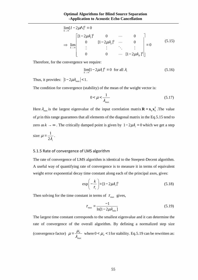
55


1

2

lim[ 2 ] 0

[1 2 ] 0 0

0 [1 2 ] 0 lim 0

0 0 [1 2 ]

k

k

k

k

k

kN

I µ

µλµλ

µλ

→∞

→∞

− Λ =

− − ⇒ =

−

⋯

⋯

⋮ ⋮ ⋱ ⋮

⋯

(5.15)

Therefore, for the convergence we require:

lim[1 2 ] 0 for all ki i

kµλ λ

→∞− = (5.16)

Thus, it provides: max1 2 1µλ− < .

The condition for convergence (stability) of the mean of the weight vector is:

max

10 µ

λ< < (5.17)

Here maxλ is the largest eigenvalue of the input correlation matrix Tk k=R x x .The value

of µ in this range guarantees that all elements of the diagonal matrix in the Eq.5.15 tend to

zero ask → ∞ . The critically damped point is given by 1 2 0iµλ− = which we get a step

size:1

2 i

µλ

= .

5.1.5 Rate of convergence of LMS algorithm

The rate of convergence of LMS algorithm is identical to the Steepest-Decent algorithm.

A useful way of quantifying rate of convergence is to measure it in terms of equivalent

weight error exponential decay time constant along each of the principal axes, gives:

exp [1 2 ]kii

k µλτ

− = −

(5.18)

Then solving for the time constant in terms of maxτ gives,

maxmin

1

ln[1 2 ]τ

µλ−=

− (5.19)

The largest time constant corresponds to the smallest eigenvalue and it can determine the

rate of convergence of the overall algorithm. By defining a normalized step size

(convergence factor) max

λµµλ

= where0 1λµ< < for stability. Eq.5.19 can be rewritten as:

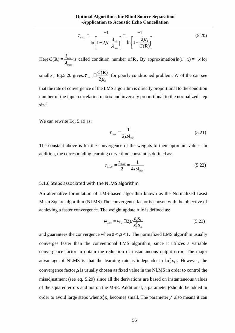
56


max

min

max

1 1

2ln 1ln 1 2

( )Cλ

λ

τµλµ

λ

− −= = −−

R

(5.20)

Here min

max

( )Cλλ

=R is called condition number ofR . By approximationln(1 )x x− = − for

smallx , Eq.5.20 gives:max

( )

2

C

λ

τµ

≅ R for poorly conditioned problem. W of the can see

that the rate of convergence of the LMS algorithm is directly proportional to the condition

number of the input correlation matrix and inversely proportional to the normalized step

size.

We can rewrite Eq. 5.19 as:

maxmin

1

2τ

µλ= (5.21)

The constant above is for the convergence of the weights to their optimum values. In

addition, the corresponding learning curve time constant is defined as:

max

min

1

2 4MSE

ττµλ

= = (5.22)

5.1.6 Steps associated with the NLMS algorithm

An alternative formulation of LMS-based algorithm known as the Normalized Least

Mean Square algorithm (NLMS).The convergence factor is chosen with the objective of

achieving a faster convergence. The weight update rule is defined as:

1 2 k kk k T

k k

eµ+ = + xw w

x x (5.23)

and guarantees the convergence when0 1µ< < . The normalized LMS algorithm usually

converges faster than the conventional LMS algorithm, since it utilizes a variable

convergence factor to obtain the reduction of instantaneous output error. The major

advantage of NLMS is that the learning rate is independent of Tk kx x . However, the

convergence factorµ is usually chosen as fixed value in the NLMS in order to control the

misadjustment (see eq. 5.29) since all the derivations are based on instantaneous values

of the squared errors and not on the MSE. Additional, a parameterγ should be added in

order to avoid large steps whenTk kx x becomes small. The parameterγ also means it can

57


overcome potential numerical instability in the update of the weights. In practise, a small

positive adaption constant ε (usually far smaller than 1) multiplies the step size to

achieve a proper compromise between the convergence rate and the misadjustment

[Haykin 02]. The updated coefficient of NLMS is given by:

1 2 k kk k T

k k

eµεγ+ = +

+x

w wx x

(5.24)

In summary, there are similar processes to the LMS algorithm as follows:

1) Initial condition: input signalx and weight vector [0, ,0]Tk =w ⋯ , 0,1,2,....k =

2) The convergence factor is0 1µ< < .

3) γ is a small constant.

Calculate the output for the current training input: Tk ky = w x

Estimate the error: k k ke d y= −

Update the weight vector: 1 2 k kk k T

k k

eµεγ+ = +

+x

w wx x

with positive constant step sizeµ .

5.1.7 Excess Mean-Square Error and Misadjustment

The LMS algorithm uses a noisy estimate of the gradient the Mean Square error (MSE).

Thus, misadjustment is defined as the ratio of the excess MSE to the minimum MSE and

is a measure the performance of the adaptive process tracks the true Wiener solution – i.e.

it is a measure of the “cost of adaptability”.

The excess in the Mean Square Error is given by:

Excess MSE = min[ ] [ ] [ ]T Tk k k kE J J E E− = ∆ ∆ = Λw w R w m m (5.25)

Since *k k∆ = −w w w and Λ is diagonal as mentioned before, this can be written as a

sum (non-matrix form):

1

2

1

[ ]N

MSE i iki

J E mλ+

==∑ (5.26)

If the LMS has converged the only variation in the weights will be due to gradient noise

causing the weights to the wander around the minimum value. Therefore,

2min[ ]ikE m Jµ≈ (5.27)

And the excess MSE formula becomes:

58


1

min min1

[ ]N

MSE ii

J J Jµ λ µ+

== =∑ tr R (5.28)

Finally, we obtain the NLMS misadjustment M ,is defined as

min

min min

[ ]Excess MSE[ ]

JM

J J

µ µ= = =tr Rtr R (5.29)

The trade-off analysis among the rate of convergence, the amount of excess mean-square

error, and the ability of the adaption to track the signal is important. Thus misadjustment

is directly proportional to step-size. We therefore have to trade rate of adaption with

accuracy as measured by misadjustment.

5.2 Using different LMS Algorithms to Perform AEC

5.2.1 Experiment principles and procedure

The experiment is about the normalized least mean square (LMS) algorithm. The

application in this experiment is echo cancellation in real-time VoIP scenario. Actually,

we recorded the speech data into MATLAB as testing data. Here we need to point out,

is that echo can’t origin from a VoIP network. But delay time due to codec and

buffering quickly makes even the slightest echo received very annoying. Echo is

generated by digital with 4 wire to analogue with 2 wire conversions either in the public

switched telephone network (PSTN). As aforementioned chapter five, there are a couple

of mechanisms to prevent echo that is ERLE (Echo Return Loss Enhance).

ERLE is often named echo canceller. ERLE is expressed in dB. The higher the value, the

better the echo canceller. Furthermore, ERLE as a function of the discrete-time index n

provides information about the convergence behaviours of the canceller. The input

signal of an echo canceller system is often a speech signal. Speech signals are

non-stationary, which makes the choice of step size rather difficult. One advantage of

the NLMS algorithm is the choice of its step size. In the previous section we have

detailed discussed LMS and NLMS in math form. In this section, we write a series

function via MATLAB simulation to perform echo cancellation. Meanwhile, we will

compare the ERLE-curves of LMS and NLMS to tell why the NLMS do work better

than the stand LMS for input speech signal with strong varying amplitude. To compare

LMS and NLMS, we also introduced another more efficient LMS algorithm named

FastLMS.

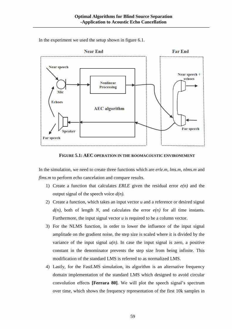
59


In the experiment we used the setup shown in figure 6.1.

FIGURE 5.1: AEC OPERATION IN THE ROOMACOUSTIC ENVIRONEMENT

In the simulation, we need to create three functions which are erle.m, lms.m, nlms.m and

flms.m to perform echo cancelation and compare results.

1) Create a function that calculates ERLE given the residual error e(n) and the

output signal of the speech voice d(n).

2) Create a function, which takes an input vector u and a reference or desired signal

d(n), both of length N, and calculates the error e(n) for all time instants.

Furthermore, the input signal vector u is required to be a column vector.

3) For the NLMS function, in order to lower the influence of the input signal

amplitude on the gradient noise, the step size is scaled where it is divided by the

variance of the input signal u(n). In case the input signal is zero, a positive

constant in the denominator prevents the step size from being infinite. This

modification of the standard LMS is referred to as normalized LMS.

4) Lastly, for the FastLMS simulation, its algorithm is an alternative frequency

domain implementation of the standard LMS which designed to avoid circular

convolution effects [Ferrara 80]. We will plot the speech signal’s spectrum

over time, which shows the frequency representation of the first 10k samples in

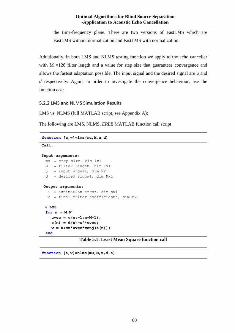
60


the time-frequency plane. There are two versions of FastLMS which are

FastLMS without normalization and FastLMS with normalization.

Additionally, in both LMS and NLMS testing function we apply to the echo canceller

with M =128 filter length and a value for step size that guarantees convergence and

allows the fastest adaptation possible. The input signal and the desired signal are u and

d respectively. Again, in order to investigate the convergence behaviour, use the

function erle.

5.2.2 LMS and NLMS Simulation Results

LMS vs. NLMS (full MATLAB script, see Appendix A): The following are LMS, NLMS, ERLE MATLAB function call script

function [e,w]=lms(mu,M,u,d)

Call: Input arguments:

mu = step size, dim 1x1 M = filter length, dim 1x1 u = input signal, dim Nx1 d = desired signal, dim Nx1 Output arguments:

e = estimation error, dim Nx1 w = final filter coefficients, dim Mx1

% LMS for n = M:N uvec = u(n:-1:n-M+1); e(n) = d(n)-w'*uvec; w = w+mu*uvec*conj(e(n)); end

Table 5.1: Least Mean Square function call

function [e,w]=nlms(mu,M,u,d,a)

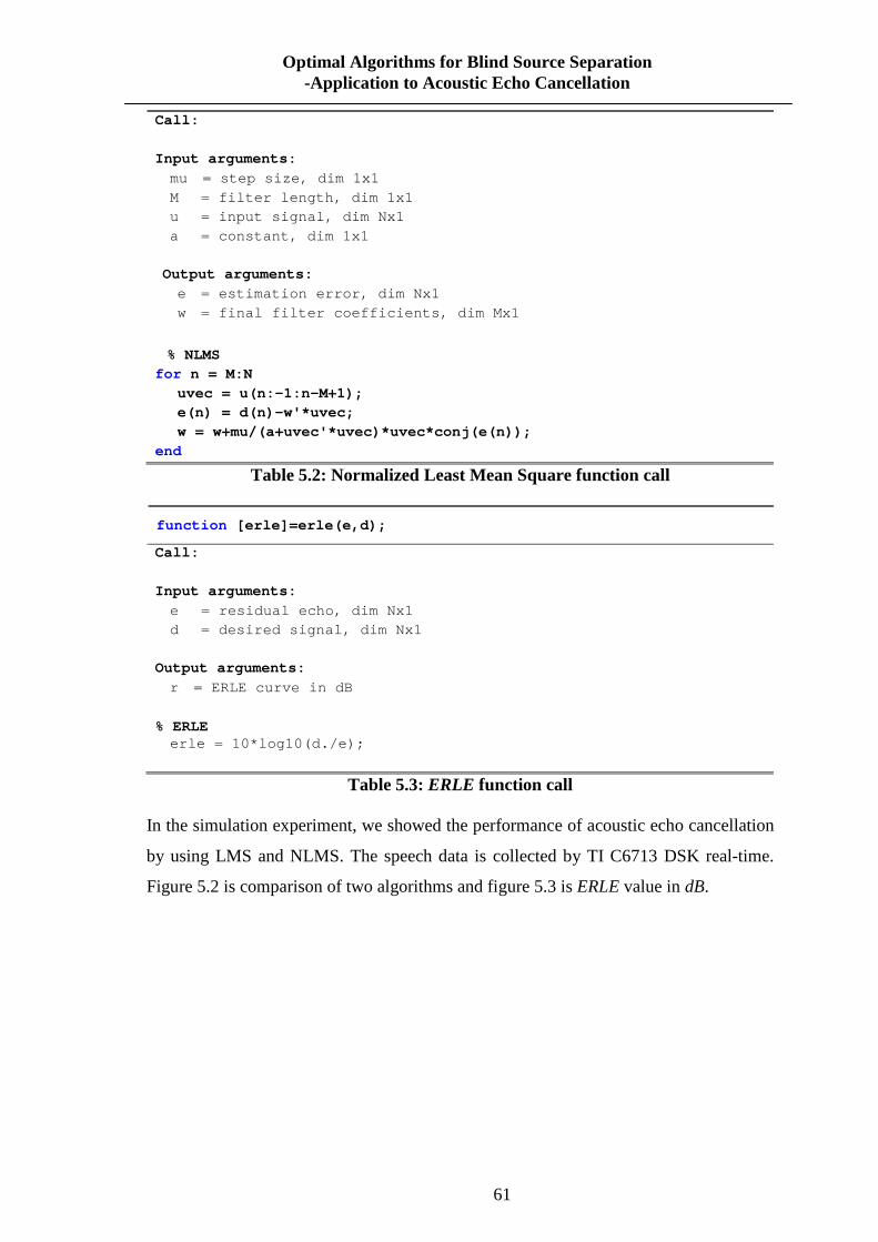
61



mu = step size, dim 1x1 M = filter length, dim 1x1 u = input signal, dim Nx1 a = constant, dim 1x1 Output arguments:


% NLMS

for n = M:N uvec = u(n:-1:n-M+1); e(n) = d(n)-w'*uvec; w = w+mu/(a+uvec'*uvec)*uvec*conj(e(n)); end

Table 5.2: Normalized Least Mean Square function call

function [erle]=erle(e,d);


e = residual echo, dim Nx1 d = desired signal, dim Nx1 Output arguments:

r = ERLE curve in dB

% ERLE erle = 10*log10(d./e);

Table 5.3: ERLE function call

In the simulation experiment, we showed the performance of acoustic echo cancellation

by using LMS and NLMS. The speech data is collected by TI C6713 DSK real-time.

Figure 5.2 is comparison of two algorithms and figure 5.3 is ERLE value in dB.

62


0 0.2 0.4 0.6 0.8 1 1.2 1.4 1.6 1.8 2

x 104

-0.06

-0.04

-0.02

0

0.02

0.04

0.06

Number of Iteration n

Am

plitu

de

Echo cancellation results

ouput d(n)

residual echo e(n) of LMS

residual echo e(n) of NLMS

FIGURE 5.2: ECHO CANCELLATION RESULTS PERFORMED BY LMS AND NLMS

Normalized LMS usually converges much more quickly and efficiently than standard

LMS at very little extra cost; NLMS is very commonly used in adaptive applications

such as AEC. Furthermore, in the LMS function algorithm step size must be

nonnegative scalar, we use max_step_size to determine a reasonable range of step size

values for the speech signals being processed, and in the NLMS function algorithm, the

step size must be a scalar between 0 and 2. Setting this step value to 1 provides the

fastest convergence.

63


0 0.2 0.4 0.6 0.8 1 1.2 1.4 1.6 1.8 2

x 104

-5

0

5

10

15

20

25

30

35

40

45


ER

LE [

dB]

ERLE Comparison

LMS

NLMS

FIGURE 5.3: ERLE VALUE COMPARISON (LMS VS. NLMS)

Iteration no. (*104) 0.1 0.4 0.6 0.8 1.2 1.4 1.6 1.8 2.0

ERLE(dB) for LMS 1.412 1.322 1.318 4.121 21.881 11.97 32.88 16.84 17.01

ERLE(dB) for NLMS 5.012 7.84 7.788 8.243 22.54 12.54 37.12 12.36 12.21

Table 5.4: ERLE value comparison (LMS vs. NLMS)

5.2.3 FastLMS and NFastLMS Simulation Results

FastLMS vs. NFastLMS (full MATLAB script, see Appendix A):

function [e,w] = fastlms(st,M,u,d,gamma,P)

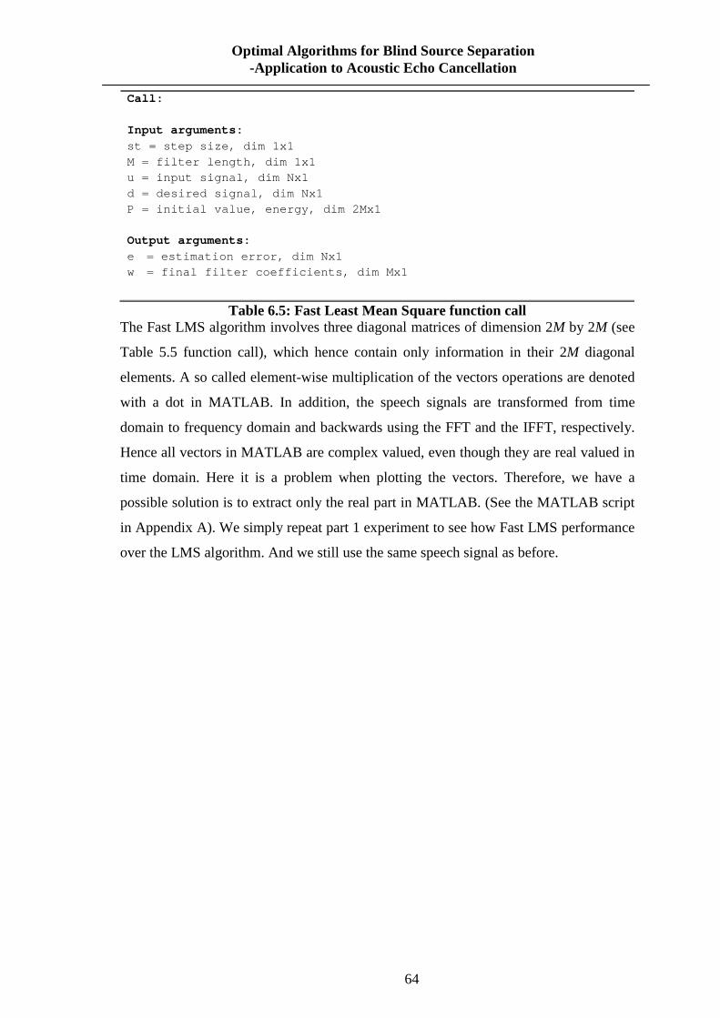
64



st = step size, dim 1x1 M = filter length, dim 1x1 u = input signal, dim Nx1 d = desired signal, dim Nx1 P = initial value, energy, dim 2Mx1 Output arguments:


Table 6.5: Fast Least Mean Square function call The Fast LMS algorithm involves three diagonal matrices of dimension 2M by 2M (see

Table 5.5 function call), which hence contain only information in their 2M diagonal

elements. A so called element-wise multiplication of the vectors operations are denoted

with a dot in MATLAB. In addition, the speech signals are transformed from time

domain to frequency domain and backwards using the FFT and the IFFT, respectively.

Hence all vectors in MATLAB are complex valued, even though they are real valued in

time domain. Here it is a problem when plotting the vectors. Therefore, we have a

possible solution is to extract only the real part in MATLAB. (See the MATLAB script

in Appendix A). We simply repeat part 1 experiment to see how Fast LMS performance

over the LMS algorithm. And we still use the same speech signal as before.

65


0 0.2 0.4 0.6 0.8 1 1.2 1.4 1.6 1.8 2

x 104

-0.06

-0.04

-0.02

0

0.02

0.04

0.06


Am

plitu

de

Echo cancellation results

output d(n)

residual echo e(n)1 of FLMS

residual echo e(n)2 of NFLMS

FIGURE 5.4: ECHO CANCELLATION RESULTS PERFORMED BY FAST LMS

0 0.2 0.4 0.6 0.8 1 1.2 1.4 1.6 1.8 2

x 104

-5

0

5

10

15

20

25

30

35

40

45


ER

LE [

dB]

ERLE

FLMS without Nor.

FLMS with Nor.

FIGURE 5.5: ERLE VALUE COMPARISON (FLMS VS. NFLMS)

66


The above figures are the investigation of ERLE for the different versions of the fast

LMS algorithm.

Iteration no. (*104) 0.4 0.6 0.8 1.2 1.4 1.6 1.8 2.0

ERLE(dB) for FLMS 0.211 0.198 2.601 4.106 2.499 8.127 3.111 4.67

ERLE(dB) for NFLMS 4.31 3.981 5.322 17.995 11.33 33.544 13.241 16.77

Table 5.6: ERLE value comparison (FLMS vs. NFLMS)

We also observe the variation of the speech signal’s spectrum over time. It can be done

using the MATLAB function spectrum, which shows the frequency representation of

the first 10k samples in the time-frequency plane. Figure 5.6 shows the spectrumgram

of residual echo using Fast LMS without normalization and figure 5.7 shows the

spectrumgram of residual echo using Fast LMS with normalization, respectively. When

we use Fast LMS with normalization and it is clear to see the overall results are better

than the performance of the counterpart without normalization

Time

Fre

quen

cy

Spectrumgram of residual echo FastLMS without Normalization.

1000 2000 3000 4000 5000 6000 7000 8000 90000

0.1

0.2

0.3

0.4

0.5

0.6

0.7

0.8

0.9

1

-120

-100

-80

-60

-40

-20

0

FIGURE 5.6: THE SPECTRUMGRAM OF RESIDUAL ECHO USING FAST LMS WITHOUT

NORMALIZATION

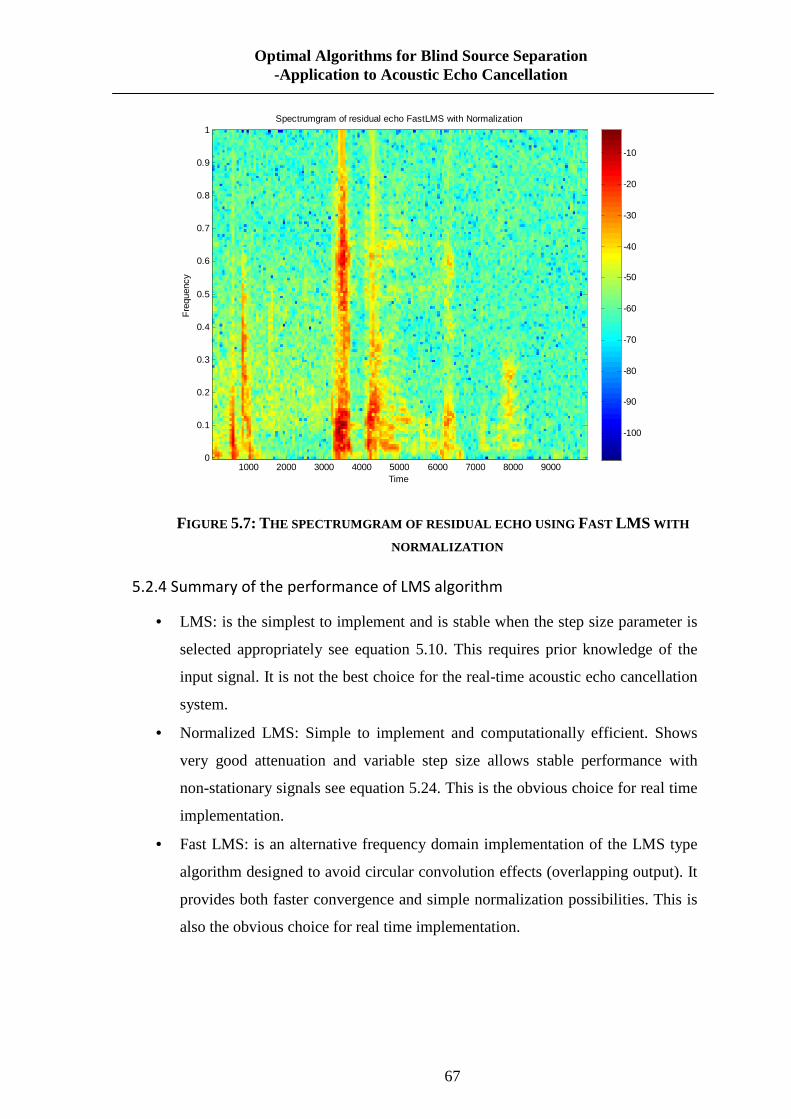
67


Time

Fre

quen

cy

Spectrumgram of residual echo FastLMS with Normalization

1000 2000 3000 4000 5000 6000 7000 8000 90000

0.1

0.2

0.3

0.4

0.5

0.6

0.7

0.8

0.9

1

-100

-90

-80

-70

-60

-50

-40

-30

-20

-10

FIGURE 5.7: THE SPECTRUMGRAM OF RESIDUAL ECHO USING FAST LMS WITH

NORMALIZATION

5.2.4 Summary of the performance of LMS algorithm

• LMS: is the simplest to implement and is stable when the step size parameter is

selected appropriately see equation 5.10. This requires prior knowledge of the

input signal. It is not the best choice for the real-time acoustic echo cancellation

system.

• Normalized LMS: Simple to implement and computationally efficient. Shows

very good attenuation and variable step size allows stable performance with

non-stationary signals see equation 5.24. This is the obvious choice for real time

implementation.

• Fast LMS: is an alternative frequency domain implementation of the LMS type

algorithm designed to avoid circular convolution effects (overlapping output). It

provides both faster convergence and simple normalization possibilities. This is

also the obvious choice for real time implementation.

68


5.3 Using NMF to Perform AEC

5.3.1 Experiment Principle and procedure

In this experiment, we choose four different speakers: two male and two female

speakers. These pre-recorded voice speeches were chosen from audio databases TIMIT

by their metadata. IN MATLAB, the database toolbox will save the learning time of the

database structure and will enable us to focus on algorithmic aspects of source code.

The TIMIT database data can take the form of sentences words or phonemes. The

MATLAB query or read functions will return a cell array and its waveforms will

contain waveforms of entire sentence, words or phonemes, depends whether the query

result is sentence, word or phoneme. For more information on TIMIT see [Lingustic

10].

We used both objective and subjective measurements to analyze the results of the

experiments. In the subjective listening tests, a panel of subjects listened to the input and

output speech to assess the effect of the algorithm. The objective analysis used three

objective ratios based on the input and output speech to analyze the performance of the

each value of beta of NMF to perform AEC. Two of the three ratios were taken from a

standardized set of energy ratios defined in [Vincent 05].

• Signal to Interference Ratio (SIR), which measures the amount of echo still left in

the returning near end speech,

2

10 2

|| ||10 log

|| ||target

interf

sSIR

e

=

(5.23)

• Signal to Distortion Ratio (SDR) which measures the amount of the distortion in

the original signal depends on the algorithm applied

2

10 2

|| ||10 log

|| ||target

interf artef

sSDR

e e

= +

(5.24)

Where einterf is the amount of interference energy left in the output, eartef is the

energy of processing artifacts left after processing and starget the near end speech.

69


• Signal to Artifacts energy Ratio is a measure of the level of artifacts, the signal to

artifacts ratio (SAR) defined as follows

2

arg int10 2

|| ||10 log

|| ||t et erf

artef

S eSAR

e

+=

(5.25)

In the convolutive NMF experiments, we want to measure the level of echo reduction

during the pauses in speech recording, the energy ratio which is a measure of the level of

echo suppression, the echo reduction loss enhancement (ERLE) was employed (same

measurement in previous LMS experiments). It is defined as follows

2

10 2

{ ( )}10 log

{ ( )}

E y tERLE

E e t

=

(5.26)

where y(t) is the echo signal and e(t) is the echo after processing.

Each experimental testing mixture, consists of a nearend speaker contribution and a

main farend contribution. Both these contributions were obtained by convolving

separate sentences of speech with the respective Room Impulse Responses (RIRs). In

order to test the echo suppression when there is no nearend speech, also we need create

large pause in nearend utterances leaving just the LEM response.

5.3.2 Conventional NMF Simulation results

In MATLAB implementation, we process mixture data frame by frame. For each frame

we perform these two steps. In the training step, firstly we train the near-end basis matrix

nB , we define two random matricesnB and nH of size M x R and R x N, perform update

formulae to calculate get the suitable value ofnB . The original NMF uses

Kullback-Leibler divergence as the optimized cost function, the update rules to calculate

nB and nH is given as:

,1 1

T T

T T

⋅ ⋅ = • = •⋅ ⋅

V VW H

WH WHH H W WW H

(5.27)

Secondly perform the same procedure to calculate the far-end basis, i.e. the echo basis Be.

for i = 1:1:train_num_iter_v B n = B n.*((V./( B n *H n+1e-9))* H n ')./(ones(M,N)* H n '+1e-9); H n = H n.*( B n '*(V./( B n * H n +1e-9)))./( B n '*ones(M,N)+1e-9); end

70


Table 5.7: Update rules of training basis using conventional NMF algorithm

After both near-end and far-end basis are trained, next step is forming the mixture basis.

This mixture basis contain both near-end and far-end echo basis and used to remove echo

from the input mixture dataV .

Next step is matching, matches echo and near-end basis to the correlated parts in the

mixture dataV . The procedure is as follows:

• Using the mixture basismB and input mixture datamV train mH

• Get the near-end output matrix by multiplying the near-end parts of the mixture

basis mB with the correlated parts of the contribution matrix mH .

• Get the far-end echo matrix by multiplying the far-end parts of the mixture basis

mB with the correlated parts of the contribution matrix mH .

for i = 1:1:match_num_iter Hm = Hm.*( Bm'*(Vm./(Bm*Hm+1e-9)))./((Bm'*o nes(Mx,1))+1e-9); if (i == match_num_iter-1) Hnolate = Hm; end if (i == match_num_iter-1)|(i == match_num_iter) Bm = Bm .*((Vm./(Bm *Hm+1e 9))*Hm')./((o nes(Mx,1)*Hm')+1e-9); end end Nearend(NumberOfFrame,:) = Bm(:,NearendFrames)*Hm( NearendFrames,:); Echo(NumberOfFrame,:) = Bm(:,EchoFrame)*Hm(Echo Frame,:);

Table 5.8: Update rules of matching and removing process with original NMF

Finally we resynthesis, take IFFT translation of the near-end data matrix and resynthesis

it for audio. Calculate the objective ratios using the three objective measures described in

next section.

Nearend = [Nearend,fliplr(Nearend(:,2:512))]; [xf,yf] = pol2cart(angle(mix_frames), Nearend); resyn = complex(xf,yf); for i = 1:1:num_frames resyn(start:stop) = real(ifft(spec(i,:))) + res yn(start:stop);

71


start = start + stepsize; stop = stop + stepsize; if stop > num_samples break end end Output_Nearend = resyn;

Table 5.9: Update rules of resynthesis process of output data We choose male 1 and male 2 as sample speech mixture in the following simulation

experiments. The energy ratio measurements results are show the first line of the table

in section 5.4.

0 2 4 6 8 10 12 14 16

x 104

-0.4

-0.3

-0.2

-0.1

0

0.1

0.2

0.3

0.4

Time (ms)

Am

plitu

de

Near-end speech

FIGURE 5.8: NEAR-END SPEECH WITH NOISY PAUSE WAVEFORM

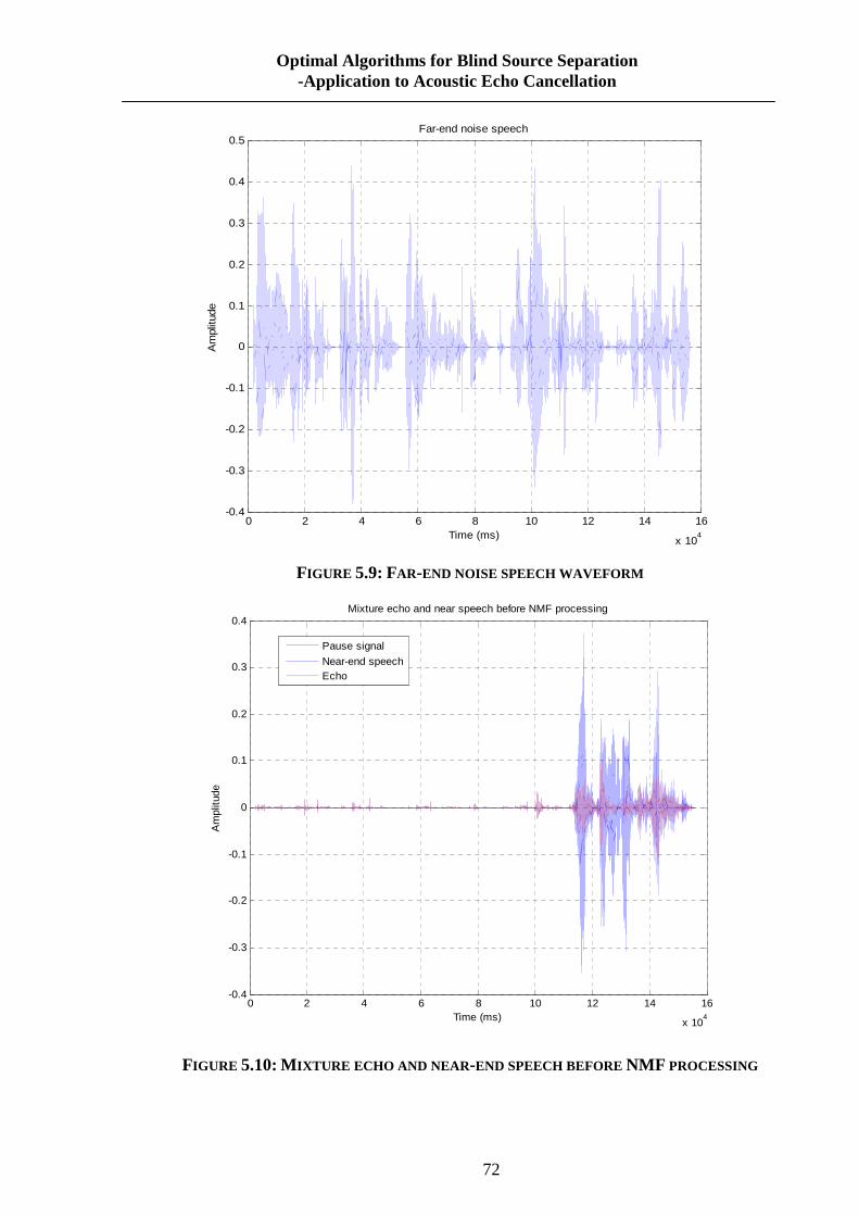
72


0 2 4 6 8 10 12 14 16

x 104

-0.4

-0.3

-0.2

-0.1

0

0.1

0.2

0.3

0.4

0.5

Time (ms)

Am

plitu

de

Far-end noise speech

FIGURE 5.9: FAR-END NOISE SPEECH WAVEFORM

0 2 4 6 8 10 12 14 16

x 104

-0.4

-0.3

-0.2

-0.1

0

0.1

0.2

0.3

0.4

Time (ms)

Am

plitu

de

Mixture echo and near speech before NMF processing

Pause signal

Near-end speechEcho

FIGURE 5.10: M IXTURE ECHO AND NEAR -END SPEECH BEFORE NMF PROCESSING

73


0 2 4 6 8 10 12 14 16

x 104

-0.4

-0.3

-0.2

-0.1

0

0.1

0.2

0.3

0.4

Time (ms)

Am

plitu

de

Mixture residual echo and near-end speech after NMF processing

Pause signal

Near-end speechResidual echo

FIGURE 5.11: M IXTURE ECHO AND NEAR -END SPEECH AFTER NMF PROCESSING

5.3.3 Convolutive NMF Simulation Results

The implementation of convolutive NMF to perform Acoustic Echo Cancellation is using

the similar frame work as the conventional NMF. The original NMF process the data

frame by frame, i.e. each training and matching procedure only process one frame of data.

The convolutive NMF uses a singleV matrix which covers t frames of data instead of

one. In each updated iteration, first only update( )tW and shift H for one frame for t

times, then uses the average value of ( )tW to updateH . That’s because update( )tW

andH for each t may result in a mistaken estimate of H with the update for t = T −1

dominating over others.

( )

ˆ ˆ, ( ) ( )

( ) 11

TtT

TT t

tt t

t

→

→

⋅ ⋅ = • = •⋅ ⋅

V VW H

V VH H W WW

H (5.28)

The process of convolutive NMF becomes:

• Read in a number of frames of mixture.

• Training near-end basis using convolutive NMF update function in Eq. 5.28.

• Training echo basis using convolutive NMF update function.

• Forming the mixture basis using near-end and echo basis.

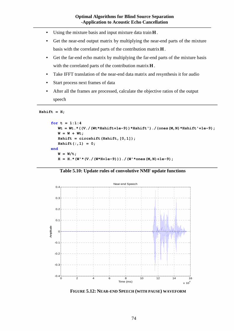
74


• Using the mixture basis and input mixture data trainH .

• Get the near-end output matrix by multiplying the near-end parts of the mixture

basis with the correlated parts of the contribution matrixH .

• Get the far-end echo matrix by multiplying the far-end parts of the mixture basis

with the correlated parts of the contribution matrix H .

• Take IFFT translation of the near-end data matrix and resynthesis it for audio

• Start process next frames of data

• After all the frames are processed, calculate the objective ratios of the output

speech

Hshift = H;

for t = 1:1:4 Wt = Wt.*((V./(Wt*Hshift+1e-9))*Hshift')./( ones(M,N)*Hshift'+1e-9); W = W + Wt; Hshift = circshift(Hshift,[0,1]); Hshift(:,1) = 0; end W = W/t; H = H.*(W'*(V./(W*H+1e-9)))./(W'*ones(M,N)+ 1e-9);

Table 5.10: Update rules of convolutive NMF update functions

0 2 4 6 8 10 12 14 16

x 104

-0.4

-0.3

-0.2

-0.1

0

0.1

0.2

0.3

0.4Near-end Speech

Time (ms)

Am

plitu

de

FIGURE 5.12: NEAR-END SPEECH (WITH PAUSE ) WAVEFORM

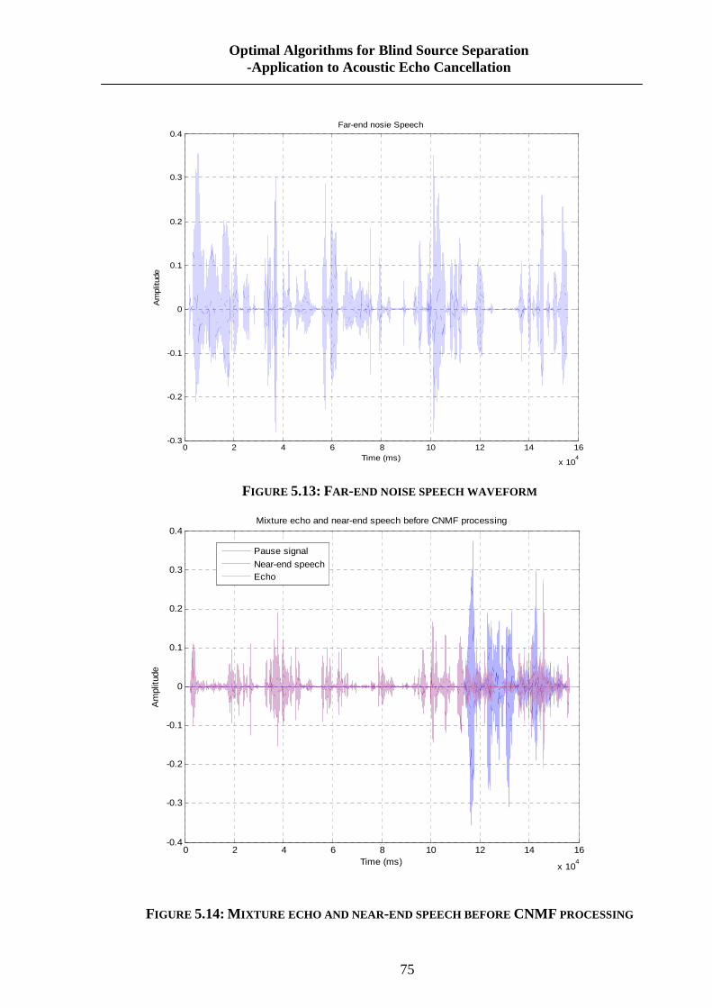
75


0 2 4 6 8 10 12 14 16

x 104

-0.3

-0.2

-0.1

0

0.1

0.2

0.3

0.4

Time (ms)

Am

plitu

de

Far-end nosie Speech

FIGURE 5.13: FAR-END NOISE SPEECH WAVEFORM

0 2 4 6 8 10 12 14 16

x 104

-0.4

-0.3

-0.2

-0.1

0

0.1

0.2

0.3

0.4

Time (ms)

Am

plitu

de

Mixture echo and near-end speech before CNMF processing

Pause signal

Near-end speechEcho

FIGURE 5.14: M IXTURE ECHO AND NEAR -END SPEECH BEFORE CNMF PROCESSING

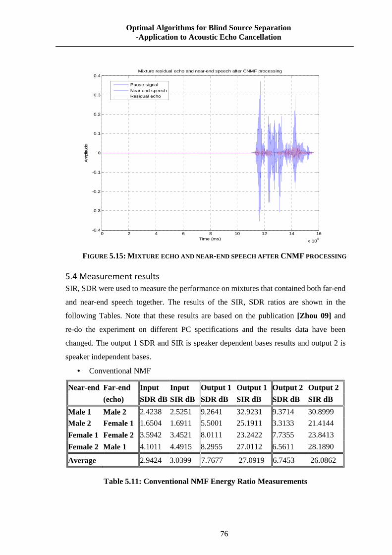
76


0 2 4 6 8 10 12 14 16

x 104

-0.4

-0.3

-0.2

-0.1

0

0.1

0.2

0.3

0.4

Time (ms)

Am

plitu

de

Mixture residual echo and near-end speech after CNMF processing

Pause signal

Near-end speechResidual echo

FIGURE 5.15: M IXTURE ECHO AND NEAR -END SPEECH AFTER CNMF PROCESSING

5.4 Measurement results

SIR, SDR were used to measure the performance on mixtures that contained both far-end

and near-end speech together. The results of the SIR, SDR ratios are shown in the

following Tables. Note that these results are based on the publication [Zhou 09] and

re-do the experiment on different PC specifications and the results data have been

changed. The output 1 SDR and SIR is speaker dependent bases results and output 2 is

speaker independent bases.

• Conventional NMF

Near-end Far-end Input Input Output 1 Output 1 Output 2 Outp ut 2

(echo) SDR dB SIR dB SDR dB SIR dB SDR dB SIR dB

Male 1 Male 2 2.4238 2.5251 9.2641 32.9231 9.3714 30.8999

Male 2 Female 1 1.6504 1.6911 5.5001 25.1911 3.3133 21.4144

Female 1 Female 2 3.5942 3.4521 8.0111 23.2422 7.7355 23.8413

Female 2 Male 1 4.1011 4.4915 8.2955 27.0112 6.5611 28.1890

Average 2.9424 3.0399 7.7677 27.0919 6.7453 26.0862

Table 5.11: Conventional NMF Energy Ratio Measurements

77


Near-end Far-end (echo) ERLE (dB)

Male 1 Male 2 12.1555 Male 2 Female 1 14.3672 Female 1 Female 2 12.6888 Female 2 Male 1 12.0794

Average 12.8227

Table 5.12: ERLE for pauses in near end speech (Conventional NMF)

• Convolutive NMF

Near-end Far-end Input Input Output 1 Output 1 Output 2 Outp ut 2

(echo) SDR dB SIR dB SDR dB SIR dB SDR dB SIR dB

Male 1 Male 2 3.0112 2.9385 9.2113 28.2301 9.0012 27.8999

Male 2 Female 1 3.2988 3.3111 6.4223 24.1247 6.7781 23.4144

Female 1 Female 2 2.6154 2.5908 8.7100 21.4450 7.5644 21.8413

Female 2 Male 1 3.0881 2.6557 5.5221 18.0047 5.1229 18.1890

Average 3.0036 2.8740 7.4664 22.9511 7.0067 22.8362

Table 5.13: Convolutive NMF Energy Ratio Measurements

Near-end Far-end (echo) ERLE (dB)

Male 1 Male 2 10.5442 Male 2 Female 1 12.1142 Female 1 Female 2 11.0012 Female 2 Male 1 9.9912

Average 10.9127

Table 5.14: ERLE for pauses in near end speech (Convolutive NMF)

5.5 Discussion and conclusions

In the above both NMF and CNMF simulation experiments, we use the randomly

chosen speakers to form the mixtures, two male and two female speeches (Chosen from

the TIMIT database). Each experimental mixture had a near end speaker contribution

and a far end speaker contribution. From the results of the figures in section 5.3, we can

find that both conventional NMF and convolutive NMF can give significant reduction

(approximate 8 to10% see figure 5.10, 5.11 and 5.15) in the level of echo. Note that the

convolutive NMF approach has trade-off between computational load and the level of

echo cancellation. In other words, in CNMF to cover more frames in one mixture gives

a more precise result or less residual echo, but it will leads to more computational load.

78


Therefore, in the experiment we found that processing eight frames can give a best

balance between algorithms computational load. The results showed that the

convolutive NMF approach gives comparable performance to the conventional NMF

but not better. However, as mentioned in chapter 4 if we improve the initialization

problem instead of randomly choosing the initial value, then both NMF algorithms can

achieve better performance.

The widely used methods are based on different types of Least Mean Squares (LMS)

algorithms. And these methods all have limitations in different aspects. Recent research

[Paul 07] [Cahill 08] [Zhou 09] also revealed that acoustic echo cancellation can also be

performed by employing a monaural sound source separation technique based on

Non-Negative Matrix Factorization (NMF), and significant echo suppression can be

achieved using this method, so using NMF approaches there are a few advantages over

the LMS algorithm.

Firstly, consider the effect reverberation has on theH matrix from NMF decompositions of

audio spectrograms. The rows ofH contain a time varying gain for each basis inW which

contains the contribution the basis makes to the mixture over time. TheH matrix is

normally a sparse matrix with activations occurring in single spikes for anechoic speech.

However in echoic version, if the sameW matrix was used the activations inH become

smeared. This is because the echoes in the speech manifest as repeated and smeared copies

of the anechoic spectrogram. The NMF represents these echoes as repeated and scaled

copies of the originalW basis over time. This property of the NMF audio spectrogram

enables the basis to be trained on anechoic speech and then can be used to separate echoic

speech. This applies to AEC as the reference signal first excites a LEM system before

reaching the microphone.

Secondly, the effect of misdjustments is reduced. The NMF does not estimate the LEM

filter thus it does not require further samples of the reference signal to converge to the new

room response like LMS, instead, it continuously adapts to the data present in the speech

signal. This also means that the length of the impulse response is insignificant, as NMF will

use the best available bases (the reference signal basis) to match the contribution from long

impulse responses. In the case of long LEM filters the LMS techniques usually fix the

length of the estimation filters.

79


Lastly using this approach Doubletalk will have less effect on this system, as this approach

uses a local speaker basis to match any near end speech [Cahill 08].

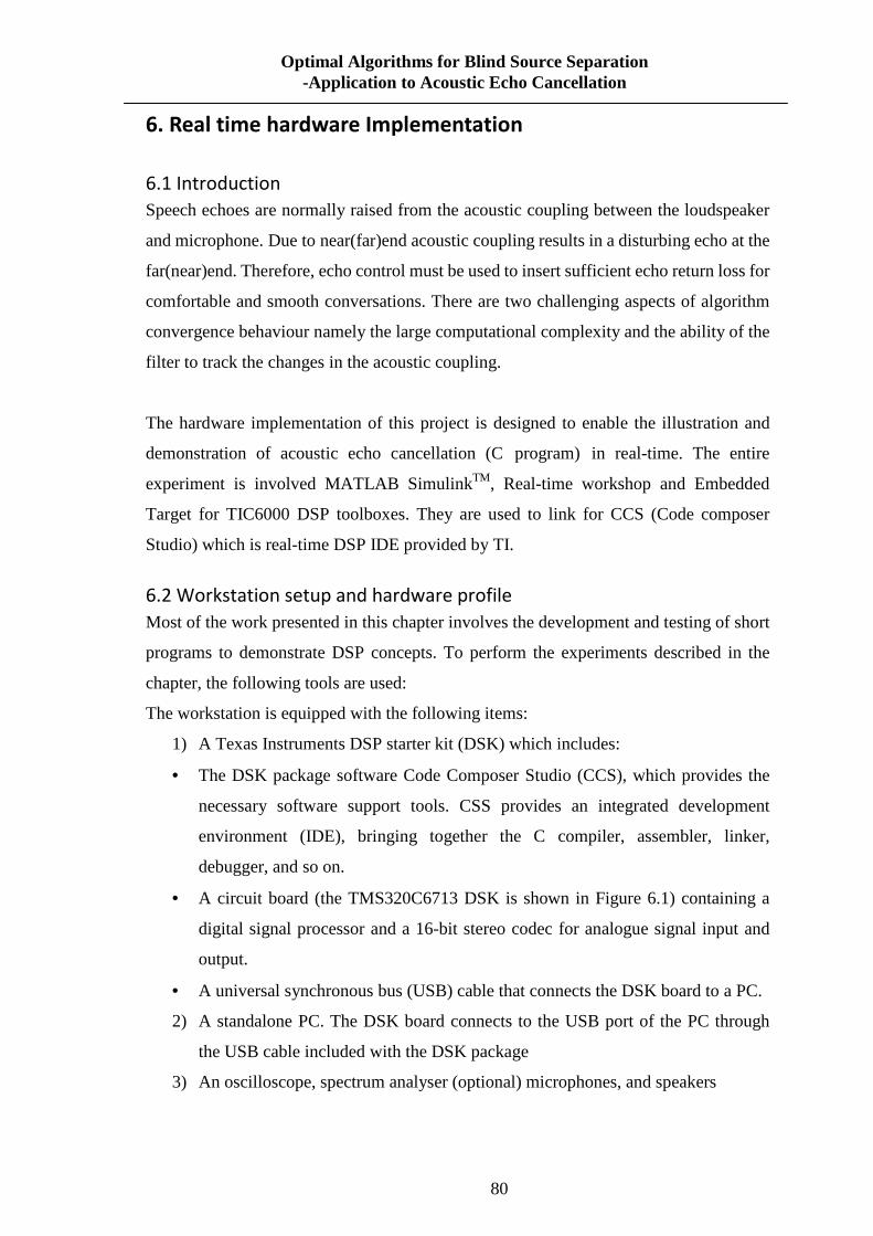
80


6. Real time hardware Implementation

6.1 Introduction

Speech echoes are normally raised from the acoustic coupling between the loudspeaker

and microphone. Due to near(far)end acoustic coupling results in a disturbing echo at the

far(near)end. Therefore, echo control must be used to insert sufficient echo return loss for

comfortable and smooth conversations. There are two challenging aspects of algorithm

convergence behaviour namely the large computational complexity and the ability of the

filter to track the changes in the acoustic coupling.

The hardware implementation of this project is designed to enable the illustration and

demonstration of acoustic echo cancellation (C program) in real-time. The entire

experiment is involved MATLAB SimulinkTM, Real-time workshop and Embedded

Target for TIC6000 DSP toolboxes. They are used to link for CCS (Code composer

Studio) which is real-time DSP IDE provided by TI.

6.2 Workstation setup and hardware profile

Most of the work presented in this chapter involves the development and testing of short

programs to demonstrate DSP concepts. To perform the experiments described in the

chapter, the following tools are used:

The workstation is equipped with the following items:

1) A Texas Instruments DSP starter kit (DSK) which includes:

• The DSK package software Code Composer Studio (CCS), which provides the

necessary software support tools. CSS provides an integrated development

environment (IDE), bringing together the C compiler, assembler, linker,

debugger, and so on.

• A circuit board (the TMS320C6713 DSK is shown in Figure 6.1) containing a

digital signal processor and a 16-bit stereo codec for analogue signal input and

output.

• A universal synchronous bus (USB) cable that connects the DSK board to a PC.

2) A standalone PC. The DSK board connects to the USB port of the PC through

the USB cable included with the DSK package

3) An oscilloscope, spectrum analyser (optional) microphones, and speakers

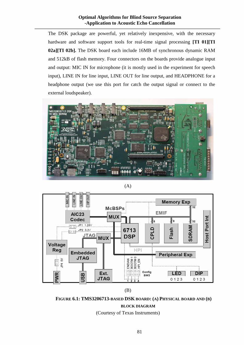
81


The DSK package are powerful, yet relatively inexpensive, with the necessary

hardware and software support tools for real-time signal processing [TI 01][TI

02a][TI 02b]. The DSK board each include 16MB of synchronous dynamic RAM

and 512kB of flash memory. Four connectors on the boards provide analogue input

and output: MIC IN for microphone (it is mostly used in the experiment for speech

input), LINE IN for line input, LINE OUT for line output, and HEADPHONE for a

headphone output (we use this port for catch the output signal or connect to the

external loudspeaker).

(A)

(B)

FIGURE 6.1: TMS3206713-BASED DSK BOARD: (A) PHYSICAL BOARD AND (B) BLOCK DIAGRAM

(Courtesy of Texas Instruments)

82


The DSK C6713 evaluation board installed within a simple enclosure which consists of

top and bottom precision machined transparent Plexiglas panels, those are then fastened

through the DSK board.

6.3 Real-time application setup

6.3.1 RTDX Technology

Real-Time Data Exchange (RTDXTM) is a technology developed by Texas Instruments

that provides effective real-time bi-directional communication between a digital signal

processor (DSP) or microcontroller and a host application in other words, it allows

system developers to transfer data between a host computer (MATLAB) and targets

device (C6713 DSK) without interfering with the target application[TI 01] . This

bi-directional communication path provides for data collection by the host as well as

host interaction with the running target application. RTDX also enables host systems to

provide data stimulation to the target application and algorithms [Dustin 02a].

6.3.2 RTDX Link to MATLAB

In this experiment, we illustrated the interface between MATLAB and the DSK using

RTDX. A buffer of data (i.e. speech wave file) created from MATLAB which running

on the host PC is set to the C6713 processor. The C source program running on the

DSK increment each data value in the buffer and sends the buffer of data back to

MATLAB. In other words, it creates two channels through RTDX: an input channel to

transfer data from MATLAB on the PC to the c6713 processor on the DSK and an

output channel to transfer data from the target DSK to the PC host. When the input

channel is enabled data are read or received as input to the DSK from MATLAB. After

each data value in the buffer is incremented by 1, an output channel is enabled to write

the data to MATLAB. Note that the input and output designations are from target DSK.

There are real-time application literatures [Dustin 02][Dustin 03][Horst 05][Fu 02]

discussed the RTDX technology throughout TI DSK project.

6.4 Speech recognition Implementation

Speech recognition refers to the concept of recognizing a speaker by his/her voice or

speech sample. Simply said speech recognition systems contain two main modules:

feature extraction and classification.

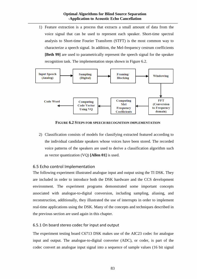
83


1) Feature extraction is a process that extracts a small amount of data from the

voice signal that can be used to represent each speaker. Short-time spectral

analysis to Short-time Fourier Transform (STFT) is the most common way to

characterize a speech signal. In addition, the Mel-frequency cestrum coefficients

[Beth 99] are used to parametrically represent the speech signal for the speaker

recognition task. The implementation steps shown in Figure 6.2.

FIGURE 6.2 STEPS FOR SPEECH RECOGNITION IMPLEMENTATION

2) Classification consists of models for classifying extracted featured according to

the individual candidate speakers whose voices have been stored. The recorded

voice patterns of the speakers are used to derive a classification algorithm such

as vector quantization (VQ) [Allen 01] is used.

6.5 Echo control Implementation

The following experiment illustrated analogue input and output using the TI DSK. They

are included in order to introduce both the DSK hardware and the CCS development

environment. The experiment programs demonstrated some important concepts

associated with analogue-to-digital conversion, including sampling, aliasing, and

reconstruction, additionally, they illustrated the use of interrupts in order to implement

real-time applications using the DSK. Many of the concepts and techniques described in

the previous section are used again in this chapter.

6.5.1 On board stereo codec for input and output

The experiment testing board C6713 DSK makes use of the AIC23 codec for analogue

input and output. The analogue-to-digital converter (ADC), or coder, is part of the

codec convert an analogue input signal into a sequence of sample values (16 bit signal

84


integer) to be processed by the digital signal processor (DSP). The digital-to-analogue

converter (DAC), or decoder, is part of the codec reconstructs an analogue output signal

from a sequence of sample value that have been processed by the DSP as well.

The AIC23 is a stereo audio codec based on sigma-delta technology [Norsworthy

97][Aziz 96][Candy 92]. Communication with the AIC23 codec for input and output

uses two multi-channel buffered serial ports (McBSPs) on the C6713. McBSP0 is used

as a unidirectional channel to send 16-bit control word to the AIC23. McBSP1 is used

as a bidirectional channel to send and receive audio data. The codec can be configured

for data-transfer word lengths of 16 up to 32 bits.

In the experiment, we need to define DSK support files which can initialize the DSK.

All the source files are written in C program. The following functions defined in support

file and explained for testing purposes:

Main c programme support file 6.1: c6713dskinit.c

Uint16 inputsource = DSK6713_AIC23_INPUT_MIC; // select input void main( ) { short sample_data; // in this case we choose select real-time speech input com_poll( ); // initialize DSK, codec, McBSP while(1) {

sample_data = input_left_sample( ) // input sample output_left_sample(sample_data); //output sample

} }

Table 6.1: Loop program using polling Above C source file for a program, which simply copies input samples read from the

AIC23 codec ADC back to the AIC23 codec DAC as output samples is listed in table

6.1. Effectively, the MIC input socket is connected straight through to the

HEADPHONE OUT socket on the DSK via the AIC23 codec and the digital signal

processor.

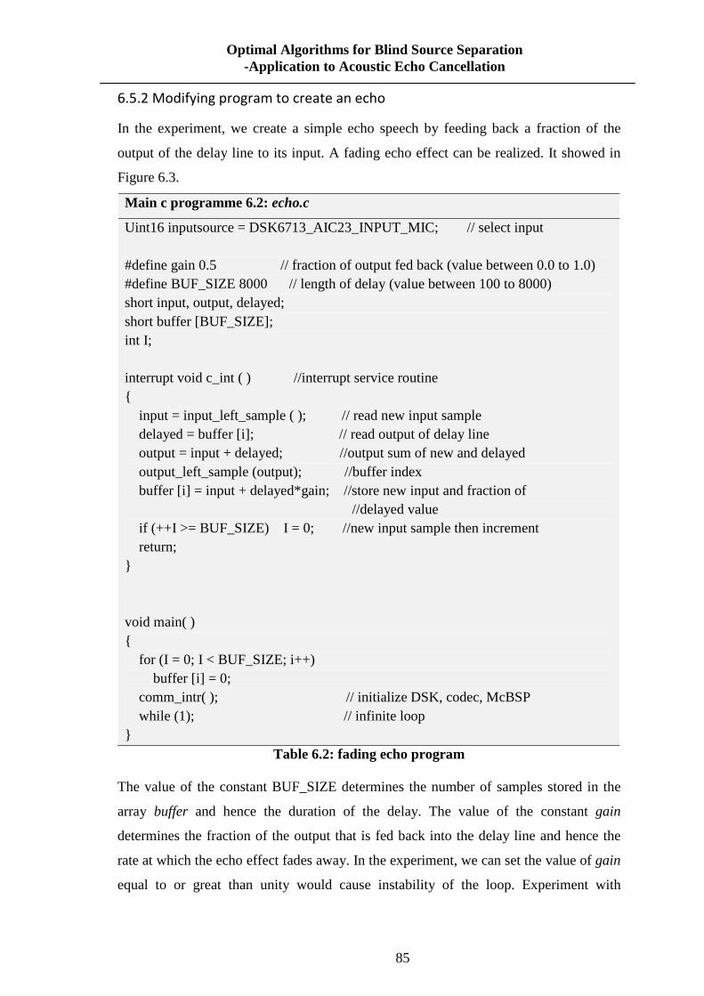
85


6.5.2 Modifying program to create an echo

In the experiment, we create a simple echo speech by feeding back a fraction of the

output of the delay line to its input. A fading echo effect can be realized. It showed in

Figure 6.3.

Main c programme 6.2: echo.c

Uint16 inputsource = DSK6713_AIC23_INPUT_MIC; // select input #define gain 0.5 // fraction of output fed back (value between 0.0 to 1.0) #define BUF_SIZE 8000 // length of delay (value between 100 to 8000) short input, output, delayed; short buffer [BUF_SIZE]; int I; interrupt void c_int ( ) //interrupt service routine { input = input_left_sample ( ); // read new input sample delayed = buffer [i]; // read output of delay line output = input + delayed; //output sum of new and delayed output_left_sample (output); //buffer index buffer [i] = input + delayed*gain; //store new input and fraction of //delayed value if (++I >= BUF_SIZE) I = 0; //new input sample then increment return; } void main( ) { for (I = 0; I < BUF_SIZE; i++)

buffer [i] = 0; comm_intr( ); // initialize DSK, codec, McBSP while (1); // infinite loop }

Table 6.2: fading echo program

The value of the constant BUF_SIZE determines the number of samples stored in the

array buffer and hence the duration of the delay. The value of the constant gain

determines the fraction of the output that is fed back into the delay line and hence the

rate at which the echo effect fades away. In the experiment, we can set the value of gain

equal to or great than unity would cause instability of the loop. Experiment with

86


different values of gain can be set as between 0 and 1 with 0.1 increment and

BUF_SIZE can be set as between 100 and 8000 with 1 increment.

FIGURE 6.3: SIMPLE BLOCK DIAGRAM REPRESENTION OF FADING ECHO PROGRAM

6.5.3 Modifying program to create an echo control

In the experiment we will extend the fading echo program to allow real-time adjustment

of gain and delay parameters of the echo effect.

Main c programme 6.3: echo_control.c

Uint16 inputsource = DSK6713_AIC23_INPUT_MIC; // select input #define MAX_BUF_SIZE 8000 //set maximum length of delay float gain = 0.5; short buflength = 1000; short buffer[MAX_BUF_SIZE]; //storage for previous samples short input, output, delayed; int I = 0; interrupt void c_int ( ) //interrupt service routine { input = input_left_sample ( ); // read new input sample delayed = buffer [i]; // read output of delay line output = input + delayed; //output sum of new and delayed output_left_sample (output); //buffer index buffer [i] = input + delayed*gain ; //store new input and fraction of //delayed value if (++I >= MAX_BUF_SIZE) //new input sample then increment

I = MAX_BUF_SIZE – buflength; return; }

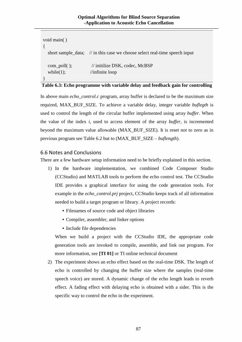
87


void main( ) { short sample_data; // in this case we choose select real-time speech input com_poll( ); // initilize DSK, codec, McBSP while(1); //infinite loop } Table 6.3: Echo programme with variable delay and feedback gain for controlling

In above main echo_control.c program, array buffer is declared to be the maximum size

required, MAX_BUF_SIZE. To achieve a variable delay, integer variable buflegth is

used to control the length of the circular buffer implemented using array buffer. When

the value of the index i, used to access element of the array buffer, is incremented

beyond the maximum value allowable (MAX_BUF_SIZE). It is reset not to zero as in

previous program see Table 6.2 but to (MAX_BUF_SIZE – buflength).

6.6 Notes and Conclusions

There are a few hardware setup information need to be briefly explained in this section.

1) In the hardware implementation, we combined Code Composer Studio

(CCStudio) and MATLAB tools to perform the echo control test. The CCStudio

IDE provides a graphical interface for using the code generation tools. For

example in the echo_control.prj project, CCStudio keeps track of all information

needed to build a target program or library. A project records:

• Filenames of source code and object libraries

• Compiler, assembler, and linker options

• Include file dependencies

When we build a project with the CCStudio IDE, the appropriate code

generation tools are invoked to compile, assemble, and link out program. For

more information, see [TI 01] or TI online technical document

2) The experiment shows an echo effect based on the real-time DSK. The length of

echo is controlled by changing the buffer size where the samples (real-time

speech voice) are stored. A dynamic change of the echo length leads to reverb

effect. A fading effect with delaying echo is obtained with a sider. This is the

specific way to control the echo in the experiment.

88


7. Conclusion and future work

An extensive review of optimum algorithms for blind source separation was presented,

as well as a review of Non-negative Matrix Factorization (NMF) and Least Mean

Square (LMS) based approaches. Based on these reviews it was concluded that using

different mathematical techniques to perform Acoustic Echo Cancellation (AEC), by

comparing results and considering the trade-off issues we can find the best suitable

algorithm for the AEC problem.

This thesis demonstrated two research sub-topics for AEC: the first employs different

versions of Least Mean Square algorithms to perform acoustic echo cancellation, we use

a dataset from real-time echo speech which is collected TI C6713 DSK. By comparing

the ERLE value, we can find best suitable version of LMS algorithm which we

discussed in the experiment; the second topic presented a new technique called

convolutive non-negative matrix factorization to perform acoustic echo cancellation.

The two NMF experiments were implemented in MATLAB environment by using the

same dataset of input speeches, performing the steps of training near-end and far-end

reference bases, forming mixture bases, using the reference bases separate the mixture

data, and finally resynthesis the required speech part in the mixture as the output speech.

Finally, the output speech is analysed by objective measures included SDR, SIR, ERIE

and the comparable analytic data shown as a table form. Although the experiments of

convolutive NMF showed the new algorithm didn’t give a better performance than

conventional version, this can help further research in modifying the algorithm or

combine the feature of different version of the algorithm to give better performance.

Also the last part, we present a simple real-time echo control implementation. It is based

on TI C6713 development start kit. The real-time scenario let us understand how to

create and control echo by modifying the c program function. Also use RTDX

Technology to connect MATLAB and DSK is another useful experimental experience.

7.1 Future work

Further work on the topic of Convolutive NMF includes combining features of different

versions of NMF such as Local NMF (LNMF) or other mathematical tools, find the

optimal or best suitable algorithm for different applications such as AEC, musical

89


separation, etc. Alternatively some of the non-linear post-processing techniques used to

improve LMS methods such as component zeroing could be employed to improve

performance [Virtanen 07].

The nonnegative matrix factorization has many advantages to alternative techniques for

processing such matrices, but it must be initialized and the initialization selected is

crucial to getting better solutions. It is an open issue [Amy 06] [Stefan 04] for NMF

algorithms research.

At present the algorithms described in this thesis are all implemented in MATLAB. A

useful area for the future work would be the implementation of these algorithms in C or

C++ which would result in a considerable reduction in the time required to run the

algorithms. Additionally, to implement the algorithms into real-time is also an important

future work. Hardware features such as computational load, delay and floating or fixed

point operation of the hardware can affects the performance of algorithms in the real-time

environment. Balancing and adjustment of the algorithm parameters are needed, translate

the algorithms into C orC++ is also required

In conclusion, the work undertaken has identified a number of possibilities for

improvement in acoustic echo cancellation approaches. The technique implementations

demonstrated using sound source separation algorithms such as NMF can be further

improved by employing more efficient cost functions. It is hoped that future work will

further enhance the thrust of this research.

Acknowledgements

This work is supported by Enterprise Ireland Commercialization Fund Technology

Development Grant (EI/CFTD/06/235).

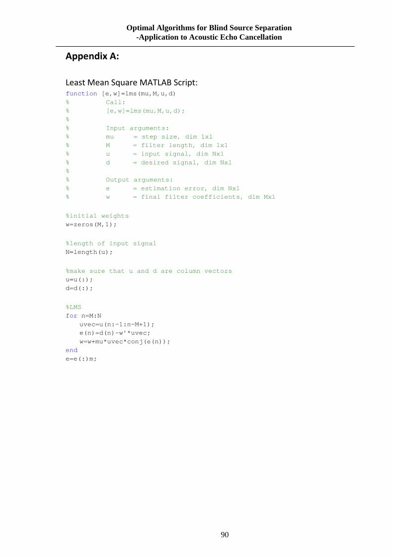
90


Appendix A:

Least Mean Square MATLAB Script: function [e,w]=lms(mu,M,u,d) % Call: % [e,w]=lms(mu,M,u,d); % % Input arguments: % mu = step size, dim 1x1 % M = filter length, dim 1x1 % u = input signal, dim Nx1 % d = desired signal, dim Nx1 % % Output arguments: % e = estimation error, dim Nx1 % w = final filter coefficients, di m Mx1 %initial weights w=zeros(M,1); %length of input signal N=length(u); %make sure that u and d are column vectors u=u(:); d=d(:); %LMS for n=M:N

uvec=u(n:-1:n-M+1); e(n)=d(n)-w’*uvec; w=w+mu*uvec*conj(e(n));

end e=e(:)m;

91


Normalized Least Mean Square MATLAB Script: function [e,w]=nlms(mu,M,u,d,a) % Normalized LMS % Call: % [e,w]=nlms(mu,M,u,d,a); % % Input arguments: % mu = step size, dim 1x1 % M = filter length, dim 1x1 % u = input signal, dim Nx1 % a = constant, dim 1x1 % % Output arguments: % e = estimation error, dim Nx1 % w = final filter coefficients, di m Mx1 %intial value 0 w=zeros(M,1); %input signal length N=length(u); %make sure that u and d are colon vectors u=u(:); d=d(:); %NLMS for n=M:N uvec=u(n:-1:n-M+1); e(n)=d(n)-w’*uvec; w=w+mu/(a+uvec’*uvec)*uvec*conj(e(n)); end

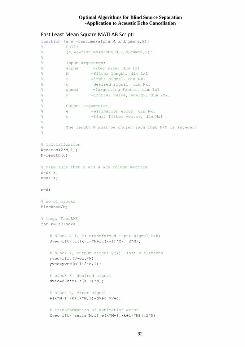
92


Fast Least Mean Square MATLAB Script: function [e,w]=fastlms(alpha,M,u,d,gamma,P); % Call: % [e,w]=fastlms(alpha,M,u,d,gamma,P); % % Input arguments: % alpha =step size, dim 1x1 % M =filter length, dim 1x1 % u =input signal, dim Nx1 % d =desired signal, dim Nx1 % gamma =forgetting factor, dim 1x1 % P =initial value, energy, dim 2Mx1 % % Output arguments: % e =estimation error, dim Nx1 % w =final filter vector, dim M x1 % % The length N must be chosen such that N /M is integer! % % initialization W=zeros(2*M,1); N=length(u); % make sure that d and u are column vectors d=d(:); u=u(:); e=d; % no.of blocks Blocks=N/M; % loop, FastLMS for k=1:Blocks-1

% block k-1, k; transformed input signal U(k) Uvec=fft([u((k-1)*M+1:(k+1)*M)],2*M);

% block k, output signal y(k), last M elements yvec=ifft(Uvec.*W); yvec=yvec(M+1:2*M,1);

% block k; desired signal dvec=d(k*M+1:(k+1)*M);

% block k, error signal e(k*M+1:(k+1)*M,1)=dvec-yvec;

% transformation of estimation error Evec=fft([zeros(M,1);e(k*M+1:(k+1)*M)],2*M);

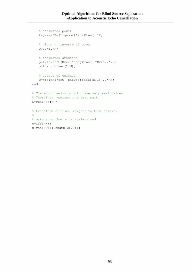
93


% estimated power P=gamma*P+(1-gamma)*abs(Uvec).^2;

% block k, inverse of power Dvec=1./P;

% estimated gradient phivec=ifft(Dvec.*conj(Uvec).*Evec,2*M); phivec=phivec(1:M);

% update of weights W=W+alpha*fft([phivec;zeros(M,1)],2*M);

end % The error vector should have only real values. % Therefore, extract the real part! E=real(e(:)); % transform of final weights to time domain. % % make sure that w is real-valued w=ifft(W); w=real(w(1:length(W)/2));

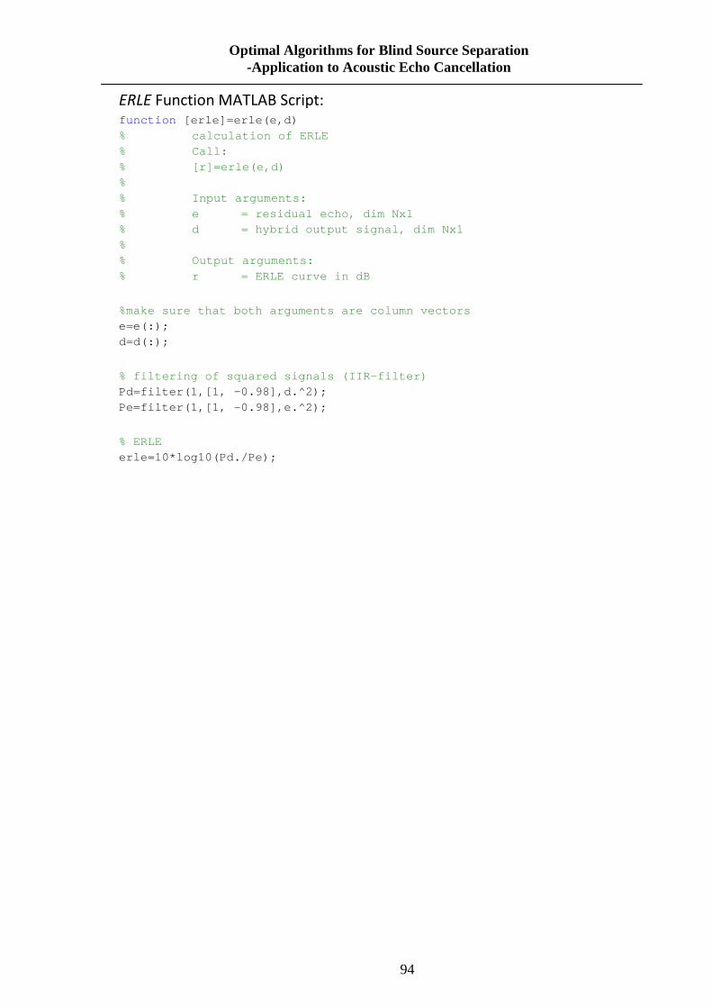
94


ERLE Function MATLAB Script: function [erle]=erle(e,d) % calculation of ERLE % Call: % [r]=erle(e,d) % % Input arguments: % e = residual echo, dim Nx1 % d = hybrid output signal, dim Nx1 % % Output arguments: % r = ERLE curve in dB %make sure that both arguments are column vectors e=e(:); d=d(:); % filtering of squared signals (IIR-filter) Pd=filter(1,[1, -0.98],d.^2); Pe=filter(1,[1, -0.98],e.^2); % ERLE erle=10*log10(Pd./Pe);

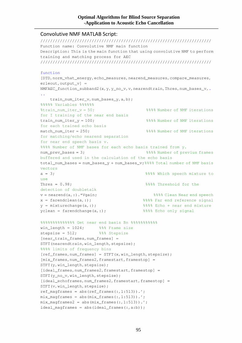
95


Convolutive NMF MATLAB Script: /////////////////////////////////////////////////// /////////////////// Function name: Convolutive NMF main function Description: This is the main function that using c onvolutive NMF to perform training and matching process for AEC /////////////////////////////////////////////////// /////////////////// function [DTD,norm_vhat_energy,echo_measures,nearend_measure s,compare_measures,erleout,output_v] = NMFAEC_function_subband2(x,y,y_no_v,v,nearendtrain, Thres,num_bases_v, ...

train_num_iter_v,num_bases_y,a,b); %%%%% Variables %%%%%% %train_num_iter_v = 50; %%%% Nu mber of NMF iterations for I training of the near end basis train_num_iter_y = 100; %%%% Number of NMF iterations for each trained echo basis match_num_iter = 250; %%%% Number of NMF iterations for matching/echo nearend separation for near end speech basis v. %%%% Number of NMF bases for each echo basis traine d from y. num_prev_bases = 3; %%%% Number of previus frames buffered and used in the calculation of the echo ba sis total_num_bases = num_bases_y + num_bases_v; %%%% Total number of NMF basis vectors a = 3; %%%% Which spe ech mixture to use Thres = 0.98; %%%% Threshold for th e detection of doubletalk v = nearend(a,:).*Vgain; %%%% Clean Near end speech x = farendclean(a,:); %%%% Far end reference signal y = mixturechange(a,:); %%%% Echo + near end mixture yclean = farendchange(a,:); %%%% Echo only signal %%%%%%%%%%%%%% Get near end basis Bn %%%%%%%%%%% win_length = 1024; %%% Frame size stepsize = 512; %%% Stepsize [near_train_frames,num_frames] = STFT(nearendtrain,win_length,stepsize); %%%% limits of frequency bins [ref_frames,num_frames] = STFT(x,win_length,stepsiz e); [mix_frames,num_frames2,framestart,framestop] = STFT(y,win_length,stepsize); [ideal_frames,num_frames2,framestart,framestop] = STFT(y_no_v,win_length,stepsize); [ideal_echoframes,num_frames2,framestart,framestop] = STFT(v,win_length,stepsize); ref_magframes = abs(ref_frames(:,1:513)).’; mix_magframes = abs(mix_frames(:,1:513)).’; mix_magframes2 = abs(mix_frames(:,1:513)).’; ideal_magframes = abs(ideal_frames(:,a:b));

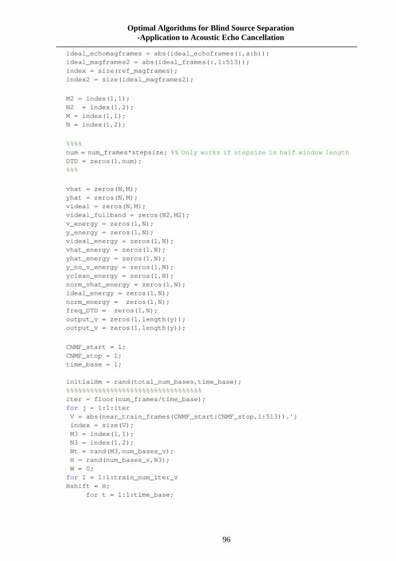
96


ideal_echomagframes = abs(ideal_echoframes(:,a:b)); ideal_magframes2 = abs(ideal_frames(:,1:513)); index = size(ref_magframes); index2 = size(ideal_magframes2); M2 = index(1,1); N2 = index(1,2); M = index(1,1); N = index(1,2); %%%% num = num_frames*stepsize; %% Only works if stepsize is half window length DTD = zeros(1,num); %%% vhat = zeros(N,M); yhat = zeros(N,M); videal = zeros(N,M); videal_fullband = zeros(N2,M2); v_energy = zeros(1,N); y_energy = zeros(1,N); videal_energy = zeros(1,N); vhat_energy = zeros(1,N); yhat_energy = zeros(1,N); y_no_v_energy = zeros(1,N); yclean_energy = zeros(1,N); norm_vhat_energy = zeros(1,N); ideal_energy = zeros(1,N); norm_energy = zeros(1,N); freq_DTD = zeros(1,N); output_v = zeros(1,length(y)); output_v = zeros(1,length(y)); CNMF_start = 1; CNMF_stop = 1; time_base = 1; initialHm = rand(total_num_bases,time_base); %%%%%%%%%%%%%%%%%%%%%%%%%%%%%%%%%% iter = floor(num_frames/time_base); for j = 1:1:iter V = abs(near_train_frames(CNMF_start:CNMF_stop,1:5 13)).’; index = size(V); M3 = index(1,1); N3 = index(1,2); Wt = rand(M3,num_bases_v); H = rand(num_bases_v,N3); W = 0; for I = 1:1:train_num_iter_v Hshift = H; for t = 1:1:time_base;

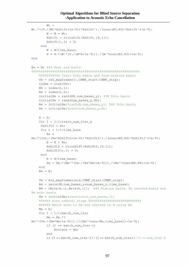
97


Wt = Wt.*((V./(Wt*Hshift+1e-9))*Hshift’)./(ones(M3,N3)*H shift’+1e-9); W = W + Wt; Hshift = circshift(Hshift,[0,1]); Hshift(:,1) = 0; end W = W/time_base; H = H.*(W’*(V./(W*H+1e-9)))./(W’*ones(M3,N3 )+1e-9); end Bn = W; %%% Near end basis %%%%%%%%%%%%%%%%%%%%%%%%%%%%%%%%%%%%%%%%%%%%%%%%%%%%%%%%%

%%%%%%%%%%% Train Echo basis and form mixture basis Ve = ref_magframes(:,CNMF_start:CNMF_stop); index = size(Ve); M4 = index(1,1); N4 = index(1,2); initialBe = rand(M4,num_bases_y); %%% Echo basis initialHe = rand(num_bases_y,N4); Be = initialBe; %rand(M,num_bases_y); %%% Echo basis He = initialHe; %rand(num_bases_y,N);

B = 0; for I = 1:1:train_num_iter_y

Hshift2 = He; for t = 1:1:time_base Be = Be.*((Ve./(Be*Hshift2+1e-9))*Hshift2’)./(ones(M4,N4 )*Hshift2’+1e-9); B = B + Be; Hshift2 = circshift(Hshift2,[0,1]); Hshift2(:,1) = 0; end B = B/time_base; He = He.*(Be’*(Ve./(Be*He+1e-9)))./(Be’*one s(M4,N4)+1e-9);

end Be = B;

Vm = mix_magframes(a:b,CNMF_start:CNMF_stop); Bm = zeros(M,num_bases_y+num_bases_v,time_base); Bm = [Bn(a:b,:),Be(a:b,:)]; %%% Mixture basis, Bn nearend basis and

Be echo basis Hm = initialHm; %rand(total_num_bases,1); %%%%%% Echo removal stage %%%%%%%%%%%%%%%%%%%%%%%%%%%% %%%%%% Match echo to Be and nearend to W using Bm Mx = b; for I = 1:1:match_num_iter

Hm = Hm.*( Bm’*(Vm./(Bm*Hm+1e-9)))./((Bm’*ones(Mx,time_base))+ 1e-9); if (I == match_num_iter-1) Hnolate = Hm; end if (I == match_num_iter-1)|(I == match_num_iter) %|(I == num_iter-2

98


Bm = Bm .*((Vm./(Bm *Hm+1e-9))*Hm’)./((ones(Mx,time_base)*Hm’)+1e-9); end

end mat_bot = [Bn(b+1:end,:),Be(b+1:end,:)]; Bm = [Bm;mat_bot]; vhat(CNMF_start:CNMF_stop,:) =

(Bm(:,1:total_num_bases-num_bases_y)*Hm(1:total_num _bases-num_bases_y,:)).’;

yhat(CNMF_start:CNMF_stop,:) = (Bm(:,num_bases_v+1:end)*Hm(num_bases_v+1:end,:)).’ ; CNMF_start = CNMF_start + time_base; CNMF_stop = CNMF_stop + time_base; end %%%% Resythesis for audio vhat = [vhat,fliplr(vhat(:,2:512))]; [xf,yf] = pol2cart(angle(mix_frames),vhat); resyn = complex(xf,yf); output_v = resynthesis(resyn,win_length,stepsize); %%%%%%%%%%%% Objective evaluation %%%%%%%%%%%%%%%%%% termin = length(output_v); org_sources = [v(107555:termin);y_no_v(107555:termi n)]; index = 1; [s_target,e_interf,e_artif] = bss_decomp_gain(outpu t_v(107555:termin), index, org_sources); [inputSDR,inputSIR,inputSAR] = bss_crit(s_target, e _interf, e_artif); nearend_measures = [inputSDR,inputSIR,inputSAR]; %%%%%%%% Resythesis no late W updates yhat = [yhat,fliplr(yhat(:,2:512))]; [xf,yf] = pol2cart(angle(mix_frames),yhat); resyn = complex(xf,yf); output_y = resynthesis(resyn,win_length,stepsize); %%%%%%%%%%%%%%%% org_sources = [y_no_v(107555:termin);v(107555:termi n)]; index = 1; [s_target,e_interf,e_artif] = bss_decomp_gain(outpu t_y(107555:termin), index, org_sources); [inputSDR,inputSIR,inputSAR] = bss_crit(s_target, e _interf, e_artif); echo_measures = [inputSDR,inputSIR,inputSAR]; %%%% Reconstruct with different phase [frames,num_frames] = STFT(v,win_length,stepsize); [framesnear,num_framesnear] = STFT(v,win_length,ste psize); [xf,yf] = pol2cart(angle(mix_frames),abs(framesnear )); resyn = complex(xf,yf); diffphasereconstruct = resynthesis(resyn,win_length ,stepsize); %%%%%%%%%%%%%%%%%%%%%%%%%%%%%%%% org_sources = [v(107555:termin);y_no_v(107555:termi n)]; index = 1;

99


[s_target,e_interf,e_artif] = bss_decomp_gain(diffphasereconstruct(107555:termin) , index, org_sources); [inputSDR,inputSIR,inputSAR] = bss_crit(s_target, e _interf, e_artif); compare_measures = [inputSDR,inputSIR,inputSAR]; %%%%%%%%%%%%%%%%%%%%%%%%%%%%%%%%%%% erleout = ERLE(y_no_v,output_v,win_length,stepsize) ; %%%%%%%%%% figure plot(real(output_v)) figure plot(real(output_y)) figure plot(v) grid on;

hold plot(DTD, ’r’ ) grid on;

figure plot(vhat_energy) grid on; hold

plot(freq_DTD* 0.3, ’r’ ) grid on; figure

plot(v) hold grid on; plot(real(output_v)) plot(real(output_v) – v(1:length(output_v)), ’k’ )

figure plot(v) grid on;

hold plot(diffphasereconstruct) plot(diffphasereconstruct – v(1:length(output_v)), ’k’ ) grid on;

100


Objective Measure MATLAB Script: /////////////////////////////////////////////////// /////////////// Function Name: Objective measure function Description: compute evaluation criteria given a de composition of an estimated source into target/interference/noise/art ifacts of the form se = s_target + e_interf (+ e_noise) + e_artif Developers: - Cedric Fevotte ([email protected]) – E mmanuel Vincent ( [email protected]) – Remi Gribonval ( [email protected] ) /////////////////////////////////////////////////// /////////////// % Usage: % % 1) Global mode % % [SDR,SIR,(SNR,)SAR]=bss_crit(s_target,e_interf[,e _noise],e_artif) % % Input: % - s_target: row vector of length T containing t he target source(s) % contribution, % - e_interf: row vector of length T containing t he interferences % contribution, % - e_noise: row vector of length T containing th e noise contribution % (if any), % - e_artif: row vector of length T containing th e artifacts % contribution. % % Output: % - SDR: Source to Distortion Ratio, % - SIR: Source to Interferences Ratio, % - SNR: Signal to Noise Ratio (if e_noise is pro vided), % - SAR: Source to Artifacts Ratio. % % 2) Local mode % % [SDR,SIR,(SNR,)SAR]=bss_crit(s_target,e_interf[,e_n oise],e_artif,WINDOW,NOVERLAP) % % Additional input: % - WINDOW: 1 x W window % - NOVERLAP: number of samples of overlap betwee n consecutive windows % % Output: % - SDR: n_frames x 1 vector containing local Sou rce to Distortion Ratio, % - SIR: n_frames x 1 vector containing local Sou rce to Interferences Ratio, % - SNR: n_frames x 1 vector containing local Sig nal to Noise Ratio, % - SAR: n_frames x 1 vector containing local Sou rce to Artifacts Ratio. % % Developers: - Cedric Fevotte ([email protected]) – Emmanuel Vincent % ( [email protected]) – Remi Gribonval ( [email protected] )

101


function varargout=bss_crit(varargin) s_target=varargin{1}; e_interf=varargin{2}; switch nargin

case 3 e_noise=[]; e_artif=varargin{3}; mode= ’global’ ;

case 4 e_noise=varargin{3}; e_artif=varargin{4}; mode= ’global’ ;

case 5 e_noise=[]; e_artif=varargin{3}; WINDOW=varargin{4}; NOVERLAP=varargin{5}; mode= ’local’ ;

case 6 e_noise=varargin{3}; e_artif=varargin{4}; WINDOW=varargin{5}; NOVERLAP=varargin{6}; mode= ’local’ ; end T=length(s_target); switch mode

case ‘global’ switch isempty(e_noise) case 1 % Computation of the energy ratios [SDR,SIR,SAR]=bss_energy_ratios(s_target,e_interf,e _artif); varargout{1}=10*log10(SDR); varargo ut{2}=10*log10(SIR); varargout{3}=10*log10(SAR); case 0 % Computation of the energy ratios [SDR,SIR,SNR,SAR]=bss_energy_ratios(s_target,e_inte rf,e_noise,e_artif); varargout{1}=10*log10(SDR); varargo ut{2}=10*log10(SIR); varargout{3}=10*log10(SNR); varargout{4}=10*log10(S AR); end

case ‘local’ W=length(WINDOW); % Length of window n_frames = fix((T-NOVERLAP)/(W-NOVERLAP)); % Number of frames switch isempty(e_noise) case 1 F_s_target=bss_make_frames(s_target ,WINDOW,NOVERLAP); F_e_interf=bss_make_frames(e_interf ,WINDOW,NOVERLAP); F_e_artif=bss_make_frames(e_artif,W INDOW,NOVERLAP); [SDR,SIR,SAR]=bss_energy_ratios(F_s_target,F_e_inte rf,F_e_artif);

102


varargout{1}=10*log10(SDR); varargo ut{2}=10*log10(SIR); varargout{3}=10*log10(SAR); case 0 F_s_target=bss_make_frames(s_target ,WINDOW,NOVERLAP); F_e_interf=bss_make_frames(e_interf ,WINDOW,NOVERLAP); F_e_noise=bss_make_frames(e_noise,W INDOW,NOVERLAP); F_e_artif=bss_make_frames(e_artif,W INDOW,NOVERLAP); [SDR,SIR,SNR,SAR]=bss_energy_ratios(F_s_target,F_e_ interf,F_e_noise,F_e_artif); varargout{1}=10*log10(SDR); varargo ut{2}=10*log10(SIR); varargout{3}=10*log10(SNR); varargo ut{4}=10*log10(SAR); end end %mode

103


Resynthesis MATLAB Script: /////////////////////////////////////////////////// /////////////////// Function name: Resynthesis function Description: To rebuild the audible output speech f rom the matched data /////////////////////////////////////////////////// /////////////////// %%%%%%%%%%%%%%%% STFT resynthesis %%%%%%%%%%%%%%%%%%%%%%%%%%%%%%%%%%% function reconstruct = resynthesis(spec,win_length,stepsize ) dim = size(spec); num_frames = dim(1,1); N = dim(1,2); num_samples = num_frames*stepsize; reconstruct = zeros(1,num_samples); ham_win = hanning(win_length); start = 1; stop = win_length; for I = 1:1:num_frames

reconstruct(start:stop) = real(ifft(spec(I,:))) + reconstruct(start:stop);

start = start + stepsize; stop = stop + stepsize; if stop > num_samples

break end

end

104


Appendix B:

TI C6713 DSK Main C Program Implementation

echo.c echo with fixed delay and feedback

#include “DSK6713_AIC23.h” // codec support Uint32 fs=DSK6713_AIC23_FREQ_8KHZ; // set sampling rate #define DSK6713_AIC23_INPUT_MIC 0x0015 #define DSK6713_AIC23_INPUT_LINE 0x0011 Uint16 inputsource=DSK6713_AIC23_INPUT_MIC; // select input #define GAIN 0.6 // fraction (0 – 1) of output fed back #define BUF_SIZE 2000 // this sets length of delay short buffer[BUF_SIZE]; // storage for previous samples short input,output,delayed; int I; // index into buffer interrupt void c_int11() // interrupt service routine { input = input_left_sample(); // read new input sample from ADC delayed = buffer[i]; // read delayed value from buffer output = input + delayed; // output sum of input and delayed values output_left_sample(output); buffer[i] = input + delayed*GAIN; // store new input and a fraction // of the delayed value in buffer if(++I >= BUF_SIZE) i=0; // test for end of buffer return; // return from ISR } void main() { comm_intr(); // init DSK, codec, McBSP for(i=0 ; i<BUF_SIZE ; i++) // clear buffer

buffer[i] = 0; while(1); //infinite loop }

105


echo_control.c echo with variable delay and feedback

#include “DSK6713_AIC23.h” // codec support Uint32 fs=DSK6713_AIC23_FREQ_8KHZ; // set sampling rate #define DSK6713_AIC23_INPUT_MIC 0x0015 #define DSK6713_AIC23_INPUT_LINE 0x0011 Uint16 inputsource=DSK6713_AIC23_INPUT_MIC; // select input #define MAX_BUF_SIZE 8000 // this sets maximum length of delay float gain = 0.5; short buflength = 1000; short buffer[MAX_BUF_SIZE]; // storage for previous samples short input,output,delayed; int I = 0; // index into buffer interrupt void c_int11() // interrupt service routine { input = input_left_sample(); // read new input sample from ADC delayed = buffer[i]; // read delayed value from buffer output = input + delayed; // output sum of input and delayed values output_left_sample(output); buffer[i] = input + delayed*gain; // store new input and a fraction // of the delayed value in buffer if(++I >= MAX_BUF_SIZE) // test for end of buffer

I = MAX_BUF_SIZE – buflength; return; // return from ISR } void main() { for(i=0 ; i<MAX_BUF_SIZE ; i++) // clear buffer

buffer[i] = 0; comm_intr(); // init DSK, codec, McBSP while(1); //infinite loop }

106


Bibliography

[Allen 01] Allen G. and Robert M. G., “Vector Quantization and signal

Compression”, pp309-317, Kluwer Academic Publishers, 2001

[Amy 06] Amy N. Carl D. Russell A., “Initializations for the Nonnegative

Matrix Factorization”, Department of Mathematics College of

Charleston, 2006.

[Aziz 96] Aziz P.M., Sorensen H.V., and Van Der Spiegel J., “An overview of

sigma delta converters”, IEEE Signal Processing, Jan, 1996.

[Barry 04a] Barry D., Lawlor B., Coyle E. “Sound Source Separation: Azimuth

Discrimination and Resynthesis” Proc of the 7th International

Conference on Digital Audio Effect (DAFX-04) Naples, Italy,

October 5-8, 2004.

[Barry 04b] Barry D. (2004) “Sound Source Separation” Transfer Report 2004,

pp36.

[Barry 04c] Barry D. (2004) “Sound Source Separation” Transfer Report 2004,

pp41-42.

[Baeza 92] Baeza-Yates R.A.. “Introduction to data structures and algorithms

related to information retrieval”. In information Retrieval: Data

Structures and Algorithms, pages 13-27. Prentice-Hall, Inc., Upper

Saddle River, NJ, USA, 1992.

[Bell 05] Bell A.J. and T.J. Sejnowski, “An information maximization

approach to blind separation and blind deconvolution”, Neural

Computation, 7: 1 129-1 159, 1995

[Bertsekas 99] Bertsekas D., “Nonlinear programming”, Athena Scientific,

Belmont, MA, 1999

[Beth 99] Beth L., “Mel Frequency Cepstral Coefficients for Music

Modelling”, Cambridge Research Laboratory Compaq Computer

Corporation, 1999.

[Bofill 03] Bofill P.. Underdetermined blind source separation of delayed sound

sources in the frequency domain. Neurocomputing, 55(1):627–641,

2003.

[Broman 99] Broman H., Lindgren U., Sahlin H., and Stoica P., “Source

separation: A TITO system identification approach”, Signal

107


Processing, 73:169-183, 1999

[Bronkhorst 00] Bronkhorst, Adelbert W. (2000). “The Cocktail Party Phenomenon:

A Review on Speech Intelligibility in Multiple-Talker

Conditions” . Acta Acustica united with Acustica 86: 117–128, 2000

[Cahill 06] Cahill N. “Sound Source Separation and Speech Enhancement using

a Modified ADRess Algorithm with application in Mobile

Communication”, pp18, M.Eng. Sc. Thesis, NUI Maynooth, Oct.

2006

[Cahill 08] Niall Cahill and Robert Lawlor. “A novel Approach to Acoustic Echo

Cancellation", 16th European Signal Processing Conference, 2008

[Candy 92] Candy J.C. and Temes G.C., Eds., “Oversampling Delta-Sigma Data

Converters: Theory, Design and Simulation”, IEEE Press,

Piscataway, NJ, 1992.

[Cardoso 89] Cardoso J.-F.. Source separation using higher-order moments. In

Proc. IEEE Int. Conf. Acoustics, Speech, Signal Processing

(ICASSP), volume 4, pages 2109–2112, lasgow, Scotland, May

1989.

[Cardoso 97] Cardoso J.F.“Blind signal separation: Statistical principles”.

Proceedings of IEEE, Special Issue on Blind,1997.

[Carmona 06] Carmona-Saez P., Pascual-Marqui R.D., Tirado F., Carazo J.M., and

Pascual-Montano A., “Biclustering o gene expression data by

non-smooth non-negative matrix factorization”, BMC

Bioinformatics, 7(78), 2006.

[Cichocki 02] Cichocki A., Amari S., “Adaptive Blind Signal and Image

Processing”, pp6-9, John Wiley & Sons, LTD 2002.

[Comon 91] Comon P., C. Jutten, and J. Herault. “Blind separation of sources,

part II: Problems statement”. Signal Processing, 24:11–20, 1991.

[Coyle 07] Coyle E., “Interdisciplinary research in music technology”, The

DiTME project, Leve3, June 2007- Issue 5.

[Daniel 01] Daniel D. Lee, and Seung H. S., “Algorithm for non-negative matrix

factorization”, Advances in Neural Information Processing, vol 13,

MIT Press, 2001.

[Dhillon 01] Dhillon I.S. and Modha D.M.. “Concept decomposition for large

108


sparse text data using clustering”, Machine Learning Journal,

42:143-175, 2001

[Dinov 04] Dinov I., “Statistical Methods in Biomedical Imaging – PCA”,

University of California, LA, spring 2004

[Dustin 02] Dustin A., “How to write an RTDX host application using

MATLAB”, Texas Instrucments Application Report, Spra386, 2002

[Dustin 03] Dustin A. and Jason S.,”How to optimize your target application for

RTDX throughput”, Software Developemnt System/ RTDX Team,

Texas Instruments, Application Report Spra872a, 2003.

[Ella 00] Ella B., Aapo H., “A fast fixed-point algorithm for independent

component analysis of complex valued signals”, Neural Networks

Research Centre, Helsinki University of Technology, 2000.

[Ferrara 80] Ferrara E.R.,”Fast implementation of LMS adaptive filters”, IEEE

Trans. Acoust., Speech, Signal Processing, Vol. ASSP-28, pp.

474-475, 1980.

[Fu 02] Fu X., “Real-time Digital video transfer via high-speed RTDX” ,

Texas Instruments, Application Report Spra398, 2002.

[George 97] George H., Bohdan S. M. “Integer Matrix Diagonalization”,

Department of Computer Science, The University of Queensland,

Queensland 4072, Australia, J. Symbolic Computation, 1997.

[Gregory 83] Gregory D., Pullman N., “Semiring rank: Boolean rank and

nonegative rank factorization”, J. Combin. Inf System Sci. 3 (1983)

pp223-233.

[Haykin 00] Haykin S., Ed., unsupervised Adaptive Filtering (Volume I: Blind

Source Separation). John Wiley & Sons, 2000.

[Haykin 02] Haykin S., “Adaptive Filter Theory, 4th ed.” , Upper Saddle River,

NJ: Prentice-Hall, 2002.

[Horst 05] Horst R., “RTDX Tutorial” , 2005

[Hyvärinen 99a] Hyvärinen A.,“Survey on Independent Component Analysis”, pp7-13

Helsinki university of Technology Laboratory of Computer and

Information Science, 1999.

[Hyvärinen 99b] Hyvärinen A.,“Survey on Independent Component Analysis”,

pp151-152 Helsinki university of Technology Laboratory of

109


Computer and Information Science.

[Hyvärinen 99c] Hyvärinen A., “Survey on Independent Component Analysis”,

pp28-29,pp166-167, pp221-222 Helsinki university of Technology

Laboratory of Computer and Information Science,1999.

[Hyvärinen 99d] Hyvärinen A.,“Survey on Independent Component Analysis”,

pp208-211 Helsinki university of Technology Laboratory of

Computer and Information Science,1999.

[Hyvärinen 01] Hyvärinen A., Karhunen J., and E. Oja, “Independent Component

Analysis”. John Wiley & Sons, 2001

[Hyvärinen 04] Hyvärinen A., “Principle of ICA estimation”, www.cis.hut.fi, 2004

[Jourjing 00] Jourjing A., Rickard S., Yilmaz O., “Blind separation of disjoint

orthogonal signal: demixing N sources from two mixture”, pp2985 –

2988 , IEEE 2000.

[Jutten 91] Jutten C. and J. Herault. Blind separation of sources, part I: “ An

adaptive algorithm based on neuromimetic architecture”. Signal

Processing, 24:1–10, 1991.

[Krim 96] Krim H. and Viberg M., “Two decades of array signal processing

research, the parametric approach”, IEEE Signal Processing

Magazine, pages 67-94, July 1996.

[Kwong 92] Kwong, R.H. and E.W.Johnston, “A Variable Step Size LMS

Algorithm”, IEEE Trans. On Signal Processing,vol ASSP-40, pp.

1633-1642, July 1992.

[Lee 98] Lee T.W., Independent Component Analysis – Theory and

Applications. Kluwer Academic Publish, 1998.

[Lee 99] Lee D.D. and Seung H.S.,“Learning the Parts of Objects by Nonnegative

Matrix Factorization”, in Nature 1999 (401):788.

[Lingustic 10] Lingustic Data Consortium, language-related education, research and

technology development, http://www.ldc.upenn.edu/, 2010.

[Makino 93] Makino, S., Y. Kaneda and N. Koizumi, “Exponentially Weighted

Stepsize NLMS Adaptive Filter Based on the Statistics of Room

Impulse Response”, IEEE Trans. On Speech and Audio Processing,

vol. 1, pp.101-108, Jan, 1993.

[Makino 07a] Makino S., Sawada H., Araki S., Keynotes of “Blind Audio Source

110


Separation based on Independent Component Analysis”, NTT

Communication Science Laboratories Kyoto, Japan 2007.

[Makino 07b] Makino S. et al. (Eds.), “Blind Speech Separation”, pp 217-214, July

2007 Springer

[Makino 07c] Makino S. et al. (Eds.), “Blind Speech Separation”, pp 221-228, July

2007 Springer.

[Mathews 93] Mathews, V.J. and Z. Xie, “A stochastic Gradient Adaptive Filter

with Gradient Adaptive Step Size”, IEEE Trans. On Signal

Processing, vol.ASSP-41, pp.2075-2087, June 1993.

[Parra 00] Parra L. and Spence C. “Convolutive blind source separation based

on multiple decorrelation”, IEEE Transactions on Speech and Audio

Processing, March 2000.

[Paul 05] Paul D. O’Grady, Barak A. Pearlmutter, Scott T. Rickard, ‘’ Survey of

Sparse and Nomn-Sparse Methods in Sourse Separation’’, pp3, April

4, 2005.

[Paul 07] Paul D. O’ Grady, “Sparse Separation of Under-Determined Speech

Mixtures”, PhD thesis, NUI Maynooth, EE Department, 2007

[Rayleigh 76] Rayleigh, L. (1875) “On our perception on the direction of a source of

sound”, Proceedings of the Musical Association, Royal Musical

Association, Oxford: Oxford University Press, pp. 75–84. April 1876

[Rickard 01] Rickard S., Balan R., and Rosca J., “ Real-time time-frequency based

blind source separation,” in 3rd International Conference on

Independent Component Analysis and Blind Sources Separation

(ICA 2001), Dec, 2001.

[Roweis 03] Roweis R.., Ghahramani Z., “On the convergence of bound

optimization algorithms”, in: Proceedings of the 19th Conference in

Uncertainty in Artificial Intelligence (UAI’03), Morgan Kaufmann,

Los Altos, CA, 2003, pp. 509–516

[Sajda 03] Sajda P., Du S., Brown T., “Recovery of constituent spectra in 3D

chemical shift imaging using nonnegative matrix factorization”. In

Proc. Of 4th International Symposium on Independent Component

Analysis and Blind Signal Separation, pages 71-76, Nara, Japan,

April 2003.

111


[Scott 01] Scott Rickard, “The DUET Blind Source Separation Algorithm”,

University College Dublin, Ireland, 2001.

[Scott 07] Scott C. Douglas , M. Gupta. Convolutive blind source separation

for audio signals, S.Maino et al., blind speech separation 3-45

2007, Springer.

[Smaragdis 07] Smaragdis P., “Convolutive Speech Bases and their Application to

Supervised Speech Separation”, IEEE Trans. on Audio, Speech and

Language Processing, Vol. 15, Issue 1, pp. 1-12, January, 2007.

[Smith 02] Smith L. I., “A tutorial on principal components analysis”, Feb, 2002

[Stefan 04] Stefan W., James C. Anne D., “Improving non-negative matrix

factorization through structed initialization”, Pattern Recognition,

the Journal of the Pattern Recognition Society, Feb. 2004.

[TI 01] Texas Instruments, “Code Composer Studio, Getting Started

Guilde”, Digital Signal Processing Solutions, 2001.

[Utts 05] Utts, Jessica M. Seeing Through Statistics 3rd Edition, Thomson

Brooks/Cole, pp 166-167,2005.

[Vincent 05] Vincent E.; Gribonval R.; Fevotte C.; “Performance Measurement in

Blind Audio Source Separation”, IEEE trans on Speech and Audio

processing. Volume PP, Issue 99, pp1-8, 2005.

[Virtanen 07] Virtanen T., “Monaural Sound Source Separation by

Nonnegative Matrix Factorization with Temporal Continuity and

Sparseness Criteria”, IEEE Transactions on audio, speech and

language processing, VOL. 15, NO. 3, March 2007.

[Weinstein 93] Weinstein E., M. Feder, and A. Oppenheim. Multi-channel signal

separation by decorrelation. IEEE Trans. Speech Audio Processing,

1(4):405–413, October 1993.

[Widrow 60] Widrow B. and Hoff M.E., Jr., “Adaptive switching circuits,” in Proc. IRE WESCON Conf. Rec., part 4, 1960, pp. 96–104

[Zass 05] Zass R. and Shashua A., “ A unifying approach to hard and

probabilistic clustering”, In International Conference on Computer

Vision (ICCV), Beijing, China, October 2005.

[Zhou 09] Zhou X., Liang Y., Cahill N., Lawlor R., “Using Convolutive

Non-negative Matrix Factorization Algorithm To Perform Acoustic

Echo Cancellation”,NUIM,China-Ireland Conference on Information

112


and Communication Technologies, August 2009, Maynooth.

[Zibulevsky 01] Zibulevsky M. and B.A. Pearlmutter. Blind source separation by

sparse decomposition in a signal dictionary. Neural Computation,

13:863–882, 2001.

application to acoustic echo...

Documents