2318 ieee transactions on power delivery, vol. 23, …

2318 IEEE TRANSACTIONS ON POWER DELIVERY, VOL. 23, NO. 4, OCTOBER 2008

An Iterative Two-Terminal Fault-LocationMethod Based on Unsynchronized Phasors

André Luís Dalcastagnê, Sidnei Noceti Filho, Hans Helmut Zürn, Senior Member, IEEE, andRui Seara, Senior Member, IEEE

Abstract—This paper presents a two-terminal fault-locationmethod which works with unsynchronized phasors. The algorithmis iterative and takes a distributed line model into account. Ateach iteration, the voltage magnitudes computed from the voltageand current phasors measured at the sending and receiving endsare approximated by two straight lines, and the fault-locationestimate is obtained by the intersection point of these two lines.The process ends when the difference between two successivefault-location estimates reaches a threshold stipulated by theuser. Since the search process is based on voltage magnitudes, theproposed approach does not require synchronism between themeasurements obtained at each transmission-line terminal. Theevaluation tests show that the fault-location error of the proposedapproach is negligible if the phasors measured at both line endsand the line parameters are accurate. For actual fault conditions,the fault-location error is dependent on the accuracy of the phasormagnitudes and transmission-line parameters.

Index Terms—Fault location, iterative methods, transmissionlines.

I. INTRODUCTION

E LECTRICAL energy is often generated at sites far awayfrom the places where it is consumed. Consequently, long

overhead transmission lines are needed as links between gener-ation and distribution systems. One major drawback related tothese lines is the incidence of faults, since they are constantly ex-posed to several fault causes, such as natural phenomena, shortcircuits, insulation breakdown, and vandalism.

The first fault-location method was a single-line inspection[1]. However, electric power systems have grown rapidly overthe past 50 years, leading to a substantial increase of the numberand length of transmission lines. Furthermore, faults commonlyoccur in bad weather, during the night, or over rough terrain.Thus, locating a fault only by line inspection is a hard task whichmay take a long time. To reduce this time, several fault locatorshave been developed since the 1950s [1], [2].

There are two major classes of fault-location methods: 1)impedance-based methods and 2) traveling-wave methods. Ingeneral, impedance-based methods are not so accurate as trav-

Manuscript received July 16, 2007; revised December 7, 2007. Current ver-sion published September 24, 2008. This work was supported by the BrazilianNational Council for Scientific and Technological Development (CNPq). Paperno. TPWRD-00416-2007.

A. L. Dalcastagnê, S. N. Filho, and R. Seara are with LINSE: Circuitsand Signal Processing Laboratory of the Department of Electrical Engi-neering at the Federal University of Santa Catarina, Florianópolis, SantaCatarina 88040-900, Brazil (e-mail: [email protected]; [email protected];[email protected]).

H. H. Zürn is with LABSPOT—Power Systems Laboratory of the Depart-ment of Electrical Engineering at the Federal University of Santa Catarina, Flo-rianópolis, Santa Catarina 88040-900, Brazil (e-mail: [email protected]).

Digital Object Identifier 10.1109/TPWRD.2008.2002858

eling-wave approaches, but the former are cheaper and do not re-quire high-frequency sampling. Initially, these techniques werebased only on the sending-end phasors, the so-called one-ter-minal impedance-based methods [3]–[5]. Such methods do notrequire a communication channel to transmit the data from thefar to the local end, but their accuracy is influenced by the as-sumptions necessary to eliminate the effect of fault resistance(unknown parameter). As a consequence, they are influencedby error sources as the reactance effect, fault distance, and faultresistance [6]. If the source impedances connected at each lineend are included in the system modeling, the fault can be locatedwithout any assumption [5]. However, the process becomes in-accurate if the impedances are different from the real values.

To increase accuracy, two-terminal impedance-based algo-rithms have been proposed in the literature. A special class ofsuch methods makes use of unsynchronized data, which adds arandom angle to the angular difference between the phasorsof the two line ends. This class presents lower cost, since thereis no need to use global positioning systems (GPS) to provide acommon time base for the measurement instruments at each end.Moreover, unsynchronized approaches can achieve better resultsif there are errors due to different sampling rates or phase shiftsintroduced by the different recording devices and transducers[6], [7]. Unsynchronized approaches may or may not dependon . The approach described in [8] determines by solvinga nonlinear system. Since the method neglects the line shuntcapacitance, the fault-location error may increase for long and/orhigh-voltage lines. In [7], a method which employs a lumpedmodel for a short line and makes compensation for long lines isdiscussed. For unsynchronized phasors, is evaluated by solvinga nonlinear equation and the fault location is estimated dealingwith circuit equations. The approaches independent of havethe advantage of not being affected by errors in the estimation.The method proposed in [9] uses prefault and postfault voltagephasors and estimates the fault location with the distance factorparameter. Since this parameter depends on the ratio betweenvoltage magnitudes, the approach is independent of . Moreover,it is immune to current-transformer (CT) saturations because cur-rent measurements are unnecessary. However, such an approachis dependent on the source impedances. An improvement of thelatter method is proposed in [10]. If only one CT is saturated, thecurrent measurements taken on the other transmission-line endare used to estimate the magnitudes of the source impedances.Thus, the method is less dependent on source impedance values.

This paper proposes a two-terminal impedance-based fault-lo-cation method based on unsynchronized phasors [11]. The de-veloped approach is based on the widely known technique pro-posed in [12], which is very accurate but requires synchronized

0885-8977/$25.00 © 2008 IEEE

DALCASTAGNÊ et al.: ITERATIVE TWO-TERMINAL FAULT-LOCATION METHOD 2319

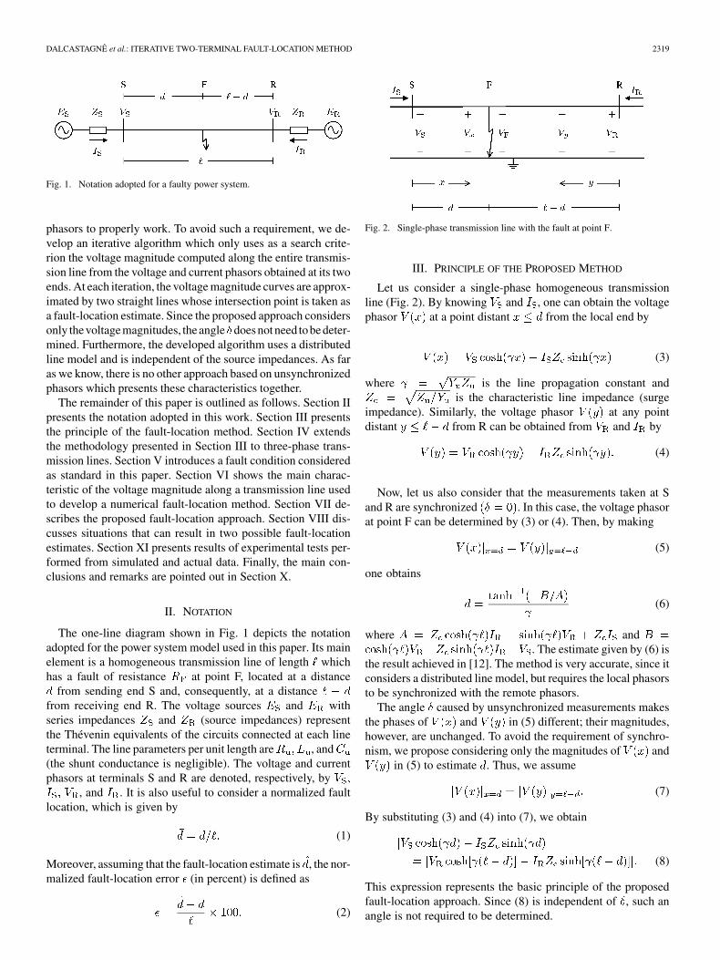
Fig. 1. Notation adopted for a faulty power system.

phasors to properly work. To avoid such a requirement, we de-velop an iterative algorithm which only uses as a search crite-rion the voltage magnitude computed along the entire transmis-sion line from the voltage and current phasors obtained at its twoends. At each iteration, the voltage magnitude curves are approx-imated by two straight lines whose intersection point is taken asa fault-location estimate. Since the proposed approach considersonly the voltagemagnitudes, the angle doesnot need to be deter-mined. Furthermore, the developed algorithm uses a distributedline model and is independent of the source impedances. As faras we know, there is no other approach based on unsynchronizedphasors which presents these characteristics together.

The remainder of this paper is outlined as follows. Section IIpresents the notation adopted in this work. Section III presentsthe principle of the fault-location method. Section IV extendsthe methodology presented in Section III to three-phase trans-mission lines. Section V introduces a fault condition consideredas standard in this paper. Section VI shows the main charac-teristic of the voltage magnitude along a transmission line usedto develop a numerical fault-location method. Section VII de-scribes the proposed fault-location approach. Section VIII dis-cusses situations that can result in two possible fault-locationestimates. Section XI presents results of experimental tests per-formed from simulated and actual data. Finally, the main con-clusions and remarks are pointed out in Section X.

II. NOTATION

The one-line diagram shown in Fig. 1 depicts the notationadopted for the power system model used in this paper. Its mainelement is a homogeneous transmission line of length whichhas a fault of resistance at point F, located at a distance

from sending end S and, consequently, at a distancefrom receiving end R. The voltage sources and withseries impedances and (source impedances) representthe Thévenin equivalents of the circuits connected at each lineterminal. The line parameters per unit length are , and(the shunt conductance is negligible). The voltage and currentphasors at terminals S and R are denoted, respectively, by

, and . It is also useful to consider a normalized faultlocation, which is given by

(1)

Moreover, assuming that the fault-location estimate is , the nor-malized fault-location error (in percent) is defined as

(2)

Fig. 2. Single-phase transmission line with the fault at point F.

III. PRINCIPLE OF THE PROPOSED METHOD

Let us consider a single-phase homogeneous transmissionline (Fig. 2). By knowing and , one can obtain the voltagephasor at a point distant from the local end by

(3)

where is the line propagation constant andis the characteristic line impedance (surge

impedance). Similarly, the voltage phasor at any pointdistant from R can be obtained from and by

(4)

Now, let us also consider that the measurements taken at Sand R are synchronized . In this case, the voltage phasorat point F can be determined by (3) or (4). Then, by making

(5)

one obtains

(6)

where and. The estimate given by (6) is

the result achieved in [12]. The method is very accurate, since itconsiders a distributed line model, but requires the local phasorsto be synchronized with the remote phasors.

The angle caused by unsynchronized measurements makesthe phases of and in (5) different; their magnitudes,however, are unchanged. To avoid the requirement of synchro-nism, we propose considering only the magnitudes of and

in (5) to estimate . Thus, we assume

(7)

By substituting (3) and (4) into (7), we obtain

(8)

This expression represents the basic principle of the proposedfault-location approach. Since (8) is independent of , such anangle is not required to be determined.


TABLE ISTANDARD POWER SYSTEM PARAMETERS

IV. EXTENSION FOR THE THREE-PHASE CASE

For the three-phase case, it is needed to apply the symmetricalcomponents or a modal transformation in order to model thethree-phase line through decoupled single-phase circuits. Then,we use in (3) and (4), the variables ,and , where denotes either the chosen mode or sequence.In a similar way as (7), is obtained from

(9)

Although any set of symmetrical or modal components canbe adopted in (9), the zero mode and zero sequence should beavoided due to the uncertainties about and . If we con-sider symmetrical components, the best choice is to use posi-tive-sequence components, which avoids a fault classificationstage, since any fault type has these sequence components. Alimitation of symmetrical components is to generate sequencecircuits which are decoupled only for transposed transmissionlines. Then, an improvement can be achieved by using Clarketransformation, which allows applying (9) to untransposed lineshaving a vertical symmetry axis [13].

The index used in (9) is dropped in this text in order tosimplify the variables notation. We assume hereafter ,which means positive sequence, because we only consider theuse of symmetrical components in this paper.

V. POWER SYSTEM UNDER STANDARD FAULT CONDITION

Hereafter, we consider as standard a phase-to-ground faultoccurring on a 500-kV power system. Its remaining parametersare shown in Table I. For simplicity, the source impedances areconsidered purely inductive due to the high-voltage level. Sucha consideration does not imply in loss of generality, since theproposed method is independent of source impedances.

All performed simulations are made using the AlternativeTransient Program (ATP) software [14]. For instance, if we saythat the power system is under the standard fault condition, thesimulation parameters are those shown in Table I. If we say that

the system is under a fault condition with , the sim-ulation parameters are equal to those presented in this section,except the fault resistance, whose value is instead of .The power system is simulated under steady-state operation, aprocedure adopted in other works [7], [12]. It avoids arising de-caying exponentials and high-frequency transients that, if nottreated correctly, lead to errors in phasor estimations (

, and , estimated by ATP). Since the phasors at S and R andthe line parameters can be considered completely correct, anyfault-location error can be attributed almost exclusively to theproposed method. Thus, the performed tests permit assessingwhether the fault-location method based only on the magnitudesof and is robust to different fault conditions. To showthat a synchronism error does not affect the proposed method,an angle is added to the remote end phasors, the samevalue used in [7].

VI. VOLTAGE ALONG A TRANSMISSION LINE

To determine in (8), it is necesary to apply a numericaltechnique. Such a process could be based on an optimizationmethod which minimizes a cost function, adopting the fault inthe middle of the line as the initial value. Two main points aboutthe use of classic optimization techniques for a fault-locationprocess based on and should be pointed out. Thefirst is that an optimization method may present high computa-cional effort. Moreover, many numerical methods employ thederivatives of functions and in this case, whichare not trivial. The second point is that as a traditional optimiza-tion method is not developed specifically for fault location, itcan suffer a convergence error in fault conditions which resultin two solutions to (7) within , depending on the ini-tial value.

The functions and present a characteristic whichpermits developing a fault-location method other than that basedon a traditional optimization method: their magnitudes calcu-lated along the whole transmission line decrease almost lin-early with the increase of distances and , respectively, whichpermit approximating satisfactorily such functions by straightlines. To show this fact, the power system under the standardfault condition is simulated. By using the phasors ,and , we use the positive sequence components in (3) and(4) to determine and , respectively, along the entiretransmission line. The magnitudes of these functions are shownin Fig. 3, in which the abscissa axis represents the distance ; thevariable is given by . Note that these curves are really verysimilar to straight lines. The functions and arevalid in Fig. 3 only until the point F ( km). How-ever, in most studied cases, the characteristics of these curvesdo not change significantly when these limits are extrapolated,which is fundamental to the correct operation of the proposedtechnique.

VII. PROPOSED METHOD

This section presents the proposed fault-location approachstep-by-step until obtaining a standard fault condition estimate.The main idea is to assume at each iteration that the fault islocated at a hypothetical point , which is located at a distance

from the local end.


Fig. 3. Magnitudes of � �� and � �� along the entire transmission line underthe standard fault condition.

A. Decoupling of Phasors

First, a modal transformation is applied or the symmetricalcomponents for phasors measured at the line ends are computed.Here, we adopt the symmetrical components and use the posi-tive sequence in (9). Since the studied line is transposed, such atransformation results in decoupled sequence components.

B. Initial Value

As Fig. 3 shows, the functions and can be sat-isfactorily approximated by straight lines. In this case, isapproximated by a first-order equation defined by

(10)

In the same way, the function is given by

(11)

Note that is a function of , but is expressed as afunction of , since . Such a procedure makes itpossible to equate and and define an intersection pointbetween these lines in terms of variable .

Let us then consider Fig. 4; the angular coefficients andare related to the slopes of at and at ,respectively. Thus, they represent the derivatives of at

and at . To avoid the necessity of performinga derivative operation and considering that the exact knowledgeof these coefficients is irrelevant, and are approximatedby evaluating (3) and (4) by finite differences with close valuesof . In this paper, they are defined by

(12)

and

(13)

Fig. 4. Straight lines � and � which define the initial estimate � ��.

The linear coefficients and define the values of andat , respectively. Through Fig. 4, we conclude that

(14)

and

(15)

The intersection between and at each iteration definesthe location of the hypothetic fault point . By equating(10) with (11) and considering , we define that theinitial fault-location estimate is given by

(16)

By applying (12)–(16), the proposed algorithm defines an ini-tial estimate for the standard fault km.

C. Iteration

The functions and at an iteration are slightly differentfrom those used to define . To speed up convergence, theinformation which defines the coefficients of and are ex-tracted from point . Let us consider Fig. 5, whichpresents and at the first iteration. It should be noted thatthe necessity of applying an independent variable transforma-tion to displace the axis origin to point . Forthis, the distance in (10) and (11) is replaced by ,resulting in

(17)

and

(18)

The angular coefficients and represent, respectively, theslopes of and at . As adopted earlier,these coefficients are approximated through the values ofand by finite differences. For such, we use

(19)


Fig. 5. Straight lines � and � at iteration � � �.

and

(20)

The linear coefficients and define the values of andat , respectively. Thus

(21)

and

(22)

By equating (17) with (18), considering , and makingthe appropriate mathematical manipulations, we define that thefault-location estimate at each iteration is given by

(23)

By using (19)–(23), the algorithm defineskm. In a single iteration, the fault-location estimate is almostequal to the actual standard fault location km.

D. Iteration

Since the proposed approach is iterative, it is necessary toadopt a stopping criterion. We declare convergence at iteration

, when

(24)

where . As the process is stopped at this iteration ,the fault-location estimate is

(25)

If is sufficiently small, the part of fault-location error due tothe stopping criterion is negligible. The performed evaluationtests lead us to claim that is reasonable for obtaininga good method performance. For the standard fault condition,the algorithm converges in two iterations given an estimate

km, whose error is %.This negligible error can be attributed to the following causes.

Fig. 6. Magnitudes of � �� and � �� along the entire transmission line for aphase-to-ground fault condition with � � �� and � � � km � �� .

1) Finite precision of variable numerical representations andarithmetic operations considered during the successive ap-proximation process.

2) Small errors in phasor estimates.3) Necessity of adopting a stopping criterion.

VIII. MULTIPLE SOLUTION CASES

In some situations, and/or are not so well be-haved as those shown in Fig. 3. In these cases, it may occur asa risk situation for a fault-location method based only on themagnitudes of and : the curves and/orevaluated for may present two intersecting points,which means that (7) has two possible solutions and lo-cated within the transmission-line length. In this paper, thesecases are classified as Type 1 and Type 2 faults.

A. Type 1

In this case, only one magnitude curve oris heavily curved along the entire transmission line, resultingin solutions and far from each other. Phase-to-ground,phase-to-phase, and phase-to-phase-to-ground faults may resultin Type 1 faults.

A Type 1 fault occurs for a phase-to-ground fault conditionwith located at the local end. Fig. 6 shows the curves

and from which we verify the intersection pointskm and km. Note that

is the correct solution, although its value is slightly larger thanzero (the value of used in ATP). This difference can be at-tributed to causes 1) and 2) pointed out in the previous section.Table II presents the proposed technique estimates. The methodconverges to the correct solution , resulting in a negligiblefault-location error %. In all studied Type 1faults, the proposed method converges correctly. Type 1 faultsare rare and normally occur for fault conditions close to trans-mission-line ends ( and ).

The algorithm converges to the right solution because the ini-tial value is located in a region in which and


TABLE IIFAULT-LOCATION ESTIMATES FOR A PHASE-TO-GROUND

FAULT CONDITION WITH � � �� AND � � ��

are very close to straight lines. Such a fact is not true beyondkm, when the curve presents a minimum point.

Thus, only the part of , which has an almost linear char-acteristic, is used by the algorithm. If the initial estimate wouldbe larger than 50 km, the numerical process could converge tothe wrong solution. Fortunately, this fact is never verified in theType 1 faults studied in this paper.

B. Type 2

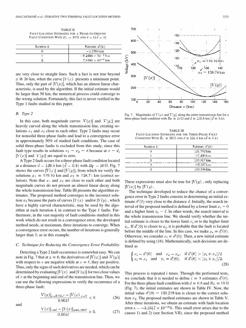
In this case, both magnitude curves and areheavily curved along the whole transmission line, creating so-lutions and close to each other. Type 2 faults may occurfor nonsolid three-phase faults and lead to a convergence errorin approximately 50% of studied fault conditions. The case ofsolid three-phase faults is excluded from this study, since thisfault type results in solutions because at

and are equal to zero.A Type 2 fault occurs for a three-phase fault condition located

at a distance km with . Fig. 7shows the curves and , from which we verify thesolutions km and km (correct so-lution). Note that and are close to each other and bothmagnitude curves do not present an almost linear decay alongthe whole transmission line. Table III presents the algorithm es-timates. The proposed method converges to the incorrect solu-tion because the parts of curves and/or , whichhave a highly curved characteristic, may be used by the algo-rithm at each iteration in contrast to the Type 1 faults. Fur-thermore, in the vast majority of fault conditions studied in thiswork which do not result in a convergence error, the developedmethod needs, at maximum, three iterations to converge. Whena convergence error occurs, the number of iterations is generallylarger than 3, as in this example.

C. Technique for Reducing the Convergence Error Probability

Detecting a Type 2 fault occurrence is somewhat easy. We cannote in Fig. 7 that at , the derivatives of andwith respect to are negative while at , they are positive.Thus, only the signs of such derivatives are needed, which can bedetermined by evaluating and for two close valuesof at the beginning and end of the transmission line. Then, wecan use the following expressions to verify the occurrence of athree-phase fault:

(26)

and

(27)

Fig. 7. Magnitudes of � �� and � �� along the entire transmission line for athree-phase fault condition with � � �� and � � �� km � �� .

TABLE IIIFAULT-LOCATION ESTIMATES FOR THE THREE-PHASE FAULT

CONDITION WITH � � �� AND � � �� km � ��

These expressions must also be true for , only replacingby .

The technique developed to reduce the chance of a conver-gence error in Type 2 faults consists in determining an initial es-timate very close to the distance . Initially, the search in-terval of the proposed method is defined by a lower limitand a higher limit . In other words, the search interval isthe whole transmission line. We should verify whether the ini-tial estimate is closer to the lower limit or to the higher limit

. If is closer to , it is probable that the fault is locatedbefore the middle of the line. In this case, we make .Otherwise, we consider . Then, a new initial estimateis defined by using (16). Mathematically, such decisions are de-fined as

and ifand if

(28)

This process is repeated times. Through the performed tests,we conclude that it is needed to define estimates .For the three-phase fault condition with and(Fig. 7), the initial estimates are shown in Table IV. Now, theinitial value km is closer to the correct solu-tion . The proposed method estimates are shown in Table V.After three iterations, we obtain an estimate with fault-locationerror %. This small error arises due to thecauses 1) and 2) (see Section VII), since the proposed method


TABLE IVINITIAL VALUES FOR THE THREE-PHASE FAULT CONDITION WITH � � ��

AND � � �� km � �� CONSIDERING � �

TABLE VFAULT-LOCATION ESTIMATES FOR THE THREE-PHASE FAULT CONDITION WITH

� � �� AND � � �� km � �� , CONSIDERING AS INITIAL VALUE

� �� km

TABLE VIRESULTS FOR PHASE-TO-GROUND FAULT CONDITIONS WITH � � � � km

� �� AND DIFFERENT FAULT RESISTANCES

converges correctly to (Fig. 7), except for a small differencecaused by the stopping criterion.

IX. EXPERIMENTAL RESULTS

A. Conditions Adopted in the Simulations

First, the power system defined in Section V is simulated withATP under steady-state operation so that the phasors can be con-sidered accurate. Since the line parameters are known, this is aperfect condition to apply the proposed method. Thus, if a con-vergence error is not observed, the fault-location errors shouldalso be null, except for small errors caused by factors 1) to 3)(Section VII). Again, we adopt and .

B. Variation of Fault Resistance

Here, we vary the fault resistance from zero (solid fault) to(high fault resistance), with steps. Since the model

used in this work is independent of , such a parameter shouldnot influence the technique performance. Table VI shows theresults. None of the studied conditions results in two solutionsto (7) within . The number of iterations is two or threeand the fault-location errors are negligible.

C. Variation of Distance

Here, we consider phase-to-ground faults located from ter-minal S to terminal R by varying in stepsof 0.2. Table VII shows the results. Only the fault condition with

TABLE VIIRESULTS FOR PHASE-TO-GROUND FAULT CONDITIONS WITH � � �� AND

DIFFERENT FAULT LOCATIONS

TABLE VIIIRESULTS FOR PHASE-TO-GROUND FAULT CONDITIONS WITH � � ��

� � � � km � �� AND DIFFERENT LINE LOAD CONDITIONS

, Type 1 fault studied in Section VIII, results in two so-lutions to (7) within . In all cases, the algorithmneeds only two iterations to converge and presents a negligiblefault-location error, of the order of for the worst cases.Thus, we can conclude that the performance of the proposedtechnique is not affected by the fault location.

D. Variation of Line Load

To simulate line load variations, we change the magnitude andphase of the , procedure similar to that adopted in [15] and[16]. In this paper, five load conditions are studied as follows.

1) Normal power flow, for which the magnitude of is 500kV and its phase is (standard fault).

2) The magnitude of is changed to 450 kV.3) The magnitude of is changed to 550 kV.4) The phase of is changed to .5) The phase of is changed to .Table VIII presents the results. Again, none of the considered

fault conditions result in two solutions to (7) within .Moreover, the fault-location errors are negligible, of the orderof in the worst case [condition (e)]. Thus, we can considerthat the proposed method is not significantly affected by the lineload condition.

E. Variation of Fault Type

To verify the robustness of the proposed approach to differentfault conditions, it is insufficient to consider faults located onlyat a single point, such as km. Then, we vary the lo-cation of each fault type from the local until the remote end, insteps of 0.2 . The case of phase-to-ground fault conditionshas already been studied in Section IX-C.

Table IX shows the results for the phase-to-phase fault con-ditions located along the transmission line. In all cases, the al-gorithm presents a negligible fault-location error, converging in


TABLE IXRESULTS FOR PHASE-TO-PHASE FAULT CONDITIONS WITH � � ��

LOCATED ALONG THE TRANSMISSION LINE

TABLE XRESULTS FOR PHASE-TO-PHASE-TO-GROUND FAULT CONDITIONS WITH

� � �� LOCATED ALONG THE TRANSMISSION LINE

TABLE XIRESULTS FOR THREE-PHASE FAULT CONDITIONS WITH � � �� LOCATED

ALONG THE TRANSMISSION LINE, WITHOUT USING THE TECHNIQUE OF

DEFINING � INITIAL VALUES � ��. THE HIGHLIGHTED LINES REPRESENT THE

CASES IN WHICH A CONVERGENCE ERROR OCCURS

only one iteration. Again, the fault condition located at the localend results in two solutions to (7) within .

Table X shows the results for the phase-to-phase-to-groundfault conditions. Again, the fault-location error is negligible.The fault conditions with that are equal to 0.6 and 1.0 convergein a single iteration; the remaining cases need two iterations. Inthese tests, the fault conditions located at local and re-mote terminal generate two solutions to (7) within

(Type 1 faults).Table XI shows the results for three-phase fault conditions.

Only the fault condition with does not present two so-lutions to (7) within ; the remaining ones are Type2 faults. The algorithm leads to a convergence error in half ofthe studied cases. To solve the convergence problem in thesesituations, we apply the technique of defining initial valuesdeveloped in Section VIII-C. Table XII shows the results afterapplying such a technique with . Now, the algorithm con-verges to the correct solution in all situations.

F. Experimental Tests With Other Power Systems

Until here, we presented the results of experiments consid-ering only the power system defined in Section V. To verify themethod’s efficiency beyond this particular power system, tests

TABLE XIIRESULTS FOR THREE-PHASE FAULT CONDITIONS WITH � � �� LOCATED

ALONG THE TRANSMISSION LINE, BY USING THE TECHNIQUE OF DEFINING �

INITIAL VALUES �� DISCUSSED IN SECTION VIII-C

TABLE XIIIFAULT-LOCATION ESTIMATES OF THE PROPOSED METHOD CONSIDERING A

PHASE-TO-GROUND FAULT CONDITIONS WITH � � �� LOCATED ALONG

THE TRANSMISSION LINE AND DIFFERENT VALUES FOR �

similar to those presented before are also performed in two otherpower systems with the configuration shown in Fig. 1. Since theresults are very similar to the obtained with the standard powersystem, these results are not presented in this paper.

G. Sensitivity for a Synchronism Error

To show the effect of a synchronism error in two-terminalfault-location methods, we compare the proposed method withthe well-known approach introduced in [12]. The only differ-ence is that we consider here the use of positive sequence insteadof aerial mode 1 (from Clarke transformation) used in [12]. Inthese tests, we consider again phase-to-ground fault conditionswith resistance .

Table XIII presents the proposed method estimates forand . Naturally, these estimates are equal, independentof . Furthermore, they are equal to those obtained for a evenhigher ( , Table VII).

Table XIV shows the estimates obtained by the approach [12].For , they present small imaginary parts. Fig. 8, which cor-responds to the standard fault condition, illustrates the origin ofthe small imaginary parts of the estimates given in Table XIVfor . The method discussed in [12] is based on (5). Thus,both magnitude and phase of and should be equalat . However, numerical errors due to causes 1) and2) (Section VII) lead to the intersections between magnitudecurves [Fig. 8(a)] and phase curves [Fig. 8(b)] to be slightly dif-ferent (64.3990 km and 64.3981 km, respectively). In this way,the estimates using [12] present negligible imaginary parts. For

, the estimate imaginary parts are comparable to realparts (see Table XIV). Fig. 9 shows the phases of andfor the standard fault condition with [the magnitudecurve is shown in Fig. 8(a)]. In this case, the intersection pointsbetween magnitude and phase curves of and occur


Fig. 8. Functions � �� and � �� for the standard fault condition and angle� � �. (a) Magnitude curves. (b) Phase curves.

in two different values of km [see Fig. 8(a)]and km [see Fig. 9], respectively. Thus, it is im-possible to define a real which satisfies the condition (5) interms of magnitude and phase. This fact is the origin of the highimaginary parts of estimates for unsynchronized phasors whenusing [12].

Table XV presents the fault-location error of estimates shownin Tables XIII and Tables XIV. The fault-location error (in per-cent) of the method given in [12] is evaluated considering onlythe real part of the fault-location estimate. Thus

(29)

In an ideal situation (in which phasors and line parameters areexempt from errors), the techniques present negligible fault-lo-cation errors if the phasors of two terminals are synchronized

. For nonsynchronized measures, the fault-location errorof the method from [12] is high while the proposed approachpresents the same fault location error for any .

Fig. 9. Phases of � �� and � �� for the standard fault condition and angle� � �� .

TABLE XIVFAULT-LOCATION ESTIMATES OBTAINED BY THE APPROACH [12], CONSIDERING

PHASE-TO-GROUND FAULT CONDITIONS WITH � � �� LOCATED ALONG

THE TRANSMISSION LINE AND DIFFERENT VALUES FOR �

H. Sensitivity to Instrument Transformer Errors

Here, we study the effect of instrument transformer errors onthe accuracy of the proposed fault-location method. To simulateinstrument transformer errors, we apply shifts in magnitudesand phases of phasors measured at both ends of the transmissionline presented in Section V, which presents a phase-to-groundfault condition with resistance located atkm (standard fault condition). Then, we apply the method devel-oped in [12] (Method I) and the proposed technique (Method II)and verify the fault-location error of both approaches in ten dif-ferent cases.

First, we consider the influence of transformer instrumentsin phasor magnitude errors. Potential transformers normallypresent a class of accuracy of 0.3%, 0.6%, or 1.2%, whileCTs for protection are normally specified with 2.5% or 10%of error. Table XVI shows the conditions considered in thisstudy, which consist in different combinations of the worstpossible transformer errors: 1.2% for potential transformersand 10% for CTs. Table XVII shows the results of Cases 1to 4. Cases 1 and 2 represents the worst possible conditions,since the phasors of a terminal increase while the phasors ofthe other terminal decrease. We verify that both techniques areaffected in such situations; however, the approach presented in[12] exhibits better performance. In Cases 3 and 4, one phasor


TABLE XVFAULT-LOCATION ERROR OF ESTIMATES GIVEN IN TABLES XIII AND XIV:

REFERENCE [12] METHOD (I). PROPOSED METHOD (II)

TABLE XVIERRORS IN PHASOR MAGNITUDES

TABLE XVIIFAULT-LOCATION ERRORS OF CASES 1 TO 4 CONSIDERING THE METHOD

PROPOSED IN [12] (METHOD I) AND THE METHOD PROPOSED IN THIS WORK

(METHOD II)

of each terminal decreased while the other increased. Then,the variation is not completely positive or negative in eachterminal. Consequently, both methods are not so much affectedin these situations. However, we can observe in Table XVIIthat the proposed approach is more accurate than the approachpresented in [12] for theses cases. In Cases 5 and 6, the phasormagnitudes of both terminals are shifted by the same factor.Thus, such variations do not affect the fault-location errorof the considered fault-location methods. In these cases, thefault-location errors are of the order of or , whichmakes it unnecessary to present the results.

Now, we consider the influence of the phase error of instru-ment transformers on the fault-location accuracy. As such, weadopt the strategy of varying the phasor phases by (the threephases), as shown in Table XVIII. Table XIX shows the obtainedresults. In Cases 7 and 8, the phasors of each terminal are shiftedby the same amount . Thus, the phase between the voltageand current phasors of each terminal does not change. This situ-ation is equivalent to add a synchronism error betweenthe phasors of terminals S and R. As shown in Section IX-G,the proposed method is immune to such a parameter while theapproach proposed in [12] is very affected by such a source oferror. We verify that the errors of the proposed method in thesecases are negligible, and equal to those obtained in Section VII,considering an even higher synchronism error . Onthe other hand, the errors of the approach presented in [12] for

TABLE XVIIIERRORS IN PHASOR PHASES

TABLE XIXFAULT-LOCATION ERRORS OF CASES 7 TO 10 CONSIDERING THE METHOD

PROPOSED IN [12] (METHOD I) AND THE PROPOSED METHOD (METHOD II)

TABLE XXPARAMETERS OF THE STUDIED ACTUAL FAULT CONDITIONS (FCS)

these cases are high. Now, consider the Cases 9 and 10. In thesesituations, the phases between the voltage and current phasorsof each terminal are changed. In this way, these cases includeother error sources than synchronism error, which results in bothmethods obtaining inaccurate estimates. Table XIX shows thatthe approach presented in [12] is slightly better than the pro-posed method for these cases.

I. Analysis With Actual Data

This section presents experimental tests performed fromfour actual fault conditions (phase-to-ground faults) occurringin two transposed and homogeneous transmission lines (seeTable XX). The sampling frequency of signals is 1920 Hz(32 samples/cycle) and the measurements are synchronized

.Since the data are real, in this study, we have errors in pha-

sors and line parameters. Moreover, we do not know informa-tion about the data measuring and phasor estimation stages. Forexample, the class of accuracy of current and potential trans-formers is unknown. Another point which can impair the fault-location method evaluation is that the real fault location is mea-sured with a precision of 1 km, as Table XX shows. Such a preci-sion represents, for instance, the smaller line considered in thissection ( km, fault condition 4) that the real mea-surement may have a maximal error of 0.6% of the length .As the fault-location error represents a percentage of the trans-mission-line length, this precision error is naturally added to thefault-location error.

These actual fault conditions (FCs) are located by applyingthe approach from [12] (Method I) and the proposed approach(Method II). Such a comparison is valid, since both techniquespresent similar performance for synchronized phasors. Since the


TABLE XXIRESULTS OF THE ACTUAL FAULT CONDITIONS BY APPLYING THE APPROACH

GIVEN IN [12] (METHOD I) AND THE PROPOSED APPROACH (METHOD II)

method given in [12] is considered to be one of the best pro-posed in the literature, used even in commercial fault locators,the comparison of its performance with the proposed methodallows validating the developed technique, even if the fault-lo-cation error in some fault conditions is somewhat inaccurate dueto errors in phasors and transmission-line parameters.

Table XXI shows the obtained results. The proposed methodconverges in two iterations for these four fault conditions. Theestimates from both methods present nonnegligible fault-loca-tion errors. It can be attributed to errors in phasors, in transmis-sion-line parameters, and to the precision of the actual fault-lo-cation measure. Comparing the two techniques, the proposedmethod is better in two cases (fault conditions 2 and 3); themethod given in [12] is better in one case (fault condition 1);in one case, the techniques present similar performance (faultcondition 4). Such results show that the performance of the con-sidered techniques are similar for synchronized phasors. If thephasors are unsynchronized, the performance of the method pro-posed in [12] tends to decline, while the proposed technique isnot affected by a synchronization error.

Although the proposed method does not present a negligiblefault-location error in the four studied actual fault conditions,the algorithm converges correctly to the intersection point be-tween the curves and . Fig. 10 shows the magni-tude and phase curves of and for the fault condi-tion 2. Note that the intersection points between the magnitudecurves ( km) and phase curves ( km)are different. However, the fault-location estimate of the pro-posed method is 52.19 km. Thus, the fault-location error arisesdue to the doubtful quality of phasors and line parameters usedin the fault-location processes and not due to the developed nu-merical process.

X. CONCLUDING REMARKS

This paper has presented a novel two-terminal impedance-based fault-location algorithm. The proposed approach uses thesame line model adopted in [12], with the advantage of not re-quiring synchronism between the phasors taken at local and re-mote transmission-line ends. The fact of being based only onthe magnitude of voltages across the entire transmission line cangive rise to two possible solutions to the fault-location estimatefor nonsolid three-phase fault conditions, which may lead theproposed approach to converge to the incorrect solution in suchsituations. To solve this problem, an auxiliary technique is de-veloped, which decreases substantially the possibility of a con-vergence error. The results obtained from tests with fault condi-tions simulated with ATP showed that the proposed approach

Fig. 10. Functions � �� and � �� of fault condition 2. (a) Magnitude curves.(b) Phase curves.

has a negligible fault-location error if phasors and transmis-sion-line parameters are accurate. For actual fault conditions,the fault-location error magnitude depends on the accuracy ofphasors and transmission-line parameters. However, the algo-rithm tends to be equivalent to the method given in [12] foractual synchronized data. In the case of unsynchronized data,the proposed approach performance is much better than the ap-proach given in [12] which presents high sensitivity to synchro-nism errors.

ACKNOWLEDGMENT

The authors would like to thank the Associate Editor and theanonymous reviewers for their valuable and constructive com-ments and suggestions, from which the revision of this paperhas benefited significantly.


REFERENCES

[1] T. W. Stringfield, D. J. Marihart, and R. F. Stevens, “Fault locationmethods for overhead lines,” AIEE Trans. Power App. Syst., vol. 76, pt.3, pp. 518–530, Aug. 1957.

[2] E. Born and J. Jaeger, “Device locates point of fault on transmissionlines,” Elect. World, vol. 168, pp. 133–134, Jul. 1967.

[3] T. Takagi, Y. Yamakoshi, J. Baba, K. Uemura, and T. Sakaguchi, “Anew algorithm of an accurate fault location for EHV/UHV transmissionlines: Part I - Fourier transformation method,” IEEE Trans. Power App.Syst., vol. PAS-100, no. 3, pp. 1316–1322, Mar. 1981.

[4] T. Takagi, Y. Yamakoshi, M. Yamaura, R. Kondow, and T. Mat-sushima, “Development of a new type fault locator using theone-terminal voltage and current data,” IEEE Trans. Power App. Syst.,vol. PAS-101, no. 8, pp. 2892–2898, Aug. 1982.

[5] L. Eriksson, M. M. Saha, and G. D. Rockefeller, “An accurate faultlocator with compensation for apparent reactance in the fault resistanceresulting from remote-end infeed,” IEEE Trans. Power App. Syst., vol.104, no. 2, pp. 424–436, Feb. 1985.

[6] “IEEE guide for determining fault location on ac transmission anddistribution lines,” Jun. 2005.

[7] D. Novosel, D. G. Hart, E. Udren, and J. Garitty, “Unsynchronizedtwo-terminal fault location estimation,” IEEE Trans. Power Del., vol.11, no. 1, pp. 130–138, Jan. 1996.

[8] A. A. Girgis, D. G. Hart, and W. L. Peterson, “A new fault locationtechnique for two- and three-terminal lines,” IEEE Trans. Power Del.,vol. 7, no. 1, pp. 98–107, Jan. 1992.

[9] I. Zamora, J. F. Miambres, A. J. Mazn, R. Alvarez-Isasi, and J. Lazaro,“Fault location on two-terminal transmission lines based on voltages,”Proc. Inst. Elect. Eng., Gen., Transm. Distrib., vol. 143, no. 1, pp. 1–6,Jan. 1996.

[10] P. Balcerek and J. Izykowski, “Improved unsynchronized two-end al-gorithm for locating faults in power transmission lines,” presented atthe IEEE Bologna PowerTech Conf., Bologna, Italy, Jun. 2003.

[11] A. L. Dalcastagnê, S. Noceti Filho, H. H. Zürn, and R. Seara, “A two-terminal fault location approach based on unsynchronized phasors,”in Proc. Int. Conf. Power System Technology, Chongqing, China, Oct.2006, pp. 1–7.

[12] A. T. Johns and S. Jamali, “Accurate fault location technique for powertransmission lines,” Proc. Inst. Elect. Eng., vol. 137, no. 6, pp. 395–402,Nov. 1990.

[13] M. C. Tavares, J. Pissolato, and C. M. Portela, “New mode-domainmultiphase transmission line model—Clarke transformation evalua-tion,” in Proc. Int. Conf. Power System Technology , Beijing, China,Aug. 1998, vol. 2, pp. 860–864.

[14] “Alternative Transient Program, User Manual and Rule Guide,” 1989,European EMTP-ATP User’s Guide.

[15] J.-A. Jiang, Y.-H. Lin, J.-Z. Yang, T.-M. Too, and C.-W. Liu, “Anadaptive PMU based fault detection/location technique for transmis-sion lines—Part II: Implementation and performance evaluation,” IEEETrans. Power Del., vol. 15, no. 4, pp. 1136–1146, Oct. 2000.

[16] D. J. Lawrence, L. Z. Cabeza, and L. T. Hochberg, “Development ofan advanced transmission line fault location system part II: Algorithmdevelopment and simulation,” IEEE Trans. Power Del., vol. 7, no. 4,pp. 1972–1983, Oct. 1992.

André Luís Dalcastagnê was born in Florianópolis,Brazil. He received the B.E., M.Sc., and Ph.D. de-grees from the Federal University of Santa Catarina,Florianópolis, in 2000, 2002, and 2007, respectively,all in electrical engineering.

He joined the Department of Electronics, FederalTechnological Education Center of Santa Catarina in2006. His research interests include analog filtering,power quality, and transmission-line fault location.

Sidnei Noceti Filho was born in Florianópolis,Brazil. He received the B.E. and M.Sc. degrees inelectrical engineering from the Federal Universityof Santa Catarina, Florianópolis, Brazil, in 1975 and1980, respectively, and the Ph.D. degree in electricalengineering from the Federal University of Rio deJaneiro, Rio de Janeiro, Brazil, in 1985.

In 1976, he joined the Department of Electrical En-gineering at the Federal University of Santa Catarina,where he has been engaged in education and researchin signal processing and circuit analysis and design.

He has been Professor of electrical engineering at the Federal University ofSanta Catarina since 1993.

Hans Helmut Zürn (M’75–SM’06) received the en-genheiro mecânico-eletricista degree from the Fed-eral University of Rio Grande do Sul, Porto Alegre,Brazil, in 1966, the M.Sc. degree from the Universityof Houston, Houston, TX, in 1969, and the Ph.D. de-gree from the University of Waterloo, Waterloo, ON,Canada, in 1976.

Currently, he is with the Department of ElectricalEngineering, Faculty of the Federal University ofSanta Catarina, Florianópolis, Brazil, where hehas been since 1967. His current research interests

include power systems operation and distributed-generation modeling.

Rui Seara (M’93–SM’04) was born in Florianópolis,Brazil. He received the B.E. and M.Sc. degrees inelectrical engineering from the Federal University ofSanta Catarina, Florianópolis, in 1975 and 1980, re-spectively, and the Ph.D. degree in electrical engi-neering from the Paris-Sud University, Paris, France,in 1984.

He joined the Department of Electrical Engi-neering at the Federal University of Santa Catarinain 1976, where he is currently a Professor of elec-trical engineering and Director of LINSE—Circuits

and Signal Processing Laboratory. His research interests include digital andanalog filtering, adaptive signal-processing algorithms, image and speechprocessing, and digital communications.

2318 ieee transactions on power delivery, vol. 23, …

Documents