application of transient based methods for improving the
TRANSCRIPT
Application of Transient Based Methods for
Improving the Selectivity and Speed of Protection
Systems Used in Active Distribution Networks
By
Amila Karasin Pathirannahalage
A thesis submitted to the Faculty of Graduate Studies of
The University of Manitoba
in partial fulfilment of the requirements for the degree of
DOCTOR OF PHILOSOPHY
Department of Electrical and Computer Engineering
University of Manitoba
Winnipeg
Copyright ©2019 by Amila Karasin Pathirannahalage

ii
Dedication
To my Father, Mother, and Wife.

iii
Abstract
The interconnection of distributed energy resources (DER) alters the radial structure of
distribution systems and the character of fault currents resulting in delayed operation, reduced
sensitivity, or loss of coordination of the traditional protection algorithms that rely on the
fundamental frequency current and voltage phasors. Alternative protection techniques that are
more immune to problems created by DER can be developed using fault generated transients in
the currents and voltages, but they suffer from the lack of security against the transients from
normal events, limited bandwidth of instrument transformers, need for hardware with high-
frequency sampling and signal processing power. This thesis examine methods to overcome the
above concerns with respect to a transient based protection algorithm that relies on a comparison
of the polarity of current transients observed at the boundary of a protected zone.
In order to accurately measure current transient polarities without additional digital signal
processing resources, a new sensor consisting of a ferrite core coil and analog electronics is
proposed. A detailed model of the sensor including frequency-dependent hysteresis characteristics
of the ferrite core was developed for simulation studies. The model was implemented in PSCAD
electromagnetic transient simulation software and validated against a sensor prototype.
The security of protection against the non-fault related transients is improved through a
hybrid protection structure that combines the transient based protection algorithm with traditional
overcurrent or distance protection. The application of the proposed hybrid protection scheme in
conjunction with overcurrent and distance elements was implemented and the benefits of faster
protection achieved with the proposed method was demonstrated through case studies. The
proposed protection scheme was then applied to a large distribution network to verify its reliability.
The proposed hybrid protection scheme can be easily incorporated into existing
commercial relays using the transient polarity sensor developed in this thesis, eliminating the need
for protection relays with high frequency sampling. The performance of such implementation was
tested using hardware-in-the-loop simulations with a real-time digital simulator.

iv

v
Table of Contents
Chapter 1 1
1.1 Background ............................................................................................ 1
1.2 Motivation .............................................................................................. 5
1.3 Problem definition.................................................................................. 6
1.4 Objectives of the research ...................................................................... 8
1.5 Thesis overview ...................................................................................... 9
Chapter 2 11
2.1 Introduction .......................................................................................... 11
2.2 Methods of fault isolation in distribution networks ........................... 12
2.2.1 Fuses .......................................................................................... 12
2.2.2 Sectionalizers............................................................................. 14
2.2.3 Reclosers .................................................................................... 15
2.2.4 Overcurrent relay ...................................................................... 16
2.2.5 Directional overcurrent relays .................................................. 17
2.3 Operation of reclosers and sectionalizers ........................................... 19
2.4 Coordination of various protection devices ......................................... 22
2.4.1 Fuse-fuse coordination .............................................................. 22
2.4.2 Recloser-fuse coordination ........................................................ 23
2.4.3 Recloser-relay coordination ....................................................... 25
2.5 Protection of a ring distribution grid structure .................................. 25
2.6 Protection issues of active distribution networks ............................... 28
2.6.1 Blinding of protection ................................................................ 30
2.6.2 False tripping ............................................................................ 32
2.6.3 Recloser issues ........................................................................... 33
2.6.4 Unnecessary islanding .............................................................. 35
2.6.5 Synchronization issues .............................................................. 36

vi
2.6.6 Communication issues .............................................................. 37
2.6.7 Stability issues .......................................................................... 37
2.7 Transient stability of synchronous generators ................................... 38
2.8 Protection methods used in active distribution networks .................. 42
2.8.1 Differential protection methods ................................................ 42
2.8.2 Impedance based protection methods ...................................... 43
2.8.3 Adaptive protection schemes .................................................... 43
2.9 Protection algorithms based on transient signals .............................. 44
2.9.1 Protection based on incremental Signals ................................. 45
2.9.2 Protection based on traveling waves ........................................ 47
2.9.3 Protection using signal-processing methods ............................ 48
Chapter 3 51
3.1 Introduction .......................................................................................... 51
3.2 Detection of polarity of transients ....................................................... 51
3.2.1 Signal processing methods ........................................................ 52
Mathematical Morphology ........................................................................ 53
3.2.2 Measurement of transients ....................................................... 54
3.3 Design and operation of the current transient sensor ....................... 55
3.3.1 Selection of ferrite core coil ....................................................... 59
3.3.2 Comparison with other core types ............................................ 60
3.4 Mathematical model of ferrite core sensor.......................................... 65
3.4.1 Modeling of hysteresis of the ferrite core ................................. 67
3.4.2 Inclusion of dynamic behavior .................................................. 69
3.4.3 EMT simulation model of the ferrite core coil.......................... 70
3.5 Validation of the ferrite core coil model .............................................. 71
3.5.2 Output voltages in response to current transients .................. 75
3.6 Comparison of the proposed transient detection method (ferrite cored coil)
with digital signal processing approaches .................................................. 77

vii
3.6.1 Wavelet Transform .................................................................... 77
3.6.2 Mathematical Morphology ........................................................ 80
3.7 Summary .............................................................................................. 84
Chapter 4 85
4.1 Introduction .......................................................................................... 86
4.2 Faulty section identification using current transients....................... 87
4.3 Hybrid protection method .................................................................... 88
4.4 Faulted zone identification .................................................................. 94
4.5 Case Study I –Demonstration of Basic Principle................................ 97
4.5.1 Transient polarity extraction .................................................. 100
4.5.2 Simulation results and discussion .......................................... 103
4.5.3 Sensitivity of the transient detection ..................................... 111
4.5.4 Effect of converters for transient polarity detection .............. 115
4.6 Case Study II - Solving potential DER stability problems with the hybrid
protection approach.................................................................................... 117
4.6.1 Identified stability issues ........................................................ 119
4.6.2 Protection using the hybrid protection scheme ...................... 122
4.7 Case Study III - Application to 34-bus distribution network ........... 126
4.8 Security of the protection scheme ..................................................... 135
4.8.2 Connection of a generator ....................................................... 138
4.8.3 Disconnection of a generator................................................... 139
4.8.4 Three-phase fault .................................................................... 141
4.8.5 Line-Ground Fault .................................................................. 142
Chapter 5 148
5.1 Introduction ........................................................................................ 148
5.2 Implementation of protection concept ............................................... 149
5.2.1 Hardware implementation of the sensor ................................ 151

viii
5.2.2 Integration of the external protective relay ........................... 152
5.2.3 Integration of hybrid protection scheme with the power network
simulated in RTDS simulator ............................................................ 154
5.3 Results & discussion .......................................................................... 157
5.3.1 Internal Fault .......................................................................... 157
5.3.2 External fault .......................................................................... 162
5.4 Summary ............................................................................................ 164
Chapter 6 166
6.1 Conclusions ........................................................................................... 166
6.2 Contributions ..................................................................................... 168
6.3 Future work........................................................................................ 170
Appendix A 172
Appendix B 174
Appendix C 178
Bibliography 186
ix
List of Figures
Figure 2-1 Operating characteristics of a fuse ........................................................................... 14
Figure 2-2 A typical North American distribution feeder .......................................................... 21
Figure 2-3 Fuse-fuse coordination ............................................................................................ 23
Figure 2-4 Fuse-relay coordination ........................................................................................... 24
Figure 2-5 Ring distribution network structure with normally open switch ............................... 26
Figure 2-6 Ring distribution network structure ......................................................................... 27
Figure 2-7 Ring network as a radial network with two sources ................................................. 28
Figure 2-8 Illustration the effects of blinding of protection for downstream faults..................... 31
Figure 2-9 Equivalent circuit of Fig 2-8 .................................................................................... 31
Figure 2-10 Thevenin equivalent of Fig. 2-9 ............................................................................. 31
Figure 2-11 False tripping ........................................................................................................ 33
Figure 2-12 Recloser operation affected by DER ...................................................................... 34
Figure 3-1 Current transient polarity detection sensor ............................................................... 56
Figure 3-2 Response of the sensor for a fault current (a) input primary current, (b) ferrite core coil
output voltage, (c) coil voltage after high pass filter, and (d) Tn output of latching circuit ........ 59
Figure 3-3 Experimental setup designed to compare different core types .................................. 61
Figure 3-4 Output voltage response of different core types while the core is unsaturated .......... 62
Figure 3-5 Response to transient currents when the ferrite core is saturated .............................. 63
Figure 3-6 Arrangement of the transient detecting sensor ......................................................... 66
Figure 3-7 Experimental setups used to validate the simulation model of the ferrite core coil ... 72
x
Figure 3-8 Experimental results illustrating the dynamic behaviour of the B-H curve (b) Simulation
results with static B-H curve model .......................................................................................... 73
Figure 3-9 Simulation results with the dynamic B-H curve model ............................................ 74
Figure 3-10 The measured and simulated output voltages during a transient (a) primary current,
(b) secondary coil output voltage, (c) output voltages after filtering and (d) output indicating the
initial polarity and the detection of transient ............................................................................. 76
Figure 3-11 Detail wavelet coefficients of DB8 mother wavelet. (a) Input current (b) Filtered ferrite
coil output (c)-(g) detail wavelet coefficients of Levels 3-8 ...................................................... 79
Figure 3-12 Detail wavelet coefficients of DB8 mother wavelet. (a) Input current (b) Filtered ferrite
coil output (c)-(f) detail wavelet coefficients of Levels 5-8 ....................................................... 80
Figure 3-13 Outputs of MM compared to filtered ferrite coil sensor (a) Input current (b) Filtered
ferrite coil output (c) Dilated and eroded waveforms of original current (d) Difference of proposed
dilated and eroded functions and the output of operation proposed ........................................... 83
Figure 4-1 Transient current directions for an external fault ...................................................... 88
Figure 4-2 Transient current directions for an internal fault ...................................................... 88
Figure 4-3 Flow diagram showing the operation of the proposed hybrid protection method ...... 90
Figure 4-4 Conventional directional time overcurrent protection scheme .................................. 91
Figure 4-5 Hybrid overcurrent protection scheme ..................................................................... 92
Figure 4-6 Conventional distance protection with POTT with weak infeed echo feature ........... 93
Figure 4-7 Hybrid protection scheme comprising of distance protection and transient based unit
protection ................................................................................................................................. 94
Figure 4-8 Case where a beaker opens and divides the network into two segments ................... 96
Figure 4-9 Supervising polarity signal with breaker status ........................................................ 96
xi
Figure 4-10 New polarity comparison logic at zone boundary................................................... 97
Figure 4-11Test network used for the demonstration ................................................................ 97
Figure 4-12 Transient extraction using ferrite coil .................................................................. 100
Figure 4-13 (a) Phase-A currents, (b) ferrite coil voltages, (c) filtered ferrite coil voltages, (e) initial
transient polarities at two ends of the transmission line segment (Bus-1 and Bus-2) during an
internal fault and (f) phase-A currents, (g) ferrite coil voltages, (j) initial transient polarities at two
ends of the distribution line segment (Bus-1 and Bus-2) during an external fault. Fault occurs at t
= 6.55 s. ................................................................................................................................. 102
Figure 4-14 Operation of the protection during fault F1 with conventional protection a) line current
End-1, b) line current End-2 ,c) CT secondary current End-1 ,d) CT secondary current End-2 ,e)
ferrite coil voltage End-1 ,f) ferrite coil voltage End-2 ,g) & i) filtered ferrite coil voltage End-1
,h) & j) filtered ferrite coil voltage End-2 ,k) internal fault, Zone2- Alarm, Zone1, Zone2, Trip
End-1 ,l) internal fault, Zone2- alarm, Zone1, Zone2, TripEnd-2 ............................................ 104
Figure 4-15 Operation of the protection during fault F1 with hybrid protection operation of the
protection during fault F1 with conventional protection ,a) line current End-1 ,b) line current End-
2 ,c) CT secondary current End-1 ,d) CT secondary current End-2 ,e) ferrite coil voltage End-1 ,f)
ferrite coil voltage End-2 ,g & i) filtered ferrite coil voltage End-1 ,h) & j) filtered ferrite coil
voltage End-2 ,k) internal fault, Zone2- Alarm, Zone1, Zone2, Trip End-1 ,l) internal fault, Zone2-
alarm, Zone1, Zone2, TripEnd-2............................................................................................. 105
Figure 4-16 Voltage and frequency profiles of the synchronous DG during fault F1 ............... 107
Figure 4-17 Operation of the protection during fault F2 without hybrid protection a),b) Phase A
currents at each end c),d) Phase A ferrite coil voltages e),f) Filtered phase A ferrite coil voltages
(Zoomed) g),h)Fault time and overcurrent relay operation time ............................................. 109
xii
Figure 4-18 Operation of the protection during fault F2 with hybrid protection a),b) Phase A
currents at each end c),d) Phase A ferrite coil voltages e),f) ) Filtered phase A ferrite coil voltages
(Zoomed) g),h) Fault time and overcurrent relay operation time ............................................ 110
Figure 4-19 Voltage and frequency profiles of the synchronous generator during fault F2 ...... 111
Figure 4-20 CT secondary currents at Bus 1 and Bus 2, after solid three phase faults at different
fault inception angles. End 1- left column, End 2 – right column ............................................ 113
Figure 4-21 Ferrite coil voltages at Bus 1 and Bus 2, after solid three phase faults at different fault
inception angles. End 1- left column, End 2 – right column .................................................... 114
Figure 4-22 CT secondary currents at Bus 4 and Bus 5, after a solid three-phase faults at two
different fault inception angles. End 1- left column, End 2 – right column. (After synchronous
generator is replaced by an inverter interfaced energy source) ................................................ 116
Figure 4-23 Ferrite coil voltages at Bus 4 and Bus 5, after solid three- phase faults at two different
fault inception angles. End 1- left column, End 2 – right column. (After the synchronous generator
is replaced with an inverter interfaced energy source) ............................................................. 116
Figure 4-24 Distribution feeder used for the study .................................................................. 118
Figure 4-25 (a) Output power, (b) rotor angle, and (c) frequency of the two DER units during a
fault on Line 12 ...................................................................................................................... 120
Figure 4-26 (a) Output power, (b) rotor angle, and (3) frequency of the two DER units after a fault
on Line 23 .............................................................................................................................. 121
Figure 4-27 Operation of the hybrid protection scheme during a fault on Line 21: Phase-A
quantities measured at two ends (a) currents (b) voltages, (c) ferrite core output voltages, (d)
filtered coil output voltages (zooned zoomed view), and (e) decision signals .......................... 123
xiii
Figure 4-28 Output power, frequency, and rotor angle of the two DER units with hybrid protection
............................................................................................................................................... 124
Figure 4-29 Power output, frequency, and rotor angle after solid ground fault with hybrid
protection ............................................................................................................................... 125
Figure 4-30 IEEE 34-bus distribution network ........................................................................ 126
Figure 4-31 a),b) Phase A currents at each end (CB2 and CB3) with conventional protection, c),d)
Phase A ferrite coil voltages, e),f) filtered Phase A ferrite coil voltages (Zoomed) , g),h) initial
transient direction for fault F1 ................................................................................................ 129
Figure 4-32 a),b) Phase A currents at each end(CB2 and CB3) with conventional protection, c),d)
Phase A ferrite coil voltages, e),f) filtered Phase A ferrite coil voltages(Zoomed) , g),h) initial
transient direction for fault F2 ................................................................................................ 130
Figure 4-33 Frequency and voltage profiles at DER-1 with and without hybrid protection scheme
for fault F1 ............................................................................................................................. 131
Figure 4-34 Frequency and voltage profiles at DER-2 with and without hybrid protection scheme
for fault F1. Note that DER2 is in the faulted zone, and will be tripped by its protection. ........ 132
Figure 4-35 Frequency and voltage profiles at DER-3 with and without hybrid protection scheme
for fault F1 ............................................................................................................................. 133
Figure 4-36 Frequency and voltage profiles at DER-4 with and without hybrid protection scheme
for fault F1 ............................................................................................................................. 134
Figure 4-37 Frequency and voltage profiles at DER-5 with and without hybrid protection scheme
for fault F1 ............................................................................................................................. 135
Figure 4-38 Phase-A currents measured at zone boundaries and the corresponding filtered ferrite
core coil voltages: (a) & (e) Zone-A; (b) & (f) Zone-B; (c) & (g) Zone-C ; (d) & (h) Zone-D for
xiv
a single single-phase branch connection event at t=12.51s. Green and magenta color waveforms
are for measurements at DG terminals in the respective zones. Case: Connection of a single single-
phase lateral. See Appendix C for curves of all three phases. .................................................. 137
Figure 4-39 Phase-A currents measured at zone boundaries and the corresponding filtered ferrite
core coil voltages: (a) & (e) Zone-A; (b) & (f) Zone-B; (c) & (g) Zone-C ; (d) & (h) Zone-D for a
generator connection event at t=12.51s. Green and magenta color waveforms are for measurements
at DG terminals in the respective zones. Case: Connection of a generator. See Appendix C for
curves of all three phases. ....................................................................................................... 139
Figure 4-40 Phase-A currents measured at zone boundaries and the corresponding filtered ferrite
core coil voltages: (a) & (e) Zone-A; (b) & (f) Zone-B; (c) & (g) Zone-C ; (d) & (h) Zone-D for a
generator disconnection event at t=12.51s. Green and magenta color waveforms are for
measurements at DG terminals in the respective zones. Case: Disconnection of a generator. See
Appendix C for the curves of all three phases. ........................................................................ 140
Figure 4-41 Phase-A currents measured at zone boundaries and the corresponding filtered ferrite
core coil voltages: (a) & (e) Zone-A; (b) & (f) Zone-B; (c) & (g) Zone-C ; (d) & (h) Zone-D for a
three-phase fault in Zone-B at t=12.506s. Green and magenta color waveforms are for
measurements at DG terminals in the respective zones. Case: Three phase fault. See Appendix C
for the curves of all three phases ............................................................................................. 141
Figure 4-42 Phase-A currents measured at zone boundaries and the corresponding filtered ferrite
core coil voltages: (a) & (e) Zone-A; (b) & (f) Zone-B; (c) & (g) Zone-C ; (d) & (h) Zone-D for a
Phase-C-ground fault in Zone-B at t=12.506s. Green and magenta color waveforms are for
measurements at DG terminals in the respective zones. Case: Three Three-phase fault. See
Appendix C for the curves of all three phases. ........................................................................ 143

xv
Figure 4-43 Phase-A currents measured at zone boundaries and the corresponding filtered ferrite
core coil voltages: (a) & (e) Zone-A; (b) & (f) Zone-B; (c) & (g) Zone-C ; (d) & (h) Zone-D for a
three-phase fault in Zone-C when Zone-C and Zone-D are operating as an islanded microgrid.
Fault occurs at t = 20.51s. Green and magenta color waveforms are for measurements at DG
terminals in the respective zones. See Appendix C for the curves of all three phases. ............. 145
Figure 5-1 Basic arrangement of protection scheme ................................................................ 150
Figure 5-2 Circuit used to determine initial transient polarity.................................................. 152
Figure 5-3 Logic implemented inside SEL421 relay, located at Bus-1 .................................... 153
Figure 5-4 Laboratory test setup ............................................................................................. 154
Figure 5-5 Complete protection system implementation ......................................................... 155
Figure 5-6 Line currents and CT secondary currents at each end for an internal fault .............. 158
Figure 5-7 Operating times of the relay without hybrid protection: 51S1T- Coordinated time
overcurrent relay trip, 51S2T- Fast time overcurrent relay trip, Trip: Trip signal issued by the relay
............................................................................................................................................... 158
Figure 5-8 Outputs from the transient current detection sensor for an internal fault, a) & b) ferrite
coil voltages at each end, c) & d) filtered ferrite coil voltages at each end, e) &f) output signals of
the first latch stage, g) &h) output signals of the second latch stage ........................................ 160
Figure 5-9 Operating times of the relay with hybrid protection: 51S1T- Coordinated time
overcurrent relay trip, 51S2T- Fast time overcurrent relay trip, PLT11- Negative polarity (End1),
PLT12- Positive polarity (End1), PLT13- Negative polarity (End2), PLT14- Positive polarity
(End2), PLT17- Internal fault identification, Trip: Trip signal issued by the relay ................... 162
Figure 5-10 Line currents and CT secondary currents at each end for an external fault ........... 163
Figure 5-11 Outputs from the transient current detection sensor for an external fault .............. 164

xvi
List of Tables
Table 3-1Transient based protection schemes rely on the polarity of the transient signals and their
signal processing methods ........................................................................................................ 53
Table 3-2 Ferrite coil model parameter values .......................................................................... 74
Table 4-1 Conventional over currents relay settings of the network .......................................... 99
Table 4-2 Protection relay operating time comparison for F1 .................................................. 108
Table 4-3 Time overcurrent relay settings ............................................................................... 119
Table 4-4 Details of the DER units added to the IEEE 34 bus feeder ...................................... 127
xvii
List of Abbreviations
Distributed Energy Resources DER
Federal Energy Regulatory Commission FERC
Root Mean Square RMS
Current Transformers CT
Transient-Based Protection TBP
critical clearing time CCT
Hardware in the Loop HIL
Real Time Digital Simulation RTDS
Real Time Simulation RTS
Photovoltaic PV
Voltage Vector Shift VVS
Rate of Change of Frequency ROCOF
Mathematical Morphology MM
Structural Element SE
Analog to Digital A/D
Voltage Transformers VT
Electro-Magnetic Transient EMT
Jiles-Atherton JA
Permissive Overreach Transfer Trip POTT

xviii
Time Dial Settings TDS
Point of interconnection POI

xix
List of Symbols
Positive sequence torque magnitude 𝑇+
Positive sequence voltage magnitude 𝑉+
Positive sequence current magnitude 𝐼+
Positive sequence voltage angle ∠𝑉+
Positive sequence current angle ∠𝐼+
Positive sequence impedance angle ∠𝑍+
Negative sequence torque magnitude 𝑇−
Negative sequence voltage magnitude 𝑉−
Negative sequence current magnitude 𝐼−
Negative sequence voltage angle ∠𝑉−
Negative sequence current angle ∠𝐼−
Negative sequence impedance angle ∠𝑍−
Zero sequence torque magnitude 𝑇0
Zero sequence voltage magnitude 𝑉0
Zero sequence current magnitude 𝐼0
Zero sequence voltage angle ∠𝑉0
Zero sequence current angle ∠𝐼0
Zero sequence impedance angle ∠𝑍0
Phase-A torque 𝑇𝑎

xx
Phase-B torque 𝑇𝑏
Phase-C torque 𝑇𝑐
Phase B-Phase C voltage magnitude 𝑉𝑏𝑐
Phase C- Phase A voltage magnitude 𝑉𝑐𝑎
Phase A -Phase C voltage magnitude 𝑉𝑎𝑏
Phase B -Phase C voltage angle ∠𝑉𝑏𝑐
Phase C- Phase A voltage angle ∠𝑉𝑐𝑎
Phase A -Phase C voltage angle ∠𝑉𝑎𝑏
Phase-A current magnitude 𝐼𝑎
Phase-B current magnitude 𝐼𝑏
Phase-C current magnitude 𝐼𝑐
Phase-A current angle ∠𝐼𝑎
Phase-B current angle ∠𝐼𝑏
Phase-C current angle ∠𝐼𝑐
Fault current If
Internal impedance of DER 𝑍𝐷𝐸𝑅
Voltage of DER 𝑉𝐷𝐸𝑅
Grid Voltage 𝑉𝐺𝑟𝑖𝑑
Three-phase short circuit current 𝐼𝐹𝑎𝑢𝑙𝑡,3𝑝ℎ
Fault current from grid 𝐼𝐺𝑟𝑖𝑑
Fault current from DER 𝐼𝐷𝐸𝑅

xxi
Mechanical power in [p.u.] 𝑃𝑚
Electrical power output in [p.u.] 𝑃𝑒
Rotor inertia constant in [MW·s/MVA] H
Rotor angle in [rad] 𝛿
Angular frequency in [rad/s] 𝜔0
Generator internal voltage in [p.u.] 𝐸𝑞
Generator terminal voltage in [p.u.] 𝑈𝑠
Generator reactance including step-up
transformer reactance in [p.u.]
𝑋𝑡
Initial loading angle [elect. rad] 𝛿0
Critical rotor angle [elect. rad] 𝛿𝑐𝑟
Permeability of free space μo
Permeability of ferrite μferrite
Number of turns on Rogowski coil Nrog
Number of turns on Ferrite coil Nferrite
Inductance of the Rogowski coil 𝐿𝑟𝑜𝑔
Inductance of the ferrite coil 𝐿𝑓𝑒𝑟𝑟𝑖𝑡𝑒
Flux density B
Magnetic field strength H
Magnetic moment M
Effective magnetic field 𝐻𝑒
Inter-domain coupling 𝛼

xxii
Anhysteretic magnetization 𝑀𝑎𝑛
Saturation magnetization 𝑀𝑆𝑎𝑡
Pinning of the magnetic domains 𝑀𝑖𝑟𝑟𝑒𝑣
Domain wall bending 𝑀𝑟𝑒𝑣𝑠
Change in magnetic field strength ∆𝐻
Change in primary current ∆𝐼𝑝
Change in magnetic flux density ∆𝐵
Change in magnetic moment ∆𝑀
Dilated and translated mother wavelet 𝜓𝑠,𝜏
Dilation of two functions (𝑓 ⊕ 𝑔)
Erosion of two functions (𝑓Ɵ𝑔)
Erosion function 𝑓𝑒𝑟𝑜
Dilation function 𝑓𝑑𝑖𝑙
Positive polarities from measurement
locations
P1, P2 - - - Pn
Negative polarities from measurement
locations
N1, N2 - - - Nn
Inverse time overcurrent protection relay 51
Distance protection relay 21

1
Chapter 1
Introduction
1.1 Background
Utilization of Distributed Energy Resources (DER) has been rapidly increasing during the
past decade, converting the traditional passive distribution systems into active distribution systems.
Primary factors driving the DER integration include increased utilization of renewable energy
resources, achieving better energy efficiency, and improving grid reliability. There are many
benefits associated with the emergence of active distribution networks and microgrids. Firstly, the
use of renewable energy resources based DER reduces the emissions produced during power
generation. DER are generally located near the customer end of the power network. As a result,
transmission and distribution losses are reduced. DER can also improve the voltage profile along
the distribution lines resulting in an improved power quality.
Furthermore, investment in new large power stations and transmission lines can be delayed
by commissioning new DER, which has short lead times. DER with appropriate control
mechanisms can also help to improve the system stability and provide a spinning reserve to the

2
power network. Due to such environmental, economic, and technical advantages, the integration
of DER has become increasingly popular around the world. According to the “2015 Energy
Infrastructure Update" report from the Federal Energy Regulatory Commission's (FERC) office of
energy projects in US, renewable energy resources provided over 65 percent of the 3900 MW of
new U.S. electrical generating capacity placed into service during January to June of 2015 [1].
This trend has been consistent in the USA and Europe starting from the year 2013 [2], [3]. Many
of these newly commissioned DER units are expected to operate as microgrids [4],[5]. However,
the offered advantages of the active distribution networks can be severely reduced or become a
burden to the system if the newly added DER are not operating properly after a fault.
In order to ensure the safe and secure operation of active distribution networks, standards
such as IEEE Standard 1547-2003 [6] have specified some general requirements to follow when
interconnecting DER with distribution grids. IEEE Standard 1547-2003 is the earliest version of a
series of standards developed by Standards Coordinating Committee 21 regarding distributed
resources interconnection. This version of the standard focused on the underlying operating
requirements of the DER once connected to the power network. DER operating as a microgrid is
not considered in this issue of the standard. The new version of the series of IEEE Standard 1547-
2018, focus on both the interconnection and interoperability of DER [7]. This new standard states
the requirements and technical specifications that need to be fulfilled in order to maintain the
proper interconnection and interoperability of the DER.
As pointed out in the standards, integration of DER into the distribution system creates
numerous technical constraints. Protection of the power network is one of the main areas affected
by the addition of DER. Typical distribution networks are protected using instantaneous current
relays and inverse time-overcurrent relays, while the primary way to protect transmission lines
3
against faults is the application of distance protection relays augmented with communications. The
fundamental theories and methods of these protection methods are developed during the first few
decades of the 19th century. All these protection principles are based on the measurement of voltage
and current phasors at a particular location/locations. For example, the microprocessor based
overcurrent relay uses RMS (Root Mean Square) magnitude of the phase current inputs coming
from Current Transformers (CT) to compute the tripping time of the relay. Initially, the relay
calculates the peak values of the input current and then compares them with a pre-set constant
value, which is the pickup current setting. If the calculated peak value is larger than the pickup
value, the relay keeps integrating the peak current. When the integrator output reaches the pre-set
constant value, relay issues a trip signal to the relevant breaker. If the excess current is temporary,
the rising integral output is reset to zero when the excess current decreases below the pickup
current.
A distance relay uses voltage and current phasors to derive an apparent impedance. Derived
impedance plotted in the R-X plane is used to detect the fault conditions. Under normal conditions,
the apparent impedance phasor is located fair distance away from the center of the R-X plane.
During a fault, the magnitude of the voltage phasor reduces and the magnitude of the current phasor
increases. These current and voltage changes result in an impedance phasor moving close to the
center of the R-X plane. Using the impedance phasors, the direction of the fault can also be
derived. If the impedance phasor remains inside the predefined R-X curve for a specified amount
of time, a trip signal is issued to the relevant circuit breaker. With the progress of modern computer
technology, the protection devices that employ those protection principles have gone through a
radical transformation from electro-mechanical devices to digital relays running on advanced
processors. Even though the devices that run the protection algorithms went through a drastic
4
change of technology, the primary protection principles have remained the same for decades. The
addition of relatively large amounts of generation to the distribution system can potentially disturb
these established protection principles and design assumptions that were made in developing
protection strategies.
Transient events in power networks can be termed as instantaneous changes in the currents
and voltages, leading to a surge of electrical energy for a limited time. These transients can
negatively affect the protection functions and can cause potential power-quality issues. Transients
are also identified as short duration voltages and currents. Transient disturbances can be impulsive
or oscillatory in nature with the frequencies ranging higher than 500 Hz. Furthermore, transients
tend to be damped out quickly due to the resistance present in the transmission and distribution
lines. The sources of transients in power networks include lightning, faults, capacitor switching,
transformer tap changing, and breaker operations. The high-frequency components in fault
waveforms present undesirable effects to most distance protection and over current protection
algorithms, which are based on the power frequency components.
Around the late 70s, due to the increased demand for faster fault clearance requirements,
protection concepts based on transient signals came up. In contrast to traditional phasor based
protection methods, transient based protection methods use high-frequency components of the
voltage and current signals to implement protection systems that reduce some of the drawbacks of
conventional protection methods. Transient based protection methods are immune to power swings
and current transformer saturation. Furthermore, parameters like fault impedance and fault level
have a lesser influence on the performance of the protection method. Transient based protection
methods already have been used in commercial protection relays as well [8]. However, transient
based protection methods remains an immature technology and has not yet been fully proven in
5
the field [9]. With recent evolution in distribution networks, the protection of the distribution
networks become complex and critical to network performance. Transients based protection
methods can play a significant role in improving the protection of active distribution networks.
1.2 Motivation
Although Transient Based Protection (TBP) has some potential for providing solutions to
some issues in protecting active distribution systems and microgrids, further research is necessary
to increase the accuracy and reliability to be of practical use. Furthermore, power utilities that are
used to traditional phasor based relaying methods that have been in use for more than 80 years
without any major changes to the core principle, have low confidence in the transient based
protection methods. Power utilities are generally slow to adopt transient based protection methods
due to a lack of practical experience and a lack of a proven reliability record, possible training
requirements, and resistance to moving away from protection philosophies that worked for a
number of decades. A solution for both the reliability problems in transient based protection
approaches and lack of confidence of power utilities on such methods may be to use traditional
protection schemes augmented with transient based protection and communication. The primary
motivation behind this thesis is to investigate the practical implementation of transient based
protection methods.
For current transient measurements, there are several available measurement methods. A few
authors have proposed the use of open-circuited coils similar to Rogowski coils but wound on
ferrite cores [10]–[12]. However, these publications provide only a limited insight into theoretical
aspects and mathematical modelling of the ferrite-cored coil. Providing a mathematical model of

6
a ferrite cored coil and implementing/verifying the operation of the sensor is a secondary
motivation of this thesis.
1.3 Problem definition
Although the addition of DER units to the distribution network provides a number of
benefits, there are several technical issues related to DER interconnection. Conventional
distribution networks are designed as radial systems. Because of the radial structure of the network,
their protection schemes can be coordinated considering unidirectional flows of fault currents.
Assumption of unidirectional current flow is no longer valid with the introduction of DER that
causes the fault current direction to be dependant on the location of the fault.
Furthermore, the magnitudes of fault currents may change unpredictably with the fault
location and the type of DER units involved [13]–[15]. This is true for all types of DER connected
to the power system via a converter module. Moreover, DER with induction generators cannot
contribute to sustained fault current. Even the fault current magnitude of small synchronous
generators can be lower in magnitude. Due to infeed from DER, the fault current contributions
from the main grid can also be reduced, especially under high impedance faults. Due to these
factors, the reach of protective relays change, and protection schemes become highly susceptible
to incorrect operation. Therefore, directly applying conventional protection and coordination
methods to active distribution systems can lead to unreliable operation.
The altered fault current contributions caused by the inclusion of DER can increase the
fault detection and clearing times. Increased fault clearing times affect the stability of DER units
with synchronous generators. An autonomous microgrid formed after isolation of a faulty line or
7
bus segment may become unstable because of long fault clearing times due to sustained power
unbalances and the resulting voltage and frequency changes. The technical impact on the
protection system due to DER is discussed in reference [16] and shows that even without
employing special protection strategies, improved coordination with the existing protection
schemes allows increased DER penetration. Several other studies have shown the importance of
faster fault clearing time which is needed to maintain the stability of DER units [17]–[21].
Reference [17] demonstrates the importance of considering critical clearing time (CCT) of DER
with synchronous generators when designing the protection scheme. This thesis attempts to
develop a faster protection solution to address such issues when there are synchronous generators
present in the distribution network.
Coordination delays of the protection devices are necessary for the selective operation of
protection relays. Coordination between a number of protection devices such as relays, reclosers,
fuses, and sectionalizers is already a complex issue. The addition of the DER can lead to further
complications in the coordination process and cause miss-coordination between different
protection devices. This causes the coordination margins to be set higher and the resulting higher
coordination margins can cause stability issues in the connected synchronous generators as
mentioned earlier. Furthermore, since phasor quantities of voltages and currents take time to
change from a load condition (pre-fault) value to a fault condition (post-fault) value, time delay
associated with the response directly affects the fault detection time and hence the total fault
clearing time.

8
1.4 Objectives of the research
The main aim of this research is to investigate hybrid protection methods, which will
exploit useful features of both transient based protection and traditional protection to solve some
of the issues in the protection of active distribution systems and microgrids. The protection scheme
must ideally be able to locate and isolate faulty network segments without depending on the
structure of the network in the presence of DER, thereby eliminating the need for coordination
delays of protection relays. The thesis proposes a current transients based protection scheme to
identify and isolate the faulty segments in a distribution network with DER. The use of
overcurrent/distance protection to monitor the transient based protection scheme results in a more
reliable complete protection scheme. Practical implementation of the complete protection scheme
is the only way to demonstrate the reliability of the transient based methods and that will create
increased interest towards transient based protection methods by power utilities. Therefore, this
thesis also focusses on implementing and testing the protection scheme using Hardware in the
Loop (HIL) simulations. The following are the main objectives of the research.
1. Development of fault direction identification method using transient currents
originating from the fault. Then develop an algorithm to utilize the fault direction
information and enhance the performance of existing protection methods.
2. Testing and verification of the developed algorithm through time-domain simulation of
test networks carried out in PSCAD/EMTDC simulation platform.
3. Development of a sensor system for detecting the transient signals used in the
protection scheme, and verification of its performance through tests.

9
4. Implementation of a hybrid protection scheme in the laboratory and demonstration of
its performance using hardware in the loop simulations, where the sensors and
commercial relays are interfaced with an active distribution system simulated on a real
time digital simulator.
1.5 Thesis overview
This section provides the structure of the thesis. Chapter 1 of the thesis provides the
background to the thesis work along with motivation, problem definition and the objectives of the
research.
Chapter 2 gives a literature survey on the protection of power distribution networks.
Existing protection methodologies are introduced followed by the issues faced in active
distribution networks. Furthermore, this chapter describes recent research work related to the
protection of distribution networks with distributed generators along with available transient based
protection solutions.
The sensor system designed to detect current transients required for the protection
algorithm is presented in Chapter 3. This work includes the design and operation of the sensor
system. The ferrite core coil is one of the main components in the proposed sensor system. The
mathematical formulation of a model of the ferrite core coil and its validation using experiments
is also presented.
Chapter 4 presents the proposed hybrid protection scheme for detecting and discriminating
faults in power networks with distributed generators. This scheme uses fault directions identified
using the polarity of current transients to determine the fault location. This chapter also includes
10
the details on the implementation of the proposed protection algorithm along with both overcurrent
and distance protection schemes. Furthermore, the sensitivity and security of the proposed
protection scheme is also studied with simulations and the results presented.
Chapter 5 includes hardware in the loop simulations carried out to verify the applicability
of the proposed protection algorithm. Prototypes of the proposed sensor, commercially available
relays and a power network designed in real time simulation (RTS) platform are used to verify the
performance of the proposed protection algorithm.
Chapter 6 provides the conclusions of the research along with the directions for
improvements through further research.

11
Chapter 2
Protection of distribution networks
2.1 Introduction
Fast and selective isolation of faults, thereby minimizing the area affected by the fault, is
the primary responsibility of the protection system in a distribution network. By isolating faulted
segments immediately following the fault, the protection system ensures the stability of the
network, avoids possible harmful operating conditions and minimizes the area affected by the fault.
This chapter discuses the means and methods of protection employed in distribution networks and
the issues caused by the inclusion of DER.
Distribution networks are mostly radial. This radial nature makes their protection unique,
compared to the protection of other parts of a power system. The radial nature of the network,
makes the current flow a good indicator of a fault. Therefore, most of the protection principles
employed in distribution networks rely on overcurrent protection. The basic concept behind over-
current protection of distribution networks is the principle that the fault current decreases as the
fault location moves away from the distribution substation. This current magnitude reduction
allows current and time coordinated operation of protection devices in the distribution network.
Devices with varying levels of cost and different modes of operation are used to protect distribution
networks, and those protection schemes mainly consist of breakers, switches, fuses, overcurrent
relays, reclosers, and sectionalizers.

12
2.2 Methods of fault isolation in distribution networks
This section focus on the methods used in traditional distribution networks for protection.
When a protection system detects an abnormal system condition, the protection system must take
corrective action as fast as possible. Generally, current transformers (CTs) sense the fault current,
and the fault isolation needs to be carried out by various protection instruments except when using
fuses. At the distribution level, power utilities tend to use more cost-effective forms of protection
devices. Available protection devices used in distribution network protection are shown in the list
below in ascending order of the cost:
Fuses
Sectionalizers
Reclosers
Circuit breakers operated by protection relays
2.2.1 Fuses
A fuse is a protection method used to protect sections of the distribution network from
excessive fault currents. A fuse does not need any means of fault current measurement since the
characteristics are determined by the response to the heat generated due to current flow. Part of the
fuse get heated by the current flowing through the fuse, and due to the heat it is ultimately
destroyed if the current exceeded the pickup value of that particular fuse. If the pickup value of
the fuse is chosen correctly, a fuse can provide reasonable cost-effective protection from excessive
currents.

13
The main objective of a fuse is to isolate the faulty section by self-destruction and
extinguish the possible arc formed during the fuse destruction. During a fault, the interior of the
fuse element is heated up and then the fuse element starts to melt, creating de-ionizing gases. These
de-ionizing gases build up in the tube which contains the fuse. The escape of compressed gas from
the ends of the tube causes the particles that sustain the arc to be expelled. In this way, the arc is
extinguished when the current flow becomes zero. The operation of the fuse is limited by two
factors; the lower limit based on the minimum time required for the fusing of the element
(minimum melting time) and the upper limit determined by the total time that the fuse takes to
clear the fault (total clearing time). Figure 2-1 illustrates the general shape of these two
characteristic curves. There are several standards to classify fuses according to the rated voltages,
rated currents, time/current characteristics, and other considerations. For example, for medium and
high voltage fuses, standards such as ANSI/IEEE C37.48 are used for the proper selection of fuses
[17].

14
Figure 2-1 Operating characteristics of a fuse
2.2.2 Sectionalizers
A sectionalizer is a device that automatically isolates faulted sections of a distribution
circuit once an upstream breaker or recloser has interrupted the fault current and is usually installed
downstream of a recloser. Since sectionalizers cannot break the fault current, they are used with a
back‐up device that has fault current breaking capacity. Sectionalizers count the number of
operations of the recloser during a fault. After a predetermined number of recloser operations, and
during the time the recloser is open, the sectionalizer opens and isolates the faulty section of the
line. This operation allows the recloser to close and continue to serve the areas not affected by the
fault. The sectionalizer counts the number of reclose operations, and if the fault happens to be a
temporary fault, the sectionalizer resets itself by setting the count to zero. For a permanent fault,
100 1000
1
10
100
Tim
e (
s)
Current (A)
Total Clearing Time
Minimum Melting Time

15
the counting mechanism is there to keep track of the upstream recloser operations. After the set
number of counts reached, the sectionalizer isolates the fault when the line current reaches zero.
Since the sectionalizer does not have a current-time operating characteristic, it can be used
between two reclosers where operating curves of the reclosers are very close to each other, and an
additional device with coordination is not even possible. Sectionalizers can also be used in place
of fuses or between the reclosing device and a fuse without setting changes to other devices.
2.2.3 Reclosers
A recloser is a device with the ability to detect overcurrent conditions and isolate the fault
by opening the circuit breakers on its own. After a predetermined time, the recloser automatically
sends reclose signal to the circuit breaker and re‐energises the line affected by the fault. If the fault
continues to be present after a set number of recloser operations, the recloser will open the circuit
breaker permanently to isolate the permanent fault.
In an overhead distribution system, more than 75 percent of the faults are temporary faults.
A recloser is capable of addressing this issue with its opening-closing procedure and multiple
characteristic curves. Conventional reclosers are designed to have up to three reclose operations
and after the final open operation, permanently isolate the faulted line segment. Time current
characteristic curves of reclosers typically incorporate fast and slow time-current curves. Modern
electronic reclosers have adjustable time-current curves to suit the various coordination
requirements. Generally, the time-current characteristic curves and the order of switching between
characteristic curves are selected in a way that coordination with upstream protection devices is
maintained. Settings of downstream protection devices have to be changed in order to achieve
correct coordination with the recloser.

16
For any temporary or permanent fault, if during reclosing operations, the fault is
extinguished, the power supply will be re-established in the next reclosing step. If the fault is still
present during the last reclosing operation, the recloser decides that the fault is permanent and
permanently isolate the fault. The recloser generally employs fast time-current characteristic curve
to trigger initial reclosing operation. The slower time time-current characteristic curves trigger
subsequent reclosing operations. The time between the adjacent recloser operations is called the
dead time. Initial dead time can be in the range of 0.15s, while the subsequent dead times can be
tens of seconds.
Although the reclosures provides a form of solution to address temporary faults, they have
the disadvantage of the stress caused on the system during each reclosing event. If the recloser is
set to three reclose operations and the fault happens to be permanent, the system will have to
withstand the fault current four times before the fault is finally cleared.
2.2.4 Overcurrent relay
An overcurrent relay is a type of protective relay that operates when the load current
exceeds the set value, which is called pickup value. An overcurrent relay receives its input current
measurements from current transformers installed at the location of interest. A fault is detected
once the measured current magnitude becomes greater than the set pickup current value.
Overcurrent relays can have different time-current characteristics. Instantaneous
overcurrent relays operate immediately after the overcurrent is detected. Delayed overcurrent
relays operate after an intentional delay following the detection of the fault. Time overcurrent
relays take both time and current into account when issuing a trip signal. Generally, time that varies
inversely with the current magnitude. It is referred as inverse time characteristic. When the relay

17
operates, the associated circuit breaker is used to isolate the faulty line segment from the healthy
part of the network.
2.2.5 Directional overcurrent relays
Traditional protection schemes for distribution networks do not employ directional
overcurrent relays since there is no ambiguity in the direction of the current. When the distribution
network converted to ring structure or DER added to the network, the protection system needed to
know the direction of the current flow in order to take specific protective actions.
In the case of bidirectional power flow, relays must be equipped with a mechanism to
identify the direction of the fault in order to coordinate with the adjacent relays. A number of
methods are used to detect the fault direction. The following section details the common directional
elements used in power system protection.
a) Positive-sequence directional element:
This element is used either as the main or secondary directional element. One approach to
implement the directional element is the torque based approach. Equation (2.1) shows how the
torque is calculated.
𝑇+= 𝑉+ ∙ 𝐼+ ∙ cos(∠𝑉+ − (∠𝐼+ + ∠𝑍+)) (2.1)
In (2.1), the “+” superscript denotes positive-sequence quantities, T is torque, and Z is the
impedance of the protected element. A fault is in the forward direction if 𝑇+ is positive. There are
impedance-based implementations of the positive-sequence directional element as well, but the
underlying principle behind both the torque and impedance-based approaches is the same. In both
cases, the positive sequence torque angle, ∠𝑇+is in the first or fourth quadrants during a forward

18
fault, and is inside the second or third quadrants for a reverse fault. Unless the angle between the
two end voltages of a line is excessively large, which is unlikely for a distribution network or the
fault resistance is high, a positive sequence directional element is a reliable method of direction
identification for all fault types.
b) Negative-sequence directional element
A negative-sequence directional element operates based on the torque generated by
negative sequence components of voltages and currents. Equation (2.2) shows how the torque is
calculated.
𝑇− = −𝑉− ∙ 𝐼− ∙ cos(∠𝑉− − (∠𝐼− + ∠ 𝑍+)) (2.2)
In (2.2) “−” superscript denotes negative sequence quantities. A forward fault results in negative
𝑇−. A negative-sequence directional element also can be implemented using the negative-sequence
impedance calculated from the measured voltages and currents. Both the torque and impedance-
based negative sequence directional elements rely on ∠ 𝑇−, which remains within the [−90°, +90°]
range during forward faults. A negative-sequence directional element is reliable during unbalanced
faults in microgrids with synchronous machine based DER.
c) Zero-sequence directional element
Zero sequence directional element is implemented with a torque based method using zero-
sequence voltages and currents. Equation (2.3) shows the manner in which the torque is calculated.
𝑇0 = 𝑉0 ∙ 𝐼0 ∙ 𝑐𝑜𝑠(∠𝑉0 − (∠𝐼0 + ∠𝑍0)) (2.3)
In (2.3) “0” superscript denotes zero-sequence quantities. A fault is in the forward direction if 𝑇+
is positive. Zero sequence directional element can correctly identify the fault direction if the fault
involves the ground and sufficient zero sequence current is present.
19
d) Phase directional elements
Phase directional elements have been the main directional element of electromechanical
relays and are still incorporated in many digital relays. The torque relations governing phase
directional elements are;
𝑇𝑎 = 𝑉𝑏𝑐 ∙ 𝐼𝑎 ∙ cos(∠𝑉𝑏𝑐 − (∠𝐼𝑎 + ∠𝑍+)) (2.4)
𝑇𝑏 = 𝑉𝑐𝑎 ∙ 𝐼𝑏 ∙ cos(∠𝑉𝑐𝑎 − (∠𝐼𝑏 + ∠𝑍+)) (2.5)
𝑇𝑐 = 𝑉𝑎𝑏 ∙ 𝐼𝑐 ∙ cos(∠𝑉𝑎𝑏 − (∠𝐼𝑐 + ∠𝑍+)) (2.6)
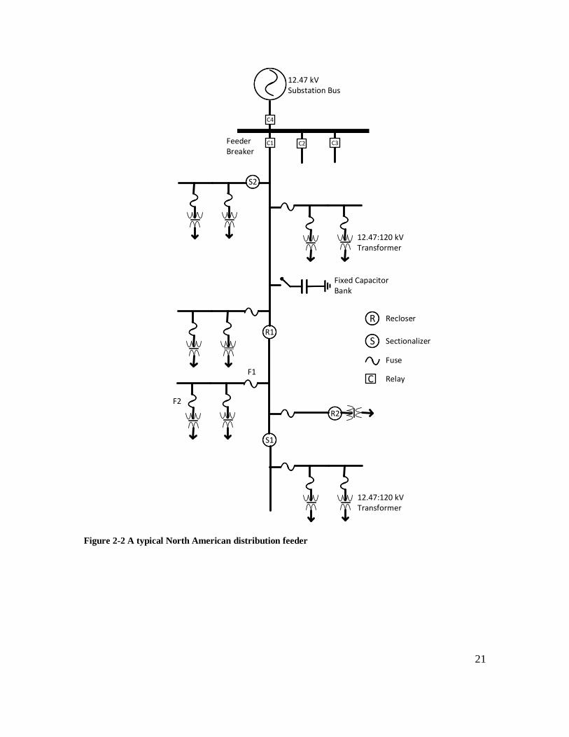
2.3 Operation of reclosers and sectionalizers
A typical North American distribution feeder, including protection devices such as
reclosers, sectionalizers, fuses, and relays, is shown in Figure 2-2[23]. The distribution feeder
shown in Figure 2-2 is a three-phase circuit operating at medium voltage, in this case 12.47 kV. It
is used to describe the interactions between various protection components. This section explains
how the recloser and sectionalizer operate together. As was mentioned in Section 2.2.3, reclosers
can sense and interrupt fault current as well as reclose and re-energize the faulty line. Meanwhile,
sectionalizers are devices capable of isolating faults during the recloser’s dead time and after a
certain number of reclosing operations.
The addition of sectionalizers can improve the protection schemes designed with reclosers.
The distribution feeder in Figure 2-2 is equipped with both reclosers and sectionalizers. The
recloser in the main feeder is set to permit three reclosing operations with the dead times of 0.5s,
10s and 20s respectively. The sectionalizer in the main feeder is set to open after the first reclosing
20
operation. For a fault in-between recloser (R1) and sectionalizer (S1), sectionalizer (S1) does not
observe any fault current through it and will not operate. Thus, in an event of permanent fault in-
between recloser and sectionalizer, the sectionalizer will count all the reclosing instances, yet will
not operate due to not observing any fault current at its location. Eventually, the recloser will
perform three unsuccessful reclosing operations and end up permanently opening the circuit
breaker. In this case, even with the healthy distribution system downstream from the sectionalizer,
loads downstream will experience a power outage.
For a fault downstream from the sectionalizer, it will observe the fault current, hence will
send a signal to open the switch at the location of the sectionalizer during the dead time of the
recloser. Essentially, the traditional recloser-sectionalizer distribution scheme increases the
performance of the distribution system by clearing the permanent faults downstream from the
sectionalizer, without shutting down the entire feeder from the recloser location.
21
Figure 2-2 A typical North American distribution feeder
12.47 kV Substation Bus
C4
C1 C3C2
12.47:120 kV Transformer
Feeder Breaker
S2
Fixed Capacitor Bank
R1
R2
S1
12.47:120 kV Transformer
R
S
Recloser
Sectionalizer
Fuse
C RelayF1
F2

22
2.4 Coordination of various protection devices
Whenever two protection devices happen to be in-between a source and a fault, those
protection devices need to be coordinated in order to isolate the fault with minimum disturbance
to the customers. This section details the basic methods of coordination between different
protection devices in such cases.
2.4.1 Fuse-fuse coordination
Fuses F1 and F2 in Figure 2-2 are in series and it is essential that they are coordinated with
each other. In fuse-fuse coordination, total clearance time for a main fuse (F2) should not exceed
75 percent of the minimum melting time of the backup fuse (F1) for the same current level
[24](𝐹2−𝑇𝐶 < 0.75 ∙ 𝐹1−𝑀𝑀). This ensures that the main fuse interrupts and clears the fault before
the back‐up fuse is affected. The factor of 75 percent compensates for effects such as variations of
load current and ambient temperature, or fatigue in the fuse element caused by the heating effect
of fault currents that have passed through the fuse for an earlier fault instance but not sufficiently
large enough to operate the fuse. Figure 2-3 shows the characteristic curves of the two adjacent
coordinated fuses.

23
Figure 2-3 Fuse-fuse coordination
2.4.2 Recloser-fuse coordination
The criteria for determining recloser‐fuse coordination depend on the relative location of
both devices. If the fuse is located downstream from the recloser as R1 and F1 in Figure 2-2, the
settings must ensure the minimum melting time of the fuse to be greater than the fast curve of the
recloser to keep proper coordination. Furthermore, the total clearing time of the fuse must be
smaller than clearing times obtained with all the slower characteristic curves of the recloser.
Generally, the first opening of a recloser will clear 75 percent of the temporary faults, while the
second will clear another 10 percent. The load fuses are set to operate before the third opening. In
case where the fuse upstream from the recloser, all the recloser operations should be faster than
the minimum melting time of the fuse.
100 1000
1
10
100Ti
me
(s)
Current (A)
F2
F1
F1-MM
F2-TC

24
The operation of fuse-recloser coordination is explained with the fuse recloser pair F1 and
R1 in Figure 2-2. Figure 2-4 shows the time-current characteristic curves associated with both
recloser and the fuse. The recloser is assumed to be set with fast reclosing characteristics curves
followed by two slower reclosing characteristic curves. The fuse is blown only after the first
reclosing action. The slower reclose characteristic curves provide time for the fuse to isolate the
feeder. For fault downstream from F1, for the range of fault currents If (Ifmin < If < Ifmax) the
recloser R1 clears the fault before the fuse is blown. After the first reclosing operation, recloser
operation is switched to the slower characteristic curve. If the fault is still present, fuse F1 will be
blown before the next recloser operation.
Figure 2-4 Fuse-relay coordination
100 1000
1
10
100
Tim
e (
s)
Current (A)
F1
F1-MM
F2-TC
R1-Fa st
R1-Sl ow
Ifmin Ifmax

25
2.4.3 Recloser-relay coordination
An overcurrent relay has an inbuilt time current integration process to determine the
tripping time. During the recloser open time, this process can be result in resetting the time-
overcurrent relay if the line is not re-energized fast enough. If the fault current is re‐applied by
closing the recloser before the overcurrent relay approached complete reset, the overcurrent relay
will at least partially move towards its operating point.
For example, consider a recloser R1 with two fast and two delayed characteristic curves
with reclosing intervals of two seconds. Time-overcurrent relay at C1 has inverse time‐overcurrent
characteristics that takes 0.5s to close its contacts under a certain fault downstream from the
recloser. The overcurrent relay algorithm takes 15s to completely reset the associated integrator.
Coordination should ensure that for a permanent fault downstream from the recloser, the relay
does not completely reset while making sure the relay does not operate until all the recloser
operations are completed.
2.5 Protection of a ring distribution grid structure
The type of protective system and protection devices to protect a distribution grid strongly
depends on the grid structure. A radial distribution grid structure is the most common grid structure
in North America and a ring grid structure more usual in Europe. In Figure 2-5 a typical ring
distribution grid structure is illustrated. The distribution grid is a loop includes a normally open
switch. Normally the switch is open, so two feeders can operate in a radial manner. Feeders are
protected with overcurrent relays located in the main substation. In order to demonstrate the
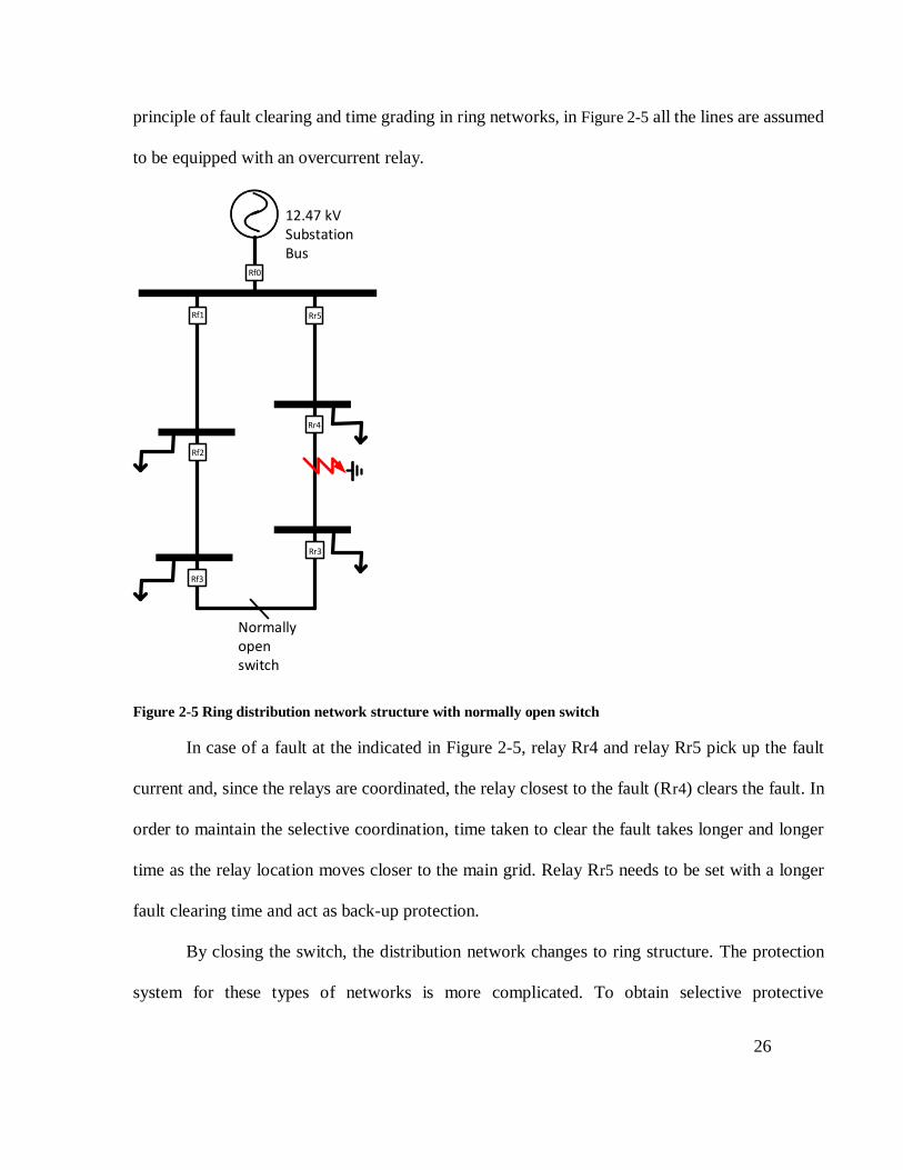
26
principle of fault clearing and time grading in ring networks, in Figure 2-5 all the lines are assumed
to be equipped with an overcurrent relay.
Figure 2-5 Ring distribution network structure with normally open switch
In case of a fault at the indicated in Figure 2-5, relay Rr4 and relay Rr5 pick up the fault
current and, since the relays are coordinated, the relay closest to the fault (Rr4) clears the fault. In
order to maintain the selective coordination, time taken to clear the fault takes longer and longer
time as the relay location moves closer to the main grid. Relay Rr5 needs to be set with a longer
fault clearing time and act as back-up protection.
By closing the switch, the distribution network changes to ring structure. The protection
system for these types of networks is more complicated. To obtain selective protective
12.47 kV Substation Bus
Rf1 Rr5
Rf0
Rf2
Rf3
Rr3
Rr4
Normally open switch
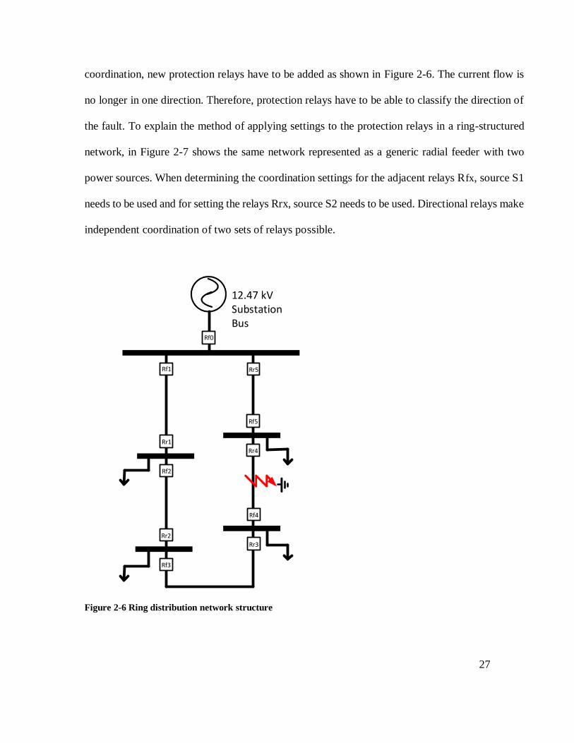
27
coordination, new protection relays have to be added as shown in Figure 2-6. The current flow is
no longer in one direction. Therefore, protection relays have to be able to classify the direction of
the fault. To explain the method of applying settings to the protection relays in a ring-structured
network, in Figure 2-7 shows the same network represented as a generic radial feeder with two
power sources. When determining the coordination settings for the adjacent relays Rfx, source S1
needs to be used and for setting the relays Rrx, source S2 needs to be used. Directional relays make
independent coordination of two sets of relays possible.
Figure 2-6 Ring distribution network structure
12.47 kV Substation Bus
Rf1 Rr5
Rf0
Rr1
Rf2
Rr2
Rf3
Rf4
Rr3
Rf5
Rr4

28
Figure 2-7 Ring network as a radial network with two sources
The fault indicated in Figure 2-7 is fed from both directions and two relays adjacent to the
fault need to operate in order to clear the fault in a selective manner. Relay Rr4 and relay Rr5 detect
the current flow originating from source S1 while the Relay Rf4, relay Rf3, relay Rf2, and relay
Rf1 detects the current flow originating from source S2. In order to maintain the proper
coordination, those two sets of relays need to be coordinated, assuming the radial network
structure. In both sets of relays, relays closest to the sources end up having longer operating times
while the relays further from the source end up having comparatively shorter operating times.
2.6 Protection issues of active distribution networks
Concerns regarding DER integration has been discussed extensively in the literature. There
are three categories of concerns regarding DER integration. Most distribution grid protective
systems detect abnormal network situations by differentiating a fault current from the normal load
current. Inclusion of DER to the distribution network changes both load current and fault current
behaviors of the network. This means, the assumption of unidirectional current flow may not be
valid. Furthermore, the magnitude and duration of the fault current will depend on factors such as
the location of the fault and the type of the DER units involved [7],[9],[14]. Apart from the issues
12.47 kV Substation BusS1
Rr5
Rf4
Rr3Rf5
Rr4
12.47 kV Substation BusS2
29
due to bidirectional current flows, fault currents produced by the DER such as induction generators
and photovoltaic (PV) inverters can be lower in magnitude [25] and temporary. Because of line
and transformer impedance, even the fault currents from small synchronous generators can be
lower in magnitude for faults that are far from the generator. Due to infeed from DER, the fault
current contributions from the utility grid can also be reduced, especially under high impedance
faults. In summary, the addition of DER to the distribution network can cause three types of
protection issues: (i) Change of fault current levels, (ii) change of fault current directions, and (iii)
decreased sustained fault currents [26]. The severity of these impacts depends on a number of
factors. Among these are the type of DER, DER operation mode, interface of DER with power
network and DER capacity, and the structure of the power network. The fault current contribution
from a single smaller DER is not very significant, yet the total contributions of a number of small
units, or a few large units, can change the fault current levels to cause the failure of protective
devices. Following protection problems are discussed in the literature demonstrating the concerns
mentioned above:
Blinding of protection
False tripping
Loss of fuse-recloser coordination
Synchronization issues
Islanding detection
Communication issues
Stability issues
These problems strongly depend on the structure of the distribution network and the type
of DER used. Blinding of protection and false tripping are protection problems that can occur in

30
distribution networks with underground cables as well as overhead lines while fuse-recloser
coordination problems and only appear in distribution networks with overhead lines.
2.6.1 Blinding of protection
Consider the network shown in Figure 2-8. The equivalent circuit during a fault is shown
in Figure 2-9 and the corresponding Thevenin equivalent circuit at the fault location is shown in
Figure 2-10. In Figure 2-9, l is the distance to the DER from the main grid and x is the distance to
the fault from the DER. Z is the impedance per unit length of the distribution line. 𝑍𝐷𝐸𝑅 is the
impedance of the DER and 𝑍𝐺𝑟𝑖𝑑 is the source impedance. The voltages of the DER and main grid
are denoted as 𝑉𝐷𝐸𝑅 and 𝑉𝐺𝑟𝑖𝑑. Equations (2.7) and (2.8) show the relationship between voltages
and currents of the grid and the DER connected to the network. Thevenin impedance and Thevenin
voltage are derived in (2.9)-(2.11). Three-phase fault current and the grid contribution of that fault
current is shown in (2.12)-(2.13). The total short-circuit current (𝐼𝐹𝑎𝑢𝑙𝑡,3𝑝ℎ) is determined by (2.12).
In case of a weak grid, 𝑍𝐺𝑟𝑖𝑑 can be as large as 𝑍𝐷𝐸𝑅 and due to the contribution of the generator,
the grid contribution to the short circuit current decreases.
Overcurrent relays, as well as directional relays, rely on current magnitude exceeding the
pickup current value. Hence, all protective systems based on these protection functions can
malfunction because of the reduced grid contribution. Because of the blinding of protection, there
is a high probability of high impedance faults at the end of the feeder being undetected [27].

31
Figure 2-8 Illustration the effects of blinding of protection for downstream faults
Figure 2-9 Equivalent circuit of Fig 2-8
Figure 2-10 Thevenin equivalent of Fig. 2-9
𝑉𝐺𝑟𝑖𝑑 = 𝐼𝐺𝑟𝑖𝑑(𝑍𝐺𝑟𝑖𝑑 + 𝑧. 𝑙 + 𝑧. 𝑥) + 𝐼𝐷𝐸𝑅 . 𝑧. 𝑥 (2.7)
𝑉𝐷𝐸𝑅 = 𝐼𝐺𝑟𝑖𝑑 . 𝑧. 𝑥 + 𝐼𝐷𝐸𝑅(𝑍𝐷𝐸𝑅 + 𝑧. 𝑥) (2.8)
DER
Relay
Main Grid
I𝐺𝑟𝑖𝑑
I𝐷𝐸𝑅
𝑙 𝑥
I𝐺𝑟𝑖𝑑
𝑉𝐺𝑟𝑖𝑑 , 𝑍𝐺𝑟𝑖𝑑
𝑉𝐷𝐸𝑅 , 𝑍𝐷𝐸𝑅
𝑍𝐷𝐸𝑅
𝑍𝐺𝑟𝑖𝑑 𝑧. 𝑙 𝑧. 𝑥
𝑉𝐺𝑟𝑖𝑑
𝑉𝐷𝐸𝑅
𝑉𝑡ℎ
𝑍𝐷𝐸𝑅
𝑍𝐺𝑟𝑖𝑑 𝑧. 𝑙
𝑧. 𝑥
𝑍𝑡ℎ
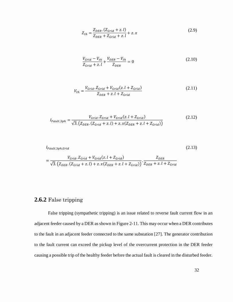
32
𝑍𝑡ℎ =
𝑍𝐷𝐸𝑅 . (𝑍𝐺𝑟𝑖𝑑 + 𝑧. 𝑙)
𝑍𝐷𝐸𝑅 + 𝑍𝐺𝑟𝑖𝑑 + 𝑧. 𝑙+ 𝑧. 𝑥
(2.9)
𝑉𝐺𝑟𝑖𝑑 − 𝑉𝑡ℎ
𝑍𝐺𝑟𝑖𝑑 + 𝑧. 𝑙+
𝑉𝐷𝐸𝑅 − 𝑉𝑡ℎ
𝑍𝐷𝐸𝑅= 0 (2.10)
𝑉𝑡ℎ =
𝑉𝐺𝑟𝑖𝑑 . 𝑍𝐺𝑟𝑖𝑑 + 𝑉𝐺𝑟𝑖𝑑(𝑧. 𝑙 + 𝑍𝐺𝑟𝑖𝑑)
𝑍𝐷𝐸𝑅 + 𝑧. 𝑙 + 𝑍𝐺𝑟𝑖𝑑
(2.11)
𝐼𝐹𝑎𝑢𝑙𝑡,3𝑝ℎ =
𝑉𝐺𝑟𝑖𝑑 . 𝑍𝐺𝑟𝑖𝑑 + 𝑉𝐺𝑟𝑖𝑑(𝑧. 𝑙 + 𝑍𝐺𝑟𝑖𝑑)
√3. (𝑍𝐷𝐸𝑅 . (𝑍𝐺𝑟𝑖𝑑 + 𝑧. 𝑙) + 𝑧. 𝑥(𝑍𝐷𝐸𝑅 + 𝑧. 𝑙 + 𝑍𝐺𝑟𝑖𝑑))
(2.12)
𝐼𝐹𝑎𝑢𝑙𝑡,3𝑝ℎ,𝐺𝑟𝑖𝑑
=𝑉𝐺𝑟𝑖𝑑 . 𝑍𝐺𝑟𝑖𝑑 + 𝑉𝐺𝑟𝑖𝑑(𝑧. 𝑙 + 𝑍𝐺𝑟𝑖𝑑)
√3. (𝑍𝐷𝐸𝑅 . (𝑍𝐺𝑟𝑖𝑑 + 𝑧. 𝑙) + 𝑧. 𝑥(𝑍𝐷𝐸𝑅 + 𝑧. 𝑙 + 𝑍𝐺𝑟𝑖𝑑)).
𝑍𝐷𝐸𝑅
𝑍𝐷𝐸𝑅 + 𝑧. 𝑙 + 𝑍𝐺𝑟𝑖𝑑
(2.13)
2.6.2 False tripping
False tripping (sympathetic tripping) is an issue related to reverse fault current flow in an
adjacent feeder caused by a DER as shown in Figure 2-11. This may occur when a DER contributes
to the fault in an adjacent feeder connected to the same substation [27]. The generator contribution
to the fault current can exceed the pickup level of the overcurrent protection in the DER feeder
causing a possible trip of the healthy feeder before the actual fault is cleared in the disturbed feeder.
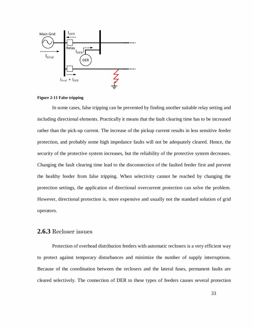
33
Figure 2-11 False tripping
In some cases, false tripping can be prevented by finding another suitable relay setting and
including directional elements. Practically it means that the fault clearing time has to be increased
rather than the pick-up current. The increase of the pickup current results in less sensitive feeder
protection, and probably some high impedance faults will not be adequately cleared. Hence, the
security of the protective system increases, but the reliability of the protective system decreases.
Changing the fault clearing time lead to the disconnection of the faulted feeder first and prevent
the healthy feeder from false tripping. When selectivity cannot be reached by changing the
protection settings, the application of directional overcurrent protection can solve the problem.
However, directional protection is, more expensive and usually not the standard solution of grid
operators.
2.6.3 Recloser issues
Protection of overhead distribution feeders with automatic reclosers is a very efficient way
to protect against temporary disturbances and minimize the number of supply interruptions.
Because of the coordination between the reclosers and the lateral fuses, permanent faults are
cleared selectively. The connection of DER to these types of feeders causes several protection
DER
Relay
Main Grid
I𝐺𝑟𝑖𝑑 I𝐷𝐸𝑅
𝐼𝐺𝑟𝑖𝑑 + 𝐼𝐷𝐸𝑅
I𝐷𝐸𝑅

34
problems at the same time. First, the fault current detection by the recloser is affected by the
generator contribution and can lead to a detection problem. Secondly, the coordination between
reclosers or fuses and reclosers can be lost which directly causes selectivity problems. This is
explained in more detail with the feeders shown in Figure 2-12.
DERRecloser 1
Main Grid
I𝐺𝑟𝑖𝑑
I𝐷𝐸𝑅
I𝐺𝑟𝑖𝑑
DERRecloser 1
Main Grid
I𝐺𝑟𝑖𝑑
I𝐷𝐸𝑅
I𝐺𝑟𝑖𝑑 Recloser 2
Recloser 2
a
b
Figure 2-12 Recloser operation affected by DER
For the shown fault in Figure 2-12(b) short-circuit current measured at Recloser-1 is 𝐼𝐺𝑟𝑖𝑑 .
As demonstrated in section 2.6.1, the contribution to the fault current by the grid decreases and
can result in delays of recloser operation. In the worst case, recloser may not operate at all. For
fault downstream from Recloser-2, the short-circuit current seen by Recloser-2 is (𝐺𝑟𝑖𝑑 + 𝐼𝐷𝐸𝑅),
which is larger than the current sensed by Recloser-1. Most reclosers are equipped with a
dependent time-current characteristic, and the coordination between Recloser-1 and Recloser-2
remains unaffected. Because of the connection of the generator to the feeder, the total short-circuit

35
current is increasing, and for end-of-line faults, the maximum interrupting rating of Recloser-2 has
to be checked.
For the situation in Figure 2-12, the fuse and recloser are coordinated, such that there is
selective fault clearing for the fault currents below maximum fault current. Recloser-1 always
operate before the fuse due to this coordination. When the fault current increases due to the DER
fault current infeed, this coordination no longer holds. The fuse will clear faults before the recloser
operates. Therefore, temporary faults will be cleared permanently and lead to unnecessary
interruptions.
2.6.4 Unnecessary islanding
Islanding is the most discussed issue when adding a DER into a distribution network.
Islanding on a distribution network occurs when a protection device isolates part of the network to
remove a fault while the DER in that section of the network stays online. Due to the various
problems of islanding, which includes the safety of repair personnel, utilities require that DER to
be equipped with anti-islanding protection, DER inside the islanded part of the network should be
disconnected as soon as possible. When a section of a power network is allowed to operate as a
microgrid islanding is not considered as a problem. It is considered as just another operating mode
of the distribution network. However, there needs to be an islanding detection mechanism in order
to change the control and protection settings when an islanding event occurs.
To operate as an island, the protection system needs to detect islands quickly and reliably.
Islanding detection is carried out with passive and active methods [28]. Methods that detect an
islanding event by passively measuring or monitoring the system state are called passive methods.
Under/over voltage protection [29], Under/over frequency protection [29], Voltage Vector Shift

36
(VVS) [30], Rate of change of voltage, Rate of Change of Frequency (ROCOF) [29] and Rate of
change of power [31] are some of the passive methods used for islanding detection. Active methods
are the methods where the detection system is actively interacting with the distribution network in
order to detect islanding operation. Frequency shift method [32], Voltage-pulse perturbation
method [33] and Slip mode frequency shift [32] are active methods of islanding detection found
in the literature.
2.6.5 Synchronization issues
A microgrid needs to be synchronized with the main grid whenever the microgrid
reconnects after a disconnection. The process of synchronization and reconnection may be either
manual or automatic. Synchronizing a microgrid having several generators with different
characteristics is more challenging than synchronizing a single generator with the grid. There are
three main methods of synchronization adopted in active distribution networks: (i) active
synchronization where control mechanism actively controls the voltage, frequency, and phase
angle of the power island to the utility grid, (ii) passive synchronization, where a synchronization
check relay function is utilized, and (iii) open-transition transfer where loads and DER in the island
are disconnected before resynchronization [34]. Both active and passive synchronization schemes
maintain high reliability as compared to the open-transition transfer scheme. Because of the
disconnection of DER from the network, open-transition transfer schemes are not ideal for the
microgrid operation. Active synchronization schemes are more complex and expensive due to the
hardware components required for injecting currents/voltages.
37
2.6.6 Communication issues
Fast and reliable communication is a major issue related to the active distribution network/
microgrid protection scheme design. The knowledge of state of the grid is needed for the smooth
operation of any protection system. Acquiring this knowledge for an active distribution network
requires the application of a fast, reliable and robust communication system with a backup so that
adaptive application of relay setting groups can be done in real-time. The addition of these adaptive
features, which may be needed for the protection of microgrids and active distribution networks,
is a complex and expensive issue. As more and more DER are added to the microgrid, network
protection and control functions become complicated and a reliable and fast communication
medium is a must. IEC 61850 standard has been introduced in cooperation with manufacturers and
users to create a uniform, future proof basis for the protection, communication and control of
substations. IEC 61850 has already gained wide acceptance as the established communication
standard on the worldwide market for the automation of substations and could be one of the
possible frameworks for developing communication solutions needed for the protection of active
distribution networks.
2.6.7 Stability issues
The stability of the microgrid during system fault conditions is also an essential issue in a
microgrid with synchronous generators. Depending on the generator inertia, fault resistance, and
distance to the fault from the generator, the critical clearing times might vary. Fast-acting
protective devices are required to avoid unstable microgrid operation.

38
The reduced fault currents can increase the fault clearing times and therefore affect the
stability of synchronous generators that stay connected to the healthy parts of the network,
including those in the autonomous microgrids that are allowed to be formed consequent to the fault
clearing. This is because small synchronous generators associated with distribution networks are
generally associated with low inertia, high reactance, and poor damping. Synchronous generators
can retain a stable operation only if the rotor angle is kept below a maximum value. Fault clearing
time and generator inertia have important effects on the stability of the synchronous generator.
Fault clearing time for the transmission system can be in the range of 100 ms. However, for
distribution networks, fault clearing time can become much longer.
Moreover, the inertia constant of small synchronous generator is low in comparison with
the inertia constant of about 3–5 s for large synchronous generators. In a distribution network,
keeping the generator connected to the system after a fault is vital for the operation of the
distribution network. Therefore, transient instability becomes a more pressing concern for small
synchronous generators connected to the distribution networks. The loss of synchronism condition
for a synchronous generator is a grave concern for the electrical and mechanical integrity of the
generator.
2.7 Transient stability of synchronous generators
IEEE report “Proposed Terms & Definitions for Power System Stability” [35] defines the
transient stability of a power network as; “A power system is transiently stable for a particular
steady-state operating condition and for a particular large disturbance if, following that
disturbance, it reaches an acceptable steady-state operating condition again”. In the same report,

39
the critical clearing time (CCT) is defined as “the maximum time between the fault initiation and
its clearing such that the power system is transiently stable.”
In distribution networks, the CCT of the integrated synchronous generators can be low due
to the low inertia of the machines, and then the fault clearing process becomes very time-critical.
Therefore, a detailed analysis of the relay timings and communication delays need to be made and
the relay settings need to be determined to avoid violations of CCT of any of the generators
connected to the network. During regular operation, power systems are subjected to small and
large disturbances. An example of a small disturbance is a particular load change, and an example
of large disturbances can be a three-phase fault on a transmission line. To enable security of supply,
power systems have to withstand these kinds of disturbances and stay in stable operation. Transient
stability is the ability of the power system to maintain synchronism when subjected to a severe
transient disturbance the amount of deviation from the steady-state values caused by the
disturbance dependents on factors like type, location, and duration of the disturbance.
To evaluate the stability of a power network, the rotor angle of the generators is often used
as an indicator. The mechanical power of the prime mover cannot change that fast, hence there is
an unbalance between mechanical and electrical power which causes the rotor of the generators to
accelerate. The swing equation (2.14) is used to describe this phenomenon.
2𝐻
𝜔0.𝑑2𝛿
𝑑𝑡2= 𝑃𝑚 − 𝑃𝑒
(2.14)
𝑃𝑚 : Mechanical power in [p.u.]
𝑃𝑒 : Electrical power output in [p.u.]

40
H : Rotor inertia constant in [MW·s/MVA]
𝛿 : Rotor angle in [rad]
𝜔0 : Angular frequency in [rad/s]
t : time in [s]
Neglecting the generator resistance for the generator’s electric power output holds:
𝑃𝑒 =
𝐸𝑞 . 𝑈𝑠
𝑋𝑡. 𝑠𝑖𝑛𝛿 = 𝑃𝑚𝑎𝑥 . 𝑠𝑖𝑛𝛿
(2.15)
Where:
𝐸𝑞 : Generator internal voltage in [p.u.]
𝑈𝑠 : Generator terminal voltage in [p.u.]
𝑋𝑡 : Generator reactance including step-up transformer reactance in [p.u.]
δ : rotor angle in [elect. rad]
Combining equation (2.14) and (2.15) leads to:
2𝐻
𝜔0.𝑑2𝛿
𝑑𝑡2= 𝑃𝑚 − 𝑃𝑚𝑎𝑥 . 𝑠𝑖𝑛𝛿
(2.16)
Using a method such as the equal area criterion, the critical clearing angle can be obtained.
Although this simple method only holds for a single machine system based on a classic generator
model, the analysis provides useful insight into the transient stability problem.
Transient stability mainly depends on, amount of loading at the time of the fault and the
amount of electrical power output during the fault. The rotor inertia is also an important parameter
41
that affects the behavior of the synchronous generator after a fault. The higher the inertia, the
slower the rate of change in the rotor angle.
The fault clearing time determines what the available time is to gain kinetic energy. If this
time is too long, the stability limit of the generator is exceeded, and the generator becomes
unstable. Concerning the transient stability of generators, the fault clearing time is an important
quantity, and the stability limit can be expressed in a critical clearing time (CCT). Clearing time
for a short circuit near the generator terminal can be determined using equation (2.17):
𝑡𝐶𝐶𝑇 = √4𝐻. (𝛿𝑐𝑟 − 𝛿0)
𝜔𝑠 . 𝑃𝑚
(2.17)
where:
𝛿0 : Initial loading [elect. Rad]
𝛿𝑐𝑟 : Critical rotor angle [elect. Rad]
The loss of synchronism is primarily a risk to the generator and is not a serious danger for
the system operation. To prevent transient stability problems, the disconnection of DER,
immediately after the occurrence of a fault is necessary. However, if this DER supplies a
significant share of the total load when operated as a microgrid, disconnection of the DER
following the network faults will remarkably reduce the benefits expected from these energy
sources. In order to keep the generator in operation after a fault, fast clearing of the fault is
necessary to prevent the generator from moving into the unstable region of operation. Also, the
sudden disconnection of a large block of DER could adversely affect the normal operation of the
network. To provide faster fault isolation, protection methods used in traditional distribution
networks require some changes when used in active distribution networks.
42
2.8 Protection methods used in active distribution
networks
2.8.1 Differential protection methods
Few attempts have been made to address the protection issues related to microgird systems
using the differential protection principle [36],[37]. Although differential protection can provide
reliable and fast protection for active distribution systems, implementation of line differential
protection requires a communication infrastructure capable of transferring relatively large amounts
of data between the relays. Differential protection is applied to protect many components within a
power system specially transformers, transmission lines and bus bars [38],[39]. Differential
protection can be considered as a basic application of Kirchhoff’s current law. A differential relay
operates when the sum of currents flowing into a protected segment is not zero, such as a load or
a fault. When there is no net flow of current in or out from the protected segment, the relay will
not operate. Operating margins need to be set to obtain the desired protection function. Most
significant benefit of the implementation of differential protection approaches is that they are not
sensitive to bidirectional power flow and reduction of fault current level of islanded microgrids
[39]. However, some drawbacks associated can be summarized as follows:
In case of communication failure, providing a secondary protection scheme is necessary
Need for expensive communication infrastructure
Unbalanced systems or loads may result in some difficulties in the differential protection
schemes
43
Transients during connection and disconnection of DER may cause some problems for the
operation of the protection system
2.8.2 Impedance based protection methods
The impedance of a line is proportional to its length. Therefore, distance measurement can
be done using a relay capable of measuring the effective impedance. A relay capable of that task
is called a distance relay and is designed to operate only for faults occurring between relay location
and the selected reach point.
In [40][41], a protection strategy based on admittance relays with inverse-time tripping
characteristics is proposed. The relay can distinguish and isolate the faults in both grid-connected
and islanded microgrids. Applicability of this scheme is still not practically validated. Some
challenges associated with the application of these types of relays are identified as follows:
Measurement of the admittance of short lines in distribution networks is challenging
Fault resistance can make errors in the measured admittance
2.8.3 Adaptive protection schemes
The use of adaptive protection schemes that can respond to the changing nature of the
network configurations is another approach to address the protection issues in active distribution
systems. In most of the adaptive protection schemes, protection settings are adjusted when the
network structure is changed. In the protection method proposed in this thesis, adaptive protection
is employed where the protection settings are altered depending on the relative location of the fault
[47].

44
In [68], a new adaptive protection approach has been presented based on the voltage
restrained time overcurrent relays. Although the results are encouraging, the suggested approach
can run into trouble since it has no knowledge about the direction of the fault. Another adaptive
protection scheme, which relies on the dual setting directional overcurrent relays operating in both
forward and reverse directions, has been proposed for a microgrid system in [25]. Although the
proposed scheme is significantly faster than a conventional protection scheme, the use of time
coordination for overcurrent relays has made the overall operation of the protection scheme slower.
The main challenges associated with the implementation of the above-mentioned adaptive
protection techniques are:
The necessity to know all possible states of the microgrid before the implementation
High cost associated with the communication infrastructure.
2.9 Protection algorithms based on transient signals
Conventional power system protection algorithms that operate on the phasor values of the
power frequency currents and voltages have served well over many decades, but with the
increasing penetration of inverter interfaced renewable energy sources [42], they are facing many
challenges, mainly arising from lack of sustained fault current contributions from inverter-
interfaced sources during network faults. These problems are well documented for distribution
networks with DER [43]–[46], but similar problems are appearing in transmission networks as
well with the interconnection of large wind and solar farms [44], [45]. Thus there is renewed
45
interest in transient based and time-domain protection methods [47]–[50] as these techniques are
less dependent on sustained fault currents. Some commercial protection relays based on time-
domain principles are emerging [8]. Protection using transient signals has other advantages such
as fast operation and immunity to current transformer (CT) saturation [51], [52]. There are several
different approaches for transient based protection: traveling-wave based protection [50], [53],
transient directional comparison [54], [55], and differential schemes based on derived quantities
such as transient energy [49]. Traveling wave technique requires precise detection of traveling
wave arrival times at the measurement location [56], while transient directional comparison
techniques need determination of the polarity of the initial transient [54]. Differential techniques,
such as the method presented in [55], usually require a comparison of signal components in a
specific (high) frequency band. The method proposed in [47] does not require any signal
comparisons but relies on the polarity of the transient signals.
Various transient based protection techniques are discussed in the literature. This section
provides a brief overview of such transient based protection techniques. Transient based protection
can be broadly categorized into protection based on incremental signals and protection based on
traveling waves, protection based on signal processing methods and protection based on
differential techniques. There are also instances where a combination of these methods is used.
2.9.1 Protection based on incremental signals
A fault on a transmission line can cause the post-fault voltage and current at the
measurement location to deviate from the steady-state pre-fault voltage and current signals.
Concept for the transient based protection using incremental current and voltage signals is based
on the fact that a fault initiates a voltage/current wave traveling along a transmission line in both

46
forward and backward direction. This incremental signal can be obtained by subtracting the pre-
fault steady-state signals from the measured signals that consist of a fault incident. Common
method used to derive the incremental components is subtracting the value of measured signal
exactly one cycle in the past from the current value of the signal. Another approach is to use high
pass filters to suppress the steady-state signals so that only the transient signals will be present in
the signals. Fault detection and discrimination were achieved using derived incremental
components that are generated due to a fault. A similar method with more detailed explanations is
presented in [57].
Initially, the transient based protection methods were proposed for transmission lines. In
1978 M. Chamia & S. Liberman proposed a transient based protection method for transmission
lines and later became a commercial product. The objective of this research is to substantially
reduce the fault clearing times by identifying the fault faster [58]. This method used a comparison
between the polarities of both initial voltage and current deviations to determine the direction of
the fault. The polarity comparison between both incremental voltage and current waveforms is
carried out separately at each end. The decision is made after exchanging that result via a
communication link. A mathematical explanation of the proposed technique is explained using the
superposition principle. High pass filters are used to obtain the synthesized components needed
for directional comparison.
In [59], before extracting the superimposed transient components, currents, and voltages
are processed to generate necessary signals. The identification of the superimposed signal is
achieved by subtracting the value of processed signal exactly one cycle in the past from the current
value of the processed signal. This technique relies on the trajectory of the current and series of
logic sequences at each end of the protected segment for deriving tripping and blocking commands.
47
The results of a series of laboratory tests are given, and the paper concludes with an illustration of
the performance of the new protection scheme to high resistance single phase to earth faults.
Furthermore, the authors conclude that the performance of the protection scheme depends mainly
on the surge propagation characteristics of a given system rather than on the power frequency
system parameters. This is one of the main advantages when it comes to active distribution system
protection.
In [60], a method in which the fault direction was determined based on the trajectory of the
scaled current deviation ∆𝑖(𝑡) compared to voltage deviation ∆𝑢(𝑡) is presented. Authors suggested
boundaries in (∆𝑢 − 𝑅∆𝑖) plane and initial movement into the first or third quadrant caused by
forward faults and movement to the second and fourth quadrant caused by reverse faults. This
method uses a superposition theorem as in [58] for a mathematical explanation. Unlike [58], this
technique relies on the trajectory of the (∆𝑢 − 𝑘. ∆𝑖) rather than the polarities of ∆𝑢 𝑎𝑛𝑑 ∆𝑖. The
proposed geometric approach is used to extract information on the fault location from the fault
trajectory. Factors that influence the shape of the trajectories are discussed and verified by
numerical simulations and by experiments.
2.9.2 Protection based on traveling waves
Protection of transmission lines using traveling waves of current and voltage signals has
been around for a long time. In 1978, M. Vitinis proposed a method for transmission line protection
using traveling waves [61]. This technique is focussed on determining time delay associated with
the forward and backward traveling waves and use that information to determine the fault location.
Time delay is represented by a rotation/lag of the phasor in the phasor domain. The amount of lag
48
between two phasors is used to calculate the distance to the fault origin. Accuracy of this method
is of the lower end specially when the fault is close to the measurement point.
In [62], the authors propose a distance protection method based on traveling waves.
Correlation between relaying signals (signal representing forward and backward traveling wave
components) is used to determine the fault location. The core principle of this technique is similar
to the technique proposed in [61]. Even with the advanced communication methods available
today, practical application of this method can be challenging due to the fact that decision is based
on the correlation of two time-varying signals at each end of the transmission line.
Reference [54] illustrates the use of directions of current transients to discriminate fault
locations and provide faster and more reliable protection for transmission lines. This protection
scheme shows considerable enhancements of the fault detection and isolation times compared to
the conventional protection methods. The limitation of this protection scheme is the possibility of
malfunction due to any non-fault events that can occur in the power network.
2.9.3 Protection using signal-processing methods
The intelligent protection scheme proposed in [63] combines wavelet transform and
decision trees. Here, the wavelet transform has been used for extracting features for a decision tree
to classify detected faults. However, the decision tree needs to be re-trained if the network
configuration or the operating conditions are substantially changed. In [64], a differential
protection scheme that operates based on the differential energy calculated using the S-transform
has been presented for a microgrid system. Although the results showed acceptable operating
speed (four cycles) from the fault inception, the possibility of mal-operation due to transients

49
originating from non-fault related events can be considered as one of the shortcomings of this
method.
In [65], a traveling wave-based protection scheme has been proposed for an inverter
dominated microgrid system. This scheme utilizes an improved mathematical morphology (MM)
technique to determine the transient polarity. Trip decision by the protection is taken with the
knowledge of fault location. This paper also focuses on essential aspects such as signal processing
and the effects of noise.
Reference [66] presents a new high-speed protection scheme for power transmission lines
using wavelet transformation. In this protection scheme, fault-generated high-frequency transient
signals contained in the primary voltages are utilized to detect fault position according to their
relative traveling time and polarities. Using the wavelet transform (Morlet wavelet, 80kHz), the
time of the reflections is obtained with high accuracy. That timing information is used to determine
the location of the fault. Information obtained from complex wavelet coefficients are used to
extract and localize a band of specified high-frequency components propagating along the
transmission line. Fault classification is not addressed in the paper. Furthermore, reflection
sequences caused by multi-reflections can cause issues with the proposed scheme.
Reference [67] describes a novel technique for current differential pilot relay protection by
using wavelet analysis. Power system simulation software (PSCAD) is used to generate current
signals at both ends of a transmission line in a typical system with faults at various locations.
Discriminating between internal fault and external fault/change, identifying of faulted phase, and
classifying fault type are achieved by using wavelet analysis.
Although these transient based protection methods have shown promising results, their
practical application is hindered by factors such as bandwidth limitations of the conventional

50
sensors, need for hardware capable of high speed signal processing, possibility of not generating
a transient signal when a fault initiated at the current zero-crossing and the inability of completely
preventing false tripping due to non-fault transients.
51
Chapter 3
Development of a sensor for detecting
current transient polarities
3.1 Introduction
Chapter 2 provided a short description of transient based protection methods proposed for
distribution networks. A group of transient based protection methods uses polarity of the current
or/and voltage transients to determine the relative location of the fault. The hybrid protection
method proposed in this thesis also uses current transient polarities for the determination of relative
fault location. The determination of transient polarities for protection applications is a challenging
task due to the time constraints involved, and a novel sensor is proposed for this purpose in this
Chapter. The content of this chapter is based on the original work published in;
A. Pathirana, C. K. G. Piyadasa, A. D. Rajapakse “Development and modeling of a new type of
sensor for detecting current transients for power system protection,” International Journal of
Electrical Power and Energy Systems 101, 243-254, 2018 [69].
3.2 Detection of polarity of transients
Some of the approaches that have been proposed for the detection of the polarity of
transient signals are discussed below.

52
3.2.1 Signal processing methods
Signal processing methods are used to enhance the visibility of the transient event and
capture the transient polarity. The general approach of this method is to sample the voltage and/or
current signals at a frequency much higher than the frequency of the targeted transient signals and
apply signal processing techniques for the determination of the polarity. For example, digital
filters, wavelet transform, and mathematical morphology are used as signal processing methods.
Table 3-1 summarises some of the transient based protection methods that use polarity of the
current/voltage signal to identify the relative fault location and respective signal processing
methods used by the proposed methodology. These transient based protection methods that rely
on the polarity of the transient signals or the time of arrival of the transmitted/reflected traveling
waves, accurate measurement of the current waveform is not necessary, but accurate detection of
high-frequency transients with minimal rise time is essential.
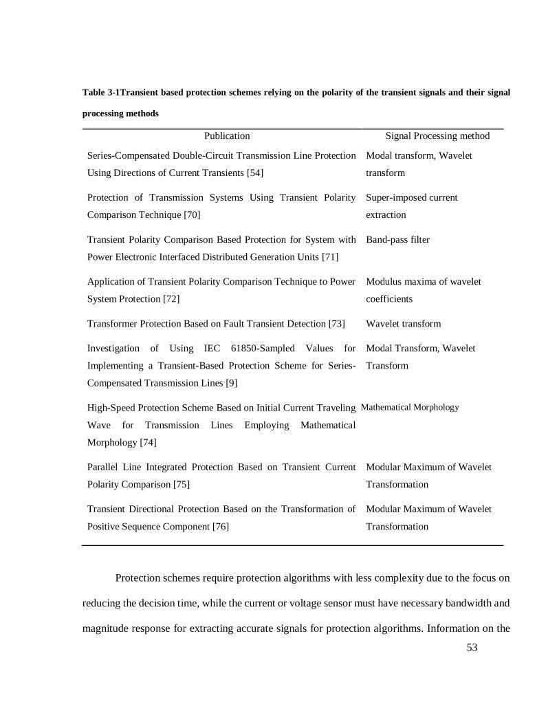
53
Table 3-1Transient based protection schemes relying on the polarity of the transient signals and their signal
processing methods
Publication Signal Processing method
Series-Compensated Double-Circuit Transmission Line Protection
Using Directions of Current Transients [54]
Modal transform, Wavelet
transform
Protection of Transmission Systems Using Transient Polarity
Comparison Technique [70]
Super-imposed current
extraction
Transient Polarity Comparison Based Protection for System with
Power Electronic Interfaced Distributed Generation Units [71]
Band-pass filter
Application of Transient Polarity Comparison Technique to Power
System Protection [72]
Modulus maxima of wavelet
coefficients
Transformer Protection Based on Fault Transient Detection [73] Wavelet transform
Investigation of Using IEC 61850-Sampled Values for
Implementing a Transient-Based Protection Scheme for Series-
Compensated Transmission Lines [9]
Modal Transform, Wavelet
Transform
High-Speed Protection Scheme Based on Initial Current Traveling
Wave for Transmission Lines Employing Mathematical
Morphology [74]
Mathematical Morphology
Parallel Line Integrated Protection Based on Transient Current
Polarity Comparison [75]
Modular Maximum of Wavelet
Transformation
Transient Directional Protection Based on the Transformation of
Positive Sequence Component [76]
Modular Maximum of Wavelet
Transformation
Protection schemes require protection algorithms with less complexity due to the focus on
reducing the decision time, while the current or voltage sensor must have necessary bandwidth and
magnitude response for extracting accurate signals for protection algorithms. Information on the
54
practical implementation issues and the limitations related to signal acquisition and conditioning
are rare in the published literature [52]. High frequency, high precision sampling, and thus
expensive analog to digital (A/D) converters is one of the limitations with the signal processing
methods [53].
3.2.2 Measurement of transients
In some cases, the limited bandwidth of conventional CTs and voltage transformers (VTs)
can become critical to the performance of polarity determination. Conventional current
transformers (CTs) used for current measurements in power networks may not be adequate for
measuring high-frequency transients due to limited bandwidth, and the dispersion of transient
signal due to secondary leakage [51], [77].
For current transient measurements, there are several available measurement methods. One
of the simplest and common ones is to use a shunt resistor connected in series on the power line
being measured, which then provides a voltage signal proportional to the current measured;
however, this is rather expensive for high-voltage applications. Generally, in substations, feeder
currents are measured using iron-core current transformers. These current transformers have
relatively low bandwidth. For broader bandwidth measurements, several other solutions are
available. Devices based on Hall effect are making their way into high-voltage measurement
systems [78]. Hall-effect is feasible as it allows miniature sensors with rather good performance,
but they need power supply and are somewhat expensive in high-voltage applications. Another
way is the use of fully optical effect current sensors, employing measurement of the Faraday effect
to determine the current value [79]. The optical transducers once again are more expensive, as they
require precise lasers for providing accurate measurements. Rogowski coils have been utilized for
55
power frequency and transient current measurements due to their high bandwidth, linearity, and
ability to measure large currents [80]. Since there are no magnetic materials in the flux path, output
voltages are quite low relative to the conventional CTs. A few authors have proposed the use of
open-circuited coils similar to Rogowski coils but wound on ferrite cores [10]–[12] for transient
detection. However, these publications provide only limited insight into theoretical aspects and
mathematical modeling of the sensor.
The following sections introduces a sensing system designed for precisely determining the
polarity of the initial momentary change of current. The hybrid protection scheme proposed in
Chapter 4 uses this sensor to detect the current transient polarity. The next section details the design
and operation of the proposed current transient sensor. Later in the chapter, sensor operation is
verified with laboratory experiments.
3.3 Design and operation of the current transient
sensor
This section describes the proposed sensing system designed for the detection of current
transients. The primary component of the sensing system is a simple detection coil wound on a
ferrite core. Initially, experiments are carried out to understand this behavior and it shows ferrite
core coil can be used to detect the high-frequency transients, even with the core saturated due to
low-frequency currents. Moreover, the proposed sensing system replaces both high-frequency
signal sampling and processing by a simple detection coil wound on a ferrite core and an analog
electronic circuit. Laboratory experiments are used to verify that the ferrite core coil is capable of
detecting transient occurrence and initial transient polarity accurately. Transient detection using

56
ferrite-cored coils can lead to accurate fault location and protection solutions based on the detection
of initial transients. In order to use the ferrite core coil sensor in EMT (Electro-Magnetic Transient)
simulations, a mathematical model of the proposed ferrite cored coil is formulated. This
mathematical model is verified through laboratory experiments.
Figure 3-1 illustrates the components of the proposed sensor system designed to detect the
initial polarity of current transients after a fault. The sensor system takes the monitored current as
input and outputs the initial polarity of the current transient. The input to the sensor system can
either be a current flowing in a high voltage conductor or a current on the secondary of an already
installed conventional current transformer (CT).
Figure 3-1 Current transient polarity detection sensor
Primary current of the ferrite core coil is the input to the sensor system. In this
implementation, the ferrite core coil is inserted into the secondary of installed CT. That is due to
the practical considerations but it is preferred to give the line current as the input to the ferrite core
coil. When the input to the sensor system is the secondary current of CT, the required insulation

57
levels are reduced, and the whole sensor can be mounted inside a commercially available digital
protection relay. When the sensor system is directly connected to the high voltage conductor, the
necessary insulation must be provided between the conductor and the ferrite core coil, which is
similar to a conventional CT.
The induced voltage of the ferrite core coil is fed to the next stage of the sensor system
which is the protection circuit. This protection circuit prevents possible damage to the electronic
circuits of the sensor system from excessive transient currents and transient voltages. The
protection circuit consists of a fuse and Zenner diodes for protecting from current and voltage
transients, respectively.
A passive high pass filter is added as the next stage to remove low-frequency currents and
their harmonics. Saturation causes the induced voltages to have a distorted waveform, resulting in
a significant amount of lower-order harmonics. The cut-off frequency of the high pass filter was
set to 1 kHz to block the power frequency signals and lower order harmonics of the power
frequency. A low pass filter is included after the high pass filter to remove the undesirable high-
frequency components of the output voltage waveform. The cut-off frequency of the low pass filter
is set to 200 kHz. Since the ferrite coil is constructed with only a few secondary turns, self-
inductance, and capacitance of the ferrite coil will be very small, and therefore the upper limit of
coil bandwidth is imposed by the frequency response of the ferrite core. This limit is in the range
of several MHz for conventional ferrite materials [81]. In case the low pass filter is not included
in the sensor system, the upper limit of the frequency range of the sensing system is only restricted
by the frequency response of the ferrite core coil. However, when the ferrite core is mounted on
the secondary of a CT, the highest frequency will be determined by the CT bandwidth.
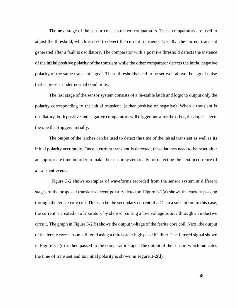
58
The next stage of the sensor consists of two comparators. These comparators are used to
adjust the threshold, which is used to detect the current transients. Usually, the current transient
generated after a fault is oscillatory. The comparator with a positive threshold detects the instance
of the initial positive polarity of the transient while the other comparator detects the initial negative
polarity of the same transient signal. These thresholds need to be set well above the signal noise
that is present under normal conditions.
The last stage of the sensor system consists of a bi-stable latch and logic to output only the
polarity corresponding to the initial transient. (either positive or negative). When a transient is
oscillatory, both positive and negative comparators will trigger one after the other, this logic selects
the one that triggers initially.
The output of the latches can be used to detect the time of the initial transient as well as its
initial polarity accurately. Once a current transient is detected, these latches need to be reset after
an appropriate time in order to make the sensor system ready for detecting the next occurrence of
a transient event.
Figure 3-2 shows examples of waveforms recorded from the sensor system at different
stages of the proposed transient current polarity detector. Figure 3-2(a) shows the current passing
through the ferrite core coil. This can be the secondary current of a CT in a substation. In this case,
the current is created in a laboratory by short-circuiting a low voltage source through an inductive
circuit. The graph in Figure 3-2(b) shows the output voltage of the ferrite core coil. Next, the output
of the ferrite core sensor is filtered using a third-order high pass RC filter. The filtered signal shown
in Figure 3-2(c) is then passed to the comparator stage. The output of the sensor, which indicates
the time of transient and its initial polarity is shown in Figure 3-2(d).
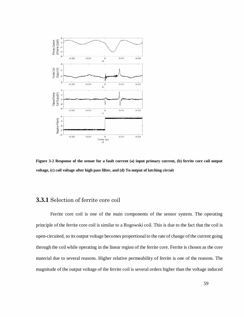
59
Figure 3-2 Response of the sensor for a fault current (a) input primary current, (b) ferrite core coil output
voltage, (c) coil voltage after high pass filter, and (d) Tn output of latching circuit
3.3.1 Selection of ferrite core coil
Ferrite core coil is one of the main components of the sensor system. The operating
principle of the ferrite core coil is similar to a Rogowski coil. This is due to the fact that the coil is
open-circuited, so its output voltage becomes proportional to the rate of change of the current going
through the coil while operating in the linear region of the ferrite core. Ferrite is chosen as the core
material due to several reasons. Higher relative permeability of ferrite is one of the reasons. The
magnitude of the output voltage of the ferrite coil is several orders higher than the voltage induced

60
on a Rogowski coil, which has air as the magnetic medium. Due to this fact, the design of the
sensing coil requires a fewer turns, thereby reducing its self-inductance. However, to design a coil
that operates only in the linear region of the core characteristics requires a ferrite core with a large
cross-section area, making the sensor bulky. Laboratory experiments show that current transients
can be successfully detected even when the core is in saturation. Section 3.3.2 discusses this
experiment in detail.
Furthermore, compared to other metal alloys, ferrite performs better under magnetic fields
of higher frequencies. This is due to significant oxygen ions presence in the crystal lattice of
ferrites. These oxygen ions act as an insulator and increase the resistivity to the magnetic flux.
This property makes the ferrite especially useful at higher frequencies since it causes a lesser
amount of losses compared to magnetic materials such as metals and metal alloys.
3.3.2 Comparison with other core types
This section compares the ferrite core coil with other possible core types, namely,
Rogowski coils and iron cored coils. The simple test setup shown in Figure 3-3 is designed to
investigate the response of the ferrite-cored coil compared to the Rogowski coil and iron cored
coil for high-frequency transients. A current amplifier is used to inject power frequency currents
through the primary circuit. A charged capacitor connected in series with a resistor and switch is
used to inject the transient signals, as the bandwidth of the current amplifier was not sufficient to
inject high-frequency transients. The capacitor is pre-charged to the required voltage, and the
switch is closed to inject the transient current into the power frequency current signal generated
by the current amplifier. The high bandwidth current probe used for measuring the primary current

61
utilized Hall Effect sensors. Output voltages of the ferrite core coil, Rogowski coil, and iron core
coil, as well as the primary current, were measured using an oscilloscope.
Current
Amplifier
1 Ω
Ferrite core coil
Switch
Hall effect
sensor
3 . 2 mF
Oscillo
sco
pe
Iron core coil
Rogowskicoil
+
-
Figure 3-3 Experimental setup designed to compare different core types
Figure 3-4 displays the responses of the three coils and the corresponding primary current.
Due to the high permeability of the ferrite core, significantly high output voltage magnitude can
be observed from the ferrite core coil. Ferrite core coil response has a peak of six volts. This is
significantly high compared to the output voltages of the Rogowski coil (peak of 20 mV) and iron
core coil (peak of 0.5 V). Apart from the peak magnitude, Ferrite cored coil output displays much
better slew rate compared to iron core coil, making the ferrite core coil the most suitable approach
to detect polarities of current transients.

62
Figure 3-4 Output voltage response of different core types while the core is unsaturated
The next part of the experiments is carried out to investigate whether a ferrite core coil can be used
to detect the high-frequency transients when the core is saturated due to low-frequency currents.
To test the performance of the ferrite cored coil under the condition of core saturation, the same
test up used in the previous experiment was used with a DC shift in the injected primary current.
Figure 3-5 shows the responses from the three coils and the corresponding primary current. The

63
DC shift given to the primary current saturated the core of the ferrite core. Even in this case, the
ferrite core coil generates significantly high output voltage compared to the Rogowski coil. Even
the slew rate of the ferrite core coil is observed to be higher than that of the Rogowski coil. This
result shows being partially saturated due to the low frequency or DC does not cripple the ferrite
core from generating a response to a high-frequency transient.
Figure 3-5 Response to transient currents when the ferrite core is saturated
The frequency response of the ferrite core is not the only factor affecting the bandwidth of
the sensor. The self-inductance and the resistance of the secondary coil limit the bandwidth and
slew rate of the sensor. In a Rogowski coil, where the core has no frequency dependence, the self-

64
inductance and the resistance of the coil are the factors that limit the bandwidth and slew rate. For
comparison, consider a ferrite core coil designed to have the same output voltage as a Rogowski
coil for a given primary current. For the two sensors, the relationship in (3. 1) can be obtained.
𝜇𝑜 . 𝐴.𝑁𝑟𝑜𝑔
𝑙.𝑑(𝐼𝑝)
𝑑𝑡= 𝜇𝑓𝑒𝑟𝑟𝑖𝑡𝑒 . 𝐴.
𝑁𝑓𝑒𝑟𝑟𝑖𝑡𝑒
𝑙.𝑑(𝐼𝑝)
𝑑𝑡 (3.1)
Where μo is the permeability of air, μferrite is the permeability of ferrite core, and Nrog and
Nferrite are the number of turns on the Rogowski coil and the ferrite core coil, respectively. The
relationship in (3.1) can be reduced to;
𝑁𝑟𝑜𝑔
𝑁𝑓𝑒𝑟𝑟𝑖𝑡𝑒=
𝜇𝑓𝑒𝑟𝑟𝑖𝑡𝑒
𝜇𝑜 (3.2)
The effective permeability of a ferrite core is several orders more significant than the
permeability of air. Therefore, the number of turns required in the Rogowski coil to produce the
same output would be very high. The self-inductance of a coil is directly proportional to the
permeability and the square of the number of turns. The ratio of inductance for this case can be
written as (3.3). Equation (3.3) can be reduced to (3.4) by substituting from (3.2), the result gives
an interesting insight into the comparison with Rogowski coil.
𝐿𝑟𝑜𝑔
𝐿𝑓𝑒𝑟𝑟𝑖𝑡𝑒=
𝜇𝑜. 𝑁𝑟𝑜𝑔2
𝜇𝑓𝑒𝑟𝑟𝑖𝑡𝑒 . 𝑁𝑓𝑒𝑟𝑟𝑖𝑡𝑒2 (3.3)
65
𝐿𝑟𝑜𝑔
𝐿𝑓𝑒𝑟𝑟𝑖𝑡𝑒=
𝜇𝑓𝑒𝑟𝑟𝑖𝑡𝑒
𝜇𝑜 (3.4)
Permeability of ferrite coil (𝜇𝑓𝑒𝑟𝑟𝑖𝑡𝑒) is significantly larger than the permeability of
Rogowski coil (𝜇𝑜). According to (3.4), the sensor with a ferrite core coil will have a much lower
self-inductance compared to an air-cored Rogowski coil when the input current and output voltage
is similar. This is one of the main advantages of the proposed new sensor in transient detection
applications.
In order to use the ferrite core coil sensor in the EMT simulation platform, a mathematical
model of the ferrite core coil needs to be formulated. As a subsequent step, a mathematical model
is developed for the ferrite core coil to facilitate simulating the sensor system.
3.4 Mathematical model of ferrite core sensor
Field-testing of new or existing protection algorithms is not a practical solution. Therefore,
power utilities and researchers use computer simulations to evaluate the performance of protection
algorithms. In the field of power systems, EMT simulation programs are often used for verifying
protection algorithms. For example, the well-known EMT program PSCAD, and its extensive
master library contains most of the power system and control system component models required
for the simulation of electrical power networks and their protection schemes. Simulations in EMT
simulation program (PSCAD), facilitates testing the application of the designed sensor system for
protection applications. The existing Master Library components of PSCAD can be used to
simulate most parts of the sensor system except the ferrite-cored coil. Therefore, a simulation
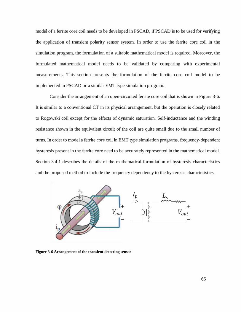
66
model of a ferrite core coil needs to be developed in PSCAD, if PSCAD is to be used for verifying
the application of transient polarity sensor system. In order to use the ferrite core coil in the
simulation program, the formulation of a suitable mathematical model is required. Moreover, the
formulated mathematical model needs to be validated by comparing with experimental
measurements. This section presents the formulation of the ferrite core coil model to be
implemented in PSCAD or a similar EMT type simulation program.
Consider the arrangement of an open-circuited ferrite core coil that is shown in Figure 3-6.
It is similar to a conventional CT in its physical arrangement, but the operation is closely related
to Rogowski coil except for the effects of dynamic saturation. Self-inductance and the winding
resistance shown in the equivalent circuit of the coil are quite small due to the small number of
turns. In order to model a ferrite core coil in EMT type simulation programs, frequency-dependent
hysteresis present in the ferrite core need to be accurately represented in the mathematical model.
Section 3.4.1 describes the details of the mathematical formulation of hysteresis characteristics
and the proposed method to include the frequency dependency to the hysteresis characteristics.
Figure 3-6 Arrangement of the transient detecting sensor
𝐿𝑠 𝐼𝑝
𝑉𝑜𝑢𝑡 𝑉𝑜𝑢𝑡

67
3.4.1 Modeling of hysteresis of the ferrite core
The Jiles-Atherton (JA) theory [82] is the primary method used to formulate the dynamic
characteristics of magnetic materials. It presents a quantitative model of hysteresis phenomena in
magnetic materials and mimics all of the main behaviors of hysteresis characteristics such as the
initial magnetization curve, saturation of magnetization, coercivity, remanence, and hysteresis
loss. Therefore, the JA model is chosen as a suitable mathematical model to represent ferrite core
characteristics.
JA theory describes the hysteresis of a magnetic material by transforming the relationship
between the magnetic flux density (B) and the magnetic field strength (H) into a relationship
between the magnetic moment (M) and the effective field (𝐻𝑒). These relationships are shown in
(3.5) and (3.6):
𝐵 = 𝜇0(𝐻 + 𝑀) (3.5)
𝐻𝑒 = 𝐻 + 𝛼𝑀 (3.6)
where 𝛼 represents the inter-domain coupling interaction. The anhysteretic
magnetization𝑀𝑎𝑛, can be expressed in the form given in (3.7), where 𝑀𝑆𝑎𝑡 is the saturation
magnetization and f() is an arbitrary function of the effective field.
𝑀𝑎𝑛 = 𝑀𝑆𝑎𝑡𝑓(𝐻𝑒) (3.7)
JA model uses a modified Langevin function to represent 𝑓(𝐻𝑒) as given in (3.4), where
the parameter (A) is used to define the shape of the model.
𝑓(𝐻𝑒) = 𝑐𝑜𝑡ℎ (
𝐻𝑒
𝐴) −
𝐴
𝐻𝑒
(3.8)

68
According to the JA theory, magnetic moment (M) consists of two components as shown
in (3.9) where 𝑀𝑖𝑟𝑟𝑒𝑣 represents the pinning of the magnetic domains by discontinuities in the
material structure and 𝑀𝑟𝑒𝑣𝑠 represents the domain wall bending in an elastic manner.
𝑀 = 𝑀𝑖𝑟𝑟𝑒𝑣 + 𝑀𝑟𝑒𝑣𝑠 (3.9)
Then the relationship between M and H can be expressed using the differential equations
given in (3.10) and (3.11) as proposed in [83], where 𝑐 is called the domain flexing parameter, and
𝛿 is a variable that indicates whether the magnetic field is increasing or decreasing.
𝑑𝑀
𝑑𝐻=
𝑐𝑑𝑀𝑎𝑛𝑑𝐻𝑒
+𝑀𝑎𝑛 − 𝑀
𝛿𝑘𝜇0
−𝛼(𝑀𝑎𝑛 − 𝑀)
1 − 𝑐
1 − 𝛼𝑐𝑑𝑀𝑎𝑛𝑑𝐻𝑒
for all (𝑀𝑎𝑛 − 𝑀)𝛿 > 0
(3.10)
𝑑𝑀
𝑑𝐻=
𝑐𝑑𝑀𝑎𝑛𝑑𝐻𝑒
1 − 𝛼𝑐𝑑𝑀𝑎𝑛𝑑𝐻𝑒
for all (𝑀𝑎𝑛 − 𝑀)𝛿 < 0
(3.11)
Where,
𝛿 = 1𝑖𝑓𝑑𝐻
𝑑𝑡> 1
𝛿 = −1𝑖𝑓𝑑𝐻
𝑑𝑡< 1
A, α, c and k are constants for the material being used and can be determined using
measured hysteresis curves and curve-fitting techniques. Details of the approach for parameter
evaluation are discussed in [83].

69
3.4.2 Inclusion of dynamic behavior
The hysteresis model described by (3.5)-(3.11) is static and mainly used for describing the
power frequency behavior of ferromagnetic materials. It does not represent the frequency-
dependent or dynamic behavior of hysteresis characteristics. The designed sensor is targeted for
detecting high-frequency transients, and therefore, the high-frequency behavior of the core
material should be accurately modeled in the simulation model. In order to model the dynamic
behavior and the resulting variations in the energy losses in the core, the JA model needs to be
extended. The dynamic behavior can be included in various ways. For example, in [84], a term
proportional to 𝑑𝐵
𝑑𝑡 is added to (3.10) and (3.11). Reference [84] achieves the dynamic behavior by
dividing the static 𝑑𝑀
𝑑𝐻 by a dynamic factor proportional to
𝑑𝐵
𝑑𝑡. Furthermore, in [84], it is shown that
a dynamic factor proportional to 𝑑𝐻
𝑑𝑡 gives a better fit to experimental data than the term
proportional to 𝑑𝐵
𝑑𝑡. Apart from that, the natural independent variable of the data is H. Therefore, it
is straightforward to adopt H as the independent variable for the dynamic model rather than B.
After a comparison of different approaches, it was found that the latter model gives a good
representation of high-frequency excitations while retaining the ability to represent static
magnetization. Thus, (3.10) and (3.11) were modified to incorporate dynamic behavior as shown
in (3.12)
(𝑑𝑀
𝑑𝐻)
𝑑𝑦𝑛𝑎𝑚𝑖𝑐=
(𝑑𝑀𝑑𝐻
)𝑠𝑡𝑎𝑡𝑖𝑐
1 + 𝑅𝑑𝐻𝑑𝑡
(3.12)
The factor R is a material property and can be determined experimentally using curve fitting
with measured high-frequency hysteresis curves, as discussed in [84].

70
3.4.3 EMT simulation model of the ferrite core coil
When modeling open-circuited ferrite core coil in an EMT simulation program, it is
necessary to determine the change in secondary voltage for a given change in primary current in
each simulation time interval, ∆𝑡. Such a model can be developed from basic principles. Applying
Ampere’s law to the core of the coil shown in Figure 3-6.
∆𝐻 =
𝑁𝑝
𝑙∆𝐼𝑝
(3.13)
where 𝑁𝑝 is the number of turns in the primary; l is the length of the flux path, ∆𝐻 is the
change in magnetic field strength and ∆𝐼𝑝is the change in primary current, which is the excitation
given to the model. In the proposed sensor, the coil output is connected to a voltage measurement
circuit, thus the secondary current, 𝐼𝑠 is assumed to be negligible. Therefore, the output voltage,
𝑉𝑜𝑢𝑡 is obtained as;
𝑉𝑜𝑢𝑡 =
𝑁𝑠𝐴𝑐
∆𝑡∆𝐵 (3.14)
The value of ∆𝐵 can be calculated by solving (3.5)-(3.12), with ∆𝐻 obtained from (3.13).
These equations are solved in each time step to determine the three unknowns ∆𝐻, ∆𝑀 and ∆𝐵 to
be used in the next time step. Finally, ∆𝐵 can be used to determine the output voltage of the ferrite
core coil, according to (3.14). This procedure was implemented through a user-defined model in
EMT simulation software PSCAD. As the model is highly nonlinear, precautions need to be taken
to maintain the numerical stability by selecting the appropriate simulation time step.
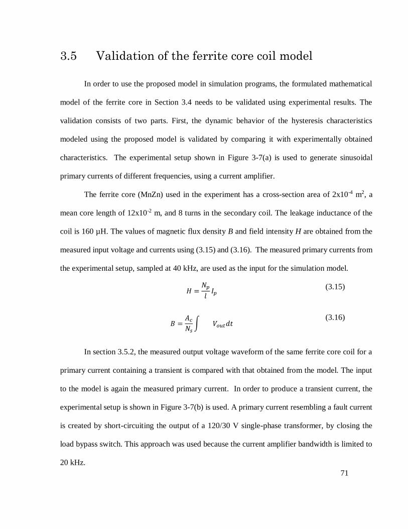
71
3.5 Validation of the ferrite core coil model
In order to use the proposed model in simulation programs, the formulated mathematical
model of the ferrite core in Section 3.4 needs to be validated using experimental results. The
validation consists of two parts. First, the dynamic behavior of the hysteresis characteristics
modeled using the proposed model is validated by comparing it with experimentally obtained
characteristics. The experimental setup shown in Figure 3-7(a) is used to generate sinusoidal
primary currents of different frequencies, using a current amplifier.
The ferrite core (MnZn) used in the experiment has a cross-section area of 2x10⁻⁴ m2, a
mean core length of 12x10-2 m, and 8 turns in the secondary coil. The leakage inductance of the
coil is 160 µH. The values of magnetic flux density B and field intensity H are obtained from the
measured input voltage and currents using (3.15) and (3.16). The measured primary currents from
the experimental setup, sampled at 40 kHz, are used as the input for the simulation model.
𝐻 =
𝑁𝑝
𝑙𝐼𝑝
(3.15)
𝐵 =
𝐴𝑐
𝑁𝑠∫ 𝑉𝑜𝑢𝑡𝑑𝑡
(3.16)
In section 3.5.2, the measured output voltage waveform of the same ferrite core coil for a
primary current containing a transient is compared with that obtained from the model. The input
to the model is again the measured primary current. In order to produce a transient current, the
experimental setup is shown in Figure 3-7(b) is used. A primary current resembling a fault current
is created by short-circuiting the output of a 120/30 V single-phase transformer, by closing the
load bypass switch. This approach was used because the current amplifier bandwidth is limited to
20 kHz.
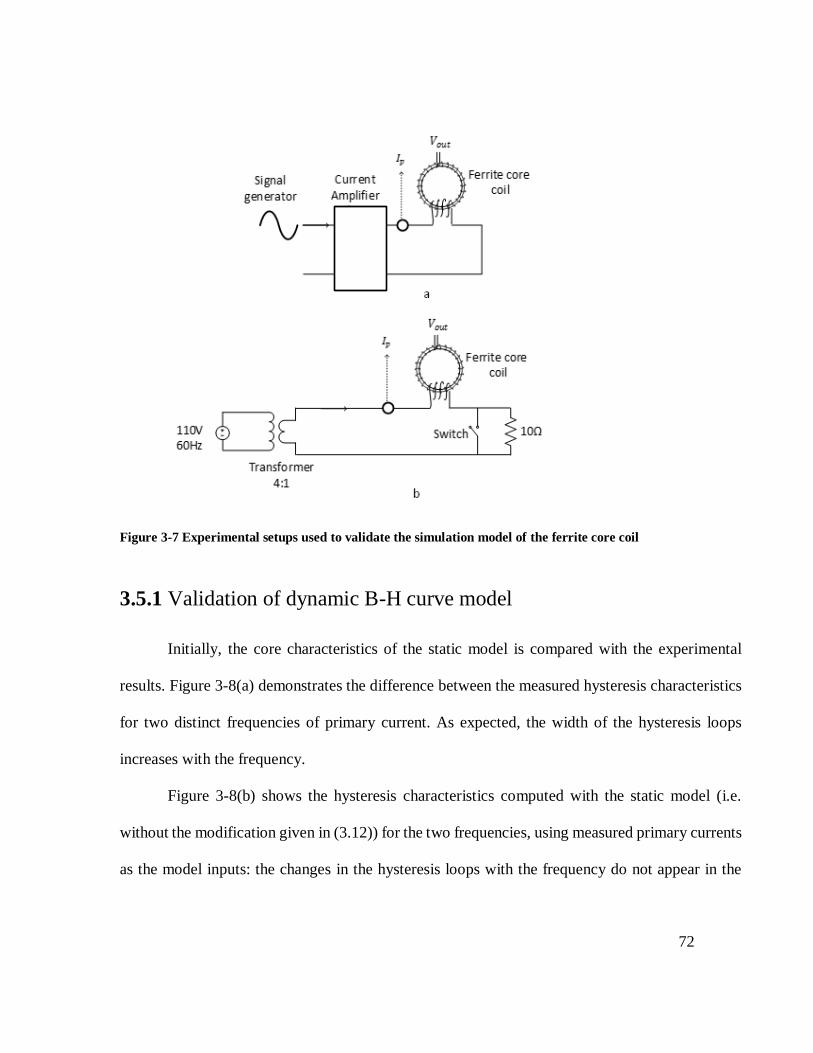
72
Figure 3-7 Experimental setups used to validate the simulation model of the ferrite core coil
3.5.1 Validation of dynamic B-H curve model
Initially, the core characteristics of the static model is compared with the experimental
results. Figure 3-8(a) demonstrates the difference between the measured hysteresis characteristics
for two distinct frequencies of primary current. As expected, the width of the hysteresis loops
increases with the frequency.
Figure 3-8(b) shows the hysteresis characteristics computed with the static model (i.e.
without the modification given in (3.12)) for the two frequencies, using measured primary currents
as the model inputs: the changes in the hysteresis loops with the frequency do not appear in the

73
simulated curves. The model parameters for these curves are obtained using measurements made
at 50 Hz.
Figure 3-8 Experimental results illustrating the dynamic behaviour of the B-H curve (b) Simulation results
with static B-H curve model

74
Figure 3-9 Simulation results with the dynamic B-H curve model
Figure 3-9 demonstrates B-H curves obtained with the dynamic model of hysteresis
characteristics for the same primary current inputs. Modification proposed in (3.12) with the
dynamic factor is simple but very effective in capturing the frequency-dependent behaviour of
hysteresis curves. The B-H curves in Figure 3-9 are very close to those in Figure 3-8(a), although
there are some minor differences around the knee points. The factor R in (3.12) is evaluated by
curve fitting with a high-frequency B-H curve obtained at 10 kHz. Parameters of the simulated
ferrite core are shown in Table 3-2.
Table 3-2 Ferrite coil model parameter values
Ferrite coil model
parameters
Value
K 25e-6
Ms 3.1e5
C 0.001
α 10e-5
A 25
R 12.9e-10
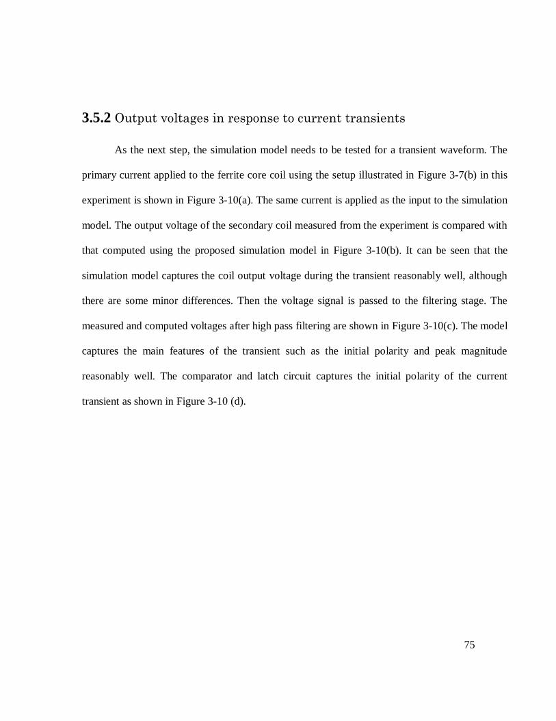
75
3.5.2 Output voltages in response to current transients
As the next step, the simulation model needs to be tested for a transient waveform. The
primary current applied to the ferrite core coil using the setup illustrated in Figure 3-7(b) in this
experiment is shown in Figure 3-10(a). The same current is applied as the input to the simulation
model. The output voltage of the secondary coil measured from the experiment is compared with
that computed using the proposed simulation model in Figure 3-10(b). It can be seen that the
simulation model captures the coil output voltage during the transient reasonably well, although
there are some minor differences. Then the voltage signal is passed to the filtering stage. The
measured and computed voltages after high pass filtering are shown in Figure 3-10(c). The model
captures the main features of the transient such as the initial polarity and peak magnitude
reasonably well. The comparator and latch circuit captures the initial polarity of the current
transient as shown in Figure 3-10 (d).
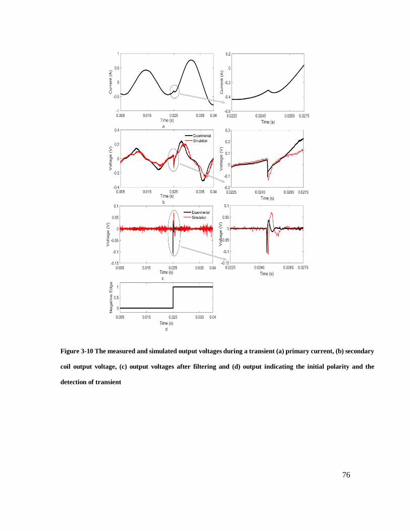
76
Figure 3-10 The measured and simulated output voltages during a transient (a) primary current, (b) secondary
coil output voltage, (c) output voltages after filtering and (d) output indicating the initial polarity and the
detection of transient
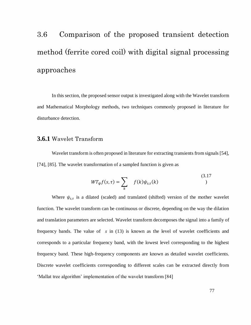
77
3.6 Comparison of the proposed transient detection
method (ferrite cored coil) with digital signal processing
approaches
In this section, the proposed sensor output is investigated along with the Wavelet transform
and Mathematical Morphology methods, two techniques commonly proposed in literature for
disturbance detection.
3.6.1 Wavelet Transform
Wavelet transform is often proposed in literature for extracting transients from signals [54],
[74], [85]. The wavelet transformation of a sampled function is given as
𝑊𝑇𝜓𝑓(𝑠, 𝜏) = ∑
𝑘
𝑓(𝑘)𝜓𝑠,𝜏(𝑘)
(3.17
)
Where 𝜓𝑠,𝜏 is a dilated (scaled) and translated (shifted) version of the mother wavelet
function. The wavelet transform can be continuous or discrete, depending on the way the dilation
and translation parameters are selected. Wavelet transform decomposes the signal into a family of
frequency bands. The value of 𝑠 in (13) is known as the level of wavelet coefficients and
corresponds to a particular frequency band, with the lowest level corresponding to the highest
frequency band. These high-frequency components are known as detailed wavelet coefficients.
Discrete wavelet coefficients corresponding to different scales can be extracted directly from
‘Mallat tree algorithm’ implementation of the wavelet transform [84]
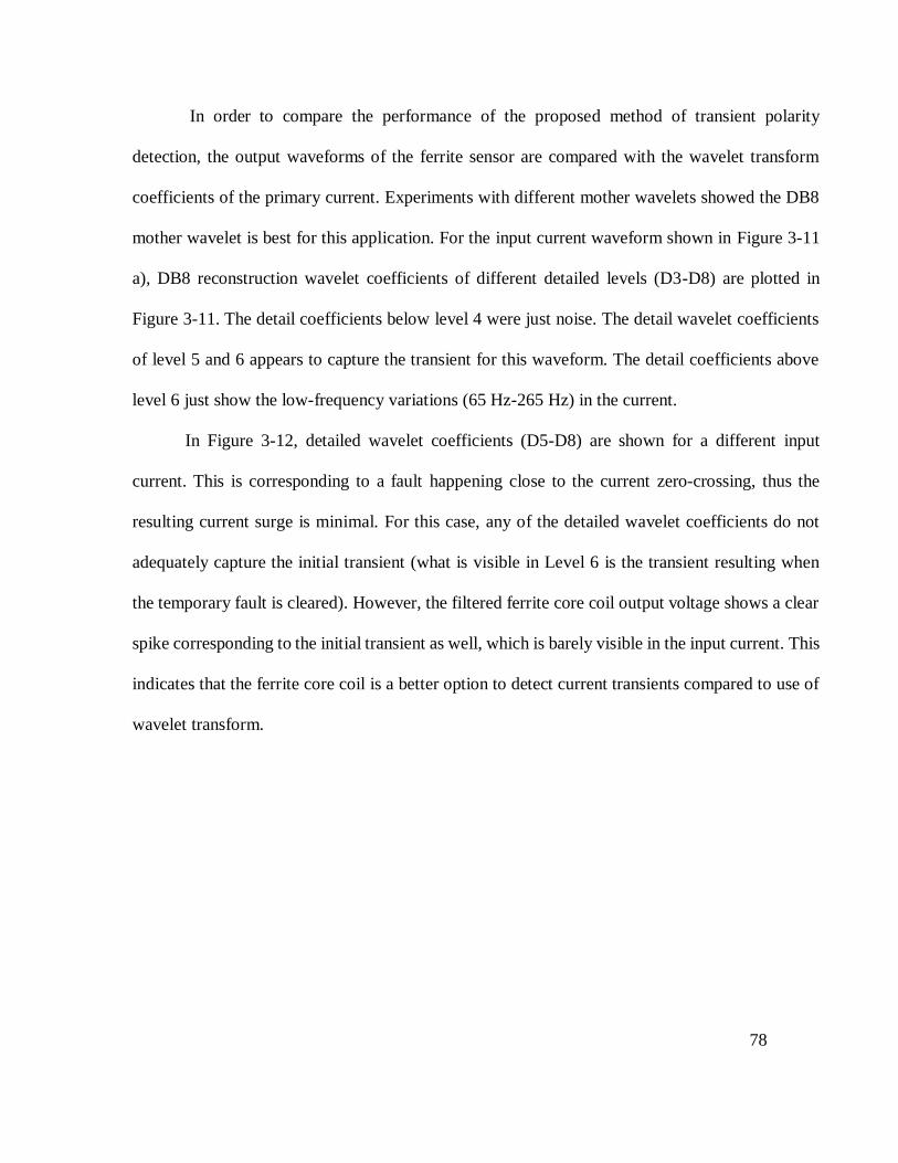
78
In order to compare the performance of the proposed method of transient polarity
detection, the output waveforms of the ferrite sensor are compared with the wavelet transform
coefficients of the primary current. Experiments with different mother wavelets showed the DB8
mother wavelet is best for this application. For the input current waveform shown in Figure 3-11
a), DB8 reconstruction wavelet coefficients of different detailed levels (D3-D8) are plotted in
Figure 3-11. The detail coefficients below level 4 were just noise. The detail wavelet coefficients
of level 5 and 6 appears to capture the transient for this waveform. The detail coefficients above
level 6 just show the low-frequency variations (65 Hz-265 Hz) in the current.
In Figure 3-12, detailed wavelet coefficients (D5-D8) are shown for a different input
current. This is corresponding to a fault happening close to the current zero-crossing, thus the
resulting current surge is minimal. For this case, any of the detailed wavelet coefficients do not
adequately capture the initial transient (what is visible in Level 6 is the transient resulting when
the temporary fault is cleared). However, the filtered ferrite core coil output voltage shows a clear
spike corresponding to the initial transient as well, which is barely visible in the input current. This
indicates that the ferrite core coil is a better option to detect current transients compared to use of
wavelet transform.

79
Figure 3-11 Detail wavelet coefficients of DB8 mother wavelet. (a) Input current (b) Filtered ferrite coil
output (c)-(g) detail wavelet coefficients of Levels 3-8
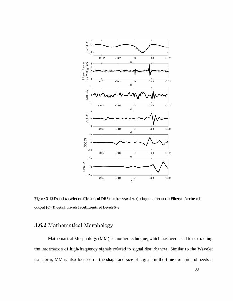
80
Figure 3-12 Detail wavelet coefficients of DB8 mother wavelet. (a) Input current (b) Filtered ferrite coil
output (c)-(f) detail wavelet coefficients of Levels 5-8
3.6.2 Mathematical Morphology
Mathematical Morphology (MM) is another technique, which has been used for extracting
the information of high-frequency signals related to signal disturbances. Similar to the Wavelet
transform, MM is also focused on the shape and size of signals in the time domain and needs a

81
smaller information window [50]. In MM, a Structural Element (SE) is used to extract the
necessary signal properties. MM consists of two basic operators called erosion and dilation. Based
on those primary operators, secondary operators such as opening and closing are defined [74].
The formulation of MM detailed in [74] is used to compare the effectiveness of the method
with proposed ferrite coil sensor. Assuming that 𝑓(𝑛) is the input signal as defined by a discrete
function with amplitudes 𝐷𝑓 = 0,1,2, … 𝑛 − 1 and 𝑔(𝑚)is an SE defined with amplitudes 𝐷𝑔 =
0,1,2, … 𝑚 − 1, then dilation of signal 𝑓 by 𝑔 is denoted by (𝑓 ⊕ 𝑔) and erosion of domain 𝑓 by
𝑔 is denoted by (𝑓 Ɵ 𝑔) and defined as follows:
𝑓𝑑𝑖𝑙 (𝑛) = (𝑓 ⊕ 𝑔) (𝑛) = 𝑚𝑎𝑥 𝑓(𝑛 + 𝑚) + 𝑔(𝑚) (3.18)
𝑓𝑒𝑟𝑜 (𝑛) = (𝑓Ɵ𝑔) (𝑛) = 𝑚𝑎𝑥 𝑓(𝑛 − 𝑚) − 𝑔(𝑚) (3.19)
By combining the above two operators, two other operators called opening and closing are
obtained. Opening operation of signal 𝑓 by 𝑔 is denoted by 𝑓 𝑔 and defined as:
𝑓𝑜𝑝𝑒𝑛(𝑛) = (𝑓 𝑔)(𝑛) = ((𝑓 ⊕ 𝑔)Ɵ𝑔)(𝑛) (3.20)
Also, the closing operation of signal f by g is denoted by 𝑓 • 𝑔 and defined as:
𝑓𝑐𝑙𝑜𝑠𝑒(𝑛) = (𝑓 • 𝑔)(𝑛) = ((𝑓Ɵ 𝑔) ⊕ 𝑔)(𝑛) (3.21)
Mathematical morphology function proposed by [50] is defined as follows,
𝑀𝑀𝐹3(𝑛) = (𝑓(𝑛) (𝑓 • 𝑔) (𝑛) + 𝑓 (𝑛) • (𝑓 𝑔)(𝑛))/2 (3.22)
𝑀𝑀𝐹3𝑑𝑖𝑙(𝑛) = (𝑀𝑀𝐹3 ⊕ 𝑔)(𝑛) (3.23)
𝑀𝑀𝐹3𝑒𝑟𝑜(𝑛) = (𝑀𝑀𝐹3 Ɵ 𝑔) (𝑛) (3.24)
𝑀𝑀𝐹𝑜𝑢𝑡𝑝𝑢𝑡(𝑛)
= 𝑀𝑀𝐹3𝑑𝑖𝑙(𝑛) − 𝑀𝑀𝐹3𝑒𝑟𝑜(𝑛) 𝑖𝑓 𝑀𝑀𝐹3𝑑𝑖𝑙(𝑛) − 𝑀𝑀𝐹3𝑑𝑖𝑙(𝑛 − 1) > 𝛿
𝑀𝑀𝐹3𝑒𝑟𝑜(𝑛) − 𝑀𝑀𝐹3𝑑𝑖𝑙(𝑛) 𝑖𝑓 𝑀𝑀𝐹3𝑒𝑟𝑜(𝑛) − 𝑀𝑀𝐹3𝑒𝑟𝑜(𝑛 − 1) > 𝛿
(3.25)
Reference [86] use the function corresponding to the difference between erosion (𝑒𝑟𝑜) and
dilation (𝑓𝑑𝑖𝑙) operators to identify the sudden changes of the signal while [74] uses the derived
operator (𝑀𝑀𝐹𝑜𝑢𝑡𝑝𝑢𝑡) from erosion (𝑒𝑟𝑜)and dilation (𝑓𝑑𝑖𝑙) operators. In [74], the use of MM is
82
demonstrated using mathematically synthesized signals, while, in [86] use of MM is demonstrated
with fault current waveforms obtained from simulations. In both the cases, visible transients were
present in the original input waveforms, and thus the corresponding outputs identified the edges.
Figure 3-13 shows the response of two suggested methods for the same experimental waveform.
The function defined in [74] produces two spikes, indicating the transient, but the function used in
[86] does not detect a clear transient, although it detects the changes in low-frequency components.
A comparison of ferrite coil response with the available signal processing methods shows
the superiority of the proposed transient sensor compared to those methods. Although wavelet
transform and MM are potent tools for signal processing, their performance may be limited by the
signal noise and analog to digital conversion precision.
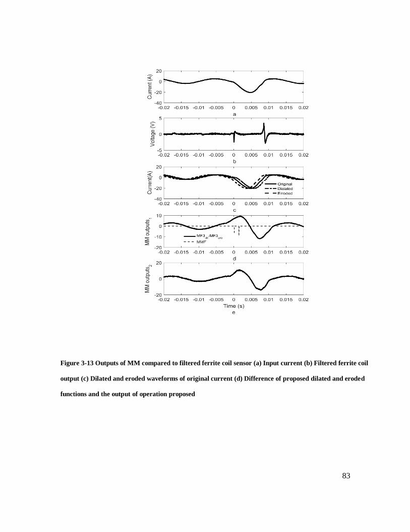
83
Figure 3-13 Outputs of MM compared to filtered ferrite coil sensor (a) Input current (b) Filtered ferrite coil
output (c) Dilated and eroded waveforms of original current (d) Difference of proposed dilated and eroded
functions and the output of operation proposed

84
3.7 Summary
In this chapter, the proposed ferrite core coil sensor performance is compared with other
potential current sensors for transient detection applications. Then a sensor system to detect initial
current transient polarity is proposed. Ferrite core coil was the central part of the sensor system.
The development of a mathematical model of the ferrite core coil to be used in an EMT type
simulation programs is presented. A method to incorporate dynamic behavior of core
characteristics to the mathematical model is proposed and validated with laboratory experiments.
Finally, the experimental output of the ferrite core coil is compared with two signal-processing
methods used in detecting transient edges in the literature.

85
Chapter 4 Chapter 4
A hybrid protection scheme for active
distribution networks
The integration of DER poses many challenges to traditional distribution protection as
detailed in Chapter 2. Since DER connected to the distribution networks generally have low or
negligible inertia, the implementation of fast protection is essential to maintain the stability of
DER connected to healthy parts of the distribution network. A new hybrid protection strategy is
proposed in this thesis combining the features of both traditional protection methods and transient
based protection methods to provide sensitive, reliable, and fast protection solutions for active
distribution networks and microgrids. The content of this chapter is based on the original work
published in;
A. Pathirana, A. Rajapakse, and N. Perera, “Development of a hybrid protection scheme
for active distribution systems using polarities of current transients,” Electric Power Systems
Research, vol. 152, pp. 377–389, Nov. 2017 [47], and
N. Pathirana, A. D. Rajapakse, “Enhancing the transient stability of distributed generators
with adaptive time-overcurrent protection augmented with transient based unit protection”,
International Conference on Power Systems Transients (IPST), Cavtat, Croatia, pp. 15-18, Jun.
2015 [87].

86
4.1 Introduction
Different issues related to the protection of active distribution systems with a mix of
synchronous, induction, and inverter-based generators were discussed in detail in Chapter 2. A
variety of solutions that have been proposed in the literature to address the aforementioned
challenges associated with the active distribution systems were also presented in Chapter 2, with
a brief discussion of their merits and limitations.
This chapter introduces a hybrid protection scheme, where the operation of the
conventional protection schemes is accelerated while improving the selectivity and sensitivity by
utilizing a transient based technique to discriminate the faults. In the proposed method, ferrite core
coil sensors proposed in Chapter 3 are used to detect and identify the polarities of fault current
transients. Although the use of ferrite coils for transient current measurements is fairly established
[10], this research work investigates its application in a novel fashion for detecting faults and
determining the faulted zone by comparing the transient polarities. The security of protection is
enhanced by using traditional protection schemes to supervise the decision of transient protection.
The performance of the proposed method was initially evaluated using three distribution systems
simulated in an electromagnetic transient (EMT) type simulation program. The third network
demonstrates the application of the proposed method for a more extensive benchmark distribution
system.

87
4.2 Faulty section identification using current
transients
The proposed protection scheme determines whether a fault is inside or outside the
protected zone by comparing the polarities of the current transients extracted at the boundary of
the protected zone. Although this concept appears similar to the line current differential protection,
the actual measured signals are not exchanged between the two ends. Only the polarities of the
initial transients on each of the phase currents are sent to the other end via a telecommunication
link. The measurements require no time synchronization. Thus the bandwidth requirement of the
telecommunication is minimal. Since no time synchronization is necessary, the scheme can be
implemented with a low hardware cost. The polarities are compared on a phase-by-phase basis for
internal and external fault identification. Figure 4-1 and Figure 4-2 graphically illustrate the
possible polarities of the current transients for an external fault and an internal fault respectively.
If the polarity of current measurements is such that currents entering the protected zone are
measured as positive at both ends, opposite polarities in current transients indicate that the fault is
located outside the protected zone whereas the same polarities indicate that the fault is located
inside the protected zone. Here, the external and internal refers to the fault location relative to the
zone between the two measurement locations.
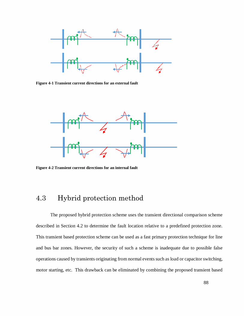
88
Figure 4-1 Transient current directions for an external fault
Figure 4-2 Transient current directions for an internal fault
4.3 Hybrid protection method
The proposed hybrid protection scheme uses the transient directional comparison scheme
described in Section 4.2 to determine the fault location relative to a predefined protection zone.
This transient based protection scheme can be used as a fast primary protection technique for line
and bus bar zones. However, the security of such a scheme is inadequate due to possible false
operations caused by transients originating from normal events such as load or capacitor switching,
motor starting, etc. This drawback can be eliminated by combining the proposed transient based

89
technique with a conventional protection scheme as shown in Figure 4-3, where conventional
protection is used to confirm the existence of a fault. In the hybrid protection, actual trip signals
are always supervised by conventional protection; thus the possibility of false tripping due to non-
fault related transients is avoided. Since the fault discrimination is achieved using transient based
protection, conventional protection can be set more sensitively and without excessive time delays,
speeding up the overall operation (fault detection and isolation).
Two ways of realizing the hybrid protection scheme is discussed in the following sections.
First, the proposed hybrid protection method is implemented in conjunction with conventional
overcurrent protection, typically used in distribution system protection. Next, the hybrid protection
approach is applied in conjunction with conventional distance protection to improve the operation
of a Permissive Overreach Transfer Trip (POTT) scheme.

90
Figure 4-3 Flow diagram showing the operation of the proposed hybrid protection method
a) Hybrid overcurrent protection scheme
The main protection philosophy used in the distribution level applications is based on the
coordinated directional or non-directional time-overcurrent relays and instantaneous overcurrent
relays. The time-overcurrent relays are coordinated with each other by adjusting the pickup current
and time dial settings (TDS) based on the fault levels at each bus. A discrimination margin of 0.2-
0.4 s is maintained between two adjacent overcurrent relays.
In the hybrid protection scheme, instantaneous overcurrent function or a fast curve of the
time-overcurrent function is used to supervise the transient based scheme: if a fault is identified as
Read ferrite coil voltages
Start
Transient detected?
Compare polarities of the transients
Internal fault?
Yes
Conventional Protection
Determine the polarity of the
transient
Trip
Input Currents/Voltages Polarity from the
remote end
Transient Based
Protection
No
YesNo
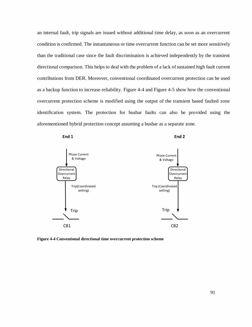
91
an internal fault, trip signals are issued without additional time delay, as soon as an overcurrent
condition is confirmed. The instantaneous or time overcurrent function can be set more sensitively
than the traditional case since the fault discrimination is achieved independently by the transient
directional comparison. This helps to deal with the problem of a lack of sustained high fault current
contributions from DER. Moreover, conventional coordinated overcurrent protection can be used
as a backup function to increase reliability. Figure 4-4 and Figure 4-5 show how the conventional
overcurrent protection scheme is modified using the output of the transient based faulted zone
identification system. The protection for busbar faults can also be provided using the
aforementioned hybrid protection concept assuming a busbar as a separate zone.
Figure 4-4 Conventional directional time overcurrent protection scheme
Phase Current & Voltage
Trip (Coordinated setting)
Trip Trip
Phase Current & Voltage
End 2End 1
Directional Overcurrent
Relay
Directional Overcurrent
Relay
CB1 CB2
Trip(Coordinated setting)

92
Figure 4-5 Hybrid overcurrent protection scheme
b) Hybrid distance protection scheme
Although the primary focus of this thesis is distribution systems, the proposed hybrid
protection can be applied to transmission protection, especially in conjunction with distance
protection. This possibility is discussed in this section, as distance protection is sometimes
proposed for the protection of medium voltage distribution feeders with DER. The permissive
overreach transfer trip (POTT) scheme commonly used in transmission line protection relies on
the Zone-2 pickup signal receiving from the remote end. The weak infeed support is provided to
accommodate the lack of significant fault current contribution from the DER for faults far from
the grid side. This typically is achieved by echoing back the received signal after a short delay, as
shown in the detailed protection logic of the POTT scheme shown in Figure 4-6.
Trip(Fast
Setting)
Phase Current & Voltage
Trip(Coordinated
setting)
Trip(Fast Setting)
Trip Trip
Phase Current & Voltage
End 2
Internal Fault
End 1
Internal Fault
Directional Overcurrent
Relay
Directional Overcurrent
Relay
CB1 CB2
Trip (Coordinated
setting)
Transient Protection
Unit
Transient Protection
Unit
Com.Delay
Ferrite coil voltages
Ferrite coil voltages

93
During a fault, Zone-2 pickup goes high without any added delays. That signal is sent to
the other end of the protected line segment and relayed back after a delay. This is to ensure the
operation of the relay in case of a weak infeed. In addition to that, pickup signal from the other
end of the protected line segment can trigger the trip operation as well.
Figure 4-6 Conventional distance protection with POTT with weak infeed echo feature
In the proposed hybrid protection scheme, the trip signal from the transient based
protection is supervised by the Zone-2 pickup signals, as shown in Figure 4-7. As the hybrid
protection is very fast even when a typical communication delay is considered, this scheme enables
tripping breakers as soon as the Zone-2 pickup signal verifies the fault. The original POTT scheme
stays intact, providing backup for the faster tripping scheme. For this modified protection scheme,
two additional communication channels are required to exchange transient polarities.
Zon
e 2
Zon
e 2
Zon
e 2
Pick
up
TripTrip
Current & Voltage
End 2
Zon
e 1
Current & Voltage
End 1
Zon
e 2
Pic
k u
p
Distance Relay
Distance Relay
CB1 CB2
Com.Delay
Com.Delay
Zon
e 1
POTT with weak infeed
DelayPOTT
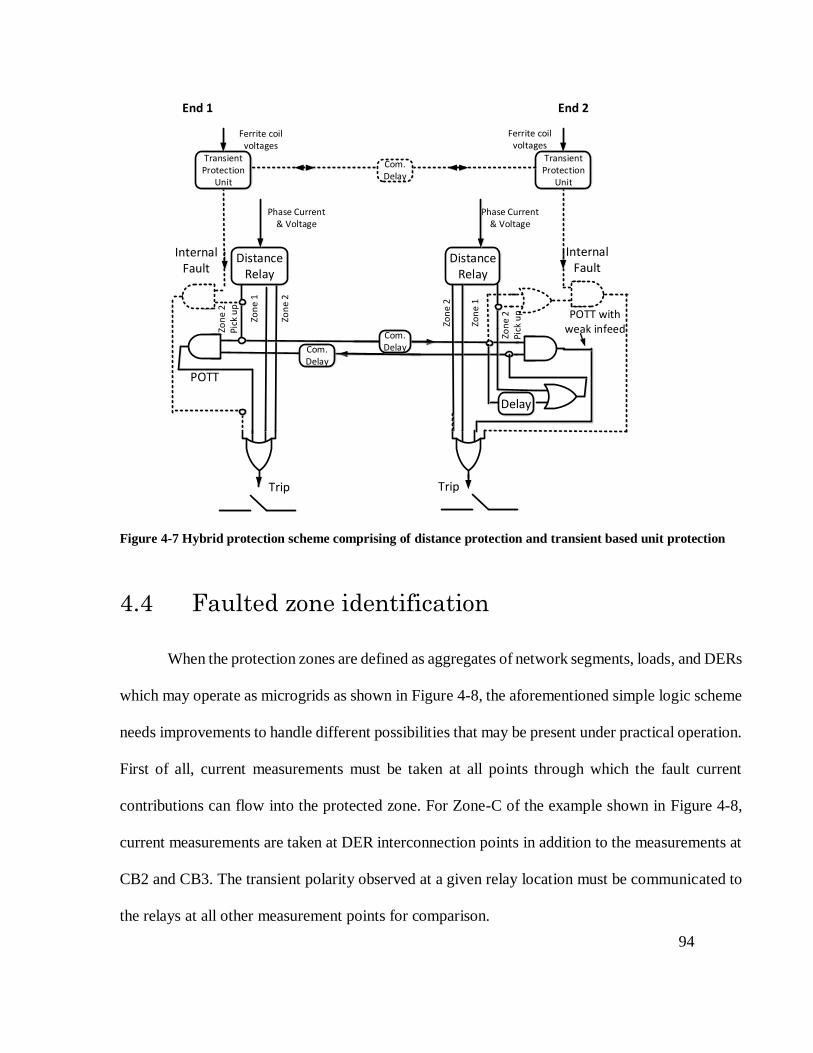
94
Figure 4-7 Hybrid protection scheme comprising of distance protection and transient based unit protection
4.4 Faulted zone identification
When the protection zones are defined as aggregates of network segments, loads, and DERs
which may operate as microgrids as shown in Figure 4-8, the aforementioned simple logic scheme
needs improvements to handle different possibilities that may be present under practical operation.
First of all, current measurements must be taken at all points through which the fault current
contributions can flow into the protected zone. For Zone-C of the example shown in Figure 4-8,
current measurements are taken at DER interconnection points in addition to the measurements at
CB2 and CB3. The transient polarity observed at a given relay location must be communicated to
the relays at all other measurement points for comparison.
Internal Fault
Zon
e 2
Zon
e 2
Zon
e 2
Pick
up
Trip Trip
Phase Current & Voltage
End 2
Zon
e 1
Phase Current & Voltage
End 1
Zon
e 2
Pick
up
Distance Relay
Distance Relay
Com.Delay
Com.Delay
Zon
e 1
Delay
POTT
POTT with weak infeed
Internal Fault
Transient Protection
Unit
Transient Protection
Unit
Com.Delay
Ferrite coil voltages
Ferrite coil voltages

95
Also the possibility of having one or more breakers at the zone boundary open under pre-
fault conditions must be considered: network segments or DERs could be taken out of operation
for repair and maintenance or due to previous faults. There is no current flow through an open
breaker and the current transient polarity signal corresponding open breaker location should be
omitted from the polarity comparison logic used for fault discrimination. In order to avoid
generating spurious polarity signals, polarity signals can be supervised using a breaker status signal
(or an undercurrent element), as shown in Figure 4-9. Similarly, when the source feeding a faulted
zone is weak (for example infeed from a DER), the transients generated during a remote fault or a
non-fault related event could become too small to generate a valid polarity signal for the event. In
such a scenario, no polarity signal would be sent from the relays that sense too weak transients.
The logic for faulted zone identification must be enhanced to deal with these practical
possibilities. Thus when some of the relays on the boundary of a zone send neither positive polarity
signal nor negative polarity signal due to open breakers or weak transients, a relay that observe a
transient has to make a decision considering the polarity signals that are available. This situation
is resolved as follows:
If there are at least two locations that sensed opposite polarity transients, declare the fault as
external.
Otherwise, if at least two of the polarity signals are positive and none of the polarity signals
are negative, or at least two of the polarity signals are negative and none of the polarity signals
are positive, declare an internal fault.
If neither of the above conditions are met, including when only one valid polarity signal is
available, the fault location (internal/external) is undetermined and a default decision
(typically external fault) is taken. This will not lead to any immediate false tripping during

96
non-fault events due to supervision by the conventional protection element at the relay
location.
For example, consider CB3 in Figure 4-8 was previously open, and for a fault in Zone-C,
it will be declared as an internal fault by the transient polarities sensed by the relay at CB2, which
will sense a strong transient due to grid infeed, and the relays at DER-3 and DER-4.
Figure 4-8 Case where a beaker opens and divides the network into two segments
Figure 4-9 Supervising polarity signal with breaker status
CB2
Zone-C
CB3 CB4
Zone-D
fault
Zone-B
CB1
To Other Zone Boundary
+
To Other Zone Boundary
+ve Transient Polarity
-ve Transient Polarity
Brk Close
Px
Nx
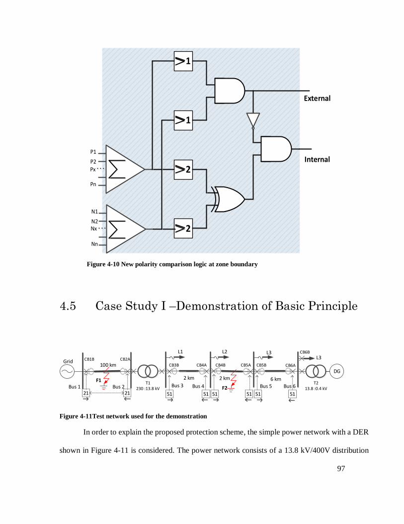
97
Figure 4-10 New polarity comparison logic at zone boundary
4.5 Case Study I –Demonstration of Basic Principle
Figure 4-11Test network used for the demonstration
In order to explain the proposed protection scheme, the simple power network with a DER
shown in Figure 4-11 is considered. The power network consists of a 13.8 kV/400V distribution
P1
P2
Pn
2
N1
N2
Nn
2
Internal
1
1
External
Px
Nx
Grid
Bus 1
CB1B
Bus 2 Bus 3T1
230 :13.8 kV
CB2A
100 km
Bus 4 Bus 5 Bus 6
CB3B CB4A CB4B CB5A CB6A
CB6B
CB5B
2 km 6 km
L1 L2
DG
T213.8 :0.4 kV
2 km
F2
F1
L3L3
515121 21 51515151
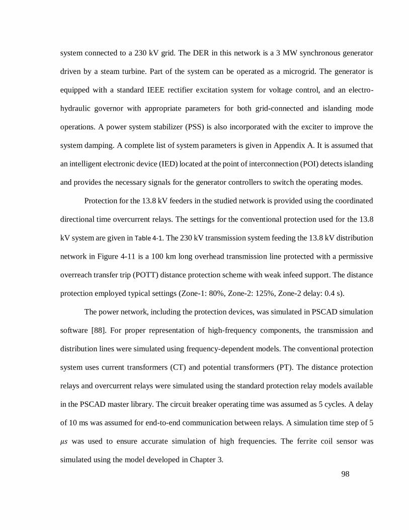
98
system connected to a 230 kV grid. The DER in this network is a 3 MW synchronous generator
driven by a steam turbine. Part of the system can be operated as a microgrid. The generator is
equipped with a standard IEEE rectifier excitation system for voltage control, and an electro-
hydraulic governor with appropriate parameters for both grid-connected and islanding mode
operations. A power system stabilizer (PSS) is also incorporated with the exciter to improve the
system damping. A complete list of system parameters is given in Appendix A. It is assumed that
an intelligent electronic device (IED) located at the point of interconnection (POI) detects islanding
and provides the necessary signals for the generator controllers to switch the operating modes.
Protection for the 13.8 kV feeders in the studied network is provided using the coordinated
directional time overcurrent relays. The settings for the conventional protection used for the 13.8
kV system are given in Table 4-1. The 230 kV transmission system feeding the 13.8 kV distribution
network in Figure 4-11 is a 100 km long overhead transmission line protected with a permissive
overreach transfer trip (POTT) distance protection scheme with weak infeed support. The distance
protection employed typical settings (Zone-1: 80%, Zone-2: 125%, Zone-2 delay: 0.4 s).
The power network, including the protection devices, was simulated in PSCAD simulation
software [88]. For proper representation of high-frequency components, the transmission and
distribution lines were simulated using frequency-dependent models. The conventional protection
system uses current transformers (CT) and potential transformers (PT). The distance protection
relays and overcurrent relays were simulated using the standard protection relay models available
in the PSCAD master library. The circuit breaker operating time was assumed as 5 cycles. A delay
of 10 ms was assumed for end-to-end communication between relays. A simulation time step of 5
𝜇𝑠 was used to ensure accurate simulation of high frequencies. The ferrite coil sensor was
simulated using the model developed in Chapter 3.

99
Table 4-1 Conventional over currents relay settings of the network
Relay CT Ratio Pickup Current (A)
(Secondary)
TDS
CB6B 40:5 3.6 0.05
CB5B 40:5 3.6 0.16
CB4B 100:5 4.6 0.20
CB3B 125:5 4.7 0.28
The hybrid protection scheme is comprised of transient based protection and traditional
protection mechanism. The central part of the transient based protection is the identification of
initial current polarities of high-frequency current transients. Following section details that
process.
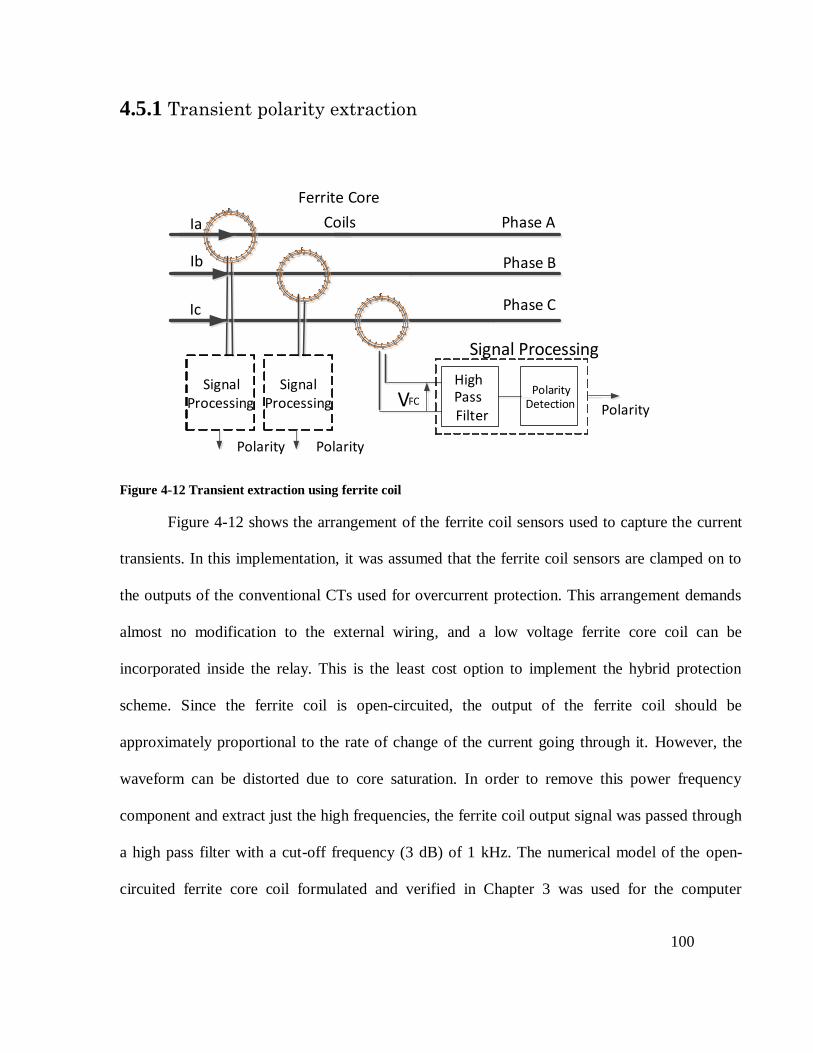
100
4.5.1 Transient polarity extraction
Figure 4-12 Transient extraction using ferrite coil
Figure 4-12 shows the arrangement of the ferrite coil sensors used to capture the current
transients. In this implementation, it was assumed that the ferrite coil sensors are clamped on to
the outputs of the conventional CTs used for overcurrent protection. This arrangement demands
almost no modification to the external wiring, and a low voltage ferrite core coil can be
incorporated inside the relay. This is the least cost option to implement the hybrid protection
scheme. Since the ferrite coil is open-circuited, the output of the ferrite coil should be
approximately proportional to the rate of change of the current going through it. However, the
waveform can be distorted due to core saturation. In order to remove this power frequency
component and extract just the high frequencies, the ferrite coil output signal was passed through
a high pass filter with a cut-off frequency (3 dB) of 1 kHz. The numerical model of the open-
circuited ferrite core coil formulated and verified in Chapter 3 was used for the computer
Ferrite Core
Coils Phase A
Phase B
Phase C
Ia
Ib
Ic
VFC
Signal Processing
High Pass Filter
Polarity Detection Polarity
Polarity
Signal Processing
Polarity
Signal Processing
101
simulations. The initial polarities of the high pass filtered transient signals were used to identify
the faulted network segments.
For the power network shown in Figure 4-11, the ferrite coils sensors associated with CB1B
and CB2A are used with the protection for 230 kV transmission line segment between Bus-1 and
Bus-2 and those associated with CB4B and CB5A are used with the protection for distribution line
segment between Bus-4 and Bus-5. Thus for protection of the transmission line segment between
Bus-1 and Bus-2, fault F1 is considered to be an internal fault whereas, fault F2 is considered as
an external fault. Figure 4-13 shows the fault currents and ferrite coil voltages measured at CB1B
and CB2A for the internal fault F1 and the external fault F2 respectively. The first column of
Figure 4-13 shows voltage and current waveforms after the fault F1, while the second column
shows the resulting waveforms after the fault F2. The first row of waveforms show the line currents
after the fault. The second row of waveforms show the resulting ferrite coil voltages. Then the
ferrite coil voltages are filtered, and the resulting waveforms are used to determine the polarity of
the transients. As can be seen from the plots that the current transient polarities extracted at two
ends are the same for the internal fault, and they are opposite for the external fault.
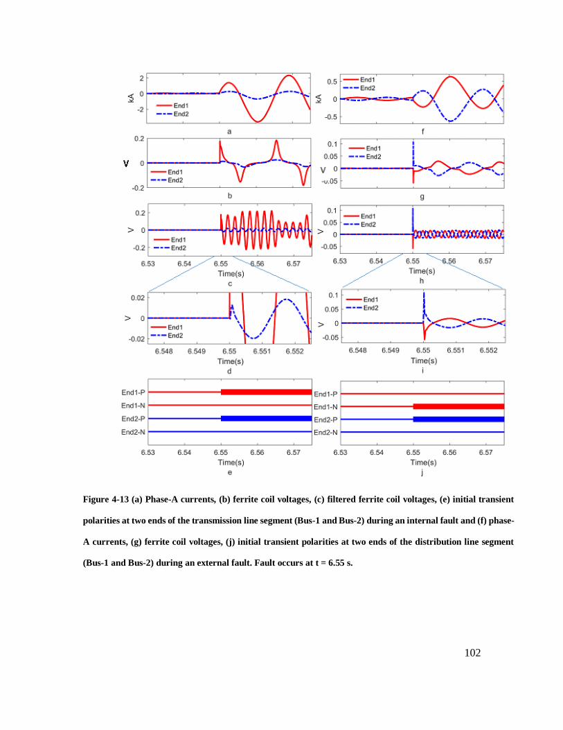
102
Figure 4-13 (a) Phase-A currents, (b) ferrite coil voltages, (c) filtered ferrite coil voltages, (e) initial transient
polarities at two ends of the transmission line segment (Bus-1 and Bus-2) during an internal fault and (f) phase-
A currents, (g) ferrite coil voltages, (j) initial transient polarities at two ends of the distribution line segment
(Bus-1 and Bus-2) during an external fault. Fault occurs at t = 6.55 s.
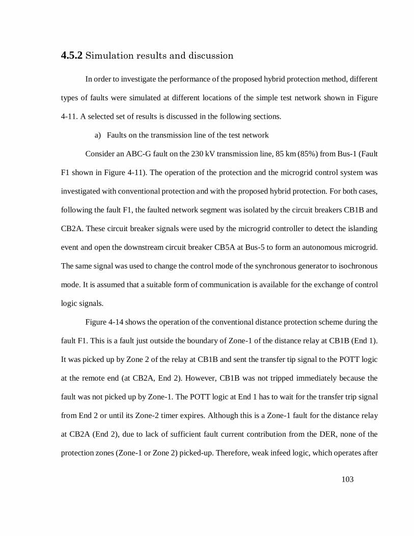
103
4.5.2 Simulation results and discussion
In order to investigate the performance of the proposed hybrid protection method, different
types of faults were simulated at different locations of the simple test network shown in Figure
4-11. A selected set of results is discussed in the following sections.
a) Faults on the transmission line of the test network
Consider an ABC-G fault on the 230 kV transmission line, 85 km (85%) from Bus-1 (Fault
F1 shown in Figure 4-11). The operation of the protection and the microgrid control system was
investigated with conventional protection and with the proposed hybrid protection. For both cases,
following the fault F1, the faulted network segment was isolated by the circuit breakers CB1B and
CB2A. These circuit breaker signals were used by the microgrid controller to detect the islanding
event and open the downstream circuit breaker CB5A at Bus-5 to form an autonomous microgrid.
The same signal was used to change the control mode of the synchronous generator to isochronous
mode. It is assumed that a suitable form of communication is available for the exchange of control
logic signals.
Figure 4-14 shows the operation of the conventional distance protection scheme during the
fault F1. This is a fault just outside the boundary of Zone-1 of the distance relay at CB1B (End 1).
It was picked up by Zone 2 of the relay at CB1B and sent the transfer tip signal to the POTT logic
at the remote end (at CB2A, End 2). However, CB1B was not tripped immediately because the
fault was not picked up by Zone-1. The POTT logic at End 1 has to wait for the transfer trip signal
from End 2 or until its Zone-2 timer expires. Although this is a Zone-1 fault for the distance relay
at CB2A (End 2), due to lack of sufficient fault current contribution from the DER, none of the
protection zones (Zone-1 or Zone 2) picked-up. Therefore, weak infeed logic, which operates after
104
a 0.3 s delay, came into effect. The POTT scheme had to wait for the echo back signal to generate
trip signals at both ends of the transmission line. This resulted in around 350 ms trip time
(excluding the circuit breaker operating time, communication delay was assumed as 10 ms).
Figure 4-14 Operation of the protection during fault F1 with conventional protection a) line current End-1, b)
line current End-2 ,c) CT secondary current End-1 ,d) CT secondary current End-2 ,e) ferrite coil voltage End-
1 ,f) ferrite coil voltage End-2 ,g) & i) filtered ferrite coil voltage End-1 ,h) & j) filtered ferrite coil voltage End-
2 ,k) internal fault, Zone2- Alarm, Zone1, Zone2, Trip End-1 ,l) internal fault, Zone2- alarm, Zone1, Zone2,
TripEnd-2

105
Figure 4-15 Operation of the protection during fault F1 with hybrid protection operation of the protection
during fault F1 with conventional protection ,a) line current End-1 ,b) line current End-2 ,c) CT secondary
current End-1 ,d) CT secondary current End-2 ,e) ferrite coil voltage End-1 ,f) ferrite coil voltage End-2 ,g &
i) filtered ferrite coil voltage End-1 ,h) & j) filtered ferrite coil voltage End-2 ,k) internal fault, Zone2- Alarm,
Zone1, Zone2, Trip End-1 ,l) internal fault, Zone2- alarm, Zone1, Zone2, TripEnd-2
Figure 4-15 shows the operation of the hybrid protection scheme for the same fault (F1).
The transient based unit protection detected the fault F1 and identified it as an internal fault within
10 ms after the fault at both ends. Thus a trip signal was issued to CB1B as soon as the fault was
picked up by Zone-2 of the distance relay at End 1. By advancing the operation of the POTT
106
scheme, an overall trip time of around 22 ms could be achieved at End 1 (excluding the circuit
breaker operating time).
During the faults, the active and reactive power supplied to the loads from the grid is
disrupted and the synchronous generator starts to accelerate, as its electrical power output is
restricted due to low terminal voltages during the fault. If the fault is not cleared rapidly, the
frequency and voltage of the generator tends to deviate far from the acceptable values specified by
the interconnecting standards. Figure 4-16 compares the voltage and frequency responses of the
formed microgrid system followed by the operation of the conventional protection scheme and the
hybrid protection scheme. As it can be observed from Figure 4-16, the fast response of the hybrid
protection has helped to maintain the voltage and frequency profiles closer to the nominal values,
demonstrating improved system performances compared to conventional protection.

107
Figure 4-16 Voltage and frequency profiles of the synchronous DG during fault F1
In order to investigate the robustness of the proposed protection method, the fault F1 was
simulated with different types of faults such as AG, BC, BCG, and ABC. Table 4-2 summarizes the
speed comparison of the two protection schemes. According to the results, the hybrid protection
scheme demonstrates a faster response compared to the conventional protection for all simulated
faults on the transmission line.
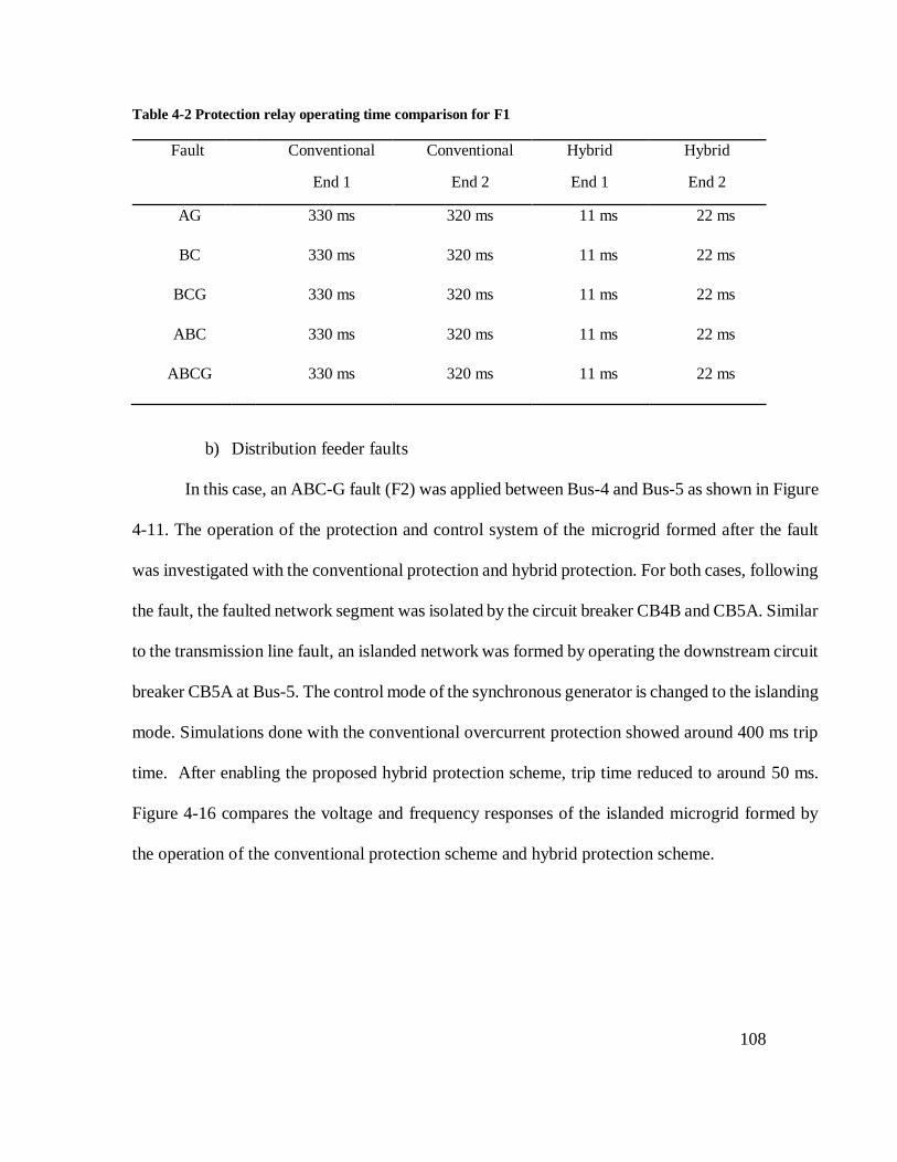
108
Table 4-2 Protection relay operating time comparison for F1
Fault Conventional
End 1
Conventional
End 2
Hybrid
End 1
Hybrid
End 2
AG 330 ms 320 ms 11 ms 22 ms
BC 330 ms 320 ms 11 ms 22 ms
BCG 330 ms 320 ms 11 ms 22 ms
ABC 330 ms 320 ms 11 ms 22 ms
ABCG 330 ms 320 ms 11 ms 22 ms
b) Distribution feeder faults
In this case, an ABC-G fault (F2) was applied between Bus-4 and Bus-5 as shown in Figure
4-11. The operation of the protection and control system of the microgrid formed after the fault
was investigated with the conventional protection and hybrid protection. For both cases, following
the fault, the faulted network segment was isolated by the circuit breaker CB4B and CB5A. Similar
to the transmission line fault, an islanded network was formed by operating the downstream circuit
breaker CB5A at Bus-5. The control mode of the synchronous generator is changed to the islanding
mode. Simulations done with the conventional overcurrent protection showed around 400 ms trip
time. After enabling the proposed hybrid protection scheme, trip time reduced to around 50 ms.
Figure 4-16 compares the voltage and frequency responses of the islanded microgrid formed by
the operation of the conventional protection scheme and hybrid protection scheme.

109
Figure 4-17 Operation of the protection during fault F2 without hybrid protection a),b) Phase A currents at
each end c),d) Phase A ferrite coil voltages e),f) Filtered phase A ferrite coil voltages (Zoomed) g),h)Fault time
and overcurrent relay operation time

110
Figure 4-18 Operation of the protection during fault F2 with hybrid protection a),b) Phase A currents at each
end c),d) Phase A ferrite coil voltages e),f) ) Filtered phase A ferrite coil voltages (Zoomed) g),h) Fault time
and overcurrent relay operation time
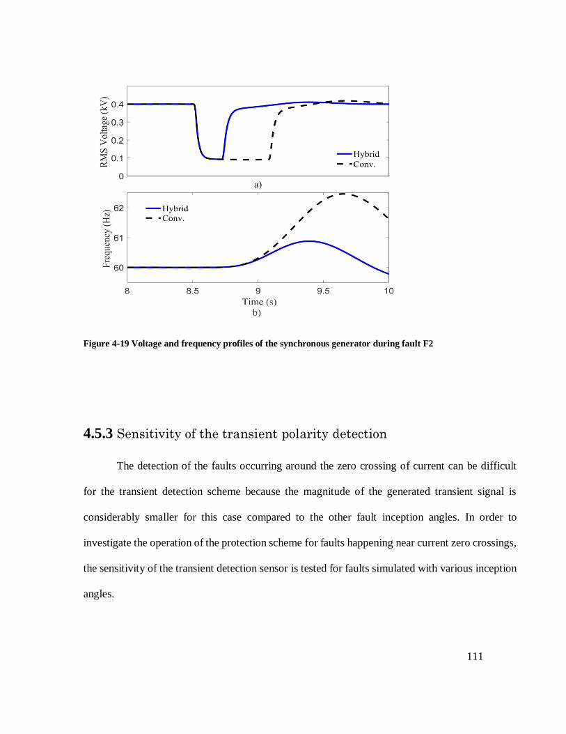
111
Figure 4-19 Voltage and frequency profiles of the synchronous generator during fault F2
4.5.3 Sensitivity of the transient polarity detection
The detection of the faults occurring around the zero crossing of current can be difficult
for the transient detection scheme because the magnitude of the generated transient signal is
considerably smaller for this case compared to the other fault inception angles. In order to
investigate the operation of the protection scheme for faults happening near current zero crossings,
the sensitivity of the transient detection sensor is tested for faults simulated with various inception
angles.

112
Test network used for Case study-I is used to analyze the sensitivity of the transient polarity
detection to the fault inception angle. Three-phase faults with various fault inception angles are
applied to the line segment between Bus 1 and Bus 2. Resulting CT currents are shown in Figure
4-20. The absence of sharp change in the current signals are clearly visible when the fault inception
angle approaches zero.
The resulting ferrite coil voltages are shown in Figure 4-21. For all the tested fault inception angles
less than 4°, output voltages of the ferrite coils are greater than 0.2 volts with clearly visible sharp
change, which is necessary for the transient based polarity detection scheme. When the fault
inception angles are near 90°, output voltages of the ferrite core coils can reach up to 100 volts.
For the fault inception angles below 4°, the output of the transient polarity detection scheme can
be less reliable. The proposed transient polarity detection method is also not completely immune
to this common issue that hinders most of the transient based protection algorithms,

113
Figure 4-20 CT secondary currents at Bus 1 and Bus 2, after solid three phase faults at different fault inception
angles. End 1- left column, End 2 – right column

114
Figure 4-21 Ferrite coil voltages at Bus 1 and Bus 2, after solid three phase faults at different fault inception
angles. End 1- left column, End 2 – right column

115
4.5.4 Effect of inverter interfaced DER on transient polarity detection
To investigate the response of the polarity detection sensor to the inverter interface DER,
the synchronous generator of Case study-I is replaced with an inverter based energy source. After
replacing the synchronous generator, three-phase solid faults were applied in the feeder between
Bus 4 and Bus 5. The CT secondary current responses of the faulted line segment is shown in
Figure 4-22. Figure 4-22 indicates that there is no significant fault current contribution from the
inverter towards the fault while the fault current contribution from the grid side is similar to the
case with the synchronous generator. Note that fault current from the inverter side drops below the
pre-fault load current in the line, which is actually flowing from the grid towards the load
connected at Bus 5. The current after the fault is the contribution of the inverter.
The resulting ferrite coil voltages are shown in Figure 4-23 Ferrite coil voltages at Bus 4
and Bus 5, after solid three- phase faults at two different fault inception angles. End 1- left column,
End 2 – right column. (After the synchronous generator is replaced with an inverter interfaced energy
source)Although the steady state fault current from the inverter is highly limited, the transient
signals are still present. The output voltage magnitudes of the ferrite coils are in the similar range
compared to the case with synchronous generators. This indicates that the inverter interfaced DER
are not a challenge for the transient polarity detection scheme. However, it could be a challenge
for the conventional protection in the hybrid scheme.

116
Figure 4-22 CT secondary currents at Bus 4 and Bus 5, after a solid three-phase faults at two different fault
inception angles. End 1- left column, End 2 – right column. (After synchronous generator is replaced by an
inverter interfaced energy source)
Figure 4-23 Ferrite coil voltages at Bus 4 and Bus 5, after solid three- phase faults at two different fault inception
angles. End 1- left column, End 2 – right column. (After the synchronous generator is replaced with an inverter
interfaced energy source)

117
4.6 Case Study II - Solving potential DER stability
problems with the hybrid protection approach
The primary intention of this part of the study is to use the proposed hybrid protection
methodology to maintain the stable operation of synchronous generators (DER units) after a fault
which would otherwise trip the DER unit.
In order to demonstrate that point, a simple test network is used for the study. The test
network shown in Figure 4-24 is used to demonstrate the problem and the solution provided. This
network contains two 5.5 MVA diesel generators connected to a 13.2 kV distribution system. The
DER units are designed to operate as a microgrid in case of loss of mains supply and provide power
to critical loads connected to Bus 3 and Bus 2. Although the two generators are of the same
capacity, DER2 has a higher inertia. The loads connected to Bus 2 and Bus 3 draw 9 MW of active
power and 2 Mvar of reactive power. A part of the loads amounting to 2 MW is considered to be
non-critical and shed in the event of losing the grid supply.
Under normal mode of operation in parallel with the grid, both the DER units are operated
as constant power generators. In case of loss of grid supply, the control systems of the two diesel
generators are changed. DER2 is switched to isochronous operation to control the frequency in the
isolated microgrid.
It is assumed that the overcurrent protection scheme of the network has been designed
prior to the interconnection of DER units, as such, the protection settings have been determined
without considering the two generators. Since the synchronous generators can provide sustained
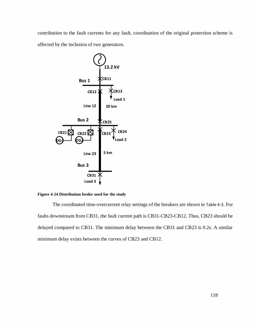
118
contribution to the fault currents for any fault, coordination of the original protection scheme is
affected by the inclusion of two generators.
Figure 4-24 Distribution feeder used for the study
The coordinated time-overcurrent relay settings of the breakers are shown in Table 4-3. For
faults downstream from CB31, the fault current path is CB31-CB23-CB12. Thus, CB23 should be
delayed compared to CB31. The minimum delay between the CB31 and CB23 is 0.2s. A similar
minimum delay exists between the curves of CB23 and CB12.
DG2
13.2 kV
Bus 1
Bus 2
Bus 3
CB22 CB23
CB13
20 km
5 km
Load 1
Load 3
DG1
CB21
CB11
CB12
CB25
CB31
Load 2
CB24
Line 12
Line 23

119
Table 4-3 Time overcurrent relay settings
Relay CT Ratio Pickup Current (A)
(Secondary)
TDS
CB31 150:5 4.16 0.05
CB23 300:5 4.16 0.09
CB12 500:5 3.75 0.13
4.6.1 Identified stability issues
a) Case I: Prolonged fault on Line 12
For a fault between Bus1 and Bus 2 in the network shown in Figure 4-24, the expected
response is to remove Line 12 and supply the critical loads at Bus 2 and Bus 3 from the diesel
generators. In order to maintain a stable microgrid, governor control of DER2 was changed to
frequency control mode. The non-critical load was shed immediately to help stabilize the isolated
microgrid. However, during the fault, the grid power supply to the loads was disrupted and the
synchronous generators started to accelerate as their electrical power output was restricted due to
low terminal voltages during the fault. If the duration before the fault is cleared is too long, the
generators become unable and form an unstable microgrid. The time-overcurrent protection
mechanism dictated the fault clearing time of CB12 and CB25.
Figure 4-25 shows the output power, rotor angle, and frequency of the two DER units after
a three-phase to ground fault on Line 12. Following the fault, CB12 and CB25 were opened by the
trip signals from the relevant time-overcurrent relays. The trip signal of CB25 was used to change
the control modes of the synchronous generators for enabling them to operate as a microgrid.
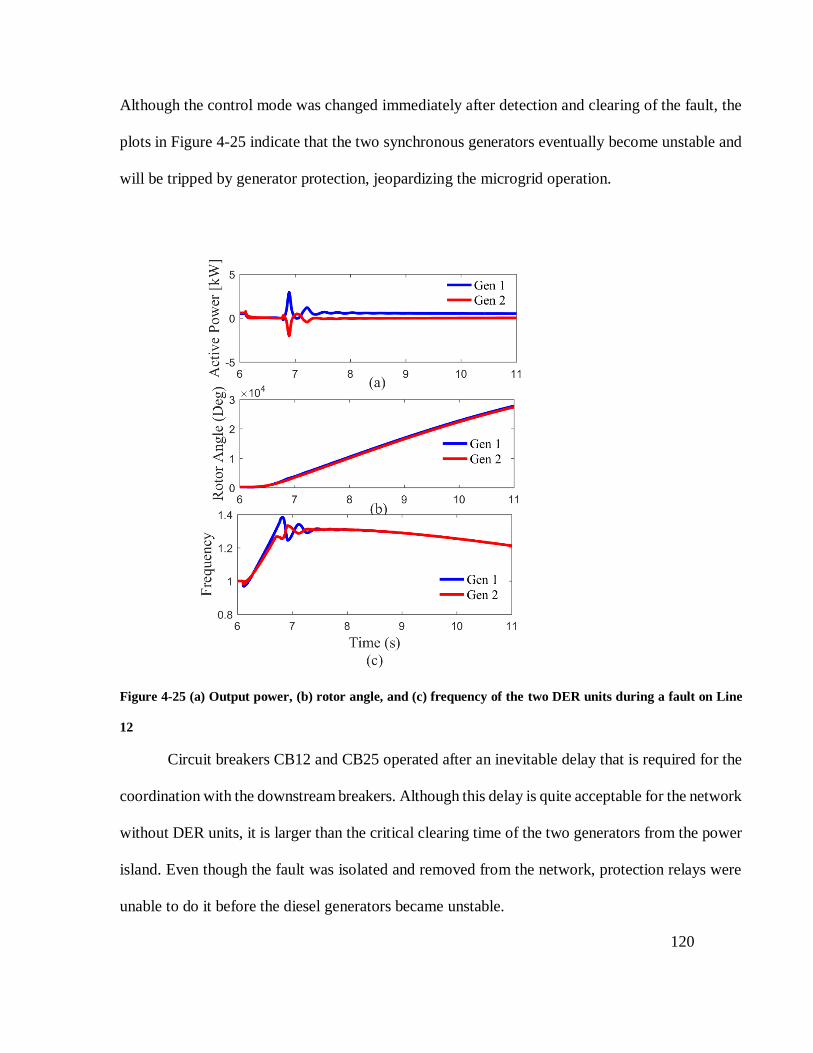
120
Although the control mode was changed immediately after detection and clearing of the fault, the
plots in Figure 4-25 indicate that the two synchronous generators eventually become unstable and
will be tripped by generator protection, jeopardizing the microgrid operation.
Figure 4-25 (a) Output power, (b) rotor angle, and (c) frequency of the two DER units during a fault on Line
12
Circuit breakers CB12 and CB25 operated after an inevitable delay that is required for the
coordination with the downstream breakers. Although this delay is quite acceptable for the network
without DER units, it is larger than the critical clearing time of the two generators from the power
island. Even though the fault was isolated and removed from the network, protection relays were
unable to do it before the diesel generators became unstable.

121
b) Case II: Prolonged fault on Line 23
The second case considers a fault between Bus 2 and Bus 3. The fault needs to be cleared
by removing Line 23 by opening the breaker CB23, and as a result, the loads connected at Bus 3
will not be supplied. After clearing the fault, the two DER units can continue to operate and supply
the load connected to Bus 2 and export excess power to the grid. However, if the opening of relay
CB23 is delayed due to coordination with downstream relays, DER units may become unstable
and tripped by generator protection, especially if the fault is close to Bus 2.
Figure 4-26 shows the generator behavior after a three-phase to ground short circuit on
Line 23 close to Bus 2.
Figure 4-26 (a) Output power, (b) rotor angle, and (3) frequency of the two DER units after a fault on Line 23
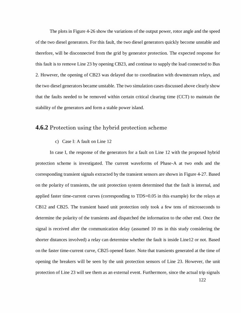
122
The plots in Figure 4-26 show the variations of the output power, rotor angle and the speed
of the two diesel generators. For this fault, the two diesel generators quickly become unstable and
therefore, will be disconnected from the grid by generator protection. The expected response for
this fault is to remove Line 23 by opening CB23, and continue to supply the load connected to Bus
2. However, the opening of CB23 was delayed due to coordination with downstream relays, and
the two diesel generators became unstable. The two simulation cases discussed above clearly show
that the faults needed to be removed within certain critical clearing time (CCT) to maintain the
stability of the generators and form a stable power island.
4.6.2 Protection using the hybrid protection scheme
c) Case I: A fault on Line 12
In case I, the response of the generators for a fault on Line 12 with the proposed hybrid
protection scheme is investigated. The current waveforms of Phase-A at two ends and the
corresponding transient signals extracted by the transient sensors are shown in Figure 4-27. Based
on the polarity of transients, the unit protection system determined that the fault is internal, and
applied faster time-current curves (corresponding to TDS=0.05 in this example) for the relays at
CB12 and CB25. The transient based unit protection only took a few tens of microseconds to
determine the polarity of the transients and dispatched the information to the other end. Once the
signal is received after the communication delay (assumed 10 ms in this study considering the
shorter distances involved) a relay can determine whether the fault is inside Line12 or not. Based
on the faster time-current curve, CB25 opened faster. Note that transients generated at the time of
opening the breakers will be seen by the unit protection sensors of Line 23. However, the unit
protection of Line 23 will see them as an external event. Furthermore, since the actual trip signals

123
are issued by the overcurrent relays, these transients have no adverse effect on the operation of the
protection scheme. Figure 4-27 shows line currents, ferrite coil voltages, filtered ferrite coil
voltages and overcurrent relay trip signals.
Figure 4-27 Operation of the hybrid protection scheme during a fault on Line 21: Phase-A quantities measured
at two ends (a) currents (b) voltages, (c) ferrite core output voltages, (d) filtered coil output voltages (zooned
zoomed view), and (e) decision signals
Figure 4-28 shows the variation of the rotor angles, active power and speed of the two
generators after the fault. Since CB25 was able to remove the fault sooner, DER units managed to
form a stable power island.

124
Figure 4-28 Output power, frequency, and rotor angle of the two DER units with hybrid protection
d) Case II Fault on Line 23
Case II was simulated with the hybrid protection scheme. Following the fault, the transient
based unit protection system quickly found that the fault is within Line 23 and informed the relay
at CB23 to change time-current curve to a faster curve. With faster clearing of the fault by opening
CB23, both DER units were able to remain stable as seen in Figure 4-29 and both DER units
continued to operate in the constant power mode.
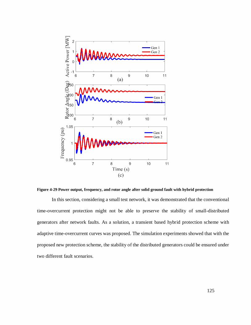
125
Figure 4-29 Power output, frequency, and rotor angle after solid ground fault with hybrid protection
In this section, considering a small test network, it was demonstrated that the conventional
time-overcurrent protection might not be able to preserve the stability of small-distributed
generators after network faults. As a solution, a transient based hybrid protection scheme with
adaptive time-overcurrent curves was proposed. The simulation experiments showed that with the
proposed new protection scheme, the stability of the distributed generators could be ensured under
two different fault scenarios.
126
4.7 Case Study III - Application to 34-bus distribution
network
Figure 4-30 IEEE 34-bus distribution network
In order to demonstrate the viability of the protection concept in a more practical distribution
network, simulation-based investigations were carried out using a modified version of the IEEE
34 bus distribution network [89] shown in Figure 4-30. The modifications to the test circuit was to
add five synchronous distributed generators to the distribution system at 26 kV voltage level. The
details of the DER added are given in Table 4-4. As shown in Figure 4-30, the system is divided
into four protection zones (Zone-A, Zone-B, Zone-C, and Zone-D). The DERs connected to Zone
C and Zone D are designed to operate as independent islands in the case of loss of main supply.
They are capable of providing power to critical loads connected inside each zone and control the
frequency in the island. Depending on the location of the fault, Zone C or Zone D or both Zones
800
806 808 812 814
810
802 850
818
824 826
816
820
822
828 830 854 856
852
832
888 890
838
862
840836860834
842
844
846
848
864
858
800
806 808 812 814
810
802 850
818
824 826
816
820
822
828 830 854 856
852
832
888 890
838
862
840836860834
842
844
846
848
864
858
800
806 808 812 814
810
802 850
818
824 826
816
820
822
828 830 854 856
852
832
888 890
838
862
840836860834
842
844
846
848
864
858
800
806 808 812 814
810
802 850
818
824 826
816
820
822
828 830 854 856
852
832
888 890
838
862
840836860834
842
844
846
848
864
858
800
806 808 812 814
810
802 850
818
824 826
816
820
822
828 830 854 856
852
832
888 890
838
862
840836860834
842
844
846
848
864
858
800
806 808 812 814
810
802 850
818
824 826
816
820
822
828 830 854 856
852
832
888 890
838
862
840836860834
842
844
846
848
864
858
800
806 808 812 814
810
802 850
818
824 826
816
820
822
828 830 854 856
852
832
888 890
838
862
840836860834
842
844
846
848
864
858
DER4
DER5
Zone A
Zone B
Zone C
Zone D
Ferrite coils & Instrument
transformersA
Ferrite coils & Instrument
transformers
DER1
DER2 DER3
F1
F2
CB2
CB3
CB1 CB4

127
C and D can be operated as islanded microgrids. Under the grid-connected mode, these DERs are
operated in constant power mode.
Table 4-4 Details of the DER units added to the IEEE 34 bus feeder
DER Power Rating
(kW)
Connected Bus Zone Type
DER1 20 806 Zone A Sync. Gen.
DER2 170 816 Zone B Sync. Gen.
DER3 800 832 Zone C Sync. Gen.
DER4 400 858 Zone C Sync. Gen.
DER5 850 846 Zone D Sync. Gen.
The conventional protection for the IEEE distribution network was provided with
coordinated overcurrent protection relays. The protection settings were determined considering the
current in-feeds from the DERs. The discrimination margins between adjacent directional
overcurrent relays were kept at 0.2 s. To facilitate transient based fault identification and isolation,
ferrite coil sensors were placed at the boundaries between the zones. The hybrid protection scheme
was developed combining the transient based faulted zone identification and overcurrent
measurements at corresponding zones. In order to investigate the applicability of the proposed
method, faults were simulated at different locations. Results are presented for two different faults,
(i) three-phase fault F1 and (ii) phase-A-to-ground fault F2, simulated inside Zone B. Since the
fault is simulated inside Zone-B, Zone-D and Zone-C can operate as a power island.
Responses of both protection schemes were investigated through detailed simulations
performed in the PSCAD simulation program. Figure 4-31 and Figure 4-32 show the observed
currents and voltages at each end of the protection scheme and the determined transient polarity
128
for fault F1. During the simulations, Zone-B was isolated from the rest of the network upon
detection of the fault by opening breakers CB2 and CB3.
After isolating the fault, frequency, and terminal voltages of the five DER units were
observed. Figure 4-33 to Figure 4-37 compare the voltage and frequency responses of the
generators in the network, followed by the operation of the conventional protection scheme and
the hybrid protection scheme.
Voltage and frequency profiles of DER1, DER3, DER4, and DER5 have been improved
due to the faster operation of the hybrid protection scheme. DER2 is located within the zone where
the fault happens. This means it will be tripped due to the generator protection scheme of DER2.
As it can be observed from the voltage and frequency plots, that the rapid fault identification and
isolation provided by the hybrid protection has helped to improve the voltage and frequency
profiles.

129
Figure 4-31 a),b) Phase A currents at each end (CB2 and CB3) with conventional protection, c),d) Phase A
ferrite coil voltages, e),f) filtered Phase A ferrite coil voltages (Zoomed) , g),h) initial transient direction for
fault F1
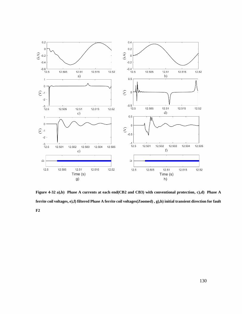
130
Figure 4-32 a),b) Phase A currents at each end(CB2 and CB3) with conventional protection, c),d) Phase A
ferrite coil voltages, e),f) filtered Phase A ferrite coil voltages(Zoomed) , g),h) initial transient direction for fault
F2
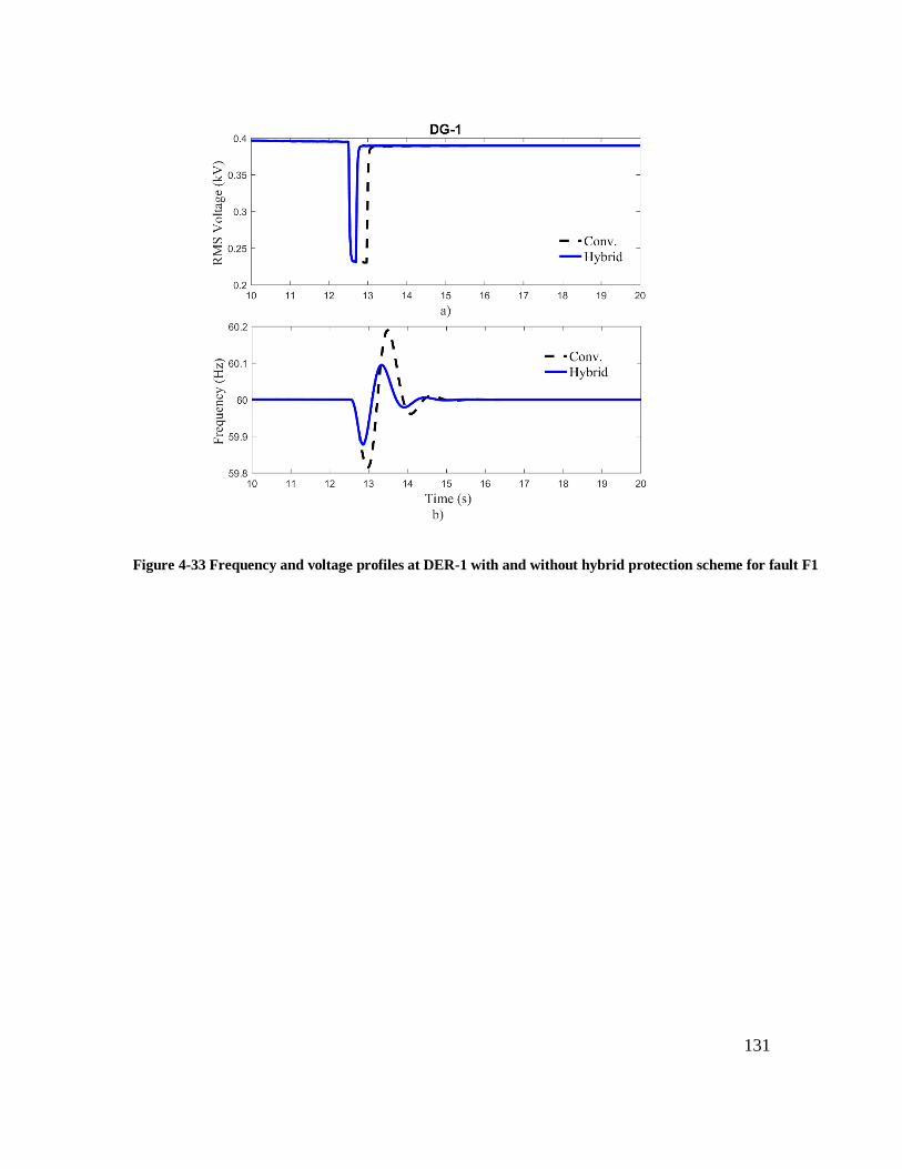
131
Figure 4-33 Frequency and voltage profiles at DER-1 with and without hybrid protection scheme for fault F1
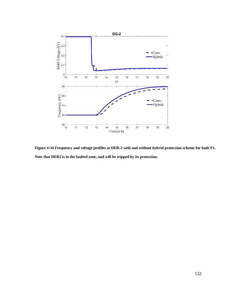
132
Figure 4-34 Frequency and voltage profiles at DER-2 with and without hybrid protection scheme for fault F1.
Note that DER2 is in the faulted zone, and will be tripped by its protection.
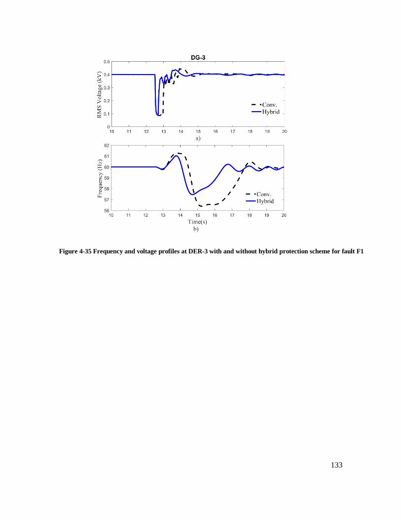
133
Figure 4-35 Frequency and voltage profiles at DER-3 with and without hybrid protection scheme for fault F1

134
Figure 4-36 Frequency and voltage profiles at DER-4 with and without hybrid protection scheme for fault F1
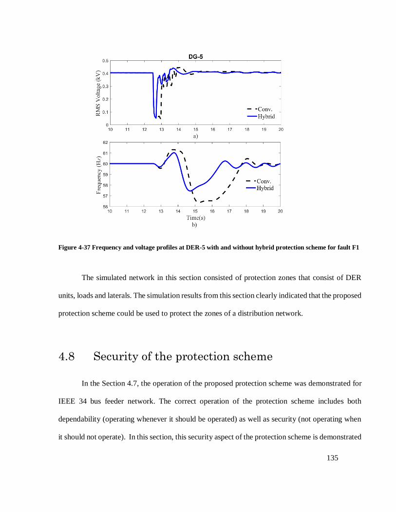
135
Figure 4-37 Frequency and voltage profiles at DER-5 with and without hybrid protection scheme for fault F1
The simulated network in this section consisted of protection zones that consist of DER
units, loads and laterals. The simulation results from this section clearly indicated that the proposed
protection scheme could be used to protect the zones of a distribution network.
4.8 Security of the protection scheme
In the Section 4.7, the operation of the proposed protection scheme was demonstrated for
IEEE 34 bus feeder network. The correct operation of the protection scheme includes both
dependability (operating whenever it should be operated) as well as security (not operating when
it should not operate). In this section, this security aspect of the protection scheme is demonstrated

136
using the test network used in the 3rd case study. The objective of this section is to demonstrate the
ability of the protection scheme to correctly respond to various events happening in the power
network.
4.8.1 Connection of a single-phase lateral
In this simulation case, a single-phase branch with loads was connected to Phase-A at Node
858. Node 858 is located inside the Zone-B. In this scenario, signal waveforms at ends of the
Zone-B should be able to indicate it as an internal incident, while the signal waveforms at other
zone boundaries should indicate an external incident. When the branch connection is far from the
measuring point, the observed transient may be too small to correctly determine the polarity and
will be ignored by the corresponding relays. Figure 4-38 (a), (b), (c), and (d) show Phase-A
currents at the boundary of each zone. When the single-phase distribution segment is connected to
Phase-A of the node 858 of the IEEE 34 bus network, Phase-A currents at the boundaries of Zone-
A and Zone-B changed to accommodate the new load. The currents in the other zones and other
phases (See Appendix C) showed only minor changes in magnitude.

137
Figure 4-38 Phase-A currents measured at zone boundaries and the corresponding filtered ferrite core coil
voltages: (a) & (e) Zone-A; (b) & (f) Zone-B; (c) & (g) Zone-C ; (d) & (h) Zone-D for a single single-phase
branch connection event at t=12.51s. Green and magenta color waveforms are for measurements at DG
terminals in the respective zones. Case: Connection of a single single-phase lateral. See Appendix C for curves
of all three phases.
Appendix C shows the corresponding filtered ferrite coil voltages used to determine the
relative location for other phases. As expected, only the initial polarity of transients observed at
Zone-B boundaries (including those measured at DG boundaries) are the same, meaning the
incident occurred inside Zone-B. However, the corresponding supervisory overcurrent units were
not operated in this scenario, and therefore, no trip signals were issued, although an internal event
e
f
g
h
138
was detected. Furthermore, the other zones either indicated an external event (ex. Zone-C) or
ignored the event due to too small transient magnitudes.
4.8.2 Connection of a generator
In this case, the generator at the node 816 (DER2) was connected to the network by closing
its breaker at t = 12.51 s. Node 816 is located inside Zone-B. Here, the signal waveforms at the
boundary of Zone-B should indicate it as an internal incident, while the signal waveforms at other
zone boundaries should indicate external incident or be unable to classify the event due to
insufficient transient magnitudes.
Figure 4-39(a), (b), (c), and (d) show the currents at the boundary of each zone. When the
generator was connected to node 816 of the IEEE 34 bus network, the phase currents at
measurement points changed due to the incoming current flow to the Zone-B. Figure 4-39(e), (f),
(g), and (h) show the corresponding filtered ferrite coil voltages. In this case, the initial polarity
signals of all the zones are small, meaning the incident will not be detected by the transient based
algorithm, which is reasonable as this is not a fault event.

139
Figure 4-39 Phase-A currents measured at zone boundaries and the corresponding filtered ferrite core coil
voltages: (a) & (e) Zone-A; (b) & (f) Zone-B; (c) & (g) Zone-C ; (d) & (h) Zone-D for a generator connection
event at t=12.51s. Green and magenta color waveforms are for measurements at DG terminals in the respective
zones. Case: Connection of a generator. See Appendix C for curves of all three phases.
4.8.3 Disconnection of a generator
In this case, the generator connected to Node 816 (DER2) is disconnected from the network
by opening its breaker. Node 816 is located inside the Zone-B. Hence, the signal waveforms at the
boundary of the Zone-B should be able to detect it as an internal incident, while the signal
waveforms at other Zone boundaries should indicate as an external incident or unable to detect the
event. Figure 4-40(a), (b), (c), and (d) show the currents at the boundary of each Zone. When the
generator was disconnected, phase currents at the ends of zones slightly changed, however, the
e
g
h
f

140
change was smooth, because the breaker opening happens at the current zero-crossing point.
Figure 4-40(e), (f), (g), and (h) show the corresponding filtered ferrite coil voltages. Since the
opening of the generator breaker did not result in noticeable transients, there is no indication of
any incident happening inside or outside the zone.
Figure 4-40 Phase-A currents measured at zone boundaries and the corresponding filtered ferrite core coil
voltages: (a) & (e) Zone-A; (b) & (f) Zone-B; (c) & (g) Zone-C ; (d) & (h) Zone-D for a generator disconnection
event at t=12.51s. Green and magenta color waveforms are for measurements at DG terminals in the respective
zones. Case: Disconnection of a generator. See Appendix C for the curves of all three phases.
e
f
g
h

141
4.8.4 Three-phase fault
A secure protection scheme means it will not operate for faults outside of the protected
zone. In order to demonstrate that, a three-phase fault was applied at Node 830 which is located
inside the Zone-B. In this scenario, signal waveforms at ends of the Zone-B should be able to
indicate it as an internal incident, while the signal waveforms at other zone boundaries should
indicate an external incident. Figure 4-41 (a), (b), (c), and (d) show Phase-A currents at the
boundary points of each zone (see Appendix C for other phases).
Figure 4-41 Phase-A currents measured at zone boundaries and the corresponding filtered ferrite core coil
voltages: (a) & (e) Zone-A; (b) & (f) Zone-B; (c) & (g) Zone-C ; (d) & (h) Zone-D for a three-phase fault in
Zone-B at t=12.506s. Green and magenta color waveforms are for measurements at DG terminals in the
respective zones. Case: Three phase fault. See Appendix C for the curves of all three phases
e
f
g
h
e
f
g
h

142
Figure 4-41(e), (f), (g), and (h) show the corresponding filtered ferrite coil voltages used
to determine the relative location of the incident. As expected, only the initial polarity of Zone-B
signals are the same, indicating the incident occurred inside Zone-B. The other zones indicate the
incident as external.
4.8.5 Line-Ground Fault
In order to check the security of the protection scheme, a line-ground fault was applied on
Phase-C of Node 830, which is located inside the Zone-B. In this scenario, signal waveforms at
the boundary points of Zone-B should indicate it as an internal incident, while the signal
waveforms at other zone boundaries should indicate it as an external incident. Figure 4-42(a), (b),
(c), and (d) show Phase-C currents at the boundary points of each zone.

143
Figure 4-42 Phase-A currents measured at zone boundaries and the corresponding filtered ferrite core coil
voltages: (a) & (e) Zone-A; (b) & (f) Zone-B; (c) & (g) Zone-C ; (d) & (h) Zone-D for a Phase-C-ground fault
in Zone-B at t=12.506s. Green and magenta color waveforms are for measurements at DG terminals in the
respective zones. Case: Three Three-phase fault. See Appendix C for the curves of all three phases.
Figure 4-42(e), (f), (g), and (h) show the corresponding filtered ferrite coil voltages used
to determine the relative location of the event. As expected, only the initial polarity of Zone-B
signals are the same, showing that the incident occurred inside Zone-B.
Protection scheme was tested for all the fault types and current and ferrite core coil
waveforms for a line-line fault are shown in Appendix C. Observed polarity transients seem to
follow the logic accurately and declare an internal fault for the Zone-B, while the other zones
indicate the incident as external.
e
f
g
h

144
4.9 Faults inside an islanded microgrid
The test network used in Case study III was used to study faults occurring inside an islanded
microgrid that may form after a disturbance. After the three-phase fault described in Section 4.8.4,
Zone-B of the network was isolated by opening the breakers at the boundary of the zone, ie. CB2,
CB3, and the CB of DER-2. Following the isolation from grid supply, Zone-C and Zone-D started
to operate as an islanded microgrid, using DER-4, DER-3 located inside Zone-C, and DER-5
located inside the Zone-D as the power sources. Zone-A is still grid-connected, but has no
connection to the islanded part. The event considered in this scenario is a fault inside Zone-C of
the islanded microgrid. The expected protection response is to de-energize Zone-C and attempt to
operate Zone-D as an islanded microgrid using DER-5. DER-3 and DER-4 will be disconnected
by the protection at generator, or due to the under-voltage or over frequency conditions. In this
case, DER-5 needs to be notified that Zone-D is isolated and requested to take control of the
frequency and voltage inside the newly formed islanded microgrid.
The protection of the microgrid is assumed to be carried out as discussed in Section 4.4. A
three-phase fault was applied between Node 832 and Node 858 in the newly formed microgrid.
The protection scheme should identify this as an internal fault for the Zone-C and open CB4 that
connects Zone-C and Zone-D.
Figure 4-43(a), (b), (c), and (d) show Phase-A current waveforms at the boundary
points of each zone. The current waveforms at boundary points with Zone-B, measured at CB2
and CB3 are zero, because they are open to isolate the Zone-B. Figure 4-43(e), (f), (g), and (h)
show the corresponding filtered ferrite coil voltages. The ferrite coil voltages measured at the open
breaker locations are virtually zero.
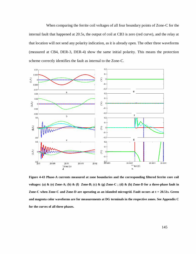
145
When comparing the ferrite coil voltages of all four boundary points of Zone-C for the
internal fault that happened at 20.5s, the output of coil at CB3 is zero (red curve), and the relay at
that location will not send any polarity indication, as it is already open. The other three waveforms
(measured at CB4, DER-3, DER-4) show the same initial polarity. This means the protection
scheme correctly identifies the fault as internal to the Zone-C.
Figure 4-43 Phase-A currents measured at zone boundaries and the corresponding filtered ferrite core coil
voltages: (a) & (e) Zone-A; (b) & (f) Zone-B; (c) & (g) Zone-C ; (d) & (h) Zone-D for a three-phase fault in
Zone-C when Zone-C and Zone-D are operating as an islanded microgrid. Fault occurs at t = 20.51s. Green
and magenta color waveforms are for measurements at DG terminals in the respective zones. See Appendix C
for the curves of all three phases.
e
f
g
h

146
At the same time, the ferrite core coil output voltages at Zone-D boundary indicate that the event
is external. The output voltages of the ferrite core coils at the boundaries of Zone-A and Zone-B
are zero, because these zones are not connected to the faulted part of the distribution system. Once
the overcurrent element confirm the fault, Zone-C was isolated by opening CB4 and opening the
CBs at DER-3 and DER-4.
4.10 Summary
A novel protection scheme that combines the speed of transient based protection with the
security of traditional phasor based protection was proposed to overcome various challenges in
protecting active distribution systems from faults. The operation of the proposed protection scheme
was demonstrated through EMT simulations of a simple power system with DERs as well as with
a modified version of the IEEE 34-bus distribution system.
The first case study demonstrated the basic operation of the proposed protection method
using a simple test network. The next case study demonstrated possible stability issues that can be
overcome by employing the proposed protection method. The third case study demonstrated the
successful application of the proposed protection method for a practical distribution network.
Using the test case III, the security of the transient based protection method is also verified through
simulations for various scenarios.

147

148
Chapter 5 Chapter 5
Implementation of the hybrid protection
scheme
This chapter describes an experimental implementation of the proposed hybrid protection
scheme by integrating the transient based protection with a conventional time overcurrent
protection and testing it through hardware-in-the-loop simulations. The scope of testing is limited
to testing the functionality and generic performance characteristics of a hybrid protection scheme.
The implementation consists of both hardware and software sections, including power system
modeling, sensor designing and programming of the relay. The operation of the hybrid protection
scheme is demonstrated, and the practical limitations are discussed. The content of this chapter is
based on the original work published in [90];
Pathirana, A. Rajapakse, and A. C. Adewole, “Implementation and Testing of a Hybrid Protection
Scheme for Active Distribution Network,” in 2018 IEEE Electrical Power and Energy Conference
(EPEC), 2018, pp. 1–6.
5.1 Introduction
As mentioned during the introductory chapter, power utilities lack the confidence in
Transient Based Protection (TBP) methods due to reasons such as: requirement of complex
149
algorithms, possible training requirements of the models, and the resistance to move away from
protection philosophies which worked for a number of decades. The lack of confidence in power
utilities towards TBP methods may only be overcome by practical demonstrations of such
protection methodologies. Implementing a protection scheme that relies on transient signals in the
laboratory environment and demonstrating its performance using hardware-in-the-loop (HIL)
simulations is a step forward towards achieving that goal.
The TBP method proposed in Chapter 4 does not require any signal comparisons but relies
on the polarity of the transient signals. This method only considers the initial transient polarity of
the current traveling waves. The initial polarity of the current transient can be determined using
the sensor proposed in Chapter 3, which outputs the polarity as two digital signals. The
conventional overcurrent functions and the programmable logic capabilities of a commercial line
protection relay is sufficient to implement the hybrid protection function. The remote and local
polarity signals can be input to the line protection relay as digital inputs.
5.2 Implementation of protection concept
The transients-based protection concept proposed in Chapter 4 relies on the protection
devices located at the boundaries of protected zones in a distribution system. These protection
devices communicate with one another to exchange the fault direction information to identify
whether the fault is inside or outside the protected zone. Figure 5.1 shows the basic arrangement
of this protection scheme.

150
Figure 5-1 Basic arrangement of protection scheme
The protection device/element at each end of the protected segment is capable of
identifying the fault direction using the high-frequency current transients originating from the
fault. Transient polarity detectors based on ferrite core coil sensors discussed in Chapter 3 are used
to detect the polarity of fault-generated high-frequency signals superimposed on phase currents.
The test setup developed for testing the hybrid protection scheme consists of both software
and hardware components. Implementation of the test setup including the hardware prototype of
the hybrid protection scheme is broken down into three steps, namely:
Hardware implementation of the transient polarity detection sensors
Implementation of the hybrid protection on a commercial protective relay by integrating
inputs from transient sensors and appropriate logic programming
Implementation of the power network in RTDS real-time digital simulation platform and
interfacing of the simulator outputs with the hardware relay.

151
5.2.1 Hardware implementation of the sensor
Sensors for detecting the current transients and necessary signal processing components
are implemented in hardware. The main component of the sensor is the ferrite core coil used to
detect the current transients. The next stage is the signal processing stage consisting of protection,
signal scaling, comparators, and logic gates. This section is implemented in hardware as shown in
Figure 5-2.
The ferrite coil used in this implementation consists of only five turns. Its secondary coil
is kept open-circuited. When the ferrite core is not saturated, the output of the coil is proportional
to the rate of change of current going through the coil. Ferrite core is designed such that a slight
saturation is tolerated under power frequency currents. Thus the induced voltages may have a
distorted waveform depending on the primary current level, resulting in a significant amount of
lower order harmonics in the coil output voltage. In order to remove the power frequency and its
lower order harmonics, high-pass filtering of the signal is required before determining the initial
current transient polarity. The induced voltage on the ferrite core coil is fed to the next section of
the sensor hardware. The main components of this stage are protection, filtering, comparators and
latches. Detailed description of the sensor operation and hardware implementation is given in
Chapter 3.

152
Figure 5-2 Circuit used to determine initial transient polarity
5.2.2 Integration of the external protective relay
The next step of the design process of the experimental setup is the integration of the
transient based protection with a conventional digital protective relay. The relay used is an
industrial-grade relay SEL 421. Although SEL 421 is a fully-featured transmission line protection
relay, it was used because it was available in the laboratory. Only its overcurrent functions and
programmable logic were used in the implementation. Inside the SEL421 relay, two over-current
elements with coordinated settings ( TDS=0.23 and TDS=0.05) were implemented. The low-level
CT Secondary Current
Ferrite Core Coil Circuit
Protection
3rd Order High Pass Filter (1 kHz)
-1
1
Threshold
Comparators Latch
Tn
Tp
1st Order Low Pass Filter (200 kHz)
Reset
Optional

153
analog signals representing CT secondary currents were amplified using the Techron current
amplifiers and fed to the SEL 421 relay and ferrite coil sensors located at each end. Digital outputs
(two from each end indicating the polarity of the initial current transient) from the sensor hardware
setups were also inputted to the SEL 421 relay, through digital input ports of the SEL 421.
The logic required to determine whether a fault is inside or outside the protected zone is
implemented in the SEL-421 relay. In this implementation, the same current polarities at both ends
of the protected segment means the fault occurred inside the protected zone/segment. If the relay
determines the fault to be inside the protected segment, the relay can use the overcurrent relay with
the fast settings to trip the breaker without waiting for the coordinated overcurrent delay. Figure
5-3 graphically illustrates this logic implemented in the relay. In Figure 5-3, polarity signals (P,
N) from the remote bus (Bus 2) should be coming through a communication channel.
Figure 5-3 Logic implemented inside SEL421 relay, located at Bus-1
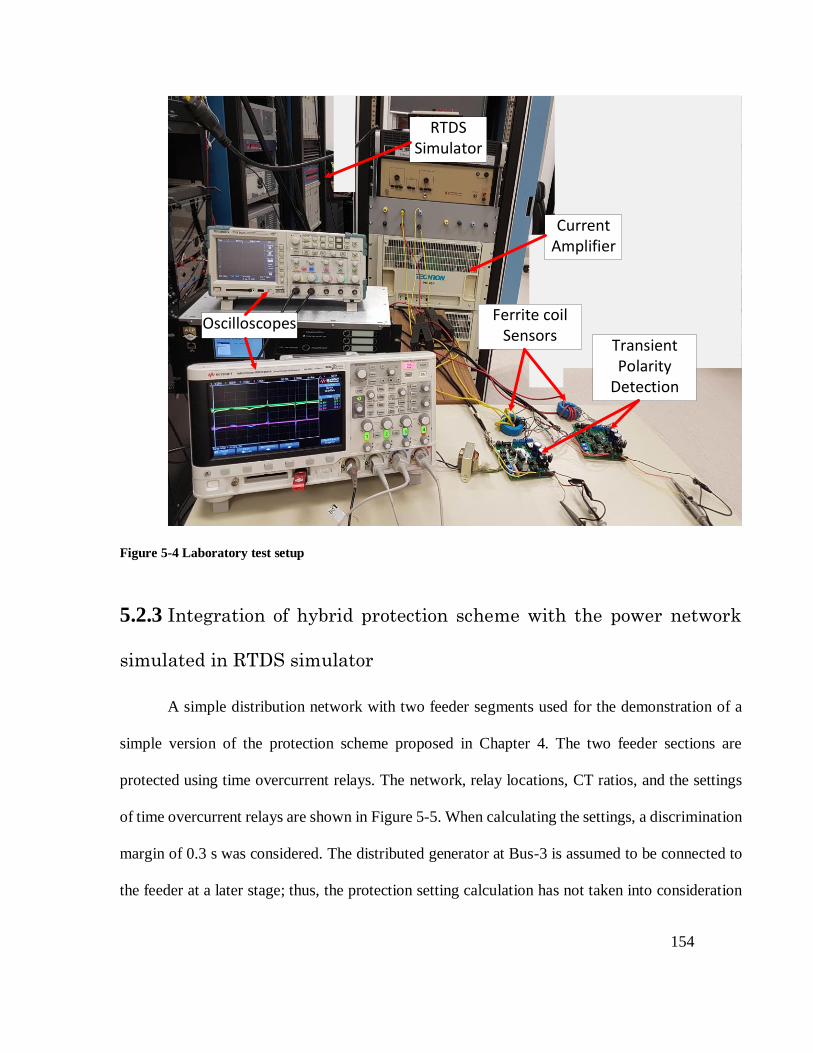
154
Figure 5-4 Laboratory test setup
5.2.3 Integration of hybrid protection scheme with the power network
simulated in RTDS simulator
A simple distribution network with two feeder segments used for the demonstration of a
simple version of the protection scheme proposed in Chapter 4. The two feeder sections are
protected using time overcurrent relays. The network, relay locations, CT ratios, and the settings
of time overcurrent relays are shown in Figure 5-5. When calculating the settings, a discrimination
margin of 0.3 s was considered. The distributed generator at Bus-3 is assumed to be connected to
the feeder at a later stage; thus, the protection setting calculation has not taken into consideration
RTDSSimulator
Ferrite coil Sensors
Current Amplifier
Transient Polarity
Detection
Oscilloscopes

155
the presence of DER. The DER in this test network is a 3 MW synchronous generator driven by a
small steam turbine. The generator is equipped with a standard IEEE rectifier excitation system
for voltage control, and an electro-hydraulic governor with appropriate parameters for both grid-
connected and islanding mode operations.
Fault
15 km 9 km CB3
BUS 1 BUS 2 BUS 3
CT3 Ratio - 200:5IPickUp = 1.54 ATDS = 0.05
CB2CB1
CT2 Ratio - 200:5IPickUp = 1.54 ATDS = 0.16
CT2 Ratio - 400:5IPickUp = 2.325 ATDS = 0.23
Power Grid
DER
GTAO GTDO GTDI GTAO
Current Amplifier
Transient Polarity Detection Sensor
SEL 421 Relay End-1
32 2
Load 1 Load 2
Load 3
Current Amplifier
Transient Polarity Detection Sensor
RTDS
Figure 5-5 Complete protection system implementation
This test network described above was simulated in the RTDS real-time power system
simulation platform for hardware-in-the-loop (HIL) testing. All power system components such
as power sources, breakers, and CTs are implemented using the component models available in
the RTDS master library. Outputs from the CTs are converted into analog signals using GTAO
cards (Analog Output) of RTDS. The analog output signals from the GTAO card are input to a
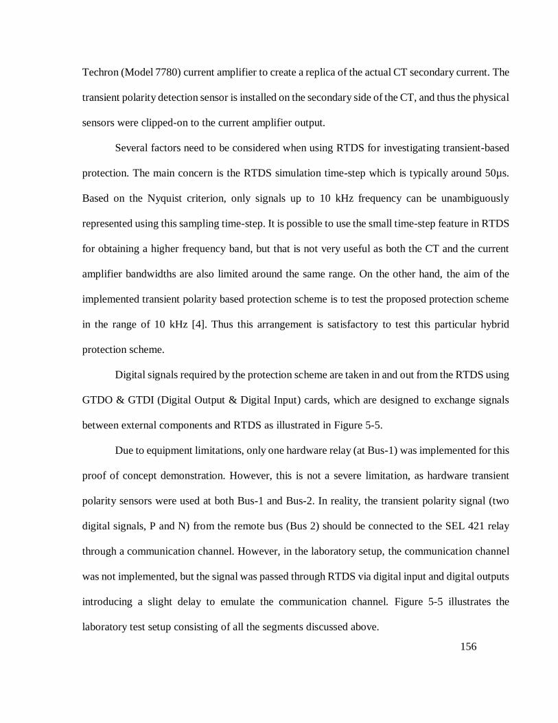
156
Techron (Model 7780) current amplifier to create a replica of the actual CT secondary current. The
transient polarity detection sensor is installed on the secondary side of the CT, and thus the physical
sensors were clipped-on to the current amplifier output.
Several factors need to be considered when using RTDS for investigating transient-based
protection. The main concern is the RTDS simulation time-step which is typically around 50µs.
Based on the Nyquist criterion, only signals up to 10 kHz frequency can be unambiguously
represented using this sampling time-step. It is possible to use the small time-step feature in RTDS
for obtaining a higher frequency band, but that is not very useful as both the CT and the current
amplifier bandwidths are also limited around the same range. On the other hand, the aim of the
implemented transient polarity based protection scheme is to test the proposed protection scheme
in the range of 10 kHz [4]. Thus this arrangement is satisfactory to test this particular hybrid
protection scheme.
Digital signals required by the protection scheme are taken in and out from the RTDS using
GTDO & GTDI (Digital Output & Digital Input) cards, which are designed to exchange signals
between external components and RTDS as illustrated in Figure 5-5.
Due to equipment limitations, only one hardware relay (at Bus-1) was implemented for this
proof of concept demonstration. However, this is not a severe limitation, as hardware transient
polarity sensors were used at both Bus-1 and Bus-2. In reality, the transient polarity signal (two
digital signals, P and N) from the remote bus (Bus 2) should be connected to the SEL 421 relay
through a communication channel. However, in the laboratory setup, the communication channel
was not implemented, but the signal was passed through RTDS via digital input and digital outputs
introducing a slight delay to emulate the communication channel. Figure 5-5 illustrates the
laboratory test setup consisting of all the segments discussed above.

157
5.3 Results & discussion
Some of the test results are presented in this section to demonstrate the operation of the
implemented hybrid protection scheme. Two scenarios, including an internal fault and an external
fault, are considered.
5.3.1 Internal Fault
First, a test was carried-out without the use of a hybrid protection scheme. In the test
network shown in Figure 5-5, a solid three-phase-to-ground fault is applied between Bus 1 and Bus
2 at 12 km from Bus 1. Figure 5-6 shows the line currents (Phase-A) and corresponding CT
secondary currents at each end of the protected segment. CT secondary currents are fed to SEL-
421 relay. A trip signal is issued from the coordinated time overcurrent function after about 0.58 s
delay, as indicated by the SEL-421 relay recordings shown in Figure 5-7. In Figure 5-7 the issued trip
signal is labelled as 51S1T.
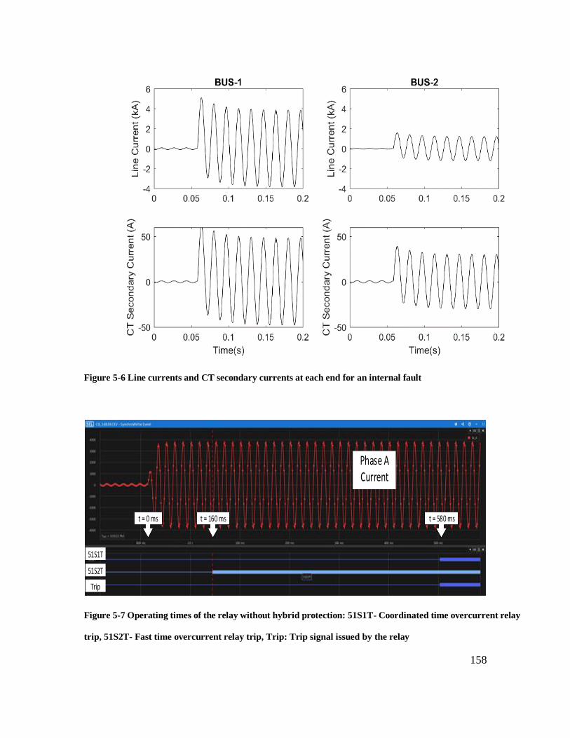
158
Figure 5-6 Line currents and CT secondary currents at each end for an internal fault
Figure 5-7 Operating times of the relay without hybrid protection: 51S1T- Coordinated time overcurrent relay
trip, 51S2T- Fast time overcurrent relay trip, Trip: Trip signal issued by the relay
Phase ACurrent
t = 0 ms
51S1T
Trip
51S2T
t = 160 ms t = 580 ms

159
Then the hybrid protection scheme is enabled and the same fault is applied again. For the
same fault, output from the ferrite core sensor and filtered ferrite coil response at both ends is
plotted in Figure 5-8.
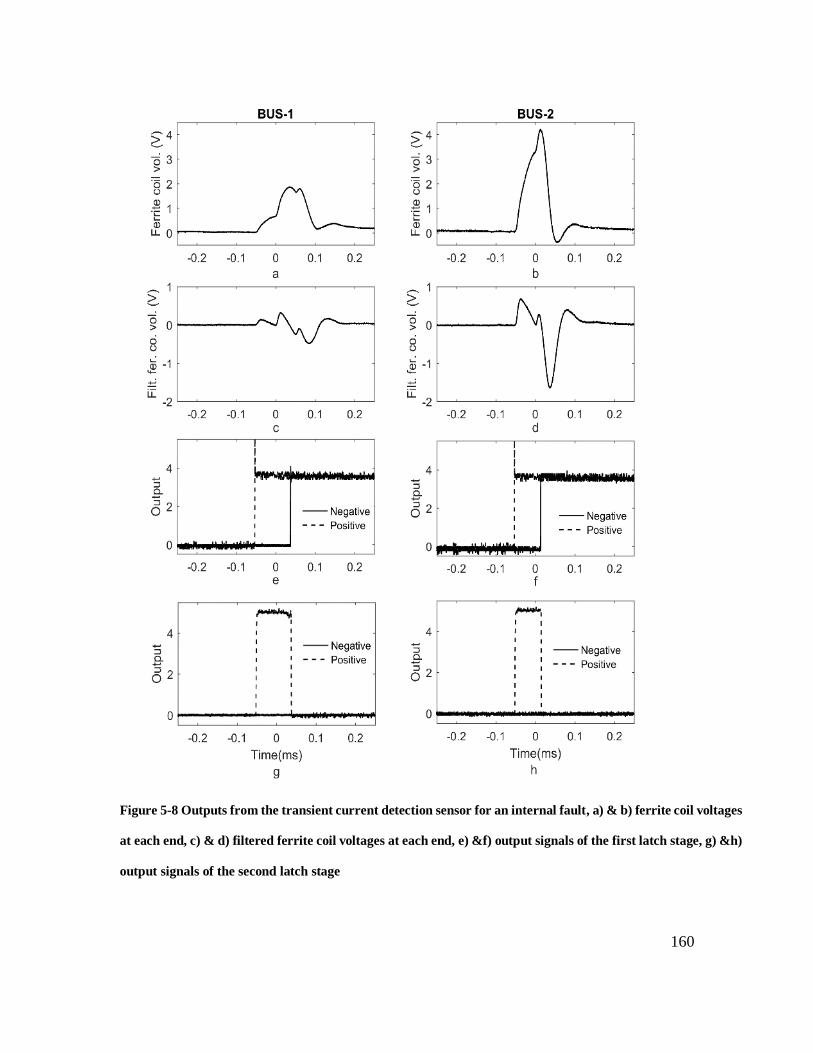
160
Figure 5-8 Outputs from the transient current detection sensor for an internal fault, a) & b) ferrite coil voltages
at each end, c) & d) filtered ferrite coil voltages at each end, e) &f) output signals of the first latch stage, g) &h)
output signals of the second latch stage
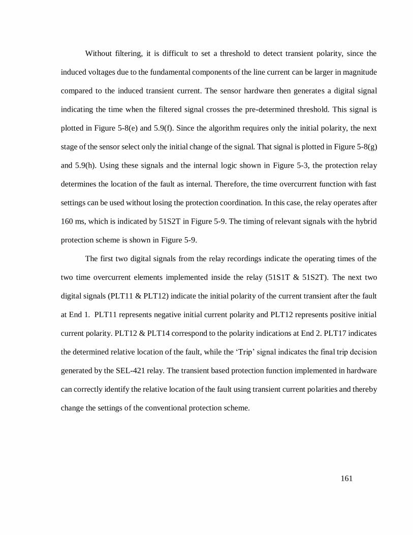
161
Without filtering, it is difficult to set a threshold to detect transient polarity, since the
induced voltages due to the fundamental components of the line current can be larger in magnitude
compared to the induced transient current. The sensor hardware then generates a digital signal
indicating the time when the filtered signal crosses the pre-determined threshold. This signal is
plotted in Figure 5-8(e) and 5.9(f). Since the algorithm requires only the initial polarity, the next
stage of the sensor select only the initial change of the signal. That signal is plotted in Figure 5-8(g)
and 5.9(h). Using these signals and the internal logic shown in Figure 5-3, the protection relay
determines the location of the fault as internal. Therefore, the time overcurrent function with fast
settings can be used without losing the protection coordination. In this case, the relay operates after
160 ms, which is indicated by 51S2T in Figure 5-9. The timing of relevant signals with the hybrid
protection scheme is shown in Figure 5-9.
The first two digital signals from the relay recordings indicate the operating times of the
two time overcurrent elements implemented inside the relay (51S1T & 51S2T). The next two
digital signals (PLT11 & PLT12) indicate the initial polarity of the current transient after the fault
at End 1. PLT11 represents negative initial current polarity and PLT12 represents positive initial
current polarity. PLT12 & PLT14 correspond to the polarity indications at End 2. PLT17 indicates
the determined relative location of the fault, while the ‘Trip’ signal indicates the final trip decision
generated by the SEL-421 relay. The transient based protection function implemented in hardware
can correctly identify the relative location of the fault using transient current polarities and thereby
change the settings of the conventional protection scheme.
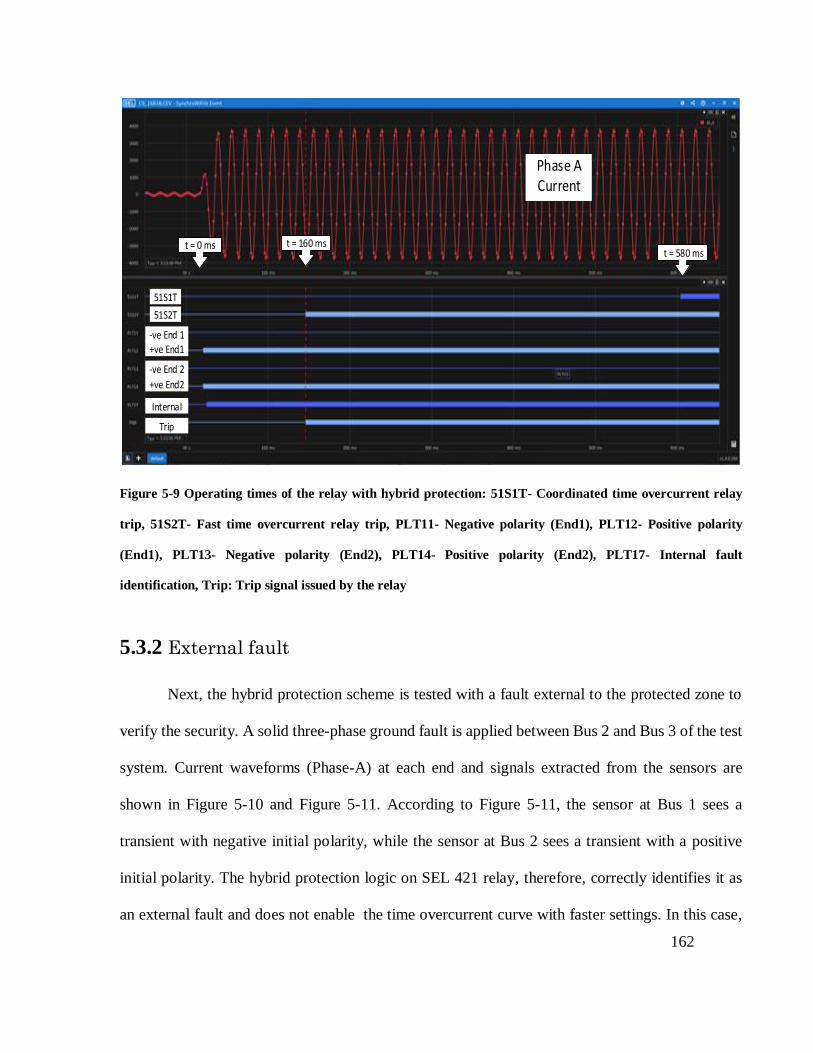
162
Phase ACurrent
t = 0 ms
51S1T
51S2T
t = 160 mst = 580 ms
-ve End 1+ve End1
-ve End 2
+ve End2
Internal FaultTrip
Figure 5-9 Operating times of the relay with hybrid protection: 51S1T- Coordinated time overcurrent relay
trip, 51S2T- Fast time overcurrent relay trip, PLT11- Negative polarity (End1), PLT12- Positive polarity
(End1), PLT13- Negative polarity (End2), PLT14- Positive polarity (End2), PLT17- Internal fault
identification, Trip: Trip signal issued by the relay
5.3.2 External fault
Next, the hybrid protection scheme is tested with a fault external to the protected zone to
verify the security. A solid three-phase ground fault is applied between Bus 2 and Bus 3 of the test
system. Current waveforms (Phase-A) at each end and signals extracted from the sensors are
shown in Figure 5-10 and Figure 5-11. According to Figure 5-11, the sensor at Bus 1 sees a
transient with negative initial polarity, while the sensor at Bus 2 sees a transient with a positive
initial polarity. The hybrid protection logic on SEL 421 relay, therefore, correctly identifies it as
an external fault and does not enable the time overcurrent curve with faster settings. In this case,
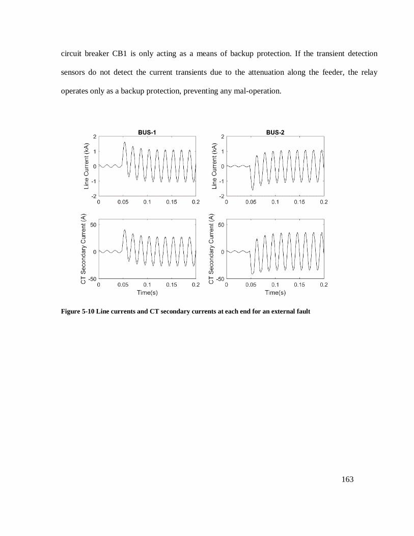
163
circuit breaker CB1 is only acting as a means of backup protection. If the transient detection
sensors do not detect the current transients due to the attenuation along the feeder, the relay
operates only as a backup protection, preventing any mal-operation.
Figure 5-10 Line currents and CT secondary currents at each end for an external fault

164
Figure 5-11 Outputs from the transient current detection sensor for an external fault
5.4 Summary
Hardware implantation of the proposed hybrid protection scheme consisting of transient
polarity comparison and time-overcurrent function demonstrated the viability of practical
implementation of the proposed algorithm with simple modification to a conventional relay. HIL
simulation with Real Time Digital Simulator demonstrated the correct functioning of the proposed
hybrid relay in a simple distribution feeder protection scheme. Implementation of a hybrid
protection scheme in the laboratory and demonstration of its performance is expected to enhance
the confidence of the power industry towards the use of transient based protection methods.
Furthermore, successful implementation of this protection scheme demonstrated that transient
based protection methods could be implemented for distribution networks without any special
relays that require sampling frequencies in the megahertz range.

165
166
Chapter 6 Chapter 6
Conclusions and future work
This chapter concludes the thesis by discussing the major contributions of the research on
the protection of active distribution networks using hybrid principles and recommendations for
future research.
6.1 Conclusions
The interconnection of distributed energy resources alters the radial structure of
distribution systems and the character of fault currents making the protection of active distribution
systems a challenging problem. In Chapter 2, these challenges were discussed in detail, and the
potential solutions that have been proposed were critically examined. The necessity for improved
and more effective solutions to the problem of protection of active distribution systems was
recognized.
In Chapter 3, a novel sensor based on a ferrite core coil was proposed to measure current
transients and determine their polarities for protection purposes. An electronic circuit to implement
the proposed sensor system was designed and fabricated. An electromagnetic transient simulation
model of the sensor was also developed and implemented in PSCAD software. During this process,
a new mathematical model to incorporate the dynamic characteristics of the BH curve of a ferrite
core was developed. This dynamic hysteresis model of the ferrite core was validated using the
experimental results obtained in the laboratory. Chapter 3 also compared the effectiveness of the
167
proposed sensor system with two digital signal processing based transient detection approaches,
namely discrete wavelet transform and mathematical morphology. The research presented in this
chapter showed that the proposed analog measurement circuit could detect the transients and
determine their polarities more robustly and reliably. The experiments confirmed the validity of
the proposed model for sensor system including its ability to represent the dynamic hysteresis
characteristics of a ferrite core and produce reasonably accurate output voltage waveforms. The
comparisons of the proposed sensor performance with the digital signal processing approaches
highlighted the superiority of the proposed analog measurement approach under noisy and
challenging conditions. By implementing a new sensor and developing a model to simulate the
sensor, this part of the thesis laid the foundation for using current transients and their polarities for
protection applications.
The next chapter of the thesis was devoted to investigate a novel protection scheme to
overcome various challenges in protecting active distribution systems from faults. The core
principle of the proposed method was to identify the faulty section by comparing the polarities of
the current transients measured at two or more locations on the boundary of the protected zone. A
conventional protection function was applied to supervise this transient based faulted segment
identification algorithm to improve the security of protection. Through this hybrid protection
approach, it was possible to eliminate the coordination delays associated with the traditional
overcurrent protection methods. Chapter 4 examined the application of the transient based
protection algorithm in conjunction with overcurrent and distance protection. After detailing the
logic and application of the proposed method, the operation of the protection scheme was
demonstrated through EMT simulations of two small power networks and a modified version of
the IEEE 34-bus distribution system.

168
Simulations of the first simple active distribution network demonstrated the correct
function of the proposed hybrid protection and benefits of the faster protection it can bring: The
faster protection resulted in improved voltage and frequency profiles in microgrids when islanded.
The next case study demonstrated the stability of small low inertia synchronous distributed
generators can be improved by employing a faster protection method such as the proposed one.
The results obtained with the IEEE 34 bus distribution system also confirmed that rapid isolation
of faults lead to improved voltage and frequency profiles, and demonstrated the applicability of
the proposed method for larger scale distribution systems. The studies also confirmed the security
of the proposed hybrid protection method under various types of fault and non-fault events.
Simulation experiments with all three test systems showed that the proposed protection scheme
could be successfully applied to improve the reliability and speed of protection.
Chapter 5 of the thesis covers the practical implementation of the protection scheme. A
hardware in the loop simulation setup was developed using an RTDS real-time simulator to
implement a power system. The transient sensors fabricated in Chapter 3, and a commercial relay
was used in the HIL simulation setup. The operation of the protection algorithm was successfully
verified for a set of cases, and the practicality of applying transient based methods for protection
was demonstrated in a limited manner.
6.2 Contributions
The main contributions of the research include
A simple sensing arrangement based on a ferrite core coil and associated electronics
for detecting high-frequency transients in currents and their initial polarities.
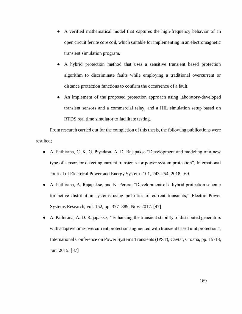
169
A verified mathematical model that captures the high-frequency behavior of an
open circuit ferrite core coil, which suitable for implementing in an electromagnetic
transient simulation program.
A hybrid protection method that uses a sensitive transient based protection
algorithm to discriminate faults while employing a traditional overcurrent or
distance protection functions to confirm the occurrence of a fault.
An implement of the proposed protection approach using laboratory-developed
transient sensors and a commercial relay, and a HIL simulation setup based on
RTDS real time simulator to facilitate testing.
From research carried out for the completion of this thesis, the following publications were
resulted;
A. Pathirana, C. K. G. Piyadasa, A. D. Rajapakse “Development and modeling of a new
type of sensor for detecting current transients for power system protection”, International
Journal of Electrical Power and Energy Systems 101, 243-254, 2018. [69]
A. Pathirana, A. Rajapakse, and N. Perera, “Development of a hybrid protection scheme
for active distribution systems using polarities of current transients,” Electric Power
Systems Research, vol. 152, pp. 377–389, Nov. 2017. [47]
A. Pathirana, A. D. Rajapakse, “Enhancing the transient stability of distributed generators
with adaptive time-overcurrent protection augmented with transient based unit protection”,
International Conference on Power Systems Transients (IPST), Cavtat, Croatia, pp. 15-18,
Jun. 2015. [87]

170
A. Pathirana, A. Rajapakse, and A. C. Adewole, “Implementation and Testing of a Hybrid
Protection Scheme for Active Distribution Network,” in 2018 IEEE Electrical Power and
Energy Conference (EPEC), 2018, pp. 1–6.[90]
6.3 Future work
The current research examined the operation of the hybrid protection algorithm mainly
with synchronous generator based DER. Operation of the transient based protection scheme with
inverter interfaced distributed generators needs to be investigated. Although the communication
bandwidth requirements for the proposed approach is minimal, the impact of communication
delays and congestion need to be investigated. The use of transient based protection to identify the
fault region can be used with other protection mechanisms for improved performance.
Estimation of the dynamic model parameters of the ferrite core coil was carried out using
a trial and error method. The systematic method of model parameter estimation needs to be
investigated.In RTDS implementation, due to equipment and technical limitations, only a small
network was implemented for the proof of concept demonstration. A more robust relay
implementation of the protection approach should be tested with a more extensive network
implemented in RTDS with different kinds of DER units, followed by appropriate field testing.
More detailed investigations into the sensitivity of the proposed protection scheme for
different types of networks and operating conditions will provide further confidence on the
proposed hybrid approach before possible real world implementations.

171
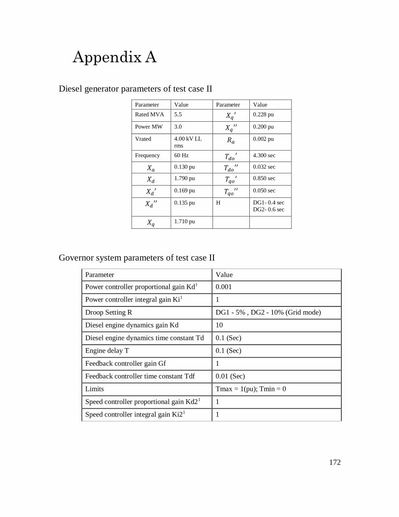
172
Appendix A
Diesel generator parameters of test case II
Parameter Value Parameter Value
Rated MVA 5.5 𝑋𝑞′ 0.228 pu
Power MW 3.0 𝑋𝑞′′ 0.200 pu
Vrated 4.00 kV LL
rms 𝑅𝑎 0.002 pu
Frequency 60 Hz 𝑇𝑑𝑜′ 4.300 sec
𝑋𝑎 0.130 pu 𝑇𝑑𝑜 ′′ 0.032 sec
𝑋𝑑 1.790 pu 𝑇𝑞𝑜′ 0.850 sec
𝑋𝑑′ 0.169 pu 𝑇𝑞𝑜′′ 0.050 sec
𝑋𝑑′′ 0.135 pu H DG1- 0.4 sec
DG2- 0.6 sec
𝑋𝑞 1.710 pu
Governor system parameters of test case II
Parameter Value
Power controller proportional gain Kd1 0.001
Power controller integral gain Ki1 1
Droop Setting R DG1 - 5% , DG2 - 10% (Grid mode)
Diesel engine dynamics gain Kd 10
Diesel engine dynamics time constant Td 0.1 (Sec)
Engine delay T 0.1 (Sec)
Feedback controller gain Gf 1
Feedback controller time constant Tdf 0.01 (Sec)
Limits Tmax = 1(pu); Tmin = 0
Speed controller proportional gain Kd21 1
Speed controller integral gain Ki21 1
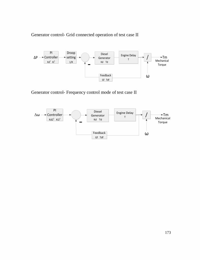
173
Generator control- Grid connected operation of test case II
PI Controller
Kd1 Ki1
Diesel Generator
Kd Td
/
Feedback
Gf Tdf
-Tm
ω
Droop setting
1/R Mechanical Torque
∆PEngine Delay
T
Generator control- Frequency control mode of test case II
∆ωPI
ControllerKd21 Ki21
Diesel Generator
Kd Td
/
Feedback
Gf Tdf
-Tm
ω
Mechanical Torque
Engine DelayT

174
Appendix B
IEEE 34 node test feeder configuration and parameters of test case III
Overhead Line Configurations (Config.)
Config. Phasing Phase Neutral Spacing ID
ACSR ACSR
300 B A C N 1/0 1/0 500
301 B A C N #2 6/1 #2 6/1 500
302 A N #4 6/1 #4 6/1 510
303 B N #4 6/1 #4 6/1 510
304 B N #2 6/1 #2 6/1 510
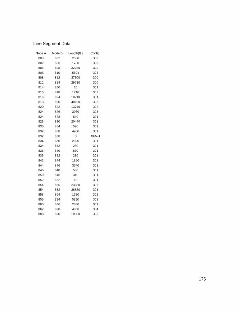
175
Line Segment Data
Node A Node B Length(ft.) Config. 800 802 2580 300 802 806 1730 300 806 808 32230 300 808 810 5804 303 808 812 37500 300 812 814 29730 300 814 850 10 301 816 818 1710 302 816 824 10210 301 818 820 48150 302 820 822 13740 302 824 826 3030 303 824 828 840 301 828 830 20440 301 830 854 520 301 832 858 4900 301 832 888 0 XFM-1 834 860 2020 301 834 842 280 301 836 840 860 301 836 862 280 301 842 844 1350 301 844 846 3640 301 846 848 530 301 850 816 310 301 852 832 10 301 854 856 23330 303 854 852 36830 301 858 864 1620 302 858 834 5830 301 860 836 2680 301 862 838 4860 304 888 890 10560 300

176
Transformer Data
kVA kV-high kV-low R - % X - %
Substation: 2500 69 - D 24.9 -Gr. W 1 8
XFM -1 500 24.9 - Gr.W 4.16 - Gr. W 1.9 4.08
Spot Loads
Node Load Ph-1 Ph-1 Ph-2 Ph-2 Ph-3 Ph-4
Model kW kVAr kW kVAr kW kVAr
860 Y-PQ 20 16 20 16 20 16
840 Y-I 9 7 9 7 9 7
844 Y-Z 135 105 135 105 135 105
848 D-PQ 20 16 20 16 20 16
890 D-I 150 75 150 75 150 75
830 D-Z 10 5 10 5 25 10
Total 344 224 344 224 359 229
Distributed Loads
Node Node Load Ph-1 Ph-1 Ph-2 Ph-2 Ph-3 Ph-3
A B Model kW kVAr kW kVAr kW kVAr
802 806 Y-PQ 0 0 30 15 25 14
808 810 Y-I 0 0 16 8 0 0
818 820 Y-Z 34 17 0 0 0 0
820 822 Y-PQ 135 70 0 0 0 0
816 824 D-I 0 0 5 2 0 0
824 826 Y-I 0 0 40 20 0 0
824 828 Y-PQ 0 0 0 0 4 2
828 830 Y-PQ 7 3 0 0 0 0
854 856 Y-PQ 0 0 4 2 0 0
832 858 D-Z 7 3 2 1 6 3
858 864 Y-PQ 2 1 0 0 0 0
858 834 D-PQ 4 2 15 8 13 7
834 860 D-Z 16 8 20 10 110 55
860 836 D-PQ 30 15 10 6 42 22
836 840 D-I 18 9 22 11 0 0
862 838 Y-PQ 0 0 28 14 0 0
842 844 Y-PQ 9 5 0 0 0 0
844 846 Y-PQ 0 0 25 12 20 11
846 848 Y-PQ 0 0 23 11 0 0
Total 262 133 240 120 220 114

177
Shunt Capacitors
Node Ph-A Ph-B Ph-C
kVAr kVAr kVAr
844 100 100 100
848 150 150 150
Total 250 250 250

178
Appendix C
Figure C-1) Currents at each end of Zone-A b) Currents at each end of Zone-B c) Currents at each end of Zone-C d)
Currents at each end of Zone-D for single phase branch connection at t=12.51s for connection of a single phase lateral.
There columns of plots are for three phases. Green and magenta color waveforms are for generator terminal
measurements
Figure C-2 a) Filtered ferrite coil voltages at each end of Zone-A b) Filtered ferrite coil voltages at each end of Zone-B c)
Filtered ferrite coil voltages at each end of Zone-C d) Filtered ferrite coil voltages at each end of Zone-D for single phase
branch connection at t=12.51s for connection of a single phase lateral. There columns of plots are for three phases. Green
and magenta color waveforms are for generator terminal measurements
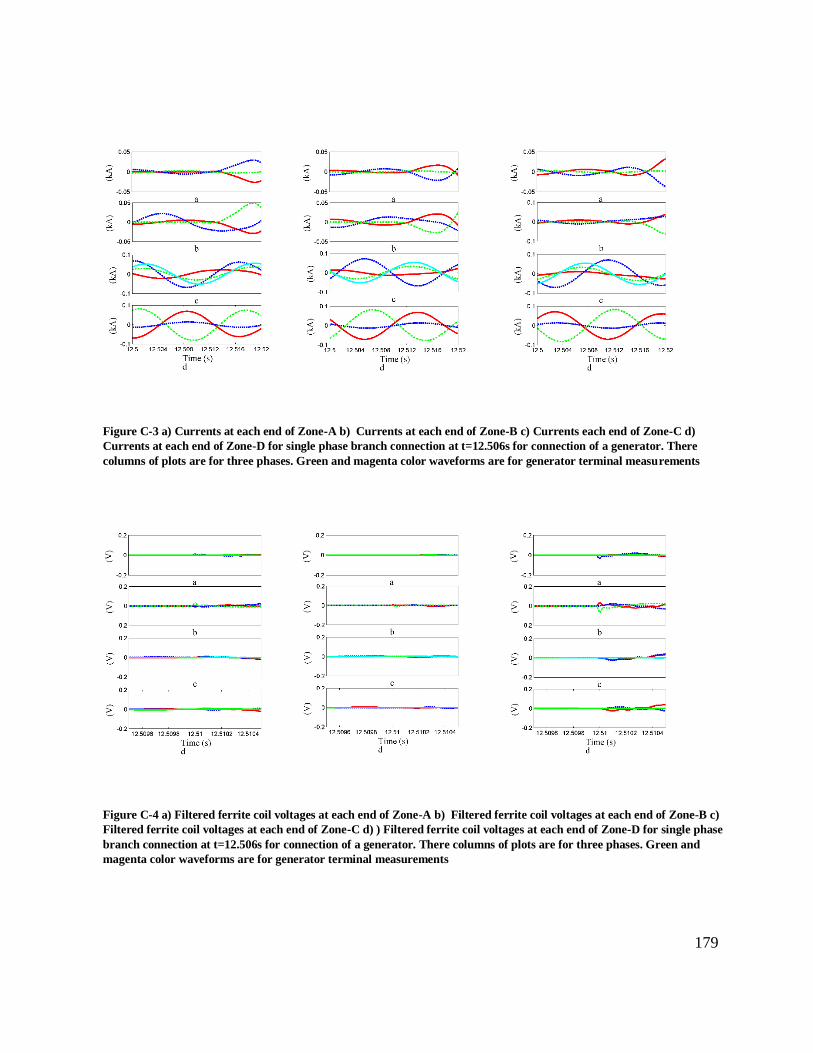
179
Figure C-3 a) Currents at each end of Zone-A b) Currents at each end of Zone-B c) Currents each end of Zone-C d)
Currents at each end of Zone-D for single phase branch connection at t=12.506s for connection of a generator. There
columns of plots are for three phases. Green and magenta color waveforms are for generator terminal measurements
Figure C-4 a) Filtered ferrite coil voltages at each end of Zone-A b) Filtered ferrite coil voltages at each end of Zone-B c)
Filtered ferrite coil voltages at each end of Zone-C d) ) Filtered ferrite coil voltages at each end of Zone-D for single phase
branch connection at t=12.506s for connection of a generator. There columns of plots are for three phases. Green and
magenta color waveforms are for generator terminal measurements

180
Figure C-5 a) Currents at each end of Zone-A b) Currents at each end of Zone-B c) Currents each end of Zone-C d)
Currents at each end of Zone-D for single phase branch connection at t=12.506s for disconnection of a generator. There
columns of plots are for three phases. Green and magenta color waveforms are for generator terminal measurements
Figure C-6 a) Filtered ferrite coil voltages at each end of Zone-A b) Filtered ferrite coil voltages at each end of Zone-B c)
Filtered ferrite coil voltages at each end of Zone-C d) ) Filtered ferrite coil voltages at each end of Zone-D for single phase
branch connection at t=12.506s for disconnection of a generator. There columns of plots are for three phases. Green and
magenta color waveforms are for generator terminal measurements

181
Figure C-7 a) Currents at each end of Zone-A b) Currents at each end of Zone-B c) Currents at each end of Zone-C d) )
Currents at each end of Zone-D for single phase branch connection at t=12.506s for three phase fault. There columns of
plots are for three phases. Green and magenta color waveforms are for generator terminal measurements.
Figure C-8 a) Filtered ferrite coil voltages at each end of Zone-A b) Filtered ferrite coil voltages at each end of Zone-B c)
Filtered ferrite coil voltages at each end of Zone-C d) Filtered ferrite coil voltages at each end of Zone-D for single phase
branch connection at t=12.506s for three phase fault. There columns of plots are for three phases. Green and magenta
color waveforms are for generator terminal measurements.

182
Figure C-9 a) Currents at each end of Zone-A b) Currents at each end of Zone-B c) Currents at each end of Zone-C d)
Currents at each end of Zone-D for single phase branch connection at t=12.506s for line-line fault. There columns of plots
are for three phases. Green and magenta color waveforms are for generator terminal measurements.
Figure C-10 a) Filtered ferrite coil voltages at each end of Zone-A b) Filtered ferrite coil voltages at each end of Zone-B c)
Filtered ferrite coil voltages at each end of Zone-C d) Filtered ferrite coil voltages at each end of Zone-D for single phase
branch connection at t=12.506s for line-line fault. There columns of plots are for three phases. Green and magenta color
waveforms are for generator terminal measurements
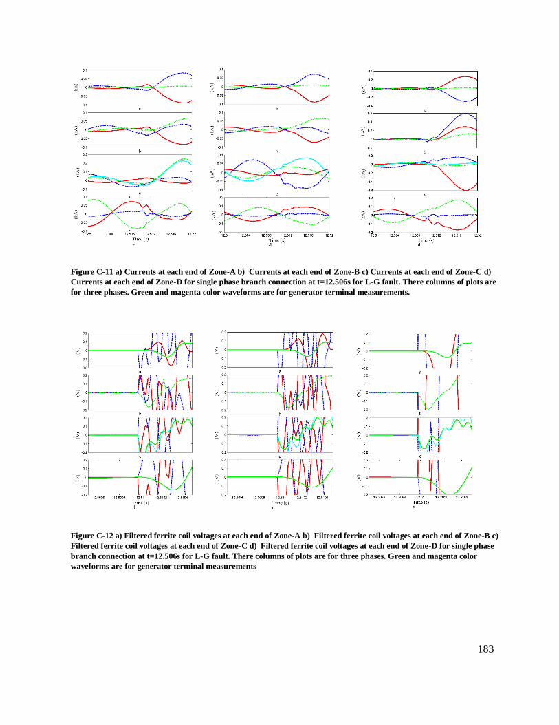
183
Figure C-11 a) Currents at each end of Zone-A b) Currents at each end of Zone-B c) Currents at each end of Zone-C d)
Currents at each end of Zone-D for single phase branch connection at t=12.506s for L-G fault. There columns of plots are
for three phases. Green and magenta color waveforms are for generator terminal measurements.
Figure C-12 a) Filtered ferrite coil voltages at each end of Zone-A b) Filtered ferrite coil voltages at each end of Zone-B c)
Filtered ferrite coil voltages at each end of Zone-C d) Filtered ferrite coil voltages at each end of Zone-D for single phase
branch connection at t=12.506s for L-G fault. There columns of plots are for three phases. Green and magenta color
waveforms are for generator terminal measurements
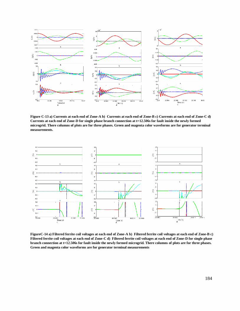
184
Figure C-13 a) Currents at each end of Zone-A b) Currents at each end of Zone-B c) Currents at each end of Zone-C d)
Currents at each end of Zone-D for single phase branch connection at t=12.506s for fault inside the newly formed
microgrid. There columns of plots are for three phases. Green and magenta color waveforms are for generator terminal
measurements.
FigureC-14 a) Filtered ferrite coil voltages at each end of Zone-A b) Filtered ferrite coil voltages at each end of Zone-B c)
Filtered ferrite coil voltages at each end of Zone-C d) Filtered ferrite coil voltages at each end of Zone-D for single phase
branch connection at t=12.506s for fault inside the newly formed microgrid. There columns of plots are for three phases.
Green and magenta color waveforms are for generator terminal measurements

185

186
References
[1] Federal Energy Regulatory Commission, “Office of Energy Projects Energy
Infrastructure Update,” Jun. 2015. [2] “Office of Energy Projects Energy Infrastructure Update,” Dec. 2014.
[3] “Renewable energy in Europe 2017 — Recent growth and knock-on effects,” European
Environment Agency. [Online]. Available: https://www.eea.europa.eu/publications/.
[Accessed: 05-Jun-2018].
[4] P. Gomes, A. C. B. Martins, C. R. Zani, and S. L. A. Sardinha, “Connection requirements
and Grid Codes for distributed generation,” CIGRE/IEEE PES Joint Symposium
Integration of Wide-Scale Renewable Resources Into the Power Delivery System, United
states of America, 2009.
[5] A. F. Zobaa and C. Cecati, “A comprehensive review on distributed power generation,”
International Symposium on Power Electronics, Electrical Drives, Automation and
Motion, 2006.
[6] “IEEE Guide for Design, Operation, and Integration of Distributed Resource Island
Systems with Electric Power Systems,” IEEE Std 1547.4-2011, Jul. 2011.
[7] “IEEE Standard for Interconnection and Interoperability of Distributed Energy
Resources with Associated Electric Power Systems Interfaces,” IEEE Std 1547-2018, Apr.
2018.
[8] “SEL-T400L Time-Domain Line Protection | Schweitzer Engineering Laboratories,”
selinc.com. [Online]. Available: https://selinc.com/products/T400L/?ref=v3-t400l.
[Accessed: 22-Sep-2017].
[9] S. Kariyawasam, A. D. Rajapakse, and N. Perera, “Investigation of Using IEC 61850-
Sampled Values for Implementing a Transient-Based Protection Scheme for Series-
Compensated Transmission Lines,” IEEE Transactions on Power Delivery, vol. 33, no.
1, Feb. 2018.
[10] U. Annakkage, C. K. G. Piyadasa, A. Gole, S. Filizadeh, and A. Rajapakse,
“Simultaneous Measurement Technique for Line Current, Geomagnetically Induced
Currents (gic) and Transient Currents in Power Systems,” WO/2015/070345, 22-May-
2015.
[11] K. Huang, “Transient direction detector,” US3986115 A, 12-Oct-1976.
[12] M. N. Smith and K. Huang, “Transient source and direction of propagation detector,”
US3986116 A, 12-Oct-1976.
[13] M. A. Zamani, T. S. Sidhu, and A. Yazdani, “A Protection Strategy and Microprocessor-
Based Relay for Low-Voltage Microgrids,” IEEE Transactions on Power Delivery, vol.
26, no. 3, Jul. 2011.
[14] U. Orji et al., “Adaptive Zonal Protection for Ring Microgrids,” IEEE Transactions on
Smart Grid, vol. PP, no. 99, 2016.
[15] X. Liu, M. Shahidehpour, X. Liu, Z. Li, Y. Cao, and W. Tian, “Protection Scheme for
Loop-based Microgrids,” IEEE Transactions on Smart Grid, vol. PP, no. 99, 2016.
[16] H. A. Abdel-Ghany, A. M. Azmy, N. I. Elkalashy, and E. M. Rashad, “Optimizing DG
penetration in distribution networks concerning protection schemes and technical
impact,” Electric Power Systems Research, vol. 128, Nov. 2015.
[17] Y. Wang, J. Ravishankar, and T. Phung, “A study on critical clearing time (CCT) of
micro-grids under fault conditions,” Renewable Energy journal, vol. 95, Sep. 2016.

187
[18] M. Dewadasa, A. Ghosh, and G. Ledwich, “Islanded operation and system restoration
with converter interfaced distributed generation,” IEEE PES Innovative Smart Grid
Technologies, 2011.
[19] T. Ananthapadmanabha, A. D. Kulkarni, M. Pujar, H. Pradeep, and S. Chetan, “Rotor
angle stability analysis of a distributed generator connected to distribution network,”
Journal of Electrical and Electronics Engineering Research, vol. 2, no. 5, Nov. 2010.
[20] E. J. Medina-Domínguez and J. F. Medina-Padrón, “Critical Clearing Time and Wind
Power in Small Isolated Power Systems Considering Inertia Emulation,” Energies, vol.
8, no. 11, Nov. 2015.
[21] N. Tummasit, S. Premrudeepreechacharn, and N. Tantichayakorn, “Adaptive
overcurrent protection considering critical clearing time for a microgrid system,” IEEE
Innovative Smart Grid Technologies – Asia, 2015.
[22] “IEEE Guide for the Application, Operation, and Maintenance of High-Voltage Fuses,
Distribution Enclosed Single-Pole Air Switches, Fuse Disconnecting Switches, and
Accessories,” IEEE Std C37.48-1997, 1998.
[23] T. A. Short, Electric power distribution handbook, FL: CRC Press, 2004.
[24] “Protection of Electricity Distribution Networks, 3rd Edition - The IET.” [Online].
Available: https://www.theiet.org/resources/books/pow-en/protection-electricity-
distribution.cfm. [Accessed: 12-Jul-2018].
[25] H. M. Zeineldin, H. H. Sharaf, and E. El-Saadany, “Protection Coordination for
Microgrids with Grid-Connected and Islanded Capabilities using Dual Setting
Directional Overcurrent Relays,” IEEE Transactions on Smart Grid, vol. PP, no. 99,
2016.
[26] S. Boljevic and M. F. Conlon, “Fault current level issues for urban distribution network
with high penetration of distributed generation,” International Conference on the
European Energy Market, 2009.
[27] K. Maki, S. Repo, and P. Jarventausta, “Methods for Assessing the Protection Impacts
of Distributed Generation in Network Planning Activities,” International Conference on
Developments in Power System Protection, 2008.
[28] D. M. Laverty, R. J. Best, and D. J. Morrow, “Loss-of-mains protection system by
application of phasor measurement unit technology with experimentally assessed
threshold settings,” IET Generation, Transmission Distribution, vol. 9, no. 2, 2015.
[29] R. Ndou, J. I. Fadiran, S. Chowdhury, and S. P. Chowdhury, “Performance comparison
of voltage and frequency based loss of grid protection schemes for microgrids,” IEEE
Power and Energy Society General Meeting (PES), 2013.
[30] N. W. A. Lidula and A. D. Rajapakse, “Microgrids research: A review of experimental
microgrids and test systems,” Renewable and Sustainable Energy Reviews, vol. 15, no.
1, Jan. 2011.
[31] M. A. Redfern, J. I. Barrett, and O. Usta, “A new loss of grid protection based on power
measurements,” International Conference on Developments in Power System Protection,
, 1997.
[32] G. A. Smith, P. A. Onions, and D. G. Infield, “Predicting islanding operation of grid
connected PV inverters,” IEE Proceedings of Electric Power Applications, vol. 147, no. 1,
Jan. 2000.
[33] O. Tsukamoto, T. Okayasu, and K. Yamagishi, “Study on islanding of dispersed
photovoltaic power systems connected to a utility power grid,” Solar Energy, vol. 70, no.
6, 2001.

188
[34] N. W. A. Lidula and A. D. Rajapakse, “Voltage balancing and synchronization of
microgrids with highly unbalanced loads,” Renewable and Sustainable Energy Reviews,
vol. 31, Mar. 2014.
[35] “Proposed Terms & Definitions for Power System Stability - IEEE Journals &
Magazine.” [Online]. Available: https://ieeexplore-ieee-
org.uml.idm.oclc.org/document/4111536/. [Accessed: 03-Aug-2018].
[36] T. S. Ustun and R. H. Khan, “Multiterminal Hybrid Protection of Microgrids Over
Wireless Communications Network,” IEEE Transactions on Smart Grid, vol. 6, no. 5,
Sep. 2015.
[37] E. Sortomme, S. S. Venkata, and J. Mitra, “Microgrid Protection Using Communication-
Assisted Digital Relays,” IEEE Transactions on Power Delivery, vol. 25, no. 4, Oct. 2010.
[38] H. A. Darwish, A.-M. I. Taalab, A. H. Osman, N. M. Mansour, and O. P. Malik, “Spectral
Energy Differential Approach for Transmission Line Protection,” Power Systems
Conference and Exposition, 2006.
[39] M. Dewadasa, A. Ghosh, and G. Ledwich, “Protection of microgrids using differential
relays,” in Universities Power Engineering Conference (AUPEC), 2011 21st Australasian,
2011.
[40] M. Dewadasa, A. Ghosh, G. Ledwich, and M. Wishart, “Fault isolation in distributed
generation connected distribution networks,” IET Generation, Transmission
Distribution, vol. 5, no. 10, Oct. 2011.
[41] M. Dewadasa, R. Majumder, A. Ghosh, and G. Ledwich, “Control and protection of a
microgrid with converter interfaced micro sources,” International Conference on Power
Systems, 2009.
[42] “Publication: Status of Power System Transformation 2017.” [Online]. Available:
https://www.iea.org/publications/freepublications/publication/status-of-power-system-
transformation-2017.html. [Accessed: 03-Nov-2017].
[43] M. A. Haj-ahmed and M. S. Illindala, “The Influence of Inverter-Based DGs and Their
Controllers on Distribution Network Protection,” IEEE Transactions on Industry
Applications, vol. 50, no. 4, Jul. 2014.
[44] B. Chen, A. Shrestha, F. A. Ituzaro, and N. Fischer, “Addressing protection challenges
associated with Type 3 and Type 4 wind turbine generators,” Annual Conference for
Protective Relay Engineers, 2015.
[45] E. Farantatos, U. Karaagac, H. Saad, and J. Mahseredjian, “Short-circuit current
contribution of converter interfaced wind turbines and the impact on system protection,”
IREP Symposium Bulk Power System Dynamics and Control - IX Optimization, Security
and Control of the Emerging Power Grid, 2013.
[46] A. Hooshyar and R. Iravani, “Microgrid Protection,” Proceedings of the IEEE, vol. 105,
no. 7, Jul. 2017.
[47] A. Pathirana, A. Rajapakse, and N. Perera, “Development of a hybrid protection scheme
for active distribution systems using polarities of current transients,” Electric Power
Systems Research, vol. 152, Nov. 2017.
[48] Z. Guo, J. Yao, and Z. Tan, “Hilbert-Huang transform-based transient busbar protection
algorithm,” IET Transmission Distribution Generation, vol. 9, no. 14, 2015.
[49] S. Kar and S. R. Samantaray, “Time-frequency transform-based differential scheme for
microgrid protection,” IET Transmission Distribution Generation, vol. 8, no. 2, Feb.
2014.

189
[50] X. Li, A. Dyśko, and G. M. Burt, “Traveling Wave-Based Protection Scheme for Inverter-
Dominated Microgrid Using Mathematical Morphology,” IEEE Transactions on Smart
Grid, vol. 5, no. 5, Sep. 2014.
[51] Q. Huang, S. Jing, W. Zhen, and J. Yi, Innovative Testing and Measurement Solutions
for Smart Grid. John Wiley & Sons, 2016.
[52] N. Perera and A. D. Rajapakse, “Design and hardware implementation of a modular
transient directional protection scheme using current signals,” IET Transmission
Distribution Generation, vol. 6, no. 6, Jun. 2012.
[53] Z. Q. Bo, M. A. Redfern, and G. C. Weller, “Positional protection of transmission line
using fault generated high frequency transient signals,” IEEE Transactions on Power
Delivery, vol. 15, no. 3, Jul. 2000.
[54] N. Perera and A. D. Rajapakse, “Series-Compensated Double-Circuit Transmission-
Line Protection Using Directions of Current Transients,” IEEE Transactions on Power
Delivery, vol. 28, no. 3, Jul. 2013.
[55] Z. Bo, G. Weller, and T. Lomas, “A new technique for transformer protection based on
transient detection,” IEEE Transactions on Power Delivery, vol. 15, no. 3, Jul. 2000.
[56] V. Pathirana and P. G. McLaren, “A hybrid algorithm for high speed transmission line
protection,” IEEE Transactions on Power Delivery, vol. 20, no. 4, Oct. 2005.
[57] A. T. Johns, M. A. Martin, A. Barker, E. P. Walker, and P. A. Crossley, “A New Approach
to E.H.V. Direction Comparison Protection Using Digital Signal Processing
Techniques,” IEEE Transactions on Power Delivery, vol. 1, no. 2, Apr. 1986.
[58] M. Chamia and S. Liberman, “Ultra High Speed Relay for EHV/UHV Transmission
Lines – Development, Design and Application,” IEEE Transactions on Power Apparatus
and Systems, vol. PAS-97, no. 6, Nov. 1978.
[59] A. T. Johns, “New ultra-high-speed directional comparison technique for the protection
of e.h.v. transmission lines,” IEE Proceedings - Transmission and Distribution
Generation, vol. 127, no. 4, Jul. 1980.
[60] M. Vitins, “A Fundamental Concept for High Speed Relaying,” IEEE Transactions on
Power Apparatus and Systems, vol. PAS-100, no. 1, Jan. 1981.
[61] M. Vitins, “A Correlation Method for Transmission Line Protection,” IEEE Transactions
on Power Apparatus and Systems, vol. PAS-97, no. 5, Sep. 1978.
[62] P. A. Crossley and P. G. McLaren, “Distance Protection Based on Traveling Waves,”
IEEE Power Engineering Review, vol. PER-3, no. 9, 1983.
[63] D. P. Mishra, S. R. Samantaray, and G. Joos, “A Combined Wavelet and Data-Mining
Based Intelligent Protection Scheme for Microgrid,” IEEE Transactions on Smart Grid,
vol. 7, no. 5, Sep. 2016.
[64] S. Kar and S. R. Samantaray, “Time-frequency transform-based differential scheme for
microgrid protection,” IET Transmission Distribution Generation, vol. 8, no. 2, Feb.
2014.
[65] S. Lin, Z. Y. He, X. P. Li, and Q. Q. Qian, “Travelling wave time-frequency characteristic-
based fault location method for transmission lines,” IET Generation, Transmission
Distribution, vol. 6, no. 8, Aug. 2012.
[66] D.-J. Zhang, Q. H. Wu, Z. Q. Bo, and B. Caunce, “Transient positional protection of
transmission lines using complex wavelets analysis,” IEEE Transactions on Power
Delivery, vol. 18, no. 3, Jul. 2003.

190
[67] C.-K. Wong, C.-W. Lam, K.-C. Lei, C.-S. Lei, and Y.-D. Han, “Novel wavelet approach to
current differential pilot relay protection,” IEEE Transactions on Power Delivery, vol.
18, no. 1, Jan. 2003.
[68] R. M. Tumilty, M. Brucoli, G. M. Burt, and T. C. Green, “Approaches to network
protection for inverter dominated electrical distribution systems,” IET International
Conference on Power Electronics, Machines and Drives, 2006.
[69] A. Pathirana, C. K. G. Piyadasa, and A. D. Rajapakse, “Development and modelling of a
new type of sensor for detecting current transients for power system protection,”
International Journal of Electrical Power & Energy Systems, vol. 101, Oct. 2018.
[70] Z. Q. Bo, J. H. He, X. Z. Dong, and A. Klimek, “Protection of transmission systems using
transient polarity comparison technique,” International Universities Power Engineering
Conference, 2007.
[71] W. Kong, Z. Chen, Z. Q. Bo, X. Z. Dong, and A. Klimek, “Transient polarity comparison
based protection for system with power electronic interfaced distributed generation
units,” International Universities Power Engineering Conference, 2007.
[72] Z. Q. Bo et al., “Application of Transient Polarity Comparison Technique to Power
System Protection,” Transmission Distribution Conference Exposition: Asia and Pacific,
2005.
[73] J. H. He, Z. J. Ou, Z. Q. Bo, B. R. J. Caunce, and A. Klimek, “Transformer Protection
Based on Fault Transient Detection,” International Conference on Power System
Technology, 2006.
[74] F. Namdari and M. Salehi, “High-Speed Protection Scheme Based on Initial Current
Traveling Wave for Transmission Lines Employing Mathematical Morphology,” IEEE
Transactions on Power Delivery, vol. 32, no. 1, Feb. 2017.
[75] J. He, B. Zhang, Z. Q. Bo, and A. Klimek, “Parallel line integrated protection based on
transient current polarity comparison,” International Universities Power Engineering
Conference, 2007.
[76] B. Zhang, J. H. He, Z. Q. Bo, B. R. J. Caunce, and A. Klimek, “Transient Directional
Protection Based on the Transformation of Positive Sequence Component,”
International Universities Power Engineering Conference, 2006.
[77] D. A. Douglass, “Current Transformer Accuracy with Asymmetric and High Frequency
Fault Currents,” IEEE Transactions on Power Apparatus and Systems, vol. PAS-100,
no. 3, Mar. 1981.
[78] N. Chen, K. L. Chen, and Y. P. Tsai, “Replacing current transformers with power current
microsensors based on hall ICs without iron cores,” International Workshop on Applied
Measurements for Power Systems, 2010.
[79] X. Deng, Z. Li, Q. Peng, J. Liu, and J. Tian, “Research on the magneto-optic current
sensor for high-current pulses,” Review of Scientific Instruments, vol. 79, no. 8, Aug.
2008.
[80] Y. Liu, F. Lin, Q. Zhang, and H. Zhong, “Design and Construction of a Rogowski Coil for
Measuring Wide Pulsed Current,” IEEE Sensors Journal, vol. 11, no. 1, Jan. 2011.
[81] P. R. Wilson, J. N. Ross, and A. D. Brown, “Modeling frequency-dependent losses in
ferrite cores,” IEEE Transactions on Magnetics, vol. 40, no. 3, May 2004.
[82] D. C. Jiles and D. L. Atherton, “Theory of ferromagnetic hysteresis,” Journal of
Magnetism and Magnetic Materials, vol. 61, no. 1, Sep. 1986.

191
[83] U. D. Annakkage, P. G. McLaren, E. Dirks, R. P. Jayasinghe, and A. D. Parker, “A
current transformer model based on the Jiles-Atherton theory of ferromagnetic
hysteresis,” IEEE Transactions on Power Delivery, vol. 15, no. 1, Jan. 2000.
[84] K. H. Carpenter and S. Warren, “A wide bandwidth, dynamic hysteresis model for
magnetization in soft ferrites,” IEEE Transactions on Magnetics, vol. 28, no. 5, Sep.
1992.
[85] N. Perera, “Detection, localization, and recognition of faults in transmission networks
using transient currents,” Department of electrical and computer engineering,
University of Manitoba, 2012.
[86] Q. H. Wu, J. F. Zhang, and D. J. Zhang, “Ultra-high-speed directional protection of
transmission lines using mathematical morphology,” IEEE Transactions on Power
Delivery, vol. 18, no. 4, Oct. 2003.
[87] A.N. Pathirana, A. D. Rajapakse, “Enhancing the transient stability of distributed
generators with adaptive time-overcurrent protection augmented with transient based
unit protection”, International Conference on Power Systems Transients (IPST), Cavtat,
Croatia, Jun. 2015.
[88] “PSCAD Home | PSCAD.” [Online]. Available: https://hvdc.ca/pscad/. [Accessed: 20-Jan-
2017].
[89] “Distribution Test Feeders - Distribution Test Feeder Working Group - IEEE PES
Distribution System Analysis Subcommittee.” [Online]. Available:
http://ewh.ieee.org/soc/pes/dsacom/testfeeders/. [Accessed: 26-Jan-2017].
[90] A. Pathirana, A. Rajapakse, and A. C. Adewole, “Implementation and Testing of a
Hybrid Protection Scheme for Active Distribution Network,” IEEE Electrical Power and
Energy Conference (EPEC), 2018.