application of the parametric bootstrap to models that...

Wiley and Royal Statistical Society are collaborating with JSTOR to digitize, preserve and extend access to Journal of the Royal Statistical Society. Series C (Applied Statistics).

http://www.jstor.org

Application of the Parametric Bootstrap to Models that Incorporate a Singular Value Decomposition Author(s): Luis Milan and Joe Whittaker Source: Journal of the Royal Statistical Society. Series C (Applied Statistics), Vol. 44, No. 1 (1995)

, pp. 31-49Published by: for the Wiley Royal Statistical SocietyStable URL: http://www.jstor.org/stable/2986193Accessed: 30-06-2015 11:08 UTC

Your use of the JSTOR archive indicates your acceptance of the Terms & Conditions of Use, available at http://www.jstor.org/page/ info/about/policies/terms.jsp

JSTOR is a not-for-profit service that helps scholars, researchers, and students discover, use, and build upon a wide range of content in a trusted digital archive. We use information technology and tools to increase productivity and facilitate new forms of scholarship. For more information about JSTOR, please contact [email protected].

This content downloaded from 202.92.128.134 on Tue, 30 Jun 2015 11:08:05 UTCAll use subject to JSTOR Terms and Conditions

http://www.jstor.org

http://www.jstor.org/action/showPublisher?publisherCode=black

http://www.jstor.org/action/showPublisher?publisherCode=rss

http://www.jstor.org/stable/2986193

http://www.jstor.org/page/info/about/policies/terms.jsp



Appl. Statist. (1995) 44, No. 1, pp. 31-49

Application of the Parametric Bootstrap to Models that Incorporate a Singular Value Decomposition By LUIS MILAN and JOE WHITTAKERt Lancaster University, UK

[Received January 1993. Final revision December 1993]

SUMMARY Simulation is a standard technique for investigating the sampling distribution of parameter estimators. The bootstrap is a distribution-free method of assessing sampling variability based on resampling from the empirical distribution; the parametric bootstrap resamples from a fitted parametric model. However, if the parameters of the model are constrained, and the application of these constraints is a function of the realized sample, then the resampling distribution obtained from the parametric bootstrap may become badly biased and overdispersed. Here we discuss such problems in the context of estimating parameters from a bilinear model that incorporates the singular value decomposition (SVD) and in which the parameters are identified by the standard orthogonality relationships of the SVD. Possible effects of the SVD parameter identification are arbitrary changes in the sign of singular vectors, inversion of the order of singular values and rotation of the plotted co-ordinates. This paper proposes inverse transformation or 'filtering' techniques to avoid these problems. The ideas are illustrated by assessing the variability of the location of points in a principal co-ordinates diagram and in the marginal sampling distribution of singular values. An application to the analysis of a biological data set is described. In the discussion it is pointed out that several exploratory multivariate methods may benefit by using resampling with filtering.

Keywords: Association models; Bilinear models; Correspondence analysis; Identification rules; Parametric bootstrap; Principal component analysis; Procrustes analysis; Simulation; Singular value decomposition

1. Introduction The bootstrap (Efron, 1979) is a distribution-free method of assessing sampling variability based on resampling from the empirical distribution; the parametric bootstrap (Hinkley, 1988) resamples from a fitted parametric model; see also Geyer (1991) and Carlin and Gelfand (1991). This parametric resampling distribution may be distorted for constrained models where the constraints on the parameters are dependent on the realized sample.

To give a simple example of such a distortion, consider a one-way analysis of variance with groups labelled i = 1, 2, . . ., G. The model for the observations is yij = /A + cii + Eij and a constraint of the form Oak = 0 for some k is imposed to make

tAddress for correspondence: Mathematics and Statistics Department, Lancaster University, Lancaster, LAI 4YF, UK. E-mail: [email protected]

? 1995 Royal Statistical Society 0035-9254/95/44031



32 MILAN AND WHITTAKER

the parameters identifiable. Maximum likelihood estimates ji and ai are obtained by assuming a suitable error distribution for E. The parametric bootstrap generates new samples of observations by drawing e* from this error distribution and computing y1j* =12 + ai + C. This leads to new estimates of the parameters and, after repetition, to an empirical estimate of their joint and marginal sampling distributions. Consider estimating the distribution of &2. If the index of the comparison group k is set in advance, the constraint ak = 0 does not depend on the realized sample. However, if k is chosen as the group index with the largest mean, so that all estimated as are negative, then the resampling distribution of &2 iS distorted: even if the error distribution is continuous there is a non-zero probability that k = 2 and a consequent point mass at 0 in the resampling distribution. This is a consequence of the constraint imposed rather than of the uncertainty arising from the noise in the original model. Clearly such a constraint is to be avoided.

In multivariate exploratory statistics many methods and models depend on the singular value decomposition (SVD). See, for instance, Gower (1966) or Mardia et al. (1979). Associated with the SVD are standard orthogonality conditions to ensure identification. Principal component, canonical variate and correspondence analysis all use decompositions of this form, which naturally lead to informative graphical displays of the data, e.g. the biplot (Gabriel, 1978), which jointly displays units and variables of a data matrix, and correspondence analysis plots that display the rows and columns of a contingency table. The parametric bootstrap is a method of assessing the sampling variation in the position of the points by surrounding each point by a tolerance interval; but the orthogonality conditions associated with the SVD depend on the realized sample and can lead to distortions. Such distortions are described in this paper and, because it is not possible to avoid the SVD constraints, filtering techniques are proposed to minimize their effects.

The issue of uncertainty in canonical variate analysis (CVA) displays is treated by Mardia et al. (1979), section 12.5, and Krzanowski (1988), pages 374-376. Under the supposition of normality of the observations, standard tolerance circles are drawn around the points locating the group means. This ignores sampling variation in the parameter estimates; confidence regions in the form of ellipses that take account of this were suggested by Krzanowski (1989). However, these results depend on the number in each group being large, which is an inappropriate assumption for our application where there is no group structure. Schott (1990) made com- parisons of techniques for confidence regions in CVA and proposed an alternative method based on canonical mean projections. Ringrose and Krzanowski (1991) presented a Monte Carlo study investigating the effects of a range of factors on the inclusion rates of the true means within regions shaped as circles and ellipses for normal data.

Closer in spirit to the technique presented here is the nonparametric bootstrap CVA proposal of Krzanowski and Radley (1989) who, citing work of Sibson (1978), suggested the use of Procrustes analysis to correct the changes in directions of axes that occur in the different simulations. However, their technique is also strictly dependent on the group structure of the data and their partial resampling is per- formed within each group.

Incorporating supplementary points is another resampling technique used by Greenacre (1984) to assess random variation in correspondence analysis displays. However, as discussed later, it refrains from a full analysis of the resampled data



APPLICATION OF PARAMETRIC BOOTSTRAP 33

and so does not reflect the whole effect of sampling variation. Ringrose (1992) used the bootstrap and a similar approach to this method of supplementary points to obtain confidence regions.

Section 2 gives a motivating illustration, a description of the SVD and a bilinear model for the data. The techniques used to minimize the effects of these problems are presented in Section 3. Examples are presented in Section 4 and the paper ends with a discussion in Section 5.

2. Motivating Example Consider the data collected by the Rothamsted insect survey (Digby and Kempton

(1987), p. 78). Table 1 gives the logarithm of the average abundance of 12 moth species caught in light traps between 1969 and 1974 at 14 environmentally stable sites in the UK. The log-transformation is used to help to standardize the abundance measure. The purpose of the analysis is to explore similarities between species determined by similar abundances (or more precisely log-abundances) of species at the chosen sites.

The pri-ncipal component analysis (PCA) of this table, taking the species as individuals and the sites as variables, allows a visual summary of the data in which species of moth with similar geographical distributions are plotted close together. The PCA considered here is based on the eigendecomposition of the correlation matrix to equalize the effect of more and less abundant sites and to facilitate the comparison with the bilinear model developed below.

Fig. 1 displays the scores of the first two principal components extracted from Table 1. The columns of Table 1 are standardized to have mean 0 and variance 1, before extracting the principal components. Each point displayed in the diagram corresponds to one row of Table 1. Part of any reasonable interpretation is that species K, which is isolated in the diagram, differs from the other species. However, the separation of species B and E, for instance, is not so evident and may be due

TABLE 1 Mean abundance of moth species

Species Mean abundance (log(no./year)) for the following sites:

1 2 3 4 5 6 7 8 9 10 11 12 13 14

A 5.3 4.5 2.9 1.3 2.5 0.7 1.4 0.2 1.0 3.3 2.5 2.6 1.9 3.8 B 4.4 3.9 3.7 3.8 5.1 3.6 2.9 2.3 2.1 5.9 5.4 4.7 4.9 5.9 C 0.9 2.2 3.1 4.9 2.4 0.7 2.2 0.0 0.2 0.2 0.4 5.3 0.9 0.5 D 3.9 3.8 3.8 3.1 3.5 5.3 3.6 4.5 3.5 0.7 0.0 0.7 2.4 0.3 E 3.3 1.9 2.1 2.7 4.1 5.0 4.5 4.7 4.1 3.4 4.7 3.9 3.2 4.9 F 4.3 3.9 3.7 4.7 4.5 4.5 3.8 3.1 2.3 0.1 0.0 0.0 0.0 0.0 G 0.9 3.9 1.9 2.9 2.4 4.2 3.5 2.3 4.3 0.4 0.0 0.1 2.4 0.0 H 1.9 3.1 3.7 3.2 6.0 4.3 1.5 2.3 3.4 0.0 0.0 1.5 0.3 0.0 I 1.3 2.6 5.1 2.2 3.7 2.3 2.0 3.6 2.2 0.0 0.0 0.0 0.0 0.0 J 7.0 4.6 3.7 0.7 2.7 0.9 0.6 1.7 1.0 3.4 2.6 0.3 1.2 4.7 K 0.0 0.0 0.0 0.0 0.7 0.0 0.4 0.0 0.1 4.4 6.0 2.4 1.8 4.9 L 0.1 0.0 0.8 0.0 2.3 1.9 3.4 0.0 0.2 0.0 0.0 0.0 0.2 1.5




B

E

iC%J

D J

D~~~~~~~~ F HK

cy _~~~~~~ CIO~~~~~~

L

-4 -2 0 2 4 6

1et prtncipa coordinate

Fig. 1. Principal co-ordinates for the moth species

to random variation rather than to biological difference: some form of yardstick is required.

Here we suggest that appropriate tolerance (or confidence) regions can be constructed by applying the parametric bootstrap to a bilinear model, which both represents the data and provides the co-ordinates for the diplays. The bilinear model is based on the SVD.

The SVD of the n xp real matrix X is (A, D, B) defined by the decomposition X = ADB , (1)

subject to the constraints ATA = I and BTB = I (2)

where A is n x q, B is p x q, I is the identity matrix, D = diag(b6, . q, 6q) with 61 >62. * * * q>? (3)

and q =rank(X). The numbers 61 .. , 6q are the singular values of X. The columns of A are left singular vectors of X and the columns of B are right singular vectors of X; see Stewart (1973), pages 317-320. Equation (1) and constraints (2) and (3) are jointly referred to as the SVD. We suppose that 6q > 0 and that there is no multiplicity of singular values so that this decomposition is uniquely determined up to reflections in the singular vectors. The SVD can be made unique by fixing the signs of the first non-zero elements of each column of A to be positive.




The decomposition is sometimes known as the basic structure of a matrix (Greenacre, 1984).

The SVD is closely related to PCA, which is applied when the rows of X represent individual, and usually independent, units and the columns represent variables, which conversely are usually dependent. The columns of B are then eigenvectors of the sum of squares matrix XTX, and the principal component scores are the rows of XB =AD. Since the rows and columns have a similar status in the moth data these scores are referred to here as row principal co-ordinates.

The abundance data in Table 1 may be thought to arise from a simple bilinear model,

M

Yu= Zi km?imfjm + Eij (4) m=1

where the index i indicates the species of moth and j indicates the site. The parameters {Ikm aeim, f3jm } for m = 1, 2, ... ., M are fixed and the independent errors have a common normal distribution Eij - N(O, a2). The yij refers to the abundance adjusted by subtracting the column mean and scaling by the column variance, so that the resulting analysis is equivalent to the PCA of the correlation matrix. (A more sophisticated analysis might make this adjustment by including extra parameters in model (4).)

The model is closely related to PCA in various ways. Firstly, under this model the maximum likelihood estimators (MLEs) of the parameters are the first M dimensions of the SVD of Y=ADBT; the SVD (or equivaldntly the eigendecomposition) also gives the MLEs of principal components under the assumption of multivariate normality; see Muirhead (1982), pages 384-385. Behind this relation- ship is the fact that the SVD provides the best low rank approximation of a matrix in a least square sense (the Frobenius norm of difference of matrices); see Gabriel (1978). Secondly, as in PCA the parameters in model (4) are used as row co-ordinates in a diagram of the type displayed in Fig. 1, where a point corresponding to the ith row is plotted at location (4jai,, 42Ui2). The distance between two points in the diagram may be interpreted in the same manner as in a principal co-ordinates diagram.

The parametric bootstrap is a model-based simulation technique that evaluates the sampling variation in estimating the row co-ordinates described by equation (4). The general procedure is as follows:

(a) to select a model that represents both structural and random components (in this moth example, a bilinear representation of the mean, together with a normally distributed error);

(b) to estimate the parameters of this model (e.g. maximum likelihood); (c) to resample from the fitted model (e.g. 1000 times) refitting the model each

time; (d) to construct tolerance regions for the quantities of interest from the empi-

rical distribution of the bootstrap sample. However, model (4) is underidentified (or overparameterized) as it stands, and

some constraints on the parameters are necessary to ensure a well-defined set of estimates. The usual constraints applied to the parameters of this bilinear model are those of the SVD at constraints (2) and (3), but in application these depend on




the realized data. The effect is that parameter estimates from different data sets may radically differ even though the fitted values remain close. This creates problems for resampling in the form of extravariability in the resampled diagrams when these are overplotted on the same display.

The extra nuisance variability is manifest in three ways: (a) a rotation of the principal components; (b) an inversion of the order of singular values, both of which are especially

apparent when singular values are of approximately the same magnitude; (c) a reflection in an axis, as the signs of the singular vectors are arbitrarily

specified in the SVD. In consequence, the observed sampling distribution of interest may become distorted: either greatly overdispersed or badly biased. An illustration is given in Section 4 later.

The uncertainty of interest to us is the sampling variation in the parameter estimates due, in a model-based framework, to the random errors such as {Eij} in model (4). The second kind of variation, referred to here as 'nuisance' variation, arises from the constraints used to identify the estimates. We propose inverse transformation or 'filtering' techniques to minimize the effects of the nuisance variation. One device is to rotate each resampled diagram before combining to give an overall estimate of the sampling distribution. Rotation is achieved by Procrustes analysis, due to Gower (1971). Appropriate reordering of singular values can lead to better estimates of the distribution of certain parameter estimators. In some applications, reflection, which is computationally less demanding, may be sufficient alone.

We use the adjectives confidence and tolerance somewhat interchangeably as the regions may equally well refer to the sampling variation of a mean or to that of a further observation. For instance, the region covering the location of an individual unit, a row in a data matrix, is a tolerance region, whereas the region covering the location of a variable, a column, is a confidence region. In the biplot, these are displayed- simultaneously.

3. Filtering Nuisance Variation The approach used to minimize the effects of the nuisance variation in the

principal co-ordinates diagram is to compare each new set of estimates coming from the simulation process with a set of co-ordinates called the reference set. The reference set in a theoretical study may be the true values of the parameters; for the parametric bootstrap the natural reference set is the parameter estimates. Alter- natively the first repetition of the simulation may be chosen as the reference.

For the three techniques proposed in the following subsections the criterion of comparison used is the Frobenius norm for the difference of two matrices:

n p

|| U- VF = E E ( ijV i=1 j=1

Suppose that coO is the matrix of co-ordinates used as the reference and C [r] is the rth realization of the simulation process. For each realization, C [r], a set W =




{,[kr]; k E K}, identified by different rules, is compared with the reference. The set K may be finite or infinite. The matrix of co-ordinates, wcl,' say, which is closest in the Frobenius norm to the reference is taken to be the identified set of estimates.

The order of cO and w [r] for fitting the bilinear model is n x M for displays of row points, in which case co corresponds to AD, or p x M for displays of column points, in which case w corresponds to BD. (Although the examples treated here are for M = 2 the techniques discussed can be applied in dimensions greater than 2.)

3. 1. Reflection To minimize the effect of arbitrary reflection we compare all possible combina-

tions of reflections of the new set of estimates with the reference and the closest is then considered as the estimate.

For each realization, w [r] each of the possible reflections of the co-ordinates from the set WR = {cokr]; Akr] =W[r]Rk. kEK} is compared with coo. The identified estimate cwlA' is the estimate which minimizes

Iwo1 - c[r] 112 over krI E WR. (5) In the two-dimensional case, M =2, the Rk are

RI (O 1) R2= (O _1) R3= ( O 1) R4 ( O _1) (6)

In general, for dimension M, the set WR has 2M elements of the form {co[r]Rk} where Rk is a diagonal matrix with elements taking only the values -1 and + 1.

3.2. Reordering During the simulation process two singular vectors may change order owing to

the random variation of the estimators. The effect of inversion of the order of singular values and vectors is minimized by minimizing expression (5) over W?, instead of over WR, where WI is the set of combinations of all possible reflections and all possible inversions of order. The points whose co-ordinates give the least distance to the reference among all possible combinations of reflections and order inversion are considered as the estimates.

For two-dimensional graphics there are only two possible permutations of co- ordinates of points. Each element from the set of all combinations of reflections and inversion of order, WI = {Er] Ok; kE K), is obtained by multiplying O[r] by one matrix Ri from the matrices displayed in equations (6), and one matrix OJ from equations (7) making Ok=Ri10', where

I 1 0) 02 = 0 1) 7 In general, for dimension M, the elements of the set WI are obtained by multiplying w [r] by matrices Ok=Ri10' for all combinations of Ri and OJ' from {Rj; i = 1, . . ., 2M}, the set of all reflections, and {OJ'; j = 1 . . . (2m) + 1 the set of all inversions in the order of singular values and singular vectors.

To keep the language simple we refer to this filtering technique as reordering although reflection and reordering is more precise.




3.3. Rotation Finally, a further filtering is obtained by rotating the estimates. The identified

points are -oV3 =w[r ], where the orthogonal matrix Q rotates the points (the rows of w[r]) to the closest position to the reference set. The technique used to select the best rotation is called orthogonal Procrustes and can be described by

A = minlloO - CO [r]QII1 subject to QTQ = I, (8) Q

where Q is an M x M orthogonal matrix which rotates the points to the position closest to wo in a least squares sense.

The matrix Q, the solution to equation (8) s given by Q = UV" where U and V are obtained through the SVD, (w[r])TW(, -Dp VT. See Golub and van Loan (1989), p. 582, for more details.

3.4. Comments Reordering generalizes reflection and rotation generalizes reordering. (Note that

reordering, as defined previously, includes reflections.) To see this let WP = {w [r]Q; QTQ =I) an d observe that WR C WI C Wp, for the following reasons.

(a) The set WR i A subset of WO. It is obtained by setting OJ' =I, when there is no inversion in the order of singular values and vectors.

(b) The set WI is a subset of Wp since (Ok)Tok =I for any kEK.

These techniques, reflection, reordering and rotation, can be applied to principal sets of points referring to either rows or columns, w=AD or w=BD, or to the matrix singular vectors, A or B, or even to the combination of these matrices as in

/ADX ( A\ (AD1/2\ t B } BD or w

BD1/2

depending on the set of parameters of interest. The last case would be suitable for simulation of biplot graphics. In any case, the fitted values do not change since

Y = A QTQDBT = ADQTQBT = AD l/2QTQD l/2B B

for any Q such that QTQ =L

4. Examples To illustrate this technique we give three examples. Example 1 analyses a limited

number of repetitions of the simulation process to show how reflection, reordering and rotation affect the points in the plot. It also demonstrates how reordering can be used to improve estimates of certain sampling distributions. Example 2 continues the analysis of the moth abundance data first discussed in Section 1 and example 3 shows how the techniques can be directly applied in the PCA context.

4.1. Example 1: Artificial Data Two aspects of estimation associated with the parameters of the bilinear model

are considered here. The first is estimation of the location of row or column points




in graphic displays; the second is the estimation of specific parameters, and we consider estimation of singular values.

The example is constructed from the matrix e, 12 2 -18 5 -1 12 -18 2 -5 9 e= -12 -2 18 -5 1,.

-12 1 8 - 2 5 _-9

This matrix of 'true' values is chosen such that it has rank 2, so M = 2 in the bilinear model, and with singular values 34.4 and 31.1, which are distinct but reasonably close. At each repetition of the simulation a random component is added to each element of e giving yij = Oij + 1ij with the e independent normal with mean 0 and variance 25.

4.1.1. Estimation of point location The estimates of the column co-ordinates come by applying SVD to give e=

AbAT, extracting the first two singular values D2 and vectors B2 corresponding to the columns of 0 and computing the co-ordinates w = B2D2. The rows of w hold the co-ordinates for the points, (wil, Wi2) for i = 1, 2, . . ., 5, and repeating the simulation process 15 times results in Fig. 2.

Fig. 2(a) shows the estimates identified by SVD as in equation (1) using constraints (2) and (3), and implemented in the 'S' language (Becker et al., 1988). It is difficult to identify any pattern. Application of reflection allows a pattern to emerge (Fig. 2(b)) and with reordering (Fig. 2(c)) there is a distinct improvement over reflection. Finally, rotation leads to the clearest pattern (Fig. 2(d)) with distinguishable clouds of points associated with different columns of 0. The encircled points correspond to the true values which are also used as the reference set to apply the techniques.

Taking, for instance, the 3s in Fig. 2 with standard SVD we observe 3s in three quadrants; using reflection they appear in two quadrants; with reordering the cloud of 3s becomes more compact; with rotation, there is a great reduction in the area occupied by the 3s in the plot.

The plots in Fig. 3 present the outcome of the same simulation and application of the same filtering techniques as for Fig. 2 but now with a greater variance, a2=400. In this instance the separation of clouds does not happen and all clouds have a substantial intersection with each other. This happens because the larger variance makes the pictures formed by the points at each repetition so unstable (owing to the high amount of noise) that filtering has little effect.

Only 15 repetitions of the simulation are shown here to keep the plots clear: a realistic data analysis would require a larger number of repetitions.

4.1.2. Estimation of singular values We now illustrate how reordering may be used to modify the estimate of a

sampling distribution under the standard SVD identification rules. It uses the picture formed by the points whose co-ordinates are given by the rows of the matrix BD to detect whether the estimates of singular values have had their order with respect to the reference set inverted or not. (To detect inversion in the order of




2 2

?14 2 2$22 4 2 22 2 2 ~~~~~~~~4 2

15545 1 20-0 o 2

55 4 4 2451 24

- 1o~ 20 - 4' o 4 5 A4 6 ~ ~ 1 ~ 55 22

44 2233 15

1 5 23 3D 3 23 3 3 3

3 3

-20 0 20 -20 0 20

(a) (b)

12 2

Consie te d4 222 4 2 2 4~ 442 A 1 444111

4c44 014 4wi 2 s ai p

D 1 5b1e c 1s 2 C 5

o 5 +4 222

1 ~~~~333 eC1 3 3

3

?G 3 333

3

-20 0 20 -20 0 20

(c) (d)

Fig. 2. Simulations for example 1(a2=25): (a) standard SVD; (b) using reflection; (c) using reordering; (d) using rotation

singular values the comparison can be based on the rows of any of the following matrices: B, BD, A or AD.)

Consider the distribution of the estimators of 2s andmos2 from the model used in Section 4.1 with a2 = 25. At each repetition of the simulation process reordering is applied and if an inversion is detected the values of

'_ and q2 ar interchanged

with as being considered as an estimator Of nm2 and vice versa. Fig. 2(c) indicates that the technique has been moderately successful in detecting

inversions in the order of the singular values and vectors as the clouds of points associated with columns of 0 are localized in specific regions in the diagram. The i s are now mostly in the third quadrant, the 2s mostly in the first quadrant and the points 3, 4 and 5 show the same kind of pattern. The same does not occur when a2 = 400 as the large noise implies that random variation and nuisance variation can hardly be separated.




a ~~~~~5 5 t 4 2

1 5 1 41 3 3 1212 4 3 1

51 2 3 1 35 r 4 2 4

I , . 45 . 2

1 141 351 1 3 3 42~ ~ ~ ~~~r

-50 0 50 -50 0 50

(a) (b)

5 1 2 ~2 313

2 5 42

1 222 ~~~~~~ 41 234 1 1 2 2 g~~~~~~~~~ 3 2

$3 3 33

-50 0 50 -50 0 50

(c) (d)

Fig. 3. Simulations for example 1 (f2 = 400): (a) standard SYD; (b) using reflection; (c) ulsing reordering; (d) using rotation

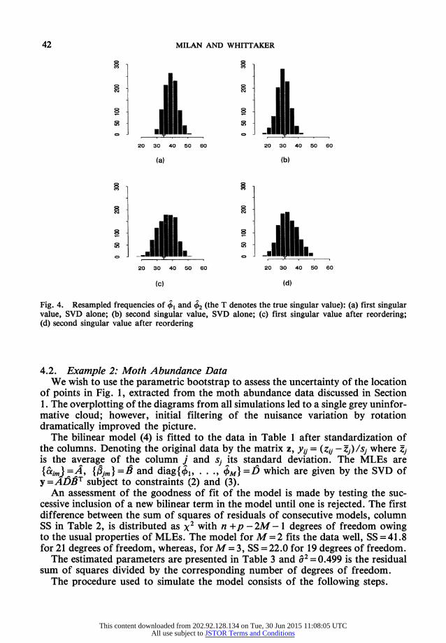
Estimates of the sampling densities can be obtained from the simulation with histograms or by using more advanced smoothing techniques. The histograms of Fig. 4 show the frequencies obtained after 1000 repetitions of the simulation process, Figs 4(a) and 4(b) using SVD alone and Figs 4(c) and 4(d) after reordering. These histograms demonstrate the effects of the imposed order on the singular values at constraint (3), with ?1 falling well above the true value of 4 = 34.4, indicated on the diagrams by the letter 'T'. There is also an indication of bias in the sampling distribution of /.2 but, after application of reordering, Figs 4(c) and 4(d) indicate some reduction at the cost of seeing the variance increase. These pictures illustrate the fact that the first sample eigenvalue is an overestimate of the corresponding population value; see Loh (1991) for a recent reference to this phenomenon.




20 30 40 50 60 20 30 40 50 60

(a) (b)

20 30 40 50 60 20 30 40 50 60

(c) (d)

Fig. 4. Resampled frequencies of +, and +2 (the T denotes the true singular value): (a) first singular value, SVD alone; (b) second singular value, SVD alone; (c) first singular value after reordering; (d) second singular value after reordering

4.2. Example 2: Moth Abundance Data We wish to use the parametric bootstrap to assess the uncertainty of the location

of points in Fig. 1, extracted from the moth abundance data discussed in Section 1. The overplotting of the diagrams from all simulations led to a single grey uninfor- mative cloud; however, initial filtering of the nuisance variation by rotation dramatically improved the picture.

The bilinear model (4) is fitted to the data in Table 1 after standardization of the columns. Denoting the original data by the matrix z, yij = (zij - Zj) Isj where -

is the average of the column j and sj its standard deviation. The MLEs are {&amJ=A9 {toIm}=B and diag{41, .. ., }=D which are given by the SVD of y=ADBT subject to constraints (2) and (3).

An assessment of the goodness of fit of the model is made by testing the suc- cessive inclusion of a new bilinear term in the model until one is rejected. The first difference between the sum of squares of residuals of consecutive models, column SS in Table 2, is distributed as x2 with n +p - 2M - 1 degrees of freedom owing to the usual properties of MLEs. The model for M = 2 fits the data well, SS = 41.8 for 21 degrees of freedom, whereas, for M = 3, SS = 22.0 for 19 degrees of freedom.

The estimated parameters are presented in Table 3 and a2 = 0.499 is the residual sum of squares divided by the corresponding number of degrees of freedom.

The procedure used to simulate the model consists of the following steps.




TABLE 2 Test statistics for example 2

M RSS Degrees of freedom SS Degrees of freedom

0 154.0 154 1 96.7 131 57.3 23 2 54.9 110 41.8 21 3 32.9 91 22.0 19

(a) Compute t =A2D2B2 with the A2, D2 and B2 given in Table 3. (b) Generate values of *J with distribution N(0, CJ2) and compute x tij= +

J. Compute z,J = (XJ- xJ*)/S . (c) Compute the sampled values A*, D2* and B* through the SVD of z* =

A*D2*(B2*)T and compute the values of the co-ordinates. The sequence of simulation (steps (b) and (c)) and rotation filtering (as described

in the previous section) is repeated 1000 times. The set of estimates from Table 3 is used as the 'true' value for simulation and also used as the reference set for the rotation filtering technique.

After rotation, approximate tolerance regions with 0.8 probability for each species in the diagram are constructed. A quick way of performing this task is to superimpose a 20 x 20 grid over the plot for each species separately, to count the frequencies on each cell of the grid, to select a level such that the sum of all frequencies above that level is approximately 80% of the total of simulations and finally to draw a contour at this level by using the 'contour' function available in the language S. The resulting plot is Fig. 5. An alternative way to draw these

TABLE 3 Estimated parameters for example 2

Parameter Values for the following values of m: Parameter Values for the following values of m: m=J m=2 m=J m=1

Okm 7.570 6.465 (g1m -0.078 0.309 atim 0.235 0.116 I2m -0.225 0.208 ct2m 0.039 0.645 I3m -0.289 0.082 Ct3m 0.110 -0.213 I4m -0.298 0.099 ct4m -0.348 0.048 I5m -0.317 0.175 ct5m -0.097 0.422 I6m -0.373 0.136 ci6m -0.358 -0.111 I7m -0.267 0.065 ct7m -0.199 -0.119 I8m -0.338 0.184 cx8m -0.272 -0.135 I9m -0.342 0.156 cxgm -0.182 -0.261 giom 0.242 0.419 otiOm 0.183 0.124 liim 0.270 0.370 ciilm 0.664 -0.055 I12m 0.133 0.282 a12m 0.227 -0.462 I13m 0.044 0.446

I14m 0.278 0.376




B

B

-4 -2 0 2 4 6

1 st principal coordinate

Fig. 5. Tolerance regions for example 2

regions would be to use convex hulls peeling, as described by Green and Silverman (1979). The 8007 value was found, after some experimentation, to give reasonable definition.

Fig. 5 shows polygons approximating the 800/ tolerance region for each point of the plot having filtered by rotation. (In fact, the probability of the region is greater than 0.80 since the nuisance variation is minimized but not eliminated.) The letter next to each polygon identifies the polygon and the letter inside the polygon is situated at the original estimate of the position of the point in the plot, obtained from Table 3.

These polygons show the pattern of abundance of each species distributed over the sites considered in this study. In this plot the larger the area of intersection of the polygons the greater is the similarity between the pattern of abundance of the corresponding species over the sites. The tolerance regions are generally circular though not all of the same size or shape. Furthermore the original estimates are not always at the centre of the polygon; see for instance B and K.

We can now give a substantive interpretation to Fig. 5. Species K is quite distinct from all the others. Species F, G, H and I present practically the same patterns and species D is very close to them forming a group, {F, G, H, I, D}. Similarly species A and J form the group {A, J} with the area occupied by species A practically inside the area occupied by J. J has the greatest variability of all species. Less clear is the group formed by L and C, and the group formed by B and E. Species C and L show a similar pattern with C closer to groups {F, G, H, I, D} and {A, J}. Species L is distinct from group {F, G, H, I, D} and with a small intersection with group




{A, J}. Species C has intersections with groups {F, G, H, I, D} and {A, J}. Species B and E display a similar pattern although B shows no similarity with group {F, G, H, I, D} whereas E, with larger area, is closer to group {F, G, H, I, D} than B is.

4.3. Example 3: Principal Components Analysis of Frets's Heads Data Example 3 illustrates the application of the techniques to the PCA of a variance

matrix. The data used here come from Mardia et al. (1979), p. 121. They consist of two measurements (head length and head breadth) on the first and second adult sons in a sample of 25 families, leading to a 25 x 4 data matrix z. As the measures are homogeneous it seems natural not to scale the data.

The data are modelled as 25 independent replicates from a multivariate normal distribution with arbitrary mean and variance-covariance matrix E. The MLEs are the sample mean and sample variance. The MLEs of the principal components can be obtained by an SVD of the data matrix or as an eigendecomposition of the sample variance matrix S. The parametric bootstrap repeatedly samples z4 = z + TE?' for i = 1, 2,..., 25, where each e* is a four-dimensional vector of independent standard normal deviates and TT' = S.

To assess the variability of the column points (the head measurements) in the two- dimensional display, rotation is applied to the first two dimensions of the SVD of y* where y" = z4 - z denotes the centred data. The results are displayed in Fig. 6. The reference points are the MLEs. The symmetries in the data (variables 1 and 3 are head length of the two sons; variables 2 and 4 are head breadths) are roughly preserved. The first dimension is heavily weighted towards lengths. The MLE for variable 1 is not at the centre of the tolerance region. Notably variable 2 has a larger region than variable 4 because it has a higher variability in the third and fourth dimensions, a fact that is not obvious in displays without tolerance regions.

0

0

-0.8 -0.6 -0.4 -0.2 0.0 1 st component

Fig. 6. Tolerance regions for example 3




Although the bilinear model in equation (4) provides the same MLEs of the point locations, which have the same interpretation as PCA, it is not an equivalent model and the parametric bootstrap gives different tolerance regions. The difference lies in the distribution of the residuals: in PCA the residuals are not independent. This affects the resampling distribution.

5. Discussion This paper has proposed a simple model-based simulation technique, the para-

metric bootstrap, to investigate the effect of sampling variation on estimates drawn from a model that incorporates an SVD. One detailed application assessed the marginal sampling distributions of the position of each point, and a second was to construct approximately unbiased intervals for a given singular value.

Because of the SVD some filtering of the estimates may be required. Rotation is the most general technique and provides the clearest graphics, although it is computationally more expensive. The value of these filtering techniques depends on the specific model generating the data: if the noise level is high then no amount of filtering will distinguish the points; if the noise level is low and the singular values are well separated then only reflection to overcome the arbitrary sign of the singular vectors is needed; however, if the noise level is low and the singular values are close then filtering is beneficial.

Several sources of uncertainty are inherent in statistical modelling and only that due to sampling variation from the true model is displayed in this approach. Nuisance variation is an artefact of the resampling and its effects are mitigated by filtering. Other sources might include stochastic variation of the parameters of the model, or a predictive uncertainty due to lack of model fit. Neither of these has been examined here.

The standard approach for evaluating sampling variation is to calculate asymptotic regions by inverting the information matrix derived from the model; see, for instance, Muirhead (1982), chapter 9, for PCA and Krzanowski (1989) in the context of CVA. However, the latter approach requires the group structure present in CVA. In addition, these regions are asymptotic and may substantially differ from resampled intervals in small samples, and also the constraints of the SVD make calculation of the appropriate region quite complicated, and conse- quently difficult to generalize to more elaborate models. Resampling is a relatively quick and simple solution.

The bootstrap suggested by Krzanowski and Radley (1989) for CVA resamples from just one group at a time, holding the observations in the other groups fixed. Supplementary points, used by Greenacre (1984) to assess random variation in correspondence analysis displays, can be described in the context of the bilinear model (4) above, and the method is also seen to adopt a form of partial resampling. Here, the fitted values from model (4) based on the original set of data are Y=ADBT and the row co-ordinates are AD ( = YB). For each resampled data set Y* the supplementary co-ordinates are taken from the rows of Y*B instead of Y*B* where B* denotes estimates from the bootstrap sample Y*.

This partial resampling is cheap as it eliminates the estimation step, involving one SVD, and does not use Procrustes analysis, so saving a further SVD. But because it does not repeat the estimation step it does not give a full simulation of the




sampling variation and the size of the region produced may be quite different from that obtained when using Y*B*. Although this form of partial resampling generates less nuisance variation, we would argue that it leads to inappropriate regions. The following argument suggests that the regions can be wrongly centred and too small.

Consider the simplest linear regression model yi =xi f + -i for i = 1, 2, .. ., n, with the xs fixed and known and {ei} independent N(O, a 2) random variables with a2 known. The least squares estimate of i3 is

n -1 n

Xi=l xi=l

and the raw residuals are ei =yi -9i where 9i =xxi. Suppose that a confidence interval for the mean of the observation at xr is to be computed from the parametric bootstrap. Full resampling repeatedly samples c", i = 1, 2, . . ., n, indepen- dently from N(O, (2), to compute y?* =. c + e, so that refitting gives

n \-1 n

and Yr* = Xr*. The required confidence interval is derived empirically from the set of bootstrap samples {Yr*}. The size of the interval can be derived by noting that with full resampling

Yr = Yr+Xr (ZEx) I XiEI

so that the error term from the bootstrap sample has variance a2xr (27= 1x?) -1, which accurately reflects the sampling variation in estimating the parameter ,3.

However, partial resampling holds all the yi fixed apart from Yr which is chosen as Yr +Er* where E* - N(O, a'). A little algebra shows that, after refitting, the partially resampled y is

Yr Y-r + Xr ( x2)E*

where the first term Y-r r -xr (NI= 1 xi2) - ler is an estimate of E(yr) based on the fitted value adjusted by the raw residual in the original sample. (It is not a deletion quantity as it depends in part on Yr.) Only the second term varies in repeated samples, and as can be seen has variance

&2X4 (Yx2 which is always smaller than the variance in full resampling.

In conclusion, although partial resampling may be appropriate for assessing outliers it does not completely allow for sampling variation in estimating the regression coefficient ,3.

The validation of the filtering techniques beyond the examples considered here requires further work. A reasonable way to conduct such an exercise is through experiments that evaluate the repeated sampling properties of filtering.




(a) Given a set of 'true values' of parameters, generate a large sample of matrix 'observations' by adding random error.

(b) Estimate the parameters and filter to obtain the tolerance regions. (c) Compare the frequency with which the region includes the true value with

the ostensible tolerance level. In the reordering technique it is possible that an inversion occurs between one

singular value in the model, qOfm, with m < M, and one not in the model, Om, with m > M. For instance, with a two-dimensional model, the first and third singular vectors in a simulation might correspond to the first and second in the reference. This extra source of variation may be filtered out by comparing all singular values rather than the first M.

The simple bilinear model with normally distributed errors extends without much difficulty to more general models. Suppose now that E(yij) =g(Oij, rij), where g is a suitable link function that includes bilinear terms Oij, and possibly other parameters such as a general mean and row and column effects denoted by Trj. The y,j are sampled from some distribution (e.g. normal, Poisson) with this mean. The bilinear term is expressed as

M

oij = Z /maimf3im. m=l

Examples of this general bilinear model are correspondence analysis, described in Greenacre (1984), the row-column (RC) association model and RC canonical correlation models as in Goodman (1985, 1986). Further constraints, such as those of the SVD, are necessary to make this model identifiable. The row co-ordinates are AD; the detailed interpretation of distances in the diagram depends on the function g.

Acknowledgements We are grateful to the referees for their comments which substantially helped to

improve the original draft of this paper. The research was completed while the first author was on leave of absence from Universidade Federal de Sao Carlos, Brazil, and was partially supported by CAPES/MEC (Brazil).

References

Becker, R. A., Chambers, J. M. and Wilks, A. R. (1988) The New S Language: a Programming Environment for Data Analysis and Graphics. Belmont: Wadsworth and Brooks/Cole.

Carlin, B. P. and Gelfand, A. E. (1991) A sample reuse method for accurate parametric empirical Bayes confidence intervals. J. R. Statist. Soc. B, 53, 189-200.

Digby, P.G. N. and Kempton, R. A. (1987) Multivariate Analysis of Ecological Communities. London: Chapman and Hall.

Efron, B. (1979) Bootstrap methods: another look at the jackknife. Ann. Statist., 7, 1-26. Gabriel, K. R. (1978) Least squares approximation of matrices by additive and multiplicative models.

J. R. Statist. Soc. B, 40, 186-196. Geyer, C. J. (1991) Constrained maximum likelihood exemplified by isotonic convex logistic regres-

sion. J. Am. Statist. Ass., 86, 717-724. Golub, G. N. and van Loan, C. F. (1989) Matrix Computations. Baltimore: Johns Hopkins University

Press.




Goodman, L.A. (1985) The analysis of cross-classified data having ordered and/or unordered categories: association models, correlation models, and asymmetry models for contingency tables with or without missing entries. Ann. Statist., 13, 10-69.

(1986) Some useful extensions of the usual correspondence analysis approach and the usual log-linear models approach in the analysis of contingency tables. Int. Statist. Rev., 54, 243-309.

Gower, J. C. (1966) Some distance properties of latent root and vector methods used in multivariate analysis. Biometrika, 53, 325-338.

(1971) Statistical methods of comparing different multivariate analyses of the same data. In Mathematics in the Archaeological and Historical Sciences (eds F. R. Hodson, D. G. Kendall and P. Tautu), pp. 138-149. Edinburgh: Edinburgh University Press.

Green, P. J. and Silverman, B. W. (1979) Constructing the convex hull of a set of points in the plane. Comput. J., 22, 262-266.

Greenacre, M. J. (1984) Theory and Applications of Correspondence Analysis. London: Academic Press.

Hinkley, D. V. (1988) Bootstrap methods. J. R. Statist. Soc. B, 50, 321-337. Krzanowski, W. J. (1988) Principles of Multivariate Analysis: a User's Perspective. Oxford: Oxford

University Press. (1989) On confidence regions in canonical variate analysis. Biometrika, 76, 107-116.

Krzanowski, W. J. and Radley, D. (1989) Nonparametric confidence and tolerance regions in canonical variate analysis. Biometrics, 45, 1163-1173.

Loh, W.-L. (1991) Estimating covariance matrices. Ann. Statist., 19, 283-296. Mardia, K. V., Kent, J. T. and Bibby, J. M. (1979) Multivariate Analysis. London: Academic Press. Muirhead, R. J. (1982) Aspects of Multivariate Statistical Theory. New York: Wiley. Ringrose, T. J. (1992) Bootstrapping and correspondence analysis in archaeology. J. Arch. Sci., 19,

615-629. Ringrose, T. J. and Krzanowski, W. J. (1991) Simulation study of confidence regions for canonical

variate analysis. Statist. Comput., 1, 41-46. Schott, J. R. (1990) Canonical mean projections and confidence regions in canonical variate analysis.

Biometrika, 77, 587-596. Sibson, R. (1978) Studies in the robustness of multidimensional scaling: Procrustes statistics. J. R.

Statist. Soc. B, 40, 234-238. Stewart, G. W. (1973) Introduction to Matrix Computations. New York: Academic Press.



application of the parametric bootstrap to models that...

Documents