introduction to correlation analysis and simple...
TRANSCRIPT
Introduction to Correlation Analysis
and Simple Linear Regression
1
Josefina V. Almeda
Stat 115
2014
Goals
After this, you should be able to:
• Calculate and interpret the simple correlation
between two variables
• Determine whether the correlation is significant
• Calculate and interpret the simple linear
regression equation for a set of data
• Understand the assumptions behind
regression analysis
• Determine whether a regression model is
significant 2
Goals
After this, you should be able to:
• Calculate and interpret confidence intervals for the regression coefficients
• Recognize regression analysis applications for purposes of prediction and description
• Recognize some potential problems if regression analysis is used incorrectly
• Recognize nonlinear relationships between two variables
(continued)
3
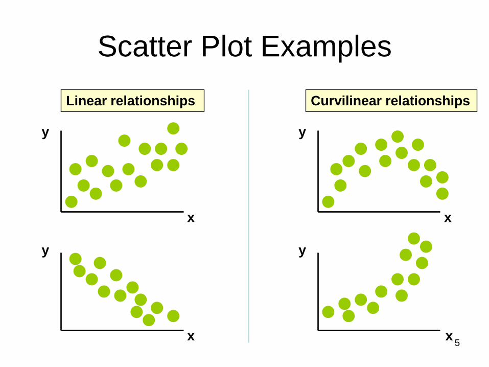
Scatter Plots and Correlation
• A scatter plot (or scatter diagram) is used
to show the relationship between two
variables
• Correlation analysis is used to measure
strength of the association (linear
relationship) between two variables
–Only concerned with strength of the
relationship
–No causal effect is implied
4
Scatter Plot Examples
y
x
y
x
y
y
x
x
Linear relationships Curvilinear relationships
5
Scatter Plot Examples
y
x
y
x
y
y
x
x
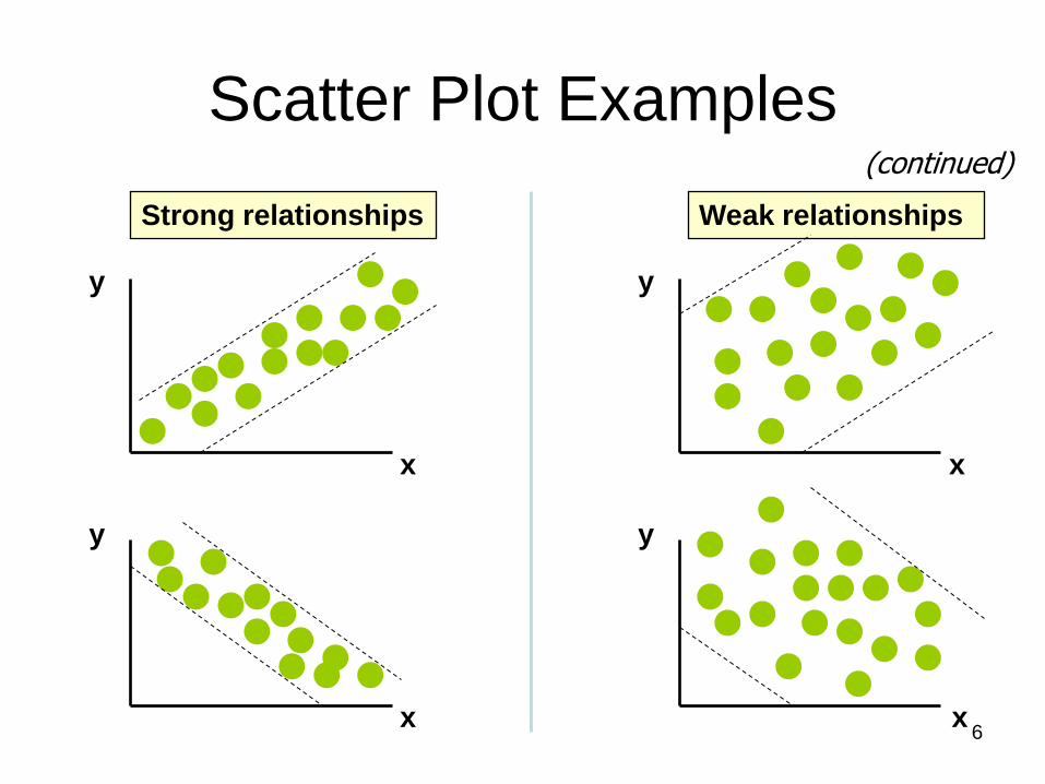
Strong relationships Weak relationships
(continued)
6
Scatter Plot Examples
y
x
y
x
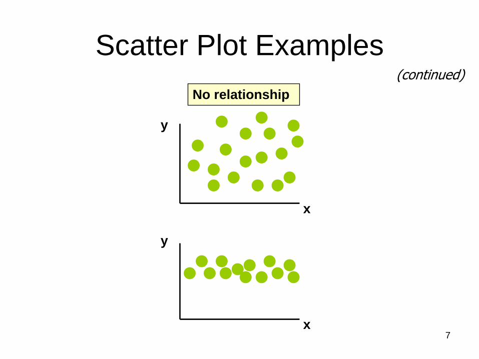
No relationship
(continued)
7
Correlation Coefficient
• The population correlation coefficient
ρ (rho) measures the strength of the
association between the variables
• The sample correlation coefficient r is
an estimate of ρ and is used to
measure the strength of the linear
relationship in the sample
observations
(continued)
8

Features of ρ and r
• Unit free
• Range between -1 and 1
• The closer to -1, the stronger the
negative linear relationship
• The closer to 1, the stronger the positive
linear relationship
• The closer to 0, the weaker the linear
relationship
9
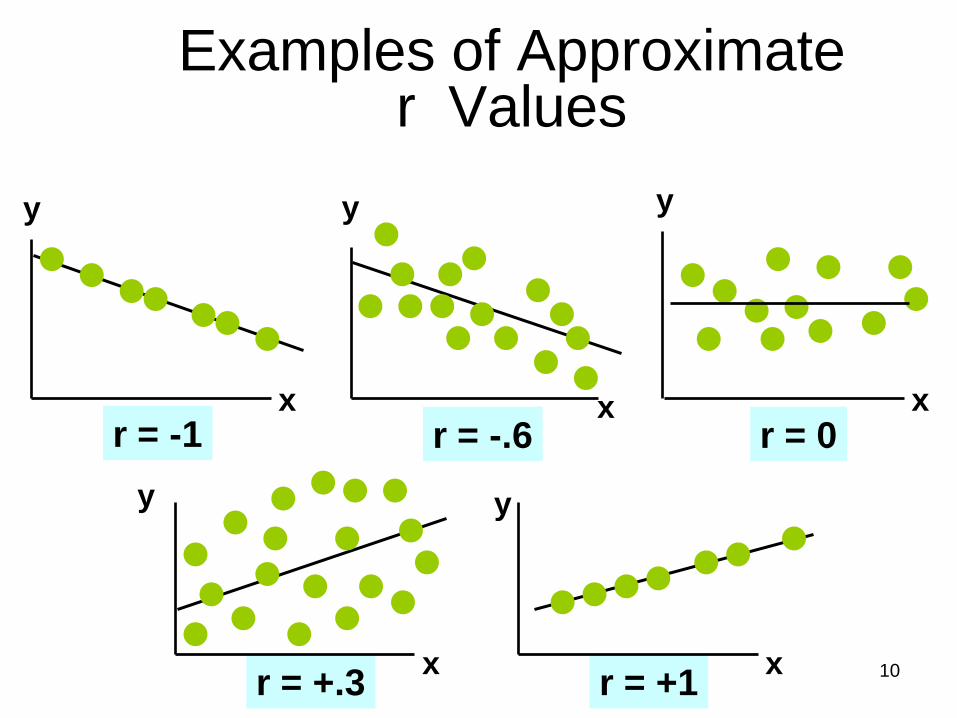
r = +.3 r = +1
Examples of Approximate r Values
y
x
y
x
y
x
y
x
y
x
r = -1 r = -.6 r = 0
10
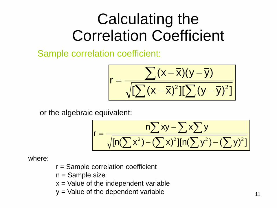
Calculating the Correlation Coefficient
])yy(][)xx([
)yy)(xx(r
22
where:
r = Sample correlation coefficient
n = Sample size
x = Value of the independent variable
y = Value of the dependent variable
])y()y(n][)x()x(n[
yxxynr
2222
Sample correlation coefficient:
or the algebraic equivalent:
11

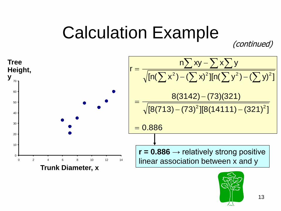
Calculation Example
Tree
Height
Trunk
Diamete
r
y x xy y2 x2
35 8 280 1225 64
49 9 441 2401 81
27 7 189 729 49
33 6 198 1089 36
60 13 780 3600 169
21 7 147 441 49
45 11 495 2025 121
51 12 612 2601 144
=321 =73 =3142 =14111 =713 12
0
10
20
30
40
50
60
70
0 2 4 6 8 10 12 14
0.886
](321)][8(14111)(73)[8(713)
(73)(321)8(3142)
]y)()y][n(x)()x[n(
yxxynr
22
2222
Trunk Diameter, x
Tree Height, y
Calculation Example (continued)
r = 0.886 → relatively strong positive
linear association between x and y
13
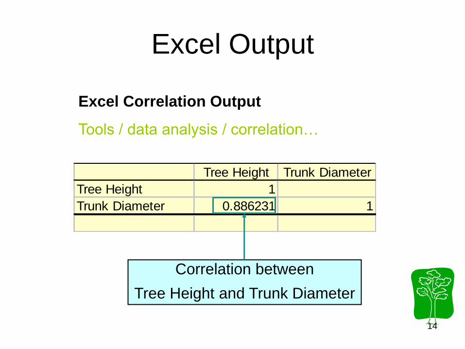
Excel Output
Tree Height Trunk Diameter
Tree Height 1
Trunk Diameter 0.886231 1
Excel Correlation Output
Tools / data analysis / correlation…
Correlation between
Tree Height and Trunk Diameter
14
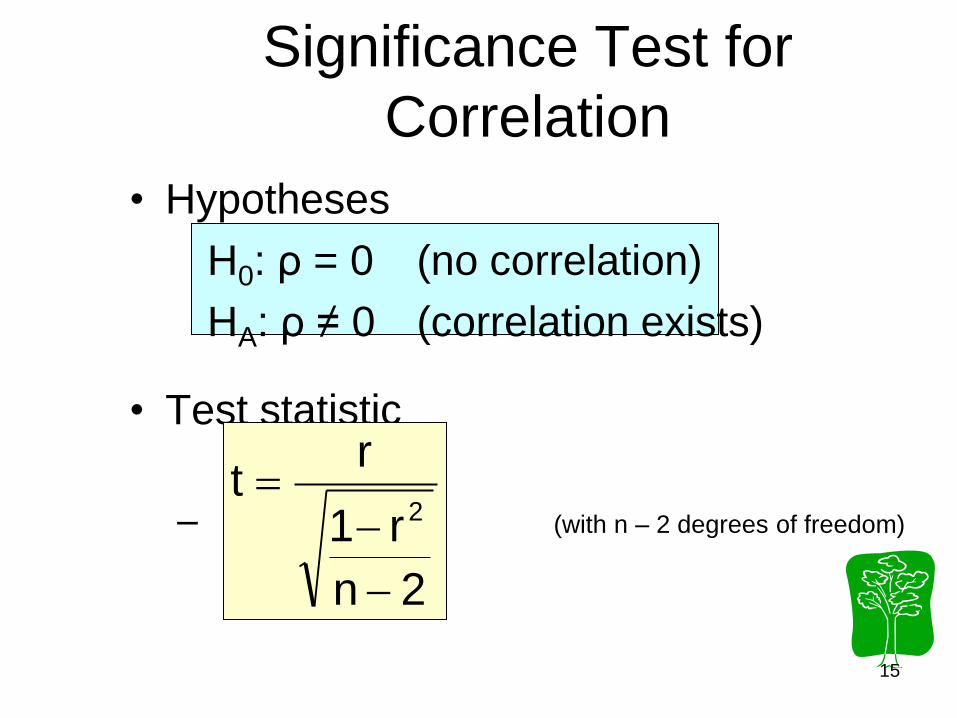
Significance Test for
Correlation
• Hypotheses
H0: ρ = 0 (no correlation)
HA: ρ ≠ 0 (correlation exists)
• Test statistic
– (with n – 2 degrees of freedom)
2n
r1
rt
2
15
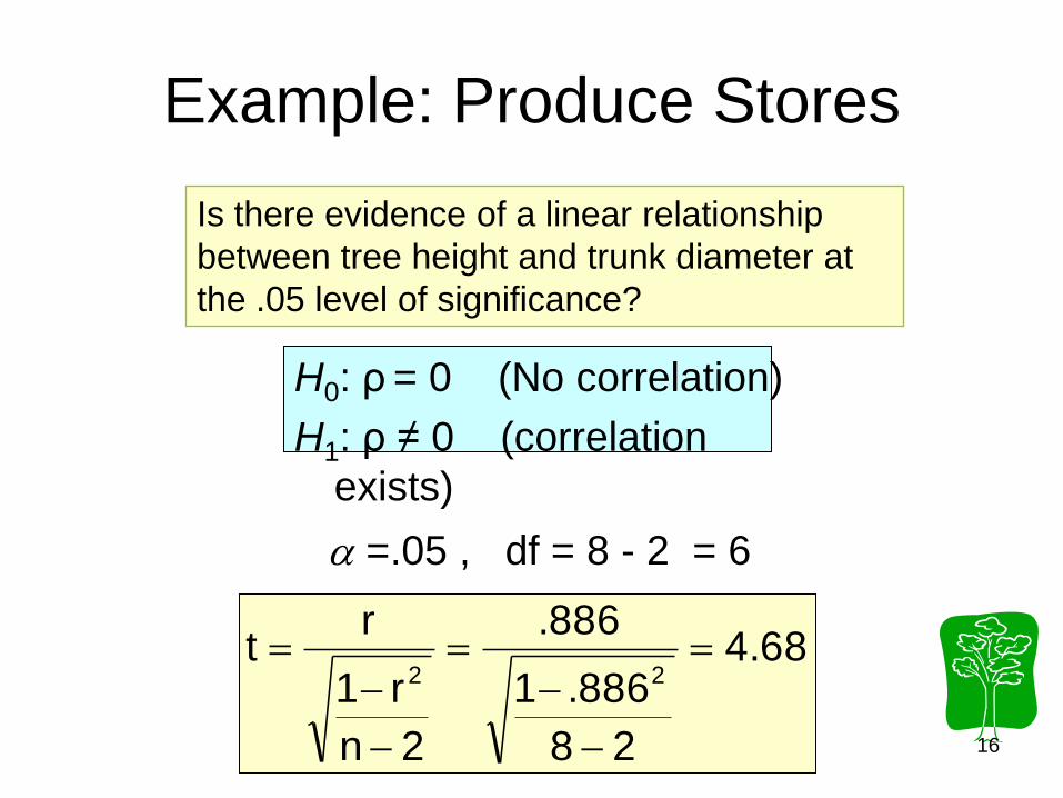
Example: Produce Stores
Is there evidence of a linear relationship
between tree height and trunk diameter at
the .05 level of significance?
H0: ρ = 0 (No correlation)
H1: ρ ≠ 0 (correlation
exists)
=.05 , df = 8 - 2 = 6
4.68
28
.8861
.886
2n
r1
rt
22
16
4.68
28
.8861
.886
2n
r1
rt
22
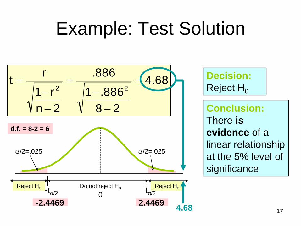
Example: Test Solution
Conclusion:
There is
evidence of a
linear relationship
at the 5% level of
significance
Decision:
Reject H0
Reject H0 Reject H0
/2=.025
-tα/2
Do not reject H0
0
tα/2
/2=.025
-2.4469 2.4469 4.68
d.f. = 8-2 = 6
17

Introduction to Regression Analysis
• Regression analysis is used to:
– Predict the value of a dependent variable
based on the value of at least one
independent variable
– Explain the impact of changes in an
independent variable on the dependent
variable
Dependent variable: the variable we
wish to explain
Independent variable: the variable used
to explain the dependent variable 18
Simple Linear Regression
Model
• Only one independent variable, x
• Relationship between x and y is
described by a linear function
• Changes in y are assumed to be
caused by changes in x
19
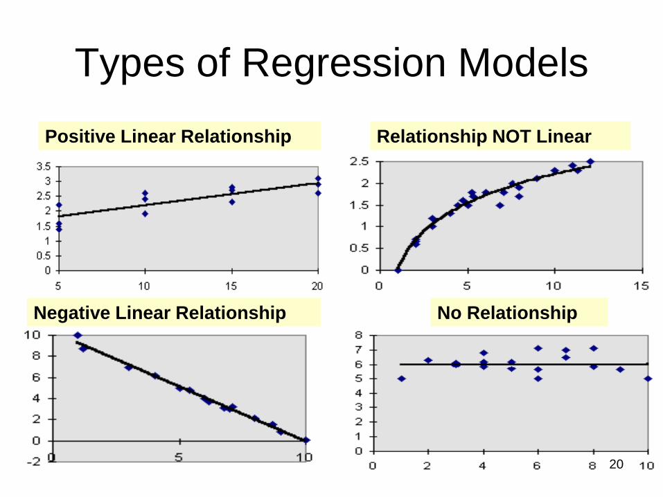
Types of Regression Models
Positive Linear Relationship
Negative Linear Relationship
Relationship NOT Linear
No Relationship
20

εxββy 10 Linear component
Population Linear Regression
The population regression model:
Population
y intercept
Population
Slope
Coefficient
Random
Error
term, or
residual Dependent
Variable
Independent
Variable
Random Error
component
21
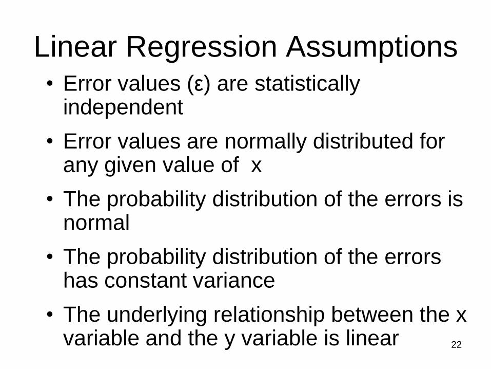
Linear Regression Assumptions • Error values (ε) are statistically
independent
• Error values are normally distributed for any given value of x
• The probability distribution of the errors is normal
• The probability distribution of the errors has constant variance
• The underlying relationship between the x variable and the y variable is linear 22
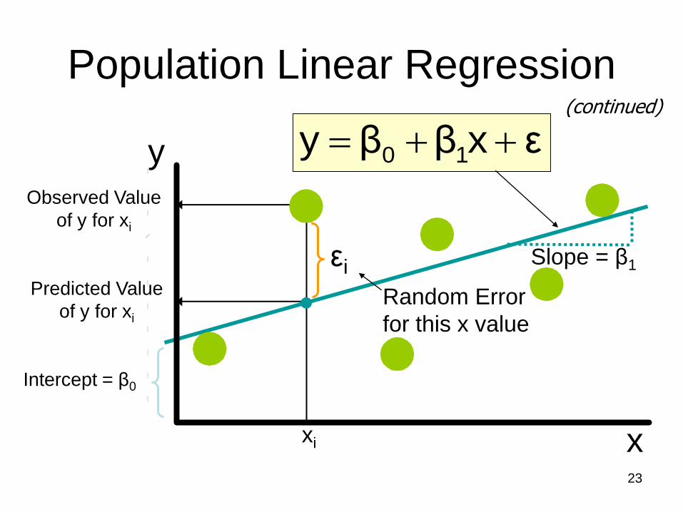
Population Linear Regression (continued)
Random Error
for this x value
y
x
Observed Value
of y for xi
Predicted Value
of y for xi
εxββy 10
xi
Slope = β1
Intercept = β0
εi
23

xbby 10i
The sample regression line provides an estimate of
the population regression line
Estimated Regression Model
Estimate of
the regression
intercept
Estimate of the
regression slope
Estimated
(or predicted)
y value
Independent
variable
The individual random error terms ei have a mean of zero
24

Least Squares Criterion
• b0 and b1 are obtained by finding the
values of b0 and b1 that minimize the
sum of the squared residuals
2
10
22
x))b(b(y
)y(ye
25
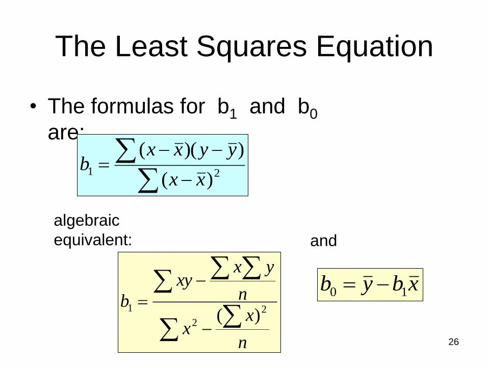
The Least Squares Equation
• The formulas for b1 and b0
are:
algebraic
equivalent:
n
xx
n
yxxy
b2
2
1)(
21)(
))((
xx
yyxxb
xbyb 10
and
26
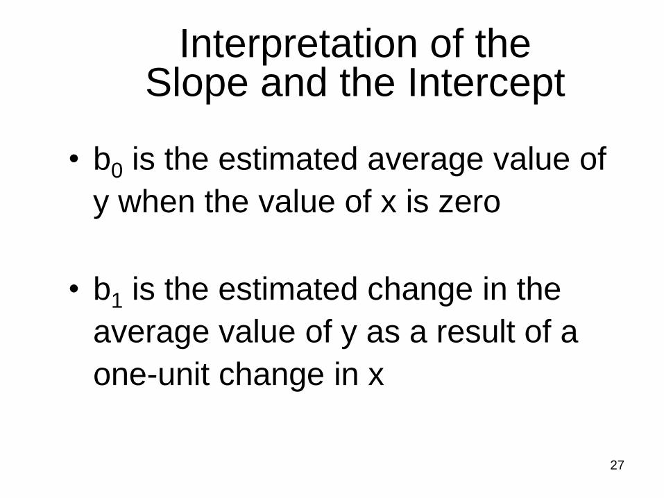
• b0 is the estimated average value of
y when the value of x is zero
• b1 is the estimated change in the
average value of y as a result of a
one-unit change in x
Interpretation of the Slope and the Intercept
27
Finding the Least Squares
Equation
• The coefficients b0 and b1 will
usually be found using computer
software, such as Excel or Minitab
• Other regression measures will also
be computed as part of computer-
based regression analysis
28
Simple Linear Regression Example
• A real estate agent wishes to examine the
relationship between the selling price of a
home and its size (measured in square
feet)
• A random sample of 10 houses is selected
–Dependent variable (y) = house price in
$1000s
– Independent variable (x) = square feet
29
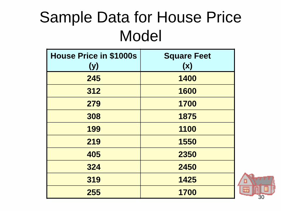
Sample Data for House Price
Model House Price in $1000s
(y)
Square Feet
(x)
245 1400
312 1600
279 1700
308 1875
199 1100
219 1550
405 2350
324 2450
319 1425
255 1700 30
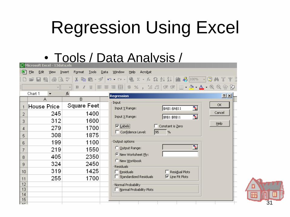
Regression Using Excel
• Tools / Data Analysis /
Regression
31
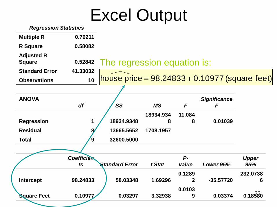
Excel Output Regression Statistics
Multiple R 0.76211
R Square 0.58082
Adjusted R
Square 0.52842
Standard Error 41.33032
Observations 10
ANOVA df SS MS F
Significance
F
Regression 1 18934.9348
18934.934
8
11.084
8 0.01039
Residual 8 13665.5652 1708.1957
Total 9 32600.5000
Coefficien
ts Standard Error t Stat
P-
value Lower 95%
Upper
95%
Intercept 98.24833 58.03348 1.69296
0.1289
2 -35.57720
232.0738
6
Square Feet 0.10977 0.03297 3.32938
0.0103
9 0.03374 0.18580
The regression equation is:
feet) (square 0.10977 98.24833 price house
32
0
50
100
150
200
250
300
350
400
450
0 500 1000 1500 2000 2500 3000
Square Feet
Ho
use P
rice (
$1000s)
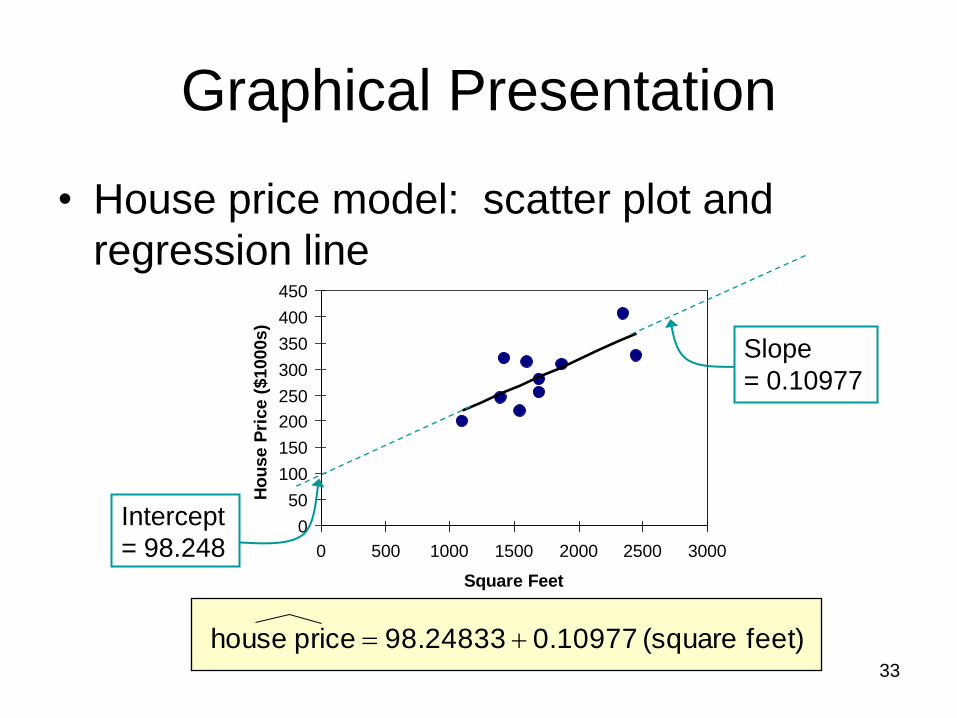
Graphical Presentation
• House price model: scatter plot and
regression line
feet) (square 0.10977 98.24833 price house
Slope
= 0.10977
Intercept
= 98.248
33
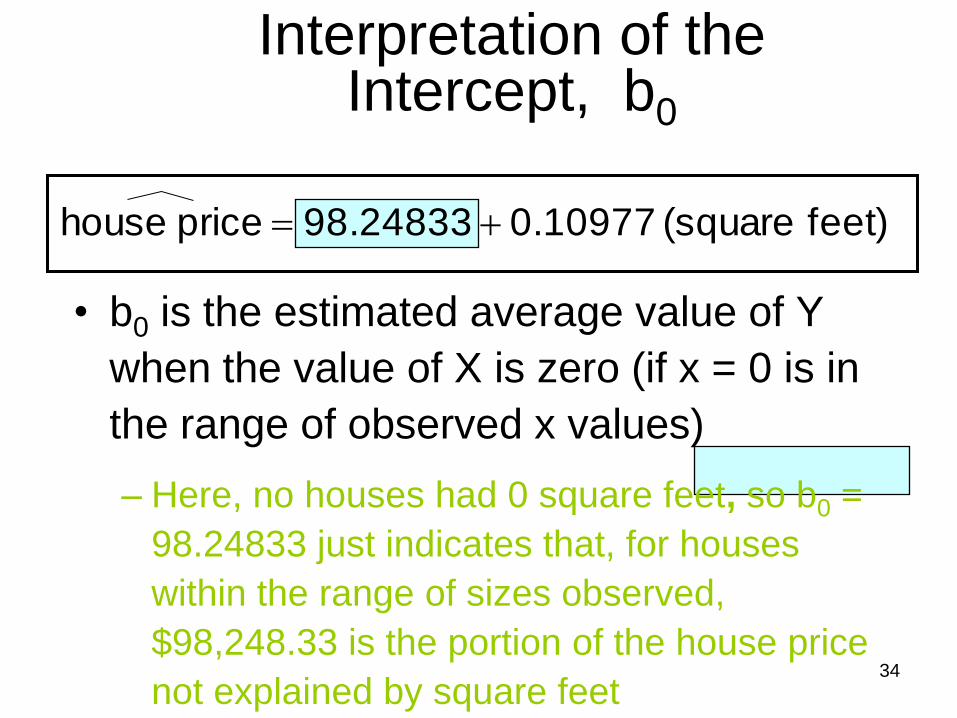
Interpretation of the Intercept, b0
• b0 is the estimated average value of Y
when the value of X is zero (if x = 0 is in
the range of observed x values)
– Here, no houses had 0 square feet, so b0 =
98.24833 just indicates that, for houses
within the range of sizes observed,
$98,248.33 is the portion of the house price
not explained by square feet
feet) (square 0.10977 98.24833 price house
34
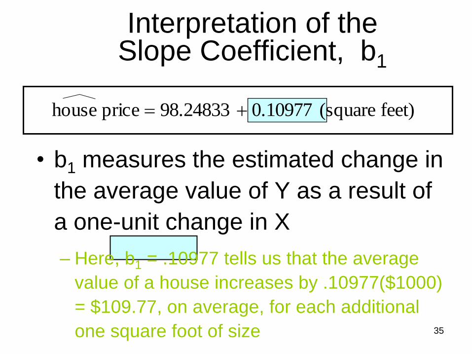
Interpretation of the Slope Coefficient, b1
• b1 measures the estimated change in
the average value of Y as a result of
a one-unit change in X
– Here, b1 = .10977 tells us that the average
value of a house increases by .10977($1000)
= $109.77, on average, for each additional
one square foot of size
feet) (square 0.10977 98.24833 price house
35

Least Squares Regression Properties
• The sum of the residuals from the least
squares regression line is 0 ( )
• The sum of the squared residuals is a
minimum (minimized )
• The simple regression line always passes
through the mean of the y variable and the
mean of the x variable
• The least squares coefficients are unbiased
estimates of β0 and β1
0)ˆ( yy
2)ˆ( yy
36

Explained and Unexplained
Variation
• Total variation is made up of two parts:
SSR SSE SST Total sum
of Squares
Sum of
Squares
Regression
Sum of
Squares Error
2)yy(SST 2)yy(SSE 2)yy(SSR
where:
= Average value of the dependent variable
y = Observed values of the dependent variable
= Estimated value of y for the given x value y
y
37
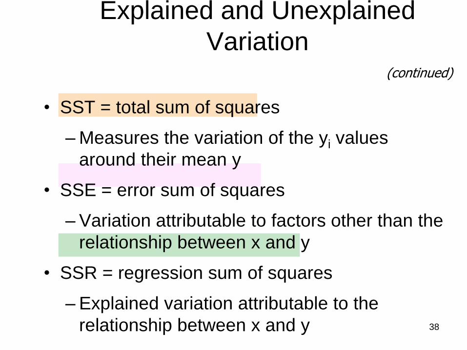
• SST = total sum of squares
– Measures the variation of the yi values
around their mean y
• SSE = error sum of squares
– Variation attributable to factors other than the
relationship between x and y
• SSR = regression sum of squares
– Explained variation attributable to the
relationship between x and y
(continued)
Explained and Unexplained
Variation
38
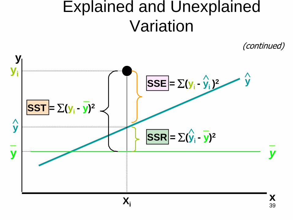
(continued)
Xi
y
x
yi
SST = (yi - y)2
SSE = (yi - yi )2
SSR = (yi - y)2
_
_
_
Explained and Unexplained
Variation
y
y
y _
y
39
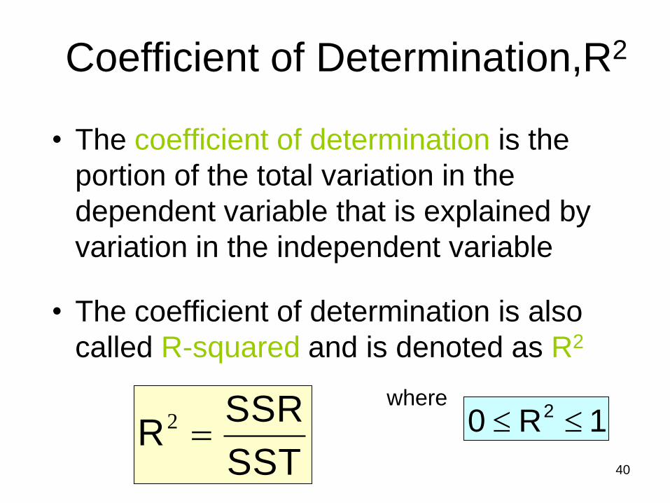
• The coefficient of determination is the
portion of the total variation in the
dependent variable that is explained by
variation in the independent variable
• The coefficient of determination is also
called R-squared and is denoted as R2
Coefficient of Determination,R2
SST
SSRR 2 1R0 2
where
40
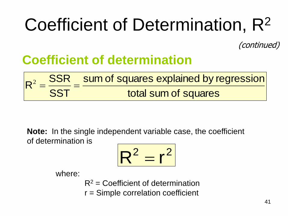
Coefficient of determination
Coefficient of Determination, R2
squares of sum total
regressionby explained squares of sum
SST
SSRR 2
(continued)
Note: In the single independent variable case, the coefficient
of determination is
where:
R2 = Coefficient of determination
r = Simple correlation coefficient
22 rR
41

R2 = +1
Examples of Approximate R2 Values
y
x
y
x
R2 = 1
R2 = 1
Perfect linear relationship
between x and y:
100% of the variation in y is
explained by variation in x
42
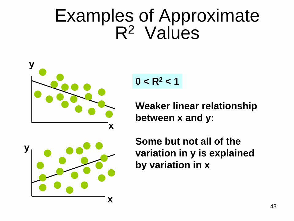
Examples of Approximate R2 Values
y
x
y
x
0 < R2 < 1
Weaker linear relationship
between x and y:
Some but not all of the
variation in y is explained
by variation in x
43
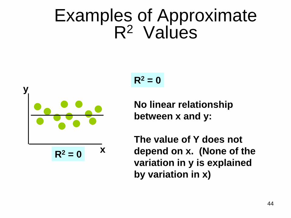
Examples of Approximate R2 Values
R2 = 0
No linear relationship
between x and y:
The value of Y does not
depend on x. (None of the
variation in y is explained
by variation in x)
y
x R2 = 0
44
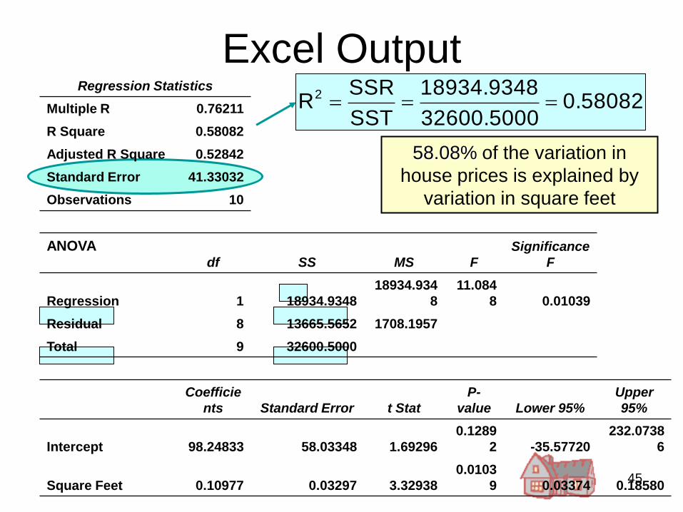
Excel Output Regression Statistics
Multiple R 0.76211
R Square 0.58082
Adjusted R Square 0.52842
Standard Error 41.33032
Observations 10
ANOVA df SS MS F
Significance
F
Regression 1 18934.9348
18934.934
8
11.084
8 0.01039
Residual 8 13665.5652 1708.1957
Total 9 32600.5000
Coefficie
nts Standard Error t Stat
P-
value Lower 95%
Upper
95%
Intercept 98.24833 58.03348 1.69296
0.1289
2 -35.57720
232.0738
6
Square Feet 0.10977 0.03297 3.32938
0.0103
9 0.03374 0.18580
58.08% of the variation in
house prices is explained by
variation in square feet
0.5808232600.5000
18934.9348
SST
SSRR2
45
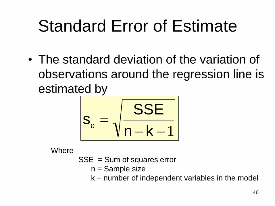
Standard Error of Estimate
• The standard deviation of the variation of
observations around the regression line is
estimated by
1
kn
SSEs
Where
SSE = Sum of squares error
n = Sample size
k = number of independent variables in the model
46
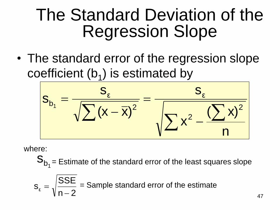
The Standard Deviation of the Regression Slope
• The standard error of the regression slope
coefficient (b1) is estimated by
n
x)(x
s
)x(x
ss
2
2
ε
2
εb1
where:
= Estimate of the standard error of the least squares slope
= Sample standard error of the estimate
1bs
2n
SSEsε
47
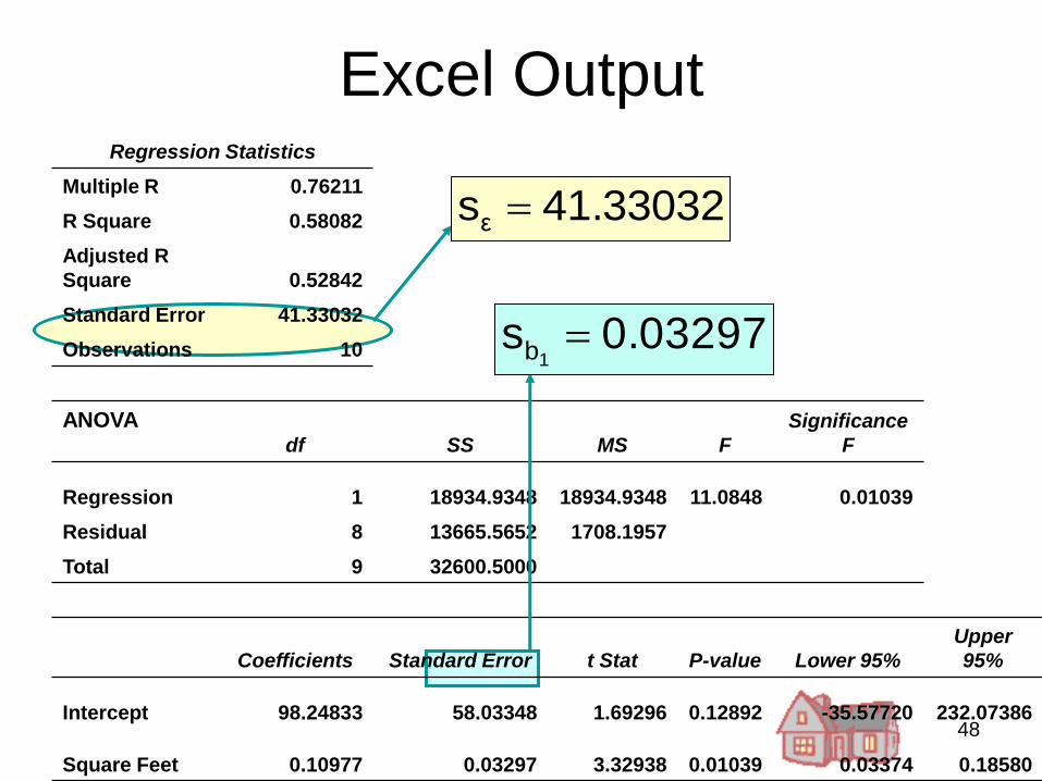
Excel Output Regression Statistics
Multiple R 0.76211
R Square 0.58082
Adjusted R
Square 0.52842
Standard Error 41.33032
Observations 10
ANOVA df SS MS F
Significance
F
Regression 1 18934.9348 18934.9348 11.0848 0.01039
Residual 8 13665.5652 1708.1957
Total 9 32600.5000
Coefficients Standard Error t Stat P-value Lower 95%
Upper
95%
Intercept 98.24833 58.03348 1.69296 0.12892 -35.57720 232.07386
Square Feet 0.10977 0.03297 3.32938 0.01039 0.03374 0.18580
41.33032sε
0.03297s1b
48
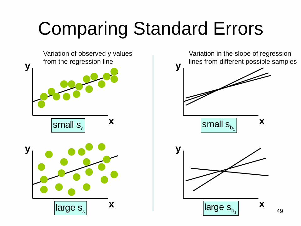
Comparing Standard Errors
y
y y
x
x
x
y
x
1bs small
1bs large
s small
s large
Variation of observed y values
from the regression line
Variation in the slope of regression
lines from different possible samples
49
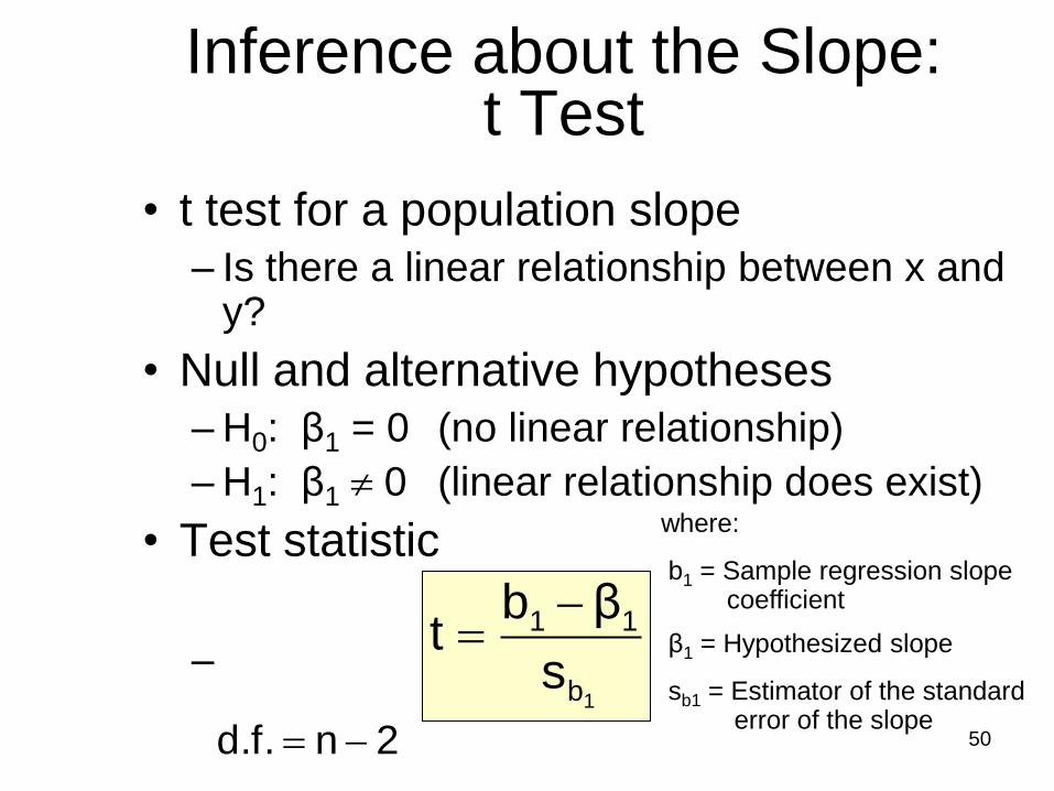
Inference about the Slope: t Test
• t test for a population slope
– Is there a linear relationship between x and y?
• Null and alternative hypotheses
– H0: β1 = 0 (no linear relationship)
– H1: β1 0 (linear relationship does exist)
• Test statistic
–
–
1b
11
s
βbt
2nd.f.
where:
b1 = Sample regression slope coefficient
β1 = Hypothesized slope
sb1 = Estimator of the standard error of the slope
50
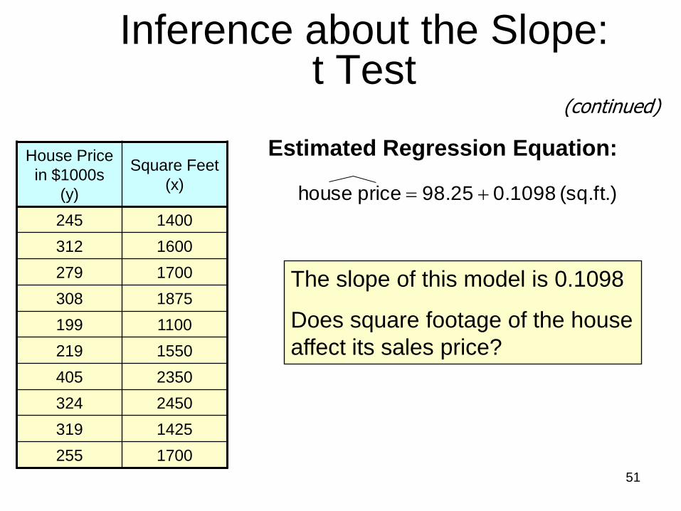
House Price
in $1000s
(y)
Square Feet
(x)
245 1400
312 1600
279 1700
308 1875
199 1100
219 1550
405 2350
324 2450
319 1425
255 1700
(sq.ft.) 0.1098 98.25 price house
Estimated Regression Equation:
The slope of this model is 0.1098
Does square footage of the house
affect its sales price?
Inference about the Slope: t Test
(continued)
51

Inferences about the Slope: t Test Example
H0: β1 = 0
HA: β1 0
Test Statistic: t = 3.329
There is sufficient evidence that
square footage affects house
price
From Excel output:
Reject H0
Coefficients
Standard
Error t Stat
P-
value
Intercept 98.24833 58.03348 1.69296
0.1289
2
Square
Feet 0.10977 0.03297 3.32938
0.0103
9
1bs t b1
Decision:
Conclusion: Reject H0 Reject H0
/2=.025
-tα/2
Do not reject H0
0
tα/2
/2=.025
-2.3060 2.3060 3.329
d.f. = 10-2 = 8
52
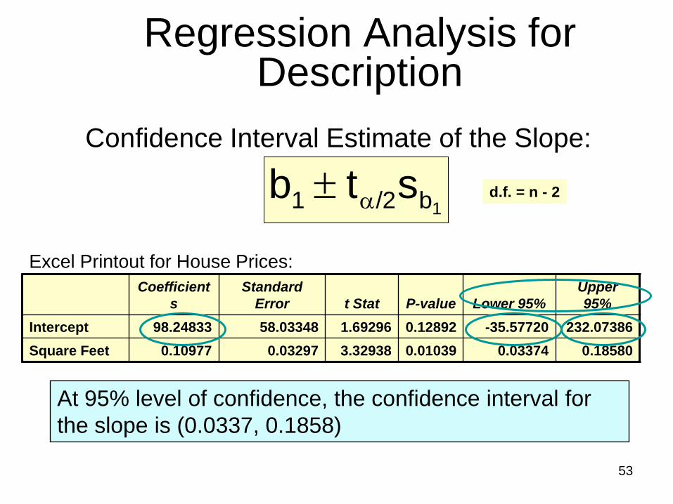
Regression Analysis for Description
Confidence Interval Estimate of the Slope:
Excel Printout for House Prices:
At 95% level of confidence, the confidence interval for
the slope is (0.0337, 0.1858)
1b/21 stb
Coefficient
s
Standard
Error t Stat P-value Lower 95%
Upper
95%
Intercept 98.24833 58.03348 1.69296 0.12892 -35.57720 232.07386
Square Feet 0.10977 0.03297 3.32938 0.01039 0.03374 0.18580
d.f. = n - 2
53
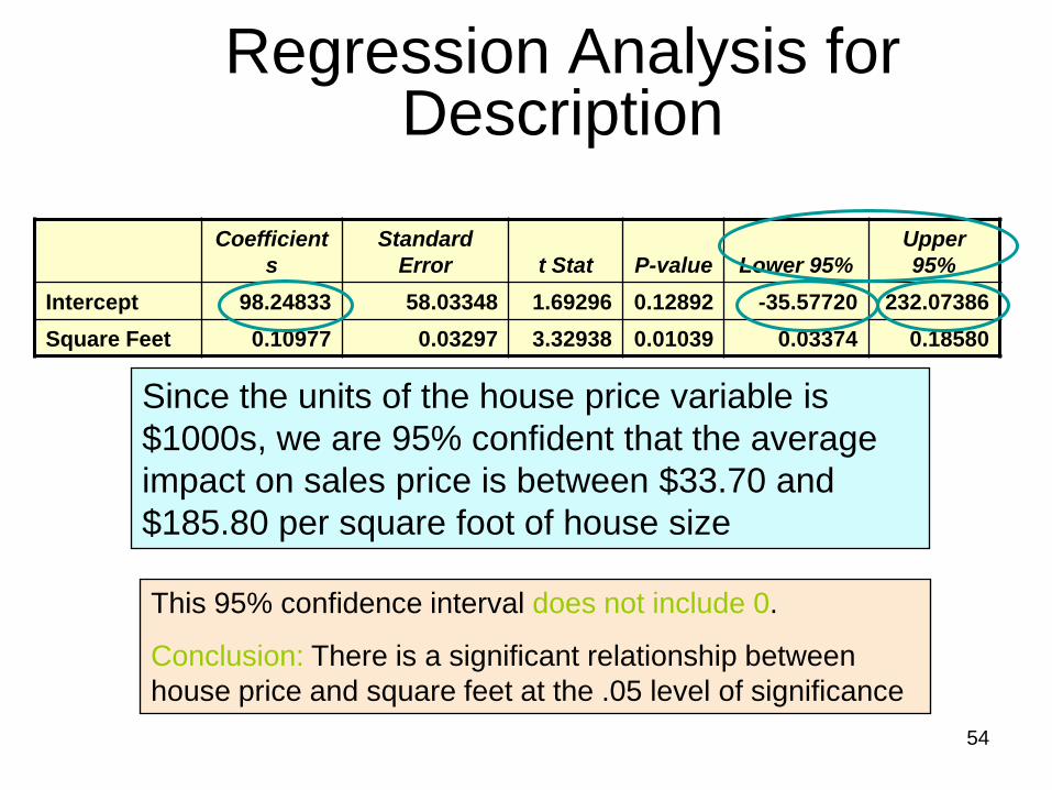
Regression Analysis for Description
Since the units of the house price variable is
$1000s, we are 95% confident that the average
impact on sales price is between $33.70 and
$185.80 per square foot of house size
Coefficient
s
Standard
Error t Stat P-value Lower 95%
Upper
95%
Intercept 98.24833 58.03348 1.69296 0.12892 -35.57720 232.07386
Square Feet 0.10977 0.03297 3.32938 0.01039 0.03374 0.18580
This 95% confidence interval does not include 0.
Conclusion: There is a significant relationship between
house price and square feet at the .05 level of significance
54
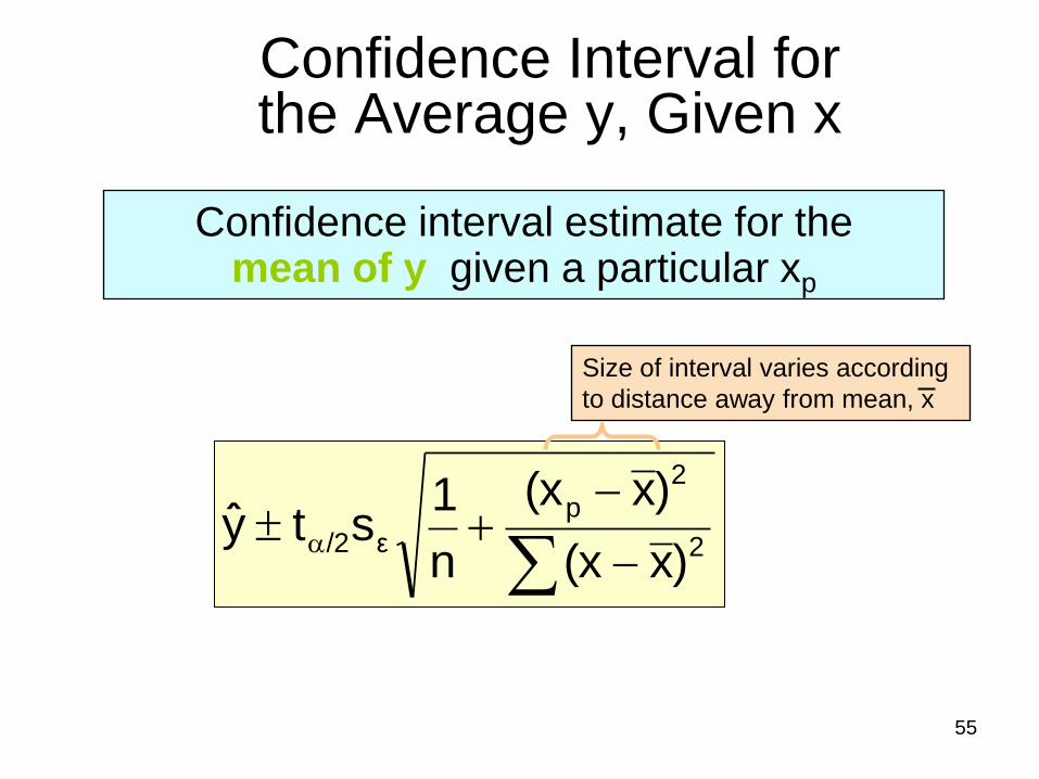
Confidence Interval for the Average y, Given x
Confidence interval estimate for the mean of y given a particular xp
Size of interval varies according
to distance away from mean, x
2
2
p
ε/2)x(x
)x(x
n
1sty
55
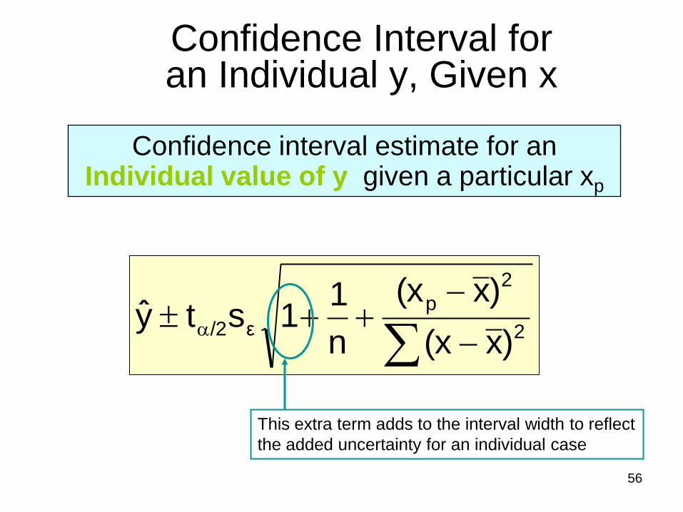
Confidence Interval for an Individual y, Given x
Confidence interval estimate for an Individual value of y given a particular xp
2
2
p
ε/2)x(x
)x(x
n
11sty
This extra term adds to the interval width to reflect
the added uncertainty for an individual case
56
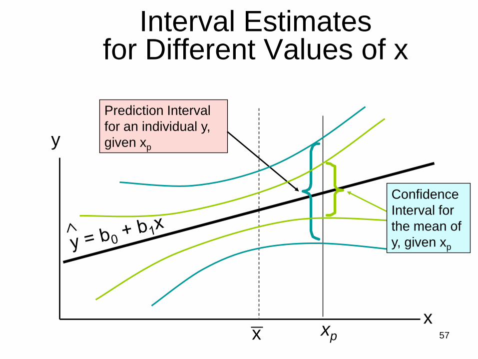
Interval Estimates for Different Values of x
y
x
Prediction Interval
for an individual y,
given xp
xp x
Confidence
Interval for
the mean of
y, given xp
57
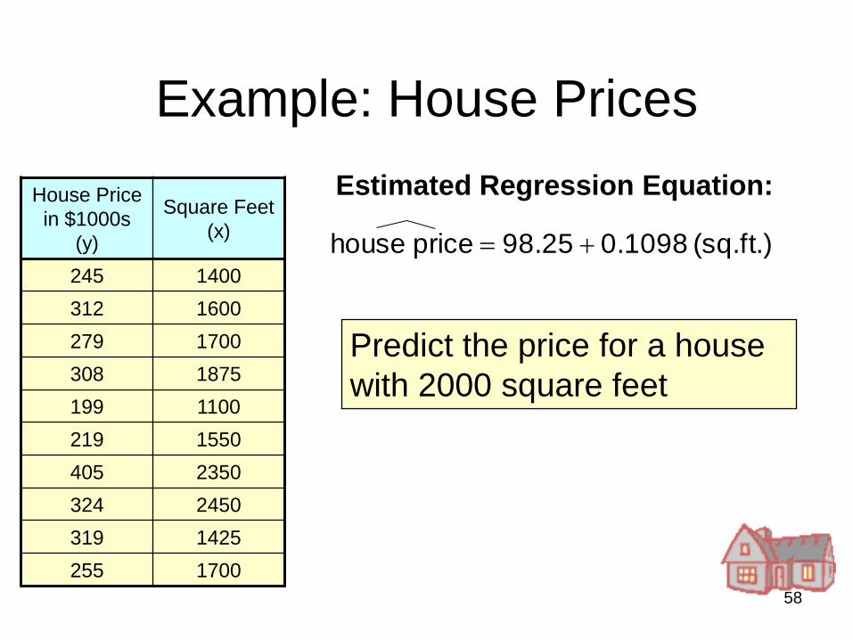
House Price
in $1000s
(y)
Square Feet
(x)
245 1400
312 1600
279 1700
308 1875
199 1100
219 1550
405 2350
324 2450
319 1425
255 1700
(sq.ft.) 0.1098 98.25 price house
Estimated Regression Equation:
Example: House Prices
Predict the price for a house
with 2000 square feet
58
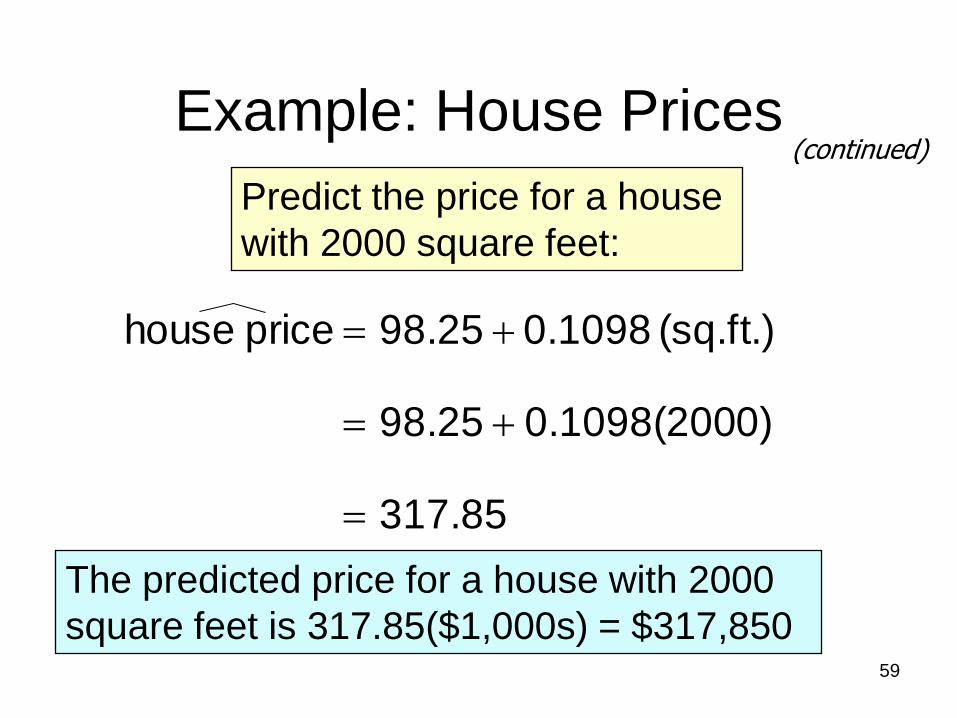
317.85
0)0.1098(200 98.25
(sq.ft.) 0.1098 98.25 price house
Example: House Prices
Predict the price for a house
with 2000 square feet:
The predicted price for a house with 2000
square feet is 317.85($1,000s) = $317,850
(continued)
59
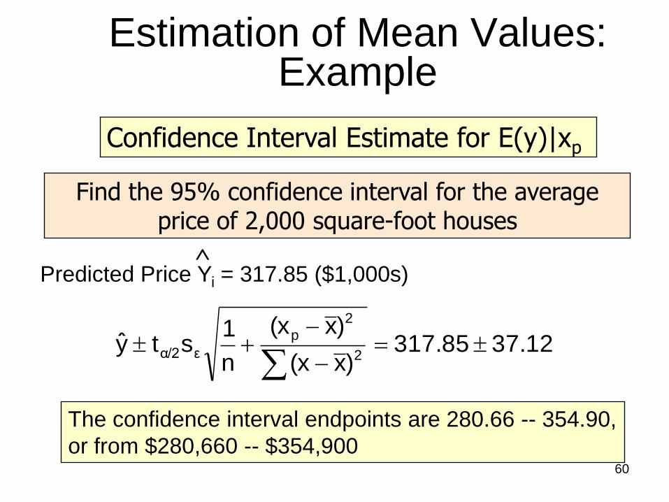
Estimation of Mean Values: Example
Find the 95% confidence interval for the average price of 2,000 square-foot houses
Predicted Price Yi = 317.85 ($1,000s)
Confidence Interval Estimate for E(y)|xp
37.12317.85)x(x
)x(x
n
1sty
2
2
p
εα/2
The confidence interval endpoints are 280.66 -- 354.90,
or from $280,660 -- $354,900 60
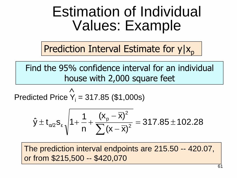
Estimation of Individual Values: Example
Find the 95% confidence interval for an individual house with 2,000 square feet
Predicted Price Yi = 317.85 ($1,000s)
Prediction Interval Estimate for y|xp
102.28317.85)x(x
)x(x
n
11sty
2
2
p
εα/2
The prediction interval endpoints are 215.50 -- 420.07,
or from $215,500 -- $420,070 61
Residual Analysis
• Purposes
–Examine for linearity assumption
–Examine for constant variance for all levels of x
–Evaluate normal distribution assumption
• Graphical Analysis of Residuals
–Can plot residuals vs. x
–Can create histogram of residuals to check for normality 62
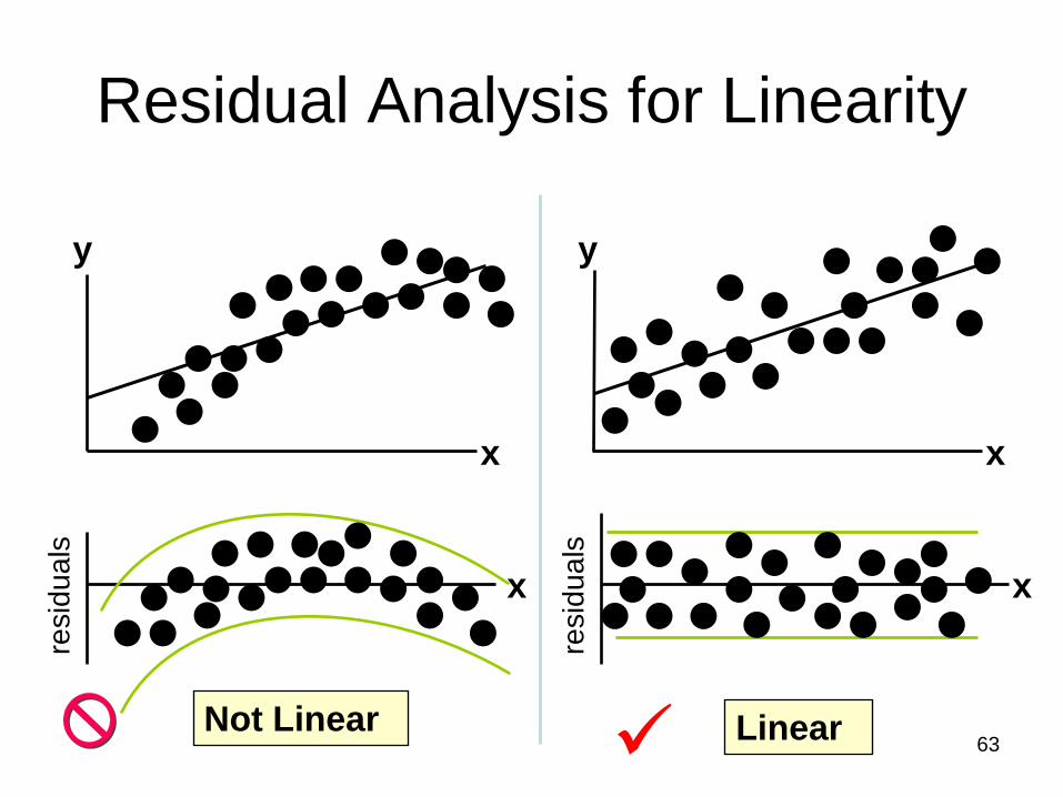
Residual Analysis for Linearity
Not Linear Linear
x
resid
ua
ls
x
y
x
y
x
resid
ua
ls
63

Residual Analysis for Constant Variance
Non-constant variance Constant variance
x x
y
x x
y
resid
ua
ls
resid
ua
ls
64
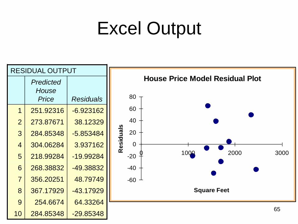
House Price Model Residual Plot
-60
-40
-20
0
20
40
60
80
0 1000 2000 3000
Square Feet
Re
sid
ua
ls
Excel Output
RESIDUAL OUTPUT
Predicted
House
Price Residuals
1 251.92316 -6.923162
2 273.87671 38.12329
3 284.85348 -5.853484
4 304.06284 3.937162
5 218.99284 -19.99284
6 268.38832 -49.38832
7 356.20251 48.79749
8 367.17929 -43.17929
9 254.6674 64.33264
10 284.85348 -29.85348 65

• Thank you.
66