Magnetic Resonance in Medicine 000:000–000 (2011)

Application of the Fractional Fourier Transform to ImageReconstruction in MRI

Vicente Parot,1,2 Carlos Sing-Long,1,2 Carlos Lizama,2,3 Cristian Tejos,1,2 Sergio Uribe,2,4

and Pablo Irarrazaval1,2*

The classic paradigm for MRI requires a homogeneous B0 fieldin combination with linear encoding gradients. Distortions areproduced when the B0 is not homogeneous, and several post-processing techniques have been developed to correct them.Field homogeneity is difficult to achieve, particularly for short-bore magnets and higher B0 fields. Nonlinear magnetic com-ponents can also arise from concomitant fields, particularly inlow-field imaging, or intentionally used for nonlinear encoding.In any of these situations, the second-order component is key,because it constitutes the first step to approximate higher-orderfields. We propose to use the fractional Fourier transform foranalyzing and reconstructing the object’s magnetization underthe presence of quadratic fields. The fractional fourier trans-form provides a precise theoretical framework for this. We showhow it can be used for reconstruction and for gaining a betterunderstanding of the quadratic field-induced distortions, includ-ing examples of reconstruction for simulated and in vivo data.The obtained images have improved quality compared with stan-dard Fourier reconstructions. The fractional fourier transformopens a new paradigm for understanding the MR signal gen-erated by an object under a quadratic main field or nonlinearencoding. Magn Reson Med 000:000–000, 2011. © 2011 WileyPeriodicals, Inc.

Key words: fractional fourier transform; magnetic resonanceimaging; image reconstruction; field inhomogeneities; off-resonance correction; nonlinear encoding

The standard paradigm for MRI requires a strong mag-netic field with uniform intensity and time-varying linearencoding gradients across the entire field of view. How-ever, deviations in the main field are common as uniformfields are physically difficult to achieve and also becauseof off-resonance effects from susceptibility changes. Suchfrequency variations introduce an accumulating phase overtime, which cannot be demodulated easily as it varies spa-tially. This problem is worse for stronger fields and forsequences with long acquisition times. Great efforts are put

1Department of Electrical Engineering, Pontificia Universidad Católica deChile, Santiago, Chile2Department of Electrical Engineering and Department of Radiology, PontificiaUniversidad Catolica de Chile, Santiago, Chile3Department of Mathematics and Computer Science, Universidad de Santiagode Chile, Santiago, Chile4Department of Radiology, Pontificia Universidad Católica de Chile, Santiago,ChileGrant sponsor: CONICYT; Grant number: Fondecyt 1070674 and 1100529,FONDEF D05I10358, and Anillo PBCT-ACT-79*Correspondence to: P. Irarrazaval, Ph.D., Department of Electrical Engineer-ing, Pontificia Universidad Catolica de Chile, Av. Vicuna Mackenna 4860,Macul 7820436, Santiago, Chile. E-mail: pim@ing.puc.clReceived 11 January 2011; revised 21 July 2011; accepted 28 July 2011.DOI 10.1002/mrm.23190Published online in Wiley Online Library (wileyonlinelibrary.com).

in building the system with the highest possible homogene-ity, for example, with passive or active shimming whichpartially correct first- and second-order field variations.

Additionally, there has been an increasing interest inspatial encoding by nonhomogeneous, nonbijective spatialencoding magnetic fields (SEMs; Ref. 1). Starting from ageneral nonlinear field concept, novel techniques includ-ing PatLoc (1), O-Space (2), Null Space (3), and Phase-Scrambled imaging (4–6) have all introduced the use ofsecond-order SEMs as the first and simplest approach insimulations, custom-built hardware and experiments (7–12). One of the challenges of these approaches is to havean appropriate reconstruction technique.

Higher-order fields also appear as a natural componentof linear gradients. These concomitant fields can be wellapproximated by quadratic functions (13,14). In severalapplications, the magnitude of these fields is not negligibleand artifacts appear in image reconstructions (15,16), mostnotably in very low-field or microtesla imaging (17,18).

Several image reconstruction methods have been pro-posed to correct distortions, or to reconstruct an imageproduced by nonhomogeneous fields, being an active fieldof research (19–28). There is a well-known theoretical back-ground for the linear correction approaches, in which anexact analytical solution is provided (19,23). For second-order and arbitrary field maps, there are several correctiontechniques that typically trade-off correction accuracy forcomputational load. Some of them are variations of thebasic conjugate phase (CP) approach (29–31), which willbe relevant to this work.

The fractional Fourier transform (FrFT) is a generaliza-tion of the standard Fourier transform (FT) by means of thecontinuous fractional order a, which covers densely theentire transition between image (or time) domain (a = 0)and the Fourier domain (a = 1; Ref. 32). The FrFT is aspecial case of the linear canonical transform and can bedefined in several different ways leading to different phys-ical interpretations and thus, it has become useful in manyapplications (33–35). It has been shown that the FT prop-erties are special cases of FrFT properties (32), and furtherresearch has been done in discretization (36,37), fast com-putation (38), and other aspects of the FrFT related to signalprocessing (39–42).

It is of general knowledge that the magnetization of anobject under a linear magnetic field can be related to the FTof the MR signal due to the mathematical equivalence of thesignal with the FT kernel. Similarly, the magnetization ofan object under a quadratic field can be related to its FrFT.The kernel of the integral definition of the FrFT presentsa resemblance with the MR signal. This fact, along with

© 2011 Wiley Periodicals, Inc. 1

2 Parot et al.

the techniques involving second-order SEMs or concomi-tant fields, places the FrFT as a potentially useful tool dueto its inherent connection with the second-order modula-tion of the MR signal. The Fresnel transform, also a specialcase of the linear canonical transform, has found a partic-ular use in phase-scrambled imaging. The FrFT provides awider description of the problem and a stronger formula-tion through its physical relation to the FT. For the purposesof this work, let a quadratic MR system be one which hasa second-order magnetic field as a function of space, withtime-varying global amplitude. Thus, systems that have aquadratic main field and/or quadratic SEMs fit into thisdescription.

In this article we present a theoretical description of therelationship between the FrFT and the MR signal in thepresence of quadratic fields. This relation provides a the-oretical framework to analyze the distortions produced byquadratic fields and allows to define a reconstruction tech-nique. We show how the FrFT corrects substantial phaseerrors for constant gradient trajectories (two-dimensionaldiscrete Fourier transform (2DFT), for example) and cor-rects geometric distortions for variable gradients trajec-tories, such as echo planar imaging (EPI). Furthermore,we also introduce a variable order FrFT, which turns outto be similar to CP with an added weighting function,although its interest is more theoretical than practical as theimprovements are minor, and CP is more general, becauseit is also applicable to arbitrary field deviations.

THEORY

This section explains the connection between the FrFT andquadratic MR systems. This framework allows to analyzethe acquired data in a fractional order polar space, fromwhere a visual insight can be extracted.

FrFT

The a-th order FrFT fa(ρ) = Fa{f }(ρ) of the signal f (u) for0 < |a| < 2 can be expressed as an integral transform as(taken from Ref. 32 with a slight change of notation)

fa(ρ) = Cα(ρ)∫

f (u)exp(iπ[u2 cot α − 2ρu csc α]) du, [1]

Cα(ρ) ≡ exp(iπρ2 cot α)√

1 − i cot α, α ≡ aπ/2, [2]

where cot is the cotangent, and csc is the cosecant of theargument.

Note that the most notable difference between this equa-tion and the FT is an extra quadratic phase in the kernel.

Throughout this section, u and ρ denote dimension-less variables to maintain formal consistency between theMRI and FrFT contexts. The independent variable ρ is thepseudofrequency in any fractional domain, and u is the par-ticular case of ρ for the 0-th order (the object domain). Therelation between the dimensionless u and its dimensionalcounterpart x will be addressed in the “ρ–α space” section.

MRI Signal Under a Quadratic Main Field

We will consider the one-dimensional case where the mainfield is a quadratic function of space and linear encoding

gradients are used. The extension to general quadratic MRsystems will be discussed later on. Let f (u) be the mag-netization of the object of interest. The MR signal, in aperfect uniform B0 field, ignoring intrareadout T1 and T2

relaxations and after demodulation at the Larmor frequencyω0 is

s(t) =∫

f (u)exp(−i2πk(t)u) du, [3]

where, as customarily defined, k(t) = γ/2π∫ t

0 G(τ)dτ is thek-space trajectory.

Whenever there is an inhomogeneous field B(u) = B0 +p(u) as a function of space, the magnetization is modulatedby a time-dependent phase. For a quadratic field, p(u) =p2u2 + p1u + p0. In this case the signal equation becomes

s(t) = exp(−i2πp0t)

×∫

f (u)exp(iπ[−2p2tu2 − 2(k(t) + p1t)u]) du [4]

There is a remarkable similarity between this expressionand the FrFT defined in Eq. 1. Consequently, it is natural tothink that the FrFT can be used to reconstruct these data.

Link Between the MR Signal and the FrFT

To represent Eq. 4 in the form of Eq. 1, define

α(t) = cot−1(−2p2t) and

ρ(t) = k(t) + p1tcsc α(t)

= k(t) + p1t√1 + 4p2

2t2

[5]

In this definition, both α and ρ are functions of time, but itwill be omitted for the sake of notation simplicity. Considerα ∈ (0, π), which ensures csc α > 0, and cot−1 invertible,so it can be written −2p2t = cot α and −2(k(t) + p1t) =−2ρ csc α. With these variables the signal in Eq. 4 becomes

s(t) = exp(−i2πp0t)∫

f (u)exp(iπ[u2 cot α − 2ρu csc α]) du

Using Eq. 1, the signal equation becomes a time-varyingorder FrFT of the object

s(t) = exp(−i2πp0t)Cα(ρ)−1fa(ρ)

fa(ρ) = exp(i2πp0t)Cα(ρ)s(t).[6]

Note that if α were constant and equal to π/2 (or a = 1),the signal equation is recovered in terms of the standardFT. The advantage of this relation is that it provides a well-known framework for working with quadratic terms in themagnetic field.

The two-dimensional (2D) extension is straightforwardand is shown in the Appendix.

In a quadratic MR system, both the main field and SEMscan be modeled as quadratic functions of space. In this case,it is clear that the signal of Eq. 3 becomes:

s(t) = exp(−i2πp0t)∫

f (u)exp(iπ[h(t)u2 + g(t)u]) du [7]

Application of the FrFT to Image Reconstruction 3

FIG. 1. Examples of typical trajectories over a quadratic field in the polar representation of ρ–α space. a: A constant gradient can berepresented as a circular path. b: A 2DFT bipolar gradient describes two circular arcs. c: The polar graph shows the ρ–α space in the readoutdirection for seven readout echoes of an EPI trajectory. [Color figure can be viewed in the online issue, which is available at wileyonlinelibrary.com.]

for some suitable functions h and g. The change of variablesdefined in Eq. 5 can be used to deduce α and ρ as functionsof t. Therefore, the analysis done for a quadratic main fieldcan be extended to quadratic MR systems with time-varyingquadratic fields. However, what follows focuses on the caseof a quadratic main field and linear gradients. This allows toperform experiments in a standard MR system, as describedin “Materials and Methods” section.

The ρ–α Space

The terms α and ρ in Eq. 5 define a parametric trajectory(ρ(t), α(t)) in what we call the ρ–α space. As α is an angle,this space is conveniently represented in polar coordinates.The trajectory in ρ–α space starts immediately after theexcitation (t = 0) in the frequency or Fourier direction(α = π/2), and as time passes, it curves toward the objectaxis (α = 0). What follows analyzes some common trajec-tories using this framework. For the sake of simplicity, therestriction on maximum slew rate is neglected.

Constant Gradient

Let us assume that the readout gradient G0 is constant andstarts at t = 0, as would be the case in a projection recon-struction sequence. Assume also that the field is purelyquadratic p(u) = p2u2. Linear and constant terms can beignored without loss of generality, because the first is equiv-alent to a change in the amplitude of the gradient, and thesecond can be corrected during the signal demodulation.Then k(t) would be

∫ t0 G0dτ = G0t and the trajectory in ρ–α

space would be

α(t) = cot−1(−2p2t)

ρ(t) = k(t) + p1t√1 + 4p2

2t2= G0t√

1 + 4p22t2

which is the parametric form of a circle centered at(G0/4p2, 0). Figure 1a shows this trajectory assumingp2 < 0. The trajectory asymptotically approaches the objectaxis (α = 0), as t increases. As expected, for small valuesof t, the trajectory deviates little from the frequency axis(α = π/2), and therefore distortions due to field variationsare small.

If p2 tends to zero, the quadratic component of thefield vanishes and the center of the circumference locatedat G0/4p2 tends to infinity. Equivalently, the ρ–α spacetrajectory becomes a straight line in the frequency direction

α(t) = cot−1(−2p2t) = π

2

ρ(t) = G0t√1 + 4p2

2t2= G0t.

Standard 2DFT readout

Considering again that the field is p(u) = p2u2, now assumethat the gradient is formed by a negative pulse of duration t0

followed by a positive one, as is standard in 2DFT readouts.In this case,

k(t) =∫ t

0G(τ)dτ =

{−G0t 0 < t < t0

G0(t − 2t0) t0 < t.

Consequently, the trajectory in ρ–α space is given by

α(t) = cot−1(−2p2t)

ρ(t) = 1√1 + 4p2

2t2×

{−G0t 0 < t < t0

G0(t − 2t0) t0 < t.

This trajectory is formed by two circular arcs. The tra-jectory describes one arc for the negative gradient centeredat (−G0/4p2, 0) and continues on the other one centered at(G0/4p2, −G0t0), which corresponds to the positive gradi-ent as shown in Fig. 1b.

EPI readout

If the gradient were a train of negative and positive pulsesas is used in EPI

G(t) ={−G0 for 0 < t < t0, 3t0 < t < 5t0, . . .

G0 for t0 < t < 3t0, 5t0 < t < 7t0, . . .

the described ρ–α space trajectory would be composed bya series of circular arcs centered at (±G0/4p2, ∓jG0t0/2),j = 0, 1, 2, . . . as shown in Fig. 1c.

4 Parot et al.

FIG. 2. Example of a one-dimensional 2DFT trajectory in the polar representation of ρ–α space represented by the continuous line and itsreconstruction interpretation represented by the dashed line. a: Standard Fourier interpretation. b: Fractional Fourier interpretation. c: Variableorder fractional Fourier interpretation.

Spectroscopy

If the sequence has no gradients, as in a pure spectroscopicacquisition, the trajectory will only depend on the linearterm of the field p1

α(t) = cot−1(−2p2t)

ρ(t) = k(t) + p1t√1 + 4p2

2t2= p1t√

1 + 4p22t2

and will have the shape shown in Fig. 1a, centered at(p1/4p2, 0). If p1 = 0, the trajectory is a singularity at theorigin of the ρ–α space. In this case, it is more convenient torepresent the space in Cartesian coordinates (ρ, a), and thereadout trajectory ρ = 0 becomes equivalent to acquiringthe continuous component of the FrFT for the orders a.

Reconstruction

In the FrFT framework, the reconstruction problemrequires knowing both the pseudofrequency and the trans-form order where the data was acquired. These can bedetermined using Eq. 5. The object will be the solution tothe inverse of Eq. 6 (ignoring the constant field shift p0)

f (u) = F−a{fa(t)(ρ(t))}(u) = F−a{Cα(t)(ρ(t))s(t)}(u).

This expression explicits the time dependence of α. Thisdependency implies that the fractional order changes withtime and therefore a standard inverse FrFT is not possi-ble. We propose two alternatives for the reconstruction:the inverse FrFT, which assumes an approximation forthe ρ–α space; and the variable order inverse fractionalFourier reconstruction (VO-FrFT). These techniques arecompared with the standard inverse Fourier reconstruc-tion (FT). Figure 2 shows the actual ρ–α space trajectory andthe assumption of the reconstruction scheme for a standard2DFT readout.

Standard Inverse Fourier Reconstruction

This is equivalent to assuming that α ≡ π/2, cot α ≡ 0 andCπ/2(ρ) ≡ 1. The reconstructed object is

f (u) = F−1{s(t)}(u).

The samples are acquired in the curved trajectory but areinterpreted as being in the frequency axis (vertical dashedline of Fig. 2a). The distortions in the image will depend onhow much the trajectory deviates from the vertical line inthe ρ–α space . This reconstruction can be computed usingthe FFT algorithm.

Inverse Fractional Fourier Reconstruction

It assumes that the samples are acquired at a constant order,i.e. on a straight line in ρ–α space during readout, and thatlocations along the fractional domain are uniformly spaced.

The reconstruction and sampling locations are closerthan in the FT reconstruction and the inverse expression isexactly an inverse FrFT

f (u) = F−a{Cα(ρ(t))s(t)}(u),

where a (or α) is the order (or angle for the straight line) atthe origin. This reconstruction is a better approximationand improves the accuracy of the reconstructed object’sphase over the standard Fourier reconstruction. Using thedefinitions in Eqs. 1 and 2, it can be seen that

f (u) = exp(−iπu2 cot α)| csc α|∫

s(t)exp(i2πuρ csc α) dρ.

[8]

In the case of a sequence with multiple echoes duringone readout, this approximation may not be useful as thetrajectory differs from a single constant line and the originis sampled with multiple different angles. In the case of anEPI readout (Fig. 1c), the trajectory can be approximatedwith a constant angle for each echo, which approximatesbetter the angle of each sample. Reconstruction using theinverse FrFT can be implemented using any of the discretealgorithms available in the literature (32), with computa-tion complexity O(N log N ) and additional overhead timeswhen compared with FFT.

Variable Order Inverse Fractional Fourier Reconstruction

This approach uses the actual locations where the datawere acquired. To solve the variable order inverse prob-lem we propose a discrete approach, which fits well withthe discrete samples and can also provide a continuous

Application of the FrFT to Image Reconstruction 5

reconstruction. Each sample in ρ–α space (ρn, αn) acquiredat t = tn corresponds to one coefficient of the FrFT of orderan = 2αn/π. Each of these coefficients is the projection ofthe object into the kernel function of the correspondingfractional order and position. These kernels are commonlyknown as “chirp” functions and are given by the inverseFrFT of order an of a delta function located at ρ = ρn (32):

∆−an (u) = F−an {δ(ρ − ρn)}(u)

= C*αn

(ρn) exp(−iπ[u2 cot αn − 2uρn csc αn]),

where * denotes complex conjugate. From the set of allpossible chirp functions, the object is projected to the sub-set of (ρn, αn) pairs corresponding to the sampling locationstraversed by the trajectory during readout. Reconstructionfrom these coefficients is feasible as long as the trajec-tory is well conditioned. In a discrete sense, this meansthat the trajectory and sampling locations must define anapproximately orthogonal square encoding matrix. Fromthis general idea, whenever a well-conditioned trajectoryand uniform sampling density is used, a simple sum of thecontributions of each projection can give a good estima-tion of the generating object. Recalling that the samples aredefined by

fan (ρn) = Cαn (ρn)s(tn),

this yields an estimation of the object as the weighted sumof all contributions, one for each of N samples,

f (u) =N∑

n=1

fan (ρn)∆−an (u)

=N∑

n=1

| csc αn|s(tn)exp(−iπ[u2 cot αn − 2uρn csc αn]).[9]

If the uniform sampling density assumption is dropped,it would be necessary to incorporate a factor proportionalto ρ(tn) which arises from the underlying discretization ofthe inverse FrFT integral by Riemann sums. To use thisreconstruction method with 2DFT and EPI trajectories, itis assumed that they are approximately well conditionedwithin a limited quadratic field component, as they areinherently designed for k-space acquisition and not tomatch ρ–α space positions of orthogonal projections.

The nominal computational complexity of this methodis O(N 2), and its implementation cannot be based on theFFT. The 2D extension of this reconstruction method ispresented in the Appendix.

The object f (u) in Eq. 9 can be evaluated for any contin-uous value of u. Note that if αn is substituted by π/2 thisformula becomes the definition of the discrete frequencyFourier transform, or the Discrete Fourier Transform (DFT),if u is also evaluated at discrete values. If αn is substitutedby another fixed angle, other than π/2, the reconstructionis also the discrete frequency fourier transform, but with anextra phase and an additional constant scaling factor. Thisis the discrete version of the inverse FrFT.

It is relevant to note that the CP method reconstructsremoving the phase modulation due to field inhomogeneity

from the signal. In one dimension and with uniform sam-pling density, the CP reconstruction is (29,30)

f (u) =N∑

n=1

s(tn)exp(i2π[knu + tnp(u)]), [10]

where the pair (tn, kn) denotes the sampled trajectory in k-space and p(u) is an arbitrary frequency deviation. Note thatthis method also assumes the trajectory to be well condi-tioned, because the independence of the summed functionsheavily depends on the trajectory and the arbitrary fieldp(u). Considering only the first- and second-order terms ofits Taylor approximation, the inhomogeneity is reduced top(u) = p2u2 + p1u. In this case, the difference between theVO-FrFT and CP can be appreciated in Eq. 9, substitutingthe definitions in Eq. 5, so that VO-FrFT method can bewritten as:

f (u) =N∑

n=1

| csc αn|s(tn)exp(i2π[knu + tnp(u)]).

Notably, the VO-FrFT method and a second-orderapproximated field CP reconstruction differ in the mod-ulating factor | csc αn|. These weights arise naturally as aconsequence of using the FrFT, assuming uniform k-spacesampling density. Additionally, this relation shows that theimplementation of the VO-FrFT will have a similar compu-tational load as a CP reconstruction method. Consequently,techniques to speed up CP reconstructions can be used forthe same purpose for VO-FrFT reconstructions.

Units

So far, ρ and u have been used as dimensionless variables.To ensure the validity of the former analysis and extend itto practical cases, the normalization u = x/q is used, bywhich

f (u) = f (x/q) = √qf (x) [11]

with f (x) the dimensional object. The scale parameter qhas the same dimension as x. For the purpose of the FrFTimplementation, it can be assumed that the magnetiza-tion is mostly concentrated within the field of view (FOV),whereas its spectrum is mostly concentrated in the sam-pled region of k-space. In the time–frequency plane, thismeans that the energy is mostly concentrated over an ellip-tic region. The suitable parameter for q is the one thattransforms this elliptic region into a circular one. This isachieved by setting q = FOV/

√N (43). This normaliza-

tion is applied independently for each dimension for then-dimensional case.

MATERIALS AND METHODS

The purpose of the experiments is twofold. First, tostudy numerically the problem of recovering an imagefrom the MR signal when the main field is quadraticand the gradients are linear. Second, to prove that ourreconstruction is useful as a field inhomogeneity correc-tion algorithm for images acquired in traditional systemsand when the inhomogeneity has an important quadraticcomponent. All MRI images in this work were acquired

6 Parot et al.

with a Philips Intera 1.5T scanner. Linear shimming wasdisabled during all acquisitions and no higher-order activeshimming was used. The images were acquired usingmostly default parameters from preloaded sequences inthe system. Complex-valued image reconstructions wereperformed off-line.

Numerical Phantom

In our first experiment, the MR signal for a 2D, real-valuedanalytical magnetization phantom was simulated by eval-uating Eq. A1 using adaptive quadrature in MATLAB (44),nesting a one-dimensional evaluation for each dimension.The phantom was designed as a simplified version of areal reference phantom with the same dimensions. Theacquisition time of each sample and k-space locations weredetermined considering 2DFT gradients from a standardacquisition. A cartesian matrix of 256 × 256 samples wassimulated with FOV of 25.6×25.6 cm and echo time (TE) =56 ms. Each complete readout in the sequence takes 28 ms.

Two MR signals were simulated, the first with a uni-form B0 field and the second with a quadratic field withcoefficients p2x = −2.149 Hz/cm2, p2y = −2.3846 Hz/cm2,p1x = 0 Hz/cm, p1y = 0 Hz/cm, and p0 = 0 Hz. Thequadratic deviation was chosen to be approximately doublethe measured quadratic component from a real phantom toenhance the effect (while keeping it within a valid physicalrange). These parameters define the sampling locations ofthe ρ–α space trajectory, of which fractional domain anglesare shown for direction y in Fig. 3 with a solid line. Thereconstructed image with standard FT and uniform B0 wasthe reference image which incorporates all the inherentdistortions of sampling the k-space and the discrete recon-struction. The simulated MR data under a quadratic fieldwas reconstructed with the standard inverse FT, the inverseFrFT, the inverse VO-FrFT, and CP.

To study the performance of these methods when thereis error in the estimation of the quadratic component,the reconstruction was repeated using different values ofp2x and p2y (from 0× to 2× in steps of 0.125×). See theAppendix for a theoretical estimation of uncertainties.

MRI Phantom

In a second experiment, a phantom was scanned with afast field echo (FFE) EPI sequence, with a scan matrix of128×128 samples, FOV of 24×24 cm, slice thickness 5 mm,flip angle 23◦, and Pulse repetition time/TE = 650/41 ms.These data were acquired with a number of sample averagesof 16 using a Q-body coil. The EPI factor in this sequencewas 63. Each complete readout in this sequence took 76 ms.These parameters produce a long readout sequence inwhich there is a noticeable effect of the field inhomo-geneities that are inherent to the MR system and object.For the FrFT a constant angle per echo was used. The FrFTapproach and the VO-FrFT used a quadratic fit for the mea-sured field map, whereas the CP reconstruction used themeasured field map.

In vivo Study

An in vivo study was done scanning the brain of a volun-teer, the images were acquired using the same sequence,

FIG. 3. Fractional angle α(t) throughout the readout of experimentaltrajectories. The horizontal axis shows time in ms, with echo time inthe origin. The solid, dashed, and dotted lines represent the numer-ical phantom, MRI phantom, and in vivo experiments, respectively.[Color figure can be viewed in the online issue, which is available atwileyonlinelibrary.com.]

except for number of sample average which was now 8 andfrom the receiving coil which was now a standard quadra-ture head coil. A slightly angled transversal slice of thebrain was selected where the field showed an importantquadratic component.

Field Maps

In each experiment, structural images were acquired withshort readout time sequences to minimize the effect of fieldinhomogeneity. The magnetic field was measured fromthese images with different TE (45).

To fit quadratic functions to the field maps, a maximumlikelihood method was used that minimizes the weightedsquared error between the measured field map and a para-metric separable second-order polynomial. The weightswere the mean magnitude of the corresponding pixels. Thisensures that the field map information was incorporatedcorrectly depending on the local intensity of the signal andits signal to noise ratio.

In the phantom study, the field map was determinedalong a structural reference image using ∆TE = 3 ms andpulse repetition time and TE equal to 14 and 6.1 ms, respec-tively. A transversal slice of the physical phantom wasselected for this study.

For the in vivo study, the anatomy causes further fielddeviations which cannot be approximated by the fittedfunction for the entire FOV. An elliptical region of interestwas selected.

Image Reconstruction

FT computations were done using FFT and took less than1 s in all cases. FrFT and VO-FrFT reconstructions weredone by computing Eq. A2, which took 10 min for a 256 ×256 matrix and 1.5 min for a 128×128 matrix, with a Quad-Core 2.4 GHz CPU. The FrFT reconstruction used a constantangle value for each echo, using the value of the anglewhen ρu = 0. This is equivalent to compute the 1D inverseFrFT in the readout direction, along which the angles are

Application of the FrFT to Image Reconstruction 7

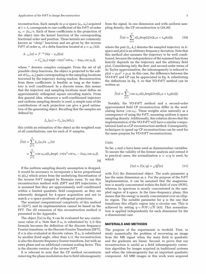
FIG. 4. Reference image for numerical study. This is an inverseFourier reconstruction of an undistorted simulated signal.

assumed to be constant but not in the phase direction,where the angle is different for each sample. For simplicityof implementation, in this work, we did not take advan-tage of the fast implementation of the FrFT which wouldspeed it up considerably. The VO-FrFT reconstruction tookinto account the exact position in ρ–α space of each sam-ple. Distance units of the results were scaled using Eq. 11 tomap the estimated object into the dimensional coordinates.CP reconstructions were computed using the 2D extensionof Eq. 10, with p(u) the exact measured or simulated fre-quency deviation and were found to require essentially thesame computing time as VO-FrFT reconstructions.

RESULTS

To compare the performance of the reconstruction meth-ods, absolute value images were compared using the rootmean squared error (RMSE) and the mean absolute error(MAE). These two metrics heavily penalize images thathave only contrast differences, such as an intensity scaling.

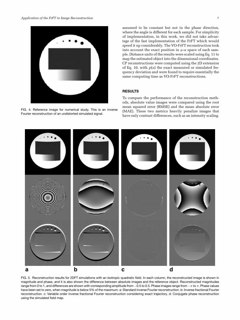
FIG. 5. Reconstruction results for 2DFT simulations with an isotropic quadratic field. In each column, the reconstructed image is shown inmagnitude and phase, and it is also shown the difference between absolute images and the reference object. Reconstructed magnitudesrange from 0 to 1, and differences are shown with corresponding amplitude from −0.5 to 0.5. Phase images range from −π to π. Phase valueshave been set to zero, when magnitude is below 5% of the maximum. a: Standard inverse Fourier reconstruction. b: Inverse fractional Fourierreconstruction. c: Variable order inverse fractional Fourier reconstruction considering exact trajectory. d: Conjugate phase reconstructionusing the simulated field map.

8 Parot et al.

For this reason a third metric was used: mutual informa-tion (46), which is invariant to intensity scaling and isneeded, because in some cases the reference image wasacquired with a different MR contrast than the experimen-tal MR data. Note that, in contrast with the RMSE and theMAE, higher values of mutual information imply that thecompared images are closer to each other.

Numerical phantom

The reference image of the numerical phantom can be seenin Fig. 4. The distortions produced by a quadratic fieldwhen using the standard Fourier reconstruction can beseen in Fig. 5a. It shows a geometric distortion, charac-teristic of data acquired under field inhomogeneity, whichis proportional to the local field deviation from the cen-tral frequency. The phase of the reconstructed image hasa complex quadratic modulation, although the analyticalphantom did not have phase. An intensity nonuniformitydistortion is also noted that can be described as a linearincrease of intensity from the lower to the upper region ofthe phantom. The maximum deviations were within 12%of the correct value. This can be seen also in the inten-sity difference image (Fig. 5a). As expected, the MR dataacquired with a quadratic main field cannot be correctlyrecovered by the FT method.

As expected from Eq. 8, the FrFT reconstruction showsidentical magnitude as the FT reconstruction (Fig. 5a) butwith a phase much closer to the actual phase (Fig. 5b).Indeed, the intensity difference image (Fig. 5b) is similar tothe one produced by the FT reconstruction. Additionally,both approaches are unable to recover exactly the imagegeometry. The VO-FrFT reconstruction (Fig. 5c) recoversthe original image, without any of the image distortions inmagnitude or phase introduced by the FT and FrFT recon-structions. Finally, the CP reconstruction (Fig. 5d) recoversthe geometry of the phantom, but it adds a phase thatdoes not belong to the reference image. The intensity ofthe reconstructed image also shows differences with thereference image, as evidenced by the intensity differenceimage (Fig. 5d). The visual results are supported by the

Table 1Comparison of the Reconstruction Error for the Numerical PhantomStudy.

Method RMSE Mutual information MAE

FT 20.41 1.33 × 105 7.16FrFT 20.41 1.33 × 105 7.16VO-FrFT 1.68 1.58 × 105 0.86CP 5.35 1.48 × 105 2.82

values for the comparison metrics in Table 1. Only theVO-FrFT reconstructs the exact image, outperforming theCP method. Note that this numerical experiment has beendesigned as an ideal case to test the reconstruction of thesimulated MR signal from a quadratic field and does notnecessarily reflect a real setting, where pure quadratic fieldsare not practically ocurring. In many situations, it can alsobe that the phase is discarded, because only the magnitudeimage is of interest. Note also that differences in resultsbetween the VO-FrFT and CP methods arise in this casesolely from the | csc αn| weights present in the VO-FrFTcomputation.

The sensitivity analysis in Fig. 6 shows how the VO-FrFT has the best indexes for all metrics and how thesemetrics deteriorate as the field used for the reconstructiondeviates from the actual field. Note that different metricsdiscriminate differently both methods. The RMSE showsa very close performance of the VO-FrFT and CP methods(Fig. 6a), being both better than FT and FrFT methods upto a scaling factor of 1.85. Considering mutual information,the VO-FrFT outperforms the other three methods for scalefactors as high as 1.9 (Fig. 6b). Considering MAE, the VO-FrFT outperforms all methods for the whole scaling factorrange used.

MRI Phantom

The phantom is shown in Fig. 7 (without distortions). Theparticular combination of our MR system with its intrinsicinhomogeneity and the scanned phantom produced a field

FIG. 6. Measurement of the distortion in absolute reconstructions produced by scaling the quadratic component of the field as an input tothe reconstruction method. a: Root mean squared error. b: Mutual information. c: Mean absolute error. [Color figure can be viewed in theonline issue, which is available at wileyonlinelibrary.com.]

Application of the FrFT to Image Reconstruction 9

FIG. 7. Low-distortion image used as the reference image for thephantom study.

map that resembles an isotropic quadratic function with itshighest intensity in the center of the magnet as shown inFig. 8. The coefficients of the quadratic function were p2x =−1.24 Hz/cm2, p2y = −1.32 Hz/cm2, p1x = −1.81 Hz/cm,p1y = −1.92 Hz/cm, and p0 = 26.29 Hz, and the maximumlikelihood fitting error was 2.11 Hz. A profile of the mea-sured field and its fitted function can be seen in Fig. 8c. The

FIG. 8. Field map fit for the MRI phantom study. a: Measured fieldmap. b: Fitted field map. c: Along the marked column, the measuredmagnetic field (solid line) can be well approximated by a quadraticfunction (dashed line). Field images range from −140 Hz to 40 Hz.[Color figure can be viewed in the online issue, which is available atwileyonlinelibrary.com.]

FIG. 9. Reconstruction results for the MRI phantom study. a: Stan-dard Fourier reconstruction. b: Fractional Fourier reconstructionusing the fitted quadratic field map and constant angle approx-imation in each echo. c: Variable order fractional Fourier recon-struction using the fitted quadratic field map. d: Conjugate phasereconstruction using the measured field map.

trajectory angles determined by the y -direction coefficientsare shown in Fig. 3 with a dashed line.

In this study, the phase information of the object isunknown, because it cannot be acquired with the samecontrast as the distorted object without the effect of thequadratic field map. For this reason, only the magnitude ofthe reconstructions was compared against the magnitudeof the low-distortion image.

The FT reconstruction shown in Fig. 9a produces geo-metric and intensity distortions similar to those observedin the simulation study. The FrFT using constant angleper echoes (Fig. 9b) recovers a better geometry of the sam-ple, albeit with significant Gibbs and ghosting artifacts.Figure 9c shows that the VO-FrFT partially eliminates theseartifacts, correctly reconstructing the geometry and inten-sity of the reference image. We believe that the ghosting arti-facts persist, because the field map is not exactly a quadraticfunction of space. Additionally, some of the artifacts maybe related to an incomplete EPI ghosting correction whichis present in all reconstructions. Finally, the CP reconstruc-tion (Fig. 9d) also recovers the geometry and corrects theghosting artifacts but is unable to correct the Gibbs ringingartifacts. The CP reconstruction additionally shows distor-tions related to noise that are present only in this approach.After CP, the VO-FrFT method has the best reconstruction,as can be seen in Table 2. The difference between VO-FrFTand CP can be explained by a trade-off between the ghost-ing artifacts in the VO-FrFT reconstruction versus the noisepresent in the CP reconstruction.

10 Parot et al.

Table 2Comparison of the Reconstruction Error for the MRI Phantom Study

Method RMSE Mutual information MAE

FT 60.64 1.42 × 105 31.07FrFT 99.89 1.19 × 105 65.31FrFT (c.p.e) 35.08 1.51 × 105 21.28VO-FrFT 33.63 1.51 × 105 19.61CP 28.03 1.59 × 105 15.73

In vivo Study

Figure 10 shows the low-distortion image for the volunteerexperiment. The field can be approximated by a quadraticfunction within an elliptical region of interest as shownin Fig. 11. The coefficients for the fitted quadratic func-tion were p2x = −0.23 Hz/cm2, p2y = −0.78 Hz/cm2,p1x = 0.11 Hz/cm, p1y = 5.28 Hz/cm and p0 = 62.08 Hz,and the maximum likelihood fitting error was 0.09 Hz.The trajectory angles determined by the y -direction coeffi-cients are plotted in Fig. 3 with a dotted line. Figure 10also shows a superimposed contour showing some keygeometric features of the sample, as a visual aid for com-paring the geometric distortions in the reconstructions. TheFT reconstruction (Fig. 12a) presents geometric distortionsin agreement with the artifacts observed in the numericaland phantom experiments. The FrFT reconstruction with

FIG. 10. Low-distortion image used as the reference image for thein vivo study. The superimposed contours show the location of somekey features in the image.

constant angle in each echo (Fig. 12b) corrects most ofthe geometric distortions present in the FT reconstruction(Fig. 12c), especially in the region of interest, where the fit-ted quadratic function is a close approximation of the field

FIG. 11. Field map for the in vivo study. b: Measured field map. c: Fitted field map. Within the elliptical region of interest in (a), the measuredmagnetic field can be approximated by a quadratic function as shown in (d) with solid and dashed lines, respectively, for the marked column.Field images range from −140 Hz to 40 Hz. [Color figure can be viewed in the online issue, which is available at wileyonlinelibrary.com.]

Application of the FrFT to Image Reconstruction 11

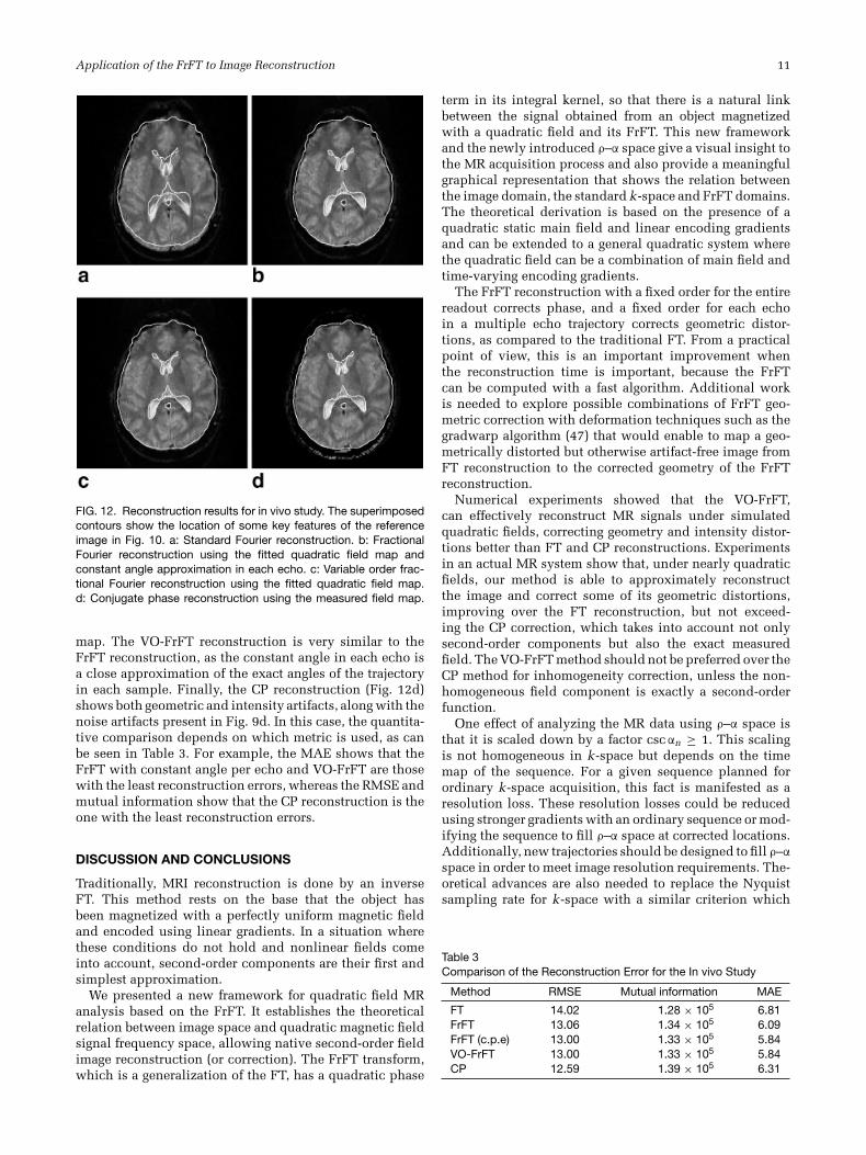
FIG. 12. Reconstruction results for in vivo study. The superimposedcontours show the location of some key features of the referenceimage in Fig. 10. a: Standard Fourier reconstruction. b: FractionalFourier reconstruction using the fitted quadratic field map andconstant angle approximation in each echo. c: Variable order frac-tional Fourier reconstruction using the fitted quadratic field map.d: Conjugate phase reconstruction using the measured field map.

map. The VO-FrFT reconstruction is very similar to theFrFT reconstruction, as the constant angle in each echo isa close approximation of the exact angles of the trajectoryin each sample. Finally, the CP reconstruction (Fig. 12d)shows both geometric and intensity artifacts, along with thenoise artifacts present in Fig. 9d. In this case, the quantita-tive comparison depends on which metric is used, as canbe seen in Table 3. For example, the MAE shows that theFrFT with constant angle per echo and VO-FrFT are thosewith the least reconstruction errors, whereas the RMSE andmutual information show that the CP reconstruction is theone with the least reconstruction errors.

DISCUSSION AND CONCLUSIONS

Traditionally, MRI reconstruction is done by an inverseFT. This method rests on the base that the object hasbeen magnetized with a perfectly uniform magnetic fieldand encoded using linear gradients. In a situation wherethese conditions do not hold and nonlinear fields comeinto account, second-order components are their first andsimplest approximation.

We presented a new framework for quadratic field MRanalysis based on the FrFT. It establishes the theoreticalrelation between image space and quadratic magnetic fieldsignal frequency space, allowing native second-order fieldimage reconstruction (or correction). The FrFT transform,which is a generalization of the FT, has a quadratic phase

term in its integral kernel, so that there is a natural linkbetween the signal obtained from an object magnetizedwith a quadratic field and its FrFT. This new frameworkand the newly introduced ρ–α space give a visual insight tothe MR acquisition process and also provide a meaningfulgraphical representation that shows the relation betweenthe image domain, the standard k-space and FrFT domains.The theoretical derivation is based on the presence of aquadratic static main field and linear encoding gradientsand can be extended to a general quadratic system wherethe quadratic field can be a combination of main field andtime-varying encoding gradients.

The FrFT reconstruction with a fixed order for the entirereadout corrects phase, and a fixed order for each echoin a multiple echo trajectory corrects geometric distor-tions, as compared to the traditional FT. From a practicalpoint of view, this is an important improvement whenthe reconstruction time is important, because the FrFTcan be computed with a fast algorithm. Additional workis needed to explore possible combinations of FrFT geo-metric correction with deformation techniques such as thegradwarp algorithm (47) that would enable to map a geo-metrically distorted but otherwise artifact-free image fromFT reconstruction to the corrected geometry of the FrFTreconstruction.

Numerical experiments showed that the VO-FrFT,can effectively reconstruct MR signals under simulatedquadratic fields, correcting geometry and intensity distor-tions better than FT and CP reconstructions. Experimentsin an actual MR system show that, under nearly quadraticfields, our method is able to approximately reconstructthe image and correct some of its geometric distortions,improving over the FT reconstruction, but not exceed-ing the CP correction, which takes into account not onlysecond-order components but also the exact measuredfield. The VO-FrFT method should not be preferred over theCP method for inhomogeneity correction, unless the non-homogeneous field component is exactly a second-orderfunction.

One effect of analyzing the MR data using ρ–α space isthat it is scaled down by a factor csc αn ≥ 1. This scalingis not homogeneous in k-space but depends on the timemap of the sequence. For a given sequence planned forordinary k-space acquisition, this fact is manifested as aresolution loss. These resolution losses could be reducedusing stronger gradients with an ordinary sequence or mod-ifying the sequence to fill ρ–α space at corrected locations.Additionally, new trajectories should be designed to fill ρ–α

space in order to meet image resolution requirements. The-oretical advances are also needed to replace the Nyquistsampling rate for k-space with a similar criterion which

Table 3Comparison of the Reconstruction Error for the In vivo Study

Method RMSE Mutual information MAE

FT 14.02 1.28 × 105 6.81FrFT 13.06 1.34 × 105 6.09FrFT (c.p.e) 13.00 1.33 × 105 5.84VO-FrFT 13.00 1.33 × 105 5.84CP 12.59 1.39 × 105 6.31

12 Parot et al.

would indicate how information density is distributedalong ρ–α space.

Our approach based on the FrFT gives a new theoreti-cal MR framework between image space and signal spacefor quadratic field MR systems, allowing native imagereconstruction for second-order main fields.

APPENDIX A: EXTENSION TO TWO DIMENSIONS

To extend the correspondence between the signal equa-tion and the FrFT definition derived in “Link Betweenthe MR signal and the FrFT” section, it can be writtenin vector form using the separable FrFT definition. In twodimensions, the FrFT is (32)

fa(ρ) = Cα(ρ)∫

f (u)exp(iπ(uTAu − 2uTBρ))du

with

u =[uv

], ρ =

[ρu

ρv

], a =

[au

av

], α = a

π

2=

[αu

αv

]

A =[cot αu 0

0 cot αv

], B =

[csc αu 0

0 csc αv

]

and Cα(ρ) = √1 − i cot αu

√1 − i cot αv exp(iπρT Aρ).

To write the signal equation in 2D, the field can be writtenas p(u) = uTp2u + uTp1 + p0, with

p1 =[p1u

p1v

]and p2 =

[p2u 00 p2v

],

so that it becomes

s(t) = exp(−i2πp0t)

×∫

f (u)exp(iπ(−2uTp2ut − 2uT(k(t) + p1t)))du [A1]

with k(t) = [ku(t) kv (t)]T, expanded as

s(t) = exp(−i2πp0t)∫∫

f (u, v )exp (−i2π((p2uu2 + p2v v2)t

+ (ku(t) + p1ut)u + (kv (t) + p1v t)v ))dudv .

Note that it is also assumed that the second-order term ofthe field is diagonal in the coordinate axis, i.e. the termsoutside the diagonal of p2 are zero to match the separableform of the FrFT. If this is not the case, a change of variablescan be performed on x, y , and u, v to diagonalize this term.Note that both A and B are diagonal matrices that dependon α. A four-dimensional ρ–α space is defined by the changeof variables

cot αu = −2p2ut

cot αv = −2p2v t

ρu csc αu = ku(t) + p1ut

ρv csc αv = kv (t) + p1v t

which is equivalent to solve for α and ρ the matrix equa-tions A(α) = −2p2t and B(α)ρ = k(t) + p1t. Finally, the

signal equation is expressed in terms of a 2D varying-orderFrFT as

s(t) = exp(−i2πp0t)Cα(ρ)−1fa(ρ)

Similarly, the 2D extension of the reconstruction methodpresented in Eq. 9 is

f (u) =N∑

n=1

| det(Bn)|s(tn)exp(−iπ[uTAnu − 2uTBnρn])[A2]

or, expanding the matrix terms,

f (u, v ) =N∑

n=1

| csc αun csc αvn|s(tn)exp(−iπ[cot αunu2

+ cot αvnv2 − 2ρun csc αunu − 2ρvn csc αvnv ]).

APPENDIX B: SAMPLING ERRORS

In practice, there is a degree of uncertainty on the estimatedvalues tn and kn for the ρ–α space. In the following analy-sis, differences between the real and estimated values aredenoted as δtn and δkn respectively. Additionally, the esti-mation of the values for p2, p1, and p0 will also introduce adegree of uncertainty. The difference between the real andestimated value is denoted as δp2, δp1, and δp0, respec-tively. To perform an accurate analysis and reconstructionusing the proposed method, it is important to determinethe impact of these uncertainties on the computed valuesρn and αn. From Eq. 5, the uncertainty δαn on αn will be, tofirst order

δαn = 2p2

1 + 4p22t2

nδtn + 2tn

1 + 4p22t2

nδp2

The first term decreases quadratically in time, with val-ues proportional to the errors in measuring tn, whereas thesecond term decreases linearly in time, and achieves a max-imum value δp2/2p2, i.e., one-half of the relative error inmeasuring p2. The uncertainty δρn in measuring ρn will be,to first order

δρn = sin αnδkn + tn sin αnδp1

− 4p2tn(kn + p1tn)(p2δtn + tnδp2)(

1 + 4p22t2

n

)3/2

It is clear that the first term remains bounded and pro-portional to the error in measuring kn. The second termproduces an error that increases in time proportionally tothe uncertainty in measuring p1. Finally, the third termbehaves as O(knt−2

n ) with respect to δtn, O(t−1n ) with respect

to δtn and O(1) with respect to δp2.

REFERENCES

1. Hennig J, Welz A, Schultz G, Korvink J, Liu Z, Speck O, Zaitsev M.Parallel imaging in non-bijective, curvilinear magnetic field gradients:a concept study. Magn Reson Mater Phys, Biol Med 2008;21:5–14.

2. Stockmann J, Ciris P, Galiana G, Tam L, Constable R. O-space imag-ing: highly efficient parallel imaging using second-order nonlinearfields as encoding gradients with no phase encoding. Magn Reson Med2010;64:447–456.

Application of the FrFT to Image Reconstruction 13

3. Tam L, Stockmann JP, Constable RT. Null Space Imaging: a Novel Gra-dient Encoding Strategy for Highly Efficient Parallel Imaging. In: Proc.Joint Annual Meeting ISMRM-ESMRMB, 2010; p. 2868.

4. Wedeen V, Chao Y, Ackerman J. Dynamic range compression in MRIby means of a nonlinear gradient pulse. Magn Reson Med 1988;6:287–295.

5. Ito S, Yamada Y. Alias-free image reconstruction using Fresnel transformin the phase-scrambling Fourier imaging technique. Magn Reson Med2008;60:422–430.

6. Zaitsev M, Schultz G, Hennig J. Extended Anti-Aliasing Reconstructionfor Phase-Scrambled MRI with Quadratic Phase Modulation. In: Proc.ISMRM, 2009; p. 2859.

7. Schultz G, Weber H, Gallichan D, Hennig J, Zaitsev M. Image recon-struction from radially acquired data using multipolar encoding fields.In: Proc. Joint Annual Meeting ISMRM-ESMRMB, 2010; p. 82.

8. Haas M, Ullmann P, Schneider JT, Ruhm W, Hennig J, Zaitsev M.Large tip angle parallel excitation using nonlinear non-bijective pat-loc encoding fields. In: Proc. Joint Annual Meeting ISMRM-ESMRMB,2010; p. 4929.

9. Lin FH, Vesanen P, Witzel T, Ilmoniemi R, Hennig J. Parallel ImagingTechnique Using Localized Gradients (Patloc) Reconstruction UsingCompressed Sensing (cs). In: Proc. Joint Annual Meeting ISMRM-ESMRMB, 2010; p. 546.

10. Cocosco1 CA, Dewdney AJ, Dietz P, Semmler M, Welz AM, GallichanD, Weber H, Schultz G, Hennig J, Zaitsev M. Safety Considerations fora Patloc Gradient Insert Coil for Human Head Imaging. In: Proc. JointAnnual Meeting ISMRM-ESMRMB, 2010; p. 3946.

11. Welz AM, Gallichan D, Cocosco C, Kumar R, Jia F, Snyder J, Dewd-ney A, Korvink J, Hennig J, Zaitsev M. Characterisation of a PatlocGradient Coil. In: Proc. Joint Annual Meeting ISMRM-ESMRMB, 2010;p. 1527.

12. Stockmann JP, Constable RT. An assessment of o-space imaging robust-ness to local field inhomogeneities. In: Proc. Joint Annual MeetingISMRM-ESMRMB, 2010; p. 549.

13. Bernstein MA, Zhou XJ, Polzin JA, King KF, Ganin A, Pelc NJ, GloverGH. Concomitant gradient terms in phase contrast MR: analysis andcorrection. Magn Reson Med 1998;39:300–308.

14. King KF, Ganin A, Zhou XJ, Bernstein MA. Concomitant gradient fieldeffects in spiral scans. Magn Reson Med 1999;41:103–112.

15. Sica CT, Meyer CH. Concomitant gradient field effects in balancedsteady-state free precession. Magn Reson Med 2007;57:721–730.

16. Du YP, Zhou XJ, Bernstein MA. Correction of concomitant magneticfield-induced image artifacts in nonaxial echo-planar imaging. MagnReson Med 2002;48:509–515.

17. Yablonskiy DA, Sukstanskii AL, Ackerman JJ. Image artifacts in verylow magnetic field MRI: the role of concomitant gradients. J Magn Reson2005;174:279–286.

18. Myers WR, Mossle M, Clarke J. Correction of concomitant gradient arti-facts in experimental microtesla MRI. J Magn reson 2005;177:274–284.

19. Akel JA, Rosenblitt M, Irarrazaval P. Off-resonance correction using anestimated linear time map. Magnetic Reson Imaging 2002;20:189–198.

20. Chen W, Meyer CH. Semiautomatic off-resonance correction in spiralimaging. Magn Reson Med 2008;59:1212–1219.

21. Chen W, Sica CT, Meyer CH. Fast conjugate phase image reconstructionbased on a chebyshev approximation to correct for b0 field inhomogene-ity and concomitant gradients. Magn Reson Med 2008;60:1104–1111.

22. Fessler JA, Lee S, Olafsson VT, Shi HR, Noll DC. Toeplitz-based iter-ative image reconstruction for mri with correction for magnetic fieldinhomogeneity. IEEE Trans Signal Process 2005;53:3393–3402.

23. Irarrazabal P, Meyer CH, Nishimura DG, Macovski A. Inhomogene-ity correction using an estimated linear field map. Magn Reson Med1996;35:278–282.

24. Manjón JV, Lull JJ, Carbonell-Caballero J, García-Martí G, Martí-BonmatíL, Robles M. A nonparametric MRI inhomogeneity correction method.Med Image Anal 2007;11:336–345.

25. Noll DC, Fessler JA, Sutton BP. Conjugate phase MRI reconstruction withspatially variant sample density correction. IEEE Trans Med Imaging2005; 24:325–336.

26. Sutton BP, Noll DC, Fessler JA. Fast, iterative image reconstruction forMRI in the presence of field inhomogeneities. IEEE Trans Med Imaging2003;22:178–188.

27. Vovk U, Pernus F, Likar B. Mri intensity inhomogeneity correc-tion by combining intensity and spatial information. Phys Med Biol2004;49:4119–4133.

28. Lee JY, Greengard L. The type 3 nonuniform fft and its applications.J Comput Phys 2005;206:1–5.

29. Maeda A, Sano K, Yokoyama T. Reconstruction by weighted corre-lation for MRI with time-varying gradients. IEEE Trans Med Imaging1988;7:26–31.

30. Noll DC, Meyer CH, Pauly JM, Nishimura DG, Macovski A. A homo-geneity correction method for magnetic resonance imaging with time-varying gradients. IEEE Trans Med Imaging 1991;10:629–637.

31. Schomberg H. Off-resonance correction of MR images. IEEE Trans MedImaging 1999;18:481–495.

32. Ozaktas HM, Kutay MA, Zalevsky Z, The fractional Fourier transformwith applications in optics and signal processing. Chichester, NY: Wiley,2001.

33. Ozaktas HM, Mendlovic D. Fourier transforms of fractional order andtheir optical interpretation. Opt Commun 1993;101:163–169.

34. Ozaktas HM, Mendlovic D. Fractional Fourier optics. J Opt Soc Am A1995;12:743–751.

35. Yetik IS. Image representation and compression with the fractionalFourier transform. Opt Commun 2001;197:275–278.

36. Candan C, Kutay MA, Ozaktas HM. The discrete fractional Fouriertransform. IEEE Trans Signal Process 2000;48:1329–1337.

37. Ozaktas HM, Sumbul U. Interpolating between periodicity and discrete-ness through the fractional Fourier transform. IEEE Trans Signal Process2006;54:4233–4243.

38. Bultheel A. Computation of the fractional Fourier transform. ApplComput Harmonic Anal 2004;16:182–202.

39. Guven HE, Ozaktas HM, Cetin AE, Barshan B. Signal recovery frompartial fractional Fourier domain information and its applications. IETSignal Process 2008;2:15–25.

40. Ozaktas HM, Barshan B, Mendlovic D, Onural L. Convolution, filtering,and multiplexing in fractional Fourier domains and their relation tochirp and wavelet transforms. J Opt Soc Am 1994;11:547–559.

41. Ozaktas HM, Arikan O, Kutay MA, Bozdagt G. Digital computation of thefractional Fourier transform. IEEE Trans Signal Process 1996;44:2141–2150.

42. Ozaktas HM, Barshan B, Mendlovic D. Convolution and filtering infractional Fourier domains. Opt Rev 1994;1:15–16.

43. Koc A, Ozaktas HM, Candan C, Kutay MA. Digital computation oflinear canonical transforms. IEEE Trans Signal Process 2008;56:2383–2394.

44. Shampine LF. Vectorized adaptive quadrature in matlab. J Comput ApplMath 2008;211:131–140.

45. Schneider E, Glover G. Rapid in vivo proton shimming. Magn ResonMed 1991;18:335–347.

46. Pluim J, Maintz J, Viergever M. Mutual information based registrationof medical images: a survey. IEEE Trans Med Imaging 2003;22:986–1004.

47. Glover GH, Pelc NJ (inventors). Method for correcting image distortiondue to gradient nonuniformity. US patent 4,591,789. December 23, 1983.Assignee: General Electric Company.