application and prospect of orthogonal on-off keying as an

University of North DakotaUND Scholarly Commons

Theses and Dissertations Theses, Dissertations, and Senior Projects

January 2014

Application And Prospect Of Orthogonal On-OffKeying As An Error Control Coding In LaserCommunicationTasbirun Nahian Upal

Follow this and additional works at: https://commons.und.edu/theses

This Thesis is brought to you for free and open access by the Theses, Dissertations, and Senior Projects at UND Scholarly Commons. It has beenaccepted for inclusion in Theses and Dissertations by an authorized administrator of UND Scholarly Commons. For more information, please [email protected].

Recommended CitationUpal, Tasbirun Nahian, "Application And Prospect Of Orthogonal On-Off Keying As An Error Control Coding In LaserCommunication" (2014). Theses and Dissertations. 1602.https://commons.und.edu/theses/1602

https://commons.und.edu?utm_source=commons.und.edu%2Ftheses%2F1602&utm_medium=PDF&utm_campaign=PDFCoverPages

https://commons.und.edu/theses?utm_source=commons.und.edu%2Ftheses%2F1602&utm_medium=PDF&utm_campaign=PDFCoverPages

https://commons.und.edu/etds?utm_source=commons.und.edu%2Ftheses%2F1602&utm_medium=PDF&utm_campaign=PDFCoverPages

https://commons.und.edu/theses?utm_source=commons.und.edu%2Ftheses%2F1602&utm_medium=PDF&utm_campaign=PDFCoverPages

https://commons.und.edu/theses/1602?utm_source=commons.und.edu%2Ftheses%2F1602&utm_medium=PDF&utm_campaign=PDFCoverPages

mailto:[email protected]

APPLICATION AND PROSPECT OF ORTHOGONAL ON-OFF KEYING AS AN

ERROR CONTROL CODING IN LASER COMMUNICATION

By

Tasbirun Nahian Upal

Bachelor of Science, University of Dhaka 2008

Master of Science, University of Dhaka 2010

A Thesis

Submitted to the Graduate Faculty

of the

University of North Dakota

in partial fulfillment of the requirements

for the degree of

Master of Science

Grand Forks, North Dakota

May

2014

ii

© Copyright 2014 Tasbirun Nahian Upal

And

Dr. Saleh Faruque

iii

This thesis, submitted by Tasbirun Nahian Upal in partial fulfillment of the requirements for

the Degree of Master of Science from the University of North Dakota, has been read by the

Faculty Advisory Committee under whom the work has been done and is hereby approved.

_______________________________________

Dr. Saleh Faruque

_______________________________________

Dr. William Semke

_______________________________________

Dr. Prakash Ranganathan

This thesis is being submitted by the appointed advisory committee as having met all of the

requirements of the School of Graduate Studies at the University of North Dakota and is

hereby approved.

____________________________________

Wayne Swisher

Dean of the School of Graduate Studies

____________________________________

Date

iv

PERMISSION

Title Application and Prospect of Orthogonal On-Off Keying as an Error

Control Coding in Laser Communication

Department Electrical Engineering

Degree Master of Science

In presenting this thesis in partial fulfillment of the requirements for a graduate

degree from the University of North Dakota, I agree that the library of this

University shall make it freely available for inspection. I further agree that

permission for extensive copying for scholarly purposes may be granted by the

professor who supervised my thesis work or, in his absence, by the Chairperson of

the department or the dean of the School of Graduate Studies. It is understood that

any copying or publication or other use of this thesis or part thereof for financial

gain shall not be allowed without my written permission. It is also understood that

due recognition shall be given to me and to the University of North Dakota in any

scholarly use which may be made of any material in my thesis.

Tasbirun Nahian Upal

March 14th

, 2014

v

TABLE OF CONTENTS

LIST OF FIGURES ....................................................................................................... viii

LIST OF TABLES ............................................................................................................ x

ACKNOWLEDGMENTS ............................................................................................... xi

ABSTRACT ..................................................................................................................... xii

CHAPTER

1. COMMUNICATION AND CODING .............................................................. 1

1.1 Introduction .............................................................................................. 1

1.2 Importance of Coding ............................................................................... 1

1.3 Typical coding schemes ........................................................................... 3

1.4 LASER communication over RF ............................................................. 3

1.5 Prospect of O3K in LASER ...................................................................... 5

2. COMMUNICATION USING LASER ............................................................. 7

2.1 Introduction .............................................................................................. 7

2.2 Laser communication ............................................................................... 7

2.3 Transmitter ............................................................................................... 8

2.4 Receiver .................................................................................................... 8

2.5 Intensity Modulation ................................................................................ 9

2.6 Analog Modulation ................................................................................. 10

2.7 Digital Modulation ................................................................................. 10

vi

3. ERROR CORRECTION METHODS AND PROPOSED RESEARCH .... 11

3.1 Introduction ............................................................................................ 11

3.2 Error detection processes ........................................................................ 11

3.3 Error correction processes ...................................................................... 12

3.4 Automatic Repeat Request (ARQ) ......................................................... 13

3.5 Forward Error Correction (FEC) ............................................................ 13

3.6 Conventional Block Coding ................................................................... 13

3.7 Orthogonal codes .................................................................................... 17

3.8 Decoding of Orthogonal Code and Error Correction ............................. 17

4. ERROR CONTROL AND BANDWIDTH OPTIMIZATION USING

ORTHOGONAL CODE ................................................................................. 20

4.1 Introduction ............................................................................................ 20

4.2 Properties of Orthogonal Code ............................................................... 21

4.3 Encoding of the data ............................................................................... 23

4.4 Preparation of test bed ............................................................................ 24

4.5 Bandwidth Optimization ........................................................................ 27

5. EXPERIMETAL RESULT ............................................................................. 31

5.1 Introduction ............................................................................................ 31

5.2 Hardware and Software .......................................................................... 31

5.3 Construction of the Experiment ............................................................. 33

5.3.1 Selection of data file ........................................................................ 33

5.3.2 Mapping of the data ......................................................................... 34

5.3.3 Introduction of errors ....................................................................... 34

vii

5.3.4 Choice of bit rate .............................................................................. 34

5.3.5 Conversion into wave file ................................................................ 34

5.3.6 Sending out the bits .......................................................................... 35

5.3.7 Amplification ................................................................................... 35

5.3.8 Operation of laser ............................................................................. 35

5.3.9 Detection and logging of the signal ................................................. 35

5.3.10 Recording of the data ..................................................................... 36

5.3.11 Data retrieval and error correction ................................................. 36

5.3.12 Visual pattern of the 8 bit mapped transmission and reception ..... 38

5.3.13 Visual pattern of the 16 bit mapped transmission and reception ... 39



5.3.16 Summary of LASER reception results ........................................... 42

5.3.17 Summary of wired reception results .............................................. 44

5.4 Bit Error Rate and performance analysis ................................................ 46

6. FUTURE WORK AND CONCLUSION ........................................................ 55

APPENDICES ................................................................................................................. 58

REFERENCES ................................................................................................................ 80

viii

LIST OF FIGURES

Figure Page

1.1 (a) Block diagram of conventional block coding transmission .................................... 6

1.1 (b) Block diagram of orthogonal coding transmission ................................................. 6

2.1 Block Diagram of experimental setup .......................................................................... 9

3.1. (a) XOR operation...................................................................................................... 14

3.1. (b) (n,k) block code .................................................................................................... 14

3.1. (c) Parity check for encoded block ............................................................................ 14

3.2: (a) Encoded block ...................................................................................................... 15

3.2: (b) Error correction by parity bits .............................................................................. 15

3.3: Decoding process of orthogonal code ........................................................................ 18

4.1. Expansion of Hadamard Matrix ................................................................................. 20

4.2 Transmission end steps in flowchart ........................................................................... 25

4.3 Reception end steps in flowchart ................................................................................ 26

4.4 Bit Splitting, 4-bit input and 16x8 mapping ............................................................... 29

4.5 Bit Splitting, 2*3-bit input and 2*(8x8) mapping ....................................................... 29

4.6 Bit Splitting, 4*2-bit input and 4*(4x8) mapping ....................................................... 30

5.1 (a) LASER for data transmission ................................................................................ 32

5.1 (b) Photo-detector (LASER on) .................................................................................. 32

5.1 (c) Photo-detector (LASER off).................................................................................. 32

5.2 (a) 8 bit mapping, 1 error in every 8 bit, 4 kHz transmission ..................................... 38

ix

5.2 (b) 8 bit mapping, 2 errors in every 8 bit, 4 kHz transmission ................................... 38

5.3 (a) 8 bit mapping, 1 error in every 8 bit, 8 kHz transmission ..................................... 38

5.3 (b) 8 bit mapping, 2 errors in every 8 bit, 8 kHz transmission ................................... 38

5.4 (a) 16 bit mapping, 3 errors in every 16 bit, 4 kHz transmission ............................... 39

5.4 (b) 16 bit mapping, 4 errors in every 16 bit, 4 kHz transmission ............................... 39







5.8 (a) 64 bit mapping, 15 errors in every 64 bit, 4 kHz transmission ............................. 41

5.8 (b) 64 bit mapping, 16 errors in every 64 bit, 4 kHz transmission ............................. 41

5.9 (a) 64 bit mapping, 15 errors in every 64 bit, 8 kHz transmission ............................. 41

5.9 (b) 64 bit mapping, 16 errors in every 64 bit, 8 kHz transmission ............................. 41

5.10 BER performances for 8/16/32/64/128/256/512 bit bi-orthogonal

codes- wide scale view............................................................................................. 48

5.11 BER performances for 8/16/32/64/128/256/512 bit bi-orthogonal

code- zoomed view. ................................................................................................. 48

5.12 BER Performance for regular block Codes.. ............................................................ 49

5.13 Change in code rate for different code lengths of bi-orthogonal mapping ............. 52

5.14 Percentage of error correction with respect to code length ....................................... 53

x

LIST OF TABLES

Table Page

3.1 Parity bits estimation................................................................................................... 16

3.2 Relation between code length and number of corrected errors ................................... 19

4.1 n = 8 bit orthogonal and antipodal codes .................................................................... 21

4.2 Bi orthogonal code set ................................................................................................ 22

4.3 (a) mapping table for n = 2 ......................................................................................... 23

4.3 (b) mapping table for n = 4 ........................................................................................ 23

4.4 Expansion of bi-orthogonal matrix size respect to number of bits ............................. 27

4.5 Bit splitting in orthogonal matrix ................................................................................ 28

5.1 Percentage of error correction and code length .......................................................... 33

5.2 Results of error correction for 8 bit data mapping ...................................................... 42

5.3 Results of error correction for 16 bit data mapping .................................................... 42



5.6 Results of error correction for 8 bit data mapping ...................................................... 44




5.10 Change in code rate calculation ................................................................................ 51

5.11 Percentage of error correction with respect to code length ....................................... 53

xi

ACKNOWLEDGMENTS

First, l I express my gratitude to the Department of Electrical Engineering of University

of North Dakota, for giving me the opportunity to research and pursue a master degree

here. My solemn gratitude to Dr. Saleh Faruque who has been a Friend, Philosopher and

Guide. While being my supervisor in this academic period, he has enriched and trained

me with vast knowledge and competitive skills. No words are enough to show how

indebted I am to him for his guidance and support.

I am very much grateful to my advisory committee members, Dr. William Semke, Dr.

Prakash Ranganathan and Dr. Arthur Miles for their continuous support and advice.

Apart from being great advisors, my sincere Thanks to Dr. Semke for allowing me to

work on the Unmanned Aerial Vehicle project and Dr. Ranganathan for letting me to be

his Teaching Assistant. I could not ask for a better advisory committee and mentors for

my graduate study.

I would also like to Thank my friend Riadh Arefin Shuvo who has helped me a lot in

preparing the program for the experiments in this thesis. Thanks to Mr. David Poppke for

his suggestions and support. Also, I would like to mention my gratitude to University of

Dhaka, Bangladesh and Government of Bangladesh for providing me quality education

that prepared the foundation for my higher study.

To my Mom - my idol of Strength and Courage

To my Dad – my idol of Creativity and Patience

xii

ABSTRACT

In this thesis work, a bandwidth efficient coded modulation technique has been proposed

for LASER based communication. It offers reliable error correction and bandwidth

optimization for free space connectivity. Laser communication has been emerging as a

potential alternative of Radio Frequency (RF) communication for long-haul connectivity.

It provides several advantages over RF systems. Some of specific advantages are its high

speed data transfer, higher bandwidth, robust security, immunity to electromagnetic

interference, lower implementation cost. However, as any other communication system, it

requires an error control system that detects and corrects error in the data transmission.

The proposed technique blends well with the laser communication systems to provide a

very good error correction capability. For a decent code length it can correct around 24

percent of error. The proposed method is named as Orthogonal On-Off Keying of

LASER and uses a Bi-orthogonal matrix to generate the encoded data for laser. While

decoding, it uses the cross correlation between two orthogonal codes to detect and correct

any errors during transmission. Orthogonal codes also known as Walsh codes are used for

error correction in Code Divisional Multiple Access of RF communication. But it has not

been investigated for laser systems. Besides on-off keying this code also has enormous

potential in other modulation techniques as well. Here in this thesis project, the error

control performance has been verified using an experimental setup. Furthermore, a

method for more bandwidth efficient transmission of data using laser have been proposed

and discussed. This method of bit splitting offers bandwidth efficiency of unity code rate.

xiii

Altogether, the proposed technique is a promising solution for error detection and

correction and at the same time a bandwidth efficient system.Another advantage of

orthogonal coding is self-synchronization capability as the modulated signals share

orthogonal space as well. All the codes in orthogonal matrix are unique as per their

properties and can be identified separately. As a result, it does not require any

synchronization bits while transmission. This results in reduction of complexity in

implementation and thus yield savings economically.

Like orthogonal matrix, traditional block coding also uses a block of information bits.

Say, they are segmented into a block of k bits. This block is transformed into a larger

block of n bits by adding horizontal and vertical parity bits. This is denoted as (n,k) block

code. The problem with this type of coding is, the added (n-k) bits carry no information

and only helps in error detection and correction. However this bigger block of data can

detect and correct only one error in the transmission and it fails, if more than one error

occurs.

On the other hand, the data is mapped using an orthogonal table in this type of coding

where codes have unique properties. No redundant bits are required to be added as they

possess parity generation property with themselves. Also, the distance property of

orthogonal codes makes it stronger for error detection. For codes of greater length in size,

such approach is capable to correct more than one error.

The test bed is implemented using a LASER transmitter and hardware interface that

includes a computer to receive the data and transmit. The operations such as data capture,

modulation, coding and injection of error are carried by a software written in

MATLAB®. On the receiver side, a high speed photo-detector is placed with a hardware

xiv

interface with another computer. This one has the other part of the program to receive the

bits and decode to extract the transmitted data. To test the error control capability, errors

are intentionally transmitted by altering number of bits in the modulated signal. Upon

reception, the data is compared with the transmitted bits and evaluated. This test goes

through 8, 16, 32 and 64 bits of orthogonally mapped data, several different speed of

transmission and a range of error percentage. All the results were compared and

investigated for prediction and error tolerance.

1

CHAPTER 1

COMMUNICATION AND CODING

1.1 Introduction

Since the dawn of civilization, the field of communication can be identified as the

strongest means of development. Whether it was oral, written or even in the form of sign

language, the purpose is to convey the message and expression to the other individuals.

Nowadays by the word ‘Communication’ generally we refer to the state of the art

technology and most advanced engineering to carry voice, text, picture or any forms of

data to the desired destination. This advanced technology includes wired and wireless

infrastructure. In the wireless communication system, radio signals, ultrasonic, infrasonic

or optical systems are the typical platforms. Lately the communication using Light

Amplification by Stimulated Emission of Radiation (LASER) in the wireless

advancement has become one of the most promising and reliable tool for long distance

line of sight interface. My thesis topic addresses challenges in LASER communication

technology.

1.2 Importance of Coding

To overcome the primary hurdles of digital communication, coding is the solution for it.

The importance of coding does not only reflect that fact that it makes a reliable data

transfer over the channel, it also plays a significant role for error detection and correction.

2

One of the issues in digital data transfer is the security of the data. Data security and

source validation must be ensured in many of those important communications. For

thatpurpose, encrypted data is used and reliable encryption is confirmed by proper coding

scheme.

Another purpose of coding is data compression. This is to make sure that the channel is

best used for its capacity and helps to send more useful data over a limited bandwidth

channel [1]. At the same time, data integrity and validity must be assured. With proper

coding, the best performance to send high volume of data on any channel can be achieved

while the unity of the data need not be compromised.

For data translation, coding plays an important role. It helps to represent the data in

different forms. The significant role of coding in communication is the role of error

detection and correction. Due to channel attenuation, interference and all other

parameters, there are many interruptions and noise introduced to the data while travelling

along the channel. These issues can result in corrupted data, invalid data, irrecoverable

data, damaged data or no data at all. Consequently this causes slower transmission of

data, more repeat requests, and potentially results in a slower communication system.

Proper coding scheme is badly necessary for all these issues to be dealt with. For

correction, detection of error is the first step. So there are schemes that detect the error

and send a repeat request. Also there are coding schemes that can detect and correct the

error by itself. This saves time, channel bandwidth and makes the communication faster.

This thesis is about a coding scheme that we are thinking to apply on LASER

3

communication system which may show the potential of correcting almost 25% of error

by itself.

1.3 Typical coding schemes

There are many coding schemes currently applied in communication systems. Depending

on the channel, bandwidth, noise level, available data compression option, transmitter,

receiver, medium and/or parameters like these the right coding scheme is chosen for a

certain channel. Typical basic categories are source coding and channel coding [2].

In source coding, the data is translated into a stream of bits. ASCII code can be an

example of that. But as this coding scheme has equal length code for all the characters, it

is not considered as efficient as should be. Because in case of characters that have higher

occurrence rate in the communication will take the same space in channel as the lower

occurring ones. Now, by reducing the code length of higher occurring ones, the

performance can be upgraded. So, variable length coding came out to be a choice.

Huffman coding scheme is an example of that.

1.4 LASER communication over RF

Here in this research exploration, we are looking forward to find a reliable, promising and

better solution over existing RF communication system. Especially when a high volume

of data transfer is the point of interest and the bandwidth requirement is high. Also in a

long distance communication where no physical infrastructure is a feasible solution laser

can come up to play a big role. LASER communication has many advantages over RF

systems to get over these points.

4

In terms of data security, laser offers more protection [3]. As the radio frequency is

radiated mostly Omni directional, it can be detected by any receiver in the range. On the

other hand, laser being highly focused and unidirectional, it can be pointed straight to the

receiver and much less likely to be intercept by any invaders. And even if there is an

interception in the middle, it can be easily detectable at the receiver end.

The other promising property of laser transmission is that it can support very high

frequency data transfer. This can go up to gigabits per second which is much higher

when compared to RF data speed. Commercial product is available to support 10 gigabits

per second data transfer in the range of 8200feet [4]. On the other hand for deep space

communication, Lunar Laser Communication Demonstration (LLCD) of The National

Aeronautics and Space Administration (NASA) has proven a laser data transfer of 622

megabits per second. This communication was established between earth and moon

which was a distance of around 239,000 miles [5]. It shows although the laser can offer

high speed connectivity, very long distance may compromise the speed to some extent. In

the RF world, lately offered 4G wireless data speed mentions 50 to 100 megabits per

second of speed for Long Term Evolution (LTE) technology. But outside the lab it

showed capacity of 5-12 megabits per second data transfer [6] [7]. For a wired interface

in data transfer, a gigabit Ethernet network offers 1000 megabits per second transmission

rate. Also a laser system seems to be more cost effective as it does not require any

hardwired infrastructure. A lot of power in RF communication is dissipated in the

ambient even if there is no receiver, whereas laser takes much less power for point to

point communication.

5

Laser is immune to many typical interferences problems that are common issues for RF

systems. Electric discharge, lightning conditions, electromagnetic waves or issues like

these are not a threat on laser beam transmission.

In long range communication, where sending an RF signal can be a costly, unreliable

mean, a laser can be robust solution for it [8]. For an example, deep space

communications or data transfer between space to earth, space to space or even between

air and ground, laser is a promising one to be considered [9].

1.5 Prospect of O3K in LASER

For the modulation of laser to transmit data, on off keying is the most common technique.

In this thesis I am going to review the prospect of the idea of Orthogonal On-Off Keying

to modulate the laser beam. This is a new coding scheme for data transmission. Because

we are looking for a robust data transfer option through laser that will have less error at

the receiver end; The Orthogonal On-Off Keying also written as O3K here in short is

considered as a promising coding scheme to have the self-error correction capability of

around 25%.

This new coding scheme uses code correlation to match data with a look up table and find

if there is any error introduced during transmission. If the number of errors introduced are

within the threshold limit it can correct itself and do not need the data to be retransmitted.

The tradeoff here is that there will be more bits to transmit over the channel. But when

we have a high bandwidth channel like laser, it is better to have some robust means of

transmission in exchange of a few more bits [10].

6

Another advantage of this coding scheme is it is self-synchronized, and does not require

any parity generator. It reduces the complexity of the implementation and makes it more

cost effective. The following Figure 1.1 (a) and 1.1 (b) shows two block diagrams for

comparison between conventional block coding and bi-orthogonal coding for

transmission.

Figure: 1.1 (a) Block diagram of conventional block coding transmission

Figure: 1.1 (b) Block diagram of orthogonal transmission

Data Orthogonal Modulator

Transmitter

Data Parity Generator

Synchronization bits

Modulator Transmitter

7

CHAPTER 2

COMMUNICATION USING LASER

2.1 Introduction

Since the discovery of Light Amplification by Stimulated Emission of Radiation

(LASER) there have been numerous applications of LASER [11]. This includes the fields

of research, medical science, data storage, industrial application, law enforcement and so

forth [3]. Some application examples are of printing, compact disc players, surgery, range

measurements, visual displays etc. and are not only limited to those. As the development

of laser forwards and the size of the equipment decreases, the more and more applications

were invented. The significant reduction of the cost due to the invention of solid state

laser also fueled to propel the number of applications. Application in the communication

field is one of the most optimistic and promising fields of laser application [12].

2.2 Laser communication

Wireless communication is a very important mean of data transfer in the current world.

For long haul communication, remote operations, and deep space data transfer, radio

frequency (RF) based systems have been used for long time. The field of laser

communication has come out to be a reliable alternative to that as it offers a lot of

advantages over it. It is capable to provide very high transfer rate, better security, easy

implementation and maintenance. It does not require any Federal Communication

8

Commission license or frequency allocation in this regard [3]. As long as there is line of

sight available, the implementation of laser communication is feasible. It can be a Local

Area Network(LAN) of a campus or a city, quick replacement or emergency response, or

even air to air or air to ground communication [3].

2.3 Transmitter

In this experiment, for the transmission an off the shelf laser product have been chosen. It

is a class IIIa laser and has a modulated/variable power drive circuit. This laser can be

operated by varying power or sending a modulating signal to the control terminal. It can

support up to 400 KHz of bandwidth with the beam of a 635nm of wavelength. The input

from the data source is amplified by an amplifier as the level of control signal has to be in

the range of 3.0-3.5 Volts. The amplified signal is used to drive the laser and performs

the On-Off keying of the laser.

2.4 Receiver

For the reception unit, a simple PIN diode is used. The response at terminal when

illuminated with the laser can range up to 400 millivolts. This voltage is recorded at the

time domain as it is the data stream. If necessary the voltage is amplified using software

after acquiring the whole signal and storing into the computer. Detailed process is

explained in the experiment section.

If there is a lot of ambient light and probability of saturating the photodetector is high, the

detector may fail to identify the laser signal. To overcome such incidents, a differential

receiver can be designed for better detection [13]. Although in the lab experiment the

9

ambient light saturation was not a concern, but as a future development of the system it

can be considered.

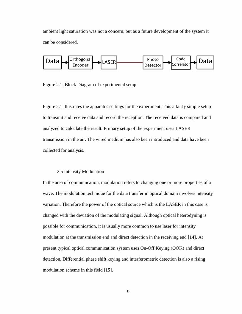
Figure 2.1: Block Diagram of experimental setup

Figure 2.1 illustrates the apparatus settings for the experiment. This a fairly simple setup

to transmit and receive data and record the reception. The received data is compared and

analyzed to calculate the result. Primary setup of the experiment uses LASER

transmission in the air. The wired medium has also been introduced and data have been

collected for analysis.

2.5 Intensity Modulation

In the area of communication, modulation refers to changing one or more properties of a

wave. The modulation technique for the data transfer in optical domain involves intensity

variation. Therefore the power of the optical source which is the LASER in this case is

changed with the deviation of the modulating signal. Although optical heterodyning is

possible for communication, it is usually more common to use laser for intensity

modulation at the transmission end and direct detection in the receiving end [14]. At

present typical optical communication system uses On-Off Keying (OOK) and direct

detection. Differential phase shift keying and interferometric detection is also a rising

modulation scheme in this field [15].

Data Orthogonal

Encoder LASER Photo

Detector

Code Correlator

Data

10

2.6 Analog Modulation

Analog modulation system refers to the continuous modulation of carrier signal with

respect to the information. Some common examples of analog modulations are

Amplitude Modulation (AM), Frequency Modulation (FM), Phase Modulation (PM) etc.

Analog modulation is welcome in short-haul communication and the data can be

retrieved easily. Due to the significant lower cost in implementation and less requirement

for sophisticated equipment, analog modulation is popular in many cases. However in

long distance communication, as there is higher attenuation in the channel it causes more

noise. As such the Signal to Noise Ratio (SNR) for analog modulation becomes less

satisfactory. In those cases digital modulation comes into play [16].

2.7 Digital Modulation

In Digital modulation systems, the carrier signal is modulated using a discrete signal. As

often or most of the time at the user end, the information is an analog distribution, the

system involves analog to digital conversion at the transmission end and digital to analog

conversion at the receiving end. The advantage of digital modulation over the analog one

is discrete change in the states of modulating signal which yields easily detectable binary

states i.e. 0 and 1. Unlike the continuous analog signal, the discrete changes are more

immune to the channel attenuation over the long-haul communication. There are a

number of digital modulation schemes exist. Some examples include but not limited to

Phase Shift Keying (PSK), Frequency Shift Keying (FSK), Amplitude Shift Keying

(ASK), Continuous Phase Modulation (CPM) [16].

11

CHAPTER 3

ERROR CORRECTION METHODS AND PROPOSED RESEARCH

3.1 Introduction

Errors introduced in the channel during the transmission is most obvious and in case of

longhaul communication the error generated is higher due to the attenuation, interference,

impurity, noise and other parameters in the channel. The reliability of data transfer in a

non-ideal channel depends on proper detection and correction of errors. This is also

referred to as the error control technique in the area of communication. Error detection

process identifies the presence of error in the received data and error correction technique

helps to retrieve the original bits and thus confirms the integrity of the received data.

3.2 Error detection processes

Code repetitions: Same set of codes are repeated certain number of time over the channel

and the receiver compares between the repeat blocks. If there is any mismatch found that

blocks are not identical it is certain that errors have been introduced in the channel. This

process is inefficient and if the error occurs in the same manner for all the repeated

blocks, the error is undetectable.

Parity check: In this method a parity bit is added to the block of codes being transmitted.

The count of 1s in the string is predefined as ‘even’ or ‘odd’. Parity bit is attached to

12

maintain the preselected parity check, and at the receiving end the integrity of the data is

checked by verifying the even or odd parity. It is a very simple form of detection and fails

to work if there happens to be even number of errors in the same string which keeps the

parity same.

Checksum: Checksum is computed from the data and can use different algorithms to

generate it. At the receiver the checksum is verified to trace if the data transmitted with it

is error free. Some checksum schemes are parity bits, check digits, and longitudinal

redundancy checks etc. If there is a minor change in the input, a well-built checksum

algorithm should generate significantly different value.

Cyclic redundancy check (CRC): Cyclic redundancy check is not the best to detect

severely generated errors in the channel. It is more likely to be useful in accidental

changes to digital data in computer networks. For detection of burst errors, they work

well. This is hardware friendly in implementation and more common in digital network

and storage media.

3.3 Error correction processes

For error correction it detects and corrects error at the receiver end. Commonly, there are

two methods used in the current communication systems. They are Automatic Repeat

Request (ARQ) and Forward Error Correction (FEC) that approaches use of Error

Correcting Codes (ECC). In case of communications where low latency is not acceptable,

the ARQ is not a feasible option. ARQ requires having a return channel to work so

simplex system is not supported. For a communication like broadcasting or so, ARQ is

less preferred whereas ECC is used.

13

3.4 Automatic Repeat Request (ARQ)

Automatic Repeat Request uses error detection codes along with acknowledgement,

negative acknowledgement and timeout. Upon receiving the data without an error the

receiver sends a positive acknowledgment or otherwise the transmission end gets a

negative response. Negative response triggers to resend the data till it is delivered error

free. Also there is a timeout period if no acknowledgment is received by that time, it is

resent. This type of correction requires duplex communication. And depending on the

channel attenuation and noise the number of repeat request can be fairly high.

3.5 Forward Error Correction (FEC)

In this method upon detection of an error, it is corrected at the receiver end without the

data being resend. Redundant data bits are introduced and attached to the desired data

before transmission. If there is an error introduced in the channel, the receiver can correct

up to certain number of errors (depending on the code) by matching the received bits with

a lookup table. FEC codes can be distinguished in to major categories.

Convolutional code: Data is coded in bit by bit process.

Block code: Data is coded in block by block process.

The experiment here is focused on the Orthogonal coding for error correction which is a

block code for forward error correction.

3.6 Conventional Block Coding

For block coding of the data, the information bits are first segmented into a block of k

bits. Then horizontal and vertical parity bits are generated and a new block is formed.

The number of bits in the new block is n and the segment is called (n,k) block code.

14

Obviously n>k here and a term ‘code rate’ denotes the k/n ratio. Therefore this new

block of codes is transmitted through the channel. Included parity bits (n-k) only

participate to detect and correct errors and do not contain any information [17].

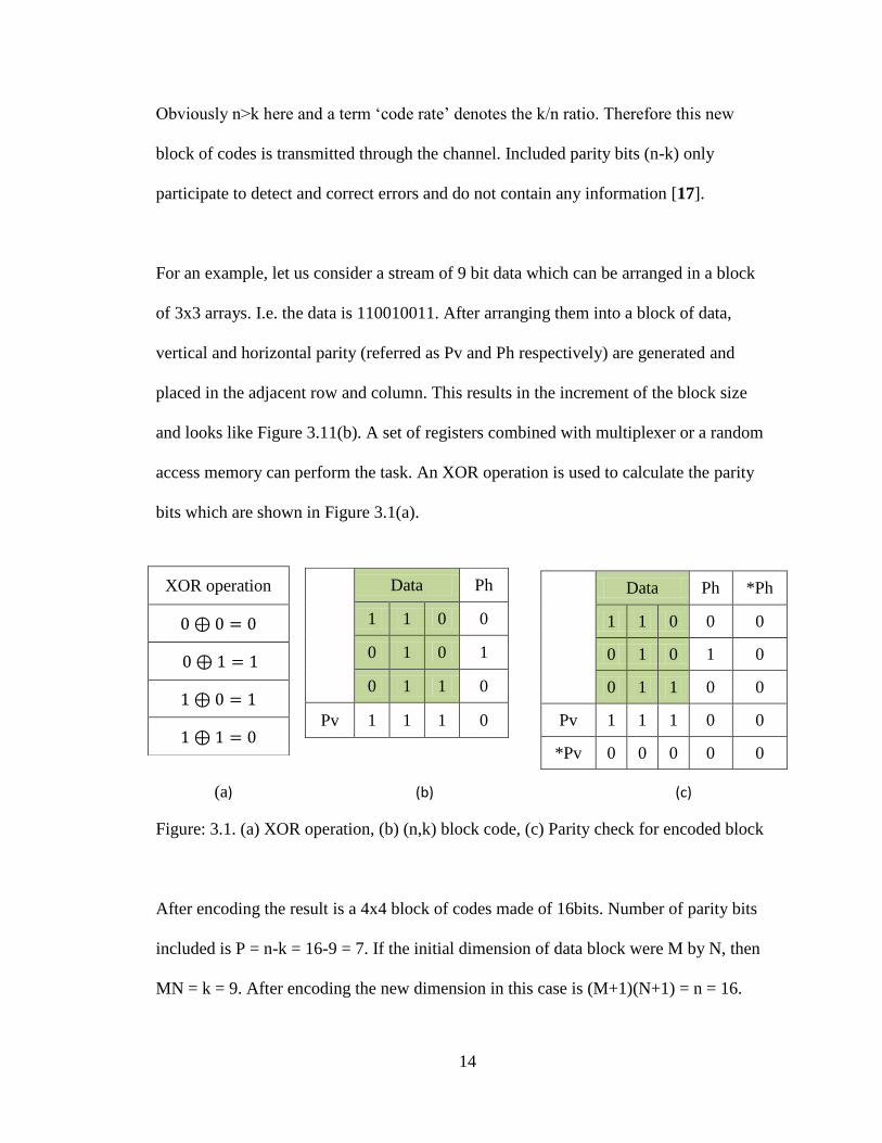
For an example, let us consider a stream of 9 bit data which can be arranged in a block

of 3x3 arrays. I.e. the data is 110010011. After arranging them into a block of data,

vertical and horizontal parity (referred as Pv and Ph respectively) are generated and

placed in the adjacent row and column. This results in the increment of the block size

and looks like Figure 3.11(b). A set of registers combined with multiplexer or a random

access memory can perform the task. An XOR operation is used to calculate the parity

bits which are shown in Figure 3.1(a).

(a) (b) (c)

Figure: 3.1. (a) XOR operation, (b) (n,k) block code, (c) Parity check for encoded block

After encoding the result is a 4x4 block of codes made of 16bits. Number of parity bits

included is P = n-k = 16-9 = 7. If the initial dimension of data block were M by N, then

MN = k = 9. After encoding the new dimension in this case is (M+1)(N+1) = n = 16.

XOR operation

Data Ph

1 1 0 0

0 1 0 1

0 1 1 0

Pv 1 1 1 0

Data Ph *Ph

1 1 0 0 0

0 1 0 1 0

0 1 1 0 0

Pv 1 1 1 0 0

*Pv 0 0 0 0 0

15

So the calculated coding rate is

( )( )

(3.1)

Receiver of this encoded block generates new horizontal parity *Ph and a new vertical

parity *Pv which are shown in Figure 3.1(c). If the there was an error introduced during

the transmission, these bits work to detect and correct the error. Occurrence of error

will result parity check failure at the respective column and row and will show 1

instead of 0. The following figure explains it more.

(a) (b)

Figure: 3.2: (a) Encoded block, (b) Error correction by parity bits

It is shown from the Figure 3.2 (b) that if an error was there in the data it would

generate parity bits in the respective row and column and the receiver will be able to

locate the position of error and can correct it.

Pros and Cons: In case of block codes the receiver can locate the error easily and can

correct it. But if the noise in the channel is too high, it may not be a very effective

scheme. This method can only correct a single bit error in the block. If there is more than

Data Ph *Ph

1 1 0 0 0

0 0 0 1 1

0 1 1 0 0

Pv 1 1 1 0 0

*Pv 0 1 0 0 0

Data Ph

1 1 0 0

0 1 0 1

0 1 1 0

Pv 1 1 1 0

16

one error, it fails to work. More over adding redundant bits grows the volume of the data

which costs bandwidth.

If we consider a block of M-rows and N-columns, the number of information bits D is

given by, (3.2)

After the encoding, ( ) ( ) (3.3)

Where P is the number of parity bits appended to the block.

(3.3)

Table 3.1 below shows how the number of parity bits increases with the size of the

block.

Table: 3.1 Parity bits estimation.

M (Bits) N (Bits) P (Bits)

4 4 9

8 8 17

16 16 33

32 32 65

For a block of 32x32 bits, 65 parity bits are generated and attached to correct a single

error. No information are carried by those additional bits and only used for error

correction. This causes more bandwidth occupation and sometimes slower transmission

over a noisy channel. Optimizing the channel and making it more efficient is always a

challenge improved coding techniques are required to make it better. The project in this

thesis is the investigation of finding a reliable error control solution using orthogonal

codes.

17

3.7 Orthogonal codes

In communication systems, Orthogonal codes like Walsh codes are used for long time as

spreading codes. Besides as spreading codes, it also serves as forward error control (FEC)

code [18]. Systematic block codes like Walsh codes have been proven to be more

efficient and reliable as it is capable to correct more than one error. If an n-bit orthogonal

code is chosen, it can detect and correct up to (

) errors. For a comparison with the

last one in the above table, a 64-bit orthogonal code is able to correct up to 15 errors. The

performance of orthogonal code for FEC is not widely investigated [19] [20]. In this

thesis the application of orthogonal code in LASER communication for FEC is

investigated. To the best of our knowledge, this method has not been checked for LASER

so far and can be a very promising error correction technique for optical communication

as higher bandwidth are available. Also different methods have been discussed to propose

even more bandwidth efficient modulation. The experiment uses Amplitude Shift Keying

(ASK) modulation of LASER and a bi-orthogonal mapping for data encoding.

3.8 Decoding of Orthogonal Code and Error Correction

At the receiver, the incoming encoded data is compared to the lookup table that contains

the mapping structure. Upon the closest approximation (if not a 100 percent match which

is the result of error in transmission) corresponding data bits are stored.

If the orthogonal code is n-bit long, it has n/2 1s and n/2 0s. The only exceptions are all

0s and all 1s. Other than those the distance ‘d’ between the codes become d = n/2. In

exceptional cases it is even higher. This distance property helps to detect and correct the

error in the channel [21] [22]. To apply this distance property, a threshold point at the

18

midway between two orthogonal codes is set. The Figure 3.3 below shows the received

code as dotted line falling between to orthogonal codes.

Figure 3.3: Decoding process of orthogonal code [21] [19]

If n is the code length and dth is denoted as the threshold, the relation between can be

expressed as

(3.4)

The threshold falls at the midway between two orthogonal codes and provides the option

to make the correct decision. The received encoded data is accepted as a valid code if the

n-bit comparison yields a good cross correlation value. The correlation process below is

followed when an impaired orthogonally coded data is compared with a couple of n-bit

orthogonal codes.

( ) ∑ ( ) (3.5)

Provided R(x,y) is the cross-correlation function, n = code length, dth = threshold.

Since the threshold is right in the middle between two valid codes, an 1 bit offset is added

to the equation above to avoid ambiguity.

Orthogonal Code 1 X: x1 x2 ……xn

Orthogonal Code 2 Y: y1 y2 …… yn

dth = n/4

dth = n/4

19

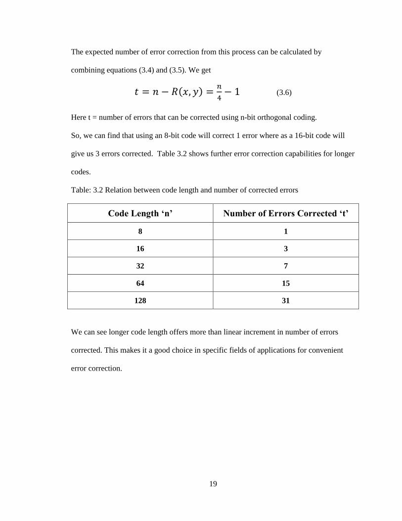
The expected number of error correction from this process can be calculated by

combining equations (3.4) and (3.5). We get

( )

(3.6)

Here t = number of errors that can be corrected using n-bit orthogonal coding.

So, we can find that using an 8-bit code will correct 1 error where as a 16-bit code will

give us 3 errors corrected. Table 3.2 shows further error correction capabilities for longer

codes.

Table: 3.2 Relation between code length and number of corrected errors

Code Length ‘n’ Number of Errors Corrected ‘t’

8 1

16 3

32 7

64 15

128 31

We can see longer code length offers more than linear increment in number of errors

corrected. This makes it a good choice in specific fields of applications for convenient

error correction.

20

CHAPTER 4

ERROR CONTROL AND BANDWIDTH OPTIMIZATION USING

ORTHOGONAL CODE

4.1 Introduction

J. L. Walsh in 1923 developed the aforementioned orthogonal codes. They are also well

known as Walsh codes [23] [19]. Although these codes have been broadly used in Code

Divisional Multiple Access (CDMA) for spreading data, it has been less inquired in other

fields.

Figure 4.1: Expansion of Hadamard Matrix [19] [20]

For orthogonal code generation, Hadamard matrix is the most well- technique. The

following generalized equation is given for the mapping of Walsh sequences [24].

[ ̅̅̅̅

] (4.1)

Figure 4.1. shows the generation of orthogonal code using Hadamard matrix. Any

Hadamard matrix can be generated of order N, when N = 2n (2, 4, 8, 16, 32 . . .).

21

4.2 Properties of Orthogonal Code

Two standalone properties of orthogonal code make them unique as well as a very

efficient for error control coding. These are: Parity generation and Distance properties.

Parity Generation Properties: An orthogonal code in every row generated using

Hadamard matrix has equal number of 1s and 0s in it and the scalar product of the code is

always to be ‘0’. But there is exception as well- when all the bits are 0s or 1s. If the

generated codes are inversed, they are called antipodal codes and they are orthogonal

amongst themselves. That infers an n-bit orthogonal code has an n-bit antipodal code of

its own and all together there is a 2n bi-orthogonal code set. 8 bit orthogonal code set and

the antipodal codes are shown in the Table 4.1

Table: 4.1 n = 8 bit orthogonal and antipodal codes

Antipodal Codes: Inverted regular orthogonal codes produce antipodal codes and possess

the same properties. These codes can be generated in hardware level simply by passing

the orthogonal codes through an in inverter buffer like a NOT gate. Orthogonal codes

Orthogonal code

Antipodal Code

0 0 0 0 0 0 0 0 1 1 1 1 1 1 1 1

0 1 0 1 0 1 0 1 1 0 1 0 1 0 1 0

0 0 1 1 0 0 1 1 1 1 0 0 1 1 0 0

0 1 1 0 0 1 1 0 1 0 0 1 1 0 0 1

0 0 0 0 1 1 1 1 1 1 1 1 0 0 0 0

0 1 0 1 1 0 1 0 1 0 1 0 0 1 0 1

0 0 1 1 1 1 0 0 1 1 0 0 0 0 1 1

0 1 1 0 1 0 0 1 1 0 0 1 0 1 1 0

22

combined with antipodal codes forms the bi-orthogonal matrix which possesses all the

orthogonal properties for all the sequences. Following table shows the set of bi-

orthogonal codes using orthogonal and antipodal codes.

Table 4.2: Bi orthogonal code set by combining Orthogonal and Antipodal codes

Distance Properties: The other property that an orthogonal code set has is the cross

correlation is zero between a pair of them [25]. This relation is given as [21] [22]

( ) ∑ (4.2)

Here two sets of m-bit codes are considered as X1, X2….Xm and Y1, Y2….Ym. In

reality, when the offset between two Walsh code sequences is zero, they show zero cross

correlation between them. The offset can be achieved by synchronization of all the users

of the code which makes it well suitable for CDMA applications [26].

Other properties of orthogonal code include:

Ort

ho

gon

al C

od

e

An

tip

od

al C

od

e

Bi Orthogonal code

23

Data, 2^4 =16 16*8 Mapped result

0000 0000 0000

0001 0101 0101

0010 0011 0011

0011 0110 0110

0100 0000 1111

0101 0101 1010

0110 0011 1100

0111 0110 1001

1000 1111 1111

1001 1010 1010

1010 1100 1100

1011 1001 1001

1100 1111 0000

1101 1010 0101

1110 1100 0011

1111 1001 0110

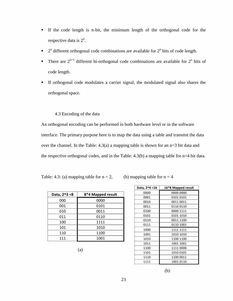
If the code length is n-bit, the minimum length of the orthogonal code for the

respective data is 2n.

2n different orthogonal code combinations are available for 2

n bits of code length.

There are 2n+1

different bi-orthogonal code combinations are available for 2n bits of

code length.

If orthogonal code modulates a carrier signal, the modulated signal also shares the

orthogonal space.

4.3 Encoding of the data

An orthogonal encoding can be performed in both hardware level or in the software

interface. The primary purpose here is to map the data using a table and transmit the data

over the channel. In the Table: 4.3(a) a mapping table is shown for an n=3 bit data and

the respective orthogonal codes, and in the Table: 4.3(b) a mapping table for n=4 bit data.

Table: 4.3: (a) mapping table for n = 2, (b) mapping table for n = 4

(a)

(b)

Data, 2^3 =8 8*4 Mapped result

000 0000

001 0101

010 0011

011 0110

100 1111

101 1010

110 1100

111 1001

24

These data are mapped using a bi-orthogonal coding scheme. For higher values of n, the

table expands accordingly. For the fulfillment of the experiment, mapping table for n = 4,

5, 6 and 7 are generated and used for generating coded data.

The code rate for this orthogonal code is calculated as:

(4.3)

Where r = code rate, and n = number of bits

4.4 Preparation of test bed

The experimental setup features a transmitting station and a receiving station which are

two computers here to serve the purpose. The data is transferred using a LASER which is

ASK modulated by the coded data. The audio output and input ports of the computers are

used to send the bits to the laser and receive the signal from the photodetector

respectively. The laser module used here has its own controller circuit and can operate

while a control signal of 3.0-3.5 volt signal is present. To amplify the output signal from

the computer a high frequency amplifier circuit has been introduced to interface the

LASER. This makes sure that it receives the proper voltage level to drive the beam.

The mapping of data, introduction of the errors, receiving the coded data and extracting

the information using the lookup table and calculation of error is performed by a

program. The program is written using MATLAB®.

The flowchart for the program is given below.

25

Flow chart of the transmission end

Figure 4.2: Transmission end steps in flowchart

Select the file to be sent transmitted. The file contains certain amount of data that can be used

for the experiment.

Select from mapping options of 8/16/32/64 bit mapping of the data

Map the data using the orthogonal code table. Generate the coded data.

Introduce error: select the bits to be altered. Alter the bits in mapped data to simulate errors in the

channel.

Select the frequency of sending. The frequency can be chosen in different kHz ranges.

Generate the final mapped data and send those bits to the port to drive the laser.

26

Flowchart of the receiving end

Figure 4.3: Reception end steps in flowchart

Receive all the bits through the port and log

the data.

Match the received bits with the lookup table

and correlate.

Find the closest matches and retrieve the data.

If there is an error, correct it and keep a

record of the corrected errors.

If there are more than one closest match found

and the data is irrecoverable, record that.

Display the result of recovery process including number of corrected errors and irrecoverable errors.

27

4.5 Bandwidth Optimization

While using Bi-Orthogonal coding, there is a lot of room for bandwidth optimization.

The dimension of the bi orthogonal code depends on the mapping sequence of input data

bits. It follows the equation:

(4.4)

Where n = number of bits and K*K/2 is the dimension of the bi-orthogonal matrix

required for the data mapping

The Table 4.4 explains how the expansion of bi-orthogonal matrix moves with respect to

number of bits:

Table 4.4: Expansion of bi-orthogonal matrix size respect to number of bits

Number of bits Number of combinations Bi orthogonal matrix

3 2^3=8 8*4

4 2^4=16 16*8

5 2^5=32 32*16

6 2^6=64 64*32

7 2^7=128 128*64

8 2^8=256 256*128

It is visible from the table that the requirement of the bigger matrix size of the bi

orthogonal coding increases exponentially. This costs lots of bandwidth in this case. But

it can be significantly reduced by bit splitting.

28

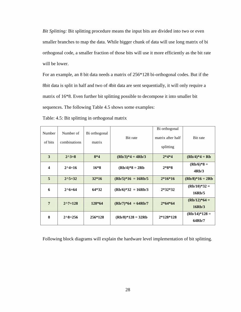
Bit Splitting: Bit splitting procedure means the input bits are divided into two or even

smaller branches to map the data. While bigger chunk of data will use long matrix of bi

orthogonal code, a smaller fraction of those bits will use it more efficiently as the bit rate

will be lower.

For an example, an 8 bit data needs a matrix of 256*128 bi-orthogonal codes. But if the

8bit data is split in half and two of 4bit data are sent sequentially, it will only require a

matrix of 16*8. Even further bit splitting possible to decompose it into smaller bit

sequences. The following Table 4.5 shows some examples:

Table: 4.5: Bit splitting in orthogonal matrix

Number

of bits

Number of

combinations

Bi orthogonal

matrix

Bit rate

Bi orthogonal

matrix after half

splitting

Bit rate

3 2^3=8 8*4 (Rb/3)*4 = 4Rb/3 2*4*4 (Rb/4)*4 = Rb

4 2^4=16 16*8 (Rb/4)*8 = 2Rb 2*8*8 (Rb/6)*8 =

4Rb/3

5 2^5=32 32*16 (Rb/5)*16 = 16Rb/5 2*16*16 (Rb/8)*16 = 2Rb

6 2^6=64 64*32 (Rb/6)*32 = 16Rb/3 2*32*32 (Rb/10)*32 =

16Rb/5

7 2^7=128 128*64 (Rb/7)*64 = 64Rb/7 2*64*64 (Rb/12)*64 =

16Rb/3

8 2^8=256 256*128 (Rb/8)*128 = 32Rb 2*128*128 (Rb/14)*128 =

64Rb/7

Following block diagrams will explain the hardware level implementation of bit splitting.

29

In the following Figure 4.2, we can see the Code rate r=1/2, Transmit bit rate = 2Rb,

Bandwidth BW = 2*2Rb = 4Rb Hz

Figure: 4.4 Bit Splitting, 4-bit input and 16x8 mapping

When 16 bit inputs are split into two 8 bit inputs, the change is shown in the following

Figure 4.3. Here Code rate r=3/4, Transmit bit rate = 4Rb/3, Bandwidth BW = 2*4Rb/3

Rb = 8Rb/3 Hz

Figure: 4.5 Bit Splitting, 2*3-bit input and 2*(8x8) mapping

16

*8 R

OM

4 t

o 1

6 D

eco

der

1:4 Serial to

parallel converter

Data in, R

b

Rb/4

(Rb/4)*8 = 2R

b

fc

To LASER

8*8

ROM 3 t

o 8

D

eco

der

1:6 Serial to parallel convert

er

Data in, R

b

Rb/6 (R

b/6)*8 = 4R

b/3

fc

To LASER

8*8

ROM 3 t

o 8

D

eco

der

30

After splitting further, the fixture would look like the one in the Figure 4.4. Here Code

rate r=1, Transmit bit rate = Rb, Bandwidth BW = 2*Rb = 2Rb Hz

Figure: 4.6 Bit Splitting, 4*2-bit input and 4*(4x8) mapping

Error control and bandwidth optimization options are two major advantages of

Orthogonal coding schemes. In LASER communication, the orthogonal coding

performance is verified using On-Off Keying modulation and experiments and results are

discussed in the following chapter.

4*8

ROM

1:8 Serial to parallel convert

er

Data in, R

b

(Rb/8)*8 = R

b

fc

To LASER

4*8

ROM 2 t

o 4

D

eco

der

Rb/8

2 t

o 4

D

eco

der

4*8

ROM

4*8

ROM 2 t

o 4

D

eco

der

2 t

o 4

D

eco

der

31

CHAPTER 5

EXPERIMENTAL RESULT

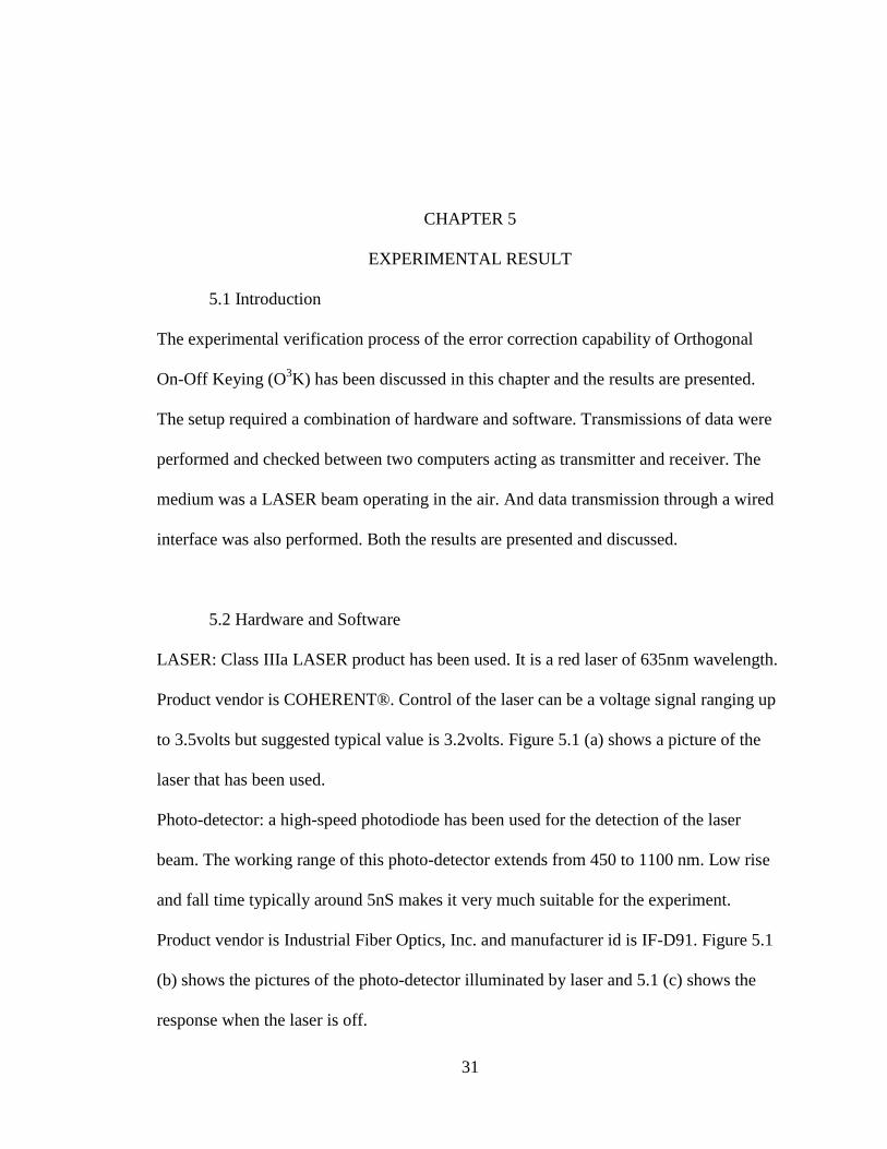
5.1 Introduction

The experimental verification process of the error correction capability of Orthogonal

On-Off Keying (O3K) has been discussed in this chapter and the results are presented.

The setup required a combination of hardware and software. Transmissions of data were

performed and checked between two computers acting as transmitter and receiver. The

medium was a LASER beam operating in the air. And data transmission through a wired

interface was also performed. Both the results are presented and discussed.

5.2 Hardware and Software

LASER: Class IIIa LASER product has been used. It is a red laser of 635nm wavelength.

Product vendor is COHERENT®. Control of the laser can be a voltage signal ranging up

to 3.5volts but suggested typical value is 3.2volts. Figure 5.1 (a) shows a picture of the

laser that has been used.

Photo-detector: a high-speed photodiode has been used for the detection of the laser

beam. The working range of this photo-detector extends from 450 to 1100 nm. Low rise

and fall time typically around 5nS makes it very much suitable for the experiment.

Product vendor is Industrial Fiber Optics, Inc. and manufacturer id is IF-D91. Figure 5.1

(b) shows the pictures of the photo-detector illuminated by laser and 5.1 (c) shows the

response when the laser is off.

32

Transceiver computers: Any computer that is capable to run MATLAB® R2012a or

R2010a is good to work as the transmitter or receiver end of the experiment. These two

versions of MATLAB® are confirmed to perform as it has been tested. But other

versions are expected to support as well.

Signal amplifier: A TL071 high frequency operational amplifier was used for the

amplification of the signal. Received signal is magnified to the required level, here in this

case signal raised to 3.2 volts to drive the laser.

Software: Programming Language: MATLABTM

2012a used to prepare the software.

Audio software: Audacity 2.0.5 and Windows Media Player are used to record the

received data and send the data to laser by playing the audio file respectively.

Figure: 5.1(a) LASER for data transmission

Figure: 5.1(b) Photo-detector (LASER on) Figure: 5.1(c) Photo-detector (LASER off)

33

5.3 Construction of the Experiment

The purpose of the whole experiment in this project to test the orthogonal coding scheme

applied to a set of data that is transferred through a laser channel. The channel attenuation

and noise can interfere with the data transfer and create error in the bits. For the

experimental purpose, random bits were altered to simulate the error in the channel. The

receiver end will log the data bits and use the mapping table for correction and confirm

the performance orthogonal codes in forward error correction. The expected error

correction ability is given by the following equation

⁄ (5.1)

Where t = number of errors corrected and n = number of bits

Table 5.1 shows the number of error correction for n = 8, 16, 32, 64

Table: 5.1 Percentage of error correction and code length

Code Length ‘n’ Number of Errors Corrected ‘t’ Percentage or error correction

8 1 12.50%

16 3 18.75%

32 7 21.87%

64 15 23.43%

5.3.1 Selection of data file: At first, a file is prepared to send over the channel and

because it is an experiment the number of the bits in the file has been selected carefully to

suite the program written in MATLAB®. For this, a common multiple of selected n

values (4,5,6,7) were taken and that many number of bits were placed in the file to make

sure the program can map all the bits inside. If not a multiple of the given n values, the

program will have unmatched size of array and will not proceed.

34

5.3.2 Mapping of the data: There have been options created to map the data for four

different lengths of the bi-orthogonal code, which are 8, 16, 32 and 64 bits. Upon the

choice of the user, any mapping option can be selected. The higher dimension of the

mapping table is chosen, the more correction of error is possible. But it will increase the

volume of the mapped result as well.

5.3.3 Introduction of errors: To simulate the errors in the channel, the program is

prepared to introduce errors in the bit stream. User can choose any number of errors to be

in the file from zero to all. Selected bits will be altered from the generated orthogonally

coded data. For an example, altering 16 bits in every 64 bits will result creating 25% of

error in the data. Both the numbers are variable and can be chosen independently. Such

as, it can be chosen to be 2 bits out of every 16 bits. If no error to be introduced, simply

putting 0 out of every 16 bits will do it.

5.3.4 Choice of bit rate: The user can choose the frequency at which the data will be sent

out. This forms the bit rate of the transmission.

5.3.5 Conversion into wave file: Last step of the program is to convert the binary file into

a wave file also known as wav file format. Because in this file format data is stored in

linear pulse coded modulation, the data bit stream of 0s and 1s become discrete voltage

levels in the time domain. This file can be executed from any audio player software.

35

5.3.6 Sending out the bits: The bits are sent out simply by playing the wav file. Any audio

playing software can do that. In this experiment the Windows Media Player has been

used. From the audio output port of the computer the bit stream will be available as the

wave file executed.

5.3.7 Amplification: As the audio port gives away the signal of our interest, it is fed into

the amplifier circuit. A high frequency operational amplifier performs the amplification

and raises the peak voltage up to 3.2 volts.

5.3.8 Operation of laser: The output signal of the amplifier has two discrete levels to

denote 0 and 1. For 0 the voltage level is ~0volt and for 1, it is ~3.2 volts. The control

input of the laser is directly connected to the output of the amplifier. The On operation of

the laser takes place between the ranges of 3.0-3.5volts. So, the laser is On-Off

modulated by the 0s and 1s of the data file created earlier.

5.3.9 Detection and logging of the signal: LASER beam is pointed at the photodetector

and generates responses according to the laser illumination. The signal produces a

response of ~400mV when fully brightened by the laser and ~0volt when no beam is

falling upon its lens. This range of voltage is adequate for the detection of bits. So as a

result a stream of data bits is produced from the terminals of the photodetector. This

signal is fed into the ‘line in’ audio recording port of the receiver end computer.

36

5.3.10 Recording of the data: The line in audio port of is typically used to collect and

record signals from audio sources. It is capable to collect and store the change in the

voltage of a source in time domain. So this option has been used here to record all the

signals and analyze later one. The software Audacity 2.0.5 has been used to record the

reception and store it as a wav file.

5.3.11 Data retrieval and error correction: The recorded wav file contains the received

bits in the time domain. 0s and 1s are represented as the ~0Volt and ~400mVolt

respectively. The receiver part of the MATLAB® program now analyzes the file and

determines the bits using a threshold value. After recognition of the bits, it is matched

with the lookup table. User can define which lookup table to be used here and can select

from the 8, 16, 32 or 64bit options to check. Upon correct selection, the program will

pick bits from the file and match with the lookup table. When a perfect match is found, it

will store the respective data bits as the retrieved data. If it is not matched all the way

along the length of the data, the closest matches are picked for analysis.

Mismatched bits in the code length are counted as errors in the transmission. If the

number of errors in the transmission falls in the range of error correction ability of the

coding, there should be only one closest match to any one of the rows in the lookup table.

For an example, if 10 error bits were found in a 64 bit long code, in the lookup table there

should be only one match that is closest to the bits received. On the other hand, if there

are 16 or more errors found in a 64bit long code, there will be more than one closest

match in the lookup table. In that case, the program will be unable to correct the number

of errors as more than one match is found say it is 3 or 4 matches. There is no way to

37

confirm which one is the right match. But if it falls in the range of correctable number of

errors, it will take the closest match and correct it. Will record the number of corrected

bits as well, retrieve the data and display the result.

For the experiment, multiple combinations of mapping table along with the numbers of

introduced errors and the rate of transmission were checked. Various permutations and

combinations using all the parameters were tried over the channel using laser and wired

transmission. All the results are collected and used for the verification of the error

correction ability of the coding.

The following figures from Figure 5.2 to Figure 5.9 show the pattern of transmitted and

received data by LASER and wired transmission. All the responses show the signal

transmitted and received in time domain. Each section includes the transmission bits and

reception signals by laser as well as wired interface. The responses are properly aligned

to compare between the same bits for transmission and reception.

38

5.3.12 Visual pattern of the 8 bit mapped transmission and reception

Figure: 5.2 (a): 8 bit mapping, 1 error in every 8 bit, 4 kHz transmission

Figure: 5.2 (b): 8 bit mapping, 2 errors in every 8 bit, 4 kHz transmission

Figure: 5.3 (a): 8 bit mapping, 1 error in every 8 bit, 8 kHz transmission


Transmission bits

Transmission bits

Transmission bits

Transmission bits

LASER reception

Wired reception

LASER reception

Wired reception

LASER reception

Wired reception

LASER reception

Wired reception

39


Figure: 5.4 (a): 16 bit mapping, 3 errors in every 16 bit, 4 kHz transmission




Transmission bits

Wired reception

LASER reception

Transmission bits

Wired reception

LASER reception

Transmission bits

Wired reception

LASER reception

Transmission bits

Wired reception

LASER reception

40






Transmission bits

Wired reception

LASER reception

Transmission bits

Wired reception

LASER reception

Transmission bits

Wired reception

LASER reception

Transmission bits

Wired reception

LASER reception

41






Transmission bits

Wired reception

LASER reception

Transmission bits

Wired reception

LASER reception

Transmission bits

Wired reception

LASER reception

Transmission bits

Wired reception

LASER reception

42

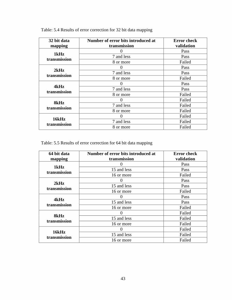
5.3.16 Summary of LASER reception results: The following tables show the performance

of error correction over various different combinations for LASER reception.

Table: 5.2 Results of error correction for 8 bit data mapping

8 bit data

mapping

Number of error bits introduced at

transmission

Error check

validation

1kHz

transmission

0 Pass

1 Pass

2 or more Failed

2 kHz

transmission

0 Pass

1 Pass

2 or more Failed

4 kHz

transmission

0 Pass

1 Pass

2 or more Failed

8kHz

transmission

0 Failed

1 Failed

2 or more Failed

16kHz

transmission

0 Failed

1 Failed

2 or more Failed


16 bit data

mapping


transmission

Error check

validation

1kHz

transmission

0 Pass

3 and less Pass

4 or more Failed

2kHz

transmission

0 Pass

3 and less Pass

4 or more Failed

4kHz

transmission

0 Pass

3 and less Pass

4 or more Failed

8kHz

transmission

0 Failed

3 and less Failed

4 or more Failed

16kHz

transmission

0 Failed

3 and less Failed

4 or more Failed

43


32 bit data

mapping


transmission

Error check

validation

1kHz

transmission

0 Pass

7 and less Pass

8 or more Failed

2kHz

transmission

0 Pass

7 and less Pass

8 or more Failed

4kHz

transmission

0 Pass

7 and less Pass

8 or more Failed

8kHz

transmission

0 Failed

7 and less Failed

8 or more Failed

16kHz

transmission

0 Failed

7 and less Failed

8 or more Failed


64 bit data

mapping


transmission

Error check

validation

1kHz

transmission

0 Pass

15 and less Pass

16 or more Failed

2kHz

transmission

0 Pass

15 and less Pass

16 or more Failed

4kHz

transmission

0 Pass

15 and less Pass

16 or more Failed

8kHz

transmission

0 Failed

15 and less Failed

16 or more Failed

16kHz

transmission

0 Failed

15 and less Failed

16 or more Failed

44

5.3.17 Summary of wired reception results: The following tables show the performance

of error correction over many different combinations for Wired Reception.


8 bit data

mapping


transmission

Error check

validation

1kHz

transmission

0 Pass

1 Pass

2 or more Failed

2 kHz

transmission

0 Pass

1 Pass

2 or more Failed

4 kHz

transmission

0 Pass

1 Pass

2 or more Failed

8kHz

transmission

0 Pass

1 Pass

2 or more Failed

16kHz

transmission

0 Failed

1 Failed

2 or more Failed


16 bit data

mapping


transmission

Error check

validation

1kHz

transmission

0 Pass

3 and less Pass

4 or more Failed

2kHz

transmission

0 Pass

3 and less Pass

4 or more Failed

4kHz

transmission

0 Pass

3 and less Pass

4 or more Failed

8kHz

transmission

0 Pass

3 and less Pass

4 or more Failed

16kHz

transmission

0 Failed

3 and less Failed

4 or more Failed

45


32 bit data

mapping


transmission

Error check

validation

1kHz

transmission

0 Pass

7 and less Pass

8 or more Failed

2kHz

transmission

0 Pass

7 and less Pass

8 or more Failed

4kHz

transmission

0 Pass

7 and less Pass

8 or more Failed

8kHz

transmission

0 Pass

7 and less Pass

8 or more Failed

16kHz

transmission

0 Failed

7 and less Failed

8 or more Failed


64 bit data

mapping


transmission

Error check

validation

1kHz

transmission

0 Pass

15 and less Pass

16 or more Failed

2kHz

transmission

0 Pass

15 and less Pass

16 or more Failed

4kHz

transmission

0 Pass

15 and less Pass

16 or more Failed

8kHz

transmission

0 Pass

15 and less Pass

16 or more Failed

16kHz

transmission

0 Failed

15 and less Failed

16 or more Failed

46

From Table 5.2 to Table 5.9 above it is shown that the performance of the Orthogonal

On-Off keying for error correction is well acquired by the LASER and wired

transmission. However wired transmission shows better performance in higher frequency

than the LASER. This helps to understand the required hardware support for driving the

laser and detection of a high frequency signal. In case of higher frequency the recording

of the received signal may not be as optimized as well as the low frequency modulation.

This is quite visible from the pattern of the received signals. Filtration and noise

cancelation circuits may also come in effect inside the hardware which also may cause

poor reception at higher frequency. That is why the program was able to correct the errors

in laser reception at around 4 kHz and less but as the frequency went higher, the

reception went poor. Weak reception and noise in the channel attenuated the signal below

the selected threshold at points and program failed to detect the bits properly. However

wired transmission showed better performances in this regard and showed expected error

correction results around 8kHz transmission. But above that it failed as well. The visual

patterns show the comparison between bits received by LASER and wired transmission

and the difference between lower and higher frequency. To study the higher frequency

response beyond this range, some hardware modification and equipment recommendation

are also discussed in the following chapter.

5.4 Bit Error Rate and performance analysis

In data transmission, number of error bits are counted as the number of bits altered in the

channel. This change in the bits can be a result of the noise, interference, defects,

distortions or other unwanted parameters. The calculation of Bit Error Rate (BER) refers

47

to the ratio of number of error bits to the number of bits transferred during a certain time

period. The study of bit error rate analysis helps to analyze the performance of error

control coding in a certain channel.

The expected value of bit error rate is referred as bit error probability Pe. Thus the BER

gives an approximate estimation of error occurrence. As mentioned earlier, there are

numbers of factors in the channel that can cause errors. Calculation of BER and Coding

Gain will complement the study.

Coding gain: For uncoded data, if there is an error it cannot be corrected. On the other

hand coded data transmission comes into play to provide error correction. Coding gain is

obtained by comparing the BER with coding to the BER without coding. Measurement of

coding gain helps to understand the performances between different codes as well as

uncoded data.

For the bit error rate calculation a channel model is introduced to simulate the random

noise in the transmission. Additive White Gaussian Noise (AWGN) is a channel model

and it is used to mimic the random processes in nature. Additive- refers that it is added to

any noise intrinsical to the system. White refers to that it considers uniform noise power

distribution. And it is Gaussian because the normal distribution in the time domain yields

an average value of zero.

Now, for the uncoded data, the bit error rate expression is [2] [27].

( )

(√ ⁄ ) (5.2)

And, for the coded data, the bit error rate expression is [2] [27].

( ) ∑ ( )

( ) ( ( ) )

(5.3)

48

Here AWGN stands for Additive White Gaussian Noise. If we plot the results for

orthogonally mapped data using the equations above, we find the following.

Figure: 5.10 BER performances for 8/16/32/64/128/256/512 bit bi-orthogonal codes- wide scale view

Figure: 5.11 BER performances for 8/16/32/64/128/256/512 bit bi-orthogonal code- zoomed view.

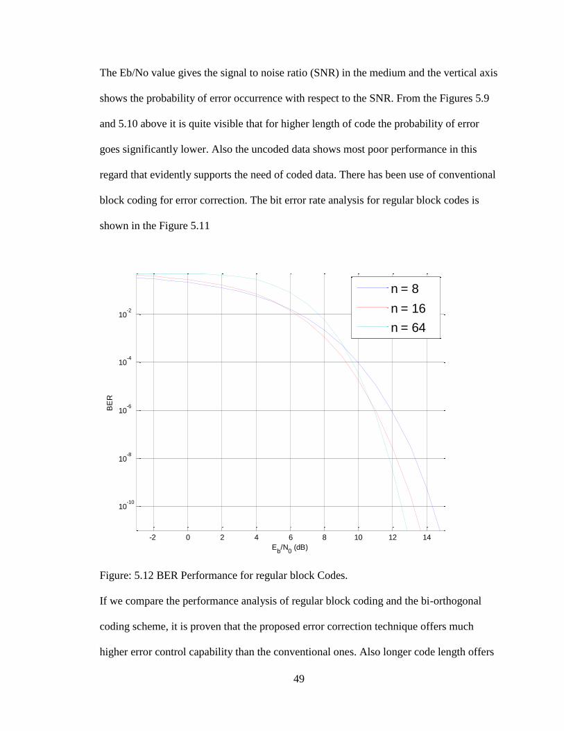
49

The Eb/No value gives the signal to noise ratio (SNR) in the medium and the vertical axis

shows the probability of error occurrence with respect to the SNR. From the Figures 5.9

and 5.10 above it is quite visible that for higher length of code the probability of error

goes significantly lower. Also the uncoded data shows most poor performance in this

regard that evidently supports the need of coded data. There has been use of conventional

block coding for error correction. The bit error rate analysis for regular block codes is

shown in the Figure 5.11

Figure: 5.12 BER Performance for regular block Codes.

If we compare the performance analysis of regular block coding and the bi-orthogonal

coding scheme, it is proven that the proposed error correction technique offers much

higher error control capability than the conventional ones. Also longer code length offers

-2 0 2 4 6 8 10 12 14

10-10

10-8

10-6

10-4

10-2

Eb/N

0 (dB)

BE

R

Bit error probability curve of Orthogonal codes for BPSK modulation

n = 8

n = 16

n = 64

50

higher coding gain which allows choosing the suitable block size for coding in a certain

channel.

Code rate performance of Orthogonal and Bi-orthogonal coding: Orthogonal coding has

been used in Code Divisional Multiple Access (CDMA) communication as an error

control coding. But using a set of bi-orthogonal matrix for error control is a new idea for

laser communication. As mentioned earlier, every block of orthogonal codes has a set of

antipodal codes and antipodal codes are orthogonal amongst themselves as well. These

two sets of blocks combined, forms the bi orthogonal code matrix and the following

analysis shows the difference in the code rate of orthogonal and bi-orthogonal coding.

For orthogonal codes, the coding rate r is given by

(5.4)

For bi-orthogonal codes, the coding rate r is given by

(5.5)

Combining the two Equations (5.4) and (5.5) above, we can calculate the percentage of

increment in coding rate. That shows

(5.6)

It is obvious that using bi-orthogonal code will give the option to encode twice the

number of data combinations. For an example, if n = 3, length of orthogonal code length

has to be 8, whereas length of bi-orthogonal code will only be 4. For n = 4, orthogonal

and bi-orthogonal code lengths are 16 and 8 respectively. So, the increment in code rate

remains same for the same value of n. The Table 5.10 shows more examples of it.

51

But the change in bi orthogonal code rate with respect to the increment of bit number and

consequently larger code length is more of an interesting phenomenon.

Table: 5.10 Change in code rate calculation

Number

of bits ‘n’

Orthogonal

code length

Bi-

orthogonal

code

length

Orthogonal

code rate

Bi-

orthogonal

code rate

Increase

in code

rate

Bi-orthogonal

code rate

increment

compared to

orthogonal

coding

3 8 4 0.3750 0.7500 50.00% 33.333%

4 16 8 0.2500 0.5000 50.00% 25.000%

5 32 16 0.1563 0.3125 50.00% 20.000%

6 64 32 0.0938 0.1875 50.00% 16.667%

7 128 64 0.0547 0.1094 50.00% 14.286%

8 256 128 0.0313 0.0625 50.00% 12.500%

9 512 256 0.0176 0.0352 50.00% 11.111%

10 1024 512 0.0098 0.0195 50.00% 10.000%

11 2048 1024 0.0054 0.0107 50.00% 9.091%

12 4096 2048 0.0029 0.0059 50.00% 8.333%

13 8192 4096 0.0016 0.0032 50.00% 7.692%

14 16384 8192 0.0009 0.0017 50.00% 7.143%

15 32768 16384 0.0005 0.0009 50.00% 6.667%

Due to different values of n, different code length is required. Different code lengths

exert different code rates. Above from the Table 5.10, we can see how the code rate

changes between orthogonal and bi-orthogonal coding while value of n is varied.

From the numbers, we can see that the decrement in the percentage of code rate follows a

nonlinear pattern. Higher code rate is always desired for more efficient data transmission

while using error control coding. And we can see for all the cases, bi-orthogonal code

rate is higher than the orthogonal coding which is an advantage over the existing scheme.

For higher values of n- which also indicates longer bi orthogonal code, the change in

52

code rate decreases gradually. The change is plotted in the Figure 5.12 below. The plot

shows the code rate performance of bi orthogonal mapping for different code lengths.

Figure: 5.13 Change in code rate for different code lengths of bi-orthogonal mapping

From the Figure 5.12 we can see that if the code length becomes 512 or longer, the

difference between orthogonal and bi orthogonal code rate becomes smaller and smaller.

This describes the difference between them in longer codes and helps to choose the

length of the code accordingly.

Point of diminishing return: Another parameter to choose the correct length of coding

depends on the performance or error correction in different code lengths. The error

correction capability increases with the length of the code but this increment is not linear

either. To see the changes in error correction performance the following Table 5.11 is

populated using the Equation 5.1 for n = 2 to 15.

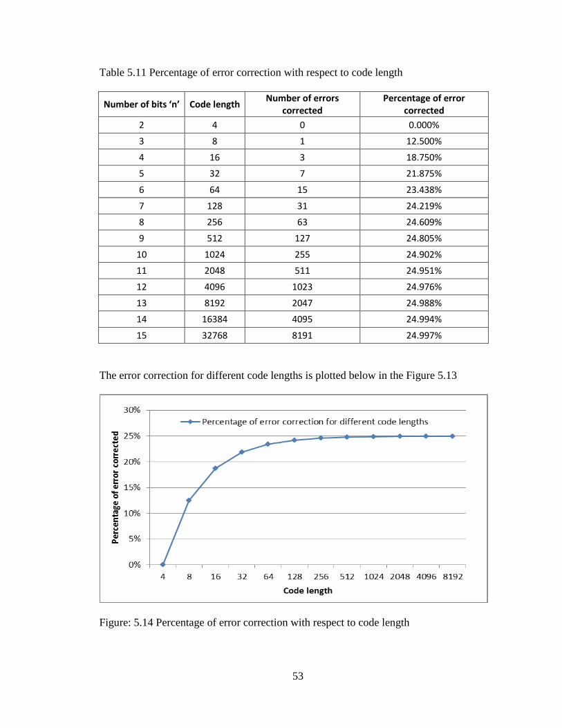
53

Table 5.11 Percentage of error correction with respect to code length

Number of bits ‘n’ Code length Number of errors

corrected Percentage of error

corrected

2 4 0 0.000%

3 8 1 12.500%

4 16 3 18.750%

5 32 7 21.875%

6 64 15 23.438%

7 128 31 24.219%

8 256 63 24.609%

9 512 127 24.805%

10 1024 255 24.902%

11 2048 511 24.951%

12 4096 1023 24.976%

13 8192 2047 24.988%

14 16384 4095 24.994%

15 32768 8191 24.997%

The error correction for different code lengths is plotted below in the Figure 5.13

Figure: 5.14 Percentage of error correction with respect to code length

54

From the Figure 5.13, we can see the error correction capability almost saturates after 256

bit code length. Longer code than 256 bit offers error correction towards 25% but at the

cost of a much higher bit rate. To find out more efficient error correction in terms of code

length we can check the length varying from 8 to 128 bit. This part of the plot shows

error correction ranging from 12.5% to 24.22%. Looking at the pattern of the plot we can

tell the most efficient error control coding considering the code length can be expected

from 16, 32 or 64 bit coding. Depending on the channel characteristics and application, a

suitable mapping option can be obtained from the above mentioned analysis.

Considering the bit error rate performance, coding gain, code rate and option for

bandwidth optimization, the Orthogonal On-Off Keying shows very high potential in

laser communication and promising error control performance in practice. In addition,

this coding scheme can also be applied to other modulation technique.

55

CHAPTER 6

FUTURE WORK AND CONCLUSION

LASER communication is an alternative solution over RF communication for long-haul

connectivity and security. And Orthogonal On-Off Keying can be a complementary error

control coding scheme to that approach. The higher error correction capability, self-

synchronization property, lower implementation cost, easy maintenance and other

characteristics make it a promising alternative in the future of communication systems.

However, there are many challenges on the way before it can be applied and be available

for mass use. This requires further research and development and leaves a lot of room for

future works.

In this thesis, the direct modulation of laser using orthogonal codes has been investigated.

The sub carrier modulation and other modulation techniques can be applied and may

provide even greater bandwidth efficiency. Analog modulations like amplitude

modulation (AM), frequency modulation (FM) or pulse modulation (PM) and digital

modulations like Frequency Shift Keying (FSK), Phase Shift Keying (PSK) or Pulse

Position Modulation (PPM) can be lucrative topics of research.

In the current experiment the upper limit of the frequency to check the response was

limited. To extend this to higher frequencies and study the response some hardware

modification will help. Use of a Data Acquisition System like Signatec or Pico

56

Technology product for data acquisition may help to capture higher frequency receiving

signal. Switching to high speed LASER product and PIN diode for detection will increase

the bandwidth. Also, the Universal Serial Bus (USB) port instead of the audio interface

can be used here and in that case the port itself can detect high speed signals. As for an

example if a USB 3.0 is used, it can respond up to 5 gigabits per second and will give

acceptance of a lot higher frequency range. USB 2.0 interface is fairly low compared to

that and has the limit of going up to 480 megabits per second but that can be used too for

experiments in that range [28]. The program will need to include configuration of USB

port in this regard to perform the tasks.

For detection of LASER the bright ambient light in day time can be a challenge for good

reception. There needs to be a reliable means of receiver for detection in all conditions.

Differential receiver can be a potential solution which needs further research and

development.

Successful communication using laser depends largely on proper alignment of the beam

towards the photodetector. Manual adjustment may not be a well suited option for long

distance coverage and development to an automated alignment system is demanding. A

retro reflector alignment system can be considered for future development in this regard.

The prospect of laser based communication system is very high and with secured high

speed data transfer ability, it has already proved its potential. Any line of sight

communication ranging from air to air, ground to ground, air to ground, space to ground,

deep space communication or even for underwater communication, this is a promising

57

solution. With proper development and implementation of error controlling capacity like

orthogonal coding and combining with different modulation techniques it can provide

higher speed data access to mass user.

APPENDICES

59

Appendix A

Appendix A contains the steps of the experiment.

Preparation of the transmitter

Connect a stereo jack to the audio output port of the transmitter computer

Connect the left or right channel output to the amplifier input

Connect the amplifier output to the laser control input

All the grounds to be connected

Open MATLAB® in the computer

Run the file final_t8/16/32/64 for 8/16/32 or 64 bit mapping respectively

Use the parameters “inputdata” for input file, “f” for frequency, “err” for number of

errors to be introduced and “eml” to define the window of bits to choose ‘err’ from

Running the file will create a wav file named Tx.wav in the same folder

Playing the wav file will send the bits out to the laser to drive

Preparation of the receiver

Connect photodiode to the left channel of ‘Line in’ audio port of the receiver computer

Select the ‘Line in’ as the recording option in Audacity and start recording

Experiment

Play the Tx.wav file. It will modulate the laser and the response will be recorded by

Audacity software in the receiver computer. Save the recorded file in wav format.

Run final_r8/16/32/64 (same as transmitted one) to check the received file.

60

Appendix B

Appendix A contains the MATLAB® code for 8bit data mapping of a binary input file

with the choice of number of errors to introduce and bit rate. This also converts the

mapped data into a file.

function out_t = final_t8(inputdata,f,err,eml)

i=1; j=1;

for i=1:4:length(inputdata)

if (inputdata(i:i+3) == [0 0 0 0]) out(j:j+7) = [0 0 0 0 0 0 0 0];

elseif(inputdata(i:i+3) == [0 0 0 1]) out(j:j+7) = [0 1 0 1 0 1 0 1];











61




else out(j:j+7) = [1 0 0 1 0 1 1 0]; end

j=j+8;

end

out1=out; out = error_calc(out1,err,eml);

e = [0 0 0 1 0 1 0 1 0 1 0 1 0 0 0 0]; s = [1 1 1 0 1 0 1 0 1 0 1 0 1 1 1 1]; out = [1 1 1 1 1 1 1 1 1 1 1 1 1 1 1 1 s out e e e e];

i=1; t=0; j=1; for i=1:1:length(out) for t=(0+2/f):2/f:1 out_t(j)=out(i)*1; j=j+1; end

end out_t = out_t*1; wavwrite(out_t,44100,16,'Tx');

end

62

Appendix C

Appendix B contains the MATLAB® code for 16 bit data mapping of a binary input file




i=1; j=1;


if (inputdata(i:i+4) == [0 0 0 0 0]) out(j:j+15) = [0 0 0 0 0 0 0 0 0 0 0 0 0 0 0 0];

elseif(inputdata(i:i+4) == [0 0 0 0 1]) out(j:j+15) = [0 1 0 1 0 1 0 1 0 1 0 1 0 1 0 1];










63






elseif (inputdata(i:i+4) == [1 0 0 0 0]) out(j:j+15) = [1 1 1 1 1 1 1 1 1 1 1 1 1 1 1 1];











64





elseif(inputdata(i:i+4) == [1 1 1 1 1]) out(j:j+15) = [1 0 0 1 0 1 1 0 0 1 1 0 1 0 0 1]; else

end

j=j+16;

end

out1=out; out = error_calc(out1,err,eml);

e = [0 0 0 1 0 1 0 1 0 1 0 1 0 0 0 0]; s = [1 1 1 0 1 0 1 0 1 0 1 0 1 1 1 1]; out = [1 1 1 1 1 1 1 1 1 1 1 1 1 1 1 1 s out e e e e];

i=1; t=0; j=1; for i=1:1:length(out) for t=(0+2/f):2/f:1 out_t(j)=out(i)*1; j=j+1; end

end out_t = out_t*1; wavwrite(out_t,44100,16,'Tx');

end

65

Appendix D

Appendix C contains the MATLAB® code for 32 bit data mapping of a binary input file




i=1;

j=1;


if (inputdata(i:i+5) == [0 0 0 0 0 0])

out(j:j+31) = [0 0 0 0 0 0 0 0 0 0 0 0 0 0 0 0 0 0 0 0 0 0 0 0 0 0 0 0 0 0 0 0];

elseif(inputdata(i:i+5) == [0 0 0 0 0 1])

out(j:j+31) = [0 1 0 1 0 1 0 1 0 1 0 1 0 1 0 1 0 1 0 1 0 1 0 1 0 1 0 1 0 1 0 1];


out(j:j+31) = [0 0 1 1 0 0 1 1 0 0 1 1 0 0 1 1 0 0 1 1 0 0 1 1 0 0 1 1 0 0 1 1];


out(j:j+31) = [0 1 1 0 0 1 1 0 0 1 1 0 0 1 1 0 0 1 1 0 0 1 1 0 0 1 1 0 0 1 1 0];


out(j:j+31) = [0 0 0 0 1 1 1 1 0 0 0 0 1 1 1 1 0 0 0 0 1 1 1 1 0 0 0 0 1 1 1 1];


out(j:j+31) = [0 1 0 1 1 0 1 0 0 1 0 1 1 0 1 0 0 1 0 1 1 0 1 0 0 1 0 1 1 0 1 0];


out(j:j+31) = [0 0 1 1 1 1 0 0 0 0 1 1 1 1 0 0 0 0 1 1 1 1 0 0 0 0 1 1 1 1 0 0];


out(j:j+31) = [0 1 1 0 1 0 0 1 0 1 1 0 1 0 0 1 0 1 1 0 1 0 0 1 0 1 1 0 1 0 0 1];


out(j:j+31) = [0 0 0 0 0 0 0 0 1 1 1 1 1 1 1 1 0 0 0 0 0 0 0 0 1 1 1 1 1 1 1 1];


out(j:j+31) = [0 1 0 1 0 1 0 1 1 0 1 0 1 0 1 0 0 1 0 1 0 1 0 1 1 0 1 0 1 0 1 0];


out(j:j+31) = [0 0 1 1 0 0 1 1 1 1 0 0 1 1 0 0 0 0 1 1 0 0 1 1 1 1 0 0 1 1 0 0];


out(j:j+31) = [0 1 1 0 0 1 1 0 1 0 0 1 1 0 0 1 0 1 1 0 0 1 1 0 1 0 0 1 1 0 0 1];


out(j:j+31) = [0 0 0 0 1 1 1 1 1 1 1 1 0 0 0 0 0 0 0 0 1 1 1 1 1 1 1 1 0 0 0 0];


out(j:j+31) = [0 1 0 1 1 0 1 0 1 0 1 0 0 1 0 1 0 1 0 1 1 0 1 0 1 0 1 0 0 1 0 1];


out(j:j+31) = [0 0 1 1 1 1 0 0 1 1 0 0 0 0 1 1 0 0 1 1 1 1 0 0 1 1 0 0 0 0 1 1];


out(j:j+31) = [0 1 1 0 1 0 0 1 1 0 0 1 0 1 1 0 0 1 1 0 1 0 0 1 1 0 0 1 0 1 1 0];

66

elseif (inputdata(i:i+5) == [0 1 0 0 0 0])

out(j:j+31) = [0 0 0 0 0 0 0 0 0 0 0 0 0 0 0 0 1 1 1 1 1 1 1 1 1 1 1 1 1 1 1 1];


out(j:j+31) = [0 1 0 1 0 1 0 1 0 1 0 1 0 1 0 1 1 0 1 0 1 0 1 0 1 0 1 0 1 0 1 0];


out(j:j+31) = [0 0 1 1 0 0 1 1 0 0 1 1 0 0 1 1 1 1 0 0 1 1 0 0 1 1 0 0 1 1 0 0];


out(j:j+31) = [0 1 1 0 0 1 1 0 0 1 1 0 0 1 1 0 1 0 0 1 1 0 0 1 1 0 0 1 1 0 0 1];


out(j:j+31) = [0 0 0 0 1 1 1 1 0 0 0 0 1 1 1 1 1 1 1 1 0 0 0 0 1 1 1 1 0 0 0 0];


out(j:j+31) = [0 1 0 1 1 0 1 0 0 1 0 1 1 0 1 0 1 0 1 0 0 1 0 1 1 0 1 0 0 1 0 1];


out(j:j+31) = [0 0 1 1 1 1 0 0 0 0 1 1 1 1 0 0 1 1 0 0 0 0 1 1 1 1 0 0 0 0 1 1];


out(j:j+31) = [0 1 1 0 1 0 0 1 0 1 1 0 1 0 0 1 1 0 0 1 0 1 1 0 1 0 0 1 0 1 1 0];


out(j:j+31) = [0 0 0 0 0 0 0 0 1 1 1 1 1 1 1 1 1 1 1 1 1 1 1 1 0 0 0 0 0 0 0 0];


out(j:j+31) = [0 1 0 1 0 1 0 1 1 0 1 0 1 0 1 0 1 0 1 0 1 0 1 0 0 1 0 1 0 1 0 1];


out(j:j+31) = [0 0 1 1 0 0 1 1 1 1 0 0 1 1 0 0 1 1 0 0 1 1 0 0 0 0 1 1 0 0 1 1];


out(j:j+31) = [0 1 1 0 0 1 1 0 1 0 0 1 1 0 0 1 1 0 0 1 1 0 0 1 0 1 1 0 0 1 1 0];


out(j:j+31) = [0 0 0 0 1 1 1 1 1 1 1 1 0 0 0 0 1 1 1 1 0 0 0 0 0 0 0 0 1 1 1 1];


out(j:j+31) = [0 1 0 1 1 0 1 0 1 0 1 0 0 1 0 1 1 0 1 0 0 1 0 1 0 1 0 1 1 0 1 0];


out(j:j+31) = [0 0 1 1 1 1 0 0 1 1 0 0 0 0 1 1 1 1 0 0 0 0 1 1 0 0 1 1 1 1 0 0];


out(j:j+31) = [0 1 1 0 1 0 0 1 1 0 0 1 0 1 1 0 1 0 0 1 0 1 1 0 0 1 1 0 1 0 0 1];


out(j:j+31) = [1 1 1 1 1 1 1 1 1 1 1 1 1 1 1 1 1 1 1 1 1 1 1 1 1 1 1 1 1 1 1 1];


out(j:j+31) = [1 0 1 0 1 0 1 0 1 0 1 0 1 0 1 0 1 0 1 0 1 0 1 0 1 0 1 0 1 0 1 0];


out(j:j+31) = [1 1 0 0 1 1 0 0 1 1 0 0 1 1 0 0 1 1 0 0 1 1 0 0 1 1 0 0 1 1 0 0];


out(j:j+31) = [1 0 0 1 1 0 0 1 1 0 0 1 1 0 0 1 1 0 0 1 1 0 0 1 1 0 0 1 1 0 0 1];


out(j:j+31) = [1 1 1 1 0 0 0 0 1 1 1 1 0 0 0 0 1 1 1 1 0 0 0 0 1 1 1 1 0 0 0 0];

67


out(j:j+31) = [1 0 1 0 0 1 0 1 1 0 1 0 0 1 0 1 1 0 1 0 0 1 0 1 1 0 1 0 0 1 0 1];


out(j:j+31) = [1 1 0 0 0 0 1 1 1 1 0 0 0 0 1 1 1 1 0 0 0 0 1 1 1 1 0 0 0 0 1 1];


out(j:j+31) = [1 0 0 1 0 1 1 0 1 0 0 1 0 1 1 0 1 0 0 1 0 1 1 0 1 0 0 1 0 1 1 0];


out(j:j+31) = [1 1 1 1 1 1 1 1 0 0 0 0 0 0 0 0 1 1 1 1 1 1 1 1 0 0 0 0 0 0 0 0];


out(j:j+31) = [1 0 1 0 1 0 1 0 0 1 0 1 0 1 0 1 1 0 1 0 1 0 1 0 0 1 0 1 0 1 0 1];


out(j:j+31) = [1 1 0 0 1 1 0 0 0 0 1 1 0 0 1 1 1 1 0 0 1 1 0 0 0 0 1 1 0 0 1 1];


out(j:j+31) = [1 0 0 1 1 0 0 1 0 1 1 0 0 1 1 0 1 0 0 1 1 0 0 1 0 1 1 0 0 1 1 0];


out(j:j+31) = [1 1 1 1 0 0 0 0 0 0 0 0 1 1 1 1 1 1 1 1 0 0 0 0 0 0 0 0 1 1 1 1];


out(j:j+31) = [1 0 1 0 0 1 0 1 0 1 0 1 1 0 1 0 1 0 1 0 0 1 0 1 0 1 0 1 1 0 1 0];


out(j:j+31) = [1 1 0 0 0 0 1 1 0 0 1 1 1 1 0 0 1 1 0 0 0 0 1 1 0 0 1 1 1 1 0 0];


out(j:j+31) = [1 0 0 1 0 1 1 0 0 1 1 0 1 0 0 1 1 0 0 1 0 1 1 0 0 1 1 0 1 0 0 1];


out(j:j+31) = [1 1 1 1 1 1 1 1 1 1 1 1 1 1 1 1 0 0 0 0 0 0 0 0 0 0 0 0 0 0 0 0];


out(j:j+31) = [1 0 1 0 1 0 1 0 1 0 1 0 1 0 1 0 0 1 0 1 0 1 0 1 0 1 0 1 0 1 0 1];


out(j:j+31) = [1 1 0 0 1 1 0 0 1 1 0 0 1 1 0 0 0 0 1 1 0 0 1 1 0 0 1 1 0 0 1 1];


out(j:j+31) = [1 0 0 1 1 0 0 1 1 0 0 1 1 0 0 1 0 1 1 0 0 1 1 0 0 1 1 0 0 1 1 0];


out(j:j+31) = [1 1 1 1 0 0 0 0 1 1 1 1 0 0 0 0 0 0 0 0 1 1 1 1 0 0 0 0 1 1 1 1];


out(j:j+31) = [1 0 1 0 0 1 0 1 1 0 1 0 0 1 0 1 0 1 0 1 1 0 1 0 0 1 0 1 1 0 1 0];


out(j:j+31) = [1 1 0 0 0 0 1 1 1 1 0 0 0 0 1 1 0 0 1 1 1 1 0 0 0 0 1 1 1 1 0 0];


out(j:j+31) = [1 0 0 1 0 1 1 0 1 0 0 1 0 1 1 0 0 1 1 0 1 0 0 1 0 1 1 0 1 0 0 1];


out(j:j+31) = [1 1 1 1 1 1 1 1 0 0 0 0 0 0 0 0 0 0 0 0 0 0 0 0 1 1 1 1 1 1 1 1];


out(j:j+31) = [1 0 1 0 1 0 1 0 0 1 0 1 0 1 0 1 0 1 0 1 0 1 0 1 1 0 1 0 1 0 1 0];


68

out(j:j+31) = [1 1 0 0 1 1 0 0 0 0 1 1 0 0 1 1 0 0 1 1 0 0 1 1 1 1 0 0 1 1 0 0];


out(j:j+31) = [1 0 0 1 1 0 0 1 0 1 1 0 0 1 1 0 0 1 1 0 0 1 1 0 1 0 0 1 1 0 0 1];


out(j:j+31) = [1 1 1 1 0 0 0 0 0 0 0 0 1 1 1 1 0 0 0 0 1 1 1 1 1 1 1 1 0 0 0 0];


out(j:j+31) = [1 0 1 0 0 1 0 1 0 1 0 1 1 0 1 0 0 1 0 1 1 0 1 0 1 0 1 0 0 1 0 1];


out(j:j+31) = [1 1 0 0 0 0 1 1 0 0 1 1 1 1 0 0 0 0 1 1 1 1 0 0 1 1 0 0 0 0 1 1];


out(j:j+31) = [1 0 0 1 0 1 1 0 0 1 1 0 1 0 0 1 0 1 1 0 1 0 0 1 1 0 0 1 0 1 1 0];

else

end

j=j+32;

end

out1=out;

out = error_calc(out1,err,eml);

e = [0 0 0 1 0 1 0 1 0 1 0 1 0 0 0 0];

s = [1 1 1 0 1 0 1 0 1 0 1 0 1 1 1 1];

out = [1 1 1 1 1 1 1 1 1 1 1 1 1 1 1 1 s out e e e e];

i=1;

t=0;

j=1;

for i=1:1:length(out)

for t=(0+2/f):2/f:1

out_t(j)=out(i)*1;

j=j+1;

end

end

out_t = out_t*1;

wavwrite(out_t,44100,16,'Tx');

end

69

Appendix E

Appendix D contains the MATLAB® code for error correction and data recovery of 8 bit

orthogonally mapped data.

function [out_r,c] = final_r8(data,f)

fs = 44100; i=1; j=1; total_err = 0; remainder=rem(length(data),(f/2)); th = .3;%(max(data)+min(data))/2; out_r = 0; for i=1:f/2:(length(data) - remainder)

if ((data(i))>th) out_t(j) = 1; j=j+1; else out_t(j) = 0; j=j+1; end

end

i=1; for i=1:1:length(out_t) if (out_t(i:i+15) == [1 1 1 0 1 0 1 0 1 0 1 0 1 1 1 1]) start=i+16; break; end end

for i=1:1:length(out_t) if (out_t(i:i+15) == [0 0 0 1 0 1 0 1 0 1 0 1 0 0 0 0]) finish=i-1; break; end end

i=1; j=1;

for j=start:8:finish

a(1) = sum(xor(out_t(j:j+7),[0 0 0 0 0 0 0 0])); a(2) = sum(xor(out_t(j:j+7),[0 1 0 1 0 1 0 1])); a(3) = sum(xor(out_t(j:j+7),[0 0 1 1 0 0 1 1])); a(4) = sum(xor(out_t(j:j+7),[0 1 1 0 0 1 1 0]));

70

a(5) = sum(xor(out_t(j:j+7),[0 0 0 0 1 1 1 1])); a(6) = sum(xor(out_t(j:j+7),[0 1 0 1 1 0 1 0])); a(7) = sum(xor(out_t(j:j+7),[0 0 1 1 1 1 0 0])); a(8) = sum(xor(out_t(j:j+7),[0 1 1 0 1 0 0 1])); a(9) = sum(xor(out_t(j:j+7),[1 1 1 1 1 1 1 1])); a(10) = sum(xor(out_t(j:j+7),[1 0 1 0 1 0 1 0])); a(11) = sum(xor(out_t(j:j+7),[1 1 0 0 1 1 0 0])); a(12) = sum(xor(out_t(j:j+7),[1 0 0 1 1 0 0 1])); a(13) = sum(xor(out_t(j:j+7),[1 1 1 1 0 0 0 0])); a(14) = sum(xor(out_t(j:j+7),[1 0 1 0 0 1 0 1])); a(15) = sum(xor(out_t(j:j+7),[1 1 0 0 0 0 1 1])); a(16) = sum(xor(out_t(j:j+7),[1 0 0 1 0 1 1 0]));

c = min(a); t=0; for k=1:1:16 if(c==a(k)) t=t+1; end end if(t>=2) fprintf('Error not corrected because of more than one match

in map table. '); break end

if (c<4) if (c ~= 0) total_err=total_err+c; end

if (c == a(1)) out_r(i:i+3) = [0 0 0 0]; elseif(c == a(2)) out_r(i:i+3) = [0 0 0 1]; elseif(c == a(3)) out_r(i:i+3) = [0 0 1 0]; elseif(c == a(4)) out_r(i:i+3) = [0 0 1 1]; elseif(c == a(5)) out_r(i:i+3) = [0 1 0 0]; elseif(c == a(6)) out_r(i:i+3) = [0 1 0 1]; elseif(c == a(7)) out_r(i:i+3) = [0 1 1 0]; elseif(c == a(8)) out_r(i:i+3) = [0 1 1 1]; elseif(c == a(9)) out_r(i:i+3) = [1 0 0 0]; elseif(c == a(10)) out_r(i:i+3) = [1 0 0 1]; elseif(c == a(11)) out_r(i:i+3) = [1 0 1 0]; elseif(c == a(12)) out_r(i:i+3) = [1 0 1 1]; elseif(c == a(13))

71

out_r(i:i+3) = [1 1 0 0]; elseif(c == a(14)) out_r(i:i+3) = [1 1 0 1]; elseif(c == a(15)) out_r(i:i+3) = [1 1 1 0]; elseif(c == a(16)) out_r(i:i+3) = [1 1 1 1]; else

end else fprintf('Irrecoverable number of errors occured. Number of

mismatch = %f',c); end

i=i+4; end

end

72

Appendix F

Appendix E contains the MATLAB® code for error correction and data recovery of 16

bit orthogonally mapped data.

function [out_r,c,j] = final_r16(data,f)

fs = 44100; i=1; j=1; total_err = 0; remainder=rem(length(data),(f/2)); th = 0.5;%(max(data)+min(data))/2; out_r = 0;

for i=(round(f/(2*2))):f/2:(length(data) - remainder)

if ((data(i))>th) out_t(j) = 1; j=j+1; else out_t(j) = 0; j=j+1; end

end

for i=1:1:length(out_t) if (out_t(i:i+15) == [1 1 1 0 1 0 1 0 1 0 1 0 1 1 1 1]) start=i+16; break; end end

for i=1:1:length(out_t) if (out_t(i:i+15) == [0 0 0 1 0 1 0 1 0 1 0 1 0 0 0 0]) finish=i-1; break; end end

i=1; j=1;


73

a(1) = sum(xor(out_t(j:j+15),[0 0 0 0 0 0 0 0 0 0 0 0 0 0 0

0])); a(2) = sum(xor(out_t(j:j+15),[0 1 0 1 0 1 0 1 0 1 0 1 0 1 0

1])); a(3) = sum(xor(out_t(j:j+15),[0 0 1 1 0 0 1 1 0 0 1 1 0 0 1

1])); a(4) = sum(xor(out_t(j:j+15),[0 1 1 0 0 1 1 0 0 1 1 0 0 1 1

0])); a(5) = sum(xor(out_t(j:j+15),[0 0 0 0 1 1 1 1 0 0 0 0 1 1 1

1])); a(6) = sum(xor(out_t(j:j+15),[0 1 0 1 1 0 1 0 0 1 0 1 1 0 1

0])); a(7) = sum(xor(out_t(j:j+15),[0 0 1 1 1 1 0 0 0 0 1 1 1 1 0

0])); a(8) = sum(xor(out_t(j:j+15),[0 1 1 0 1 0 0 1 0 1 1 0 1 0 0

1]));

a(9) = sum(xor(out_t(j:j+15),[0 0 0 0 0 0 0 0 1 1 1 1 1 1 1

1])); a(10) = sum(xor(out_t(j:j+15),[0 1 0 1 0 1 0 1 1 0 1 0 1 0 1

0])); a(11) = sum(xor(out_t(j:j+15),[0 0 1 1 0 0 1 1 1 1 0 0 1 1 0

0])); a(12) = sum(xor(out_t(j:j+15),[0 1 1 0 0 1 1 0 1 0 0 1 1 0 0

1])); a(13) = sum(xor(out_t(j:j+15),[0 0 0 0 1 1 1 1 1 1 1 1 0 0 0

0])); a(14) = sum(xor(out_t(j:j+15),[0 1 0 1 1 0 1 0 1 0 1 0 0 1 0

1])); a(15) = sum(xor(out_t(j:j+15),[0 0 1 1 1 1 0 0 1 1 0 0 0 0 1

1])); a(16) = sum(xor(out_t(j:j+15),[0 1 1 0 1 0 0 1 1 0 0 1 0 1 1

0]));

a(17) = sum(xor(out_t(j:j+15),[1 1 1 1 1 1 1 1 1 1 1 1 1 1 1

1])); a(18) = sum(xor(out_t(j:j+15),[1 0 1 0 1 0 1 0 1 0 1 0 1 0 1

0])); a(19) = sum(xor(out_t(j:j+15),[1 1 0 0 1 1 0 0 1 1 0 0 1 1 0

0])); a(20) = sum(xor(out_t(j:j+15),[1 0 0 1 1 0 0 1 1 0 0 1 1 0 0

1])); a(21) = sum(xor(out_t(j:j+15),[1 1 1 1 0 0 0 0 1 1 1 1 0 0 0

0])); a(22) = sum(xor(out_t(j:j+15),[1 0 1 0 0 1 0 1 1 0 1 0 0 1 0

1])); a(23) = sum(xor(out_t(j:j+15),[1 1 0 0 0 0 1 1 1 1 0 0 0 0 1

1])); a(24) = sum(xor(out_t(j:j+15),[1 0 0 1 0 1 1 0 1 0 0 1 0 1 1

0]));

a(25) = sum(xor(out_t(j:j+15),[1 1 1 1 1 1 1 1 0 0 0 0 0 0 0

0])); a(26) = sum(xor(out_t(j:j+15),[1 0 1 0 1 0 1 0 0 1 0 1 0 1 0

1]));

74

a(27) = sum(xor(out_t(j:j+15),[1 1 0 0 1 1 0 0 0 0 1 1 0 0 1

1])); a(28) = sum(xor(out_t(j:j+15),[1 0 0 1 1 0 0 1 0 1 1 0 0 1 1

0])); a(29) = sum(xor(out_t(j:j+15),[1 1 1 1 0 0 0 0 0 0 0 0 1 1 1

1])); a(30) = sum(xor(out_t(j:j+15),[1 0 1 0 0 1 0 1 0 1 0 1 1 0 1

0])); a(31) = sum(xor(out_t(j:j+15),[1 1 0 0 0 0 1 1 0 0 1 1 1 1 0

0])); a(32) = sum(xor(out_t(j:j+15),[1 0 0 1 0 1 1 0 0 1 1 0 1 0 0

1]));

c = min(a); t=0; for k=1:1:32 if(c==a(k)) t=t+1; end end if(t>=4) fprintf('Error not corrected because of more than one match

in map table. '); break end

if (c<4) if (c ~= 0) total_err=total_err+c; end

if (c == a(1)) out_r(i:i+4) = [0 0 0 0 0]; elseif(c == a(2)) out_r(i:i+4) = [0 0 0 0 1]; elseif(c == a(3)) out_r(i:i+4) = [0 0 0 1 0]; elseif(c == a(4)) out_r(i:i+4) = [0 0 0 1 1]; elseif(c == a(5)) out_r(i:i+4) = [0 0 1 0 0]; elseif(c == a(6)) out_r(i:i+4) = [0 0 1 0 1]; elseif(c == a(7)) out_r(i:i+4) = [0 0 1 1 0]; elseif(c == a(8)) out_r(i:i+4) = [0 0 1 1 1]; elseif(c == a(9)) out_r(i:i+4) = [0 1 0 0 0]; elseif(c == a(10)) out_r(i:i+4) = [0 1 0 0 1]; elseif(c == a(11)) out_r(i:i+4) = [0 1 0 1 0]; elseif(c == a(12)) out_r(i:i+4) = [0 1 0 1 1]; elseif(c == a(13))

75

out_r(i:i+4) = [0 1 1 0 0]; elseif(c == a(14)) out_r(i:i+4) = [0 1 1 0 1]; elseif(c == a(15)) out_r(i:i+4) = [0 1 1 1 0]; elseif(c == a(16)) out_r(i:i+4) = [0 1 1 1 1];

elseif (c == a(17)) out_r(i:i+4) = [1 0 0 0 0]; elseif(c == a(18)) out_r(i:i+4) = [1 0 0 0 1]; elseif(c == a(19)) out_r(i:i+4) = [1 0 0 1 0]; elseif(c == a(20)) out_r(i:i+4) = [1 0 0 1 1]; elseif(c == a(21)) out_r(i:i+4) = [1 0 1 0 0]; elseif(c == a(22)) out_r(i:i+4) = [1 0 1 0 1]; elseif(c == a(23)) out_r(i:i+4) = [1 0 1 1 0]; elseif(c == a(24)) out_r(i:i+4) = [1 0 1 1 1]; elseif(c == a(25)) out_r(i:i+4) = [1 1 0 0 0]; elseif(c == a(26)) out_r(i:i+4) = [1 1 0 0 1]; elseif(c == a(27)) out_r(i:i+4) = [1 1 0 1 0]; elseif(c == a(28)) out_r(i:i+4) = [1 1 0 1 1]; elseif(c == a(29)) out_r(i:i+4) = [1 1 1 0 0]; elseif(c == a(30)) out_r(i:i+4) = [1 1 1 0 1]; elseif(c == a(31)) out_r(i:i+4) = [1 1 1 1 0]; elseif(c == a(32)) out_r(i:i+4) = [1 1 1 1 1];

end else fprintf('Irrecoverable number of errors occured. Number of

mismatch = %f',c); end

i=i+5; end

end

76

Appendix G

Appendix F contains the MATLAB® code for error correction and data recovery of 32

bit orthogonally mapped data.

function [out_r,c,j] = final_r32(data,f)

fs = 44100;

i=1;

j=1;

total_err = 0;

remainder=rem(length(data),(f/2));

th = (max(data)+min(data))/2;

out_r = 0;

for i=1:f/2:(length(data) - remainder)

if ((data(i))>th)

out_t(j) = 1;

j=j+1;

else

out_t(j) = 0;

j=j+1;

end

end

for i=1:1:length(out_t)

if (out_t(i:i+15) == [1 1 1 0 1 0 1 0 1 0 1 0 1 1 1 1])

start=i+16;

break;

end

end

for i=1:1:length(out_t)

if (out_t(i:i+15) == [0 0 0 1 0 1 0 1 0 1 0 1 0 0 0 0])

finish=i-1;

break;

end

end

i=1;

j=1;


a(1) = sum(xor(out_t(j:j+31),[0 0 0 0 0 0 0 0 0 0 0 0 0 0 0 0 0 0 0 0 0 0 0 0 0 0 0 0 0 0 0 0]));

a(2) = sum(xor(out_t(j:j+31),[0 1 0 1 0 1 0 1 0 1 0 1 0 1 0 1 0 1 0 1 0 1 0 1 0 1 0 1 0 1 0 1]));

a(3) = sum(xor(out_t(j:j+31),[0 0 1 1 0 0 1 1 0 0 1 1 0 0 1 1 0 0 1 1 0 0 1 1 0 0 1 1 0 0 1 1]));

a(4) = sum(xor(out_t(j:j+31),[0 1 1 0 0 1 1 0 0 1 1 0 0 1 1 0 0 1 1 0 0 1 1 0 0 1 1 0 0 1 1 0]));

a(5) = sum(xor(out_t(j:j+31),[0 0 0 0 1 1 1 1 0 0 0 0 1 1 1 1 0 0 0 0 1 1 1 1 0 0 0 0 1 1 1 1]));

a(6) = sum(xor(out_t(j:j+31),[0 1 0 1 1 0 1 0 0 1 0 1 1 0 1 0 0 1 0 1 1 0 1 0 0 1 0 1 1 0 1 0]));

a(7) = sum(xor(out_t(j:j+31),[0 0 1 1 1 1 0 0 0 0 1 1 1 1 0 0 0 0 1 1 1 1 0 0 0 0 1 1 1 1 0 0]));

a(8) = sum(xor(out_t(j:j+31),[0 1 1 0 1 0 0 1 0 1 1 0 1 0 0 1 0 1 1 0 1 0 0 1 0 1 1 0 1 0 0 1]));

a(9) = sum(xor(out_t(j:j+31),[0 0 0 0 0 0 0 0 1 1 1 1 1 1 1 1 0 0 0 0 0 0 0 0 1 1 1 1 1 1 1 1]));

a(10) = sum(xor(out_t(j:j+31),[0 1 0 1 0 1 0 1 1 0 1 0 1 0 1 0 0 1 0 1 0 1 0 1 1 0 1 0 1 0 1 0]));

a(11) = sum(xor(out_t(j:j+31),[0 0 1 1 0 0 1 1 1 1 0 0 1 1 0 0 0 0 1 1 0 0 1 1 1 1 0 0 1 1 0 0]));

a(12) = sum(xor(out_t(j:j+31),[0 1 1 0 0 1 1 0 1 0 0 1 1 0 0 1 0 1 1 0 0 1 1 0 1 0 0 1 1 0 0 1]));

a(13) = sum(xor(out_t(j:j+31),[0 0 0 0 1 1 1 1 1 1 1 1 0 0 0 0 0 0 0 0 1 1 1 1 1 1 1 1 0 0 0 0]));

a(14) = sum(xor(out_t(j:j+31),[0 1 0 1 1 0 1 0 1 0 1 0 0 1 0 1 0 1 0 1 1 0 1 0 1 0 1 0 0 1 0 1]));

a(15) = sum(xor(out_t(j:j+31),[0 0 1 1 1 1 0 0 1 1 0 0 0 0 1 1 0 0 1 1 1 1 0 0 1 1 0 0 0 0 1 1]));

a(16) = sum(xor(out_t(j:j+31),[0 1 1 0 1 0 0 1 1 0 0 1 0 1 1 0 0 1 1 0 1 0 0 1 1 0 0 1 0 1 1 0]));

a(17) = sum(xor(out_t(j:j+31),[0 0 0 0 0 0 0 0 0 0 0 0 0 0 0 0 1 1 1 1 1 1 1 1 1 1 1 1 1 1 1 1]));

a(18) = sum(xor(out_t(j:j+31),[0 1 0 1 0 1 0 1 0 1 0 1 0 1 0 1 1 0 1 0 1 0 1 0 1 0 1 0 1 0 1 0]));

a(19) = sum(xor(out_t(j:j+31),[0 0 1 1 0 0 1 1 0 0 1 1 0 0 1 1 1 1 0 0 1 1 0 0 1 1 0 0 1 1 0 0]));

a(20) = sum(xor(out_t(j:j+31),[0 1 1 0 0 1 1 0 0 1 1 0 0 1 1 0 1 0 0 1 1 0 0 1 1 0 0 1 1 0 0 1]));

a(21) = sum(xor(out_t(j:j+31),[0 0 0 0 1 1 1 1 0 0 0 0 1 1 1 1 1 1 1 1 0 0 0 0 1 1 1 1 0 0 0 0]));

a(22) = sum(xor(out_t(j:j+31),[0 1 0 1 1 0 1 0 0 1 0 1 1 0 1 0 1 0 1 0 0 1 0 1 1 0 1 0 0 1 0 1]));

a(23) = sum(xor(out_t(j:j+31),[0 0 1 1 1 1 0 0 0 0 1 1 1 1 0 0 1 1 0 0 0 0 1 1 1 1 0 0 0 0 1 1]));

a(24) = sum(xor(out_t(j:j+31),[0 1 1 0 1 0 0 1 0 1 1 0 1 0 0 1 1 0 0 1 0 1 1 0 1 0 0 1 0 1 1 0]));

a(25) = sum(xor(out_t(j:j+31),[0 0 0 0 0 0 0 0 1 1 1 1 1 1 1 1 1 1 1 1 1 1 1 1 0 0 0 0 0 0 0 0]));

a(26) = sum(xor(out_t(j:j+31),[0 1 0 1 0 1 0 1 1 0 1 0 1 0 1 0 1 0 1 0 1 0 1 0 0 1 0 1 0 1 0 1]));

a(27) = sum(xor(out_t(j:j+31),[0 0 1 1 0 0 1 1 1 1 0 0 1 1 0 0 1 1 0 0 1 1 0 0 0 0 1 1 0 0 1 1]));

77

a(28) = sum(xor(out_t(j:j+31),[0 1 1 0 0 1 1 0 1 0 0 1 1 0 0 1 1 0 0 1 1 0 0 1 0 1 1 0 0 1 1 0]));

a(29) = sum(xor(out_t(j:j+31),[0 0 0 0 1 1 1 1 1 1 1 1 0 0 0 0 1 1 1 1 0 0 0 0 0 0 0 0 1 1 1 1]));

a(30) = sum(xor(out_t(j:j+31),[0 1 0 1 1 0 1 0 1 0 1 0 0 1 0 1 1 0 1 0 0 1 0 1 0 1 0 1 1 0 1 0]));

a(31) = sum(xor(out_t(j:j+31),[0 0 1 1 1 1 0 0 1 1 0 0 0 0 1 1 1 1 0 0 0 0 1 1 0 0 1 1 1 1 0 0]));

a(32) = sum(xor(out_t(j:j+31),[0 1 1 0 1 0 0 1 1 0 0 1 0 1 1 0 1 0 0 1 0 1 1 0 0 1 1 0 1 0 0 1]));

a(33) = sum(xor(out_t(j:j+31),[1 1 1 1 1 1 1 1 1 1 1 1 1 1 1 1 1 1 1 1 1 1 1 1 1 1 1 1 1 1 1 1]));

a(34) = sum(xor(out_t(j:j+31),[1 0 1 0 1 0 1 0 1 0 1 0 1 0 1 0 1 0 1 0 1 0 1 0 1 0 1 0 1 0 1 0]));

a(35) = sum(xor(out_t(j:j+31),[1 1 0 0 1 1 0 0 1 1 0 0 1 1 0 0 1 1 0 0 1 1 0 0 1 1 0 0 1 1 0 0]));

a(36) = sum(xor(out_t(j:j+31),[1 0 0 1 1 0 0 1 1 0 0 1 1 0 0 1 1 0 0 1 1 0 0 1 1 0 0 1 1 0 0 1]));

a(37) = sum(xor(out_t(j:j+31),[1 1 1 1 0 0 0 0 1 1 1 1 0 0 0 0 1 1 1 1 0 0 0 0 1 1 1 1 0 0 0 0]));

a(38) = sum(xor(out_t(j:j+31),[1 0 1 0 0 1 0 1 1 0 1 0 0 1 0 1 1 0 1 0 0 1 0 1 1 0 1 0 0 1 0 1]));

a(39) = sum(xor(out_t(j:j+31),[1 1 0 0 0 0 1 1 1 1 0 0 0 0 1 1 1 1 0 0 0 0 1 1 1 1 0 0 0 0 1 1]));

a(40) = sum(xor(out_t(j:j+31),[1 0 0 1 0 1 1 0 1 0 0 1 0 1 1 0 1 0 0 1 0 1 1 0 1 0 0 1 0 1 1 0]));

a(41) = sum(xor(out_t(j:j+31),[1 1 1 1 1 1 1 1 0 0 0 0 0 0 0 0 1 1 1 1 1 1 1 1 0 0 0 0 0 0 0 0]));

a(42) = sum(xor(out_t(j:j+31),[1 0 1 0 1 0 1 0 0 1 0 1 0 1 0 1 1 0 1 0 1 0 1 0 0 1 0 1 0 1 0 1]));

a(43) = sum(xor(out_t(j:j+31),[1 1 0 0 1 1 0 0 0 0 1 1 0 0 1 1 1 1 0 0 1 1 0 0 0 0 1 1 0 0 1 1]));

a(44) = sum(xor(out_t(j:j+31),[1 0 0 1 1 0 0 1 0 1 1 0 0 1 1 0 1 0 0 1 1 0 0 1 0 1 1 0 0 1 1 0]));

a(45) = sum(xor(out_t(j:j+31),[1 1 1 1 0 0 0 0 0 0 0 0 1 1 1 1 1 1 1 1 0 0 0 0 0 0 0 0 1 1 1 1]));

a(46) = sum(xor(out_t(j:j+31),[1 0 1 0 0 1 0 1 0 1 0 1 1 0 1 0 1 0 1 0 0 1 0 1 0 1 0 1 1 0 1 0]));

a(47) = sum(xor(out_t(j:j+31),[1 1 0 0 0 0 1 1 0 0 1 1 1 1 0 0 1 1 0 0 0 0 1 1 0 0 1 1 1 1 0 0]));

a(48) = sum(xor(out_t(j:j+31),[1 0 0 1 0 1 1 0 0 1 1 0 1 0 0 1 1 0 0 1 0 1 1 0 0 1 1 0 1 0 0 1]));

a(49) = sum(xor(out_t(j:j+31),[1 1 1 1 1 1 1 1 1 1 1 1 1 1 1 1 0 0 0 0 0 0 0 0 0 0 0 0 0 0 0 0]));

a(50) = sum(xor(out_t(j:j+31),[1 0 1 0 1 0 1 0 1 0 1 0 1 0 1 0 0 1 0 1 0 1 0 1 0 1 0 1 0 1 0 1]));

a(51) = sum(xor(out_t(j:j+31),[1 1 0 0 1 1 0 0 1 1 0 0 1 1 0 0 0 0 1 1 0 0 1 1 0 0 1 1 0 0 1 1]));

a(52) = sum(xor(out_t(j:j+31),[1 0 0 1 1 0 0 1 1 0 0 1 1 0 0 1 0 1 1 0 0 1 1 0 0 1 1 0 0 1 1 0]));

a(53) = sum(xor(out_t(j:j+31),[1 1 1 1 0 0 0 0 1 1 1 1 0 0 0 0 0 0 0 0 1 1 1 1 0 0 0 0 1 1 1 1]));

a(54) = sum(xor(out_t(j:j+31),[1 0 1 0 0 1 0 1 1 0 1 0 0 1 0 1 0 1 0 1 1 0 1 0 0 1 0 1 1 0 1 0]));

a(55) = sum(xor(out_t(j:j+31),[1 1 0 0 0 0 1 1 1 1 0 0 0 0 1 1 0 0 1 1 1 1 0 0 0 0 1 1 1 1 0 0]));

a(56) = sum(xor(out_t(j:j+31),[1 0 0 1 0 1 1 0 1 0 0 1 0 1 1 0 0 1 1 0 1 0 0 1 0 1 1 0 1 0 0 1]));

a(57) = sum(xor(out_t(j:j+31),[1 1 1 1 1 1 1 1 0 0 0 0 0 0 0 0 0 0 0 0 0 0 0 0 1 1 1 1 1 1 1 1]));

a(58) = sum(xor(out_t(j:j+31),[1 0 1 0 1 0 1 0 0 1 0 1 0 1 0 1 0 1 0 1 0 1 0 1 1 0 1 0 1 0 1 0]));

a(59) = sum(xor(out_t(j:j+31),[1 1 0 0 1 1 0 0 0 0 1 1 0 0 1 1 0 0 1 1 0 0 1 1 1 1 0 0 1 1 0 0]));

a(60) = sum(xor(out_t(j:j+31),[1 0 0 1 1 0 0 1 0 1 1 0 0 1 1 0 0 1 1 0 0 1 1 0 1 0 0 1 1 0 0 1]));

a(61) = sum(xor(out_t(j:j+31),[1 1 1 1 0 0 0 0 0 0 0 0 1 1 1 1 0 0 0 0 1 1 1 1 1 1 1 1 0 0 0 0]));

a(62) = sum(xor(out_t(j:j+31),[1 0 1 0 0 1 0 1 0 1 0 1 1 0 1 0 0 1 0 1 1 0 1 0 1 0 1 0 0 1 0 1]));

a(63) = sum(xor(out_t(j:j+31),[1 1 0 0 0 0 1 1 0 0 1 1 1 1 0 0 0 0 1 1 1 1 0 0 1 1 0 0 0 0 1 1]));

a(64) = sum(xor(out_t(j:j+31),[1 0 0 1 0 1 1 0 0 1 1 0 1 0 0 1 0 1 1 0 1 0 0 1 1 0 0 1 0 1 1 0]));

c = min(a);

t=0;

for k=1:1:64

if(c==a(k))

t=t+1;

end

end

if(t>=4)

fprintf('Error not corrected because of more than one match in map table. ');

break

end

if (c<8)

if (c ~= 0)

total_err=total_err+c;

end

if (c == a(1))

out_r(i:i+5) = [0 0 0 0 0 0];

elseif(c == a(2))

out_r(i:i+5) = [0 0 0 0 0 1];

elseif(c == a(3))

out_r(i:i+5) = [0 0 0 0 1 0];

elseif(c == a(4))

out_r(i:i+5) = [0 0 0 0 1 1];

elseif(c == a(5))

out_r(i:i+5) = [0 0 0 1 0 0];

elseif(c == a(6))

out_r(i:i+5) = [0 0 0 1 0 1];

elseif(c == a(7))

out_r(i:i+5) = [0 0 0 1 1 0];

elseif(c == a(8))

out_r(i:i+5) = [0 0 0 1 1 1];

elseif(c == a(9))

out_r(i:i+5) = [0 0 1 0 0 0];

elseif(c == a(10))

out_r(i:i+5) = [0 0 1 0 0 1];

elseif(c == a(11))

out_r(i:i+5) = [0 0 1 0 1 0];

elseif(c == a(12))

out_r(i:i+5) = [0 0 1 0 1 1];

elseif(c == a(13))

out_r(i:i+5) = [0 0 1 1 0 0];

elseif(c == a(14))

out_r(i:i+5) = [0 0 1 1 0 1];

elseif(c == a(15))

78

out_r(i:i+5) = [0 0 1 1 1 0];

elseif(c == a(16))

out_r(i:i+5) = [0 0 1 1 1 1];

elseif (c == a(17))

out_r(i:i+5) = [0 1 0 0 0 0];

elseif(c == a(18))

out_r(i:i+5) = [0 1 0 0 0 1];

elseif(c == a(19))

out_r(i:i+5) = [0 1 0 0 1 0];

elseif(c == a(20))

out_r(i:i+5) = [0 1 0 0 1 1];

elseif(c == a(21))

out_r(i:i+5) = [0 1 0 1 0 0];

elseif(c == a(22))

out_r(i:i+5) = [0 1 0 1 0 1];

elseif(c == a(23))

out_r(i:i+5) = [0 1 0 1 1 0];

elseif(c == a(24))

out_r(i:i+5) = [0 1 0 1 1 1];

elseif(c == a(25))

out_r(i:i+5) = [0 1 1 0 0 0];

elseif(c == a(26))

out_r(i:i+5) = [0 1 1 0 0 1];

elseif(c == a(27))

out_r(i:i+5) = [0 1 1 0 1 0];

elseif(c == a(28))

out_r(i:i+5) = [0 1 1 0 1 1];

elseif(c == a(29))

out_r(i:i+5) = [0 1 1 1 0 0];

elseif(c == a(30))

out_r(i:i+5) = [0 1 1 1 0 1];

elseif(c == a(31))

out_r(i:i+5) = [0 1 1 1 1 0];

elseif(c == a(32))

out_r(i:i+5) = [0 1 1 1 1 1];

elseif (c == a(33))

out_r(i:i+5) = [1 0 0 0 0 0];

elseif(c == a(34))

out_r(i:i+5) = [1 0 0 0 0 1];

elseif(c == a(35))

out_r(i:i+5) = [1 0 0 0 1 0];

elseif(c == a(36))

out_r(i:i+5) = [1 0 0 0 1 1];

elseif(c == a(37))

out_r(i:i+5) = [1 0 0 1 0 0];

elseif(c == a(38))

out_r(i:i+5) = [1 0 0 1 0 1];

elseif(c == a(39))

out_r(i:i+5) = [1 0 0 1 1 0];

elseif(c == a(40))

out_r(i:i+5) = [1 0 0 1 1 1];

elseif(c == a(41))

out_r(i:i+5) = [1 0 1 0 0 0];

elseif(c == a(42))

out_r(i:i+5) = [1 0 1 0 0 1];

elseif(c == a(43))

out_r(i:i+5) = [1 0 1 0 1 0];

elseif(c == a(44))

out_r(i:i+5) = [1 0 1 0 1 1];

elseif(c == a(45))

out_r(i:i+5) = [1 0 1 1 0 0];

elseif(c == a(46))

out_r(i:i+5) = [1 0 1 1 0 1];

elseif(c == a(47))

out_r(i:i+5) = [1 0 1 1 1 0];

elseif(c == a(48))

out_r(i:i+5) = [1 0 1 1 1 1];

elseif (c == a(49))

out_r(i:i+5) = [1 1 0 0 0 0];

elseif(c == a(50))

out_r(i:i+5) = [1 1 0 0 0 1];

elseif(c == a(51))

out_r(i:i+5) = [1 1 0 0 1 0];

elseif(c == a(52))

out_r(i:i+5) = [1 1 0 0 1 1];

elseif(c == a(53))

out_r(i:i+5) = [1 1 0 1 0 0];

elseif(c == a(54))

out_r(i:i+5) = [1 1 0 1 0 1];

elseif(c == a(55))

out_r(i:i+5) = [1 1 0 1 1 0];

elseif(c == a(56))

out_r(i:i+5) = [1 1 0 1 1 1];

elseif(c == a(57))

79

out_r(i:i+5) = [1 1 1 0 0 0];

elseif(c == a(58))

out_r(i:i+5) = [1 1 1 0 0 1];

elseif(c == a(59))

out_r(i:i+5) = [1 1 1 0 1 0];

elseif(c == a(60))

out_r(i:i+5) = [1 1 1 0 1 1];

elseif(c == a(61))

out_r(i:i+5) = [1 1 1 1 0 0];

elseif(c == a(62))

out_r(i:i+5) = [1 1 1 1 0 1];

elseif(c == a(63))

out_r(i:i+5) = [1 1 1 1 1 0];

elseif(c == a(64))

out_r(i:i+5) = [1 1 1 1 1 1];

end

else

fprintf('Irrecoverable number of errors occured. Number of mismatch = %f',c);

end

i=i+6;

end

end

80

REFERENCES

[1] Gomathymeenakshi, M et al., "An efficient arithmetic coding data compression with

steganography," in Emerging Trends in Computing, Communication and

Nanotechnology (ICE-CCN), 2013 International Conference on, Tirunelveli, 2013,

pp. 342-345.

[2] Bernard Sklar, Digital communications : fundamentals and applications. Englewood

Cliffs, NJ: Prentice-Hall, 1988.

[3] Arun K. Majumder and Jennifer C. Ricklin, Free-Space Laser Communications.

New York: Springer Science+Business Media, LLC, 2008.

[4] (2014, March) Free Space Optics. [Online].

http://artolink.com/page/products/free_space_optics_Artolink_10Gbps/

[5] Joshua Buck. (2013, October) NASA. [Online].

http://www.nasa.gov/press/2013/october/nasa-laser-communication-system-sets-

record-with-data-transmissions-to-and-from/

[6] (2014, March) Virgin Mobile USA. [Online]. http://www.virginmobileusa.com/4g/

[7] Priya Ganapati. (2010, June) Wired. [Online].

http://www.wired.com/gadgetlab/2010/06/wired-explains-4g/

[8] Kenneth A. Morrison, "COTS Low Cost 622 Mb/s Free Space Laser

Communicaitons Link for Short Distance Commercial Applications," in SPIE

Proceedings, Free-Space Laser Communication Technologies XII, vol. 3932, San

Jose, 2000, pp. 52-59.

[9] Martin Pfennigbauer and Walter R. Leeb, "Optical satellite communications with

Erbium doped fiber amplifiers," Space Communications, vol. 19, no. 1, pp. 59-67,

January 2003.

[10] Shams Faruque, Tasbirun Nahian Upal and William Semke Saleh Faruque,

"Orthogonal on-off keying (O3K) for free-space laser communications," in Free-

Space Laser Communication and Atmospheric Propagation XXV, San Francisco,

2013.

http://artolink.com/page/products/free_space_optics_Artolink_10Gbps/

http://www.nasa.gov/press/2013/october/nasa-laser-communication-system-sets-record-with-data-transmissions-to-and-from/

http://www.nasa.gov/press/2013/october/nasa-laser-communication-system-sets-record-with-data-transmissions-to-and-from/

http://www.virginmobileusa.com/4g/

http://www.wired.com/gadgetlab/2010/06/wired-explains-4g/

81

[11] R. Gordon Gould et al., "The LASER, Light Amplification by Stimulated Emission

of Radiation," in The Ann Arbor Conference on Optical Pumping, The University of

Michigan, Ann Arbor, 1959, p. 128.

[12] Sebacher, K. S. et al., "Laser Crosslink Configurations for RF Satellite

Communications Systems," in Military Communications Conference, 1985.

MILCOM 1985. IEEE, vol. 1, Boston, 1985, pp. 98 - 103.

[13] Shams Faruque and William Semke Saleh Faruque, "Orthogonal on–off keying for

free-space laser communications with ambient light cancellation," Optical

Engineering, vol. 52, no. 9, August 2013.

[14] T. Okoshi, Coherent Optical Fiber Communications.: Springer, 1988.

[15] Joseph M. Kahn, "Modulation and Detection Techniques for Optical

Communication Systems," in Coherent Optical Technologies and Applications,

Whistler, 2006.

[16] D.K.Sharma et al., "Analog & Digital Modulation Techniques: An Overview,"

TECHNIA International Journal of Computing Science and Communication

Technologies, vol. 3, no. 1, pp. 551-561, July 2010.

[17] Theodore S. Rappaport, Wireless communications : principles and practice, 2nd ed.

Upper Saddle River, N.J.: Prentice Hall PTR, 2002.

[18] Prateek Sharma and Saleh Faruque, "Enhancement of Orthogonal Coded

Modulation," in Wireless Proceedings , 2005, pp. 137-141.

[19] Saleh Faruque and Mohit Dhawan, "Bandwidth Efficient Coded Modulation for

SDR," in SDR'10 Wireless Innovation Conference and Product Exposition,

Washington D.C., 2010.

[20] Mohit Dhawan and Saleh Faruque, A modified concatenated coding based on

orthogonal codes. Grand Forks: ND EPSCoR 2010 State Conference, 2010.

[21] Saleh Faruque, "Investigation of Error Control Properties of Orthogonal Codes," in

MILCOM-2003, vol. 2, 2003, pp. 791-795.

[22] Saleh Faruque, Cellular Mobile System Engineering. Boston: Artech House, 1996.

[23] J. L. Walsh, "A Closed Set of Normal Orthogonal Functions," American Journal of

Mathematics, vol. 45, no. 1, pp. 5-24, Jan 1923.

82

[24] Whitney J. Townsend and Mitchell A. Thornton, "Walsh Spectrum Computations

Using Cayley Graphs ," , Starkville, MS.

[25] George C. and Cain, J. Bibb Clark, Error-correction coding for digital

communications. New York: Plenum Press, Cain, J. Bibb.

[26] Vijay K. Garg, IS-95 CDMA and cdma2000.: Prentice Hall, 1999.

[27] John G. Proakis, Digital communications, 3rd ed. New York: McGraw-Hill, 1995.

[28] (2014, March) Intel. [Online].

http://www.intel.com/content/www/us/en/io/universal-serial-bus/universal-serial-

bus-faq.html

http://www.intel.com/content/www/us/en/io/universal-serial-bus/universal-serial-bus-faq.html

http://www.intel.com/content/www/us/en/io/universal-serial-bus/universal-serial-bus-faq.html

application and prospect of orthogonal on-off keying as an

Documents