orthogonal chaotic vector shift keying in digital
TRANSCRIPT
Page 1 of 202
Orthogonal Chaotic Vector Shift Keying
in
Digital Communications
By
Timothy J. Wren
A thesis submitted for the degree of
Doctor of Philosophy
in the
University of Sussex
June 2007
Department of Engineering and Design
School of Science and Technology
University of Sussex
Brighton
England

Page 2 of 202
Statement
I hereby declare that this thesis has not been and will not be, submitted in whole or in
part to another University for the award of any other degree.
Signature:…………………………………………
T J Wren
Page 3 of 202
UNIVERSITY OF SUSSEX
TIMOTHY JON WREN
DOCTOR OF PHILOSOPHY
ORTHOGONAL CHAOTIC VECTOR SHIFT KEYING COMMUNICATIONS
SUMMARY
The main contribution of this research work is a new digital communication method
called Orthogonal Chaotic Vector Shift Keying. The new method is based on orthogonal
chaotic signal sequences. It is shown that under this multilevel digital communication
scheme, better transmission efficiency, greater robustness and noise rejection can be
achieved. Some more detailed descriptions of the major contributions are as follows.
(1) The new method has significant improvements in transmission efficiency over some
existing methods, for example some typical M-ary type two dimensional quadrature
schemes. The information transmitted per unit time is shown to be dependent on the
dimensions adopted under the new method.
(2) Similarly, the noise rejection has been greatly improved due to the increased “inter-
symbolic distances”. Therefore, the new method tends to be more robust.
(3) Within the physical limits of communication channels, the new method provides a
way of increasing the security of digital communications.
(4) New methods for the characterization and simple modelling of the noise
transmission behaviours of a number of communication schemes, including the new one
proposed in this thesis, have been developed. In addition, an analytical formula of the
Bit Error Rates for all these schemes has been derived.
(5) An investigation of the “optimal” dimensionality of the new method, in order to
achieve a balance between performance improvement and computational complexity,
has been undertaken.
Implementation of the proposed scheme in this thesis would be interesting research to
follow. In addition, the topic of Orthogonal Chaotic Vector Shift Keying is
mathematically very rich, and a variation of the new method, that offers potential
improvements in robustness, appears attractive and worthy of further exploration.

Page 4 of 202
Acknowledgements
I wish to express my gratitude to my supervisor Dr. Tai C. Yang for his encouragement
and guidance throughout. In particular, he has allowed me to pursue my own course of
research and trip over my own mistakes, whilst ensuring that I have finally arrived here
at the end. Also, thanks are due to Dr. Rupert Young for occasional course correction
and grounding.
I would like to thank General Dynamics UK Limited for allowing me the time to study
for this degree, and I would especially like to thank Mr. Stuart McCormick of General
Dynamics for his constant encouragement and assistance over the long course of study.
Finally, I would like to thank my partner Julie Morgan for always being there, and being
understanding, when the pressure of study weighed heavily upon me.

Page 5 of 202
Contents
List of Figures 9
List of Symbols 13
List of Abbreviations 23
Chapter 1 Introduction 24
Chapter 2 Background and Literature Survey 29
2.1 Introduction 29
2.2 Chaotic Systems 31
2.2.1 Divergence Theorem 33
2.2.2 Lyapunov Exponents 36
2.2.3 Fractal Dimensions 39
2.2.4 Lorenz System 43
2.2.5 Alternative Systems 47
2.3 Synchronization Methods 47
2.3.1 Drive Response Synchronization 48
2.3.2 Signal Masking 56
2.3.3 Parameter Variation 59
2.3.4 Chaotic Attractor Synchronization 62
2.4 Non-Reference Correlation Methods 66
2.4.1 Symmetric Chaos Shift Keying 66
2.4.2 Correlation Delay Shift Keying 69
2.5 Reference Correlation Methods 71
2.5.1 Differential Chaos Shift Keying 71
2.5.2 FM Differential Chaos Shift Keying 74
2.5.3 Quadrature Chaos Shift Keying 77
2.6 Observer Methods 82
2.7 Feedback Methods 84
2.8 Detectability 86
2.9 Summary 87
Chapter 3 An Orthogonal Chaotic Vector Shift Keying 88
Communication Scheme
3.1 Introduction 88
3.2 Limitations of Two Dimensional Schemes with
Increased Transmission Efficiency 89
Page 6 of 202
3.3 Orthogonal Properties of Extended Dimension Fourier 90
Generated Signals
3.4 Theoretical Analysis 93
3.5 Generation of Orthogonal Signal Sets 95
3.6 System Architectures and Encoding and Decoding
Schemes 98
3.6.1 Direct ‘m Symbol’ ‘U’ Scheme 98
3.6.2 Indirect ‘m Symbol’ ‘X’ Scheme 102
3.6.3 Indirect Persistent ‘x’ Scheme 104
3.7 BER Probability Formulation 106
3.8 Signal Characterization 106
3.8.1 Direct ‘m Symbol’ ‘U’ Scheme 107
3.8.2 Indirect ‘m Symbol’ ‘X’ Scheme 109
3.9 Signal to Noise Calculations 110
3.9.1 Direct ‘m Symbol’ ‘U’ Scheme 111
3.9.2 Indirect ‘m Symbol’ ‘X’ Scheme 112
3.10 Summary 114
Chapter 4 Simulation Case Study 115
4.1 Introduction 115
4.2 Transmission Simulations 117
4.2.1 Direct ‘m Symbol’ ‘U’ Scheme 117
4.2.2 Indirect ‘m Symbol’ ‘X’ Scheme 120
4.2.3 Indirect persistent ‘x’ Scheme 123
4.3 BER Simulations 128
4.3.1 Direct ‘m Symbol’ ‘U’ Scheme 128
4.3.2 Indirect ‘m Symbol’ ‘X’ Scheme and
Indirect Persistent ‘x’ Scheme 129
4.3.2.1 W Matrix Case ‘A’ 130
4.3.2.2 W Matrix Case ‘B’ 132
4.3.2.3 W Matrix Case ‘C’ 134
4.4 Summary 136
Page 7 of 202
Chapter 5 Optimal Dimensionality 137
5.1 Introduction 137
5.2 Volumetric Considerations 138
5.3 Comparative Function 139
5.4 Dimensional Comparative Simulation 143
5.5 Summary 144
Chapter 6 Conclusions 145
References 148
Appendix A 157
A.1 Properties of Sinusoids 157
A.2 Fourier Transform Pairs 158
A.2.1 OrthogonalSignal 163
A.3 Lyapunov Exponent Calculation Listings 165
A.3.1 CalcLyapunov 164
A.3.2 Lyapunov 164
A.3.3 Lorenz_Variational 166
Appendix B 168
B.1 Gram-Schmidt Method 168
Appendix C 171
C.1 Transmission Simulation MATLAB Function Listings 171
C.1.1 SystemU Function 171
C.1.1.1 Initialize Function 176
C.1.1.1.1 Map Function 177
C.1.1.2 Chaos Function 177
C.1.1.2.1 Lorenz Function 178
C.1.1.3 Gram Schmidt Function 178
C.1.1.4 Normalize Function 179
C.1.2 SystemVec Function 179
Page 8 of 202
C.2 BER Simulation MATLAB Function Listings 183
C.2.1 Ugen Function 183
C.2.2 Xgen Function 185
C.2.3 EUgen Function 188
C.2.4 EXgen Function 190
Appendix D 194
D.1 Hypersphere Volume Calculations 194
D.2 Maxima of Comparative Function 199
D.3 Matlab Optimal Dimension Listing 201
Page 9 of 202
List of Figures
Chapter 2
Figure 2.2.1 Single State Output of a Dissipative System
with a Trajectory on a Stable Manifold 32
Figure 2.2.1.1 Time Evolution of a Small Regional Bounded
Volume of the State Space 34
Figure 2.2.2.1 Exponential Sensitive Dependence on
Initial Conditions 36
Figure 2.2.3.1 Capacity Dimension Box Counting 40
Figure 2.2.3.2 First Four Stages of the Koch Curve 41
Figure 2.2.4.1 Lyapunov Exponent Evolution Plots 45
Figure 2.2.4.2 Lorenz System - State Space Trajectory 46
Figure 2.2.4.3 Lorenz System - Lorenz System –
Surface Type Characteristics 46
Figure 2.3.1.1 Drive Response System 51
Figure 2.3.1.2 Simulation Results without Noise 52
Figure 2.3.1.3 Simulation Results with Gaussian Noise
Mean 0=µ , Variance 12 =σ 53
Figure 2.3.1.4 Simulation Results with Gaussian Noise
Mean 0=µ , Variance 252 =σ 54
Figure 2.3.1.5 Simulink Model of Synchronization System 55
Figure 2.3.2.1 Signal Masking System Architecture 57
Figure 2.3.2.2 Signal Masking Messages Simulation 58
Figure 2.3.3.1 Parameter Variation System Architecture 60
Figure 2.3.3.2 Signal Masking Messages Simulation 61
Figure 2.3.4.1 Chaotic Attractor Synchronization
System Architecture 63
Figure 2.3.4.2-A Chaotic Attractor Synchronization
Messages Simulation 64
Figure 2.3.4.2-B Chaotic Attractor Synchronization
Messages Simulation 65
Page 10 of 202
Figure 2.4.1.1 Symmetric Chaos Shift Keying Architecture 66
Figure 2.4.2.1 Correlation Delay Shift Keying Architecture 69
Figure 2.5.1.1 Differential Chaos Shift Keying Architecture 72
Figure 2.5.3.1 Orthogonal Signal Set 78
Figure 2.5.3.2 Maximal Separation Quadrature Constellations
Existing on a Two Dimensional Hypersphere 80
Chapter 3
Figure 3.2.1 M-ary Two Dimensional Constellations 89
Figure 3.2.2 QAM Type Two Dimensional Constellations 90
Figure 3.5.1 Signal Sampling to Matrix Concept 96
Figure 3.6.1.1 ‘U’ Scheme - Direct ‘m Symbol’
Transmission System Architecture 98
Figure 3.6.2.1 ‘X’ Scheme-Indirect ‘m Symbol’
Transmission System Architecture 102
Figure 3.6.3.1 ‘x’ Scheme - Indirect Persistent
Transmission System Architecture 104
Chapter 4
Figure 4.2.1.1 ‘U’ Scheme - Direct ‘m Symbol’ System
Transmission Simulations
Power of Signal to Noise Ratio = 1.0 118
Figure 4.2.1.2 ‘U’ Scheme - Direct ‘m Symbol’
System Message Transmissions
Power of Signal to Noise Ratio = 1.0 119
Figure 4.2.2.1 ‘X’ Scheme - Direct ‘m Symbol’
System Transmission Signals
Power of Signal to Noise Ratio = 1.0 121
Figure 4.2.2.2 ‘X’ Scheme - Direct ‘m Symbol’
System Transmission Simulations
Power of Signal to Noise Ratio = 1.0 122
Page 11 of 202
Figure 4.2.3.1 Indirect Persistent ‘x’ Scheme
System Transmission Signals
Power of Signal to Noise Ratio = 1.0 124
Figure 4.2.3.2 Indirect Persistent ‘x’ Scheme
System Message Transmissions
Power of Signal to Noise Ratio = 1.0 125
Figure 4.2.3.3 Indirect Persistent ‘x’ Scheme
System Transmission Signals
Power of Signal to Noise Ratio = 10.0 126
Figure 4.2.3.4 Indirect Persistent ‘x’ Scheme
System Message Transmissions
Power of Signal to Noise Ratio = 10.0 127
Figure 4.3.1.1 Direct ‘m’ Symbol ‘U’ Scheme
BER v snrP and 0N
Eb Comparison Plot
for ]128,32,8[∈n samples 128
Figure 4.3.1.2 Direct ‘m’ Symbol ‘U’ Scheme
Comparison of BER versus snrP and 0N
Eb for
DCSK and OCVSK 16 Scheme 129
Figure 4.3.2.1.1 BER v snrP and 0N
Eb W Scheme ‘A’ :
Comparison Plot for ]128,32,8[∈n samples 131
Figure 4.3.2.1.2 W Scheme ‘A’ Comparison of
BER versus snrP and 0N
Eb for DCSK and OCVSK 16 132
Figure 4.3.2.2.1 BER v snrP and 0N
Eb W Scheme ‘B’ :
Comparison Plot for ]128,32,8[∈n samples 133
Figure 4.3.2.2.2 W Scheme ‘B’ Comparison of
BER versus snrP and 0N
Eb for DCSK and OCVSK 16 134
Figure 4.3.2.3.1 BER v snrP and 0N
Eb W Scheme ‘C’ :
Comparison Plot for ]128,32,8[∈n samples 135

Page 12 of 202
Figure 4.3.2.3.2 W Scheme ‘C’ Comparison of
BER versus snrP and 0N
Eb for DCSK and OCVSK 16 136
Chapter 5
Figure 5.3.1 Comparative Positioning of M-Ary Constellation 140
and OCVSK Inter-symbolic Distance
Figure 5.3.2 Comparative Plot of M-Ary Constellation
and OCVSK Inter-symbolic Distance 140
Figure 5.3.3 Optimal Dimensional Value derived from
Volumetric Considerations 142
Figure 5.4.1 BER Ratio Dimensional Comparison 143
Appendix A
Figure A.2.1 Resultant Phasors for tth 0cos)( ωα= 160
Figure A.2.2 Resultant Phasors for tth 0sin)( ωα= 162
Figure A.2.3 Resultant Phasors for )sin()( 0 ϕωα += tth 164
Appendix B
Figure B.1.1 First Stage of Gram-Schmidt Method 168
Appendix D
Figure D.1.1 Calculation of Dimension m Hyperspherical Volume 194
Page 13 of 202
List of Symbols
Chapter 2
Section 2.2.1
)(tV Volume of a measure of the state space at time t
∫V Integral over the volume bounded by closed surface S
∇ Nabla vector operator
)(xf⋅∇ Divergence of )(xf
Vδ Small change in volume
∏=
n
i 1
Product over n
)(txiδ Small change in state space dimension ix at time t
)( 1 nii xxfx L& = ith
Nonlinear state equation
)(txi ith
State at time t
A General linear state matrix
)(ATr The trace A
∑=
n
i 1
Arithmetic sum over n
iλ ith
Eigenvalue of matrix A
Section 2.2.2
)(tix ith
State vector at time t
)(t∆x Small difference in state vectors at time t
x Magnitude of state vector x
R Hypersphere radius
∞ Infinity
h Lyapunov Exponent value
α Arbitrary multiplying constant
ln Natural logarithm
tδ Small change in time t

Page 14 of 202
)(t∆& Derivative of small difference in state vectors with respect to
time
)(
))((
t
t
x
xf
∂
∂ Partial derivative of vector state function with respect to the
state vector
Section 2.2.3
0D Capacity dimension
ε Length of side of hypercube for calculating capacity
dimension
)(εM Number of hypercubes covering a specific set
Lim0→ε
Limiting function as hypercube dimension tends towards zero
L Nominal length of curve forming the set
A Nominal area of region forming the set
K Arbitrary multiplying constant
n Transformation iteration
1D Information dimension
iC Generalized hypercube index
T Time that chaotic trajectory has been measured
( )TCi ),0(, xη Time measure for a hypercube
iµ Natural measure for a hypercube
LD Lyapunov dimension
ih ith
Lyapunov Exponent
K Number of Lyapunov Exponents greater than or equal to zero
m Order of chaotic system
)sgn(x Sign function of x
Section 2.2.4
βσ ,, r Coefficients of the Lorenz system
)(xJ Jacobian of vector x

Page 15 of 202
Section 2.3.1
u Complete state vector
)(uf State vector function
v Drive subsystem single state variable
w Drive subsystem partial state vector
),( wvg Singular state function
),( wh v Partial state vector function
x,y,z Independent state variables
v′ Response subsystem single state variable
w′ Response subsystem partial state vector
s
3I Third order diagonal matrix of integrators
Tc System measurement matrix
µ Mean of noise signal
2σ Variance of noise signal
Section 2.4.1
)(ts Resultant modulation signal
x)
Remaining non symmetric state vector
ix Symmetric state
),( x)
ii xf ith
State equation in symmetric and non symmetric state variables
τ Sample period
M Number of sample periods in the correlation interval
S Correlation resultant
)(ˆ txi ith
State estimate at time t
)(tr Received message bearing signal
kb Modulation value
)(),( tnte Gaussian white noise signals
)(tε Resultant noise signal
{ })(teΕ Expected value of )(te
yx PP , Power of signal )(),( tytx

Page 16 of 202
Section 2.4.2
Z-L
Time delay operator for L time delays of τ sample period
)( τLtr − Signal )(tr delayed by L time delays of τ sample period
Section 2.5.2
)(tfi ith
FM-DCSK orthogonal function
xE Energy per bit of signal
T Reference and modulation signal interval
iW ith
Walsh function matrix
Section 2.5.3
ω Fundamental frequency
0f DC amplitude of Fourier expansion
mf Amplitude of mth
multiple of fundamental frequency
mφ Phase shift of mth
multiple of fundamental frequency
βα , Arbitrary phase shifts
yx ⊥ x is orthogonal to y
ir cc , Real and imaginary coefficients of encoding symbol
Section 2.6
)(tx Transmitter state
)(xf Transmitter chaotic system vector function
)(ty Transmitter output signal
Tc Transmitter output signal state combination vector
)(ˆ tx Estimated transmitter state
)(ˆ ty Estimated transmitter output signal
m Observer signal measurement gain
e State error vector

Page 17 of 202
Section 2.7
)(tz Dissimilar system state vector
)(zg Dissimilar chaotic system vector function
)(tu Nonlinear control vector
)(zε Dissimilar/Transmitter error vector function
)(eV Lyapunov error function
)(eV& Derivative of Lyapunov error function
Section 2.8
nX Value of nth
return map value of )(tx at local maxima
mY Value of mth
return map value of )(tx at local minima
Chapter 3
Section 3.3
q Fourier sum limit
)(ty p pth
Derived Fourier orthogonal function of t
),( kpF Gray scale function evaluated at 1± dependent on p and k
I Resultant of Fourier integral
)(kG Resultant function of Gray scale functions valued at 1±
Section 3.4
m Dimension of required orthogonal basis
)(tui Orthogonal basis function of t
kc kth
encoding coefficient
)(ts Resultant signal function
c Encoding vector
)(tu Orthogonal signals vector
Section 3.5
n Dimension of the hyperspace
m Dimension of the subspace within the n space
Page 18 of 202
p General position vector in the n space
ip ith
dimension coefficient of the p vector
s Vector representing a symbol on the hypersurface
iu ith
Orthogonal n dimensional basis vector
nR Real vector space of dimension n
U Orthogonal matrix contains m n dimensional basis vectors
mnR × Real matrix space of dimension mn ×
)(tx Continuous chaotic signal
iX Mean value of )(tx over n samples
T Sample interval
ix ith
Sample chaotic n dimensional vector
X Chaotic sampled matrix containing m n dimensional vectors
rank(X) Value of the rank of X
W Upper triangular square transformation matrix
mI Identity matrix of dimension m
eB ‘bits’ in precision error
nC 2-norm matrix condition number
iλ ith
Eigenvalue of XXT
Section 3.6.1
P Diagonal power balancing matrix
Q Streamable reference transmission matrix
is ith
Streamable encoded symbol transmission matrix
S Streamable m encoded symbol transmission matrix
C m Symbol encoding matrix
ic ith
Symbol encoding vector
mmR
2× Real matrix space of dimension mm 2×
C Complete symbol encoding matrix map
ic ith
Map symbol encoding vector
)( jb Bit pattern function for representing j
Page 19 of 202
mµ Ones vector of length m
mb Bit pattern element m
j Symbol encoding map index
S Noisy received sample encoded symbol signal matrix
is ith
Received sample encoded symbol signal vector
σ Gaussian white noise variance
iε ith
Gaussian white noise vector of length n
Q Noisy received sample reference signal matrix
is ith
Estimated sample encoded symbol signal vector
ic ith
Estimated symbol encoding vector
ie ith
Sample encoded symbol vector error
iη ith
Squared error sum cost function
i
i
c
e
ˆ∂
∂ Partial derivative of ie with respect to ic
T0 Transposed zero vector
Section 3.6.2
Z Transmittable power balanced and normalized reference matrix
X Normalized chaotic sampled matrix
mx mth
Normalized chaotic sampled vector
p Scalar power balancing gain
Section 3.6.3
z Transmittable power balanced and normalized reference vector
1, −mnZ Column deficient transmittable power balanced normalized
reference matrix
mn,Z Full rank transmittable power balanced normalized
reference matrix
1, −mnX Column deficient sampled chaotic matrix
mn,X Full rank sampled chaotic matrix
Page 20 of 202
Section 3.7
snrP Signal to noise power ratio
µ Number of symbols
b Number of bits
)( µCP Probability of all µ symbols are correct
)( µEP Probability of any error in µ symbols
)( iCP Probability of ith
symbol being correct
)( iEP Probability of ith
symbol being in error
BER Bit Error Rate
Section 3.8.1
E Gaussian white noise matrix of dimension mn ×
ε Gaussian white noise vector of dimension n
x 2-Norm of vector x
W Upper triangular matrix representative of a Gram-Schmidt
transform
iw ith
Column of upper triangular matrix W
( )G Gram-Schmidt function
Section 3.8.2
U Noise contaminated orthonormal set of basis vectors
Section 3.9.1
mm,E Gaussian white noise matrix of dimension mm ×
mε Gaussian white noise vector of dimension n
0N
Eb Energy per bit divided by the noise power
rB Transmission bit rate
τ Sampling time of the system

Page 21 of 202
Chapter 5
Section 5.2
)(mV Volume of a unit hypersphere of dimension m
r Radius of hypersphere
β Banding variance in the hyperspherical radius
2σ Noise variance of symbol position on the hypersphere
)(zΓ Gamma function of z
mR Hyperspherical to hypercubic volumetric ratio of dimension
m
Section 5.3
d Inter-symbolic distance
mC Comparative function relating mR to 2R
( )zϕ Digamma function of z
Appendix A
)( ωjH Fourier transform of )(th
)(ωδ Dirac delta function of ω
)(ωδa Nascent Dirac delta function
Appendix B
ix ith
real subspace vector spanning m dimensional space
iv ith
real orthogonal subspace vector
iu ith
real orthonormal basis subspace vector
kα Magnitude of orthogonal subspace vector kv
Appendix D
ρ Instrumental subspace radius variable
z Integral dimensional variable
)(rVm Volume of m dimensional hypersphere of radius r
)(mα Constant volumetric multiplier for m dimensional hypersphere

Page 22 of 202
)(mI Integral sine function of dimension m
)(mΠ Sine integral product function of dimension m
!x Factorial of x function

Page 23 of 202
List of Abbreviations
BER Bit Error Rate
BPSK Binary Phase Shift Keying
CDSK Correlation Delay Shift Keying
DCSK Differential Chaos Shift Keying
FFT Fast Fourier Transform
FM-DCSK Frequency Modulated Differential Chaos Shift Keying
M-ary M level symbol encoding
M-DCSK M-ary Differential Chaos Shift Keying
OCVSK Orthogonal Chaotic Vector Shift Keying
QAM Quadrature Amplitude Modulation
QCSK Quadrature Chaos Shift Keying
QPSK Quadrature Phase Shift Keying
SCSK Symmetrical Chaos Shift Keying
SD-DSCK Symbol Dynamics Differential Chaos Shift Keying
Page 24 of 202
Chapter 1
Introduction
The essential element of a communication scheme is to ensure that whatever message is
transmitted at the transmitter the same message can be received correctly at the receiver.
In both the military and the commercial sectors there is a further requirement for
communications to be secure. If the means of transmission is easily detectable then this
requires that the signal be disguised in some way, usually by some form of encryption.
However, if the signal itself is not easily detectable, then the requirement for this
method of disguise is not so important. Whether the signal that carries the message is
secure or not, it is required that the transmission and receiving process is capable of
rejecting noise introduced by the transmission channels. In digital communications,
methods of rejecting noise by the addition of error correction codes have been
extensively used. They have a rigorous mathematical basis, but reduce the transmission
efficiency and information density of any scheme that incorporates them during
encoding. Error correction is not a topic considered in this thesis, but it is an important
consideration when any communication schemes are being designed. This thesis
concentrates on the investigation of the means of carrying the signal and ensuring that
the communications are as robust and unaffected by noise as possible.
Many methods over the past five decades have been developed. One of the best known
and documented is Binary Phase Shift Keying (BPSK) and its many derivatives. These
methods suffer from loss of signal and poor noise rejection due to the frequency ranges

Page 25 of 202
used. There is a large body of work dedicated to this field, briefly described in [1-3].
They emphasize the simplicity of schemes utilizing these methods but indicate why
methods employing spread spectrum techniques have been adopted. They show how
spread spectrum methods give good noise rejection and more robust communications.
The modulating signal for such schemes would be one carrying all frequencies with a
specific characteristic for the desired transmission channel. This thesis shows that a
good method of generating something that closely approaches this type of signal, and
gives deterministic results, is the use of chaotic signals generated by chaotic attractors
embedded within nonlinear systems.
To ensure that communication links are secure the following approaches could be
considered:
1. Encrypt the message on a detectable modulation signal.
2. Choose an effectively undetectable modulation signal with no encryption.
3. Choose the modulation signal to ensure that it occupies only the frequency
bands that could be considered as noise.
This thesis intends to choose the second option, but bears in mind the idea of option
three as a good basis for the following themes under consideration.
Main Themes
1. Secure communications before considering encryption.
2. Good noise rejection and spectral efficiency.
3. Transmission efficiency/Information density.
These themes can be expanded into a thought tree, which gives a broad indication of
why chaotic processes are thought to be the best choice for secure systems, with a
robust nature and good noise rejection.

Page 26 of 202
1. Secure communications
a. Not easily detected
i. Hidden within noisy environments.
• Good noise rejection.
o Spread spectrum techniques
o Chaotic methods
ii. Varying non repetitive signals
• Deterministic range of frequencies for ‘no carrier’ type
schemes
o Chaotic methods
2. Slow techniques for assured transmissions
a. Complex methods
i. High information density and transmission efficiency
• Abstract forms
o Chaotic methods
ii. Low detectability for high security
• Varying Complexity
o Chaotic methods
Therefore, methods of transmission encoding which have good noise rejection, and are
robust, suggests a form of spread spectrum method using some form of deterministic
variable frequency method. Rather than modulating frequencies in some arbitrary
manner, a simpler method would be to use chaotic processes which inherently have all
the necessary required properties.
A novel method has been introduced in this thesis that uses chaotic processes to achieve
the above set of desired themes. The approach and the conclusions to support this are
laid out in the following chapters.
Chapter 2 presents a literature survey of various theoretical design methods for secure
communication schemes; in particular, the use of non-linear chaotic systems as a
modulating medium for encoding message streams.

Page 27 of 202
The survey in this chapter covers; (1) the fundamental theory needed to understand and
make full use of chaotic systems within the proposed communication schemes; (2) full
descriptions and theoretical analysis of a number of existing schemes; (3) a brief
description of a number of different schemes derived from control theory and (4) an
introduction to detectability of some schemes.
In chapter 3 a number of new multidimensional transmission encoding schemes are
described. The limitations on the practically achievable higher transmission rates, under
the existing two-dimensional schemes, due to their increased sensitivity to noise level,
are reviewed. The problems of extending the Fourier expansion method to higher
dimensions are investigated. This leads to a clear statement about the problem
associated with multidimensional communication schemes. To solve this problem, a
new theory of orthogonal decomposition for multidimensional schemes is derived, and a
simple robust method of obtaining a multidimensional set of orthogonal signals is
presented. A number of encoding and decoding schemes are then derived, along with
their corresponding system architectures. In the final part, some further topics related to
each of these encoding schemes are investigated and some new results are derived in a
novel way. These topics are: the Bit Error Rate (BER) probability, signal
characterization and signal to noise ratio effects on the BER.
A case study based on a multidimensional system is presented in chapter 4. The chapter
is divided into two parts. The first part presents simulation results for all the proposed
schemes. In these simulations, simulated real time random messages are transmitted and
received with Gaussian White noise added to the signal in the communication channel.
The second part presents the Bit Error Rates (BER) analysis in terms of the Signal to
Noise Ratio Power and the Energy per Bit divided by the Noise Power; by using signal
characterization, it demonstrates clearly the problems associated with transmitting non-
orthogonal reference signal sequences. For a number of non-orthogonal schemes it
introduces a characterization matrix for the nature of the non-orthogonality and
demonstrates their simulated reduced ability to reject noise. This characterization in
turn, demonstrates the need for signal set independence for the novel communication
scheme introduced in chapter 3. Also the generalized data rate for purely orthogonal
multidimensional schemes is derived.
Page 28 of 202
In chapter 5, based on a set of reasonable assumptions generally in line with common
practice, the optimal dimensionality of the proposed multidimensional schemes is
investigated. A formula for the optimality is derived. The considerations for choosing
the optimal dimensions are to balance the relationship between; (1) the volumes of the
communication space; (2) the surface area of the hypersphere where the symbolic
constellations lie; and (3) the computational loading that increases with the order of the
chosen dimension.
Conclusions drawn in chapter 6 review, the main achievements in this thesis, some
suggestions for further research to extend the proposed methods and introduce a
completely new mathematically rich approach.
While the main results are presented in the body of the thesis, the appendices give
important supporting material, derivations and extensive proofs. These include,
appendix (A): the properties of sinusoids and Fourier transforms, appendix (B): the
Gram-Schmidt orthogonalization method, appendix (C): simulation listings and
appendix (D): optimal dimensionality assumptions and derivations.

Page 29 of 202
Chapter 2
Background and Literature Survey
2.1 Introduction
This chapter brings together a broad area of work on the theoretical design of secure
communication schemes; particularly it addresses the use of non-linear chaotic systems
as a modulating medium for encoding message streams. In addition, it looks at the
detection of some of these processes and shows how this knowledge can assist in the
design of schemes whose detectability is greatly reduced.
In order to use chaotic processes, it is necessary to understand the nature of these
systems, at a basic level, to utilize them successfully for communications schemes.
Section (2.2) introduces some basic ideas and necessary properties of chaotic systems
and briefly describes their underlying properties. This section also introduces a simple
system which will be used to simulate the schemes suggested in chapter 3. In addition
the required nature and properties of alternative systems is discussed.
Section (2.3) looks at a set of methods of communication which are collected under the
heading of ‘Synchronization Methods’. These methods require the transmitter and
receiver to have dynamics which can be synchronized, via the message stream, and
contain both the message and sufficient information, to ensure synchronization. The
section describes the principal methods involved namely, Drive Response

Page 30 of 202
Synchronization [4-9], Parameter Variation [6][10], Signal Masking [6][10][11] and
Chaotic Attractor Synchronization [12].
Two other methods, one relying purely on correlation and the other requiring
synchronization, are discussed in section (2.4). These methods namely, Correlation
Delay Shift Keying (CDSK) [13] and Symmetric Chaos Shift Keying (SCSK) [13], rely
on recognition of functional shaping via correlation in the first case, and by correlation
and a particularly careful choice of chaotic process, in the second. They have interesting
properties but neither one is particularly robust in the presence of high levels of noise.
The final section (2.5) deals with types of method that embody some form of reference.
The largest body of work has been focussed on these types of method and it is collected
here under the name of ‘Reference Correlation Methods’. The most prominent among
these methods is Differential Chaos Shift Keying (DCSK) [13-19] and its derivatives M-
DCSK, SD-DCSK [20-23] and FM-DCSK [17][19]. For this thesis the most important
reference method, which initially stimulated the research work contained in the
following chapters, is Quadrature Phase Shift Keying (QCSK) [24] and a full
description of this method is given in section (2.5.3) along with the constellation forms
M-ary Chaos Shift Keying.
A brief outline of observer based methods utilizing chaos [25-27] and methods
involving feedback on observed states of chaotic systems, to control synchronization,
[28] are included in sections (2.6) and (2.7).
Finally, the question of detectability is considered in section (2.8) [18][29-33] and the
requirement for its counterpart, the encryption process [34-37]. Although this is not the
principal theme of this thesis, it is worthy of mentioning, as it can greatly influence the
design and theoretical approach when considering different types of scheme.
The design and performance of all these related techniques described or mentioned are
in either the papers referred to, or in papers related specifically towards performance
considerations [38-44], and are only included for completeness.
Page 31 of 202
2.2 Chaotic Systems
All engineers are aware of dynamical systems that can be mathematically analysed, and
in which the eventual settled motion is either a constant value or periodic. All linear
systems fall into these two categories, but nonlinear systems can have other types of
settled motion, which are more common than the more familiar linear ones. These
dynamical systems have state representations and trajectories which will not yield to
standard analytical techniques. Systems that are dissipative, in the sense that their
‘energy’ dissipates over time, are characterized by their trajectories settling to
‘attractors’ which are attracting sets or regions within the phase space. Within the linear
class of systems this is characterized by the trajectory settling to the origin of the phase
space. Conservative dynamical systems are not generally characterized by the presence
of attractors. A given system can be characterized as conservative or dissipative by how
a prescribed volume of a region of the state space behaves as time passes. That is, if a
volume )(xV bounded by a closed surface )(tS decreases as time t increases, where
nR∈x is the state vector, then it is said to be dissipative [46]. If the volume remains
constant it is said to be conservative. There are systems that have volumes that increase
with time, but these are generally unstable, and are not of interest here. We can use the
divergence theorem to determine if our system is either dissipative or conservative, this
is discussed in section (2.2.3). A way of understanding the nature of attractors in a
discursive manner is to consider firstly a two dimensional case. A point described by a
state vector x that has evolved along a trajectory within the state space, cannot intersect
any other part of the trajectory accept on an attractor. This implies that on an attractor,
the state velocity vector lies in the same direction as the attractor, and this constitutes a
stable manifold. If it indeed did intersect an existing part of the already evolved
trajectory, then this would imply that the state space had not been fully specified, and
the representation of the system was incorrect. So for the two dimensional example
there are two possible outcomes; firstly, a singularity where the state vector remains
constant and the state velocity vector is zero and secondly; a contour, which is known
more commonly as a limit cycle, where the state velocity vector always lies on the
contour for all values of the state vector on the contour. Now consider a three
dimensional dissipative system whose final trajectory does not settle to a singularity or a
simple curve in space, but exists on a stable three dimensional manifold. At no time
Page 32 of 202
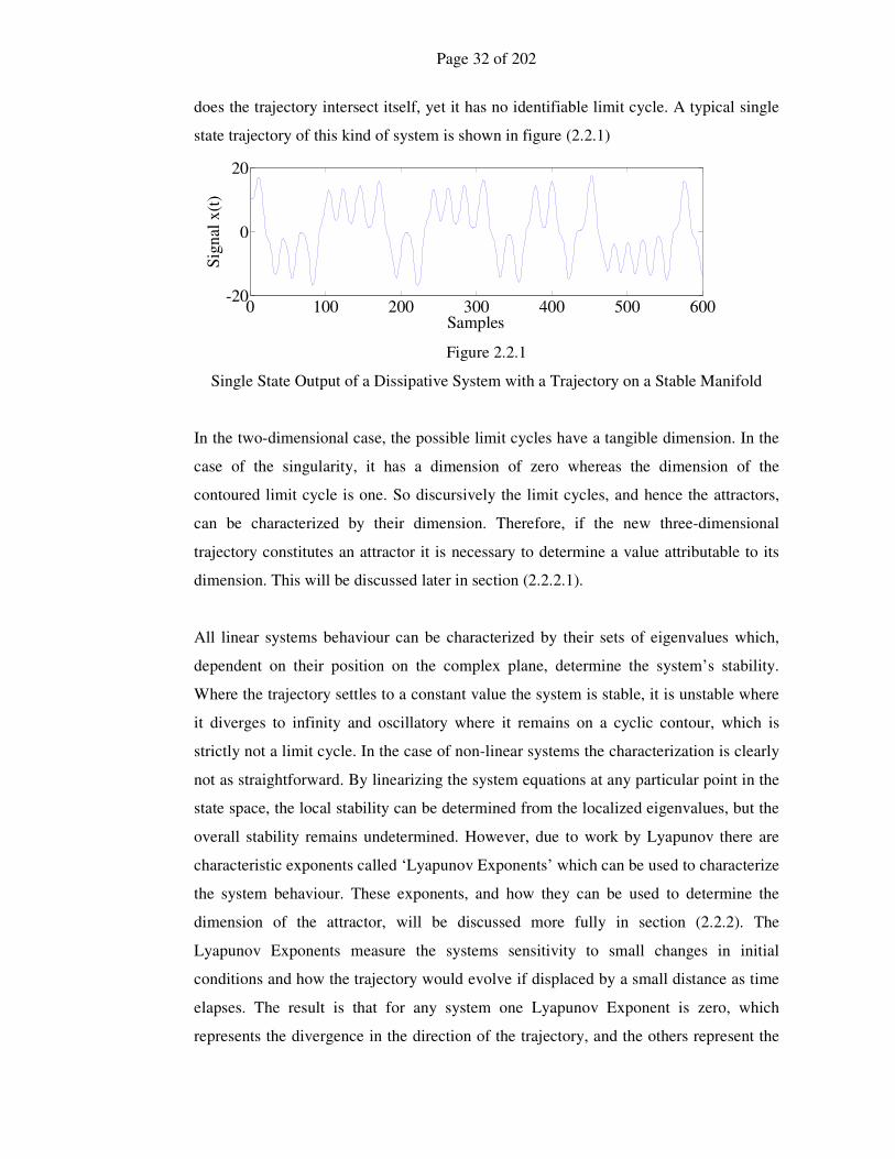
does the trajectory intersect itself, yet it has no identifiable limit cycle. A typical single
state trajectory of this kind of system is shown in figure (2.2.1)
0 100 200 300 400 500 600-20
0
20
Samples
Sig
nal
x(t
)
Figure 2.2.1
Single State Output of a Dissipative System with a Trajectory on a Stable Manifold
In the two-dimensional case, the possible limit cycles have a tangible dimension. In the
case of the singularity, it has a dimension of zero whereas the dimension of the
contoured limit cycle is one. So discursively the limit cycles, and hence the attractors,
can be characterized by their dimension. Therefore, if the new three-dimensional
trajectory constitutes an attractor it is necessary to determine a value attributable to its
dimension. This will be discussed later in section (2.2.2.1).
All linear systems behaviour can be characterized by their sets of eigenvalues which,
dependent on their position on the complex plane, determine the system’s stability.
Where the trajectory settles to a constant value the system is stable, it is unstable where
it diverges to infinity and oscillatory where it remains on a cyclic contour, which is
strictly not a limit cycle. In the case of non-linear systems the characterization is clearly
not as straightforward. By linearizing the system equations at any particular point in the
state space, the local stability can be determined from the localized eigenvalues, but the
overall stability remains undetermined. However, due to work by Lyapunov there are
characteristic exponents called ‘Lyapunov Exponents’ which can be used to characterize
the system behaviour. These exponents, and how they can be used to determine the
dimension of the attractor, will be discussed more fully in section (2.2.2). The
Lyapunov Exponents measure the systems sensitivity to small changes in initial
conditions and how the trajectory would evolve if displaced by a small distance as time
elapses. The result is that for any system one Lyapunov Exponent is zero, which
represents the divergence in the direction of the trajectory, and the others represent the
Page 33 of 202
tendency of the evolution in orthogonal directions to it. If a system has at least one
Lyapunov Exponent greater than zero, but less in magnitude than any other negative
exponent, then the systems trajectory will settle onto a stable manifold which constitutes
an attractor. The dimension of the trajectory’s flow can be determined from a
combination the Lyapunov Exponents, and if this is not an integer value the attractor is
said to be ‘strange’, and the motion is termed chaotic.
In this thesis the system used is a modified form of one due to Lorenz [45]. The system
and its properties are outlined in section (2.2.3).
2.2.1 Divergence Theorem
The statement of the Divergence Theorem is given as result (2.2.1.1) over a closed
surface S containing a volume at time t of V(t). The rate of change of volume with
respect to time is equal to the integral of the divergence of the system vector function,
with respect to the volume, bounded by a closed surface S.
Result 2.2.1.1
______________________________________________________________________
∫ ⋅∇=V
dVdt
dV)(xf (2.2.1.1)
______________________________________________________________________
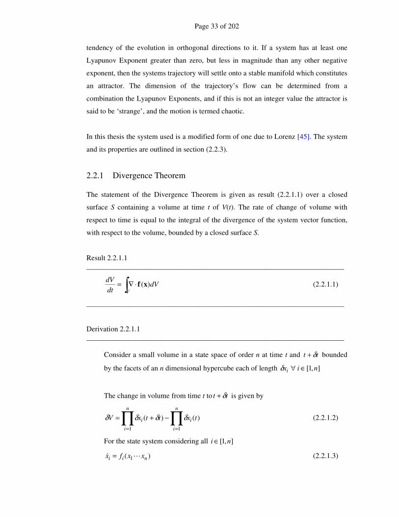
Derivation 2.2.1.1
______________________________________________________________________
Consider a small volume in a state space of order n at time t and tt δ+ bounded
by the facets of an n dimensional hypercube each of length ],1[ nixi ∈∀δ
The change in volume from time t to tt δ+ is given by
)()(
11
txttxV
n
i
i
n
i
i ∏∏==
−+= δδδδ (2.2.1.2)
For the state system considering all ],1[ ni ∈
)( 1 nii xxfx L& = (2.2.1.3)

Page 34 of 202
)(txiδ
)(1 txi+δ
)( ttxi δδ +
)(1 ttxi δδ ++
)(tx
)( tt δ+x
)(tV
)( ttV δ+
Figure 2.2.1.1
Time Evolution of a Small Regional Bounded Volume of the State Space
And each state evolves as
ttxtxttx iii δδ )()()( &+=+ (2.2.1.4)
This can be written as
txxftxttx niii δδ )()()( 1L+=+ (2.2.1.5)
So the change in the length of sides of the hypercube can be expressed as
( ) ( )txxftxtxxxxftxtxttx niiniiiiii δδδδδδ )()()()()()( 11 LLL +−+++=+
[ ] )()()( 11 txtxxfxxxxf ininiii δδδ +−+= LLL (2.2.1.6)
In the limit this gives
)(1)( txtx
fttx i
i
ii δδδδ
+
∂
∂=+ (2.2.1.7)
So the change in volume becomes
)()(1
11
txtxtx
fV
n
i
i
n
i
ii
i ∏∏==
−
+
∂
∂= δδδδ (2.2.1.8)
And this, for the small volume under consideration, reduces to
)(
11
txtx
fV
n
i
i
n
ii
i ∏∑==
⋅∂
∂= δδδ (2.2.1.9)

Page 35 of 202
This implies the following statement of the divergence theorem over the complete
volume bounded by the closed surface S
∫ ∫ ⋅∇= nn dxdxxxdt
dVLLL 11 )(f
∫ ⋅∇=V
dV)(xf (2.2.1.10)
where ∇ is the nabla vector operator on a vector function )(xf and
∑=
∂
∂=⋅∇
n
ii
ni
x
xxf
1
1 )()(
Lxf (2.2.1.11)
______________________________________________________________________
If a system is dissipative, in the sense that the volume diminishes to zero over time, it
does not imply that the system is stable; for example consider a linear system where
Axxf =)( (2.2.1.12)
Then
∑=
==⋅∇
n
i
iTr
1
)()( λAxf (2.2.1.13)
where iλ are the eigenvalues of the matrix A then equation (2.1.2.10) becomes
VTrdt
dV)(A= (2.2.1.14)
So the trace of the matrix A can be negative, and hence the volume approaches zero as
time approaches infinity, but one or more of the eigenvalues could be positive implying
that the system is unstable. Discursively, this can be interpreted as the order of the
unstable eigenvalues must be less that the order of the system; and therefore the sub
volume spanned by the trajectories of the unstable eigenvalues occupies zero volume in
the whole state space.
Page 36 of 202
)0(x∆
)0(1x
)0(2x )(tx∆
)(2 tx
)(1 tx
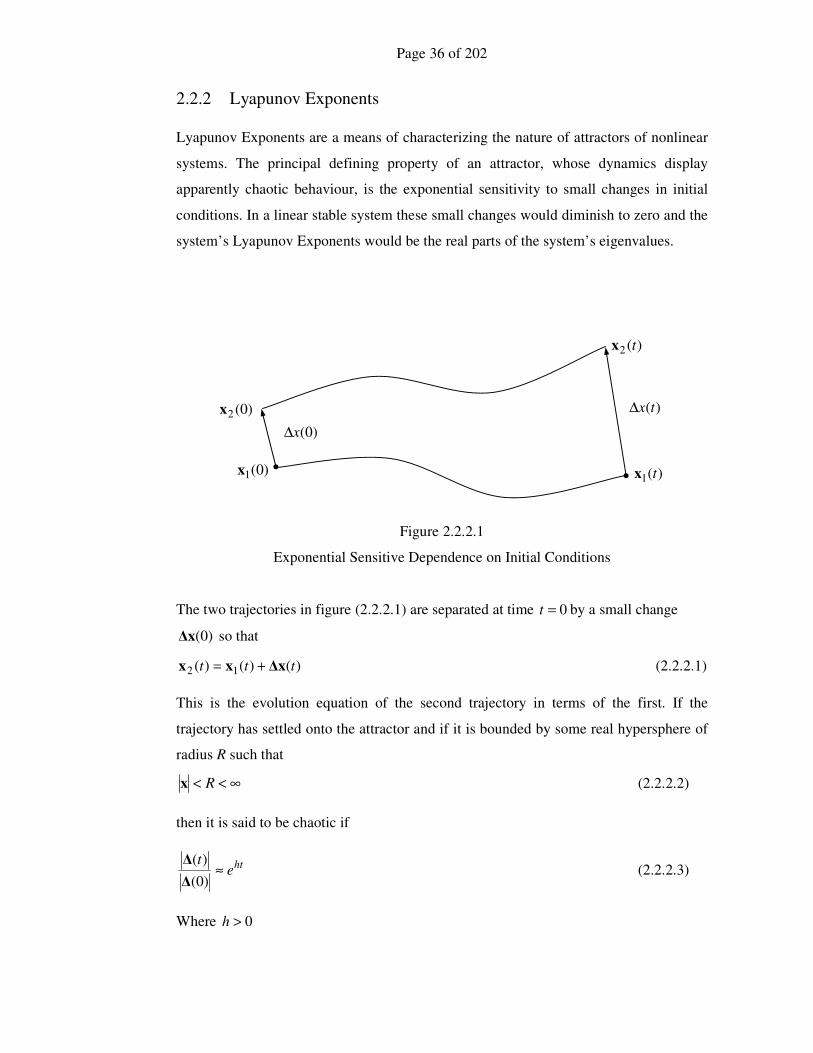
2.2.2 Lyapunov Exponents
Lyapunov Exponents are a means of characterizing the nature of attractors of nonlinear
systems. The principal defining property of an attractor, whose dynamics display
apparently chaotic behaviour, is the exponential sensitivity to small changes in initial
conditions. In a linear stable system these small changes would diminish to zero and the
system’s Lyapunov Exponents would be the real parts of the system’s eigenvalues.
Figure 2.2.2.1
Exponential Sensitive Dependence on Initial Conditions
The two trajectories in figure (2.2.2.1) are separated at time 0=t by a small change
)0(∆x so that
)()()( 12 ttt ∆xxx += (2.2.2.1)
This is the evolution equation of the second trajectory in terms of the first. If the
trajectory has settled onto the attractor and if it is bounded by some real hypersphere of
radius R such that
∞<< Rx (2.2.2.2)
then it is said to be chaotic if
hte
t≈
)0(
)(
∆
∆ (2.2.2.3)
Where 0>h
Page 37 of 202
Clearly this does not contain the whole truth, as the trajectory is not unstable with a
single positive Lyapunov Exponent value h, as equation (2.2.2.3) would imply. The
dimension of the state space could be characterized by as many Lyapunov Exponents as
there are dimensions, in much the same way as a linear system has as many eigenvalues,
each of which contribute to the overall behaviour of the system. Consideration needs to
be made as to how the trajectories move apart in directions which are orthogonal to each
other and, as the eigenvalues of a single point in a nonlinear system do not remain
constant, the Lyapunov Exponents must be an aggregated measure of the behaviour
over the whole of the attractor. In addition equation (2.2.2.3) implies that the delta
difference between two trajectories, which are arbitrarily displaced by some small
increment, needs to be considered. This can be simplified by considering some arbitrary
infinitesimal displacement from the unperturbed trajectory. If the infinitesimal
displacement is considered in the direction of the tangent vector, then the evolution of
this vector, will determine the evolution of infinitesimal displacement from the
trajectory.
The supposed exponential growth is an imposed structure on how the actual growth may
or may not take place. Consequently, it is necessary to consider some form of
averaging, to ensure that a true measure of the attractor can truly be determined.
Consider the imposed structure of equation (2.2.2.3) rearranged to give
)0()( ∆∆ht
et α= (2.2.2.4)
The dominant Lyapunov Exponent can be calculated from this equation as
)0(
)(ln
1
∆
∆ t
th ≈ (2.2.2.5)
but the terms in this equation can become exponentially large, over even a short period,
and the nature of h can be quite severely distorted, simple by the fact that the attractor is
nonlinear. It is better to consider a time averaging process, which includes an iterative
realignment and normalization of the growth. Consider the development of equation
(2.2.2.4) after a small time increment tδ
)0()( )(∆∆
tthett
δαδ +=+
)0(∆thhtee
δα=
)(teth∆
δ= (2.2.2.6)
Page 38 of 202
then the approximate Lyapunov exponent at time t, for an increase in time tδ , is given
by
)(
)(ln
1
t
tt
th
∆
∆ δ
δ
+≈ (2.2.2.6)
if the )(t∆ is reset to unity at each iteration, over a time period in which the trajectory
visits a large measure of the state space occupied by the attractor, then an
approximation for the dominant Lyapunov Exponent is given by
∑=
+≈
n
i
tittn
h
1
)(ln1
δδ
∆ (2.2.2.7)
The )( tt δ+∆ can be determined from the Jacobian variational equation of the system as
an approximation to the continuous system as
)()()(
))(()( ttt
t
ttt ∆∆
x
xf∆ +
∂
∂=+ δδ & (2.2.2.8)
where 1)( =t∆ at each iteration and tδ is sufficiently small. This integration process
can more accurately and easily be undertaken in Matlab by using various solvers of
ordinary differential equations. Given that a satisfactory integration algorithm is used
then the updated vector can be found. However, for a state space system of dimension q
there are q Lyapunov Exponents. In order to separate out each of these exponents,
without resorting to too complex methods, consider how an orthonormal set of basis
vectors, based on the tangent vector, is transformed by the Jacobian variational equation
over the time period tδ ; this is tantamount to considering how the tangent vector to the
trajectory varies given an arbitrary starting point. Then if this distorted set of basis
vectors has the growth in each direction determined, and it is re-orthonormalized at each
iteration, then the effects of the non-linearities of the attractor can be ameliorated and
the individual Lyapunov Exponents calculated. The re-orthonormalization of the
distorted set of basis vectors is achieved using the Gram-Schmidt process, which also
determines the orthogonal increase in the vector components of the resultant set. A
Matlab algorithm for achieving this is listed in appendix (A). Methods are alluded to in
[46], but the above developed method has proved to be very robust and reliable on all
the chaotic systems it has been tested on.
Page 39 of 202
2.2.3 Fractal Dimensions
The whole concept of dimension and measure is not within the scope of this thesis;
neither for the purposes of the research is it necessary to fully understand it, however
some information will prove useful for firstly illustrating the fractal nature of chaotic
attractors, from an elegant conjecture proposed by Kaplan and Yorke [47], and secondly
for choosing alternative systems in any further research.
An attractor is an infinite collection of points in some dimensional space and one of its
basic properties is its dimension. If a simple stable linear system is considered then its
attractor is a singular point, which is the steady state of the trajectory in the state space,
and clearly this has a dimension of zero. Similarly, a non-linear two dimensional system
with a limit cycle settles to a curve in the state space and has an understandable
dimension of one. However, chaotic attractors do not have such obvious dimensions,
and one of the properties of a chaotic or strange attractor, is that it has a fractional
dimension termed a fractal dimension.
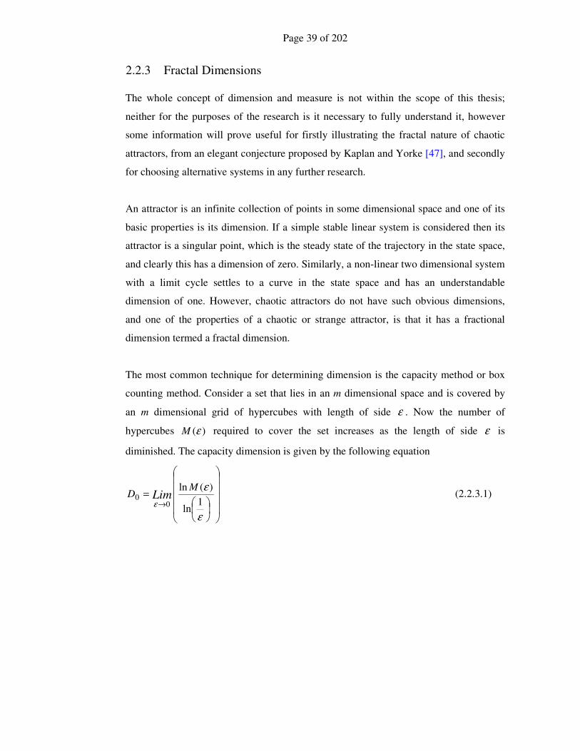
The most common technique for determining dimension is the capacity method or box
counting method. Consider a set that lies in an m dimensional space and is covered by
an m dimensional grid of hypercubes with length of side ε . Now the number of
hypercubes )(εM required to cover the set increases as the length of side ε is
diminished. The capacity dimension is given by the following equation
=
→
ε
ε
ε 1ln
)(ln
00
MD Lim (2.2.3.1)
Page 40 of 202
(a)
ε
(b)
ε
(c)
ε
Figure 2.2.3.1
Capacity Dimension Box Counting
(a) Singular Point Set, (b) Curve Set and (c) Regional Set
Consider the three examples given in figure (2.2.3.1) for a dimension of 2=m .
For case (a) 1)( =εM and therefore
00 =D as 0→ε .
For case (b) ε
εL
M ∝)( where L is the length of the curve, therefore
10 =D as 0→ε .
And finally
For case (c) 2
)(ε
εA
M ∝ where A is the area of the region, therefore
20 =D as 0→ε .
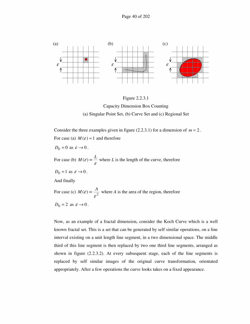
Now, as an example of a fractal dimension, consider the Koch Curve which is a well
known fractal set. This is a set that can be generated by self similar operations, on a line
interval existing on a unit length line segment, in a two dimensional space. The middle
third of this line segment is then replaced by two one third line segments, arranged as
shown in figure (2.2.3.2). At every subsequent stage, each of the line segments is
replaced by self similar images of the original curve transformation, orientated
appropriately. After a few operations the curve looks takes on a fixed appearance.
Page 41 of 202
Figure 2.2.3.2
First Four Stages of the Koch Curve
Clearly the line length tends towards infinity since at each operation it increases by 3
4of
the original length, but the area is clearly confined and is less than unity. In fact it can
be trivially shown to tend towards20
3.
So to calculate the capacity dimension choose an appropriate ε .
Let
n
=
3
1ε (2.2.3.2)
where n is the transformation iteration. Because the result is a line then ε
εL
M ∝)( so
n
n
n
KKM 4
3
1
3
4
)( ⋅=
=ε (2.2.3.3)
Page 42 of 202
where K is an arbitrary constant.
Finally the capacity dimension is given by
26186.13ln
4ln
3ln
4lnln
3ln
4ln0 ==
+=
⋅=
∞→∞→ n
nKKD LimLim
nn
n
n
(2.2.3.4)
This dimensional measure is useful for static sets but it does not account for a
dynamical system, because the trajectory of the chaotic attractor in the state space can
spend considerably longer in some regions than in others. Therefore, if a simple
capacity method is used, as with the 0D dimension, then an unrepresentative measure is
obtained. A measure known as the information dimension has been defined and is
referred to in [46] and is given by
=
∑=
→ ε
µµ
ε
ε ln
ln
)(
1
01
i
M
i
i
LimD (2.2.3.5)
where the iµ are the natural measures for each hypercube iC . This is defined by the
amount of time spent by the trajectory in that hypercube divided by the total time, as
this time tends towards infinity, that is
( )
=
∞→ T
TCi
Ti Lim
),0(, xηµ (2.2.3.6)
where ( )TCi ),0(,xη is the time measure of a hypercube iC with an initial state )0(x at
time T.
This is clearly a very difficult dimension to evaluate, but a conjecture made by [46]
states that the information dimension is the same as a measure of dimension known as
the Lyapunov dimension for typical attractors, and is defined as
∑=
+
+=
K
i
iK
L hh
KD
11
1 (2.2.3.7)
where the Lyapunov Exponents ih are arranged in ascending order and K is the largest
integer given by the number of Lyapunov Exponents greater than or equal to zero.

Page 43 of 202
That is
( ) ( )( )∑=
−−=
m
i
ii hhmK
1
2 sgnsgn2
1 where
>
=
<−
=
0:1
0:0
0:1
)sgn(
x
x
x
x (2.2.3.8)
for the Lorenz system described in section (2.2.4) the Lyapunov Exponents are given as
504.14,0.0,832.0 321 −=== hhh hence 2=K and 0574.223
1 =+=h
hDL .
This result is supported by inspection of figures (2.2.4.1) and (2.2.4.2), which show
curved surface like behaviours in two distinct regions, suggesting a potentially slightly
higher dimension than two.
2.2.4 Lorenz System
The Lorenz system of equations is well known [45]. The nonlinear state equations are
given as the dynamical vector state equation
))(()( tt xfx =& (2.2.4.1)
and explicitly as
)()()( 211 txtxtx σσ +−= (2.2.4.2)
)()()()()( 31212 txtxtxtrxtx −−= (2.2.4.3)
)()()()( 3213 txtxtxtx β−= (2.1.4.4)
If the parameters are set to 10=σ , 28=r and 3/8=β then the system is dissipative,
has one Lyapunov Exponent greater than zero and is therefore chaotic. This is
demonstrated as follows.
Consider the linearized system by the first order expansion of equation (2.2.4.1) as
))(()( tttt δδ +=+ xfx& (2.2.4.5)
tdt
td
t
ttt
dt
tdt δδ
)(
)(
))(())((
)()(
x
x
xfxf
xx
∂
∂+=+
&& (2.2.4.6)
The variational Jacobian is given by
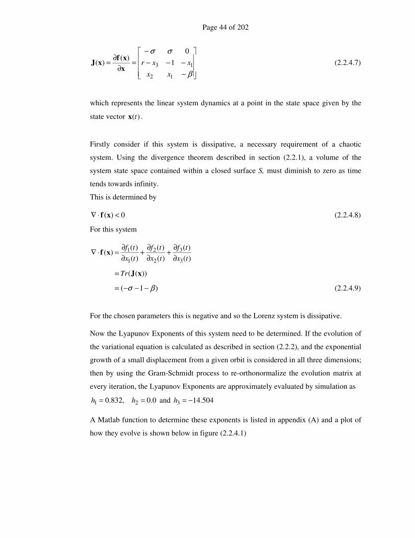
Page 44 of 202
−
−−−
−
=∂
∂=
β
σσ
12
13 1
0)(
)(
xx
xxrx
xfxJ (2.2.4.7)
which represents the linear system dynamics at a point in the state space given by the
state vector )(tx .
Firstly consider if this system is dissipative, a necessary requirement of a chaotic
system. Using the divergence theorem described in section (2.2.1), a volume of the
system state space contained within a closed surface S, must diminish to zero as time
tends towards infinity.
This is determined by
0)( <⋅∇ xf (2.2.4.8)
For this system
)(
)(
)(
)(
)(
)()(
3
3
2
2
1
1
tx
tf
tx
tf
tx
tf
∂
∂+
∂
∂+
∂
∂=⋅∇ xf
))(( xJTr=
)1( βσ −−−= (2.2.4.9)
For the chosen parameters this is negative and so the Lorenz system is dissipative.
Now the Lyapunov Exponents of this system need to be determined. If the evolution of
the variational equation is calculated as described in section (2.2.2), and the exponential
growth of a small displacement from a given orbit is considered in all three dimensions;
then by using the Gram-Schmidt process to re-orthonormalize the evolution matrix at
every iteration, the Lyapunov Exponents are approximately evaluated by simulation as
0.0,832.0 21 == hh and 504.143 −=h
A Matlab function to determine these exponents is listed in appendix (A) and a plot of
how they evolve is shown below in figure (2.2.4.1)

Page 45 of 202
0 2 4 6 8 10-30
-20
-10
0
10
20
Ly
apu
no
v E
xp
on
ents
Time
h1
h2
h3
Figure 2.2.4.1
Lyapunov Exponent Evolution Plots
The results show one exponent less than zero, which discursively means that in this
dimension the tendency to move away from the trajectory diminishes to zero; one is
equal to zero which is the exponent in the direction of the trajectory and as the state
progresses along this path, the tendency to diverge from it must be zero; and finally one
is greater than zero which implies a chaotic system which, due the other non zero
exponent being negative, suggests that the bounded trajectories lie on smooth curved
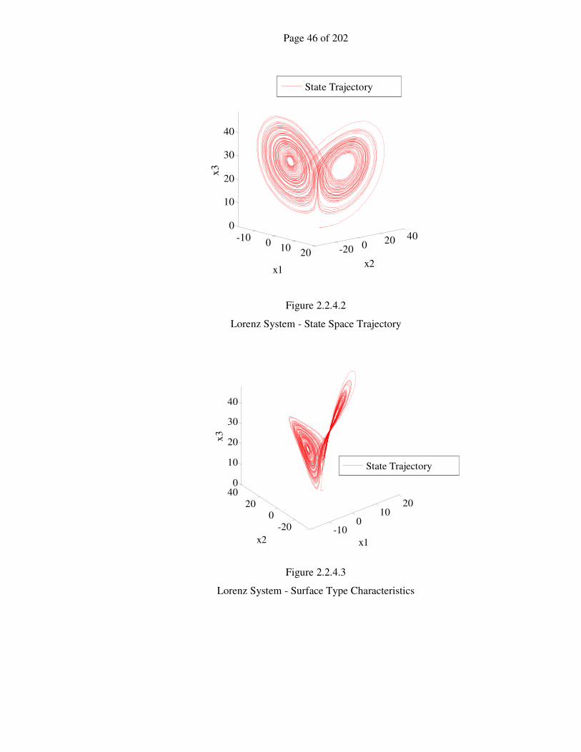
surfaces within the three dimensional state space. This is demonstrated in figures
(2.2.4.2) and (2.2.4.3) which show a time progression of the system, with the suggested
parameters, and the surface type characteristic.
The Lorenz system described is therefore a good candidate for testing the new
communication schemes described in chapter 3.
Page 46 of 202
-100
1020 -20 0 20 40
0
10
20
30
40
x2x1
x3
State Trajectory
Figure 2.2.4.2
Lorenz System - State Space Trajectory
-100
1020
-20
020
400
10
20
30
40
x1x2
x3
State Trajectory
Figure 2.2.4.3
Lorenz System - Surface Type Characteristics
Page 47 of 202
2.2.5 Alternative Systems
The Lorenz system is an example of a chaotic system displaying one degree of chaos;
that is, that it has one Lyapunov Exponent greater than zero and thus the chaos has a
‘planar’ or surface type of habitual behaviour. This surface type of behaviour, in any set
of dimensions of a state space system, generated by the system having a Lyapunov
dimension of close to two, manifests itself in a periodic like manner. This is clearly
illustrated by figure (2.2.1) and it is easily appreciated that this type of periodicity can
be easily detected. For this reason, degree one chaotic systems are not the best choice
for chaotic secure communication schemes. This periodicity can add further
complications for the proposed scheme architecture, which is the main subject of this
thesis. Further reference will be made to this in chapter 3. Systems which do not so
readily display periodic type behaviour, usually have a degree of chaos of greater than
one, and are termed hyperchaotic. Systems that are not truly hyperchaotic, but display
hyperchaotic behaviour and good clarity for the understanding of the communications
schemes, usually contain non-linearities which are constructed from discontinuities [7]
and this is not beneficial to a secure communications structure. All continuous three
dimensional systems, which do not contain discontinuities, are of degree one.
2.3 Synchronization Methods
The concept of using synchronization methods in communications schemes is based on
the idea that two similar circuits or state space systems, one in the transmitter and the
other in the receiver, can have at any particular time, the same dynamical state. The
means by which this can be achieved has been the subject of a great deal of research.
There are three basic methods of synchronization available. The first is some form of
external reference such as an absolute time from a GPS satellite or other reliable source.
If the circuit or dynamical system can use this to determine its current state, then
synchronization between disparate systems can be achieved. The second would rely on
the manufacture of highly accurate components and internal clocks, which would ensure
that the error between the two systems would not vary by a given margin, in the time
between some form of system coordinating calibration. The final method to achieve
synchronization is by communicating, in some way, the state of the transmitter over the
transmission channel to the receiver. The problem then becomes one of rejecting the
Page 48 of 202
noise on the transmission channel, separating out the message contained in the signal
and ensuring that the signal synchronizes the circuit or state of the dynamical system.
The final problem is the one reviewed in this chapter.
2.3.1 Drive Response Synchronization
The work that is normally seen as the initial work on drive response systems is by
Pecora and Carroll [4]. They introduce the concept of synchronizing two systems, a
response system, using an observed driving signal, and a corresponding driving system
producing it. The systems can be seen as receiver and transmitter in a communication
scheme. The two systems are the same, and the requirement is to ensure that the state of
the response system follows the state of the driving system, after some small
synchronizing time despite, the initial conditions. Pecora and Carroll showed that the
two systems would indeed synchronize, if the system could be split into two stable
subsystems, with the driven subsystem having negative definite conditional Lyapunov
Exponents. This implies that the state trajectory error would tend towards zero as time
tends towards infinity. In a further paper [5], they discuss extending the linear stability
theorem to chaotic systems, and show that the convergence of states is related to the
conditional Lyapunov Exponents and the eigenvectors of the Principal Matrix Solution
of the chosen subsystem. To illustrate how this method works, consider the chaotic
system due to Lorenz [45] as the drive system and how it is split into subsystems for the
purpose of synchronization. In turn it will be demonstrated how this method and the
synchronization property can be used as a communication scheme.
Consider the Lorenz system equations as the drive system
)(ufu =&
[ ]zyxT =u
−
−−
+−
=
zxy
xzyrx
yx
β
σσ
)(uf (2.3.1.1)
where u is the state vector and )(uf is the system equation set.
Now partition the system into two subsystems with a singular state variable v , a partial
state vector w and their associated subsystem equations.
Page 49 of 202
The system equations are
),( wvgv =&
),( whw v=& (2.3.1.2)
where the separated states are xv = and [ ]zyT =w .
The set of equations (2.3.1.2) can be considered as the drive system, and the single state
variable will be considered as the observed signal that will be used to synchronize the
two systems. Now consider the driven or response set of subsystems where the response
system state variables are superscripted as w′
),( whw ′=′ v&
),( w′′=′ vgv& (2.3.1.3)
Where explicitly these can be written as
′−′
′−′−=′
21
21),(
wwv
wvwrvv
βwh
1),( wvvg ′+′−=′′ σσw (2.3.1.4)
Now look at the variational equation of the first subsystem in equation (2.3.1.3)
ww∆w −′=
∆ww
hw∆
∂
∂=& (2.3.1.5)
And w
h
∂
∂is given by
−−=
∂
∂
βv
v1
w
h (2.3.1.6)
The Lyapunov Exponents of equation (2.3.1.5) are termed as conditional Lyapunov
Exponents and if they are negative definite, then this is a necessary but not sufficient
condition for synchronisation. It does not account for the set of all possible initial
conditions and is not defined for initial conditions at infinity. If, however, the system’s
Page 50 of 202
trajectory has settled onto the attractor then this condition is sufficient to ensure
synchronization.
For the Lorenz system with parameters set to
10=σ , 28=r , 3/8=β
The conditional Lyapunov Exponents, calculated using the method described in section
(2.2.2), are
81.11 −=h and 86.12 −=h
This implies that the response subsystem is not chaotic; the response systems partial
state vector will synchronize asymptotically to the drive system’s partial state vector
and consequently the final remaining state can be reconstructed using equation (2.3.1.3).
This results in a fully synchronized state vector in the response system. It should be
noted that the variational equation of the smaller subsystem, is actually a linear system
with an eigenvalue of σ− , which means that the subsystem is asymptotically stable and
ensures synchronization. Clearly the choice of subsystems is not a simple one and the
conditional Lyapunov Exponents of some of the possible systems may be unstable. The
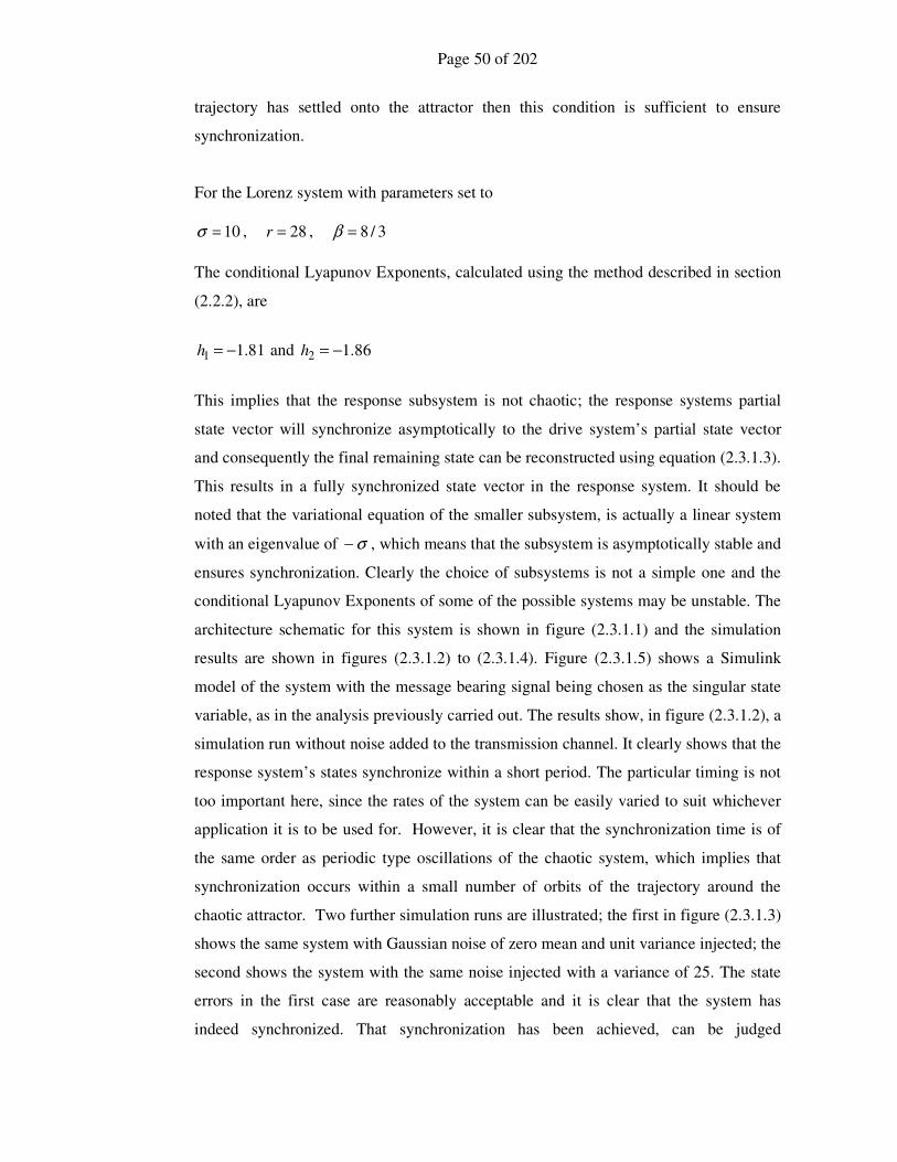
architecture schematic for this system is shown in figure (2.3.1.1) and the simulation
results are shown in figures (2.3.1.2) to (2.3.1.4). Figure (2.3.1.5) shows a Simulink
model of the system with the message bearing signal being chosen as the singular state
variable, as in the analysis previously carried out. The results show, in figure (2.3.1.2), a
simulation run without noise added to the transmission channel. It clearly shows that the
response system’s states synchronize within a short period. The particular timing is not
too important here, since the rates of the system can be easily varied to suit whichever
application it is to be used for. However, it is clear that the synchronization time is of
the same order as periodic type oscillations of the chaotic system, which implies that
synchronization occurs within a small number of orbits of the trajectory around the
chaotic attractor. Two further simulation runs are illustrated; the first in figure (2.3.1.3)
shows the same system with Gaussian noise of zero mean and unit variance injected; the
second shows the system with the same noise injected with a variance of 25. The state
errors in the first case are reasonably acceptable and it is clear that the system has
indeed synchronized. That synchronization has been achieved, can be judged
Page 51 of 202
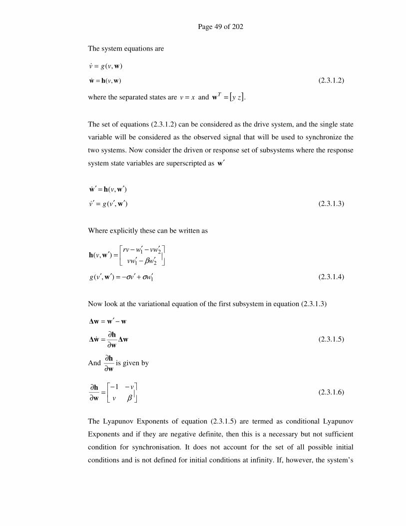
(a) )(uf
s
3I
u u& v Tc
(b)
),( wvg v&
),( wh v w&
v
w
s
1
s
2I
(c)
),( w′′vg v′&
),( wh ′v w′&
v′
w′
s
1
s
2I
v
qualitatively by the fact that the response system states do follow the drive system’s
states over the simulation period. However, in the second case the state errors are
similar, throughout the simulation, to the initial errors and it is quite unclear that
synchronization has been achieved. Again from a qualitative point of view the response
system’s states do not follow the drive system’s states. However this approximate
synchronization may be acceptable dependent on the application.
Figure 2.3.1.1
Drive Response System
(a) Full State Vector Drive System, (b) Single State Variable and Partial State
Vector Drive System and (c) Single State Variable And Partial State Vector
Estimator in the Response System
Page 52 of 202
0 1 2 3 4 5-50
-25
0
25
50(a)
Time (secs)
Sta
te
0 1 2 3 4 5-50
-25
0
25
50(b)
Time (secs)
Sta
te E
stim
ate
0 1 2 3 4 5-20
-10
0
10
20(c)
Time (secs)
Sta
te E
rro
r
0 1 2 3 4 5-5
0
5(d)
Time (secs)
Sta
te N
ois
e
Figure 2.3.1.2
Simulation Results without Noise
(a) Drive System States
(b) Response System States
(c) State Errors
(d) State additive noise

Page 53 of 202
0 1 2 3 4 5-50
-25
0
25
50(a)
Time (secs)
Sta
te
0 1 2 3 4 5-50
-25
0
25
50(b)
Time (secs)
Sta
te E
stim
ate
0 1 2 3 4 5-20
-10
0
10
20(c)
Time (secs)
Sta
te E
rro
r
0 1 2 3 4 5-5
0
5(d)
Time (secs)
Sta
te N
ois
e
Figure 2.3.1.3
Simulation Results with Gaussian Noise
Mean 0=µ , Variance 12 =σ
(a) Drive System States
(b) Response System States
(c) State Errors
(d) State additive noise

Page 54 of 202
0 1 2 3 4 5-50
-25
0
25
50(a)
Time (secs)
Sta
te
0 1 2 3 4 5-50
-25
0
25
50(b)
Time (secs)
Sta
te E
stim
ate
0 1 2 3 4 5-20
-10
0
10
20(c)
Time (secs)
Sta
te E
rror
0 1 2 3 4 5-15
-10
-5
0
5
10
15(d)
Time (secs)
Sta
te N
ois
e
Figure 2.3.1.4
Simulation Results with Gaussian Noise
Mean 0=µ , Variance 252 =σ
(a) Drive System States
(b) Response System States
(c) State Errors
(d) State additive noise

Page 55 of 202
Figure 2.3.1.5
Simulink Model of Synchronization System
Page 56 of 202
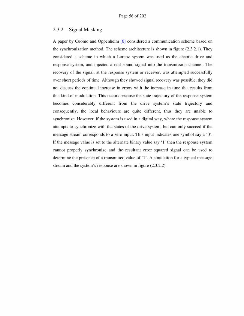
2.3.2 Signal Masking
A paper by Cuomo and Oppenheim [6] considered a communication scheme based on
the synchronization method. The scheme architecture is shown in figure (2.3.2.1). They
considered a scheme in which a Lorenz system was used as the chaotic drive and
response system, and injected a real sound signal into the transmission channel. The
recovery of the signal, at the response system or receiver, was attempted successfully
over short periods of time. Although they showed signal recovery was possible, they did
not discuss the continual increase in errors with the increase in time that results from
this kind of modulation. This occurs because the state trajectory of the response system
becomes considerably different from the drive system’s state trajectory and
consequently, the local behaviours are quite different, thus they are unable to
synchronize. However, if the system is used in a digital way, where the response system
attempts to synchronize with the states of the drive system, but can only succeed if the
message stream corresponds to a zero input. This input indicates one symbol say a ‘0’.
If the message value is set to the alternate binary value say ‘1’ then the response system
cannot properly synchronize and the resultant error squared signal can be used to
determine the presence of a transmitted value of ‘1’. A simulation for a typical message
stream and the system’s response are shown in figure (2.3.2.2).
Page 57 of 202
(a) )(uf
s
3I
u u& v Tc
(c)
),( w′′vg v′&
),( wh ′v w′&
v′
w′
s
1
s
2I
sv +
(b)
Message
τMratesymbol
s m
Figure 2.3.2.1
Signal Masking System Architecture
(a) Full State Vector Drive System, (b) Message Sampling,
(c) Single State Variable and Partial State Vector Estimator in the Response System

Page 58 of 202
0 20 40 60 80 100-1
0
1
2(a)
Time (secs)
Mes
sag
e
0 20 40 60 80 100-20
-10
0
10
20
Time (secs)
Sig
nal
(b)
0 20 40 60 80 100-15
-10
-5
0
5
10
15(c)
Time (secs)
Sig
nal
Err
or
0 20 40 60 80 100-20
-10
0
10
20(d)
Time (secs)
Sig
nal
Est
imat
e
0 20 40 60 80 1000
20
40
60
80
100
120
140(e)
Time (secs)
Sq
uar
ed E
rro
r
Figure 2.3.2.2
Signal Masking Messages Simulation
(a) Additive Message
(b) Transmitted Signal
(c) Error Between Signal and Signal Estimate
(d) Signal Estimate
(e) Signal Error Squared

Page 59 of 202
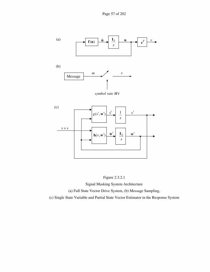
2.3.3 Parameter Variation
In this method, the system itself is designed to be used in a digital way, which alleviates
the real modulation problems of the masking method. The system architecture is shown
in figure (2.3.3.1). The message consists of two symbols representing ‘1’s and ‘0’s
which are represented in the drive system by one of the nonlinear parameters in the
system equations. For a symbol ‘0’ the value of the parameter is set to one value and for
the symbol ‘1’ it is set to another. Again the response system attempts to synchronize to
the state trajectory of the drive system, but can only succeed if the drive system’s
parameter is the same as its own corresponding value. This indicates the first symbol
value has been transmitted and the response system will synchronize. If the message
value is set to the alternate binary value, then the response system cannot properly
synchronize, and the resultant squared error signal can be used to determine the
presence of the other transmitted value. A simulation for a typical message stream and
the system’s response are shown in figure (2.3.3.2).
Page 60 of 202
)(2,1 ufs
3I
u u& v Tc
Message s m
τMratesymbol
),( w′′vg v′&
),( wh ′v w′&
v′
w′
s
1
s
2I
v
(a)
(b)
Figure 2.3.3.1
Parameter Variation System
(a) Full State Vector Drive System with Parameter varied by Message
(b) Single State Variable and Partial State Vector Estimates in the Response System

Page 61 of 202
0 20 40 60 80 100-1
0
1
2(a)
Time (secs)
Mes
sag
e
0 20 40 60 80 100-20
-10
0
10
20
Time (secs)
Sig
nal
(b)
0 20 40 60 80 100-5
0
5(c)
Time (secs)
Sig
nal
Err
or
0 20 40 60 80 100-20
-10
0
10
20(d)
Time (secs)
Sig
nal
Est
imat
e
0 20 40 60 80 1000
5
10
15
20(e)
Time (secs)
Sq
uar
ed E
rro
r
Figure 2.3.3.2
Parameter Variation Messages Simulation
(a) Additive Message
(b) Transmitted Signal
(c) Error Between Signal and Signal Estimate
(d) Signal Estimate
(e) Signal Error Squared
Page 62 of 202
2.3.4 Chaotic Attractor Synchronization
The parameter variation method of section (2.3.3) can only represent two possible
symbols in the message set, because the response system can either synchronize or it
fails to. This is a simplified version of a method based on a scheme utilizing differing
chaotic attractors to represent each different symbol. Instead of having a single response
system, which can either synchronize or not, representing a two state message set, there
are as many chaotic systems as there are symbols in the message set itself. So the
scheme consists of a number of different systems, each representing a different symbol
in both the transmitter or drive system side and the receiver or response system. This
difference can be as simple as a single parameter in a system or a set of completely
different systems. The signal transmitted is the signal from the particular system that
represents the message symbol at that sample period and therefore, the only system in
the receiver that synchronizes is the one corresponding to the same message symbol. It
is important to realize that the chaotic attractor here represents the symbol [13]. Below
the system diagram figure (2.3.4.1) represents a system with only two message symbols,
and the figures (2.3.4.2-B) (e) and (h) show the squared error terms for each attractor for
the corresponding message in figure (2.3.4.1-A )(a)
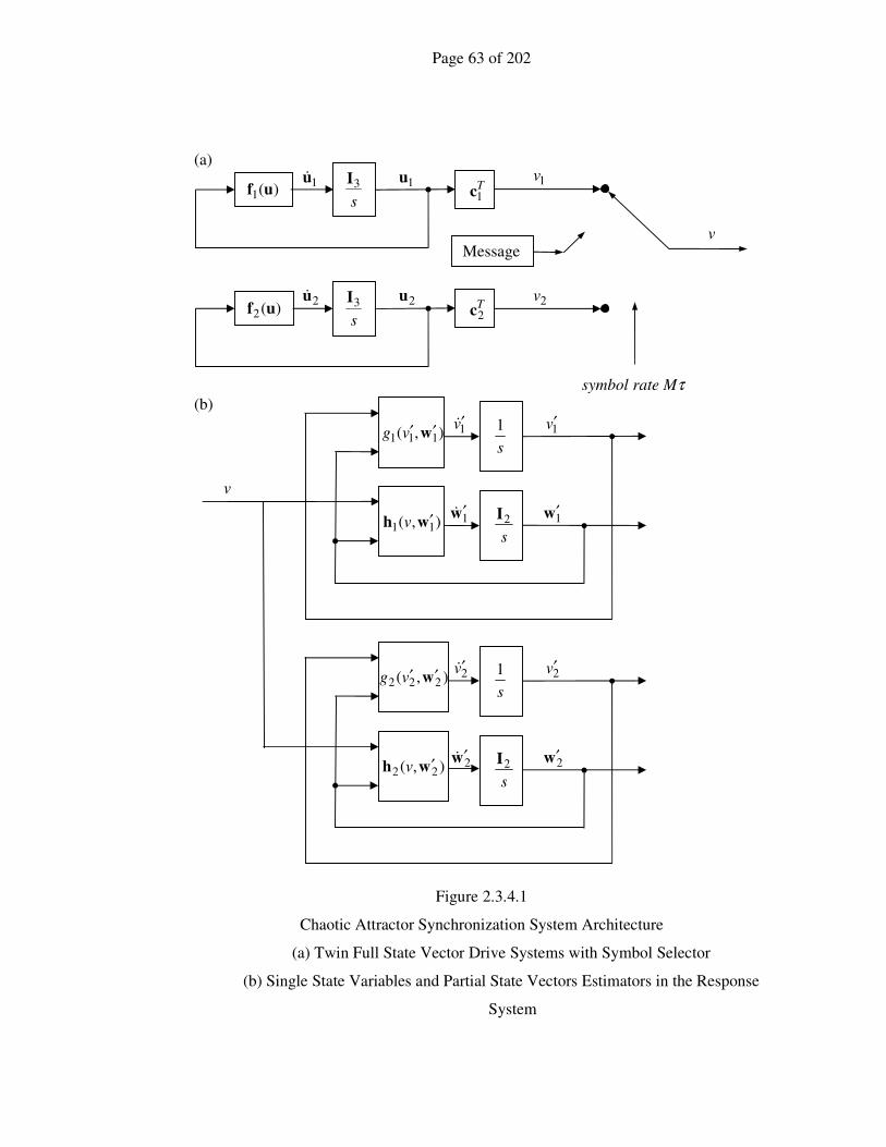
Page 63 of 202
)(1 uf s
3I 1u 1u& 1v
T1c
)(2 uf s
3I
2u 2u& 2v T2c
Message
τMratesymbol
),( 111 w′′vg 1v′&
),( 11 wh ′v 1w′&
1v′
1w′
s
1
s
2I
v
),( 222 w′′vg 2v′&
),( 22 wh ′v 2w′&
2v′
2w′
s
1
s
2I
(b)
(a)
v
Figure 2.3.4.1
Chaotic Attractor Synchronization System Architecture
(a) Twin Full State Vector Drive Systems with Symbol Selector
(b) Single State Variables and Partial State Vectors Estimators in the Response
System

Page 64 of 202
0 20 40 60 80 100-1
0
1
2
Time (secs)
Mes
sag
e
(a)
0 20 40 60 80 100-20
-10
0
10
20(b)
Time (secs)
Sig
nal
0 20 40 60 80 100-20
-10
0
10
20(c)
Time (secs)
Est
imat
e A
0 20 40 60 80 100-20
-10
0
10
20(d)
Time (secs)
Est
imat
e B
Figure 2.3.4.2-A
Chaotic Attractor Synchronization Messages Simulation
(a) Message, (b) Transmitted Signal, (c) Error Between Signal ‘A’ and Signal ‘A’
Estimate, (d) Signal ‘A’ Estimate.

Page 65 of 202
0 20 40 60 80 100-5
0
5(e)
Time (secs)
Err
or
A
0 20 40 60 80 100-5
0
5(f)
Time (secs)
Err
or
B
0 20 40 60 80 1000
5
10
15
20(g)
Time (secs)
Sq
uar
ed E
rro
r A
0 20 40 60 80 1000
5
10
15
20(h)
Time (secs)
Sq
uar
ed E
rro
r B
Figure 2.3.4.2-B
Chaotic Attractor Synchronization Messages Simulation
(e) Signal ‘A’ Error Squared, (f) Error Between Signal ‘B’ and Signal ‘B’ Estimate, (g)
Signal ‘B’ Estimate and (h) Signal ‘B’ Error Squared

Page 66 of 202
2.4 Non-Reference Correlation Methods
2.4.1 Symmetric Chaos Shift Keying
The Symmetric Chaos Shift Keying (SCSK) method employs the advantages offered by
the inherent phase synchronization given by the drive response principle and well
understood correlation methods. The carrier is generated by a single or combination of
states of a chaotic system, which is then modulated with a message symbol or bit code
1±=kb . The operation is illustrated in figure (2.4.1.1)
Figure 2.4.1.1
Symmetric Chaos Shift Keying Architecture
(a) SCSK Transmitter and (b) SCSK Receiver
This type of scheme is considered by [13]
Recovery of the transmitted signal is effectively a two-stage process. The receiver
contains a similar chaotic generator to the transmitter, which is synchronized by the
drive response principles, with the incoming modulated signal. This estimated state
signal is then correlated with the received signal to recover the transmitted bit code as
outline below. The principle of this method relies on the fact that the system is
xcT )(xfx =& X
)(ts )(txi
τMratebk
1
(a) Transmitter
X ∫=
τ
τ
M
i dttrtxM
S
0
)()(ˆ1
Decoder
)(tr
)(ˆ txi xc
T )(xfx =&
(b) Receiver

Page 67 of 202
symmetrical in one or a combination of the states chosen as the modulation signal. It is
supposed here that the conditions of the drive response principle are adhered to, that is
that the conditional Lyapunov Exponents of each of the subsystems are not chaotic.
This type of technique does require that the nonlinear system is even in the combination
of the states chosen to be used as the message bearer. This is necessary to ensure that
the driven system in the receiver synchronizes despite the sign of the encoding.
Derivation 2.4.1.1
______________________________________________________________________
For the continuous form of SCSK the modulation signal is given as
)()( tts T xc= (2.4.1.1)
And the systems equation as
)()( xfx =t& (2.4.1.2)
Consider an example modulation signal
)()( txts i=
),()( x)
& iii xftx =
),()( x)
& iii xftx −= (2.4.1.3)
)(xf is even and thus symmetric function in the single state )(txi and )(tx)
is the
remaining state vector. Now consider the correlation integral over an interval
],0[ τM where M is the number of samples in the interval
dttrtxM
S
M
i )()(ˆ1
0
∫=
τ
τ (2.4.1.4)
Here the state estimate )(ˆ txi is contaminated by Gaussian White noise as is the
received message bearing signal )(tr which is modulated with the values 1±=kb
these signals are given as
)()()(ˆ tetxtx ii +=
)()()( tntxbtr ik += (2.4.1.5)
Substituting equations (2.4.1.5) into (2.4.1.4) yields
( )( )dttntxbtetxM
S ik
M
i )()()()(1
0
++= ∫τ
τ (2.4.1.6)

Page 68 of 202
This gives
)()(1
0
2tdttxb
MS
M
ik ετ
τ
+= ∫ (2.4.1.7)
Where the noise signal is elaborated as
dttntetxtebtntxM
t
M
iki∫ ++=
τ
τε
0
)()()()()()(1
)( (2.4.1.8)
The following properties follow from the noise signals being Gaussian White:
{ } 0)( =Ε te , { } 0)( =Ε tn , { } 0)()( =Ε tnte and { } 0)()( =Ε tntz where )(tz is any
other zero mean process then
{ } 0)( =Ε tε (2.4.1.9)
And the integral becomes
xk PbS = (2.4.1.10)
Now as the power of the signal can be generated as
{ })()(1 2
0
2txPdttx
MP x
M
x Ε=⇔= ∫τ
τ (2.4.1.11)
The original signal can be recovered as
xk
P
Sb = (2.4.1.12)
______________________________________________________________________
The principal disadvantage with this approach, and the derivation of its name, is the
requirement that the chaotic process is an even or symmetric function in a single or
some combination of states. This requirement comes from the need for the receiver to
be able to synchronize with the received signal, regardless of the sign of the bit code.
This constraint can prove difficult to achieve, and most systems of this form are
implemented using digital forms, that use two-dimensional chaotic maps.
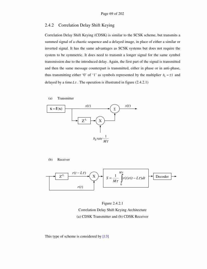
Page 69 of 202
2.4.2 Correlation Delay Shift Keying
Correlation Delay Shift Keying (CDSK) is similar to the SCSK scheme, but transmits a
summed signal of a chaotic sequence and a delayed image, in place of either a similar or
inverted signal. It has the same advantages as SCSK systems but does not require the
system to be symmetric. It does need to transmit a longer signal for the same symbol
transmission due to the introduced delay. Again, the first part of the signal is transmitted
and then the same message counterpart is transmitted, either in phase or in anti-phase,
thus transmitting either ‘0’ of ‘1’ as symbols represented by the multiplier 1±=kb and
delayed by a time τL . The operation is illustrated in figure (2.4.2.1)
Figure 2.4.2.1
Correlation Delay Shift Keying Architecture
(a) CDSK Transmitter and (b) CDSK Receiver
This type of scheme is considered by [13]
(b) Receiver
Z-L
∫ −=
τ
ττ
M
dtLtrtrM
S
0
)()(1
Decoder
)(tr
)( τLtr −X
Z-L
)(xfx =&
X
)(ts )(tx
τMratebk
1
(a) Transmitter
Σ

Page 70 of 202
Recovery of signal is achieved by correlating the current signal with itself delayed by
τL . The disadvantage of this approach is that the noise rejection is not as good as
DCSK, outlined in section (2.5.1), but it has a greater transmission rate due to not
transmitting the reference.
Derivation 2.4.2.1
______________________________________________________________________
The continuous form of CDSK
)()()( τLtxbtxts k −+= ∀ ],0[ τMt ∈ (2.4.2.1)
dttrLtrM
S
M
)()(1
0
∫ −=
τ
ττ
(2.4.2.2)
)()()( tntstr +=
)()()( τττ LtnLtsLtr −+−=− (2.4.2.3)
)()()()( tnLtxbtxtr k +−+= τ
)()2()()( ττττ LtnLtxbLtxLtr k −+−+−=− (2.4.2.4)
)()(1 2
0
tdtLtxbM
S
M
k εττ
τ
+−= ∫ (2.4.2.5)
+−+−+−= ∫τ
ττττ
ε
M
k txLtntxLtxbtxLtxM
t
0
)()()()2()()(1
)(
+−−+−− )()()()2(... 2 ττττ LtxLtnbLtxLtxb kk
dttnLtntnLtxbtnLtx k )()()()2()()(... τττ −+−+− (2.4.2.6)
{ } 0)( =Ε tn , { } 0)()( =−Ε tnLtn τ and { } 0)()( =Ε tntz where )(tz is any other zero
mean process. Additionally if τkL is sufficiently large and the signal )(tx is
sufficiently varying then { } 0:0)()( >=−Ε kkLtxtx τ . This then implies that
{ } 0)( =Ε tε (2.4.2.7)
And the integral becomes
xk PbS = (2.4.2.8)

Page 71 of 202
Now as the power of the signal can be generated as
{ })()(1 2
0
2txPdttx
MP x
M
x Ε=⇔= ∫τ
τ (2.4.2.9)
The original signal can be recovered as
xk
P
Sb = (2.4.2.10)
______________________________________________________________________
2.5 Reference Correlation Methods
Reference Correlation methods overcome the problems of synchronization methods,
delayed correlation methods or systems with special structures, by transmitting for each
symbol a single or multiple set of reference signals, followed by a set of encoded
signals carrying the message. This removes the time dependency problems, the noise
problems related to synchronization and reduces the extensive effects of noise in the
transmission channels. The following sections describe some typical methods.
2.5.1 Differential Chaos Shift Keying
This is similar to the well-understood method of Binary Phase Shift Keying (BPSK). In
BPSK the underlying message bearer is sinusoidal, and for a portion of the transmitted
signal, a reference sine wave is transmitted followed by the symbol carrying part of the
signal. To represent a ‘0’ an in phase sine wave is transmitted and its anti-phase
counterpart is transmitted to represent a ‘1’. By correlating the signals at the receiver,
the signals can be time synchronized, and decrypted quite simply.
Differential Chaos Shift Keying (DCSK) is exactly analogous to BPSK, but the
underlying message carrier is a portion of a signal generated by a chaotic system. Again
the first part of the signal is transmitted as a reference, and then its counterpart is
transmitted either in phase or in anti-phase, thus transmitting either ‘0’ of ‘1’ as symbols
represented by the multiplier 1±=kb . The operation is illustrated in figure (2.5.1.1)

Page 72 of 202
Figure 2.5.1.1
Differential Chaos Shift Keying Architecture
(a) DCSK Transmitter and (b) DCSK Receiver
This type of scheme is considered by [13-19]
Recovery of the message is achieved by correlating the current signal with itself delayed
by half of the symbol transmission period τM . This approach results in the rejection of
the noise encountered in the transmission channel and the recovery of the bit code
transmitted. The noise is considered to be Gaussian White. This is demonstrated in the
following derivation.
Z-M
∫ +=
τ
ττ
M
dtMtrtrM
S
0
)()(1
Decoder )(tr
)( τMtr +
(b) Receiver
X
Z-M
)(xfx =&
X
τM
)(ts
)(tx
τMratebk
2
1
(a) Transmitter
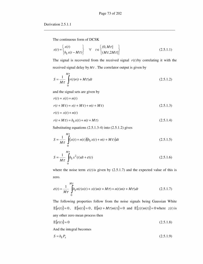
Page 73 of 202
Derivation 2.5.1.1
______________________________________________________________________
The continuous form of DCSK
−=
)(
)()(
τMtxb
txts
k
∀
∈]2,(
],0(
ττ
τ
MM
Mt (2.5.1.1)
The signal is recovered from the received signal )(tr by correlating it with the
received signal delay by τM . The correlator output is given by
dtMtrtrM
S
M
)()(1
0
ττ
τ
+= ∫ (2.5.1.2)
and the signal sets are given by
)()()( tntstr +=
)()()( τττ MtnMtsMtr +++=+ (2.5.1.3)
)()()( tntxtr +=
)()()( ττ MtntxbMtr k ++=+ (2.5.1.4)
Substituting equations (2.5.1.3-4) into (2.5.1.2) gives
( )( )dtMtntxbtntxM
S k
M
)()()()(1
0
ττ
τ
+++= ∫ (2.5.1.5)
∫ +=
τ
ετ
M
k tdttxbM
S
0
2 )()(1
(2.5.1.6)
where the noise term )(tε is given by (2.5.1.7) and the expected value of this is
zero.
dtMtntnMtntxtxtnbM
t
M
k )()()()()()(1
)(
0
τττ
ε
τ
++++= ∫ (2.5.1.7)
The following properties follow from the noise signals being Gaussian White
{ } 0)( =Ε te , { } 0)( =Ε tn , { } 0)()( =+Ε tnMtn τ and { } 0)()( =Ε tntz where )(tz is
any other zero mean process then
{ } 0)( =Ε tε (2.5.1.8)
And the integral becomes
xk PbS = (2.5.1.9)

Page 74 of 202
Now the power of the signal can be generated from the reference part of the signal
as
{ })()(1 2
0
2txPdttx
MP x
M
x Ε=⇔= ∫τ
τ (2.5.1.10)
and the original encoding can be recovered as
xk
P
Sb = (2.5.1.11)
______________________________________________________________________
This approach has good noise rejection [13][41] but is flawed by a need for the receiver
to be in phase with the transmitter. The phase locking can be quite complex, as the
message bearing signal is a spread spectrum type, which is not fixed at a particular
frequency.
2.5.2 FM Differential Chaos Shift Keying
This FM-DCSK scheme [19] extends the ideas of DCSK to a multidimensional and
therefore to a multilevel form. It is more complex when compared to the DCSK method,
suffers from diminished noise rejection properties, but does introduce the concept of
multidimensionality and complete sets of orthogonal of signal sequences which is the
basis of this thesis and alluded to in reference [13]. In the same way that QPSK uses
orthogonal signals to encode higher dimensional and thus multilevel symbols, by using
sine and cosine functions, two further methods find ways of using chaotic signals to the
same purpose. One is Quadrature Phase Shift Keying which is fully described in the
section (2.5.3) and the other is FM-DCSK. FM-DCSK for a two dimensional case
generates two signals which are orthogonal to each other as follows

Page 75 of 202
TttxE
ttxE
tfTT
x
T
x
<≤−+
<≤+
=
22
2
1
)(1
0)(1
)(
(2.5.2.1)
TttxE
ttxE
tfTT
x
T
x
<≤−−
<≤+
=
22
2
2
)(1
0)(1
)(
where )(tx is the chaotic signal, xE is the energy of the signal per bit and T is the bit
transmission time.
These signals can now be used in exactly the same way as the sinusoidal functions can
be for QPSK, QAM or M-ary type transmission schemes. In fact, they can be readily
extended to higher dimensions, by recognising that these signals follow the Walsh
function [48] patterns, most commonly used in wavelet analysis of signals, that is
−+
++=
11
112W (2.5.2.2)
Then this concept can be extended to say four dimension where
+−−+
−−++
−+−+
++++
=
1111
1111
1111
1111
4W (2.5.2.3)
using this pattern the mutually orthogonal signal sets can be generated as
TttxE
ttxE
ttxE
ttxE
tf
TT
x
TTT
x
TTT
x
T
x
<≤−+
<≤−+
<≤−+
<≤+
=
43
43
43
22
244
4
1
)(1
)(1
)(1
0)(1
)(

Page 76 of 202
TttxE
ttxE
ttxE
ttxE
tf
TT
x
TTT
x
TTT
x
T
x
<≤−−
<≤−+
<≤−−
<≤+
=
43
43
43
22
244
4
2
)(1
)(1
)(1
0)(1
)(
TttxE
ttxE
ttxE
ttxE
tf
TT
x
TTT
x
TTT
x
T
x
<≤−−
<≤−−
<≤−+
<≤+
=
43
43
43
22
244
4
3
)(1
)(1
)(1
0)(1
)(
TttxE
ttxE
ttxE
ttxE
tf
TT
x
TTT
x
TTT
x
T
x
<≤−+
<≤−−
<≤−−
<≤+
=
43
43
43
22
244
4
4
)(1
)(1
)(1
0)(1
)(
(2.5.2.4)
A standard segmented decoding method is used to interpret the incoming signals, via
correlation integrals over each signal section, and then a decision process assigns the
correct symbol to the signal. By using this technique, the multilevel and dimensionality
problems have been addressed at the cost of less security, in that, this is a scheme of
signal sequences which is easily detectable as combinations of the references are
constantly repeated within each symbol frame. The method now described in section
(2.5.3) is the first step to a truly multidimensional and multilevel orthogonal chaotic
communication scheme.

Page 77 of 202
2.5.3 Quadrature Chaos Shift Keying
This scheme is based on a combination of the DCSK referential scheme, and a
derivation of the well-known Quadrature Phase Shift Keying (QPSK), which itself is the
quadrature form of Binary Phase Shift Keying (BPSK). In both of these methods the
underlying message bearer is sinusoidal. For the BPSK technique a portion of the
sinusoidal signal is transmitted to represent a ‘0’ and its anti-phase counterpart is
transmitted to represent a ‘1’. QPSK requires two orthogonal signals, which are added
together in a combination of four ways to give a four state transmitted signal. The term
orthogonal in this sense means, that the integral over a fixed period of the product of
two functions, has a mean of zero. That is
∫ =
T
dttytxT
0
0)()(1
(2.5.3.1)
In the receiver, the signal parameters are determined by correlating the received signal
with each of the orthogonal signals, and hence the exact meaning of the received signal
can be deciphered. The signals used in this technique are sinusoidal and the orthogonal
counterparts are therefore cosine functions.
In Quadrature Chaotic Shift Keying the sinusoidal signal is replaced by a chaotic
reference signal, generated over a fixed time interval, by a chaotic system. A signal that
is orthogonal to this is then generated, and these signals are used in a similar way to the
QPSK set of orthogonal signals. An example of a set of two orthogonal signals is shown
in figure (2.5.3.1) where (a) is the same signal as shown in figure (2.2.1) at the
beginning of section (2.2) of this chapter and (b) is its orthogonal counterpart. The
orthogonal signal was generated using the algorithm listed in appendix (A.2.1). This
achieves the same result as described in derivation (2.5.3.1) below by using a Fast
Fourier Transform (FFT) and an Inverse FFT [49]. There are two principal advantages
to using chaotic signals. The first is that it allows messages to be transmitted in a secure
or covert way, where a potential intruder could easily reject the transmitted signals as
noise. Secondly, the signal now has spread spectrum characteristics and the
orthogonality of the references, improves the noise rejection properties.
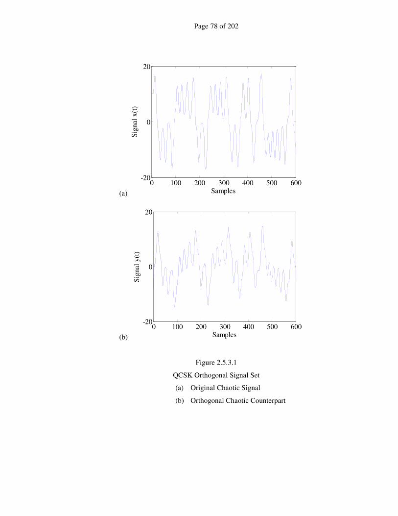
Page 78 of 202
(a)
0 100 200 300 400 500 600-20
0
20
Samples
Sig
nal
x(t
)
(b)
0 100 200 300 400 500 600-20
0
20
Samples
Sig
nal
y(t
)
Figure 2.5.3.1
QCSK Orthogonal Signal Set
(a) Original Chaotic Signal
(b) Orthogonal Chaotic Counterpart

Page 79 of 202
Derivation 2.5.3.1
______________________________________________________________________
Consider a signal on a closed interval ],0[)( Tttx ∈∀ , which is generated by a
chaotic system and is modified by removing the mean value so that it is a zero
mean process, that is
∫ =
T
dttxT
0
0)(1
(2.5.3.2)
then a Fourier expansion of this signal can be expressed as
∑∞
=
+=
1
)sin()(
m
mm tmftx φω (2.5.3.3)
where T/2πω = and 00 =f
Define the average power of this signal as
∫=
T
x dttxT
P
0
2 )(1
(2.5.3.4)
which because of the following properties of sinusoidal functions
∫ −+−+T
nnmm dttnftmfT 0
)sin()sin(1
βφωαφω
)cos(2
1 2 βα −= mf ∀ nm =
0= ∀ nm ≠ (2.5.3.5)
can be expressed as
∑∞
=
=
1
2
2
1
m
mx fP (2.5.3.6)
Now to derive a signal that is orthogonal to )(tx . Apply a Hilbert Transform to
the signal with a phase shift of 2/π . This can be achieved by taking a Fourier
Transform of the signal and rotating the positive frequencies by 2/π and the
negative ones by 2/π− . Finally inverting gives the transformed function
)2
sin()(
1
∑∞
=
++=
m
mm tmftyπ
φω (2.5.3.7)

Page 80 of 202
(a) (b)
then
∫ =⇔⊥
T
dttytxT
yx
0
0)()(1
(2.5.3.8)
it follows then that
∫∫ =⇔=
TT
yx dttyT
dttxT
PP
0
2
0
2 )(1
)(1
(2.5.3.9)
______________________________________________________________________
Consider now two possible maximally separated constellations of signals that consist of
an addition of a proportion of each orthogonal signal. These can be represented on an
Argand diagram shown in figure (2.5.3.1) and the encoding values set out in table
(2.5.3.1)
Figure 2.5.3.2
Maximal Separation Quadrature Constellations
Existing on a Two Dimensional Hypersphere:
(a) Symbol encoding contains the reference signal whereas
(b) Encodes all symbols.

Page 81 of 202
Table 2.5.3.1
______________________________________________________________________
Symbol 0 1 2 3
1 0 -1 0 (a) c
0 1 0 -1
2/1 2/1− 2/1− 2/1 (b) c
2/1 2/1 2/1− 2/1−
Maximal separation quadrature constellation encoding symbol maps
______________________________________________________________________
Each symbol can be represented by a complex number as
ir jccc += (2.5.3.10)
Orthogonality is assured in the complex plane and its analogy can therefore be
represented along the real time axis, if the two complimentary signals are orthogonal;
that is
)()()( tyctxcts ir += (2.5.3.11)
this is the message signal for each symbol in the message.
At the receiver the symbols can be retrieved by determining the coefficients of each
individual orthogonal component by using the two correlation integrals
Result 2.5.3.1
______________________________________________________________________
∫=
T
xr dttxts
TPc
0
)()(1
(2.5.3.12)
∫=
T
yi dttyts
TPc
0
)()(1
(2.5.3.13)
______________________________________________________________________
The derivation of the result is outlined below

Page 82 of 202
Derivation 2.5.3.2
______________________________________________________________________
∫∫ +=
T
ir
T
dttxtyctxcdttxts
00
)())()(()()(
∫ +=
T
ir dttxtyctxc
0
2 )()()(
TPc xr= (2.5.3.14)
∫∫ +=
T
ir
T
dttytyctxcdttyts
00
)())()(()()(
∫ +=
T
ir dttxtyctytxc
0
2 )()()()(
TPc yi= (2.5.3.15)
______________________________________________________________________
2.6 Observer Methods
The principal idea behind the Drive Response technique, of section (2.3.1), is that the
receiver is driven to reconstruct a subset of the states of a chaotic system that reflects
that of the transmitter producing them. The system is then a coherent one, and some
form of comparison technique can then detect the signal by synchronization or non-
synchronization of a single system as in sections (2.3.2) and (2.3.3); or the
synchronization of one system of many as in section (2.3.4). This can really be
considered as a class of Observer method, which is well understood for linear systems.
Various other techniques have been proposed [25][36] based on the control systems
theory of constructing observers. The basic idea is simple to state. The receiver needs to
contain an observer to reconstruct the state of the transmitter within the receiver. In [36]
a linear time invariant error mechanism is developed which has stated necessary and
sufficient conditions to ensure that the state error vector asymptotically diminishes to

Page 83 of 202
zero. This method proves to be more robust than a simple Drive Response
Synchronization technique.
The basic concept behind other forms of observer based methods rely on various forms
of the description below. Consider the transmitter system
xc
xfx
Tty
tt
=
=
)(
))(()(& (2.6.1)
where )(ty is a combination of the states of the chaotic system, which is to be
transmitted, and will be used to observe and recreate the state vector in the receiver.
Consider now the receiver system
xc
mxfx
ˆ)(ˆ
))()(ˆ())(ˆ()(ˆ
Tty
tytytt
=
−+=& (2.6.2)
Now define an error vector as
xxe −= ˆ (2.6.3)
Then it follows that
xxe &&& −= ˆ (2.6.4)
and combining equations (2.7.1) to (2.7.4) the dynamical equation of the error is
determined as a function of the observer vector
emcxfxfe T+−= )()ˆ(& (2.6.5)
To design an observer vector m the non-linear element needs to be considered. Firstly
the non-linear term of this equation can be linearized at the current state value x
and becomes
)()(
)()()ˆ( xfex
xfxfxfxf −
∂
∂+=−
ex
xf
∂
∂=
)( (2.6.6)
if equation (2.7.3) is rearranged for the estimate vector as
exx +=ˆ (2.6.7)
Page 84 of 202
and substituting (2.7.6) and (2.7.7) into (2.7.5) yields the following observer dynamical
error system
emcx
xfe
+
∂
∂= T)(
& (2.6.8)
This is again simply an asymptotic estimator with a non-linear element. Now providing
that the m vector is chosen to give the observer stable eigenvalues [51-53] with any
state x within the strange attractor of the chaotic system, then the state of the receiver
will synchronize with that of the transmitter. If the real parts of the eigenvalues are set
to more negative values than the existing system values, then the response time, noise
rejection properties and the robustness of the observer are improved [53].
2.7 Feedback Methods
Feedback control of the state of the receiver is primarily used to synchronize the
receiver with the transmitter when they are dissimilar due to modelling inaccuracies or
some other consideration such as security. Methods using nonlinear control techniques
can be used to make the transmitter and the receiver synchronize, even when dissimilar
which has value for improving system robustness. An example of one method is shown
here.
Consider the following nonlinear dynamical system that represents the transmitter. The
state and transmission signal equations are
xc
xfx
Tty
tt
=
=
)(
))(()(& (2.7.1)
where the )(ty is the transmitted signal. Now represent the receiver as a model of the
transmitter, with an integral observer as described in section (2.6), and a model of the
dissimilar system with a control vector which is yet to be determined, that is
xc
mxfx
ˆ)(ˆ
))()(ˆ())(ˆ()(ˆ
Tty
tytytt
=
−+=& (2.7.2)
and
Page 85 of 202
)())(()( ttt uzgz +=& (2.7.3)
where the control is given by the vector )(tu , the estimate of the transmitter state is
given by )(ˆ tx and the dissimilar system vector function )(zg has a state )(tz at time t.
The purpose of the control vector )(tu is to drive the error between the estimate of the
transmitter state )(ˆ tx and the dissimilar system state )(tz to zero.
Now define an error vector as
zxe −= ˆ (2.7.4)
Then it follows that
zxe &&& −= ˆ (2.7.5)
and combining equations (2.7.2) to (2.7.5) the dynamical equation of the error is
determined as a function of the control vector
uzgxfe −−= )()ˆ(& (2.7.6)
now
ez
zfzfezfxf
∂
∂+=+=
)()()()ˆ( (2.7.7)
which implies that
uez
zfzεe −
∂
∂+=
)()(& (2.7.8)
where the error between the two systems is given by
)()()( zgzfzε −= (2.7.9)
The determination of u is complex and dependent on the system equations. The control
vector u is designed to ensure that the Lyapunov stability criteria for the system are
assured. That is a Lyapunov error function defined as
0)(21 ≥= eee TV (2.7.10)
is positive semi definite and that its first derivative is negative definite, that is
0)( <= eee TV && (2.7.11)

Page 86 of 202
The drawbacks of this approach are firstly that the receiver requires an observer to
reconstruct the state x of the transmitter and secondly, that the design of the controller
cannot be considered in a generic manner but must be carefully tailored to a specific
system [28]. The advantages are a robust nature of the synchronization with good noise
rejection, especially when the systems are very similar.
2.8 Detectability
Methods of detection of signals transmitted using chaotic processes have been
proposed. One method [29] introduced by G. Perez and H. A. Cereira presumes a
chaotic transmission stream using the Lorenz attractor. It revisits ideas proposed
originally by Lorenz himself. It is possible to construct a one-dimensional return map
by considering the local maxima and minima that one of the states returns to. If nX is
the value of )(tx when it reaches its local maxima and mY is the value of )(tx when it
reaches its local minima, then the return maps of 1+nX versus nX and 1+mY versus mY
can be constructed. These maps are almost one-dimensional, and from manipulations of
these maps, information about the signal being transmitted can be extracted; since the
signal is recognised as a particular chaotic transmitter in a certain transmission mode.
Other methods that are based on the underlying nature of the attractors in the systems
are referred to in [29-33].
The detectability of FM-DCSK type systems is inherent in the way that they repeat the
basic chaotic signal in a number of combinations for each frame of the reference and
message bearing parts of their transmission. By autocorrelating the incoming signal,
over an extended period, the repetitiveness of the signal will become apparent by
repeated impulse like forms in the correlation function. This easily reveals the time
frame and allows further analysis of the message bearing signal sequences. This is a
valid method of increasing the dimensionality, and hence the transmission efficiency of
the communication scheme, but it requires further encryption of the message to ensure
its security.

Page 87 of 202
2.9 Summary
From the above sections it has been shown that using synchronisation techniques for
communications schemes alone is prone to noise rejection problems, and that any
system based purely on this form of communication is not usually robust. There is a
wealth of further work here which, especially for the covert communications fields,
could be exploited. The internal states of the nonlinear systems of both the drive and
response systems are possibly capable of conveying multilevel messages with only one
physically visible communication signal and this would present a great advantage and is
truly worthy of further research. However for the purposes of this thesis the type of
scheme chosen will be the reference signal approach which is vastly more robust and
more able to handle noisy environments. The aim will be to improve the transmission
rate and efficiencies of discrete time multilevel communication schemes, in real time,
by exploiting orthogonal signal sets in a number of novel architectures.
Page 88 of 202
Chapter 3
An Orthogonal Chaotic Vector Shift Keying
Communication Scheme
3.1 Introduction
In this chapter a number of new multidimensional transmission encoding schemes are
described. Firstly, the limitations of two dimensional schemes with increased
transmission efficiency are explored in section (3.2) and then the problems of extending
the Fourier expansion method, used in QCSK and described in section (2.4.3), to higher
dimensions are highlighted in section (3.3). Consequently, the problem is restated in a
multidimensional way. The theory of a multidimensional scheme is then derived in
section (3.4) and in section (3.5) a simple robust method of obtaining a
multidimensional orthogonal signal set is advanced. A number of encoding and
decoding schemes are then presented with their system architectures described in
section (3.6). And finally, the Bit Error Rate (BER), probability problem and the
problems of signal characterization; and the signal to noise ratio effects on the BER, are
derived in a new and novel way for each of the encoding schemes described in sections
(3.7) to (3.9).

Page 89 of 202
(a) (b)
3.2 Limitations of Two Dimensional Schemes with Increased
Transmission Efficiency
Firstly, the limitations of Quadrature Chaos Shift Keying (QCSK) are explored. This
method can clearly be developed into an M-ary type constellation method, allowing the
transmission of more symbols, thus improving the symbol transmission efficiency. This
is illustrated below in figure (3.2.1).
Figure 3.2.1
M-ary Two Dimensional Constellations
(a) ‘8’ Symbol ‘3’ Bit and (b) ‘16’ Symbol ‘4’ Bit Representations
A disadvantage of this method is, that all of the points on the constellation lie on a fixed
radius circle that is normally represented on the complex plane. Large numbers of
symbols require an equally large number of points on the fixed circle, which becomes
crowded, and hence gives rise to potential misinterpretation on decoding; this scheme is
therefore not robust. One way to avoid this is to vary both the amplitude of the symbol
representations as well as the phase. This is known as Quadrature Amplitude
Modulation (QAM) illustrated in figure (3.2.2).
This form of variation of grid type or circle radius type constellation gives rise to signal
amplitude variation. This is not desirable, as this would make the signals more easily
detectable by varying the power of the transmitted signals. QCSK, QAM and other
types of communication constellation scheme are usually represented on the complex

Page 90 of 202
(a) (b)
plane. This is largely an historical convenience based on Fourier analysis representation
and not a true reflection of the nature of the employed signals. The complex
representation is derived from complex analysis, which employs the inherent
orthogonality of the sine and cosine functional representation, on the complex plane. If
symbols are represented within a higher dimensional space, then the apparent
dependence on inherent orthogonality can be discarded; the effective separation
between the symbols can be increased and the effects of noise reduced.
Figure 3.2.2
QAM Type Two Dimensional Constellations
(a) ‘16’ Symbol ‘4’ Bit Grid and (b) ‘16’ Symbol ‘4’ Bit Circular
3.3 Orthogonal Properties of Extended Dimension Fourier Generated
Signals
The Fourier Expansion used in QCSK is detailed in Derivation (2.4.3.1), but consider
here, the summary for illustration purposes. Consider the chaotic signal )(tx defined on
the closed interval ],0[ T , which has had the mean value removed, and thus can be
considered as a zero mean process over the interval.
Now suppose that it will admit to a Fourier expansion of infinite length that is
∑∞
=
+=
1
)sin()(
k
kk tkftx φω (3.3.1)
where T
πω
2= and 00 =f
and the following sinusoidal properties are true
Page 91 of 202
dttmftkfT
I mmk
T
k )sin()sin(1
0
βϕωαϕω −+−+= ∫
0=I for mk ≠
)cos(2
2
αβ −= kfI for mk = (3.3.2)
For )(ty to be orthogonal to )(tx over the interval then
0)()(1
0
=∫ dttytxT
T
(3.3.3)
Now as )(tx is given as an infinite Fourier Expansion, then there are an infinite number
of signals orthogonal to it derived by applying a phase shift of 2
π± to each sinusoidal
element of )(tx . So
∑∞
=
±+=
1
)2
sin()(
k
kk tkftyπ
φω (3.3.4)
In the definition of integral I consider 0=α and 2
πβ ±=
then
dttmftkfT
I mmk
T
k )2
sin()sin(1
0
πϕωϕω m++= ∫
0=I for mk ≠
0)2
cos(2
2
=±=πkfI for mk = (3.3.5)
So 0=I in all cases and therefore )(ty is orthogonal to )(tx .
Consider now an approximation to )(tx derived from a limited sum of q sinusoidal
elements, that is
∑=
+=
q
k
kk tkftx
1
)sin()( φω (3.3.6)
It follows that there are q2 signals orthogonal to the )(tx approximation expressed as
follows
∑=
++=
q
k
kkp kpFtkfty
1
)2
),(sin()(π
φω (3.3.7)
Page 92 of 202
where ]2,1[ qp ∈ and ),( kpF is a notional function of p and k that takes the values
1± and varies as a Gray scale from )()( 1 tyty pp +→ so that only one phase change
takes place at each step in the entire expansion.
Consider then the question: Are the )(typ ∀ ]2,1[ qp ∈ signals generated from )(tx
mutually orthogonal. To show this is not so, consider any two derived signals )(tyi and
)(ty j so
dttytyT
IT
ji∫=0
)()(1
(3.3.7)
dtkjFtkfkiFtkfT
IT
q
k
kkkk∫ ∑=
++++=0
1
)2
),(sin()2
),(sin(1 π
ϕωπ
ϕω (3.3.8)
Since all other terms vanish then
( )∑=
−=
q
k
k kjFkiFfI
1
2
2),(),(cos
2
1 π (3.3.9)
∑=
=
q
k
k kGfI
1
2 )(2
1 (3.3.10)
where 1)( ±=kG
Clearly, it is possible to find a limited set of mutually orthogonal functions, but it is
dependent on the values of eachkf and as each signal set is different being generated
from a chaotic sequence; it is not trivial to find a set ],1[ qkfk ∈∀ which drives
equation (3.3.10) to zero. So, generally it is true, that all the )(tyk signals are not
mutually orthogonal.
Therefore, it can be concluded that the Fourier expansion method of orthogonal signal
generation is not suitable for dimensions greater than m=2.
If it is feasible to separate the problem from complex analysis, the problem can be
restated as finding sets of mutually orthogonal signals. The combination of these signals
can, in a similar way to QCSK, be extended to much greater information capacity and
hence transmission efficiency. QCSK introduces this idea, but is immediately
constrained, by the use of the Fourier expansion and Hilbert Transform methods.
Page 93 of 202
Presented is a method of overcoming this problem, by the use of a system of orthogonal
sequences, derived by using the Gram-Schmidt orthonormalization method.
3.4 Theoretical Analysis
In the QCSK approach, the key requirement is the generation of a signal orthogonal to
the chaotic reference signal. This requirement is met by assuming that the reference
signal )(tx over the interval ],0[ Tt ∈ has zero mean and will admit to a Fourier
expansion which, as shown in section (2.4.3), results in a possible set of orthogonal
signals )(ty . Once a set of two basis signals is generated, a variety of signalling schemes
can be created based on constellations formed on the complex plane, see figure
(2.4.3.1). Specifically each symbol is represented as table (2.4.3.1)
ir jccc += (3.4.1)
and associated with it is the symbolic modulated signal
)()()( tyctxcts ir += (3.4.2)
Recovery of these signals in the receiver is achieved using the two correlation integrals
∫=
T
xr dttxts
TPc
0
)()(1
(3.4.3)
∫=
T
xi dttyts
TPc
0
)()(1
(3.4.4)
Where
y
TT
x PdttyT
dttxT
P === ∫∫0
2
0
2 )(1
)(1
The derivation of which is shown in result (2.4.3.1). The number of symbols can be
increased into M-ary constellations, with varying amplitudes and phases in the complex
plane, as in figures (3.2.1) and (3.2.2) but this inherent two dimensionality of the QCSK
approach decreases its potential noise rejection properties when large symbol
constellations are considered.

Page 94 of 202
Consider now a system, with an m dimensional constellation, that relies on m different
mutually orthogonal signals, which actually form an orthonormal basis of functions
)(tui ∀ ],1[ mi ∈ .
Derivation 3.4.1
______________________________________________________________________
As with the QCSK scheme, the message can be encoded using these orthogonal
functions by combining them linearly using the value of the encoding coefficients.
This can now be represented as
)(...)()()()( 332211 tuctuctuctucts mm++++= (3.4.5)
which in vector function notation becomes
cu )()( tts T= (3.4.6)
where
)](,),(),(),([)( 321 tutututut mT
K=u (3.4.7)
and
],...,,[ 21 mT ccc=c (3.4.8)
this is the message signal for each symbol in our message.
At the receiver the symbols can be retrieved by determining the coefficients of
individual orthogonal components by using the m correlation integrals
∫=
T
ii
i dttutsTP
c
0
)()(1
∀ ],1[ mi ∈ (3.4.9)
∫=
T
ii dttuT
P
0
2 )(1
(3.4.10)
or from (3.4.6) to (3.4.8)
∫∫ =
T
T
T
dtttdttst
00
)()()()( cuuu (3.4.11)
Therefore this can be written in concise vector notation as
∫∫−
=
TT
Tdttstdttt
0
1
0
)()()()( uuuc (3.4.12)
______________________________________________________________________

Page 95 of 202
This will work with any set of signals if they are independent. If there is no noise
present, the signal sets are orthogonal and the inversion is simplified by the matrix
being diagonal. However in the presence of noise, the inversion can influence the noise
rejection characteristics of decoding. Noise rejection can be improved by discarding non
diagonal terms because they are perceived to have been generated by noise. The scheme
of signal transmission here is irrelevant to the above derivation. The signals can be
transmitted simultaneously on multiple channels or contiguously on one channel.
3.5 Generation of Orthogonal Signal Sets
The generation of a set of m orthogonal signals is required; we can approach this
problem by first considering an n dimensional space. Any point p can be represented by
an n dimensional vector that is a linear sum of the set of orthonormal basis vectors iu
where ni R∈u and ],1[ ni ∈ .
Therefore we can write
nnpppp uuuup ++++= ...332211 (3.5.1)
Where ],1[ nipi ∈∀ are real coefficients.
Now consider a subset of size m of these basis vectors that describe an m dimensional
subspace within the n dimensional space. Further consider, the set of vectors describing
some hypersurface s within this m dimensional subspace.
mmcccc uuuus ++++= ...332211 (3.5.2)
Here p and nR∈s and nm ≤ . The size of n is explored in chapter 4 but is an order of
magnitude greater in size than m for noise rejection purposes. This can be seen as
analogous to equation (3.4.5) in section (3.4), excepting that the summation is in terms
of real vectors, and not real functions of t. The real vectors iu can be obtained from the
real functions )(tui by the following process. That is Tniii uu ][ 1 L=u and
))1(( iiji tjuu +−= τ where ],1[ nj ∈ , itmi ],,1[∈ is the initial time at the point of
sampling each vector and τ is the sampling period. These can be arranged into a matrix
][ 1 muuU L= where mn
R×∈U . For a practical consideration any real function )(tui
can generate a vector of signal values iu by sampling. Conversely, the real signal
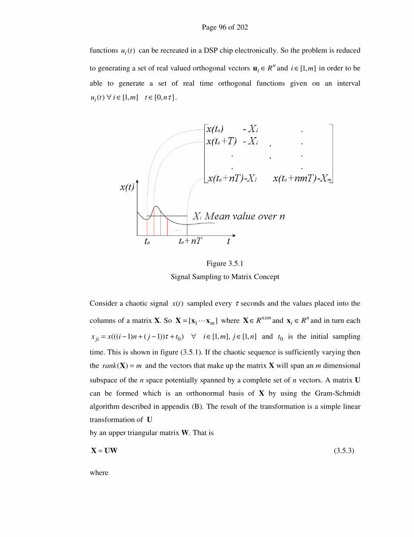
Page 96 of 202
functions )(tui can be recreated in a DSP chip electronically. So the problem is reduced
to generating a set of real valued orthogonal vectors ni R∈u and ],1[ mi ∈ in order to be
able to generate a set of real time orthogonal functions given on an interval
],0[],1[)( τntmitui ∈∈∀ .
Figure 3.5.1
Signal Sampling to Matrix Concept
Consider a chaotic signal )(tx sampled every τ seconds and the values placed into the
columns of a matrix X. So ][ 1 mxxX L= where nxmR∈X and ni R∈x and in turn each
],1[],,1[)))1()1((( 0 njmitjnixx ji ∈∈∀+−+−= τ and 0t is the initial sampling
time. This is shown in figure (3.5.1). If the chaotic sequence is sufficiently varying then
the mrank =)(X and the vectors that make up the matrix X will span an m dimensional
subspace of the n space potentially spanned by a complete set of n vectors. A matrix U
can be formed which is an orthonormal basis of X by using the Gram-Schmidt
algorithm described in appendix (B). The result of the transformation is a simple linear
transformation of U
by an upper triangular matrix W. That is
UWX = (3.5.3)
where

Page 97 of 202
mT IUU = (3.5.4)
and W can be found as
XUUWUTT = (3.5.5)
So given equation (3.5.4) it follows that
XUWT= (3.5.6)
However, finding this transformation is unnecessary if the Gram-Schmidt algorithm is
used; it is specified here because it will be needed for signal characterization in section
(3.8).
Consider now the independence of the columns of X , and how this relates to the
potential number of bits of precision that the signal set values may be in error. In order
to determine if the signal set is ‘good’ enough for transmission, an estimate of the ‘bits’
in precision error ( eB ) can be determined from the matrix 2-norm condition number
nC as
( )ne CB 2log∝ (3.5.7)
where the condition number is given as
( ) ( )iinC λλ min/max= ∀ [ ]mii ,∈ (3.5.8)
here the iλ represent the eigenvalues of the symmetric matrix XXT and iλ are the
singular values of X. If eB is larger than the bit precision of the signal set values that
are to be transmitted the matrix, and hence the signal set, can be rejected. With the
condition number sufficiently small the U matrix can be separated into a set of vectors
iu ∀ [ ]mii ,∈ , which can be seen as samples of a set of continuous signals with zero
mean over the time interval ],0[ τnt ∈ and average powers of n/1 . These can now be
encoded according to an encoding scheme, power balanced and transmitted. Power
balancing here means that each signal sequence has the same average power. This is
achieved by post multiplying the signal relevant matrix by an appropriate diagonal
square matrix P. This is discussed in chapter 4.

Page 98 of 202
3.6 System Architectures and Encoding and Decoding Schemes
In this section there are three different system architectures presented, with their
associated encoding and decoding schemes. The first two can be considered as ‘m
symbol’ type schemes, where a series of m symbols are transmitted for each set of
derived orthogonal signals. The first scheme exhibits extremely good noise rejection
without any real dependence on the nature of the chaotic process chosen. Whereas, the
noise rejection of the second scheme has a greater dependence on the type of chaotic
process. It is presented only as a precursor to understanding the signal characterization
described in section (3.8) and as an introduction to the third transmission scheme. The
final scheme has the same inherent requirement as the second scheme, namely to choose
the chaotic process carefully, but it is a novel persistent updating method giving rise to
much greater transmission efficiency.
3.6.1 Direct ‘m Symbol’ ‘U’ Scheme
Figure 3.6.1.1
‘U’ Scheme - Direct ‘m Symbol’ Transmission System Architecture
Consider the mn × signal matrix X produced by taking nm samples of the chaotic
process. Where each set of n samples has the mean value removed thus leaving each
vector of the matrix X as samples of a zero mean process. Now an mn × orthonormal
matrix U is generated from it using the Gram-Schmidt process detailed in appendix (B).
The matrix U is multiplied by a diagonal power balancing matrix P to produce a matrix
Q as in equation (3.6.1.1) before being streamed. Streaming is transmitting each
element of each column of the Q matrix in turn over the communication channel. The

Page 99 of 202
choice of the diagonal matrix P is arbitrary but specifying it in terms of a signal to noise
power ratio will become significant in section (3.8) and (3.9).
Therefore
UPQ = (3.6.1.1)
A set of symbol bearing transmittable signal sequences S is generated by encoding the
columns of Q with an encoding vector for each symbol to be represented, that is
QCSQcs =⇔∈∀= ],1[ miii (3.6.1.2)
where
],...,,[ 21 mcccC = (3.6.1.3)
and ic represents the ith
symbol of m. The matrix S is now transmitted in the same way
as matrix Q. This method of ‘m symbol’ transmission is chosen to increase the
transmission efficiency. The transmitted sequence for each symbol is only n samples
long whereas the completed transmitted reference Q matrix is m times longer. The
simple solution is to transmit m symbols with m encoded sequences for each reference
sequence. Each encoded sequence can represent m2 states or symbols with each
transmission set of reference and encoded sequences it is possible to transmit a possible
( )mm2 different symbols by shifting in a bit register m bits left for each of the m
sequences as shown in table (3.6.1.1).
______________________________________________________________________
m Bits m Bits < < m Bits
m )1( −m 1
Table 3.6.1.1
Shift register of m bits for each of the m sequences.
______________________________________________________________________
The potential set of encoding vectors ]2,1[ mj j ∈∀c is chosen from an encoding map
mm
R2×∈C which is calculated as
],...,,[)2(21 mcccC = (3.6.1.4)
Page 100 of 202
( )m
j mj
µbc
−−⋅=
)1(2 (3.6.1.5)
where the jc vectors lie on an m dimensional hypersphere of unit radius within the n
space; mm R∈µ is a vector ],1[1 mii ∈∀=µ and ]2,1[)1( mjj ∈∀−b is the bit pattern
function converting a bit pattern to an ordered vector, that is
[ ]Tmbbbj L21)( =b (3.6.1.6)
and
],1[}1,0{21
1
mibbj i
m
i
imi ∈∀∈+= ∑
=
− (3.6.1.7)
Example 3.6.1.1
______________________________________________________________________
For the system dimension 4=m the twelfth encoding vector represents the
number 11, that is 12=j . This can be represented by the bit pattern ( )1101
which can be interpreted as 01232121202111 ×+×+×+×= which maps directly
to
Tj ]1101[)1( =−b (3.6.1.8)
Now if T]1111[4 =µ it follows that
( )4
)11(2 412
µbc
−⋅=
[ ]T21
21
21
21 −= (3.6.1.9)
______________________________________________________________________
Consider now the method of decoding the received signals. The equivalent of the
correlation integral in equation (3.4.12), is a least squares approximation of the
encoding vector, given a noisy received signal matrix S . If the signal of the thi column
is considered then
iii εQcs σ+= (3.6.1.10)
where
UPQ = (3.6.1.11)

Page 101 of 202
the noise term contains iε which is Gaussian White noise process with a zero mean and
a unit variance, that is { } 0ε =iE and { } nE iTi =εε and P is a diagonal power balancing
matrix. In the following equations, the notation indicates a variable derived from
received signal data and the ^ indicates an estimated value. Now the signal estimate for
a particular symbol represented by a column of the received signals matrix S is given
by
ii cQs ˆˆ = (3.6.1.12)
expressing the error between the received signal vector and the estimated one as
iii sse ˆ−= (3.6.1.13)
and forming a squared error sum as
iT
ii ee=η (3.6.1.14)
now minimize iη with respect to the estimate of the encoding vector ic so
T
i
iTi 0
c
ee =
∂
∂
ˆ2 (3.6.1.15)
from equations (3.6.1.12) and (3.6.1.13)
Qc
e−=
∂
∂
i
i
ˆ (3.6.1.16)
Therefore (3.6.1.15) can be rearranged, incorporating equations (3.6.1.12) and
(3.6.1.13) as
0cQsQ =− )ˆ( iiT (3.6.1.17)
And finally forming an estimate of the encoding vector by rearranging (3.6.1.17) as
[ ] iTT
i sQQQc1
ˆ−
= (3.6.1.18)
This is the least squares discrete equivalent of the correlation integral given by equation
(3.4.12). Now if all m sequences are considered then this equation becomes
[ ] SQQQCTT 1
ˆ−
= (3.6.1.19)
where
[ ]mcccC ˆ,...,ˆ,ˆˆ21= and [ ]msssS ,...,, 21= (3.6.1.20)
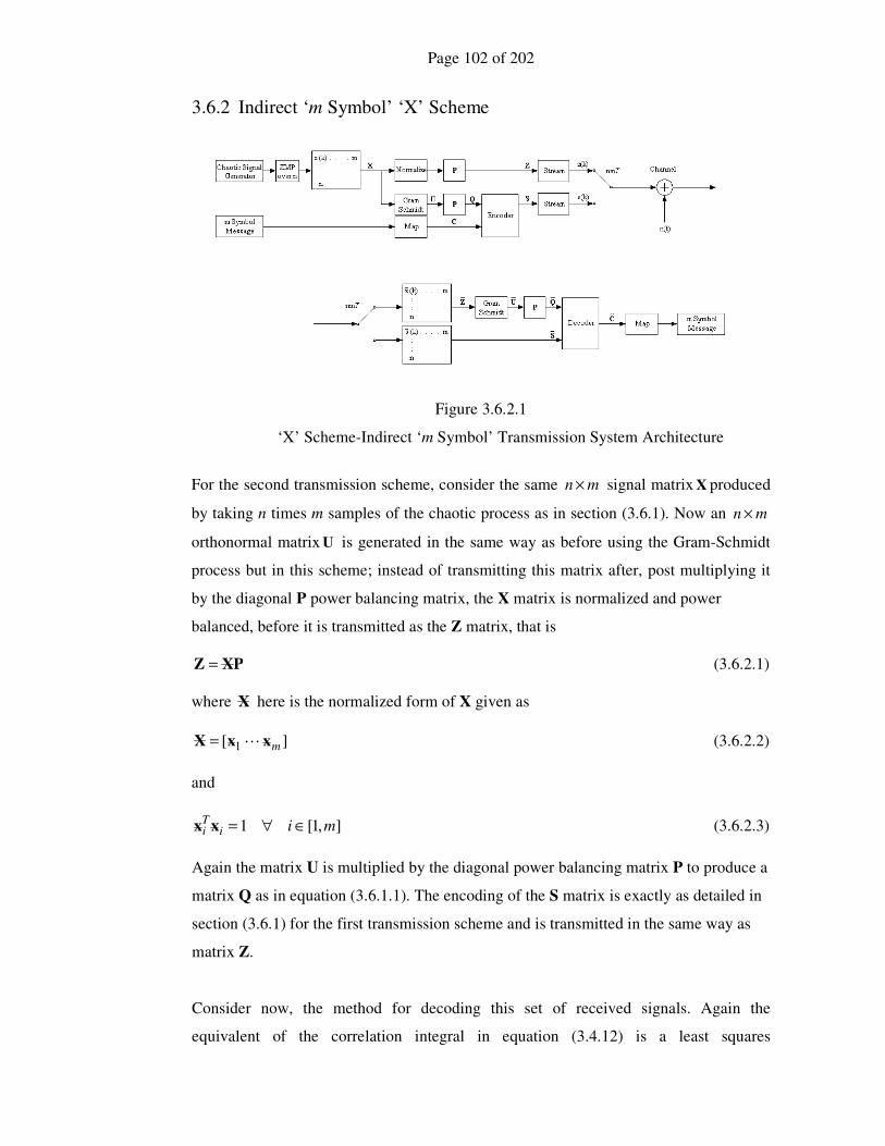
Page 102 of 202
3.6.2 Indirect ‘m Symbol’ ‘X’ Scheme
Figure 3.6.2.1
‘X’ Scheme-Indirect ‘m Symbol’ Transmission System Architecture
For the second transmission scheme, consider the same mn × signal matrix X produced
by taking n times m samples of the chaotic process as in section (3.6.1). Now an mn ×
orthonormal matrix U is generated in the same way as before using the Gram-Schmidt
process but in this scheme; instead of transmitting this matrix after, post multiplying it
by the diagonal P power balancing matrix, the X matrix is normalized and power
balanced, before it is transmitted as the Z matrix, that is
PXZ = (3.6.2.1)
where X here is the normalized form of X given as
][ 1 mxxX L= (3.6.2.2)
and
],1[1 miiTi ∈∀=xx (3.6.2.3)
Again the matrix U is multiplied by the diagonal power balancing matrix P to produce a
matrix Q as in equation (3.6.1.1). The encoding of the S matrix is exactly as detailed in
section (3.6.1) for the first transmission scheme and is transmitted in the same way as
matrix Z.
Consider now, the method for decoding this set of received signals. Again the
equivalent of the correlation integral in equation (3.4.12) is a least squares

Page 103 of 202
approximation of the encoding vector given a noisy received signal matrix S . This
differs from the first scheme since the received matrix is not the noise contaminated U
matrix but a non-orthogonal signal set received as matrix Z . Both U and Q matrices
can be formed by using the Z matrix via the Gram-Schmidt process. If the signal of the
thi column is considered then the equivalent of equations (3.6.1.10) and (3.6.1.11)
becomes
iii εcQs σ+= (3.6.2.4)
and
PUQ = (3.6.2.5)
in the same way, the noise term contains iε which is Gaussian White noise with a zero
mean and a unit variance, that is { } 0ε =iE , { } nE iTi =εε and P is a diagonal power
balancing matrix. As before, equations with the notation indicate a variable derived
from received signal data and the ^ indicates an estimated value. The estimation of the
encoding vectors is the same as in section (3.6.1) equations (3.6.1.12) to (3.6.1.20),
excepting that due to the Gram-Schmidt process now residing in both the transmitter
and the receiver a slight variation occurs. Consider the estimate equation for a single
symbol
[ ] iTT
i sQQQc1
ˆ−
= (3.6.2.6)
now substitute into this equation the equation (3.6.2.5) to give
[ ] iTTTT
i sUPPUUPc1
ˆ−
= (3.6.2.7)
because the U matrix was generated by the Gram-Schmidt process it follows that
mT
IUU = (3.6.2.8)
and as the P matrix is diagonal equation (3.6.2.7) becomes
iT
i sUPc1ˆ −= (3.6.2.9)
if all m sequences are considered then this equation becomes
SUPCT1ˆ −= (3.6.2.10)
where
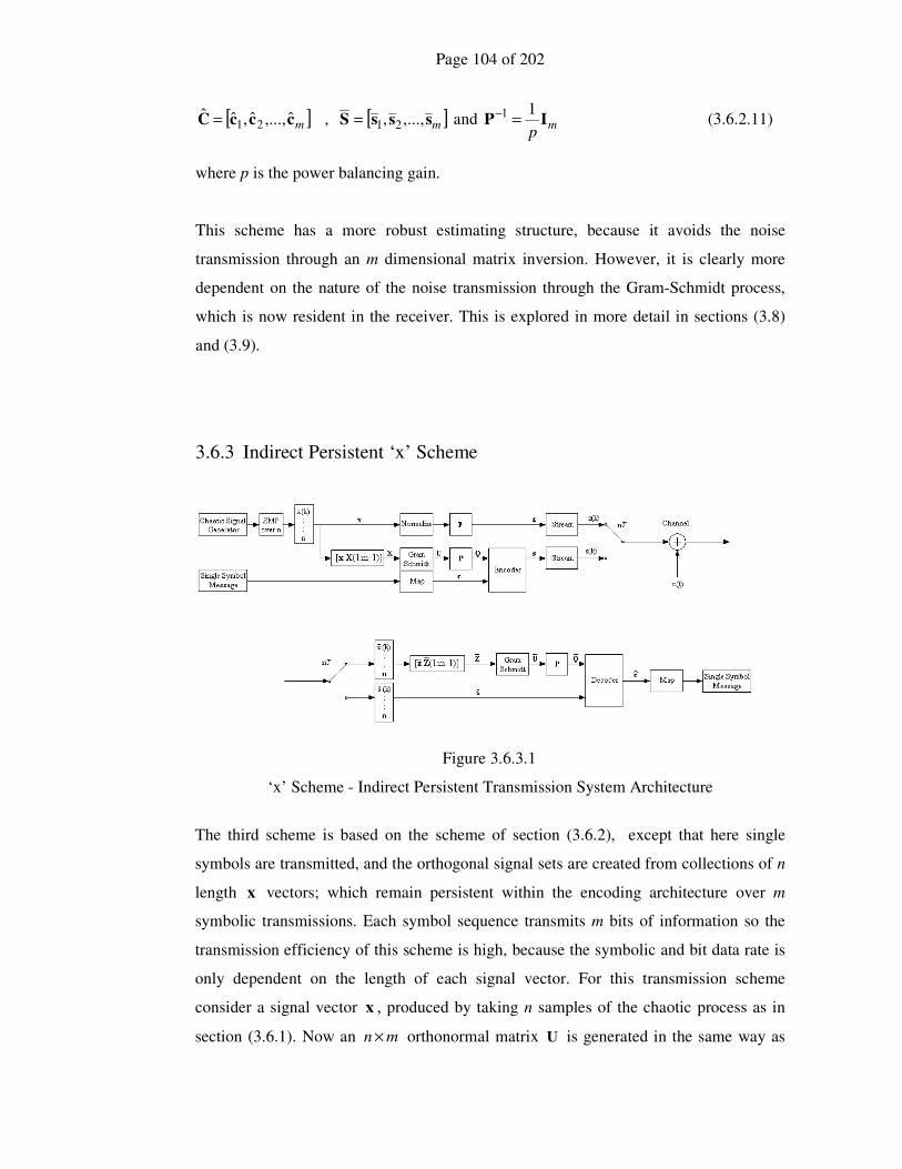
Page 104 of 202
[ ]mcccC ˆ,...,ˆ,ˆˆ21= , [ ]msssS ,...,, 21= and m
pIP
11 =− (3.6.2.11)
where p is the power balancing gain.
This scheme has a more robust estimating structure, because it avoids the noise
transmission through an m dimensional matrix inversion. However, it is clearly more
dependent on the nature of the noise transmission through the Gram-Schmidt process,
which is now resident in the receiver. This is explored in more detail in sections (3.8)
and (3.9).
3.6.3 Indirect Persistent ‘x’ Scheme
Figure 3.6.3.1
‘x’ Scheme - Indirect Persistent Transmission System Architecture
The third scheme is based on the scheme of section (3.6.2), except that here single
symbols are transmitted, and the orthogonal signal sets are created from collections of n
length x vectors; which remain persistent within the encoding architecture over m
symbolic transmissions. Each symbol sequence transmits m bits of information so the
transmission efficiency of this scheme is high, because the symbolic and bit data rate is
only dependent on the length of each signal vector. For this transmission scheme
consider a signal vector x , produced by taking n samples of the chaotic process as in
section (3.6.1). Now an mn × orthonormal matrix U is generated in the same way as

Page 105 of 202
before, using the Gram-Schmidt process, but in this scheme the required X matrix is
made up from m successive x signal vectors, and instead of transmitting this matrix,
after post multiplying it by the diagonal P power balancing matrix, the x vector is
normalized and power balanced before it is transmitted as the z vector. That is
pxz = (3.6.3.1)
where x here is the normalized form of x and
1=xxT (3.6.3.2)
A new X matrix is created after each x vector is sampled as
][ 1,, −= mnmn XxX (3.6.3.3)
A new U matrix is generated every n samples and this is multiplied by the diagonal
power balancing matrix P to produce a matrix Q as in equation (3.6.1.1). It is now
necessary only to encode a single symbol represented by an s vector as
Qcs = (3.6.3.4)
and this is transmitted in that same way as the z vector.
Consider now the method for decoding each received signal vector. Again the
equivalent of the correlation integral in equation (3.6.2.6) is a least squares
approximation of the encoding vector given a noisy received signal vector s . This now
differs from the second scheme, since a Z needs to be created in order to decode the
signals, in the same way as the second scheme in section (3.6.2). This is created as
][ 1,, −= mnmn ZzZ (3.6.3.5)
now both U and Q matrices can be formed by using the Z matrix via the Gram-
Schmidt process. The decoding is equivalent to the second scheme yielding the
following
iT
i sUPc1ˆ −= (3.6.3.6)
where
mp
IP11 =− (3.6.3.7)
where p is the power balancing gain.

Page 106 of 202
This scheme has the same robust estimating structure as the second scheme, because it
avoids the noise transmission through an m dimensional matrix inversion, and it has the
same dependency on the nature of the noise transmission through the Gram-Schmidt
process. The cyclic transmission efficiency is increased and is scaleable with the
dimension m, without any noise or time penalties.
3.7 BER Probability Formulation
To find the Bit Error Rate (BER), as a function of the number of samples n for each bit
and the signal power to noise power ratio snrP of the system, the following probability
formulation will enable a simple method of BER calculation to be developed in section
(3.9). The BER is considered as the probability that a singular transmitted bit is decoded
incorrectly in the receiver. This can be considered as a function of the probability of the
estimate of the encoding vector lying outside its permitted region. Consider then the
probability of getting all the bits correct that is
)(1)( µµ EPCP −= (3.7.1)
where )( µEP is the probability of any error and µ is the number of symbols, hence if
b is the number of bits representing µ symbols then
b2=µ (3.7.2)
The probability of the thi symbol being correct is
bi CPCP )()( µ= (3.7.3)
this gives the probability of a symbol error as
)(1)( ii CPEP −= (3.7.4)
Now this is equivalent to the Bit Error Rate so from equations (3.7.1) to (3.7.4)
b EPBER )(11 µ−−= (3.7.5)
3.8 Signal Characterization
In this section, the effects of noise transmitted through the various processes in the
estimators are considered. As the third transmission scheme, the ‘Indirect Persistent x
Scheme’ described in section (3.6.3) is essentially the same, in a noise transmission
sense, as the ‘Indirect m Symbol X Scheme’ described in section (3.6.2); this section

Page 107 of 202
has two parts, one looking at the relatively simple characterization of the ‘Direct m
Symbol U Scheme’ of section (3.6.1), and the more complex ideas of the ‘Indirect m
Symbol X Scheme’.
3.8.1 Direct ‘m Symbol’ ‘U’ Scheme
The transmittable signal matrix U, derived from the Gram-Schmidt process, can be
characterized by considering it to be expressed as a series of column vectors with the
same power. As U consists of an orthonormal basis over a limited m dimensional span
of the n space it can be expressed as
=
− mmn
m
,0
IU (3.8.1.1)
If a scheme uses this matrix as the reference, then it would be power balanced before
transmission, and by definition each column would have the same power. The signals
are derived from an arbitrary chaotic process, and for the purposes of characterization,
can be aggregated in this way. This is clearly independent of any process and is
notionally derived in this form to ensure it has the correct properties principally that
mT IUU = (3.8.1.2)
Before transmission, this matrix is multiplied by a diagonal power balancing matrix to
yield a transmittable matrix Q. When this matrix is contaminated in the transmission
channel by zero mean Gaussian White noise with a variance of 2σ the received signal
matrix can be expressed as
EQQ σ+= (3.8.1.3)
Where E is a matrix of Gaussian White noise signals of unit variance with the same
dimensions as Q.
Now the estimator matrix is constructed as follows
EUPQ σ+= (3.8.1.4)
In order to complete this characterization we need to consider the diagonal power
balancing matrix P in terms of the Power to Signal Noise Ratio snrP .
Define the snrP as
Page 108 of 202
2
2
σ
x=snrP (3.8.1.4)
where 2
x is the power of an arbitrary signal vector x and can be considered as the
norm of the length n vector given as
xxx T
n
12= (3.8.1.5)
Now we require that
2xqq n
T = (3.8.1.6)
that is, it is required that the transmitted vectors have a nominal power 2
x and the total
energy content increases linearly as the vector length n. For the scheme being
considered
],1[22 mipp iTii
Ti ∈∀== uuqq (3.8.1.7)
Combining equations (3.8.1.4), (3.8.1.6) and (3.8.1.7) yields
snrnPp σ= (3.8.1.8)
and therefore
msnrnP IP ⋅= σ (3.8.1.9)
This finally allows the desired characterization of Q as
+
⋅=
−
E0
IQ
mmn
msnrnP
,
σ (3.8.1.10)
Likewise the ith
symbol signal vector can be characterized in the same way, that is
εQcs σ+= ii ],1[ mi ∈∀ (3.8.1.11)
where ε is an n length vector of Gaussian White noise signals of unit variance.
Substituting equations (3.8.1.1) and (3.8.1.9) into this equation (3.8.1.11) gives
+
⋅=
−
εc0
Is i
mmn
msnri nP
,
σ ],1[ mi ∈∀ (3.8.1.12)
Page 109 of 202
These results give characterizations of the received signal vectors is and the received
reference matrix Q . They have a simple structure for the message bearing element and
have simple Gaussian white noise elements which will allow simple analysis of the
noise propagation through the entire communications scheme.
3.8.2 Indirect ‘m Symbol’ ‘X’ Scheme
The transmittable signal matrix Z is received in a noise contaminated form as Z . A
noise contaminated orthonormal set of signal vectors U can be derived using the Gram-
Schmidt process and an equivalent Q matrix can be found as
PUQ = (3.8.2.1)
The U matrix has properties that can be characterized, by considering it to be expressed
as a series of column vectors with the same power. As U consists of an orthonormal
basis over a limited m dimensional span of the n space it can be expressed as
=
− mmn
m
,0
IU (3.8.2.2)
This signal aggregation is valid, but does not describe the errors induced by the
presence of noise on the Gram-Schmidt process. This is clearly independent of any
process and is notionally derived in this form to ensure it has the correct properties
principally that
mT IUU = (3.8.2.3)
A simple way of characterizing the effect of the Gram-Schmidt process is to consider
how the transmitted matrix Z is constructed. The Z matrix is a power balanced version
of a normalized set of signal vectors generated by a chaotic process. As such they are
inherently not orthogonal, and can be considered as the result of an upper triangular
linear transformation of an orthonormal basis, as described in section (3.5) equations
(3.5.3) to (3.5.6), (3.6.2.1) and (3.8.1.9), that is
PXZ =
UW⋅= snrnPσ (3.8.2.4)
So finally the Q matrix can be characterized in the following way if )(ZG is the Gram-
Schmidt matrix function and W is upper triangular with
Page 110 of 202
],1[1 miiTi ∈∀=ww (3.8.2.5)
it follows that
( )( )EUWGU +⋅= snrnPσ (3.8.2.6)
So finally
( )( )EUWGQ +⋅⋅= snrsnr nPnP σσ (3.8.2.7)
the standard deviation constant σ within the Gram-Schmidt matrix function has no
effect here, since it merely changes the component vector lengths and not their
relationship to one another. Therefore this can be written as
( )EUWGQ +⋅⋅= snrsnr nPnPσ (3.8.2.8)
Likewise, as before, the ith
symbol signal vector can be characterized in the same way as
in section (3.8.1), that is
εQcs σ+= ii ],1[ mi ∈∀ (3.8.2.9)
ε is an n length vector of Gaussian White noise signals of unit variance and so
substituting equations (3.8.1.1) and (3.8.1.9) into this equation gives
+
⋅=
−
εc0
Is i
mmn
msnri nP
,
σ ],1[ mi ∈∀ (3.8.2.10)
3.9 Signal to Noise Calculations
In order to evaluate the performance of these transmission schemes against other
schemes, a novel way is presented for producing Bit Error Rate results using the
probability formulation of section (3.7) and the signal characterization of section (3.8).
The results differ for each scheme and are presented in the next two sections.

Page 111 of 202
3.9.1 Direct ‘m Symbol’ ‘U’ Scheme
The ith
symbol encoding vector estimate can be expressed as follows
iTT
i sQQQc 1][ˆ −= ∀ ],1[ mi ∈ (3.9.1.1)
Now the estimate can be expressed in terms of the noise on the transmission channel
and the original idealised symbol encoding vector by substituting equations (3.8.1.10)
and (3.8.1.12) into (3.9.1.1), that is
+
⋅=
−
E0
IQ
mmn
msnrnP
,
σ (3.9.1.2)
and
+
⋅=
−
εc0
Is i
mmn
msnri nP
,
σ ],1[ mi ∈∀ (3.9.1.3)
which yields
L
1
,,
ˆ
−
−−
+
⋅
+
⋅= E
0
IE
0
Ic
mmn
msnr
T
mmn
msnri nPnP σσ
+
⋅
+
⋅
−−
εc0
IE
0
Ii
mmn
msnr
T
mmn
msnr nPnP
,,
σσL
( ) L1
,, )(−
+++= EEEEI Tmmmm
Tsnrmsnr nPnP
( )εEεcEc Tmimm
Tsnrisnr nPnP +++ )( ,L ],1[ mi ∈∀ (3.9.1.4)
Here mm,E is the first m rows of the E matrix and mε is the first m elements of ε .
From this equation the probability formulation of Bit Error Rate, outlined in section
(3.7), can now be calculated. If a typical value for the encoding vector ic is used in a
simulation, then whenever a simulated estimate of ic is calculated outside this region,
the number of failures is summed over a range of snrP values and a waterfall type curve
is produced accordingly. The results of this kind of analysis can be seen in chapter 4.
Page 112 of 202
The result here is constructed using the power of the signal to noise ratio snrP , whereas
most of the literature quotes the equations and results in terms of the ‘energy per bit
divided by the noise power’, that is 0N
Eb . This depends on the bit transmission rate,
which in turn, is dependent on the structure of the different signal sequences. snrP is
independent of transmission structure. If the transmission bit rate rB is known and the
energy is spread over the reference and the signal sequences then
r
snrb
B
P
N
E
τ20
= (3.9.1.5)
For orthogonal minimal constellations the bit rate, including the reference sequence
time is given by
τn
mBr
2= (3.9.1.6)
where τ is the sampling time of the system.
Substituting equation (3.9.1.6) into (3.9.1.5) and rearranging gives
⋅=
0N
E
n
mP b
snr (3.9.1.7)
Finally then equation (3.9.1.4) becomes
L
1
,,
00
)(ˆ
−
++
+
= EEEEIc T
mmmmTb
mb
iN
Em
N
Em
++
+
εEεcEc T
mimmTb
ib
N
Em
N
Em )( ,
00
L ],1[ mi ∈∀ (3.9.1.8)
3.9.2 Indirect ‘m Symbol’ ‘X’ Scheme
Again the ith
symbol encoding vector estimate can be expressed as follows
iTT
i sQQQc 1][ˆ −= ∀ ],1[ mi ∈ (3.9.2.1)
As before the estimate can be expressed in terms of the noise on the transmission
channel, and the original idealised symbol encoding vector by substituting equations

Page 113 of 202
(3.8.2.8) and (3.8.2.10) into (3.9.2.1), that is
+
⋅⋅=
−
EW0
IGQ
mmn
msnrsnr nPnP
,
σ
U⋅= snrnPσ (3.9.2.2)
and
+
⋅=
−
εc0
Is i
mmn
msnri nP
,
σ ],1[ mi ∈∀ (3.9.2.3)
which yields
( ) ( ) L
1
ˆ−
⋅⋅= UUc snr
T
snri nPnP σσ
( )
+
⋅⋅
−
εc0
IU i
mmn
msnr
T
snr nPnP,
σσL
+
=
−
εc0
IU
snri
mmn
mT
nP
1
,
],1[ mi ∈∀ (3.9.2.4)
where
+
⋅=
−
EW0
IGU
mmn
msnrnP
,
(3.9.2.5)
The results again can be presented in terms of the probability formulation of Bit Error
Rate outlined in section (3.7) and the ‘energy per bit over the noise power’ 0N
Eb yielding
+
=
−
εc0
IUc
0
,
1ˆ
N
Em b
immn
mTi ],1[ mi ∈∀ (3.9.2.6)
Page 114 of 202
3.10 Summary
In this chapter, the limitations of two dimensional M-ary type schemes have been
highlighted and further to this, the failure of extending Fourier expansion methods to
produce orthogonal signal sets has been demonstrated. A method has then been derived
to produce orthogonal signal sets utilizing the Gram-Schmidt orthonormalization
process and a number of different system architectures have been presented which
increase transmission efficiency and information density over a communication
channel. These schemes have then been characterized to allow an analysis of the noise
transmission through them and analyses of their performance under varying noisy
conditions have been presented.

Page 115 of 202
Chapter 4
Simulation Case Study
4.1 Introduction
A case study for the schemes proposed in chapter 3 is now presented for a dimension of
4=m . This dimension has been chosen, because it allows a clear demonstration of the
advantages of using these schemes, whilst not presenting information that may be too
confusing or complex for the purposes of illustration. The chapter is divided into two
parts, section (4.2) presents a set of transmission simulations, for all of the proposed
schemes, where simulated real time random messages are transmitted and received with
Gaussian White noise added in the communication channel. Illustrated, are the actual
transmitted and the received messages and the errors in the decoding of the information,
due to the noise in the channel. The next section (4.3) presents the ‘Bit Error Rates’
(BER) in terms of the ‘Power Signal to Noise Ratio’ ( snrP ) and the ‘Energy per Bit
divided by the Noise Power’
0N
Eb . It is required that for each estimator, the probability
of the vector estimate lying outside its permitted region is determined, that is
]2,1[)())(ˆ( mk
mk kEPRP ∈∀=∉ µcc (4.1.1)
be found, this is equivalent to the BER. Varying the noise matrices and vectors
randomly over a large number of simulation runs produces the following results shown,
in each of the figures of sections (4.3.1) and (4.3.2), for snrP and 0N
Eb . Plots of BER for

Page 116 of 202
(a) DCSK, (b) QCSK 16 symbol constellation and (c) OCVSK 16 symbol methods are
presented. The data rates for the selected examples areτn2
1,
τn
2 and
τn
2 respectively,
where n is the number of samples in the reference and the message bearing part of the
signal and τ is the sampling time. The generalized data rate for the orthogonal scheme
is τn
m
2 where m is the scheme dimension. Although the bit efficiency of the QCSK 16
symbol constellation is as good as the OCVSK 16 scheme, the BER is much worse
indicating a clear advantage to the orthogonal scheme.
A further comparison is presented, showing that the Orthogonal Chaotic Vector Shift
Keying (OCVSK) methods have BER characteristics equivalent to Differential Chaos
Shift Keying (DCSK), when the reference signals are orthogonal. The BER for the
DCSK scheme and the OCVSK 16 scheme, has a dimensionally larger number of
samples with the same BER, but the OCVSK 16 scheme has four times the data rate.
However, as the signal references become more non-orthogonal, represented by non
diagonal values of the signal characteristic matrix W described in section (3.5), the BER
graphs diverge quite markedly. This is illustrated in figures (4.3.1.2), (4.3.2.1.2),
(4.3.2.2.2) and (4.3.2.3.2).
The chaotic system used here is the Lorenz system described in section (2.1.3). The
advantages of this system are that it is simple, and has sufficiently chaotic behaviour for
the purposes of demonstrating chaotic communication methods; but has characteristics
that illustrate the problems that systems with a degree of periodicity can cause
orthogonally oriented communication schemes. The systems equations used for these
results are
zxyz
xzyrxy
yxx
βα
α
σσα
+=
−−=
+−=
&
&
&
(4.1.1)
where 28=r , 10=σ and 3/8=β . The constant α can be chosen to suit the sampling
time that the particular system requires. For the following simulations 1=α , all
sampling times are assumed to be units of the chosen sample period and the first state
)(tx is used as the signal to be sampled.
Page 117 of 202
4.2 Transmission Simulations
4.2.1 Direct ‘m Symbol’ ‘U’ Scheme
Figure (4.2.1.1) shows a series of graphs illustrating how the various stages of the
scheme in section (3.6.1) are processed. Graph (a) shows the matrix X of zero mean
sampled sequences generated from the chaotic process. Graph (b) shows the
orthonormal basis matrix sequences U generated from the matrix X which in turn, when
multiplied by the diagonal power balancing matrix P, generates the Q matrix in graph
(c). The Q matrix sequences are then streamed and transmitted. When these sequences
are resampled at the receiver they have been contaminated by noise, with a power to
signal noise ratio of unity, as shown in graph (d). The Q matrix is now encoded with m
symbol vectors to generate the S matrix of graph (e), and this is streamed and received
in the same way as the Q matrix, to yield the noise contaminated S matrix in graph (f).
These graphs show the diverse and spread spectrum nature of the chaotic signals, which
make up the signals for all of the transmission schemes, and one of the principal reasons
why these types of schemes are particularly able to reject banded limited noise.
A set of transmitted ‘sixteen’ bit messages, represented by four separate ‘four’ bit
groups, is shown in figure (4.2.1.2) graphs (a) and (b). Graphs (c) and (d) show the
decoded messages in both ‘sixteen’ bit form and as four ‘four’ bit groups. They show
the received messages delayed by nm time samples, and the following two graphs (e)
and (f), demonstrates that there is zero error between the transmitted and the received
message sequence at a snrP of unity when the time delay is accounted for. This clearly
illustrates the noise rejection properties of using orthogonal sequences as reference
signals.
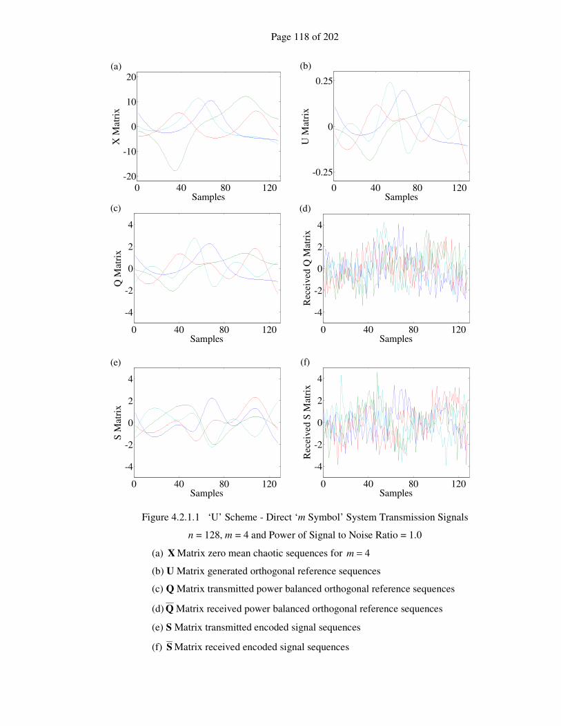
Page 118 of 202
0 40 80 120
-20
-10
0
10
20(a)
Samples
X M
atr
ix
0 40 80 120
-0.25
0
0.25
(b)
Samples
U M
atri
x
0 40 80 120
-4
-2
0
2
4
(c)
Samples
Q M
atri
x
0 40 80 120
-4
-2
0
2
4
(d)
Samples
Rec
eiv
ed Q
Mat
rix
0 40 80 120
-4
-2
0
2
4
(e)
Samples
S M
atri
x
0 40 80 120
-4
-2
0
2
4
(f)
Samples
Rec
eiv
ed S
Mat
rix
Figure 4.2.1.1 ‘U’ Scheme - Direct ‘m Symbol’ System Transmission Signals
n = 128, m = 4 and Power of Signal to Noise Ratio = 1.0
(a) X Matrix zero mean chaotic sequences for 4=m
(b) U Matrix generated orthogonal reference sequences
(c) Q Matrix transmitted power balanced orthogonal reference sequences
(d) Q Matrix received power balanced orthogonal reference sequences
(e) S Matrix transmitted encoded signal sequences
(f) S Matrix received encoded signal sequences
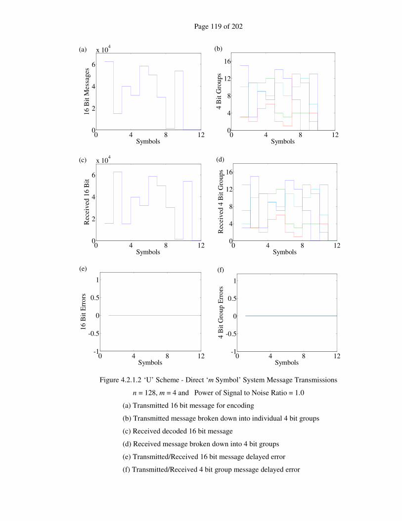
Page 119 of 202
0 4 8 120
2
4
6
x 104
(a)
Symbols
16
Bit
Mess
ages
0 4 8 120
4
8
12
16
(b)
Symbols
4 B
it G
roups
0 4 8 120
2
4
6
x 104
(c)
Symbols
Rec
eiv
ed 1
6 B
it
0 4 8 120
4
8
12
16
(d)
Symbols
Rec
eived
4 B
it G
roups
0 4 8 12-1
-0.5
0
0.5
1
(e)
Symbols
16
Bit
Err
ors
0 4 8 12-1
-0.5
0
0.5
1
(f)
Symbols
4 B
it G
roup
Err
ors
Figure 4.2.1.2 ‘U’ Scheme - Direct ‘m Symbol’ System Message Transmissions
n = 128, m = 4 and Power of Signal to Noise Ratio = 1.0
(a) Transmitted 16 bit message for encoding
(b) Transmitted message broken down into individual 4 bit groups
(c) Received decoded 16 bit message
(d) Received message broken down into 4 bit groups
(e) Transmitted/Received 16 bit message delayed error
(f) Transmitted/Received 4 bit group message delayed error

Page 120 of 202
4.2.2 Indirect ‘m Symbol’ ‘X’ Scheme
For the next scheme figure (4.2.1.2) shows a series of graphs illustrating the various
stages of the scheme described in section (3.6.2). Graph (a) shows the matrix X of zero
mean sampled sequences generated from the chaotic process. Graph (b) shows the
orthonormal basis matrix sequences U generated from the matrix X which in turn, when
multiplied by the diagonal power balancing matrix P, give rise to the Q matrix which is
used for encoding the signals sequence matrix S shown in graph (e). In this scheme the
references are generated from the X matrix by normalizing it and power balancing it
with the diagonal P matrix to generate the Z matrix in graph (c), they are then streamed
and transmitted. When these sequences are resampled at the receiver they have been
contaminated by noise, with a power to signal noise ratio of unity, as shown in graph
(d). The Q matrix is now encoded with m symbol vectors to generate the S matrix of
graph (e), and this is streamed and received in the same way as the Z matrix, to yield
the noise contaminated S matrix in graph (f). There are advantages to this scheme
which will be more fully realised in the next transmission scheme, but the prime
disadvantage here is that the Z matrix sequences are not orthogonal, and are thus more
liable to noise induced errors on decoding. This illustrates why the sequences should be
chosen carefully via the matrix conditioning method described in section (3.5).
The same set of transmitted ‘sixteen’ bit messages, represented by four separate ‘four’
bit groups, are shown in figure (4.2.2.2) graphs (a) and (b). Graphs (c) and (d) show the
decoded messages in both ‘sixteen’ bit form and as four ‘four’ bit groups. They show
the received messages delayed by nm time samples and the following two graphs, (e)
and (f), demonstrates that there are errors between the transmitted and the received
message sequence at a snrP of unity, when the time delay is accounted for. This clearly
illustrates that the noise rejection properties are impaired by using non orthogonal
sequences as references signals. This is modelled and illustrated in section (4.3) when
the BER of these schemes is considered.

Page 121 of 202
0 40 80 120
-20
-10
0
10
20(a)
Samples
X M
atr
ix
0 40 80 120
-0.25
0
0.25
(b)
Samples
U M
atri
x
0 40 80 120
-4
-2
0
2
4
(c)
Samples
Z M
atr
ix
0 40 80 120
-4
-2
0
2
4
(d)
Samples
Rec
eiv
ed
Z M
atri
x
0 40 80 120
-4
-2
0
2
4
(e)
Samples
S M
atri
x
0 40 80 120
-4
-2
0
2
4
(f)
Samples
Rec
eiv
ed S
Mat
rix
Figure 4.2.2.1 ‘X’ Scheme - Direct ‘m Symbol’ System Transmission Signals
n = 128, m = 4 and Power of Signal to Noise Ratio = 1.0
(a) X Matrix zero mean chaotic sequences for 4=m
(b) U Matrix generated orthogonal reference sequences
(c) Z Matrix transmitted power balanced reference sequences
(d) Z Matrix received power balanced reference sequences
(e) S Matrix transmitted encoded signal sequences
(f) S Matrix received encoded signal sequences

Page 122 of 202
0 4 8 120
2
4
6
x 104
(a)
Symbols
16
Bit
Mess
ages
0 4 8 120
4
8
12
16
(b)
Symbols
4 B
it G
roup
s
0 4 8 120
2
4
6
x 104
(c)
Symbols
Rec
eived
16
Bit
0 4 8 120
4
8
12
16
(d)
Symbols
Rec
eiv
ed 4
Bit
Gro
up
s
0 4 8 12-2
0
2x 10
4
(e)
Symbols
16 B
it E
rrors
0 4 8 12
-8
0
8
(f)
Symbols
4 B
it G
roup
Err
ors
Figure 4.2.2.2 ‘X’ Scheme - Direct ‘m Symbol’ System Message Transmissions
n = 128, m = 4 and Power of Signal to Noise Ratio = 1.0
(a) Transmitted 16 bit message for encoding
(b) Transmitted message broken down into individual 4 bit groups
(c) Received decoded 16 bit message
(d) Received message broken down into 4 bit groups
(e) Transmitted/Received 16 bit message delayed error
(f) Transmitted/Received 4 bit group message delayed error

Page 123 of 202
4.2.3 Indirect Persistent ‘x’ Scheme
The next four figures (4.2.3.1) to (4.2.3.4) illustrate the results of simulating the scheme
described in section (3.6.3) for two values of 0.1=snrP and 0.10=snrP . The simulation
uses the same chaotic sequences, that the first two schemes used, that have not been
enhanced by the matrix conditional method of sequences selection. Hence the noise
rejection evident in the scheme simulated in section (4.2.1), and the inability of the
scheme in section (4.2.2) to demonstrate the same noise rejection, is only restored by an
increase in the snrP value. Graph (a) shows a single vector sequence x, and graph (b)
shows the persistent matrix X of zero mean sampled sequences, generated from the
chaotic process. Graph (c) shows the orthonormal basis matrix sequences U, generated
from the matrix X which in turn, when multiplied by the diagonal power balancing
matrix P, give rise to the Q matrix which is used for encoding the signals sequence
vector s shown in graph (e). In this scheme, the references are generated from the x
vector by normalizing and power balancing it with the power value p, to generate the
streamed and transmitted z vector. When these sequences are resampled at the receiver,
they have been contaminated by noise, and assembled into a persistent Z matrix as
shown in graph (d). The Q matrix is now encoded with a single symbol vector to
generate the s vector of graph (e), and this is streamed and received in the same way as
the z vector, to yield the noise contaminated s vector in graph (f). The main advantage
to this scheme is, that for each reference sequence and encoded sequence, there are m
bits of information transmitted, which is one symbol representing m bits.
The same set of transmitted and received ‘four’ bit messages are shown in figures
(4.2.3.3) and (4.2.3.4) graphs (a) and (b). Graph (c) demonstrates that, there are errors
between the transmitted and the received message sequence with both snrP values, when
the time delay is accounted for. The first m signals are always in error. as the persistent
matrices are not fully populated until four message sequences have been transmitted.
This illustrates, as with all communication schemes, a need for some form of preamble
before real information can be transmitted. The noise rejection can again be increased
by the careful selection of the chaotic sequences outlined in section (3.5). The limits of
this scheme are the clearly the noise rejection due to the sequence length n, the chaotic
sequence conditional selection and the dimension chosen for m, which is investigated
and optimally selected in chapter 5.

Page 124 of 202
0 40 80 120
-20
-15
-10
-5
0
5
10
15
20(a)
Samples
x V
ecto
r
0 40 80 120
-20
-15
-10
-5
0
5
10
15
20(b)
Samples
X M
atri
x
0 40 80 120
-0.25
0
0.25
(c)
Samples
U M
atr
ix
0 40 80 120-5
-2.5
0
2.5
5(d)
Samples
Rec
eiv
ed Z
Mat
rix
0 40 80 120-3
-1.5
0
1.5
3(e)
Samples
s V
ecto
r
0 40 80 120-3
-1.5
0
1.5
3(f)
Samples
Rec
eived
s V
ecto
r
Figure 4.2.3.1 Indirect Persistent ‘x’ Scheme System Transmission Signals
n = 128, m = 4 and Power of Signal to Noise Ratio = 1.0
(a) Transmitter zero mean chaotic sequences x
(b) Persistent chaotic sequences X
(c) Generated orthogonal reference sequences U
(d) Received power balanced reference sequences Z
(e) Transmitted encoded signal sequence s
(f) Received encoded signal sequence s
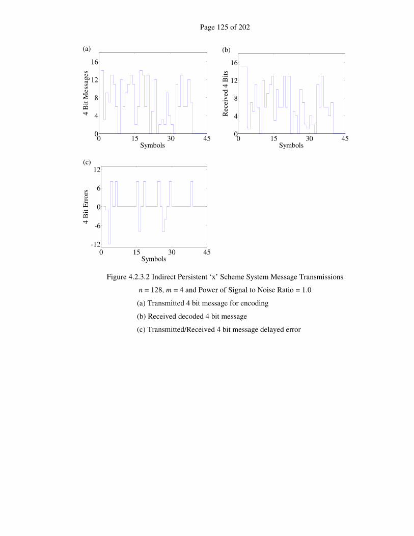
Page 125 of 202
0 15 30 450
4
8
12
16
(a)
Symbols
4 B
it M
ess
ages
0 15 30 450
4
8
12
16
(b)
Symbols
Rec
eived
4 B
its
0 15 30 45-12
-6
0
6
12(c)
Symbols
4 B
it E
rro
rs
Figure 4.2.3.2 Indirect Persistent ‘x’ Scheme System Message Transmissions
n = 128, m = 4 and Power of Signal to Noise Ratio = 1.0
(a) Transmitted 4 bit message for encoding
(b) Received decoded 4 bit message
(c) Transmitted/Received 4 bit message delayed error
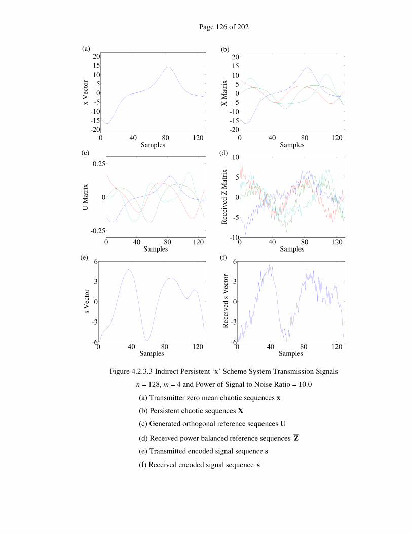
Page 126 of 202
0 40 80 120
-20
-15
-10
-5
0
5
10
15
20(a)
Samples
x V
ecto
r
0 40 80 120
-20
-15
-10
-5
0
5
10
15
20(b)
Samples
X M
atri
x
0 40 80 120
-0.25
0
0.25
(c)
Samples
U M
atr
ix
0 40 80 120-10
-5
0
5
10(d)
Samples
Rece
ived Z
Matr
ix
0 40 80 120-6
-3
0
3
6(e)
Samples
s V
ecto
r
0 40 80 120-6
-3
0
3
6(f)
Samples
Rec
eiv
ed s
Vec
tor
Figure 4.2.3.3 Indirect Persistent ‘x’ Scheme System Transmission Signals
n = 128, m = 4 and Power of Signal to Noise Ratio = 10.0
(a) Transmitter zero mean chaotic sequences x
(b) Persistent chaotic sequences X
(c) Generated orthogonal reference sequences U
(d) Received power balanced reference sequences Z
(e) Transmitted encoded signal sequence s
(f) Received encoded signal sequence s

Page 127 of 202
0 15 30 450
4
8
12
16
(a)
Symbols
4 B
it M
essa
ges
0 15 30 450
4
8
12
16
(b)
Symbols
Rec
eiv
ed 4
Bit
s
0 15 30 45-12
-6
0
6
12(c)
Symbols
4 B
it E
rrors
Figure 4.2.3.4 Indirect Persistent ‘x’ Scheme System Message Transmissions
n = 128, m = 4 and Power of Signal to Noise Ratio = 10.0
(a) Transmitted 4 bit message for encoding
(b) Received decoded 4 bit message
(c) Transmitted/Received 4 bit message delayed error

Page 128 of 202
4.3 BER Simulations
4.3.1 Direct ‘m Symbol’ ‘U’ Scheme
-20 -10 0 10 2010
-4
10-3
10-2
10-1
100(a)
Psnr[dB]
BE
R D
CS
K8 Samples
32 Samples
128 Samples
0 5 10 15 2010
-4
10-3
10-2
10-1
100(b)
Eb/No[dB]
BE
R D
CS
K
8 Samples
32 Samples
128 Samples
-20 -10 0 10 2010
-4
10-3
10-2
10-1
100(c)
Psnr[dB]
BE
R Q
CS
K 1
6
8 Samples
32 Samples
128 Samples
0 5 10 15 2010
-4
10-3
10-2
10-1
100(d)
Eb/No[dB]
BE
R Q
CS
K 1
68 Samples
32 Samples
128 Samples
-20 -10 0 10 2010
-4
10-3
10-2
10-1
100(e)
Psnr[dB]
BE
R O
CV
SK
16
8 Samples
32 Samples
128 Samples
0 5 10 15 2010
-4
10-3
10-2
10-1
100(f)
Eb/No[dB]
BE
R O
CV
SK
16
8 Samples
32 Samples
128 Samples
Figure 4.3.1.1 Direct ‘m’ Symbol ‘U’ Scheme
BER v snrP and 0N
Eb Comparison Plot for ]128,32,8[∈n samples
(a) and (b) DCSK : BER versus snrP and 0N
Eb
(c) and (d) QCSK 16 Symbol Constellation : BER versus snrP and 0N
Eb
(e) and (f) OCVSK 16 : BER versus snrP and 0N
Eb
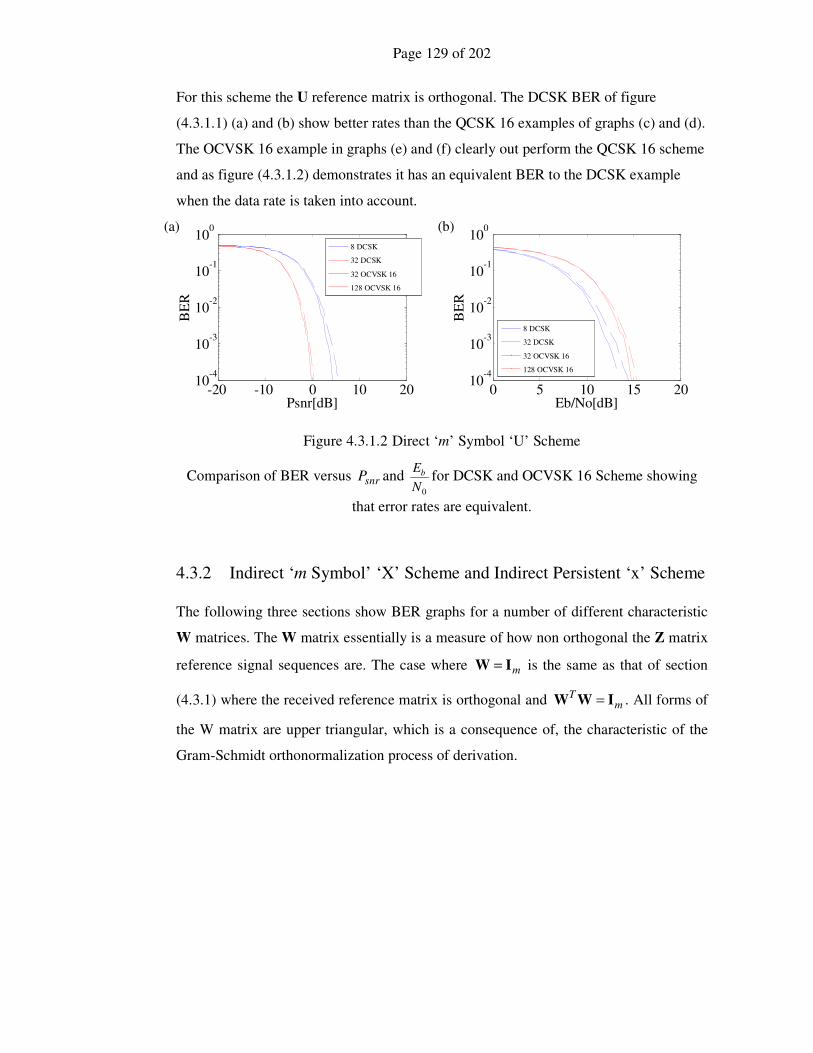
Page 129 of 202
For this scheme the U reference matrix is orthogonal. The DCSK BER of figure
(4.3.1.1) (a) and (b) show better rates than the QCSK 16 examples of graphs (c) and (d).
The OCVSK 16 example in graphs (e) and (f) clearly out perform the QCSK 16 scheme
and as figure (4.3.1.2) demonstrates it has an equivalent BER to the DCSK example
when the data rate is taken into account.
-20 -10 0 10 2010
-4
10-3
10-2
10-1
100(a)
Psnr[dB]
BE
R
8 DCSK
32 DCSK
32 OCVSK 16
128 OCVSK 16
0 5 10 15 2010
-4
10-3
10-2
10-1
100(b)
Eb/No[dB]
BE
R
8 DCSK
32 DCSK
32 OCVSK 16
128 OCVSK 16
Figure 4.3.1.2 Direct ‘m’ Symbol ‘U’ Scheme
Comparison of BER versus snrP and 0N
Eb for DCSK and OCVSK 16 Scheme showing
that error rates are equivalent.
4.3.2 Indirect ‘m Symbol’ ‘X’ Scheme and Indirect Persistent ‘x’ Scheme
The following three sections show BER graphs for a number of different characteristic
W matrices. The W matrix essentially is a measure of how non orthogonal the Z matrix
reference signal sequences are. The case where mIW = is the same as that of section
(4.3.1) where the received reference matrix is orthogonal and mT IWW = . All forms of
the W matrix are upper triangular, which is a consequence of, the characteristic of the
Gram-Schmidt orthonormalization process of derivation.
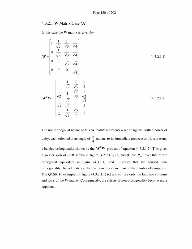
Page 130 of 202
4.3.2.1 W Matrix Case ‘A’
In this case the W matrix is given by
=
4
1000
4
1
3
100
4
1
3
1
2
10
4
1
3
1
2
11
W (4.3.2.1.1)
=
12
3
2
1
2
1
2
31
3
2
3
1
2
1
3
21
2
1
2
1
3
1
2
11
WWT (4.3.2.1.2)
The non-orthogonal nature of this W matrix represents a set of signals, with a power of
unity, each oriented at an angle of 4
π radians to its immediate predecessor. It represents
a banded orthogonality shown by the WWT
product of equation (4.3.2.1.2). This gives
a greater span of BER shown in figure (4.3.2.1.1) (e) and (f) for snrP over that of the
orthogonal equivalent in figure (4.3.1.1), and illustrates that the banded non-
orthogonality characteristic can be overcome by an increase in the number of samples n.
The QCSK 16 examples of figure (4.3.2.1.1) (c) and (d) use only the first two columns
and rows of the W matrix. Consequently, the effects of non-orthogonality become more
apparent.

Page 131 of 202
-20 -10 0 10 2010
-4
10-3
10-2
10-1
100(a)
Psnr[dB]
BE
R D
CS
K
8 Samples
32 Samples
128 Samples
0 5 10 15 2010
-4
10-3
10-2
10-1
100(b)
Eb/No[dB]
BE
R D
CS
K
8 Samples
32 Samples
128 Samples
-20 -10 0 10 2010
-4
10-3
10-2
10-1
100(c)
Psnr[dB]
BE
R Q
CS
K 1
6
8 Samples
32 Samples
128 Samples
0 5 10 15 2010
-4
10-3
10-2
10-1
100(d)
Eb/No[dB]
BE
R Q
CS
K 1
6
8 Samples
32 Samples
128 Samples
-20 -10 0 10 2010
-4
10-3
10-2
10-1
100(e)
Psnr[dB]
BE
R O
CV
SK
16
8 Samples
32 Samples
128 Samples
0 5 10 15 2010
-4
10-3
10-2
10-1
100(f)
Eb/No[dB]
BE
R O
CV
SK
16
8 Samples
32 Samples
128 Samples
Figure 4.3.2.1.1
BER v snrP and 0N
Eb W Scheme ‘A’ : Comparison Plot for ]128,32,8[∈n samples
(a) and (b) DCSK : BER versus snrP and 0N
Eb
(c) and (d) QCSK 16 Symbol Constellation : BER versus snrP and 0N
Eb
(e) and (f) OCVSK 16 : BER versus snrP and 0N
Eb

Page 132 of 202
-20 -10 0 10 2010
-4
10-3
10-2
10-1
100(a)
Psnr[dB]
BE
R
8 DCSK
32 DCSK
32 OCVSK 16
128 OCVSK 16
0 5 10 15 2010
-4
10-3
10-2
10-1
100(b)
Eb/No[dB]
BE
R
8 DCSK
32 DCSK
32 OCVSK 16
128 OCVSK 16
Figure 4.3.2.1.2
W Scheme ‘A’ Comparison of BER versus snrP and 0N
Eb for DCSK and OCVSK 16
Scheme showing that the error rates are beginning to diverge.
4.3.2.2 W Matrix Case ‘B’
In this case the W matrix is given by
−
=
5276.0000
3383.04907.000
7699.08609.09890.00
1205.01345.01481.00000.1
W (4.3.2.2.1)
−
−
=
0000.18126.07793.01205.0
8126.00000.18315.01345.0
7793.08315.00000.11481.0
1205.01345.01481.00000.1
WWT (4.3.2.2.2)
The W matrix, for this example, is derived from the first set of X matrix reference data,
used by the simulation run examples of section (4.2). It represents a different banded
orthogonality than that shown in the last example illustrated by the WWT
product of
equation (4.3.2.2.2). This again, gives a greater span of BER shown in figure (4.3.2.2.1)
(e) and (f) for snrP over that of the orthogonal equivalent in figure (4.3.1.1). And again,
this illustrates that the banded non-orthogonality characteristic can be overcome by an
increase in the number of samples n. The QCSK 16 examples of figure (4.3.2.2.1) (c)
and (d), use only the first two columns and rows of the W matrix. In this case, the non-
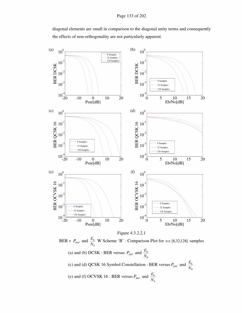
Page 133 of 202
diagonal elements are small in comparison to the diagonal unity terms and consequently
the effects of non-orthogonality are not particularly apparent.
-20 -10 0 10 2010
-4
10-3
10-2
10-1
100(a)
Psnr[dB]
BE
R D
CS
K8 Samples
32 Samples
128 Samples
0 5 10 15 2010
-4
10-3
10-2
10-1
100(b)
Eb/No[dB]
BE
R D
CS
K
8 Samples
32 Samples
128 Samples
-20 -10 0 10 2010
-4
10-3
10-2
10-1
100(c)
Psnr[dB]
BE
R Q
CS
K 1
6
8 Samples
32 Samples
128 Samples
0 5 10 15 2010
-4
10-3
10-2
10-1
100(d)
Eb/No[dB]
BE
R Q
CS
K 1
6
8 Samples
32 Samples
128 Samples
-20 -10 0 10 2010
-4
10-3
10-2
10-1
100(e)
Psnr[dB]
BE
R O
CV
SK
16
8 Samples
32 Samples
128 Samples
0 5 10 15 2010
-4
10-3
10-2
10-1
100(f)
Eb/No[dB]
BE
R O
CV
SK
16
8 Samples
32 Samples
128 Samples
Figure 4.3.2.2.1
BER v snrP and 0N
Eb W Scheme ‘B’ : Comparison Plot for ]128,32,8[∈n samples
(a) and (b) DCSK : BER versus snrP and 0N
Eb
(c) and (d) QCSK 16 Symbol Constellation : BER versus snrP and 0N
Eb
(e) and (f) OCVSK 16 : BER versus snrP and 0N
Eb

Page 134 of 202
-20 -10 0 10 2010
-4
10-3
10-2
10-1
100(a)
Psnr[dB]
BE
R
8 DCSK
32 DCSK
32 OCVSK 16
128 OCVSK 16
0 5 10 15 2010
-4
10-3
10-2
10-1
100(b)
Eb/No[dB]
BE
R
8 DCSK
32 DCSK
32 OCVSK 16
128 OCVSK 16
Figure 4.3.2.2.2
W Scheme ‘B’ Comparison of BER versus snrP and 0N
Eb for DCSK and OCVSK 16
Scheme showing a small divergence due to non-orthogonal reference signals.
4.3.2.3 W Matrix Case ‘C’
In this case the W matrix is given by
=
0000
0000
0000
1111
W (4.3.2.3.1)
=
1111
1111
1111
1111
WWT (4.3.2.3.2)
The above, as an example, is designed to illustrate a non banded W matrix. It represents
a set of signals which have all the columns of the U matrix the same and are completely
non-orthogonal, this is shown by the WWT
product in equation (4.3.2.3.2). Here the
span of BER, shown in figure (4.3.2.3.1) (e) and (f) for snrP , is infinite. This implies
that no information is transmitted at any value of snrP . The QCSK 16 examples of
figure (4.3.2.3.1) (c) and (d) use only the first two columns and rows of the W matrix.
In both cases, there is an improvement in the BER around the snrP values 0 dB to 10 dB.
This is clearly due, to the interaction of the signal noise distributions under the
estimation operations and does not represent any real information transmission.

Page 135 of 202
-20 -10 0 10 2010
-4
10-3
10-2
10-1
100(a)
Psnr[dB]
BE
R D
CS
K
8 Samples
32 Samples
128 Samples
0 5 10 15 2010
-4
10-3
10-2
10-1
100(b)
Eb/No[dB]
BE
R D
CS
K
8 Samples
32 Samples
128 Samples
-20 -10 0 10 2010
-4
10-3
10-2
10-1
100(c)
Psnr[dB]
BE
R Q
CS
K 1
6
8 Samples
32 Samples
128 Samples
0 5 10 15 2010
-4
10-3
10-2
10-1
100(d)
Eb/No[dB]
BE
R Q
CS
K 1
6
8 Samples
32 Samples
128 Samples
-20 -10 0 10 2010
-4
10-3
10-2
10-1
100(e)
Psnr[dB]
BE
R O
CV
SK
16
8 Samples
32 Samples
128 Samples
0 5 10 15 2010
-4
10-3
10-2
10-1
100(f)
Eb/No[dB]
BE
R O
CV
SK
16
8 Samples
32 Samples
128 Samples
Figure 4.3.2.3.1
BER v snrP and 0N
Eb W Scheme ‘C’ : Comparison Plot for ]128,32,8[∈n samples
(a) and (b) DCSK : BER versus snrP and 0N
Eb
(c) and (d) QCSK 16 Symbol Constellation : BER versus snrP and 0N
Eb
(e) and (f) OCVSK 16 : BER versus snrP and 0N
Eb

Page 136 of 202
-20 -10 0 10 2010
-4
10-3
10-2
10-1
100(a)
Psnr[dB]
BE
R
8 DCSK
32 DCSK
32 OCVSK 16
128 OCVSK 16
0 5 10 15 2010
-4
10-3
10-2
10-1
100(b)
Eb/No[dB]
BE
R
8 DCSK
32 DCSK
32 OCVSK 16
128 OCVSK 16
Figure 4.3.2.3.2
W Scheme ‘C’ Comparison of BER versus snrP and 0N
Eb for DCSK and OCVSK 16
Scheme showing the large divergence due to significantly non-orthogonal reference
signals
4.4 Summary
For the different system architectures presented in chapter 3, a set of simulation results
has been presented showing their various performance characteristics. The transmission
and BER simulations demonstrate the value of OCVSK methods utilizing orthogonal
signal sets over the extended M-ary type communications schemes.

Page 137 of 202
Chapter 5
Optimal Dimensionality
5.1 Introduction
In the previous chapters, it would seem that by constantly extending the dimension of
the suggested persistent type scheme in section (3.6.3), the transmission efficiency
could be endlessly increased. The only limiting factor would be the preamble of pre-
loading the orthogonal signal sets before useful transmission could take place. Another
limiting factor would be, a limit imposed by the method used to generate the orthogonal
sequence namely the Gram-Schmidt method. If the number of samples in each signal
sequence is n, then the number of orthogonal signals that can be generated is also n,
which if sufficiently large this is not really a limiting factor. However, experimentally,
when the case studies were being undertaken, benchmark transmission times weighed
against message transmission rates were empirically found to favour a value of around
seven or eight as the best choice of dimensionality m. Presented, is a mathematical
approach to determining why this might be the case. It considers the advantage over the
two dimensional M-ary type constellations, and the manner in which the surface layer
of hyperspheres; where the primary or most simple constellations of this method exist,
diminishes as a proportion of the total hypervolume as the dimension m increases.
Page 138 of 202
5.2 Volumetric Considerations
In QCSK, the constellations are represented on a unit circle which has an area of π . In
a hyperspace context this is a volume of order 2=m so π=)2(V . As we proceed from
dimension 2=m to dimension 3=m , the two dimensional volume occupies a zero
volume in the third dimensional space, but it can be integrated over the third orthogonal
dimension, to yield the familiar volumetric result π34)3( =V . The third dimension can
be considered as the space potentially occupied by the third ‘bit’ of our message, and if
we consider that the potential volume it can occupy lies within a hyperspherical shell
with radii of rr β± , where the β factor represents a banding of the noise variance i.e.
( )22rβσ = ; then we can derive an optimal value for dimensionality, compared with the
2=m dimensional value. This is described in section (5.3).
The volume of an m dimensional hypersphere of radius r is derived in appendix (D) and
can be expressed using the gamma )(zΓ function as
m
m rm
rV
m
⋅
+Γ
=
12
)(2π
(5.2.1)
Now consider a ratio mR of a hyperspherical shell of radii σ±r divided by the volume
of the hypercube containing the maximum radius that is )(2 σ+r
( )m
mmm
r
rVrVR
)(2
)()(
σ
σσ
+
−−+= (5.2.2)
where rβσ = and ]1,0(∈β
This can be considered as a measure of the efficiency of the volumetric concentration
near the surface of the m dimensional shell.

Page 139 of 202
5.3 Comparative Function
Before considering a more reasoned approach to determining the optimal dimension to
choose for the OCVSK scheme, it is worth considering how the distance between close
pairs of symbolic points in the constellations of the m dimensional space, compares with
the separation in the two dimensional M-ary type constellations. If all m dimensional
schemes are considered as simple; that is that each dimension has only a positive and a
negative value, then the distance between each successive symbolic point on a unit
hypersphere, with each point placed at an equal displacement along each axis illustrated
in figure (5.3.1) (a), is given by
12
2
=
dm (5.3.1)
yielding
md
2= (5.3.2)
And likewise, the separation of each symbolic value for the M-Ary scheme illustrated in
figure (5.3.1) (b) is given by
+
−=
−− 1
2
2
1
2
2sin
2cos1
mmd
ππ (5.3.3)
2
1
12cos12
−=
−md
π (5.3.4)
These functions for a continuously varying m are shown in figure (5.3.2) as a
comparative plot, and it clearly shows, that at 1=m and 2=m they are equal. This
corresponds to the BPSK and the Quadrature constellations respectively. At values of
2>m the OCVSK distance is always greater, which implies that the noise rejection is
always better. The value of m cannot exist for non integer values but the plot serves to
show the nature of the functions.
This is a good measure, but does not take into account the volumetric to available
surface effects described in [2][50], or any increase in computational loading. Firstly,
consider a comparison of the volumetric efficiency measure for an m dimensional
hyperspace mR and a similar measure of the 2=m dimensional hyperspace 2R .
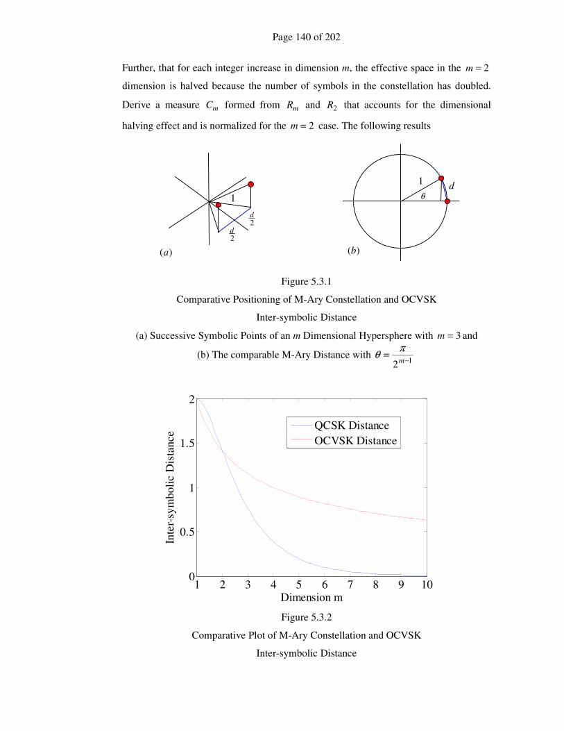
Page 140 of 202
1
θ d
)(b
1
2d
)(a
2d
Further, that for each integer increase in dimension m, the effective space in the 2=m
dimension is halved because the number of symbols in the constellation has doubled.
Derive a measure mC formed from mR and 2R that accounts for the dimensional
halving effect and is normalized for the 2=m case. The following results
Figure 5.3.1
Comparative Positioning of M-Ary Constellation and OCVSK
Inter-symbolic Distance
(a) Successive Symbolic Points of an m Dimensional Hypersphere with 3=m and
(b) The comparable M-Ary Distance with 12 −
=m
πθ
1 2 3 4 5 6 7 8 9 100
0.5
1
1.5
2
Dimension m
Inte
r-sy
mb
oli
c D
ista
nce
QCSK Distance
OCVSK Distance
Figure 5.3.2
Comparative Plot of M-Ary Constellation and OCVSK
Inter-symbolic Distance
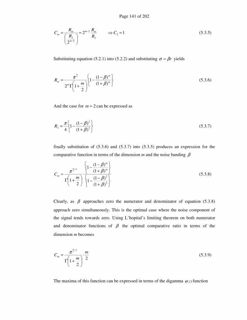
Page 141 of 202
2
2
2
2
2
2
R
R
R
RC mm
m
mm
−
−
=
= 12 =⇒C (5.3.5)
Substituting equation (5.2.1) into (5.2.2) and substituting rβσ = yields
+
−−
+Γ
=m
m
mm
mR
m
)1(
)1(1
212
2
β
βπ (5.3.6)
And the case for 2=m can be expressed as
+
−−=
2
2
2)1(
)1(1
4 β
βπR (5.3.7)
finally substitution of (5.3.6) and (5.3.7) into (5.3.5) produces an expression for the
comparative function in terms of the dimension m and the noise banding β
+
−−
+
−−
⋅
+Γ
=−
2
2
1
)1(
)1(1
)1(
)1(1
21
2
β
β
β
β
πm
m
mm
C
m
(5.3.8)
Clearly, as β approaches zero the numerator and denominator of equation (5.3.8)
approach zero simultaneously. This is the optimal case where the noise component of
the signal tends towards zero. Using L’hopital’s limiting theorem on both numerator
and denominator functions of β the optimal comparative ratio in terms of the
dimension m becomes
2
21
12 m
mC
m
m ⋅
+Γ
=−
π (5.3.9)
The maxima of this function can be expressed in terms of the digamma )(zϕ function

Page 142 of 202
m
m 2)ln(
21 =
−
+ πϕ (5.3.10)
This equation has no trivial solution, but the optimal solution occurs at a value of
2569.7=m a graph of equation (5.3.9) is shown in Figure (5.3.3). The derivation of this
result can be found in appendix (D.2)
0 5 7.2569 100
2
4
5.2778
6
Dimension m
Co
mp
arat
ive
Fu
nct
ion
Cm
Figure 5.3.3
Optimal Dimensional Value derived from Volumetric Considerations

Page 143 of 202
5.4 Dimensional Comparative Simulation
Consider a set of simulated Bit Error Rate (BER) ratios, between Orthogonal Chaotic
Vector Shift Keying (OCVSK) and M-ary versions of Quadrature Chaos Shift Keying
(QCSK), at various dimensions m between 3=m and 10=m . Now plot these against
snrP , the power of the signal to noise ratio, for sequences lengths of 128=n . This is
shown in figure (5.4.1).
-10 -5 0 510
-4
10-3
10-2
10-1
100
Psnr[dB]
Co
mpara
tive R
ati
o -
Bou
nd =
0.6
BER Ratio Dimensional Comparison
m=3
m=4
m=5
m=6
m=7
m=8
m=9
m=10
Figure 5.4.1
BER Ratio Dimensional Comparison
It clearly shows that as the dimension m moves through the 7=m value, the
improvement in BER Ratio stops and a subsequent increase in the dimension, increases
the BER Ratio at higher snrP values. It is also clear, that the benefit of using the higher
dimensional architectures is always an improvement over two dimensional quadrature
type schemes, as the fall off in the comparative function demonstrates. This simulation
is evaluated, with the estimate vector bounded between a magnitude of 0.4 and 1.6 for a
nominal value of 1.0. This is a wide band but clearly shows the dimensional effect. This
simulation run took several hours to complete, and finer bounding of the solutions
requires an exponential increase in computation time, to achieve reasonably smooth
curves. A listing of the Matlab code required to generate this plot is given in appendix
(D).
Page 144 of 202
5.5 Summary
In this chapter, a conjecture has been made as to why the empirical optimal dimension
of the OCVSK scheme is a value near seven. This has been approached by considering
a volume ratio of where the m-dimensional symbols exist in the communication space
and the maximal volume available for them to exist in. This has been derived as a
method of illustrating how the inter-symbolic distances vary with dimension. From this,
a comparative function between the m-dimensional scheme and an equivalent two
dimensional has been derived and shown to have a maximum at approximately seven.
In addition, it has been shown by simulations with varying noise conditions, that the
OCVSK scheme always has improved performance over any two dimensional M-ary
scheme and that the optimal value is approximately seven.

Page 145 of 202
Chapter 6
Conclusions
This thesis has presented a new method of improving the transmission efficiency of
chaotic communication schemes. Called Orthogonal Chaotic Vector Shift Keying, the
new method is based on orthogonal chaotic signal sequences. It has been shown that
under this multilevel digital communication scheme, significant improvements over
some existing methods, for example some typical M-ary type two-dimensional
quadrature schemes, have been achieved. Consequently, is has been demonstrated, that
the information transmitted per unit time is dependent on the dimensions adopted under
the new method.
A novel method of transmission and reception has been introduced whose only
overhead is an extended preamble time. The architectural requirements of this novel
scheme, have been investigated, using a number of different characterizable potential
signal structures. In addition, ways of improving the performance of these structural
schemes, by the careful choice of chaotic system and the conditional rejection of signal
sequences, has been demonstrated. The cyclic transmission efficiency is increased and
is scaleable with the dimension m, without any noise or time penalties.
The robustness and noise rejection properties of these multilevel schemes have been
demonstrated. Performance improvement comparisons, over typical M-ary type two
dimensional quadrature schemes, have been presented. The Bit Error Rates of the new
schemes have been shown to be equivalent to that of Differential Chaos Shift Keying.

Page 146 of 202
The nature of the methods employed in the schemes proposed has also potentially
increased the secure nature of the communications over a given channel.
Also in this thesis, a method has been demonstrated to characterize the nature of non-
linear processing elements of complex systems; and in turn, a simple modelling and
evaluation method, to determine the Bit Error Rates of these systems, has been derived
and the simulated results have been presented.
Investigation into the “optimal” dimensionality of the new method has shown that, the
optimal value for the scheme’s dimension is approximately seven. This is for the given
set of assumptions. For dimensions greater than seven, the improvement decreases, but
the new scheme always performs better than any two dimensional quadrature schemes.
The improvement decrease varies as a function of the relationship between the volume
of the communication space and the surface area of the hypersphere, where the
symbolic constellations lie. In addition, with higher dimensions, the computational
complexity increases approximately as the third order of the dimension.
Further suggested research work includes:
(1) Constellation Distribution on the Message Hypersphere
In the method presented in this thesis, the only type of constellation configuration
considered is the simple or bimodal one. That is that in each dimension there are two
symbols one with a positive value in the direction of the dimension axis, and the other,
with a negative value. As with QCSK and M-ary types of two-dimensional
constellations, this could be extended to higher orders, and the effect on transmission
efficiency and BER investigated. Work in this area could lead to finding an optimal
configuration for any given dimension m, and clarify the exact nature of optimality for
any configuration and dimension.
(2) Eigenvalue Symbol Information and Chaotic Orthogonal Signals

Page 147 of 202
For the method of Orthogonal Chaotic Vector Shift Keying, the orthogonalization of the
sampled matrices was achieved by using the Gram-Schmidt method. However, another
method of orthogonalization could be used which has some other properties usable in
future research. The method of Singular Valued Decomposition increases the
complexity of derivation but yields, for each set of sampled signals, a set of eigenvalues
associated with the matrix produced by the inner product of the sampled signal set.
These eigenvalues are very robust in a positional sense, in the presence of high levels of
noise and could be used as message symbol sets. The problem then becomes reversed in
the sense that for a given set of eigenvalues, representing a complex multilevel message,
the problem of how to directly generate a set of orthogonal chaotic signals needs to be
researched.
(3) Hyperchaotic Generating Systems
The pseudo cyclic behaviour of the Lorenz system, chosen in the thesis, has two distinct
disadvantages. Firstly, the cyclical signals although not constant, are detectable and
secondly, the same cyclical nature can potentially result in a high number of signal
sequence rejections, due to insufficient independence of the columns of the sampled
matrix. These two problems could be overcome by employing hyperchaotic systems.
The research would then be aimed at a decision process for the most appropriate system.
Page 148 of 202
References
[1] Digital Communications Systems
P. Z. Peebles Jr.
Prentice Hall International Inc., New Jersey, USA, 1987
[2] Telecommunications Engineering
J. Dunlop and D. Smith
Van Nostrand Reinhold (UK) Co. Ltd., Berkshire, England, 1984
[3] Information Transmission Modulation and Noise 3rd
Edition
M. Schwartz
McGraw-Hill, Maidenhead, 1980
[4] Synchronization in Chaotic Systems
L. K. Pecora and T. L. Carroll
Phys. Rev. Lett. , Volume 64, Issue 8, 1990, Page(s): 821-824
[5] Driving Systems with Chaotic Signals
L. K. Pecora and T. L. Carroll
Phys. Rev. A, Volume 44, Number 4, 1991, Page(s): 2374-2384
[6] Circuit Implementation of Synchronized Chaos with Applications to
Communications
K. M. Cuomo and A. V. Oppenheim
Phys. Rev. Lett. , Volume 71, Issue 1, 1993, Page(s): 65-68
Page 149 of 202
[7] Synchronizing Hyperchaotic Volume-Preserving Maps and Circuits
T. L. Carroll and L. M. Pecora
IEEE Transactions on Circuits and Systems I
Fundamental Theory and Applications, Vol. 45, Issue 6, 1998 Page(s): 656-659
[8] Using Cyclostationary Properties of Chaotic Signals for Communications
T. Carroll
IEEE Transactions on Circuits and Systems I
Fundamental Theory and Applications, Vol. 49, Issue 3, 2002 Page(s): 357-362
[9] Implementation of Bidirectional Chaotic Communications Systems Based on
Lorenz Circuits
S. Tsay, C. Huang, D. Qiu and W. Chen
Chaos Solitons and Fractals, 20, 2004, Page(s): 567-579
[10] Basic Principles of Direct Chaotic Communications Systems
A. Dmitriev, M Hasler, A. Panas and K. Zakharchenko
Nonlinear Phenomena in Complex Systems, Vol. 4, Issue 1, 2002 Page(s): 1-14
[11] Design of Noncoherent Receiver for Analog Spread Spectrum Communication
Based on Chaotic Masking
K. Murali, H. Leung and H. 3
IEEE Transactions on Circuits and Systems I
Fundamental Theory and Applications, Vol. 50, Issue 10, 2003 Page(s): 432-441
[12] The Role of Synchronization in Digital Communications Using Chaos – Part II:
Chaotic Modulation and Chaotic Synchronization
G. Kolumbán, M. P. Kennedy and L. O. Chua
IEEE Transactions on Circuits and Systems I
Fundamental Theory and Applications, Vol. 45, Issue 11, 1998 Page(s): 1129-
1140

Page 150 of 202
[13] Performance Analysis of Correlation-Based Communication Schemes Utilizing
Chaos
M. Sushchik, L. S. Tsimring and A. R. Volkovskii
IEEE Transactions on Circuits and Systems I
Fundamental Theory and Applications, Vol. 47, Issue 12, 2000 Page(s): 1684-
1691
[14] On Some Recent Developments of Noise Cleaning Algorithms for Chaotic
Signals
Z. J. Jako, G. Kolumbán and H. Dedieu
IEEE Transactions on Circuits and Systems I
Fundamental Theory and Applications, Vol. 47, Issue 9, 2000 Page(s): 1403-
1406
[15] Noise Performance of Chaotic Communication Systems
A. Abel, W. Schwarz and M. Gotz
IEEE Transactions on Circuits and Systems I
Fundamental Theory and Applications, Vol. 47, Issue 12, 2000 Page(s): 1726-
1732
[16] Performance of Differential Chaos-Shift-Keying Digital Communication Systems
over a Multipath Fading Channel with Delay Spread
Y. Xia, C. K. Tse and F. Lau
IEEE Transactions on Circuits and Systems II
Express Briefs, Vol. 51, Issue 12, 2004 Page(s): 680-684
[17] Performance Evaluation of FM-DCSK Modulation in Multipath Environments
M. P. Kennedy, G. Kolumban, G. Kis and Z. Jako
IEEE Transactions on Circuits and Systems I
Fundamental Theory and Applications, Vol. 47, Issue 12, 2000 Page(s): 1702-
1711
Page 151 of 202
[18] Optimal Detection of Differential Chaos Shift Keying
T. Schimming and M. Hasler
IEEE Transactions on Circuits and Systems I
Fundamental Theory and Applications, Vol. 47, Issue 12, 2000 Page(s): 1712-
1719
[19] Essence and Advantages of FM-DCSK Technique versus Conventional Spreading
Spectrum Communication Method
L. Ye, G. Chen and L. Wang
http://www.paper.edu
[20] Analysis and CMOS Implementation of a Chaos-Based Communication System
S. Mandal and S. Banerjee
IEEE Transactions on Circuits and Systems I
Regular Papers, Vol. 51, Issue 9, 2004 Page(s): 1708-1722
[21] Applications of Symbolic Dynamics to Differential Chaos Shift Keying
G. M. Maggio and Z. Galias
IEEE Transactions on Circuits and Systems I
Fundamental Theory and Applications, Vol. 49, Issue 12, 2002 Page(s): 1729-
1735
[22] Enhanced Differential Chaos Shift Keying Using Symbolic Dynamics
G. Maggio and Z. Galias
University of Mining and Metallurgy, Krakow, Poland
[23] A Chaos Based Spread Spectrum Communication System
S. Mandal and S. Banerjee
Chaos Solitons and Fractals, 20, 2004, Page(s): 567-579
Page 152 of 202
[24] Quadrature Chaos-Shift Keying
Z. Galias and G. M. Maggio
Institute of Non-linear Science, University of California; Proposal for
IEEE Transactions on Circuits and Systems I
Fundamental Theory and Applications, Vol. 48, Issue 12, 2001 Page(s): 1510-
1519
[25] An Observer-Based Approach for Input-Independent Global Chaos
Synchronization of Discrete-Time Switched Systems
G. Millerioux and J. Daafouz
IEEE Transactions on Circuits and Systems I
Fundamental Theory and Applications, Vol. 50, Issue 10, 2003 Page(s): 1270-
1279
[26] Synchronizing Hyperchaotic Systems by Observer Design
G. Grasse and S. Mascolo
IEEE Transactions on Circuits and Systems II
Analogue and Digital Signal Processing, Vol. 46, Issue 4, 1999 Page(s): 478-483
[27] Observer Based Synchronization and Input Recovery for a Class of Nonlinear
Chaotic Models
E. Cherrier, M. Boutayeb and J. Ragot
44th
Conference on Decision and Control, March 2005
[28] Synchronization of Chaotic Systems via Nonlinear Control
L. Huang, R. Feng and M. Fao
Physics Letters A, 320, 2004, Page(s): 271-275
[29] Extracting Messages Masked by Chaos
P. Gabriel and H. A. Cerdeira
Phys. Rev. Lett. , Volume 74, Issue 11, 1995, Page(s): 1970-1973
Page 153 of 202
[30] Partial Identification of Lorenz System and its Application to Key Space
Reduction of Chaotic Cryptosystems
E. Solak
IEEE Transactions on Circuits and Systems II
Express Briefs, Vol. 51, Issue 10, 2004 Page(s): 557-560
[31] Breaking Two Secure Communication Schemes Based on Chaotic Masking
G. Alvarez, F. Montoya, M. Romera and G. Pastor
IEEE Transactions on Circuits and Systems II
Express Briefs, Vol. 51, Issue 10, 2004 Page(s): 505-506
[32] Analysis of Some Recently proposed Chaos-Based Encryption Algorithms
G. Jakimoski and L. Kocarev
Physics Letters A, 291, 2001, Page(s): 381-384
[33] On Optimal Detection of Noncoherent Chaos Shift Keying Signals in a Noisy
Environment
F. Lau and C. Tse
International Journal of Bifurcation and Chaos, Vol. 13, Issue 6, 2003, Page(s):
1587-1597
[34] A New Chaotic Communications Scheme
Z. Li, K. Li, C. Wen and Y. C. Soh
IEEE Transactions on Communications, Vol. 51, Issue 8, 2003 Page(s): 1306-
1312
[35] Additive Mixing Modulation for Public Key Encryption Based on Distributed
Dynamics
R. Tenny and L. S. Tsimring
IEEE Transactions on Circuits and Systems I
Regular Papers, Vol. 52, Issue 3, 2003 Page(s): 672-679
Page 154 of 202
[36] New Approach to Chaotic Encryption
E. Alvarez, A. Fernandez, P. Garcia, J. Jimenez and A. Marcano
Physics Letters A, 263, 1999, Page(s): 373-375
[37] Permutation Based DCSK and Multiple Access DCSK Systems
F. Lau, K. Cheong and C. Tse
IEEE Transactions on Circuits and Systems I
Fundamental Theory and Applications, Vol. 50, Issue 6, 2003 Page(s): 733-742
[38] Exact Calculation of Bit Error Rates in Communication Systems with Chaotic
Modulation
A. J. Lawrance and G. Ohama
IEEE Transactions on Circuits and Systems I
Fundamental Theory and Applications, Vol. 50, Issue 11, 2003 Page(s): 1391-
1400
[39] Noise Performance of Chaotic Communication Systems
A. Abel, W. Schwarz and M. Gotz
IEEE Transactions on Circuits and Systems I
Fundamental Theory and Applications, Vol. 47, Issue 12, 2003 Page(s): 1726-
1732
[40] On the Threshold Effect in the Estimation of Chaotic Sequences
I. Hen and N. Merhav
IEEE Transactions on Information Theory, Vol. 50, Issue 11, 2003 Page(s): 2894-
2904
[41] Theoretical Noise Performance of Correlator-Based Chaotic Communications
Schemes
G. Kolumbán
IEEE Transactions on Circuits and Systems I
Fundamental Theory and Applications, Vol. 47, Issue 12, 2003 Page(s): 1692-
1701

Page 155 of 202
[42] Applications of Stochastic Calculus and Ergodic Theory in Chaotic
Communication Theory
C. Chen and K. Yao
Nonlinear Analysis, 47, 2001, Page(s): 5775-5784
[43] Optimal and Suboptimal Chaos Receivers
M. Hasler and T. Schimming
Invited Paper
[44] Towards Full Characterization of Continuous Systems in Terms of Periodic Orbits
Z. Galias
Department of Electrical Engineering, University of Science and Technology,
Krakow, Poland
[45] Deterministic Nonperiodic Flow
E. N. Lorenz
Journal of the Atmospheric Sciences, Vol. 20, Issue 2 Page(s): 130-141, 1963
[46] Chaos in Dynamical Systems (2nd
Edition)
E. Ott
Cambridge University Press, 2002
[47] Chaotic Behaviour of Multidimensional Difference Equations
Kaplan and J. A. Yorke
Lecture Notes in Mathematics, 730, Springer, Berlin, 1979, Page(s): 204
[48] Digital Signal Processing: A Practical Approach
E. C. Ifeachor and B. W. Jervis
Addison Wesley Publishers Ltd., Harlow, England, 1998
[49] The Fast Fourier Transform
O. Brigham
Prentice-Hall, London and New Jersey, 1974
Page 156 of 202
[50] A Mathematical Theory of Communication
C. Shannon
Bell Systems Technical Journal, Issue 27, Page(s): 379-423, 1948
[51] Multivariable System Theory and Design
R. V. Patel and N. Munro
Pergamon Press, Oxford, England, 1982
[52] Digital Control
G. F. Franklin and J. D. Powell
Addison Wesley, Philippines, 1980
[53] Modern Control Systems: A Manual of Design Methods
J. Borrie
Prentice Hall, Hemel Hempstead, England, 1986
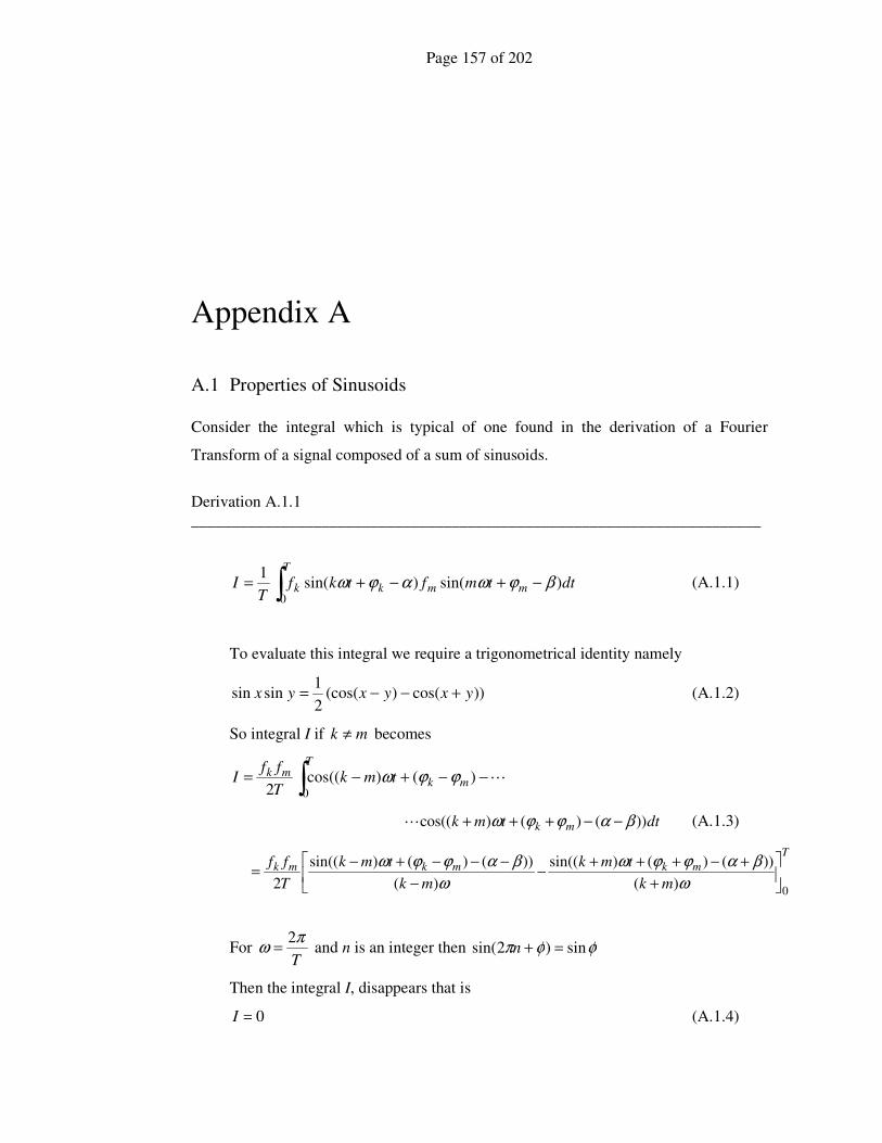
Page 157 of 202
Appendix A
A.1 Properties of Sinusoids
Consider the integral which is typical of one found in the derivation of a Fourier
Transform of a signal composed of a sum of sinusoids.
Derivation A.1.1
______________________________________________________________________
dttmftkfT
I mmk
T
k )sin()sin(1
0
βϕωαϕω −+−+= ∫ (A.1.1)
To evaluate this integral we require a trigonometrical identity namely
))cos()(cos(2
1sinsin yxyxyx +−−= (A.1.2)
So integral I if mk ≠ becomes
L−−+−= ∫ )()cos((2 0
m
T
kmk tmk
T
ffI ϕϕω
dttmk mk ))()()cos(( βαϕϕω −−+++L (A.1.3)
T
mkmkmk
mk
tmk
mk
tmk
T
ff
0)(
))()()sin((
)(
))()()sin((
2
+
+−+++−
−
−−−+−=
ω
βαϕϕω
ω
βαϕϕω
For T
πω
2= and n is an integer then φφπ sin)2sin( =+n
Then the integral I, disappears that is
0=I (A.1.4)

Page 158 of 202
Likewise integral I, if mk = becomes
∫ +−+−−=T
kk dttkT
fI
0
2
))(22cos()cos(2
βαϕωαβ
Tkk
k
tkt
T
f
0
2
2
))(22sin()cos(
2
+−+−−=
ω
βαϕωαβ
)cos(2
2
αβ −= kf (A.1.5)
______________________________________________________________________
A.2 Fourier Transform Pairs
The Fourier Transform pair is given by
Result A.2.1
______________________________________________________________________
∫
∫∞
∞−
∞
∞−
−
=
=
ωωπ
ω
ω
ω
dejHth
dtethjH
tj
tj
)(2
1)(
)()(
(A.2.1)
______________________________________________________________________
Also the following important result will be required
Result A.2.1
______________________________________________________________________
)(sin
ωπδω
ω=
∞→
TLimT
(A.2.2)
______________________________________________________________________
This property comes from a nascent definition of the Dirac delta function which is given
by
=
aa
ω
πωωδ sin
1)( (A.2.3)
Now the actual delta function is defined by any nascent function as
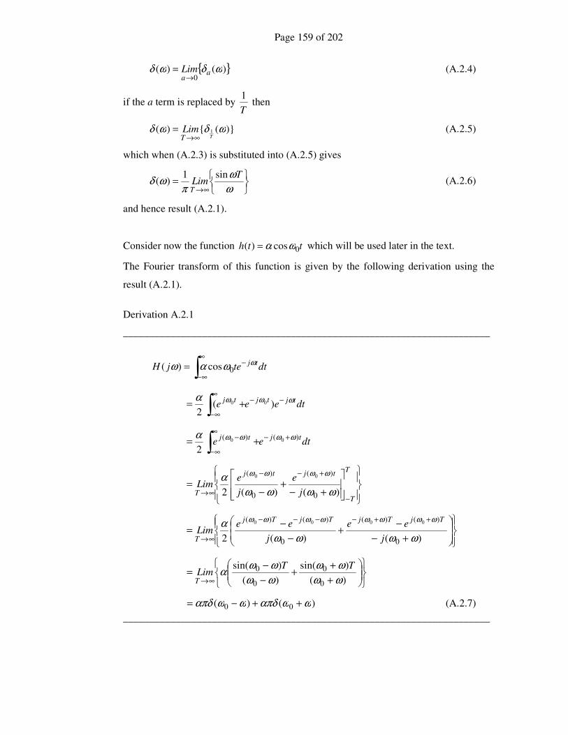
Page 159 of 202
{ })()(0
ωδωδ aaLim
→= (A.2.4)
if the a term is replaced by T
1 then
)}({)( 1 ωδωδTT
Lim∞→
= (A.2.5)
which when (A.2.3) is substituted into (A.2.5) gives
=∞→ ω
ω
πωδ
TLimT
sin1)( (A.2.6)
and hence result (A.2.1).
Consider now the function tth 0cos)( ωα= which will be used later in the text.
The Fourier transform of this function is given by the following derivation using the
result (A.2.1).
Derivation A.2.1
______________________________________________________________________
∫∞
∞−
−= dttejHtjωωαω 0cos)(
dteeetjtjtj ωωωα −−
∞
∞−∫ += )(2
00
dteetjtj )()( 00
2
ωωωωα +−∞
∞−
−∫ +=
+−+
−=
−
+−−
∞→
T
T
tjtj
T j
e
j
eLim
)()(2 0
)(
0
)( 00
ωωωω
α ωωωω
+−
−+
−
−=
++−−−−
∞→ )()(2 0
)()(
0
)()( 0000
ωωωω
α ωωωωωωωω
j
ee
j
eeLim
TjTjTjTj
T
+
++
−
−=
∞→ )(
)sin(
)(
)sin(
0
0
0
0
ωω
ωω
ωω
ωωα
TTLim
T
)()( 00 ωωαπδωωαπδ ++−= (A.2.7)
______________________________________________________________________

Page 160 of 202
0ω 0ω−
Real Imaginary
This result can be represented on two diagrams showing the real and imaginary parts of
the derived phasor delta functions.
Figure A.2.1
Resultant Phasors for tth 0cos)( ωα=
Now for completeness show that the inverse transform recreates the original signal
when applied to the result of derivation (A.2.1)
Derivation A.2.2
______________________________________________________________________
( )∫∞
∞−
++−= ωωωαπδωωαπδπ
ωdeth
tj)()(2
1)( 00
( )tjtjee 00
2
ωωα −+=
t0cosωα= (A.2.8)
______________________________________________________________________
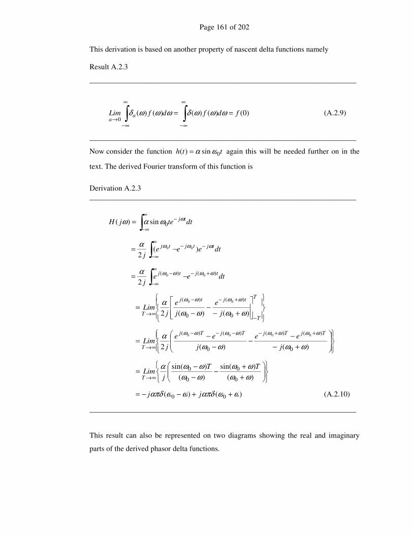
Page 161 of 202
This derivation is based on another property of nascent delta functions namely
Result A.2.3
______________________________________________________________________
)0()()()()(0
fdfdfLim aa
== ∫∫∞
∞−
∞
∞−→
ωωωδωωωδ (A.2.9)
______________________________________________________________________
Now consider the function tth 0sin)( ωα= again this will be needed further on in the
text. The derived Fourier transform of this function is
Derivation A.2.3
______________________________________________________________________
∫∞
∞−
−= dttejHtjωωαω 0sin)(
dteeej
tjtjtj ωωωα −−∞
∞−∫ −= )(2
00
dteej
tjtj )()( 00
2
ωωωωα +−∞
∞−
−∫ −=
+−−
−=
−
+−−
∞→
T
T
tjtj
T j
e
j
e
jLim
)()(2 0
)(
0
)( 00
ωωωω
α ωωωω
+−
−−
−
−=
++−−−−
∞→ )()(2 0
)()(
0
)()( 0000
ωωωω
α ωωωωωωωω
j
ee
j
ee
jLim
TjTjTjTj
T
+
+−
−
−=
∞→ )(
)sin(
)(
)sin(
0
0
0
0
ωω
ωω
ωω
ωωα TT
jLim
T
)()( 00 ωωαπδωωαπδ ++−−= jj (A.2.10)
______________________________________________________________________
This result can also be represented on two diagrams showing the real and imaginary
parts of the derived phasor delta functions.

Page 162 of 202
0ω
0ω−
Real Imaginary
Figure A.2.2
Resultant Phasors for tth 0sin)( ωα=
Now also for completeness show that the inverse transform recreates the original signal
when applied to the derivation (A.2.3)
Derivation A.2.4
______________________________________________________________________
( )∫∞
∞−
++−−= ωωωαπδωωαπδπ
ωdejjth
tj)()(2
1)( 00
( )
( )tjtj
tjtj
eej
eej
00
00
2
2
ωω
ωω
α
α
−
−
−=
+−=
t0sin ωα= (A.2.11)
______________________________________________________________________
Now consider a case required for analysing real signals consisting of a sinusoidal signal
shifted by some arbitrary phase )sin()( 0 ϕωα += tth
Then the Fourier transform of this function is derived as follows
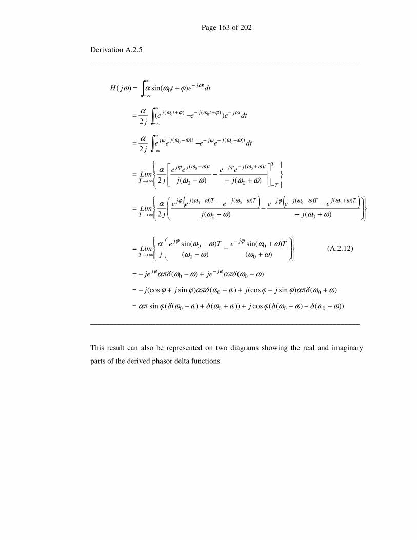
Page 163 of 202
Derivation A.2.5
______________________________________________________________________
∫∞
∞−
−+= dtetjHtjωϕωαω )sin()( 0
dteeej
tjtjtj ωϕωϕωα −+−∞
∞−
+∫ −= )(2
)()( 00
dteeeej
tjjtjj )()( 00
2
ωωϕωωϕα +−−∞
∞−
−∫ −=
+−−
−=
−
+−−−
∞→
T
T
tjjtjj
T j
ee
j
ee
jLim
)()(2 0
)(
0
)( 00
ωωωω
α ωωϕωωϕ
( ) ( )
+−
−−
−
−=
++−−−−−
∞→ )()(2 0
)()(
0
)()( 0000
ωωωω
α ωωωωϕωωωωϕ
j
eee
j
eee
jLim
TjTjjTjTjj
T
+
+−
−
−=
−
∞→ )(
)sin(
)(
)sin(
0
0
0
0
ωω
ωω
ωω
ωωα ϕϕTeTe
jLim
jj
T (A.2.12)
)()( 00 ωωαπδωωαπδ ϕϕ ++−−= − jj jeje
)()sin(cos)()sin(cos 00 ωωαπδϕϕωωαπδϕϕ +−+−+−= jjjj
))()((cos))()((sin 0000 ωωδωωδϕωωδωωδϕαπ −−++++−= j
______________________________________________________________________
This result can also be represented on two diagrams showing the real and imaginary
parts of the derived phasor delta functions.

Page 164 of 202
0ω
0ω−
Real Imaginary
0ω− 0ω
Figure A.2.3
Resultant Phasors for )sin()( 0 ϕωα += tth
MATLAB Function A.2.1– OrthogonalSignal
______________________________________________________________________
function y=OrthogonalSignal(x,n)
c=sqrt(-1);
z=fft(x);
for i=1:n/2
z(i) = -c*z(i);
end;
for i=1+n/2:n
z(i) = c*z(i);
end;
y=ifft(z);
y=real(y);
______________________________________________________________________

Page 165 of 202
A.3 Lyapunov Exponent Calculation Listings
MATLAB Function A.3.1– CalcLyapunov
______________________________________________________________________
[T,H,X]=Lyapunov(3,@Lorenz_Variational,@ode45,0,0.01,200,[1 0 0],100);
figure(1);
plot(T,H);
title('Dynamics of Lyapunov exponents');
xlabel('Time'); ylabel('h - Lyapunov exponents');
figure(2);
plot3(X(:,1),X(:,2),X(:,3));
title('State Space Plot');
______________________________________________________________________
MATLAB Function A.3.2 – Lyapunov
______________________________________________________________________ function [T,H,X]=Lyapunov(n,SystemHandle,IntegratorHandle,
tStart,tStep,tEnd,xStart,OutputCount);
% Values of parameters
SIGMA = 10;
R = 28;
BETA = 8/3;
% Memory allocation
LogSum = zeros(1,n);
h = zeros(1,n);
% Initial values
N = n*(n + 1);
X = xStart(:)';
% Form integration vector
intVec(1:N) = [X' eye(n,n)];
% Main loop
nSteps = round((tEnd - tStart)/tStep);
t = tStart;
for Iteration = 1:nSteps
% Solution of extended ODE system
[TVec,Result] = feval(IntegratorHandle,SystemHandle,[t t +
tStep],intVec);
% Form next iteration Y matrix
intVec = Result(size(Result,1),:);
% Nonlinear state
x = intVec(1:n);
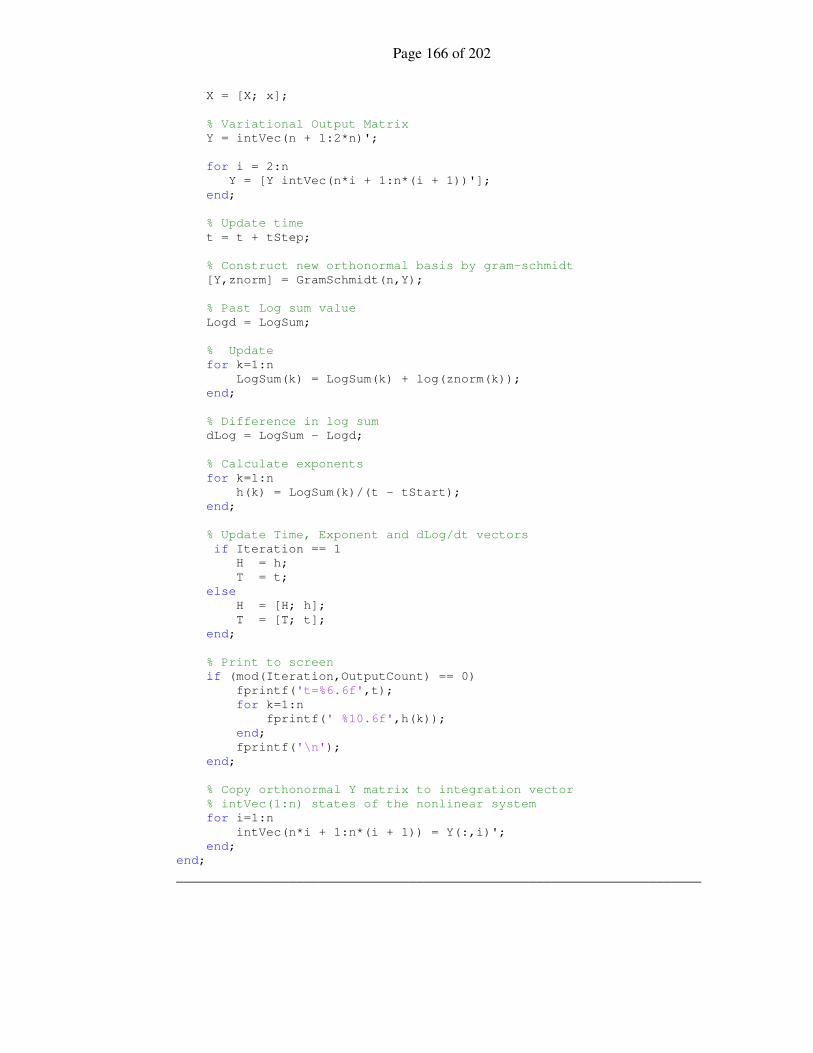
Page 166 of 202
X = [X; x];
% Variational Output Matrix
Y = intVec(n + 1:2*n)';
for i = 2:n
Y = [Y intVec(n*i + 1:n*(i + 1))'];
end;
% Update time
t = t + tStep;
% Construct new orthonormal basis by gram-schmidt
[Y,znorm] = GramSchmidt(n,Y);
% Past Log sum value
Logd = LogSum;
% Update
for k=1:n
LogSum(k) = LogSum(k) + log(znorm(k));
end;
% Difference in log sum
dLog = LogSum - Logd;
% Calculate exponents
for k=1:n
h(k) = LogSum(k)/(t - tStart);
end;
% Update Time, Exponent and dLog/dt vectors
if Iteration == 1
H = h;
T = t;
else
H = [H; h];
T = [T; t];
end;
% Print to screen
if (mod(Iteration,OutputCount) == 0)
fprintf('t=%6.6f',t);
for k=1:n
fprintf(' %10.6f',h(k));
end;
fprintf('\n');
end;
% Copy orthonormal Y matrix to integration vector
% intVec(1:n) states of the nonlinear system
for i=1:n
intVec(n*i + 1:n*(i + 1)) = Y(:,i)';
end;
end;
______________________________________________________________________

Page 167 of 202
MATLAB Function A.3.3 – Lorenz_Variational
______________________________________________________________________ function f=Lorenz_Variational(t,X)
% Values of parameters
Sigma = 10;
R = 28;
Beta = 8/3;
x=X(1);
y=X(2);
z=X(3);
Y= [X(4), X(7), X(10);
X(5), X(8), X(11);
X(6), X(9), X(12)];
f=zeros(12,1);
%Lorenz equation
f(1) = Sigma*(y - x);
f(2) = -x*z + R*x - y;
f(3) = x*y - Beta*z;
%Linearized system
Jacobian = [-Sigma, Sigma, 0;
R – z, -1, -x;
y, x, -Beta];
%Variational equation
f(4:12)=Jacobian*Y;
_______________________________________________________

Page 168 of 202
11, vx
2x
1u
2u
2v
111
12
,
,v
vv
vx
Appendix B
B.1 Gram-Schmidt Method
The Gram-Schmidt method is used to orthonormalize a set of m arbitrary n dimensional
vectors ],1[ miRn
i ∈∈u where nm ≤ that span an m dimensional subspace in an n
space.
Result B.1
______________________________________________________________________
Consider a set of m vectors of dimension n that span a real subspace of dimension
m : ],1[ miRni ∈∈x . A set of vectors ],1[ miRn
i ∈∈u can be generated from
ix which form an orthonormal basis and spans the same m dimensional subspace.
Figure B.1.1
First Stage of Gram-Schmidt Method

Page 169 of 202
The algorithm follows as
Choose the first vector
11 xv = (B.1.1)
and determine its magnitude
11 v=α (B.1.2)
then the first member of the orthonormal set is given by
1
11
α
vu = (B.1.3)
Now choose the second vector from the set 2x and remove the component that
corresponds to the direction of 1x as illustrated in figure (B.1.1) giving
111
1222
,
,v
vv
vxxv −= (B.1.4)
and as before
22 v=α (B.1.5)
then the next member of the orthonormal set is given by
2
22
α
vu = (B.1.6)
For the next member of the set all the components in the directions of the
previously calculated set ]1,1[ −∈∀ kiiv must be removed yielding the following
algorithm.
∑−
=
−=
1
1,
,k
i
iii
ikkk v
vv
vxxv
kk v=α
k
kk
α
vu = (B.1.7)
This algorithm can be made more numerically stable by, iteratively calculating the
summing term and using the previous orthonormal basis set members, instead of
the original set members. This is most easily illustrated in the following algorithm
______________________________________________________________________

Page 170 of 202
Algorithm B.1
______________________________________________________________________
for mk :1=
kk xv =
for 1:1 −= ki
iikkk uuvvv ,−=
end
kk v=α
k
kk
α
vu =
end
______________________________________________________________________

Page 171 of 202
Appendix C C.1 Transmission Simulation MATLAB Function Listings
The following functions are used to generate graphs for section (4.2) of this thesis
simulating the transmission schemes over a noisy channel.
MATLAB Function C.1.1 – SystemU
This function simulates transmission over a noisy communication channel in either the
‘U’ scheme or the ‘X’ scheme described in chapter 3.
______________________________________________________________________ % Usage: % % n Number of samples per signal vector : n % m Dimension of Scheme : m % Fig First figure number : 1 % Psnr Signal to noise power ratio : 1.0 % Sigma Noise standard deviation : 1.0 % Runs Number of simulation runs : 10 % Scheme Type of Scheme : 'X' % % [Result,MessageT,Bt,Be]=SystemU(n,m,Fig,Psnr,Sigma,Runs,Scheme)
function [Result,MessageT]=SystemU(n,m,Fig,Psnr,Sigma,Runs,Scheme)
Plot=1;
% Initialize System [T,x,t,MessMax,EncodingMap]=Initialize(n,m);
P=Sigma*sqrt(n*Psnr)*eye(m);
MessageT=zeros(Runs+1,1); MessageR=zeros(Runs+1,1); MessageError=zeros(Runs+1,1); Mt=zeros(Runs+1,m); Mr=zeros(Runs+1,m);

Page 172 of 202
Me=zeros(Runs+1,m);
Qt =zeros(n,m); St =zeros(n,m); Zt =zeros(n,m);
Ct=zeros(m,m);
Count=1; Error=1; Result=0;
% To simulate transmission delay % run receive code first while Runs
% Calculate Noise Matrices Nq=Sigma*randn(n,m); Ns=Sigma*randn(n,m);
% Decode m Messages if Scheme == 'U' Qr=Qt+Nq; Sr=St+Ns;
if Plot figure(Fig+4); plot(Qr); str=sprintf('Received Q Matrix Balanced Orthogonal
References'); title(str); xlabel('Samples'); nstr=sprintf('%s.fig',str); saveas(gcf,nstr); nstr=sprintf('%s.bmp',str); saveas(gcf,nstr); figure(Fig+5); plot(Sr); str=sprintf('Received S Matrix Encoded Messages'); title(str); xlabel('Samples'); nstr=sprintf('%s.fig',str); saveas(gcf,nstr); nstr=sprintf('%s.bmp',str); saveas(gcf,nstr); end; else Zr=Zt+Nq; Sr=St+Ns; [U,Betat]=GramSchmidt(m,Zr); Qr=U*P;
if Plot figure(Fig+4); plot(Zr); str=sprintf('Received Z Matrix Balanced References'); title(str); xlabel('Samples'); nstr=sprintf('%s.fig',str); saveas(gcf,nstr);

Page 173 of 202
nstr=sprintf('%s.bmp',str); saveas(gcf,nstr); figure(Fig+5); plot(Sr); str=sprintf('Received S Matrix Encoded Messages'); title(str); xlabel('Samples'); nstr=sprintf('%s.fig',str); saveas(gcf,nstr); nstr=sprintf('%s.bmp',str); saveas(gcf,nstr); end; end;
Cr=inv(Qr'*Qr)*Qr'*Sr;
C=Cr; for i=1:m for j=1:m if C(i,j) < 0.0 C(i,j)=-1/sqrt(m); else C(i,j)=1/sqrt(m); end; end; end; for k=1:m for kk=1:2^m if C(:,k)==(EncodingMap(:,kk)/sqrt(m)) Mr(Count,k)=kk-1; break; end; end; end;
MessageR(Count)=0; j=1; for i=1:m MessageR(Count)=MessageR(Count)+Mr(Count,i)*2^m^(m-j); j=j+1; end;
% Error calculation if Count > 1 MessageError(Count)=MessageT(Count-1)-MessageR(Count); Me(Count,:)=Mt(Count-1,:)-Mr(Count,:); end;
if MessageError(Count) if Error == 1 Result=[Count MessageError(Count)/MessMax Betat']; else Result=[Result;[Count MessageError(Count)/MessMax Betat']]; end; Error=Error+1; end;
if Plot figure(Fig+6); stairs(MessageT);
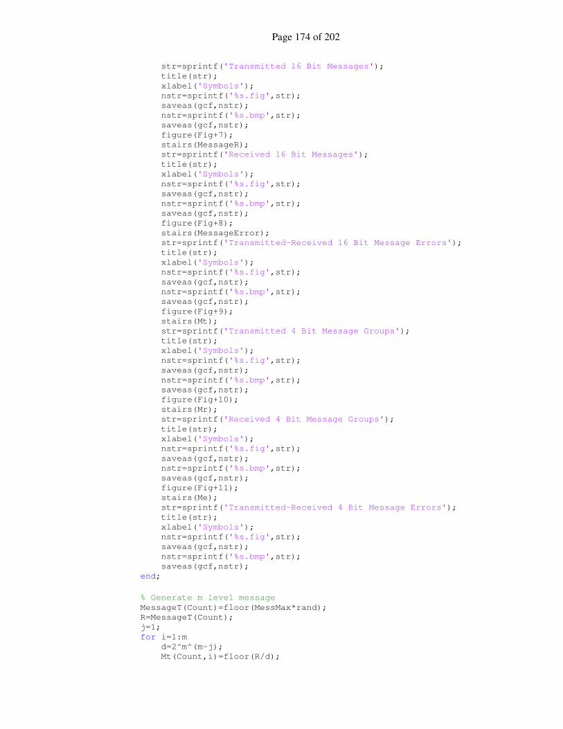
Page 174 of 202
str=sprintf('Transmitted 16 Bit Messages'); title(str); xlabel('Symbols'); nstr=sprintf('%s.fig',str); saveas(gcf,nstr); nstr=sprintf('%s.bmp',str); saveas(gcf,nstr); figure(Fig+7); stairs(MessageR); str=sprintf('Received 16 Bit Messages'); title(str); xlabel('Symbols'); nstr=sprintf('%s.fig',str); saveas(gcf,nstr); nstr=sprintf('%s.bmp',str); saveas(gcf,nstr); figure(Fig+8); stairs(MessageError); str=sprintf('Transmitted-Received 16 Bit Message Errors'); title(str); xlabel('Symbols'); nstr=sprintf('%s.fig',str); saveas(gcf,nstr); nstr=sprintf('%s.bmp',str); saveas(gcf,nstr); figure(Fig+9); stairs(Mt); str=sprintf('Transmitted 4 Bit Message Groups'); title(str); xlabel('Symbols'); nstr=sprintf('%s.fig',str); saveas(gcf,nstr); nstr=sprintf('%s.bmp',str); saveas(gcf,nstr); figure(Fig+10); stairs(Mr); str=sprintf('Received 4 Bit Message Groups'); title(str); xlabel('Symbols'); nstr=sprintf('%s.fig',str); saveas(gcf,nstr); nstr=sprintf('%s.bmp',str); saveas(gcf,nstr); figure(Fig+11); stairs(Me); str=sprintf('Transmitted-Received 4 Bit Message Errors'); title(str); xlabel('Symbols'); nstr=sprintf('%s.fig',str); saveas(gcf,nstr); nstr=sprintf('%s.bmp',str); saveas(gcf,nstr); end;
% Generate m level message MessageT(Count)=floor(MessMax*rand); R=MessageT(Count); j=1; for i=1:m d=2^m^(m-j); Mt(Count,i)=floor(R/d);
Page 175 of 202
R=R-Mt(Count,i)*d; j=j+1; end;
% Encode m messages Ct=zeros(m,m); for i=1:m Ct(:,i) = EncodingMap(:,Mt(Count,i)+1)/sqrt(m); end;
% Create Reference [Xt,x]=Chaos(n,m,x,T); if Plot figure(Fig); plot(Xt); str=sprintf('X Matrix Chaotic Sequences'); title(str); xlabel('Samples'); nstr=sprintf('%s.fig',str); saveas(gcf,nstr); nstr=sprintf('%s.bmp',str); saveas(gcf,nstr); end;
Zt=Normalize(Xt,m)*P; [Ut,Betat]=GramSchmidt(m,Xt); Qt=Ut*P; St=Qt*Ct;
if Plot figure(Fig+1); plot(Ut); str=sprintf('U Matrix Orthogonal Sequences'); title(str); xlabel('Samples'); nstr=sprintf('%s.fig',str); saveas(gcf,nstr); nstr=sprintf('%s.bmp',str); saveas(gcf,nstr); if Scheme == 'U' figure(Fig+2); plot(Qt); str=sprintf('Q Matrix Balanced Orthogonal Reference
Sequences'); title(str); xlabel('Samples'); nstr=sprintf('%s.fig',str); saveas(gcf,nstr); nstr=sprintf('%s.bmp',str); saveas(gcf,nstr); else figure(Fig+2); plot(Zt); str=sprintf('Z Matrix Balanced Reference Sequences'); title(str); xlabel('Samples'); nstr=sprintf('%s.fig',str); saveas(gcf,nstr); nstr=sprintf('%s.bmp',str); saveas(gcf,nstr);

Page 176 of 202
end; figure(Fig+3); plot(St); str=sprintf('S Matrix Encoded Message Sequences'); title(str); xlabel('Samples'); nstr=sprintf('%s.fig',str); saveas(gcf,nstr); nstr=sprintf('%s.bmp',str); saveas(gcf,nstr); end;
Count=Count+1; Runs=Runs-1; end;
______________________________________________________________________
MATLAB Function C.1.1.1 - Initialize
This function sets up initial values of the system for transmission simulations.
______________________________________________________________________ function [T,x,t,MessMax,EncodingMap]=Initialize(n,m)
% Initialize random number generator
rand('state',0);
randn('state',0);
% States and times
T=0.01;
x=[10;10;10];
t=0.0;
% Initialize message variables MessMax=2^m^m-1;
% Encoding Map EncodingMap=Map(m);
______________________________________________________________________

Page 177 of 202
MATLAB Function C.1.1.1.1 – Map
This function generates the m dimensional encoding map described in chapter 3.
______________________________________________________________________
function M=Map(m)
% Number of symbols n=2^m;
% Encoding Map M=zeros(m,n);
for i=1:m
for j=1:n
q=2^(i-1);
p=floor((j+q-1)/q);
M(i,j)=(-1)^p;
end;
end;
______________________________________________________________________
MATLAB Function C.1.1.2 - Chaos
This function generates an n x m dimension matrix X with columns of zero mean thus
providing a set of m zero mean process signals.
______________________________________________________________________
function [X,x]=Chaos(n,m,x,T)
X=zeros(n,m);
for j=1:m for i=1:n X(i,j)=x(1);
[TimeVector,ResultantMatrix] = feval(@ode45,@lorenz,[0 T],x);
x = ResultantMatrix(size(ResultantMatrix,1),:)'; end;
X(:,j)=X(:,j)-mean(X(:,j)); end;
______________________________________________________________________

Page 178 of 202
MATLAB Function C.1.1.2.1 – Lorenz
This function represents the Lorenz chaotic system.
______________________________________________________________________
function f=lorenz(t,x)
f=zeros(3,1);
SIGMA = 10; R = 28; BETA = 8/3;
f(1) = SIGMA*(x(2) - x(1)); f(2) = -x(1)*x(3) + R*x(1) - x(2); f(3) = x(1)*x(2) - BETA*x(3);
______________________________________________________________________
MATLAB Function C.1.1.3 – Gram Schmidt
This function applies the Gram- Schmidt process to a set of m vectors contained in
matrix X and returns an orthonormalized set in matrix X.
______________________________________________________________________
% Usage: % % m Number of columns to be orthonormalized : m % X Matrix to be orthonormalized : X % % [X,Beta]=GramSchmidt(X,m)
function [X,Beta] = GramSchmidt(m,X);
Beta = zeros(m,1);
for j=1:m
for k=1:(j-1) X(:,j) = X(:,j) - (X(:,j)'*X(:,k))*X(:,k); end;
Beta(j) = sqrt(X(:,j)'*X(:,j));
if Beta(j) > 0.0 X(:,j) = X(:,j)/Beta(j); end; end;
______________________________________________________________________
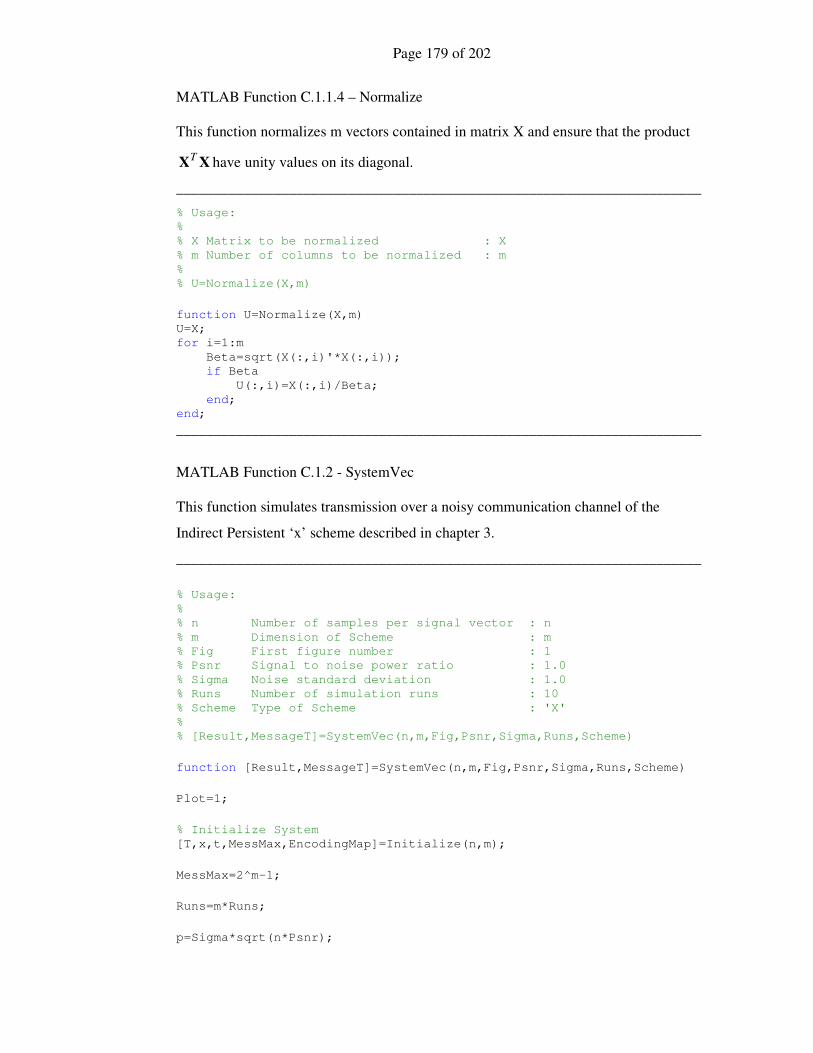
Page 179 of 202
MATLAB Function C.1.1.4 – Normalize
This function normalizes m vectors contained in matrix X and ensure that the product
XXT have unity values on its diagonal.
______________________________________________________________________
% Usage: % % X Matrix to be normalized : X % m Number of columns to be normalized : m % % U=Normalize(X,m)
function U=Normalize(X,m) U=X; for i=1:m Beta=sqrt(X(:,i)'*X(:,i)); if Beta U(:,i)=X(:,i)/Beta; end; end;
______________________________________________________________________
MATLAB Function C.1.2 - SystemVec
This function simulates transmission over a noisy communication channel of the
Indirect Persistent ‘x’ scheme described in chapter 3.
______________________________________________________________________
% Usage: % % n Number of samples per signal vector : n % m Dimension of Scheme : m % Fig First figure number : 1 % Psnr Signal to noise power ratio : 1.0 % Sigma Noise standard deviation : 1.0 % Runs Number of simulation runs : 10 % Scheme Type of Scheme : 'X' % % [Result,MessageT]=SystemVec(n,m,Fig,Psnr,Sigma,Runs,Scheme)
function [Result,MessageT]=SystemVec(n,m,Fig,Psnr,Sigma,Runs,Scheme)
Plot=1;
% Initialize System [T,x,t,MessMax,EncodingMap]=Initialize(n,m);
MessMax=2^m-1;
Runs=m*Runs;
p=Sigma*sqrt(n*Psnr);
Page 180 of 202
MessageT=zeros(Runs+1,1); MessageR=zeros(Runs+1,1); MessageError=zeros(Runs+1,1); Mt=zeros(Runs+1,1); Mr=zeros(Runs+1,1); Me=zeros(Runs+1,1);
Xt =zeros(n,m);
Zr =zeros(n,m); zt =zeros(n,1);
st =zeros(n,1);
Count=1; Error=1; Result=0;
% To simulate transmission delay % run receive code first while Runs
% Calculate Noise Matrices nq=Sigma*randn(n,1); ns=Sigma*randn(n,1);
% Decode Message if Scheme == 'x' zr=zt+nq; sr=st+ns;
Zr=[zr Zr(:,1:m-1)];
[U,Betat]=GramSchmidt(m,Zr); Qr=U*p;
if Plot figure(Fig+4); plot(Zr); str=sprintf('Persistent Received Z Matrix Balanced
Sequences'); title(str); xlabel('Samples'); nstr=sprintf('%s.fig',str); saveas(gcf,nstr); nstr=sprintf('%s.bmp',str); saveas(gcf,nstr); figure(Fig+5); plot(sr); str=sprintf('Received s Vector Encoded Sequence'); title(str); xlabel('Samples'); nstr=sprintf('%s.fig',str); saveas(gcf,nstr); nstr=sprintf('%s.bmp',str); saveas(gcf,nstr); end;
else
Page 181 of 202
return; end;
cr=inv(Qr'*Qr)*Qr'*sr;
c=cr; for i=1:m if c(i) < 0.0 c(i)=-1/sqrt(m); else c(i)=1/sqrt(m); end; end; for kk=1:2^m if c==(EncodingMap(:,kk)/sqrt(m)) Mr(Count)=kk-1; break; end; end;
MessageR(Count)=Mr(Count);
% Error calculation if Count > 1 MessageError(Count)=MessageT(Count-1)-MessageR(Count); Me(Count)=Mt(Count-1)-Mr(Count); end;
if MessageError(Count) if Error == 1 Result=[Count MessageError(Count)/MessMax Betat']; else Result=[Result;[Count MessageError(Count)/MessMax
Betat']]; end; Error=Error+1; end;
if Plot figure(Fig+6); stairs(MessageT); str=sprintf('Transmitted 4 Bit Messages'); title(str); xlabel('Samples'); nstr=sprintf('%s.fig',str); saveas(gcf,nstr); nstr=sprintf('%s.bmp',str); saveas(gcf,nstr); figure(Fig+7); stairs(MessageR); str=sprintf('Received 4 Bit Messages'); title(str); xlabel('Symbols'); nstr=sprintf('%s.fig',str); saveas(gcf,nstr); nstr=sprintf('%s.bmp',str); saveas(gcf,nstr); figure(Fig+8); stairs(MessageError); str=sprintf('Transmitted-Received 4 Bit Message Errors');

Page 182 of 202
title(str); xlabel('Symbols'); nstr=sprintf('%s.fig',str); saveas(gcf,nstr); nstr=sprintf('%s.bmp',str); saveas(gcf,nstr); end;
% Generate m level message MessageT(Count)=floor(MessMax*rand); R=MessageT(Count); Mt(Count)=R;
% Encode message ct = EncodingMap(:,Mt(Count)+1)/sqrt(m);
% Create Reference [xt,x]=Chaos(n,1,x,T); if Plot figure(Fig); plot(xt); str=sprintf('x Vector Chaotic Sequence'); title(str); xlabel('Samples'); nstr=sprintf('%s.fig',str); saveas(gcf,nstr); nstr=sprintf('%s.bmp',str); saveas(gcf,nstr);
end;
Xt=[xt Xt(:,1:m-1)];
zt=Normalize(xt,1)*p; [Ut,Betat]=GramSchmidt(m,Xt); Qt=Ut*p; st=Qt*ct;
if Plot figure(Fig+1); plot(Xt); str=sprintf('Persistent X Matrix Chaotic Sequence'); title(str); xlabel('Samples'); nstr=sprintf('%s.fig',str); saveas(gcf,nstr); nstr=sprintf('%s.bmp',str); saveas(gcf,nstr); figure(Fig+2); plot(Ut); str=sprintf('U Matrix Orthogonal Sequences'); title(str); xlabel('Samples'); nstr=sprintf('%s.fig',str); saveas(gcf,nstr); nstr=sprintf('%s.bmp',str); saveas(gcf,nstr); figure(Fig+3); plot(st); str=sprintf('s Vector Encoded Message Sequence');

Page 183 of 202
title(str); xlabel('Samples'); nstr=sprintf('%s.fig',str); saveas(gcf,nstr); nstr=sprintf('%s.bmp',str); saveas(gcf,nstr); end;
Count=Count+1; Runs=Runs-1; end;
______________________________________________________________________
C.2 BER Simulation MATLAB Function Listings
MATLAB Function C.2.1 – Ugen
This function simulates the BER v snrP [dB] noise behaviour of the Direct ‘U’ Scheme
______________________________________________________________________
% Usage: % % n An array of samples per signal vector : [8 32 128] % PsnrLimits An array of limits for Psnr : [0.01 100] % PsnrCount Number of points over PsnrLimits range : 100 % SimCount Number of simulation runs : 10000 % m_bits Array of dimension and bits : [2 4] % out Rate of plot output :
SimCount/100 % % [BER,P,Psnr]=Ugen(n,PsnrLimits,PsnrCount,SimCount,m_bits,out)
function [BER,P,Psnr]=Ugen(n,PsnrLimits,PsnrCount,SimCount,m_bits,out)
% Variable samples of data Num_n=max(size(n));
% Power Ratio Logarithmic Vector v=nthroot(PsnrLimits(2)/PsnrLimits(1),PsnrCount-1); Psnr=zeros(PsnrCount,1); Psnr(1)=PsnrLimits(1); for ii=2:PsnrCount Psnr(ii)=Psnr(ii-1)*v; end;
% Determine m and bits variables Size_M_Bits = size(m_bits); Dims = Size_M_Bits(1);
%Probability matrix P=zeros(PsnrCount,Num_n,Dims); BER=P;
for y=1:Dims

Page 184 of 202
% Dimension and Bits m=m_bits(y,1); bits=m_bits(y,2);
% Number of symbols mu=2^bits;
% Typical c vector c=zeros(m,1); if m==2 c=[real(exp(i*pi/mu));imag(exp(i*pi/mu))]; else for km=1:m c(km)=1/sqrt(m); end; end;
% Identity matrix Im Im=eye(m);
% Set random number state randn('state',0);
% Type of bit error calculation Direct = 0;
% SimCount simulation runs for ii=1:SimCount % For each data sample length for kk=1:Num_n E=randn(n(kk),m); Emm=E(1:m,1:m); e=randn(n(kk),1); em=e(1:m,1);
% Over the range for k=1:PsnrCount QTQ=n(kk)*Psnr(k)*Im+sqrt(n(kk)*Psnr(k))
*(Emm'+Emm)+E'*E; QTs=n(kk)*Psnr(k)*c+sqrt(n(kk)*Psnr(k))
*(Emm'*c+em)+E'*e;
cest=inv(QTQ)*QTs;
if Direct==1 for km=1:m if cest(km)<0 P(k,kk,y)=P(k,kk,y)+1/SimCount/m; BER(:,:,y)=P(:,:,y); end; end; else for km=1:m if cest(km)<0 P(k,kk,y)=P(k,kk,y)+1/SimCount; BER(:,:,y)=1.-nthroot(1.-P(:,:,y),bits); break; end;
Page 185 of 202
end; end; end; end;
% Plot output if (mod(ii,out)==0) str=sprintf('%d Dimension %d Symbols : %d%c
Complete',m,mu,floor(100*ii/SimCount),'%'); if Dims==1 semilogy(10*log10(Psnr),[SimCount*BER(:,:,1)/ii]); end; if Dims==2 semilogy(10*log10(Psnr),[SimCount*BER(:,:,1)/ii
SimCount*BER(:,:,2)/ii]); end; if Dims>=3 semilogy(10*log10(Psnr),[BER(:,:,1) BER(:,:,2)
BER(:,:,3)]); end; title(str); ylim([0.0001 1]); xlim([-20 20]); xlabel('Psnr[dB]'); ylabel('BER'); pause(0.01); end; end; end;
______________________________________________________________________
MATLAB Function C.2.2 - Xgen
This function simulates the BER v snrP [dB] noise behaviour of the Indirect ‘X’ Scheme
______________________________________________________________________ % Usage: % % WForm Character specification for W matrix : 'A' % n An array of samples per signal vector : [8 32 128] % PsnrLimits An array of limits for Psnr : [0.01 100] % PsnrCount Number of points over PsnrLimits range : 100 % SimCount Number of simulation runs : 10000 % m_bits Array of dimension and bits : [2 4] % out Rate of plot output : SimCount/100 % % [BER,P,Psnr]=Xgen(WForm,n,PsnrLimits,PsnrCount,SimCount,m_bits,out)
function
[BER,P,Psnr]=Xgen(WForm,n,PsnrLimits,PsnrCount,SimCount,m_bits,out)
% Variable samples of data Num_n=max(size(n));
% Power Ratio Vector v=nthroot(PsnrLimits(2)/PsnrLimits(1),PsnrCount-1); Psnr=zeros(PsnrCount,1); Psnr(1)=PsnrLimits(1);

Page 186 of 202
for ii=2:PsnrCount Psnr(ii)=Psnr(ii-1)*v; end;
% Determine m and bits variables Size_M_Bits=size(m_bits); Dims=Size_M_Bits(1);
%Probability matrix P=zeros(PsnrCount,Num_n,Dims); BER=P;
for y=1:Dims
m=m_bits(y,1); bits=m_bits(y,2);
% Number of symbols mu=2^bits;
% Typical c vector c=zeros(m,1); if m==2 c=[real(exp(i*pi/mu));imag(exp(i*pi/mu))]; else for km=1:m c(km)=1/sqrt(m); end; end;
% Identity matrix Im Im=eye(m);
% Set random number state randn('state',0);
% Scheme I W=Im;
% Scheme A if WForm=='A' for jj=1:m for ii=1:jj W(ii,jj)=1.0/sqrt(jj); end; end; end;
% Scheme B if WForm=='B' W=[1.0000 0.1481 -0.1345 0.1205; 0.0000 0.9890 0.8609 0.7699; -0.0000 -0.0000 0.4907 0.3383; 0.0000 0.0000 0.0000 0.5276];
W=W(1:m,1:m); end;
% Scheme C
Page 187 of 202
if WForm=='C' W=zeros(m,m); for jj=1:m W(1,jj)=1.0; end; end;
% SimCount simulation runs for ii=1:SimCount % For each data sample length for kk=1:Num_n U=[Im;zeros(n(kk)-m,m)]; E=randn(n(kk),m); Emm=E(1:m,1:m); e=randn(n(kk),1); em=e(1:m,1);
% Over the range for k=1:PsnrCount A=sqrt(n(kk)*Psnr(k))*U*W+E; [Ub,Beta] = GramSchmidt(m,A); QTQ=n(kk)*Psnr(k)*Im; QTs=n(kk)*Psnr(k)*Ub'*U*c+sqrt(n(kk)*Psnr(k))*Ub'*e;
cest=inv(QTQ)*QTs;
if m==2 Theta=atan2(cest(2),cest(1)); if Theta<0 || Theta>2*pi/mu P(k,kk,y)=P(k,kk,y)+1/SimCount; BER(:,:,y)=1.-nthroot(1.-P(:,:,y),bits); end; else for km=1:m if cest(km)<0 P(k,kk,y)=P(k,kk,y)+1/SimCount; BER(:,:,y)=1.-nthroot(1.-P(:,:,y),bits); break; end; end; end; end; end;
% Plot output if (mod(ii,out)==0) str=sprintf('%d Dimension %d Symbols : %d%c
Complete',m,mu,floor(100*ii/SimCount),'%'); if Dims==1 semilogy(10*log10(Psnr),[SimCount*BER(:,:,1)/ii]); end; if Dims==2 semilogy(10*log10(Psnr),[SimCount*BER(:,:,1)/ii
SimCount*BER(:,:,2)/ii]); end; if Dims>=3 semilogy(10*log10(Psnr),[BER(:,:,1) BER(:,:,2)
BER(:,:,3)]); end; title(str);

Page 188 of 202
ylim([0.0001 1]); xlim([-20 20]); xlabel('Psnr[dB]'); ylabel('BER'); pause(0.01); end; end; end;
______________________________________________________________________
MATLAB Function C.2.3 - EUgen
This function simulates the BER v 0N
Eb [dB] noise behaviour of the Direct ‘U’ Scheme
______________________________________________________________________ % Usage: % % n An array of samples per signal vector : [8 32 128] % EbNoLimits An array of limits for EbNo : [0.01 100] % EbNoCount Number of points over EbNoLimits range : 100 % SimCount Number of simulation runs : 10000 % m_bits Array of dimension and bits : [2 4] % out Rate of plot output : SimCount/100 % % [BER,P,Psnr]=EUgen(n,EbNoLimits,EbNoCount,SimCount,m_bits,out)
function [BER,P,EbNo]=EUgen(n,EbNoLimits,EbNoCount,SimCount,
m_bits,out)
% Variable samples of data Num_n=max(size(n));
% Power Ratio Vector v=nthroot(EbNoLimits(2)/EbNoLimits(1),EbNoCount-1); EbNo=zeros(EbNoCount,1); EbNo(1)=EbNoLimits(1); for ii=2:EbNoCount EbNo(ii)=EbNo(ii-1)*v; end;
% Determine m and bits variables Size_M_Bits=size(m_bits); Dims=Size_M_Bits(1);
%Probability matrix P=zeros(EbNoCount,Num_n,Dims); BER=P;
for y=1:Dims
m=m_bits(y,1); bits=m_bits(y,2);

Page 189 of 202
% Number of symbols mu=2^bits;
% Typical c vector c=zeros(m,1); if m==2 c=[real(exp(i*pi/mu));imag(exp(i*pi/mu))]; else for km=1:m c(km)=1/sqrt(m); end; end;
% Identity matrix Im Im=eye(m);
% Set random number state randn('state',0);
% SimCount simulation runs for ii=1:SimCount % For each data sample length for kk=1:Num_n E=randn(n(kk),m); Emm=E(1:m,1:m); e=randn(n(kk),1); em=e(1:m,1);
% Over the range for k=1:EbNoCount Psnr=m*EbNo(k)/n(kk); QTQ=Psnr*n(kk)*Im+sqrt(Psnr)*sqrt(n(kk))
*(Emm'+Emm)+E'*E; QTs=Psnr*n(kk)*c+sqrt(Psnr)*sqrt(n(kk))
*(Emm'*c+em)+E'*e;
cest=inv(QTQ)*QTs;
if m==2 Theta=atan2(cest(2),cest(1)); if Theta<0 || Theta>2*pi/mu P(k,kk,y)=P(k,kk,y)+1/SimCount; BER(:,:,y)=1.-nthroot(1.-P(:,:,y),bits); end; else for km=1:m if cest(km)<0 P(k,kk,y)=P(k,kk,y)+1/SimCount; BER(:,:,y)=1.-nthroot(1.-P(:,:,y),bits); break; end; end; end; end; end;
% Plot Output if (mod(ii,out)==0) str=sprintf('%d Dimension %d Symbols : %d%c
Complete',m,mu,100*ii/SimCount,'%');

Page 190 of 202
if Dims==1 semilogy(10*log10(EbNo),[SimCount*BER(:,:,1)/ii]); end; if Dims==2 semilogy(10*log10(EbNo),[SimCount*BER(:,:,1)/ii
SimCount*BER(:,:,2)/ii]); end; if Dims>=3 semilogy(10*log10(EbNo),[BER(:,:,1) BER(:,:,2)
BER(:,:,3)]); end; title(str); ylim([0.0001 1]); xlim([0 20]); xlabel('Eb/No[dB]'); ylabel('BER'); pause(0.01); end; end; end;
______________________________________________________________________
MATLAB Function C.2.4 - EXgen
This function simulates the BER v 0N
Eb [dB] noise behaviour of the Direct ‘X’ Scheme
______________________________________________________________________ % Usage: % % WForm Character specification for W matrix : 'A' % n An array of samples per signal vector : [8 32 128] % EbNoLimits An array of limits for EbNo : [0.01 100] % EbNoCount Number of points over EbNoLimits range : 100 % SimCount Number of simulation runs : 10000 % m_bits Array of dimension and bits : [2 4] % out Rate of plot output : SimCount/100 % % [BER,P,Psnr]=EXgen(WForm,n,EbNoLimits,EbNoCount,SimCount,m_bits,out)
function
[BER,P,EbNo]=EXgen(WForm,n,EbNoLimits,EbNoCount,SimCount,m_bits,out)
% Variable samples of data Num_n=max(size(n));
% Power Ratio Vector v=nthroot(EbNoLimits(2)/EbNoLimits(1),EbNoCount-1); EbNo=zeros(EbNoCount,1); EbNo(1)=EbNoLimits(1); for ii=2:EbNoCount EbNo(ii)=EbNo(ii-1)*v; end;
% Determine m and bits variables Size_M_Bits=size(m_bits);

Page 191 of 202
Dims=Size_M_Bits(1);
%Probability matrix P=zeros(EbNoCount,Num_n,Dims); BER=P;
for y=1:Dims
m=m_bits(y,1); bits=m_bits(y,2);
% Number of symbols mu=2^bits;
% Typical c vector c=zeros(m,1); if m==2 c=[real(exp(i*pi/mu));imag(exp(i*pi/mu))]; else for km=1:m c(km)=1/sqrt(m); end; end;
% Identity matrix Im Im=eye(m);
% Set random number state randn('state',0);
% Scheme I W=Im;
% Scheme A if WForm=='A' for jj=1:m for ii=1:jj W(ii,jj)=1.0/sqrt(jj); end; end; end;
% Scheme B if WForm=='B' W=[1.0000 0.1481 -0.1345 0.1205; 0.0000 0.9890 0.8609 0.7699; -0.0000 -0.0000 0.4907 0.3383; 0.0000 0.0000 0.0000 0.5276];
W=W(1:m,1:m); end;
% Scheme C if WForm=='C' W=zeros(m,m); for jj=1:m W(1,jj)=1.0; end; end;
Page 192 of 202
% SimCount simulation runs for ii=1:SimCount % For each data sample length for kk=1:Num_n U=[Im;zeros(n(kk)-m,m)]; E=randn(n(kk),m); Emm=E(1:m,1:m); e=randn(n(kk),1); em=e(1:m,1);
% Over the range for k=1:EbNoCount Psnr=m*EbNo(k)/n(kk); A=sqrt(n(kk)*Psnr)*U*W+E; [Ub,Beta] = GramSchmidt(m,A); QTQ=n(kk)*Psnr*Im; QTs=n(kk)*Psnr*Ub'*U*c+sqrt(n(kk)*Psnr)*Ub'*e;
cest=inv(QTQ)*QTs;
if m==2 Theta=atan2(cest(2),cest(1)); if Theta<0 || Theta>2*pi/mu P(k,kk,y)=P(k,kk,y)+1/SimCount; BER(:,:,y)=1.-nthroot(1.-P(:,:,y),bits); end; else for km=1:m if cest(km)<0 P(k,kk,y)=P(k,kk,y)+1/SimCount; BER(:,:,y)=1.-nthroot(1.-P(:,:,y),bits); break; end; end; end; end; end;
%Plot Outputs if (mod(ii,out)==0) str=sprintf('%d Dimension %d Symbols : %d%c
Complete',m,mu,100*ii/SimCount,'%'); if Dims==1 semilogy(10*log10(EbNo),[SimCount*BER(:,:,1)/ii]); end; if Dims==2 semilogy(10*log10(EbNo),[SimCount*BER(:,:,1)/ii
SimCount*BER(:,:,2)/ii]); end; if Dims>=3 semilogy(10*log10(EbNo),[BER(:,:,1) BER(:,:,2)
BER(:,:,3)]); end; title(str); ylim([0.0001 1]); xlim([0 20]); xlabel('Eb/No[dB]'); ylabel('BER');

Page 193 of 202
pause(0.01); end; end; end;
______________________________________________________________________

Page 194 of 202
ρ r
z θ
Appendix D
D.1 Hypersphere Volume Calculations
Figure D.1.1
Calculation of Dimension m Hyperspherical Volume
Derivation D.1.1
______________________________________________________________________
Consider the volume of an m dimensional hypersphere expressed as a function of
hyperspherical volumes of dimension 1−m , as illustrated in the figure (D.1.1)
above
∫−
−=
r
r
mm dzVrV )()( 1 ρ (D.1.1)
Making the following substitutions θcosrz = , θθdrdz sin−= and θρ sinr=
yields

Page 195 of 202
θθθ
π∫−
−−=
0
1 sin)sin()( drrVrV mm
θθθ
π
∫ −=
0
1 sin)sin( drVr m (D.1.2)
Now the volume of the hypersphere is clearly proportional to the radius r raised to
the mth
power. That is
mm rmrV )()( α= (D.1.3)
where the )(mα term is a constant dependent on the dimension m. From equation
(D.1.2) the reduced radius θρ sinr= can be used to express the 1−m
dimensional volume in the same way, using the constant term for the reduced
dimension as
θαθ sin)1()sin( 11
−− −= m
m rmrV (D.1.4)
Substituting (D.1.3) and (D.1.4) into (D.1.2) gives a dimensionally recursive
expression for the constant term, that is
θθθαα
π
∫ −−−=
0
11 sinsin)1()( drmrrmmmm (D.1.5)
And cancelling like powers of the radius r gives
θθαα
π
∫−=
0
sin)1()( dmmm (D.1.6)
The integral sine function can be expressed in a recursive form as follows
θθ
π
∫=
0
sin)( dmIm (D.1.7)
then (D.1.6) becomes
)()1()( mImm −= αα (D.1.8)
Now )(mI can be rewritten as

Page 196 of 202
θθθ
π
∫ −=
0
22 sinsin)( dmIm (D.1.9)
And integrating by parts gives
θθθθ
π
∫ −− −=
0
222 sincossin)( dmImm
θθθθ
π
∫ −⋅−−=
0
2sincoscos)2( dmIm
θθθθ
θ
ππ
∫ ⋅−
−
−⋅−−=
−−
0
1
0
1
sin)1(
sin
)1(
sincos)2( d
mmmI
mm
)()1(
1)2( mI
mmI
−−−= (D.1.10)
And finally by rearranging produces a recursive formula for the sine integral
function as
)2()1(
)( −−
= mIm
mmI (D.1.11)
For the next part of the derivation we will need two special values of this function
these are I(0) and I(1). These are simply calculated to yield
πθ
π
== ∫0
)0( dI and 2sin)1(
0
== ∫π
θθdI (D.1.12)
Two other values are also required namely )0(α and )1(α . Now we know that
πα =)2( because the volume of a two dimensional hypersphere is 2rπ . So from
(D.1.8) and (D.1.11) these values are
2)0(
)2(
)2(
)2()1(
21
===II
ααα and 1
)1(
)1()0( ==
I
αα
Next reconsider equation (D.1.8) and further expand it until 1=m
)1()()( −= mmIm αα
)2()1()( −−= mmImI α
)0()1()( αImI L= (D.1.13)
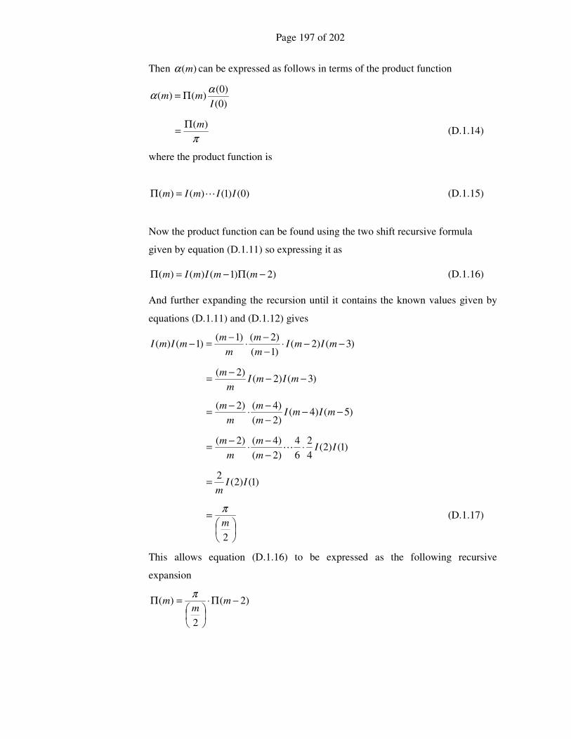
Page 197 of 202
Then )(mα can be expressed as follows in terms of the product function
)0(
)0()()(
Imm
αα Π=
π
)(mΠ= (D.1.14)
where the product function is
)0()1()()( IImIm L=Π (D.1.15)
Now the product function can be found using the two shift recursive formula
given by equation (D.1.11) so expressing it as
)2()1()()( −Π−=Π mmImIm (D.1.16)
And further expanding the recursion until it contains the known values given by
equations (D.1.11) and (D.1.12) gives
)3()2()1(
)2()1()1()( −−⋅
−
−⋅
−=− mImI
m
m
m
mmImI
)3()2()2(
−−−
= mImIm
m
)5()4()2(
)4()2(−−
−
−⋅
−= mImI
m
m
m
m
)1()2(4
2
6
4
)2(
)4()2(II
m
m
m
m⋅
−
−⋅
−= L
)1()2(2
IIm
=
=
2
m
π (D.1.17)
This allows equation (D.1.16) to be expressed as the following recursive
expansion
)2(
2
)( −Π⋅
=Π m
mm
π

Page 198 of 202
)4(
2
2
2
−Π
−⋅
= m
mm
ππ
)0(
2
2
2
4
2
2
2
Π
−⋅
−⋅
=
ππππL
mmm (D.1.18)
The resultant equation (D.1.18) can now be expressed in terms of the gamma
function to in place of the factorial term and substituting π==Π )0()0( I yields
)0(
2
)(
!2
Π
=Π
mm
m
π
!2
12
=
+
m
m
π
+Γ
=Π+
12
)(
12
mm
m
π (D.1.19)
The volume of the hypersphere can now be expressed as follows using equations
(D.1.3) (D.1.14) and (D.1.19) as
mm r
mrV
m
⋅
+Γ
=
12
)(2π
(D.1.20)
Now for even values of m, the gamma function can easily be evaluated since at
integer values it merely becomes a factorial, that is ( ) !1 kk =+Γ . However for odd
values of m the gamma function has to be evaluated at values halfway between
integers as follows
−Γ⋅
=
+Γ 1
221
2
mmm
Γ⋅⋅
−⋅
−⋅
=
2
1
2
1
2
3
2
4
2
2
2L
mmm (D.1.21)
Now in order to find
Γ
2
1we require Euler’s reflection formula that is
Page 199 of 202
zzz
π
π
sin)1()( =−ΓΓ (D.1.22)
So for 2
1=z the result is
=
Γ
2sin
2
12
π
π (D.1.23)
This yields the well known result
21
2
1π=
Γ (D.1.24)
Allowing the volume for any dimension m to be calculated using equation
(D.1.20).
______________________________________________________________________
D.2 Maxima of Comparative Function
Derivation D.2.1
______________________________________________________________________
Recall the comparative function given by result (D.2.5)
2
21
12 m
mC
m
m ⋅
+Γ
=−
π
The differential of this with respect to the dimension m is derived and equated to
zero to find the maxima as
0
21
21
2221
2
12
12
=
+Γ
+Γ⋅⋅−
⋅⋅
+Γ
=
−−
m
m
dm
dmm
dm
dm
dm
dC
mm
m
ππ
(D.2.1)
Evaluating intermediate functional derivatives for equation (D.2.1) yields
Page 200 of 202
12
12
12
2
1
22
−−−+
⋅=
⋅
mmm
dm
dmm
dm
dπππ (D.2.2)
And
12
12 log
2
1 −−⋅=
m
e
m
dm
dπππ (D.2.3)
Now consider the digamma function which is defined as
)(
)(
)(log)(m
mdx
d
mdm
dm e
Γ
Γ=Γ=ϕ (D.2.4)
And rearranging this allows the expression of the gamma function derivative in
equation (D.2.1) to be expressed as
)()()( mmmdm
dϕΓ=Γ (D.2.5)
+
+Γ=
+Γ
21
21
2
1
21
mmm
dm
dϕ (D.2.6)
Substituting (D.2.2), (D.2.3) and (D.2.6) into equation (D.2.1) gives
the following result
+
+Γ⋅⋅=
+⋅⋅
+Γ
−−−
21
21
2
1
22
1log
2
1
221
12
12
12
mmmmmmmm
e ϕππππ
which simplifies to
+=
+
21
21log
2
mmme ϕπ
and finally rearranges to give
m
me
2log
21 =−
+ πϕ (D.2.7)
______________________________________________________________________
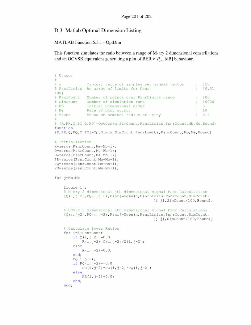
Page 201 of 202
D.3 Matlab Optimal Dimension Listing
MATLAB Function 5.3.1 - OptDim
This function simulates the ratio between a range of M-ary 2 dimensional constellations
and an OCVSK equivalent generating a plot of BER v snrP [dB] behaviour.
______________________________________________________________________
% Usage: % % n Typical value of samples per signal vector : 128 % PsnrLimits An array of limits for Psnr : [0.01
100] % PsnrCount Number of points over PsnrLimits range : 100 % SimCount Number of simulation runs : 10000 % Mb Initial Dimensional order : 3 % Me Rate of plot output : 10 % Bound Bound on nominal radius of unity : 0.4 % % [R,PR,Q,PQ,O,PO]=OptDim(n,SimCount,PsnrLimits,PsnrCount,Mb,Me,Bound) function
[R,PR,Q,PQ,O,PO]=OptDim(n,SimCount,PsnrLimits,PsnrCount,Mb,Me,Bound)
% Initialization R=zeros(PsnrCount,Me-Mb+1); Q=zeros(PsnrCount,Me-Mb+1); O=zeros(PsnrCount,Me-Mb+1); PR=zeros(PsnrCount,Me-Mb+1); PQ=zeros(PsnrCount,Me-Mb+1); PO=zeros(PsnrCount,Me-Mb+1);
for j=Mb:Me
figure(1); % M-Ary 2 dimensional jth dimensional signal Psnr Calculations [Q(:,j-2),PQ(:,j-2),Psnr]=Ugen(n,PsnrLimits,PsnrCount,SimCount,
[2 j],SimCount/100,Bound);
% OCVSK j dimensional jth dimensional signal Psnr Calculations [O(:,j-2),PO(:,j-2),Psnr]=Ugen(n,PsnrLimits,PsnrCount,SimCount,
[j j],SimCount/100,Bound);
% Calculate Power Ratios for i=1:PsnrCount if Q(i,j-2)~=0.0 R(i,j-2)=O(i,j-2)/Q(i,j-2); else R(i,j-2)=0.0; end; PQ(i,j-2); if PQ(i,j-2)~=0.0 PR(i,j-2)=PO(i,j-2)/PQ(i,j-2); else PR(i,j-2)=0.0; end; end;

Page 202 of 202
% Display figure(2); semilogy(10*log10(Psnr),R(:,1:j-2)); figure(3); semilogy(10*log10(Psnr),PR(:,1:j-2));
end;
______________________________________________________________________