appendix g wolf creek qual2k model report · kootenai-fisher project area metals, nutrients,...
TRANSCRIPT
Kootenai-Fisher Project Area Metals, Nutrients, Sediment, & Temperature TMDLs - Appendix G
5/7/14 Final G-1
APPENDIX G – WOLF CREEK QUAL2K MODEL REPORT
TABLE OF CONTENTS
Acronyms and Abbreviations .................................................................................................................... G-5
Units of Measure....................................................................................................................................... G-5
Executive Summary ................................................................................................................................... G-6
G1.0 Introduction ...................................................................................................................................... G-6
G2.0 Background ....................................................................................................................................... G-6
G2.1 Problem Statement ...................................................................................................................... G-7
G2.2 Montana Temperature Standard ................................................................................................. G-7
G2.3 Factors Potentially Influencing Stream Temperature .................................................................. G-8
G2.4 Stream Temperature Data ............................................................................................................ G-8
G2.5 Temperature Data Analysis .......................................................................................................... G-9
G3.0 QUAL2K Model Development .................................................................................................... G-15
G3.1 Model Framework ...................................................................................................................... G-15
G3.2 Model Configuration and Setup ................................................................................................. G-15
G3.2.1 Modeling Time Period ......................................................................................................... G-15
G3.2.2 Segmentation ...................................................................................................................... G-16
G3.2.2 Hydraulics ............................................................................................................................ G-16
G3.2.4 Boundary Conditions ........................................................................................................... G-17
G3.2.5 Meteorological Data ............................................................................................................ G-20
G3.2.6 Shade Data ........................................................................................................................... G-20
G3.3 Model Evaluation Criteria ........................................................................................................... G-21
G3.4 Model Calibration and Validation............................................................................................... G-21
G4.0 Model Scenarios and Results .......................................................................................................... G-29
G4.1 Critical Existing Condition Scenario (Baseline) ........................................................................... G-29
G4.2 Water Use Scenario .................................................................................................................... G-32
G4.3 Shade Scenario ........................................................................................................................... G-33
G4.4 Improved Flow and Shade Scenario ........................................................................................... G-35
G5.0 Assumptions and Uncertainty ........................................................................................................ G-36
G6.0 Model Use and Limitations ............................................................................................................. G-38
G7.0 Conclusions ..................................................................................................................................... G-39
G8.0 References ...................................................................................................................................... G-41
Attachment G-1 - Factors Potentially Influencing Stream Temperature in Wolf Creek ......................... G-42
Kootenai-Fisher Project Area Metals, Nutrients, Sediment, & Temperature TMDLs - Appendix G
5/7/14 Final G-2
G1-1.0 Introduction ................................................................................................................................ G-42
G1-2.0 Climate ........................................................................................................................................ G-42
G1-3.0 Land Ownership and Land Use .................................................................................................... G-44
G1-4.0 Existing Riparian Vegetation ....................................................................................................... G-46
G1-5.0 Shade ........................................................................................................................................... G-47
G1-5.1 Measured Shade ..................................................................................................................... G-47
G1-5.2 Shade Modeling....................................................................................................................... G-48
G1-5.2.1 Available Data .................................................................................................................. G-48
G1-5.2.2 GIS Pre-Processing ............................................................................................................ G-48
G1-5.2.3 Riparian Input ................................................................................................................... G-48
G1-5.2.4 Shade Input ...................................................................................................................... G-49
G1-5.3 Shade Model Results ............................................................................................................... G-49
G1-6.0 Hydrology .................................................................................................................................... G-51
G1-7.0 Flow Modification ....................................................................................................................... G-53
G1-8.0 Point Sources ........................................................................................................................... G-54
LIST OF TABLES
Table G-1. EPA instantaneous water temperature measurements (°F), summer 2012 ........................... G-9 Table G-2. QUAL2K model flow and temperature inputs to Wolf Creek - Tributaries and withdrawal . G-19 Table G-3. QUAL2K model flow and temperature inputs to Wolf Creek - Diffuse sources .................... G-20 Table G-4. Temperature calibration and validation locations ................................................................ G-21 Table G-5. Solar radiation settings .......................................................................................................... G-26 Table G-6. Calibration statistics of observed versus predicted water temperatures ............................. G-28 Table G-7. Validation statistics of observed versus predicted water temperatures .............................. G-28 Table G-8. QUAL2K model scenarios for Wolf Creek .............................................................................. G-29 Table G1-1. Land cover types in the Wolf Creek riparian zone .............................................................. G-47 Table G1-2. Average shade per reach from Solar PathfinderTM measurements .................................... G-48 Table G1-3. Vegetation input values for the Shade Model .................................................................... G-49 Table G1-4. Shade model error statistics ................................................................................................ G-51 Table G1-5. EPA instantaneous flow measurements (cfs) on Wolf Creek in support of modeling ........ G-51 Table G1-6. EPA instantaneous flow measurements (cfs) on tributaries to Wolf Creek in support of modeling ................................................................................................................................................. G-51 Table G1-7. EPA instantaneous flow measurements (cfs) in support of other water quality studies .... G-51 Table G1-8. Points of diversion from Wolf Creek ................................................................................... G-54
LIST OF FIGURES
Figure G-1. Wolf Creek watershed ............................................................................................................ G-7 Figure G-2. Temperature loggers in the Wolf Creek watershed. .............................................................. G-9
Kootenai-Fisher Project Area Metals, Nutrients, Sediment, & Temperature TMDLs - Appendix G
5/7/14 Final G-3
Figure G-3. Box-and-whisker plots of DEQ temperature data, June 26 or July13 to September 17 or 19, 2012. ....................................................................................................................................................... G-11 Figure G-4. Daily maximum temperatures along Wolf Creek, upper half of the watershed, June 25, 2012 to September 24, 2012. .......................................................................................................................... G-12 Figure G-5. Daily maximum temperatures along Wolf Creek, lower half of the watershed, June 25, 2012 to September 24, 2012. .......................................................................................................................... G-13 Figure G-6. Daily maximum temperatures on the tributaries to Wolf Creek, June 25, 2012 to September 24, 2012. ................................................................................................................................................. G-14 Figure G-7. Wolf Creek modeling domain, logger locations, RAWS, and irrigation withdrawal. ........... G-16 Figure G-8. Wolf Creek channel elevation and slope representations. .................................................. G-17 Figure G-9. Diurnal temperature at the headwaters to Wolf Creek. ...................................................... G-18 Figure G-10. Observed and predicted flow (Q), velocity (U), and depth (H) on August 9, 2012 (calibration). ............................................................................................................................................ G-23 Figure G-11. Observed and predicted flow (Q), velocity (U), and depth (H) on September 16, 2012 (validation). ............................................................................................................................................. G-24 Figure G-12. Observed and predicted solar radiation on August 9, 2012 and September 16, 2012 (calibration and validation). .................................................................................................................... G-25 Figure G-13. Longitudinal profile of the temperature calibration (August 9, 2012). ............................. G-27 Figure G-14. Longitudinal profile of the temperature validation (September 16, 2012). ...................... G-27 Figure G-15. Monthly air temperature at Kalispell Glacier Park International Airport. ......................... G-31 Figure G-16. Simulated water temperature for the existing condition (August 8. 2012). ...................... G-32 Figure G-17. Simulated water temperatures for the critical existing critical condition (scenario 1) and 15-percent withdrawal reduction (scenario 2). ........................................................................................... G-33 Figure G-18. Effective shading along Wolf Creek for the critical existing condition and 50-foot buffer shade scenario. ....................................................................................................................................... G-34 Figure G-19. Simulated water temperatures for the critical existing condition (scenario 1) and shade with 50 feet buffer (scenario 3). ..................................................................................................................... G-34 Figure G-20. Simulated water temperature for the critical existing condition (scenario 1) and the improved flow and shade scenario (scenario 4). .................................................................................... G-35 Figure G-21. Instream temperature difference from critical existing condition (scenario 1) to the improved flow and shade scenario (scenario 4). .................................................................................... G-36 Figure G-22. Simulated daily maximum water temperatures from the critical existing condition (red; scenario 1) and improved flow and shade scenario (blue; scenario 4). ................................................. G-39 Figure G-23. Simulated water temperature reduction from the critical existing condition (scenario 1) to the improved flow and shade scenario (scenario 4). .............................................................................. G-40 Figure G-24. Shade deficit of the critical existing condition (scenario 1) from the improved flow and shade scenario (scenario 4). ................................................................................................................... G-40 Figure G1-1. Location of Wolf Creek watershed and nearby weather stations. .................................... G-43 Figure G1-2. Monthly average temperatures and precipitation at Hand Creek Weather Station. ........ G-43 Figure G1-3. Land ownership in the Wolf Creek watershed. .................................................................. G-44 Figure G1-5. Aerial imagery of the Wolf Creek watershed. .................................................................... G-45 Figure G1-6. Vegetation mapping example for Wolf Creek. ................................................................... G-46 Figure G1-7. EPA flow, shade, and continuous temperature monitoring locations. .............................. G-47 Figure G1-8. Longitudinal estimates of observed and simulated effective shade along Wolf Creek. .... G-50 Figure G1-9. Flow monitoring locations. ................................................................................................. G-52 Figure G1-10. Flow analysis with USGS gage 12302055 (Fisher River near Libby, MT). ......................... G-53 Figure G1-11. Surface and groundwater diversions in the Wolf Creek watershed. ............................... G-54

Kootenai-Fisher Project Area Metals, Nutrients, Sediment, & Temperature TMDLs - Appendix G
5/7/14 Final G-4
LIST OF ATTACHMENTS
Attachment G-1 - Factors Potentially Influencing Stream Temperature in Wolf Creek

Kootenai-Fisher Project Area Metals, Nutrients, Sediment, & Temperature TMDLs - Appendix G
5/7/14 Final G-5
ACRONYMS AND ABBREVIATIONS
AME Absolute Mean Error EPA Environmental Protection Agency (U.S.) DEQ Department of Environmental Quality (Montana) MRLC Multi-Resolution Land Characteristics Consortium NLCD National Land Cover Dataset NRCS Natural Resources Conservation Service (U.S. Department of Agriculture) QUAL2K River and Stream Water Quality Model REL Relative Error RM Rivermile TMDL Total Maximum Daily Load USFS U.S. Forest Service (U.S. Department of Agriculture) USGS U.S. Geological Survey (U.S. Department of the Interior) WRCC Western Regional Climate Center
UNITS OF MEASURE
°F degrees Fahrenheit cfs cubic feet per second MSL mean sea level RM river mile

Kootenai-Fisher Project Area Metals, Nutrients, Sediment, & Temperature TMDLs - Appendix G
5/7/14 Final G-6
EXECUTIVE SUMMARY
Wolf Creek is listed on the 2012 303(d) List as impaired because of elevated water temperatures. The cause of the impairment was attributed to channelization and highways, roads, bridges, and infrastructure (new construction). Field studies were carried out in 2012 to support water quality model development for the project. A QUAL2K water quality model was then developed for Wolf Creek to evaluate the impairment status and the effect that human sources have had on stream temperatures. The QUAL2K model was constructed, in part, using field collected data from the summer of 2012. Shadev3.0 models were also developed to assess shade conditions using previously collected field data. The calibrated and validated QUAL2K model met previously designated acceptance criteria. Once developed, various water temperature responses were evaluated for a range of potential watershed management activities. Four scenarios were evaluated:
• Scenario 1: Critical existing condition (i.e., the calibrated model with critical weather and low-flow conditions). This served as the baseline scenario from which to compare the other scenarios.
• Scenario 2: Critical existing conditions with a 15 percent reduction of water withdrawals. This is to simulate standards attainment regarding water conservation practices.
• Scenario 3: Critical existing condition with improved riparian vegetation in a 50-foot buffer. This is to simulate standards attainment regarding soil and land conservation practices.
• Scenario 4: An improved flow and shade scenario that combines the potential benefits associated with a 15 percent reduction in water withdrawals with a 50-foot vegetated buffer. This is to simulate full standards attainment via the use of all reasonable land, soil, and water conservation practices.
In comparison to scenario 1, the results ranged from almost no change in water temperatures (scenarios 2) to considerable reductions (scenarios 3 and 4). Scenario 4 resulted in overall reductions along the entire reach which ranged from 0.7° F to 7.8° F. Generally, small changes in shade or inflow had minimal effects on water temperatures while large increases in shade had considerable effects on water temperatures. The scenarios indicate the allowable human caused temperature change is being exceeded and support the impairment listing.
G1.0 INTRODUCTION
This appendix is based on a model report completed by Tetra Tech (2013) for a temperature model (QUAL2K) that was used to support TMDL development for Wolf Creek. Background information is provided in the following section (Section G.2). A summary of model set up, calibration, and validation is provided in Section G.3 and a series of model scenarios and results are presented in Section G.4.
G2.0 BACKGROUND
This section presents background information to support QUAL2K model development.
Kootenai-Fisher Project Area Metals, Nutrients, Sediment, & Temperature TMDLs - Appendix G
5/7/14 Final G-7
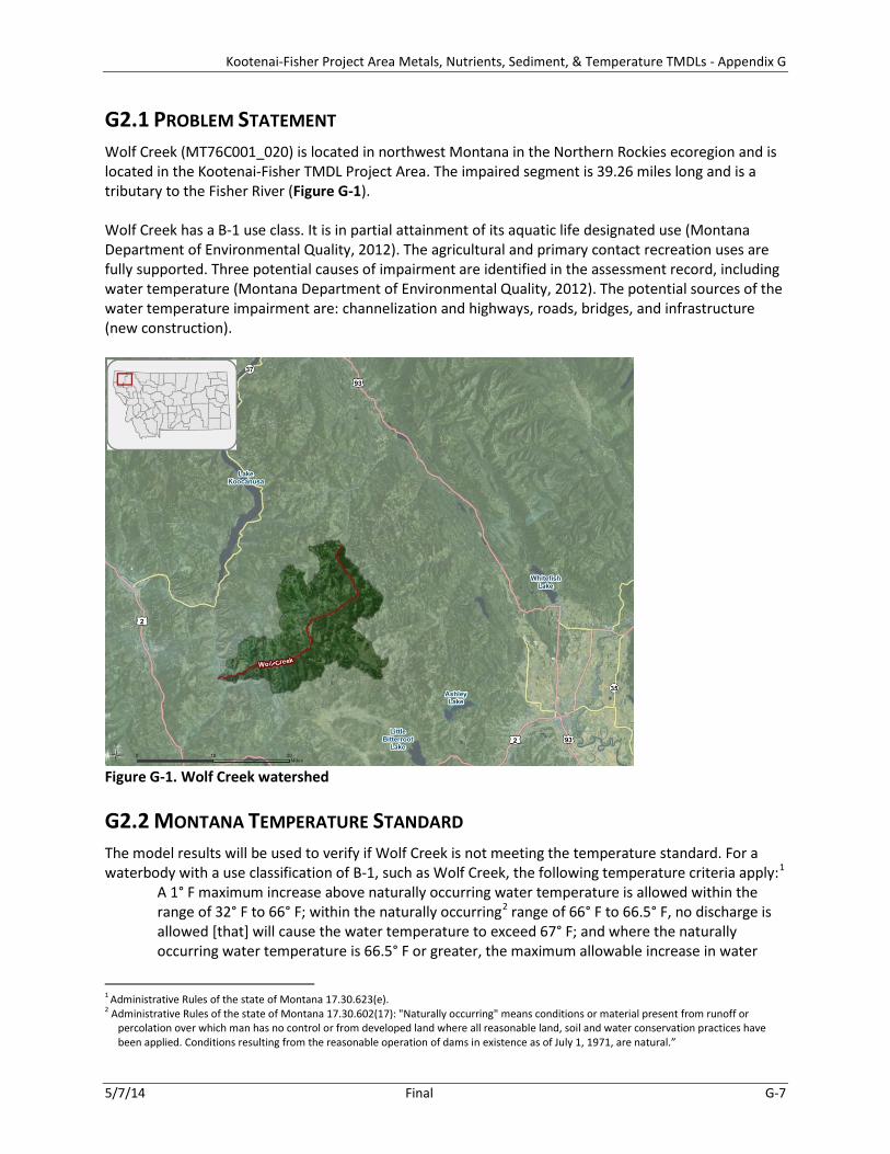
G2.1 PROBLEM STATEMENT Wolf Creek (MT76C001_020) is located in northwest Montana in the Northern Rockies ecoregion and is located in the Kootenai-Fisher TMDL Project Area. The impaired segment is 39.26 miles long and is a tributary to the Fisher River (Figure G-1). Wolf Creek has a B-1 use class. It is in partial attainment of its aquatic life designated use (Montana Department of Environmental Quality, 2012). The agricultural and primary contact recreation uses are fully supported. Three potential causes of impairment are identified in the assessment record, including water temperature (Montana Department of Environmental Quality, 2012). The potential sources of the water temperature impairment are: channelization and highways, roads, bridges, and infrastructure (new construction).
Figure G-1. Wolf Creek watershed
G2.2 MONTANA TEMPERATURE STANDARD The model results will be used to verify if Wolf Creek is not meeting the temperature standard. For a waterbody with a use classification of B-1, such as Wolf Creek, the following temperature criteria apply:1
A 1° F maximum increase above naturally occurring water temperature is allowed within the range of 32° F to 66° F; within the naturally occurring2 range of 66° F to 66.5° F, no discharge is allowed [that] will cause the water temperature to exceed 67° F; and where the naturally occurring water temperature is 66.5° F or greater, the maximum allowable increase in water
1 Administrative Rules of the state of Montana 17.30.623(e). 2 Administrative Rules of the state of Montana 17.30.602(17): "Naturally occurring" means conditions or material present from runoff or
percolation over which man has no control or from developed land where all reasonable land, soil and water conservation practices have been applied. Conditions resulting from the reasonable operation of dams in existence as of July 1, 1971, are natural.”

Kootenai-Fisher Project Area Metals, Nutrients, Sediment, & Temperature TMDLs - Appendix G
5/7/14 Final G-8
temperature is 0.5° F. A 2° F per-hour maximum decrease below naturally occurring water temperature is allowed when the water temperature is above 55° F. A 2° F maximum decrease below naturally occurring water temperature is allowed within the range of 55° F to 32° F.
G2.3 FACTORS POTENTIALLY INFLUENCING STREAM TEMPERATURE Stream temperature regimes are influenced by processes that are external to the stream as well as processes that occur within the stream and its associated riparian zone (Poole et al., 2001). Examples of factors external to the stream that can affect instream water temperatures include: topographic shade, land use/land cover (e.g., vegetation and the shading it provides, impervious surfaces), solar angle, meteorological conditions (e.g., precipitation, air temperature, cloud cover, relative humidity), groundwater exchange and temperature, and tributary inflow temperatures and volumes. The shape of the channel can also affect the temperature—wide shallow channels are more easily heated and cooled than deep, narrow channels. The amount of water in the stream is another factor influencing stream temperature regimes. Streams that carry large amounts of water resist heating and cooling, whereas temperature in small streams (or reduced flows) can be changed more easily. The following factors that may have an influence on stream temperatures in Wolf Creek were evaluated prior to model development and are further discussed in Attachment G-1:
• Local/regional climate • Land ownership • Land use • Riparian vegetation • Shade • Hydrology • Point sources
G2.4 STREAM TEMPERATURE DATA In 2012, EPA collected continuous temperature data at seven locations in Wolf Creek (sites WLFC-T0.1, WLFC-T0.2, WLFC-T1, WLFC-T1.5, WLFC-T2, WLFC-T2.5, and WLFC-T3) and at five tributary locations (BRSHC on Brush Creek, CALXC on Calx Creek, DRFKC on Dry Fork Creek, LWLFC on Little Wolf Creek, and RCHDC on Richard Creek) (Figure G-2). Data loggers recorded temperatures every one-half hour for approximately two months between June 26 or July 13, 20123 and September 17 or 19, 2012. Instantaneous water temperatures4 were recorded during logger deployment and retrieval (Table G-1). Plum Creek deployed temperature loggers at two locations in Wolf Creek. Both sites were upstream of the confluence with Dry Fork Creek and between EPA monitoring sites WLFC-T1 and WLFC-0.2. Additionally, a temperature logger was deployed in one location in Little Wolf Creek during the same time period (Figure G-2). Plum Creek’s loggers were deployed form June 20, 2012 to December 2, 2012. To provide a comparison to the EPA data, only the Plum Creek data collected between June 20 and September 19th are considered herein.
3 Temperature loggers were deployed on July 13, 2012 at the following sites because in-stream flow was too high to deploy loggers on June 26,
2012: WLFC-T0.1, WLFC-T0.2, WLFC-T1, WLFC-T1.5, WLFC-T2, WLFC-T2.5, and WLFC-T3. 4 EPA also collected instantaneous water temperatures on August 8, 2010 at WLFC-T1 (62.9°F), WLFC-T2 (66.6° F), and WLFC-T3 (65.8°F).

Kootenai-Fisher Project Area Metals, Nutrients, Sediment, & Temperature TMDLs - Appendix G
5/7/14 Final G-9
Figure G-2. Temperature loggers in the Wolf Creek watershed. Table G-1. EPA instantaneous water temperature measurements (°F), summer 2012
Date
WLF
C-T0
.1
WLF
C-T0
.2
BRSH
C a
WLF
C-T1
DRFK
C b
WLF
C-T1
.5
LWLF
C c
WLF
C-T2
CALX
C d
WLF
C-T2
.5
RCHD
C
WLF
C-T3
June 26, 2012 -- -- 49.5 -- 49.6 -- 53.4 -- 50.4 -- 49.1 -- July 13, 2012 57.0 56.8 -- 61.3 -- 62.1 -- 67.6 -- 70.9 -- 72.9 August 9-10, 2012 55.4 53.1 53.2 58.5 dry 62.4 66.7 67.3 dry 68.7 56.8 69.6 September 17-19, 2012 dry 52.7 51.1 55.9 dry 54.1 52.2 52.7 dry 52.2 46.0 49.5
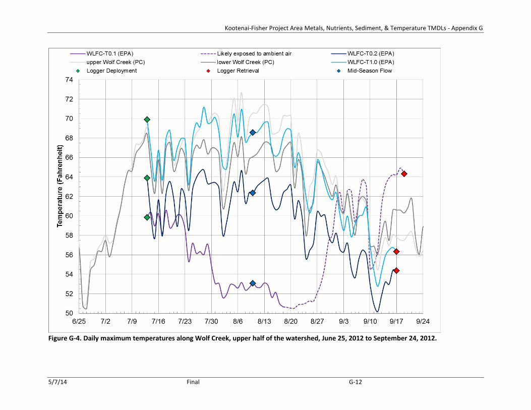
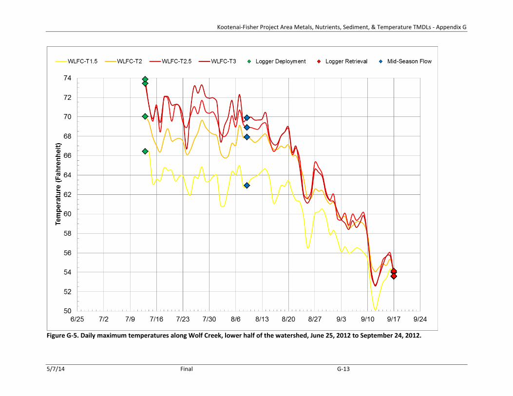
G2.5 TEMPERATURE DATA ANALYSIS Stream temperatures in Wolf Creek generally increase from its source downstream to its mouth (Figure G-3). Brush (BRSHC) and Richard (RCHDC) creeks, tributaries to Wolf Creek, contributed considerably cooler water while the highest temperatures were observed at the mouth of Little Wolf Creek (LWLFC). Maximum temperatures (Figure G-4, Figure G-5, and Figure G-6) generally follow similar patterns with temperatures steadily increasing downstream of the confluence with Brush Creek with coolest temperatures in the headwaters of Wolf Creek (WLFC-T0.1 and WLFC-T0.2), Brush Creek (BRSHC) and Richard Creek (RCHDC). Four temperature loggers (WLFC-T0.1, DRFKC, LWLFC, and CALXC) were observed to be either fully exposed to ambient air in dry channels or partially exposed and partially submerged in shallow wet
Kootenai-Fisher Project Area Metals, Nutrients, Sediment, & Temperature TMDLs - Appendix G
5/7/14 Final G-10
channels on August 9 or 10, 2012 and September 17 or 19, 2012. Therefore, the temperature data from each logger were evaluated and as described below, data from certain time periods were excluded from further analyses.
• Calx Creek: Daily maximum temperature increased 13° F between July 6 and 7, 2012. Maximum daily temperatures in the high 70s °F though lower 100s °F persisted until the logger was retrieved on September 17, 2012. During this time period, diurnal variation was considerably larger than the diurnal variation for loggers that remained fully submerged through the summer. Therefore, data collected between July 7 and September 17, 2012 were excluded from further analyses.
• Dry Fork Creek: Daily maximum temperatures increased 15° F between July 7 and 8, 2012. Maximum daily temperatures in the high 70s°F though the lower 90s°F were regularly monitored through July and August. Daily maximum temperatures decreased into the 60s°F in September; however, such temperatures were considerably warmer as compared to the loggers that were fully submerged in September. Additionally, from July 8 through September 17, 2012, diurnal variation was considerably larger than the diurnal variation for the loggers that remained fully submerged through the summer. Therefore, data collected between July 8 and September 17, 2012 were excluded from further analyses.
• Little Wolf Creek: Daily maximum temperatures began increasing considerably on August 27, 2012 and remained elevated through September 8, 2012. From August 28 through September 8, 2012, daily maximum temperatures were in the 90s° F and were 25° F warmer than any other logger that remained fully submerged throughout the summer. Diurnal variation was consistently in excess of 40° F during this time period. Temperatures rapidly fell on September 8 and 9, 2012 and appeared to remain consistent with submerged loggers until this logger was retrieved on September 17, 2012. Therefore, data collected between August 27 and September 8, 2012 were excluded from further analyses.
• Wolf Creek (RM 0.1): The daily variations between daily maximum temperatures from August 18 through September 19, 2012 were inconsistent with such variation for the other loggers on Wolf Creek. From August 18 through August 25, 2012, the variations between one-half hourly measurements were inconsistent with such variations from earlier in the summer and were inconsistent with such variations from other loggers in Wolf Creek. During this time period, temperatures would vary a few tenths of a degree between measurements at other loggers while temperatures at this logger remained constant or nearly constant for many hours at a time. On August 26, 2012, temperatures began to increase and daily maximum temperatures continued to increase and remain elevated (as compared to daily maximums earlier in the summer when this logger was submerged) until retrieval on September 19, 2012. Therefore, data collected between September 1 and 19, 2012 were excluded from further analyses.

Kootenai-Fisher Project Area Metals, Nutrients, Sediment, & Temperature TMDLs - Appendix G
5/7/14 Final G-11
Note: Elevated temperature data, that likely represent periods when the loggers were exposed to ambient air, were excluded from this figure. Figure G-3. Box-and-whisker plots of DEQ temperature data, June 26 or July13 to September 17 or 19, 2012.
Kootenai-Fisher Project Area Metals, Nutrients, Sediment, & Temperature TMDLs - Appendix G
5/7/14 Final G-12
Figure G-4. Daily maximum temperatures along Wolf Creek, upper half of the watershed, June 25, 2012 to September 24, 2012.
Kootenai-Fisher Project Area Metals, Nutrients, Sediment, & Temperature TMDLs - Appendix G
5/7/14 Final G-13
Figure G-5. Daily maximum temperatures along Wolf Creek, lower half of the watershed, June 25, 2012 to September 24, 2012.

Kootenai-Fisher Project Area Metals, Nutrients, Sediment, & Temperature TMDLs - Appendix G
5/7/14 Final G-14
Figure G-6. Daily maximum temperatures on the tributaries to Wolf Creek, June 25, 2012 to September 24, 2012.
Kootenai-Fisher Project Area Metals, Nutrients, Sediment, & Temperature TMDLs - Appendix G
5/7/14 Final G-15
G3.0 QUAL2K MODEL DEVELOPMENT A QUAL2K model was used to simulate temperatures in Wolf Creek. QUAL2K is supported by EPA and has been used extensively for TMDL development and point source permitting across the country. The QUAL2K model is suitable for simulating hydraulics and water quality conditions of small rivers and creeks. It is a one-dimensional uniform flow model with the assumption of a completely mixed system for each computational cell. QUAL2K assumes that the major pollutant transport mechanisms, advection and dispersion, are significant only along the longitudinal direction of flow. The heat budget and temperature are simulated as a function of meteorology on a daily time scale. Heat and mass inputs through point and nonpoint sources are also simulated. The model allows for multiple waste discharges, water withdrawals, nonpoint source loading, tributary flows, and incremental inflows and outflows. QUAL2K simulates instream temperatures via a heat balance that accounts “for heat transfers from adjacent elements, loads, withdrawals, the atmosphere, and the sediments” (Chapra et al., 2007, p. 19). The most current release of QUAL2K was used (version 2.11b8, January 2009). The model is publicly available at http://www.epa.gov/athens/wwqtsc/html/QUAL2K.html. Additional information regarding QUAL2K is presented in the Quality Assurance Project Plan for Montana TMDL Support: Temperature Modeling (Tetra Tech, Inc., 2012). The following describes the process that was used to setup, calibrate, and validate the QUAL2K model for Wolf Creek.
G3.1 MODEL FRAMEWORK The modeling domain included the area just near the confluence with Weigel Creek down to the confluence with the Fisher River (Figure G-2). Channel geometry and stream temperature, flow, and shade data were collected in 2012 to support the QUAL2K model for the Wolf Creek. Data are summarized within this appendix; raw data may be obtained by contacting DEQ’s Water Quality Planning Bureau.
G3.2 MODEL CONFIGURATION AND SETUP Model configuration involved setting up the model computational grid and setting initial conditions, boundary conditions, and hydraulic and light and heat parameters. All inputs were longitudinally referenced, allowing spatial and continuous inputs to apply to certain zones or specific stream segments. This section describes the configuration and key components of the model. G3.2.1 Modeling Time Period The calibration period input parameters were based upon August 9, 2012; flow was monitored August 9 or 10, 2012 at all EPA logger sites on Wolf Creek and its major tributaries. Since flow was monitored at more sites on Wolf Creek on August 9, 2012, this date was selected for calibration. Dry channels were observed during August 9, 2012 at the logger sites on Calx Creek and Dry Fork Creek. The validation period input parameters were based upon September 16, 2012, which is just before the retrieval of all the EPA loggers. EPA loggers were retrieved on September 17 and 19, 2012. The last full day of temperature data for all EPA loggers was September 16, 2012. Plum Creek loggers were deployed until October 2, 2012 and have full temperature records for September 16, 2012. Flow data monitored on September 17, 2012 was assumed to be representative of flow conditions on September 16, 2012.
Kootenai-Fisher Project Area Metals, Nutrients, Sediment, & Temperature TMDLs - Appendix G
5/7/14 Final G-16
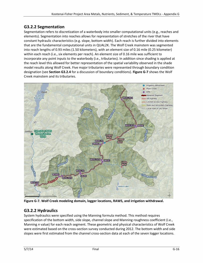
G3.2.2 Segmentation Segmentation refers to discretization of a waterbody into smaller computational units (e.g., reaches and elements). Segmentation into reaches allows for representation of stretches of the river that have constant hydraulic characteristics (e.g. slope, bottom width). Each reach is further divided into elements that are the fundamental computational units in QUAL2K. The Wolf Creek mainstem was segmented into reach lengths of 0.93 miles (1.50 kilometers), with an element size of 0.16 mile (0.25 kilometer) within each reach (i.e., six elements per reach). An element size of 0.16 mile was sufficient to incorporate any point inputs to the waterbody (i.e., tributaries). In addition since shading is applied at the reach level this allowed for better representation of the spatial variability observed in the shade model results along Wolf Creek. Five major tributaries were represented through boundary condition designation (see Section G3.2.4 for a discussion of boundary conditions). Figure G-7 shows the Wolf Creek mainstem and its tributaries.
Figure G-7. Wolf Creek modeling domain, logger locations, RAWS, and irrigation withdrawal. G3.2.2 Hydraulics System hydraulics were specified using the Manning formula method. This method requires specification of the bottom width, side slope, channel slope and Manning roughness coefficient (i.e., Manning n value) for each reach segment. These geometric and physical characteristics of Wolf Creek were estimated based on the cross-section survey conducted during 2012. The bottom width and side slopes were first estimated from the channel cross-section data at each of the seven logger locations.
Kootenai-Fisher Project Area Metals, Nutrients, Sediment, & Temperature TMDLs - Appendix G
5/7/14 Final G-17
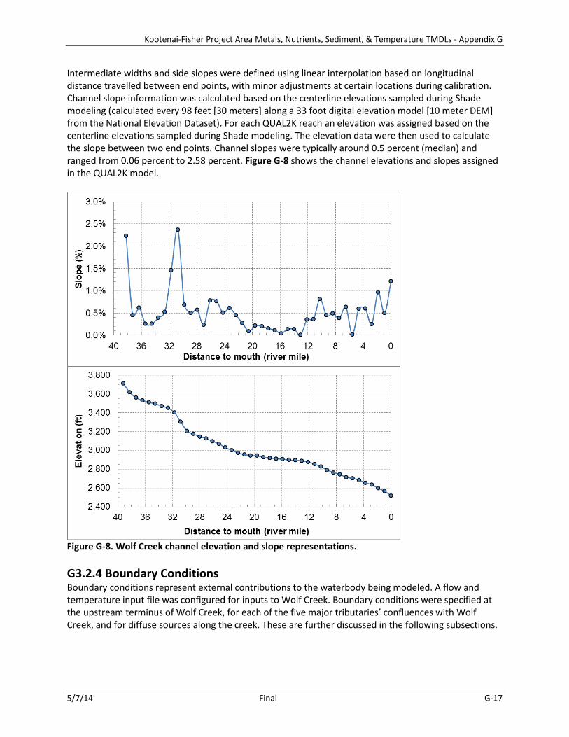
Intermediate widths and side slopes were defined using linear interpolation based on longitudinal distance travelled between end points, with minor adjustments at certain locations during calibration. Channel slope information was calculated based on the centerline elevations sampled during Shade modeling (calculated every 98 feet [30 meters] along a 33 foot digital elevation model [10 meter DEM] from the National Elevation Dataset). For each QUAL2K reach an elevation was assigned based on the centerline elevations sampled during Shade modeling. The elevation data were then used to calculate the slope between two end points. Channel slopes were typically around 0.5 percent (median) and ranged from 0.06 percent to 2.58 percent. Figure G-8 shows the channel elevations and slopes assigned in the QUAL2K model.
Figure G-8. Wolf Creek channel elevation and slope representations. G3.2.4 Boundary Conditions Boundary conditions represent external contributions to the waterbody being modeled. A flow and temperature input file was configured for inputs to Wolf Creek. Boundary conditions were specified at the upstream terminus of Wolf Creek, for each of the five major tributaries’ confluences with Wolf Creek, and for diffuse sources along the creek. These are further discussed in the following subsections.
Kootenai-Fisher Project Area Metals, Nutrients, Sediment, & Temperature TMDLs - Appendix G
5/7/14 Final G-18
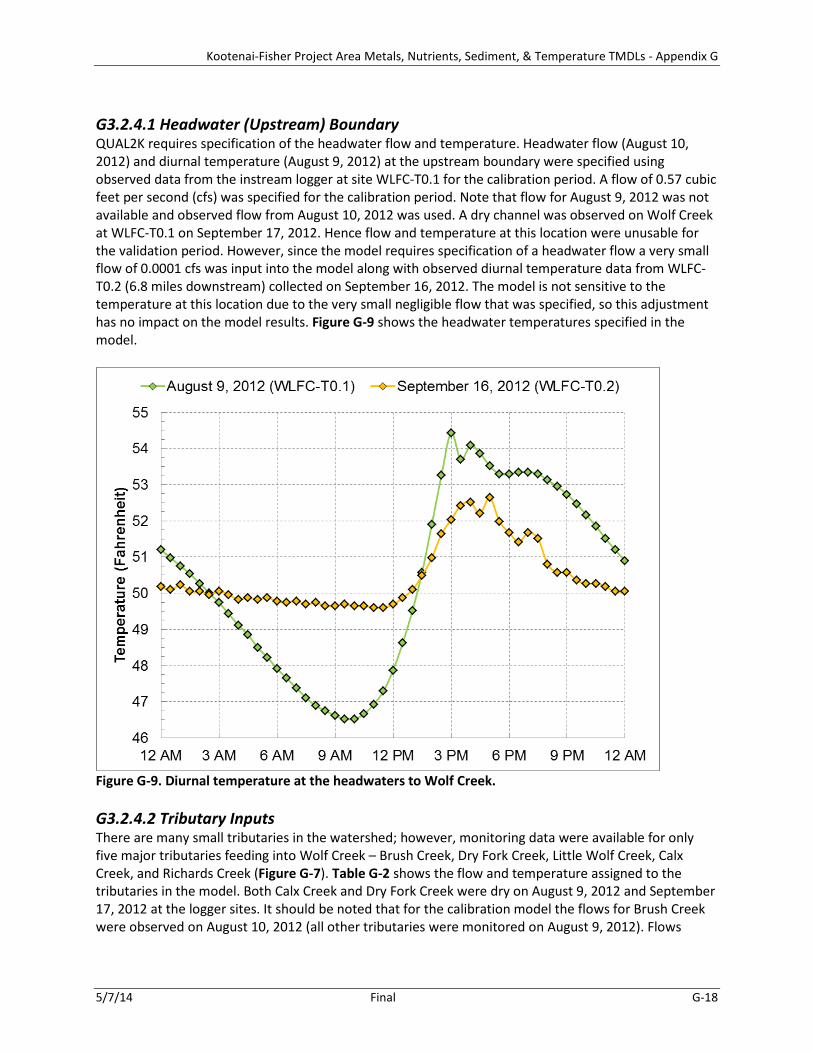
G3.2.4.1 Headwater (Upstream) Boundary QUAL2K requires specification of the headwater flow and temperature. Headwater flow (August 10, 2012) and diurnal temperature (August 9, 2012) at the upstream boundary were specified using observed data from the instream logger at site WLFC-T0.1 for the calibration period. A flow of 0.57 cubic feet per second (cfs) was specified for the calibration period. Note that flow for August 9, 2012 was not available and observed flow from August 10, 2012 was used. A dry channel was observed on Wolf Creek at WLFC-T0.1 on September 17, 2012. Hence flow and temperature at this location were unusable for the validation period. However, since the model requires specification of a headwater flow a very small flow of 0.0001 cfs was input into the model along with observed diurnal temperature data from WLFC-T0.2 (6.8 miles downstream) collected on September 16, 2012. The model is not sensitive to the temperature at this location due to the very small negligible flow that was specified, so this adjustment has no impact on the model results. Figure G-9 shows the headwater temperatures specified in the model.
Figure G-9. Diurnal temperature at the headwaters to Wolf Creek. G3.2.4.2 Tributary Inputs There are many small tributaries in the watershed; however, monitoring data were available for only five major tributaries feeding into Wolf Creek – Brush Creek, Dry Fork Creek, Little Wolf Creek, Calx Creek, and Richards Creek (Figure G-7). Table G-2 shows the flow and temperature assigned to the tributaries in the model. Both Calx Creek and Dry Fork Creek were dry on August 9, 2012 and September 17, 2012 at the logger sites. It should be noted that for the calibration model the flows for Brush Creek were observed on August 10, 2012 (all other tributaries were monitored on August 9, 2012). Flows
Kootenai-Fisher Project Area Metals, Nutrients, Sediment, & Temperature TMDLs - Appendix G
5/7/14 Final G-19
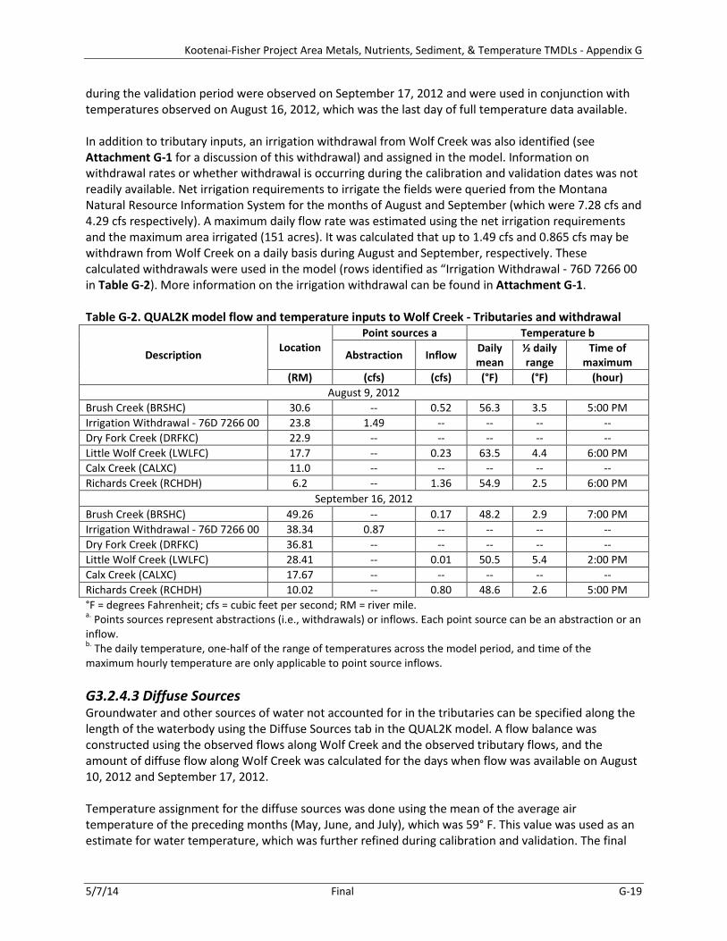
during the validation period were observed on September 17, 2012 and were used in conjunction with temperatures observed on August 16, 2012, which was the last day of full temperature data available. In addition to tributary inputs, an irrigation withdrawal from Wolf Creek was also identified (see Attachment G-1 for a discussion of this withdrawal) and assigned in the model. Information on withdrawal rates or whether withdrawal is occurring during the calibration and validation dates was not readily available. Net irrigation requirements to irrigate the fields were queried from the Montana Natural Resource Information System for the months of August and September (which were 7.28 cfs and 4.29 cfs respectively). A maximum daily flow rate was estimated using the net irrigation requirements and the maximum area irrigated (151 acres). It was calculated that up to 1.49 cfs and 0.865 cfs may be withdrawn from Wolf Creek on a daily basis during August and September, respectively. These calculated withdrawals were used in the model (rows identified as “Irrigation Withdrawal - 76D 7266 00 in Table G-2). More information on the irrigation withdrawal can be found in Attachment G-1. Table G-2. QUAL2K model flow and temperature inputs to Wolf Creek - Tributaries and withdrawal
Description Location
Point sources a Temperature b
Abstraction Inflow Daily mean
½ daily range
Time of maximum
(RM) (cfs) (cfs) (°F) (°F) (hour) August 9, 2012
Brush Creek (BRSHC) 30.6 -- 0.52 56.3 3.5 5:00 PM Irrigation Withdrawal - 76D 7266 00 23.8 1.49 -- -- -- -- Dry Fork Creek (DRFKC) 22.9 -- -- -- -- -- Little Wolf Creek (LWLFC) 17.7 -- 0.23 63.5 4.4 6:00 PM Calx Creek (CALXC) 11.0 -- -- -- -- -- Richards Creek (RCHDH) 6.2 -- 1.36 54.9 2.5 6:00 PM
September 16, 2012 Brush Creek (BRSHC) 49.26 -- 0.17 48.2 2.9 7:00 PM Irrigation Withdrawal - 76D 7266 00 38.34 0.87 -- -- -- -- Dry Fork Creek (DRFKC) 36.81 -- -- -- -- -- Little Wolf Creek (LWLFC) 28.41 -- 0.01 50.5 5.4 2:00 PM Calx Creek (CALXC) 17.67 -- -- -- -- -- Richards Creek (RCHDH) 10.02 -- 0.80 48.6 2.6 5:00 PM °F = degrees Fahrenheit; cfs = cubic feet per second; RM = river mile. a. Points sources represent abstractions (i.e., withdrawals) or inflows. Each point source can be an abstraction or an inflow. b. The daily temperature, one-half of the range of temperatures across the model period, and time of the maximum hourly temperature are only applicable to point source inflows. G3.2.4.3 Diffuse Sources Groundwater and other sources of water not accounted for in the tributaries can be specified along the length of the waterbody using the Diffuse Sources tab in the QUAL2K model. A flow balance was constructed using the observed flows along Wolf Creek and the observed tributary flows, and the amount of diffuse flow along Wolf Creek was calculated for the days when flow was available on August 10, 2012 and September 17, 2012. Temperature assignment for the diffuse sources was done using the mean of the average air temperature of the preceding months (May, June, and July), which was 59° F. This value was used as an estimate for water temperature, which was further refined during calibration and validation. The final

Kootenai-Fisher Project Area Metals, Nutrients, Sediment, & Temperature TMDLs - Appendix G
5/7/14 Final G-20
diffuse source water temperatures were kept the same for the calibration and validation period. The final flow and water temperature assignments are shown Table G-3. Table G-3. QUAL2K model flow and temperature inputs to Wolf Creek - Diffuse sources
Description Location a Diffuse
Abstraction Diffuse Inflow
Upstream Downstream Inflow Temp (RM) (RM) (cfs) (cfs) (°F)
August 9, 2012 From WLFC-0.1 to WLFC-0.2 37.8 30.6 -- 3.86 57.2 From WLFC-0.2 to WLFC-T1 30.6 22.9 -- 1.95 57.2 From WLFC-T1 to WLFC-T1.5 22.9 17.7 -- 9.23 57.2 From WLFC-T1.5 to WLFC-T2 17.7 11.0 -- <0.01 57.2 From WLFC-T2 to WLFC-T2.5 11.0 6.2 -- 3.28 57.2 From WLFC-T2.5 to WLFC-T3 6.2 0.0 -- 0.67 57.2
September 16, 2012 From WLFC-0.1 to WLFC-0.2 37.8 30.6 -- 2.48 57.2 From WLFC-0.2 to WLFC-T1 30.6 22.9 -- 0.34 57.2 From WLFC-T1 to WLFC-T1.5 22.9 17.7 -- 5.14 57.2 From WLFC-T1.5 to WLFC-T2 17.7 11.0 -- 0.08 57.2 From WLFC-T2 to WLFC-T2.5 11.0 6.2 -- 0.55 57.2 From WLFC-T2.5 to WLFC-T3 6.2 0.0 -- 1.00 57.2 °F = degrees Fahrenheit; cfs = cubic feet per second; RM = river mile. a. Upstream and downstream termini of segment G3.2.5 Meteorological Data The surface boundary conditions are determined by the meteorological conditions in QUAL2K. The QUAL2K model requires hourly meteorological input for the following parameters: air temperature, dew point temperature, wind speed, and cloud cover. There are two weather stations in the vicinity of the Wolf Creek watershed – Fisher River RAWS (TS259) and Hand Creek Weather Station (USS0014A14S). The Fisher River RAWS (Figure G-7) records hourly air temperature, dew point temperature, wind speed and solar radiation, whereas the Hand Creek weather station only records hourly air temperature data. The Fisher River RAWS hourly observed meteorological data were used to develop the QUAL2K model after appropriate unit conversions. The wind speed measurements at the Fisher River RAWS were measured at 20 feet (6.1 meters) above the ground. QUAL2K requires that the wind speed be at a height of 23 feet (7.0 meters). The wind speed measurements (Uw,z in meters/second) taken at a height of 6.1 meters (zw in meters) were converted to equivalent conditions at a height of z = 7.0 meters (the appropriate height for input to the evaporative heat loss equation), using the exponential wind law equation suggested in the QUAL2K user’s manual:
15.0
=
wwzw z
zUU
G3.2.6 Shade Data The QUAL2K model allows for spatial and temporal specification of shade, which is the fraction of potential solar radiation that is blocked by topography and vegetation. A shade model was developed and calibrated for the Wolf Creek. The calibrated shade model was first run to simulate hourly shade estimates for August 9, 2012 and September 16, 2012 every 98 feet (i.e., 30 meters, the resolution of

Kootenai-Fisher Project Area Metals, Nutrients, Sediment, & Temperature TMDLs - Appendix G
5/7/14 Final G-21
the shade model) along Wolf Creek. Reach-averaged integrated hourly effective shade results were then computed at every 0.93 miles (1.5 kilometer) using the macro in the Shade model located under the “Diel Shade QUAL2K” worksheet. The reach-averaged results were then input into each reach within the QUAL2K model. The overall average shade on September 16, 2012 (71.7%) was greater than that predicted on August 9, 2012 (60.7%). A more detailed discussion on the shade modeling can be found under Attachment G-1.
G3.3 MODEL EVALUATION CRITERIA The goodness of fit for the simulated temperature using the QUAL2K model was summarized using the absolute mean error (AME) and relative error (REL) as a measure of the deviation of model-predicted temperature values (P) from the measured, observed values (O). These model performance measures were calculated as follows:
∑=
−=n
nnn OP
NAME
1
1
∑∑
=
=−
= n
n n
n
n nn
O
OPREL
1
1
These performance measures are detailed in the following section relative to model calibration and validation.
G3.4 MODEL CALIBRATION AND VALIDATION The time periods selected for calibration and validation were August 9, 2012 and September 16, 2012, respectively. These dates were selected as they had the most comprehensive dataset available for modeling and corresponded to the synoptic study done for Wolf Creek, which included collecting flow, temperature, shade, and channel geometry information. Flow, depth, velocity and temperature data were available at eight locations along the mainstem of Wolf Creek. Table G-4 shows the monitoring sites used for calibration and validation. Data from both available sources, EPA and Plum Creek Timber Company, were used. Table G-4. Temperature calibration and validation locations
Site name Distance (RM) Available Data Source WLFC-T0.2 30.9 Flow, depth, velocity, and temperature EPA Upper Wolf 26.7 Temperature Plum Creek Timber Company Lower Wolf 25.0 Temperature Plum Creek Timber Company WLFC-T1 23.5 Flow, depth, velocity, and temperature EPA WLFC-T1.5 18.0 Flow, depth, velocity, and temperature EPA WLFC-T2 11.1 Flow, depth, velocity, and temperature EPA WLFC-T2.5 6.9 Flow, depth, velocity, and temperature EPA WLFC-T3 0.7 Flow, depth, velocity, and temperature EPA The first step for calibration was adjusting the flow balance and calibrating the system hydraulics. A flow balance was first constructed for the calibration and validation dates. This involved accounting for all the
Kootenai-Fisher Project Area Metals, Nutrients, Sediment, & Temperature TMDLs - Appendix G
5/7/14 Final G-22
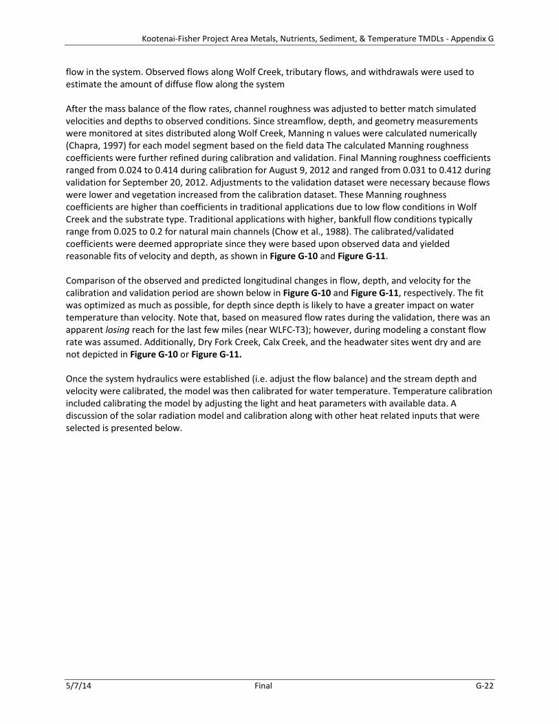
flow in the system. Observed flows along Wolf Creek, tributary flows, and withdrawals were used to estimate the amount of diffuse flow along the system After the mass balance of the flow rates, channel roughness was adjusted to better match simulated velocities and depths to observed conditions. Since streamflow, depth, and geometry measurements were monitored at sites distributed along Wolf Creek, Manning n values were calculated numerically (Chapra, 1997) for each model segment based on the field data The calculated Manning roughness coefficients were further refined during calibration and validation. Final Manning roughness coefficients ranged from 0.024 to 0.414 during calibration for August 9, 2012 and ranged from 0.031 to 0.412 during validation for September 20, 2012. Adjustments to the validation dataset were necessary because flows were lower and vegetation increased from the calibration dataset. These Manning roughness coefficients are higher than coefficients in traditional applications due to low flow conditions in Wolf Creek and the substrate type. Traditional applications with higher, bankfull flow conditions typically range from 0.025 to 0.2 for natural main channels (Chow et al., 1988). The calibrated/validated coefficients were deemed appropriate since they were based upon observed data and yielded reasonable fits of velocity and depth, as shown in Figure G-10 and Figure G-11. Comparison of the observed and predicted longitudinal changes in flow, depth, and velocity for the calibration and validation period are shown below in Figure G-10 and Figure G-11, respectively. The fit was optimized as much as possible, for depth since depth is likely to have a greater impact on water temperature than velocity. Note that, based on measured flow rates during the validation, there was an apparent losing reach for the last few miles (near WLFC-T3); however, during modeling a constant flow rate was assumed. Additionally, Dry Fork Creek, Calx Creek, and the headwater sites went dry and are not depicted in Figure G-10 or Figure G-11. Once the system hydraulics were established (i.e. adjust the flow balance) and the stream depth and velocity were calibrated, the model was then calibrated for water temperature. Temperature calibration included calibrating the model by adjusting the light and heat parameters with available data. A discussion of the solar radiation model and calibration along with other heat related inputs that were selected is presented below.
Kootenai-Fisher Project Area Metals, Nutrients, Sediment, & Temperature TMDLs - Appendix G
5/7/14 Final G-23
(a)
(b)
(c) Figure G-10. Observed and predicted flow (Q), velocity (U), and depth (H) on August 9, 2012 (calibration).

Kootenai-Fisher Project Area Metals, Nutrients, Sediment, & Temperature TMDLs - Appendix G
5/7/14 Final G-24
(a)
(b)
(c) Figure G-11. Observed and predicted flow (Q), velocity (U), and depth (H) on September 16, 2012 (validation).
Kootenai-Fisher Project Area Metals, Nutrients, Sediment, & Temperature TMDLs - Appendix G
5/7/14 Final G-25
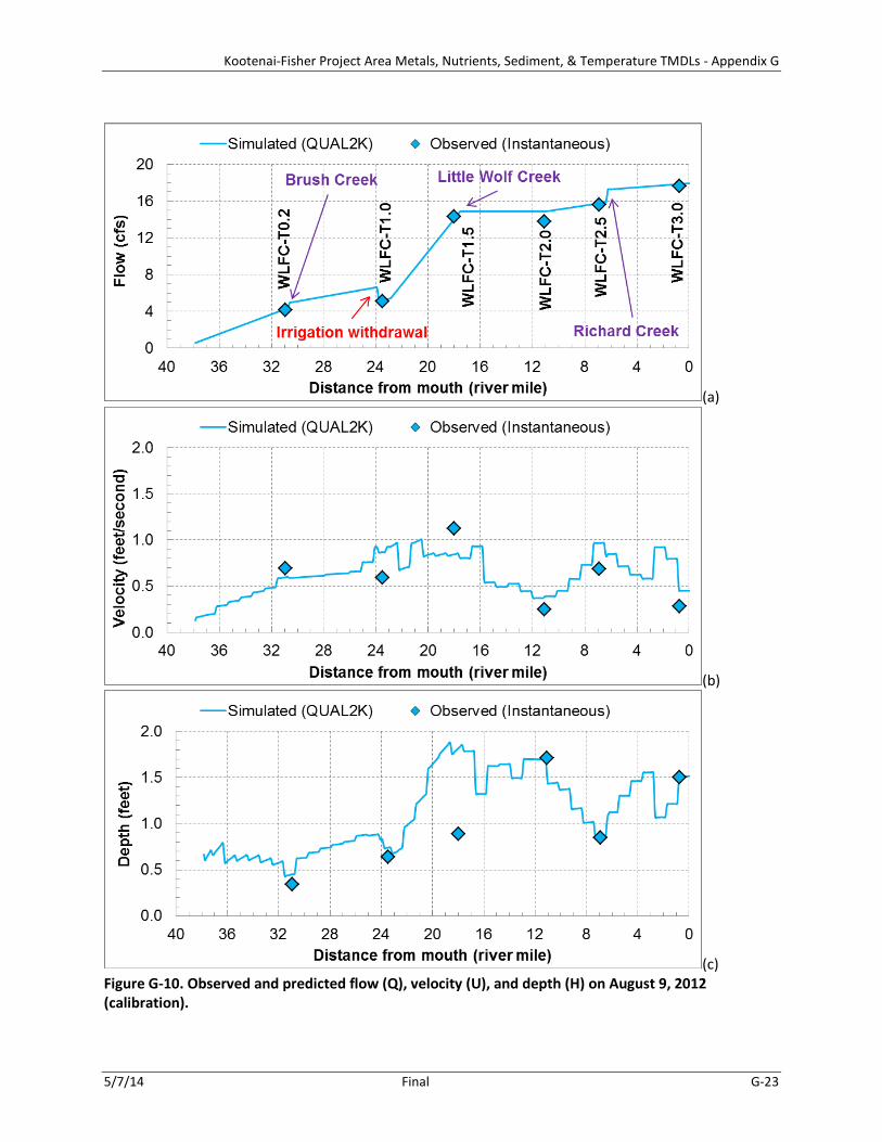
Hourly solar radiation is an important factor that affects stream temperature. The QUAL2K model does not allow for input of solar radiation measurements. Instead the model calculates short wave solar radiation using an atmospheric attenuation model. For the Wolf Creek QUAL2K model, the Ryan-Stolzenbach model was used to calculate the solar radiation. The calculated solar radiation values (without stream shade) for the calibration and validation date were compared with observed solar radiation measurements at the Fisher Creek RAWS. Figure G-12 shows the observed and predicted solar radiation for the calibration and validation. No cloud cover data were available and the observed solar radiation during calibration showed some influence due to cloud cover especially during hour 15. The cloud cover was adjusted to more closely mimic observed solar radiation during calibration on August 9, 2012. A cloud cover specification of 75 percent at hour 15 and a 40 percent cloud cover adjustment at all other times during the day was specified to match the observed solar radiation on the calibration day. No adjustment was required to be made to the cloud cover during the validation period on September 16, 2012. The Ryan-Stolzenbach atmospheric transmission coefficient was set at 0.8 for the calibration and validation dates.
(a)
(b) Figure G-12. Observed and predicted solar radiation on August 9, 2012 and September 16, 2012 (calibration and validation).
Kootenai-Fisher Project Area Metals, Nutrients, Sediment, & Temperature TMDLs - Appendix G
5/7/14 Final G-26
The longwave solar radiation model and the evaporation and air conduction/convections models were kept at the default QUAL2K settings. The solar radiation settings are shown in Table G-5. Table G-5. Solar radiation settings
Parameter Value Solar shortwave radiation model Atmospheric attenuation model for solar Ryan-Stolzenbach Ryan-Stolzenbach solar parameter -- atmospheric transmission coefficient (0.70-0.91, default 0.8) 0.8
Downwelling atmospheric longwave infrared radiation Atmospheric longwave emissivity model Brunt
Evaporation and air convection/conduction Wind speed function for evaporation and air convection/conduction Brady-Graves-Geyer The sediment heat parameters were also evaluated for calibration. These parameters have an impact especially on the minimum temperatures simulated. In particular the sediment thermal thickness, sediment thermal diffusivity, and sediment heat capacity were adjusted during calibration. The sediment thermal thickness was slightly increased from the default value of 10 cm to 15 cm, and the sediment heat capacity of all component materials of the stream was also increased to 0.55 calories per gram °C from the default value of 0.432 calories per gram °C. The sediment thermal diffusivity was set to a value of 0.0118 square centimeters per second (Chapra et al., 2007). This was consistent with the stream photos that indicated a predominant rocky substrate along the main channel. These adjustments helped in improving the minimum temperatures simulated. Calibration was followed by validation. The validation provides a test of the calibrated model parameters under a different set of conditions. Only those variables that changed with time were changed during validation to confirm the hydraulic variables. Variables that changed with time included headwater and tributary instream temperatures, air and dew point temperatures, wind speed, cloud cover, solar radiation, and shade. Reach properties such as slope, width, and other associated parameters were unchanged from the calibration. Stream depth and velocities varied greatly during September and the Manning roughness coefficients were varied to reflect these conditions (this is further discussed in Section G3.2.3). All other inputs were based on observed data in September 16, 2012. Groundwater temperatures, for which there were no direct observed data, were unchanged since they are not expected to change significantly between August 9 and September 16. Figure G-13 and Figure F-14 show the calibration and validation results along Wolf Creek. As can be seen in the figures, the ranges of temperatures during calibration and validation are quite different. In addition, the observed temperatures during the calibration are much warmer than those during the validation and can be as high as 6° C warmer. The temperature calibration and validation statistics of the average, maximum, and minimum temperatures are shown in Table G-6 and Table G-7, respectively.
Kootenai-Fisher Project Area Metals, Nutrients, Sediment, & Temperature TMDLs - Appendix G
5/7/14 Final G-27
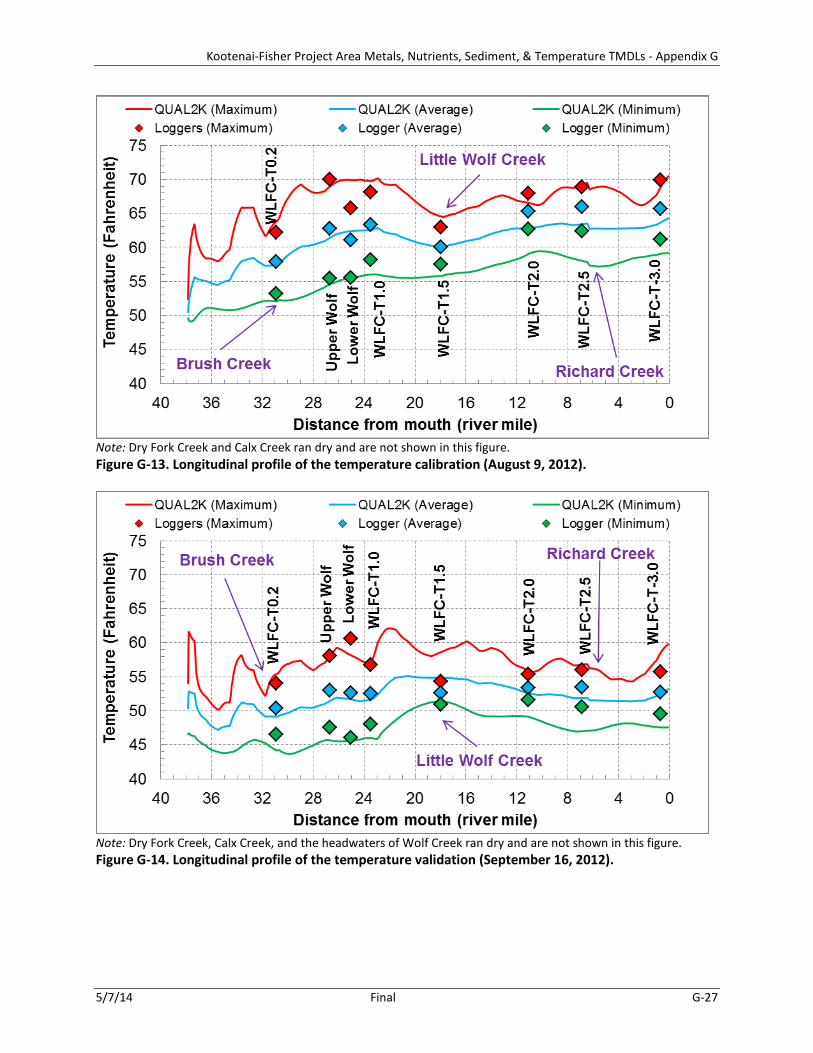
Note: Dry Fork Creek and Calx Creek ran dry and are not shown in this figure. Figure G-13. Longitudinal profile of the temperature calibration (August 9, 2012).
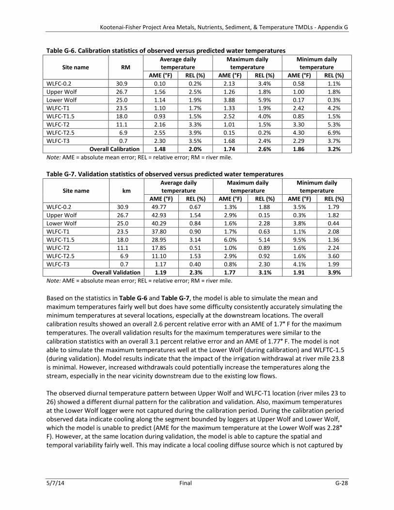
Note: Dry Fork Creek, Calx Creek, and the headwaters of Wolf Creek ran dry and are not shown in this figure. Figure G-14. Longitudinal profile of the temperature validation (September 16, 2012).
Kootenai-Fisher Project Area Metals, Nutrients, Sediment, & Temperature TMDLs - Appendix G
5/7/14 Final G-28
Table G-6. Calibration statistics of observed versus predicted water temperatures
Site name RM Average daily temperature
Maximum daily temperature
Minimum daily temperature
AME (°F) REL (%) AME (°F) REL (%) AME (°F) REL (%) WLFC-0.2 30.9 0.10 0.2% 2.13 3.4% 0.58 1.1% Upper Wolf 26.7 1.56 2.5% 1.26 1.8% 1.00 1.8% Lower Wolf 25.0 1.14 1.9% 3.88 5.9% 0.17 0.3% WLFC-T1 23.5 1.10 1.7% 1.33 1.9% 2.42 4.2% WLFC-T1.5 18.0 0.93 1.5% 2.52 4.0% 0.85 1.5% WLFC-T2 11.1 2.16 3.3% 1.01 1.5% 3.30 5.3% WLFC-T2.5 6.9 2.55 3.9% 0.15 0.2% 4.30 6.9% WLFC-T3 0.7 2.30 3.5% 1.68 2.4% 2.29 3.7%
Overall Calibration 1.48 2.0% 1.74 2.6% 1.86 3.2% Note: AME = absolute mean error; REL = relative error; RM = river mile. Table G-7. Validation statistics of observed versus predicted water temperatures
Site name km Average daily temperature
Maximum daily temperature
Minimum daily temperature
AME (°F) REL (%) AME (°F) REL (%) AME (°F) REL (%) WLFC-0.2 30.9 49.77 0.67 1.3% 1.88 3.5% 1.79 Upper Wolf 26.7 42.93 1.54 2.9% 0.15 0.3% 1.82 Lower Wolf 25.0 40.29 0.84 1.6% 2.28 3.8% 0.44 WLFC-T1 23.5 37.80 0.90 1.7% 0.63 1.1% 2.08 WLFC-T1.5 18.0 28.95 3.14 6.0% 5.14 9.5% 1.36 WLFC-T2 11.1 17.85 0.51 1.0% 0.89 1.6% 2.24 WLFC-T2.5 6.9 11.10 1.53 2.9% 0.92 1.6% 3.60 WLFC-T3 0.7 1.17 0.40 0.8% 2.30 4.1% 1.99
Overall Validation 1.19 2.3% 1.77 3.1% 1.91 3.9% Note: AME = absolute mean error; REL = relative error; RM = river mile. Based on the statistics in Table G-6 and Table G-7, the model is able to simulate the mean and maximum temperatures fairly well but does have some difficulty consistently accurately simulating the minimum temperatures at several locations, especially at the downstream locations. The overall calibration results showed an overall 2.6 percent relative error with an AME of 1.7° F for the maximum temperatures. The overall validation results for the maximum temperatures were similar to the calibration statistics with an overall 3.1 percent relative error and an AME of 1.77° F. The model is not able to simulate the maximum temperatures well at the Lower Wolf (during calibration) and WLFTC-1.5 (during validation). Model results indicate that the impact of the irrigation withdrawal at river mile 23.8 is minimal. However, increased withdrawals could potentially increase the temperatures along the stream, especially in the near vicinity downstream due to the existing low flows. The observed diurnal temperature pattern between Upper Wolf and WLFC-T1 location (river miles 23 to 26) showed a different diurnal pattern for the calibration and validation. Also, maximum temperatures at the Lower Wolf logger were not captured during the calibration period. During the calibration period observed data indicate cooling along the segment bounded by loggers at Upper Wolf and Lower Wolf, which the model is unable to predict (AME for the maximum temperature at the Lower Wolf was 2.28° F). However, at the same location during validation, the model is able to capture the spatial and temporal variability fairly well. This may indicate a local cooling diffuse source which is not captured by
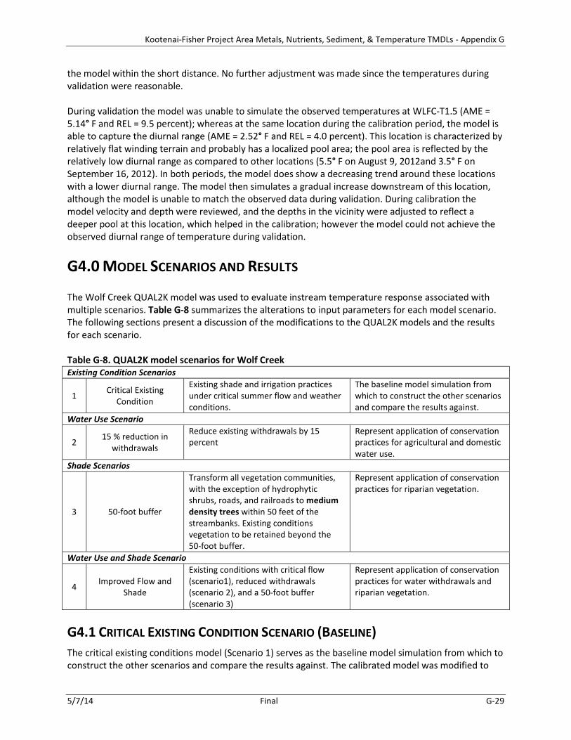
Kootenai-Fisher Project Area Metals, Nutrients, Sediment, & Temperature TMDLs - Appendix G
5/7/14 Final G-29
the model within the short distance. No further adjustment was made since the temperatures during validation were reasonable. During validation the model was unable to simulate the observed temperatures at WLFC-T1.5 (AME = 5.14° F and REL = 9.5 percent); whereas at the same location during the calibration period, the model is able to capture the diurnal range (AME = 2.52° F and REL = 4.0 percent). This location is characterized by relatively flat winding terrain and probably has a localized pool area; the pool area is reflected by the relatively low diurnal range as compared to other locations (5.5° F on August 9, 2012and 3.5° F on September 16, 2012). In both periods, the model does show a decreasing trend around these locations with a lower diurnal range. The model then simulates a gradual increase downstream of this location, although the model is unable to match the observed data during validation. During calibration the model velocity and depth were reviewed, and the depths in the vicinity were adjusted to reflect a deeper pool at this location, which helped in the calibration; however the model could not achieve the observed diurnal range of temperature during validation.
G4.0 MODEL SCENARIOS AND RESULTS
The Wolf Creek QUAL2K model was used to evaluate instream temperature response associated with multiple scenarios. Table G-8 summarizes the alterations to input parameters for each model scenario. The following sections present a discussion of the modifications to the QUAL2K models and the results for each scenario. Table G-8. QUAL2K model scenarios for Wolf Creek Existing Condition Scenarios
1 Critical Existing Condition
Existing shade and irrigation practices under critical summer flow and weather conditions.
The baseline model simulation from which to construct the other scenarios and compare the results against.
Water Use Scenario
2 15 % reduction in withdrawals
Reduce existing withdrawals by 15 percent
Represent application of conservation practices for agricultural and domestic water use.
Shade Scenarios
3 50-foot buffer
Transform all vegetation communities, with the exception of hydrophytic shrubs, roads, and railroads to medium density trees within 50 feet of the streambanks. Existing conditions vegetation to be retained beyond the 50-foot buffer.
Represent application of conservation practices for riparian vegetation.
Water Use and Shade Scenario
4 Improved Flow and Shade
Existing conditions with critical flow (scenario1), reduced withdrawals (scenario 2), and a 50-foot buffer (scenario 3)
Represent application of conservation practices for water withdrawals and riparian vegetation.
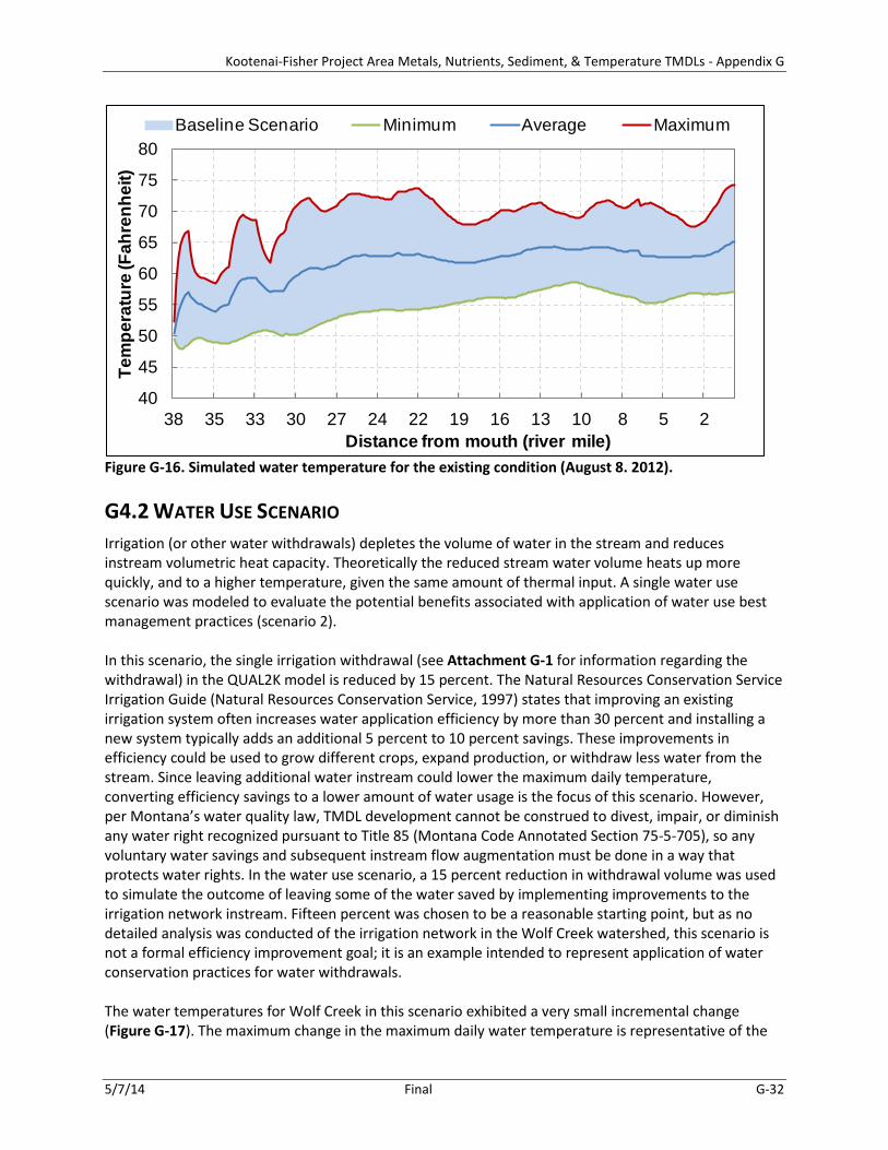
G4.1 CRITICAL EXISTING CONDITION SCENARIO (BASELINE) The critical existing conditions model (Scenario 1) serves as the baseline model simulation from which to construct the other scenarios and compare the results against. The calibrated model was modified to
Kootenai-Fisher Project Area Metals, Nutrients, Sediment, & Temperature TMDLs - Appendix G
5/7/14 Final G-30
represent critical flow and meteorological conditions. The critical low flow was set at the 25th percentile using the long-term discharge record from USGS gage 12302055 – Fisher River near Libby MT as a surrogate for Wolf Creek. The observed flow for August 9th (the calibration month and day) was extracted from the daily flow time series for each year from 1968 through 2012. The observed flow on August 9, 2012 (i.e. the calibration date) was estimated to be the 77th percentile flow across all the years (at 184 cfs). The 25th percentile flow value for August 9th across the entire flow time-period was estimated to be 102 cfs (45 percent less than the calibration period flow). The flows in Wolf Creek (headwaters, tributaries and diffuse sources) were adjusted by reducing them by 45 percent to achieve the critical 25th percentile flow condition in Wolf Creek. Meteorological conditions were established by calculating a critical meteorological condition using historical data from the Fisher River RAWS (TS259). These changes included adjusting the air temperature; dew point temperatures, wind speed, and cloud cover to represent critical conditions. The Fisher River RAWS has hourly data available for the period from July 27, 2004 to August 7, 2013. Since the weather data extends only for a period of eight years, a nearby station with long-term meteorological data (Kalispell Glacier Park International Airport [1988-2012]) was queried to confirm if the period from 2004 to 2013 were not anomalously warm or cold years and were similar to the overall historical normal. The monthly median and maximum air temperatures for the period from 2004 to 2012 were estimated to be similar to the overall period from 1988 through 2012, indicating that the period from 2004 through 2012 were not anomalous years (Figure G-15).
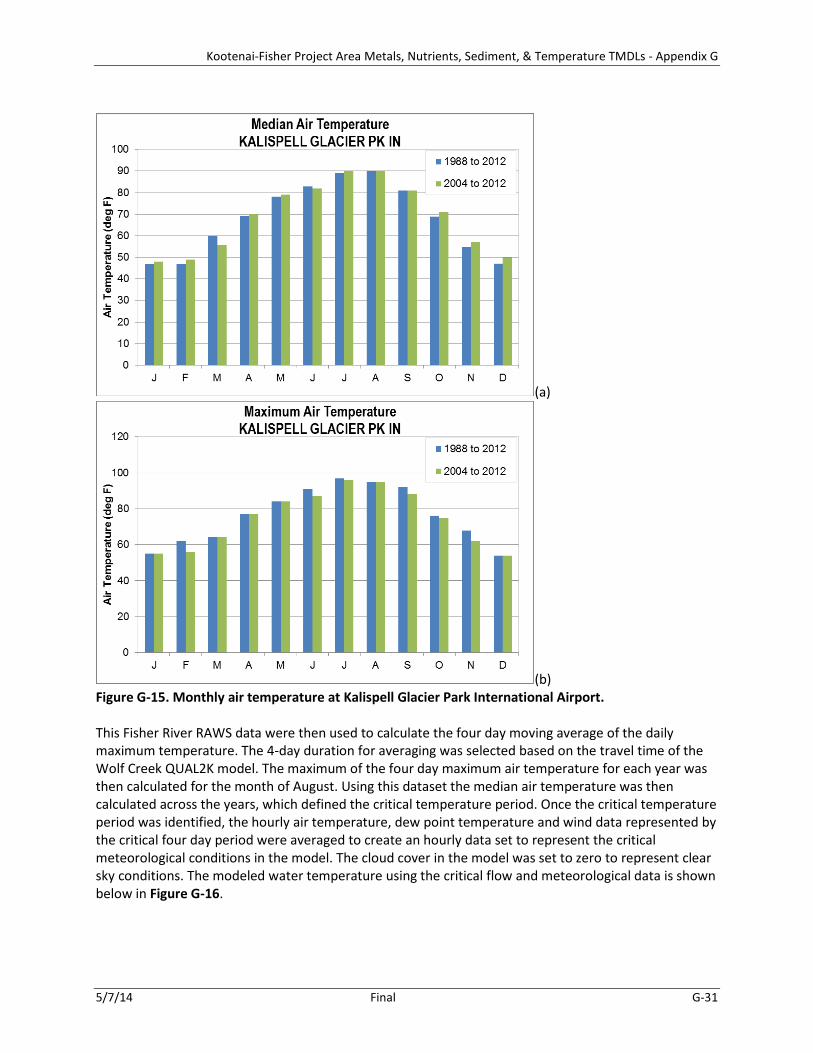
Kootenai-Fisher Project Area Metals, Nutrients, Sediment, & Temperature TMDLs - Appendix G
5/7/14 Final G-31
(a)
(b) Figure G-15. Monthly air temperature at Kalispell Glacier Park International Airport. This Fisher River RAWS data were then used to calculate the four day moving average of the daily maximum temperature. The 4-day duration for averaging was selected based on the travel time of the Wolf Creek QUAL2K model. The maximum of the four day maximum air temperature for each year was then calculated for the month of August. Using this dataset the median air temperature was then calculated across the years, which defined the critical temperature period. Once the critical temperature period was identified, the hourly air temperature, dew point temperature and wind data represented by the critical four day period were averaged to create an hourly data set to represent the critical meteorological conditions in the model. The cloud cover in the model was set to zero to represent clear sky conditions. The modeled water temperature using the critical flow and meteorological data is shown below in Figure G-16.
Kootenai-Fisher Project Area Metals, Nutrients, Sediment, & Temperature TMDLs - Appendix G
5/7/14 Final G-32
Figure G-16. Simulated water temperature for the existing condition (August 8. 2012).
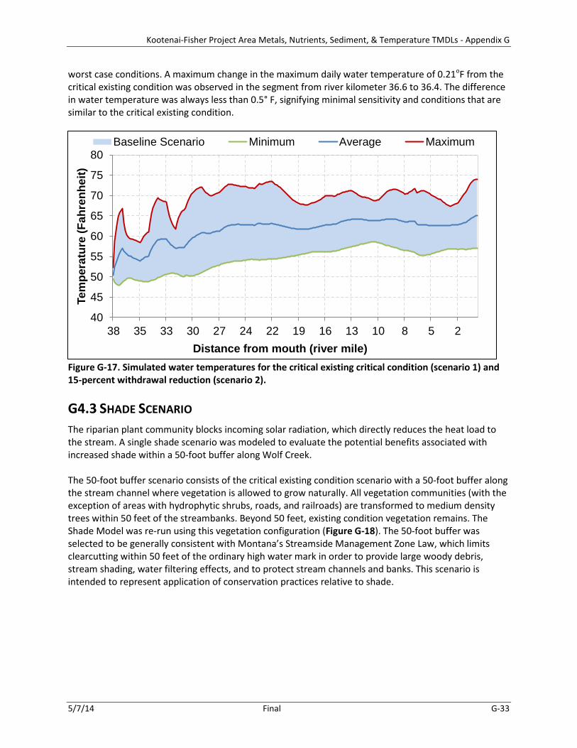
G4.2 WATER USE SCENARIO Irrigation (or other water withdrawals) depletes the volume of water in the stream and reduces instream volumetric heat capacity. Theoretically the reduced stream water volume heats up more quickly, and to a higher temperature, given the same amount of thermal input. A single water use scenario was modeled to evaluate the potential benefits associated with application of water use best management practices (scenario 2). In this scenario, the single irrigation withdrawal (see Attachment G-1 for information regarding the withdrawal) in the QUAL2K model is reduced by 15 percent. The Natural Resources Conservation Service Irrigation Guide (Natural Resources Conservation Service, 1997) states that improving an existing irrigation system often increases water application efficiency by more than 30 percent and installing a new system typically adds an additional 5 percent to 10 percent savings. These improvements in efficiency could be used to grow different crops, expand production, or withdraw less water from the stream. Since leaving additional water instream could lower the maximum daily temperature, converting efficiency savings to a lower amount of water usage is the focus of this scenario. However, per Montana’s water quality law, TMDL development cannot be construed to divest, impair, or diminish any water right recognized pursuant to Title 85 (Montana Code Annotated Section 75-5-705), so any voluntary water savings and subsequent instream flow augmentation must be done in a way that protects water rights. In the water use scenario, a 15 percent reduction in withdrawal volume was used to simulate the outcome of leaving some of the water saved by implementing improvements to the irrigation network instream. Fifteen percent was chosen to be a reasonable starting point, but as no detailed analysis was conducted of the irrigation network in the Wolf Creek watershed, this scenario is not a formal efficiency improvement goal; it is an example intended to represent application of water conservation practices for water withdrawals. The water temperatures for Wolf Creek in this scenario exhibited a very small incremental change (Figure G-17). The maximum change in the maximum daily water temperature is representative of the
40
45
50
55
60
65
70
75
80
38 35 33 30 27 24 22 19 16 13 10 8 5 2
Tem
pera
ture
(Fah
renh
eit)
Distance from mouth (river mile)
Baseline Scenario Minimum Average Maximum
Kootenai-Fisher Project Area Metals, Nutrients, Sediment, & Temperature TMDLs - Appendix G
5/7/14 Final G-33
worst case conditions. A maximum change in the maximum daily water temperature of 0.21oF from the critical existing condition was observed in the segment from river kilometer 36.6 to 36.4. The difference in water temperature was always less than 0.5° F, signifying minimal sensitivity and conditions that are similar to the critical existing condition.
Figure G-17. Simulated water temperatures for the critical existing critical condition (scenario 1) and 15-percent withdrawal reduction (scenario 2).
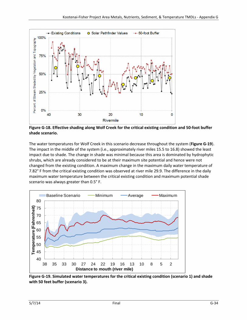
G4.3 SHADE SCENARIO The riparian plant community blocks incoming solar radiation, which directly reduces the heat load to the stream. A single shade scenario was modeled to evaluate the potential benefits associated with increased shade within a 50-foot buffer along Wolf Creek. The 50-foot buffer scenario consists of the critical existing condition scenario with a 50-foot buffer along the stream channel where vegetation is allowed to grow naturally. All vegetation communities (with the exception of areas with hydrophytic shrubs, roads, and railroads) are transformed to medium density trees within 50 feet of the streambanks. Beyond 50 feet, existing condition vegetation remains. The Shade Model was re-run using this vegetation configuration (Figure G-18). The 50-foot buffer was selected to be generally consistent with Montana’s Streamside Management Zone Law, which limits clearcutting within 50 feet of the ordinary high water mark in order to provide large woody debris, stream shading, water filtering effects, and to protect stream channels and banks. This scenario is intended to represent application of conservation practices relative to shade.
40
45
50
55
60
65
70
75
80
38 35 33 30 27 24 22 19 16 13 10 8 5 2
Tem
pera
ture
(Fah
renh
eit)
Distance from mouth (river mile)
Baseline Scenario Minimum Average Maximum
Kootenai-Fisher Project Area Metals, Nutrients, Sediment, & Temperature TMDLs - Appendix G
5/7/14 Final G-34
Figure G-18. Effective shading along Wolf Creek for the critical existing condition and 50-foot buffer shade scenario. The water temperatures for Wolf Creek in this scenario decrease throughout the system (Figure G-19). The impact in the middle of the system (i.e., approximately river miles 15.5 to 16.8) showed the least impact due to shade. The change in shade was minimal because this area is dominated by hydrophytic shrubs, which are already considered to be at their maximum site potential and hence were not changed from the existing condition. A maximum change in the maximum daily water temperature of 7.82° F from the critical existing condition was observed at river mile 29.9. The difference in the daily maximum water temperature between the critical existing condition and maximum potential shade scenario was always greater than 0.5° F.
Figure G-19. Simulated water temperatures for the critical existing condition (scenario 1) and shade with 50 feet buffer (scenario 3).
40
45
50
55
60
65
70
75
80
38 35 33 30 27 24 22 19 16 13 10 8 5 2
Tem
pera
ture
(Fah
renh
eit)
Distance to mouth (river mile)
Baseline Scenario Minimum Average Maximum
Kootenai-Fisher Project Area Metals, Nutrients, Sediment, & Temperature TMDLs - Appendix G
5/7/14 Final G-35
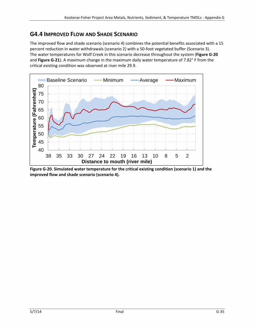
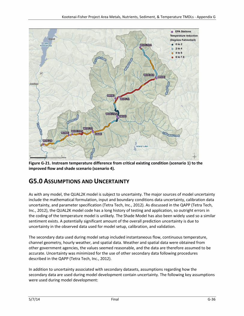
G4.4 IMPROVED FLOW AND SHADE SCENARIO The improved flow and shade scenario (scenario 4) combines the potential benefits associated with a 15 percent reduction in water withdrawals (scenario 2) with a 50-foot vegetated buffer (Scenario 3). The water temperatures for Wolf Creek in this scenario decrease throughout the system (Figure G-20 and Figure G-21). A maximum change in the maximum daily water temperature of 7.82° F from the critical existing condition was observed at river mile 29.9.
Figure G-20. Simulated water temperature for the critical existing condition (scenario 1) and the improved flow and shade scenario (scenario 4).
404550556065707580
38 35 33 30 27 24 22 19 16 13 10 8 5 2
Tem
pera
ture
(Fah
renh
eit)
Distance to mouth (river mile)
Baseline Scenario Minimum Average Maximum
Kootenai-Fisher Project Area Metals, Nutrients, Sediment, & Temperature TMDLs - Appendix G
5/7/14 Final G-36
Figure G-21. Instream temperature difference from critical existing condition (scenario 1) to the improved flow and shade scenario (scenario 4).
G5.0 ASSUMPTIONS AND UNCERTAINTY
As with any model, the QUAL2K model is subject to uncertainty. The major sources of model uncertainty include the mathematical formulation, input and boundary conditions data uncertainty, calibration data uncertainty, and parameter specification (Tetra Tech, Inc., 2012). As discussed in the QAPP (Tetra Tech, Inc., 2012), the QUAL2K model code has a long history of testing and application, so outright errors in the coding of the temperature model is unlikely. The Shade Model has also been widely used so a similar sentiment exists. A potentially significant amount of the overall prediction uncertainty is due to uncertainty in the observed data used for model setup, calibration, and validation. The secondary data used during model setup included instantaneous flow, continuous temperature, channel geometry, hourly weather, and spatial data. Weather and spatial data were obtained from other government agencies, the values seemed reasonable, and the data are therefore assumed to be accurate. Uncertainty was minimized for the use of other secondary data following procedures described in the QAPP (Tetra Tech, Inc., 2012). In addition to uncertainty associated with secondary datasets, assumptions regarding how the secondary data are used during model development contain uncertainty. The following key assumptions were used during model development:
Kootenai-Fisher Project Area Metals, Nutrients, Sediment, & Temperature TMDLs - Appendix G
5/7/14 Final G-37
• Wolf Creek can be divided into distinct segments, each considered homogeneous for shade, flow, and channel geometry characteristics. Monitoring sites at discrete locations were selected to be representative of segments of Wolf Creek.
• Stream meander and hyporheic flow paths (both of which may affect depth-velocity and temperature) are inherently represented during the estimation of various parameters (e.g., stream slope, channel geometry, and Manning’s roughness coefficient) for each segment.
• Weather conditions at the Fisher River RAWS, which were elevation-corrected, are representative of local weather conditions along Wolf Creek.
• Shade Model results are representative of riparian shading along segments of Wolf Creek. Shade Model development relied upon the following three estimations of riparian vegetation characteristics:
o Riparian vegetation communities were identified from visual interpretation of aerial imagery.
o Tree height and percent overhang were estimated from other similar studies conducted outside of the Wolf Creek watershed.
o Vegetation density was estimated using the NLCD and best professional judgment. Shade Model results were corroborated with field measured Solar PathfinderTM results and were found to be reasonable. The average absolute mean error is 7 percent. (i.e., the average error from the Shade Model output and Solar PathfinderTM measurements was 7 percent daily average shade).
• All of the cropland associated with water rights is fully irrigated. No field measurements of irrigation withdrawals or returns were available.
• Simulated diffuse flow rates are representative of groundwater inflow/outflow, irrigation diversion, irrigation return flow, and other sources of inflow and outflow not explicitly modeled. Diffuse flow rates were estimated using flow mass balance equations for each model reach.
• Shallow groundwater temperature is approximately 57.2° F (as the model was calibrated and validated), which were derived, in part, from the average of mean daily air temperatures from the preceding three months (May, June, and July).
Sensitivity analysis is the most widely applied approach for evaluating parameter uncertainty for complex simulation models. Although sensitivity analysis is limited in its ability to evaluate nonlinear interactions among multiple parameters, model sensitivity was evaluated by making changes to shade and water use (i.e., the key thermal mechanisms (Tetra Tech, Inc., 2012)) in separate model runs and evaluating the model response. The increased shade scenario (scenario 3) assumes that the system potential vegetation for the riparian area within 50 feet of the streambank is medium density trees (i.e., with the exception of areas currently dominated by hydrophytic shrubs or areas such as roads or railroads that no longer have the potential to support vegetation). The increased shade scenario (scenario 3) represents the maximum temperature benefit
Model Sensitivity to Water Withdrawals and Shade Model sensitivity to water withdrawal and shade was further evaluated by varying the amounts of water withdrawn and shade and re-running the model. To assess model sensitivity to water withdrawals, the point source abstractions representing the withdrawals (see Attachment G-1 for the withdrawals) were removed and the existing condition model was run to represent the maximum achievable change in water temperatures from changes in water use. To assess model sensitivity to shade, all vegetation was converted to high density trees (with the exception of roads, railroads, and hydrophytic shrubs) to represent the maximum potential shade. While not likely feasible, these conditions were run to assess model sensitivity. The results suggest that the model is not very sensitive to changes in water use but is sensitive to changes in shade.

Kootenai-Fisher Project Area Metals, Nutrients, Sediment, & Temperature TMDLs - Appendix G
5/7/14 Final G-38
that could be achieved over a time period long enough to allow vegetation to mature (tens of years). Therefore, temperature improvements in the short term are likely to be less than those identified in the scenario 3 results. Natural events such as flood and fire may also alter the maximum potential for the riparian vegetation or shift the time needed to achieve the maximum potential. This condition may not be achievable for all areas due to the coarse scale used to identify the current and potential shade conditions.
G6.0 MODEL USE AND LIMITATIONS
The model is only valid for summertime, low flow conditions and should not be used to evaluate high flow or other conditions. As described above, steps were taken to minimize uncertainty as much as possible. Despite the uncertainty, the model adequately addresses the primary questions:
1. What is the sensitivity of instream temperature to the following thermal mechanisms and stressors: shade, irrigation withdrawal and return?
2. What levels of reductions in controllable stressors are needed to achieve temperature standards?
The first principal study question can be answered using the calibrated and validated QUAL2K model for Wolf Creek. As previously discussed, Wolf Creek is sensitive to shade. The second principal study questions can be answered using the calibrated QUAL2K model and the scenarios developed to assess shade. Increasing riparian shading will decrease instream temperatures; however, there is uncertainty in the magnitude of temperature reduction necessary to achieve the temperature standard caused by uncertainty in the Shade Model results and QUAL2K model results. While a “good” model calibration was achieved, the overall Absolute Mean Error (AME) for the maximum daily temperature was 1.7° F. Montana’s temperature standard as applied to Wolf Creek is limited to an increase of 1° F. The model results, therefore, should be used with caution relative to the second primary question. However, in spite of the uncertainty, the magnitude of difference between the maximum daily temperatures under scenarios 1 and 4 is greater than the AME for most of the length of Wolf Creek (Figure G-22). This suggests that, on average5, a reduction of 4.6°F (range: 0.7° F to 7.8° F) is necessary to achieve the temperature standard in Wolf Creek.
5 Spatial average of the QUAL2K output at each element along the entire length of Wolf Creek.
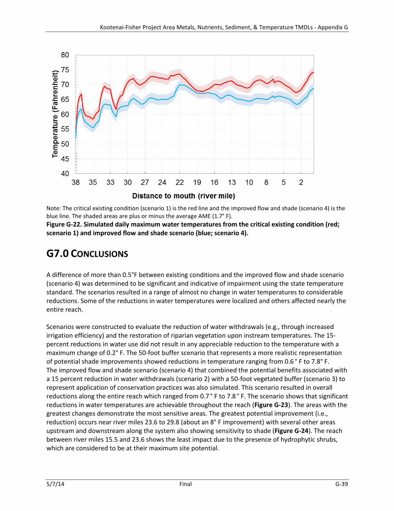
Kootenai-Fisher Project Area Metals, Nutrients, Sediment, & Temperature TMDLs - Appendix G
5/7/14 Final G-39
Note: The critical existing condition (scenario 1) is the red line and the improved flow and shade (scenario 4) is the blue line. The shaded areas are plus or minus the average AME (1.7° F). Figure G-22. Simulated daily maximum water temperatures from the critical existing condition (red; scenario 1) and improved flow and shade scenario (blue; scenario 4).
G7.0 CONCLUSIONS
A difference of more than 0.5°F between existing conditions and the improved flow and shade scenario (scenario 4) was determined to be significant and indicative of impairment using the state temperature standard. The scenarios resulted in a range of almost no change in water temperatures to considerable reductions. Some of the reductions in water temperatures were localized and others affected nearly the entire reach. Scenarios were constructed to evaluate the reduction of water withdrawals (e.g., through increased irrigation efficiency) and the restoration of riparian vegetation upon instream temperatures. The 15-percent reductions in water use did not result in any appreciable reduction to the temperature with a maximum change of 0.2° F. The 50-foot buffer scenario that represents a more realistic representation of potential shade improvements showed reductions in temperature ranging from 0.6 ° F to 7.8° F. The improved flow and shade scenario (scenario 4) that combined the potential benefits associated with a 15 percent reduction in water withdrawals (scenario 2) with a 50-foot vegetated buffer (scenario 3) to represent application of conservation practices was also simulated. This scenario resulted in overall reductions along the entire reach which ranged from 0.7 ° F to 7.8 ° F. The scenario shows that significant reductions in water temperatures are achievable throughout the reach (Figure G-23). The areas with the greatest changes demonstrate the most sensitive areas. The greatest potential improvement (i.e., reduction) occurs near river miles 23.6 to 29.8 (about an 8° F improvement) with several other areas upstream and downstream along the system also showing sensitivity to shade (Figure G-24). The reach between river miles 15.5 and 23.6 shows the least impact due to the presence of hydrophytic shrubs, which are considered to be at their maximum site potential.
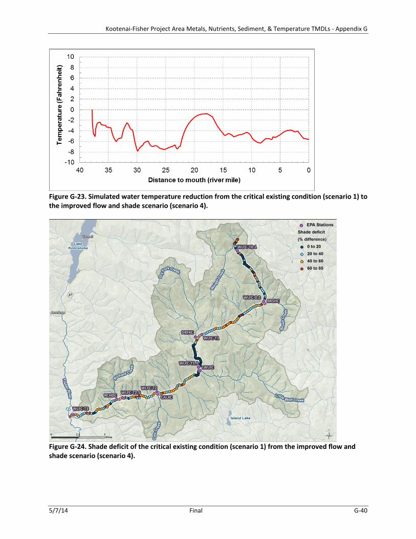
Kootenai-Fisher Project Area Metals, Nutrients, Sediment, & Temperature TMDLs - Appendix G
5/7/14 Final G-40
Figure G-23. Simulated water temperature reduction from the critical existing condition (scenario 1) to the improved flow and shade scenario (scenario 4).
Figure G-24. Shade deficit of the critical existing condition (scenario 1) from the improved flow and shade scenario (scenario 4).
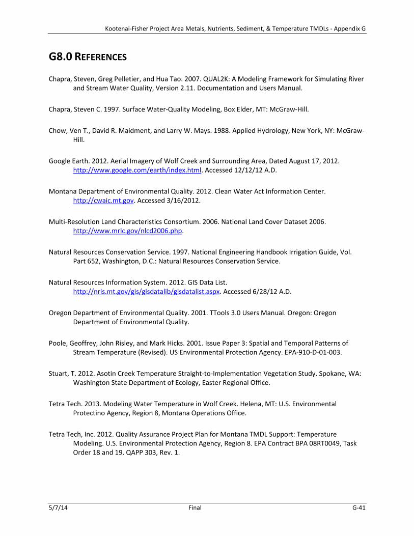
Kootenai-Fisher Project Area Metals, Nutrients, Sediment, & Temperature TMDLs - Appendix G
5/7/14 Final G-41
G8.0 REFERENCES
Chapra, Steven, Greg Pelletier, and Hua Tao. 2007. QUAL2K: A Modeling Framework for Simulating River and Stream Water Quality, Version 2.11. Documentation and Users Manual.
Chapra, Steven C. 1997. Surface Water-Quality Modeling, Box Elder, MT: McGraw-Hill.
Chow, Ven T., David R. Maidment, and Larry W. Mays. 1988. Applied Hydrology, New York, NY: McGraw-Hill.
Google Earth. 2012. Aerial Imagery of Wolf Creek and Surrounding Area, Dated August 17, 2012. http://www.google.com/earth/index.html. Accessed 12/12/12 A.D.
Montana Department of Environmental Quality. 2012. Clean Water Act Information Center. http://cwaic.mt.gov. Accessed 3/16/2012.
Multi-Resolution Land Characteristics Consortium. 2006. National Land Cover Dataset 2006. http://www.mrlc.gov/nlcd2006.php.
Natural Resources Conservation Service. 1997. National Engineering Handbook Irrigation Guide, Vol. Part 652, Washington, D.C.: Natural Resources Conservation Service.
Natural Resources Information System. 2012. GIS Data List. http://nris.mt.gov/gis/gisdatalib/gisdatalist.aspx. Accessed 6/28/12 A.D.
Oregon Department of Environmental Quality. 2001. TTools 3.0 Users Manual. Oregon: Oregon Department of Environmental Quality.
Poole, Geoffrey, John Risley, and Mark Hicks. 2001. Issue Paper 3: Spatial and Temporal Patterns of Stream Temperature (Revised). US Environmental Protection Agency. EPA-910-D-01-003.
Stuart, T. 2012. Asotin Creek Temperature Straight-to-Implementation Vegetation Study. Spokane, WA: Washington State Department of Ecology, Easter Regional Office.
Tetra Tech. 2013. Modeling Water Temperature in Wolf Creek. Helena, MT: U.S. Environmental Protectino Agency, Region 8, Montana Operations Office.
Tetra Tech, Inc. 2012. Quality Assurance Project Plan for Montana TMDL Support: Temperature Modeling. U.S. Environmental Protection Agency, Region 8. EPA Contract BPA 08RT0049, Task Order 18 and 19. QAPP 303, Rev. 1.

Kootenai-Fisher Project Area Metals, Nutrients, Sediment, & Temperature TMDLs - Appendix G
5/7/14 Final G-42
ATTACHMENT G-1 - FACTORS POTENTIALLY INFLUENCING STREAM TEMPERATURE IN WOLF CREEK
G1-1.0 INTRODUCTION
Stream temperature regimes are influenced by processes that are external to the stream as well as processes that occur within the stream and its associated riparian zone (Poole et al., 2001). Examples of factors external to the stream that can affect instream water temperatures include: topographic shade, land use/land cover (e.g., vegetation and the shading it provides, impervious surfaces), solar angle, meteorological conditions (e.g., precipitation, air temperature, cloud cover, relative humidity), groundwater exchange and temperature, and tributary inflow temperatures and volumes. The shape of the channel can also affect the temperature—wide shallow channels are more easily heated and cooled than deep, narrow channels. The amount of water in the stream is another factor influencing stream temperature regimes. Streams that carry large amounts of water resist heating and cooling, whereas temperature in small streams (or reduced flows) can be changed more easily. The following factors that may have an influence on stream temperatures in Wolf Creek are discussed below:
• Local/regional climate • Land ownership • Land use • Riparian vegetation • Shade • Hydrology • Point sources
G1-2.0 CLIMATE
The nearest weather station to the Wolf Creek watershed is the Hand Creek SNOpack TELemetry (SNOTEL) station (USS0014A14S, HANM8) (Figure G1-1). Average annual precipitation is 30.8 inches with the greatest amounts falling in June and November (Figure G1-2). Average maximum temperatures occur in July and August and are 74.8 °F and 74.7°F, respectively. It should be noted that the Hand Creek weather station is located at an elevation of 5,032 feet above mean sea level (MSL), compared to the impaired reach of Wolf Creek that ranges in elevation from approximately 2,500 to 3,740 feet above MSL. A Remote Automatic Weather Station (RAWS) named Fisher River (National Weather Service station ID 240118, RAWS ID: TS259) at 2,600 feet above MSL is 8 miles north of the mouth of Wolf Creek (Figure G1-2). This station records weather data hourly whereas stations US0014A14S record weather data daily. Thus, Fisher River RAWS hourly temperature data will be used to develop the QUAL2K inputs.
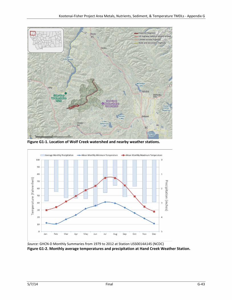
Kootenai-Fisher Project Area Metals, Nutrients, Sediment, & Temperature TMDLs - Appendix G
5/7/14 Final G-43
Figure G1-1. Location of Wolf Creek watershed and nearby weather stations.
Source: GHCN-D Monthly Summaries from 1979 to 2012 at Station USS0014A14S (NCDC) Figure G1-2. Monthly average temperatures and precipitation at Hand Creek Weather Station.
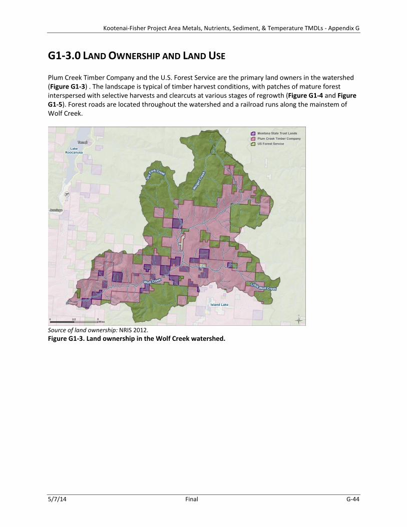
Kootenai-Fisher Project Area Metals, Nutrients, Sediment, & Temperature TMDLs - Appendix G
5/7/14 Final G-44
G1-3.0 LAND OWNERSHIP AND LAND USE
Plum Creek Timber Company and the U.S. Forest Service are the primary land owners in the watershed (Figure G1-3) . The landscape is typical of timber harvest conditions, with patches of mature forest interspersed with selective harvests and clearcuts at various stages of regrowth (Figure G1-4 and Figure G1-5). Forest roads are located throughout the watershed and a railroad runs along the mainstem of Wolf Creek.
Source of land ownership: NRIS 2012. Figure G1-3. Land ownership in the Wolf Creek watershed.
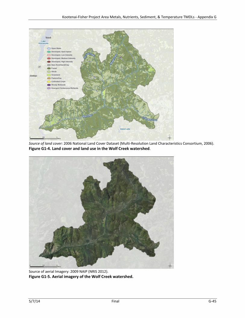
Kootenai-Fisher Project Area Metals, Nutrients, Sediment, & Temperature TMDLs - Appendix G
5/7/14 Final G-45
Source of land cover: 2006 National Land Cover Dataset (Multi-Resolution Land Characteristics Consortium, 2006). Figure G1-4. Land cover and land use in the Wolf Creek watershed.
Source of aerial Imagery: 2009 NAIP (NRIS 2012). Figure G1-5. Aerial imagery of the Wolf Creek watershed.

Kootenai-Fisher Project Area Metals, Nutrients, Sediment, & Temperature TMDLs - Appendix G
5/7/14 Final G-46
G1-4.0 EXISTING RIPARIAN VEGETATION
Vegetation communities between the shade monitoring sites were visually characterized based on aerial imagery (Google Earth, 2012) with qualitative field verification conducted during a September 11, 2012 shade monitoring event. Observed vegetative communities within 150 feet of the stream centerline were classified as trees, shrubs, herbaceous. Areas without vegetation, such as bare earth or roads, were also identified. Trees were further divided into the following classes based on percent canopy cover derived from the 2001 NLCD (Figure G1-6):
• High density (75 to 100 percent cover) • Medium density (51 to 74 percent cover) • Low density (25 to 50 percent cover) • Sparse density (less than 24 percent cover)
Herbaceous and shrubs are the most common cover types along Wolf Creek, followed by medium and high density trees (Table G1-1). Sparse trees, roads, and bare ground comprise only a small percentage of the riparian area.
Figure G1-6. Vegetation mapping example for Wolf Creek.
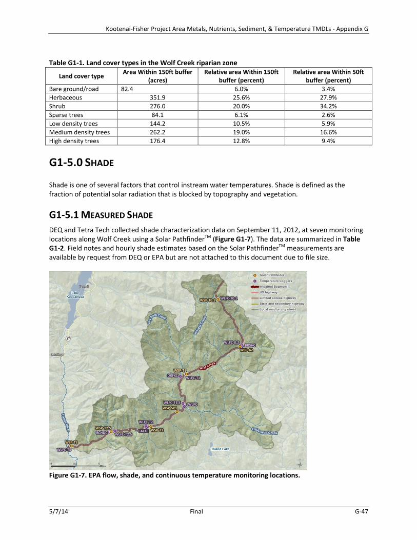
Kootenai-Fisher Project Area Metals, Nutrients, Sediment, & Temperature TMDLs - Appendix G
5/7/14 Final G-47
Table G1-1. Land cover types in the Wolf Creek riparian zone
Land cover type Area Within 150ft buffer (acres)
Relative area Within 150ft buffer (percent)
Relative area Within 50ft buffer (percent)
Bare ground/road 82.4 6.0% 3.4% Herbaceous 351.9 25.6% 27.9% Shrub 276.0 20.0% 34.2% Sparse trees 84.1 6.1% 2.6% Low density trees 144.2 10.5% 5.9% Medium density trees 262.2 19.0% 16.6% High density trees 176.4 12.8% 9.4%
G1-5.0 SHADE
Shade is one of several factors that control instream water temperatures. Shade is defined as the fraction of potential solar radiation that is blocked by topography and vegetation.
G1-5.1 MEASURED SHADE DEQ and Tetra Tech collected shade characterization data on September 11, 2012, at seven monitoring locations along Wolf Creek using a Solar PathfinderTM (Figure G1-7). The data are summarized in Table G1-2. Field notes and hourly shade estimates based on the Solar PathfinderTM measurements are available by request from DEQ or EPA but are not attached to this document due to file size.
Figure G1-7. EPA flow, shade, and continuous temperature monitoring locations.
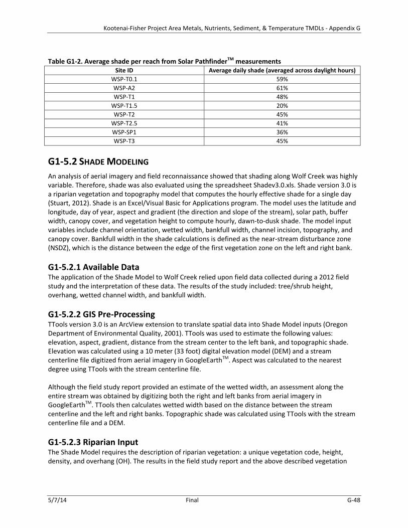
Kootenai-Fisher Project Area Metals, Nutrients, Sediment, & Temperature TMDLs - Appendix G
5/7/14 Final G-48
Table G1-2. Average shade per reach from Solar PathfinderTM measurements
Site ID Average daily shade (averaged across daylight hours) WSP-T0.1 59% WSP-A2 61% WSP-T1 48%
WSP-T1.5 20% WSP-T2 45%
WSP-T2.5 41% WSP-SP1 36% WSP-T3 45%
G1-5.2 SHADE MODELING An analysis of aerial imagery and field reconnaissance showed that shading along Wolf Creek was highly variable. Therefore, shade was also evaluated using the spreadsheet Shadev3.0.xls. Shade version 3.0 is a riparian vegetation and topography model that computes the hourly effective shade for a single day (Stuart, 2012). Shade is an Excel/Visual Basic for Applications program. The model uses the latitude and longitude, day of year, aspect and gradient (the direction and slope of the stream), solar path, buffer width, canopy cover, and vegetation height to compute hourly, dawn-to-dusk shade. The model input variables include channel orientation, wetted width, bankfull width, channel incision, topography, and canopy cover. Bankfull width in the shade calculations is defined as the near-stream disturbance zone (NSDZ), which is the distance between the edge of the first vegetation zone on the left and right bank. G1-5.2.1 Available Data The application of the Shade Model to Wolf Creek relied upon field data collected during a 2012 field study and the interpretation of these data. The results of the study included: tree/shrub height, overhang, wetted channel width, and bankfull width. G1-5.2.2 GIS Pre-Processing TTools version 3.0 is an ArcView extension to translate spatial data into Shade Model inputs (Oregon Department of Environmental Quality, 2001). TTools was used to estimate the following values: elevation, aspect, gradient, distance from the stream center to the left bank, and topographic shade. Elevation was calculated using a 10 meter (33 foot) digital elevation model (DEM) and a stream centerline file digitized from aerial imagery in GoogleEarthTM. Aspect was calculated to the nearest degree using TTools with the stream centerline file. Although the field study report provided an estimate of the wetted width, an assessment along the entire stream was obtained by digitizing both the right and left banks from aerial imagery in GoogleEarthTM. TTools then calculates wetted width based on the distance between the stream centerline and the left and right banks. Topographic shade was calculated using TTools with the stream centerline file and a DEM. G1-5.2.3 Riparian Input The Shade Model requires the description of riparian vegetation: a unique vegetation code, height, density, and overhang (OH). The results in the field study report and the above described vegetation
Kootenai-Fisher Project Area Metals, Nutrients, Sediment, & Temperature TMDLs - Appendix G
5/7/14 Final G-49
mapping were used to develop a riparian description table (Table G1-3). Vegetation descriptions used the average value for tree/shrub height and overhang from field observation. Table G1-3. Vegetation input values for the Shade Model
Attribute Value Basis Trees
Height 20.9 meters (69 feet) Average of field values across all Solar PathfinderTM sites. Density Variable 2006 NLCD. Overhang 2.1 meters (6.9 feet) Estimated as 10% of height (Stuart 2012).
Shrubs Height 4.9 meters (16 feet) Average of field values across all Solar PathfinderTM sites. Density 90% Ocular estimate based on aerial imagery. Overhang 1.2 meter (3.9 feet) Estimated as 25% of height (Shumar and de Varona 2009)
Herbaceous Height 1 meter (3.3 feet) Estimated average based on site reconnaissance (September 2012). Density 100% Estimated average based on site reconnaissance (September 2012). Overhang 0 meters Estimated based on site reconnaissance (September 2012). G1-5.2.4 Shade Input The Shade Model inputs are riparian zones, reach length, channel incision, elevation, aspect, wetted width, near-stream disturbance zone width, distance from the bank to the center of the stream, and topographic shade. Input for the riparian zone is presented above in Table G1-3. The Shade Model requires reach lengths be an equal interval. The reaches in the field study report were not at an equal interval and were very widely spaced. A uniform reach length interval of 30 meters (98 feet) was used. Channel incision was estimated from an examination of field photos. Incision is the vertical drop from the bankfull edge to the water surface, and was estimated at 0.3 meter (1 foot). The remaining variables were computed as part of the GIS pre-processing described above.
G1-5.3 SHADE MODEL RESULTS The current longitudinal effective shade profile generated from the Shade Model and the Solar PathfinderTM measurements are presented in Figure G1-8.
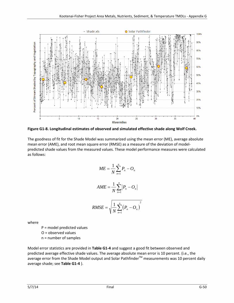
Kootenai-Fisher Project Area Metals, Nutrients, Sediment, & Temperature TMDLs - Appendix G
5/7/14 Final G-50
Figure G1-8. Longitudinal estimates of observed and simulated effective shade along Wolf Creek. The goodness of fit for the Shade Model was summarized using the mean error (ME), average absolute mean error (AME), and root mean square error (RMSE) as a measure of the deviation of model-predicted shade values from the measured values. These model performance measures were calculated as follows:
n
n
nn OP
NME −= ∑
=1
1
∑=
−=n
nnn OP
NAME
1
1
( )2
1
1 ∑=
−=n
nnn OP
NRMSE
where P = model predicted values O = observed values n = number of samples Model error statistics are provided in Table G1-4 and suggest a good fit between observed and predicted average effective shade values. The average absolute mean error is 10 percent. (i.e., the average error from the Shade Model output and Solar PathfinderTM measurements was 10 percent daily average shade; see Table G1-4 ).
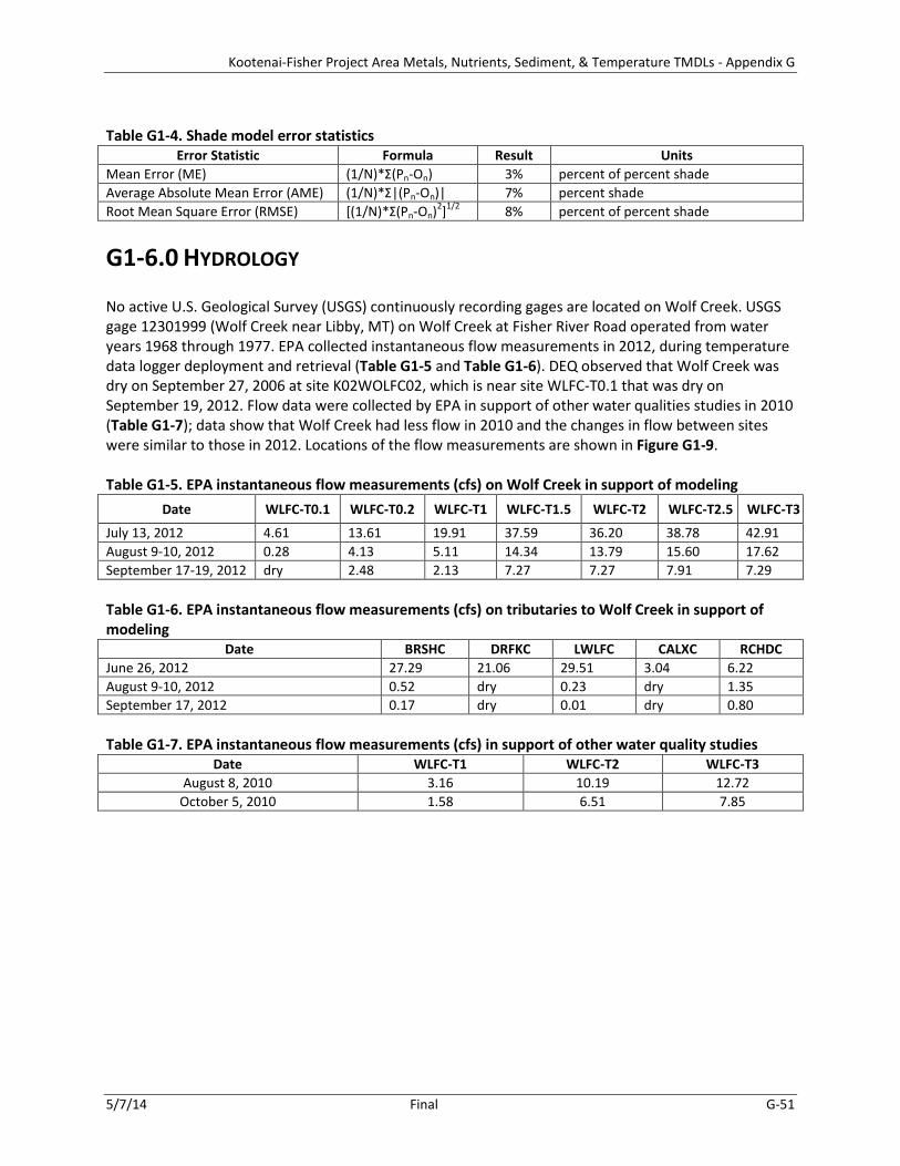
Kootenai-Fisher Project Area Metals, Nutrients, Sediment, & Temperature TMDLs - Appendix G
5/7/14 Final G-51
Table G1-4. Shade model error statistics
Error Statistic Formula Result Units Mean Error (ME) (1/N)*Σ(Pn-On) 3% percent of percent shade Average Absolute Mean Error (AME) (1/N)*Σ|(Pn-On)| 7% percent shade Root Mean Square Error (RMSE) [(1/N)*Σ(Pn-On)2]1/2 8% percent of percent shade
G1-6.0 HYDROLOGY
No active U.S. Geological Survey (USGS) continuously recording gages are located on Wolf Creek. USGS gage 12301999 (Wolf Creek near Libby, MT) on Wolf Creek at Fisher River Road operated from water years 1968 through 1977. EPA collected instantaneous flow measurements in 2012, during temperature data logger deployment and retrieval (Table G1-5 and Table G1-6). DEQ observed that Wolf Creek was dry on September 27, 2006 at site K02WOLFC02, which is near site WLFC-T0.1 that was dry on September 19, 2012. Flow data were collected by EPA in support of other water qualities studies in 2010 (Table G1-7); data show that Wolf Creek had less flow in 2010 and the changes in flow between sites were similar to those in 2012. Locations of the flow measurements are shown in Figure G1-9. Table G1-5. EPA instantaneous flow measurements (cfs) on Wolf Creek in support of modeling
Date WLFC-T0.1 WLFC-T0.2 WLFC-T1 WLFC-T1.5 WLFC-T2 WLFC-T2.5 WLFC-T3
July 13, 2012 4.61 13.61 19.91 37.59 36.20 38.78 42.91 August 9-10, 2012 0.28 4.13 5.11 14.34 13.79 15.60 17.62 September 17-19, 2012 dry 2.48 2.13 7.27 7.27 7.91 7.29 Table G1-6. EPA instantaneous flow measurements (cfs) on tributaries to Wolf Creek in support of modeling
Date BRSHC DRFKC LWLFC CALXC RCHDC June 26, 2012 27.29 21.06 29.51 3.04 6.22 August 9-10, 2012 0.52 dry 0.23 dry 1.35 September 17, 2012 0.17 dry 0.01 dry 0.80 Table G1-7. EPA instantaneous flow measurements (cfs) in support of other water quality studies
Date WLFC-T1 WLFC-T2 WLFC-T3 August 8, 2010 3.16 10.19 12.72
October 5, 2010 1.58 6.51 7.85
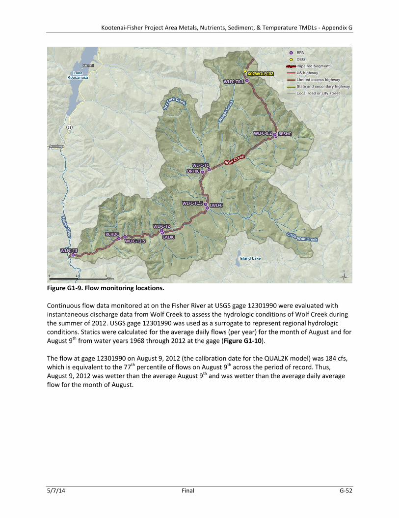
Kootenai-Fisher Project Area Metals, Nutrients, Sediment, & Temperature TMDLs - Appendix G
5/7/14 Final G-52
Figure G1-9. Flow monitoring locations. Continuous flow data monitored at on the Fisher River at USGS gage 12301990 were evaluated with instantaneous discharge data from Wolf Creek to assess the hydrologic conditions of Wolf Creek during the summer of 2012. USGS gage 12301990 was used as a surrogate to represent regional hydrologic conditions. Statics were calculated for the average daily flows (per year) for the month of August and for August 9th from water years 1968 through 2012 at the gage (Figure G1-10). The flow at gage 12301990 on August 9, 2012 (the calibration date for the QUAL2K model) was 184 cfs, which is equivalent to the 77th percentile of flows on August 9th across the period of record. Thus, August 9, 2012 was wetter than the average August 9th and was wetter than the average daily average flow for the month of August.

Kootenai-Fisher Project Area Metals, Nutrients, Sediment, & Temperature TMDLs - Appendix G
5/7/14 Final G-53
Note: “August” represents the daily average flow for the month of August per year (i.e., the average of 31 daily average flows) Figure G1-10. Flow analysis with USGS gage 12302055 (Fisher River near Libby, MT).
G1-7.0 FLOW MODIFICATION
Based on review of aerial photographs and online water rights data (ftp://nris.mt.gov/dnrc), there are surface and groundwater diversions in the Wolf Creek watershed that support a variety of uses (Figure G1-11). “Points of diversion” and “places of use” spatial data were obtained from the Montana Natural Resource Information System (Natural Resources Information System, 2012). Of the 17 diversions in the Wolf Creek watershed, 3 were directly from Wolf Creek. The permit for the mining water diversion has been terminated. Of the remaining permits, one is used for livestock and the other is used for flood irrigation (Figure G1-11 and Table G1-8). It is estimated that up to 1.78 cfs may be withdrawn from Wolf Creek on a daily basis during July and August (Table G1-8).
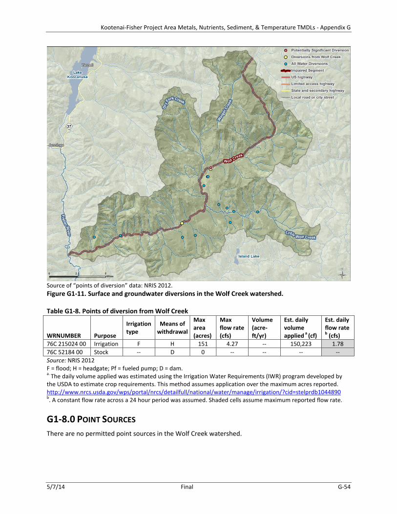
Kootenai-Fisher Project Area Metals, Nutrients, Sediment, & Temperature TMDLs - Appendix G
5/7/14 Final G-54
Source of “points of diversion” data: NRIS 2012. Figure G1-11. Surface and groundwater diversions in the Wolf Creek watershed. Table G1-8. Points of diversion from Wolf Creek
WRNUMBER Purpose
Irrigation type
Means of withdrawal
Max area (acres)
Max flow rate (cfs)
Volume (acre-ft/yr)
Est. daily volume applied a (cf)
Est. daily flow rate
b (cfs) 76C 215024 00 Irrigation F H 151 4.27 -- 150,223 1.78 76C 52184 00 Stock -- D 0 -- -- -- -- Source: NRIS 2012 F = flood; H = headgate; Pf = fueled pump; D = dam. a. The daily volume applied was estimated using the Irrigation Water Requirements (IWR) program developed by the USDA to estimate crop requirements. This method assumes application over the maximum acres reported. http://www.nrcs.usda.gov/wps/portal/nrcs/detailfull/national/water/manage/irrigation/?cid=stelprdb1044890 b. A constant flow rate across a 24 hour period was assumed. Shaded cells assume maximum reported flow rate.
G1-8.0 POINT SOURCES There are no permitted point sources in the Wolf Creek watershed.