appendix a hinode image gallery - link.springer.com978-981-10-7742-5/1.pdf · 266 a hinode image...

Appendix AHinode Image Gallery

A large number of images were acquired with the three telescopes onboardHinode in its first 10 years. Remarkable images, which are impressive to not onlyresearchers but also the general public, have been released via various forms ofmedia. This image gallery is a collection of some of the released images. Thecopyright of the images in the gallery is JAXA/NAOJ/Hinode,1 if not mentioned.

A.1 Quiet Sun

Fig. A.1 Solar granulation, visible everywhere on the solar surface. The photospheric (left, G-band) and chromospheric (right, Ca II H) images, captured by the Solar Optical Telescope (SOT)broadband filter imager with a spatial resolution of 0.2 arcsec (equivalent to 150 km on the solarsurface)

1Japan Aerospace Exploration Agency/National Astronomical Observatory of Japan/Hinode.

© Springer Nature Singapore Pte Ltd. 2018T. Shimizu et al. (eds.), First Ten Years of Hinode Solar On-Orbit Observatory,Astrophysics and Space Science Library 449,https://doi.org/10.1007/978-981-10-7742-5

263

https://doi.org/10.1007/978-981-10-7742-5

264 A Hinode Image Gallery

Fig. A.2 Magnetic flux patches distributed in the northern polar region. Owing to its high spatialresolution, the SOT observations provide accurate measurements of the spatial distribution ofmagnetic flux in the polar regions of the Sun in monthly intervals. These regions are difficultto view from the Earth due to foreshortening. The high spatial resolution observations allowed usto resolve magnetic flux patches with a magnetic flux density higher than 1000 Gauss (0.1 Tesla).This magnetic field map was measured on 20 September 2008 (top) and 9 October 2011 (bottom).The cross mark is the location of the North Pole, and each white line shows 85, 80, 75, 70, and 65ı

in heliographic latitude from the polar side. Red and blue colors represent positive and negativemagnetic polarity, respectively

A Hinode Image Gallery 265

Fig. A.3 A panorama map of magnetic flux at the northern polar region on September 2007. The360ı coverage in the heliographic longitude is achieved via magnetic field measurements carriedout every few days in a month. The cross mark is the location of the North Pole, and each whitecircle shows 85, 80, 75, and 70ı in heliographic latitude from the polar side. Red and blue colorsrepresent positive and negative magnetic polarity, respectively


A.2 Sunspots

Fig. A.4 “Japan” sunspot, which was the main sunspot in active region NOAA (National Oceanicand Atmospheric Administration) 10953 on 3 May 2007. The name comes from the fact that theoverall shape of the umbrae is similar to the islands of Japan. This image was taken with the bluecontinuum filter by the SOT


Fig. A.5 Active region NOAA 11429 on 8 March 2012, which produced X-class flares on 7 March2012. This image was taken with the blue continuum filter by the SOT

Fig. A.6 Active region NOAA 11429 on 6 March 2012, recorded a few hours before the startof an X-class flare. Vector magnetic field (left) map and sunspot continuum image (right), derivedfrom the spectropolarimeter data. The SOT’s spectropolarimeter records the full-polarization states(Stokes I, Q, U, and V) of line profiles of two magnetically sensitive Fe I lines at 630.15 and630.25 nm, allowing us to determine the magnetic flux vectors accurately with a spatial resolutionof 0.3 arcsec. Red and blue are the positive and negative polarities of magnetic flux, respectively,and arrows represent the direction of magnetic field at the solar surface


Fig. A.7 A large emerging flux region appeared from 30 to 31 December 2009 in active regionNOAA 11039. The SOT captured the totality of the evolution, from the birth of the pores to thedevelopment of the bipolar pair of sunspots with Ca II H filter


Fig. A.8 Active region NOAA 11339, rotated from behind the east limb in early November 2011.An X-class flare was produced about 10 h after these images were taken. Taken by the SOT withCa II H (top) and G-band filters (bottom)


Fig. A.9 A moderate-sized sunspot observed by the SOT. Filtergrams with chromospheric Ca IIH filter (top) and G-band filter (middle) and magnetogram (bottom)


Fig. A.10 Active region NOAA 12192 on 24 October 2014, recorded by the SOT: highest resolu-tion G-band image (top), continuum image (middle), and line-of-sight magnetogram (bottom). TheG-band’s field of view (108 � 84 arcsec, check) could capture only a limited area of this sunspotgroup. The size of the sunspot group is about 66 times larger than the size of the Earth, which hasbeen considered to be the largest since 18 November 1990. In the magnetogram, white and blackcorrespond to positive and negative magnetic polarity, respectively


A.3 Chromosphere

Fig. A.11 The solar limb, observed by the SOT with a Ca II H filter, showing dynamical behaviorsof chromospheric spicules. The chromosphere, the interface layer between the photosphere and thecorona, consists of large number of dynamic straw-like features known as spicules

Fig. A.12 High-resolution image of the solar limb showing fine structures of spicules, obtainedby the SOT with a Ca II H filter on 22 November 2006


Fig. A.13 Discovery of Alfvén waves. The time series of high-resolution Ca II H images taken bythe SOT has revealed transversal oscillations of minuscule magnetic structures, such as prominencethreads and spicules, with small amplitude. These oscillations are thought to be a signature ofmagnetohydrodynamic waves along the magnetic structures. Horizontally oriented threads at theupper portion of this photograph show oscillations in the up-and-down direction


Fig. A.14 A comparison of the chromospheric and photospheric images of the solar limb wherea large sunspot is located. The chromospheric image was taken with Ca II H filter, whereas thephotospheric image was taken with G-band filter. The region in and around the large sunspotshowed dynamical behaviors of the chromosphere including transient heating and plasma ejections


Fig. A.15 A giant chromospheric jet, captured by the SOT with Ca II H filter. Chromosphericmaterials were ejected obliquely upward with a transient heating of the chromospheric material atthe base. The ejections may reach beyond a few 10,000 km


Fig. A.16 A chromospheric jet observed by the SOT with Ca II H filter. The footpoint region ofthe jet is the brightest under the Ca II H filter, indicating that chromospheric plasma is transientlyheated


Fig. A.17 Dynamical fine structure in chromospheric prominence. The Ca II H images from theSOT are used to investigate dynamical behaviors of chromospheric materials in the prominence,including Kelvin-Helmholtz instability


Fig. A.18 Chromospheric materials erupting above the east limb, captured by the SOT with Ca IIH filter


A.4 Corona

Fig. A.19 Soft X-ray corona, captured by Hinode’s X-Ray Telescope (XRT). The XRT has aspatial resolution of about 1 arcsec, covering the entire solar disk when the spacecraft is pointingdirectly at the disk center


Fig. A.20 Soft X-ray corona on 9 December 2010. The coronal features look like the face of aman. The image was taken by the XRT


Fig. A.21 Soft X-ray corona in the solar minimum. The image was taken by the XRT on 11 March2008. A lot of small bright points, called X-ray bright points (XBPs), are distributed over the entiredisk in the solar minimum


Fig. A.22 The solar cycle seen in soft X-ray corona. The XRT has taken a unique set of XRTsynoptic data, which are the full-disk images only taken twice per day when the spacecraft isdirected to the disk center. The series of X-ray images at the upper portion show the yearlyevolution of the X-ray corona from 2008 to 2014. The image at the lower left is taken in 2008,when it is in the solar minimum, whereas that in the lower right is in 2014, when it is in the solarmaximum


Fig. A.23 Soft X-ray image of an active region, taken by the XRT. At the low-intensity regionlocated at the left side of the bright active region, it was found that the coronal plasma iscontinuously outflowing along the magnetic field lines upwardly at about 140 km s�1. This outflowis considered to be a source of slow solar winds

Fig. A.24 Soft X-ray image of a polar region, taken by the XRT. The coronal hole located atpolar regions is considered to be the source of fast solar winds with their speed being higher than700 km s�1. High cadence observations of XRT have revealed frequent occurrence of X-ray jets


Fig. A.25 The solar corona observed by the Extreme ultraviolet Imaging Spectrometer (EIS)on 4 December 2010. Many spectral emission lines in EUV wavelength originate in the coronaand transition region. The excitation of each spectral line depends on the temperature of plasma,determining the amount of plasma at the excitation temperature of each spectral line. From theupper left to the lower right, the temperature of the plasma is increased from the chromospherictemperature (He II) to the coronal temperatures (Fe XI to Fe XVI). Because of the narrow EIS fieldof view, the full images of the Sun were created from the data acquired at 13 different spacecraftpointing coordinates

Fig. A.26 The composite images of the solar corona on 1 February 2011 (left) and 4 December2010 (right). Images of Si VII, Fe XII, and Fe XV lines measured with EIS are used to createthese composite images. Blue indicates the lower temperature corona, whereas red shows a highertemperature, indicating that the solar corona consists of plasma at a range of temperatures


A.5 Flares and Eruptions

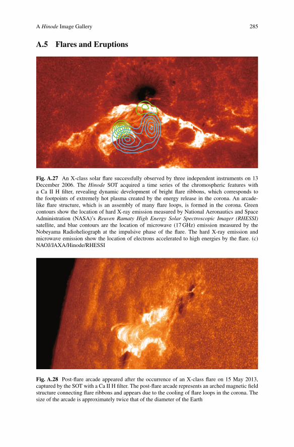
Fig. A.27 An X-class solar flare successfully observed by three independent instruments on 13December 2006. The Hinode SOT acquired a time series of the chromospheric features witha Ca II H filter, revealing dynamic development of bright flare ribbons, which corresponds tothe footpoints of extremely hot plasma created by the energy release in the corona. An arcade-like flare structure, which is an assembly of many flare loops, is formed in the corona. Greencontours show the location of hard X-ray emission measured by National Aeronautics and SpaceAdministration (NASA)’s Reuven Ramaty High Energy Solar Spectroscopic Imager (RHESSI)satellite, and blue contours are the location of microwave (17 GHz) emission measured by theNobeyama Radioheliograph at the impulsive phase of the flare. The hard X-ray emission andmicrowave emission show the location of electrons accelerated to high energies by the flare. (c)NAOJ/JAXA/Hinode/RHESSI

Fig. A.28 Post-flare arcade appeared after the occurrence of an X-class flare on 15 May 2013,captured by the SOT with a Ca II H filter. The post-flare arcade represents an arched magnetic fieldstructure connecting flare ribbons and appears due to the cooling of flare loops in the corona. Thesize of the arcade is approximately twice that of the diameter of the Earth


Fig. A.29 SOT observation of a white light flare on 14 December 2006. White light emissions mayappear along with the occurrence of solar flares. In this G-band image, bright emissions are seenin the lower left portion of the sunspot group. Comparing the intensity of the emission with that ofthe hard X-ray flux measured with RHESSI, highly accelerated electrons contribute significantly tothe appearance of white light emissions, which have been one of the mysteries since the discoveryof white light flares about 150 years ago


Fig. A.30 Time series of soft X-ray images by XRT on 9 April 2008, showing the temporalevolution of coronal magnetic structures when the coronal materials are suddenly ejected. Suchejections are called coronal mass ejections (CME), which are one of main sources of magneticstorms on Earth


Fig. A.31 The first large flare in the solar cycle 24 successfully captured by the SOT. A compositeimage of two Ca II H images with different exposure times. This X-class flare occurred on 15February 2011, which is more than 4 years after the previous X-class flare

Fig. A.32 A map of vector magnetic fields at the photosphere, derived from the SOT, for theX-class flare on 15 February 2011. White and black are positive and negative magnetic polarity,respectively. Blue arrows show the direction of horizontal magnetic fields


A.6 Astronomical Events

Fig. A.33 A total eclipse encountered in orbit on 19 March 2007. This eclipse was visible fromeastern Asia and parts of northern Alaska with the eclipse magnitude reaching 0.8754 on theground. Hinode was the only witness of the episode for the totality, which was visible from theorbit. This is the soft X-ray images from the XRT


Fig. A.34 A blue continuum image acquired by the SOT during an eclipse on 19 March 2007.The dark shadow is the partial limb of the moon, showing high mountains and valleys located atthe limb. The highest spatial resolution of the SOT is 0.2 arcsec, corresponding to 0.4 km on thesurface of the moon


Fig. A.35 An annular eclipse from space, only viewed from Hinode on 4 January 2011. This isthe soft X-ray image acquired by the XRT at the time of the annular eclipse. The dark shadow isthe silhouette of the moon


Fig. A.36 Transit of Mercury across the Sun on 9 November 2006, which occurred about onemonth after Hinode’s telescopes had begun observations. This image is G-band image recorded bythe SOT at the third contact (interior egress). The diameter of Mercury is approximately 10 arcsec


Fig. A.37 Mercury captured in soft X-ray images on 9 November 2006. The Mercury is observedas a small dark disk in front of soft X-rays from the coronal plasma. These images were taken bythe XRT when the Mercury was approaching the southeast portion of the solar limb


Fig. A.38 Comet Lovejoy, formally designated C/2011 W3 (Lovejoy), successfully captured bythe SOT. This comet was discovered by an amateur astronomer in November 2011. It passedthrough the Sun’s corona on 16 December 2011. The closest distance to the solar surface wasabout 140,000 km (0.2 solar radius). The SOT captured the comet core with a short tail in visiblelight, along with the very bright visible solar disk


Fig. A.39 On 20 May 2012, an annular eclipse was visible from a 240 to 300 km wide track thattraversed eastern Asia, the northern Pacific Ocean, and the western United States. From the orbit,Hinode observed this as a partial eclipse


Fig. A.40 Transit of Venus on 5 June 2012, observed by the XRT. The shadow disk is Venus


Fig. A.41 Transit of Venus on 5/6 June 2012, observed by the SOT with a Ca II H filter.The shadow disk is Venus and its diameter is 57.8 arcsec. The limb of Venus in front of thechromospheric atmosphere above the solar limb shows a bright arc, which is caused by scatteringof the solar radiation in the Venusian atmosphere


Fig. A.42 Another Ca II H image taken by the SOT during the transit of Venus on 5/6 June 2012.This image was taken shortly after the second contact (interior ingress)


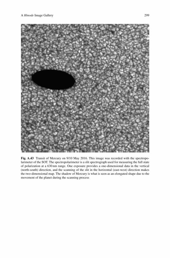
Fig. A.43 Transit of Mercury on 9/10 May 2016. This image was recorded with the spectropo-larimeter of the SOT. The spectropolarimeter is a slit spectrograph used for measuring the full stateof polarization at a 630 nm range. One exposure provides a one-dimensional data in the vertical(north-south) direction, and the scanning of the slit in the horizontal (east-west) direction makesthe two-dimensional map. The shadow of Mercury is what is seen as an elongated shape due to themovement of the planet during the scanning process

Index

Symbols11-year sunspot cycle, 223D magnetic structure, 115

Aabundance, 96, 99acceleration, 96ACE, 48acoustic heating theory, 24active region, 55, 126, 266, 283active region expansion, 25Alfvén wave, 32, 33, 56, 67, 80, 96, 156, 273Alfvén speed, 138ambipolar diffusion, 213annular eclipse, 291, 295astronomy educator, 256Astrophysics Data System (ADS), 11Atacama Large Millimeter/submillimeter

Array (ALMA),240, 247

axial dipole magnetic dipole moment, 175

Bbackside-illuminated CCD, 44boundary value problem, 117breakout model, 150bright point, 21Broad-band Filter Imager

(BFI), 28butterfly diagram, 174

Ccall for proposal, 248canopy structure, 23Chandra, 45Chief Observer (CO), 13Chief Planner (CP), 13chromosphere, 54, 188, 201, 211, 232chromospheric evaporation, 56, 88, 90, 135,

139, 225chromospheric jet, 35, 36, 203, 275, 276Chromospheric LAyer SpectroPolarimeter 2

(CLASP2), 237Chromospheric Lyman-Alpha Spectro-

Polarimeter (CLASP), 235collisional, 211collisionless plasma, 221comet Lovejoy, 294conductive cooling, 142continuous plasma flow, 47convection, 162convective collapse, 21, 28, 163convective motion, 23, 66Coriolis effect, 23corona, 27, 54, 211, 232, 279, 280, 284coronal dimming, 154coronal heating, 23, 31, 55, 65, 80, 203, 222,

238coronal hole, 67, 71, 96, 283coronal loop, 67, 79coronal magnetic field, 115coronal mass ejection, 27, 132, 141, 149, 287Coulomb collision, 221

© Springer Nature Singapore Pte Ltd. 2018T. Shimizu et al. (eds.), First Ten Years of Hinode Solar On-Orbit Observatory,Astrophysics and Space Science Library 449,https://doi.org/10.1007/978-981-10-7742-5

301

https://doi.org/10.1007/978-981-10-7742-5

302 Index

CSHKP model, 125current density, 119current sheet, 141

DDaniel K. Inouye Solar Telescope (DKIST),

109, 209, 239Data ARchives and Transmission System

(DARTS), 250data compression, 46debris avoidance maneuver, 15differential emission measure, 45, 72, 90, 141,

153differential rotation, 22, 183diffraction limit, 19Domeless Solar Telescope (DST), 240Doppler shift, 73, 136, 223Doppler velocity, 99dynamo mechanism, 22, 54

Eeducation and public outreach (EPO), 255Einstein, 45EIT, 44electric current sheet, 126electron heating, 223electron temperature, 223elemental composition, 96Ellerman bomb, 36, 216emerging flux model, 126, 128emerging flux region, 25, 268European Solar Telescope (EST), 239EUV coronal wave, 156EUV Imaging Spectrometer (EIS), 5, 8, 27, 53,

149, 207Evershed flow, 106Extreme UltraViolet Spectroscopic Telescope

(EUVST), 233

Ffast solar wind, 47, 96, 175filament eruption, 132filling factor, 71filter ratio temperature, 50filter-ratio method, 45first ionization potential, 96, 211flare, 27, 54, 58, 135, 152, 193, 232flare arcade, 137flare detection, 50flare ribbon, 127flare-observing mode, 50

flare-trigger field, 128, 130flare-trigger process, 126flux rope, 126, 150flux tube, 21, 54, 69Focal Plane Package (FPP), 8, 28Focusing Optics X-ray Solar Imager (FOXSI),

91, 239footpoint, 73, 84, 140force-free field, 116free magnetic energy, 117

Gglobal helioseismology, 183Global Oscillation Network Group (GONG),

184GOES, 50, 87granule, 20, 65, 162grazing-incidence optics, 44, 45Great East Japan Earthquake, 15, 252grobal dynamo, 31, 190guide field, 216

HH˛ filament, 122Hall, 213Hanle effect, 235helical kink instability, 126Helioseismic and Magnetic Imager (HMI),

154, 184helioseismology, 111helmet streamer, 99Hida observatory, 240High resolution Coronal Imager (Hi-C), 208,

239High-resolution Coronal Imager (HCI), 233Hinode, 4, 27, 53, 68, 74, 80, 144, 232Hinode Operation Plan (HOP), 13, 248, 258Hinode Science Center (HSC), 249Hinotori, 248horizontal magnetic field, 23, 163hot loop, 70

Iintense flux tube, 21inter-plume, 97Interactive Data Language (IDL), 248Interface Region Imaging Spectrograph (IRIS),

13, 14, 202, 207, 234Interferometric Bidimensional Spectrometer

(IBIS), 206intergranular lane, 21

Index 303

international collaboration, 46interplanetary space, 155intranetwork, 167, 177ion heating, 223, 225ion temperature, 223ionization degree, 223ionization equilibrium, 101

Jjet, 27, 57

KKB12 model, 128Kelvin-Helmholz instablity, 277kink instability, 122, 150kink mode, 83

LLandé factor, 21Large Angle and Spectrometric Coronagraph

(LASCO), 155Large European Solar Telescope, 20light polarization, 261line broadening, 136line width, 54, 55, 223linear force-free field (LFFF), 117LL solution, 117local dynamo, 29, 31, 177local helioseismology, 112, 184Lundquist number, 216

MM-V rocket, 4magnetic cancellation, 165magnetic coalescence, 165magnetic element, 165magnetic emergence, 165magnetic flux patches, 264magnetic patch, 175magnetic reconnection, 34–36, 48, 54, 88, 97,

125, 135, 150, 204, 213, 232magnetic shear, 130magnetic splitting, 165magnetic twist, 122magneto-convection, 105, 232magneto-hydrodynamic wave, 31, 232magnetograph, 20, 22magnetohydrodynamic (MHD) equilibrium,

116

magnetohydrodynamic diffusion, 161magnetohydrodynamic wave, 206magnetosphere, 222mainframe computer, 248Maunder Minimum, 113, 180mean free path, 212MHD instability, 122MHD relaxation method, 117MHD wave, 80Michelson Doppler Imager (MDI), 184micro-vibration, 9microflare, 55, 67, 87, 239microflare theory, 24Milne-Eddington inversion code, 251Mission Data Processor (MDP), 12, 49mission extension, 15moss, 60moving magnetic feature (MMF), 111Mt. Wilson Observatory, 22

Nnanoflare, 67, 87nanoflare heating, 31, 90Narrow-band Filtergraphic Imager (NFI), 28,

187network, 30, 60, 167neutral, 212NLFFF extrapolation, 117, 118NOAA 10930, 5Nobeyama Radio Heliograph, 285non-equilibrium ionization, 100, 222, 225non-equilibrium plasma, 225non-Maxwellian energy distribution function,

222non-thermal velocity, 225nonlinear force-frree field (NLFFF), 117nonthermal electron, 59nonthermal line broadening, 74nonthermal width, 81normal-incidence optics, 44north-south asymmetry, 180NuSTAR satellite, 91

Oobservation campaign, 258Ohmic resistivity, 213omega-shaped, 167open data policy, 248Optical Telescope Assembly (OTA),

12, 28oscillation, 57, 83, 184

304 Index

Ppartially ionized, 211particle acceleration, 88PC-cluster system, 251Pedersen, 213penumbral microjet, 34, 113, 203photosphere, 189, 211, 232picoflare, 88plume, 97polar coronal hole, 49, 89polar faculae, 22, 176polar magnetic field, 173polar magnetic patch, 30polar plume, 57polar region, 190, 264, 265polarity inversion line, 119, 127polarizer, 261pore, 268post-flare arcade, 285potential field, 116, 117potential field extrapolation, 99Poynting flux, 32, 81pre-flare brightening, 127, 130Prof. Kosugi, 4, 6Project for Solar Terrestrial Environment

Prediction (PSTEP), 241prominence, 27, 33, 57, 79, 232, 277prominence thread, 273propagating wave, 57Public Astronomical Observatory NETwork

(PAONET), 256public outreach, 255

Qquasi-periodic upflow, 84quiet Sun, 5, 29, 71, 108, 165, 235

Rradio interplanetary scintillation observation,

48Rayleigh-Taylor instability, 216reconnection inflow, 137reconnection outflow, 136reconnection rate, 139resolving power, 19resonant absorption, 81RHESSI, 91, 285ribbon, 143

Ssatellite operation, 250sausage mode, 57

scattering polarization, 235Science Schedule Coordinator (SSC), 14seeing, 19senior review, 15shock wave, 66sigmoid, 126, 150SIRIUS database, 248slow mode, 57, 74slow solar wind, 25, 47, 48, 96, 283solar activity prediction, 180Solar and Heliospheric Observatory (SoHO),

44, 54, 155, 184, 207solar cycle, 31, 113, 174, 239, 282solar eclipse, 256, 260solar eruption, 125solar flare, 87, 125solar flare trigger problem, 125solar granulation, 263solar minimum, 15Solar Optical Telescope (SOT), 5, 8, 20, 27,

107, 149, 184, 201, 235Solar Ultraviolet Measurements of Emitted

Radiation (SUMER), 207Solar Ultraviolet(UV)-Visible-IR Telescope

(SUVIT), 233, 235solar wind, 27, 57, 74, 95, 232SOLAR-B, 3SOLAR-C, 111, 209, 232SolarSoftWare (SSW) package, 249sounding-rocket, 66South Atlantic Anomaly (SAA), 50space debris, 15Space Shuttle Challenger, 20space weather forecast, 132Spacelab-2 experiment, 20spectro-polarimeter (SP), 12, 28spicule, 33, 56, 71, 79, 203, 272standing wave, 57steller wind, 84STEREO, 155Stratoscope experiment, 20sub-diffusion, 168Subaru telescope, 247submerging, 167sunquake, 193Sunrise Chromospheric Infrared

spectroPolarimeter (SCIP), 237SUNRISE-3, 237sunspot, 105, 192, 266, 270sunspot light bridge, 35, 209sunspot penumbra, 105, 203sunspot umbra, 105, 192super granule, 177super-diffusion, 168

Index 305

supergranulation, 30, 186, 191supra-arcade downflow, 137, 141, 156surface flux transport, 168surge, 180Suzaku, 228SXT, 44, 45synoptic data, 282

Ttermination shock, 137tether-cutting, 150thermal conduction, 59, 141, 226thermal equilibrium plasma, 223thermal non-equilibrium plasma, 222torus instability, 122, 150total eclipse, 289TRACE, 44transient brightening, 216transit of Mercury, 256, 292, 299transit of Venus, 256, 296–298turbulence, 139, 169

UU-shaped, 167Uchinoura Space Center, 5UltraViolet Coronagraph Spectrometer

(UVCS), 156

Ulysses, 47unipolar, 175

VVALC model, 212

Wwarm loop, 70wave heating, 31white light flare, 143, 286

XX-band, 14X-ray bright points, 281X-ray jet, 46, 48, 79, 89, 97, 283X-Ray Telescope (XRT), 5, 8, 27, 43, 149

YYohkoh, 3, 8, 20, 25, 43, 54, 68, 89,

222, 248

ZZeeman effect, 20, 22, 83, 164, 235, 238

appendix a hinode image gallery - link.springer.com978-981-10-7742-5/1.pdf · 266 a hinode image...

Documents