appendix 1. - gov.uk

1

APPENDIX 1.

HYDROLOGICAL MEASUREMENTS AND AQUATIC CARBON FLUXES

This appendix provides additional detail on site measurements and results to that already described in the main body of the report for project SP1210. The appendix covers hydrological measurements, water flux calculations and aquatic carbon measurements and fluxes on a site by site basis. Here we do not repeat the method statements and overview summaries already provided in the main report, but provide supplementary information, data tables and plots. Section 1 summarises basic hydrological measurement methods. Section 2 deals with flux calculations. Later sections provide site by site information on the spatial and temporal sampling design at each study location, the calculations undertaken and summary results.

1. Direct measurement methods 1.1 Precipitation Automated tipping bucket rain gauges were used (commonly Davis 7852 or Campbell AR100) at the study sites, recording the timing of each tip (usually ~0.2 mm). These were supported by Snowden or Met Office Mk II manual check gauges where possible.

1.2 Surface water discharge A V-notch weir was located within a ditch at MM-EX with a 60o V notch with the V bevelled at a 60o angle on the downstream side after the first 2 mm of the plate. The weir was manually calibrated to check against the British Standard equation. The weir was fitted with a water level recorder (Druck PDCR 1830) logging at 15-minute intervals. At other sites there was either negligible surface water discharge, very level terrain, frequently stagnant ditch conditions, or other site constraints which meant it was not possible to gauge surface flows (see main report). However, at some sites additional surface discharge information was available from nearby river gauges which monitored flows across a larger scale and these were used as supplementary information to support wider interpretation.

1.3 Water-tables PVC dipwells were constructed using 27.4 mm internal diameter tubing (32 mm external diameter). Holes were drilled in the tube of 5 mm diameter spaced at 35 mm intervals (from hole centre to hole centre) down the length of the tube with four holes at each length position along the tube (a rate of 42 holes per 1.5 m vertical length). The combination of frequency and size of holes, plus narrowness of the tube enables the dipwells to be fast responding (Hanschke and Baird, 2001). The bottom end of each tube was sealed. A narrow hand screw auger was used to remove a core of peat of the same length and diameter as the PVC dipwell tube prior to insertion of the dipwell. Manual water-table readings were made using a dip-meter and then corrected to the distance from the peat surface for each dipwell. Negative values denote ponding above the peat surface. Automated dipwells were of the same design as the manual dipwells, and included a calibrated water level sensor and integrated logger recording at 15 minute intervals. At most sites we used an In Situ Inc Level Troll 500 vented model with direct read cable. The direct read cable minimized errors (+/- 1.75 mm) because there was no movement of the logger required for download purposes. However at the MM-EX sites Druck PDCR 1830 sensors connected to a Campbell data logger were used (error +/- 0.1% FS). The response times for a sample of dipwells were tested using a bail test, monitoring recovery times to 90% of the original water-table height in the well. Values ranged from a few seconds to 2 hours.

2

1.4 Ditch and stream water levels Loggers and tubing were used as in section 1.3 with the tubing fixed to the bank of the ditch or stream being studied. Level wells were surveyed in to enable comparison with the water-table records provided by the nearby dipwells.

1.5 Pore water pressure and hydraulic gradients Piezometers were used to measure hydraulic heads and also the hydraulic conductivity of the peat. PVC tubing of the same specification as described in section 1.3 was used and the tubes installed into the peat in the same way as described in section 1.3 above. However, the tubing had no slots except being open at the sampling intake. The length of the intake was 10 cm. The intake was created using a 5 mm diameter drill bit and moving the drill up and down over the 10 cm length of the intake. 7 (evenly spaced) x 10 mm x 100 mm slits were used. The intake design meant that ~ 70 % of the intake was open to water flow. The base of the piezometer was sealed with a fixed/glued cap no wider than the tube. The top of the piezometer was sealed, as for the dipwells, with an access cap. There was a small air pressure equalisation entry hole near the top of the tube (a drilled hole on the side of the tube well above ground). Piezometers for pore water pressure measurement were typically located in nests of four with each piezometer in the nest being of a different length so that their intakes covered a range of peat depths. After installation and initial equilibration of water levels in the piezometers a slug of around 200 mL of water was removed from the piezometer using a hand pump and thin flexible tubing. This was repeated two further times and each time the water levels in the piezometer were allowed to recover back to close to their previous levels. This procedure was done to clear debris and unblock any pores that were smeared during piezometer installation. Following this cleaning process, a record of water-level depth was made for each piezometer during site visits using a dip meter. The piezometers were topographically surveyed so that altitudinal and horizontal distances between them could be plotted and hydraulic gradients established.

1.6 Hydraulic conductivity At AF-LN and AF-HN the saturated hydraulic conductivity (K) of the peat was measured. A pressure transducer and slug were installed into the piezometers and water levels left to stabilise. The slug was then withdrawn and the water level change recorded in the piezometer and monitored until the water level recovered to its previous level. The data from piezometer tests was used to estimate K using Hvorslev’s (1951) equation:

0

lnh

h

Ft

AK

where A is the inside cross-sectional area of the piezometer standpipe (L2), t is the time (T) at which the head difference, h (L) (see below), in the piezometer was recorded, h0 is the initial head difference, and F is the shape factor of the piezometer intake (L) which is a function of the size and shape of the piezometer intake and the pattern of flow around it. The head difference, h, is defined as the difference between the water level in the piezometer at any time during a test and the pre-test rest level. h0 is the difference at the moment the slug has been removed from the piezometer. When the head ratio (h/h0) (y axis) is plotted on a logarithmic scale against time (x axis) on a linear scale, the result, according to equation (2), should be a straight line. Quite often, departures from log-linearity are seen which, strictly speaking, mean Hvorslev's theory does not apply. However, equation (2) can still be used to give reliable values of K in these situations provided the equation is applied to a near-

complete head recovery defined by h/h0 0.05.

1.7 Evapotranspiration Flux towers were operated at all four EF sites, the two AF sites and SL-EG (which was also considered representative of the nearby SL-IG); see SP1210 final report section 1.3.3 for further details.

3

Evapotranspiration (ET) was calculated from the continuous flux tower latent heat (LE) measurements by dividing LE by the latent heat of vaporization. For other sites ET was estimated using Penman-Montieth (Allen et al., 1998) or Thornthwaite (1948) equations with necessary modifications depending on the site conditions.

1.8 Chemical analysis of water samples Ditch water samples were collected from the study sites using pre-washed sample collection bottles (50 ml and 500 ml). At sites where ditches were not present (MM-RW) or contained a mixture of water from different sources (MM-DA) water samples (50 ml only) were collected from dipwells. All samples were analysed for pH, conductivity and temperature using calibrated electrodes, either in the field or immediately on return to the laboratory. The following carbon species were determined;

Dissolved organic carbon (DOC): The 50 ml water samples were filtered through a 0.45 μm membrane filter, with pre-filtering of highly coloured samples if necessary using GF/C glass microfibre filters. Samples were stored in the dark at 4 °C, and chemical analyses carried out as soon as possible (usually within 2-3 days). The total carbon (TC) content of the water sample was measured by oxidising all the carbon species present to carbon dioxide (CO2) using thermal oxidation. The resulting CO2 was then detected by an infrared detector. A seven-point calibration curve was used by all laboratories involved in the project using the standard DOC calibration compound, potassium hydrogen phthalate (KHP). Regular analysis of KHP standards and a certified reference material ensured the level of error was kept to a minimum. The concentration of DOC in a sample was determined by difference: DOC = TC-DIC (see below). Dissolved inorganic carbon (DIC): The DIC (made up of carbonates, bicarbonates and dissolved CO2) was measured separately by introducing an aliquot of sample into the DIC reactor. This reactor contains 10% phosphoric acid heated to 120°C which reacts with the carbonate to form CO2. This is swept to the CO2 detector and measured in the same way as the TC fraction described above. Usually the two measurements (DIC and TC) were carried out in sequence on the same sample. An inter-lab comparison in summer 2012, revealed that DOC concentrations were within ± 1.4 mg L-1 and DIC concentrations within 2 mg L-1 between laboratories. Particulate organic carbon (POC): POC was determined using the gravimetric technique. Whatman GF/F glass fibre filter papers (0.7 μm) were washed with deionised water and then dried for 16 h at 105 °C before then being pre-ashed at 500 °C for 5 h in order to remove any fine organic material already present on the filter. The filter papers were then weighed to 4 decimal places. Each 500 ml water sample was then filtered through a filter paper of known mass and the exact volume of filtrate recorded. The filter paper was then oven dried overnight at 105 °C, allowed to cool and then re-weighed to allow the calculation of total particulate material (also referred to as suspended sediment). Finally, the filter papers were combusted at 375o C for 16 h in a muffle furnace and the ash weighed to calculate mg of particulate organic matter (POM) by difference. POC was then determined by a regression equation used for non-calcareous soils (Ball, 1964). For further information see Dawson et al. (2002). Dissolved carbon dioxide (CO2) and methane (CH4): Samples for the determination of dissolved CO2 and CH4 in surface waters were collected using the headspace method (Hope et al., 2004). This involved equilibrating a known volume of surface water with a known volume of ambient atmosphere for 1 min underwater in a sealed 60 ml syringe, and transferring the equilibrated saturated headspace sample to a gas-tight nylon syringe. Dissolved gas concentrations were calculated from the headspace and ambient concentrations using Henry’s law, which required additional measurements of water temperature, atmospheric pressure and elevation at time of sampling (Hope et al., 1995). On return

4

to the laboratory headspace samples were analysed using a gas chromatograph equipped with a FID and attached methanizer.

2. Flux calculations

The water output from a site will equal the sum of water input plus or minus any change in storage: Pnet + Qin + Gin = ET + Qout + Gout + ∆s, where Pnet is precipitation which reaches the ground, Qin and Qout are surface flows in and out, Gin and Gout are groundwater flows in and out, ET is evapotranspiration, and ∆s is change in water storage. Given the challenges of gauging flows from lowland peatlands, this water budget approach was used to determine net water outflows for the study sites. Surface water discharges into most sites (Qin) were considered to be negligible. Where groundwater flows were potentially significant (notably at AF-LN, which has a small external catchment upstream of the fen itself) piezometer nests were installed to determine hydraulic gradients. These, combined with measurements of saturated hydraulic conductivity (K), were used to determine water flux rates. Changes in storage, ∆s, were estimated via the automated dipwells at all sites, which recorded the height of the water-table every 15 minutes. While these dipwell records provide the water-table change over time they do not directly provide the change in water storage because the specific yield for each site is also required, i.e. how much the water-table changes per unit input (rainfall) assuming no other water losses from the peat. A number of representative specific yield values were taken from the literature; for Wicken Fen (EF-LN) a specific yield of 0.12 was used based on previous measurements at the site (McCartney et al., 2001), elsewhere a default peat specific yield of 0.2 was used (Stratford and Acreman, 2014). Routine aquatic carbon sampling data were combined with the hydrological budgets to produce aquatic carbon fluxes for DOC, DIC, POC, CO2 and CH4. Where more than one sample was collected per month, mean monthly averages were calculated. However, where there were multiple samples in one calendar month and no sample was collected in the previous or next calendar month if one sample was collected in the first or last few days of that month this sample was instead taken to represent the previous or next calendar month. Where the monthly hydrological budget indicated that no water was lost from the site, the monthly carbon flux was considered to be zero. Fluxes were expressed in g C m-2 for each month. In the main project report for SP1210, to estimate mean annual aquatic carbon fluxes, a mean for each calendar month was calculated for all fluxes obtained for that month during the study period, and the twelve monthly means summed to give the annual flux. This approach overcame problems with missing data from some months when concentration and/or water flux data were not available, and avoided seasonal bias in flux calculations. However, in the summary results presented below we present raw monthly fluxes for completeness.

5

3. East Anglian Fens

3.1. Wicken Sedge Fen – low nutrient fen (EF-LN)

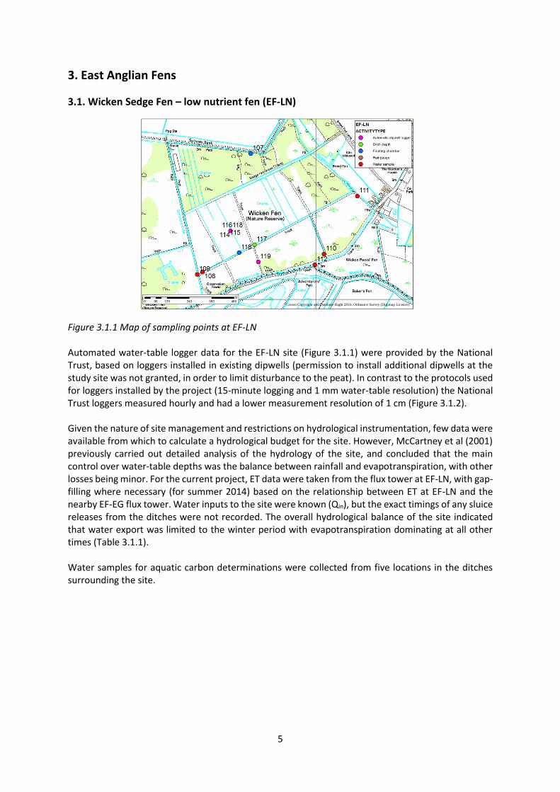
Figure 3.1.1 Map of sampling points at EF-LN Automated water-table logger data for the EF-LN site (Figure 3.1.1) were provided by the National Trust, based on loggers installed in existing dipwells (permission to install additional dipwells at the study site was not granted, in order to limit disturbance to the peat). In contrast to the protocols used for loggers installed by the project (15-minute logging and 1 mm water-table resolution) the National Trust loggers measured hourly and had a lower measurement resolution of 1 cm (Figure 3.1.2). Given the nature of site management and restrictions on hydrological instrumentation, few data were available from which to calculate a hydrological budget for the site. However, McCartney et al (2001) previously carried out detailed analysis of the hydrology of the site, and concluded that the main control over water-table depths was the balance between rainfall and evapotranspiration, with other losses being minor. For the current project, ET data were taken from the flux tower at EF-LN, with gap-filling where necessary (for summer 2014) based on the relationship between ET at EF-LN and the nearby EF-EG flux tower. Water inputs to the site were known (Qin), but the exact timings of any sluice releases from the ditches were not recorded. The overall hydrological balance of the site indicated that water export was limited to the winter period with evapotranspiration dominating at all other times (Table 3.1.1). Water samples for aquatic carbon determinations were collected from five locations in the ditches surrounding the site.

©Crown Copyright and Database Right 2016. Ordnance Survey (Digimap Licence)

6

Summary results

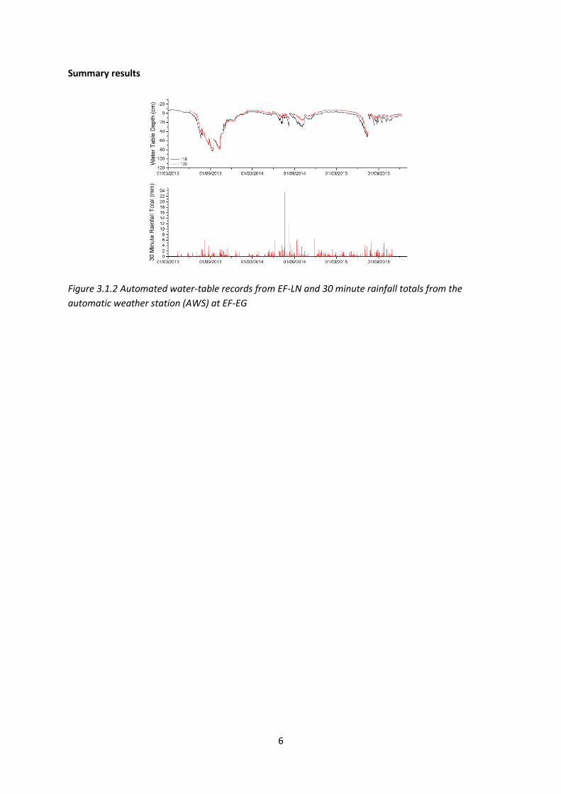
Figure 3.1.2 Automated water-table records from EF-LN and 30 minute rainfall totals from the

automatic weather station (AWS) at EF-EG

7

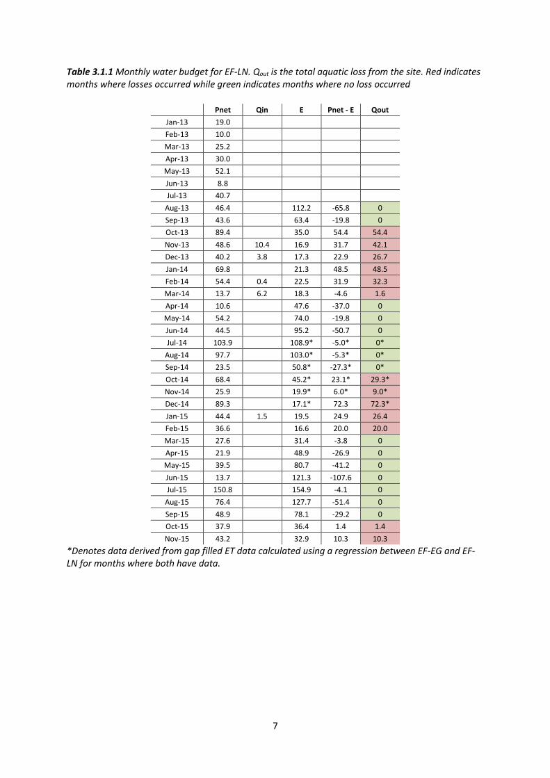
Table 3.1.1 Monthly water budget for EF-LN. Qout is the total aquatic loss from the site. Red indicates months where losses occurred while green indicates months where no loss occurred

Pnet Qin E Pnet - E Qout

Jan-13 19.0

Feb-13 10.0

Mar-13 25.2

Apr-13 30.0

May-13 52.1

Jun-13 8.8

Jul-13 40.7

Aug-13 46.4 112.2 -65.8 0

Sep-13 43.6 63.4 -19.8 0

Oct-13 89.4 35.0 54.4 54.4

Nov-13 48.6 10.4 16.9 31.7 42.1

Dec-13 40.2 3.8 17.3 22.9 26.7

Jan-14 69.8 21.3 48.5 48.5

Feb-14 54.4 0.4 22.5 31.9 32.3

Mar-14 13.7 6.2 18.3 -4.6 1.6

Apr-14 10.6 47.6 -37.0 0

May-14 54.2 74.0 -19.8 0

Jun-14 44.5 95.2 -50.7 0

Jul-14 103.9 108.9* -5.0* 0*

Aug-14 97.7 103.0* -5.3* 0*

Sep-14 23.5 50.8* -27.3* 0*

Oct-14 68.4 45.2* 23.1* 29.3*

Nov-14 25.9 19.9* 6.0* 9.0*

Dec-14 89.3 17.1* 72.3 72.3*

Jan-15 44.4 1.5 19.5 24.9 26.4

Feb-15 36.6 16.6 20.0 20.0

Mar-15 27.6 31.4 -3.8 0

Apr-15 21.9 48.9 -26.9 0

May-15 39.5 80.7 -41.2 0

Jun-15 13.7 121.3 -107.6 0

Jul-15 150.8 154.9 -4.1 0

Aug-15 76.4 127.7 -51.4 0

Sep-15 48.9 78.1 -29.2 0

Oct-15 37.9 36.4 1.4 1.4

Nov-15 43.2 32.9 10.3 10.3

*Denotes data derived from gap filled ET data calculated using a regression between EF-EG and EF-LN for months where both have data.

8

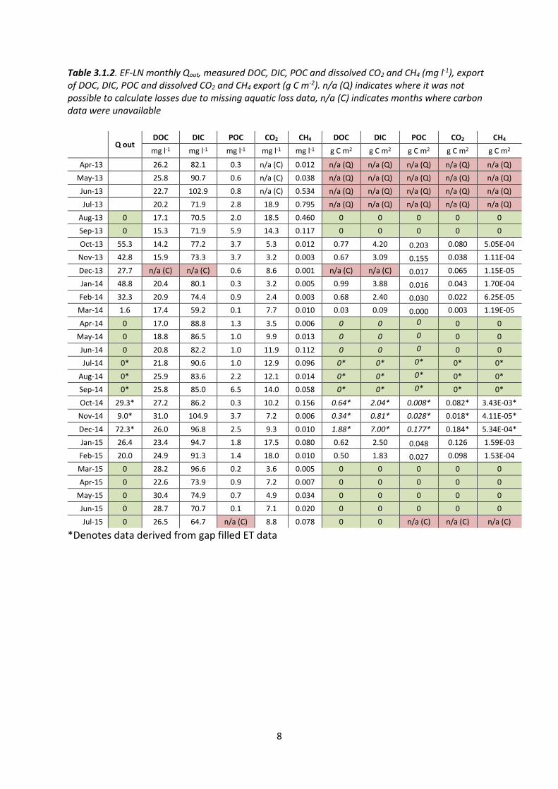
Table 3.1.2. EF-LN monthly Qout, measured DOC, DIC, POC and dissolved CO2 and CH4 (mg l-1), export of DOC, DIC, POC and dissolved CO2 and CH4 export (g C m-2). n/a (Q) indicates where it was not possible to calculate losses due to missing aquatic loss data, n/a (C) indicates months where carbon data were unavailable

Q out DOC DIC POC CO2 CH4 DOC DIC POC CO2 CH4

mg l-1 mg l-1 mg l-1 mg l-1 mg l-1 g C m2 g C m2 g C m2 g C m2 g C m2

Apr-13 26.2 82.1 0.3 n/a (C) 0.012 n/a (Q) n/a (Q) n/a (Q) n/a (Q) n/a (Q)

May-13 25.8 90.7 0.6 n/a (C) 0.038 n/a (Q) n/a (Q) n/a (Q) n/a (Q) n/a (Q)

Jun-13 22.7 102.9 0.8 n/a (C) 0.534 n/a (Q) n/a (Q) n/a (Q) n/a (Q) n/a (Q)

Jul-13 20.2 71.9 2.8 18.9 0.795 n/a (Q) n/a (Q) n/a (Q) n/a (Q) n/a (Q)

Aug-13 0 17.1 70.5 2.0 18.5 0.460 0 0 0 0 0

Sep-13 0 15.3 71.9 5.9 14.3 0.117 0 0 0 0 0

Oct-13 55.3 14.2 77.2 3.7 5.3 0.012 0.77 4.20 0.203 0.080 5.05E-04

Nov-13 42.8 15.9 73.3 3.7 3.2 0.003 0.67 3.09 0.155 0.038 1.11E-04

Dec-13 27.7 n/a (C) n/a (C) 0.6 8.6 0.001 n/a (C) n/a (C) 0.017 0.065 1.15E-05

Jan-14 48.8 20.4 80.1 0.3 3.2 0.005 0.99 3.88 0.016 0.043 1.70E-04

Feb-14 32.3 20.9 74.4 0.9 2.4 0.003 0.68 2.40 0.030 0.022 6.25E-05

Mar-14 1.6 17.4 59.2 0.1 7.7 0.010 0.03 0.09 0.000 0.003 1.19E-05

Apr-14 0 17.0 88.8 1.3 3.5 0.006 0 0 0 0 0

May-14 0 18.8 86.5 1.0 9.9 0.013 0 0 0 0 0

Jun-14 0 20.8 82.2 1.0 11.9 0.112 0 0 0 0 0

Jul-14 0* 21.8 90.6 1.0 12.9 0.096 0* 0* 0* 0* 0*

Aug-14 0* 25.9 83.6 2.2 12.1 0.014 0* 0* 0* 0* 0*

Sep-14 0* 25.8 85.0 6.5 14.0 0.058 0* 0* 0* 0* 0*

Oct-14 29.3* 27.2 86.2 0.3 10.2 0.156 0.64* 2.04* 0.008* 0.082* 3.43E-03*

Nov-14 9.0* 31.0 104.9 3.7 7.2 0.006 0.34* 0.81* 0.028* 0.018* 4.11E-05*

Dec-14 72.3* 26.0 96.8 2.5 9.3 0.010 1.88* 7.00* 0.177* 0.184* 5.34E-04*

Jan-15 26.4 23.4 94.7 1.8 17.5 0.080 0.62 2.50 0.048 0.126 1.59E-03

Feb-15 20.0 24.9 91.3 1.4 18.0 0.010 0.50 1.83 0.027 0.098 1.53E-04

Mar-15 0 28.2 96.6 0.2 3.6 0.005 0 0 0 0 0

Apr-15 0 22.6 73.9 0.9 7.2 0.007 0 0 0 0 0

May-15 0 30.4 74.9 0.7 4.9 0.034 0 0 0 0 0

Jun-15 0 28.7 70.7 0.1 7.1 0.020 0 0 0 0 0

Jul-15 0 26.5 64.7 n/a (C) 8.8 0.078 0 0 n/a (C) n/a (C) n/a (C)

*Denotes data derived from gap filled ET data

9

3.2. Bakers Fen – extensive grassland (EF-EG)

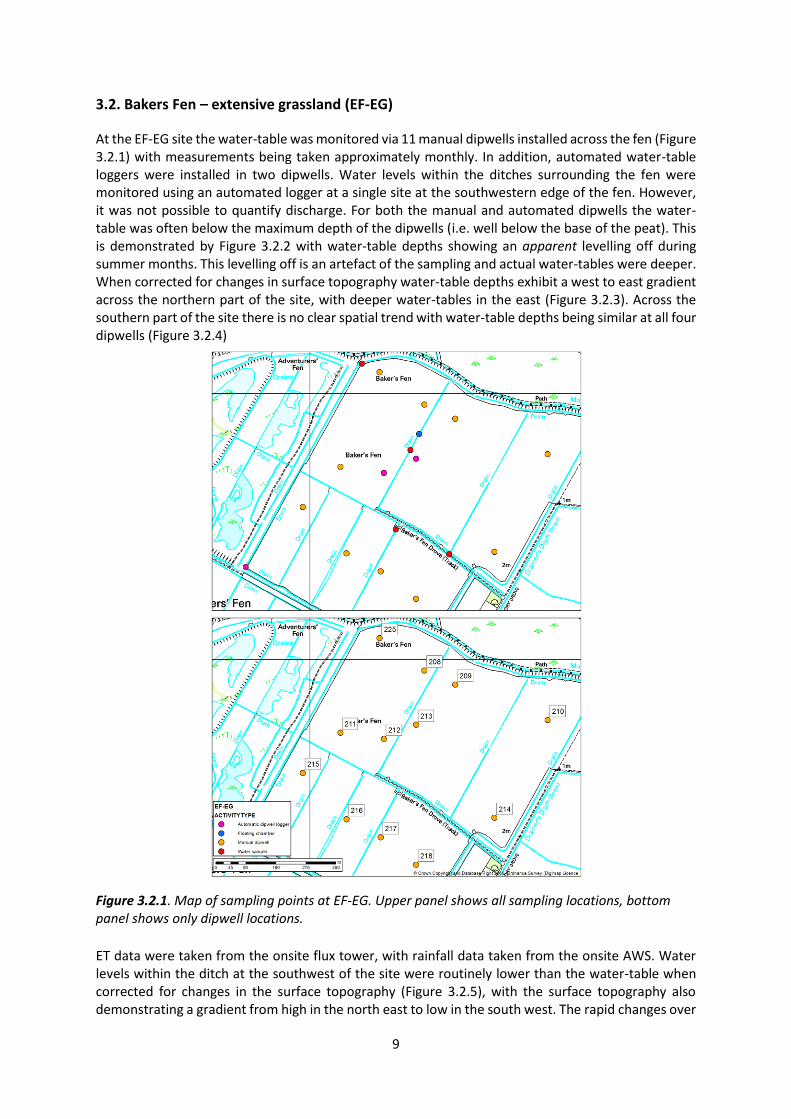
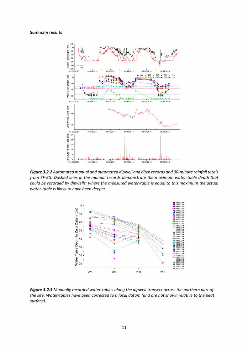
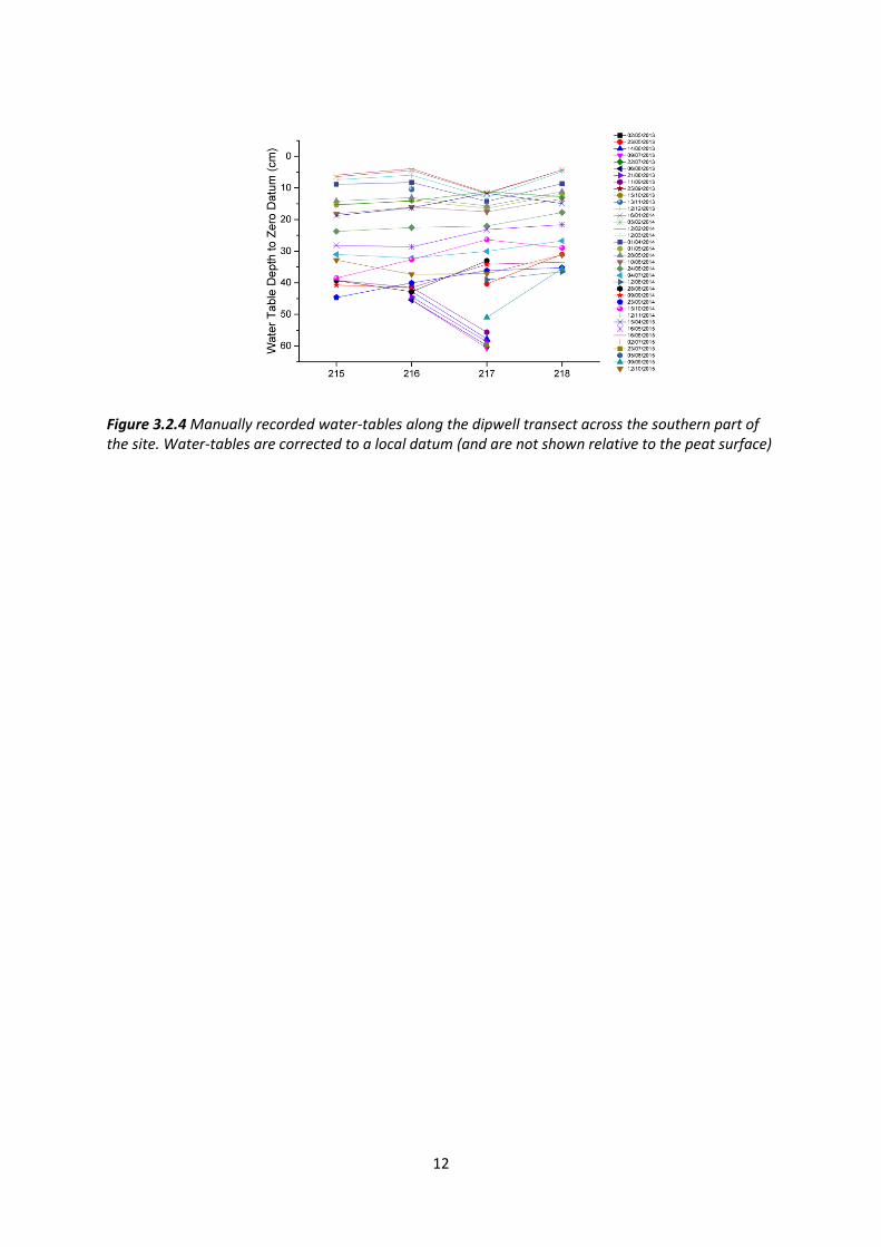
At the EF-EG site the water-table was monitored via 11 manual dipwells installed across the fen (Figure 3.2.1) with measurements being taken approximately monthly. In addition, automated water-table loggers were installed in two dipwells. Water levels within the ditches surrounding the fen were monitored using an automated logger at a single site at the southwestern edge of the fen. However, it was not possible to quantify discharge. For both the manual and automated dipwells the water-table was often below the maximum depth of the dipwells (i.e. well below the base of the peat). This is demonstrated by Figure 3.2.2 with water-table depths showing an apparent levelling off during summer months. This levelling off is an artefact of the sampling and actual water-tables were deeper. When corrected for changes in surface topography water-table depths exhibit a west to east gradient across the northern part of the site, with deeper water-tables in the east (Figure 3.2.3). Across the southern part of the site there is no clear spatial trend with water-table depths being similar at all four dipwells (Figure 3.2.4)

Figure 3.2.1. Map of sampling points at EF-EG. Upper panel shows all sampling locations, bottom panel shows only dipwell locations.

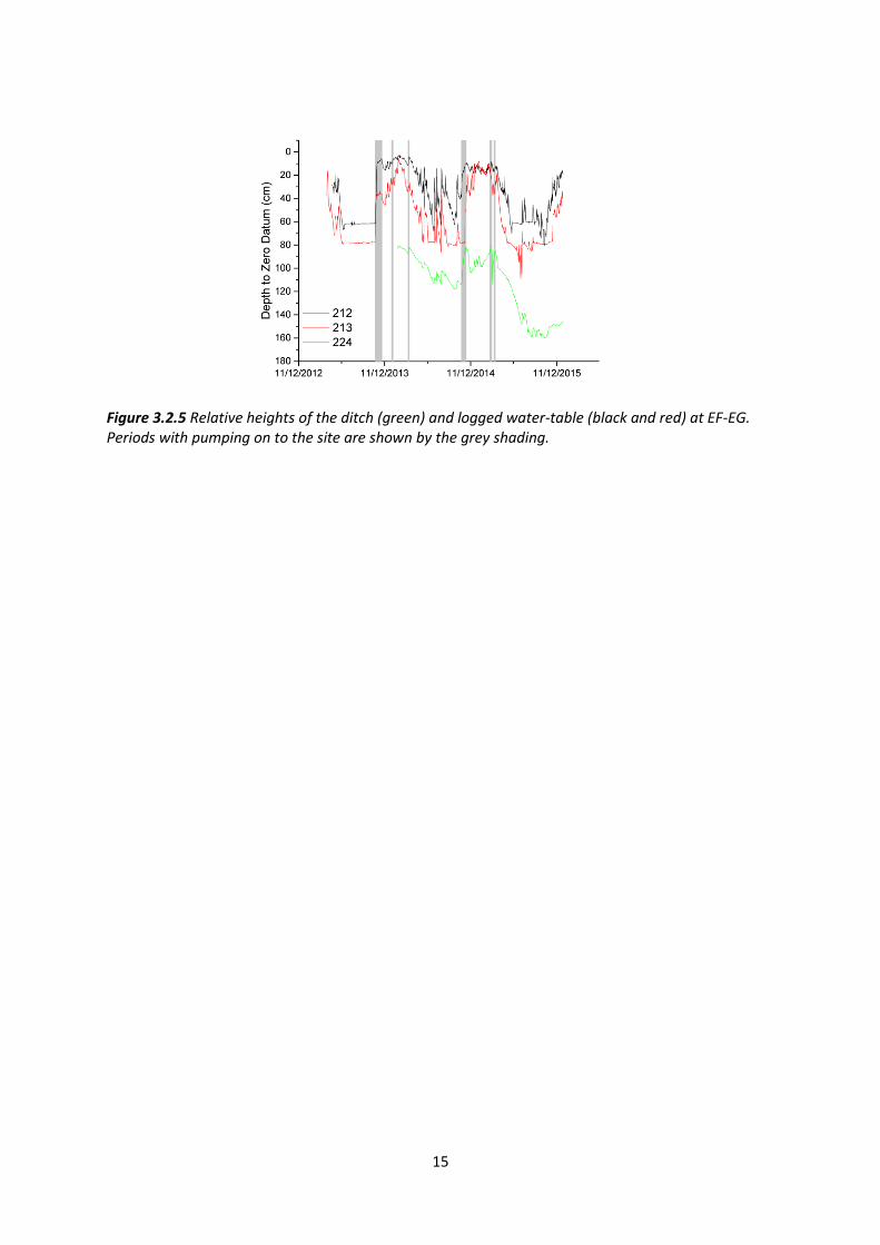
ET data were taken from the onsite flux tower, with rainfall data taken from the onsite AWS. Water levels within the ditch at the southwest of the site were routinely lower than the water-table when corrected for changes in the surface topography (Figure 3.2.5), with the surface topography also demonstrating a gradient from high in the north east to low in the south west. The rapid changes over

10

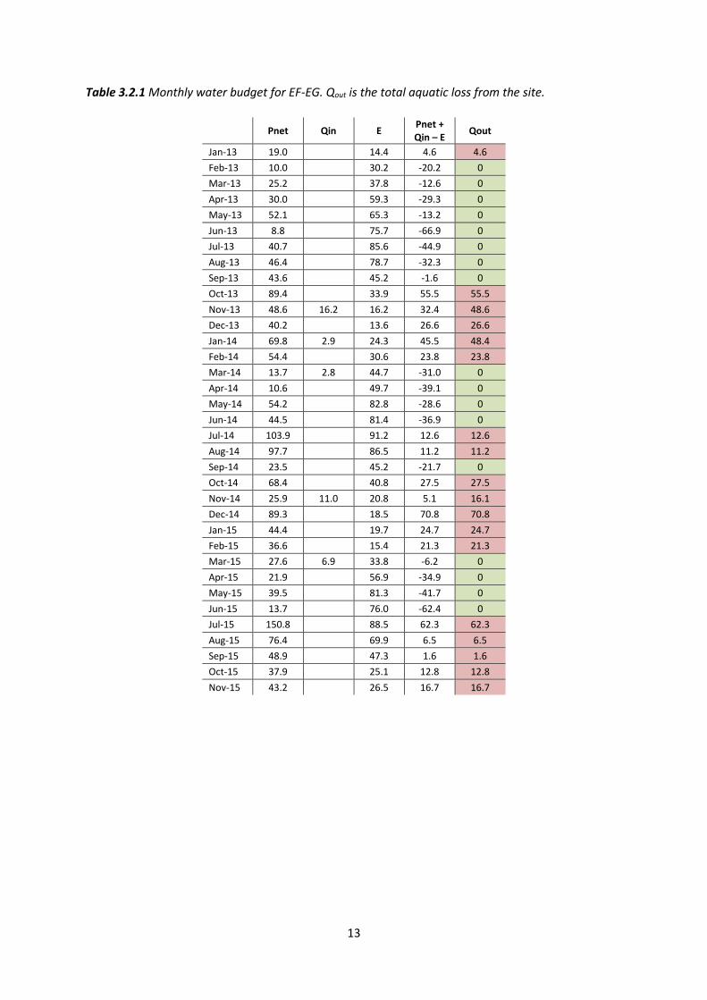
time in ditch water level heights at EF-EG supports the idea that they are controlled by water delivered from the fen rather than being used to support water levels within the fen. As such Qin is limited to water pumped on to the site during winter, the total volume of which is known (Table 3.2.1 and Figure 3.2.5). The overall hydrological balance of the site indicated that evapotranspiration dominates during spring and early summer, with no water export during this period (Table 3.2.2). During 2013 this period of dominance by evapotranspiration extended through to September. However, during 2014 and 2015 summer rainfall meant that this dominance ended earlier, with water export occurring from July onwards. During winter, when rainfall exceeds ET, water export occurs. Water quality samples were collected from four locations within the ditch network approximately monthly but sometimes fortnightly.

11

Summary results

Figure 3.2.2 Automated manual and automated dipwell and ditch records and 30-minute rainfall totals from EF-EG. Dashed lines in the manual records demonstrate the maximum water-table depth that could be recorded by dipwells: where the measured water-table is equal to this maximum the actual water-table is likely to have been deeper.

Figure 3.2.3 Manually recorded water-tables along the dipwell transect across the northern part of the site. Water-tables have been corrected to a local datum (and are not shown relative to the peat surface).

12

Figure 3.2.4 Manually recorded water-tables along the dipwell transect across the southern part of the site. Water-tables are corrected to a local datum (and are not shown relative to the peat surface)

13

Table 3.2.1 Monthly water budget for EF-EG. Qout is the total aquatic loss from the site.

Pnet Qin E Pnet + Qin – E

Qout

Jan-13 19.0 14.4 4.6 4.6

Feb-13 10.0 30.2 -20.2 0

Mar-13 25.2 37.8 -12.6 0

Apr-13 30.0 59.3 -29.3 0

May-13 52.1 65.3 -13.2 0

Jun-13 8.8 75.7 -66.9 0

Jul-13 40.7 85.6 -44.9 0

Aug-13 46.4 78.7 -32.3 0

Sep-13 43.6 45.2 -1.6 0

Oct-13 89.4 33.9 55.5 55.5

Nov-13 48.6 16.2 16.2 32.4 48.6

Dec-13 40.2 13.6 26.6 26.6

Jan-14 69.8 2.9 24.3 45.5 48.4

Feb-14 54.4 30.6 23.8 23.8

Mar-14 13.7 2.8 44.7 -31.0 0

Apr-14 10.6 49.7 -39.1 0

May-14 54.2 82.8 -28.6 0

Jun-14 44.5 81.4 -36.9 0

Jul-14 103.9 91.2 12.6 12.6

Aug-14 97.7 86.5 11.2 11.2

Sep-14 23.5 45.2 -21.7 0

Oct-14 68.4 40.8 27.5 27.5

Nov-14 25.9 11.0 20.8 5.1 16.1

Dec-14 89.3 18.5 70.8 70.8

Jan-15 44.4 19.7 24.7 24.7

Feb-15 36.6 15.4 21.3 21.3

Mar-15 27.6 6.9 33.8 -6.2 0

Apr-15 21.9 56.9 -34.9 0

May-15 39.5 81.3 -41.7 0

Jun-15 13.7 76.0 -62.4 0

Jul-15 150.8 88.5 62.3 62.3

Aug-15 76.4 69.9 6.5 6.5

Sep-15 48.9 47.3 1.6 1.6

Oct-15 37.9 25.1 12.8 12.8

Nov-15 43.2 26.5 16.7 16.7

14

Table 3.2.2 EF-EG monthly Qout, measured DOC, DIC, POC and dissolved CO2 and CH4 (mg l-1), export of DOC, DIC, POC and dissolved CO2 and CH4 g (g C m-2).

Q out

DOC DIC POC CO2 CH4 DOC DIC POC CO2 CH4


Apr-13 0 42.1 91.1 1.2 0.017 0 0 0 0 0

May-13 0 39.9 78.8 3.0 0.044 0 0 0 0 0

Jun-13 0 57.3 93.3 7.7 0.090 0 0 0 0 0

Jul-13 0 60.7 71.4 39.9 8.9 0.259 0 0 0 0 0

Aug-13 0 45.2 94.2 136.1 15.8 0.508 0 0 0 0 0

Sep-13 0 41.7 79.9 82.6 22.2 1.100 0 0 0 0 0

Oct-13 55.5 27.7 68.7 10.0 10.6 0.243 1.54 3.81 0.555 0.161 1.02E-02

Nov-13 48.6 9.9 62.8 2.0 4.6 0.011 0.48 3.05 0.096 0.060 4.05E-04

Dec-13 26.6 n/a (C) n/a (C) 1.2 n/a (C) n/a (C) n/a (C) n/a (C) 0.033 n/a (C) n/a (C)

Jan-14 48.4 13.5 53.3 0.5 5.2 0.009 0.65 2.58 0.022 0.068 3.38E-04

Feb-14 23.8 27.1 83.7 0.6 4.2 0.008 0.64 1.99 0.013 0.027 1.48E-04

Mar-14 0 46.6 89.5 0.9 4.6 0.010 0 0 0 0 0

Apr-14 0 36.1 95.0 5.0 3.0 0.006 0 0 0 0 0

May-14 0 33.8 105.0 1.0 5.7 0.032 0 0 0 0 0

Jun-14 0 33.7 96.4 8.3 4.3 0.021 0 0 0 0 0

Jul-14 12.6 36.6 130.1 n/a (C) 6.3 0.036 0.46 1.64 n/a (C) 0.022 3.37E-04

Aug-14 11.2 31.1 90.4 18.3 7.7 0.029 0.35 1.01 0.205 0.025 2.45E-04

Sep-14 0 26.6 99.6 8.8 7.7 0.029 0 0 0 0 0

Oct-14 27.5 23.6 84.1 5.1 8.1 0.355 0.65 2.31 0.140 0.060 7.33E-03

Nov-14 16.1 19.3 80.7 5.8 7.4 0.020 0.31 1.30 0.094 0.033 2.46E-04

Dec-14 70.8 22.1 100.7 1.2 9.7 0.016 1.56 7.13 0.081 0.185 8.80E-04

Jan-15 24.7 32.2 127.8 2.3 7.4 0.011 0.80 3.16 0.057 0.049 1.96E-04

Feb-15 21.3 29.8 117.3 6.8 9.2 0.011 0.63 2.50 0.144 0.054 1.77E-04

Mar-15 0.7 27.2 90.8 0.9 6.1 0.009 0.02 0.06 0.001 0.001 4.68E-06

Apr-15 0 25.9 82.6 0.6 4.6 0.015 0 0 0 0 0

May-15 0 48.4 82.5 1.4 3.9 0.011 0 0 0 0 0

Jun-15 0 49.8 85.0 2.4 4.4 0.027 0 0 0 0 0

Jul-15 62.3 44.0 73.1 n/a (C) 4.3 0.022 2.74 4.55 n/a (C) 0.074 1.02E-03

15

Figure 3.2.5 Relative heights of the ditch (green) and logged water-table (black and red) at EF-EG. Periods with pumping on to the site are shown by the grey shading.

16

3.3. Rosedene Farm – arable on deep peat (EF-DA)

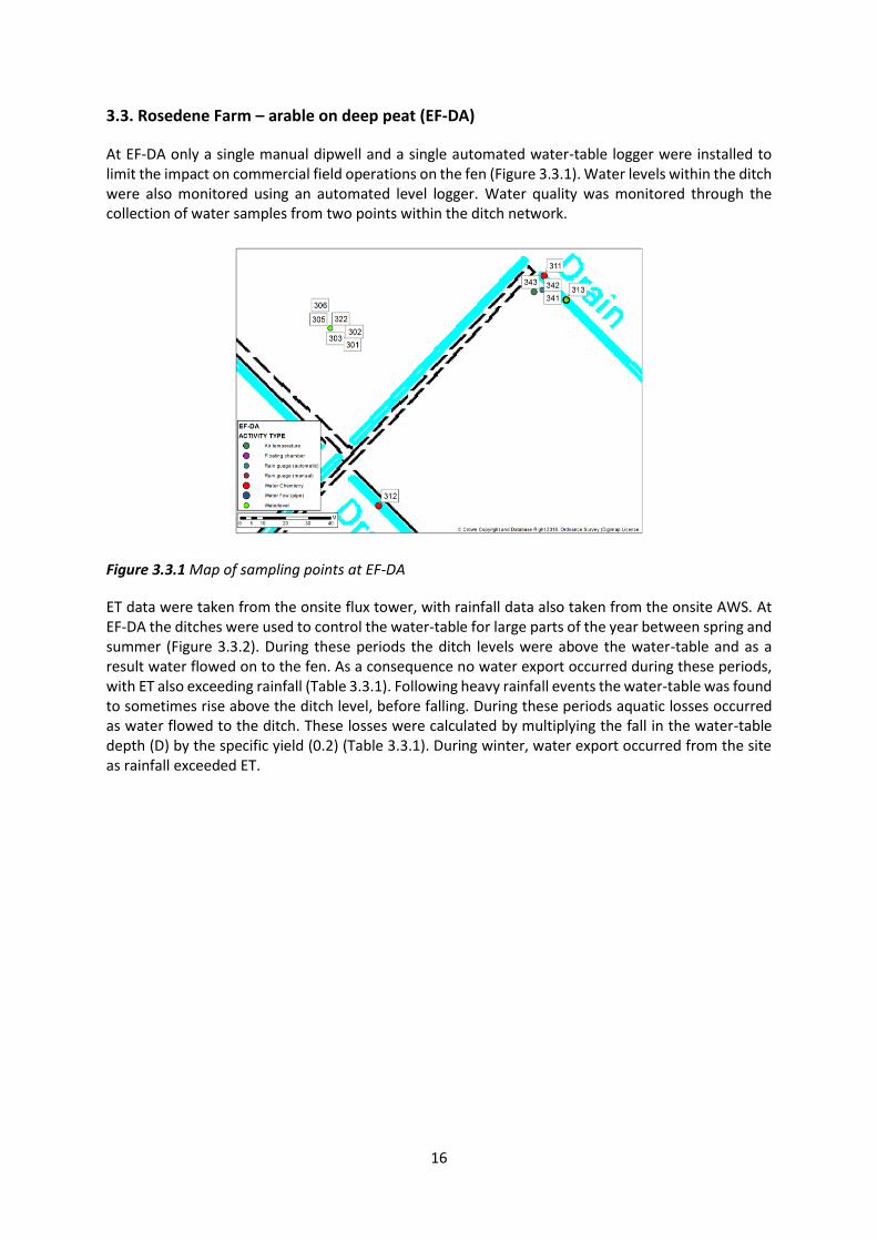
At EF-DA only a single manual dipwell and a single automated water-table logger were installed to limit the impact on commercial field operations on the fen (Figure 3.3.1). Water levels within the ditch were also monitored using an automated level logger. Water quality was monitored through the collection of water samples from two points within the ditch network.

Figure 3.3.1 Map of sampling points at EF-DA

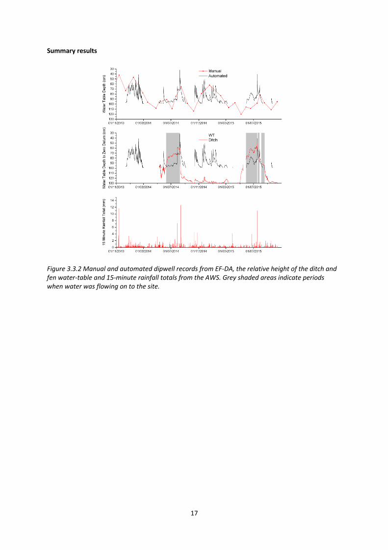
ET data were taken from the onsite flux tower, with rainfall data also taken from the onsite AWS. At EF-DA the ditches were used to control the water-table for large parts of the year between spring and summer (Figure 3.3.2). During these periods the ditch levels were above the water-table and as a result water flowed on to the fen. As a consequence no water export occurred during these periods, with ET also exceeding rainfall (Table 3.3.1). Following heavy rainfall events the water-table was found to sometimes rise above the ditch level, before falling. During these periods aquatic losses occurred as water flowed to the ditch. These losses were calculated by multiplying the fall in the water-table depth (D) by the specific yield (0.2) (Table 3.3.1). During winter, water export occurred from the site as rainfall exceeded ET.

17

Summary results

Figure 3.3.2 Manual and automated dipwell records from EF-DA, the relative height of the ditch and fen water-table and 15-minute rainfall totals from the AWS. Grey shaded areas indicate periods when water was flowing on to the site.

18

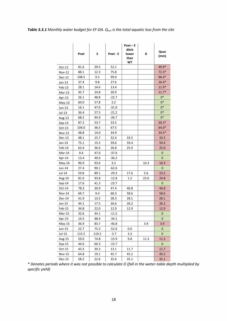
Table 3.3.1 Monthly water budget for EF-DA. Qout is the total aquatic loss from the site

Pnet E Pnet - E

Pnet – E ditch lower than WT

D Qout (mm)

Oct-12 81.6 29.5 52.1 49.9*

Nov-12 88.1 12.3 75.8 72.3*

Dec-12 108.5 9.5 99.0 96.6*

Jan-13 37.4 9.8 27.6 26.4*

Feb-13 28.1 14.6 13.4 11.9*

Mar-13 45.7 24.8 20.9 11.7*

Apr-13 26.1 48.8 -22.7 0*

May-13 60.0 57.8 2.2 0*

Jun-13 16.1 47.0 -31.0 0*

Jul-13 36.4 57.5 -21.2 0*

Aug-13 68.2 94.9 -26.7 0*

Sep-13 87.2 53.7 33.5 30.3*

Oct-13 104.0 36.5 67.5 64.0*

Nov-13 48.8 14.0 34.9 34.5*

Dec-13 48.1 15.7 32.4 33.5 33.5

Jan-14 75.1 15.5 59.6 59.4 59.4

Feb-14 63.4 36.6 26.8 25.0 25.0

Mar-14 9.4 47.0 -37.6 0

Apr-14 13.4 49.6 -36.2 0

May-14 96.9 93.6 3.3 10.3 10.3

Jun-14 27.4 90.1 -62.6 0

Jul-14 59.8 89.1 -29.3 17.6 5.6 23.2

Aug-14 81.0 93.8 -12.8 1.2 23.6 24.8

Sep-14 17.6 41.3 -23.7 0

Oct-14 78.3 30.9 47.4 46.8 46.8

Nov-14 69.7 9.4 60.3 58.6 58.6

Dec-14 41.9 13.5 28.3 28.1 28.1

Jan-15 44.1 17.5 26.6 26.2 26.2

Feb-15 34.8 22.0 12.9 12.9 12.9

Mar-15 32.6 44.1 -11.5 0

Apr-15 14.3 48.4 -34.1 0

May-15 36.9 83.7 -46.8 3.9 3.9

Jun-15 22.7 75.3 -52.6 0.0 0

Jul-15 115.5 119.2 -3.7 3.3 0

Aug-15 59.0 74.8 -15.9 9.8 11.3 11.3

Sep-15 44.6 60.3 -15.7 0

Oct-15 43.3 30.3 13.1 11.7 11.7

Nov-15 64.8 19.1 45.7 45.2 45.2

Dec-15 58.2 22.6 35.6 35.1 35.1

* Denotes periods where it was not possible to calculate D (fall in the water-table depth multiplied by specific yield)

19

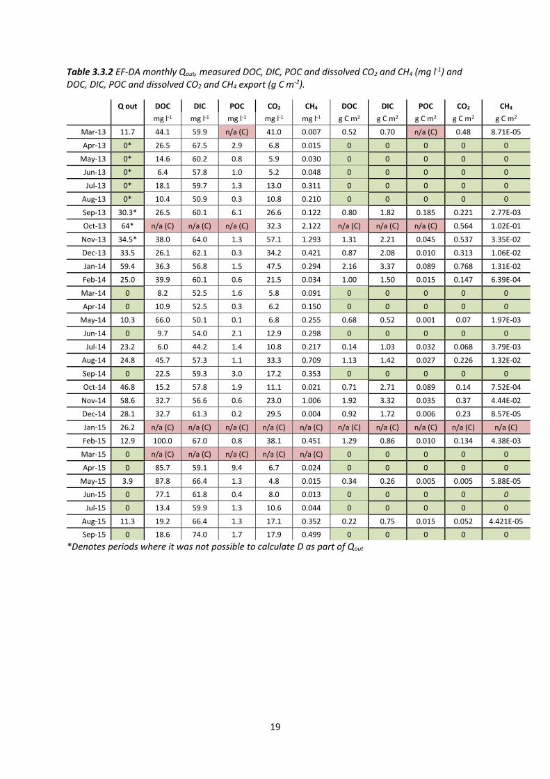
Table 3.3.2 EF-DA monthly Qout, measured DOC, DIC, POC and dissolved CO2 and CH4 (mg l-1) and DOC, DIC, POC and dissolved CO2 and CH4 export (g C m-2).



Mar-13 11.7 44.1 59.9 n/a (C) 41.0 0.007 0.52 0.70 n/a (C) 0.48 8.71E-05

Apr-13 0* 26.5 67.5 2.9 6.8 0.015 0 0 0 0 0

May-13 0* 14.6 60.2 0.8 5.9 0.030 0 0 0 0 0

Jun-13 0* 6.4 57.8 1.0 5.2 0.048 0 0 0 0 0

Jul-13 0* 18.1 59.7 1.3 13.0 0.311 0 0 0 0 0

Aug-13 0* 10.4 50.9 0.3 10.8 0.210 0 0 0 0 0

Sep-13 30.3* 26.5 60.1 6.1 26.6 0.122 0.80 1.82 0.185 0.221 2.77E-03

Oct-13 64* n/a (C) n/a (C) n/a (C) 32.3 2.122 n/a (C) n/a (C) n/a (C) 0.564 1.02E-01

Nov-13 34.5* 38.0 64.0 1.3 57.1 1.293 1.31 2.21 0.045 0.537 3.35E-02

Dec-13 33.5 26.1 62.1 0.3 34.2 0.421 0.87 2.08 0.010 0.313 1.06E-02

Jan-14 59.4 36.3 56.8 1.5 47.5 0.294 2.16 3.37 0.089 0.768 1.31E-02

Feb-14 25.0 39.9 60.1 0.6 21.5 0.034 1.00 1.50 0.015 0.147 6.39E-04

Mar-14 0 8.2 52.5 1.6 5.8 0.091 0 0 0 0 0

Apr-14 0 10.9 52.5 0.3 6.2 0.150 0 0 0 0 0

May-14 10.3 66.0 50.1 0.1 6.8 0.255 0.68 0.52 0.001 0.07 1.97E-03

Jun-14 0 9.7 54.0 2.1 12.9 0.298 0 0 0 0 0

Jul-14 23.2 6.0 44.2 1.4 10.8 0.217 0.14 1.03 0.032 0.068 3.79E-03

Aug-14 24.8 45.7 57.3 1.1 33.3 0.709 1.13 1.42 0.027 0.226 1.32E-02

Sep-14 0 22.5 59.3 3.0 17.2 0.353 0 0 0 0 0

Oct-14 46.8 15.2 57.8 1.9 11.1 0.021 0.71 2.71 0.089 0.14 7.52E-04

Nov-14 58.6 32.7 56.6 0.6 23.0 1.006 1.92 3.32 0.035 0.37 4.44E-02

Dec-14 28.1 32.7 61.3 0.2 29.5 0.004 0.92 1.72 0.006 0.23 8.57E-05

Jan-15 26.2 n/a (C) n/a (C) n/a (C) n/a (C) n/a (C) n/a (C) n/a (C) n/a (C) n/a (C) n/a (C)

Feb-15 12.9 100.0 67.0 0.8 38.1 0.451 1.29 0.86 0.010 0.134 4.38E-03

Mar-15 0 n/a (C) n/a (C) n/a (C) n/a (C) n/a (C) 0 0 0 0 0

Apr-15 0 85.7 59.1 9.4 6.7 0.024 0 0 0 0 0

May-15 3.9 87.8 66.4 1.3 4.8 0.015 0.34 0.26 0.005 0.005 5.88E-05

Jun-15 0 77.1 61.8 0.4 8.0 0.013 0 0 0 0 0

Jul-15 0 13.4 59.9 1.3 10.6 0.044 0 0 0 0 0

Aug-15 11.3 19.2 66.4 1.3 17.1 0.352 0.22 0.75 0.015 0.052 4.421E-05

Sep-15 0 18.6 74.0 1.7 17.9 0.499 0 0 0 0 0

*Denotes periods where it was not possible to calculate D as part of Qout

20

3.4. Redmere Farm – arable on shallow peat (EF-SA)

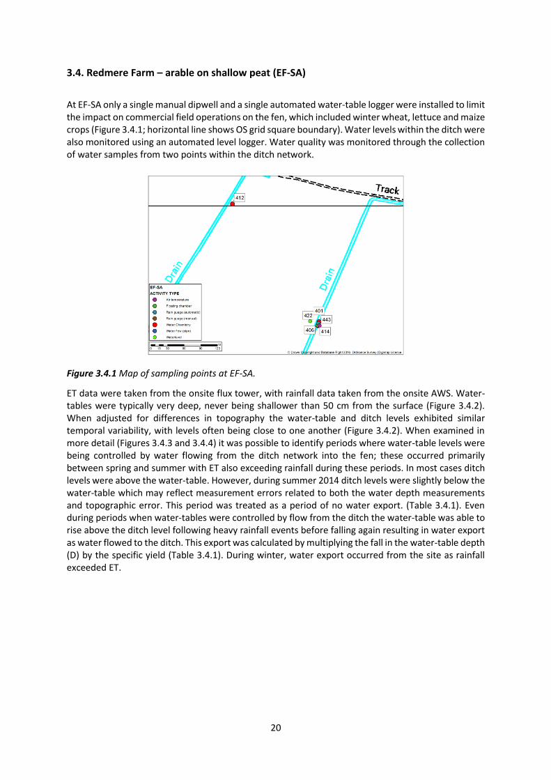
At EF-SA only a single manual dipwell and a single automated water-table logger were installed to limit the impact on commercial field operations on the fen, which included winter wheat, lettuce and maize crops (Figure 3.4.1; horizontal line shows OS grid square boundary). Water levels within the ditch were also monitored using an automated level logger. Water quality was monitored through the collection of water samples from two points within the ditch network.

Figure 3.4.1 Map of sampling points at EF-SA.

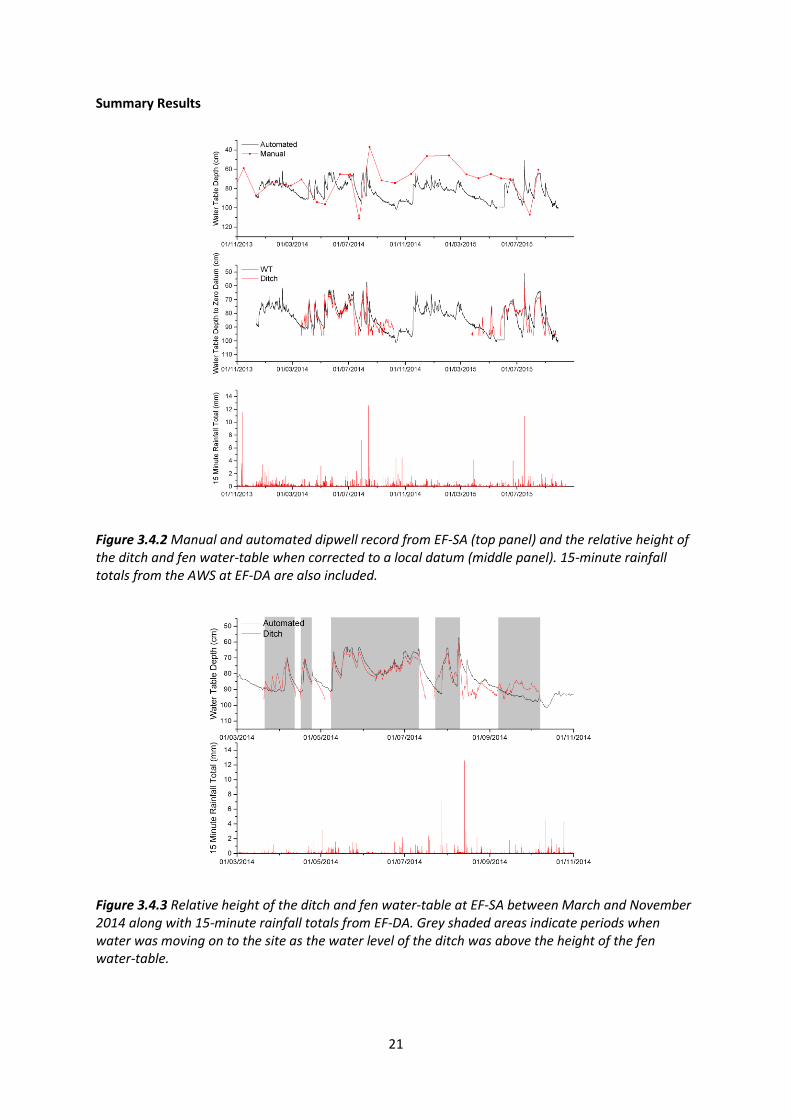
ET data were taken from the onsite flux tower, with rainfall data taken from the onsite AWS. Water-tables were typically very deep, never being shallower than 50 cm from the surface (Figure 3.4.2). When adjusted for differences in topography the water-table and ditch levels exhibited similar temporal variability, with levels often being close to one another (Figure 3.4.2). When examined in more detail (Figures 3.4.3 and 3.4.4) it was possible to identify periods where water-table levels were being controlled by water flowing from the ditch network into the fen; these occurred primarily between spring and summer with ET also exceeding rainfall during these periods. In most cases ditch levels were above the water-table. However, during summer 2014 ditch levels were slightly below the water-table which may reflect measurement errors related to both the water depth measurements and topographic error. This period was treated as a period of no water export. (Table 3.4.1). Even during periods when water-tables were controlled by flow from the ditch the water-table was able to rise above the ditch level following heavy rainfall events before falling again resulting in water export as water flowed to the ditch. This export was calculated by multiplying the fall in the water-table depth (D) by the specific yield (Table 3.4.1). During winter, water export occurred from the site as rainfall exceeded ET.

21

Summary Results

Figure 3.4.2 Manual and automated dipwell record from EF-SA (top panel) and the relative height of the ditch and fen water-table when corrected to a local datum (middle panel). 15-minute rainfall totals from the AWS at EF-DA are also included.

Figure 3.4.3 Relative height of the ditch and fen water-table at EF-SA between March and November 2014 along with 15-minute rainfall totals from EF-DA. Grey shaded areas indicate periods when water was moving on to the site as the water level of the ditch was above the height of the fen water-table.

22

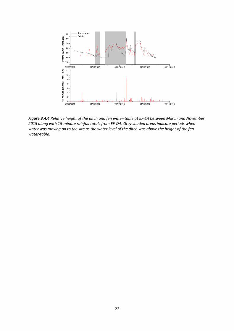
Figure 3.4.4 Relative height of the ditch and fen water-table at EF-SA between March and November 2015 along with 15-minute rainfall totals from EF-DA. Grey shaded areas indicate periods when water was moving on to the site as the water level of the ditch was above the height of the fen water-table.

23

Table 3.4.1 Monthly water budget for EF-SA. Qout is the total aquatic loss from the site.

Pnet E Pnet - E D Qout

Oct-12 41.0 13.7 27.3 27.3*

Nov-12 88.1 20.8 67.3 67.3*

Dec-12 108.5 15.5 93.0 93.0*

Jan-13 37.4 16.2 21.2 21.2*

Feb-13 28.1 24.5 3.6 3.6*

Mar-13 45.7 40.5 5.2 5.2*

Apr-13 26.1 72.6 -46.5 0*

May-13 60.0 100.9 -40.9 0*

Jun-13 16.1 107.6 -91.6 0*

Jul-13 36.4 125.9 -89.6 0*

Aug-13 68.2 74.8 -6.6 0*

Sep-13 87.2 43.4 43.8 43.8*

Oct-13 104.0 38.3 65.7 65.7*

Nov-13 48.8 23.5 25.3 25.3*

Dec-13 48.1 19.6 28.5 28.5

Jan-14 75.1 22.9 52.2 52.2

Feb-14 63.4 38.1 25.3 25.3

Mar-14 9.4 35.0 -25.6 0

Apr-14 13.4 46.9 -33.6 20.2 0

May-14 96.9 112.4 -15.5 0

Jun-14 27.4 111.9 -84.5 0

Jul-14 59.8 121.5 -61.7 12.6 12.6

Aug-14 81.0 119.3 -38.3 11.2 11.2

Sep-14 17.6 59.1 -41.5 0

Oct-14 78.3 47.3 30.9 2.9 33.8

Nov-14 69.7 17.1 52.7 52.7

Dec-14 41.9 20.7 21.1 21.1

Jan-15 44.1 25.4 18.7 18.7

Feb-15 34.8 25.9 9.0 9.0

Mar-15 32.6 54.7 -22.2 0

Apr-15 14.3 64.0 -49.7 0

May-15 36.9 91.2 -54.3 0

Jun-15 22.7 72.4 -49.7 0

Jul-15 115.5 99.8 15.7 13.7 29.4

Aug-15 59.0 103.7 -44.7 0.8 0.8

Sep-15 44.6 74.7 -30.1 0

Oct-15 43.3 36.8 6.6 6.6

Nov-15 64.8 30.6 34.2 34.2

Dec-15 58.2 27.4 30.8 30.8

*Denotes periods where it was not possible to calculate D as part of Qout

24

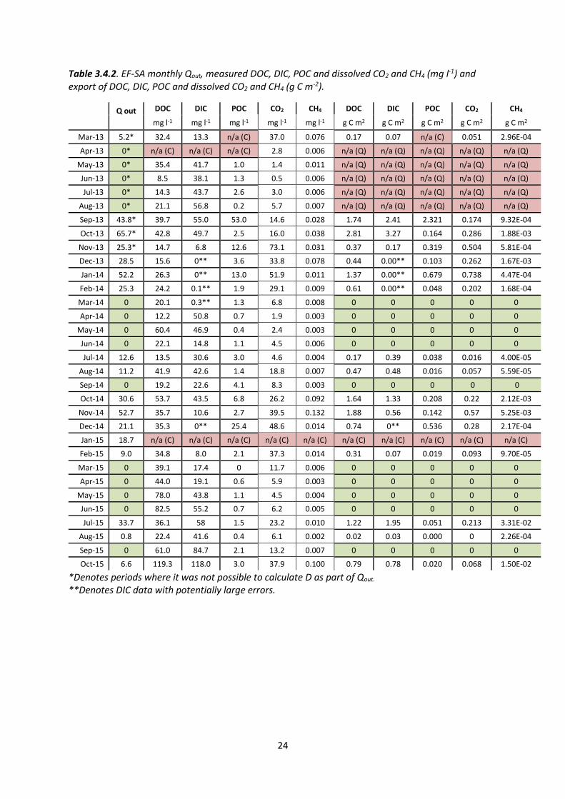
Table 3.4.2. EF-SA monthly Qout, measured DOC, DIC, POC and dissolved CO2 and CH4 (mg l-1) and export of DOC, DIC, POC and dissolved CO2 and CH4 (g C m-2).

*Denotes periods where it was not possible to calculate D as part of Qout. **Denotes DIC data with potentially large errors.

Q out



Mar-13 5.2* 32.4 13.3 n/a (C) 37.0 0.076 0.17 0.07 n/a (C) 0.051 2.96E-04

Apr-13 0* n/a (C) n/a (C) n/a (C) 2.8 0.006 n/a (Q) n/a (Q) n/a (Q) n/a (Q) n/a (Q)

May-13 0* 35.4 41.7 1.0 1.4 0.011 n/a (Q) n/a (Q) n/a (Q) n/a (Q) n/a (Q)

Jun-13 0* 8.5 38.1 1.3 0.5 0.006 n/a (Q) n/a (Q) n/a (Q) n/a (Q) n/a (Q)

Jul-13 0* 14.3 43.7 2.6 3.0 0.006 n/a (Q) n/a (Q) n/a (Q) n/a (Q) n/a (Q)

Aug-13 0* 21.1 56.8 0.2 5.7 0.007 n/a (Q) n/a (Q) n/a (Q) n/a (Q) n/a (Q)

Sep-13 43.8* 39.7 55.0 53.0 14.6 0.028 1.74 2.41 2.321 0.174 9.32E-04

Oct-13 65.7* 42.8 49.7 2.5 16.0 0.038 2.81 3.27 0.164 0.286 1.88E-03

Nov-13 25.3* 14.7 6.8 12.6 73.1 0.031 0.37 0.17 0.319 0.504 5.81E-04

Dec-13 28.5 15.6 0** 3.6 33.8 0.078 0.44 0.00** 0.103 0.262 1.67E-03

Jan-14 52.2 26.3 0** 13.0 51.9 0.011 1.37 0.00** 0.679 0.738 4.47E-04

Feb-14 25.3 24.2 0.1** 1.9 29.1 0.009 0.61 0.00** 0.048 0.202 1.68E-04

Mar-14 0 20.1 0.3** 1.3 6.8 0.008 0 0 0 0 0

Apr-14 0 12.2 50.8 0.7 1.9 0.003 0 0 0 0 0

May-14 0 60.4 46.9 0.4 2.4 0.003 0 0 0 0 0

Jun-14 0 22.1 14.8 1.1 4.5 0.006 0 0 0 0 0

Jul-14 12.6 13.5 30.6 3.0 4.6 0.004 0.17 0.39 0.038 0.016 4.00E-05

Aug-14 11.2 41.9 42.6 1.4 18.8 0.007 0.47 0.48 0.016 0.057 5.59E-05

Sep-14 0 19.2 22.6 4.1 8.3 0.003 0 0 0 0 0

Oct-14 30.6 53.7 43.5 6.8 26.2 0.092 1.64 1.33 0.208 0.22 2.12E-03

Nov-14 52.7 35.7 10.6 2.7 39.5 0.132 1.88 0.56 0.142 0.57 5.25E-03

Dec-14 21.1 35.3 0** 25.4 48.6 0.014 0.74 0** 0.536 0.28 2.17E-04


Feb-15 9.0 34.8 8.0 2.1 37.3 0.014 0.31 0.07 0.019 0.093 9.70E-05

Mar-15 0 39.1 17.4 0 11.7 0.006 0 0 0 0 0

Apr-15 0 44.0 19.1 0.6 5.9 0.003 0 0 0 0 0

May-15 0 78.0 43.8 1.1 4.5 0.004 0 0 0 0 0

Jun-15 0 82.5 55.2 0.7 6.2 0.005 0 0 0 0 0

Jul-15 33.7 36.1 58 1.5 23.2 0.010 1.22 1.95 0.051 0.213 3.31E-02

Aug-15 0.8 22.4 41.6 0.4 6.1 0.002 0.02 0.03 0.000 0 2.26E-04

Sep-15 0 61.0 84.7 2.1 13.2 0.007 0 0 0 0 0

Oct-15 6.6 119.3 118.0 3.0 37.9 0.100 0.79 0.78 0.020 0.068 1.50E-02

25

4. Manchester Mosses

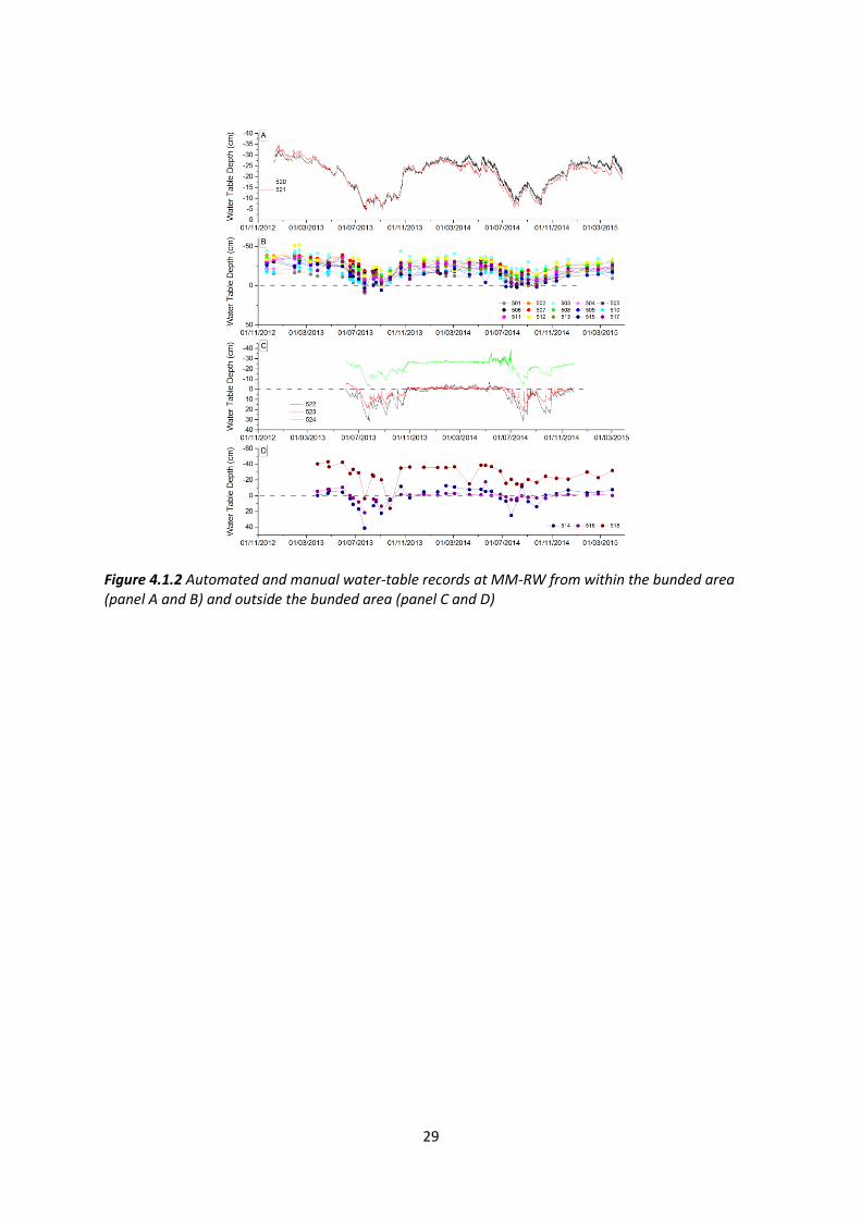
4.1. Astley Moss – Re-wetted raised bog (MM-RW)

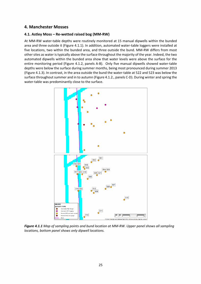
At MM-RW water-table depths were routinely monitored at 15 manual dipwells within the bunded area and three outside it (Figure 4.1.1). In addition, automated water-table loggers were installed at five locations, two within the bunded area, and three outside the bund. MM-RW differs from most other sites as water is typically above the surface throughout the majority of the year. Indeed, the two automated dipwells within the bunded area show that water levels were above the surface for the entire monitoring period (Figure 4.1.2, panels A-B). Only five manual dipwells showed water-table depths were below the surface during summer months, being most pronounced during summer 2013 (Figure 4.1.3). In contrast, in the area outside the bund the water-table at 522 and 523 was below the surface throughout summer and in to autumn (Figure 4.1.2., panels C-D). During winter and spring the water-table was predominantly close to the surface.

Figure 4.1.1 Map of sampling points and bund location at MM-RW. Upper panel shows all sampling locations, bottom panel shows only dipwell locations.

26

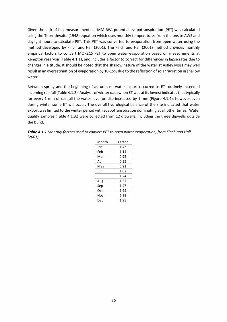
Given the lack of flux measurements at MM-RW, potential evapotranspiration (PET) was calculated

using the Thornthwaite (1948) equation which uses monthly temperatures from the onsite AWS and

daylight hours to calculate PET. This PET was converted to evaporation from open water using the

method developed by Finch and Hall (2001). The Finch and Hall (2001) method provides monthly

empirical factors to convert MORECS PET to open water evaporation based on measurements at

Kempton reservoir (Table 4.1.1), and includes a factor to correct for differences in lapse rates due to

changes in altitude. It should be noted that the shallow nature of the water at Astley Moss may well

result in an overestimation of evaporation by 10-15% due to the reflection of solar radiation in shallow

water.

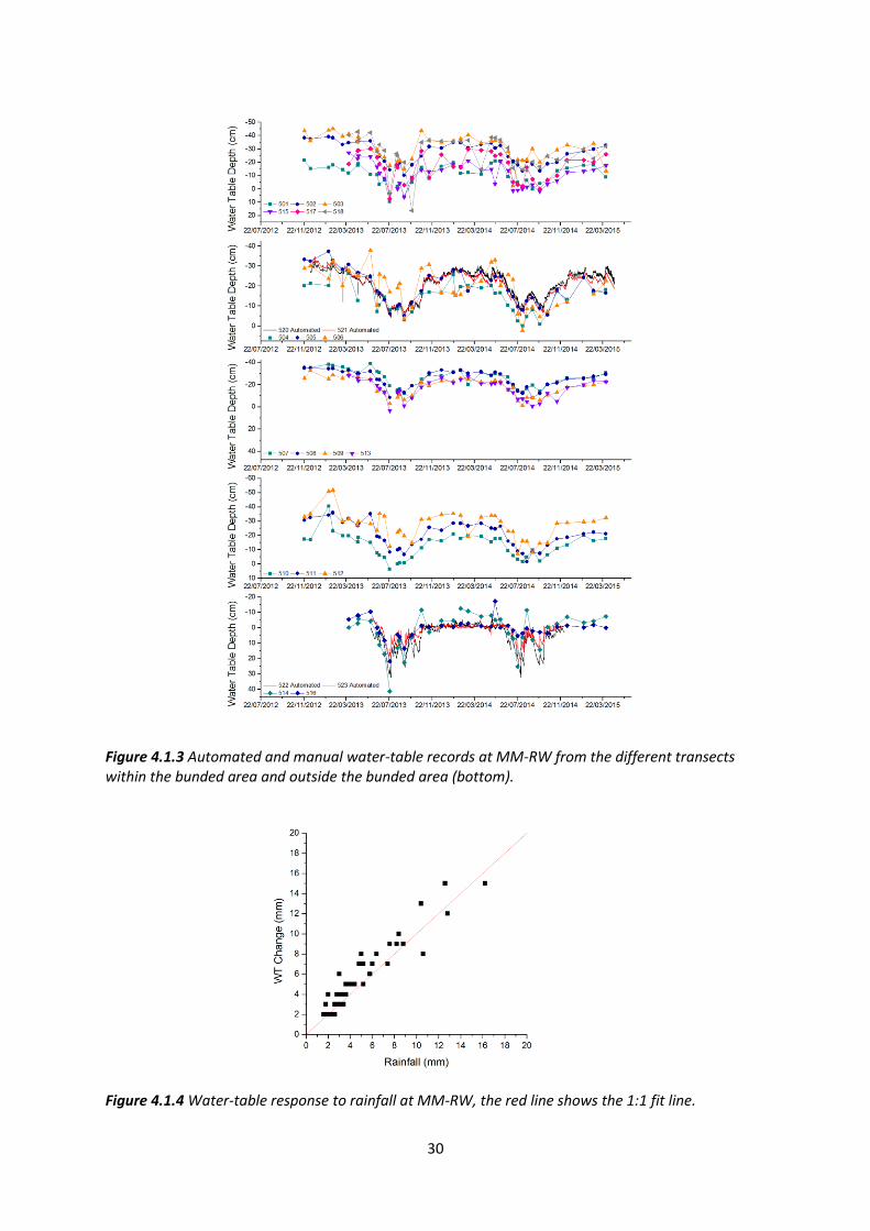
Between spring and the beginning of autumn no water export occurred as ET routinely exceeded

incoming rainfall (Table 4.1.2). Analysis of winter data when ET was at its lowest indicates that typically

for every 1 mm of rainfall the water level on site increased by 1 mm (Figure 4.1.4); however even

during winter some ET will occur. The overall hydrological balance of the site indicated that water

export was limited to the winter period with evapotranspiration dominating at all other times. Water

quality samples (Table 4.1.3.) were collected from 12 dipwells, including the three dipwells outside

the bund.

Table 4.1.1 Monthly factors used to convert PET to open water evaporation, from Finch and Hall (2001)

Month Factor

Jan 1.43

Feb 1.14

Mar 0.92

Apr 0.95

May 0.91

Jun 1.02

Jul 1.24

Aug 1.37

Sep 1.47

Oct 1.99

Nov 2.29

Dec 1.95

27

Table 4.1.2 Monthly water budget for MM-RW. Qout is the total aquatic loss from the site.

Pnet E (PET) Pnet - E Q out

Jan-13 59.8 18.5 41.3 41.3

Feb-13 59.4 17.8 41.6 41.6

Mar-13 43.8 34.8 9.0 9.0

Apr-13 25.4 55.3 -29.9 0

May-13 60.2 73.9 -13.7 0

Jun-13 45.0 86.4 -41.4 0

Jul-13 60.6 106.5 -45.9 0

Aug-13 65.4 92.0 -26.6 0

Sep-13 63.0 69.0 -6.0 0

Oct-13 139.0 52.3 86.7 86.7

Nov-13 89.0 34.6 54.4 54.4

Dec-13 70.0 18.9 51.1 51.1

Jan-14 66.0 18.5 47.5 47.5

Feb-14 80.4 17.8 62.6 62.6

Mar-14 58.8 34.8 24.0 24.0

Apr-14 49.8 55.3 -5.5 0

May-14 106 73.9 32.1 32.1

Jun-14 41.4 86.4 -45.0 0

Jul-14 45.2 106.5 -61.3 0

Aug-14 131.8 92.0 39.8 39.8

Sep-14 17.0 69.0 -52.0 0

Oct-14 88.6 52.3 36.3 36.3

Nov-14 61.0 34.6 26.4 26.4

Dec-14 111.2 18.9 92.3 92.3

Jan-15 104.8 18.5 86.3 86.3

Feb-15 46.2 17.8 28.4 28.4

Mar-15 88.2 34.8 53.4 53.4

28

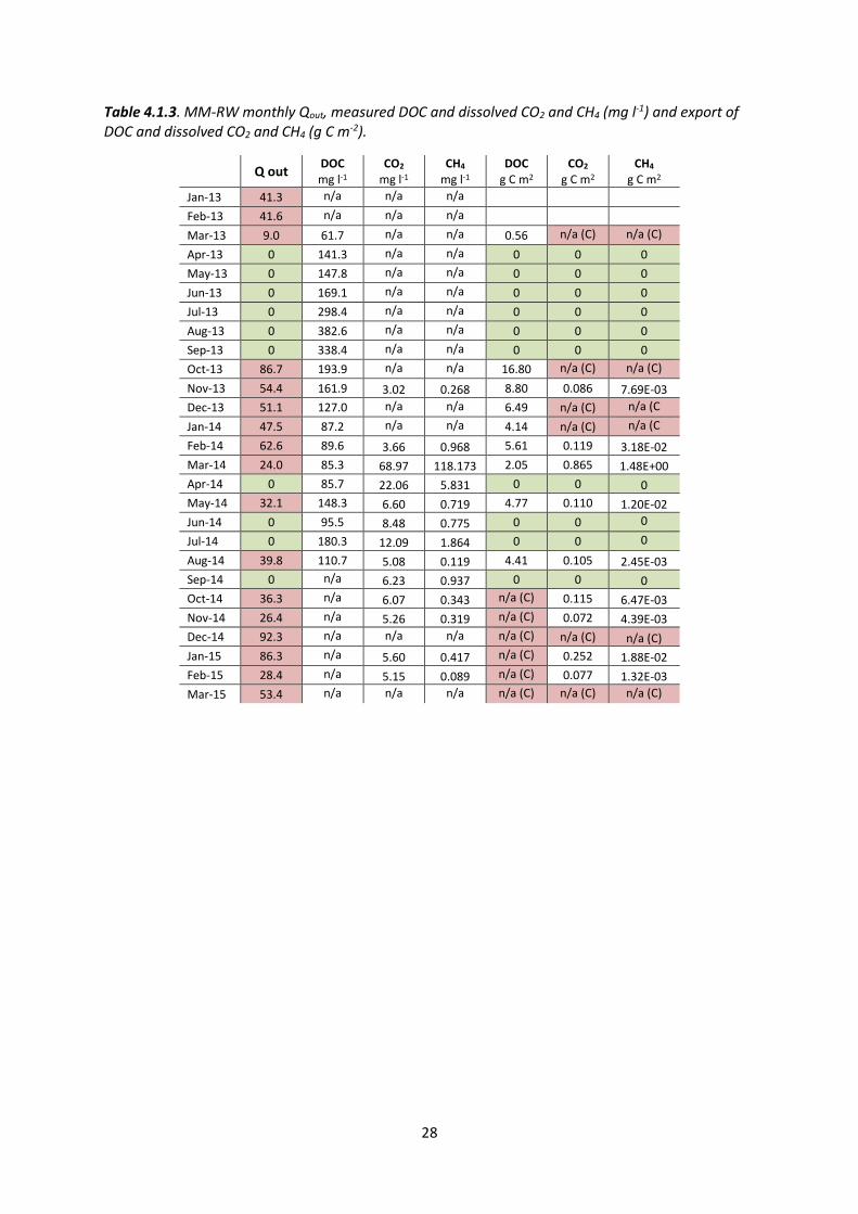
Table 4.1.3. MM-RW monthly Qout, measured DOC and dissolved CO2 and CH4 (mg l-1) and export of DOC and dissolved CO2 and CH4 (g C m-2).

Q out DOC mg l-1

CO2 mg l-1

CH4

mg l-1 DOC

g C m2 CO2

g C m2 CH4

g C m2

Jan-13 41.3 n/a n/a n/a

Feb-13 41.6 n/a n/a n/a

Mar-13 9.0 61.7 n/a n/a 0.56 n/a (C) n/a (C)

Apr-13 0 141.3 n/a n/a 0 0 0

May-13 0 147.8 n/a n/a 0 0 0

Jun-13 0 169.1 n/a n/a 0 0 0

Jul-13 0 298.4 n/a n/a 0 0 0

Aug-13 0 382.6 n/a n/a 0 0 0

Sep-13 0 338.4 n/a n/a 0 0 0

Oct-13 86.7 193.9 n/a n/a 16.80 n/a (C) n/a (C)

Nov-13 54.4 161.9 3.02 0.268 8.80 0.086 7.69E-03

Dec-13 51.1 127.0 n/a n/a 6.49 n/a (C) n/a (C

Jan-14 47.5 87.2 n/a n/a 4.14 n/a (C) n/a (C

Feb-14 62.6 89.6 3.66 0.968 5.61 0.119 3.18E-02

Mar-14 24.0 85.3 68.97 118.173 2.05 0.865 1.48E+00

Apr-14 0 85.7 22.06 5.831 0 0 0

May-14 32.1 148.3 6.60 0.719 4.77 0.110 1.20E-02

Jun-14 0 95.5 8.48 0.775 0 0 0

Jul-14 0 180.3 12.09 1.864 0 0 0

Aug-14 39.8 110.7 5.08 0.119 4.41 0.105 2.45E-03

Sep-14 0 n/a 6.23 0.937 0 0 0

Oct-14 36.3 n/a 6.07 0.343 n/a (C) 0.115 6.47E-03

Nov-14 26.4 n/a 5.26 0.319 n/a (C) 0.072 4.39E-03

Dec-14 92.3 n/a n/a n/a n/a (C) n/a (C) n/a (C)

Jan-15 86.3 n/a 5.60 0.417 n/a (C) 0.252 1.88E-02

Feb-15 28.4 n/a 5.15 0.089 n/a (C) 0.077 1.32E-03

Mar-15 53.4 n/a n/a n/a n/a (C) n/a (C) n/a (C)

29

Figure 4.1.2 Automated and manual water-table records at MM-RW from within the bunded area (panel A and B) and outside the bunded area (panel C and D)

30

Figure 4.1.3 Automated and manual water-table records at MM-RW from the different transects within the bunded area and outside the bunded area (bottom).

Figure 4.1.4 Water-table response to rainfall at MM-RW, the red line shows the 1:1 fit line.

31

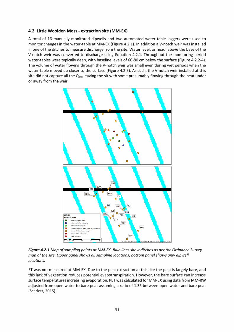
4.2. Little Woolden Moss - extraction site (MM-EX)

A total of 16 manually monitored dipwells and two automated water-table loggers were used to monitor changes in the water-table at MM-EX (Figure 4.2.1). In addition a V-notch weir was installed in one of the ditches to measure discharge from the site. Water level, or head, above the base of the V-notch weir was converted to discharge using Equation 4.2.1. Throughout the monitoring period water-tables were typically deep, with baseline levels of 60-80 cm below the surface (Figure 4.2.2-4). The volume of water flowing through the V-notch weir was small even during wet periods when the water-table moved up closer to the surface (Figure 4.2.5). As such, the V-notch weir installed at this site did not capture all the Qout leaving the sit with some presumably flowing through the peat under or away from the weir.

Figure 4.2.1 Map of sampling points at MM-EX. Blue lines show ditches as per the Ordnance Survey map of the site. Upper panel shows all sampling locations, bottom panel shows only dipwell locations.

ET was not measured at MM-EX. Due to the peat extraction at this site the peat is largely bare, and this lack of vegetation reduces potential evapotranspiration. However, the bare surface can increase surface temperatures increasing evaporation. PET was calculated for MM-EX using data from MM-RW adjusted from open water to bare peat assuming a ratio of 1.35 between open water and bare peat (Scarlett, 2015).

32

Discharge = 0.00112+(-0.00418*(h))+(0.01145*(h2))+(0.00159*(h3))) Equation 4.2.1

Where h is the head, or water level above the base of the V-notch

During summer months, ET typically exceeded rainfall preventing water export from the site (Table 4.2.1). For the remainder of the year the low baseline water-tables and the rapid response to rainfall indicated that where rainfall exceeds PET, water export occurs, although some of this was not captured by the V-notch weir.

Water quality samples were collected from the dipwells, and from the V-notch weir when it was flowing, during site visits.

33

Summary Results

Table 4.2.1. Monthly water budget for MM-EX. Qout is the total aquatic loss from the site. Pnet was gap filled for missing data. E derived from Thornthwaite (T) and Penman-Monteith (P-M) PET estimates.

Pnet

E

(T) Pnet –E

(T) E

(P-M) Pnet-E (P-M)

Qout

Dec-12 149.6 9.3 140.3 7.3 142.3 140.3

Jan-13 59.8 8.2 51.6 7.6 52.2 51.6

Feb-13 59.4 8.0 51.4 7.8 51.6 51.4

Mar-13 43.8 8.7 35.1 16.6 27.2 35.1

Apr-13 25.4 29.1 -3.7 27.6 -2.2 0

May-13 60.2 51.3 9.0 37.3 22.9 9.0

Jun-13 45.0 72.2 -27.2 44.6 0.4 0

Jul-13 60.6 93.8 -33.2 55.4 5.2 0

Aug-13 65.4 76.6 -11.2 47.0 18.4 0

Sep-13 63.0 50.8 12.2 34.9 28.1 12.2

Oct-13 139.0 38.9 100.1 24.3 114.7 100.1

Nov-13 89.0 13.9 75.1 14.5 74.5 75.1

Dec-13 70.0 14.1 56.0 7.3 62.7 56.0

Jan-14 66.0 11.7 54.3 7.6 58.4 54.3

Feb-14 80.4 14.2 66.2 7.8 72.6 66.2

Mar-14 58.8 22.8 36.0 16.6 42.2 36.0

Apr-14 49.8 40.0 9.8 27.6 22.2 9.8

May-14 106. 57.2 48.8 37.3 68.7 48.8

Jun-14 41.4 74.0 -32.6 44.6 -3.2 0

Jul-14 45.2 86.4 -41.2 55.4 -10.2 0

Aug-14 131.8 63.0 68.8 47.0 84.8 68.8

Sep-14 17.0 50.4 -33.4 34.9 -17.9 0

Oct-14 88.6 35.1 53.6 24.3 64.3 53.6

Nov-14 61.0 18.4 42.6 14.5 46.5 42.6

Dec-14 111.2 9.5 101.8 7.3 103.9 101.8

34

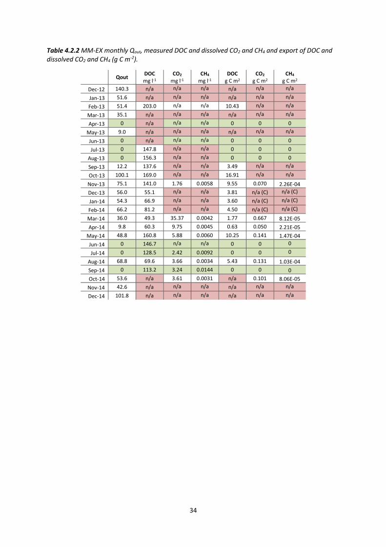
Table 4.2.2 MM-EX monthly Qout, measured DOC and dissolved CO2 and CH4 and export of DOC and dissolved CO2 and CH4 (g C m-2).

Qout DOC mg l-1

CO2 mg l-1

CH4

mg l-1 DOC

g C m2 CO2

g C m2 CH4

g C m2

Dec-12 140.3 n/a n/a n/a n/a n/a n/a

Jan-13 51.6 n/a n/a n/a n/a n/a n/a

Feb-13 51.4 203.0 n/a n/a 10.43 n/a n/a

Mar-13 35.1 n/a n/a n/a n/a n/a n/a

Apr-13 0 n/a n/a n/a 0 0 0

May-13 9.0 n/a n/a n/a n/a n/a n/a

Jun-13 0 n/a n/a n/a 0 0 0

Jul-13 0 147.8 n/a n/a 0 0 0

Aug-13 0 156.3 n/a n/a 0 0 0

Sep-13 12.2 137.6 n/a n/a 3.49 n/a n/a

Oct-13 100.1 169.0 n/a n/a 16.91 n/a n/a

Nov-13 75.1 141.0 1.76 0.0058 9.55 0.070 2.26E-04

Dec-13 56.0 55.1 n/a n/a 3.81 n/a (C) n/a (C)

Jan-14 54.3 66.9 n/a n/a 3.60 n/a (C) n/a (C)

Feb-14 66.2 81.2 n/a n/a 4.50 n/a (C) n/a (C)

Mar-14 36.0 49.3 35.37 0.0042 1.77 0.667 8.12E-05

Apr-14 9.8 60.3 9.75 0.0045 0.63 0.050 2.21E-05

May-14 48.8 160.8 5.88 0.0060 10.25 0.141 1.47E-04

Jun-14 0 146.7 n/a n/a 0 0 0

Jul-14 0 128.5 2.42 0.0092 0 0 0

Aug-14 68.8 69.6 3.66 0.0034 5.43 0.131 1.03E-04

Sep-14 0 113.2 3.24 0.0144 0 0 0

Oct-14 53.6 n/a 3.61 0.0031 n/a 0.101 8.06E-05

Nov-14 42.6 n/a n/a n/a n/a n/a n/a

Dec-14 101.8 n/a n/a n/a n/a n/a n/a

35

Figure 4.2.2 Automated (top panel) and manual (middle panel) water-table records from MM-EX with (bottom panel) discharge (red) and water depth above the V-notch (black).

36

Figure 4.2.3 Automated and manual water-table records from the MM-EX south-north transects

37

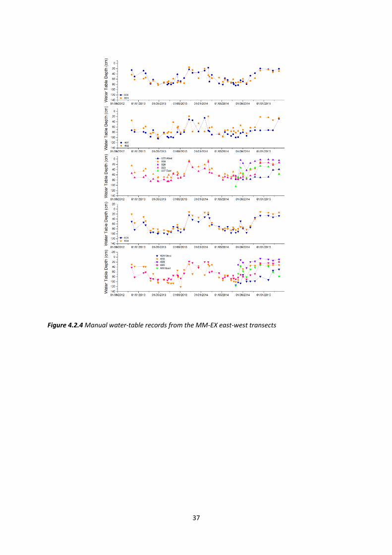
Figure 4.2.4 Manual water-table records from the MM-EX east-west transects

38

Figure 4.2.5 Automated water-table records (red and black) and water depth at the V-notch weir (blue) at MM-EX for the whole record (top panel), winter 2013 (middle panel) and winter 2014 (bottom panel).

39

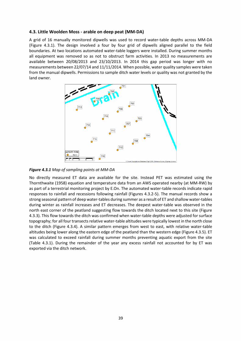
4.3. Little Woolden Moss - arable on deep peat (MM-DA)

A grid of 16 manually monitored dipwells was used to record water-table depths across MM-DA (Figure 4.3.1). The design involved a four by four grid of dipwells aligned parallel to the field boundaries. At two locations automated water-table loggers were installed. During summer months all equipment was removed so as not to obstruct farm activities. In 2013 no measurements are available between 20/08/2013 and 23/10/2013. In 2014 this gap period was longer with no measurements between 22/07/14 and 11/11/2014. When possible, water quality samples were taken from the manual dipwells. Permissions to sample ditch water levels or quality was not granted by the land owner.

Figure 4.3.1 Map of sampling points at MM-DA

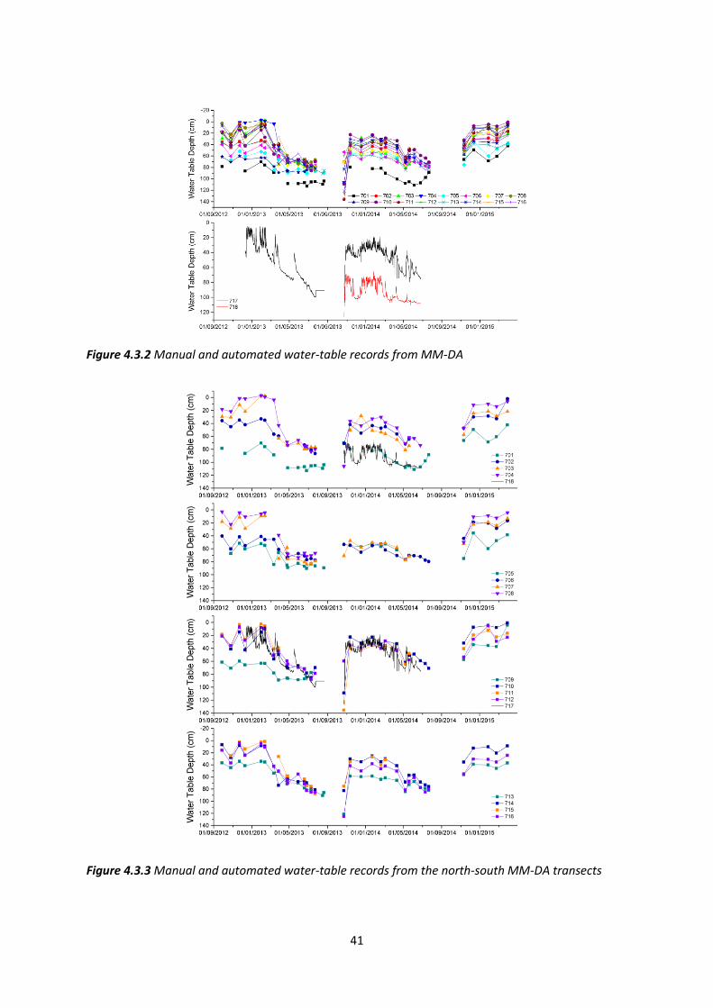
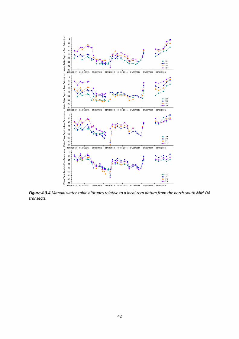
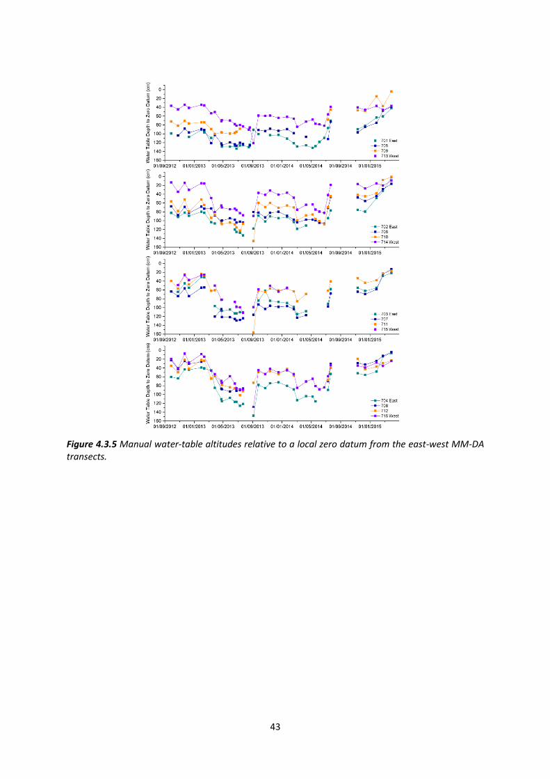
No directly measured ET data are available for the site. Instead PET was estimated using the Thornthwaite (1958) equation and temperature data from an AWS operated nearby (at MM-RW) by as part of a terrestrial monitoring project by E.On. The automated water-table records indicate rapid responses to rainfall and recessions following rainfall (Figures 4.3.2-5). The manual records show a strong seasonal pattern of deep water-tables during summer as a result of ET and shallow water-tables during winter as rainfall increases and ET decreases. The deepest water-table was observed in the north east corner of the peatland suggesting flow towards the ditch located next to this site (Figure 4.3.3). This flow towards the ditch was confirmed when water-table depths were adjusted for surface topography; for all four transects relative water-table altitudes were typically lowest in the north close to the ditch (Figure 4.3.4). A similar pattern emerges from west to east, with relative water-table altitudes being lower along the eastern edge of the peatland than the western edge (Figure 4.3.5). ET was calculated to exceed rainfall during summer months preventing aquatic export from the site (Table 4.3.1). During the remainder of the year any excess rainfall not accounted for by ET was exported via the ditch network.

40

Table 4.3.1 Monthly water budget for MM-DA. Qout is the total aquatic loss from the site

Pnet E Pnet-E Q out

Jun-13 45.0 86.84 -41.84 0

Jul-13 60.6 88.09 -27.49 0

Aug-13 65.4 69.25 -3.85 0

Sep-13 63.0 48.46 14.54 14.5

Oct-13 139.0 27.08 111.92 111.9

Nov-13 89.0 15.67 73.33 73.3

Dec-13 70.0 10.19 59.81 59.8

Jan-14 66.0 13.63 52.37 52.4

Feb-14 80.4 16.49 63.91 63.9

Mar-14 58.8 39.14 19.66 19.7

Apr-14 49.8 59.98 -10.18 0

May-14 106.0 83.80 22.20 22.2

Jun-14 41.4 86.84 -45.44 0

Jul-14 45.2 88.09 -42.89 0

Aug-14 131.8 69.25 62.55 62.6

Sep-14 17.0 48.46 -31.46 0

Oct-14 88.6 27.08 61.52 61.5

Nov-14 61.0 15.67 45.33 45.3

Dec-14 111.2 10.19 101.01 101.0

Table 4.3.2 MM-DA monthly Qout, measured DOC (mg l-1) and DOC export (g C m-2)

Q out DOC

mg l-1 DOC

g C m2

Jun-13 0 209.3 0

Jul-13 0 278.7 0

Aug-13 0 271.9 0

Sep-13 14.5 n/a n/a

Oct-13 111.9 n/a n/a

Nov-13 73.3 130.4 9.56

Dec-13 59.8 46.0 2.75

Jan-14 52.4 39.2 2.05

Feb-14 63.9 48.3 3.09

Mar-14 19.7 70.4 1.38

Apr-14 0 102.8 0

May-14 22.2 243.3 5.40

Jun-14 0 151.9 0

Jul-14 0 n/a 0

Aug-14 62.6 n/a n/a

Sep-14 0 n/a 0

Oct-14 61.5 n/a n/a

Nov-14 45.3 n/a n/a

Dec-14 101.0 n/a n/a

41

Figure 4.3.2 Manual and automated water-table records from MM-DA

Figure 4.3.3 Manual and automated water-table records from the north-south MM-DA transects

42

Figure 4.3.4 Manual water-table altitudes relative to a local zero datum from the north-south MM-DA transects.

43

Figure 4.3.5 Manual water-table altitudes relative to a local zero datum from the east-west MM-DA transects.

44

5. Anglesey Fens

5.1. Cors Erddreiniog – Low nutrient fen (AF-LN)

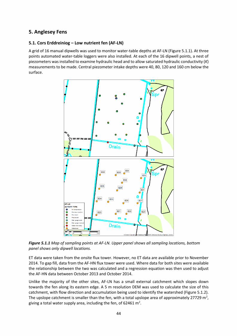
A grid of 16 manual dipwells was used to monitor water-table depths at AF-LN (Figure 5.1.1). At three points automated water-table loggers were also installed. At each of the 16 dipwell points, a nest of piezometers was installed to examine hydraulic head and to allow saturated hydraulic conductivity (K) measurements to be made. Central piezometer intake depths were 40, 80, 120 and 160 cm below the surface.

Figure 5.1.1 Map of sampling points at AF-LN. Upper panel shows all sampling locations, bottom panel shows only dipwell locations.

ET data were taken from the onsite flux tower. However, no ET data are available prior to November 2014. To gap fill, data from the AF-HN flux tower were used. Where data for both sites were available the relationship between the two was calculated and a regression equation was then used to adjust the AF-HN data between October 2013 and October 2014.

Unlike the majority of the other sites, AF-LN has a small external catchment which slopes down towards the fen along its eastern edge. A 5 m resolution DEM was used to calculate the size of this catchment, with flow direction and accumulation being used to identify the watershed (Figure 5.1.2). The upslope catchment is smaller than the fen, with a total upslope area of approximately 27729 m2, giving a total water supply area, including the fen, of 62461 m2.

45

Figure 5.1.2 Map showing flow accumulation across AF-LN and the watershed of the catchment upslope of AF-LN, both of which were calculated using the DEM of the site.

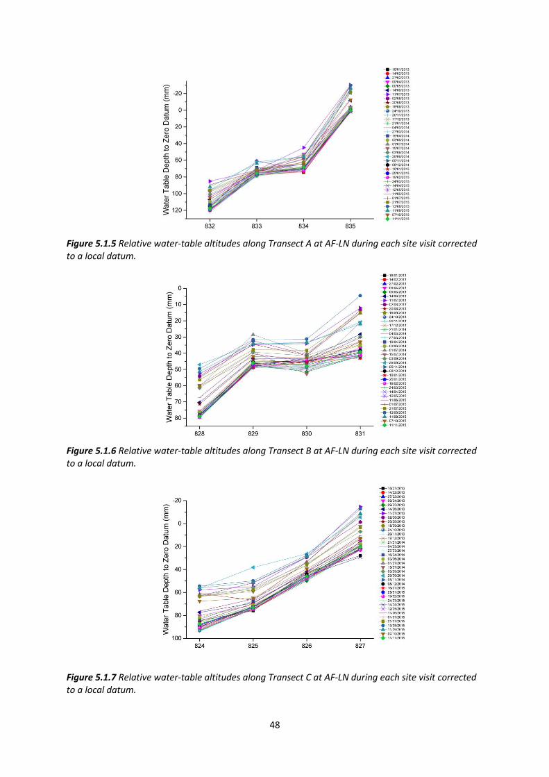
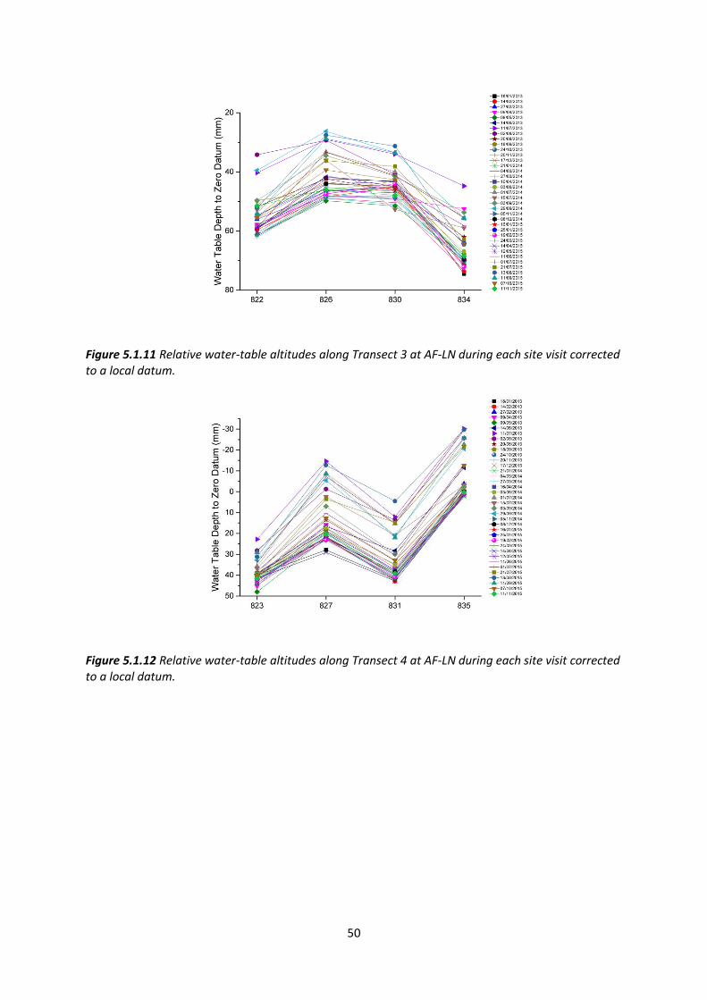
The grid of dipwells and piezometers were grouped by transect to identify differences across the site, with transects 1 to 4 running north-south and transects A to D running east-west (Figure 5.1.3). Water-tables were deepest at the east and west of the site, suggesting a domed water-table. However, when surface topography was examined, a steep hydraulic gradient was observed, with lowest relative water-table altitudes in the western part of the fen (Figures 5.1.5-8). The north-south transects indicated that the water-table across the site was more complex than a simple east-west gradient. Along transect 1 at the western edge of the fen relative water-table altitudes were lowest in the north and highest in the south as water flows towards the lake (Figure 5.1.9). The same was also partly true for transect 2, with some flow towards the lake in the north of the site; however, in this case the water-table was at a lower altitude at sample point 825 than at sample point 829 indicating that not all flow was south to north (Figure 5.1.10). Transect 3 suggests a domed structure to the relative water-table heights, with shallowest water-tables in the middle of the fen (Figure 5.1.11). For transect 4, highest water-table altitudes were in the north and lowest in the south (Figure 5.1.12), but, as with transect 2, not all flow was north to south.

© Crown Copyright and Database Right 2016. Ordnance Survey (Digimap Licence)

46

1 2 3 4

A

832 833 834 835

B

828 829 830 831

C

824 825 826 827

D

820 821 822 823

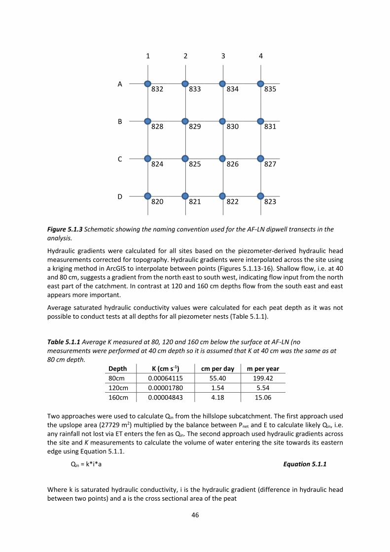
Figure 5.1.3 Schematic showing the naming convention used for the AF-LN dipwell transects in the analysis.

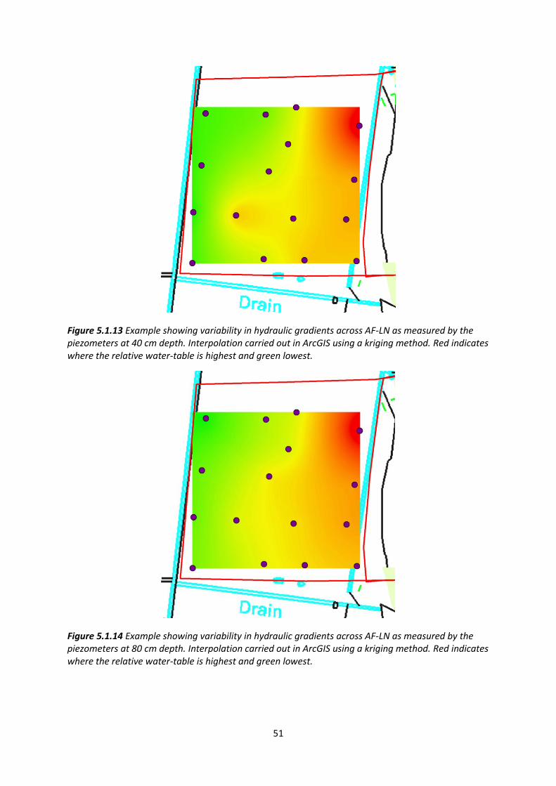
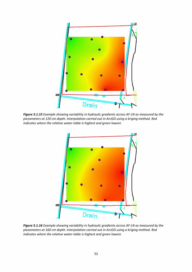
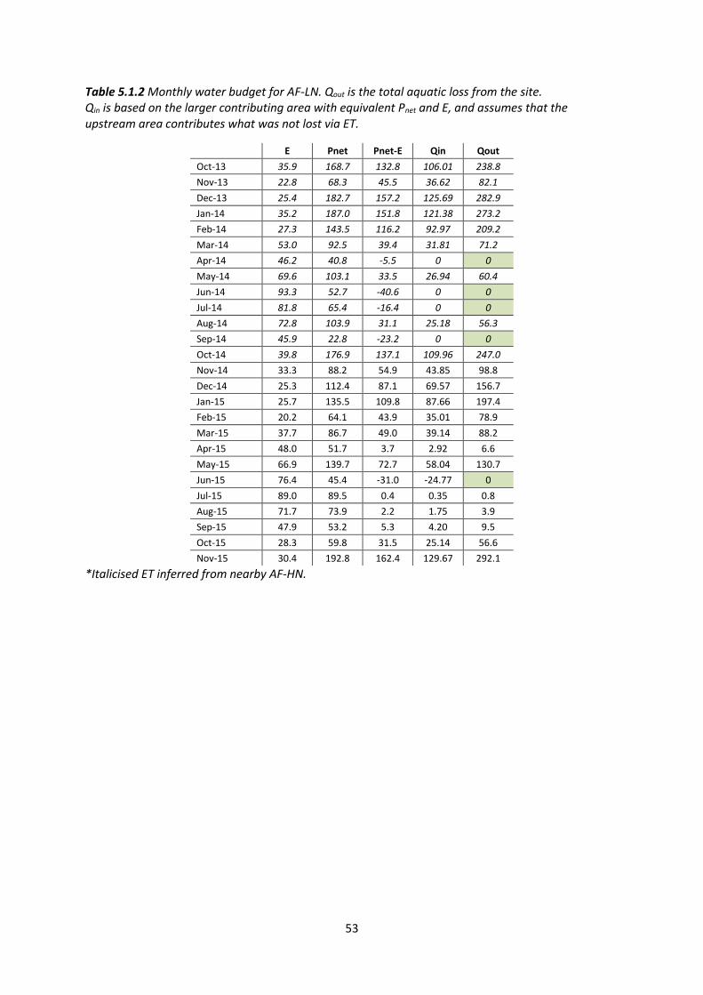
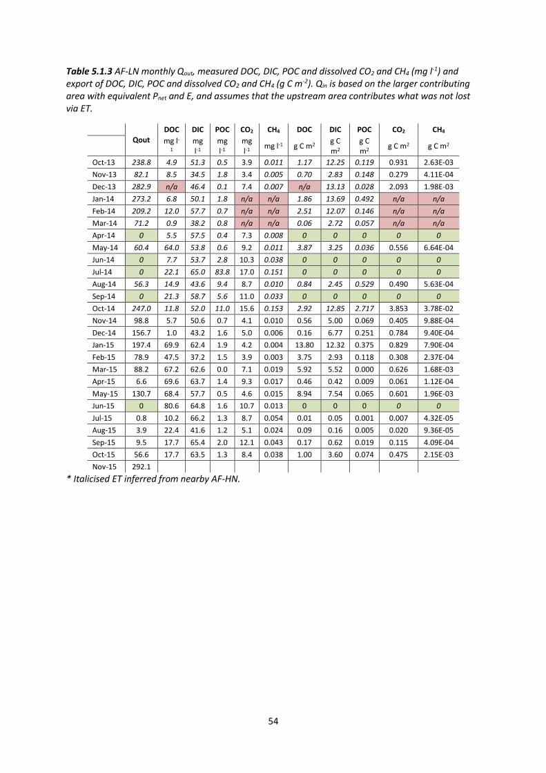
Hydraulic gradients were calculated for all sites based on the piezometer-derived hydraulic head measurements corrected for topography. Hydraulic gradients were interpolated across the site using a kriging method in ArcGIS to interpolate between points (Figures 5.1.13-16). Shallow flow, i.e. at 40 and 80 cm, suggests a gradient from the north east to south west, indicating flow input from the north east part of the catchment. In contrast at 120 and 160 cm depths flow from the south east and east appears more important.

Average saturated hydraulic conductivity values were calculated for each peat depth as it was not possible to conduct tests at all depths for all piezometer nests (Table 5.1.1).

Table 5.1.1 Average K measured at 80, 120 and 160 cm below the surface at AF-LN (no measurements were performed at 40 cm depth so it is assumed that K at 40 cm was the same as at 80 cm depth.

Depth K (cm s-1) cm per day m per year

80cm 0.00064115 55.40 199.42

120cm 0.00001780 1.54 5.54

160cm 0.00004843 4.18 15.06

Two approaches were used to calculate Qin from the hillslope subcatchment. The first approach used the upslope area (27729 m2) multiplied by the balance between Pnet and E to calculate likely Qin, i.e. any rainfall not lost via ET enters the fen as Qin. The second approach used hydraulic gradients across the site and K measurements to calculate the volume of water entering the site towards its eastern edge using Equation 5.1.1.

Qin = k*i*a Equation 5.1.1

Where k is saturated hydraulic conductivity, i is the hydraulic gradient (difference in hydraulic head between two points) and a is the cross sectional area of the peat

47

Qout was also calculated for the western side of the site using Equation 5.1.1. However, Qout was calculated to be lower than Qin suggesting not all flow moves in a simple east to west direction, with flow also lost to the lake in the north.

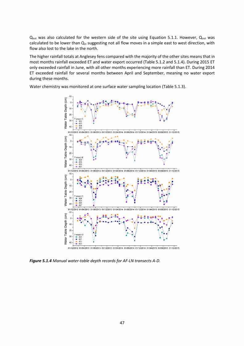
The higher rainfall totals at Anglesey fens compared with the majority of the other sites means that in most months rainfall exceeded ET and water export occurred (Table 5.1.2 and 5.1.4). During 2015 ET only exceeded rainfall in June, with all other months experiencing more rainfall than ET. During 2014 ET exceeded rainfall for several months between April and September, meaning no water export during these months.

Water chemistry was monitored at one surface water sampling location (Table 5.1.3).

Figure 5.1.4 Manual water-table depth records for AF-LN transects A-D.

48

Figure 5.1.5 Relative water-table altitudes along Transect A at AF-LN during each site visit corrected to a local datum.

Figure 5.1.6 Relative water-table altitudes along Transect B at AF-LN during each site visit corrected to a local datum.

Figure 5.1.7 Relative water-table altitudes along Transect C at AF-LN during each site visit corrected to a local datum.

49

Figure 5.1.8 Relative water-table altitudes along Transect D at AF-LN during each site visit corrected to a local datum.

Figure 5.1.9 Relative water-table altitudes along Transect 1 at AF-LN during each site visit corrected to a local datum.


50



51

Figure 5.1.13 Example showing variability in hydraulic gradients across AF-LN as measured by the piezometers at 40 cm depth. Interpolation carried out in ArcGIS using a kriging method. Red indicates where the relative water-table is highest and green lowest.


52



53

Table 5.1.2 Monthly water budget for AF-LN. Qout is the total aquatic loss from the site. Qin is based on the larger contributing area with equivalent Pnet and E, and assumes that the upstream area contributes what was not lost via ET.

E Pnet Pnet-E Qin Qout

Oct-13 35.9 168.7 132.8 106.01 238.8

Nov-13 22.8 68.3 45.5 36.62 82.1

Dec-13 25.4 182.7 157.2 125.69 282.9

Jan-14 35.2 187.0 151.8 121.38 273.2

Feb-14 27.3 143.5 116.2 92.97 209.2

Mar-14 53.0 92.5 39.4 31.81 71.2

Apr-14 46.2 40.8 -5.5 0 0

May-14 69.6 103.1 33.5 26.94 60.4

Jun-14 93.3 52.7 -40.6 0 0

Jul-14 81.8 65.4 -16.4 0 0

Aug-14 72.8 103.9 31.1 25.18 56.3

Sep-14 45.9 22.8 -23.2 0 0

Oct-14 39.8 176.9 137.1 109.96 247.0

Nov-14 33.3 88.2 54.9 43.85 98.8

Dec-14 25.3 112.4 87.1 69.57 156.7

Jan-15 25.7 135.5 109.8 87.66 197.4

Feb-15 20.2 64.1 43.9 35.01 78.9

Mar-15 37.7 86.7 49.0 39.14 88.2

Apr-15 48.0 51.7 3.7 2.92 6.6

May-15 66.9 139.7 72.7 58.04 130.7

Jun-15 76.4 45.4 -31.0 -24.77 0

Jul-15 89.0 89.5 0.4 0.35 0.8

Aug-15 71.7 73.9 2.2 1.75 3.9

Sep-15 47.9 53.2 5.3 4.20 9.5

Oct-15 28.3 59.8 31.5 25.14 56.6

Nov-15 30.4 192.8 162.4 129.67 292.1

*Italicised ET inferred from nearby AF-HN.

54

Table 5.1.3 AF-LN monthly Qout, measured DOC, DIC, POC and dissolved CO2 and CH4 (mg l-1) and export of DOC, DIC, POC and dissolved CO2 and CH4 (g C m-2). Qin is based on the larger contributing area with equivalent Pnet and E, and assumes that the upstream area contributes what was not lost via ET.

Qout


mg l-

1 mg l-1

mg l-1

mg l-1

mg l-1 g C m2 g C m2

g C m2

g C m2 g C m2

Oct-13 238.8 4.9 51.3 0.5 3.9 0.011 1.17 12.25 0.119 0.931 2.63E-03

Nov-13 82.1 8.5 34.5 1.8 3.4 0.005 0.70 2.83 0.148 0.279 4.11E-04

Dec-13 282.9 n/a 46.4 0.1 7.4 0.007 n/a 13.13 0.028 2.093 1.98E-03

Jan-14 273.2 6.8 50.1 1.8 n/a n/a 1.86 13.69 0.492 n/a n/a

Feb-14 209.2 12.0 57.7 0.7 n/a n/a 2.51 12.07 0.146 n/a n/a

Mar-14 71.2 0.9 38.2 0.8 n/a n/a 0.06 2.72 0.057 n/a n/a

Apr-14 0 5.5 57.5 0.4 7.3 0.008 0 0 0 0 0

May-14 60.4 64.0 53.8 0.6 9.2 0.011 3.87 3.25 0.036 0.556 6.64E-04

Jun-14 0 7.7 53.7 2.8 10.3 0.038 0 0 0 0 0

Jul-14 0 22.1 65.0 83.8 17.0 0.151 0 0 0 0 0

Aug-14 56.3 14.9 43.6 9.4 8.7 0.010 0.84 2.45 0.529 0.490 5.63E-04

Sep-14 0 21.3 58.7 5.6 11.0 0.033 0 0 0 0 0

Oct-14 247.0 11.8 52.0 11.0 15.6 0.153 2.92 12.85 2.717 3.853 3.78E-02

Nov-14 98.8 5.7 50.6 0.7 4.1 0.010 0.56 5.00 0.069 0.405 9.88E-04

Dec-14 156.7 1.0 43.2 1.6 5.0 0.006 0.16 6.77 0.251 0.784 9.40E-04

Jan-15 197.4 69.9 62.4 1.9 4.2 0.004 13.80 12.32 0.375 0.829 7.90E-04

Feb-15 78.9 47.5 37.2 1.5 3.9 0.003 3.75 2.93 0.118 0.308 2.37E-04

Mar-15 88.2 67.2 62.6 0.0 7.1 0.019 5.92 5.52 0.000 0.626 1.68E-03

Apr-15 6.6 69.6 63.7 1.4 9.3 0.017 0.46 0.42 0.009 0.061 1.12E-04

May-15 130.7 68.4 57.7 0.5 4.6 0.015 8.94 7.54 0.065 0.601 1.96E-03

Jun-15 0 80.6 64.8 1.6 10.7 0.013 0 0 0 0 0

Jul-15 0.8 10.2 66.2 1.3 8.7 0.054 0.01 0.05 0.001 0.007 4.32E-05

Aug-15 3.9 22.4 41.6 1.2 5.1 0.024 0.09 0.16 0.005 0.020 9.36E-05

Sep-15 9.5 17.7 65.4 2.0 12.1 0.043 0.17 0.62 0.019 0.115 4.09E-04

Oct-15 56.6 17.7 63.5 1.3 8.4 0.038 1.00 3.60 0.074 0.475 2.15E-03

Nov-15 292.1

* Italicised ET inferred from nearby AF-HN.

55

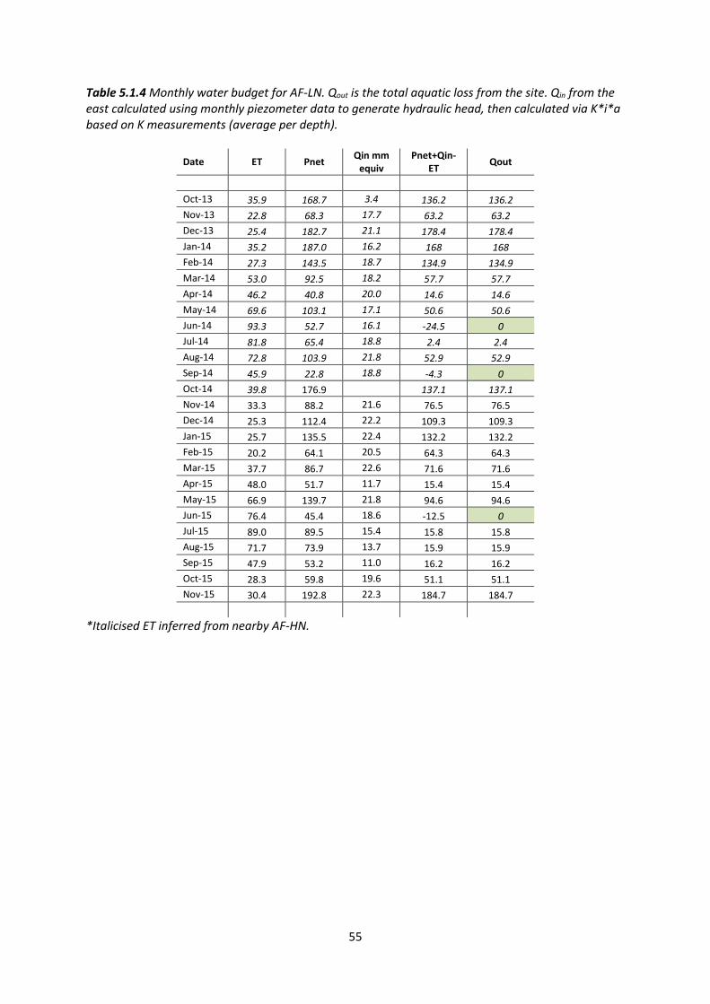
Table 5.1.4 Monthly water budget for AF-LN. Qout is the total aquatic loss from the site. Qin from the east calculated using monthly piezometer data to generate hydraulic head, then calculated via K*i*a based on K measurements (average per depth).

Date ET Pnet Qin mm

equiv Pnet+Qin-

ET Qout

Oct-13 35.9 168.7 3.4 136.2 136.2

Nov-13 22.8 68.3 17.7 63.2 63.2

Dec-13 25.4 182.7 21.1 178.4 178.4

Jan-14 35.2 187.0 16.2 168 168

Feb-14 27.3 143.5 18.7 134.9 134.9

Mar-14 53.0 92.5 18.2 57.7 57.7

Apr-14 46.2 40.8 20.0 14.6 14.6

May-14 69.6 103.1 17.1 50.6 50.6

Jun-14 93.3 52.7 16.1 -24.5 0

Jul-14 81.8 65.4 18.8 2.4 2.4

Aug-14 72.8 103.9 21.8 52.9 52.9

Sep-14 45.9 22.8 18.8 -4.3 0

Oct-14 39.8 176.9 137.1 137.1

Nov-14 33.3 88.2 21.6 76.5 76.5

Dec-14 25.3 112.4 22.2 109.3 109.3

Jan-15 25.7 135.5 22.4 132.2 132.2

Feb-15 20.2 64.1 20.5 64.3 64.3

Mar-15 37.7 86.7 22.6 71.6 71.6

Apr-15 48.0 51.7 11.7 15.4 15.4

May-15 66.9 139.7 21.8 94.6 94.6

Jun-15 76.4 45.4 18.6 -12.5 0

Jul-15 89.0 89.5 15.4 15.8 15.8

Aug-15 71.7 73.9 13.7 15.9 15.9

Sep-15 47.9 53.2 11.0 16.2 16.2

Oct-15 28.3 59.8 19.6 51.1 51.1

Nov-15 30.4 192.8 22.3 184.7 184.7


56

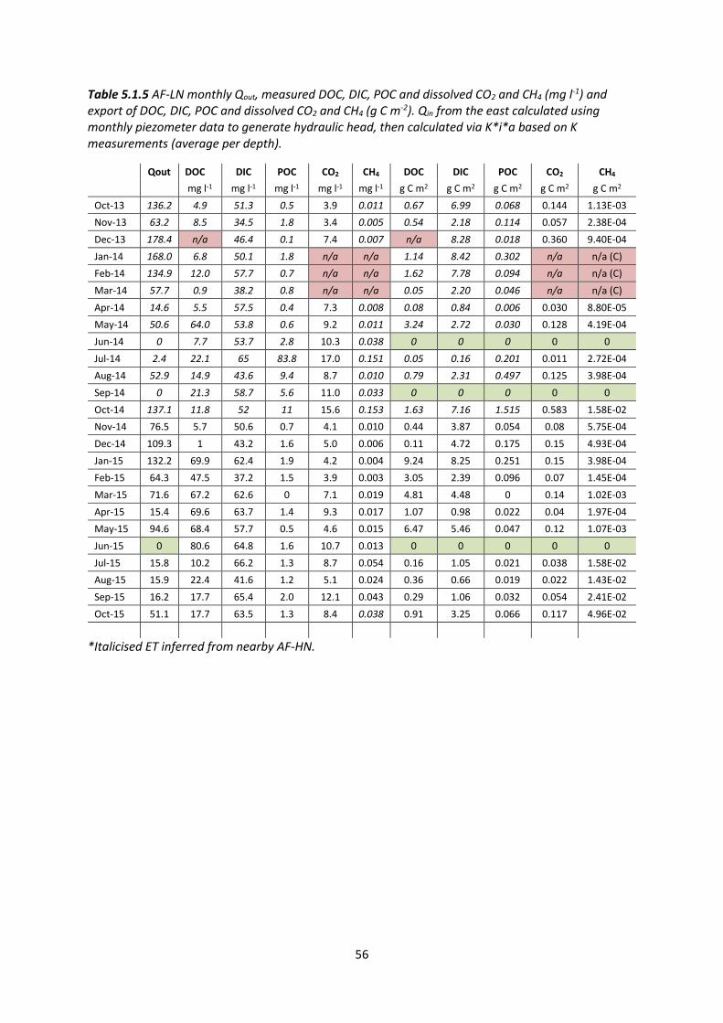
Table 5.1.5 AF-LN monthly Qout, measured DOC, DIC, POC and dissolved CO2 and CH4 (mg l-1) and export of DOC, DIC, POC and dissolved CO2 and CH4 (g C m-2). Qin from the east calculated using monthly piezometer data to generate hydraulic head, then calculated via K*i*a based on K measurements (average per depth).

Qout DOC DIC POC CO2 CH4 DOC DIC POC CO2 CH4


Oct-13 136.2 4.9 51.3 0.5 3.9 0.011 0.67 6.99 0.068 0.144 1.13E-03

Nov-13 63.2 8.5 34.5 1.8 3.4 0.005 0.54 2.18 0.114 0.057 2.38E-04

Dec-13 178.4 n/a 46.4 0.1 7.4 0.007 n/a 8.28 0.018 0.360 9.40E-04

Jan-14 168.0 6.8 50.1 1.8 n/a n/a 1.14 8.42 0.302 n/a n/a (C)

Feb-14 134.9 12.0 57.7 0.7 n/a n/a 1.62 7.78 0.094 n/a n/a (C)

Mar-14 57.7 0.9 38.2 0.8 n/a n/a 0.05 2.20 0.046 n/a n/a (C)

Apr-14 14.6 5.5 57.5 0.4 7.3 0.008 0.08 0.84 0.006 0.030 8.80E-05

May-14 50.6 64.0 53.8 0.6 9.2 0.011 3.24 2.72 0.030 0.128 4.19E-04

Jun-14 0 7.7 53.7 2.8 10.3 0.038 0 0 0 0 0

Jul-14 2.4 22.1 65 83.8 17.0 0.151 0.05 0.16 0.201 0.011 2.72E-04

Aug-14 52.9 14.9 43.6 9.4 8.7 0.010 0.79 2.31 0.497 0.125 3.98E-04

Sep-14 0 21.3 58.7 5.6 11.0 0.033 0 0 0 0 0

Oct-14 137.1 11.8 52 11 15.6 0.153 1.63 7.16 1.515 0.583 1.58E-02

Nov-14 76.5 5.7 50.6 0.7 4.1 0.010 0.44 3.87 0.054 0.08 5.75E-04

Dec-14 109.3 1 43.2 1.6 5.0 0.006 0.11 4.72 0.175 0.15 4.93E-04

Jan-15 132.2 69.9 62.4 1.9 4.2 0.004 9.24 8.25 0.251 0.15 3.98E-04

Feb-15 64.3 47.5 37.2 1.5 3.9 0.003 3.05 2.39 0.096 0.07 1.45E-04

Mar-15 71.6 67.2 62.6 0 7.1 0.019 4.81 4.48 0 0.14 1.02E-03

Apr-15 15.4 69.6 63.7 1.4 9.3 0.017 1.07 0.98 0.022 0.04 1.97E-04

May-15 94.6 68.4 57.7 0.5 4.6 0.015 6.47 5.46 0.047 0.12 1.07E-03

Jun-15 0 80.6 64.8 1.6 10.7 0.013 0 0 0 0 0

Jul-15 15.8 10.2 66.2 1.3 8.7 0.054 0.16 1.05 0.021 0.038 1.58E-02

Aug-15 15.9 22.4 41.6 1.2 5.1 0.024 0.36 0.66 0.019 0.022 1.43E-02

Sep-15 16.2 17.7 65.4 2.0 12.1 0.043 0.29 1.06 0.032 0.054 2.41E-02

Oct-15 51.1 17.7 63.5 1.3 8.4 0.038 0.91 3.25 0.066 0.117 4.96E-02


57

5.2. Cors Erddreiniog – High nutrient fen (AF-HN)

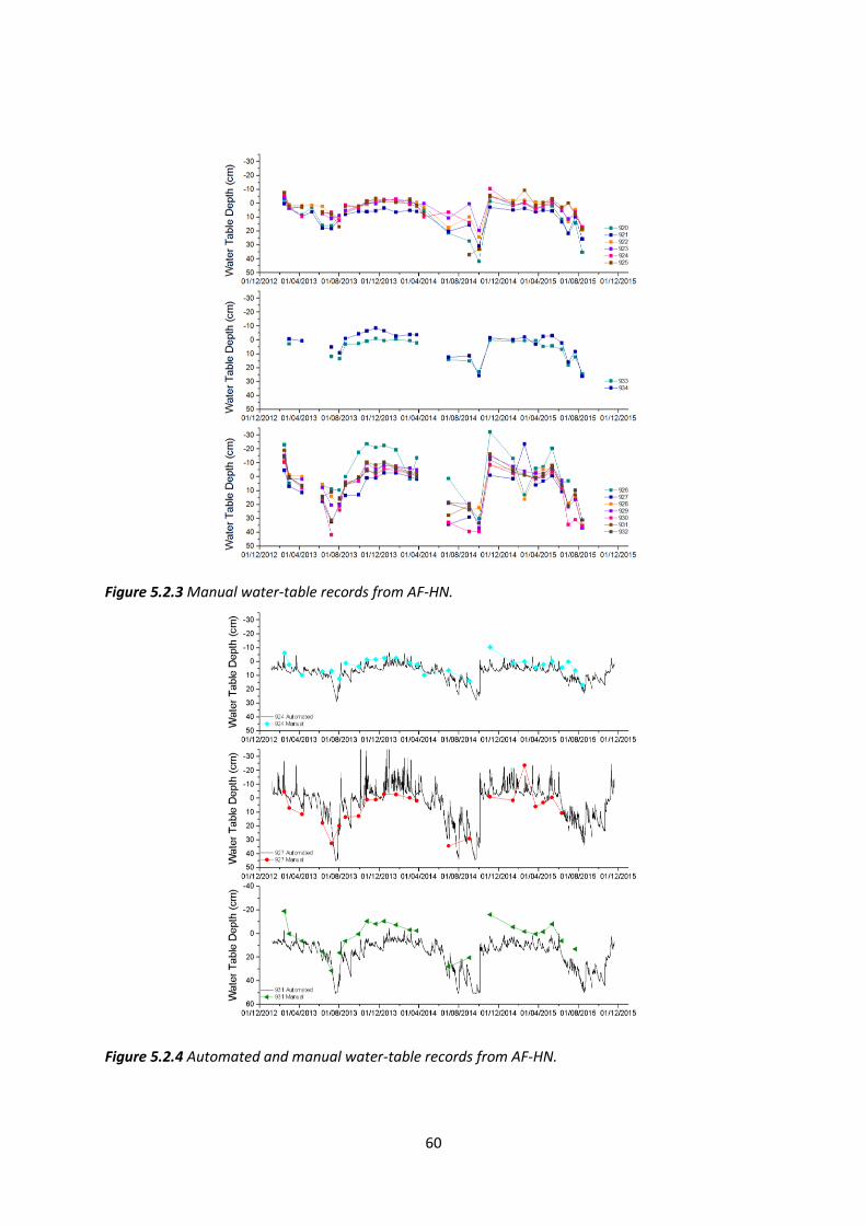
At AF-HN fen, 15 manually recording dipwells and three with automated water-table loggers were used to monitor the water-table (Figure 5.2.1). A set of seven manual dipwells were located along the

southern edge of the fen, with the remainder in the north.

Figure 5.2.1 Map of sampling points at AF-HN. Upper panel shows all sampling locations, bottom panel shows only dipwell locations.

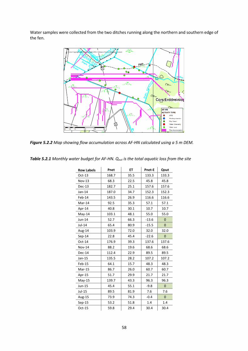
ET data were taken from the onsite flux tower while rainfall data were taken from the onsite AWS. As with AF-LN, topographic analysis was undertaken to identify whether the site had a contributing subcatchment. However, flow accumulation across the site indicated that the site was unlikely to have a significant catchment outside of the drains so it was assumed that there was no Qin (Figure 5.2.2). When changes in surface topography are taken into account there was a general east to west gradient in relative water-table altitudes along the southern edge of the fen, with water-table altitudes being highest in the east and lowest in the west. Along the northern edge of the fen the deepest water-tables occur in the west when adjusted for altitude. Water is likely to move across site from east to west, draining into surrounding ditches. The high rainfall totals at the site result in rainfall exceeding ET for most months of the year, except during summer and early autumn (Table 5.2.1). When rainfall exceeds ET, water export occurs from the fen. During those months where ET exceeds rainfall no water export occurs.

58

Water samples were collected from the two ditches running along the northern and southern edge of the fen.

Figure 5.2.2 Map showing flow accumulation across AF-HN calculated using a 5 m DEM.

Table 5.2.1 Monthly water budget for AF-HN. Qout is the total aquatic loss from the site

Row Labels Pnet ET Pnet-E Qout

Oct-13 168.7 35.5 133.3 133.3

Nov-13 68.3 22.5 45.8 45.8

Dec-13 182.7 25.1 157.6 157.6

Jan-14 187.0 34.7 152.3 152.3

Feb-14 143.5 26.9 116.6 116.6

Mar-14 92.5 35.3 57.1 57.1

Apr-14 40.8 30.1 10.7 10.7

May-14 103.1 48.1 55.0 55.0

Jun-14 52.7 66.3 -13.6 0

Jul-14 65.4 80.9 -15.5 0

Aug-14 103.9 72.0 32.0 32.0

Sep-14 22.8 45.4 -22.6 0

Oct-14 176.9 39.3 137.6 137.6

Nov-14 88.2 19.6 68.6 68.6

Dec-14 112.4 22.9 89.5 89.5

Jan-15 135.5 28.2 107.2 107.2

Feb-15 64.1 15.7 48.3 48.3

Mar-15 86.7 26.0 60.7 60.7

Apr-15 51.7 29.9 21.7 21.7

May-15 139.7 43.3 96.3 96.3

Jun-15 45.4 55.1 -9.8 0

Jul-15 89.5 81.9 7.6 7.6

Aug-15 73.9 74.3 -0.4 0

Sep-15 53.2 51.8 1.4 1.4

Oct-15 59.8 29.4 30.4 30.4

© Crown Copyright and Database Right 2016. Ordnance Survey (Digimap Licence)

59

Table 5.2.2 AF-HN monthly Qout, measured DOC, DIC, POC and dissolved CO2 and CH4 (mg l-1) and export of DOC, DIC, POC and dissolved CO2 and CH4 (g C m-2).

Qout DOC DIC POC CO2 CH4 DOC DIC POC CO2 CH4


Oct-13 133.3 48.2 31.0 1.9 6.3 0.007 6.43 4.13 0.253 0.232 6.85E-04

Nov-13 45.8 41.2 18.5 8.4 3.4 0.005 1.89 0.85 0.385 0.044 1.59E-04

Dec-13 157.6 44.5 16.8 17.4 7.3 0.005 7.01 2.65 2.742 0.313 5.65E-04

Jan-14 152.3 42.0 18.1 22.6 n/a (C) n/a (C) 6.40 2.76 3.442 n/a (C) n/a (C)

Feb-14 116.6 34.3 17.9 1.7 5.6 0.036 4.00 2.09 0.198 0.177 3.17E-03

Mar-14 57.1 34.2 23.9 32.2 n/a (C) n/a (C) 1.95 1.36 1.839 n/a (C) n/a (C)

Apr-14 10.7 48.2 14.2 33.8 16.0 0.012 0.52 0.15 0.362 0.046 9.70E-05

May-14 55.0 76.4 32.4 10.4 11.5 0.041 4.20 1.78 0.572 0.172 1.69E-03

Jun-14 0 59.4 41.4 11.1 13.3 0.227 0 0 0 0 0

Jul-14 0 n/a (C) n/a (C) n/a (C) n/a (C) n/a (C) 0 0 0 0 0

Aug-14 32.0 n/a (C) n/a (C) n/a (C) n/a (C) n/a (C) n/a (C) n/a (C) n/a (C) n/a (C) n/a (C)

Sep-14 0 22.5 17.5 16.8 26.3 0.132 0 0 0 0 0

Oct-14 137.6 n/a (C) n/a (C) n/a (C) n/a (C) n/a (C) n/a (C) n/a (C) n/a (C) n/a (C) n/a (C)

Nov-14 68.6 48.3 23.0 2.7 8.7 0.005 3.31 1.58 0.185 0.16 2.38E-04

Dec-14 89.5 43.5 16.4 3.1 8.9 0.006 3.89 1.47 0.277 0.22 4.32E-04

Jan-15 107.2 55.1 21.4 3.4 4.9 0.008 5.91 2.29 0.364 0.14 6.20E-04

Feb-15 48.3 54.3 22.5 4.1 9.1 0.010 2.62 1.09 0.198 0.12 3.59E-04

Mar-15 60.7 79.8 47.1 83.7 11.2 0.037 4.84 2.86 5.081 0.19 1.69E-03

Apr-15 21.7 80.8 50.2 28.7 8.6 0.096 1.75 1.09 0.623 0.05 1.57E-03

May-15 96.3 70.7 25.8 2.6 5.2 0.006 6.81 2.48 0.250 0.14 4.24E-04

Jun-15 0 122.5 44.5 7.7 9.5 0.409 0 0 0 0 0

Jul-15 7.6 57.4 45.4 33.1 29.6 0.186 0.44 0.35 0.252 0.060 1.07E-03

Aug-15 0 n/a (C) n/a (C) n/a (C) 16.2 0.076 0 0 0 0 0

Sep-15 1.4 n/a (C) n/a (C) n/a (C) n/a (C) n/a (C) n/a (C) n/a (C) n/a (C) n/a (C) n/a (C)

Oct-15 30.4 61.7 36.2 7.7 22.5 0.125 1.88 1.10 0.234 0.185 2.85E-03

60

Figure 5.2.3 Manual water-table records from AF-HN.

Figure 5.2.4 Automated and manual water-table records from AF-HN.

61

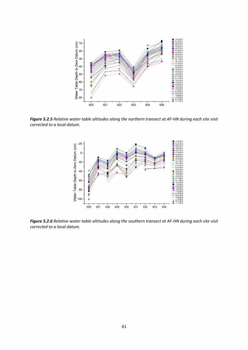
Figure 5.2.5 Relative water-table altitudes along the northern transect at AF-HN during each site visit corrected to a local datum.

Figure 5.2.6 Relative water-table altitudes along the southern transect at AF-HN during each site visit corrected to a local datum.

62

6. Somerset Levels

6.1 Tadham Moor – extensive grassland (SL-EG)

At SL-EG 12 manually recording dipwells were used to monitor the water-table. At each dipwell point a nest of piezometers was also installed with central intake depths of 40, 80, 120 and 160 cm from the surface (Figure 6.1.1). The dipwells were spread across three transects - one across the north of fen, one in the middle and one across the south of the fen. Water levels within the ditch running along the eastern edge of the fen were monitored using an automated logger.

Figure 6.1.1 Map of sampling points at SL-EG. Upper panel shows all sampling locations, bottom panel shows only dipwell locations.

ET data were taken from the onsite flux tower. An onsite rain gauge also provided precipitation data, however much of the record was missing. To gap fill the record, daily rainfall totals were obtained from four nearby stations to provide a daily average rainfall total and then summed to provide monthly totals (Table 6.1.1). These monthly totals compare well with the monthly totals from the COSMOS-UK station from November 2014 onwards (Figure 6.1.2). The site water-tables exhibited significant drawdown during summer months (Figure 6.1.3). When adjusted for topography there was limited variability in water-table altitude across the site although there was a slight doming with higher water-table altitudes toward the middle of the fen (Figure 6.1.4). Ditch water levels were typically below the water-table within the fen. Water export was typically limited to winter months, occurring

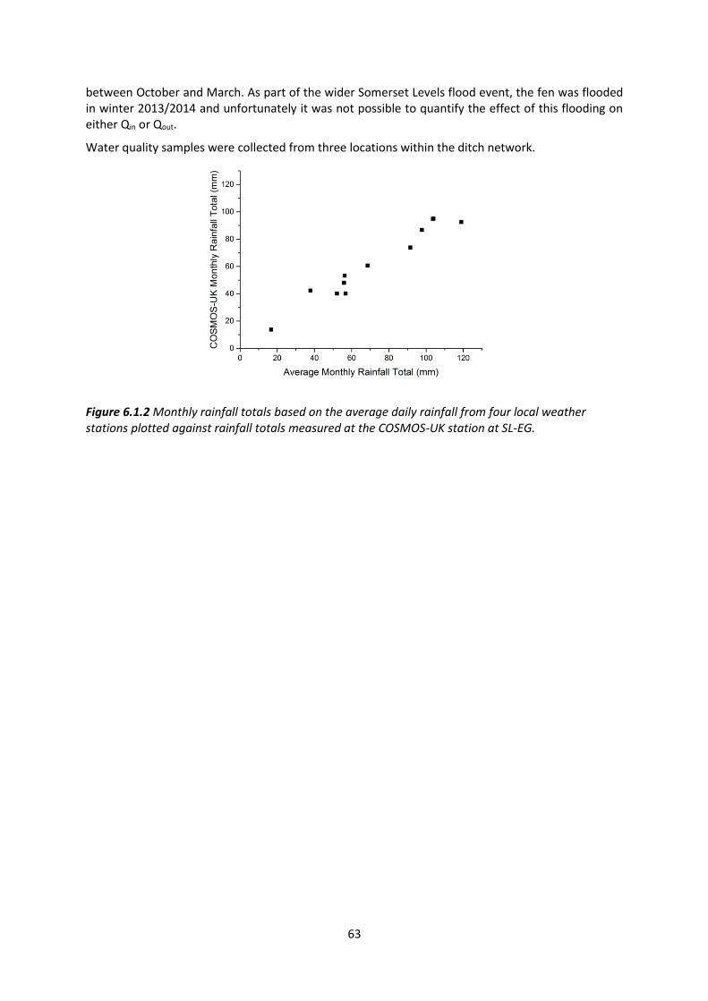
63

between October and March. As part of the wider Somerset Levels flood event, the fen was flooded in winter 2013/2014 and unfortunately it was not possible to quantify the effect of this flooding on either Qin or Qout.

Water quality samples were collected from three locations within the ditch network.

Figure 6.1.2 Monthly rainfall totals based on the average daily rainfall from four local weather stations plotted against rainfall totals measured at the COSMOS-UK station at SL-EG.

64

Table 6.1.1 Monthly water budget for SL-EG. Qout is the total aquatic loss from the site. Pnet based on

the average of four nearest met stations. Dark red shows months when flooding of the site occurred.

E Pnet Balance Qout

Oct-12 2.6 6.7 4.1 4.1

Nov-12 21.0 181.1 160.1 160.1

Dec-12 12.7 154.4 141.7 141.7

Jan-13 21.9 98.1 76.2 76.2

Feb-13 31.1 41.9 10.7 10.7

Mar-13 48.6 59.1 10.4 10.4

Apr-13 68.6 24.3 -44.3 0.0

May-13 106.9 59.1 -47.7 0.0

Jun-13 125.2 28.3 -96.9 0.0

Jul-13 115.6 37.1 -78.5 0.0

Aug-13 102.0 46.8 -55.2 0.0

Sep-13 63.0 48.3 -14.7 0.0

Oct-13 48.2 133.2 85.0 85.0

Nov-13 22.9 107.0 84.1 84.1

Dec-13 17.5 100.4 82.9 82.9

Jan-14 37.2 165.7 128.5 128.5

Feb-14 41.6 134.7 93.0 93.0

Mar-14 53.0 62.9 9.9 9.9

Apr-14 76.0 61.5 -14.5 0

May-14 113.3 92.9 -20.4 0

Jun-14 137.2 52.0 -85.2 0

Jul-14 124.9 31.8 -93.1 0

Aug-14 110.0 110.0 0.0 0

Sep-14 66.4 15.7 -50.7 0

Oct-14 42.8 89.0 46.1 46.1

Nov-14 21.9 95.1 73.2 73.2

Dec-14 22.7 48.0 25.3 25.3

Jan-15 28.1 86.8 58.7 58.7

Feb-15 25.4 60.6 35.2 35.2

Mar-15 48.1 40.2 -7.9 0

Apr-15 82.4 13.7 -68.7 0

May-15 109.2 73.8 -35.4 0

Jun-15 127.6 42.3 -85.3 0

Jul-15 106.7 92.6 -14.1 0

Aug-15 73.4 94.8 21.4 21.4

Sep-15 73.2 53.2 -20.0 0

Oct-15 35.1 40.2 5.1 5.1

Nov-15 29.7 71.4 41.6 41.6

Dec-15 28.1 76.2 48.1 48.1

65

Table 6.1.2 SL-EG monthly Qout, measured DOC, DIC, POC and dissolved CO2 and CH4 (mg l-1) and export of DOC, DIC, POC and dissolved CO2 and CH4 (g C m-2).



Apr-13 0 28.0 61.2 6.5 1.3 0.007 0 0 0 0 0

May-13 0 72.4 58.6 17.8 1.6 0.022 0 0 0 0 0

Jun-13 0 16 60.5 2.3 1.5 0.010 0 0 0 0 0

Jul-13 0 32.7 45.5 11.6 1.5 0.009 0 0 0 0 0

Aug-13 0 5.3 63.1 0.5 4.0 0.006 0 0 0 0 0

Sep-13 0 5.1 66.9 8.8 7.9 1.023 0 0 0 0 0

Oct-13 85.0 8.0 63.7 0.7 4.8 0.019 0.68 5.41 0.060 0.112 1.19E-03

Nov-13 84.1 62.0 28.3 1.3 19.2 0.081 5.21 2.38 0.109 0.441 5.14E-03

Dec-13 82.9 42.4 49.9 0.6 3.6 0.014 3.51 4.14 0.050 0.082 8.57E-04


Feb-14 93.0 n/a (C) n/a (C) n/a (C) n/a (C) n/a (C) n/a (C) n/a (C) n/a (C) n/a (C) n/a (C)

Mar-14 9.9 45.5 53.2 0.9 4.0 0.037 0.45 0.53 0.009 0.011 2.74E-04

Apr-14 0 33.2 58.5 0.8 4.5 0.064 0 0 0 0 0

May-14 0 20.7 65.1 0.6 3.5 0.017 0 0 0 0 0

Jun-14 0 20.3 63.1 1.8 1.8 0.033 0 0 0 0 0


Aug-14 0 9.3 53.7 4.7 n/a (C) n/a (C) 0 0 0 0 0

Sep-14 0 9.9 52.2 4.8 2.3 0.009 0 0 0 0 0

Oct-14 46.1 12.5 58.3 3.4 3.3 0.038 0.58 2.69 0.157 0.04 1.33E-03

Nov-14 73.2 19.7 59.5 0.7 8.9 0.076 1.44 4.36 0.051 0.18 4.16E-03

Dec-14 25.3 36.7 50.0 0.8 8.3 0.072 0.93 1.27 0.020 0.06 1.36E-03

Jan-15 58.7 36.5 49.4 0.3 15.8 0.150 2.14 2.90 0.018 0.253 6.60E-03

Feb-15 35.2 44.8 48.8 0.8 3.6 0.017 1.58 1.72 0.028 0.035 4.46E-04

Mar-15 0 39.4 58.3 1.1 2.5 0.025 0 0 0 0 0

Apr-15 0 33.8 65.6 3.5 0.9 0.037 0 0 0 0 0

May-15 0 10.0 57.1 6.4 0.9 0.051 0 0 0 0 0

Jun-15 0 8.8 59.3 4.4 5.5 0.033 0 0 0 0 0


Aug-15 21.4 12.3 59.5 n/a (C) 15.6 0.085 0.26 1.27 n/a (C) 0.090 1.36E-03

Sep-15 0 21.4 62.1 n/a (C) 10.3 0.727 0 0 0 0 0

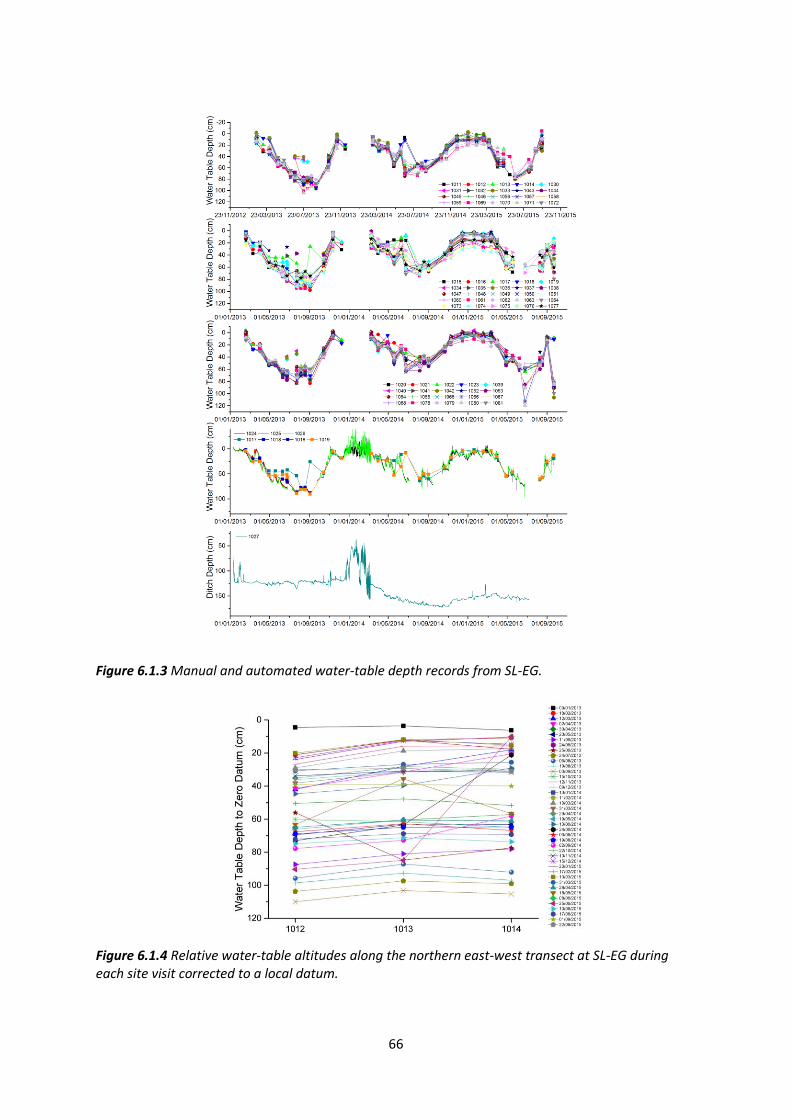
66

Figure 6.1.3 Manual and automated water-table depth records from SL-EG.

Figure 6.1.4 Relative water-table altitudes along the northern east-west transect at SL-EG during each site visit corrected to a local datum.

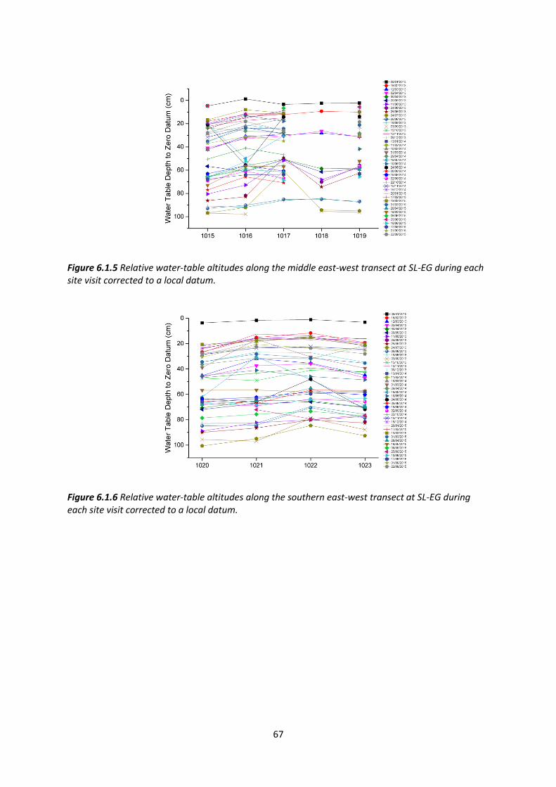
67

Figure 6.1.5 Relative water-table altitudes along the middle east-west transect at SL-EG during each site visit corrected to a local datum.

Figure 6.1.6 Relative water-table altitudes along the southern east-west transect at SL-EG during each site visit corrected to a local datum.

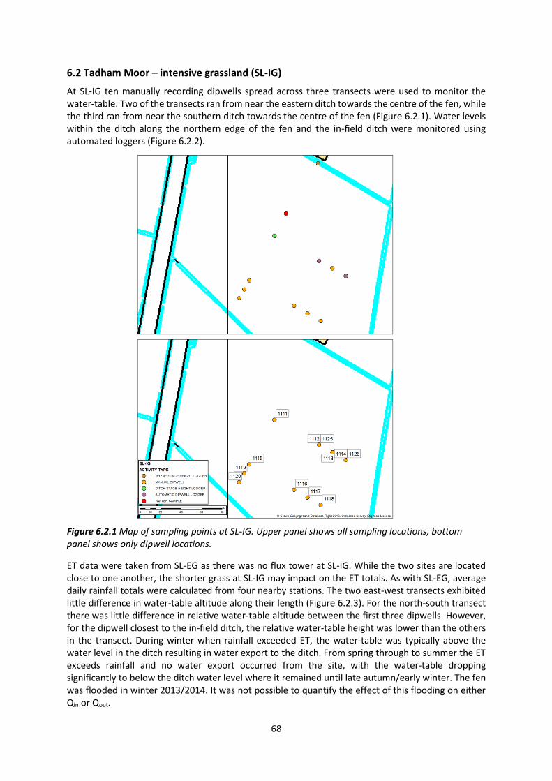
68

6.2 Tadham Moor – intensive grassland (SL-IG)

At SL-IG ten manually recording dipwells spread across three transects were used to monitor the water-table. Two of the transects ran from near the eastern ditch towards the centre of the fen, while the third ran from near the southern ditch towards the centre of the fen (Figure 6.2.1). Water levels within the ditch along the northern edge of the fen and the in-field ditch were monitored using automated loggers (Figure 6.2.2).

Figure 6.2.1 Map of sampling points at SL-IG. Upper panel shows all sampling locations, bottom panel shows only dipwell locations.

ET data were taken from SL-EG as there was no flux tower at SL-IG. While the two sites are located close to one another, the shorter grass at SL-IG may impact on the ET totals. As with SL-EG, average daily rainfall totals were calculated from four nearby stations. The two east-west transects exhibited little difference in water-table altitude along their length (Figure 6.2.3). For the north-south transect there was little difference in relative water-table altitude between the first three dipwells. However, for the dipwell closest to the in-field ditch, the relative water-table height was lower than the others in the transect. During winter when rainfall exceeded ET, the water-table was typically above the water level in the ditch resulting in water export to the ditch. From spring through to summer the ET exceeds rainfall and no water export occurred from the site, with the water-table dropping significantly to below the ditch water level where it remained until late autumn/early winter. The fen was flooded in winter 2013/2014. It was not possible to quantify the effect of this flooding on either Qin or Qout.

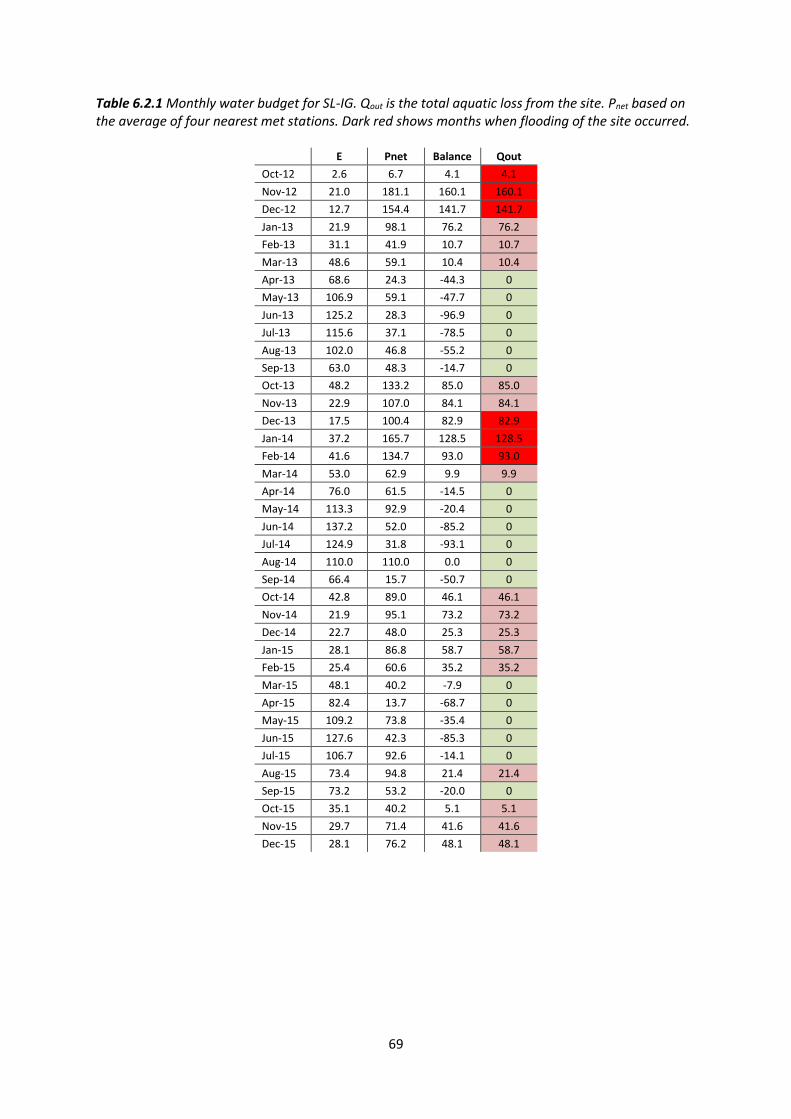
69

Table 6.2.1 Monthly water budget for SL-IG. Qout is the total aquatic loss from the site. Pnet based on the average of four nearest met stations. Dark red shows months when flooding of the site occurred.

E Pnet Balance Qout

Oct-12 2.6 6.7 4.1 4.1

Nov-12 21.0 181.1 160.1 160.1

Dec-12 12.7 154.4 141.7 141.7

Jan-13 21.9 98.1 76.2 76.2

Feb-13 31.1 41.9 10.7 10.7

Mar-13 48.6 59.1 10.4 10.4

Apr-13 68.6 24.3 -44.3 0

May-13 106.9 59.1 -47.7 0

Jun-13 125.2 28.3 -96.9 0

Jul-13 115.6 37.1 -78.5 0

Aug-13 102.0 46.8 -55.2 0

Sep-13 63.0 48.3 -14.7 0

Oct-13 48.2 133.2 85.0 85.0

Nov-13 22.9 107.0 84.1 84.1

Dec-13 17.5 100.4 82.9 82.9

Jan-14 37.2 165.7 128.5 128.5

Feb-14 41.6 134.7 93.0 93.0

Mar-14 53.0 62.9 9.9 9.9

Apr-14 76.0 61.5 -14.5 0

May-14 113.3 92.9 -20.4 0

Jun-14 137.2 52.0 -85.2 0

Jul-14 124.9 31.8 -93.1 0

Aug-14 110.0 110.0 0.0 0

Sep-14 66.4 15.7 -50.7 0

Oct-14 42.8 89.0 46.1 46.1

Nov-14 21.9 95.1 73.2 73.2

Dec-14 22.7 48.0 25.3 25.3

Jan-15 28.1 86.8 58.7 58.7

Feb-15 25.4 60.6 35.2 35.2

Mar-15 48.1 40.2 -7.9 0

Apr-15 82.4 13.7 -68.7 0

May-15 109.2 73.8 -35.4 0

Jun-15 127.6 42.3 -85.3 0

Jul-15 106.7 92.6 -14.1 0

Aug-15 73.4 94.8 21.4 21.4

Sep-15 73.2 53.2 -20.0 0

Oct-15 35.1 40.2 5.1 5.1

Nov-15 29.7 71.4 41.6 41.6

Dec-15 28.1 76.2 48.1 48.1

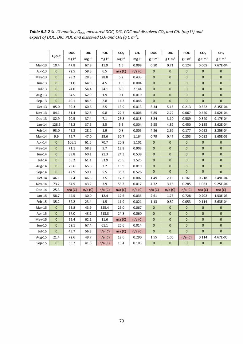
70

Table 6.2.2 SL-IG monthly Qout, measured DOC, DIC, POC and dissolved CO2 and CH4 (mg l-1) and export of DOC, DIC, POC and dissolved CO2 and CH4 (g C m-2).



Mar-13 10.4 47.8 67.9 11.9 1.6 0.098 0.50 0.71 0.124 0.005 7.67E-04

Apr-13 0 72.5 58.8 6.5 n/a (C) n/a (C) 0 0 0 0 0

May-13 0 28.2 28.3 28.8 5.2 0.433 0 0 0 0 0

Jun-13 0 51.0 64.9 4.5 1.0 0.004 0 0 0 0 0

Jul-13 0 74.0 54.4 24.1 6.0 2.144 0 0 0 0 0

Aug-13 0 34.5 62.9 1.9 9.1 0.019 0 0 0 0 0

Sep-13 0 40.1 84.5 2.8 14.3 0.046 0 0 0 0 0

Oct-13 85.0 39.3 60.6 2.5 13.9 0.013 3.34 5.15 0.213 0.322 8.35E-04

Nov-13 84.1 81.4 32.3 0.8 22.7 0.006 6.85 2.72 0.067 0.520 4.02E-04

Dec-13 82.9 70.5 37.4 7.1 23.8 0.015 5.84 3.10 0.589 0.540 9.17E-04

Jan-14 128.5 43.2 37.5 3.5 5.3 0.004 5.55 4.82 0.450 0.185 3.62E-04

Feb-14 93.0 45.8 28.2 1.9 0.8 0.005 4.26 2.62 0.177 0.022 3.25E-04

Mar-14 9.9 79.7 47.0 25.6 30.7 1.164 0.79 0.47 0.253 0.082 8.65E-03

Apr-14 0 106.1 61.5 70.7 20.9 1.101 0 0 0 0 0

May-14 0 71.1 58.3 5.7 13.8 0.903 0 0 0 0 0

Jun-14 0 89.8 60.1 21.3 24.3 0.539 0 0 0 0 0

Jul-14 0 65.2 61.1 53.9 25.5 1.525 0 0 0 0 0

Aug-14 0 29.6 65.8 3.2 13.9 0.019 0 0 0 0 0

Sep-14 0 42.9 59.1 5.5 35.3 0.526 0 0 0 0 0

Oct-14 46.1 32.4 46.3 3.5 17.3 0.007 1.49 2.13 0.161 0.218 2.49E-04

Nov-14 73.2 64.5 43.2 3.9 53.3 0.017 4.72 3.16 0.285 1.063 9.25E-04

Dec-14 25.3 n/a (C) n/a (C) n/a (C) n/a (C) n/a (C) n/a (C) n/a (C) n/a (C) n/a (C) n/a (C)

Jan-15 58.7 44.5 30.0 12.4 12.6 0.035 2.61 1.76 0.728 0.202 1.53E-03

Feb-15 35.2 32.2 23.4 1.5 11.9 0.021 1.13 0.82 0.053 0.114 5.63E-04

Mar-15 0 63.8 43.9 325.4 23.0 0.067 0 0 0 0 0

Apr-15 0 67.0 43.1 213.3 24.8 0.060 0 0 0 0 0

May-15 0 55.4 62.1 11.6 n/a (C) n/a (C) 0 0 0 0 0

Jun-15 0 69.1 67.4 61.1 25.6 0.014 0 0 0 0 0

Jul-15 0 45.7 56.3 n/a (C) n/a (C) n/a (C) 0 0 0 0 0

Aug-15 21.4 72.6 49.7 n/a (C) 19.6 0.290 1.55 1.06 n/a (C) 0.114 4.67E-03

Sep-15 0 66.7 41.6 n/a (C) 13.4 0.103 0 0 0 0 0

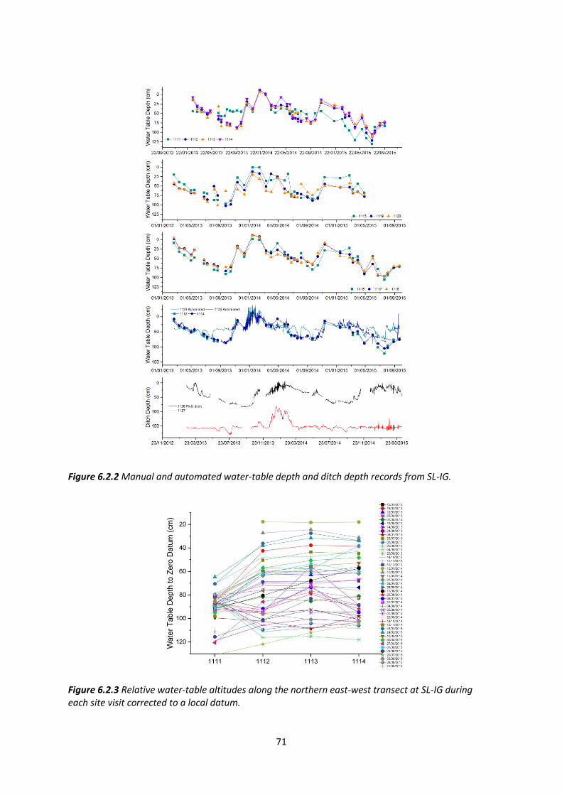
71

Figure 6.2.2 Manual and automated water-table depth and ditch depth records from SL-IG.

Figure 6.2.3 Relative water-table altitudes along the northern east-west transect at SL-IG during each site visit corrected to a local datum.

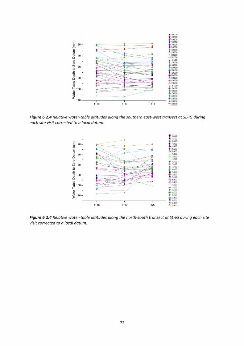
72

Figure 6.2.4 Relative water-table altitudes along the southern east-west transect at SL-IG during each site visit corrected to a local datum.

Figure 6.2.4 Relative water-table altitudes along the north-south transect at SL-IG during each site visit corrected to a local datum.

73

References

Finch, J.W., Hall, R.L. 2001 Estimation of Open Water Evaporation: Guidance for Environment Agency Practitioners. R&D Handbook W6-043/HB, Environment Agency, Bristol

Gilman, K., Newson, M.D. 1982 The Anglesey Wetlands Study. Institute of Hydrology, Wallingford, Oxon

Gilman, K. 1988. The hydrology of Wicken Fen. Final Report. NERC/Institute of Hydrology, 43pp.

Gilman, K. 1994 Hydrology and wetland conservation. Wiley-Blackwell. Chichester, UK

McCartney, M.P., de la Hera, A. 2004 Hydrological assessment for wetland conservation at Wicken Fen. Wetlands Ecology and Management, 12(3), 189-204.

McCartney, M. P., de la Hera, A., Acreman, M. C., Mountford, O. 2001 An investigation of the water budget of Wicken Fen. Wallingford, NERC/Centre for Ecology & Hydrology, 42pp. (CEH Project Number: C01538)

Scarlett, S. 2015 Characterizing controls on plot-scale evapotranspiration and soil water dynamics of a constructed fen in the Athabasca Oil Sands Region, Alberta. Unpublished MSc Thesis, University of Waterloo, Ontario

Stratford, C. Acreman, M. 2014 Somerset Levels and Moors: Assessment of the impact of water level management on flood risk. Report to Somerset Drainage Boards Consortium. Centre for Ecology and Hydrology

Thornthwaite, C.W. 1948 An approach toward a rational classification of climate. Geographical Review 38 (1): 55–94. doi:10.2307/21073

appendix 1. - gov.uk

Documents