A6.1-1

Appendix 6.1: Liquidity

Contents Page

Introduction ................................................................................................................ 1

Background ................................................................................................................ 2

Our assessment of liquidity ...................................................................................... 11

The relevance of liquidity to competition .................................................................. 30

Summary of the effects of the level of liquidity on competition ................................. 46

Introduction

1. In this appendix we discuss the levels of liquidity in GB wholesale electricity

trading, and its effects on competition. We also discuss some aspects of

wholesale gas trading, as it may be a useful comparator in some ways. Some

of our detailed analysis is presented in an annex, and summarised in the main

body of this appendix.

2. The relevant theory of harm (3a) in our updated issues statement was that

‘opaque prices and low liquidity in wholesale electricity markets distort

competition in retail and generation’.1

3. Our primary concern about the level of liquidity is therefore whether it is

sufficiently low that it distorts competition in relevant markets. This is most

likely to occur if some parties are less able than others to: (a) ‘hedge’ their

demand or supply (ie contracting wholesale electricity in advance of delivery

as protection against spot price changes);2 and/or (b) balance their position at

delivery. If so, it could place certain suppliers or generators at a competitive

disadvantage and/or act as a barrier to entry or expansion.

4. In this appendix, first we explain what we mean by liquidity, explain how

wholesale electricity is traded, and give some background on previous

regulatory investigations and interventions in this area.

5. We then assess the level of liquidity in the market by considering appropriate

metrics and gathering data from suppliers, generators and brokers. We

explain how poor liquidity could distort competition, and especially how it

could benefit VI firms at the expense of other firms. We go on to assess the

likely effects of liquidity on competition, primarily by examining evidence on

1 Updated issues statement. 2 See paragraph 103 for a full discussion of our use of the word ‘hedging’ in this paper.

Annex ....................................................................................................................... 47

A6.1-2

the hedging strategies of various parties and the role of liquidity in the

implementation of these strategies.

Background

6. In this section we first define what we mean by liquidity (paragraphs 8 to 14).

We then describe how wholesale electricity and gas are traded in GB markets

(paragraphs 15 to 20). We comment on the extent to which liquidity in

electricity and gas can be compared, and why gas is generally held to be

more liquid (paragraph 21).

7. We then give a brief overview of recent regulatory investigations and

interventions into electricity liquidity, notably Ofgem’s recent introduction of

Secure and Promote (S&P) licence conditions (paragraphs 23 to 27). We

summarise parties’ views on liquidity (paragraphs 29 to 32). Finally, in this

section, we explain why near-term liquidity is not a focus of our investigation

(paragraphs 34 to 35).

What is liquidity?

8. Generally, liquidity is a measure of the availability of an asset to a market or

company. More precise definitions are elusive, perhaps because liquidity can

have different meanings in different contexts.

9. Ofgem has defined liquidity in wholesale energy markets as ‘the ability to

quickly buy or sell a desired commodity or financial instrument without

causing a significant change in its price and without incurring significant

transaction costs’. Ofgem has also noted that a feature of a liquid market is

that it has a large number of buyers and sellers willing to transact at all times,

and this facilitates product availability and price discovery.3

10. For the purposes of this appendix, we use a relatively narrow definition of

liquidity. We want to focus on those aspects of liquidity that are common to

market participants – we might describe this as product availability. In effect,

we are assessing whether the market offers products that parties want to

trade, whether these products are available in ‘reasonable’ quantity, and

whether prices are well defined. In other words, in a liquid market for a

particular product, parties will have a reasonable expectation that they could

buy (or sell) a ‘reasonable’ quantity without affecting the price. In a liquid

market, parties are able to engage in trading with the reassurance that they

3 Ofgem (June 2009), Liquidity in the GB wholesale energy markets, paragraphs 1.8 & 1.9.

A6.1-3

would also be able later to sell back to (or buy back from) the market at a

similar price, unless new information has justifiably caused prices to change.

11. We do not include in our definition or analysis in this appendix factors that

may vary from party to party – for example, posting collateral on trades, where

the amount of collateral will depend on (among other factors) the party’s credit

rating; or the amount a party can trade with any particular counterparty. We

do not look at transaction costs under the heading of liquidity.4 Therefore, our

definition is narrower than Ofgem’s.

12. There are a number of dimensions to trading in electricity. These dimensions,

which give rise to a wide range of wholesale electricity products, include:

(a) the delivery start date (we often refer to trading ‘ahead of delivery’, or

trading ‘along the curve’ – by ‘further along the curve’ we mean a greater

time ahead of the start of delivery);

(b) duration of delivery (eg on a single day; or for every day in a Month, a

Quarter, a ‘Season’ (six months) or a year);

(c) hours of delivery (eg ‘Baseload’, which delivers all day; a 12-hour ‘Peak’

period on weekdays; four-hour ‘Blocks’; or a single half hour); and

(d) clip size (ie the size of the product in capacity terms).

13. This means that a single product (eg 10MW of Peak in June 2015) could

potentially be traded at any time from several years ahead to just before the

start of delivery, and it may be more liquid at certain points in time (typically

closer to delivery). It also means that a unit of electricity delivered at a

particular time could be included in any number of products. Therefore, for

example, a party could trade a Quarterly product or a ‘strip’ of the three

equivalent Monthly products and receive exactly the same delivery, but the

Quarterly product may be more or less liquid than the three Monthly products.

14. This leads to some fragmentation of products. In particular, the electricity day

is broken into 48 half-hour periods that can be traded individually. This

contrasts with the gas market, where the smallest unit is a whole day. The

most widely traded product types are Baseload and Peak for Seasons,

Quarters or Months. Industry participants often refer to ‘shape’, which tends to

mean either ‘daily shape’ (hours of delivery more granular than Peak to reflect

the fact that demand varies over the course of the day) or ‘annual shape’

4 We do look at bid-offer spreads, which could be viewed as a transaction cost. We view these spreads as a measure of product availability.

A6.1-4

(relatively short durations of delivery – generally months or less – to reflect the

fact that demand is seasonal).

How are wholesale electricity and gas traded?

15. Parties have several choices about how to trade wholesale electricity and gas

products. The two main routes for trading electricity and gas futures5 are

brokered over-the-counter (OTC) and exchanges:

(a) Brokered OTC bilateral trades in futures are agreements to supply a

particular volume of gas or electricity at a particular time. The majority of

electricity trades take place via a small number of brokers6 using a

screen-based system provided by Trayport. Trading is continuous through

the day. Parties post bids and offers, the brokers anonymise them, and

one party may trade with another only if it has a trading agreement and

the trade is within the parties’ agreed credit limits.7

(b) N2EX and APX are the main exchanges where electricity is traded, and

contracts on these exchanges are short term.8 Much of this trading occurs

through auctions at the day-ahead stage. ICE is a third exchange, but little

trading in futures contracts takes place on it. GB power contracts are also

listed on the Nasdaq OMX exchange.

16. There are also some direct bilateral trades and long-term contracts between

parties that are not visible to the market. VI firms may also trade internally,

and this will be similarly invisible to the market. Also, a party may employ an

intermediary to trade on its behalf, rather than trading with the market

directly.9

17. The Electricity Supply Board (ESB, a generator operating in GB and the

Republic of Ireland) submitted analysis of publicly visible electricity trades.

This showed that in 2013 (the most recent full year), 84.1% of volumes traded

took place OTC via brokers, 14.9% via N2EX and the remainder via APX and

ICE. This is broadly consistent with our analysis of the trading of 16 firms,

5 While the distinction between ‘futures’ and ‘forwards’ may be relevant in other contexts (eg financial regulation), this paper uses the term ‘futures’ to refer to both types of products. 6 Until recently there were four; now there are five. More brokers are active in gas. 7 A Grid Trade Master Agreement (GTMA) sets out the terms on which two parties can trade. The software will make each party aware of whether it can take up a particular bid or offer, but does not reveal the identity of the counterparty until the trade is completed. 8 N2EX provides its members with access to a market coupled day-ahead auction. APX provides its members with access to a market coupled day-ahead auction, an intraday market for half-hourly products, a market for prompt products up to two days in duration and a day-ahead auction for half-hour products. 9 We discussed some of the specific arrangements that independent firms have with intermediaries further in our case studies on Retail barriers to entry and expansion.

A6.1-5

which showed 81.2% by volume taking place OTC through brokers, 13.3% via

exchanges and 5.5% via direct bilateral trades.10

18. Some suggestions have been made that the wholesale energy markets lack

transparency.11 The figures above suggest that the large majority of external

trading takes place via platforms where prices are transparent to any industry

participant, or indeed any interested party willing to obtain a subscription.12

This should be sufficient to give good price signals to any party interested in

making investment decisions or planning energy trades. It should be noted,

however, that the identities of parties and thus the costs of energy trades

actually paid by individual parties do remain confidential.

19. VI firms engage in internal trading, and these prices are not reported to the

market. It is difficult to measure the extent of internal trading: some of it takes

the form of arm’s-length trades comparable to external trades, but some VI

firms also trade generation capacity rather than volume, or transfer between

‘books’. This might be a concern if VI firms conducted little external trading,

but all of them externally trade multiples of their output and demand;13 this

should be sufficient for them to play a role in price formation.

20. Price reporting agencies also play a role in the market: they validate and

research trading data to produce price indices and carry out their own

assessments of market prices. They carry out these activities with reference

to their published methodologies, and make them available to subscribers.

These agencies also contribute to the communication of industry data to those

without a day-to-day interest in energy markets.

Comparability of electricity and gas

21. The trading of wholesale gas in GB is generally held to be relatively liquid,

and certainly more so than the trading of electricity. There are several

possible reasons for this:

(a) It is more practicable to store gas than electricity; and electricity needs to

match supply to demand within narrow margins at each moment, whereas

gas needs only to maintain pressure within much wider margins. The

10 This excludes cash-out, which represents a small proportion of most firms’ volumes. 11 For example, Which? (July 2013), The imbalance of power: wholesale costs and retail prices, p28. 12 For example, Trayport provides software which allows firms to use, view and manage market data from a variety of sources (including platform operators). (Market participants do not need a commercial relationship with Trayport to view or trade prices.) Trayport’s licence fee for a single read-only screen that would allow (with permission from platform operators), for example, a small supplier to see all GB power and gas market trades executed on those platforms would be between £[] per month. Opus told us that it has ‘read-only access to all the primary trading platforms used to trade electricity so that we can monitor the wholesale market prices’, which shows that this is used in practice. 13 See Table 2 below.

A6.1-6

consequences of this are that electricity is traded in half-hour periods and

parties are incentivised to match their supply with demand before the start

of each period, whereas gas is traded in daily (24-hour) periods and

parties can balance supply and demand within each period.

(b) Fragmented products: as a result of the above, there are 48 times as

many basic products for electricity as there are for gas. These products

can then be combined in any number of ways, so the market tends to

adopt conventions to standardise product definitions. There is still a large

number of potential products, so it is natural for liquidity to concentrate

around certain popular products (particularly along the curve).

(c) International links: the GB electricity system is connected to those of

Ireland, France and the Netherlands. However, the level of

interconnection in GB is low, particularly compared to other European

markets.14 In contrast, the GB gas market is a hub with a range of

external supply sources (upstream production, interconnectors and

liquefied natural gas imports). This creates a range of trading

opportunities, and makes it an attractive market for participants across

Europe.15 A recent study by the Agency for the Cooperation of Energy

Regulators (ACER) showed that the British and Dutch gas markets

performed significantly better than other European gas markets against a

range of wholesale market metrics.16

(d) VI: electricity exhibits a high degree of VI, with some internal trading that

is never seen or recorded by markets taking place. The degree of VI in

gas is much lower. To the extent that VI firms trade internally, a certain

amount of liquidity may be removed from external markets (although all of

the Six Large Energy Firms trade multiples of their generation and

demand in electricity).

(e) Regulatory uncertainty: several parties told us that there was uncertainty

over the future level of the Carbon Price Floor, which has a substantial

impact on electricity prices. Therefore, it was not attractive to trade in

electricity products beyond the time horizon at which the level of the floor

is set.17 In contrast, gas is not affected by this. Therefore, financial activity

14 See Section 4: Nature of wholesale competition. 15 E.ON told us that ‘many companies across Europe trade NBP as a proxy for their own needs’. 16 ACER (January 2015) European gas target model review and update, Figure 3. 17 E.ON told us that this policy adversely affects liquidity in two ways: first, through uncertainty as to the level of the tax that is set in the government’s Budget each year for the tax year two years ahead, which means that generators have to take a higher risk in selling their output more than two years ahead, thus requiring a significant risk premium to sell output forward and also dampening the incentive for any supplier to buy on this timescale; and second, through the distortion the tax has caused in the differentials in costs between generation

A6.1-7

(speculation) would be attracted to gas in preference to electricity.18 More

generally, it has been suggested that the gas market has benefited from

greater regulatory and policy stability. In addition, Ofgem said that the

perceived and actual regulatory risk stemming from the various strands of

European financial legislation (such as MiFID II) also discouraged

financial players.

(f) Ofgem also said that the returns available in a market that lacked price

volatility were perceived to be low. It said it had been told that, in a period

in which financial players had constrained risk capital, GB electricity

trading was unlikely to be a high priority.

22. We acknowledge that the fundamental differences between gas and electricity

mean that it would not be reasonable to set liquidity in gas as the benchmark

against which to judge liquidity in electricity. Nevertheless, since many of the

same parties are involved in both markets, we find it instructive at certain

points to draw comparisons.

Regulatory interventions – Secure and Promote

23. Ofgem and the DECC have previously assessed liquidity in GB. During

Ofgem’s 2008 investigation into energy supply (‘the Probe’), small suppliers

and potential new entrants highlighted the lack of liquidity in the wholesale

electricity market and raised concerns about the functioning of the market

itself. Ofgem decided that action was needed to address these concerns.19 In

2009 it published a discussion paper20 that found that liquidity in electricity in

GB was lower than in other energy and commodity markets, including a

number of European electricity markets. The report analysed a range of

factors that had contributed to the low level of liquidity in GB electricity, and

outlined possible policy options that could improve liquidity.

24. As part of this process, Ofgem developed three liquidity objectives:21

(a) improved availability of products to support hedging;

in GB and continental Europe, which has impacted flows across the interconnector E.ON noted that it also had other concerns about higher regulatory uncertainty in electricity compared to gas. 18 For example, SSE said: ‘The Carbon Price Floor has had a negative impact on long-term liquidity due to uncertainty around future levels, which can be changed at every budget … Why would a hedge fund choose to trade forward power (the value of which could be materially affected by a sentence of the Chancellor’s speech on carbon taxation) when they can take equivalent commodity price risk in the UK gas market where none of the peripheral political risk exists?’ 19 Ofgem (October 2008), Energy supply probe: initial findings report, paragraph 1.34. 20 Ofgem (June 2009), Liquidity in the GB wholesale energy markets. 21 Ofgem (22 February 2012), Retail market review: intervention to enhance liquidity in the GB power market,

Figure 3.

A6.1-8

(b) robust reference prices along the curve (prices along the forward curve

that are trusted to provide a fair reflection of the value of products – these

prices provide valuable signals for market participants); and

(c) an effective near-term market (so firms can avoid imbalance).

25. By 2013, Ofgem considered that the third of these objectives was being met,

even though it had not made any direct interventions. However, it still had

outstanding concerns about the first two objectives relating to forward mar-

kets.22 After further reports and consultations, Ofgem introduced the S&P

licence conditions,23 which came into effect on 31 March 2014.

26. The S&P conditions have three distinct elements: Supplier Market Access

rules; Market Making obligations; and reporting requirements.

(a) The Supplier Market Access rules oblige the eight largest generating

companies24 to consider applications for trading agreements from smaller

suppliers (defined by size) within specified time frames.25

(b) Under the Market Making obligations the Six Large Energy Firms must

offer to trade certain products (buy and sell with prescribed maximum

spreads) in two hour-long windows every day. These products are:

(i) Baseload: Month+1, Month+2, Quarter+1, Season+1, Season+2,

Season+3, Season+4; and

(ii) Peak: Month+1, Month+2, Quarter+1, Season+1, Season+2,

Season+3.

(c) The reporting requirements imposed on the eight specified firms enable

greater monitoring of the near-term market by the regulator. Ofgem

published an interim report on S&P in December 2014.26 Ofgem stressed

that it would need to see the licence condition in operation for longer, in

22 Ofgem (12 June 2013), Wholesale power market liquidity: final proposals for a ‘Secure and Promote’ licence condition, Figure 1. 23 Generation Special Licence Conditions AA. 24 The Six Large Energy Firms plus Drax and GDF Suez. 25 The key requirements are to:

consider applications for trading agreements from smaller suppliers within specified timeframes;

offer proportionate credit and collateral terms;

provide transparency, both in relation to the information required to open negotiations on a trading agreement, and in relation to the rationale for the credit terms offered; and

offer to buy and sell a defined list of products with smaller suppliers (once a trading agreement is in place). The products must be available in small clip sizes, and generators are allowed to add only specific elements to the market price.

26 Ofgem (18 December 2014), Wholesale power market liquidity: interim report.

A6.1-9

order to have sufficient data to identify its effects.27 It also noted that a

variety of other factors could have affected liquidity in the period, such as

increases in the spark spread.28 Ofgem observed that:29

Our analysis shows that there has been some improvement in

liquidity since Secure and Promote was introduced. Several

independent suppliers have also told us that it is easier for

suppliers and generators to access the products they need and

that prices for those products are perceived by industry as

more robust during the times when market making takes place.

In addition, trends such as increasing churn (the electricity

traded compared to the amount delivered to consumers) and

falling bid–offer spreads (the difference between the buy and

sell price for a product) show that liquidity is improving.

Many factors can impact liquidity and it is difficult to isolate the

effect of our reforms. In addition, liquidity follows seasonal

trends. While there are positive signs so far, it is too early to

draw more meaningful conclusions. At least a full year of data

is needed.

27. Based on feedback from stakeholders, Ofgem reported that independent

suppliers were finding it easier to access products under the Supplier Market

Access rules.30 However, independent suppliers were still finding credit and

collateral to be an issue.31

28. We make some observations on the effects of S&P below (from paragraph

76), although we recognise that it is too early to draw robust conclusions on

its implications for liquidity as a whole, and note that Ofgem will continue to

monitor its effects on liquidity.

Parties’ views on liquidity

29. We give parties’ views on liquidity in detail in the Annex, and summarise them

here.

30. The Six Large Energy Firms generally shared the view that liquidity was

sufficient for their purposes, although all of them noted (either in their

responses to our consultation or in internal documents) that it was limited in

27 Ofgem (18 December 2014), Wholesale power market liquidity: interim report, p5. 28 Ofgem (18 December 2014), Wholesale power market liquidity: interim report, paragraph 1.14. 29 Ofgem (18 December 2014), Wholesale power market liquidity: interim report, pp4–5. 30 Ofgem (18 December 2014), Wholesale power market liquidity: interim report, paragraph 2.3. 31 Ofgem (18 December 2014), Wholesale power market liquidity: interim report, paragraph 2.3.

A6.1-10

some products and/or if it is possible to improve liquidity in some products it

would be to the benefit of all market participants.

31. Some, but not all, independent suppliers believed that liquidity was sufficiently

low, at least in particular products, as to impose additional risk and/or costs on

them ([], First Utility, [], Ecotricity). At least one (First Utility) also told us

that it placed vertically integrated suppliers at a competitive advantage

because they could trade internally even when products were not available, or

when there was no confidence in prices, in externally traded markets. By

contrast, Utility Warehouse told us that more than sufficient liquidity was

available.

32. Independent generators including Drax, ESB and InterGen all told us that

there were limits to liquidity that affected their businesses. However, Drax said

that the lack of shape trading until close to delivery is because it is

inconvenient for generators to trade non-standard products, and because

suppliers’ demand becomes more predictable closer to delivery.

33. The general view was that liquidity is good in the gas market. This opinion

was held by both the Six Large Energy Firms and independent suppliers.

However, several parties said that liquidity was lower towards the end of the

curve and that liquidity in Monthly products declined over time.

Near-term liquidity

34. We did not look in detail at near-term liquidity (ie trading on the day of delivery

and day ahead). Our understanding based on Ofgem’s work and response to

our issues statement is that liquidity here is good, and sufficient to allow firms

to balance their positions. The volume traded on day-ahead auctions is one

indicator of how well the near-term market is performing, and this has

increased substantially in recent years – see Figure 1, below. Ofgem noted in

201232 that a number of market developments had contributed to near-term

market liquidity: namely, that all of the Six Large Energy Firms had committed

to trading on a day-ahead auction; that intra-day market offerings were

deemed to be sufficient; and that GB market coupling via the ‘virtual hub’ was

likely to enhance near-term liquidity (day-ahead market coupling with north-

west Europe was introduced in February 2014).

32 Ofgem (July 2012), Retail market review: GB wholesale market liquidity update (letter to stakeholders).

A6.1-11

Figure 1: Day-ahead auction trading volumes (APX and N2EX)

Source: Ofgem (November 2013), Wholesale power market liquidity: statutory consultation on the ‘Secure and Promote’ licence condition – impact assessment, Figure 13 (based on data from APX, N2EX).

35. We did not receive any comments from parties suggesting concerns about

near-term liquidity; nor have we seen any evidence during our investigation to

date that this should be a concern. Therefore, we have focused our analysis

on liquidity in products for delivery further ahead.

Our assessment of liquidity

36. There is no single measure of liquidity, and no clear standard by which a

market is judged to be liquid. Some widely used measures are:

(a) volume or number of trades – this can be aggregate or of individual

products. In our analysis we have identified commonly traded products

and analysed the volume that is traded in various periods of time ahead of

delivery;

(b) churn – this is the ratio of volumes traded to volumes consumed. It is

usually reported as an aggregate measure, although it is also possible to

take a ratio of a particular product to total volumes consumed;33

(c) spreads – this looks at the difference between the buy price and the sell

price of a particular product at a particular time. Generally, the smaller the

33 It would not be meaningful to try to split volumes consumed into different products, so this type of measure would generally be used to compare products rather than to say anything about aggregate trading.

A6.1-12

spread, the more liquid a product is, because parties can both buy and

sell at similar prices, and prices are well defined. It can be used to look at

the availability of products (eg if there is little trading but tight spreads, this

might suggest a lack of demand rather than a lack of availability); and

(d) depth – we consider availability and spreads at different depths. It may be

possible to buy and sell small quantities at tight spreads, but a party

wishing to trade larger quantities may not be able to do so, or may face

significantly worse prices.

37. As noted above, our primary concern about the level of liquidity is whether it

distorts competition in relevant markets, and in particular whether some

parties are less able than others to hedge their demand or supply in advance

of delivery. As a result, we have placed less emphasis on churn, because:

(a) it is a market-wide indicator; and (b) it is not clear what different levels of

churn imply for this question. We are more interested in statistics that will give

us an insight into availability for different products at different points in time

ahead of delivery (including spreads and depth).

38. We present detailed results of our analysis in the Annex, and summarise them

below. First, we look at the volume of actual trading of particular firms for

which we had good data (paragraphs 39 to 47). We also compare this with

gas data, since we think the results are instructive (paragraphs 48 to 51).

Second, we briefly summarise findings on churn (paragraphs 52 to 53). Third,

we look at the availability of products to be traded via brokers (spreads and

depth) (paragraphs 54 to 75). Fourth, we look at the effects of S&P in its first

months of operation (paragraphs 76 to 96). We then set out our analysis of

the state of liquidity in wholesale electricity (paragraph 99).

Volume of trading

39. We asked a number of suppliers and generators (including VI firms) for details

of their external trades for delivery of electricity in the period January 2011 to

July 2014. We categorised these products for the purposes of analysis in

three ways: by time ahead of delivery, by duration, and by product type, and

grouped them by type (see Table 1).

A6.1-13

Table 1: Categorisation of trades

Category Product types What does this provide? Applies to gas?

Time ahead of delivery Over 36 months ahead, 24 to 36 months ahead, 12 to 18 months ahead, six to 12 months ahead, three to six months ahead, one to three months ahead, one week to one month ahead, one day to one week ahead, day ahead or less

Volumetric hedge Yes

Duration Beyond Season, Season (six months), Quarter, Month, Week, one day to one week, one day or less, other

Annual shape Yes

Product type Half-hour, Hour, Half Block (two hours), Block (four hours), Two Blocks (eight hours), Peak, Extended Peak, Off-Peak, Baseload, Custom, other

Daily shape No

40. This data does not cover the entire market, and does not include internal

trades for VI firms, but we believe we have sufficient coverage to give us a

good view of trading behaviour.34

41. Over the last three years, each of the Six Large Energy Firms traded multiples

of the size of their final consumption and generation, and therefore made a

net contribution to liquidity (see Table 2). The lowest trading multiple was [],

indicating that it traded twice as much as the sum of its generation and

consumption.

Table 2: Average annual traded volume and physical volume (generation plus consumption)

Centrica E.ON

EDF Energy

RWE Scottish

Power SSE

Average annual traded volume (TWh)

[] [] [] [] [] []

Average size of physical business (TWh)

[] [] [] [] [] []

Trading multiple [] [] [] [] [] []

Source: Physical volumes from Ofgem segmental statements; parties’ trading data; CMA analysis. Notes: 1. Annual average traded volume is based on all trades delivering in the period January 2011 to July 2014. Sleeve trades have been removed where possible. 2. Average size of physical business is based on Ofgem segmental statements for 2011–2013. We used the supply volumes as reported in the segmental statements (after losses) – adjusting for losses would not have a material effect on this table.

42. Looking at overall volumes, we found that the majority of trading by the Six

Large Energy Firms is within a year ahead of delivery, and this pattern is

consistent between firms. However, the volumes traded towards the far end of

the curve can still be significant. For example, Centrica traded nearly [] per

year over three years ahead of delivery. This is only [] of Centrica’s external

trading, but, for comparison with the needs of an independent supplier, []

consumption was [] TWh in the year from August 2013 to July 2014. This

34 Our data covers the following parties: Centrica, E.ON, EDF Energy, RWE, Scottish Power, SSE, Co-op Energy, Ecotricity, First Utility, OVO Energy, Utilita, DONG Energy, Drax, ESB, GDF Suez and MPF.

A6.1-14

indicates that the volumes traded in the market even far down the curve are

large, relative to the current size of independent suppliers.

43. The independent suppliers for whom we had data traded very limited volumes

more than a year before the start of delivery. In general, they traded nearer to

delivery than the Six Large Energy Firms. We observed a similar result for

independent generators.

44. We looked at specific products and types of product. First, we compared

Seasonal (six-month), Quarterly and Monthly products, focusing on Baseload

and Peak products, as the two main product types for these durations. We

found that Seasonal Baseload is traded along the curve, with some trading

more than three years ahead of delivery. We observed that, by contrast,

trading of Monthly Baseload is concentrated within three months of delivery

(some parties traded small amounts of Monthly Baseload beyond six months

ahead), with much lower volumes than the Seasonal product. Quarterly

Baseload is traded slightly more three to six months out, but very little beyond

that. There is a similar pattern for Peak – Seasonal products are traded much

further ahead than Monthly or Quarterly products. For Monthly Peak products,

the amount of activity beyond three months ahead is very small.

45. We then looked at daily shape. Having already looked at Peak products, we

turned our attention to Block products.35 Among the Six Large Energy Firms,

the majority of trading in these products was closer to delivery – each firm

traded at least 70% of its volume in these products within three months out.

All firms carried out some trading more than a year ahead, although only two

firms did so in larger volumes along the curve. Independent suppliers and

independent generators also generally traded these products within three

months of delivery.

46. We combined the trades made by all of the parties in our data set and looked

at how the volume was split between products and over time. The results are

presented in Table 3. We do not claim that this is necessarily representative

of all trading, but we have sufficient coverage that it should give a reasonable

indication.36 Over 50% was Seasonal Baseload, and much of this was traded

well in advance of delivery. There was very little trading in Quarterly, Monthly

and other products more than six months from delivery: only 2.3% of trading is

both more than six months out and not in Seasonal products. Less than a

month from delivery, trading switches predominantly to other products as

35 We are looking here at four-hour Blocks, and combinations of these Blocks (eg Overnights), but excluding Peak, as this was considered above. The amount of trading on products smaller than a four-hour Block is very small until shortly before delivery. 36 Note that some trades will be included twice in our data, if they are conducted between two firms in our data set. However, we have no reason to think that this should cause bias.

A6.1-15

forecasts of demand are refined and firms seek to shape their demand and

output.

Table 3: Split by product type of electricity volumes traded by energy firms in our data set

%

Seasonal Baseload

Quarterly Baseload

Monthly Baseload

Seasonal Peak

Quarterly Peak

Monthly Peak Blocks* Other

Total (sum of

columns)

Over 2 years 3.8 0.0 0.0 0.0 0.0 0.0 0.0 0.1 4.0 1–2 years 12.8 0.0 0.0 0.3 0.0 0.0 0.3 0.7 14.2 6–12 months 13.5 0.3 0.1 0.8 0.0 0.0 0.3 0.5 15.5 1–6 months 17.2 5.2 3.9 1.0 0.3 0.2 0.9 0.9 29.7 Less than 1 month 2.9 1.4 7.1 0.2 0.0 0.4 3.5 21.0 36.6

Total (sum of rows) 50.3 6.9 11.2 2.3 0.4 0.6 5.1 23.2 100.0

Source: CMA analysis, parties’ data (the Six Large Energy Firms, Co-op Energy, Ecotricity, First Utility, OVO Energy, Utilita, DONG Energy, Drax, ESB, GDF Suez, MPF). *Blocks include all combinations of standard Blocks, apart from standard Peak products.

47. Products covered by the S&P market making obligation accounted for 64% of

trading by volume (among parties whose data we have analysed). Excluding

products for delivery within a month, these obligated products accounted for

83% of trading by volume.

Comparison to gas

48. We asked relevant parties for equivalent data on their gas trading. This data is

somewhat simpler since it does not have the time-within-day dimension; but it

is otherwise comparable. As noted above, there are a number of differences

between electricity and gas, which mean that we should not use gas as a

simple benchmark by which to judge electricity (ie a finding that gas is in any

sense ‘more liquid’ than electricity does not itself imply that there is a problem

in electricity liquidity).

49. We found that most gas trading by the Six Large Energy Firms was within a

year from delivery. This pattern of when they traded was similar to electricity.

However, they traded greater volumes (relative to consumption), so the

absolute volumes that they traded along the curve were large, relative to

electricity. Most trading by independent suppliers was within a year from

delivery.

50. We found that the Six Large Energy Firms generally traded Monthly products

within three months of delivery – the same as for electricity. Their trading

beyond this therefore took the form of Quarters or Seasons. By contrast most

independent suppliers in our data traded Monthly products as far out as they

traded any products. However, these firms had agreements with a range of

trading partners that may have permitted them to access products that were

A6.1-16

not necessarily traded in the market at the time, with the intermediary taking

on the risk (eg Shell told us that it does so on request).

Table 4: Split by product type of gas volumes traded by energy firms in our data set

%

Seasons Quarters Months Other Total (sum of

columns)

Over 2 years 3.8 0.0 0.2 0.3 4.3 1–2 years 9.7 0.2 0.7 0.1 10.7 6–12 months 12.1 0.9 1.7 0.1 14.8 1–6 months 20.2 6.5 8.1 0.3 35.1 Less than 1 month 3.6 1.5 18.7 11.2 35.1

Total (sum of rows) 49.4 9.1 29.4 12.0 100.0

Source: CMA analysis, parties’ data (Co-op Energy, Ecotricity, First Utility, Utilita).

51. Table 4 shows the split of aggregate gas volumes traded by the companies in

our data (analogous to Table 3’s electricity volumes).37 Compared with

electricity, we see a little more trading in Quarters and Months more than six

months from delivery, but the proportions are still relatively small: only 4.2% of

trading is both more than six months out and not in Seasonal products.38 By

comparing the ‘total’ rows and columns between the two tables, we see that

patterns of trading by time ahead of delivery are very similar for gas and

electricity: if anything, electricity trades slightly further ahead of delivery than

gas. This is opposite to the result we would expect if liquidity in electricity

were a concern. The main difference between the two tables is within one

month of delivery, where there is a considerable amount of trading of Monthly

gas products whereas more electricity trading is in ‘Other’. This is likely to

reflect the greater granularity of electricity products and the need to trade daily

shape. We do not see anything in this comparison to suggest that there is

frustrated demand for trading electricity products further down the curve.

Churn

52. In March 2014, Ofgem39 produced the following illustration of churn since

2000 (Figure 2), indicating that it has been at a level of between 3 and 4 for

the last six years. Ofgem noted that this is much lower than in the GB gas

market, which has a churn ratio typically in the range of 12 to 20, and below

those for electricity in a number of other European countries. While volumes

traded in the German and Nordic wholesale markets have fallen recently, they

maintain consistently higher churn ratios than the GB market.40 However,

37 We note that the set of parties providing data is slightly different, although the bulk of the volume comes from the Six Large Energy Firms, which are included in both data sets. 38 4.2% is the sum of the Quarters, Months and Others for the top three rows. 39 Ofgem (March 2014) State of the market assessment, Figure 39. 40 Ofgem (March 2014) State of the market assessment, paragraph 5.27.

A6.1-17

according to a recent report for ACER, GB liquidity is on a par with liquidity in

Italy and Spain, and higher than in France or Portugal.41 Therefore,

international comparisons do not give a clear benchmark.42

Figure 2: Wholesale electricity: overall volumes traded and degree of churn

Source: Ofgem (based on data from Digest of UK energy statistics (DUKES), ICIS Heren, APX, N2EX, ICE).

53. Ofgem’s latest figures suggest that GB churn has risen above 3.5 since March

2014.43 On the basis of this evidence it is not possible to say whether GB

churn is ‘too low’. Although churn has some attractions as a simple figure that

can be compared with figures in other markets, as noted above

(paragraph 37), we place limited weight on it as an absolute measure

because it is not clear what constitutes an ‘acceptable’ or ‘problematic’ level of

churn. Even a good aggregate churn level would not be informative as to the

liquidity of individual products or at different points in time.

41 ACER (March 2014), Report on the influence of existing bidding zones on electricity markets. We note that the

churn figure reported for GB in this report is significantly lower than Ofgem’s estimates, suggesting that there may be some methodological issues. 42 Some of these countries have very high levels of concentration, which might be expected to reduce market liquidity. For example, both France and Portugal have Herfindahl–Hirschman Indexes (HHIs) above 5,000 (European Commission (March 2013), Completing the internal energy market, p8). 43 Ofgem (18 December 2014), Wholesale power market liquidity: interim report, Figure 2. We discuss this further when looking at effects of S&P, below.

A6.1-18

Availability, spreads and depth

54. In this section we assess evidence on the availability of products to trade, the

spread between buy and sell prices, and the depth in which products were

available. We think this information directly illustrates liquidity of individual

products.

55. We obtained data on ‘bids’ and ‘asks’ in the OTC marketplace from the four

brokers active in the market in that period.44 Bids are the prices at which

parties are willing to buy; asks (sometimes known as ‘offers’) are the prices at

which parties are willing to sell. This took the form of snapshot data for 8am,

11am and 4pm on the second Tuesday of every month from January 2011 to

October 2014.45

56. First, we looked at simple availability of products (ie whether a particular

product was available both to buy and to sell in any quantity). Second, we

looked at product depth – whether parties could buy and sell larger quantities.

Third, we looked at spreads. Fourth, we looked at who was making products

available for trade. We focused on the 11am snapshot, noting that this

generally had the best product availability of our three times of day, and our

analysis refers to this time of day unless otherwise stated. We also obtained

daily data from ICIS Heren (a price reporting agency) on ‘market close’

spreads (paragraph 75).

57. This information on product availability should also give some indication of

relative (not necessarily absolute) demand to trade different products –

subject to one caveat, below. Products that are not widely available are likely

to be those where there is relatively little demand both to buy and to sell. We

have focused on products that are available to be traded in both directions,

but we found it was rare for products to be available to buy but not sell, or vice

versa. If there were products that firms wanted to sell but there was little

demand to buy, we would still expect to see them posting prices in the market

sometimes,46 even if they were not resulting in trades; and vice versa, if there

were products that firms wanted to buy but little supply of them.

44 GFI, ICAP, Marex Spectron and Tullett Prebon. A fifth broker has also recently become active in this area, but not during the period we investigated. 45 We chose the day hoping that it would be representative (eg generally free of Bank Holidays, etc), and chose two times that fell within Ofgem’s designated S&P windows (10:30am to 11:30am and 3:30pm to 4:30pm) and one that did not. We understand that Ofgem selected windows to coincide with times of day when traders were relatively active. Indeed, our data suggested that there were consistently more products available to trade at 11am and 4pm than at 8am. 46 Subject to the effort and risk involved for traders in posting and monitoring prices.

A6.1-19

58. The caveat is whether some firms are trading these illiquid products outside

the observed market. If they were, then it might be wrong to say that there

was relatively little demand to trade them. We address this below (paragraphs

113 to 156).

Availability to trade

59. We looked at how often a particular product was available for trade in both

directions, buy and sell.47 Table 5, below, shows the proportion of dates in our

sample when each listed product was available in some quantity. Cells

marked with borders in Table 5 have been included in the S&P Market Making

obligation since 31 March 2014. They would be available every day at 11am

since then, so the table may understate their availability since – and overstate

their availability prior to – that date.

Table 5: Proportion of days when product was available both to buy and to sell at 11am (regardless of quantity)

%

Time ahead of delivery (Season, Quarter, Month, respectively)

+1 +2 +3 +4 +5 +6 +7 +8

Baseload Season 100 100 98 93 80 54 9 4

Quarter 85 48 30 15 0 0 0 0

Month 100 98 76 59 28 15 7 2

Peaks Season 85 78 70 46 17 7 0 0

Quarter 57 26 9 2 0 0 0 0

Month 93 65 46 26 17 11 7 0

Block 6 Month 33 11 0 0 2 0 0 0

Source: Data from brokers, CMA analysis.

60. This analysis suggested that availability of Baseload Season products

(delivery for six months, October–March and April–September) was very good

for more than two years ahead of delivery. Peak Season products were not

always available, but had reasonable availability (70% or more) three seasons

(18 months) ahead. Baseload Months were almost always available two

months ahead, and Peak Month availability was best one month ahead.

Quarters were available less than Months.

61. Products other than these six had relatively little availability. For example, one

product that we might expect to be attractive to domestic suppliers is Block 6,

which runs from 7pm to 11pm and so adds an evening shape to the standard

Peak product (7am to 7pm). We found that Block 6 products were rarely

47 In practice, we found that it was rare for a product to be available to buy but not to sell, or vice versa.

A6.1-20

available both to buy and to sell. The most commonly traded was a Monthly

product for the month ahead, available on a third of the dates in our data set.

62. We also looked at data for 8am (outside the S&P windows). We saw

indications that product availability had become worse since the introduction

of S&P. In Baseload Seasons (the most widely available product), only the

front three Seasons have been available on our snapshots from June to

October 2014, and those at wider spreads than had been generally observed

since the start of 2013. We saw a similar picture for Baseload Months beyond

the front two Months; and almost no availability of Peak Seasons, Quarters or

Months since May 2014. Anecdotally, we have heard that trading before the

morning S&P window has particularly suffered, and availability may be better

between the windows. Our evidence does not address this point.

63. These results paint a picture of relative, rather than absolute, availability. A

product that is not available at 11am may still be available at other points in

time on the same day. A product available at 50% of our snapshots may be

available on more than 50% of days, just not at this time. Therefore, the

numbers in Table 5 may paint too pessimistic a picture of product availability.

(We explore the opposite possibility when looking at spread sizes below.)

64. Industry participants do not necessarily need every product to be available at

every moment of every day, as long as they are available sufficiently often for

them to be able to enact hedging strategies. They may be comfortable buying

both Baseload and Peak several Seasons ahead, one or two Quarters ahead

and up to four Months ahead – all of these products had reasonable

availability, and many of them are now covered by S&P so will be available for

at least two known hours every day. However, shaping products, such as

Blocks, may have little availability until shortly before delivery.

65. However, speculative trading is more likely to be dissuaded. Various parties

have told us that speculative traders do not find products attractive unless

they can ‘get out of’ positions at short notice at any time. Therefore, there is

likely to be a minimum level of liquidity of any given product at which it is

attractive to speculative traders, and many electricity products are likely to fall

short of that. Various parties have commented that liquidity is a ‘vicious (or

virtuous) circle’, and that ‘liquidity begets liquidity’. In other words, the better

liquidity is in a product (or a set of products that are substitutable), the more

players will be attracted to trading in it, and the better liquidity will become;

and vice versa.

A6.1-21

Depth

66. We considered how the availability results varied when we increased product

depth. One common clip size is 10MW, and at that depth we generally found

that the same range of products was available. However, if we increased clip

size to 50MW, availability declined substantially. Table 6 shows that at the

larger clip size it was impossible to guarantee that any product would be

available to buy and sell at 11am on any given day. Only Season+1 and

Month+1 Baseload products looked to have reasonable availability in this

depth over the entire period.

Table 6: Proportion of days when product was available both to buy and to sell at 11am (50 MW)

%

Time ahead of delivery (Season, Quarter, Month, respectively)

+1 +2 +3 +4 +5 +6 +7 +8

Baseload Season 46 20 20 15 0 0 0 0

Quarter 24 0 0 0 0 0 0 0

Month 61 24 2 0 0 0 0 0

Peaks Season 15 15 15 0 0 0 0 0

Quarter 15 0 0 0 0 0 0 0

Month 24 15 0 0 0 0 0 0

Block 6 Month 0 2 0 0 0 0 0 0

Source: Data from brokers, CMA analysis.

67. S&P has changed this for the products that are covered under the Market

Making obligation (indicated with borders in Table 6); those products have all

been, and will continue to be, available in this depth during the market making

periods since 31 March 2014. Therefore, this table paints too pessimistic a

view for the future. However, there is no sign that products that are outside

the coverage of S&P will be available at depth.48 We repeat the caveat that

industry participants do not need all products to be available at all times.

Spread sizes

68. We generally found that spreads were tighter the closer a product got to

delivery. So, for example, looking at Baseload products, Season+1 spreads

were less than 1% throughout this period and have been below 0.5% for the

last two years; Season+2 has generally been below 1%; and Seasons+3 and

+4 have generally been below 1% in the last two years. Spreads for Season

48 We discuss the observed effects of S&P in more detail in paragraphs 76–96.

A6.1-22

+5 have been above 2% on a number of occasions, and where further

Seasons have been available, spreads are generally wider still.

69. Spreads for Peak Seasons are a little wider, but still generally below 1% for

the first two or three Seasons in the last 18 months.

70. In Baseload, the first Month is often less than 0.5% and the first Quarter

usually less than 1%, with subsequent Months and Quarters showing greater

volatility of spread (sometimes tight, but at other times as wide as 2.5%).

71. We present a summary of relevant results in the Annex. We looked at how

often a product had a spread of 1% or less,49 and the pattern was broadly

similar to Table 5, above, but with smaller numbers. There were only nine

products with a spread this tight in at least half of the days in our sample: for

Baseload, the first four Seasons, one Quarter and two Months; and for Peak,

the first Season and Month. Again, we note that the introduction of S&P will

improve this situation for all of these products (and for Peak Quarter+1 and

Month+2): each obligated firm must offer a maximum spread (which varies

from 0.5 to 1%, depending on the product),50 and so the market spread will be

no wider than this and generally tighter. Each of these products has had tight

spreads since S&P was introduced, so these numbers understate liquidity

since April 2014 but overstate liquidity before that point.

72. However, other products show no signs of benefiting from S&P. In our entire

sample, there are only three occurrences of a Block 6 product with a spread

that tight – a Monthly product on two days, and a Quarterly product on one

day.

73. The average spread for any given depth can rise considerably as we look for

further depth.

49 1% is the largest of the permitted spreads under the S&P Market Making obligation. We recognise that this is not a precise definition of whether or not a product has tight spreads, but we consider that it is an appropriate screen for the purposes of this analysis. 50 When market making, the licensee must maintain a spread between their bid and offer price narrower than:

Baseload Peak

Month+1 0.5% 0.5% 0.5% 0.5% 0.5%

Month+1 0.7% 0.7% 0.7% 0.7% 0.7%

Month+2 Month+2 Quarter+1 Quarter+1 Season+1 Season+1 Season+2 Season+2 Season+3 0.6%

0.6% Season+3 1%

Season+4

A6.1-23

Active players

74. We looked at the whole data set to see who was offering to trade, and who

was offering the best prices for each product. We found that just over 70% of

both bids and asks were from the Six Large Energy Firms. We also found that

more than two-thirds of best prices were from the Six Large Energy Firms (ie

roughly in proportion to the number of orders to trade). This was also the case

when we looked only at Baseload and Peak products. See the Annex for more

detail.

Market close data

75. We also looked at data from ICIS Heren, which provided daily data on product

bid–offer spreads at market close from January 2010 for gas and electricity.51

We observed that:

(a) spreads get wider further from delivery;

(b) Seasons have tighter spreads than Months, which in turn are tighter than

Quarters;

(c) Baseload has tighter spreads than Peak;

(d) availability (based on when ICIS Heren made an indicative assessment,

with bids, offers or transaction data unavailable or unconfirmed) followed

a similar pattern to spreads; and

(e) gas products had tighter spreads than their electricity equivalents and

were also available further ahead of delivery.

Effects of Secure and Promote

76. In this section we assess the effects of S&P, with the caveat that it came into

effect recently and so there is limited data available. The period for which we

had available data is too short to assess the effects of S&P fully and reliably

because we had access to data from only the first six months or so of

operation, industry participants can be expected to take some time to adjust to

51 ICIS Heren’s assessments are ‘based on bids and offers widely available to the market closest to the typically observed last point of liquidity’, which for GB is 4:30pm London time (apart from day-ahead and weekend products, which we excluded from this analysis). Where no bid, offer, transaction or spread data is available, ICIS Heren ‘will work back in time from its published closing time to the last point of liquidity during the trading session and assess value at that point’, according to its published methodology. See ICIS Heren (September 2014), European daily electricity markets methodology.

A6.1-24

the new system, and less trading generally takes place in the summer (the

season for which we had data) than in the winter.

77. We give Ofgem’s views and parties’ views, then look at evidence in data from

brokers and ICIS Heren.

Ofgem’s views

78. As noted in paragraph 26(c), Ofgem reported that it has found some

improvement in liquidity since the introduction of S&P, but recognised that it

was too early to draw strong conclusions. Ofgem’s data indicated that ‘trading

volumes have risen in the windows and have remained broadly static between

the windows’.52

79. Ofgem also reported that:53 ‘The near term market is liquid and shows signs of

improvement, particularly intraday trading. Our data shows that near term

liquidity has remained secured.’

Parties’ views

80. Ofgem reported that ‘stakeholders were generally fairly positive’ about the

Market Making obligation,54 and that there was ‘a sentiment of cautious

optimism’ about the Supplier Market Access Rules.55 It said that its

stakeholder responses showed:

(a) that independent suppliers were finding it easier to access products and

that the responsiveness of obligated licensees to trading requests had

improved (stakeholders said that credit and collateral costs remained the

main barriers to independent suppliers);56 and

(b) general agreement that price formation and product availability within the

windows had improved and that overall trading volumes had not been

adversely affected. Many stakeholders said they thought that there was a

concentration of liquidity in the windows. Some stakeholders thought that

more depth was necessary in forward products and that there was not yet

a kick-start in liquidity, simply a shift. They said price robustness had not

been achieved throughout the day. Some also said that there needed to

52 Ofgem (18 December 2014), Wholesale power market liquidity: interim report, paragraph 1.17. 53 Ofgem (18 December 2014), Wholesale power market liquidity: interim report, paragraph 2.30. 54 Ofgem (18 December 2014), Wholesale power market liquidity: interim report, paragraph 2.18. 55 Ofgem (18 December 2014), Wholesale power market liquidity: interim report, paragraph 2.5. 56 Ofgem (18 December 2014), Wholesale power market liquidity: interim report, paragraph 2.3.

A6.1-25

be more financial players trading in the market to see a real improvement

in liquidity.57

81. Ofgem also said that some stakeholders suggested that S&P needed to

attract more financial players to create a significant improvement in liquidity.58

In this context, it was suggested that windows were insufficient to attract

financial players, who want to be able to trade out of positions throughout the

day. However, Ofgem told us that there was no consensus on this issue and

Ofgem itself did not hold this view as it saw a number of other more significant

factors that might dissuade financial players participating in the electricity

market.

82. We received some views from parties on the effects of S&P in response to the

issues statement, and we followed these up with additional questions to

certain parties. We also received submissions in response to our updated

issues statement and working paper. Respondents had mixed views, which

we describe in more detail in the Annex. Some parties (including some of the

Six Large Energy Firms and some independent suppliers and generators)

thought that there had been an increase in liquidity, at least in the mandated

products. There was little suggestion that S&P had led to an improvement in

other products, and some parties suggested that liquidity had simply moved to

the two daily windows at the expense of the rest of the day.

83. We also asked a range of companies that trade in the wholesale electricity

market primarily as intermediaries (ie they do not have generation or supply

businesses), and they had a similar range of views, with some citing positive

effects of S&P but others suggesting that this had come at the expense of

liquidity outside the windows.

84. The generator ESB submitted to us a report it had commissioned from

London Economics (LE). LE looked at churn in various products and

concluded that liquidity in forward trading on these metrics has not increased

overall, and is possibly worse, than when Ofgem started studying it in 2009/10

(although some categories of products had improved either since then or

since 2013). LE also conducted econometric modelling of bid–ask spreads in

OTC on Trayport, using data from 2009 to September 2014. It found that

there had been no significant net reductions in spreads as a result of the

introduction of the windows; and that significant forward premiums exist that

were not reduced by the windows.

57 Ofgem (18 December 2014), Wholesale power market liquidity: interim report, paragraphs 2.18 & 2.19. 58 Ofgem (18 December 2014), Wholesale power market liquidity: interim report, paragraph 2.19.

A6.1-26

Data and analysis

85. The increase in electricity traded volumes in 2014 seems clear. According to

data from the London Energy Brokers’ Association,59 OTC GB electricity

volumes rose 26% in 2014 compared to the previous year. In contrast,

volumes across other European electricity markets fell 6%, while volumes on

the NBP gas market rose only 2%.60

86. We looked at the effects of S&P in our data on product availability from

brokers. The full relevant analysis is in the Annex, and is summarised above

in paragraphs 59 to 74.

87. Our analysis of ICIS Heren’s data on bid–offer spreads at close also showed

that the seven mandated Baseload products and six mandated Peak products

have had consistently tight spreads (all averaging below 0.8% on a monthly

basis, and many below 0.5%) since April 2014. This has been an improve-

ment on the previous three years. There was no sign of improvement for other

products. ICIS Heren’s close time (4:30pm) corresponds with the end of the

afternoon window of S&P, and therefore does not give information about

availability outside the windows.

88. We have not attempted to look at effects of S&P in our trading data, since our

data relates to trading of products that commence delivery up to July 2014.

Most of the forward products available to trade through S&P would not have

started delivering by July 2014, hence we have very little relevant data.

Our assessment of the effects of Secure and Promote

89. Based on the data we have collected, parties’ comments and Ofgem’s interim

report,61 we believe there is some evidence that liquidity has improved in the

designated windows, although this may be at the expense of liquidity in other

parts of the day. We certainly see signs that, since the introduction of S&P,

the designated products are now available in windows when they were not

previously regularly available, or are available in greater depth.

90. We think that, on balance, this is positive in the short term for suppliers and

generators. When we look at products down the curve, it is probably sufficient

for most industry participants to know that there will be points every day when

they can trade a set of products that accounts for the majority of trading,62

59 London Energy Brokers’ Association (December 2014), OTC energy volume report. 60 However, volumes across other European gas markets rose 43%, meaning that GB electricity was not the best-performing market. 61 Ofgem (18 December 2014), Wholesale power market liquidity: interim report. 62 As we explain below, these products seem to be broadly sufficient to carry out common hedging strategies.

A6.1-27

even if they cannot trade them all the time. There may be occasional

exceptions, when rapidly changing market conditions mean that participants

do want to trade more often; but from the data available to us, we have not

been able to assess whether the volume of trading is naturally likely to

increase at such times anyway. We would also expect that having well-

defined prices for mandated products during the windows would help set price

expectations in the rest of the day, even if products are not widely traded

outside the windows.

91. In particular, we think that the Market Making obligation is likely to be of

benefit to smaller suppliers and generators by giving them certainty over the

availability of mandated products every day and absolute transparency over

market prices for those products.

92. However, the changes caused by S&P are relatively marginal and do not

seem likely to attract financial participants into (or back into) electricity trading.

It has been put to us that this type of market participant needs good liquidity

throughout the day, and that there will not be a ‘step change’ in the level of

liquidity unless this type of player is attracted to the market (although we have

no evidence to suggest that S&P has made the market less attractive to them;

it may well have made little difference to this type of player). We note that

there are also wider factors influencing the participation of financial

participants, and that these affect commodities in general, rather than

specifically GB power.

93. We also found that the benefits seem to be confined to the designated

products and there is no obvious spillover to other products (eg Baseload

Quarter+2) or windows; if anything, the availability of such products may have

decreased as market makers focus on mandated products, although the

historical availability of such products was also poor, so we do not consider

this to be a robust conclusion. A reduction on availability of other products and

times would be consistent with LE’s econometric study.

94. We asked Ofgem about the costs and benefits of extending the Market

Making obligation to other products. Ofgem told us that, during its

consultation, some small suppliers suggested that the product list should

include ‘shaped’ products (ie products that closely reflect the profile of

physical demand for power throughout the day). These suggestions varied

significantly and no true consensus was reached about which particular

products would be helpful. Ofgem told us that, by way of illustration, it

considered the addition of evening peak products to the product list for market

making, but decided that to do so would add cost and risk to the intervention

for limited additional benefit, because:

A6.1-28

(a) failure to price the products accurately – even briefly – could lead to

substantial trading losses for obligated parties, and the lack of current

trading would make pricing difficult;

(b) it saw little evidence of suppressed demand;

(c) the introduction of evening peak products to the wholesale market would

split the already limited trading in peak products, and thinner trading in

these products could affect the robustness of the price signals generated

by trading; and

(d) it could lead to a substantial increase in the number of obligated

products,63 which would substantially increase compliance costs and risks

for obligated parties.

95. On the demand point, we refer to one figure from Ofgem’s interim report on

Supplier Market Access volumes by product, reproduced below (Figure 3).

This suggests that there has been very limited trading along the curve by the

smallest suppliers, even though the introduction of the Supply Market Access

rules would have addressed any issues with product availability, clip sizes, or

ability to sign trading agreements. This may reflect a lack of underlying

demand for these products, or issues with collateral that deter small suppliers

from trading further ahead. Either way, it does not suggest that there would be

substantial take-up of shaping products down the curve even if access to

them were mandated. We also discuss apparent demand for particular

products later in this appendix.

63 As an example, Ofgem said that adding ‘Weekday Blocks 5+6’ and ‘Weekend Blocks 5+6’ products for each of weeks 1 to 52 (ie 3pm to 11pm for the front two seasons) would require an increase in the obligated product list from the 13 included at present to a total of 117.

A6.1-29

Figure 3: Supplier Market Access contracts traded in second and third quarters, 2014

Source: Ofgem (18 December 2014), Wholesale power market liquidity: interim report, Figure 9 (based on S&P licensees’ data).

96. It seems clear from our work on product availability above that including other

products in the market making obligation would cause a dramatic increase in

availability of those products; but the worse availability is now, the greater the

risk and costs to mandated firms of trying to price those products. Without

strong evidence of frustrated demand for other products, the benefit of their

availability may be limited. The fragmentation of electricity into so many

wholesale products means it is inevitable that there will be some products that

parties wish to trade but have limited availability. Therefore, we do not

currently see a compelling case to suggest extending coverage of the

mandated products under S&P. We understand that Ofgem will continue to

monitor the effects of S&P and to consider whether S&P is meeting its goals.

This seems appropriate to us.

97. We also received some comments from mandated generators who said that

the obligation to have the mandated products available to trade 100% of the

time during the windows was onerous. For example, RWE said that it would

support longer windows with a less strict requirement. We think this is again

something for Ofgem to consider as it reviews the operation of S&P.

98. Our assessment of the effects of liquidity on competition (presented in

Section 6) do not rely on S&P; they are based on our analysis of data over a

period of several years, whereas S&P was only introduced a few months from

the end of this period. Therefore, it appears that the changes caused by S&P

are likely to be beneficial to the majority of market participants and may

A6.1-30

contribute to competition in generation and supply, but S&P is not necessary

for competition.

Our assessment of liquidity

99. Liquidity appears to have been generally good near-term; reasonable for

Baseload Season products fairly far down the curve, and for more granular

products close to delivery; but weaker for all other products further ahead of

delivery. The introduction of S&P has improved availability and spreads of the

included products (at least in the mandated windows), which account for the

large majority of trading, and should ensure that there are no liquidity issues

in those products while S&P remains in place. We saw no evidence that S&P

had improved liquidity for any products that were not covered or outside the

mandated windows. An improvement for other products and times would

clearly give extra flexibility in trading and would likely be of benefit to anyone

active in the market. However, after comparing with gas trading patterns and

looking at emerging trading data since the introduction of S&P, we did not find

indications that there was substantial demand for products much further out

than they were currently traded.

100. Given that the introduction of S&P does not appear to have had broader

effects on liquidity – in other products or other times of day, or a substantial

increase in the volume of trading – it was not obvious to us that micro-level

interventions had any potential to cause a step change in the overall level of

liquidity in the market. Based on parties’ comments, we thought a step change

in liquidity may be unlikely without attracting more financial players and a

consequent injection of substantial risk capital. For some of the reasons listed

in paragraph 21, it may be that electricity continues to remain a relatively

unattractive market for speculative activity.

The relevance of liquidity to competition

101. Our motivation for looking at liquidity is its possible effects on competition

between VI firms and independent suppliers and/or generators. Our concern

is that if liquidity is poor down the curve, then independent suppliers or

generators may be less able to hedge their demand or output, increasing their

risk or causing them to pay a premium to reduce risk. This disadvantage may

in turn affect competition in retail markets or generation.

102. Another possible concern would be that if near-term liquidity were poor,

independent suppliers or generators would be more exposed to cash-out than

VI firms, increasing their costs and again distorting competition. However, we

do not think this is a concern in practice, because the evidence on near-term

liquidity summarised above, and the lack of concern from parties, suggests

A6.1-31

that near-term liquidity is good.64 Therefore, in this section we focus on effects

of weaker liquidity down the curve and its effects on ability to hedge. In this

work we again distinguish between liquid wholesale markets (availability of

products at fair prices) and other factors (such as need or ability to post

collateral).

What is hedging?

103. Energy firms face various risks related to wholesale markets. In particular,

suppliers set retail prices of electricity and gas to domestic and some

commercial customers in advance and must give notice to vary them, while

wholesale prices of electricity and gas can vary significantly from day to day

and, in the case of electricity, from half hour to half hour. Suppliers often buy

some quantity of their wholesale products in advance of delivery so that

wholesale costs for that quantity are known. Similarly, generators face

uncertainty about the wholesale price of electricity at delivery, so often choose

to sell a certain quantity in advance to have revenue certainty. This is

commonly referred to as ‘hedging’.65 Of course, both parties are still exposed

to risk over quantity: if a supplier has hedged a certain quantity, it will still

unexpectedly need to buy or sell in the near term if demand does not match

its earlier estimate; and, similarly, a generator may sell or buy in the near term

if it produces more or less electricity than it has sold ahead. So hedging

reduces but does not remove risk.66

104. A supplier or generator may hedge by trading forward itself, or by engaging an

intermediary. Intermediaries may fulfil various functions, including: carrying

out trades; removing the need for its client to post collateral; and supplying its

client with products that are not being traded in the market, so taking on risk

itself until those products become liquid. We discussed some of the specific

arrangements that independent firms have with intermediaries in more detail

in a working paper.67 Liquidity can be expected to affect all industry players: it

will directly affect the ability of parties to trade directly, and it will likely affect

the fees charged by intermediaries as it affects their perceived risk.

64 See paragraphs 34 & 35. 65 In broader terms, a hedge is an investment position intended to offset potential losses or gains that may be incurred by a companion investment. There is more than one way to hedge a given position, and some energy firms engage in ‘indirect hedging’, where they invest in a product that is correlated to the product concerned but not directly linked. For example, an electricity supplier might invest in oil, gas, or even financial instruments linked to the weather (which drives demand). For the purposes of this paper, when we talk about hedging, we refer simply to taking contractual positions in wholesale electricity to hedge electricity supply or generation, and in wholesale gas to hedge gas supply. 66 Hedging may also move risk from one category to another. A supplier who buys electricity reduces its price risk, but now faces counterparty risk of the seller going bankrupt. 67 Retail barriers to entry and expansion working paper.

A6.1-32

How does the ability to hedge affect competition?

105. One hypothesis we have considered is that vertically integrated suppliers

have an advantage over their non-integrated competitors because they can

trade internally, even when products are not available or prices are not well

defined in external markets, whereas independent suppliers would not be able

to do so. Therefore, vertically integrated suppliers could hedge earlier in

volumetric or shape terms, reducing their risk and thus imposing a

comparative ‘risk premium’ on independent suppliers. In other words,

vertically integrated suppliers would be at an effective cost advantage over

independent suppliers. A similar theory could apply with regard to VI firms

having advantages over independent generators. In this part of the paper, we

assess whether the limits on liquidity that we observed are likely to distort

competition in this way.

106. Before describing our approach, we note two potential reasons why VI firms

might not choose to trade internally:

(a) The optimal trade for the hedged position of a supply arm is unlikely to

coincide with the optimal trade for the hedged position of the generation

arm. For example, baseload generation would not provide the daily shape

a supply arm needs. (However, all of the Six Large Energy Firms have

some non-baseload generation that is likely to share some annual and/or

daily shape with retail demand. To the extent that there is common shape

between the two arms, a VI firm could decide to carry out an internal

transfer. This would allow it to choose when to execute the trade,

meaning it would not be constrained by the liquidity of shaped products in

external markets.)

(b) One view of retail competition is that the absolute level of costs is less

important than a supplier’s costs relative to its competitors. Under this

view, a supplier wants to avoid being a cost outlier, and the best way to

achieve this is to hedge in a similar way to its competitors. (This is clearly

not the only potential strategy; a supplier may want to adopt a different

approach in the hope of becoming more competitive.)68

107. It seems clear that the supply and generation arms of VI firms have the ability

to access a greater range of products than non-integrated firms by trading

internally, especially given the limited liquidity that we have found in some

products. But for the reasons outlined in the previous paragraph, their

incentive to act on this is less clear cut. We therefore need to assess whether

68 We recognise that some firms, particularly independent suppliers, may be more inclined to take the risk of having a different hedging strategy in pursuit of growth.

A6.1-33

this ability to access a greater range of products confers on VI firms an

advantage that distorts competition, or creates a barrier to entry or expansion

to non-vertically integrated firms.

108. We have approached this issue by seeking to assess whether, based on

product availability, independent firms have the ability to hedge in the same

way as the Six Large Energy Firms actually do. For the purpose of this

assessment, we have examined volume, annual shape (ie the way demand

varies over the year) and daily shape (ie the way demand varies over the

day). We have then broken this down into two questions:

(a) Do independent firms currently hedge in the same way as the Six Large

Energy Firms? (See paragraphs 119 to 131.)

(b) If not, could the Six Large Energy Firms reach their current hedged

positions using their trades in externally available products? (See

paragraphs 132 to 138.)

109. A positive answer to either of these questions could suggest that the current

level of liquidity in GB wholesale electricity is sufficient to allow independent

firms the ability to replicate the hedging strategies of VI firms. If so, that would

suggest that liquidity does not distort competition, nor raise barriers to entry

and expansion. By approaching the issues in this way, we are making a

presumption that the Six Large Energy Firms’ hedging is a desirable pattern

for independents. Our view is that this is a reasonable presumption. If

anything, we might expect that independent suppliers, at least, would be likely

to want to hedge less far ahead than the Six Large Energy Firms, for example

because of their customer mix.69 We acknowledge two caveats here that may

mean this is not the appropriate standard:

(a) The ‘natural hedge’ might reduce the Six Large Energy Firms’ need or

desire to hedge.70 If so, that would mean that independent firms would

require a greater degree of hedging than the Six Large Energy Firms in

order to have a level playing field. To address this, we consider the Six

Large Energy Firms’ hedging strategies to see if the natural hedge seems

to be affecting them. We also look at gas hedging, where there is a much

smaller degree of VI. (See paragraphs 141 to 149 below.)

(b) The Six Large Energy Firms all serve both domestic and non-domestic

customers, and these two groups typically have different shapes of

demand. This may mean that these suppliers want a different daily shape

69 See paragraph 156. 70 We discuss the natural hedge at more length in Section 6: Vertical Integration.

A6.1-34

than suppliers serving only domestic or only non-domestic customers. We

note that technically this is to do with scope of retail operations rather than

VI, but the Six Large Energy Firms all have this wide retail scope,

whereas independent firms primarily focus on one group or the other.71 In

order to address this question, where possible we look at those of the Six

Large Energy Firms that have separate hedging strategies for domestic

and non-domestic customers. (See paragraphs 150 to 155 below.)

110. We also acknowledge that there may be other reasons why independents

may not hedge in the same way as the Six Large Energy Firms – for example,

they may not have as wide a range of trading partners, or collateral may be a

constraint. We explore the trading arrangements of independent suppliers in

our case studies on barriers to entry and expansion in the retail supply of

energy. Our goal in this appendix is to assess whether liquidity (product

availability) is a constraint.

111. First Utility submitted that we had set the wrong standard. It said:

The question regarding liquidity is not whether independent

suppliers and generators are able to hedge and trade in the same

way as the [Six Large Energy Firms], but whether these non-

vertically integrated market players can sell and buy electricity as

they require in order to offer fair and stable prices to

consumers.72

112. We did not think that this is a measurable standard. Liquidity is not binary. We

agree with a proposition that, as liquidity improves, suppliers can reduce (but

not eliminate) risk around their costs; and, depending on their attitude to risk

and pricing strategy, this may lead to lower prices. However, in our analysis

below, we assessed whether the basic requirements for liquidity were being

met. It seemed to us that the standard First Utility was actually using was

being able to sell and buy electricity as they desire. Traders always prefer

more liquidity to less. The problems for traders in GB electricity are that

(a) products are highly fragmented, meaning it is unlikely that all products

would have good liquidity; and (b) trading requires willing sellers and willing

buyers, but generators have different incentives from suppliers in terms of the

timing and nature of products they wish to trade. We have tried to assess a

realistic standard, and our view is that the hedging behaviour of firms that are

not constrained by liquidity in the external market (because they can trade

71 [] supply small volumes to non-domestic customers. 72 First Utility response to updated issues statement, paragraph 3.5 (emphasis in original).

A6.1-35

internally) is in principle a good guide to that, subject to the two caveats

above.

Our approach to assessing the effects of liquidity on competition

Methodology

113. We gathered three and a half years of data on the hedging behaviour of a

range of parties. As a metric, we looked at their actual consumption and/or

output on the second Tuesday in each month, and calculated what proportion

of that consumption and/or output they had hedged at particular points in

advance of that date, up to three years ahead. At each specified point ahead

of delivery, we then calculated the median percentage for each party. This

allowed us to make comparisons between firms.

114. Some parties told us that they use more than one hedging strategy. For

example, a hypothetical large VI firm with a broad generation portfolio might

have different hedges for:

domestic customers on variable tariffs;

domestic customers on fixed tariffs;

SME customers;

industrial and commercial customers;

gas-powered generation;

coal-powered generation;

nuclear generation; and

renewable generation.

115. Some parties subdivided several of these categories further. Others took a

more aggregate approach. Different hedges within a firm can be added

together: for example, adding up hedged volumes for the first four hedges

listed above would give an aggregate hedge for the whole supply business.

Therefore, we can compare supply hedges across parties even if some

parties think of them at a less aggregate level than others.

116. Ideally, we would have compared hedged volumes with forecast volumes at

each point in advance. For example, if we looked at delivery on 10 January

2014, we would like to compare the amount a supply firm had hedged on

A6.1-36

10 January 2013 for delivery on 10 January 2014 with its forecast dated

10 January 2013 for its demand on 10 January 2014. However, forecast

volumes were not available for all parties, so we used actual volumes for

consistency. By using actual volumes, a party that has grown faster than it

expected will tend to appear less hedged than it was in actuality (because

actual volumes tended to exceed forecasts), and vice versa. We compared

the results for the two measures where possible, and took this into account in

our interpretation of results.

117. We looked at both volumetric hedging and shape. Volumetric hedging simply

tells us what proportion of actual volume for a settlement period has been

traded in advance. Shape includes both annual shape (ie the fact that

demand tends to be seasonal) and daily shape (ie the fact that demand is

higher during the day, and especially during the evening, than overnight).

118. Figure 4 displays two different hedging profiles. This chart is purely illustrative;

it does not depict any individual party or type of party. It shows that different

hedging profiles can have different lengths – profile A starts earlier than profile

B. Hedging profiles can be simply linear, such as profile B, which hedges a

twelfth of final demand each month from 12 months before delivery.

Alternatively, a hedging profile can have inflection points where the rate of

hedging changes – for example, at 18 months ahead for profile A. Although all

hedging profiles should ultimately reach 100%, this can occur at different

points in time. For example, profile A reaches a 100% hedge at month ahead,

whereas profile B reaches this level only at week ahead. In this chart, we can

say that A is ‘more hedged than’ B at every point from 24 months ahead to

week ahead.

Figure 4: Illustration of different volumetric hedging strategies

Source: CMA. Note: Profile B is not a straight line on this chart because our time axis does not have a linear scale.

0

20

40

60

80

100

120

36m 24m 18m 12m 6m 1m wa da del

%

Time ahead of delivery

Profile A Profile B

A6.1-37

Hedging strategies of the Six Large Energy Firms

119. We looked at overall supply hedges for the Six Large Energy Firms,73 based

on their entire supply businesses. We looked at volumetric measures, annual

shape and daily shape.

120. We found a fairly similar volumetric pattern between these firms, especially

within 18 months from delivery. All of them hedged some volume 24 months

ahead. They typically hedged 15 to 30% of volume 18 months ahead of

delivery, and had almost a full volumetric hedge by a month ahead of delivery.

121. We also looked at their hedged profiles in domestic supply only, where

available.74 There was slightly more variability on the early part of the curve,

and in general firms had hedged a greater proportion of domestic demand

than of overall demand up to six months ahead, but the overall picture was

similar to that of the overall supply hedge.

Annual shape

122. The data suggested that most of the Six Large Energy Firms do not hedge

annual shape until within six months of delivery. Before that point they appear

to hedge primarily using Seasonal products (which deliver the same output

over a six-month period), rather than hedging more for those months that

typically have higher demand and vice versa. Only E.ON displays a different

pattern to the rest of the Six Large Energy Firms. This is because [].75

However, E.ON’s external trading pattern remains similar to those of the other

Six Large Energy Firms.

Daily shape

123. Most of the Six Large Energy Firms shape only in Baseload and Peak

products until inside a year ahead. Some firms trade small amounts of Block

products within year, but supply arms’ contracted positions resemble their

final demand only close to delivery (often only at day ahead). Again, E.ON

displays a different pattern.

Generation

124. Percentage hedges vary more between firms in generation than in supply.

There was some hedging more than 36 months ahead of delivery, longer than

73 Excluding SSE, because []. 74 [] did not conduct its hedging at this less aggregated level. 75 []. See the Annex for a discussion of the possible effects of this.

A6.1-38

for supply. In general, firms tended to have a larger (percentage) hedge in

generation than in supply a year or more ahead of delivery; within a year,

there was little systematic difference.

Independent suppliers’ hedging strategies

125. The independent suppliers who provided data had a more diverse range of

hedging strategies. In general, independent suppliers seem to have shorter

hedges than the Six Large Energy Firms. Before a year ahead, all indepen-

dent firms in our data have smaller hedged percentages than the Six Large

Energy Firms. By a month ahead of delivery they have caught up and, like the

Six Large Energy Firms, seem to be almost fully hedged volumetrically. These

descriptions apply to both the entire supply hedge and the domestic-only

supply hedge.

126. Independent suppliers have grown over the period (see Appendix 7.5:

Descriptive statistics (retail)). It is therefore possible that using final demand

as a metric may underestimate the extent to which growing independent

suppliers were hedged at particular points in time. Our figures may therefore

present an upper bound on the difference in hedged percentages between the

Six Large Energy Firms and independent suppliers.

Annual shape

127. There was a mixed picture for independent suppliers. A couple of firms

displayed a similar pattern to the Six Large Energy Firms, hedging in Seasons

along the curve. Another supplier did show some signs of annual shape,

which may be the result of trading Monthly products up to a year ahead.

Daily shape

128. We found that some independent firms ([]) hedge daily shape early, either

through trading with counterparties or through their deals with intermediaries.

Others (Utilita, OVO Energy) do not hedge much shape until within a week

from delivery.76 Utilita told us that it trades only Baseload and Peak forward

because ‘at least you have got some chance of knowing whether you are

paying a reasonable price or not’.

76 OVO Energy trades some four-hour and two-hour Blocks in Monthly and Quarterly products but does the majority of its electricity shaping at the day-ahead stage. Utilita trades shape on a weekly basis, and this appears in the hedging data by day-ahead.

A6.1-39

Independent generators’ hedging strategies

129. We found that the independent generators we investigated had very different

hedging strategies, so we could not draw wide-ranging conclusions. We noted

that Drax’s hedging was within the range of the generation arms of the Six

Large Energy Firms, and in fact Drax hedged more 36 months ahead than

any of the Six Large Energy Firms. GDF Suez hedged a little less at each

point in time than the Six Large Energy Firms, but this may partly reflect

technology mix: GDF Suez’s gas-powered generation hedging was similar to

the gas-powered generation hedging of the Six Large Energy Firms, although

it hedged less on its coal assets.

130. Like the Six Large Energy Firms, independent generators generally seem to

trade Baseload and Peak forward, although GDF Suez also hedged a small

amount using Blocks six months ahead. Most firms seem not to do any

shaping until inside 18 months ahead. MPF is an example of a non-baseload

generator – we observed that Peak is an important product for it, and it

appeared to trade Peak extensively once within 18 months. Some

independent generators appeared to trade predominantly or only near term.77

131. There are several possible reasons for the differences between independent

generators:

(a) Plant types: Drax and GDF Suez own coal power stations, while the other

independent generators do not. In recent years coal generation has been

lower cost than gas generation, so coal-based generators have been

keen to hedge to lock in high ‘dark spreads’; whereas, for gas-based

generators, ‘spark spreads’ have been low and it may have been more

attractive to wait and see how prices developed.78

(b) Drax and GDF Suez are larger than the other independent generators,

which may mean that they find it easier to trade (eg through access to

credit).

(c) Drax and GDF Suez both have non-domestic supply businesses, which

could offer some opportunities to trade internally. However, GDF Suez

said that its supply business is separate, and determines its own hedging

strategy.79 Drax also said that its supply business is separate, but said

77 In the case of InterGen, this is partly due to the nature of its tolling agreement with Centrica for Spalding (one of InterGen’s three power stations). 78 In simple terms, dark spreads are effectively the margin between electricity prices and coal prices. A coal-based generator can hedge by forward contracting both its coal input and its electricity output to guarantee a margin (as long as it is able to generate the contracted output). Spark spreads are the equivalent for electricity and gas prices. See descriptive statistics: generation and trading working paper. 79 GDF Suez told us that it hedges using Blocks as it owns low load-factor generation, which is better hedged through individual Block products than through Baseload or Peak.

A6.1-40

that it will trade long-term power products internally ‘even if the wholesale

market is illiquid’.

The Six Large Energy Firms – connection between trading and hedging

132. We looked at the external trading activity of some of the Six Large Energy

Firms and compared it with their hedging strategies. Our motivation for doing

so was to see whether they could construct their hedged positions using only

their external trading – both volumetrically and in shape. This would give us

an insight into whether VI was giving them a particular advantage in hedging,

or whether we would expect an independent supplier of the same size or

smaller to be able to match their supply hedging strategy (and likewise for

generation) – subject to trading agreements, credit rating, collateral

requirements and so on.

133. First, we looked on a volumetric basis: at each point down the curve ahead of

delivery, we compared the volume a firm had hedged for its supply arm with

the volume it had purchased externally. We found that at each point down the

curve, every firm’s external trading was equivalent to a substantial percentage

of its hedged volume, and in most cases the external trading exceeded the

hedged volume.80 This is consistent with each of them being able to support

hedging externally. This did not mean that these firms were constructing their

hedges entirely through external trading; only that they could do so. In other

words, there appeared to be substantial volumes available to purchase in

external markets at prices the Six Large Energy Firms were willing to pay.

Those volumes would be many multiples of the volume requirements of an

independent supplier.

134. Similarly, the volume they sold generally equalled or exceeded the hedge

requirement for their generation business.

135. We then looked at annual shape. As described in paragraph 44, the majority

of trading by volume is in Seasonal Baseload products, and they are traded

well in advance. In contrast, trading of Monthly Baseload is generally

concentrated within three months of delivery (some parties traded small

80 This analysis is necessarily approximate, with several caveats, because our hedging data is a snapshot, whereas our trading data covers the full period:

The hedge volume requirement will be a slight overestimate. This is because the hedging data covered only Tuesdays, but weekends have lower demand.

The hedged volume is based on the time until a particular delivery date, whereas the traded volume is categorised by the time until a product starts delivering. As the categorisation is stricter for traded volume, this will also tend to make the hedge volume requirement harder to meet.

For the supply comparison, the traded volume is based on purchases. In reality the supply arm will sell as well as buy, but we cannot identify which trades were carried out for supply purposes. (Similarly, the generation arm will sometimes buy as well as sell.)

However, these caveats are largely conservative (ie they make the hedge volume requirement harder to meet).

A6.1-41

amounts of Monthly Baseload beyond six months ahead), and Quarterly

Baseload is traded slightly more three to six months out, but very little beyond

that. There is a similar pattern for Peak Seasonal products are traded much

further ahead than Monthly or Quarterly products. For Monthly Peak products,

the amount of activity beyond three months ahead is very small. This timing of

trading would support the hedging patterns that we saw, as described in

paragraph 122.

136. Finally, we looked at daily shape. As mentioned above, there was very little

shape to hedging at 12 months ahead of delivery, and that was primarily just

standard Peak until there was less than a month to delivery. We looked at

trading on Peak and Block products. Most of the Six Large Energy Firms

seem to trade only Baseload and Peak products until close to delivery,81 and

many of them fully shape their positions only at the day-ahead stage. As

described in paragraph 45, all firms carried out some trading more than a year

ahead, but only two firms did so in larger volumes along the curve, and each

firm traded at least 70% of its volume in Blocks within three months of

delivery. This timing of trading would support the hedging patterns that we

saw, as described at paragraph 123. In each case, the party started trading

the relevant product at or before the time its hedge started taking on the

corresponding type of daily shape.

137. Therefore, it appears that there is no evidence of these firms hedging annual

or daily shape further ahead of delivery than they trade the products that

would allow them to do so. Based on annual and daily shapes, we thought

that five of the Six Large Energy Firms (with the exception being E.ON) would

be able to construct their hedged positions until around six months ahead or

less to delivery largely using the mandated products under S&P, and then

supplemented with a small volume of trading in other products (such as

Quarterly or Monthly Baseload) closer to delivery.82

138. Therefore, we could not see any evidence that generation arms are selling

bespoke hedging products to their supply arms ahead of market availability.

(The possible exception to this is E.ON, due to the way its trading arm

functions. E.ON appears to transfer hedging risk to its trading arm, and it is

81 E.ON’s graph is different, as it shows some shape. However, this seems to be the result of eight months (August 2011 to March 2012) of trading in its coal portfolio only. 82 We also asked the Six Large Energy Firms what proportion of their hedged positions were made up of internal transfers from their generation arms. Several firms were unable to answer this, and said that it may not be meaningful to do so. Suppose that a generation arm sells 30MWh to the supply arm, and the supply arm subsequently sells 10MWh externally when prices or demand estimates change, and then buys another 20MWh externally. Even in this simple example, it is not obvious how much the supply arm’s position can be said to be sourced internally. Moreover, one’s view of this may change if the external trades were conducted in a different order. Our current view is that we should not be too concerned by the level of internal trading, given that the Six Large Energy Firms carry out a large volume of external trading (see paragraph 19).

A6.1-42

unclear how this affects its supply arm. However, if E.ON were gaining some

competitive advantage from doing so, we would expect other VI firms to have

adopted the same model.)

139. This suggests that product availability was sufficient for independent firms to

replicate the hedging strategies of the Six Large Energy Firms.

Relevance of this test

140. As noted above in paragraph 109, we now consider whether the ability to

replicate the Six Large Energy Firms’ hedging strategies through external

trading is the right test in order to assess whether the current level of liquidity

in GB wholesale electricity affects competition. First, we consider whether the

natural hedge of VI firms means that independent firms might want to hedge

earlier than VI firms. Second, we consider whether supplying both domestic

and non-domestic customers affects hedging.

The natural hedge

141. The so-called natural hedge refers to the fact that both generators and

suppliers are exposed to movements in volatile wholesale electricity prices,

but in opposite directions. Therefore, without forward contracting, a VI firm

can more easily absorb shifts in upstream and downstream margins, which

are partially or wholly offsetting, whereas independent suppliers and

generators are exposed to the full impact of such shifts. This might mean that

a centrally managed VI firm would be indifferent to the extent to which its

supply and generation arms were individually hedged at any point in time (to

the extent that they offset), and concerned about only its overall hedged

position. In other words, it would be indifferent between hedging both arms

two years in advance and not hedging them at all (to the extent that the two

arms had offsetting volume). If this were the case, then we could not rely on

its pattern of hedging over time as a test.

142. We considered this issue in our discussion of the effects of VI.83 We explained

that in our view, although VI reduced risk for the integrated business as a

whole, it was unlikely that VI would significantly affect the incentives to hedge

of the supply arm or the generation arm.

143. We asked the Six Large Energy Firms whether their supply arm considered

their generation arm when hedging, or vice versa. Most said that they do not

take into account other group activities when deciding how much a particular

83 See Section 6: Vertical Integration.

A6.1-43

business is hedged. However, a couple of firms mentioned overarching risk

assessments (see the Annex).

144. To get a sense of the extent to which VI might reduce risk, we estimated the

‘implicit hedge’ for the Six Large Energy Firms: we looked at the supply arm’s

explicitly hedged volume, and then offset uncontracted expected generation

against the remaining unhedged demand. We found that the Six Large Energy

Firms tended to have a substantial degree of ‘total hedge’ for their supply

activities (explicitly hedged demand plus uncontracted generation on a

volumetric basis) even three years ahead of delivery – at least 50% hedged at

that point, and in some cases around 100%.84,85 This might mean that it would

be harder for a non-integrated firm to achieve the same total hedge as a VI

firm, as the former would require larger amounts of purchases along the

curve.

145. Therefore, we looked at how independent supply firms and the Six Large

Energy Firms’ supply arms hedge their gas activities. The degree of VI is

much lower in gas, so there are smaller or no natural hedges in gas than in

electricity.86 Therefore, we thought a comparison with gas might help us to

understand how the Six Large Energy Firms would hedge electricity if they

were not vertically integrated.

146. We found that vertically integrated suppliers do not generally seem to hedge

further out in gas than in electricity – in terms of both volume and shape. If the

natural hedge were important for firms’ hedging decisions in electricity, then

we might expect them to hedge more explicitly in gas, so as to achieve the

same overall effect. This does not appear to be the case. In fact, in volume

terms, the Six Large Energy Firms generally have larger hedges for electricity

than for gas (with minor exceptions). As in electricity, some of the Six Large

Energy Firms appear to be leaving their monthly shaping until closer to

delivery. This is despite the fact that product availability in gas appears

superior to electricity.

84 See the annex (the section ‘Effects of Vertical Integration’). 85 However, we did not take into account other factors which might reduce the ‘implicit hedge’, such as the extent to which input costs for generation were hedged (as discussed in our assessment of the effects of VI). Given our findings, we did not find it necessary to refine our analysis in this way. 86 Four of the Six Large Energy Firms have or had some kind of upstream gas production assets in GB: Centrica, E.ON, RWE and SSE (RWE sold its upstream gas production assets in March 2015). All of them also operate gas-powered electricity generation, and for all except Centrica, their generation requirements significantly exceeded their production in the period we investigated. (RWE also noted that, even prior to the sale of its upstream gas assets, their production accounted for only 8% of its total GB supply and generation requirements in 2013.) Therefore, only Centrica has an upstream position that could contribute to its retail demand, and it is still significantly ‘short’. See Section 4: Nature of wholesale competition.

A6.1-44

147. Therefore, both the internal behaviour of the Six Large Energy Firms and their

hedging patterns in gas support the view that VI does not substantially affect

their supply hedging, so the Six Large Energy Firms’ supply hedging is

probably a good test against which to compare independent supply hedging.

We do not have a gas equivalent to generation, but again internal behaviour

suggests that this is a sensible test for generation hedging.

148. The corollary of this is that if there were no VI, we have no good reason to

think that there would be greater availability of the type of products where we

have found low liquidity. The level of overall trading (churn) might be higher,87

but we would expect the majority of trading down the curve to be in the form

of the small number of products (mainly Baseload Seasons) that are currently

widely traded.

149. We also looked at whether independent suppliers have longer hedges in gas

or in electricity, and found a mixed picture. If liquidity were the key constraint

preventing independent firms from trading forward in electricity, then we might

expect to see independent firms hedging further ahead in gas, but this was

not consistently the case.

Economies of scope between domestic and non-domestic supply

150. We compared the Six Large Energy Firms’ overall supply hedging strategies

with those of independent suppliers. However, it might be objected that

independent suppliers are primarily active in either domestic or non-domestic

supply, whereas the Six Large Energy Firms serve both groups.

151. This might affect comparability of hedges between the types of supply firms in

one of two ways:

(a) Volume: if one group of customers has greater churn, or shorter fixed

contracts, or is expected to reduce in size relative to the other, a firm

might wish to hedge volume in relation to the former group less far ahead.

In general, we expected that independent suppliers would have a greater

proportion of customers on fixed-term contracts, and a smaller proportion

of sticky customers, than the Six Large Energy Firms. They would

therefore tend to have shorter hedging strategies than the Six Large

Energy Firms. Therefore, this would not undermine the test we set out in

paragraph 108.

87 Although this is not certain, given that we have found that all of the Six Large Energy Firms trade multiples of their consumption.

A6.1-45

(b) Daily shape: domestic customers typically (at least in winter) have their

highest peak demand in the evening (roughly 5pm to 10pm), whereas

non-domestic demand peaks during the day (roughly 7am to 5pm). This

leads to different shape for the two types of supplier. Furthermore, for the

Six Large Energy Firms serving both groups, depending on the balance of

customers, it may mean a single, flatter period of peak demand from

roughly 7am to 9pm. Since the standard Peak product is from 7am to

7pm, the Six Large Energy Firms may find it easier to hedge using Peak

products than independent domestic suppliers do.88

152. We investigated the latter by looking at internal hedging strategies and by

comparing the Six Large Energy Firms’ domestic-only shape with those of

independent domestic suppliers.

153. Four of the Six Large Energy Firms maintained hedging data on domestic-

only supply (and three of them on a more granular level), and one of the

others managed a net position with generation and supply combined; only

[] hedged its entire supply position together. We understand that energy

firms often try to hedge large non-domestic customers when a contract is

signed, which would limit the ability to hedge all customers together. This all

suggests that these firms set their domestic supply hedges separately from

their non-domestic supply hedges.

154. As noted above, we also looked at the Six Large Energy Firms’ domestic-only

supply hedged position and compared that with: (a) their overall supply

hedged position; and (b) independent suppliers’ hedged positions. Our

observations were not substantively affected.

155. We cannot rule out the possibility that, in practice, the Six Large Energy Firms

benefit from economies of scope (ie that their trading arms may be carrying

out hedging instructions for both domestic and non-domestic customers, and

therefore it happens that they can more easily purchase both together as

closer to standard Peak products). But on the basis of the above

considerations, we do not think this affects the test we have performed.

Reasons for the differences in hedging strategies

156. We have found that the Six Large Energy Firms’ trading and hedging patterns

differed from those of independents: supply arms in particular hedged further

ahead than independent suppliers. There are several possible reasons for

this. One is product availability; but our analysis suggests that this is not a

substantial issue. A second is collateral and credit, where the Six Large

88 We did not expect that there would be such a pronounced difference in annual shape.

A6.1-46

Energy Firms may have an advantage. A third is that different firms simply

have different commercial strategies. For example, most independent

suppliers’ customer bases are dominated by customers on fixed-term tariffs,

whereas the majority of customers of the Six Large Energy Firms are on

open-ended variable tariffs. One effect of this may be to incentivise

independent suppliers to seek to hedge over the term of the contract, while

the Six Large Energy Firms pursue a longer-term hedging strategy since they

expect to retain a broadly similar size of customer base for periods longer

than most fixed-term contracts.

Summary of the effects of the level of liquidity on competition

157. We found that the degree of liquidity varied between products. In particular,

we consider that near-term liquidity was good; that, historically, liquidity was

reasonable for Baseload Seasonal products fairly far down the curve, and for

more granular products close to delivery; but that there was relatively little

trading of other products further ahead of delivery. However, the introduction

of S&P improved availability of the products it covers, even if it has not led to

clear improvements in other indicators of liquidity. We did not find indications

that there was substantial demand for products much further out than they

were currently traded. Based on parties’ comments, we thought that liquidity

in many products could be improved; but it was not obvious how this could

happen without the injection of substantial risk capital.

158. We found that the Six Large Energy Firms’ trading and hedging patterns

differed from those of independents. We did not find evidence that product

availability was likely to be causing this. The Six Large Energy Firms generally

conducted their hedging strategies using products that were available and

traded; there was no indication that they were gaining an advantage by

systematically using internal trades of products that were not available to

other, non-integrated (or less integrated) parties. We also found that they did

not hedge further ahead in gas than in electricity, which we would expect to

be the case if VI was distorting their hedging strategies in electricity, or if

liquidity in electricity were a serious constraint on their trading.

159. If product availability is not the cause of this difference between the Six Large

Energy Firms and independents, it may be that the main causes are either

other factors (such as collateral and credit) or simply different commercial

strategies. Neither of these implies any competitive harm arising from the

state of liquidity. Therefore, we did not find evidence to suggest that liquidity

was causing competitive distortions.

A6.1A-47

Annex to Appendix 6.1: Liquidity

Contents Page

Annex contents ........................................................................................................ 47

Parties’ views and internal documents ..................................................................... 47

Trading data ............................................................................................................. 54

Hedging analysis ...................................................................................................... 86

Annex contents

1. This annex to Appendix 6.1: Liquidity has three sections:

(a) Parties’ views on liquidity.

(b) Trading data.

(c) Hedging analysis. [].

Parties’ views and internal documents

Views on electricity liquidity: the Six Large Energy Firms

Centrica

2. Centrica said ‘we do not believe that liquidity acts as a barrier to entry in either

retail or generation’.1 Centrica told us that it had not faced problems hedging

in the electricity market,2 though it said that ‘there is room for improvement’.3

Centrica also said that ‘gas and power contracts are typically only traded at

Seasonal granularity several years ahead of delivery’.

3. [].

E.ON

4. E.ON said that ‘liquidity is sufficient and does not create a barrier to entry’.4

E.ON told us that its business relies on liquidity and that its structure

1 Centrica, Response to issues statement, p3. 2 Centrica, Response to issues statement, p26. 3 Centrica, Response to issues statement, p27. 4 E.ON, Response to issues statement, p3.

A6.1A-48

demonstrates its confidence in market liquidity.5 E.ON also questioned the

extent to which market prices are required as a guide to action for generation

investment.6

5. [].

EDF Energy

6. EDF Energy told us that liquidity was ‘adequate for industry participants’.7 It

said that it had not incurred liquidity problems up to three years ahead.8 EDF

Energy said that it offered a four-year product in the small- and medium-sized

enterprise (SME) market, which was beyond liquidity availability. [].

7. [].

8. [].

RWE

9. An internal document from April 2013 said that an advantage of changing

hedging strategy was to: ‘Avoid liquidity constraints: [].’ RWE told us,

however, that they consider that there is sufficient liquidity.

10. Another RWE internal document from 2011 referred to shape, saying [].

Scottish Power

11. Scottish Power said that ‘there are only limited products available in the

market, mainly Peak and Baseload, in the longer term periods allowing only a

very basic matching to the anticipated demand profile’. Scottish Power told us

that, ‘to the extent that there have been any problems with liquidity in

wholesale markets, these have either already been or are likely to be

alleviated by recent market developments on day ahead products and

Ofgem’s introduction of the Secure and Promote licence obligation’.9 Scottish

Power also said that any problems with liquidity would not have a larger cost

impact on non-integrated firms.10

5 E.ON, Response to issues statement, p11. 6 E.ON, Response to issues statement, p17. 7 EDF Energy, Response to issues statement, p5. 8 EDF Energy, Response to issues statement, p20. 9 Scottish Power, Response to issues statement, p8. 10 Scottish Power, Response to issues statement, p9.

A6.1A-49

Scottish and Southern Energy

12. SSE said that bid offer spreads were ‘now low and consistent with what is

being achieved in other global electricity markets commonly acknowledged as

being highly liquid’.11 (SSE said that liquidity may have been suboptimal in

previous years.)12 It also said that liquidity was sufficient for independent

suppliers to hedge.13 SSE told us that limited liquidity beyond three years

ahead meant that it did not generally sell generation output in this time frame.

Views on electricity liquidity: mid-tier independent suppliers

Co-operative Energy

13. [].

14. [].

First Utility

15. First Utility said that liquidity was limited in Baseload products from Season+4,

Quarter+3 and Month+4, and in similar timescales for Peak. It said that

Seasonal, Quarterly and Monthly shaped products (such as Blocks) ‘very

rarely openly trade’. It said that it wanted these shaped products to be

available to allow it to manage the risks associated with the shape of its

demand.

16. First Utility told us that a lack of liquidity in shaped products materialised

through a lack of bids and offers in the market. This made it difficult to hedge

shape risk, leading to it including a risk premium in its tariffs. First Utility told

us that the resulting higher tariffs could reduce its growth, reduce its gross

margin, or increase its exposure to market volatility. It said that this could

place it at a disadvantage relative to vertically integrated suppliers.

17. First Utility also said that it needed a forward curve of up to three years in

order to hedge its longest fixed tariff.

18. First Utility told us that it did not find clip sizes a problem currently, but that it

had before its recent growth.

11 SSE, Response to issues statement, p2. 12 SSE, Response to issues statement, p1. 13 SSE, Response to issues statement, p2.

A6.1A-50

Ovo Energy

19. Ovo Energy said: ‘It is also generally seen that small premiums are

encountered on trade prices where there is little liquidity in the market and the

third party is therefore taking on an exposure in order to trade the products

requested by Ovo [Energy].’

Utility Warehouse

20. Utility Warehouse told us that liquidity was not an issue. It said: ‘In our

experience, gaining access to the wholesale energy markets has never been

a problem, and there is more than sufficient liquidity available from

independent gas producers (eg BP), independent generators (eg Drax and

International Power), from the Six Large Energy Firms directly, and/or by

using various financial instruments for hedging and forward purchase.’14

Views on electricity liquidity: smaller independent suppliers

Ecotricity

21. Ecotricity said that there was limited availability for Baseload products further

down the curve (eg beyond Season+3). It also said that ‘liquidity is particularly

poor for non-standard products, such as Extended Peaks or separate blocks

(eg Block 5, Block 6)’. Ecotricity told us that this affected its costs and its

choice of hedging strategy. For example, it said that it tried to hedge a quarter

of its demand between one and two years ahead, but found that it was very

difficult to get liquidity, and [].

Opus Energy

22. [].

Views on electricity liquidity: independent generators

Drax

23. Drax said that Baseload and Peak products were liquid for the first three

Seasons, two Quarters and two Months. It told us that products beyond this

were not liquid due to a lack of demand. It also said that the Carbon Price

Floor and financial regulation had negatively affected liquidity along the curve.

14 Utility Warehouse, Response to issues statement, p2.

A6.1A-51

24. Drax said that there were few trades in other products beyond a month out,

with the exceptions of Overnights and Block 6. It said that this lack of shape

trading occurs because: (a) there is a risk for generators associated with

potential stranded unsold power from trading non-standard products (if a

generator ends up selling power at less than full output the cost of production

may be higher); and (b) suppliers’ demand becomes more predictable closer

to delivery.

25. Drax told us that low liquidity limited its ability to sell its output [].It also said

that there are weak price signals on which to value future investments.

However, it noted that the Capacity Market could be expected to provide

investment signals in future. One way Drax had dealt with low liquidity was

through buying a supply business.

Electricity Supply Board

26. ESB (a generator operating in GB and the Republic of Ireland) said that the

current level of liquidity in the electricity market was ‘insufficient’. It said that

liquidity decreased along the curve, and that while there had been prices

posted for Season+5, ‘there have been little or no trades to underpin them’.

ESB said that the number of trades had fallen across all product types since

2009. It also told us that liquidity was poor in Monthly, Quarterly and Seasonal

products ‘with the only meaningful activity being seen in the Secure &

Promote (S&P) windows. However, ESB did say that it did not find clip sizes

to be a problem.

27. Regarding the impact of liquidity, ESB told us: ‘Low levels of liquidity limit our

ability to manage key risks for our operational and development portfolios,

thereby increasing costs relative to competitors with more vertically integrated

positions. In particular, the wide bid-offer spreads make it more difficult to

manage price risk.’

28. ESB also said that wholesale prices did not reflect its expectations, which

were based on predictions of tighter capacity margins. ESB said it was

‘strongly of the view that the lack of liquidity is a key factor in this’. [].

GDF Suez

29. An internal document from GDF said that it uses a gas proxy hedge to help

sell the output from its Rugeley power station. The document proposed that

GDF should ‘increase GPH limit from [] to [] for Q2-15 to reduce liquidity

constraint’.

A6.1A-52

30. Another internal document from GDF said that ‘liquidity in overnight product is

poor in all but prompt market’. This was mentioned in relation to the hedging

of its pumped storage plants.

Intergen

31. Intergen told us that traded volumes were low for Baseload and Peak

seasons, and that that they were ‘significantly lower’ beyond Season-ahead.

There was a similar decline beyond Month-ahead. Intergen told us that

liquidity was higher in the near term.

32. Intergen said that low liquidity meant that it did not have a robust forward price

‘to secure the cashflows it needs to meet its fixed operating costs and assess

investment options for existing plant’. It also told us that this affected the

demand for long-term tolling agreements.

Views on gas liquidity

33. We asked parties whether they saw limited liquidity in any gas market

products. The general view was that liquidity was good in the gas market. This

opinion was held by both the Six Large Energy Firms and independent firms.

E.ON and SSE said that gas liquidity in GB was strong compared to other

European markets.

34. Several parties said that liquidity was lower towards the end of the curve.

Several parties also said that liquidity in Monthly products declined over time

– for example, Scottish Power said that there is limited liquidity in the

individual monthly products beyond Month +4. First Utility said that lack of

availability of certain Monthly products affected its ability to match its

contracted position to its demand. A couple of parties also noted possible

minor improvements to the products available in gas, in particular to hedge

gas-fired power stations better.

Views on the effects of Secure and Promote

Six Large Energy Firms

35. We received mixed views from the Six Large Energy Firms on Secure and

Promote (S&P). Scottish Power said that the requirements under S&P ‘are

contributing to a significant increase in liquidity for longer-dated and peak

products’.15 However, SSE said that S&P had not resulted in large numbers of

15 Scottish Power, Response to issues statement, p7.

A6.1A-53

additional trades, although it said that ‘it is too early to judge the effects of

these measures’.16 EDF said that the Supplier Market Access rules involved a

limited change because, ‘in practice, EDF Energy has already provided such

market access to some small suppliers’.17

36. A couple of parties also suggested that independent generators should be

made subject to S&P.18

Independent suppliers

37. Two independent suppliers told us that liquidity had improved as a result of

S&P. Ecotricity said that S&P had ‘most definitely’ improved liquidity in the

products covered. However, both suppliers agreed that S&P had not led to

increased liquidity in products outside the scope of the obligation.

38. Ecotricity told us that there had been improvements under the Supplier Market

Access rules with respect to the speed at which quotes are provided and to

the prices offered (although this varied between counterparties).

39. In contrast, First Utility said that ‘S&P has had little or no impact on liquidity’. It

told us that S&P had shifted liquidity into the mandated trading windows,19

and said that continuous liquidity would be preferable.

Independent generators

40. Parties told us that S&P had created some improvements to liquidity within

the windows. For example, Intergen said that S&P had increased liquidity of

some products.

41. However, two parties said that S&P had not improved liquidity outside the

windows. Drax told us that S&P had concentrated volume in the windows,

while ESB said that S&P had ‘not created significant additional liquidity’.

42. Drax and Intergen also said that the volumes traded as a result of market

making were limited by how market makers were choosing to carry out their

obligations. For example, Drax said that some market making was occurring

on less accessible platforms, such as Intercontinental Exchange (ICE).

43. Drax said that it had not developed trading relationships with any additional

small suppliers as a result of the introduction of the Supplier Market Access

16 SSE, Response to issues statement, p2. 17 EDF Energy, Response to issues statement, p12. 18 EDF Energy, Response to issues statement, p21; SSE, Response to issues statement, p3. 19 The hour-long periods starting at 10:30am and 3:30pm each working day during which the Six Large Energy Firms are required to market make.

A6.1A-54

rules. It has established new relationships with small suppliers to trade non-

S&P products, and is negotiating relationships with others, but believed that

those relationships would have developed without S&P.

Intermediaries

44. A number of parties said that there had been some positive effects on liquidity

as a result of S&P:

(a) Haven said there was increased liquidity in Baseload products up to

Season+1, as well as Peak products in the front months and Quarter+1.

However, it said that liquidity had not increased significantly for products

further along the curve, which is where liquidity had been most lacking. It

said the lack of improvement in liquidity for these products primarily

appeared to reflect an underlying lack of demand for such products from

customers.

(b) Bank of America Merrill Lynch said there had been a reasonable increase

in liquidity during the Market Making periods, especially for Peak

products.

(c) Mercuria said the bid-offer spread between the two market-making

windows had narrowed, despite limited volumes.

(d) DONG Energy said that S&P had increased liquidity for the mandated

products.

45. However, several parties (including Macquarie, Shell, [], BP and

SmartestEnergy) suggested that improvements in liquidity in the Market

Making windows had come at the expense of liquidity outside the windows.

46. Goldman Sachs said the impact upon liquidity had been limited. However,

Goldman Sachs and Mercuria both commented that S&P had had a positive

effect on transparency.

Trading data

47. As background for this section, it is helpful to understand where firms can

trade energy. The diagram below sets out these options, classifying them by

type and timescale.

A6.1A-55

Figure 1: Options for trading electricity and gas externally

Electricity Forward Day-ahead Intraday Balancing

OTC Brokers (eg GFI, ICAP, Marex Spectron, Tullet Prebon)

Exchange ICE

Nasdaq OMX

APX and N2EX

auctions

APX continuous

Direct bilateral

Possible at any point before gate closure

Central systems

Imbalances settled via cash-out

Gas Forward Intraday Balancing

OTC Brokers (eg GFI, ICAP, Marex Spectron, Tullet Prebon)

Exchange ICE OCM (ICE

Endex)

Direct bilateral

Possible at any point (even after delivery)

Central systems

Imbalances settled via cash-out

Source: CMA research.

48. The GB electricity market is largely made up of brokered over-the-counter

(OTC) trading. In 2013, brokered OTC trading was estimated to represent

84.1% of the volume traded.20 The only other significant platform type is near-

term exchanges, which contributed at least 14.9% of volumes in 2013.21

49. The figures quoted above do not cover direct bilateral trading, because data

on this is not generally available. If large volumes were being traded away

from organised marketplaces, then there could be negative consequences for

transparency, or for the ability of smaller players to access products.

However, this does not seem to be a concern. Of the Six Large Energy Firms,

the firm with the largest proportion of direct bilateral trades was RWE, and

these trades made up only 7.5% of its total traded volume.22 E.ON had [] of

20 London Economics, GB electricity markets liquidity report – a report for ESB, piii. This statistic is based on Trayport data, and so will also include any brokered trades that are then cleared through the Nasdaq OMX exchange. However, only 0.9TWh was traded on this platform in 2014 (Nasdaq Commodities (December 2014) Market report, p2), so this should not affect the results. 21 London Economics, GB electricity markets liquidity report – a report for ESB, piii. 22 RWE told us that if we excluded bilateral back to back power trades for the purpose of trading LECs only it estimates that direct bilateral trades would make up an average of less than 4% of trades by volume since 2009.

A6.1A-56

direct bilateral trades []. The firms with the largest proportions of direct

bilateral trades were independent generators and suppliers – [] firms traded

exclusively in this manner.23

50. Although our trading data set does not cover the whole market, it includes 16

firms. Our analysis showed 81.2% of trades in our data taking place OTC

through brokers, 13.3% on exchanges and 5.5% through direct bilateral

trades.24 This is consistent with the figures reported above.

51. We have investigated trading by looking at three main areas. These are:

actual trading by individual parties;

product availability across the whole market; and

Ofgem’s S&P liquidity intervention.

52. We cover the first two of these areas below. Our assessment of S&P can be

found in the main body of this appendix.

Trading – firm-level data

53. This section looks at the completed trades carried out by individual firms. This

is only part of the picture for liquidity – a market could have a low number of

trades, but still have products available. We look at product availability in the

next section.

54. Ofgem and Energy UK have each published high-level information on trading

previously.25 Our analysis goes beyond this work by looking at trading activity

in specific products. The aim is to understand how far ahead of delivery key

products are traded.

55. The concerns expressed about liquidity generally related to the electricity

market, so we spend most of this section looking at electricity. We also report

some analysis on gas trading where we think this provides a useful

comparison.

23 All statistics calculated from parties’ trading data. 24 This excludes cash-out, which represents a small proportion of most firms’ volumes. 25 For example: Ofgem (12 June 2013), Wholesale power market liquidity: final proposals for a ‘Secure and Promote’ licence condition, Appendix 2; Energy UK (15 January 2015), Wholesale electricity market report.

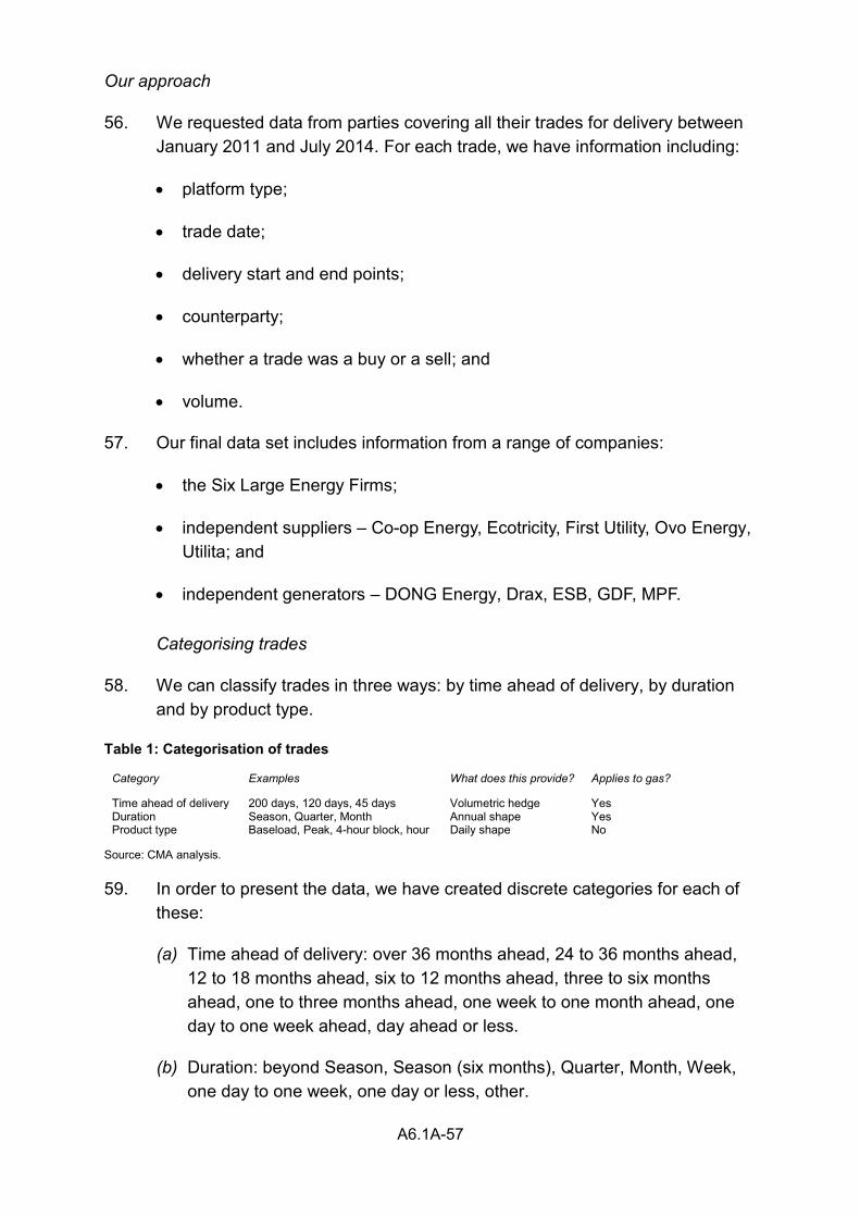
A6.1A-57

Our approach

56. We requested data from parties covering all their trades for delivery between

January 2011 and July 2014. For each trade, we have information including:

platform type;

trade date;

delivery start and end points;

counterparty;

whether a trade was a buy or a sell; and

volume.

57. Our final data set includes information from a range of companies:

the Six Large Energy Firms;

independent suppliers – Co-op Energy, Ecotricity, First Utility, Ovo Energy,

Utilita; and

independent generators – DONG Energy, Drax, ESB, GDF, MPF.

Categorising trades

58. We can classify trades in three ways: by time ahead of delivery, by duration

and by product type.

Table 1: Categorisation of trades

Category Examples What does this provide? Applies to gas?

Time ahead of delivery 200 days, 120 days, 45 days Volumetric hedge Yes Duration Season, Quarter, Month Annual shape Yes Product type Baseload, Peak, 4-hour block, hour Daily shape No

Source: CMA analysis.

59. In order to present the data, we have created discrete categories for each of

these:

(a) Time ahead of delivery: over 36 months ahead, 24 to 36 months ahead,

12 to 18 months ahead, six to 12 months ahead, three to six months

ahead, one to three months ahead, one week to one month ahead, one

day to one week ahead, day ahead or less.

(b) Duration: beyond Season, Season (six months), Quarter, Month, Week,

one day to one week, one day or less, other.

A6.1A-58

(c) Product type: Half-hour, Hour, Half block (2 hours), Block (4 hours), Two

blocks (8 hours), Peak, Extended peak, Off peak, Baseload, Custom,

Other.

60. These ways of classifying trades form the basis for the questions we want to

examine using this trading data. The first question relates to the overall

volume of trading at different times ahead of delivery, while the second and

third questions address different types of shaping.

Figure 2: Key questions for trading data

Source: CMA analysis.

Sleeve trading

61. In the OTC market, firms need a bilateral trading agreement in place in order

to trade directly with each other. If they do not have an agreement, they can

try to trade via a third company (which has agreements with both firms). The

third company buys electricity from one firm, and sells the same amount to the

other firm. In this case, the third company is said to be acting as a sleeve.

A6.1A-59

62. Where a firm is acting as a sleeve, we have removed those trades as far as

possible before analysing its data.26 This is because they do not represent the

firm buying and selling electricity for itself.27

Our analysis and results

63. This section summarises the results of our analysis, with an effort to focus on

the key evidence. First, we look at volumes traded over time (paragraphs 64–

69). Second, we look at products by duration (paragraphs 71–81). Third, we

look at products by type (paragraphs 84–91).

Analysis: all products by volume

Six Large Energy Firms

64. Looking at overall volumes, we see that the majority of trading by the Six

Large Energy Firms was within a year ahead of delivery. This pattern is

consistent between parties. [] trading was within a year from delivery, giving

it the largest proportion among the Six Large Energy Firms. [].

Figure 3: Volume of trading by time ahead of delivery (all products) by the Six Large Energy Firms

[]

Source: CMA analysis, parties’ data. Note that the time categories in the chart are not of equal lengths.

65. However, the volumes traded towards the far end of the curve can still be

significant. For example, Centrica traded nearly [] per year over three years

ahead. As an illustration, [] supplied [] in the last year for which we have

data. This means that Centrica trades over [] times the size of a mid-tier

supplier at the far end of the curve.

66. We can also compare the Six Large Energy Firms. In most of the timeframes,

the order of which firms trade most is similar to the order of the size of their

GB businesses.28 Scottish Power and Centrica have the smallest businesses,

26 We asked parties to identify sleeve trades. Not all of them were able to do so. However, for firms who were able to provide this information, sleeve trades represented a small proportion of their overall traded volumes. The figure was [] for SSE and [] for Centrica. RWE could provide this information only for sample months, but it was between [] in each case. This suggests that any sleeve trades remaining in our data should not have a material effect on the results. 27 A firm that acts as a sleeve is helping to facilitate a trade that might not otherwise have been possible, and therefore this is a practice that benefits liquidity. When considering the effect of sleeve trades on quantified measures of liquidity, it would be sensible to consider both halves of a sleeve trade as a single trade, and remove one half. We understand that this is the approach taken by price reporting agencies. 28 Size of firms approximated based on the average of the sum of volumes generated and supplied in each of 2011, 2012 and 2013. Calculated from the segmental statements, available through Segmental statements. (SSE

A6.1A-60

and these firms trade the least. On an overall basis, the total amount traded

by each firm is greater than the size of its businesses in GB. The firm with the

smallest ratio was EDF, which traded [] the size of its physical business.

RWE had the largest ratio – it traded 4.3 times the size of its physical

business.29

Independent suppliers

67. We now look at a set of independent suppliers (Co-op Energy, Ecotricity, First

Utility, Ovo Energy and Utilita). The graph below shows that these firms

traded [] more than a year before the start of delivery in the period we

examined. (The combined trading of these five firms beyond a year ahead

was [] per year. This is equivalent to only [] in Seasonal Baseload.)30

This is in contrast to the Six Large Energy Firms, which all carry out some

trading right along the curve. Independent suppliers therefore traded nearer to

delivery than the Six Large Energy Firms on this metric.

Figure 4: Volume of trading by time ahead of delivery (all products) by independent suppliers

[]

Source: CMA analysis, parties’ data.

68. First Utility’s trading pattern was unusual. However, we understand that First

Utility’s trading pattern from this period was not typical of its current trading

owing to the change of trading counterparty during the period of observation.

Under its agreement with the intermediary it was using at that time, it was able

to obtain [] products. These trades cover a long period, even though they

start to deliver soon after they are agreed. The volume-weighted average

duration of First Utility’s trades (in the data we collected) was []. So on the

metric we have used – time to start of delivery – First Utility does very little

trading far ahead; but if we looked at time to end of delivery, []. We

understand that since it has changed intermediary to Shell, First Utility trades

mainly [] wholesale products. It now trades [] up to [] forward.

Therefore in our assessment of trading we have considered what First Utility

told us about its normal trading behaviour as well as its actual

(unrepresentative) behaviour in the period for which we collected data.

figures based on its financial year starting in April.) EDF Energy average 130.7TWh; RWE average 85.1TWh; SSE average 82.7TWh; E.ON average 75.8TWh; Centrica average 65.8TWh; Scottish Power average 42.1TWh. 29 This involves dividing the annual average volume traded by the average size of its physical business (as calculated above). Full results in the main body of this appendix. 30 The standard clip size for forward products is 10 MW, and there are 4,380 hours in a season.

A6.1A-61

Independent generators

69. We have a mixed picture from the independent generators in our data. GDF

looks similar to the Six Large Energy Firms – it trades electricity up to 36

months ahead, but the majority (88%) of its trading is within a year from

delivery. []. Drax also traded electricity at the far end of the curve – it was

the only independent generator to trade any volume before 36 months out.

However, Drax was somewhat different from the Six Large Energy Firms in

that the timeframe in which it traded the highest volume was between 18 and

12 months ahead (rather than closer to delivery).

70. In contrast, MPF looks more similar to the independent suppliers. []. ESB

presented a similar pattern, [].

Figure 5: Volume of trading by time ahead of delivery (all products) by independent generators

[]

Source: CMA analysis, parties’ data.

Analysis: by product duration

71. We now look at the different lengths of products. These products can help

firms to contract ahead to match their annual shape.

Six Large Energy Firms

72. For the Six Large Energy Firms, there is little trading of Monthly Baseload

beyond three months ahead of delivery. [] traded only [] of its Monthly

Baseload beyond three months ahead – and the proportions were even

smaller for the other parties. While most parties traded some volume in this

product beyond year-ahead, the total volume (across all six firms) was small –

under []TWh per year. This suggests that these firms manage their annual

shape near to delivery.

Figure 6: Volume of trading by time ahead of delivery by the Six Large Energy Firms – Monthly Baseload

[]

Source: CMA analysis, parties’ data. Note: This and the following Baseload charts for the Six Large Energy Firms are all plotted on the same scale to facilitate comparisons.

73. There is slightly more trading of Quarterly Baseload three to six months

before delivery (compared to Monthly Baseload). The Six Large Energy Firms

each traded at least 21% of their Quarterly Baseload beyond three months

A6.1A-62

ahead.31 In contrast, the Six Large Energy Firms trade Seasonal Baseload

along the curve – each of them traded some volume up to [] months ahead.

The volumes traded in this product are also much higher. Each of the Six

Large Energy Firms traded at least three times as much in Seasonal

Baseload as in Monthly Baseload, and at least five times as much as in

Quarterly Baseload.32 As trading in Monthly and Quarterly products falls away,

most trading beyond a year ahead is in Seasonal Baseload.

Figure 7: Volume of trading by time ahead of delivery by the Six Large Energy Firms – Quarterly Baseload

[]

Source: CMA analysis, parties’ data.

Figure 8: Volume of trading by time ahead of delivery by the Six Large Energy Firms – Seasonal Baseload

[]

Source: CMA analysis, parties’ data.

74. There is a similar pattern for Peak33 – Seasonal products are traded much

further ahead than Monthly or Quarterly products. (For all firms, the time

category with the highest volume of Monthly Peak was between a week and a

month from delivery, whereas for Seasonal Peak it was between six and 12

months ahead.) For Monthly Peak products, the amount of activity beyond

three months ahead is very small. [] traded 0.08TWh per year, which was

the most of any party; this is equivalent to 35 trades per year.34

Figure 9: Volume of trading by time ahead of delivery by the Six Large Energy Firms – Monthly Peak

[]

Source: CMA analysis, parties’ data. Note: Smaller scale for Peak charts than Baseload charts.

Figure 10: Volume of trading by time ahead of delivery by the Six Large Energy Firms – Quarterly Peak

[]

Source: CMA analysis, parties’ data.

31 [] traded the smallest proportion beyond three months ahead. 32 In each case, [] was the firm with the lowest ratios: [] between Seasonal Baseload and Monthly Baseload, and [] between Seasonal Baseload and Quarterly Baseload. 33 A product that delivers a flat volume between 7am and 7pm on weekdays. 34 Based on a standard forward clip size of 10 MW, and a four-week month under the EFA calendar.

A6.1A-63

Figure 11: Volume of trading by time ahead of delivery by the Six Large Energy Firms – Seasonal Peak

[]

Source: CMA analysis, parties’ data.

Independent suppliers

75. Like the Six Large Energy Firms, most independent suppliers trade Monthly

Baseload largely within three months of delivery. [] trades a significant

amount in this product within a week ahead (relative to its trading in other

timescales). Two independent suppliers traded some volume in Monthly

Baseload between [] ahead of start of delivery. For both of these firms, this

was as far ahead as they traded any product.35

Figure 12: Volume of trading by time ahead of delivery by independent suppliers – Monthly Baseload

[]

Source: CMA analysis, parties’ data. Note: This and the following Baseload charts for independent suppliers are all plotted on the same scale to facilitate comparisons.

76. One independent supplier did not trade Quarterly Baseload at all. For the

other four independent suppliers, the timeframe with the largest volume of

trading in Quarterly Baseload was [].

Figure 13: Volume of trading by time ahead of delivery by independent suppliers – Quarterly Baseload

[]

Source: CMA analysis, parties’ data.

77. Ovo Energy traded its largest volume of Seasonal Baseload between six and

12 months from delivery. This is further ahead than it traded months and

quarters. [] also traded seasons further ahead than it traded months and

quarters. Each of the other three independent suppliers in this data traded the

equivalent of [] per year in Seasonal Baseload.36

Figure 14: Volume of trading by time ahead of delivery by independent suppliers – Seasonal Baseload

[]

Source: CMA analysis, parties’ data.

35 Over 99% of [] Baseload trading is in Months. 36 The results we calculated for First Utility may not be representative of its normal trading because of the way it traded in this period (discussed above).

A6.1A-64

78. Independent suppliers traded small volumes in Peak contracts. Only three

independent suppliers traded any Seasonal Peak, and only two firms traded

any Quarterly Peak.

79. For Monthly Peak, the graph below shows that independent suppliers fall into

two categories. Three independent suppliers traded all (or the vast majority of)

their Monthly Peak within three months from delivery. Two other independent

suppliers traded some Monthly Peak up to 12 or 18 months ahead, but even

these companies traded around half of their Monthly Peak within three months

of delivery.37

Figure 15: Volume of trading by time ahead of delivery by independent suppliers – Monthly Peak

[]

Source: CMA analysis, parties’ data. Note: Smaller scale for Peak chart than for Baseload.

Independent generators

80. Independent generators generally traded Baseload products of different

durations in a similar way to the Six Large Energy Firms (the exception was

[], which did not trade any Monthly, Quarterly or Seasonal Baseload

products):

(a) Independent generators mostly traded Monthly Baseload within [] of

delivery. The firm that traded the largest proportion beyond this was GDF

(13.1%).

(b) Independent generators generally traded Quarterly Baseload a little

further ahead than Monthly Baseload. Drax, [] and GDF all traded

around 40% of their Quarterly Baseload beyond three months from

delivery.

(c) [] independent generators traded some Seasonal Baseload at least two

years ahead. However, each of these firms traded at least half of its

Seasonal Baseload within a year from delivery.

Figure 16: Volume of trading by time ahead of duration by independent generators – Monthly Baseload

[]

Source: CMA analysis, parties’ data.

37 [] traded 48% of its Monthly Peak within three months of delivery. [] traded 51% of its Monthly Peak within three months of delivery.

A6.1A-65

Figure 17: Volume of trading by time ahead of duration by independent generators – Quarterly Baseload

[]

Source: CMA analysis, parties’ data.

Figure 18: Volume of trading by time ahead of duration by independent generators – Seasonal Baseload

[]

Source: CMA analysis, parties’ data.

81. Independent generators traded small volumes in Peak products. For example,

GDF traded the most Monthly Peak, but still traded 8.6 times as much volume

in Monthly Baseload. [], and []. [].

82. Subject to these caveats, the pattern of when independent generators traded

Peak products was similar to when they traded Baseload. For example, there

was little trading of Monthly Peak beyond three months ahead. GDF traded

9.3% of its Monthly Peak beyond this point, which was the most of any

independent generator.

Figure 19: Volume of trading by time ahead of duration by independent generators – Monthly Peak

[]

Source: CMA analysis, parties’ data.

Summary

83. The overall pattern (across all firm types) is therefore that Monthly products

were generally traded within three months of delivery. Quarterly products

were traded slightly further ahead, but this trading was nearly all within six

months of delivery. Seasonal products were traded the furthest out.

Analysis: by product type

84. We now look at products other than Baseload and Peak. For the Six Large

Energy Firms, the charts above (Figures 9, 10 and 11) show that most Peak

trading was within a year from delivery. Peak was the third most important

product type for the Six Large Energy Firms (after Baseload and individual

Hours), but it still represented only 4.3% of their total traded volumes. Even

within one year from delivery, Peak still made up less than 5% of total traded

volumes by the Six Large Energy Firms.

85. We also looked at a wider range of products. For electricity trading, the day is

divided into six Blocks of four hours. These are standardised – eg Block 5 is

3pm to 7pm. We created the category of ‘other standard products’, which

A6.1A-66

looks at four-hour Blocks, and cases where multiple Blocks are traded

together (eg Overnights). It does not include Peak, as this has been covered

separately.

Figure 20: Volume of trading by time ahead of delivery by the Six Large Energy Firms – other standard products

[]

Source: CMA analysis, parties’ data. Note: The product types included in this category are: four-hour Blocks, pairs of four-hour Blocks, Off-peak and Extended peak.

86. The graph above shows that there are differences between firms. Two parties

traded significantly more in these products than the other four parties in most

timeframes. For example, between three and six months ahead, RWE traded

an average of 2.0TWh per year and SSE traded [] per year; the other four

firms each traded under [] per year. However, all firms carried out at least

70% of their trading in these products within three months from delivery, and

the largest category for each party was day or less. This supports the

proposition that firms generally shape their positions close to delivery.

87. We looked at independent suppliers’ trading of Peak in paragraphs 78 and 79.

Overall, at least half of each firm’s trading in Peak occurred within three

months of delivery.

88. Independent suppliers also traded ‘other standard products’ mostly within []

from delivery.38 []. []. This perhaps illustrates that independent suppliers

find different ways to manage their shape.

Figure 21: Volume of trading by time ahead of delivery by independent suppliers – other standard products

[]

Source: CMA analysis, parties’ data. Note: The product types included in this category are: four-hour Blocks, pairs of four-hour Blocks, Off-peak and Extended peak.

89. For independent generators, we covered Peak trading in paragraphs 81 and

82. []. The exception was GDF, whose trading in Peak started to fall away

only beyond year-ahead.

90. Independent generators generally traded other standard products only within

a month from delivery. [] generally traded very limited volumes in these

products beyond a month.) Drax traded only small volumes beyond this point.

GDF’s trading in other standard products looks more similar to that of some of

the Six Large Energy Firms. It traded some volume in other standard products

38 The results we calculated for First Utility may be misleading because of the way it traded in this period (discussed above).

A6.1A-67

up to two years ahead, although it still traded three-quarters of its volume

within a month of delivery.

Figure 22: Volume of trading by time ahead of delivery by independent generators – other standard products

[]

Source: CMA analysis, parties’ data. Note: The product types included in this category are: four-hour Blocks, pairs of four-hour Blocks, Off-peak and Extended peak.

91. This section therefore shows that Peak is not traded as far out from delivery

as Baseload, and that more specialised products are traded in a similar or

shorter timeframe. The reason for this could be either a lack of demand for

non-Baseload products or limited product availability. Credit and collateral is a

less likely explanation, because we expect credit costs to be driven more by

the time ahead of delivery than by the product type.

Comparison with gas

92. In this section we perform similar analysis on the pattern of trading in gas. We

look first at all products by volume over time, and then at product duration.

There is no equivalent ‘product type’ in gas because it is a daily product rather

than half hourly, so there is no within-day shape.

Gas trading – all products by volume

93. The graph below shows gas trading by time ahead of delivery for the Six

Large Energy Firms. Overall, the Six Large Energy Firms carried out 85% of

their gas trading within a year from delivery, and that pattern was broadly

similar across all six firms.

Figure 23: Gas trading by time ahead of delivery – Six Large Energy Firms

[]

Source: CMA analysis, parties’ data.

94. The proportion of trading at the far end of the curve was small, although

volumes were still large. The Six Large Energy Firms traded only 4.3% of their

volumes beyond two years out. Three firms ([], [] and RWE) traded more

beyond two years ahead than the size of their gas supply business.39 (This

does not give a full picture of firms’ gas requirements, as they also need to

buy fuel for their gas-fired power stations.) This suggests that these firms are

39 Comparing the annual average volume traded between 2011 and July 2014 (from our data set), and the annual average volume supplied between 2011 and 2013 (from firms’ Segmental statements, which are available on the Ofgem website).

A6.1A-68

able to trade reasonable volumes far out from delivery, but prefer to

concentrate the bulk of their trading within year.

95. The pattern of the Six Large Energy Firms’ gas trading was also similar to

their electricity trading. The table below compares gas and electricity trading

for the Six Large Energy Firms. The overall distribution of trading between

times ahead of delivery appears similar to that for electricity. The biggest

difference is that [] trades a greater proportion of its gas within a year from

delivery, compared to electricity.

Table 2: Percentage of each firm’s traded volume by time ahead of delivery – comparison between electricity and gas

%

Time ahead

Centrica E.ON EDF Energy

Electricity Gas Electricity Gas Electricity Gas

Beyond 3 years [] [] [] [] [] [] 2 to 3 years [] [] [] [] [] [] 1 to 2 years [] [] [] [] [] [] Inside 1 year [] [] [] [] [] []

Time ahead

RWE Scottish Power SSE

Electricity Gas Electricity Gas Electricity Gas

Beyond 3 years [] [] [] [] [] [] 2 to 3 years [] [] [] [] [] [] 1 to 2 years [] [] [] [] [] [] Inside 1 year [] [] [] [] [] []

Source: CMA analysis, parties’ data.

96. For independent suppliers, most trading was also within a year from delivery.

92.3% of gas trading by these firms combined occurred in this timeframe. This

appears to be a similar result to their electricity trading. This might suggest

that they are not taking advantage of any greater product availability in gas.

Figure 24: Gas trading by time ahead of delivery – independent suppliers

[]

Source: CMA analysis, parties’ data.

97. First Utility’s trading was []. However, as with electricity, its trades delivered

over a long period.40 The average length of its trades was [] days.

Therefore, its trading is again difficult to compare with that of other firms. If we

omit First Utility from the calculation above, 75.4% of gas trading by the other

independent suppliers was within year.

40 The results we calculated for First Utility may be misleading as to First Utility’s normal trading behaviour because of the way it traded in this period (discussed above).

A6.1A-69

Gas trading – Monthly products

98. The graph below shows that the majority of trading in Monthly gas products by

the Six Large Energy Firms was within three months of delivery.41 This is in

line with the qualitative statements we received on the length of liquidity in

Monthly products. These suggested that liquidity was lower beyond four to six

months out.42

Figure 25: Gas trading in Monthly products – Six Large Energy Firms

[]

Source: CMA analysis, parties’ data.

99. If the Six Large Energy Firms were using internal transfers and/or an implicit

hedge to provide Monthly shape in electricity, then we might expect them to

trade Monthly products further out in gas. As this is not happening, there may

simply be a lack of demand for Monthly products beyond a certain point. Even

in the gas market, which is reputed to be liquid, trading of more granular

products is concentrated closer to delivery.

100. Most of the independent suppliers for which we have data seemed to trade

some Monthly products over six months ahead. This applies to []. All these

firms use an intermediary which provides them with access to Monthly

products.43 First Utility had a [].

Figure 26: Gas trading in Monthly products – independent suppliers

[]

Source: CMA analysis, parties’ data.

101. By itself, this does not say anything about the availability of Monthly products

in gas relative to electricity. [] do not have agreements with intermediaries

in electricity. It is possible that they could therefore obtain Monthly products

more easily in electricity if they had equivalent agreements; but it is also

plausible that this would be more expensive if these products were less

available.

Gas trading – Quarterly products

102. The pattern for Quarterly products was similar to that for electricity. For the

Six Large Energy Firms, the timeframe with the highest traded volumes was

41 The chart shows RWE trading Monthly products beyond this, but RWE told us that this is not correct. RWE informed us that ‘the exchange trades that are reported as Monthly also include trades that may be Quarterly, Seasonal or Annual (because of the way the exchange records transactions)’ 42 Beyond four Months according to First Utility and Scottish Power, five months according to RWE, and six months according to Co-op Energy. 43 [].

A6.1A-70

between one month and three months ahead. There was also some trading

up to a year ahead, and negligible volumes beyond this.

Figure 27: Gas trading in Quarterly products – Six Large Energy Firms

[]

Source: CMA analysis, parties’ data.

103. First Utility was the only independent supplier to trade large amounts of

Quarterly products. Over [] of its Quarterly gas trading was between [].

Figure 28: Gas trading in Quarterly products – independent suppliers

[]

Source: CMA analysis, parties’ data.

Gas trading – Seasonal products

104. As in electricity, the Six Large Energy Firms traded Seasonal products much

further along the curve than Monthly or Quarterly products. However, the

volumes traded within year were still the most significant. For each of the

parties, the three timeframes with the highest volumes were those between

one month and 12 months ahead.

Figure 29: Gas trading in Seasonal products – Six Large Energy Firms

[]

Source: CMA analysis, parties’ data.

105. Independent suppliers traded minimal amounts of Seasonal gas – []. None

of the trading that did occur was beyond [] ahead.44

Figure 30: Gas trading in Seasonal products – independent suppliers

[]

Source: CMA analysis, parties’ data.

Product availability, spreads and depth

106. We obtained data on ‘bids’ and ‘asks’ in the OTC market from the four brokers

active in the market in that period: GFI, ICAP, Marex Spectron and Tullett

Prebon. (Bids are the prices at which parties are willing to buy; asks

(sometimes known as offers) are the prices at which parties are willing to sell.)

This took the form of snapshot data for 8am, 11am and 4pm on the second

44 In the case of First Utility, this may be misleading because of the way it traded in this period (discussed above). First Utility told us that it now trades up to [] ahead [] (similar to its trading in electricity)

A6.1A-71

Tuesday of every month from January 2011 to October 2014.45 We asked

each broker for the best bids up to 50 MW in depth for each available product

in each snapshot, and the equivalent best asks.

107. We combined this data into a common database that therefore showed all the

best bids and asks in the market at those points in time. This would be

equivalent to what a trader could have seen on a Trayport screen at those

moments.46 We used this to calculate, for each product, the spread between

the best available bid price and the best available ask price. We also

calculated the spreads at various different depths. For example, if someone

wanted to buy 50 MW of a product, they would be interested in the weighted

average of the ask prices for the cheapest 50 MW available.

108. The results we present below focused on the 11am snapshot, noting that this

generally had the best product availability of our three times of day. As

appropriate, we also note changes in the data since Ofgem introduced its

S&P licence conditions, which are first reflected in our data in April 2014.

109. First, we show spreads (expressed as a percentage of the bid price) for

products that were available to both buy and sell in any quantity. In all of

these charts, months when products were available are marked with a dot,

and those dots are joined with lines to help identify trends.

110. Figure 31 shows Baseload Seasonal products, which tend to have the best

availability. Seasons+1, +2, +3 and +4 were available in almost every month

in the period and at relatively tight spreads, particularly later in the period.

Trading in these products would let a party purchase energy more than two

years in advance of delivery. By contrast, Season+7 was available on only

four of the days in our sample, and always at spreads of greater than 1.5%;

and Season+8 only twice (one instance not shown because the spread was

too wide for the axis we used).

45 We chose this day in the hope that it would be representative (eg generally free of bank holidays). We chose two times that fell within Ofgem’s designated S&P windows (10:30am to 11:30am and 3:30pm to 4:30pm) and one that did not. We understand that Ofgem selected windows to coincide with times of day when traders were relatively active in forward products. Indeed, our data suggested that there were consistently more products available to trade at 11am and 4pm than at 8am. 46 For products where more than 50 MW was available from one broker, we would not have the full set of possible trades, but we thought 50 MW was a reasonable cut-off (as 50 MW represents a substantial amount of electricity – for a Seasonal Baseload product, this could be worth around £10 million).

A6.1A-72

Figure 31: Spreads on Baseload Seasonal products

Source: CMA analysis, broker data. Note: Solid lines are products that are included in the S&P Market Making obligation (since 31 March 2014).

111. Figure 32 shows Baseload Quarterly products. Availability here was worse

and spreads were wider. Quarters beyond Quarter+4 were not available on

any day in our data set. Even for Quarter+1 the spread is very variable until

S&P comes into effect. The tight spreads on Quarter+1 – the only one to be

included in S&P – after that point do not seem to have encouraged availability

of subsequent Quarters.

-0.5%

0.0%

0.5%

1.0%

1.5%

2.0%

2.5%

3.0%

3.5%

4.0%

Jan-1

1

Ma

r-1

1

Ma

y-1

1

Jul-1

1

Sep-1

1

No

v-1

1

Jan-1

2

Ma

r-1

2

Ma

y-1

2

Jul-1

2

Sep-1

2

No

v-1

2

Jan-1

3

Ma

r-1

3

Ma

y-1

3

Jul-1

3

Sep-1

3

No

v-1

3

Jan-1

4

Ma

r-1

4

Ma

y-1

4

Jul-1

4

Sep-1

4

Season+1 Season+2 Season+3 Season+4

Season+5 Season+6 Season+7 Season+8

A6.1A-73

Figure 32: Spreads on Baseload Quarterly products

Source: CMA analysis, broker data. Note: Solid lines are products that are included in the S&P Market Making obligation (since 31 March 2014).

112. Figure 33 shows Baseload Monthly products. Availability here was better than

for Quarters, with sporadic availability up to Month+8 (only available on one

day in our sample). However, spreads are wider than for Seasonal products.

Only Month+1 has consistently low spreads until the introduction of S&P,

which covers Months +1 and +2. Again, there is no positive effect of S&P on

any other Monthly product; if anything, they look worse since April 2014.

0.0%

0.5%

1.0%

1.5%

2.0%

2.5%

3.0%

3.5%

4.0%

Jan-1

1

Ma

r-1

1

Ma

y-1

1

Jul-1

1

Sep-1

1

No

v-1

1

Jan-1

2

Ma

r-1

2

Ma

y-1

2

Jul-1

2

Sep-1

2

No

v-1

2

Jan-1

3

Ma

r-1

3

Ma

y-1

3

Jul-1

3

Sep-1

3

No

v-1

3

Jan-1

4

Ma

r-1

4

Ma

y-1

4

Jul-1

4

Sep-1

4

Quarter+1 Quarter+2 Quarter+3 Quarter+4

A6.1A-74

Figure 33: Spreads on Baseload Monthly products

Source: CMA analysis, broker data. Note: Solid lines are products that are included in the S&P Market Making obligation (since 31 March 2014).

113. The following three figures show the equivalent Peak products for Seasons,

Quarters and Months. Availability here was worse than for Baseload counter-

parts, but apart from that the patterns were similar. Seasons had good avail-

ability and spreads for Seasons+1 and +2, and at times as far as Season+4.

(The first three Seasons are covered in S&P.) Quarterly availability was poor

and spreads were wide until January 2014, when Quarter+1 spreads tight-

ened. (This product was included in S&P and its spread has remained at that

level since.) Months were somewhere in between, with S&P leading to more

consistent low spreads for the first two Months (which are the products

included in S&P).

0.0%

0.5%

1.0%

1.5%

2.0%

2.5%

3.0%

3.5%

4.0%

Jan-1

1

Ma

r-1

1

Ma

y-1

1

Jul-1

1

Sep-1

1

No

v-1

1

Jan-1

2

Ma

r-1

2

Ma

y-1

2

Jul-1

2

Sep-1

2

No

v-1

2

Jan-1

3

Ma

r-1

3

Ma

y-1

3

Jul-1

3

Sep-1

3

No

v-1

3

Jan-1

4

Ma

r-1

4

Ma

y-1

4

Jul-1

4

Sep-1

4

Month+1 Month+2 Month+3 Month+4

Month+5 Month+6 Month+7 Month+8

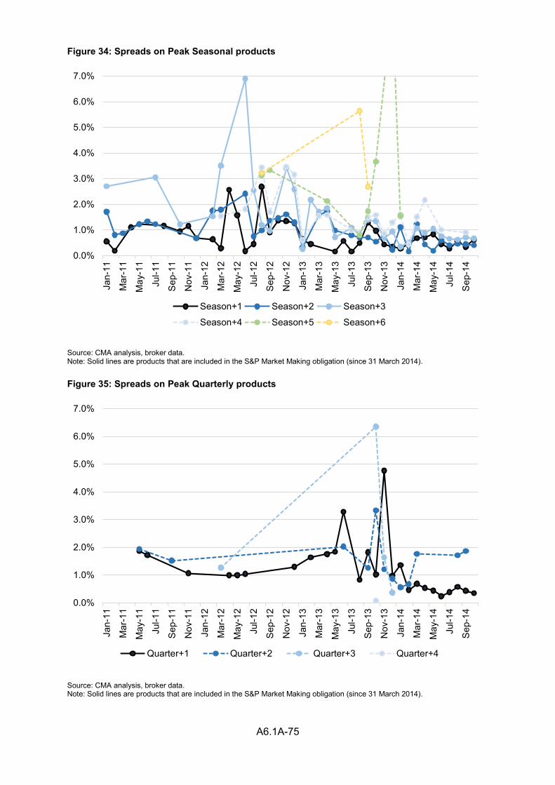
A6.1A-75

Figure 34: Spreads on Peak Seasonal products

Source: CMA analysis, broker data. Note: Solid lines are products that are included in the S&P Market Making obligation (since 31 March 2014).

Figure 35: Spreads on Peak Quarterly products

Source: CMA analysis, broker data. Note: Solid lines are products that are included in the S&P Market Making obligation (since 31 March 2014).

0.0%

1.0%

2.0%

3.0%

4.0%

5.0%

6.0%

7.0%

Jan-1

1

Ma

r-1

1

Ma

y-1

1

Jul-1

1

Sep-1

1

No

v-1

1

Jan-1

2

Ma

r-1

2

Ma

y-1

2

Jul-1

2

Sep-1

2

No

v-1

2

Jan-1

3

Ma

r-1

3

Ma

y-1

3

Jul-1

3

Sep-1

3

No

v-1

3

Jan-1

4

Ma

r-1

4

Ma

y-1

4

Jul-1

4

Sep-1

4

Season+1 Season+2 Season+3

Season+4 Season+5 Season+6

0.0%

1.0%

2.0%

3.0%

4.0%

5.0%

6.0%

7.0%

Jan-1

1

Ma

r-1

1

Ma

y-1

1

Jul-1

1

Sep-1

1

No

v-1

1

Jan-1

2

Ma

r-1

2

Ma

y-1

2

Jul-1

2

Sep-1

2

No

v-1

2

Jan-1

3

Ma

r-1

3

Ma

y-1

3

Jul-1

3

Sep-1

3

No

v-1

3

Jan-1

4

Ma

r-1

4

Ma

y-1

4

Jul-1

4

Sep-1

4

Quarter+1 Quarter+2 Quarter+3 Quarter+4

A6.1A-76

Figure 36: Spreads on Peak Monthly products

Source: CMA analysis, broker data. Note: Solid lines are products that are included in the S&P Market Making Obligation (since 31 March 2014).

114. In Table 3 below we summarise the availability information from the charts

above by showing the proportion of dates in our sample when each listed

product was available in any quantity to both buy and sell.47 Products covered

by the Market Making obligation in S&P are marked with an outline border.

Table 3: Proportion of days when product was available to both buy and sell (any quantity)

Time ahead of delivery (season, quarter, month, respectively)

+1 +2 +3 +4 +5 +6 +7 +8

Baseload Season 100% 100% 98% 93% 80% 54% 9% 4%

Quarter 85% 48% 30% 15% 0% 0% 0% 0%

Month 100% 98% 76% 59% 28% 15% 7% 2%

Peaks Season 85% 78% 70% 46% 17% 7% 0% 0%

Quarter 57% 26% 9% 2% 0% 0% 0% 0%

Month 93% 65% 46% 26% 17% 11% 7% 0%

Block 6 Month 33% 11% 0% 0% 2% 0% 0% 0%

Source: Data from brokers, CMA analysis. Note: Cells with borders are covered by Market Making Obligation in S&P.

115. This analysis suggested that availability of Baseload Season products was

very good for more than two years ahead of delivery. Peak Season products

47 In practice we found that it was rare for a product to be available to buy but not to sell, or vice versa.

0.0%

1.0%

2.0%

3.0%

4.0%

5.0%

6.0%

7.0%

Jan-1

1

Ma

r-1

1

Ma

y-1

1

Jul-1

1

Sep-1

1

No

v-1

1

Jan-1

2

Ma

r-1

2

Ma

y-1

2

Jul-1

2

Sep-1

2

No

v-1

2

Jan-1

3

Ma

r-1

3

Ma

y-1

3

Jul-1

3

Sep-1

3

No

v-1

3

Jan-1

4

Ma

r-1

4

Ma

y-1

4

Jul-1

4

Sep-1

4

Month+1 Month+2 Month+3 Month+4

Month+5 Month+6 Month+7

A6.1A-77

were not always available, but had reasonable availability (70% or more)

three seasons ahead. Baseload Months were almost always available two

months ahead, and Peak Month availability was best one month ahead.

Quarters were worse than Peaks.

116. Other products had relatively little availability. For example, one product that

we might expect to be attractive to domestic suppliers is Block 6, which runs

from 7pm to 11pm and so adds an evening shape to the standard Peak

product (7am to 7pm). We found that Block 6 products were rarely available to

both buy and sell – the most commonly traded was a Monthly product for the

month ahead, available on a third of the dates in our data set (see Table 3).

117. We also looked at spreads. We looked at how often a product had a spread of

1% or less,48 and the pattern was broadly similar to that in Table 3, above, but

with smaller numbers. There were only nine products with a spread this tight

in at least half of the days in our sample: for Baseload, the first four Seasons,

one Quarter and two Months; and for Peak, the first Season and Month. In our

entire sample there are only three occurrences of a Block 6 product with a

spread that tight: a Monthly product on two days, and a Quarterly product on

one day.

Table 4: Proportion of days when product was available with a spread of no more than 1% (any depth)

%

Time ahead of delivery (season, quarter, month, respectively)

+1 +2 +3 +4 +5 +6 +7 +8

Baseload Season 100 89 78 61 35 7 0 0

Quarter 59 15 7 7 0 0 0 0

Month 98 76 28 13 4 4 0 0

Peaks Season 61 46 30 11 2 0 0 0

Quarter 28 7 2 2 0 0 0 0

Month 72 26 7 4 0 0 0 0

Block 6 Month 4 0 0 0 0 0 0 0

Source: Data from brokers, CMA analysis. Note: Cells with borders are covered by Market Making Obligation in S&P.

118. We also looked at data at 8am, outside the windows. Figure 37 shows

spreads for Baseload Seasonal products (the most liquid products). This can

be compared with Figure 31, which shows the same products at 11am.

Availability and spreads are noticeably worse at 8am, and this was also true

of the other products we reviewed. We also notice that spreads at 8am

appear to have become worse following the introduction of S&P.

48 1% is the largest of the permitted spreads under the S&P Market Making obligation.

A6.1A-78

Figure 37: Spreads on Baseload Seasonal products (any depth), 8am

Source: CMA analysis, broker data. Note: Solid lines are products that are included in the S&P Market Making Obligation (since 31 March 2014).

Depth

119. We considered how the results in the previous section varied when we

increased product depth. A common clip size is 10 MW, and at that depth we

generally found that the same range of products was available. However, if

we increased the clip size to 50 MW, availability declined substantially. Table

5 shows that at this clip size it would not be possible to guarantee that any

product would be available to buy and sell at 11am on any given day (prior to

S&P). Only Season+1 and Month+1 Baseload products looked to have

reasonable availability over the period of our sample. Those products covered

by the Market Making obligation under S&P have been available at this depth

since it came into effect, and will continue to be as long as the obligation is in

effect. This means that many of the products here effectively have long

periods of little or no availability before that time, followed by constant

availability since then. This can be seen in the charts below.

0.0%

0.5%

1.0%

1.5%

2.0%

2.5%

3.0%

3.5%

4.0%

Jan-1

1

Ma

r-1

1

Ma

y-1

1

Jul-1

1

Sep-1

1

No

v-1

1

Jan-1

2

Ma

r-1

2

Ma

y-1

2

Jul-1

2

Sep-1

2

No

v-1

2

Jan-1

3

Ma

r-1

3

Ma

y-1

3

Jul-1

3

Sep-1

3

No

v-1

3

Jan-1

4

Ma

r-1

4

Ma

y-1

4

Jul-1

4

Sep-1

4

Season+1 Season+2 Season+3 Season+4

Season+5 Season+6 Season+7 Season+8

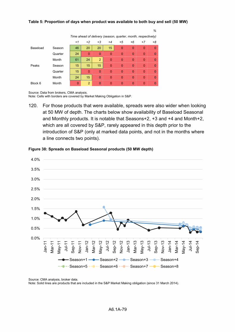
A6.1A-79

Table 5: Proportion of days when product was available to both buy and sell (50 MW)

%

Time ahead of delivery (season, quarter, month, respectively)

+1 +2 +3 +4 +5 +6 +7 +8

Baseload Season 46 20 20 15 0 0 0 0

Quarter 24 0 0 0 0 0 0 0

Month 61 24 2 0 0 0 0 0

Peaks Season 15 15 15 0 0 0 0 0

Quarter 15 0 0 0 0 0 0 0

Month 24 15 0 0 0 0 0 0

Block 6 Month 0 2 0 0 0 0 0 0

Source: Data from brokers, CMA analysis. Note: Cells with borders are covered by Market Making Obligation in S&P.

120. For those products that were available, spreads were also wider when looking

at 50 MW of depth. The charts below show availability of Baseload Seasonal

and Monthly products. It is notable that Seasons+2, +3 and +4 and Month+2,

which are all covered by S&P, rarely appeared in this depth prior to the

introduction of S&P (only at marked data points, and not in the months where

a line connects two points).

Figure 38: Spreads on Baseload Seasonal products (50 MW depth)

Source: CMA analysis, broker data. Note: Solid lines are products that are included in the S&P Market Making obligation (since 31 March 2014).

0.0%

0.5%

1.0%

1.5%

2.0%

2.5%

3.0%

3.5%

4.0%

Jan-1

1

Ma

r-1

1

Ma

y-1

1

Jul-1

1

Sep-1

1

No

v-1

1

Jan-1

2

Ma

r-1

2

Ma

y-1

2

Jul-1

2

Sep-1

2

No

v-1

2

Jan-1

3

Ma

r-1

3

Ma

y-1

3

Jul-1

3

Sep-1

3

No

v-1

3

Jan-1

4

Ma

r-1

4

Ma

y-1

4

Jul-1

4

Sep-1

4

Season+1 Season+2 Season+3 Season+4

Season+5 Season+6 Season+7 Season+8

A6.1A-80

Figure 39: Spreads on Baseload Monthly products (50 MW depth)

Source: CMA analysis, broker data. Note: Solid lines are products that are included in the S&P Market Making obligation (since 31 March 2014).

Active players

121. We looked at the whole data set to see who was involved in placing orders to

trade, and who was offering the best prices for each product. We found that

just over 70% of both bids and asks were from the Six Large Energy Firms.

We also found that more than two-thirds of best prices are from the Six Large

Energy Firms (ie roughly in proportion to the number of orders to trade).

Table 6: Proportion of orders to trade by the Six Large Energy Firms

%

All futures

Baseload and Peak

products

Bids Asks Bids Asks

Percentage of prices posted by SLEFs 70.6 71.4 72.9 70.9

Percentage of best prices posted by

SLEFs 67.4 70.1 69.4 67.1

Source: CMA analysis, broker data.

0.0%

0.5%

1.0%

1.5%

2.0%

2.5%

3.0%

3.5%

4.0%

Jan-1

1

Ma

r-1

1

Ma

y-1

1

Jul-1

1

Sep-1

1

No

v-1

1

Jan-1

2

Ma

r-1

2

Ma

y-1

2

Jul-1

2

Sep-1

2

No

v-1

2

Jan-1

3

Ma

r-1

3

Ma

y-1

3

Jul-1

3

Sep-1

3

No

v-1

3

Jan-1

4

Ma

r-1

4

Ma

y-1

4

Jul-1

4

Sep-1

4

Month+1 Month+2 Month+3 Month+4

Month+5 Month+6 Month+7 Month+8

A6.1A-81

Market close data

Electricity

122. We also looked at data from ICIS Heren, which provided daily data on

assessed product spreads at market close from January 2010.49 The market

close here is at the end of the afternoon S&P window, hence this data is likely

to reflect availability during that window and does not tell us about other times

of day outside the windows. The following four charts show monthly averages

of this daily data for key Baseload and Peak products. We can make the

following observations:

(a) Spreads get wider further from delivery.

(b) Seasons have tighter spreads than Months, which in turn are tighter than

Quarters.

(c) Baseload has tighter spreads than Peak.

(d) the introduction of S&P, seen in this data since April 2014, has led to

tighter spreads in mandated products, but there has been no apparent

positive effect on other products. (For example, Season+3 and Season+4

Peak generally had similar spreads prior to the introduction of S&P.

Season+3 Peak is a mandated product, and so the spreads have fallen

since, but spreads for Season+4 Peak have increased.)

49 ICIS Heren’s assessments are ‘based on bids and offers widely available to the market closest to the typically observed last point of liquidity’, which for GB is 4.30pm (apart from Day Ahead and Weekend products, which we excluded from this analysis). Where a bid or offer is not available, ICIS Heren ‘will work back in time from its published closing time to the last point of liquidity during the trading session and assess value at that point’, according to its published methodology. See ICIS Heren (2014) European daily electricity markets methodology.

This does not account for product depth.

A6.1A-82

Figure 40: Monthly average spreads for Seasonal Baseload products

Source: CMA analysis, ICIS Heren data. Note: Solid lines are products that are included in the S&P Market Making obligation (since 31 March 2014).

Figure 41: Monthly average spreads for Quarterly and Monthly Baseload products

Source: CMA analysis, ICIS Heren data. Note: Solid lines are products that are included in the S&P Market Making obligation (since 31 March 2014).

0.0%

0.5%

1.0%

1.5%

2.0%

2.5%

Jan-1

0

Apr-

10

Jul-1

0

Oct-

10

Jan-1

1

Apr-

11

Jul-1

1

Oct-

11

Jan-1

2

Apr-

12

Jul-1

2

Oct-

12

Jan-1

3

Apr-

13

Jul-1

3

Oct-

13

Jan-1

4

Apr-

14

Jul-1

4

Oct-

14

Season+1

Season+2

Season+3

Season+4

Season+5

Season+6

Season+7

0.0%

0.5%

1.0%

1.5%

2.0%

2.5%

3.0%

Jan-1

0

Apr-

10

Jul-1

0

Oct-

10

Jan-1

1

Apr-

11

Jul-1

1

Oct-

11

Jan-1

2

Apr-

12

Jul-1

2

Oct-

12

Jan-1

3

Apr-

13

Jul-1

3

Oct-

13

Jan-1

4

Apr-

14

Jul-1

4

Oct-

14

Month+1

Month+2

Month+3

Month+4

Quarter+1

Quarter+2

Quarter+3

Quarter+4

A6.1A-83

Figure 42: Monthly average spreads for Seasonal Peak products

Source: CMA analysis, ICIS Heren data. Note: Solid lines are products that are included in the S&P Market Making obligation (since 31 March 2014).

Figure 43: Monthly average spreads for Quarterly and Monthly Peak products

Source: CMA analysis, ICIS Heren data. Note: Solid lines are products that are included in the S&P Market Making obligation (since 31 March 2014).

0.0%

0.5%

1.0%

1.5%

2.0%

2.5%

Jan-1

0

Apr-

10

Jul-1

0

Oct-

10

Jan-1

1

Apr-

11

Jul-1

1

Oct-

11

Jan-1

2

Apr-

12

Jul-1

2

Oct-

12

Jan-1

3

Apr-

13

Jul-1

3

Oct-

13

Jan-1

4

Apr-

14

Jul-1

4

Oct-

14

Season+1

Season+2

Season+3

Season+4

Season+5

Season+6

Season+7

0.0%

0.5%

1.0%

1.5%

2.0%

2.5%

3.0%

Jan-1

0

Apr-

10

Jul-1

0

Oct-

10

Jan-1

1

Apr-

11

Jul-1

1

Oct-

11

Jan-1

2

Apr-

12

Jul-1

2

Oct-

12

Jan-1

3

Apr-

13

Jul-1

3

Oct-

13

Jan-1

4

Apr-

14

Jul-1

4

Oct-

14

Month+1

Month+2

Month+3

Month+4

Quarter+1

Quarter+2

Quarter+3

Quarter+4

A6.1A-84

Gas

123. Gas products had tighter spreads than their electricity equivalents. There was

also a larger number of products within a given spread – for example, the

chart below shows eight Seasonal gas products with a spread of under 1%,

compared to generally four or five Seasonal Baseload products for electricity.

The main divergence in the pattern among products was that, for gas, Monthly

spreads were tighter than equivalent Seasonal spreads.

Figure 44: Monthly average spreads for seasonal gas products

Source: CMA analysis, ICIS Heren data.

0.0%

0.2%

0.4%

0.6%

0.8%

1.0%

1.2%

01

/01

/201

1

01

/03

/201

1

01

/05

/201

1

01

/07

/201

1

01

/09

/201

1

01

/11

/201

1

01

/01

/201

2

01

/03

/201

2

01

/05

/201

2

01

/07

/201

2

01

/09

/201

2

01

/11

/201

2

01

/01

/201

3

01

/03

/201

3

01

/05

/201

3

01

/07

/201

3

01

/09

/201

3

01

/11

/201

3

01

/01

/201

4

01

/03

/201

4

01

/05

/201

4

01

/07

/201

4

01

/09

/201

4

01

/11

/201

4

Season+1

Season+2

Season+3

Season+4

Season+5

Season+6

Season+7

Season+8

A6.1A-85

Figure 45: Monthly average spreads for Quarterly and Monthly gas products

Source: CMA analysis, ICIS Heren data.

124. ICIS Heren also recorded when its spread data was based on actual bids and

offers in the market at their designated market close time, and when it had to

default to other market data; this distinction could be used as an indicator of

availability. Table 7 shows the results of our analysis of this. It suggests that

availability is better for Baseload than Peak, better for Seasons than for

Months than for Quarters, and better close to delivery – all of which is

consistent with our other analysis. The same pattern is true of gas. We note

that the figures for electricity cannot be compared with those for gas: ICIS

Heren told us that because gas is more liquid than electricity, the standards

for bid-offer confirmation are higher.

0.0%

0.1%

0.2%

0.3%

0.4%

0.5%

0.6%

01

/01

/201

1

01

/03

/201

1

01

/05

/201

1

01

/07

/201

1

01

/09

/201

1

01

/11

/201

1

01

/01

/201

2

01

/03

/201

2

01

/05

/201

2

01

/07

/201

2

01

/09

/201

2

01

/11

/201

2

01

/01

/201

3

01

/03

/201

3

01

/05

/201

3

01

/07

/201

3

01

/09

/201

3

01

/11

/201

3

01

/01

/201

4

01

/03

/201

4

01

/05

/201

4

01

/07

/201

4

01

/09

/201

4

01

/11

/201

4

Month+1

Month+2

Month+3

Month+4

Quarter+1

Quarter+2

Quarter+3

Quarter+4

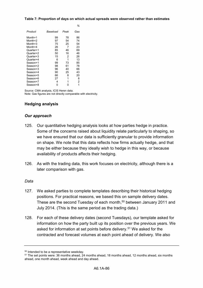
A6.1A-86

Table 7: Proportion of days on which actual spreads were observed rather than estimates

%

Product Baseload Peak Gas

Month+1 99 78 86 Month+2 97 54 74 Month+3 75 25 54 Month+4 26 7 23 Quarter+1 85 46 69 Quarter+2 50 16 46 Quarter+3 15 2 26 Quarter+4 6 1 13 Season+1 99 73 85 Season+2 98 61 78 Season+3 96 40 66 Season+4 90 25 43 Season+5 66 8 20 Season+6 27 1 8 Season+7 4 1 2 Season+8 0 0 1

Source: CMA analysis, ICIS Heren data. Note: Gas figures are not directly comparable with electricity.

Hedging analysis

Our approach

125. Our quantitative hedging analysis looks at how parties hedge in practice.

Some of the concerns raised about liquidity relate particularly to shaping, so

we have ensured that our data is sufficiently granular to provide information

on shape. We note that this data reflects how firms actually hedge, and that

may be either because they ideally wish to hedge in this way, or because

availability of products affects their hedging.

126. As with the trading data, this work focuses on electricity, although there is a

later comparison with gas.

Data

127. We asked parties to complete templates describing their historical hedging

positions. For practical reasons, we based this on sample delivery dates.

These are the second Tuesday of each month,50 between January 2011 and

July 2014. (This is the same period as the trading data.)

128. For each of these delivery dates (second Tuesdays), our template asked for

information on how the party built up its position over the previous years. We

asked for information at set points before delivery.51 We asked for the

contracted and forecast volumes at each point ahead of delivery. We also

50 Intended to be a representative weekday. 51 The set points were: 36 months ahead, 24 months ahead, 18 months ahead, 12 months ahead, six months ahead, one month ahead, week ahead and day ahead.

A6.1A-87

asked for each firm’s contracted volume and final output or demand at

delivery.

129. As noted above, we want to understand whether there are issues about

hedging shape. This means that we asked parties to provide the information

above on a settlement period (half-hourly) basis.

130. We sent this questionnaire to the Six Large Energy Firms and to independent

suppliers and generators. We asked these parties to complete separate

templates for different business areas.52 The number of templates completed

by each party depended on:

(a) the scope of its activities – some parties do not participate in all business

areas;

(b) the categories it uses to manage its hedging;53 and

(c) the extent to which data was available.

131. The responses received are mostly complete. SSE was unable to fill out our

templates, because [].Some independent firms were unable to complete

the templates, though they did send us qualitative information. Some other

independent firms were unable to provide forecast volumes, or provided

forecasts for usage of their existing customers but not a forecast of the set of

customers they would have at the relevant point in the future, but were able to

provide contracted and final volumes.

52 For example, gas generation or domestic variable supply. 53 [].

A6.1A-88

Table 8: Electricity hedging templates completed by each party (at most disaggregated level)*

Party Generation Supply

Centrica Gas; Nuclear; Renewables Domestic variable; Domestic fixed; Non-domestic fixed

EDF Energy [] []

E.ON Coal; Gas; Renewables; Unallocated []

RWE Coal; Gas; Biomass; Oil; Lynemouth coal; Renewables; Cogeneration; Prompt embedded

Domestic; SME; I&C; Retail-generation netting

Scottish Power All All

Co-op Energy Domestic variable; Domestic fixed

First Utility All

Opus Microbusiness; I&C

Utilita All

Drax Coal

ESB Gas

GDF Rugeley; Saltend; Deeside; First Hydro

Intergen Gas

MPF Baglan Bay; Sutton Bridge; Severn

Source: Parties’ responses. *Some parties also provided summary templates at more aggregated levels.

Key measures

132. As with trading, we are interested in three areas:

(a) overall volumetric hedging;

(b) hedging of annual shape; and

(c) hedging of daily shape.

133. For overall volumetric hedging, we look at this on a percentage basis. Ideally

we would look at contracted volumes as a percentage of forecast volumes.54

However, as several independent firms were unable to provide forecast

volumes, we instead use final volumes.55 (See paragraph 136 for further

discussion of this.) We also note that this gives us an aggregate picture when

we look at an entire supply portfolio, but firms may hedge customers on fixed

54 The forecast volume represents the information available to a firm at the time it made its hedging decision. It is therefore reasonable to suppose that a firm’s hedging decisions are made in relation to this. The final volume may differ from the forecast volume for a variety of reasons, such as growth, changes in plant profitability, or deviations from seasonal normal weather. Another potential comparator would be contemporary actual demand. However, the construction of our data set means that we do not have information on this for all timeframes before the start of our delivery dates. 55 We present results on the same basis for all firms to aid comparability.

A6.1A-89

term contracts different from customers on variable contracts. For example,

we understand that some suppliers, for some types of customer, may hedge

‘back to back’, ie when a customer signed a fixed-term fixed-price contract,

the supplier buys the expected volume of that customer’s demand over the

whole term of the contract.56

134. It is possible for the contracted volume to be greater than the final volume,

meaning that the hedged percentage exceeds 100%. Suppliers sometimes

buy more than they need for a period and sell back to the market later (or vice

versa for generators). For example, this can happen at times of day with low

demand (eg overnight), if a firm is hedging by buying Baseload products

(which deliver the same volume throughout the day).

135. In order to summarise the volumetric hedge, we use the median hedged

percentage to compare firms. This reduces the impact of outliers on the

results, compared to using the mean. However, there can still be a large

degree of variability around the median. For example, the chart below

illustrates the overall supply hedge for []. The interquartile range is up to 24

percentage points, and the range between the 95th percentile and the 5th

percentile reaches a maximum of 70 percentage points.57

Figure 46: Example of hedge variability – contracted volume as a percentage of final demand for [] whole supply business

[]

Source: CMA analysis, party’s data. Note: 36m – 36 months ahead of delivery; 24m – 24 months ahead of delivery; 18m – 18 months ahead of delivery; 12m – 12 months ahead of delivery; 6m – six months ahead of delivery; 1m – one month ahead of delivery; wa – one week ahead of delivery; da – one day ahead of delivery; del – at delivery.

136. As noted above, our results use contracted volumes as a percentage of final

output or demand. However, for the Six Large Energy Firms, we also have

information about forecast output or demand. We can therefore compare

contracted volumes as a percentage of final volume, and contracted volumes

as a percentage of forecast volume. This allows us to see if there are any key

differences between two measures. The table below shows the percentage

56 This means that a portfolio of fixed-term customers, for a firm that was growing, would appear to be less than 100% hedged down the curve on our measure, even though it would consider itself to be fully hedged at any point in time. This was not a substantial issue for the Six Large Energy Firms since their customer volumes were generally not changing rapidly (in percentage terms) over this period. In any cases where we thought this may be an issue, we took it into consideration in interpreting the results. 57 To some extent, this variability may be the result of firms deliberately applying flexibility. For example, an internal document from GDF showed proposed upper and lower bounds for hedging, with around 30 percentage points difference.

A6.1A-90

point difference between the median hedge percentages using the two

metrics.58 It covers the Six Large Energy Firms’ supply businesses.

Table 9: Percentage point difference: median contracted volume as a percentage of final demand, minus median contracted volume as a percentage of forecast demand (based on the supply businesses of the Six Large Energy Firms)

Percentage point

Time ahead of delivery Centrica E.ON EDF Energy

RWE Scottish Power

[] [] [] [] [] [] [] [] [] [] [] [] [] [] [] [] [] [] [] [] [] [] [] [] [] [] [] [] [] [] [] [] [] [] [] [] [] [] [] [] [] [] [] [] [] [] [] [] [] [] [] [] [] []

Source: CMA analysis, parties’ data. Note: 36m – 36 months ahead of delivery; 24m – 24 months ahead of delivery; 18m – 18 months ahead of delivery; 12m – 12 months ahead of delivery; 6m – six months ahead of delivery; 1m – one month ahead of delivery; wa – one week ahead of delivery; da – one day ahead of delivery; del – at delivery.

137. The differences vary between firms: all of Scottish Power’s differences are

under [] percentage points, whereas E.ON’s largest difference is []

percentage points. The largest differences belong to three parties where the

percentage based on final demand is consistently smaller than the percentage

based on forecast demand. (This implies that the final demand is larger than

the forecast demand). In each case, we believe that these are due to parties’

forecast volumes not including parts of I&C demand. We believe that this

issue means our preferred approach is reasonable (especially when we look

at hedges that do not include I&C supply).59,60 We therefore proceed with

using the percentage based on final demand, while accepting that this may

have an effect on the hedged percentages of particular firms. (If anything,

using final volumes will underplay the extent to which these three parties are

hedged.)

138. For shaping, we present information on firms’ hedges graphically. To make it

easier to identify patterns in the graphs, we use the median contracted

volume as our metric.

58 This comparison is based on an identical set of observations for each metric. (We dropped any observations where final or forecast volumes were missing.) In the main body of the analysis, we have used only final volumes, and so we have not dropped observations where forecast volumes were missing. 59 []. 60 The two approaches would diverge more if a firm’s volume of customers diverged significantly from forecast in percentage terms (eg unexpectedly fast growth).

A6.1A-91

Supply hedging

Volumetric supply hedging – Six Large Energy Firms

139. The graph below shows the overall supply hedges for five of the Six Large

Energy Firms, based on their entire supply businesses.61

Figure 47: Median contracted volume as a percentage of final demand – Six Large Energy Firms – all supply

[]

Source: CMA analysis, parties’ data.

140. The graph shows that all of the Six Large Energy Firms have forward hedges

for their supply businesses which extend at least two years ahead. This is

aligned with the qualitative information we received from them.62 [] hedged

[] of its supply volumes 24 months out, making it the firm with the largest

median hedge at this point. There is a fairly similar pattern between these

firms, especially within 18 months from delivery. This might suggest that they

have a similar ability to hedge.

Volumetric supply hedging – comparing the Six Large Energy Firms and

independent suppliers

141. The graph below takes the previous graph and adds hedging profiles for

independent suppliers.

Figure 48: Median contracted volume as a percentage of final demand – Six Large Energy Firms and independent suppliers – all supply

[]

Source: CMA analysis, parties’ data.

142. Independent suppliers generally have shorter hedges than the Six Large

Energy Firms. Before a year ahead, all independent suppliers in our data

have smaller hedged percentages than the Six Large Energy Firms. Co-op

Energy, [] and Opus all carry out the bulk of their hedging [].63

143. The impression that independent suppliers have shorter hedges is also

confirmed by qualitative responses from independent suppliers:

61 As noted above, SSE was unable to provide data in the same format as other firms. 62 []. 63 In the case of First Utility, we calculated results that may be misleading as to its normal behaviour because of the way it traded in this period (discussed above). In addition, [].

A6.1A-92

(a) BES Utilities (BES) said that it traded only up to six to nine months ahead.

(b) Ecotricity said that its hedging strategy covered up to a year ahead.

(c) Ovo Energy provided information showing that its hedging extended

around 18 months into the future.64

(d) Spark said that its hedging strategy covered 18 months ahead, and that it

aimed to be fully hedged three to six months before delivery.

144. Despite this, the independent suppliers have similar hedged percentages to

the Six Large Energy Firms at the month-ahead stage. This suggests that

there is not a barrier to them achieving a volumetric hedge in this timeframe.

145. Independent suppliers have grown over the period. This means that the

forecast demand of an independent supplier in forward timeframes may

generally be smaller than its final demand. It is therefore possible that the

percentage based on final demand may underestimate the extent to which

growing independent suppliers were hedged. For example, Co-op Energy told

us that []. Our graph may therefore present an upper bound on the

difference in hedged percentages between the Six Large Energy Firms and

independent suppliers.

146. We also compared the hedged profiles of the Six Large Energy Firms and

independent suppliers in domestic supply. Independents also had shorter

hedges than the Six Large Energy Firms in this area. For example, [].

Independent suppliers ([]) had [].65

147. On its own, the picture of the Six Large Energy Firms hedging further out than

independent suppliers has a number of potential interpretations. These could

include liquidity, access to credit, or commercial choice. We therefore need to

look at this in the context of other information. However, Figure 48 might

suggest that the Six Large Energy Firms are not relying on the implicit hedge

between their generation and supply arms; if they were, we would expect to

see them having shorter hedges than independent suppliers.66

64 For example, Ovo Energy provided an internal document as part of its response to the trading questionnaire showing its hedged position for electricity in September 2014. At this stage, its longest hedge was until March 2016. 65 In the case of First Utility, the results we calculated may be misleading because of the way it traded in this period (discussed above). See also footnote 63, which also applies here. 66 As discussed in the main body of this appendix.

A6.1A-93

Annual shape

148. We looked at hedging for individual months in order to see whether firms’

contracted volumes reflect the relative demand in each month. In forward

timescales, this would be the case if firms were hedging using individual

Monthly products, but would not be true if firms were hedging using Seasonal

products (which deliver the same volume over six months).

The Six Large Energy Firms

149. The chart below shows contracted volumes for [] supply business. At six,

12, 18 and 24 months ahead, [] hedged volume increases over the summer

Season.67 In contrast, final consumption is lowest in July and August.68 This

appears to suggest that [] is using Seasonal products further ahead, and

leaving its Monthly trading nearer to delivery.

Figure 49: Median contracted volume (per settlement period) by month in summer – [] supply

[]

Source: CMA analysis, party’s data.

150. This picture is reasonably representative of the Six Large Energy Firms.

Paragraph 213 below provides more information on others of these firms, in

the context of comparing parties’ hedging and trading data.

Independent suppliers

151. For independent suppliers, there is a mixed picture. The graph below shows

the hedged position by month for Opus. Looking at 12 months and six months

ahead, the contracted volume increases over the summer Season. We

obtained a similar result for [].

67 This occurs because Seasonal products start in specific months, and because we would expect the volume of trading in a product to increase over time. We would therefore expect to see a greater volume hedged for months towards the end of a season (eg September) than at the start (eg April). To give a specific example, we think about Summer 2015 and look at each month from 12 months ahead. We assume that in April 2014 a firm has bought 50 MW of Summer 2015 product. It will continue to buy Summer 2015 over the following months – in each month, it might buy an extra 10 MW. By September 2014, the volume hedged for September 2015 will be 100 MW. By September 2014, it will also have hedged 100 MW for April 2015 – but our 12 month ahead chart looks at April 2015 only from the perspective of April 2014, not September 2014. So when the firm buys a Summer product, our 12 month ahead line slopes up. In contrast, if it were hedging using Monthly products, we would expect our 12 month ahead line to match the monthly shape of demand. Even if demand were flat across the summer, our 12 month ahead line would be flat. 68 This is indicated by the shape of [] contracted volume at delivery.

A6.1A-94

Figure 50: Median contracted volume (per settlement period) by month in summer – [] supply

[]

Source: CMA analysis, party’s data.

152. However, [] contracted volumes 12 months and six months ahead show

some signs of shaping by month. [].69

Figure 51: Median contracted volume (per settlement period) by month in summer – [] supply

[]

Source: CMA analysis, party’s data.

Daily shape

The Six Large Energy Firms

153. We are interested in when suppliers shape their contracted positions to reflect

the profile of their final demand over a day. First Utility suggested that the Six

Large Energy Firms could do this through internal trading, stating that ‘On a

forward basis, VI generators could sell bespoke forward shaped products to

their VI supply businesses.’ If this were the case, we would expect to see

each of the Six Large Energy Firms having a forward contracted profile that

follows the shape of its demand.

154. The evidence suggests that this is not the case. Most of the Six Large Energy

Firms seem to leave their shape trading to the near term,70 as illustrated by

the graph below for []. This graph shows [] median contracted position for

each settlement period, with each line representing a different time ahead of

delivery. The flat lines on the graph until the week-ahead stage indicate that

[] was trading only standard products, rather than a shape which looks like

its final demand. The main product used appears to be Baseload (flat lines

over the entire day), as well as small amounts of Peak (settlement periods

15–38). This is aligned with firms’ qualitative responses – [] provided

examples of their supply business placing orders for specific standard

products with their trading business.

Figure 52: Median contracted volume by settlement period – [] supply

[]

Source: CMA analysis, party’s data.

69 See footnote 35 above. 70 This is based on graphs similar to the one below for [].[]also told us it generally starts to trade shape two to three months before delivery.

A6.1A-95

155. One of the Six Large Energy Firms displays a different pattern to the rest.

E.ON’s graph, below, shows that its contracted position exhibits daily shape

from []. This may be explained by its process – []. ([].)

Figure 53: Median contracted volume by settlement period – [] supply

[]

Source: CMA analysis, party’s data.

156. []. However, our trading analysis shows that E.ON’s trading activity is not

noticeably different to that of other large energy companies.71 [], E.ON’s

position at a group level may be no different to that of other parties.

157. In general, there is no evidence that the Six Large Energy Firms (except

E.ON) are trying to add significant daily shape to their forward contracted

supply positions.

The Six Large Energy Firms – daily shape by portfolio

158. The Six Large Energy Firms each have domestic and non-domestic supply

businesses. Domestic and non-domestic demands have different daily

shapes, meaning that they offset each other – to some extent – when

combined. A combined supply business therefore has a flatter daily demand

shape than a domestic-only or non-domestic-only supplier. This may help to

explain why the Six Large Energy Firms do not hedge daily shape along the

curve.

159. To illustrate this, the charts below show RWE’s domestic, non-domestic and

combined supply businesses. The non-domestic business has its highest

demand in the middle of the day, while the domestic business has its highest

demand in the evening.72

Figure 54: Median contracted volume by settlement period – [] domestic supply

[]

Source: CMA analysis, party’s data.

Figure 55: Median contracted volume by settlement period – [] non-domestic supply

[]

Source: CMA analysis, party’s data.

71 For example, E.ON traded [] of its volume as Baseload. This [] to the figure across the Six Large Energy Firms as a group (80%). 72 In each case the shape of demand is represented by the contracted volume at delivery. (We would expect demand to be very similar to contracted volume, as otherwise the party would incur imbalance costs.) We saw a similar pattern for other firms (Centrica and EDF Energy) for whom we could perform this analysis.

A6.1A-96

Figure 56: Median contracted volume by settlement period – [] supply (combined)

[]

Source: CMA analysis, party’s data.

Independent suppliers

160. There is a mixed picture for whether independent suppliers hedge daily

shape. [] daily profile is shown below. There is some sign of daily shape

from six months out. [] trade data shows that it trades shape with [].

Figure 57: Median contracted volume by settlement period – []

[]

Source: CMA analysis, party’s data. Note: Co-op Energy’s [].

161. Several other independent suppliers also hedge shape. These firms all have

contracts with intermediaries. (This implies that the question may not be

whether independent suppliers can obtain shape, but rather the cost of the

service provided by intermediaries.)

The equivalent chart for First Utility shows that its contracted volume has

daily shape from [] ahead. We understand that this was the case under

its previous contract with [], []. Under First Utility’s current contract

with Shell, it trades [] and starts to take on daily shape [] before

delivery. First Utility has a contract with Shell (and previously had one with

[]).

Similarly, the chart for Opus has daily shape throughout the period. Opus

has a contract with GDF.

Spark told us that it is able to trade hourly shape through its contract with

[].

162. Other independent suppliers hedge little daily shape. Ovo Energy told us that

it currently mostly shapes at day ahead, although it also buys Peak and

Blocks within month. Ovo Energy said that this was due to demand

uncertainty, a lack of liquidity in available long term shaped products, and a

lack of relevant products available at a deemed reasonable price. BES stated

that it only trades Baseload and Peak in forward markets. Utilita’s chart,

below, shows that its contracted volumes have mostly flat lines at each stage

before day ahead. This suggests that it is only trading Baseload and small

amounts of Peak in forward markets. This corresponds with what Utilita told

us during the case study, when it said that it trades only Baseload and Peak

forward because ‘at least you have got some chance of knowing whether you

are paying a reasonable price or not’.

A6.1A-97

Figure 58: Median contracted volume by settlement period – []

[]

Source: CMA analysis, party’s data.

163. It is not straightforward to compare independent suppliers (some of which

have contracts with intermediaries) and the Six Large Energy Firms (which do

not). However, at least some independent suppliers are able to contract for

daily shape and do so to a greater extent, and earlier, than the Six Large

Energy Firms.

Generation hedging

Volumetric generation hedging

164. We now look at generation, starting with the overall hedges of the Six Large

Energy Firms. The graph below shows that the percentage hedges varied

more between firms in generation than in supply. For example, at 18 months

out, [] had a median hedge of 19%. In contrast, [] had a median hedge of

66% 18 months ahead.

Figure 59: Median contracted volume as a percentage of final output – generation – Six Large Energy Firms

[]

Source: CMA analysis, parties’ data.

165. Two firms hedged earlier than the others – [] and [] sold at least 30% of

their final output 24 months ahead of delivery. The three other firms sold the

majority of volume within 18 months from delivery.

166. [] operates on an integrated basis, [].If firms saw benefits in aligning their

generation and supply hedges (eg due to collateral savings), then we might

expect integrated firms to be better able to deliver this.73 Some firms have

suggested to us that generators would generally prefer to hedge further ahead

than suppliers.74 More integrated firms might therefore hedge their generation

later or their supply earlier in order to align the two. In practice, this does not

appear to be the case – [] had the shortest supply profile, and its

generation profile was not an outlier.

167. More generally, there is some pattern of the Six Large Energy Firms hedging

a greater proportion of their generation than their supply at a given point in

time, as shown in the table below. [], [] and [] all had generation

73 As a centralised decision maker would be able to take into account the positive externalities. 74 For example, Drax, Response to issues statement, p2.

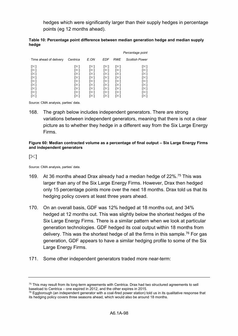
A6.1A-98

hedges which were significantly larger than their supply hedges in percentage

points (eg 12 months ahead).

Table 10: Percentage point difference between median generation hedge and median supply hedge

Percentage point

Time ahead of delivery Centrica E.ON EDF RWE Scottish Power

[] [] [] [] [] [] [] [] [] [] [] [] [] [] [] [] [] [] [] [] [] [] [] [] [] [] [] [] [] [] [] [] [] [] [] [] [] [] [] [] [] [] [] [] [] [] [] [] [] [] [] [] [] []

Source: CMA analysis, parties’ data.

168. The graph below includes independent generators. There are strong

variations between independent generators, meaning that there is not a clear

picture as to whether they hedge in a different way from the Six Large Energy

Firms.

Figure 60: Median contracted volume as a percentage of final output – Six Large Energy Firms and independent generators

[]

Source: CMA analysis, parties’ data.

169. At 36 months ahead Drax already had a median hedge of 22%.75 This was

larger than any of the Six Large Energy Firms. However, Drax then hedged

only 15 percentage points more over the next 18 months. Drax told us that its

hedging policy covers at least three years ahead.

170. On an overall basis, GDF was 12% hedged at 18 months out, and 34%

hedged at 12 months out. This was slightly below the shortest hedges of the

Six Large Energy Firms. There is a similar pattern when we look at particular

generation technologies. GDF hedged its coal output within 18 months from

delivery. This was the shortest hedge of all the firms in this sample.76 For gas

generation, GDF appears to have a similar hedging profile to some of the Six

Large Energy Firms.

171. Some other independent generators traded more near-term:

75 This may result from its long-term agreements with Centrica. Drax had two structured agreements to sell baseload to Centrica – one expired in 2012, and the other expires in 2015. 76 Eggborough (an independent generator with a coal-fired power station) told us in its qualitative response that its hedging policy covers three seasons ahead, which would also be around 18 months.

A6.1A-99

ESB’s median hedge was zero a week ahead of delivery.77

At six months ahead of delivery, Intergen’s median hedge was zero.78

We have limited data for MPF, because it bought its plants only in the last

couple of years. [].

172. As noted in the main body of this appendix, there are several reasons why

Drax and GDF may hedge differently from other independent generators.

Generation hedging – daily shape

173. We see a similar picture for the hedging of daily shape in generation as in

supply. Most of the Six Large Energy Firms seem to hedge using only

Baseload and Peak until close to delivery.79 Many firms fully shape their

positions only at the day-ahead stage, although some firms appear to do

some hedging using forward blocks.80 The graph below shows [] hedging –

the flat lines suggest it trades only (or primarily) Baseload and Peak products

until around a week before delivery.

Figure 61: Median contracted volume by settlement period – []

[]

Source: CMA analysis, party’s data.

174. Independent generators also seem to hedge primarily using Baseload and

Peak in forward markets. This is shown in the graph below for GDF. We can

also see that GDF hedged a small amount using Blocks six months ahead.

Figure 62: Median contracted volume by settlement period – []

[]

Source: CMA analysis, parties’ data.

175. Overall, generators do not seem to be hedging using fully shaped products.

Both the Six Large Energy Firms and independent generators appear to leave

their shape hedging until near to delivery.

77 ESB is currently only hedging its Corby power station. This was built in 1993 (DECC (2014) Electricity: chapter 5, Digest of United Kingdom energy statistics (DUKES), 5.10: Power stations in the United Kingdom), meaning that it probably has low efficiency. It is therefore hard to predict whether it will run. ESB may therefore have little need to trade forward the output from this plant. ESB’s data is consistent with its statement that it trades Corby’s output only up to month ahead. 78 []. 79 [] graph is different, as it includes some signs of shape. However, this seems to be the result of eight months (August 2011 to March 2012) of trading in its coal portfolio only. 80 [].

A6.1A-100

Effects of vertical integration

176. Up to this point, our analysis has looked at the generation and supply arms of

the Six Large Energy Firms separately. In this section, we consider these

parts of their businesses together. In particular, this allows us to consider the

potential effects of the natural hedge between generation and supply

activities.

177. We asked each of the Six Large Energy Firms whether their supply arm

considers their generation arm when hedging (and vice versa). Most of them

said that their different arms make these decisions independently. []. RWE

stated that ‘When the Supply Business evaluates the extent to which it is

hedged at various points ahead of delivery, no consideration is given to the

Generation Business positions.’

178. Some of the Six Large Energy Firms did identify situations where they

consider different arms together for the purposes of hedging, based on

overarching risk assessments:

(a) [];

(b) [];and

(c) E.ON said that ‘The supply business has at times considered our

generation position when considering the degree of strategic risk we face.’

179. We also have an example of wider considerations from [].

180. Taking the statements from the Six Large Energy Firms into account, we

looked at the extent to which factoring in generation activities affects the

degree to which these firms are hedged. We did this by constructing a

measure we called total hedge, which applies to the firm’s supply business.

This adds together the contracted volumes purchased by the supply business

and the firm’s uncontracted generation. The total hedge is expressed as a

percentage of the firm’s final volume supplied. This is only an indicative

metric. (See the section titled ‘the Natural Hedge’ in the main body of this

appendix.)

181. As the example chart below shows, the composition of the total hedge

changes over time. At three years out, [] total hedge is dominated by

uncontracted generation. Over time, there are more supply purchases, and

there is less uncontracted generation.

A6.1A-101

Figure 63: Total hedge by source – EDF Energy

[]

Source: CMA analysis, party’s data.

182. The chart below shows the median total hedge for the Six Large Energy

Firms. The slope is fairly flat, meaning that each firm starts off with a

significant total hedge. For example, at 24 months out, each firm has a total

hedge of at least 49%, and three firms have a total hedge of over 92%.

Figure 64: Median total hedge (uncontracted final generation plus supply contracts, as a percentage of final demand) – Six Large Energy Firms

[]

Source: CMA analysis, parties’ data.

183. Although this applies at the median, it would still be possible for there to be

periods with a low total hedge. This could occur if the output profile from a

firm’s generation deviated significantly in places from the demand profile of its

supply business. This does not appear to be the case. Even at the lower

quartile, each firm still has a significant hedge in place. With the exception of

[], each firm had a lower quartile total hedge of at least 40% at all

timescales.

184. The total hedge metric helps us to remember that the supply hedge of the Six

Large Energy Firms may look rather different if we consider the impact of

uncontracted generation. It may be harder for a non-integrated supplier to

achieve the same total hedge as a vertically integrated supplier, as this would

require larger amounts of purchases along the curve.

Gas supply hedging

185. As a comparison, we can look at the hedging of firms in the gas market. As

noted in the main section of this appendix, there are some key differences

between gas and electricity that could affect firms’ hedging in the two

products.

Volumetric gas supply hedging

The Six Large Energy Firms

186. Four of the Six Large Energy Firms had very similar hedging profiles. Each

was around 10% hedged 24 months ahead, and 40–45% hedged 12 months

ahead. This means that these firms were buying the majority of their volumes

within year.

A6.1A-102

Figure 65: Median contracted volume as a percentage of final demand – gas supply – Six Large Energy Firms

[]

Source: CMA analysis, parties’ data.

187. The exception (for whom we had data) was [], which was over [] hedged

[] months out. [] noted in its response to the supply questionnaire that its

[].

188. The Six Large Energy Firms have smaller offsetting upstream positions in gas

than in electricity, or in some cases none in gas.81 If the ‘natural hedge’ were

important for firms’ hedging decisions in electricity, then we might expect them

to react by explicitly hedging larger volumes in gas, so as to achieve the same

overall effect. This does not appear to be the case.

189. Looking at the hedged percentages, apart from [], firms generally had

larger hedges for electricity than for gas. The only exceptions were [], and

[].82 This can be seen in the chart below, where the percentage point

difference between electricity and gas is generally positive (meaning that the

median percentage hedge is larger in electricity).

Figure 66: Percentage point difference: median contracted volume as a percentage of final demand in electricity, minus median contracted volume as a percentage of final demand in gas – Six Large Energy Firms

[]

Source: CMA analysis, parties’ data.

Independent suppliers

190. The graph below adds the hedging profiles for independent suppliers. It

appears that independent suppliers had somewhat shorter gas hedging

profiles than the Six Large Energy Firms.

Figure 67: Median contracted volume as a percentage of final demand – gas supply – Six Large Energy Firms and independent suppliers

[]

Source: CMA analysis, parties’ data.

191. Neither [] nor [] seemed to hedge a significant amount 24 months out

relative to their actual supply.83 In contrast, the Six Large Energy Firms all

carried out some hedging at this stage. The percentage hedged by [] was

81 See Section 4: Nature of competition in wholesale energy markets. 82 However, making direct comparisons between the hedged percentages for gas and electricity is somewhat complicated because electricity has daily shape, while gas does not. 83 [].

A6.1A-103

similar to or larger than those from the Six Large Energy Firms by the year-

ahead stage, and the percentage hedged by [] was similar to those from

the Six Large Energy Firms by six months ahead. From the data available,

[] also seemed to have a similar or larger hedge than the Six Large Energy

Firms from 12 months out. We do not have trading data for []. However,

from other information submitted, we understand that it carries out the

majority of its hedging within a year from delivery.84

192. If liquidity were the key constraint preventing independent suppliers from

trading forward in electricity, then we might expect to see independent

suppliers trading further ahead in gas. However, there is a mixed picture on

this. [] gas hedges were all larger than the equivalent electricity hedges.

[] gas hedges were larger 18 months out [] and 12 months [].

However, none of [] gas hedges was larger than its electricity equivalents.

As with Figure 66, a bar above the axis indicates that the median percentage

hedge is larger in electricity than gas.

Figure 68: Percentage point difference: median contracted volume as a percentage of final demand in electricity, minus median contracted volume as a percentage of final demand in gas – independent suppliers

[]

Source: CMA analysis, parties’ data.

Gas supply hedging – annual shape

193. We also looked at how firms manage their annual shape in gas. We might

expect this to be more significant in gas than electricity, given that season

variation in gas demand is substantially greater than in electricity.

194. As in electricity, Centrica, [] and [] appear to be leaving their monthly

shaping until closer to delivery. As the graph below shows, [] supply hedge

started to mirror its monthly shape only between six months and one month

before delivery. This would be consistent with [] hedging using mainly

products longer than a month (ie Quarters and Seasons) before that point.

Figure 69: Median daily contracted volume by month in summer – [] gas supply

[]

Source: CMA analysis, party’s data.

195. As with electricity, E.ON’s graph had monthly shape from an early stage.

E.ON is able to buy Monthly gas products from its trading business up to six

84 Based on charts submitted as part of its response to our electricity questionnaire.

A6.1A-104

seasons ahead. In the case of gas, [] also had a contracted monthly shape

which followed the pattern of demand [].85

Figure 70: Median daily contracted volume by month in summer – [] gas supply

[]

Source: CMA analysis, party’s data.

196. All three of the independent suppliers for which we have data ([]) also had

profiles that exhibit some monthly shape. []. These positions may result

from independent suppliers being able to trade a more granular product range

through their intermediaries.

Figure 71: Median daily contracted volume by month in summer – [] gas supply

[]

Source: CMA analysis, party’s data.

Trading in support of hedging

197. In this section we bring together information on trading and hedging to assess

whether the external trading carried out by the Six Large Energy Firms is

sufficient to construct their hedged positions. If this trading is sufficient, then it

suggests that independent firms should be able to replicate these hedges in

the market. If the Six Large Energy Firms’ external trading is not sufficient,

then this might indicate that internal trading plays an important role. This

would be an option unavailable to independent firms (without either vertically

integrating or entering into a long-term contract with a generator willing to

trade shape well in advance of delivery).

Comparing hedging and trading – volumetric hedging

198. While our hedging and trading data cover similar timeframes, they are not

immediately comparable. For example, our trading data includes all trades,

whereas the hedging data looks only at snapshot days. We therefore

converted the hedging data into an annual hedge volume requirement. This

involves transforming the median hedged volume per settlement period into

an annual purchase requirement.86

199. We then compared this against (for supply) the annual average volume

bought and (for generation) the annual average volume sold, based on the

85 [] had [] long-term contracts active throughout the period. Of these, []. The remaining [] contracts have []. However, while [] has some [], we do not know whether it has used these contracts to achieve monthly shape. 86 Multiplying by 17,520 (number of half-hour settlement periods per year).

A6.1A-105

trading data we collected. The graph below presents the volumes bought and

sold on a cumulative basis. This is for comparability with the hedge profiles,

which build up over time.

200. This analysis is necessarily approximate, with several caveats:

(a) The hedge volume requirement will be a slight overestimate. This is

because the hedging data covered only Tuesdays, and weekends have

lower demand.87

(b) The hedged volume is based on the time until a particular delivery date,

whereas the traded volume is categorised by the time until a product

starts delivering. As the categorisation is stricter for traded volume, this

will also tend to make the hedge volume requirement harder to meet.

(c) For the supply comparison, the traded volume is based on purchases. In

reality the supply arm will sell as well as buying, but we cannot identify

which trades were carried out for supply purposes. (Similarly, the

generation arm will sometimes buy as well as selling.)

201. The question we ask is whether the traded volume meets (or exceeds) the

hedge volume requirement. If not, then (subject to the caveats above) this

would suggest that some of the hedge is being achieved through internal

transfers. The caveats are largely conservative (ie they make the hedge

volume requirement harder to meet).

202. We are able to complete this analysis for five of the Six Large Energy Firms.88

For each company, we look at generation and supply separately, so we have

ten graphs in total. We discuss the results in more detail below, but we

summarise the results here:

(a) Two graphs ([]) show traded volume exceeding the hedge volume

requirement in every timeframe.

(b) Three graphs ([]) show traded volume exceeding the hedge volume

requirement in all but one or two timeframes. In the cases where the

traded volume is lower, this is only by small amounts (under 2TWh).

(c) Three graphs ([]) have four instances where the traded volume is less

than the hedge volume requirement. However, the differences are not

particularly large.

87 This may not be significant if most trading along the curve is Baseload. 88 We cannot look at SSE in this way, because it was unable to complete our hedging templates.

A6.1A-106

(d) Two graphs ([]) show the traded volume exceeding the hedge volume

requirement only from month ahead. The traded volume can also be

significantly lower than the hedge volume requirement (by up to 18TWh).

203. In general, this suggests that trading activity is sufficient to deliver parties’

hedged positions, and even where it does not cover the complete hedged

volume, there is substantial trading activity at each point in time where the

firm takes a hedged position.

204. []. This suggests that [] trading is generally consistent with its hedging.

Figure 72: Comparing cumulative volume bought and volume required to achieve hedge – [] supply

[]

Source: CMA analysis, party’s data.

205. [].

Figure 73: Comparing cumulative volume sold and volume required to achieve hedge – [] generation

[]

Source: CMA analysis, party’s data.

206. E.ON’s supply hedge volume requirement []. The largest difference is at

[] out in volume terms (nearly [] of the hedge volume requirement).

Figure 74: Comparing cumulative volume bought and volume required to achieve hedge – [] supply

[]

Source: CMA analysis, party’s data.

207. For E.ON’s generation business, the volume it sold was also []. However,

the differences were fairly small (up to [] difference).89

Figure 75: Comparing cumulative volume sold and volume required to achieve hedge – [] generation

[]

Source: CMA analysis, party’s data.

208. [].

89 As with E.ON’s supply business, the largest difference in percentage terms was 36 months out (91%). However, this was also based on very small volumes.

A6.1A-107

Figure 76: Comparing cumulative volume bought and volume required to achieve hedge – [] supply

[]

Source: CMA analysis, party’s data.

Figure 77: Comparing cumulative volume sold and volume required to achieve hedge – [] generation

[]

Source: CMA analysis, party’s data.

209. The graph below shows that RWE [].

Figure 78: Comparing cumulative volume bought and volume required to achieve hedge – [] supply

[]

Source: CMA analysis, party’s data.

Figure 79: Comparing cumulative volume sold and volume required to achieve hedge – [] generation

[]

Source: CMA analysis, party’s data.

210. [] almost entirely met the hedge volume requirement for its supply business.

[]. The difference was [], and arose because it had a [].

Figure 80: Comparing cumulative volume bought and volume required to achieve hedge – [] supply

[]

Source: CMA analysis, party’s data.

211. [].

Figure 81: Comparing cumulative volume sold and volume required to achieve hedge – [] generation

[]

Source: CMA analysis, party’s data.

Comparing hedging and trading – annual shape

212. Independent suppliers have suggested that there is limited liquidity in Monthly

products further along the curve.90 The Six Large Energy Firms do not appear

90 For example, see paragraph 13.

A6.1A-108

to do much trading of Monthly products along the curve (as there is little

volume traded beyond three months out).91

213. However, the Six Large Energy Firms also do not seem to be hedging using

Monthly products along the curve. We have already looked at [] supply

hedging of annual shape.92 The charts below add to this by showing hedging

by the supply businesses of [] and [] on a monthly basis during the

summer.93 In each case, the contracted volume in September is higher than

the contracted volume in April in timescales up to six months ahead. This is in

contrast to the profile of demand, which is higher in April.94 This suggests that

these parties are not hedging using monthly products until within six months

from delivery, which is in line with their trading data. The picture for [] is

generally similar (eg at 12 months ahead of delivery).

Figure 82: Median contracted volume per settlement period by month in summer – [] supply

[]

Source: CMA analysis, party’s data.

Figure 83: Median contracted volume per settlement period by month in summer – [] supply

[]

Source: CMA analysis, party’s data.

Figure 84: Median contracted volume per settlement period by month in summer – [] supply

[]

Source: CMA analysis, party’s data. Note: [].

214. []. This allows it to obtain []. For example, its contracted monthly profile at

[] before delivery is broadly similar to the shape of monthly demand.

Figure 85: Median contracted volume per settlement period by month in summer – [] supply

[]

Source: CMA analysis, party’s data.

Comparing hedging and trading – daily shape

215. Our trading data showed that most Peak is traded within a year from delivery

by the Six Large Energy Firms (although all of them trade small volumes

further down the curve).

91 See Figure 6 (Monthly Baseload) and Figure 9 (Monthly Peak). 92 See Figure 49. 93 As we do not have the full data for summer 2014, we exclude it from this analysis. 94 Approximated on the graph by the contracted volume at delivery.

A6.1A-109

Figure 86: Volume of trading by time ahead of delivery by the Six Large Energy Firms – Peak

[]

Source: CMA analysis, parties’ data.

216. This is aligned with the charts below, which show the median contracted

volume by settlement period at each stage ahead of delivery. From these, we

can see when five95 of the Six Large Energy Firms start to hedge their supply

businesses’ daily shape.

217. [] and [] both start to have evidence of Peak hedging only at 12 months

ahead of delivery. This corresponds to their trading above – both companies

traded some Peak between 12 and 18 months from delivery. Both firms also

have Peak hedges that increase closer to delivery. This matches the build-up

of traded volume over time.

Figure 87: Median contracted volume by settlement period – [] supply

[]

Source: CMA analysis, party’s data.

Figure 88: Median contracted volume by settlement period – [] supply

[]

Source: CMA analysis, party’s data.

218. Similarly, the chart below shows [] supply hedging. [] pro file includes

some []. Figure 20 showed that [] traded some volume in ‘other standard

products’ (a category including Extended peak and Overnights) between 18

and 24 months ahead, making it possible that [] achieved this shape in the

market.

Figure 89: Median contracted volume by settlement period – [] supply

[]

Source: CMA analysis, party’s data.

219. [] appears to add daily shape at a later stage []. Its graph indicates that it

is hedging shape only at []. This is consistent with the trading graph, which

suggests [] is trading only small volumes of Peak along the curve.

Figure 90: Median contracted volume by settlement period – [] supply

[]

95 As previously, we do not have this data for SSE.

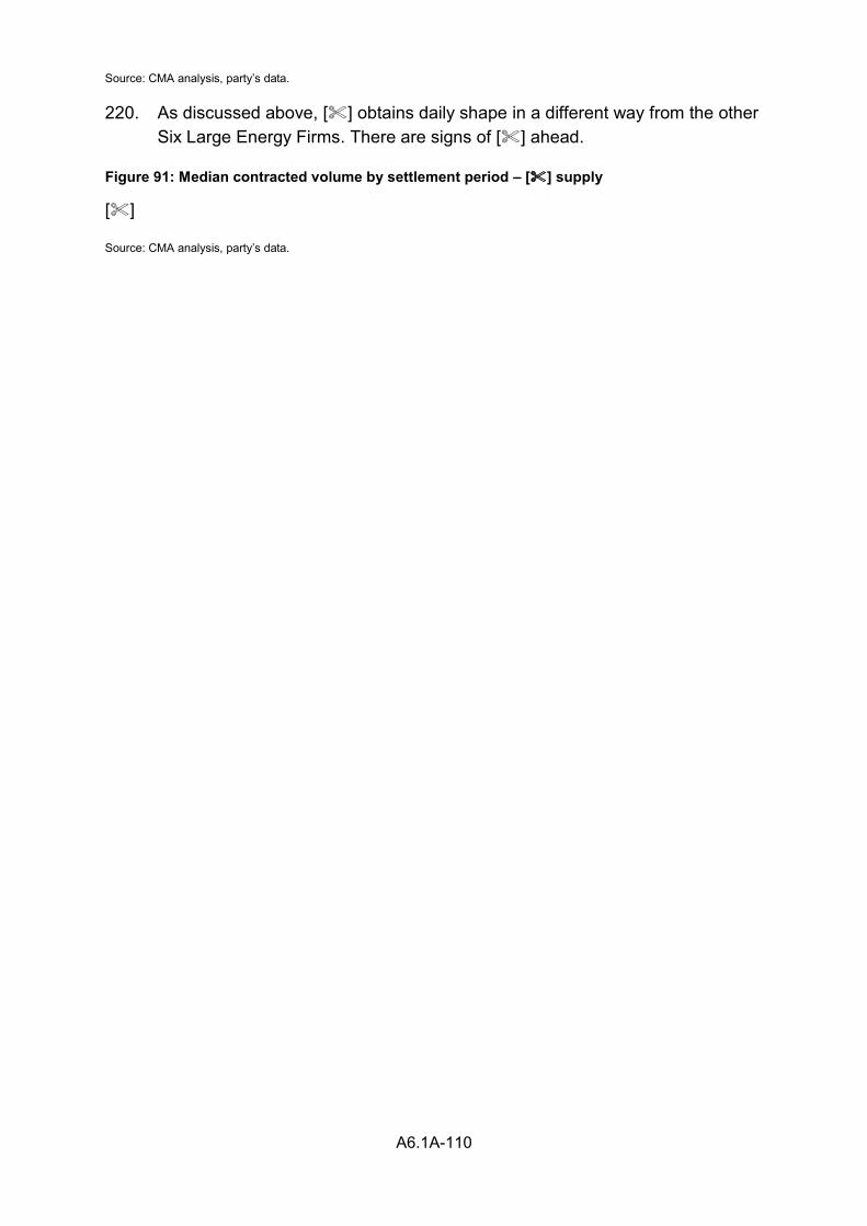
A6.1A-110

Source: CMA analysis, party’s data.

220. As discussed above, [] obtains daily shape in a different way from the other

Six Large Energy Firms. There are signs of [] ahead.

Figure 91: Median contracted volume by settlement period – [] supply

[]

Source: CMA analysis, party’s data.