annual report (year two) on the habitat evolution mapping project for … · 2011-07-15 · annual...

Annual Report (Year Two) on theHabitat Evolution Mapping Project

for theSouth Bay Salt Pond Restoration Project

Submitted by:

Brian FulfrostProject Manager

Habitat Evolution Mapping ProjectBrian Fulfrost and Associates

July 6th, 2011

July 6th, 2011

Annual Report (Year Two) on theHabitat Evolution Mapping Project

for theSouth Bay Salt Pond Restoration Project

Submitted by

Brian Fulfrost, Project Manager

South Bay Salt Pond Restoration – Habitat Evolution Mapping Project

Brian Fulfrost and Associates

56 Rio Vista Ave

Oakland, CA 94611

831-566-7686

Summary of Work Completed

This report outlines the work conducted during Year Two (April 2010 – April 2011) of the Habitat

Evolution Mapping Project (HEMP). In Year Two (2010) the HEMP team successfully utilized an

improved version of the habitat model to map over 15,000 acres of marsh habitats and mudflats in the

south bay of San Francisco. We spent considerable amount of time improving the habitat model's

overall accuracy (already at 80% attribute accuracy) from Year One and providing the necessary data

for tracking changes to habitats within the study area, including ponds already breached for restoration

(see Figures 1,2 and 3). Improvements in Year Two focused on increased efficiency in ground truthing,

changes to the mix of habitats being mapped, and tweaks to image classification methods. Although

there was some delays in receiving the Ikonos imagery within specification, there were no significant

delays from reporting, permitting or equipment that were previously encountered during Year One. As

a result, there were additional improvements in overall project efficiency, Ikonos imagery acquisition

timing, the effectiveness of our ground truthing, as well as in our final Year Two model results.

Status of Mapping Products

Habitat Classes

The list of habitats being classified in the model was further refined in Year Two, based on a number of

factors. These include the effectiveness of a given habitat class during a model run, the spectral

similarity (or difference) between a given habitat and another, the image characteristics of certain

vegetation associations or habitats, , and ultimately the importance to overall project goals. Changes to

the list of habitats being mapped were vetted in consultation the South Bay Salt Pond Restoration

(SBSP) Project Management Team (PMT) and US Fish and Wildlife Service (USFWS) biologists at

Don Edwards National Wildlife Refuge.

Biofilm

After reviewing the results of our initial habitat classifications during Year Two, it became clear that

there were “out of place” biotic signatures appearing on mudflats in both the 2010 and 2009 imagery

(Type I errors of other habitats not found on mudflats, notably Gumplant). These areas either did not

normally contain macrophytic plant species (on the mudflats themselves) or plant species of this type

(high marsh plants vs. low marsh plants). Dr. John Takekawa (USGS) and other researchers identified

that the likely source of these signatures was “biofilm” occurring on the surface of tidal mudflats. This

1 Year Two Annual Report

biofilm might potentially serves as an important source of food for bird populations important to the

restoration effort. As a result, the HEMP team and the SBSP PMT decided to add biofilm to the list of

priority habitats to be mapped.

We obtained ground truthed locations of biofilm in order to generate training sites to map the extent

and distribution of these types of mudflats throughout the study area. The result of adding biofilm to

our list of habitats classes, include:

• a validated map of biofilm distribution on mudflats throughout the study area (within breached

ponds, along sloughs and even within marshes); and

• a significant improvement in overall model accuracy especially within breached ponds.

After subsequent conversations with the USGS team studying biofilm at Dumbarton shoals, it was clear

that (a) the lack of water on top of and exposure of mudflats to the sun resulted in potentially higher

probability of biofilm; and (b) there were a range of type of biofilms which could be descriptively

characterized by density. We are not confident that our ground truthing locations adequately represent

this variability and therefore we can not be certain if the model is mapping the complete distribution of

biofilm.

By the end of Year Two, the model contain a total of 25 unique “habitats” (see Table 1 and Table 2).

These are the various biotic (e.g.“Pickleweed”) and abiotic (e.g. “mud”) land cover classes that are

mapped as part of the project. The biotic habitat classes include: 10 salt marsh, 4 brackish, and 3

freshwater vegetation associations. Although the focus of the project is on vegetation, and vegetation

associations (e.g. Pickleweed /- Cordgrass), the term “habitat” is being used here to refer to both biotic

and/or abiotic land cover classifications.


Table 1: Marsh Habitat Classifications

Salt Marsh

Community

Salt Marsh

Vegetation

Brackish Marsh

Vegetation

Freshwater Marsh

Vegetation

low

Pickleweed (annual) Alkali Bulrush BulrushCordgrass Alkali Bulrush /-

Pickleweed

Cattail

low - mid Pickleweed /- Cordgrass Alkali Bulrush /-

Pepperweed

Bulrush /- Cattail

mid

Pickleweed /- Saltgrass Alkali Bulrush /-

SpearscalePepperweedPickleweed /- Pepperweed

Pickleweed /- Jaumea

mid - high

Pickleweed (perennial)

Pepperweed

high Alkali HeathGumplant /- Pickleweed

Table 2: Non-Vegetated and Upland Habitat Classifications

Non-Vegetated Upland (and ecotone)

Mudflat Alkali GrassesMudflat with Biofilm MustardAlgae SaltgrassWrack Alkali HeathBare Earth PepperweedWater


Ground Truthing

In Year Two, we surveyed 172 locations using one of our standardized ground truthing protocols and

noted the vegetation and other land cover characteristics at an additional 331 locations (see Map 1).

David Thomson, the lead biologist on the HEMP tam, conducted the majority of our ground truthing

surveys. These ground truthing datasets served a number of functions:

• evaluating the number and type of habitats being mapped,

• assisting with the qualitative review of model results,

• identifying new or modified training sites for various versions of the model, and

• final model validation.

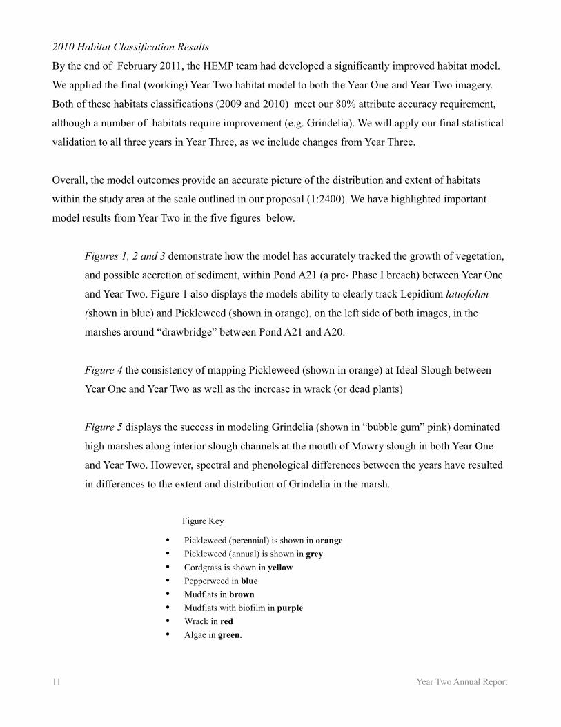
As in the previous year, we continued to utilize the Trimble Yuma (with Trimble Terrasync for data

collection) with a Trimble ProXT external antenna for obtaining sub-meter GPS locations of our

ground truthing sites. During Year Two, modifications were made to the Terrasync “data dictionaries”

(i.e. our digital field survey forms) as necessary and as suggested by our lead biologist, David

Thomson. Significant time was also spent in cleaning and combining our ground truthing datasets so

they could be used more efficiently. We used ground truthing surveys to assist with developing new or

modified trainings sites for the habitat model as well as for model validation.

Rapid Assessments

Between June and August, we conducted 69 additional rapid assessments to assist with supplementing

our knowledge of vegetation associations and phenological variability throughout the study area.

Model Calibration

Between June and September, we also conducted 30 ground truthing surveys (a simplified form of

Rapid Assessments) to assist with calibrating the model results.

Validation

Unlike Year One, we were successful in obtaining a stratified random sample of 73 habitats on the

ground for statistical validation of the model. In order to identify the locations for our validation

surveys, we generated a random sample of 200 points stratified (by area) into the following categories:

salt marsh, brackish marsh, fresh marsh, and managed marsh. Our validation focused ground truthing


occurred between October 2010 and November 2010. Unfortunately, due to time and weather changes,

we were only able to survey a little more one-third of these 200 locations. As a result, we supplemented

our validation sample with ground truthing surveys obtained from our rapid assessments and model

calibration during Year Two.

The table and chart below, which do not include supplementary data and exclude data collected on

levee tops, help to characterize the type and variability of dominant vegetation associations among salt,

brackish and fresh marshes within the study area. Table 3 below lists the number of occurrence and

type of dominant vegetation associations obtained from our ground truthing (excluding our

supplementary ground truthing dataset) . Chart 1 proportionally divides the various types of vegetation

associated with Pickleweed (perennial) obtained from our ground truthing in Year One and Year Two.


Table 3: Number of Occurrences of Dominant Vegetation Associations (Year One and Year Two)

Chart 1: Pickleweed Associations (Year One and Year Two)

We achieved approximately 80% attribute accuracy using a total of 172 points for our preliminary

validation drawn from these three ground truthing surveys. Once we have filtered and cleaned our

supplementary ground truthing surveys, we will use these additional locations to expand our final

validation sample size for Year Two (and for Year One).


Map 1: Year Two Ground Truthing Locations

Ikonos Imagery Acquisition and Processing

The 1 meter Ikonos imagery was acquired on July 4th, 2010 (Year One date was June 23rd, 2009) at 2.3

feet above MLLW, allowing for maximum exposure of vegetation and mudflats as well as reduced

moisture content in the vegetation. The image was acquired on the second attempt (out of a possible 3)

since the first image capture contained too much cloud cover and was out of specification.

The HEMP team selects 3 days in June or July, when tidal marsh vegetation is near peak growth. (In

order to select specific days the project pays a “tasking fee” to secure the satellite on days the company

say its available.) The IKONOS satellite passes over the study area around noon to minimize shadows

and glint from the sun. Our optimal acquisition days are when the lower-low tide occurs 1-hour before

noon and the predicted tidal depth is less than 1 foot above ( or below) the station’s MLLW datum. We

optimally want one hour after lower-low tide because there is a delay in the tidal cycle from North to

South “up-estuary”, which is roughly ½-hour between the San Mateo Bridge and Alviso. As a result,

during the hour following an ebb tide the tidal depths across the study area will be more equivalent

because northern areas will be in slack tide (i.e. not changing) for at least an hour while the southern

portion reaches low slack tide. However, since days at which the Ikonos satellite will overpass do not

always match with these optimal dates, we had to loosen our criteria to 1 hour before or after lower-low

tide and a predicted tidal depth of less then 1 meter.

The HEMP team, in consultation with the SBSP PMT, also considered switching to the higher

resolution GeoEye1 satellite for Year Two but stayed with Ikonos to ensure consistency for the time

period of the study. The GeoEye1 also lacks operational bi-directionality and therefore it is more

difficult to capture the study area in a single pass.

The Ikonos imagery was obtained in 3 “snapshots” from a a single pass over the study area. In Year

Two, the Ikonos imagery was delivered in two orthorectified image formats: (1) as a single 1 meter

pan-sharpened image mosaic (of the 3 “snapshots”) that have been radiometrically processed for image

clarity; and (2) as 3 individual “strips” containing the “raw” Digital Numbers (DN) for both the 4 meter

multispectral and 1 meter panchromatic bands. The pan-sharpened image mosaic is used for all general

mapping needs as well as our crucial qualitative model review. The “raw” data, contains unmodified

values which have not been radiometrically corrected (e.g. DRA), pan-sharpened, or mosaiced. As a

result these image strips contain non altered (or “raw”) image values (also called “digital numbers” or

DN) and are consequently used for image normalization, habitat classification and change analyses.


Unfortunately, the imagery was delivered out of specification with regards to positional accuracy and

as a result we didn't receive the final satellite imagery (within 2 - 4 meters) until late August 2010.

Image processing in Year Two focused on (1) developing standardized methods for normalizing and

correcting the Ikonos imagery for applying the model to allow for consistency of mapping over time as

well as for performing change analyses; and (2) improvements to the accuracy of spectral habitat

model developed in Year One. Erdas Imagine 9.3 continued to be used for all image processing, habitat

model refinements, and image classification.

Image Masking

Once we received the final Ikonos imagery for Year Two, we utilized the inclusion/exclusion mask to

generate imagery that include only the area within the project boundary actually being mapped. This

assist in both qualitative model interpretation by reduction the area b being classified as well as

qualitative image classification by only including the elements of the baylands that the spectral model

is classifying.

The HEMP team spent some time editing the boundaries of our image “mask” to better comply with a

actual marsh and pond boundaries. This mask has 3 versions, all of which cover the exact same area:

(1) an inclusion/exclusion mask for areas within the image that are being mapped as part of the project;

(2) the inclusion/exclusion mask divide into the following categories: salt marsh, brackish marsh, fresh

marsh, and managed marsh; and (3) the inclusion mask divided up into a number of habitat types from

the original sources of the mask (Habitat Goals, 1998; Existing Conditions – 2004; HT Harvey

Vegetation Mapping of Guadalupe Slough – 2008). Once the Bay Area Aquatic Resource Inventory

(BAARI) being developed by SFEI is released, we will utilize it to further refine this mask as needed

for Year Three.

Image Normalization

Year Two introduced additional processing requirements required for radiometric normalization of the

images in both (and subsequent) years.

The HEMP team spent a considerable amount of time in the Fall 2010 attempting to normalize the

Ikonos imagery from both Year One and Year Two. The preferred method would be to utilize an

absolute image-based atmospheric correction method such as Cosine of Sun Zenith Angle (COST) or

Dark Object Subtraction (DOS) so as to convert the at senor radiance to actual ground reflectance. An


alternative and acceptable image based atmospheric correction method would be to utilize the

standardized exoatmospheric correction (in essence “planetary reflectance” vs. ground reflectance)

developed for Landsat imagery and commonly applied to Ikonos imagery. Unfortunately, although

significant project time was spent on applying various image based atmospheric correction methods to

the Ikonos imagery, we were unsuccessful at achieving acceptable results using any of these methods.

In a effort to continue to make progress towards our goals, we utilized an alternative relative

normalization method (as opposed to absolutely correcting for atmospheric disturbance) known as

histogram matching. This is an image based correction method in which we use a “base year”, in this

case our 2009 image, and match the histograms of subsequent years to the base year in an effort to

normalize the spectral variability of images over time. The advantage of this method is it is easy to

implement. The disadvantage is this method does not account for atmospheric effects. In the end, we

matched the histograms of each 2010 Ikonos strip to the corresponding strip from 2009 resulting in

accurate model results for each year. Although our image normalization was successful, it was not

perfect. As a result, there continue to be radiometric differences between the image years that introduce

some error into the application of the model.

Supervised Classification Review and Habitat Model Refinements

Once the images were normalized, we ran the most current version of the habitat model on both the

2009 and normalized 2010 (raw) image strips (3 total for each year). As in Year One, we utilized a

“maximum likelihood” supervised classification. In the final working version of the Year Two model

we also added probabilities (in the form of statistical weights) to specific habitat training sites (e.g.

Gumplant) based on the type of error (I or II) and/or level of accuracy of a given habitat. This greatly

improved the overall accuracy of the mapping results for “difficult” habitats such as Gumplant.

ArcGIS continued to be used for our qualitative model review, digitizing training sites, as well as for

statistical validation.

Improvements to the habitat model were made iteratively, as we performed our qualitative review of

the results of a given model results and as we ground truthed additional areas and habitats. Changes to

the model resulted in the increased accuracy of individual habitats and improvements to the “mix” of

various vegetation associations being mapped. These improvements resulted from introducing training

sites that captured the adequately habitat and phenological variability in the study area and were

spectrally 'distinct' enough to be mapped as distinct habitats.


Since the habitat model consists of a series of training site(s) for each habitat class (that are used to

represent the “spectral signature” for each habitat being mapped), the primary mechanism for

implementing these changes was either to alter existing training sites or to intrude new and/or multiple

training sites for each habitat. A significant amount of project time was spent in the process of model

review and model refinement. In the end, dozens of models were developed with various numbers of

and types of habitats.

Necessary improvements to the model were identified as we obtained more data (primarily from

ground truthing) regarding the spatial, vegetative, and phenological variability of habitats. As a result

we better understood the spectral differences (or similarity) of a particular habitat. As the list of habitats

being mapped changed we discussed these changes with appropriate USFW&S staff to ensure that the

mapped habitats would still ultimately meet project goals. For example, although mapping the extent

and distribution of Iceplant (both Carpobrotus sp. and Mesembryanthemum nodiflorum ) would be

useful to the restoration effort (in in effort to understand its impact on marsh vegetation dynamics), it's

spectral similarity to Pickleweed resulted in significant Type I errors (false positive) where Iceplant

was erroneously displacing large amounts of Pickleweed . As a result, we excluded this species from

our model during Year Two, resulting in increased accuracy of other priority habitats (notably

Pickleweed).

As in previous years, the HEMP team qualitatively assessed the accuracy of a given model's results,

utilizing the following resources:

• existing ground truthing datasets (from HEMP, ISP, HT Harvey),

• Bing Maps (oblique view),

• our habitat interpretation guide,

• and expert knowledge of the study area.

Additional ground truthing surveys were obtained to calibrate the model during their qualitative

review as the image interpreter identified problematic or questionable habitat assignments. Details

about the protocols and procedures used for our qualitative review have been explained elsewhere (see

HEMP Year One Annual Report) and will be documented in our final report.


2010 Habitat Classification Results

By the end of February 2011, the HEMP team had developed a significantly improved habitat model.

We applied the final (working) Year Two habitat model to both the Year One and Year Two imagery.

Both of these habitats classifications (2009 and 2010) meet our 80% attribute accuracy requirement,

although a number of habitats require improvement (e.g. Grindelia). We will apply our final statistical

validation to all three years in Year Three, as we include changes from Year Three.

Overall, the model outcomes provide an accurate picture of the distribution and extent of habitats

within the study area at the scale outlined in our proposal (1:2400). We have highlighted important

model results from Year Two in the five figures below.

Figures 1, 2 and 3 demonstrate how the model has accurately tracked the growth of vegetation,

and possible accretion of sediment, within Pond A21 (a pre- Phase I breach) between Year One

and Year Two. Figure 1 also displays the models ability to clearly track Lepidium latiofolim

(shown in blue) and Pickleweed (shown in orange), on the left side of both images, in the

marshes around “drawbridge” between Pond A21 and A20.

Figure 4 the consistency of mapping Pickleweed (shown in orange) at Ideal Slough between

Year One and Year Two as well as the increase in wrack (or dead plants)

Figure 5 displays the success in modeling Grindelia (shown in “bubble gum” pink) dominated

high marshes along interior slough channels at the mouth of Mowry slough in both Year One

and Year Two. However, spectral and phenological differences between the years have resulted

in differences to the extent and distribution of Grindelia in the marsh.

Figure Key

• Pickleweed (perennial) is shown in orange• Pickleweed (annual) is shown in grey• Cordgrass is shown in yellow• Pepperweed in blue• Mudflats in brown• Mudflats with biofilm in purple• Wrack in red• Algae in green.


2009 2009 model 2010 2010 model

12 Year Two Annual ReportFigure 2: Growth in Pickleweed in Pond A21 (2009-2010)

2009

2010

Figure 1: Growth in Pickleweed in Pond A21 (2009-2010)

April 2009 Sept 2009 May 2010 October 2010


July 2010

Figure 3: Growth in Pickleweed in Pond A21. The 4 photos appearing on top are courtesy of Cris Benton and demonstrate additional evidence for the growth of Pickelweed (both annual and perennial). The area taken in these photos is highlighted on the Ikonos imagery and model results by a yellow box.

June 2009


2010

2009

2010

2009

Figure 5: Consistency of Habitat Mapping (pickleweed, cordgrass, pickleweed/cordgrass shown in tan, and pickleweed/jaumea shown in dark purple) in Tidal Marsh outside Pond A6

Figure 4: Gumplant (high salt marsh) mapped in both 2009 and 2010 at mouth of Mowry Slough. Spectral and phenological differences between years result in variability in results.

Spectral and Phenological Variability

Differences in the spectral values for a given habitat from year to year are a result of a number of

factors, including: image details (e.g. elevation angle), radiometric normalization, and phenological

differences (spatially and temporally). As a result, there will be slight differences in the mapping of a

given habitat in certain locations (local spatial variability) from year to year. Some of this variability

represents true phenological differences (dead vegetation one year vs. alive second year) in vegetation

and therefore cannot be accounted for through automated methods alone. In Figure 6, during 2009 the

Pepperweed (in blue) was dead and therefore is being mapped as Wrack (in red) while in 2010 it was

alive and therefore is being mapped as Pepperweed. In these cases, the model is actually performing to

specification since it is accurately mapping the land cover .

We have minimized the effect of this local spatial variability by trying to optimize acquisition details

(elevation angle closer to nadir), applying an effective radiometric normalization technique, and

including training sites that account for phenological differences in vegetation. However, we will

continue to attempt to account for this variability in Year Three by optimizing one or more of these

three techniques. In addition, we will explore additional methods to account for the variability (or

similarity) of certain habitats. These methods include mapping certain species which are spectrally

similar(e.g. Alkali Heath and Spearscale) as one habitat as well as identifying clear “thresholds of


2009

2010

Figure 6: Differences in phenology of Pepperweed in 2009 and 2010 (east of Pond A18)

change” (by area) for each habitat that account for this variability.

Limitations

• Mudflat Extent

The Ikonos image in Year Two was acquired at a time very close to Mean Lower Lower Water

(MLLW) and significantly improved upon the exposure and subsequent mapping of mudflats

(see below). However, the HEMP team met with key members of the PMT during Year Two at

which time it was decided that the issues involved with matching dates to which the Ikonos

satellite will pass over the study area during (or close to) MLLW limited the efficacy of using

the Ikonos imagery for mapping changes to mudflat extent..

• Levee Tops

In consultation with the SBSP PMT, the HEMP team will map “levee tops” using only two

land cover classes: (1) vegetated; or (2) non-vegetated. The mix of often weedy peripheral

halophytic vegetation that characterize levee tops have made it very difficult to accurately

distinguish between specific habitat types with any great deal of accuracy. Levee tops are

“linear” habitats that have a narrow width and often contain a complex mix of weedy

halophytic vegetation. In these cases, the imagery from the Ikonos was not capable of

accurately distinguishing individual habitats.


Year One Ikonos Year Two Ikonos

Remaining Improvements

• High Salt Marsh Habitats

The habitat model has successfully been able to delineate high marsh habitat. However, we have

been less able to accurately distinguish between certain habitats within these high salt marshes.

We have had success in distinguishing certain species, such as Alkali Heath, Jaumea, and to a

lesser degree Saltgrass.

On the other hand, we have had little success mapping Spearscale as a unique habitat often

because of its spectral similarity to other species like Alkali Heath, and the lack of good training

sites. Although certain locations of Alkali Heath might actually be Spearscale in some cases, in

either case, they are being accurately mapped as existing high salt marsh, and therefore can be

considered to be meeting project goals. On the other hand, one important species we continue to

try to accurately distinguish is Gumplant, a critical high marsh indicator species. Because of its

morphology, growth pattern (bushy along interior marsh slough channels), and association with

Pickleweed it has been often difficult to map Gumplant consistently throughout the study area

(there are a range of both Type I and Type II errors). The introduction of new or modified

training sites that represent this variability has often resulted in significant over mapping of

Gumplant. By the end of Year Two, Gumplant continues to be an area of focus for Habitat

refinement, although we are confident that our final results will be within specification.

Throughout the study area , high salt marshes are found in a number of locations within salt

marshes: 1) higher areas adjacent to sloughs often within the mid marsh; 2) higher 'mounded

areas' within the mid marsh (e.g. from natural sediment accretion or from man made features

such as historic levees), or 3) along levee flanks.


Presentations and Outreach

During Year Two, the HEMP team presented the ongoing results of the mapping project at a number of

conferences and to a number of affiliated organizations (SFEI and HT Harvey). Brian Fulfrost

presented the results of the mapping project at both the Bay Delta Conference held in Sacramento in

September 2010 and to the South Bay Salt Pond Restoration Science Symposium in February 2011. In

addition, the HEMP team continued ongoing discussions with project partners and other key

stakeholders on the project. Brian Fulfrost also provided guidance and oversight to the interns at the

NASA Develop program where students worked on a number of remote sensing projects related to the

restoration.

Year Three and Next Steps

In Year Three, we will finalize our habitat model using all 3 years worth of imagery, perform our final

statistical validation by focusing our ground truthing on validation, run change analyses on the final

model results, and document our work in our final report. We will also distinguish channels (with and

without water) and pannes as generated from the image analysis and perform manual edits to the

model results in problematic areas (or habitats).

Additional focus areas for improvement, include:

• atmospheric correction of imagery ( to potentially improve radiometric normalization),

• improvements to the final model results using two types of raster analyses:

(1) the integration of the tide/elevation raster developed by Gavin Archbald,

which will help remove blatant habitat mis-assignments according to the likelihood of

vegetation existing with a tidal/elevation range corresponding to a particular marsh

community (e.g. Gumplant in high salt marsh), and

(2) a raster based neighborhood analysis to reduce unnecessary habitat complexity.


annual report (year two) on the habitat evolution mapping project for … · 2011-07-15 · annual...

Documents