annealing techniques applied to reservoir modeling and the
TRANSCRIPT

ANNEALING TECHNIQUES APPLIED TO RESERVOIR
MODELING AND THE INTEGRATION OF
GEOLOGICAL AND ENGINEERING (WELL TEST) DATA
a dissertation
submitted to the department of applied earth sciences
and the committee on graduate studies
of stanford university
in partial fulfillment of the requirements
for the degree of
doctor of philosophy
By
Clayton Vernon Deutsch
May 1992

c© Copyright 1992 by Clayton Vernon Deutsch
All Rights Reserved
ii

I certify that I have read this thesis and that in my opin-
ion it is fully adequate, in scope and in quality, as a
dissertation for the degree of Doctor of Philosophy.
Andre Journel(Principal Adviser)
I certify that I have read this thesis and that in my opin-
ion it is fully adequate, in scope and in quality, as a
dissertation for the degree of Doctor of Philosophy.
Thomas Hewett(Petroleum Engineering)
I certify that I have read this thesis and that in my opin-
ion it is fully adequate, in scope and in quality, as a
dissertation for the degree of Doctor of Philosophy.
Paul Switzer(Statistics/Applied Earth Sciences)
Approved for the University Committee on Graduate
Studies:
Dean of Graduate Studies
iii

Abstract
Stochastic reservoir models must honor as much input data as possible to be reliable
numerical models of the reservoir under study. Traditional simulation algorithms
are unable to honor either complex geological/morphological patterns or engineering
data from well tests. The technique developed in this dissertation may be used to
incorporate such information into stochastic reservoir models.
This dissertation develops the application of the optimization methods known as
simulated annealing, to stochastic simulation. The essential feature of the method is
the formulation of stochastic imaging as an optimization problem with some speci-
fied objective function. The additional information to be matched by the stochastic
images is built into the objective function. Complex geological patterns and effec-
tive properties inferred from well tests may be incorporated into stochastic reservoir
models with relatively modest computational effort.
Complex geological patterns or spatial features require multivariate spatial statis-
tics (n > 2) in addition to conventional bivariate (n = 2) statistics. By considering
selected multivariate spatial statistics it is possible to impose such geological patterns
on stochastic images.
The effective permeability inferred from a well test constrains the possible spatial
distribution of elementary grid block permeability values near the well bore. Once
again, it is possible to impose this well test information through an understanding
and heuristic quantification of the averaging process near the well bore.
iv

Acknowledgements
It is a great pleasure to thank my advisor, Professor Andre Journel, for all the guid-
ance and assistance given during my studies at Stanford. Andre’s contagious enthu-
siasm, accessibility for discussion, and pedagogic skill helped my research greatly.
I have also appreciated the constructive advise and support of Professors Thomas
Hewett, Paul Switzer, and Roland Horne.
I would like to thank Andre, the Department of Applied Earth Sciences, the
Stanford Center for Reservoir Forecasting, and the Alberta Research Council for
providing the financial assistance needed to complete this dissertation.
Further, I would like to acknowledge the encouragement of my parents, Leonard
and Anne Deutsch, which ultimately led to the completion of this dissertation.
Finally, I would like to thank my wife Pauline and my children Jared, Rebecca, and
Matthew for their inspiration and patience throughout my studies. This dissertation
is dedicated to Pauline for her love and constant support.
v

Contents
Abstract iv
Acknowledgements v
1 Introduction 1
2 Stochastic Reservoir Modeling: Concepts and Algorithms 10
2.1 Reservoir Performance Forecasting . . . . . . . . . . . . . . . . . . . 11
2.2 Goodness Criteria for Stochastic Simulation Techniques . . . . . . . . 15
2.3 Spatial Statistics and Stochastic Simulation . . . . . . . . . . . . . . 18
2.3.1 The Random Function Concept . . . . . . . . . . . . . . . . . 22
2.3.2 Inference and Stationarity . . . . . . . . . . . . . . . . . . . . 24
2.3.3 Kriging . . . . . . . . . . . . . . . . . . . . . . . . . . . . . . 27
2.3.4 Models of Uncertainty . . . . . . . . . . . . . . . . . . . . . . 29
2.3.5 The Sequential Approach to Stochastic Simulation . . . . . . . 30
2.3.6 Sequential Gaussian Simulation (SGS) . . . . . . . . . . . . . 33
2.3.7 Sequential Indicator Simulation (SIS) . . . . . . . . . . . . . . 35
2.4 Geological Structures and Well Test Data . . . . . . . . . . . . . . . . 39
2.4.1 Geological Structures . . . . . . . . . . . . . . . . . . . . . . . 40
2.4.2 Well Test Data . . . . . . . . . . . . . . . . . . . . . . . . . . 46
2.5 Annealing Techniques for Stochastic Simulation . . . . . . . . . . . . 48
2.5.1 Simulated Annealing . . . . . . . . . . . . . . . . . . . . . . . 52
2.5.2 The Maximum A Posteriori (MAP) Variant . . . . . . . . . . 56
vi

3 Application of Annealing Techniques 60
3.1 Framework for a General Purpose Annealing Simulation Program . . 61
3.2 The Objective Function . . . . . . . . . . . . . . . . . . . . . . . . . 68
3.3 Multiple-Point Statistics . . . . . . . . . . . . . . . . . . . . . . . . . 73
3.4 Well Test-Derived Effective Permeability . . . . . . . . . . . . . . . . 85
3.4.1 Empirical Relationship for the Well Test Effective Permeability 91
3.4.2 A Wrong Averaging Volume . . . . . . . . . . . . . . . . . . . 98
3.4.3 Advanced Well Test Interpretation Techniques: . . . . . . . . 102
4 A Comparative Study of Various Simulation Techniques 103
4.1 Setting of the Problem . . . . . . . . . . . . . . . . . . . . . . . . . . 104
4.2 Stochastic Simulation and Output Uncertainty . . . . . . . . . . . . . 112
4.3 Uncertainty due to Ergodic Fluctuations . . . . . . . . . . . . . . . . 137
4.4 Conditioning to Local Data . . . . . . . . . . . . . . . . . . . . . . . 144
4.5 Summary of the Results . . . . . . . . . . . . . . . . . . . . . . . . . 145
5 Advanced Applications of Annealing Techniques 153
5.1 General Geostatistical Problems . . . . . . . . . . . . . . . . . . . . . 154
5.1.1 Conditioning to Connectivity Functions . . . . . . . . . . . . . 154
5.1.2 Multivariate Spatial Transformation . . . . . . . . . . . . . . . 163
5.1.3 Accounting for a Secondary Variable . . . . . . . . . . . . . . 169
5.2 Geological Structures . . . . . . . . . . . . . . . . . . . . . . . . . . . 179
5.2.1 An Example Application: eolian Sandstone . . . . . . . . . . . 180
5.2.2 Impact on Output Response Uncertainty . . . . . . . . . . . . 187
5.3 Well Tests . . . . . . . . . . . . . . . . . . . . . . . . . . . . . . . . . 204
6 Concluding Remarks 225
A Acquisition of Geological Images 231
B Fluctuations in the cdf and Variogram due to Ergodicity 243
vii

C A Detailed Look at Spatial Entropy 253
C.1 Entropy of Continuous Distributions . . . . . . . . . . . . . . . . . . 254
C.2 Entropy of Discrete Distributions . . . . . . . . . . . . . . . . . . . . 256
C.3 Spatial Entropy . . . . . . . . . . . . . . . . . . . . . . . . . . . . . . 258
C.4 Some Examples . . . . . . . . . . . . . . . . . . . . . . . . . . . . . . 259
C.4.1 A Discrete Variable Example . . . . . . . . . . . . . . . . . . 259
C.4.2 A Continuous Variable Example . . . . . . . . . . . . . . . . . 264
C.5 Final Thoughts . . . . . . . . . . . . . . . . . . . . . . . . . . . . . . 265
D Kriging in a Finite Domain 268
E Documentation 281
E.1 Program sasimi: . . . . . . . . . . . . . . . . . . . . . . . . . . . . . 282
E.2 Program sasimr: . . . . . . . . . . . . . . . . . . . . . . . . . . . . . 289
Bibliography 294
viii

List of Tables
3.1 The number of classes in an N point histogram for different numbers
of univariate classes. . . . . . . . . . . . . . . . . . . . . . . . . . . . 77
3.2 The one dimensional indices of a four-point histogram with K=2. . . 78
4.1 The lag vectors used with annealing to generate unconditional simula-
tions with the Berea distribution and normal scores semivariogram. . 121
4.2 Summary of all output response values for unconditional Berea real-
izations. . . . . . . . . . . . . . . . . . . . . . . . . . . . . . . . . . . 136
4.3 Summary of output response values for SGS and SIS before and after
removing ergodic fluctuations in the cdf. . . . . . . . . . . . . . . . . 143
4.4 Summary of all output response values. . . . . . . . . . . . . . . . . . 146
5.1 Summary of output response values for SAS realizations before and
after post processing to the connectivity function. . . . . . . . . . . . 160
5.2 Reference indicator variogram parameters. . . . . . . . . . . . . . . . 194
5.3 Summary of output response values for cross stratified sands and silty-
sands example.. . . . . . . . . . . . . . . . . . . . . . . . . . . . . . . 200
5.4 The reservoir properties used for the numerical well test integration
example. . . . . . . . . . . . . . . . . . . . . . . . . . . . . . . . . . . 208
5.5 Summary of output response values for the realizations before and after
conditioning to the well test-derived effective permeability. . . . . . . 223
B.1 The grid sizes considered to evaluate the fluctuations in the histogram
and variogram due to ergodicity . . . . . . . . . . . . . . . . . . . . . 247
ix

C.1 The entropy in a unit vertical lag for the bombing model, the multi-
Gaussian realizations, and the annealing results. . . . . . . . . . . . . 262
C.2 The entropy in a unit vertical lag for the mosaic model and multiGaus-
sian realizations. . . . . . . . . . . . . . . . . . . . . . . . . . . . . . 265
x

List of Figures
1.1 Reference reservoir model for introductory example. . . . . . . . . . . 4
1.2 Reference distribution and variogram for introductory example. . . . 4
1.3 The fractional flow curves of the Gaussian simulations. . . . . . . . . 6
1.4 The fractional flow curves of the simulations once post-conditioned to
honor the well test response. . . . . . . . . . . . . . . . . . . . . . . . 7
1.5 Conventional and post-conditioned distributions of output uncertainty. 7
2.1 A schematic illustration of the data available for a typical reservoir
modeling exercise. . . . . . . . . . . . . . . . . . . . . . . . . . . . . . 13
2.2 A schematic illustration of how stochastic simulation works. . . . . . 14
2.3 An illustration of accuracy and precision - the two criteria for a good
statistical prediction technique. . . . . . . . . . . . . . . . . . . . . . 17
2.4 An example, using eolian sandstone data, of the inadequacy of two-
point information. . . . . . . . . . . . . . . . . . . . . . . . . . . . . . 42
2.5 An example, using cross stratified sands and silty sands, of the inade-
quacy of two-point information. . . . . . . . . . . . . . . . . . . . . . 43
2.6 An example of a linear structure, well characterized by bivariate statis-
tics, and a curvilinear structure, poorly characterized by bivariate
statistics. . . . . . . . . . . . . . . . . . . . . . . . . . . . . . . . . . 45
2.7 A curvilinear training image, the areal extent of exhaustive two-point
statistics, and a simulated realization honoring the two-point statistics. 46
2.8 The distribution of permeability derived from 100 stochastic reservoir
models. . . . . . . . . . . . . . . . . . . . . . . . . . . . . . . . . . . 48
2.9 A flow chart illustrating the simulated annealing algorithm. . . . . . . 55
xi
2.10 The decision rule used by MAP, threshold accepting, and simulated
annealing. . . . . . . . . . . . . . . . . . . . . . . . . . . . . . . . . . 58
3.1 A schematic illustration of the grid network system used by sasim. . 63
3.2 A general flow chart of the stochastic relaxation technique to impose
multipoint statistics (including well test derived data). . . . . . . . . 65
3.3 An example of updating a two-point covariance. . . . . . . . . . . . . 69
3.4 Examples of 1, 2, 3, 4, and 9-point configurations. . . . . . . . . . . . 73
3.5 An illustration of the indexing convention for a four-point configuration. 79
3.6 An example of the three-point configurations that need updating after
a perturbation. . . . . . . . . . . . . . . . . . . . . . . . . . . . . . . 82
3.7 Square four point configuration. . . . . . . . . . . . . . . . . . . . . . 83
3.8 Three illustrations of four-point histograms. . . . . . . . . . . . . . . 84
3.9 An example, using berea sandstone data, of using partial quadrivariate
information. . . . . . . . . . . . . . . . . . . . . . . . . . . . . . . . . 86
3.10 An example, using a difficult synthetic example, of using partial quadri-
variate information. . . . . . . . . . . . . . . . . . . . . . . . . . . . . 87
3.11 Examples of six point configurations. . . . . . . . . . . . . . . . . . . 88
3.12 A schematic illustration of the volume measured by a given well test
interpretation. . . . . . . . . . . . . . . . . . . . . . . . . . . . . . . . 94
3.13 The normalized weighting function for three different instants in time. 95
3.14 A schematic illustration of the radial weight function for the power
average. . . . . . . . . . . . . . . . . . . . . . . . . . . . . . . . . . . 95
3.15 A schematic illustration of a typical situation: a vertical well in the
center of a block imbedded within a sequence of such blocks. . . . . . 99
3.16 An illustration of the weight function for different dimensionless grid
block sizes. . . . . . . . . . . . . . . . . . . . . . . . . . . . . . . . . . 101
3.17 An experimentally derived weight function. . . . . . . . . . . . . . . . 102
4.1 Reference Berea image. . . . . . . . . . . . . . . . . . . . . . . . . . . 105
4.2 Histogram, summary statistics, and normal probability paper plot of
the 1600 reference Berea permeability values. . . . . . . . . . . . . . . 106
xii
4.3 Experimental normal scores semivariogram and model fit. . . . . . . . 108
4.4 Theoretical biGaussian indicator variograms and the experimental in-
dicator variograms computed from the reference Berea image. . . . . 110
4.5 Schematic illustration of the flow scenario. . . . . . . . . . . . . . . . 111
4.6 Fractional flow of oil for the reference Berea permeability distribution. 112
4.7 Four SGS realizations using the Berea permeability histogram and nor-
mal scores semivariogram. . . . . . . . . . . . . . . . . . . . . . . . . 114
4.8 A quantile-quantile plot of all 100 SGS realizations. . . . . . . . . . . 115
4.9 The normal scores semivariogram for all 100 SGS realizations in the
two principal directions. . . . . . . . . . . . . . . . . . . . . . . . . . 116
4.10 Four SIS realizations using the Berea permeability histogram and nor-
mal scores semivariogram. . . . . . . . . . . . . . . . . . . . . . . . . 118
4.11 A quantile-quantile plot of all 100 SIS realizations. . . . . . . . . . . . 119
4.12 The normal scores semivariogram for all 100 SIS realizations in the two
principal directions. . . . . . . . . . . . . . . . . . . . . . . . . . . . . 120
4.13 The lag vectors used with annealing to generate unconditional simula-
tions of Berea. . . . . . . . . . . . . . . . . . . . . . . . . . . . . . . . 122
4.14 Objective function versus the number of swaps (CPU time) for the slow
annealing schedule. . . . . . . . . . . . . . . . . . . . . . . . . . . . . 123
4.15 Objective function versus the number of swaps (CPU time) for the fast
annealing schedule. . . . . . . . . . . . . . . . . . . . . . . . . . . . . 124
4.16 Four annealing realizations using the Berea permeability histogram and
normal scores semivariogram. . . . . . . . . . . . . . . . . . . . . . . 125
4.17 A quantile-quantile plot of all 100 annealing realizations. . . . . . . . 126
4.18 The normal scores semivariogram for all 100 annealing realizations in
the two principal directions. . . . . . . . . . . . . . . . . . . . . . . . 127
4.19 The lag vectors used with annealing to generate simulations with arti-
fact checkerboard appearance. . . . . . . . . . . . . . . . . . . . . . . 128
4.20 Two SAS realizations with four lags. . . . . . . . . . . . . . . . . . . 129
4.21 Two SAS realizations with the temperature set to zero. . . . . . . . . 130
xiii
4.22 The simulated output distributions generated by the unconditional se-
quential Gaussian realizations. . . . . . . . . . . . . . . . . . . . . . . 131
4.23 The simulated output distributions generated by the unconditional se-
quential indicator realizations. . . . . . . . . . . . . . . . . . . . . . . 132
4.24 The simulated output distributions generated by the unconditional an-
nealing realizations. . . . . . . . . . . . . . . . . . . . . . . . . . . . . 133
4.25 The SGS realizations that yield the shortest and the longest time to
reach a water cut of 5%. . . . . . . . . . . . . . . . . . . . . . . . . . 134
4.26 The SIS realizations that yield the shortest and the longest time to
reach a water cut of 5%. . . . . . . . . . . . . . . . . . . . . . . . . . 135
4.27 The SAS realizations that yield the shortest and the longest time to
reach a water cut of 5%. . . . . . . . . . . . . . . . . . . . . . . . . . 135
4.28 Two SGS realizations before and after being transformed to the refer-
ence Berea permeability distribution. . . . . . . . . . . . . . . . . . . 140
4.29 The simulated output distributions generated by the transformed un-
conditional Gaussian realizations. . . . . . . . . . . . . . . . . . . . . 141
4.30 The simulated output distributions generated by the transformed un-
conditional indicator realizations. . . . . . . . . . . . . . . . . . . . . 142
4.31 Four sequential Gaussian realizations using the Berea permeability his-
togram, the normal scores semivariogram model, and two conditioning
data. . . . . . . . . . . . . . . . . . . . . . . . . . . . . . . . . . . . . 147
4.32 Four sequential indicator realizations using the Berea permeability his-
togram, the normal scores semivariogram model, and two conditioning
data. . . . . . . . . . . . . . . . . . . . . . . . . . . . . . . . . . . . . 148
4.33 Four annealing realizations using the Berea permeability histogram,
the normal scores semivariogram model, and two conditioning data. . 149
4.34 The simulated output distributions generated by the conditional Gaus-
sian realizations. . . . . . . . . . . . . . . . . . . . . . . . . . . . . . 150
4.35 The simulated output distributions generated by the conditional indi-
cator realizations. . . . . . . . . . . . . . . . . . . . . . . . . . . . . . 151
xiv

4.36 The simulated output distributions generated by the conditional an-
nealing realizations. . . . . . . . . . . . . . . . . . . . . . . . . . . . . 152
5.1 The reference Berea image, the first SGS realization, the first SIS re-
alization, the first SAS realization and the corresponding connectivity
functions for 10 lags. . . . . . . . . . . . . . . . . . . . . . . . . . . . 156
5.2 A realization generated with the full SIS algorithm and the correspond-
ing connectivity functions for 10 lags. . . . . . . . . . . . . . . . . . . 157
5.3 The reference Berea image, the first SGS realization (before and af-
ter post-processing), the first SIS realization (before and after post-
processing), the first SAS realization (before and after post-processing),
and the corresponding connectivity functions for 10 lags. . . . . . . . 159
5.4 A post-processed SGS realization with a connectivity function close to
the reference Berea image. . . . . . . . . . . . . . . . . . . . . . . . . 160
5.5 The connectivity functions of all SAS realizations before and after post
processing. . . . . . . . . . . . . . . . . . . . . . . . . . . . . . . . . . 161
5.6 The simulated output distributions generated by the annealing realiza-
tions before and after conditioning by the connectivity function. . . . 162
5.7 An example of bivariate transformation with annealing. . . . . . . . . 167
5.8 An example of the bivariate transformation procedure applied to a
simulated realization. . . . . . . . . . . . . . . . . . . . . . . . . . . . 168
5.9 Example calibration scatterplot and a conditional pdf of z given a class
of y-values. . . . . . . . . . . . . . . . . . . . . . . . . . . . . . . . . 170
5.10 Location map with gray-level coded porosity values. . . . . . . . . . . 172
5.11 Histograms of 74 2-D vertically-averaged well porosity values and 16900
seismic energy values. . . . . . . . . . . . . . . . . . . . . . . . . . . . 173
5.12 Normal scores semivariogram based on 74 porosity values. . . . . . . 173
5.13 Gray scale map of seismic data. . . . . . . . . . . . . . . . . . . . . . 174
5.14 Calibration scatterplot of the porosity values with the seismic data. . 174
5.15 Two sequential Gaussian realizations of the porosity. . . . . . . . . . 175
xv

5.16 The lag vectors used with annealing to condition the realizations of
porosity. . . . . . . . . . . . . . . . . . . . . . . . . . . . . . . . . . . 176
5.17 The component objective functions versus the number of swaps. . . . 177
5.18 Two realizations generated with annealing to match specified lags of
the variogram and the correlation with the seismic data. . . . . . . . 178
5.19 The scatterplot of all simulated porosity values and the seismic data. 179
5.20 The original scanned image of the eolian sandstone with the upscaled
reference. . . . . . . . . . . . . . . . . . . . . . . . . . . . . . . . . . 181
5.21 Normal scores variogram of the eolian sandstone . . . . . . . . . . . . 182
5.22 Two Gaussian-based simulated realizations of the eolian sandstone. . 184
5.23 Two indicator-based simulated realizations of the eolian sandstone . . 185
5.24 Two post processed indicator-based simulated realizations of the eolian
sandstone . . . . . . . . . . . . . . . . . . . . . . . . . . . . . . . . . 186
5.25 A scanned photograph of core from a distributary-mouth bar sequence. 187
5.26 The distribution of the reference permeability values . . . . . . . . . 188
5.27 Normal scores semivariogram and fitted model. . . . . . . . . . . . . 189
5.28 Two realizations from a Gaussian model. . . . . . . . . . . . . . . . . 190
5.29 Two realizations from the median IK/modiac model. . . . . . . . . . 193
5.30 Reference indicator variograms and their fitted models . . . . . . . . 195
5.31 Two realizations from the multiple indicator model. . . . . . . . . . . 197
5.32 Lags for two-point histogram control. . . . . . . . . . . . . . . . . . . 198
5.33 Two realizations from the annealing model. . . . . . . . . . . . . . . . 199
5.34 The distribution of effective permeabilities obtained from the Gaussian,
median IK, indicator and annealing RF models. . . . . . . . . . . . . 201
5.35 The distribution of late breakthrough times obtained from the Gaus-
sian, median IK, indicator and annealing RF models. . . . . . . . . . 202
5.36 Schematic illustration of five spot pattern used for well test example. 207
5.37 Histogram, probability plot, normal scores semivariogram, and refer-
ence gray scale image of permeability for the well test example. . . . 209
5.38 The Miller-Dyes-Hutchinson plot resulting from a well test with the
reference distribution of permeability. . . . . . . . . . . . . . . . . . . 210
xvi

5.39 Miller-Dyes-Hutchinson plots resulting from a well test in uniform per-
meability fields of 25md, 50md, and 75md. . . . . . . . . . . . . . . . 212
5.40 The first four initial realizations generated with annealing. . . . . . . 214
5.41 A q-q plot comparing the reference distribution (in the normal space)
to the distribution of all 100 realizations. . . . . . . . . . . . . . . . . 215
5.42 A plot comparing the reference variogram (in the normal space) to
variograms computed from all 100 realizations. . . . . . . . . . . . . . 215
5.43 The histogram of 100 effective permeability values from initial realiza-
tions. . . . . . . . . . . . . . . . . . . . . . . . . . . . . . . . . . . . . 216
5.44 The mean normalized absolute deviation and mean normalized error . 217
5.45 A scatterplot of the power average approximation and the true well
test-derived effective permeabilities for all 100 initial realizations. . . 218
5.46 The annular region measured by the well test. . . . . . . . . . . . . . 219
5.47 The objective function versus time for direct annealing simulation to
match variogram and well test. . . . . . . . . . . . . . . . . . . . . . 220
5.48 Four realizations of direct annealing simulation to match variogram
and well test. . . . . . . . . . . . . . . . . . . . . . . . . . . . . . . . 221
5.49 The histogram of 100 effective permeability values after post processing.222
5.50 The simulated output distributions generated by the annealing real-
izations before and after conditioning to the well test-derived effective
permeability . . . . . . . . . . . . . . . . . . . . . . . . . . . . . . . . 224
A.1 Unprocessed output from the scanning program. . . . . . . . . . . . . 235
A.2 Scanned image filtered with a 3 by 3 pixel sum. . . . . . . . . . . . . 236
A.3 Scanned image filtered to remove most artifacts. . . . . . . . . . . . . 236
A.4 Example of an eolian sandstone . . . . . . . . . . . . . . . . . . . . . 238
A.5 Example of an wedge and tabular cross strata in an eolian sandstone 238
A.6 Example of ripple cross laminations in an eolian sandstone . . . . . . 239
A.7 Example of migrating ripples . . . . . . . . . . . . . . . . . . . . . . . 239
A.8 Example of convoluted and deformed laminations from a fluvial envi-
ronment . . . . . . . . . . . . . . . . . . . . . . . . . . . . . . . . . . 240
xvii

A.9 Example of “Starved Current Ripples” from a deltaic environment . . 241
A.10 Example of large scale cross laminations from a deltaic environment . 242
A.11 Example of anastomosing mud layers around sand ripples from an es-
tuarine environment . . . . . . . . . . . . . . . . . . . . . . . . . . . 242
B.1 P-P plots for 100 realizations of three different grid sizes. . . . . . . . 245
B.2 Variograms for 100 realizations of three different grid sizes. . . . . . . 246
B.3 mAD of the Gaussian realization cdfs from the model cdfs. . . . . . . 248
B.4 mAD of the Gaussian realization variograms from the model variograms.248
B.5 P-P plots for 100 realizations of three different grid sizes. . . . . . . . 250
B.6 Variograms for 100 realizations of three different grid sizes. . . . . . . 251
B.7 mAD of the SIS realization cdfs from the model cdfs. . . . . . . . . . 252
B.8 mAD of the SIS realization variograms from the model variograms. . 252
C.1 Two realizations of a 2-D bombing model. . . . . . . . . . . . . . . . 260
C.2 The analytical variogram model and the variogram corresponding to
the two bombing model realizations. . . . . . . . . . . . . . . . . . . 261
C.3 Two realizations of a multiGaussian random function model with the
variogram of a 2-D bombing model process. . . . . . . . . . . . . . . 261
C.4 The analytical variogram model and the variogram corresponding to
the two multiGaussian realizations. . . . . . . . . . . . . . . . . . . . 262
C.5 Two realizations of a simulated annealing random function model with
the variogram of a 2-D bombing model process. . . . . . . . . . . . . 263
C.6 The analytical variogram model and the variogram corresponding to
the two annealing realizations. . . . . . . . . . . . . . . . . . . . . . . 263
C.7 Two realizations of the mosaic model generated by median indicator
simulation. . . . . . . . . . . . . . . . . . . . . . . . . . . . . . . . . . 265
C.8 The analytical variogram model and the variogram corresponding to
the two mosaic realizations. . . . . . . . . . . . . . . . . . . . . . . . 266
C.9 Two realizations of a multilognormal random function model. . . . . 266
C.10 The analytical variogram model and the variogram corresponding to
the two multilognormal realizations. . . . . . . . . . . . . . . . . . . . 267
xviii

D.1 Two commonly encountered situations when finite strings of contigu-
ously aligned data are used in kriging. . . . . . . . . . . . . . . . . . 269
D.2 An illustration of the effect of kriging with a contiguous string of values.271
D.3 The change in the kriging weights applied to a string of contiguous
values as the point being estimated gets closer to the string. . . . . . 272
D.4 The change in the kriging weights when simple kriging is used and the
range is increased from one to four units. . . . . . . . . . . . . . . . . 273
D.5 An illustration of the effect of ordinary block kriging to estimate the
local mean followed by a point simple kriging using that local mean. . 278
D.6 The change in the kriging weights applied to a string of contiguous
values as the point being estimated gets closer to the string after the
clustering due to kriging is corrected. . . . . . . . . . . . . . . . . . . 280
E.1 Example parameter file for sasimi . . . . . . . . . . . . . . . . . . . 283
E.2 Example parameter file for sasimr . . . . . . . . . . . . . . . . . . . 291
xix

Chapter 1
Introduction
Flow simulation contributes to reservoir management by providing the means to pre-
dict the reservoir response before expensive implementation of an actual recovery
process. A realistic reservoir description is necessary for flow simulators to predict
accurately future performance.
Accurate reservoir description and modeling is difficult given the considerable un-
certainty in the spatial distribution of reservoir rock properties. The petrophysical
properties needed for flow simulation and in-situ resource estimation are typically
sampled at very few locations within the reservoir. This sparse knowledge leads us to
consider a stochastic reservoir modeling approach as opposed to a single determinis-
tic model. The idea is to construct numerical models of the reservoir lithofacies and
rock properties that honor all available data (core measurements, well logs, seismic
and geological interpretations, analog outcrops, well test interpretations, . . . ). By
considering multiple realizations, each of which are consistent with the available in-
formation, the uncertainty in the spatial distribution of reservoir properties and the
reservoir response to various actions / production schemes can be quantified. Decision
analysis techniques may then be used to make risk-qualified decisions.
This is not a new concept. Stochastic models of physical systems are used ex-
tensively in many scientific disciplines. The idea of stochastic reservoir modeling has
already been considered extensively in the petroleum industry [59, 86]. The abil-
ity to evaluate alternate recovery processes and the uncertainty associated with the
1

CHAPTER 1. INTRODUCTION 2
reservoir response allows better, risk-conscious, reservoir management.
However, there is no single stochastic modeling algorithm that can create real-
izations of petrophysical properties that simultaneously honor all of the available
information. Some techniques are well suited to the modeling of discrete or cate-
gorical variables like lithofacies; others are suited to continuous variables like poros-
ity, saturation, and permeability. Unfortunately, information like complex geological
structures and effective properties derived from well tests cannot be easily integrated
into traditional stochastic models.
Certain geological patterns, created by complex interacting physical processes, are
not well characterized by the two-point variogram/covariance functions used by these
traditional stochastic models. There exists a need to describe better these complex
geological processes and to impose that description on stochastic reservoir models.
Promising descriptive techniques, involving the inference of multiple-point spatial
statistics from control patterns or training images, are proposed in this dissertation.
The methodology to impose these multiple-point statistics on stochastic reservoir
models is developed.
Another source of information, that has largely been ignored in traditional stochas-
tic reservoir modeling, is pressure transient well tests. Pressure transient well tests
measure the effective permeability of some region around the wellbore. This informa-
tion does not resolve local details of the spatial distribution of permeability; however,
it does constrain the average permeability around the wellbore. The methodology
developed to incorporate geological structures will be extended to constrain prior
stochastic images to effective permeabilities inferred from well test results.
The common denominator in the incorporation of these two disparate sources
of information is the use of stochastic relaxation or annealing techniques where the
stochastic imaging problem is formulated as an optimization problem. An overall
objective function is constructed as the sum of component objective functions. Each
component ensures that a particular source of data is honored. The optimization
problem will then be solved by annealing techniques.
The essential feature of annealing methods is to iteratively perturb (relax) an
easily constructed initial realization. The initial realization could be constructed by

CHAPTER 1. INTRODUCTION 3
randomly assigning all nodal values from a representative histogram. The perturba-
tions are then accepted or rejected with some decision rule. The decision rule is based
on how the objective function has changed, i.e., how the perturbation has brought
the candidate image closer to having the desired properties. One possible decision
rule is based on an analogy with the physical process of annealing, hence the name
simulated annealing [1, 93].
Annealing techniques tend to be computationally expensive. To ease the com-
putational burden, and to allow a more conservative assessment of uncertainty, the
techniques are applied to prior realizations of more conventional geostatistical stochas-
tic simulation techniques. The conventional techniques used are sequential Gaussian
simulation and sequential indicator simulation.
Successful incorporation of all sources of information will have a practical influence
on reservoir modeling; the predictive ability of the models will be better and a fair
assessment of uncertainty will be possible. The descriptive techniques and method-
ology developed in this dissertation may be applied in many other fields including
hydrogeology, environmental engineering, mineral resource assessment, agriculture,
forestry,. . . .
An Introductory Example
Figure 1.1 shows a schematic illustration of one quarter of a five spot injection /
production pattern. This introductory example is concerned with predicting the wa-
terflooding performance of this pattern. In particular, consider the generation of
stochastic images of absolute permeability and their impact on the predicted water-
flooding performance. The following data are available to map permeability:
• The absolute horizontal permeability at each well location: in this case, the
permeability at the injector and producer are known to be 1.52 md and 18.22
md respectively.
• The histogram of permeability values: see Figure 1.2.

CHAPTER 1. INTRODUCTION 4
injector
producer
Figure 1.1: Reference distribution of permeability and the location of the one quarter fivespot injection/production pattern.
Fre
quen
cy
Variable
.0 10.0 20.0 30.0 40.0
.000
.050
.100
.150
.200
Reference Distribution Number of Data 1000
mean 10.2121std. dev. 15.7115
coef. of var 1.5385
maximum 223.2879upper quartile 13.0391
median 5.2324lower quartile 1.1526
minimum .0000
Var
iogr
am
Distance
Reference Variogram
0. 20. 40. 60. 80. 100.
.00
.20
.40
.60
.80
1.00
1.20
Figure 1.2: The reference histogram of permeability and the reference normal score vari-ogram (EW - solid line, and NS - dashed line).

CHAPTER 1. INTRODUCTION 5
• A semivariogram model γ(h) modeling the spatial continuity of the normal score
transformed permeability values: see Figure 1.2. Note that the wells are 71 grid
units apart (the square described by the injection/production pattern is 50 grid
units by 50 grid units).
• A well test-derived effective permeability at each well location: the effective
permeability derived at the injector and producer are 0.85 md and 6.45 md
respectively.
The permeability at the well locations and the well test-derived effective permeabili-
ties were taken from a specific simulated realization considered as the reference field.
The absolute permeability at the well locations (1.52 and 18.22md) was read directly
from that reference realization. A drawdown well test was then forward simulated us-
ing Eclipse [48] at both the injecting and producing well. The two well test responses
were interpreted with standard interpretation techniques to arrive at the effective
permeabilities of 0.85 md and 6.45 md respectively for the injector and producer.
Conventional stochastic simulation techniques used to build models of permeabil-
ity can account for the first three types of data, i.e., local conditioning data, a univari-
ate distribution model, and a variogram/covariance model. The annealing technique
developed in later chapters allows the fourth data, well test-derived effective proper-
ties, to be accomodated. The impact of this well test information is demonstrated in
this introductory example by first predicting flow performance with realizations gen-
erated by a conventional method, then with the same realizations post-conditioned to
account for the well test data. Repeating the flow simulation on the post-conditioned
realizations allows a reduction in the uncertainty of the performance predictions.
The performance of the recovery process is judged by the fractional flow of oil
versus time1. Fifteen realizations of the permeability field were generated with a
conventional sequential Gaussian simulation technique (details of this technique are
given in Chapter 2). The Eclipse [48] flow simulator was then used to compute
the fractional flow of oil for every realization, see Figure 1.3. Note the bias and
considerable uncertainty in predicting the breakthrough time (the time beyond which
1The units of time are important only in a relative sense.

CHAPTER 1. INTRODUCTION 6
Fractional Flow of Oil versus Time
Time
Oil
Fra
ctio
n
0. 50. 100. 150. 200. 250.
.00
.20
.40
.60
.80
1.00
Figure 1.3: The fractional flow of oil versus time for all 15 Gaussian simulations. Thethicker dotted gray line is the response obtained from the reference distribution.
a significant fraction of water is being produced).
The same initial 15 realizations of permeability were post-processed by an anneal-
ing technique (documented in Chapters 3 and 5) to honor the two well test-derived
effective permeabilities. Repeating the flow simulation with exactly the same param-
eters (except for the spatial distribution of absolute permeability) yields the results
shown on Figure 1.4. Note the narrower spread in the fractional flow curves as com-
pared to Figure 1.3.
The nominal time to achieve breakthrough is recorded as the time at which the
fractional flow of water reaches 5% (the fractional flow of oil reaches 95%). A
histogram of this response variable for the conventional realizations and the post-
processed realizations are shown on Figure 1.5. The reference value of 13.40 time
units shown below the abscissa axis on these histograms is the result of performing
the same flow simulation on the reference image from which the conditioning data
were taken. Both distributions of uncertainty contain this reference value. The post-
processed realizations appear better centered around the reference value with less
spread. This improvement in the prediction is the direct result of integrating the
additional well test data.

CHAPTER 1. INTRODUCTION 7
Fractional Flow of Oil versus Time
Time
Oil
Fra
ctio
n
0. 50. 100. 150. 200. 250.
.00
.20
.40
.60
.80
1.00
Figure 1.4: The fractional flow of oil versus time for all 15 simulations once post-conditionedto honor the well test responses. The thicker dotted gray line is the response obtained fromthe reference distribution.
Fre
quen
cy
Time to 5% Water Cut
.0 10.0 20.0 30.0 40.0 50.0 60.0 70.0
.000
.050
.100
.150
.200Conventional Realizations
mean 30.61std. dev. 16.89
Time to 5% Water Cut
.0 10.0 20.0 30.0 40.0 50.0 60.0 70.0
.00
.10
.20
.30
.40Post-Conditioned Realizations
mean 11.76std. dev. 6.77
Figure 1.5: The distribution of the time to achieve a 5% water cut generated by the con-ventional technique (not taking into account the well test results) and the same distributiononce the well tests are taken into account. The black dot shown below the abscissa axisindicates the value obtained from the reference distribution.

CHAPTER 1. INTRODUCTION 8
Dissertation Outline
Chapter 2 presents the basic concepts underlying this research. The general problem
of reservoir modeling and the place of stochastic simulation are discussed. The criteria
to judge between alternate simulation techniques are developed: the best technique
accounts for the most input information and yet provides the largest space of output
uncertainty for a given transfer function (e.g., flow simulator) processing the input
numerical models. A presentation of the random function model-based approaches
to stochastic simulation helps to establish the notation and the place of annealing-
based algorithms. The motivation for annealing techniques arises from the inability
of conventional techniques to account for either curvilinear geological structures or
effective/average properties derived from pressure transient well testing. Chapter 2
concludes with a general presentation of the annealing approach and a more detailed
look at simulated annealing algorithms.
Chapter 3 documents a general purpose annealing-based simulation program with
the goal of integrating more geological and engineering data than conventional tech-
niques. Implementation details such as choosing the initial image, the perturbation
mechanism, the decision rule and details of the objective function are discussed. The
details of how multiple-point spatial statistics, involving more than two-points at a
time, enter into the objective function are given. An important reservoir property
inferred from pressure transient well testing is the effective absolute permeability of a
radial volume around the wellbore. The quantification of the volume and type of av-
eraging measured by pressure transient well tests is also developed. Once quantified,
that average can enter the objective function of an annealing simulation program.
Chapter 4 develops an extended example comparing stochastic simulation based
on annealing to the more conventional sequential Gaussian and sequential indicator
simulation algorithms. These various techniques are compared in terms of the input
and output space of uncertainty that they generate. The reduction in uncertainty
due to local conditioning data is investigated.
Chapter 5 presents a number of advanced applications of annealing-based sim-
ulation techniques. The first advanced application is to longstanding geostatistical

CHAPTER 1. INTRODUCTION 9
problems such as multivariate spatial transformation, conditioning to multiple-point
connectivity functions, and accounting for a secondary variable. The second area of
application is the use of multiple-point statistics to characterize better and simulate
geological structures. Once again, the improvement in the characterization is shown
in the output space of uncertainty. The final area of application documented in this
dissertation is in conditioning to well test-derived effective absolute permeabilities. A
number of cases are given that show the benefit of accounting for this information.
Finally, Chapter 6 contains conclusions and recommendations. Many practical
concerns with the annealing methodology and avenues of research were identified
during the preparation of this dissertation. Research avenues, which are beyond the
scope of this dissertation, are noted in this last chapter.
The appendices contain some in-depth information that does not properly belong
in the main text of the dissertation. Appendix A contains a detailed look at how
geological images may be scanned and coded into a useful format for training im-
ages. Appendix B presents a detailed look at ergodicity and the fluctuations from
model statistics that can be expected with conventional random function-based ap-
proaches. Appendix C presents a detailed look at spatial entropy and compares the
spatial entropy of realizations generated by a variety of simulation techniques includ-
ing annealing. Appendix D presents a a detailed look at kriging in a finite domain
and some of the problems that are encountered. Appendix E contains the documen-
tation and pseudo code for two sasim Simulated Annealing SIMulation) programs
developed for this dissertation. The sasim programs allow the direct simulation, or
the post-conditioning of previously simulated stochastic images, to honor multiple
point statistics and well test-derived properties in addition to conventional two-point
variogram/covariance functions.

Chapter 2
Stochastic Reservoir Modeling:
Concepts and Algorithms
This chapter discusses the probabilistic or stochastic approach to issues in reservoir
management. The concepts described in this chapter provide the motivation and the
background for methodology developed in later chapters.
Section 2.1 discusses the general problem of reservoir management and the place
of stochastic simulation techniques.
Section 2.2 considers how to compare different stochastic simulation techniques.
The important conclusion is that good techniques are those that directly account for
the most prior relevant information/data while exploring the largest space of output
uncertainty.
Section 2.3 presents the statistical concepts and notations for the conventional
random function approach to stochastic simulation. The notations developed in this
section are used consistently throughout the remaining text . The essential feature of
the random function approach is the priority placed on the determination of posterior
probability distribution models. The sequential Gaussian simulation (SGS) technique
and the sequential indicator simulation (SIS) technique are described in detail because
of their current popularity and common usage in later chapters.
Section 2.4 presents specific types of geological structures and engineering (well
test) data that are not accounted for by conventional simulation techniques. Based
10

CHAPTER 2. STOCHASTIC RESERVOIR MODELING: CONCEPTS AND ALGORITHMS11
on the goodness criteria established in section 2.2 there is a place for techniques that
could account for these data.
Section 2.5 discusses the “annealing” approach to the generation of stochastic
realizations. This alternative, which poses the generation of a stochastic model as an
optimization problem, has the potential to account for the geological structures and
well test data documented in section 2.4.
2.1 Reservoir Performance Forecasting
The primary objective of reservoir performance forecasting is to “predict future per-
formance of a reservoir and to find ways and means of optimizing ultimate recovery”
[11]. The idea is to model the recovery for a number of alternate production schemes.
Then, after selecting a particular recovery scheme, the predicted future performance
can be used for production planning and economic forecasting.
Exact reservoir performance forecasting would require exhaustive knowledge of
the spatial distribution of reservoir rock and fluid properties. Although a given reser-
voir, at any specific instant in time, has a single true distribution of petrophysical
properties, this distribution is unknown to those predicting future performance. The
true distribution was created by the complex interaction of many different chemical
and physical processes over geological time and would be accessible only through
exhaustive sampling. Therefore, in all practical situations the true distribution will
remain unknown.
Without complete knowledge of the reservoir properties, the exact behavior or
response of a reservoir to some future action or recovery scheme is unknown. Al-
though the real response is unknown, a numerical model can be constructed that
approximates the behavior of the real reservoir. In the past, many different kinds
of models were considered including analog1 and physical models2. Since the early
1980’s, computer models have replaced all other types for predictive purposes.
1Common analog models were based on the use of electrical potential and current as analogvariables for pressure and flow rate. Models of resistor networks or resistivity paper have beenconstructed and used to approximate the flow of fluid in porous reservoir rock.
2Scaled models using actual or synthetic reservoir rock and fluids.

CHAPTER 2. STOCHASTIC RESERVOIR MODELING: CONCEPTS AND ALGORITHMS12
Stochastic simulation and Monte Carlo methods are names used interchangeably
for methods that use a model rather than a real system with some random or un-
known component being present. There are two distinct problem areas in reservoir
performance forecasting where models are typically used:
1. Fluid flow in porous media is governed by fundamental laws based on the conser-
vation of mass, momentum, and energy. These laws and empirical relationships
such as Darcy’s law form the basis for the mathematical equations used to model
fluid flow. The formulation and numerical solution of fluid flow equations fall
under the heading of flow simulation or reservoir simulation. Flow simulation is
not “stochastic” since conventional numerical solution methods provide unique
solutions for a given set of input parameters. The underlying mathematical
equations do not acknowledge any random or unknown component. A com-
puter program for flow simulation is often referred to as a transfer function.
A transfer function is defined as a numerical model of some real operation or
system.
2. Prior to flow simulation, petrophysical properties such as the porosity, perme-
ability, and fluid saturations are needed for every grid block or element in the
flow simulation model. Given incomplete sampling there is typically a great
deal of uncertainty in the assignment of grid block properties. Building numeri-
cal models or alternative images of petrophysical properties, accounting for the
unknown aspects of the spatial distribution, is generally referred to as stochastic
reservoir modeling or stochastic imaging.
This dissertation is concerned with the second problem area, that is, how to build
better stochastic reservoir models.
A schematic illustration of a typical problem setting is shown on Figure 2.1. A
reservoir, shown in 2-D for convenience, is to be modeled using a limited number
of good quality well data, a greater number of indirect seismic data, knowledge of
the geological setting, and interpretations from a limited number of well tests. The
reservoir management problem is to assess the performance of a number of alter-
nate production scenarios. A flow simulation program provides the needed response

CHAPTER 2. STOCHASTIC RESERVOIR MODELING: CONCEPTS AND ALGORITHMS13
areal extent of reservoirwell location
Available Data- Seismic Interpretation- Well Logs, Core Measurements- Geological Interpretation- Well Test Interpretation
Figure 2.1: A schematic illustration of the data available for a typical reservoir modelingexercise. A plan view of the reservoir is shown on the left.
variables given a numerical model of the rock and fluid properties.
Given sparse sampling and uncertainty in the available data there is no unique
model of the distributions of petrophysical properties. The idea behind stochastic
reservoir modeling is to generate a number of alternate numerical models (called
realizations) that are all consistent with the known data. Running a flow simulation
program with a number of alternate numerical models allows the uncertainty in the
prediction, due to uncertainty in the input rock/fluid properties, to be appreciated.
Figure 2.2 illustrates this concept versus the reality of a single true distribution
of rock properties. The first step in a reservoir modeling exercise is to establish the
spatial distribution of rock and fluid properties (upper portion of Figure 2.2). In
reality, there is only one true distribution of these properties, yet, there are many
stochastic models of the spatial distribution, each of which is consistent with the
available data. Only three stochastic images are shown in this schematic figure; in
practice, many more (sometimes several hundreds) may be considered. Note that
each stochastic image honors the available well data.
The next step is to consider the proposed recovery scheme (central portion of
Figure 2.2). The actual recovery scheme, symbolized by the drilling rig, could be
implemented only once in the actual reservoir. A flow simulation program, symbol-
ized by the computer, provides a numerical model of the recovery scheme for each
realization.
Finally, as illustrated at the bottom of Figure 2.2, there is only one true value
for each response variable (e.g., hydrocarbon recovery, breakthrough time, flow rate,
bottom hole pressure, . . . ). Each realization potentially yields a different response
providing a probability distribution for each response variable. In practice, the true

CHAPTER 2. STOCHASTIC RESERVOIR MODELING: CONCEPTS AND ALGORITHMS14
Reality Model
Distribution of Rock/Fluid Properties
Distribution of Rock/Fluid Properties
Recovery Process
Recovery Process
Field Response Field Response
single true distribution
multiple stochastic models
actual process implemented
numerical model of process
single true response distribution of possible responses
Fre
quen
cy
Fre
quen
cy
Figure 2.2: A schematic illustration of stochastic reservoir modeling. The first step consistsof establishing the spatial distribution of rock and fluid properties. In reality, there is onlyone true distribution of these properties, yet, there can be many stochastic models of thatdistribution. The next step is the implementation of the recovery scheme. In reality, therecovery scheme may be implemented only once in the field. A flow simulator provides anumerical model of the recovery scheme using each alternate input model. Finally, there isonly one true reservoir response, but there is a distribution of possible responses given thealternate stochastic models which can be generated.

CHAPTER 2. STOCHASTIC RESERVOIR MODELING: CONCEPTS AND ALGORITHMS15
response remains unknown until it is too late to alter the recovery scheme. The
simulated distributions of response variables can be used to assess the risk involved
with any particular recovery scheme. Decision analysis techniques exist to allow
optimum risk-qualified decisions [68, 78, 124].
As mentioned earlier, this dissertation is concerned with creating better input
numerical models of reservoir properties. Before presenting the details of any one
technique it is useful to specify the properties of a good simulation technique.
2.2 Goodness Criteria for Stochastic Simulation
Techniques
There are many techniques for stochastic simulation. Given a choice between two
techniques which one should be retained? The first practical criterion is that all po-
tentially good methods must be feasible, i.e., they must generate plausible realizations
in a reasonable amount of time (both human and CPU time). When two candidate
techniques pass this first criterion the next criteria relates to the output distribu-
tion generated by the different techniques (see the bottom of Figure 2.2). As in any
statistical prediction a good technique generates an output distribution that is both
accurate and precise. An output distribution is accurate if some fixed probability
interval, say the 95% probability interval, contains the true response. An output
distribution is precise if it is as narrow as possible.
Figure 2.3 shows output distributions that are accurate but not precise, precise but
not accurate, neither accurate nor precise, and both accurate and precise. Clearly, a
good technique will generate distributions of response variables that are both accurate
and precise. Accuracy can be achieved at the expense of precision by an output
distribution with a large spread - if the 95% probability interval is very large then
it is likely to include the true value. Similarly, precision can be achieved at the
expense of accuracy - a very narrow distribution may be obtained by generating the
same response value all the time; however, any one value is unlikely to be the true
value. Accuracy is the most important - an output distribution that is precise but
CHAPTER 2. STOCHASTIC RESERVOIR MODELING: CONCEPTS AND ALGORITHMS16
not accurate is not suited to risk analysis since it gives a false sense of confidence
for a wrong prediction. An output distribution that is accurate but not precise
acknowledges uncertainty and includes the true value in the distribution. Precision
becomes a priority only after accuracy is obtained.
In practice, it is straightforward to assess the relative precision of different tech-
niques simply be measuring the spread of the output distributions. However, it is
not possible to assess accuracy since the true value is never known. A minimum
condition for accuracy is that a technique must account for all of the important input
data. The next condition to ensure accuracy is to maximize the spread of the output
distribution, i.e., forsake precision altogether, subject to the condition that all input
data are accounted for. This corresponds to the maximum entropy3 criterion adopted
by researchers in information theory. The idea is to aim for accuracy by incorporating
as much prior information as possible:
. . . the only way to set up a probability distribution that honestly repre-
sents a state of incomplete knowledge is to maximize the entropy, subject
to all the information we have. Any other distribution would necessarily
either assume information that we do not have, or contradict information
that we do have. E.T. Jaynes [71]
An important aspect of the maximum entropy approach is to make the output distri-
bution subject to all the information we have. This implies that the input stochastic
models of rock/fluid properties must be subject to all of the available information. For
example, the spread or entropy of the output distribution should not be artificially
expanded by geologically implausible realizations or those inconsistent with observed
data. An appreciation for the plausibility of a model, based on experience and an
understanding of the geological processes that created the reservoir, is yet another
piece of information that constrains the output distribution.
Another important point is that the entropy to be maximized is that of the re-
sponse (output) distributions and not that of the input realizations. The output
response variables are related to the input spatial distributions through a specific
3Entropy is another measure of the spread of a distribution, see equation (2.7).

CHAPTER 2. STOCHASTIC RESERVOIR MODELING: CONCEPTS AND ALGORITHMS17
Accurate but not Precise
true value response value
prob
abili
ty d
ensi
ty
Precise but not Accurate
true value response value
prob
abili
ty d
ensi
ty
Neither Accurate nor Precise
true value response value
prob
abili
ty d
ensi
ty
Both Accurate and Precise
true value response value
prob
abili
ty d
ensi
ty
Figure 2.3: An illustration of accuracy and precision. The vertical line in the center of eachgraph represents the true value and the shaded area represents the distribution of outcomesgenerated by a Monte Carlo technique.

CHAPTER 2. STOCHASTIC RESERVOIR MODELING: CONCEPTS AND ALGORITHMS18
transfer function (flow simulator); however, that transfer function is usually very
complex and non-linear. Even though spatial entropy of the input realizations can
be defined and predicted (see [87] and Appendix B), it is, in general, not related to
the entropy of the response or output distribution.
The spread of a response distribution is sometimes referred to as a space of uncer-
tainty. To recapitulate, the goodness criteria that can be used to compare alternate
stochastic modeling techniques are as follows:
1. A good technique must generate plausible realizations in a reasonable amount
of time. The time refers to the human and the CPU time required for the initial
set up and the repeated application of the technique.
2. A good technique is one that allows the maximum prior information to be ac-
commodated. This is the only direct way to ensure that the output distribution
is as accurate as possible.
3. Finally, a good technique is one that explores the largest space of uncertainty,
i.e., one that generates a maximum entropy distribution of response variables.
These criteria will be recalled throughout the dissertation when alternate techniques
must be assessed.
2.3 Spatial Statistics and Stochastic Simulation
The geostatistical approach to stochastic simulation is often taken as synonymous with
the application of random function models based on two-point or bivariate (covariance
or variogram) statistics. It is important to understand that the application of random
function models to geological phenomena is a matter of pure convenience. These
random function models do not represent any of the physical, chemical, or mechanistic
processes that created the true spatial distribution.
The following discussion of random variables and random functions is largely taken
from Deutsch and Journel [40]. More details and theoretical demonstrations can be
found in the following references [42, 50, 51, 90, 102, 112, 139].

CHAPTER 2. STOCHASTIC RESERVOIR MODELING: CONCEPTS AND ALGORITHMS19
The basic approach taken by predictive statistics is to model the uncertainty
about an unsampled value z as a random variable (RV) Z, the probability distribu-
tion of which characterizes the uncertainty about z. A random variable is a variable
which can take a certain number of outcome values according to some probability
(frequency) distribution. The random variable is traditionally denoted with a capital
letter, say Z, while its outcome values are denoted with the corresponding lower case,
say z. The RV model Z, and more specifically its probability distribution, is usually
location-dependent; hence the notation Z(u), with u being the coordinate location
vector. The RV Z(u) is also information-dependent in the sense that its probability
distribution changes as more data about the unsampled value z(u) becomes available.
Both continuously varying quantities such as petrophysical properties (porosity, per-
meability, saturation) and categorical variables such as rock or facies types can be
effectively modeled by RV’s.
The cumulative distribution function (cdf) of a continuous RV Z(u) is denoted:
F (u; z) = Prob {Z(u) ≤ z} (2.1)
When the cdf is made specific to a particular information set, e.g., (n) consisting of
n neighboring data values Z(uα) = z(uα), α = 1, . . . , n, the notation “conditional to
(n)” is used, defining the conditional cumulative distribution function (ccdf):
F (u; z|(n)) = Prob {Z(u) ≤ z|(n)} (2.2)
In the case of a categorical RV Z(u) that can take any one of K outcome values
k = 1, . . . , K, a similar notation is used:
F (u; k|(n)) = Prob {Z(u) ∈ category k|(n)} (2.3)
Note that since categorical variables do not necessarily have any predefined ordering
the probability distribution given above in (2.3) is a probability density function
(pdf) and not a cumulative distribution function (cdf). In many cases a naturally
continuous variable, such as permeability, will be classified into K classes by K − 1
cutoff values zk, k = 1, . . . , K − 1. That is, a categorical RV Y (u) is defined that can

CHAPTER 2. STOCHASTIC RESERVOIR MODELING: CONCEPTS AND ALGORITHMS20
take one of K outcome values k = 1, . . . , K, depending on the class k that z(u) falls
within:
z(u) ∈ (−∞, z1] ⇒ y(u) = 1,
z(u) ∈ (z1, z2] ⇒ y(u) = 2,...
z(u) ∈ (zK−1, +∞] ⇒ y(u) = K
The cumulative distribution F (u; z), as shown in expression (2.1), characterizes
the uncertainty about the unsampled value z(u) prior to using the information set (n);
the conditional cumulative distribution function, as shown in expression (2.2), char-
acterizes the posterior uncertainty once the information set (n) has been accounted
for. The goal of any predictive algorithm is to update prior models of uncertainty
such as (2.1) into posterior models such as (2.2). Note that the ccdf F (u; z|(n)) is a
function of the location u and the available conditioning data (the sample size n, the
geometric configuration (the data locations uα, α = 1, . . . , n), and the sample values
z(uα)’s).
From the ccdf (2.2) one can derive various optimal estimates for the unsampled
value z(u). The ccdf mean or expected value
m(u) = E{Z(u)} =∫ 1
0zdF (u; z|(n)) (2.4)
is a common central measure for a ccdf of a continuous variable. In the case of a
categorical variable, the mode or class(es) k′ with the largest probability,
F (u; k′|(n)) ≥ F (u; k|(n)), ∀ k = 1, . . . , K, (2.5)
is an important value.
One can also calculate measures of spread or dispersion such as the variance for a
continuous variable or Shannon’s entropy [119] for a categorical variable. The variance
is defined as:
σ2(u) = E{[Z(u) − m(u)]2} =∫ 1
0[z − m(u)]2 dF (u; z|(n)) (2.6)

CHAPTER 2. STOCHASTIC RESERVOIR MODELING: CONCEPTS AND ALGORITHMS21
Shannon’s entropy (or simply the entropy) is defined as:
s(u) = −k=K∑k=1
ln [F (u; k|(n))]F (u; k|(n)) (2.7)
In general, the variance is not applicable to categorical variables since the arbitrary
numerical coding of the categories affects the variance measure. Similarly, unless
the ccdf has an analytical expression, the entropy is not applicable to a continuous
variable since the way in which Z(u) is separated into classes will affect the entropy
measure.
In the case of a continuous variable one can also derive various probability intervals
such as the 95% interval [q(0.025);q(0.975)] such that
Prob {Z(u) ∈ [q(0.025); q(0.975)]|(n)} = 0.95,
with q(0.025) and q(0.975) being the 0.025 and 0.975 quantiles of the ccdf, e.g.,
q(0.025) is such that F (u; q(0.025)|(n)) = 0.025
Moreover, one can draw any number of simulated outcome values z(l)(u), l = 1, . . . , L,
from the ccdf. A simulated outcome z(l)(u) is drawn by generating a uniform ran-
dom number p(l) between 0 and 1 and determining the p(l)-quantile z(l)(u) such that
F (u; z(l)(u)|(n)) = p(l). Calculation of posterior ccdf’s and Monte Carlo drawings of
outcome values is at the heart of the random function approach to stochastic simu-
lation.
In stochastic reservoir modeling most of the information related to an unsampled
value z(u) comes from sample values at neighboring locations u′, whether defined on
the same attribute z or on some related attribute y. Thus, it is important to model the
degree of correlation or dependence between any number of RV’s Z(u), Z(uα), α =
1, . . . , n and more generally Z(u), Z(uα), α = 1, . . . , n, Y (u′β), β = 1, . . . , n′. The
concept of a random function (RF) allows such modeling and updating of prior cdf’s
into posterior ccdf’s.

CHAPTER 2. STOCHASTIC RESERVOIR MODELING: CONCEPTS AND ALGORITHMS22
2.3.1 The Random Function Concept
A random function (RF) is a set of RV’s defined over some field of interest, e.g.,
{Z(u),u ∈ study area A} also denoted simply as Z(u). Usually the RF definition is
restricted to RV’s related to the same attribute , say z, hence another RF would be de-
fined to model the spatial variability of a second attribute, say {Y (u),u ∈ study area}.Just as a RV Z(u) is characterized by its cdf (2.1), a RF Z(u) is characterized by
the set of all its N -variate cdf’s4 for any number N and any choice of the N locations
ui, i = 1, . . . , N within the study area A:
F (u1, . . . ,uN ; z1, . . . , zN) = Prob {Z(u1) ≤ z1, . . . , Z(uN) ≤ zN} (2.8)
Just as the univariate cdf of the RV Z(u) is used to characterize uncertainty about
the value z(u), the multivariate cdf (2.8) is used to characterize joint uncertainty
about the N values z(u1), . . . , z(uN ).
Bivariate (Two-Point) Distributions
The bivariate (N = 2) cdf of any two RV’s Z(u1), Z(u2), or more generally Z(u1),
Y (u2), is particularly important since conventional geostatistical procedures are re-
stricted to univariate (F (u; z)) and bivariate distributions:
F (u1,u2; z1, z2) = Prob {Z(u1) ≤ z1, Z(u2) ≤ z2} (2.9)
One important summary of the bivariate cdf F (u1,u2; z1, z2) is the covariance function
defined (if it exists) as:
C(u1,u2) = E {Z(u1)Z(u2)} − E {Z(u1)}E {Z(u2)} (2.10)
However, when a more complete summary is needed, the bivariate cdf F (u1,u2; z1, z2)
is more completely described by considering binary indicator transforms of Z(u) de-
fined as
I(u; z) =
1, if Z(u) ≤ z
0, otherwise(2.11)
4The scalar N used here is not to be confused with the information set which is enclosed byparentheses “(n)” or explicitly referred to as the set of conditioning information.

CHAPTER 2. STOCHASTIC RESERVOIR MODELING: CONCEPTS AND ALGORITHMS23
Then, the previous bivariate cdf (2.9) at various thresholds z1 and z2 appears as the
non-centered covariance of the indicator variables:
F (u1,u2; z1, z2) = E {I(u1; z1)I(u2; z2)} (2.12)
Relation (2.12) is the key to the indicator geostatistics formalism [77]: it shows that
inference of bivariate cdf’s can be done through sample indicator covariances.
In the case of a categorical variable one could also maintain all of the information
provided by the probability density function (pdf) representation (equivalent to the
“cdf” representation given in (2.9)). For example,
f(u1,u2; k1, k2) = Prob {Z(u1) ∈ category k1, Z(u2) ∈ category k2, } (2.13)
k1, k2 = 1, . . . , K
is the bivariate or two-point distribution of Z(u1) and Z(u2). This two-point dis-
tribution, when established from experimental proportions, is also referred to as a
two-point histogram [49].
Recall that the categorical variable Z(u), which takes K outcome values k =
1, . . . , K (see 2.3), may arise from a naturally occurring categorical variable or from
a continuous variable separated into K classes.
Multivariate (Multiple-Point) Distributions
Most practical applications of the theory of random functions do not consider multiple-
point cdfs beyond the two point cdf (2.9). The principal reason is that inference of
experimental multiple-point cdfs is usually not practical. Thus, random function
models have not been developed that explicitly account for multiple-point statistics.
However, this dissertation will present one method, based on annealing, to account
for multiple point statistics. For this reason, the following brief exposition on multiple
point cdfs and their summary statistics is proposed.
Recall that a particular N -variate or N -point cdf is written (see also 2.8):
F (u1, . . . ,uN ; z1, . . . , zN) = Prob {Z(u1) ≤ z1, . . . , Z(uN) ≤ zN}

CHAPTER 2. STOCHASTIC RESERVOIR MODELING: CONCEPTS AND ALGORITHMS24
In some applications this multiple point cdf may be summarized by considering
binary transforms of Z(u) as defined in (2.11). The multiple point cdf described
above appears as the product (non-centered covariance) of N indicator variables:
F (u1, . . . ,uN ; z1, . . . , zN) = E {I(u1; z1) · I(u2; z2) · . . . · I(uN ; zN )} (2.14)
Specific multiple-point non-centered indicator covariances have been introduced
in the geostatistics literature by Journel and Alabert [85]. In the case of Journel and
Alabert [85] the N -points were spatially separated by a fixed lag separation vector h
(i.e., u2 = u1 +h,u3 = u2 +h, . . .). A critical cutoff zc is considered and the N -point
connectivity function φ(u; N, zc) is defined as the expected value of the product of N
indicator variables:
φ(u; N, zc) = E
N∏j=1
I(u + (j − 1)h; zc)
(2.15)
this could be interpreted as the probability of having N points, starting from u1,
aligned in the direction of h being jointly below cutoff zc.
In the case of a categorical variable one could also maintain all of the information
provided by the probability density function (pdf) representation (an extension of the
two-point case presented above (2.13)). For example,
f(u1, . . . ,uN , ; k1, . . . , kN) = Prob{ Z(u1) ∈ category 1, . . . , (2.16)
Z(uN) ∈ category N }k1, . . . , kn = 1, . . . , K
is the multivariate or multiple-point distribution of Z(u1), . . . , Z(uN). This type
of multiple-point distribution, when established from experimental proportions, is
referred to as a multiple-point histogram or an N-point histogram.
2.3.2 Inference and Stationarity
The purpose of conceptualizing a RF for {Z(u),u ∈ study area A} is not to study
the case where the variable Z is completely known. If all the z(u)′s are known for

CHAPTER 2. STOCHASTIC RESERVOIR MODELING: CONCEPTS AND ALGORITHMS25
all u ∈ study area A there would be no problem nor any need for the concept of
a random function. The ultimate goal of a RF model is inference, that is, to make
some predictive statement about locations u where the outcome z(u) is unknown.
Inference of any statistic requires some repetitive sampling. For example, repeti-
tive sampling of the variable z(u) is needed to evaluate the cdf
F (u; z) = Prob {Z(u) ≤ z}
from experimental proportions. However, in many applications at most one sample
is available at any single location u in which case z(u) is known (ignoring sampling
errors), and the need to consider the RV model Z(u) vanishes. The paradigm under-
lying statistical inference processes is to trade the unavailable replication at location
u for another replication available somewhere else in space and/or time. For example,
the cdf F (u; z) may be inferred from the sampling distribution of z-samples collected
at other locations, uα �= u, within the same field, or at the same location u but at
different times if a time series is available.
This trade of replication corresponds to the hypothesis or decision of stationarity.
Stationarity is a property of the RF model, not of the underlying physical spatial
distribution. Thus, it cannot be checked from data. The decision to pool data into
statistics across rock types is not refutable a priori from data; however, it can be
shown inappropriate a posteriori if differentiation per rock type is critical to the
undergoing study. For a more extensive discussion see [69, 82].
The RF {Z(u),u ∈ A} is said to be stationary within the field A if its multivariate
cdf (2.8) is invariant under any translation of the N coordinate vectors uk, that is:
F (u1, . . . ,uN ; z1, . . . , zN ) = F (u1 + l, . . . ,un + l; z1, . . . , zn), (2.17)
∀ translation vector l.
Invariance of the multivariate cdf entails invariance of any lower order cdf, including
the univariate and bivariate cdfs, and invariance of all their moments, including all
covariances of type (2.12) or (2.10). The decision of stationarity allows inference. For
example, the unique stationary cdf
F (z) = F (u; z), ∀ u ∈ A
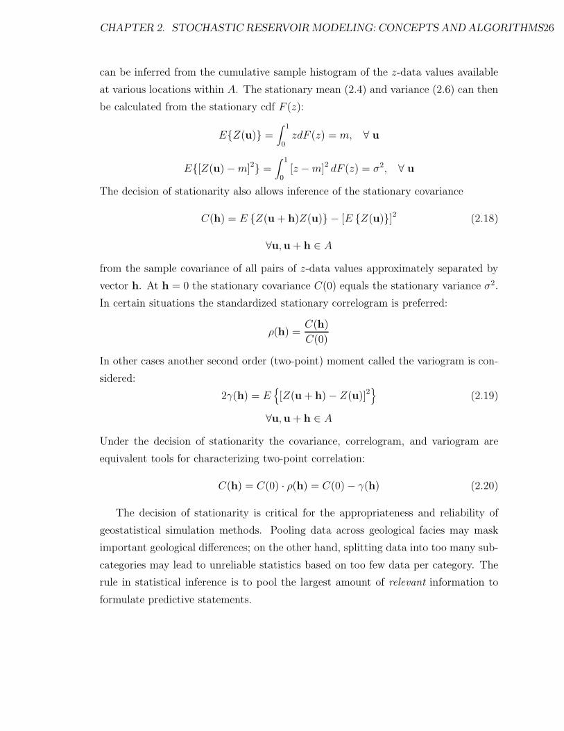
CHAPTER 2. STOCHASTIC RESERVOIR MODELING: CONCEPTS AND ALGORITHMS26
can be inferred from the cumulative sample histogram of the z-data values available
at various locations within A. The stationary mean (2.4) and variance (2.6) can then
be calculated from the stationary cdf F (z):
E{Z(u)} =∫ 1
0zdF (z) = m, ∀ u
E{[Z(u) − m]2} =∫ 1
0[z − m]2 dF (z) = σ2, ∀ u
The decision of stationarity also allows inference of the stationary covariance
C(h) = E {Z(u + h)Z(u)} − [E {Z(u)}]2 (2.18)
∀u,u + h ∈ A
from the sample covariance of all pairs of z-data values approximately separated by
vector h. At h = 0 the stationary covariance C(0) equals the stationary variance σ2.
In certain situations the standardized stationary correlogram is preferred:
ρ(h) =C(h)
C(0)
In other cases another second order (two-point) moment called the variogram is con-
sidered:
2γ(h) = E{[Z(u + h) − Z(u)]2
}(2.19)
∀u,u + h ∈ A
Under the decision of stationarity the covariance, correlogram, and variogram are
equivalent tools for characterizing two-point correlation:
C(h) = C(0) · ρ(h) = C(0) − γ(h) (2.20)
The decision of stationarity is critical for the appropriateness and reliability of
geostatistical simulation methods. Pooling data across geological facies may mask
important geological differences; on the other hand, splitting data into too many sub-
categories may lead to unreliable statistics based on too few data per category. The
rule in statistical inference is to pool the largest amount of relevant information to
formulate predictive statements.

CHAPTER 2. STOCHASTIC RESERVOIR MODELING: CONCEPTS AND ALGORITHMS27
Stationarity is a property of the RF model; thus, the decision of stationarity may
change if the scale of the study changes or if more data become available. If the goal
of the study is global then local details may be unimportant; conversely, the more
data available the more statistically significant differentiations become possible.
2.3.3 Kriging
Kriging was initially introduced to provide estimates for unsampled values z(u).
Within the context of stochastic simulation, however, it is used to build probabilistic
models of uncertainty about these unknown values (see (2.2) and Lesson 4 in [83]).
Essentially, the kriging algorithm provides a minimum error variance estimate of any
unsampled value based on a stationary two-point covariance (2.18). Contouring a
grid of kriging estimates is the traditional mapping application of kriging. However,
since kriging estimates are weighted moving averages of the data, their distribution
smooths out details and extreme values of the original data set. Thus, it is not an
appropriate algorithm to generate input numerical models for flow simulation since
the extreme permeability values, i.e., flow paths and barriers are critical to the fluid
flow response [63].
The minimum error variance property of kriging allows it to approximate, and
in some cases identify, the conditional expectation of the variable being estimated.
Thus, kriging can be used to determine a series of posterior conditional probability
distributions from which stochastic images of the attribute spatial distribution can
be drawn. This aspect of kriging which is key to the random function approach
to stochastic simulation, will be discussed in the next section. The following is a
summary of kriging. More details and theoretical proofs can be found in [22, 29, 54,
65, 69, 83, 90, 98].
All versions of kriging are elaborations on the same basic linear regression algo-
rithm and corresponding estimator:
[Z∗SK(u) − m(u)] =
n∑α=1
λα(u) [Z(uα) − m(uα)] (2.21)
where Z(u) is the RV model at location u, the uα’s are the n data locations, m(u)

CHAPTER 2. STOCHASTIC RESERVOIR MODELING: CONCEPTS AND ALGORITHMS28
= E{Z(u)} is the expected value of RV Z(u), and Z∗SK(u) is the linear regression
estimator, also called the “simple kriging” (SK) estimator.
The SK weights λα(u) are given by the system of normal equations written in
their general non-stationary form as follows:
n∑β=1
λβ(u)C(uβ,uα) = C(u,uα), α = 1, . . . , n (2.22)
The SK algorithm requires prior knowledge of the (n+1) means m(u), m(uα), α =
1, . . . , n , and the (n + 1) by (n + 1) covariance matrix [C(uα,uβ), α, β = 0, 1, . . . , n]
with u0 = u. In most practical situations, inference of these means and covariance
values requires a prior decision of stationarity of the random function Z(u) (see the
discussion in the previous section). If the RF Z(u) is stationary with constant mean
m, and covariance function C(h) = C(u,u + h), ∀u, the SK estimator reduces to its
stationary version:
Z∗SK(u) =
n∑α=1
λα(u)Z(uα) +
[1 −
n∑α=1
λα(u)
]m (2.23)
where the weights λα(u) are established to minimize the error variance or estimation
variance:
σ2E(u) = E
{[Z(u) − Z∗
SK(u)]2}
(2.24)
Solution of the traditional stationary SK system:
n∑β=1
λβ(u)C(uβ − uα) = C(u− uα), α = 1, . . . , n (2.25)
provides the weights λα(u) such that the estimator (2.23) minimizes the estimation
variance (2.24). The minimized estimation variance or kriging variance is given by:
σ2SK(u) = C(0) −
n∑α=1
λα(u)C(u − uα) (2.26)
where, C(0) is the stationary variance σ2.
According to strict stationary theory, SK is the algorithm that should be applied;
however, stationary SK does not adapt to local trends in the data since it relies on the
mean value m assumed known and constant throughout the area. Consequently, when

CHAPTER 2. STOCHASTIC RESERVOIR MODELING: CONCEPTS AND ALGORITHMS29
enough data are available to identify trends, the more robust ordinary kriging (OK)
algorithm is used. Ordinary kriging (OK) filters the mean from the SK estimator
(2.23) by requiring that the kriging weights sum to one. This results in the following
ordinary kriging (OK) estimator:
Z∗OK(u) =
n∑α=1
να(u)Z(uα) (2.27)
and the stationary OK system:
∑n
β=1 νβ(u)C(uβ − uα) + µ(u) = C(u − uα), α = 1, . . . , n∑nβ=1 νβ(u) = 1
(2.28)
where the να(u)’s are the OK weights and µ(u) is the Lagrange parameter associated
to the constraint∑n
β=1 νβ(u) = 1. Comparing expression (2.25) and (2.28), note that
the SK weights are different from the OK weights.
2.3.4 Models of Uncertainty
At the beginning of the previous section it was noted that the primary usefulness of
kriging, in the context of stochastic simulation, is in the determination of posterior
distribution models. There are two characteristic properties of kriging that are the
basis for, respectively, the multiGaussian (MG) approach and the indicator kriging
(IK) approach to the determination of posterior ccdf’s:
(i) - The multiGaussian Approach: If the RF model Z(u) is multivariate nor-
mal or Gaussian5, then the simple kriging estimate (2.23) and variance (2.26)
identify the mean and variance of the posterior ccdf. In addition, since that
ccdf is Gaussian, it is fully determined by these two parameters, see [9] and
[134]. This rather simple result is the basis for multiGaussian (MG) kriging
and simulation. The MG approach is said to be parametric in the sense that it
determines the ccdf’s through their parameters (mean and variance).
5Since one cannot expect all sample histograms to be normal, a normal score-transform is per-formed on the original z-data. A multiGaussian model Y (u) is then adopted for the normal scoredata. Kriging and simulation are performed on the y-data with the results appropriately back-transformed into z-values.
CHAPTER 2. STOCHASTIC RESERVOIR MODELING: CONCEPTS AND ALGORITHMS30
(ii) - The Indicator Kriging Approach: If the value to be estimated is the ex-
pected value (mean) of a distribution, then least squares (LS) regression, i.e.,
kriging, is a priori the preferred algorithm. The reason is that the LS estimator
of the variable Z(u) is also its conditional expectation E{Z(u)|(n)}, i.e., the
mean of the ccdf (2.2) (see [90], p. 566). Now, instead of the variable Z(u), con-
sider its binary indicator transform I(u; z) as defined in relation (2.11). Kriging
of the indicator RV I(u; z) provides an estimate which is also the LS estimate
of the conditional expectation of I(u; z). Moreover, the conditional expectation
of I(u; z) is itself equal to the ccdf of Z(u); indeed:
E {I(u; z)|(n)} = 1 · Prob {I(u; z) = 1|(n)}+ 0 · Prob {I(u; z) = 0|(n)}
= 1 · Prob {Z(u) ≤ z)|(n)} ≡ F (u; z|(n)), as defined in (2.2)
Thus, the kriging algorithm applied to indicator data provides LS estimates of
the ccdf (2.2). Note that indicator kriging (IK) is not aimed at estimating the
unsampled value z(u) or its indicator transform i(u; z) but at providing a ccdf
model of uncertainty about z(u). The IK algorithm is said to be non-parametric
in the sense that it does not approach the ccdf through its parameters, rather,
the ccdf values for various threshold values z are estimated directly.
Given these two algorithms for updating prior models of uncertainty (2.1) to
posterior models of uncertainty (2.2) it is possible to discuss an important family of
stochastic simulation techniques.
2.3.5 The Sequential Approach to Stochastic Simulation
Consider a random function (RF) defined over some field of interest, e.g.,
{Z(u),u ∈ study area A}
Stochastic simulation is the process of building alternate, equally probable models
of the spatial distribution of z(u); each realization is denoted with the superscript l:

CHAPTER 2. STOCHASTIC RESERVOIR MODELING: CONCEPTS AND ALGORITHMS31
{z(l)(u),u ∈ A}. The simulation is said to be “conditional” if the resulting realizations
honor the hard data values at their locations:
z(l)(uα) = z(uα), ∀ l, α = 1, . . . , n (2.29)
The simulated realizations are built such that they honor aspects of the multivariate
probability distribution of the RF chosen to model Z(u). In all cases, except for the
multiGaussian RF model, those aspects of the multivariate distribution are limited
to moments of its bivariate distribution.
Consider the joint distribution of N random variables Zi with N very large. The
N RV’s Zi may represent a single attribute, say permeability, at the N nodes of a
dense grid discretizing the field A, or they can represent N attributes measured at
the same location, or they could represent a combination of K different attributes
defined at the N ′ nodes of a grid with N = KN ′.
Next, consider the conditioning of these N RV’s by a set of n data of any type
symbolized by the notation |(n). The corresponding N -variate ccdf is denoted:
F(N)(z1, . . . , zN |(n)) = Prob{Zi ≤ zi, i = 1, . . . , N |(n)} (2.30)
Expression (2.30) is completely general with no intrinsic limitations; some or all of
the variables Zi could be categorical.
Successive application of Bayes’ relation shows that drawing an N -variate sample
from the ccdf (2.30) can be done in N successive steps, each involving a univariate
ccdf with increasing levels of conditioning:
• draw a value z(l)1 from the univariate ccdf of Z1 given the original data (n). The
value z(l)1 is now considered as a conditioning datum for all subsequent drawings;
thus, the information set (n) is updated to (n + 1) = (n) ∪ {Z1 = z(l)1 }.
• draw a value z(l)2 from the univariate ccdf of Z2 given the updated data set
(n + 1), then update the information set to (n + 2) = (n + 1) ∪ {Z2 = z(l)2 }.
• sequentially consider all N RV’s Zi.

CHAPTER 2. STOCHASTIC RESERVOIR MODELING: CONCEPTS AND ALGORITHMS32
The set {z(l)i , i = 1, . . . , N} represents a simulated joint realization of the N dependent
RV’s Zi. If another realization is needed, {z(l′)i , i = 1, . . . , N}, the entire sequential
drawing process is repeated.
This sequential simulation procedure requires the determination of N univariate
ccdf’s, more precisely:
Prob{Z1 ≤ z1|(n)} (2.31)
Prob{Z2 ≤ z2|(n + 1)}Prob{Z3 ≤ z3|(n + 2)}
. . .
P rob{ZN ≤ zN |(n + N − 1)}
The sequential simulation principle is the same regardless of the algorithm or model
used to establish the sequence (2.31) of univariate ccdf’s. In the multiGaussian ap-
proach all ccdf’s (2.31) are assumed Gaussian and their means and variances are
given by a series of N simple kriging systems (see the previous section 2.3.4). In the
indicator kriging approach, the ccdf’s are obtained directly by indicator kriging (see
the previous section 2.3.4).
Implementation Considerations:
• Strict application of the sequential simulation principle calls for the determina-
tion of more and more complex ccdfs, in the sense that the size of the condi-
tioning data set increases from (n) to (n + N − 1). In practice, the argument is
that the closer6 data screens the influence of more remote data; therefore, only
the closest data are retained to condition any of the N ccdfs (2.31).
• The neighborhood limitation of the conditioning data entails that statistical
properties of the (N +n) set of RV’s will be reproduced only up to the maximum
distance found in the neighborhood7. For example, the search must be at least
6“Closer” is not necessarily taken in terms of Euclidean distance, particularly if the original dataset (n) and the N RV’s include different attribute values. The data “closest” to each particular RVZi being simulated are those that have the most influence on its ccdf.
7Larger scale conditioning could be imparted from local conditioning data [99]

CHAPTER 2. STOCHASTIC RESERVOIR MODELING: CONCEPTS AND ALGORITHMS33
as large as the distance to which the covariance is to be reproduced; this requires
extensive conditioning as the sequence progresses from 1 to N . One solution
is provided by the multiple grid concept which is to simulate the N nodal
values in two or more steps [55]: First, a coarse grid, say every tenth node is
simulated using a large data neighborhood. The large neighborhood allows the
reproduction of large scale covariance structures. Second, the remaining nodes
are simulated with a smaller neighborhood.
• Theory does not specify the sequence in which the N nodes should be simulated;
practice has shown that it is better to use a random sequence [68].
2.3.6 Sequential Gaussian Simulation (SGS)
The most straightforward algorithm for generating realizations of a multivariate Gaus-
sian field is provided by the sequential principle described above. Each variable is
simulated sequentially according to its normal ccdf fully characterized through a SK
system of type (2.25). The conditioning data consist of all original data and all previ-
ously simulated values found within a neighborhood of the location being simulated.
The conditional simulation of a continuous variable z(u) modeled by a Gaussian-
related stationary RF Z(u) proceeds as follows:
1. Determine the univariate cdf FZ(z) representative of the entire study area and
not only of the available z-data. Declustering may be needed if the z-data are
preferentially located [37, 40, 77].
2. Perform the normal score transform of the z-data, with the FZ(z) cdf, into
y-data with a standard normal cdf [40, 90].
3. Although not a part of the algorithm, it is good practice to check for bivariate
normality of the normal score y-data by comparing the experimental indicator
variograms to the ones expected from multiGaussian theory (see [40, 138]). If
the data do not show a bivariate Gaussian behavior, then alternate models
such as a mixture of Gaussian populations [141] or an indicator-based approach
should be considered.

CHAPTER 2. STOCHASTIC RESERVOIR MODELING: CONCEPTS AND ALGORITHMS34
4. If a multivariate Gaussian RF model is adopted for the y-variable then proceed
with sequential simulation, i.e.,
• define a random path that visits each node of the grid (not necessarily
regular) once. At each node u, retain a specified number of neighboring
conditioning data including both original y data and previously simulated
grid node y-values.
• use SK to determine the parameters (mean and variance) of the ccdf of
the RF Y (u) at location u.
• draw a simulated value y(l)(u) from that ccdf
• add the simulated value y(l)(u) to the data set
• proceed to the next node, and loop until all nodes are simulated.
5. Backtransform the simulated normal values {y(l)(u),u ∈ A} into simulated
values for the original variable {z(l)(u) = ϕ−1(y(l)(u)),u ∈ A}. Within-class
interpolations and tail extrapolations are usually called for, see [40] for details.
If multiple realizations are desired {z(l)(u),u ∈ A}, l = 1, . . . , L, the previous
algorithm is repeated L times with a different random path for each realization.
The prior decision of stationarity requires that simple kriging (SK) with zero mean
(for Y (u)) be used in step 4 of the SGS algorithm. However, if there are enough data
to indicate that a non-stationary RF model would be more appropriate, one may
• either split the area into distinct sub-zones and consider for each sub-zone a dif-
ferent RF model, which implies inference of a different normal score covariance
for each sub-zone,
• or consider a stationary normal score covariance, inferred from the entire pool of
data, and a non-stationary mean for Y (u). The non-stationary mean, E{Y (u)},at each location u, is implicitly re-estimated from the neighborhood data through
ordinary kriging (OK), see section 2.3.3. Locally rescaling the model mean usu-
ally results in a poorer reproduction of the stationary Y -covariance model.

CHAPTER 2. STOCHASTIC RESERVOIR MODELING: CONCEPTS AND ALGORITHMS35
A number of implementations of the sequential Gaussian simulation (SGS) algo-
rithm exist. The program gsim3d.c written by Isaaks [68] and the sgsim program of
GSLIB [40] are two published versions.
2.3.7 Sequential Indicator Simulation (SIS)
Rather than adopt a multiGaussian RF model one could consider a non-parametric
indicator kriging approach as described in section 2.3.4. For details and the theoretical
development of the sequential indicator simulation methodology see [8, 55, 83, 89,
115]. In this approach, kriging is applied to binary indicator transforms of the data
to directly estimate conditional probabilities:
• if the indicator variable being kriged arises from a categorical variable, i.e., i(u)
set to 1 if the location u belongs to category k, to zero otherwise, then:
Prob{I(u) = 1|(n)} = E{I(u)|(n)} (2.32)
• if the variable z(u) to be simulated is continuous, its ccdf can also be written
as an indicator conditional expectation:
Prob{Z(u) ≤ z|(n)} = E{I(u; z)|(n)} (2.33)
with I(u; z) = 1 if Z(u) ≤ z, =0 otherwise.
In both cases, the problem of evaluating the conditional probability is mapped
onto that of evaluating the conditional expectation of a specific indicator RV. The
evaluation of a conditional expectation calls for well-established regression theory,
i.e., kriging (see section 2.3.3).
The sequential simulation algorithm proceeds somewhat differently for categorical
and continuous variables:
(i) - Categorical Variables: At each node u along the random path, indicator krig-
ing followed by order relation corrections8 provides K estimated probabilities
8Order relation corrections amount to ensuring that the estimated distribution follows the axiomsof a probability distribution: a cdf is never less than 0, greater than 1, and must be non-decreasing.The probabilities of a pdf must all be greater (or equal to) zero and sum to one.

CHAPTER 2. STOCHASTIC RESERVOIR MODELING: CONCEPTS AND ALGORITHMS36
p∗k(u|(·)). The conditioning information (·) consists of both the original ik-data
and the previously simulated ik-values for category k.
Next define any ordering of the K categories, say 1,2,. . . ,K. This ordering
defines a cdf-type scaling of the probability interval [0, 1] with K intervals, say:
[0, p∗1(·)], (p∗1(·), p∗2(·) + p∗1(·)], . . . , (1 −K−1∑k=1
p∗k(·), 1]
Draw a random number p uniformly distributed in [0, 1]. The interval in which
p falls determines the simulated category at location u.
Update all K indicator data sets with this new simulated information, and
proceed to the next location u′ along the random path.
The arbitrary ordering of the K probabilities p∗k(·) does not affect which category
is drawn nor the spatial distribution of categories [8].
(ii) - Continuous Variables: The continuous variable z(u) discretized into K mu-
tually exclusive classes k : (zk−1, zk], k = 1, . . . , K can be interpreted and simu-
lated as the spatial distribution of K class indicators.
One advantage of considering the continuous variable z(u) as a paving (mosaic)
of K classes is the flexibility to model the spatial distribution of each class by a
different indicator covariance. For example, in the absence of any facies infor-
mation, the class of highest permeability corresponding to a complex network of
fractures, may be modeled by a zonal anisotropic indicator covariance with the
maximum direction of continuity in the fracture direction; while the geometry
of the classes of low-to-median permeability values could be modeled by more
isotropic indicator covariances. The indicator formalism allows for modeling
mixtures of populations loosely9 defined as classes of values of a continuous
attribute z(u) [30, 80].
9Note that major heterogeneities characterized by actual categorical variables, such as lithofaciestypes, should be dealt with (simulated) first, e.g., through categorical indicator simulation or consid-ering a Boolean process (the simulation of objects with a predefined shape). However, there are casesand/or scales where the only property recorded is a continuous variable such as a porosity value oracoustic log; yet experience tells us that this continuous variable is measured across heterogeneouspopulations. In this case the indicator formalism allows a “loose” separation of populations throughdiscretization of the range of the continuous attribute measured [80].

CHAPTER 2. STOCHASTIC RESERVOIR MODELING: CONCEPTS AND ALGORITHMS37
At each node u to be simulated along the random path indicator kriging (SK
or OK) provides a ccdf through K probability estimates:
F ∗(u; zk|(n)) = Prob∗{Z(u) ≤ z|(n)}, k = 1, . . . , K
Within-class interpolation, see [40], provides the continuum for all threshold
values z ∈ [zmin, zmax].
Monte-Carlo simulation of a realization z(l)(u) is obtained by drawing a uniform
random number p(l) ∈ [0, 1] and retrieving the ccdf p(l)-quantile:
z(l)(u) = F ∗−1(u; p(l)|(n)) (2.34)
such that : F ∗(u; z(l)(u)|(n)) = p(l)
The indicator data set (for all cutoffs zk) is updated with the simulated value
z(l)(u), and indicator kriging is performed at the next location u′ along the
random path.
Once all locations u have been simulated, a stochastic image {z(l)(u), u ∈ A} is
obtained. The entire sequential simulation process with a new random path can be
repeated to obtain another independent realization {z(l′)(u),u ∈ A}, l′ �= l.
The indicator approach is well suited to categorical variables which are naturally
expressed as binary indicators. The indicator approach is not as natural for continuous
variables because of the need for within class interpolations. However, there are a
number of advantages of the indicator formalism:
• The major advantage of the indicator kriging approach to generating posterior
conditional distributions (ccdf’s) is its ability to account for soft data. As long as
the soft or fuzzy data can be coded into prior local probability values, indicator
kriging can be used to integrate that information into a posterior probability
value [6, 45, 81, 92].
The prior information can take one of the following forms:
– local hard indicator data i(uα; z) originating from local hard data z(uα):
i(uα; z) = 1 if z(uα) ≤ z, = 0 if not (2.35)

CHAPTER 2. STOCHASTIC RESERVOIR MODELING: CONCEPTS AND ALGORITHMS38
or ik(uα) = 1 if uα ∈ category k, = 0 if not
– local hard indicator data j(uα; z) originating from ancillary information
that provides hard inequality constraints on the local value z(uα). If
z(uα) ∈ (aα, bα], then:
j(uα; z) =
0 if z ≤ aα
undefined (missing) if z ∈ (aα, bα]
1 if z > bα
(2.36)
– local soft indicator data y(uα; z) originating from ancillary information
providing prior (pre-posterior) probabilities about the value z(uα):
y(uα; z) = Prob{Z(uα) ≤ z| local information} (2.37)
∈ [0, 1]
�= F (z) : global prior as defined below
However, usually E{Y (u; z)} = F (z).
– global prior information common to all locations u within the stationary
area A:
F (z) = Prob{Z(u) ≤ z}, ∀ u ∈ A (2.38)
At any location u ∈ A, prior information about the value z(u) is characterized
by any one of the four previous prior probability distributions. The IK process
consists of a Bayesian updating of the local prior cdf into a posterior cdf using
information supplied by neighboring local prior cdf’s [17, 92, 140].
• A second major advantage of the indicator formalism over most other ap-
proaches to estimation and simulation is the possibility of accounting for soft
structural information. That is, the bivariate distribution can be more fully
specified by data rather than summarized by a single covariance. Inferring
different indicator covariance models at each threshold value allows a better
representation of the spatial correlation; however, the ability to incorporate
soft information may be retained while only retaining one indicator covariance
(see the median IK approach documented below).

CHAPTER 2. STOCHASTIC RESERVOIR MODELING: CONCEPTS AND ALGORITHMS39
The Median IK Approach
In indicator kriging the K cutoff values zk are usually chosen so that the corresponding
indicator covariances CI(h; zk) are different from one another. However, there are
cases when the sample indicator covariances/variograms appear proportional to each
other, i.e., the sample indicator correlograms are all similar. The corresponding
continuous RF model Z(u) is the so-called “mosaic” model [79] such that:
ρZ(h) = ρI(h; zk) = ρI(h; zk; zk′), ∀zk, zk′ (2.39)
where ρZ(h) and ρI(h; zk) are the correlograms and cross-correlograms of the contin-
uous RF Z(u) and its indicator transforms.
Then, the single correlogram function is better estimated either directly from the
sample Z-correlogram or from the sample indicator correlogram at the median cutoff
zk = M , such that F (M) = 0.5. Indeed, at the median cutoff, the indicator data are
evenly distributed as 0 and 1 values with, by definition, no extreme values.
Indicator kriging under the model (2.39) is called “median indicator kriging” [77].
It is a particularly simple and fast procedure since it calls for a single easy-to-infer
median indicator variogram which is used for all K cutoffs. Moreover, if the indicator
data configuration is the same for all cutoffs10, one single IK system needs to be solved
with the resulting weights being used for all cutoffs.
The median IK algorithm applied in conjunction with sequential indicator simu-
lation is used extensively in later chapters.
2.4 Geological Structures and Well Test Data
The sequential Gaussian simulation (SGS) and sequential indicator simulation (SIS)
algorithms are state-of-the-art simulation methods [55, 56, 68, 86, 85] that have con-
tributed significantly to reservoir modeling and risk-qualified decision making. Nev-
ertheless, these methods and all their enhancements [92, 128, 140] are limited to cases
10Unless inequality constraint-type data z(uα) ∈ (aα, bα] are considered, the indicator data con-figuration is the same for all cutoffs zk’s as long as the same data locations uα’s are retained for allcutoffs.

CHAPTER 2. STOCHASTIC RESERVOIR MODELING: CONCEPTS AND ALGORITHMS40
when the spatial continuity is characterized by stationary two-point statistics and to
data that is defined on the same support11.
This section documents two important cases when conventional geostatistical tech-
niques fail to account for important prior information:
1. Most common geological structures have curvilinear directions of continuity
and multiple-point connectivity that are difficult to account for with the con-
ventional RF “covariance-based” techniques. In many cases this information is
crucial to yield geologically realistic stochastic models of reservoir properties.
2. Pressure transient well testing provides critical information about the reservoir
properties at a significantly larger scale than can be measured by core or well
logging tools. Specifically, the average absolute permeability inferred from a
well test constrains the spatial distribution of permeability near the well bore,
i.e., the stochastic reservoir models.
The next two sections (2.4.1 and 2.4.2) illustrate these types of data and show the
inadequacy of conventional stochastic simulation techniques.
2.4.1 Geological Structures
Conventional stochastic simulation methods rely on a prior decision of stationarity
and two-point covariance functions C(h) to describe the spatial correlation within
each stationary zone A. The decision of stationarity implies that the major direc-
tion of continuity is the same throughout A, recall the definition of the stationarity
covariance (2.18):
C(h) = E {Z(u + h)Z(u)} − [E {Z(u)}]2 (2.40)
∀u,u + h ∈ A
Thus, the specific locations of two points separated by h is not information retained
in the stationary covariance (2.40). Any curvilinear patterns of continuity, or the
11Data of different supports may only be considered if the averaging is linear which is not the casefor permeability.

CHAPTER 2. STOCHASTIC RESERVOIR MODELING: CONCEPTS AND ALGORITHMS41
presence of subregions with different directions of continuity, within the stationary
zone A are represented with an average covariance showing only the average direction
of continuity12.
For example, a cross section through an eolian sandstone is shown on the top
of Figure 2.4 (Appendix A documents the procedure used to acquire the geological
images used as examples here and in later chapters). The simulated realization,
generated with the sequential Gaussian simulation (see section 2.3.6), reproduces the
two-point indicator covariances; however, the curvilinear features are not reproduced
due to the decision of stationarity and the restriction to two-point statistics.
A second example of cross stratified sands and silty sands from a distributary bar
deltaic environment is shown on Figure 2.5. The simulated realization was created by
a full indicator simulation (see section 2.3.7) with seven cutoffs (at all the seven gray
scale thresholds). Once again, the multiple-point connectedness and the curvilinear
features are not characterized by stationary two-point statistics.
As a last example, consider the two control patterns shown at the top of Figure 2.6;
both are the result of Boolean simulations whereby predefined shapes are located at
random. The left control pattern shows linear structures and the right image shows
curvilinear structures. All stationary two-point histograms were retained for 25 lags
in 2 directions and used to condition two simulations of each control pattern (the
methodology to accomplish this will be discussed in section 2.5 and in later chapters).
The two inadequacies of stationary two-point statistics are illustrated by this simple
example:
1. The reproduction of the linear control pattern is quite good. The anisotropy is
well characterized; however, the fact that all of the anisotropic dark gray rect-
angles have exactly an 8:1 anisotropy (i.e., the rectangles were all constructed
1 unit thick and 8 units long) is not captured by two-point statistics. Multiple
point connectivity, even if linear, is not captured by two-point statistics.
2. The reproduction of the curvilinear control pattern is poor. Stationary two-
point statistics are inadequate for capturing any continuity that is not linear;
12In certain cases it is possible to consider curvilinear coordinate systems to avoid the problemsintroduced by a single stationary zone [28, 41, 121].

CHAPTER 2. STOCHASTIC RESERVOIR MODELING: CONCEPTS AND ALGORITHMS42
Eolian Sandstone Image
Gaussian Simulation
Figure 2.4: The upper image shows a cross section through an eolian sandstone. The lowerimage was created by Gaussian simulation (see section 2.3.6) with the exhaustive normalscores variogram of the upper image.

CHAPTER 2. STOCHASTIC RESERVOIR MODELING: CONCEPTS AND ALGORITHMS43
Cross Stratified Sands and Silty Sands
Indicator Simulation
Figure 2.5: The upper image shows an image of cross stratified sands and silty sands.The lower image was created with two-point information in the form of complete indicatorvariogram models (see the sequential indicator simulation described in section 2.3.7.

CHAPTER 2. STOCHASTIC RESERVOIR MODELING: CONCEPTS AND ALGORITHMS44
at least trivariate statistics are required for curvilinear features.
In certain cases, non-linear features are essential for a realistic representation
of the spatial distribution. There are two evident ways that information on these
features could be accounted for: 1) the decision of stationarity could be relaxed
by separating the stationary area A into subzones each with different directions of
continuity [41, 121], and 2) multiple-point statistics could be considered to more fully
describe the multivariate distribution of Z(u) within A.
Relaxing the decision of stationarity to make up for the inadequacy of two-point
statistics has been somewhat successful when locally stationary subregions can be
established. Many geological features are non-linear even at a small scale which
implies that the subregions will be too small to allow inference of the needed statistics
or anisotropy directions. In this case, multiple-point statistics are called for to more
completely define the multivariate distribution.
A Comment on Exhaustive Two Point Statistics
It can be shown that exhaustive bivariate (two point) statistics contain enough in-
formation to reproduce a finite image exactly [49]. This is interesting but inconse-
quential; in fact, without assuming stationarity univariate statistics also allow exact
reproduction of an image13.
The reproduction of an image with bivariate statistics is possible because the
outermost points are established first, then the second outermost, . . . , until the central
point is finally established. In stochastic simulation, the point is not to reproduce
exactly the training image but to extract its essence with limited statistics.
Bivariate statistics available for every possible lag vector h over a specific areal
extent B, smaller than the training image A, do not necessarily capture the features
smaller than B. For example, if there were curvilinear features smaller than B or
there was a multiple-point connectivity, still less than B, then exhaustive two-point
statistics for all vectors h ∈ B are not sufficient. For example, consider the training
image on the left of Figure 2.7 where the circular shapes are less than four pixels in
13The histogram at each location is exactly the value specified by the training image. The valuesare not pooled into a histogram representative of a larger volume.

CHAPTER 2. STOCHASTIC RESERVOIR MODELING: CONCEPTS AND ALGORITHMS45
Linear Control Pattern Curvilinear Control Pattern
Simulation One Simulation One
Simulation Two Simulation Two
Figure 2.6: An example of a linear structure, well characterized by bivariate statistics,and a curvilinear structure, poorly characterized by bivariate statistics. Two simulationsof each are shown below the control patterns. All four simulations reproduce the two pointstatistics for 20 lags in two directions.

CHAPTER 2. STOCHASTIC RESERVOIR MODELING: CONCEPTS AND ALGORITHMS46
Curvilinear Training Image
Subarea B forControl Statistics
Simulated Realization
Figure 2.7: A curvilinear training image, the areal extent of exhaustive two-point statistics,and a simulated realization honoring the two-point statistics.
diameter. Reproducing all two point statistics for a subarea B four by four pixels
does not reproduce the circular shapes.
There is a need for simulation techniques that could directly account for multiple-
point statistics and, indirectly, the curvilinear features described above. There is also
a need for techniques to create realizations conditional to information available at a
significantly larger scale, e.g., that measured by pressure transient well testing.
2.4.2 Well Test Data
A pressure transient well test is conducted by altering the production conditions
(flow rate) and monitoring the reservoir pressure response [66]. Different reservoir
properties may be interpreted from the pressure response:
• The effective permeability or conductivity (permeability-thickness product) near
the well is an important parameter needed to predict future performance and
design well spacing.
• The reservoir pressure which is needed to predict the in-situ resource and an
appropriate recovery scheme for future exploitation.
• In many cases the reservoir limits may be predicted. These limits are essential

CHAPTER 2. STOCHASTIC RESERVOIR MODELING: CONCEPTS AND ALGORITHMS47
to establish the in-situ resource.
• In some cases it is possible to identify the presence of faults, fluid fronts, strati-
graphic interfaces, and other barriers.
The latter three pieces of information typically enter the reservoir model determin-
istically. That is, the reservoir pressure, limits, and major faults are all directly ac-
counted for in the stochastic models or when setting up the flow simulator. The first
piece of information, which informs the spatial distribution of absolute permeability,
could be used directly in a homogeneous or layer-cake reservoir model14. However,
it can not be accounted for by any conventional geostatistical/statistical technique
that constructs heterogeneous models (see section 2.2) of the reservoir properties (in
particular permeability).
The permeability inferred from a well test carries important information because
all other measurements are on a scale many orders of magnitude smaller than the
grid blocks typically used in flow simulators. It could be argued that well test, or
engineering data in general, are the most important because they are intimately
related to the recovery process and the response variables that will form the basis for
reservoir management decisions.
For example, an actual well test provides a single true effective permeability near
the well at which the test was conducted. If the same well test is numerically simulated
on stochastic models, that are conditional only to core measurements and the global
histogram of permeability values, the test results may not match the single known
permeability value. This is illustrated by the histogram of well test-derived effective
permeability values which is shown on Figure 2.8. These values were all derived
by numerically simulating a well test on 100 multiGaussian simulated realizations
that honored the permeability at the well location, the univariate distribution, and
the stationary covariance C(h) of the permeability values (the details of this study
are given in chapter 3). Ideally, if all the information were accounted for, the 100
simulated values should be all equal to the single value inferred from the well test
performed in the field (1.73 md).
14The permeanbility of the homogeneous model or the appropriate layers could be set equal tothe well test-derived value.

CHAPTER 2. STOCHASTIC RESERVOIR MODELING: CONCEPTS AND ALGORITHMS48
Fre
quen
cy
Well Test-Derived Permeability, md
.00 1.00 2.00 3.00 4.00 5.00 6.00 7.00
.000
.040
.080
.120
mean 2.56std. dev. 1.12
coef. of var .44
maximum 6.44upper quartile 3.43
median 2.25lower quartile 1.79
minimum .52
Figure 2.8: The distribution of permeability derived from well tests performed on 100stochastic reservoir models.
2.5 Annealing Techniques for Stochastic Simula-
tion
In the “annealing” approach to stochastic simulation there is no explicit random
function model, rather, the creation of a simulated realization is formulated as an
optimization problem to be solved with a stochastic relaxation or “annealing” tech-
nique. The first requirement of this class of methods is an objective (or energy)
function which is some measure of difference between the desired spatial characteris-
tics and those of a candidate realization. The essential feature of stochastic relaxation
methods is to perturb iteratively (relax) the candidate realization and then accept or
reject the perturbation with some decision rule. The decision rule is based on how
much the perturbation has brought the candidate image closer to having the desired
properties. One possible decision rule is based on an analogy with the physical process
of annealing, hence the name simulated annealing15. Annealing is the process where
15Technically the name “simulated annealing” applies only to those stochastic relaxation methodsbased strictly on simulated annealing [1, 93]; however, through common usage the name “anneal-ing” is used to describe the entire family of methods that are based on the principle of stochastic

CHAPTER 2. STOCHASTIC RESERVOIR MODELING: CONCEPTS AND ALGORITHMS49
a metallic alloy is heated without leaving the solid phase so that molecules may move
positions relative to one another and reorder themselves into a low energy crystal (or
grain) structure. The probability that any two molecules will swap locations is known
to follow the Boltzmann distribution. Simulated annealing is the application of the
annealing mechanism of perturbation and the Boltzmann probability distribution for
accepting perturbations.
At first glance this approach appears terribly inefficient. For example, if every
nodal value z(l)(ui), i = 1, . . . , N in the candidate image is initially assigned by ran-
domly drawing from the stationary cdf F (z) then millions of perturbations may be
required to arrive at an image that has the desired spatial structure. In practice,
these methods are more efficient than they might seem since remarkably few arith-
metic operations are required to update the objective function after a perturbation;
virtually all conventional global spatial statistics (e.g., a covariance) may be updated
locally rather than globally recalculated after a local perturbation. The real interest
in annealing techniques stems from a hope that they will be able to integrate better
complex geological structures and engineering data. .
The conventional stochastic simulation techniques documented in section 2.3 are
limited to two-point statistics. Annealing is not limited to two-point statistics. The
objective function is defined as some measure of difference between a set of reference
properties and the corresponding properties of a candidate realization. The refer-
ence properties could consist of any quantified geological, statistical, or engineering
property.
In many applications the reference properties/statistics are derived from a full
valued array of values referred to as a training image or control pattern. The concept
is that these training images will come from outcrop mapping, zones with a significant
amount of conditioning data, or perhaps from the output of programs that simulate
geological processes from first principles [131]. An advantage of using a training image
is that the reference statistics are, by definition, consistent in that there exists at least
one realization that reproduces them all. If a suitable training image is unavailable
the reference statistics may be inferred from sparsely sampled data or analog data.
relaxation.

CHAPTER 2. STOCHASTIC RESERVOIR MODELING: CONCEPTS AND ALGORITHMS50
Annealing does not require a training image; the method requires reference properties
or statistics regardless of their origin.
To illustrate the application of the annealing methodology, consider a categorical
variable Z(u) that can take any one of K outcome values k = 1, . . . , K. The stochastic
simulation problem considered here is to generate a spatial distribution for Z(u) at N
grid node locations: z(ui), i = 1, . . . , N . To be useful each simulated realization must
share certain spatial statistics with those inferred from actual data. As an example
statistic, consider the stationary16 two-point histogram, see also (2.13):
f(h; k1, k2) = Prob {Z(u) ∈ category k1, Z(u + h) ∈ category k2, } (2.41)
k1, k2 = 1, . . . , K
Considering the two-point histogram for a pre-defined number of lags h1, . . . ,hL
an objective function could be constructed as [49]:
O =L∑
l=1
K∑k1=1
K∑k2=1
[f(hl; k1, k2)reference − f(hl; k1, k2)realization
]2(2.42)
In Chapter 3 it will be shown that this objective function can be made to include
more complex components such as multiple-point statistics and engineering data.
The general annealing methodology is as follows:
1. Establish the reference components in the objective function, e.g.,
f(hl; k1, k2)reference, l = 1, . . . , L, k1 = 1, . . . , K, k2 = 1, . . . , K
2. Generate an easily constructed initial realization17 z(ui), i = 1, . . . , N .
3. Compute the realization components in the objective function, e.g.,
f(hl; k1, k2)realization, l = 1, . . . , L, k1 = 1, . . . , K, k2 = 1, . . . , K
16Adopting a stationary model amounts to assuming that the two-point histogram depends onlyon the separation vector h between the two points u1 and u2.
17One straightforward way of constructing an initial realization would be to draw the values atrandom from the stationary univariate F (z) distribution.

CHAPTER 2. STOCHASTIC RESERVOIR MODELING: CONCEPTS AND ALGORITHMS51
4. Compute the objective function O based on the reference and the realization
statistics, see equation (2.42).
5. Perturb the realization z(ui), i = 1, . . . , N by some simple mechanism to gener-
ate a new realization z′(ui), i = 1, . . . , N . One common perturbation mechanism
is to swap the value at two locations ui, uj , i �= j, 0 < i, j ≤ N . Another alter-
native is to simply change the value at one node location, i.e., reset z(ui) to a
different category knew different from the original k.
6. Update all components in the objective function and recompute the total ob-
jective function O′.
7. The perturbation is either accepted or rejected based on a specified decision
rule. One approach would be to accept all helpful perturbations O′ ≤ O and to
reject all disruptive perturbations O′ > O. This would correspond to a steepest
descent approach. Accepting the perturbation causes the image (z(ui), i =
1, . . . , N) and the objective function O to be updated.
8. If the objective function O is close to zero then the realization is finished since
it now honors the reference characteristics; otherwise, return to step 5 and
continue the perturbation process.
Given this introduction it is interesting to consider annealing in light of criteria
for good simulation techniques, (see section 2.2):
1. Regarding its feasibility, there is some evidence that annealing techniques gen-
erate realizations in a practical amount of CPU time. However, there are no
full field scale case studies to confirm this.
2. Regarding its ability to incorporate more prior data, there is hope that more
prior information can be accounted for with annealing techniques. This would
be a significant contribution.
3. Regarding its output space of uncertainty, there is no evidence to suggest that
realizations generated by annealing techniques will fully explore the uncertainty

CHAPTER 2. STOCHASTIC RESERVOIR MODELING: CONCEPTS AND ALGORITHMS52
prevailing beyond the input data; since annealing exactly honors control statis-
tics one would a priori expect a smaller space of uncertainty than that generated
by techniques that allow ergodic fluctuations. This possible disadvantage is mit-
igated by the fact that more input data can be accounted for.
There is a need to understand better annealing techniques and to provide a better
assessment of when it qualifies as a good simulation technique. The remaining chapters
in this dissertation will provide some insight as to when annealing is appropriate.
There are many different algorithms that fall within this general annealing ap-
proach. These algorithms differ in the way the initial image is chosen, the compo-
nents that enter the objective function, the perturbation mechanism, or the type of
decision rule that is adopted. Two of the more common choices, known as simulated
annealing, and the maximum a posteriori (MAP) approach, have become reasonably
well known and are documented below. A general program to consider many other
permutations will be developed in Chapter 3.
2.5.1 Simulated Annealing
The central idea behind simulated annealing is an analogy with thermodynamics,
specifically with the way liquids freeze and crystallize, or metals cool and anneal.
At high temperatures the molecules can move freely. As the temperature is slowly
lowered the molecules line up in crystals which represent the minimum energy state
for the system. The Boltzmann probability distribution, P{E} ∼ e−EkbT , expresses the
idea that a system in thermal equilibrium at a temperature T has the energies of its
component molecules probabilistically distributed among all different energy states
E. The Boltzmann constant kb is a natural constant which relates temperature to
energy. Even at a low temperature there is a probability that the energy is quite
high, in other words, a system will sometimes give up a low energy state in favor of
a higher energy state which may lead to a global minimum energy state [110].
Metropolis and his coworkers [105] extended these principles to simulate numer-
ically how molecules behave. A system will change from a configuration of energy
E1 to a configuration of energy E2 with probability p = e−(E2−E1)
kbT . The system will

CHAPTER 2. STOCHASTIC RESERVOIR MODELING: CONCEPTS AND ALGORITHMS53
always change if E2 is less than E1 (i.e., a favorable step will always be taken), and
sometimes an unfavorable step is taken: this has come to be known as the Metropolis
algorithm. More generally, any optimization procedure that draws upon the thermo-
dynamic analogy of annealing is known as simulated annealing.
In the early 1980’s Kirkpatrick et al. [93] and independently Cerny [133] ex-
tended these concepts to combinatorial optimization, i.e., they formulated an anal-
ogy between the objective function and the free energy of a thermodynamical system
[1, 110]. A control parameter, analogous to temperature, is used to control the iter-
ative optimization algorithm until a state with a low objective function (energy) is
reached.
One of the first direct applications to spatial phenomena was published by Ge-
man and Geman [52] who applied the method to the restoration of degraded images.
About the same time Rothman [117] at Stanford applied the method to nonlinear
inversion and residual statics estimation in geophysics. Independent research by C.L.
Farmer [49] led to the publication of a simulated annealing algorithm for the genera-
tion of rock type models. This triggered considerable interest in the method among
geostatisticians [38, 44, 125].
The essential contribution of simulated annealing is a prescription for when to
accept or reject a given perturbation. The acceptance probability distribution is
given by:
P{accept} =
1, if Onew ≤ Oold
eOold−Onew
t , otherwise(2.43)
All favorable perturbations (Onew ≤ Oold) are accepted and all unfavorable pertur-
bations are accepted with an exponential probability distribution. The parameter t
of the exponential distribution is analogous to the “temperature” in annealing. The
higher the temperature the more likely an unfavorable perturbation will be accepted.
The temperature t must not be lowered too fast or else the image may get trapped
in a sub-optimal situation and never converge. However, if lowered too slowly then
convergence may be unnecessarily slow. The specification of how to lower the tem-
perature t is known as the “annealing schedule”. There are mathematically based
annealing schedules that guarantee convergence [1, 52]; however, they are much too

CHAPTER 2. STOCHASTIC RESERVOIR MODELING: CONCEPTS AND ALGORITHMS54
slow for a practical application. The following empirical annealing schedule is one
practical alternative [49, 110].
The idea is to start with an initially high temperature t0 and lower it by some
multiplicative factor λ whenever enough perturbations have been accepted (Kaccept)
or too many have been tried (Kmax). The algorithm is stopped when efforts to lower
the objective function become sufficiently discouraging. The following parameters
describe this annealing schedule (see also the chart of Figure 2.9):
t0: the initial temperature.
λ: the reduction factor 0 < λ < 1.
Kmax: the maximum number of attempted perturbations at any one temperature (on
the order of 100 times the number of nodes). The temperature is multiplied by
λ whenever Kmax is reached.
Kaccept: the acceptance target. After Kaccept perturbations are accepted the temperature
is multiplied by λ (on the order of 10 times the number of nodes).
S: the stopping number. If Kmax is reached S times then the algorithm is stopped
(usually set at 2 or 3).
∆O : a low objective function indicating convergence.
The objective function could be established to reproduce traditional geostatistical
constraints. That is, a spatial distribution that honors a given histogram, variogram
model, and the data values at their locations [83, 76].
The work of C.L. Farmer [49] consisted of a direct application of simulated an-
nealing to the simulation of integer coded rock types. A two-point histogram (2.13)
and/or a correlation function for some specified number of lags and directions enter
the objective function to control the simulation. A flowchart of the algorithm is shown
on Figure 2.9.

CHAPTER 2. STOCHASTIC RESERVOIR MODELING: CONCEPTS AND ALGORITHMS55
Generate an image with the correctproportion of each rock type
Compute the Objective Function: O(old) Iend = 0, c = c0
Naccept = 0, Ntry = 0
Ntry = Ntry + 1Choose i and j at random(not conditioning nodes)
Swap i and j to form new imageCompute new Objective Function: O(new)
O(new) < O(old) - c ln(u) u = random[0,1]
?
O(new) < convergence limit ?
Ntry = K(max)?
Naccept = K(accept)?
No
No
No
No
Yes
Yes
Yes
Yes
Iend = Iend + 1
Naccept = Naccept + 1Update Image
O(old) = O(new)
write resultsand END
Iend > S?
c = Lambda c
No
Yes
Figure 2.9: A flow chart illustrating the simulated annealing algorithm.

CHAPTER 2. STOCHASTIC RESERVOIR MODELING: CONCEPTS AND ALGORITHMS56
Features of Farmer’s Algorithm (Simulated Annealing):
• The proportion of each rock type is honored at the beginning by randomly
assigning rock types at all nodes according to their respective proportions.
• Conditioning data values are honored by fixing them in the initial image and
never perturbing them in the subsequent optimization.
• Virtually all of the computational effort is taken to update the objective func-
tion; the time needed to choose two locations at random is negligible. Therefore,
it is important to code this part of the algorithm with a minimum number of
arithmetic operations. Many spatial statistics are easily updated (this will be
demonstrated in Chapter 3).
• Different realizations, i.e., conditional simulations, are achieved by starting with
different random images.
2.5.2 The Maximum A Posteriori (MAP) Variant
Bayesian classification schemes provide a variant to the simulated annealing algorithm
[10, 18, 44]. The method described below for generating rock type images is due to the
work by Geman and Geman [52], Besag [18], and others. The method was recently
applied in geostatistics by Doyen [44].
The same basic stochastic relaxation or annealing algorithm is followed. The
characteristic feature of the MAP algorithm is a different prescription for when to
accept or reject a given perturbation. The acceptance probability distribution is given
by:
P{accept} =
1, if Onew ≤ Oold
0, otherwise(2.44)
The relaxation algorithm is continued until there are no further changes in the objec-
tive function. The resulting image is called a Maximum A Posteriori (MAP) model.
One implication of the MAP decision rule is that the image can not jump out of local
minima, i.e., the methodology corresponds to a steepest descent-type approach.

CHAPTER 2. STOCHASTIC RESERVOIR MODELING: CONCEPTS AND ALGORITHMS57
An interesting aspect of the MAP algorithm applied by Doyen [44] was the in-
corporation of seismic information. A two part objective function was considered;
the first part was the deviation of the simulated rock types from those indicated by
a seismic impedance profile and the second part was the deviation of the two-point
histogram from that inferred from a control pattern. This two-part objective function
yields images that are simultaneously constrained by seismic data and the statistical
properties of the reservoir.
Threshold Accepting (TA)
A third published stochastic relaxation technique is a method called threshold accept-
ing (TA) [46]. Threshold accepting differs from annealing and the MAP approaches
only in the decision rule to accept or not an unfavorable perturbation. An unfavor-
able perturbation will be accepted if the change in the objective function is less than
a specified threshold.
P{accept} =
1, if Onew − Oold ≤ threshold
0, otherwise(2.45)
As the simulation proceeds the threshold is lowered in much the same way as the
temperature parameter t is lowered in simulated annealing.
Figure 2.10 graphically illustrates the decision rule for the MAP, threshold accept-
ing (TA), and simulated annealing (SA) approaches. A perturbation that decreases
the objective function would show to the left of the vertical axes and is accepted in
all three cases. A perturbation that increases the objective function would show to
the right of the axes:
• An unfavorable perturbation is never accepted with the MAP algorithm.
• Threshold accepting will accept a perturbation as long as the increase in the
objective function is below a specified threshold. This threshold decreases as
the simulation exercise proceeds.
• Simulated annealing will accept a perturbation with an exponential distribution.
The probability of accepting an unfavorable swap decreases as the simulation

CHAPTER 2. STOCHASTIC RESERVOIR MODELING: CONCEPTS AND ALGORITHMS58
Maximum A Posteriori (MAP)
0O_new - O_old
11
Threshold Accepting (TA)
0O_new - O_old
Decreasing Acceptance Threshold
11
Simulated Annealing (SA)
0O_new - O_old
Decreasing Temperature11
Figure 2.10: The acceptance probability distributions for the MAP, TA, and SA ap-proaches: a favorable transition (to the left of the vertical axis) is always accepted. Anunfavorable transition is never accepted with the MAP criterion. The TA criterion speci-fies that all unfavorable transitions are accepted below a certain threshold (the thresholddecreases to zero as the optimization proceeds). An exponential or Boltzmann distributionwith a decreasing parameter is considered for simulated annealing (SA).

CHAPTER 2. STOCHASTIC RESERVOIR MODELING: CONCEPTS AND ALGORITHMS59
exercise proceeds, i.e., as the temperature is decreased.
Many different variants of the same basic annealing algorithm are possible by con-
sidering different objective functions, ways to create the initial image, perturbation
mechanisms, and decision rules. A general purpose annealing simulation program
which allows simulated annealing, MAP, threshold accepting, and many other per-
mutations is documented in the next chapter. The motivation for such a program is
to explore more fully the potential of the method and evaluate the circumstances in
which it will establish itself as a good technique (see section 2.2).

Chapter 3
Application of Annealing
Techniques
This chapter discusses the elements of an annealing-based stochastic simulation pro-
gram sasim that accounts for conventional covariance/variogram models, geological
structures (through multiple-point statistics), and well test-derived effective perme-
abilities (through weighted power averages).
Section 3.1 presents the framework of the annealing simulation program sasim.
True simulated annealing, the MAP alternative, and other variants of the general
annealing algorithm are integrated into this single program. Choosing an initial
realization, the perturbation mechanism, and the decision rule to accept or reject a
perturbation are discussed.
Section 3.2 documents the criteria for a quantity to enter the objective function.
The most important consideration is that after each local perturbation the numerical
quantity must be updated locally rather than globally recalculated. Special con-
siderations for handling multiple components in a global objective function are also
documented in this section.
Section 3.3 considers multiple-point (including two-point) statistics and how they
enter into annealing-based simulation. The initial calculation and local updating of
multiple-point indicator covariances and multiple-point histograms is documented.
Section 3.4 presents the quantification of well test-derived effective permeability
60

CHAPTER 3. APPLICATION OF ANNEALING TECHNIQUES 61
in a form that may be locally updated. A non-linear power average is used as a
substitute for the full well test response. This power average, weighted by radial
distance from the well bore, is easy to update locally and captures most of the full
well test response. The theoretical basis for the radially decreasing weight function
and the procedure to calibrate the averaging power are documented
Although the principle of annealing applied to stochastic simulation is straight-
forward, the detailed implementation considerations documented in this chapter are
very important for the successful application of the technique. Recall that “success-
ful” is measured by the three criteria described in section 2.2: the technique must
generate plausible realizations in a practical amount of time, it must account for a
maximum amount of prior information, and it should explore the largest space of
output uncertainty for any given transfer function.
3.1 Framework for a General Purpose Annealing
Simulation Program
The motivation behind an annealing-based simulation program is to consider the
different possible implementations of annealing and evaluate the place of such tech-
niques. The central thesis of this dissertation is that annealing may be used to con-
dition stochastic models to geological structures and well test information that are
beyond the ability of conventional techniques. An efficient general purpose annealing
program is required to address both the place of annealing and to demonstrate how
additional information may be accounted for in stochastic models.
Recall that the concept behind annealing techniques is to formulate the simula-
tion exercise as an optimization problem. The first step is to construct an objective
function which measures the difference between reference spatial features and those
of a candidate realization. The optimization problem then consists of systematically
modifying an easily constructed initial realization so that all parts of the objective
function are lowered to zero. As discussed in section 2.5, this difficult optimization
problem may be addressed with annealing-based techniques. The problems involved

CHAPTER 3. APPLICATION OF ANNEALING TECHNIQUES 62
with the calculation, updating, and interaction between various components of the
objective function will be addressed in the next section (3.2). The subtleties of these
topics are easier to appreciate once details of the solution methods have been pre-
sented. The remainder of this section presents the framework of a general solution
method that allows any hybrid combination of the common annealing approaches
documented in section 2.5.
Annealing based techniques could apply to the simulation of continuous or cate-
gorical attributes Z at any predefined number of locations, ui, i = 1, . . . , N , within
some area of interest A. There is no intrinsic limitation that the N points be on a
regular grid; however, many of the spatial features which enter the objective function,
in particular most multiple-point statistics, are simpler to compute when the z-values
are on a regular grid. For this reason, regular grid networks are considered through-
out this dissertation. Note that the grid network need not be full valued, i.e., the
reservoir or area of interest A, may be defined (or clipped) by any irregular surface.
The coordinate system is established by specifying the coordinates at the first
block (xmn, ymn, zmn), the number of grid nodes (nx, ny, nz), and the spacing of
the grid nodes (xsiz, ysiz, zsiz). In many cases the nodal values refer to the entire
volume surrounding the node, i.e., to a block centered at the node location. Figure 3.1
illustrates these parameters on two 2-D sectional views. The following conventions
are used to define the grid network:
• The X axis is associated to the east direction. Grid node indices ix increase
from 1 to nx in the positive x direction, i.e., to the east.
• The Y axis is associated to the north direction. Grid node indices iy increase
from 1 to ny in the positive y direction, i.e., to the north.
• The Z axis is associated to the elevation. Grid node indices iz increase from 1
to nz in the positive z direction, i.e., upward.
These three axes can be associated to any coordinate system that is appropriate for
the problem at hand. For example, if the phenomenon being studied is within global
stratigraphic boundaries, then some type of stratigraphic coordinates relative to a
marker horizon would be relevant [75, 89].

CHAPTER 3. APPLICATION OF ANNEALING TECHNIQUES 63
PLAN VIEW CROSS SECTION
Easting (X axis)
Easting (X axis)N
ort
hin
g (
Y a
xis)
Ele
vati
on
(Z
axi
s)
xmnxsiz
ymn
ysiz
zmn
zsiz
ix = 1 2 ... nx
iy =
12
...ny
iz =
12
...nz
Figure 3.1: Plan and vertical cross section views to illustrate the grid definition used inGSLIB.
Depending on the application, a continuous variable Z ∈ (zmin, zmax] or a cate-
gorical variable Z = k, k = 1, . . . , K may be appropriate. As mentioned in section
2.3 a naturally continuous variable could be classified into a categorical variable.
The program sasim works with both continuous and categorical variables but certain
statistics are suited to one and not the other, e.g., a direct z-covariance or variogram
is appropriate for a continuous variable but not for categorical variables, whereas
an n-point histogram is appropriate for categorical variables but not for continuous
variables.
The general annealing program sasim is written in ANSI standard Fortran 77.
Fortran was retained as the programming language because of its familiarity, common
usage, and to maintain consistency with the programming standards of GSLIB [40].
Adhering to a standard and common programming language makes the code portable
to a wide variety of computers.
A schematic flowchart for sasim is shown on Figure 3.2. The principle behind
annealing methods is to perturb an image (realization) and accept or reject the per-
turbation based on some decision rule. sasim can be applied to generate realizations
from initially uncorrelated images (easy to create), or it can be used to post-process

CHAPTER 3. APPLICATION OF ANNEALING TECHNIQUES 64
prior realizations obtained from a conventional technique or even realizations gener-
ated by a previous sasim run. These two applications are possible within the same
program with different approaches to the perturbation mechanism and decision rule.
The following discussion of the steps in sasim, as illustrated on Figure 3.2, will clarify
many implementation details (the source code and some example runs are contained
in Appendix D):
Read Parameters: All input parameters are read from a prepared parameter file
rather than from a graphical user interface (GUI). This maintains machine inde-
pendence, simplifies multiple executions of the program, and facilitates record-
keeping.
Establish Control Statistics: The control or reference statistics involve two-point
covariances, multiple-point indicator covariances, multiple-point histograms . . . .
In principle, there is no limit to the number of statistics that can enter the
objective function (this is discussed further in section 3.2). The control values
for each statistic are established in one of three ways (not necessarily the same
for each statistic):
1. The control values may be explicitly entered into the program, e.g., as
experimental covariance values that have been smoothed or as numerical
values specified by an analytical model.
2. A second alternative is to use a control pattern or training image to com-
pute directly the needed control statistics. Note that a different control
image may be used for each statistic. sasim will compute the required
statistics from each input training image.
3. Certain control statistics may also be computed from the starting realiza-
tion of the simulation exercise. This is particularly useful when annealing
is applied to integrate another source of data by post-processing prior sim-
ulated realizations.
Establish Initial Image: An initial image is needed as a starting realization for
each simulation exercise. The initial image may be established in one of three
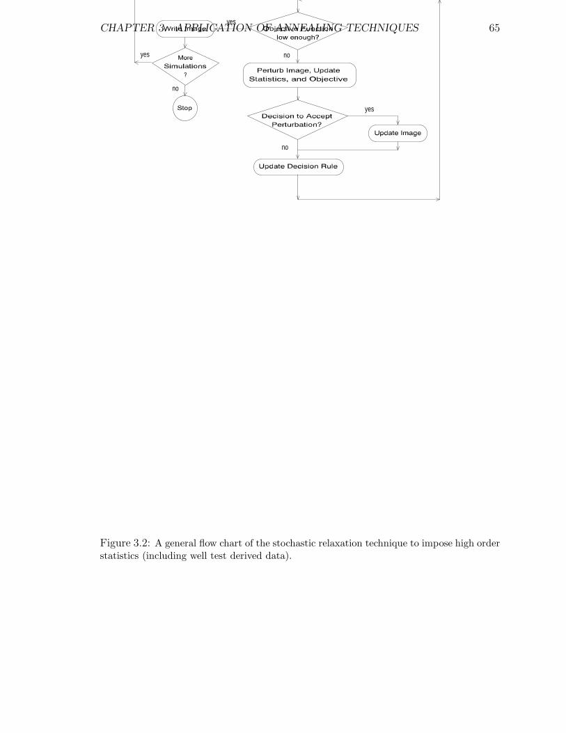
CHAPTER 3. APPLICATION OF ANNEALING TECHNIQUES 65
yes
no
no
yes
no
yes
Figure 3.2: A general flow chart of the stochastic relaxation technique to impose high orderstatistics (including well test derived data).

CHAPTER 3. APPLICATION OF ANNEALING TECHNIQUES 66
ways:
1. A different realization can be generated for each new simulation with
each nodal value drawn at random from the stationary cdf F (z). This
is straightforward and very fast.
2. The same input image, read directly from an input file, could be used as
the starting point for all realizations. Depending on the application this
may artificially narrow the output space of uncertainty.
3. Different initial images, read from an input file, could be used (e.g., various
sequential indicator simulation realizations could be taken and modified
with annealing to integrate additional prior information). These images
could be obtained from any source including output from a previous sasim
run.
Compute Initial Image Statistics: As discussed in the next section it is impor-
tant to update rather than recompute image statistics; however, an initial global
calculation is required before updating can take place. Note that the initial im-
age statistics may be both “control” values and “realization” values.
Compute Initial Objective Function: At this point all “control” and “realiza-
tion” values for each component of the global objective function are known.
Each component of the global objective function is calculated and weighted so
that all components may be lowered to zero during the optimization/simulation.
Details of the components entering the objective function and their weighting
scheme are given in section 3.2.
Objective Function Low Enough?: When the objective function has been low-
ered enough, or if attempts to improve the image are sufficiently discouraging,
the realization will be written to the output file. At that point the program will
begin the next simulation if more simulations are called for, or it will stop.
Perturb Image, Update Statistics and Objective: One of the following three
perturbation mechanisms is performed a specified number of times:

CHAPTER 3. APPLICATION OF ANNEALING TECHNIQUES 67
1. The values at two nodal locations ui and uj can be swapped.
2. The value at a node location ui is replaced by a random drawing from the
global stationary cdf F (z).
3. The value at a node location ui is replaced by a random drawing from a
local conditional ccdf F (ui; z) (this approach is documented by Srivastava
in [125]). The ccdf F (ui; z) is arrived at by a local weighted average or
indicator kriging. The local kriging weights are required input to sasim.
The decision rule is applied after a given number of perturbations (set by the
user). After each perturbation all components in the objective function, that
can be updated locally, are updated. All components that require a global
recalculation are updated just before the decision rule is applied.
Decision to Accept Perturbation: The acceptance criteria of simulated anneal-
ing, threshold accepting, or MAP simulation may be applied. That is, all per-
turbations (or series of perturbations) that decrease the objective function are
accepted and those that increase the objective function are accepted with the
following probability:
• Simulated Annealing (SA): P{accept} = eOold−Onew
t with the temperature
parameter t controlled by either a default annealing schedule or one preset
by the user.
• Maximum A Posteriori (MAP): P{accept} = 0 whenever the objective
function has increased.
• Threshold Accepting (TA): P{accept} = 1 if Oold − Onew < threshold ; 0,
otherwise. As the simulation proceeds the threshold is decreased with a
user defined schedule.
Update Image: The image, the image statistics, and the image objective function
are updated if the perturbation is accepted.
Update Decision Rule: In the case of simulated annealing and threshold accept-
ing the decision rule is updated after every perturbation (whether accepted or

CHAPTER 3. APPLICATION OF ANNEALING TECHNIQUES 68
not). In many cases the decision rule remains unchanged. In certain cases, this
updating will set the current objective function to zero to force the algorithm
to stop perturbing the image and move to the next simulation.
Local conditioning data are honored by fixing them in all prior realizations and
leaving then unperturbed:
z(l)(uα) = z(uα), ∀l, α = 1, . . . , n
Although conditioning to local data is very straightforward, experience has shown
that honoring local conditioning statistics may require special consideration in the
objective function. The issue of conditioning is discussed in more detail in Chapter
4.
3.2 The Objective Function
Annealing techniques rely on many, often millions, of perturbations to achieve a final
acceptable realization. The implications are that each component of the objective
function must be reasonably simple and there should not be too many components nor
conflicting components. In general, it will be essential to replace a global recalculation
of each component with a local updating; otherwise, the required computer time may
become excessive.
It is often possible to replace global recalculations with local updating since most
spatial statistics interact with only a limited number of other elements in the system.
For example, consider the variogram for a specific lag h:
γ(h) =1
2N(h)
N(h)∑i=1
[z(u) − z(u + h)]2 (3.1)
The number of pairs N(h) contributing to the variogram depends on the size of the
grid and the separation vector h. For example, vector h as a unit distance xsiz in
the x-direction of a square nx = 200 by ny = 200 grid. A global calculation of
γ(h) would require an evaluation of N(h) = (nx − 1) · ny = 39800 pairs of values.
However, when any one value is perturbed only two pairs in γ(h) must be updated.
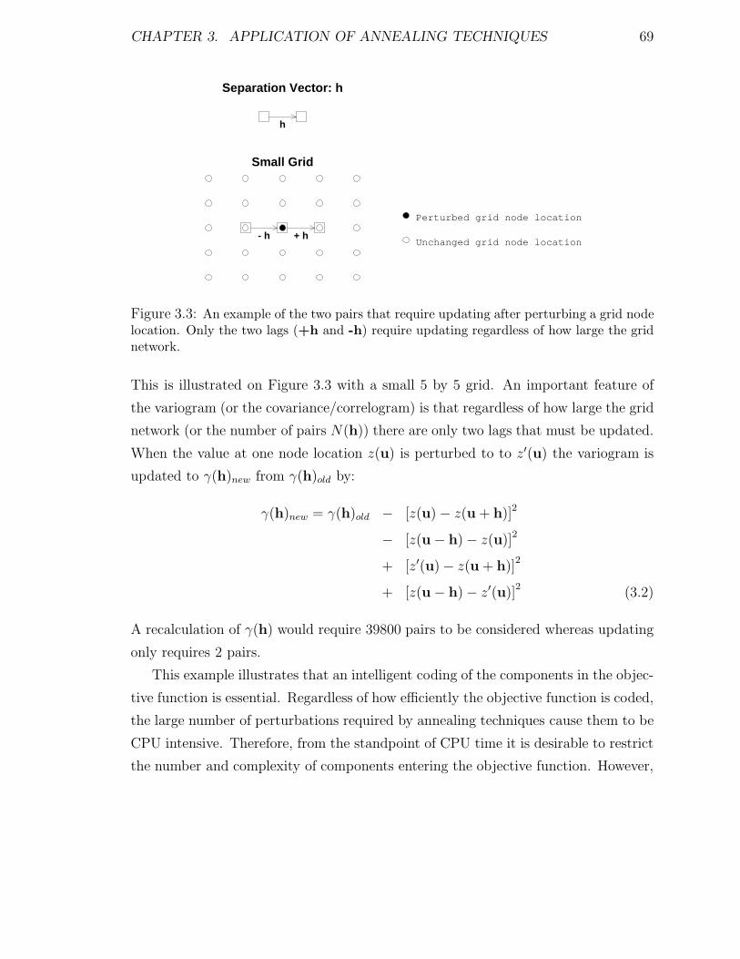
CHAPTER 3. APPLICATION OF ANNEALING TECHNIQUES 69
Separation Vector: h
h
Small Grid
Unchanged grid node location
Perturbed grid node location
+ h- h
Figure 3.3: An example of the two pairs that require updating after perturbing a grid nodelocation. Only the two lags (+h and -h) require updating regardless of how large the gridnetwork.
This is illustrated on Figure 3.3 with a small 5 by 5 grid. An important feature of
the variogram (or the covariance/correlogram) is that regardless of how large the grid
network (or the number of pairs N(h)) there are only two lags that must be updated.
When the value at one node location z(u) is perturbed to to z′(u) the variogram is
updated to γ(h)new from γ(h)old by:
γ(h)new = γ(h)old − [z(u) − z(u + h)]2
− [z(u − h) − z(u)]2
+ [z′(u) − z(u + h)]2
+ [z(u − h) − z′(u)]2
(3.2)
A recalculation of γ(h) would require 39800 pairs to be considered whereas updating
only requires 2 pairs.
This example illustrates that an intelligent coding of the components in the objec-
tive function is essential. Regardless of how efficiently the objective function is coded,
the large number of perturbations required by annealing techniques cause them to be
CPU intensive. Therefore, from the standpoint of CPU time it is desirable to restrict
the number and complexity of components entering the objective function. However,

CHAPTER 3. APPLICATION OF ANNEALING TECHNIQUES 70
this may be contrary to the goal of integrating a maximum amount of prior informa-
tion. Given a slow technique and a fast technique that are equally good (see section
2.2), the fast technique is clearly preferred1. A very slow technique may be preferred
if it accounts for more prior information or it allows a more complete sampling of the
space of uncertainty. One hour of workstation CPU time to generate a realization,
versus one second, would be acceptable only if the realization generated in an hour is
significantly better. Given the exponential increase in computer speed over the past
few years and projected future increases there is no reason to limit artificially the
development of annealing programs to too simple objective functions.
In general, the overall objective function O is made up of the weighted sum of C
components:
O =C∑
c=1
wcOc (3.3)
where wc and Oc are the weights and component objective functions respectively. The
component objective functions measure how certain features of the simulated image
differ from the desired control or reference properties. For example, one component
could be a measure of difference between a variogram function modeled from actual
data and the experimental variogram function of the realization, a second component
could measure reproduction of a particular multiple-point statistic intended to reflect
the short scale structure (see section 3.3), and a third component could measure the
fidelity to a well test-derived effective property (see section 3.4).
Each component objective function Oc could be expressed in widely different
units of measurement. For example, a component measuring variogram departure
(Oc1 =∑[
γreference − γrealization
]2) may be in units of variance squared, while a
component measuring the fidelity to a well test-derived effective permeability (Oc2 =
[Kreference − Krealization]2) may be in units of millidarcies squared. Equally weighting
components with widely different units will cause the component with the largest
units to dominate the global objective function.
The purpose behind the weights wc, c = 1, . . . , C, is to have each component c play
1The speed of a technique is the time required to set it up plus the actual CPU time needed togenerate the realizations.

CHAPTER 3. APPLICATION OF ANNEALING TECHNIQUES 71
an equally important role in the global objective function2. Note that the magnitude
of the objective function only indirectly affects the decision to accept or reject a
perturbation: all decision rules are based on the change to the objective function,
i.e.,
∆O = Onew − Oold
∆O =C∑
c=1
wc∆Oc =C∑
c=1
wc [Ocnew − Ocold]
The weights wc, c = 1, . . . , C are established so that, in average, each component con-
tributes equally to the change in the objective function ∆O. That is, each weight wc
is inversely proportional to the average change of that component objective function:
wc =1¯|∆Oc|
, c = 1, . . . , C (3.4)
In practice, the average change of each component |∆Oc| can not be computed
analytically; however, it can be numerically approximated by evaluating the average
change of M (say 1000) independent perturbations:
|∆Oc| =1
M
M∑m=1
|O(m)c − Oc|, c = 1, . . . , C (3.5)
where |∆Oc| is the average change for component c, O(m)c is the perturbed objective
value, and Oc is the initial objective value. Each of the M perturbations m = 1, . . . , M
arises from the perturbation mechanism that will be employed for the annealing
simulation.
The overall objective function used in sasim is finally written as,
O =1
O(0)·
C∑c=1
wc · Oc (3.6)
where the weights wc given in equation (3.4) are computed at the beginning of the
simulation (annealing) procedure. The objective function O is restandardized by
its initial value, O(0), so that it always starts at 1.0 and a standardized annealing
schedule3 may be used.
A number of considerations regarding the objective function should be noted:
2The program sasim also allows the user to change arbitrarily the relative importance of eachcomponent.
3The initial temperature t0 is also set to 1.0 for simulated annealing.

CHAPTER 3. APPLICATION OF ANNEALING TECHNIQUES 72
• The gradient or rate of decrease of each component is not accounted for in the
weights (3.4). One component may quickly go to zero while another could take
much longer. Consequently, the weights may need to be re-evaluated periodi-
cally during the simulation.
• In addition to weighting each component on the basis of its average change
(|∆Oc|) one could also consider the relative importance of each component. For
example, it may be more desirable to have a good variogram match than repro-
ducing partial quadrivariate information obtained from a questionable training
image. Unequal weighting is particularly useful in cases where the objective
function cannot be lowered close to zero, e.g., due to conflicting components.
sasim allows the user to define arbitrarily the relative weights of each compo-
nent.
• Another question is whether the components should receive the same weight for
the entire duration of the optimization procedure. For example, at the begin-
ning it may be advantageous to establish the coarse features by preferentially
weighting two-point statistics, then, at the end multiple-point statistics and well
test results could be given more weight to establish the small scale details. This
has not been considered in sasim and could be a subject of future research.
Annealing techniques make no explicit reference to a random function (RF) model;
however, the very act of generating multiple spatial realizations defines an implicit
multivariate distribution or RF model. This implicit RF model depends on the com-
ponents entering the objective function, and on other implementation decisions such
as the initial image, the perturbation mechanism, and the decision rule. An effort
will be made in the case studies of later chapters to understand better the implicit
RF model underlying annealing techniques.
The following two sections describe how multiple-point statistics and well test-
derived effective permeability may be expressed as component objective functions.

CHAPTER 3. APPLICATION OF ANNEALING TECHNIQUES 73
One-Point Configuration
Two-Point Configuration
Three-Point Configuration
Four-Point Configuration
Nine-Point Configuration
Figure 3.4: Examples of 1, 2, 3, 4, and 9-point configurations. Each gray square representsa grid node location. The black dot in the center of a grid node location represents the nullvector.
3.3 Multiple-Point Statistics
There are few published references [85] and little practical experience with multiple-
point spatial statistics beyond the bivariate or two-point level; intuition about which
multiple-point statistics are appropriate to characterize any particular geological fea-
ture will develop with time. In section 2.4, multiple-point statistics were considered
necessary to model many commonly encountered geological features where the pre-
dominant characteristics are curvilinear and connected beyond the two-point level.
Developing a program, such as sasim, with the capability to integrate multiple-point
statistics will allow the evaluation of the importance of that information. Recall that
the importance of an input information is measured in terms of the output space of
uncertainty and not necessarily in the appearance of the stochastic models.
Throughout this dissertation a multiple-point or N -point configuration is defined
by N separation lag vectors h1, . . . ,hN , with by convention h1 = 0. Figure 3.4 shows
examples of 1, 2, 3, 4, and 9 point configurations.
The first multiple-point statistic coded into sasim is the semivariogram (2.19),
which carries the same two-point information as the the covariance or correlogram.

CHAPTER 3. APPLICATION OF ANNEALING TECHNIQUES 74
The semivariogram for lag hl is defined as:
γ(hl) =1
2 · N(hl)
N(hl)∑[Z(u) − Z(u + hl)]
2 (3.7)
Where any number l = 1, . . . , L of separation vectors hl may be specified, N(hl) is the
number of pairs for lag hl, and γ(hl) is the semivariogram for lag hl. A component c
in the objective function O is then:
Oc =L∑
l=1
|γcontrol(hl) − γrealization(hl)| (3.8)
with γcontrol(hl) being the control or reference semivariogram and γrealization(hl) the
experimental semivariogram of the candidate realization.
The second multiple-point statistics coded into sasim are multiple-point non-
centered indicator covariances. The indicator transform of a categorical variable is
defined as, see also (2.11):
I(u; k) =
1, if Z(u) ∈ category k
0, otherwise(3.9)
The indicator transform of a continuous variable may be constructed in one of two
ways:
I(u; z) =
1, if Z(u) ≤ z
0, otherwise(3.10)
J(u; z) =
1, if Z(u) > z
0, otherwise(3.11)
with I(u; z) = 1 − J(u; z).
The multiple-point non-centered indicator covariance defined by N lag separation
vectors h1, . . . ,hN , with by convention h1 = 0, is defined as:
ϕI(h1, . . . ,hN ; z1, . . . , zN) = E
N∏j=1
I(u + hj ; zj)
(3.12)
The non-centered indicator covariance for J is similarly defined:
ϕJ(h1, . . . ,hN ; z1, . . . , zN) = E
N∏j=1
J(u + hj ; zj)
(3.13)

CHAPTER 3. APPLICATION OF ANNEALING TECHNIQUES 75
In general, ϕI and ϕJ contain different information: ϕI is the probability of the N
values being jointly below the given threshold values whereas ϕJ is the probability of
the N values being jointly above the given threshold values. Recall from section 2.3
equation (2.15), that the connectivity function of Journel and Alabert [85] corresponds
to an I indicator defined at the same cutoff zc with the N -points spatially separated
by multiples of the same lag separation vector h.
Given L such multiple-point covariances a component c of the objective function
O is then:
Oc =L∑
l=1
| ϕcontrolI (h
(l)1 , . . . ,h
(l)N ; z
(l)1 , . . . , z
(l)N )
− ϕrealizationI (h
(l)1 , . . . ,h
(l)N ; z
(l)1 , . . . , z
(l)N ) | (3.14)
Where each of the l = 1, . . . , L contributions is a specific N (l)-point indicator covari-
ance. Note that ϕJ could be used in place of ϕI .
The univariate cdf F (z), at a specific threshold z, may be expressed as a non-
centered indicator covariance ϕI(h1; z) with N = 1 and h1 the null vector. Thus, the
univariate cdf may explicitly enter the objective function in the form of non-centered
indicator covariances.
Traditional bivariate indicator covariances, CI(h; z1, z2), may also enter the ob-
jective function as specific N = 2 non-centered multiple-point indicator covariances:
ϕI(h1,h; z1, z2) = CI(h; z1, z2) + F (z1) · F (z2)
where ϕI(h1,h; z1, z2) is the non-centered indicator covariance, h1 is the null vector,
h is the pair separation vector, and z1 and z2 are indicator thresholds.
Note that an N -point statistic includes lower order statistics M < N whose config-
urations are part of the N -point geometric configuration. For example, when consider-
ing non-centered two-point indicator covariances it is unneccessary to allow explicitly
for the univariate cdf at the same thresholds.
Specific non-centered indicator covariances ϕI(h1, . . . ,hN ; k1, . . . , kN) for categor-
ical variables may also enter the objective function. When considering a categorical
variable that takes outcomes k = 1, . . . , K, the collection of all direct and cross non-
centered indicator covariances is referred to as a multiple-point histogram denoted

CHAPTER 3. APPLICATION OF ANNEALING TECHNIQUES 76
with notation f (see also (2.17) in section 2.3.1):
ϕI(h1, . . . ,hN ; k1, . . . , kN) = f(h1, . . . ,hN ; k1, . . . , kN) (3.15)
∀ k1, . . . , kN = 1, . . . , K
These cross non-centered indicator covariances can be interpreted as the set of all
transition probabilities for the K categories for a pattern described by the N vectors
h1, . . . ,hN .
Any number L of multiple-point histograms, specified as configurations of N (l)
points defined by N (l) separation vectors h1, . . . ,hN(l), may be considered in the
objective function as:
Oc =L∑
l=1
K∑k1=1
K∑k2=1
· · ·K∑
kN(l)=1
| f control(h(l)1 , . . . ,h
(l)N ; k1, . . . , kN(l))
− f realization(h(l)1 , . . . ,hN(l); k1, . . . , kN(l)) | (3.16)
There is no essential difference between N -point covariances, which enter the ob-
jective as (3.14), and N -point histograms which enter as (3.16). The difference in
the sasim program is that the thresholds for each multiple-point covariance must
be explicitly specified whereas selecting a multiple-point histogram causes sasim to
consider automatically all possible classes or combinations of threshold values.
Given an N -point histogram of a categorical variable that can take one of K
outcomes, there are KN classes. Table 3.1 shows the number of classes for different
K and N values. Although there is a practical limit to the number N of points
that can be considered, sasim has been coded with no such restriction (only the
dimensioning will have to be changed when RAM memory in the gigabyte range
becomes available).
Commonly, the KN classes are assigned a one dimensional index for computer
storage and to allow N -point histograms to be displayed in the traditional way, i.e., as
bar charts of frequency versus class number. Given N categorical variables z(hi), i =
1, . . . , N that can take values k = 1, . . . , K a unique one dimensional index may be
computed as:
index = 1 +i=N∑i=1
[z(hi) − 1] · Ki−1 (3.17)

CHAPTER 3. APPLICATION OF ANNEALING TECHNIQUES 77
N=2 N=3 N=4 N=9K=2 4 8 16 512K=3 9 27 81 19,683K=4 16 64 256 262,144K=5 25 125 625 1,953,125K=6 36 216 1,296 10,077,696K=7 49 343 2,401 40,353,607K=8 64 512 4,096 134,217,728K=9 81 729 6,561 387,420,489
K=10 100 1,000 10,000 1,000,000,000
Table 3.1: The number KN of classes for various multiple-point statistics (N = 2, 3, 4, 9)and numbers of categories (K = 2, 3, 4, 5, 6, 7, 8, 9, 10).
Each index value corresponds to a unique pattern, i.e., a particular combination of
the N points. For example, given N = 4 and K = 2 there are KN = 24 = 16 possible
patterns with indices given by:
index = z(h1) + [z(h2) − 1] · 2 + [z(h3) − 1] · 4 + [z(h4) − 1] · 8 (3.18)
If the four points constitute a square configuration, with k = 1 corresponding to
white, and k = 2 to black, the 16 patterns are enumerated in Table 3.2 and shown
graphically on Figure 3.5.
This indexing convention will be used throughout the code and text of this dis-
sertation.
Updating Multiple-Point Statistics
As discussed in section 3.2, an important practical criterion for any statistic is that
is should allow the objective function to be updated locally rather than having to be
globally recalculated after each local perturbation. Equation (3.2) in section 3.2 shows
how the semivariogram could be locally updated. It turns out that local updating is
also possible for multiple-point statistics.
Let Z be a categorical variable that can take one of K integer categories k =

CHAPTER 3. APPLICATION OF ANNEALING TECHNIQUES 78
index z(h1) z(h2) z(h3) z(h4)1: 1 1 1 12: 2 1 1 13: 1 2 1 14: 2 2 1 15: 1 1 2 16: 2 1 2 17: 1 2 2 18: 2 2 2 19: 1 1 1 2
10: 2 1 1 211: 1 2 1 212: 2 2 1 213: 1 1 2 214: 2 1 2 215: 1 2 2 216: 2 2 2 2
Table 3.2: The one dimensional indices of a four-point histogram with K=2.

CHAPTER 3. APPLICATION OF ANNEALING TECHNIQUES 79
1 2
3 4Locations: h_1, h_2, h_3, h_4
index = 1 index = 2 index = 3 index = 4
index = 5 index = 6 index = 7 index = 8
index = 9 index = 10 index = 11 index = 12
index = 13 index = 14 index = 15 index = 16
Figure 3.5: An illustration of the indexing convention for a four-point configuration: N =4,K = 2. The configuration is illustrated at the top of the figure followed by all 16 possiblepatterns (white and black correspond to k = 1 and 2 respectively).

CHAPTER 3. APPLICATION OF ANNEALING TECHNIQUES 80
1, . . . , K. Consider any realization with values z(ui), i = 1, . . . , N and any arbi-
trary N -point histogram defined by N lag separation vectors h1, . . . ,hN with, by
convention, h1=0. This specific multiple-point histogram is globally calculated from
the starting image before any perturbation, i.e., all of the following proportions are
enumerated:
f(h1, . . . ,hN ; k1, . . . , kn) =
proportion of patterns z(h1) = k1, . . . , z(hN ) = kN (3.19)
∀k1, . . . , kN = 1, . . . , K
Now, consider that a particular nodal value z(u) = k is perturbed into z(u) = k′.
The multiple-point histogram has changed in that all configurations involving location
u are now different. The updating concept consists of subtracting what was there
before and adding what comes in after the perturbation.
For a two point statistic, defined by two vectors h1 = 0 and h2, there are two
configurations where the pattern has changed (as shown on Figure 3.3). The first is
generated by offsetting the configuration by minus the first lag vector h1:
point one : (u + h1) − h1
point two : (u + h2) − h1
The second configuration that has changed is that generated by offsetting the config-
uration by minus the second lag vector h2:
point one : (u + h1) − h2
point two : (u + h2) − h2
For both of these configurations the original pattern with z(u) = k is subtracted from
the global statistic and the new pattern with z(u) = k′ is added in.
As another example, consider the specific three-point statistic shown on Figure 3.6.
Perturbing the central grid node location, shown by the black dot, changes three
patterns/configurations. The first configuration is that generated by offsetting the

CHAPTER 3. APPLICATION OF ANNEALING TECHNIQUES 81
configuration of N = 3 points by lag −h1 (a null vector by convention):
point one : (u + h1) − h1
point two : (u + h2) − h1
point three : (u + h3) − h1
The second configuration is that generated by offsetting the N = 3 point configuration
by lag −h2:
point one : (u + h1) − h2
point two : (u + h2) − h2
point three : (u + h3) − h2
The third and final configuration that needs updating, regardless of the size of the
grid network, is that generated by offsetting the N = 3 point configuration by lag
−h3:
point one : (u + h1) − h3
point two : (u + h2) − h3
point three : (u + h3) − h3
In general, for any N -point statistic there are N configurations where the pattern
changes if a nodal value z(u) = k is perturbed to z(u) = k′. Updating the N -
point statistic amounts to subtracting the previous contribution and adding the new
contribution for all N configurations:
pattern of Npoints offset by − h1
pattern of Npoints offset by − h2
...
pattern of Npoints offset by − hN
Within the sasim program the subtraction and addition are done simultaneously
for each of the N configurations. The updating principle is the same regardless of the
specific multiple-point statistic and how many points N are involved.

CHAPTER 3. APPLICATION OF ANNEALING TECHNIQUES 82
A Specific Three-Point Statistic
1 2
3
First Pattern to Update
Unchanged grid node location
Perturbed grid node location
Second Pattern to Update
Unchanged grid node location
Perturbed grid node location
Third Pattern to Update
Unchanged grid node location
Perturbed grid node location
Figure 3.6: An example of the three-point configurations that need updating after a per-turbation.

CHAPTER 3. APPLICATION OF ANNEALING TECHNIQUES 83
1
2 3
4
Figure 3.7: The four point configuration, and three direction vectors, corresponding to theexamples shown on Figures 3.8, 3.9, and 3.10.
Examples with Four-Point Histograms
For an additional acquaintance with multiple-point statistics consider the four-point
histogram corresponding to four points in a unit square configuration as in Figure 3.7.
Three examples of four point histograms with K = 2 (white and gray) are shown on
Figure 3.8. All three images are 200 by 200 pixels and have exactly 50% white and
50% gray pixels. The four point histogram is shown to the right of each image. There
are Kn = 24 = 16 classes indexed from 1 through 16. Note that the horizontal axes
on each histogram plot is the one dimensional index (3.17) of each class. The upper
image shows 20 alternating white and gray stripes each 5 pixels thick. There are only
four non-zero classes in the corresponding four-point histogram (all white, all gray,
2 white over 2 gray, and 2 gray over 2 white). The central image shows 5 by 5 gray
squares located at random. All classes in the four-point histogram are represented;
the histogram shows only six significant classes, all white, all gray, 2 white over 2 gray,
2 gray over 2 white, 2 gray beside 2 white, and 2 white beside 2 gray). The random
image, shown at the bottom, leads to an equal probability to be in each class4.
Figure 3.9 attempts to quantify visually how much information is carried in such
four-point histograms. The training image is shown at the top of the figure. The
two middle realizations are conditional to the two-point histogram in one lag in all
directions (horizontal, vertical, and the two diagonal directions). The two lower real-
izations are conditional to one particular four-point statistic (a 2 by 2 pixel configu-
ration as in Figure 3.7). The two-point statistics cover the same areal extent as the
four-point information but clearly do not carry the same information. The difference
4This would not be true if there was an unequal fraction of white and gray pixels

CHAPTER 3. APPLICATION OF ANNEALING TECHNIQUES 84
Stripes
Fre
quen
cy
class
0 4 8 12 16
.000
.100
.200
.300
.400
Stripes: Four Point Histogram
Squares
Fre
quen
cy
class
0 4 8 12 16
.000
.100
.200
.300
.400
Squares: Four Point Histogram
Random
Fre
quen
cy
class
0 4 8 12 16
.0000
.0100
.0200
.0300
.0400
.0500
.0600
Random: Four Point Histogram
Figure 3.8: Three illustrations of four-point histograms. The four-point histogram is forfour-points in a unit square configuration. The images are shown on the left and the fourpoint histograms on the right.

CHAPTER 3. APPLICATION OF ANNEALING TECHNIQUES 85
quantified in terms of output uncertainty is given in Chapter 5.
A second example shown on Figure 3.10 compares images generated with two-
point and four-point statistics. Two-point statistics for a unit lag in each direction
were retained to condition the two middle realizations and the four-point information
corresponding to a unit square configuration was retained for the two lower real-
izations. The areal coverage of both sources of information is the same, yet, the
four-point statistic seems to capture more of the salient features of the upper training
image such as the diagonal banding.
In practice, the multiple point configurations to be used must be chosen as char-
acteristics of the geometric features deemed important. For example, the four point
configuration shown on Figure 3.7 or any arbitrary configuration such as the six-point
or hexivariate configurations shown on Figure 3.11 may be retained. The specification
of multiple-point statistics requires the number of points N and the N −1 separation
lag vectors (offsets from the first vector h1 set to zero).
A combination of different “multiple” information is recommended. For example,
consider retaining two-point statistics specified for larger separation distances with
some multiple-point statistics used for short scale features. This point is further
developed with some example applications in Chapter 5.
3.4 Well Test-Derived Effective Permeability
Well test data is already quantified in the sense that the pressure response to some
flow impulse is measured with extremely precise gauges [66, 111]. The challenge is to
interpret this detailed pressure response and relate it to the petrophysical properties
that are important for flow modeling. Interpretation of the pressure transient is
necessary. Early-time effects such as wellbore storage and near wellbore effects such
as the skin effect are not relevant to the reservoir modeling problem being addressed
in this dissertation. Similarly, the modeling of reservoir boundaries and other late-
time effects could be accounted for deterministically and are not considered in this
research. For example, fault boundaries can be explicitly entered into the numerical
model of the reservoir. Moreover, the effects of other wells can also be explicitly

CHAPTER 3. APPLICATION OF ANNEALING TECHNIQUES 86
Berea Sandstone Training Image
Two-point Statistics Two-point Statistics
Four-point Statistics Four-point Statistics
Figure 3.9: The Berea control pattern, two realizations using two-point information, andtwo realizations using four-point information. Both the two-point and four-point informa-tion cover the same extent (a unit pixel in each direction).

CHAPTER 3. APPLICATION OF ANNEALING TECHNIQUES 87
Training Image
Two-point Statistics Two-point Statistics
Four-point Statistics Four-point Statistics
Figure 3.10: A difficult control pattern, two examples using partial bivariate information,and two examples using quadrivariate information. The bivariate data was retained for 25lags in four directions. The quadrivariate data was a 2 by 2 pixel configuration.

CHAPTER 3. APPLICATION OF ANNEALING TECHNIQUES 88
Six Points: discontinuous pattern
1 2
3 4 5 6
Six Points: curvilinear pattern
1
2 3
4 5 6
Six Points: rectangular pattern
1 2 3
4 5 6
Six Points: linear pattern
1 2 3 4 5 6
Figure 3.11: Examples of 6-point configurations. In practice, the configuration is cus-tomized to reflect the spatial features deemed important.
accounted for by digitizing the drainage area of each well.
One way of conditioning stochastic reservoir models to a well test response would
be to discard all models that do not yield a forward simulated well test response close
enough to the actual measured pressure response. Such selection procedures may be
practical when building models with a single well test; however, it is not practical in
the presence of multiple well test interpretations, some with more advanced multirate
tests which inform a number of different permeability averages near the well. In
general, a prohibitively large number of realizations would be required to find a few
that simultaneously match all well test data.
The idea of this research is to take realizations that already match other available
data (e.g., core, well logs, seismic) and modify them, with annealing, to match addi-
tionally the well test responses. Given the computer resources available at this time
it is not possible to perform a full 3-D flow simulation after every perturbation called
for in the annealing algorithm; such 3-D flow simulation would amount to a global
updating. Somehow the well test data must be translated into an easily updateable
property while retaining the flexibility to differentiate a wide variety of heterogeneous
systems encountered in practice.

CHAPTER 3. APPLICATION OF ANNEALING TECHNIQUES 89
The absolute effective permeability near the well bore inferred from the well test
response is a critical parameter provided by well test interpretation. The essential
assumptions and mathematical basis for well test interpretation must be discussed
before presenting a quantification of the permeability averaging process associated to
a well test.
Pressure transient well tests are performed by generating some flow rate impulse
in the reservoir (e.g., start production, change the flow rate, stop production, . . . )
and measuring the pressure response. Well test interpretation or pressure transient
analysis consists of interpreting the pressure response by using some appropriate
mathematical model to relate the pressure response (output) to flow rate history (in-
put) [66]. Provided that the mathematical model is appropriate the model parameters
can be associated to certain reservoir parameters.
Pressure transient analysis is based on what seem a-priori like limiting assumptions
[66, 103], these being,
• There is radial flow into a well opened over the entire vertical thickness of the
formation.
• The formation is homogeneous and isotropic with constant porosity and con-
stant permeability (both are independent of pressure).
• The fluid has a small and constant compressibility and a constant viscosity.
• The pressure gradients are small and the gravity forces are negligible.
Some of these assumptions may be relaxed by considering variable transformations,
adding terms to the flow equations to account for non-Darcy effects, or by considering
more sophisticated flow equations.
The equation governing fluid flow given the preceding assumptions is the following:
∂2p
∂r2+
1
r
∂p
∂r=
φµc
k
∂p
∂t(3.20)
where p is pressure, r is the radial distance from the wellbore, φ is the porosity, µ
is the viscosity, c is the fluid compressibility, k is the absolute permeability, and t is
time.

CHAPTER 3. APPLICATION OF ANNEALING TECHNIQUES 90
In the case of an infinite reservoir and a line source well the pressure solution to
this equation may be written.
p(r, t) = pi − qµ
2πkh
{−1
2Ei
(−φµcr2
4kt
)}(3.21)
where Ei is the exponential integral function,
−Ei(−x) =∫ ∞
x
e−u
udu
The exponential integral function is approximated very well by a log function for
all but early times, therefore, we may write (see equation 2.32, page 11, Matthews
and Russell [103]):
p(r, t) = pi − qµ
4πkh
[ln
kt
φµcr2+ 0.80907
](3.22)
In the previous development the standard SPE notations have been used as much as
possible [123]. Recall that p(r, t) is the pressure (psi) at radial distance r (feet) and
time t (hours), pi is the initial reservoir pressure (psi) (the subscript i is not to be
confused with a grid node index), q is the flow rate (STB/d), µ is the fluid viscosity
(cp), k is the absolute permeability (md), h is the formation thickness (feet), φ is
the porosity (pore volume/bulk volume), and c is the compressibility (/psi). In many
situations dimensionless variables are used to simplify the notation and to provide
solutions that are independent of any particular unit system [66].
The dimensionless pressure pD is defined in oilfied units as:
pD =kh
141.2qBµ(pi − pwf) (3.23)
where all variables are as above and pwf is the well flowing pressure (the pressure
directly measured in a well test). In a consistent unit set, pD is defined as:
pD =2πkh
qBµ(pi − pwf) (3.24)
The dimensionless time tD is defined in oilfield units as:
tD =0.000264kt
φµctr2w
(3.25)

CHAPTER 3. APPLICATION OF ANNEALING TECHNIQUES 91
where all variables are as above and rw is the wellbore radius in feet. In a consistent
unit set, tD is defined as:
tD =kt
φµctr2w
(3.26)
Finally, the dimensionless radius rD is defined as:
rD =r
rw(3.27)
Given a well test performed in the field, and estimates for µ, h, φ, and c, it is
possible to estimate an effective permeability ke that relates to some volume near
the well. The idea proposed by Alabert [7] and developed in this dissertation is to
impose this effective permeability on stochastic models through the objective function
of annealing-based techniques. An important issue that must be addressed is the
volume and type of averaging represented by the well test-derived permeability.
3.4.1 Empirical Relationship for the Well Test Effective Per-
meability
The nature of the radial averaging process depends on the exact spatial configuration
of the reservoir attributes; therefore, in all rigor, a full 3-D flow simulation is required
to quantify this averaging process. In practice, the constraint of annealing calls for a
very fast yet reasonably accurate evaluation of each parameter entering the objective
function. It would not be practical to perform a full 3-D flow simulation to obtain the
effective permeability after each (set of) perturbation(s). An empirical scaling law
must be devised that relates the well test-derived effective permeability to elementary
block absolute permeability values.
Alabert [7] proposes a power average of the block permeabilities within a specified
averaging volume V to model the full non-linear averaging of block permeabilities as
measured by a well test. The assumption is that the elementary block permeability
values average linearly after a non-linear power transformation, i.e.,
k(ω) =
1
N
∑ui∈V
k(ui)ω
1ω
(3.28)

CHAPTER 3. APPLICATION OF ANNEALING TECHNIQUES 92
Where k(ω) is the ω-power average permeability of the N permeability values k(ui), i =
1, . . . , N , at locations ui within the volume of interest V . The power ω varies between
the bounding values of -1 and 1 corresponding to the harmonic and arithmetic aver-
ages respectively. Note that the geometric average is obtained for ω → 0.0. Previous
work with power averaging [27, 36, 35, 88, 94, 95] has shown that the averaging power
parameter ω is remarkably robust.
Once the averaging volume V and the averaging type, as characterized by the
averaging power ω, are known a component objective function is considered as:
Oc = [kwelltest − krealization]2 (3.29)
where kwelltest is the well test-derived effective permeability and krealization is the ef-
fective permeability of the candidate realization, see equation (3.28). When the value
at one node location k(u) is perturbed to k′(u) the effective permeability is updated
to knewrealization from kold
realization by:
knewrealization =
[(kold
realization
)ω − 1
Nk(u)ω +
1
Nk′(u)ω
] 1ω
(3.30)
This fast numerical updating replaces a full flow simulation to arrive at a new
effective permeability for each candidate realization. To implement this numerical
approximation both the averaging volume V and averaging power ω must be defined.
The Averaging Volume
To define the appropriate averaging volume it is necessary to consider the portion of
the pressure response used to derive the well test effective permeability kwelltest. In
practice, kwelltest is obtained by interpreting the pressure response during the time at
which the response resembles infinite-acting radial flow. Early-time effects such as
wellbore storage and late-time boundary effects are not considered in the interpre-
tation. It is possible to define an inner radius rmin and an outer radius rmax that
correspond to the limits of infinite acting radial flow since the pressure response, at

CHAPTER 3. APPLICATION OF ANNEALING TECHNIQUES 93
any time t, may be related to block permeabilities within a time-dependent radius-
of-drainage r(t). Consider a typical pressure response shown on the Miller-Dyes-
Hutchinson (MDH) plot5 at the bottom of Figure 3.12. The pressure response be-
tween 1 hour and 10 hours is used to derive an estimate of the effective permeability
kwelltest. The inner and outer limits of the shaded region (on the schematic illustra-
tion of the reservoir) correspond to the radius-of-drainage at 1 hour and 10 hours
respectively.
Before proceeding with details of how to calculate rmin and rmax it is useful to
explain why the volume of investigation is an annular volume. Intuitively, it is rea-
sonable to expect that for a given well test duration the volume of investigation is
limited by an outer radius; however, the reason why the near wellbore permeability
values are excluded is less intuitive. First, it should be noted that the well test effec-
tive permeability is based on the pressure derivative during the infinite acting radial
flow portion of the response. The slope on the straight line fit through the response
on Figure 3.12 is linearly related to the permeability, i.e.,
ke = 162.6qBµ
|m|h (3.31)
where m is the slope of the semilog straight line. At any instant in time the pres-
sure derivative is informed by a particular annular volume centered at the wellbore.
Figure 3.13 shows the normalized weighting function, derived6 by Oliver [107], for
tD = 102, 104, and 106. By not considering the early time pressure response the block
permeability values near the wellbore do not contribute to the well test derived effec-
tive permeability. Figure 3.14 shows the contribution of the block permeability values
plotted as a function of the radial distance from the wellbore.
The time interval that the pressure response resembles infinite-acting radial flow is
easily determined by standard interpretation techniques 7. Evaluating the radius-of-
drainage r(t) at the time limits is not as straightforward; depending on the arbitrary
5A plot of pressure versus the logarithm of time.6The derivation calls for the permeability field to be expressed as a constant value plus a small
variation. The consequences of this assumption have not been evaluated since this weight functionis only used for explanation purposes.
7Note that the outer limit may be at the end of the test; boundary effects may not be seen on“short” well tests.

CHAPTER 3. APPLICATION OF ANNEALING TECHNIQUES 94
Miller-Dyes-Hutchinson Plot
Time, hrs
Pre
ssur
e, p
si
Early-time effects Late-time effectsInfinite Acting
Radial Flow
0.01 0.1 1 10 100
270.0
274.0
278.0
282.0
286.0
290.0
Plan View of the Reservoir
wellVo
lum
e Inform ed by Infinite Acting R
adial
Flo
w
Figure 3.12: A schematic illustration of the volume measured by a given well test inter-pretation. The inner and outer limits of the shaded region, on the schematic illustrationof the reservoir, correspond to the radius-of-drainage at 1 hour and 10 hours (the limits ofinfinite acting radial flow).

CHAPTER 3. APPLICATION OF ANNEALING TECHNIQUES 95
Normalized Weighting Function for Three tD values
Dimensionless Distance
Nor
mal
ized
Wei
ghtin
g F
unct
ion
td = 100 td = 10000 td = 1000000
1 10 100 1000 10000
0.00
0.10
0.20
0.30
0.40
Figure 3.13: The normalized weighting function versus the dimensionless radius rd forthree different instants in time.
Weight
Inner limits
Outer limits
Radial Distance Radial Distance
Figure 3.14: A schematic illustration of the radial weight function for the power averageapproximation to the well test effective permeability.
CHAPTER 3. APPLICATION OF ANNEALING TECHNIQUES 96
definition chosen for r(t), the radius can change by as much as a factor of 4. As
documented by Alabert [7] it will be necessary to calibrate the radius-of-drainage
r(t) by repeated flow simulations.
The radius-of-drainage defined below follows the classical formulation by van
Poollen [132] and Johnson [72]. The work of Alabert [7] and Oliver [107, 108] present
additional interpretations and numerical examples. The block permeabilities con-
tributing to the pressure response measured up to time t are approximately enclosed
by a circular volume centered at the well defined by a time-dependent radius r(t)
written as [7, 72, 132]:
r(t) = A
√ket
φµct
(3.32)
where A is a constant, ke is the reservoir permeability around the well, φ is the
porosity, µ is the fluid viscosity, and ct is the total compressibility. This relation
(3.32) implicity assumes that the heterogeneous permeability field is described by a
single permeability, i.e., ke is independent of time. Note that (3.32) can be written
in dimensionless units as:
rD(t) = A√
tD (3.33)
with rD and tD defined in equations (3.27) and (3.26).
Depending on the definition chosen for the radius-of-drainage the value of A varies
from 0.023 to 0.07 (for oil field units) or between 1.4 and 4.3 in consistent units.
Alabert [7], in the context of evaluating the averaging volume of a well test, and for
specified levels of discretization and test durations, found a robust optimal Aopt value
of 0.010 in oil field units (0.6 in consistent units). Thus, the annular volume V (A)
may be defined by rmin(A) and rmax(A) where A is taken as Aopt = 0.010 or calibrated
by repeated flow simulations.
The Averaging Power
The averaging power ω describes the type of averaging within the volume V (A). In
many cases, this averaging power is close to the geometric average (ω = 0). For
example, Butler [23] and Alabert [7] show cases where the effective permeabilities
obtained from classical well test analyses converge towards the geometric average. For

CHAPTER 3. APPLICATION OF ANNEALING TECHNIQUES 97
practical test durations and for complex heterogeneous permeability distributions, the
type of averaging can differ significantly from the geometric average.
The constant A = 0.010 and the averaging power ω = 0.0 may be used as first
approximations in equation (3.28) to calculate the effective permeability krealization.
However, in practice, both the constant A and the averaging power ω should be
calibrated ahead of time with the following calibration procedure:
1. Generate ns (20-100) multiple realizations of the permeability field with relevant
statistical properties.
2. Forward simulate a well test, with conditions as close as possible to those used in
the field to arrive at kwelltest, on each realization to obtain ns pressure response
curves.
3. Deduce an effective permeability ki, i = 1, . . . , ns from each pressure curve using
established well test interpretation techniques [66].
4. Compute average permeabilities k(A, ω)i, i = 1, . . . , ns for A values between
the practical bounding limits of 0.005 and 0.035 and for ω values between the
bounding limits of -1 and 1. For example, taking A-increments of 0.001 and
ω-increments of 0.05 would lead to
ns ·(
0.035 − 0.005
0.001+ 1
)·(
1.0 − (−1.0)
0.05+ 1
)= ns · 1271
calculations of k(ω, A) values.
5. Choose the pair (Aopt, ωopt) that yields the closest agreement between the refer-
ence ki, i = 1, . . . , ns values and the approximate k(Aopt, ωopt)i, i = 1, . . . , ns val-
ues. Alabert suggests taking the mean normalized absolute deviation (mNAD)
and the mean normalized error (mNE) as criteria for selecting (Aopt, ωopt). That
is, choose the pair (Aopt, ωopt) that jointly minimize:
mNAD(A, ω) =i=ns∑i=1
|k(A, ω)i − ki|ki
(3.34)
mNE(A, ω) = |∑i=ns
i=1 k(A, ω)i −∑i=nsi=1 ki∑i=ns
i=1 ki
| (3.35)

CHAPTER 3. APPLICATION OF ANNEALING TECHNIQUES 98
The quality of the power average approximation can be judged by plotting a scat-
terplot of the approximate values k(Aopt, ωopt)i, i = 1, . . . , ns versus the reference well
test effective permeabilities ki, i = 1, . . . , ns. An example illustrating the integration
of well test data is given in Section 5.3. For that example, it will be shown that the
power average approximation and the well test-derived effective permeability have a
0.9 correlation coefficient.
3.4.2 A Wrong Averaging Volume
In the case of radial flow, one would naturally consider the permeability values close
to the well as more consequential than permeability values farther away from the
well. Initially, this research considered that the averaging volume was specified by
a radially decreasing weight function. This concept is not valid since it does not
account for the implicit fitting of a slope to the infinite-acting radial flow period of
the response. The early time behavior and the effect of permeability values close
to the wellbore are filtered from the interpretation8. This incorrect weight function
will be documented below for completeness. This subsection will conclude with a
numerical example which verifies the final approach documented earlier.
The key assumption behind a radially decreasing weight function is that the weight
attributable to an elementary volume is proportional to the pressure drop across the
volume:
f(r, t) ∝ ∆p(r, t) (3.36)
This pressure drop is calculable from the pressure-diffusion equation. If the blocks be-
come infinitely small then the weight function would be proportional to the derivative
of p(r, t) with respect to r, i.e.,
f(r, t) ∝ d
drp(r, t)
where,
d
drp(r, t) =
d
dr
(pi − qµ
4πkh
[ln
kt
φµcr2+ 0.80907
])
8The near wellbore permeability effects are grouped with the skin effect.

CHAPTER 3. APPLICATION OF ANNEALING TECHNIQUES 99
Vertical Well of radius r_w
blocks of equal length l
0 1 2 3 i n
length = l
Figure 3.15: A schematic illustration of the typical situation: a vertical well in the centerof a block imbedded within a sequence of such blocks. Note that there are a symmetricnumber of grid blocks to the left of the vertical well.
=−qµ
4πkh
d
dr
(ln
kt
φµcr2
)
=qµ
2πkh
1
r(3.37)
Now, the weight function for any radial distance greater than the wellbore radius
r ≥ rw and within the drainage area A may be written:
f(r) =qµ
4πkh1r∫
Aqµ
4πkh1r
=1r∫
A1r
(3.38)
Note that the flow rate q, viscosity µ, permeability k, and formation thickness h, do
not contribute to the weight function f(r) (3.38) once it is standardized to sum to
1.0. Further, note that the weight (3.38) and the the derivative (3.37) do not depend
on the duration of the well test; the pressure diffusion equation calls for the pressure
impulse to be instantaneously felt an infinite distance from the source.
In practice, the reservoir is not modeled by infinitesimal blocks. The most common
model considered in flow simulators is that illustrated on Figure 3.15, i.e., a vertical
well of radius rw is in the center of a block within a sequence of such blocks. The
weight attributable to the first block “0” is proportional to the pressure drop from
the block boundary to the well bore, i.e.,
f0(r = 0, t) ∝ p(l
2, t) − p(rw, t)
∝pi − qµ
4πkh
ln kt
φµc l2
2 − lnkt
φµcr2w

CHAPTER 3. APPLICATION OF ANNEALING TECHNIQUES 100
= − qµ
4πkhln
[4(
rw
l
)2]
(3.39)
Note that f0(r, t) in equation 3.39 does not depend on time.
Similarly, the weight for any arbitrary block i, i = 1, 2, . . . , n (see Figure 3.15) is
written,
fi(r, t) ∝pi − qµ
4πkh
ln kt
φµc[(i − 1
2)l]2 − ln
kt
φµc[(i + 1
2)l]2
= − qµ
4πkhln
( i − 1
2
i + 12
)2 (3.40)
Note that fi(r, t), i = 1, 2, . . . , n is independent of both the time t and the block
length l. The decrease in the function is approximately inversely proportional to the
block number, i.e., to the ln term in equation (3.40),
fi(r, t) ∝ f(r) = ln
(
i − 12
i + 12
)2 (3.41)
The actual weights f(r) depend on the the weight assigned to the first block (3.39)
because, they are all standardized to sum one. The weight assigned to the first block
is directly proportional to the ln term in equation (3.39),
f0(r, t) ∝ f(0) = ln
[4(
rw
l
)2]
(3.42)
Note that lrw
can be interpreted as the relative or dimensionless grid block size.
Finally, given N blocks at radial distances ri, i = 0, . . . , N , the weight function
can be written as:
f(ri) =f(ri)∑N
i=0 f(ri)(3.43)
where the 0’th block corresponds to the block with the well (see equation (3.42)
for f(0)), and i = 1, . . . , N correspond to blocks within the radius of drainage (see
equation (3.41) for f(ri)).
As the dimensionless grid block size increases the weight for the second, and
subsequent blocks, drops off faster. This is illustrated on Figure 3.16 where the

CHAPTER 3. APPLICATION OF ANNEALING TECHNIQUES 101
Weight versus Grid Block Number
Grid Block (number)
Wei
ght
l = 25
l = 400
0 2 4 6 8 10
.00
.20
.40
.60
.80
1.00
Figure 3.16: An illustration of the weight function for different dimensionless grid blocksizes (25, 50, 100, 200, and 400). The abscissa axis is the grid block index number (notdistance). The weights are normalized such that the weight applied to the first (well) blockis 1.0.
weight for dimensionless block sizes of 25, 50, 100, 200, and 400 is plotted versus the
grid block index. To better illustrate the effect of the block size the weight functions
have been standardized such that the weight applied to the first (well) grid block is
one. Also note that the weight function is not continuous; it is a step function with
a constant value for the entire block.
As mentioned earlier, the concept of a radially decreasing weight function was
found to be incorrect. The first indication that the radially decreasing weight function
was inappropriate was the poor correlation between actual well test derived effective
permeabilities kwelltest and weighted power average approximations k(ω).
The weight function finally adopted was also verified by a numerical experiment.
Starting from a uniform permeability field, the grid block permeabilities were per-
turbed, one at a time, at successively greater distances from the wellbore. After each
perturbation the effective permeability of the field can be computed. The weight
function should then be proportional to the deviation from the intial uniform perme-
ability. Figure 3.17 illustrates the result of this numerical experiment. Note that this
experimental weight applies approximately over an annular region.

CHAPTER 3. APPLICATION OF ANNEALING TECHNIQUES 102
Experimental Weight Function
Grid Block (number)
Wei
ght
.00 1.00 2.00 3.00 4.00 5.00 6.00 7.00
.000
.050
.100
.150
.200
Figure 3.17: An experimentally derived weight function generated by perturbing elemen-tary permeability values successively farther away from the well location.
3.4.3 Advanced Well Test Interpretation Techniques:
There are a number of newer approaches to performing and interpreting well tests
that bring information that could be integrated through annealing techniques. The
first method based on the instantaneous slope of the semilog pressure response, has
the potential of providing a great deal of information about the distribution of perme-
ability around the wellbore. The second method, based on cyclic flow rate variations,
also has significant potential but requires a specific periodic flow rate impulse.
Interpretation of the instantaneous slope of the pressure response curve, due to
Oliver [107, 108], provides an estimate of the effective permeability for a concentric
regions centered around the wellbore (see Figure 3.13). The significant limitations of
the technique is that it relies on very “clean” and accurate pressure measurements
and also on small permeability deviations from a constant overall mean.
Interpretation of the pressure response from a well test performed with cyclic flow
variations, as proposed by Rosa [114], is more robust in the sense that the results are
based on a more significant impulse to the reservoir.

Chapter 4
A Comparative Study of Various
Simulation Techniques
This chapter develops an extended example comparing stochastic simulation based
on annealing to the more conventional sequential Gaussian and sequential indicator
simulation techniques. A number of realizations are displayed on gray scale maps for
a visual comparison; however, the real criteria for comparison are those developed in
section 2.2, i.e., a good technique must generate realizations in a plausible amount of
time, it must account for the maximum amount of relevant prior information, and it
must yield the largest space of output uncertainty.
Section 4.1 presents the setting of the comparative study. The spatial distribution
of 40 by 40 air permeameter measurements, taken from a slab of Berea sandstone [53]
will provide the true reference for the study. The transfer function is a flow simulation
program and the response variables are measures of flow performance. The problem
will be to generate output distributions of those response variables, from limited input
data, that meet the criteria of a good simulation technique.
Section 4.2 documents the results of sequential Gaussian simulation (SGS), se-
quential indicator simulation (SIS), and annealing-based simulation (SAS) using only
a distribution model F (z) and a normal scores covariance model CY (h) for input data.
Only those implementations which generate realizations in a reasonable amount of
CPU time are considered. Moreover, since exactly the same amount of input data
103

CHAPTER 4. A COMPARATIVE STUDY OF VARIOUS SIMULATION TECHNIQUES104
is considered by each technique, the best technique will be that which generates the
largest space of output uncertainty while being accurate.
Section 4.3 considers how much of the uncertainty defined by the conventional
random function techniques (SGS and SIS) is due to fluctuations from the model
distribution F (z). These ergodic fluctuations become important when the size of the
field being simulated is small with respect to the range of two-point correlation.
Section 4.4 documents how each of the three techniques account for local condi-
tioning data and evaluates the impact of that conditioning on the output response
distributions.
This comparative study is important and relevant since it illustrates the applica-
tion of annealing with a concrete example. However, it will not be possible to draw
general conclusions; annealing methods applied in other situations will lead to dif-
ferent results and conclusions. This example was chosen because the data are real,
public domain, widely known, and few enough to allow repeated applications of a
flow simulator.
4.1 Setting of the Problem
The goal of this chapter is to evaluate how different simulation techniques succeed
to explore the output space of uncertainty for a given transfer function. A reference
image/model is necessary to establish the accuracy of the different simulation tech-
niques. Permeability data from a slab of Berea sandstone is taken as the reference
spatial distribution. In addition to displaying visual differences between realizations,
a flow-related transfer function is considered to quantify the output uncertainty gen-
erated by the different simulation techniques. The transfer function will be taken as a
two-phase numerical flow simulation program. The output response variables are flow
characteristics such as breakthrough time and recovery of an immiscible displacement
process.
The Berea sandstone permeability data were first published in 1985 by Giordano
and others [53]. Since its publication, the Berea data have served as reference values

CHAPTER 4. A COMPARATIVE STUDY OF VARIOUS SIMULATION TECHNIQUES105
Berea
30.0
40.0
50.0
60.0
70.0
80.0
90.0
Figure 4.1: Gray scale map of reference Berea permeability values.
for many geostatistical studies [6, 39, 85, 128]. The square grid of 40 by 40 perme-
ability values originate from air permeameter measurements taken from a 2 by 2 foot
vertical slab of Berea sandstone. The spatial distribution of the 1600 values is shown
on the gray scale map of Figure 4.1. Note that the scale of the permeability values is
in millidarcies. This scale will be used consistently for all gray scale representations
of Berea-related images. Further, note the strong diagonal banding, the connectivity
of the low permeability values in the lower left corner, and the concentration of the
high permeability values in the upper right corner.
A histogram of the permeability values, summary statistics, and a normal prob-
ability paper plot are shown on Figure 4.2. This distribution F (z), defined by 1600
values, is used as a reference for the different simulation techniques. All simulation
algorithms considered in this chapter generate realizations with a standard normal
univariate distribution. The simulated standard normal y-values are then back trans-
formed to the previous z-permeability distribution F (z), using a look-up table ap-
proach or a graphical transformation procedure [40, 90, 134]. The look-up table of
1600 paired z, y values is established by transforming the original z-values to standard
normal y-values with the following procedure,

CHAPTER 4. A COMPARATIVE STUDY OF VARIOUS SIMULATION TECHNIQUES106
Cum
ulat
ive
Pro
babi
lity
Permeability, md
Berea
.01
.1
.2
125
10
20304050607080
90959899
99.899.9
99.99
0. 10. 20. 30. 40. 50. 60. 70. 80. 90. 100. 110. 120.
Fre
quen
cy
Permeability, md
0. 40. 80. 120.
.0000
.0100
.0200
.0300
.0400
.0500
.0600
Berea Permeability Number of Data 1600
mean 55.53std. dev. 15.78
coef. of var 0.28
maximum 111.50upper quartile 65.00
median 55.00lower quartile 45.00
minimum 19.50
Figure 4.2: Histogram, summary statistics, and normal probability paper plot of the 1600reference Berea permeability values.

CHAPTER 4. A COMPARATIVE STUDY OF VARIOUS SIMULATION TECHNIQUES107
1. The z values are sorted in ascending order zi, i = 1, . . . , 1600, with
zi ≥ zj ∀ i > j.
2. An equal probability is assigned to each datum: pi = 1/1600. The cumulative
probability of each value zi is given by cpi =∑j=i
j=1 pj.
3. The normal score transform yi associated with each zi is
yi = G−1(
cpi + cpi−1
2
)(4.1)
with G(y) being the standard normal cdf, ycp = G−1(cp) being the corresponding
standard normal cp-quantile, and cp0 = 0.0.
Linear interpolation between the 1600 values, in the lower tail to a minimum of 15md,
and in the upper tail to a maximum of 120md allows for the transformation of any
z-value and the back transformation of any y-value.
The minimum spatial information needed by conventional stochastic simulation
techniques such as sequential Gaussian simulation (SGS) and sequential indicator
simulation (SIS) algorithm (see sections 2.3.6 and 2.3.7) is a stationary covariance or
variogram model. The experimental variogram of the 1600 normal score-transformed
y-values was computed in the two primary directions. The major direction, at an
angle of 123o (measured clockwise from the north or vertical axis), is that of the
diagonal banding with greatest continuity. The minor direction, at an angle of 33o,
is that perpendicular to the banding. The normal scores y-semivariogram is used as
a measure of spatial correlation for Gaussian, indicator1, and annealing2 techniques.
The experimental semivariogram points, shown as black dots, and the fitted model in
the two principal directions, shown as the solid line, are given on Figure 4.3. Note that
all distances are relative to the discretization units of the original Berea image with
the image being 40 distance units by 40 distance units. The following analytical model
1The indicator thresholds apply to the standard normal distribution and the resulting simulatedy-values are back transformed.
2The annealing procedure is applied in the normal space, i.e., with a standard normal distribution,and the resulting simulated y-values are appropriately back transformed.
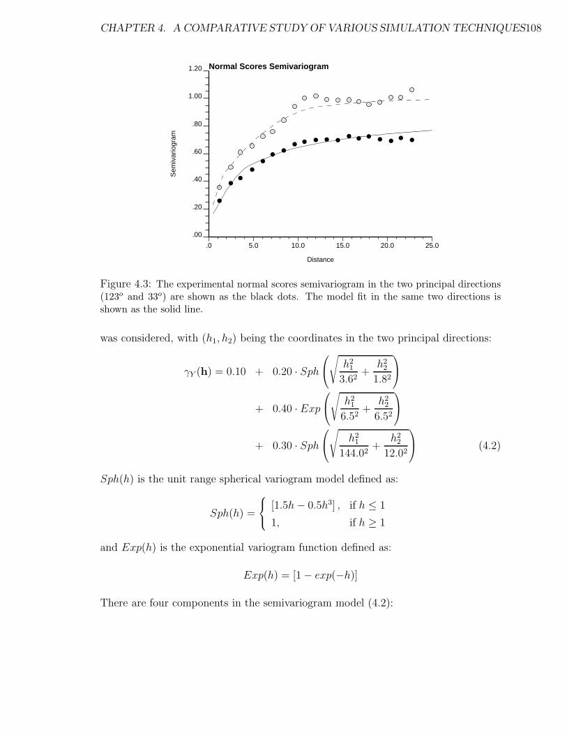
CHAPTER 4. A COMPARATIVE STUDY OF VARIOUS SIMULATION TECHNIQUES108
Sem
ivar
iogr
am
Distance
Normal Scores Semivariogram
.0 5.0 10.0 15.0 20.0 25.0
.00
.20
.40
.60
.80
1.00
1.20
Figure 4.3: The experimental normal scores semivariogram in the two principal directions(123o and 33o) are shown as the black dots. The model fit in the same two directions isshown as the solid line.
was considered, with (h1, h2) being the coordinates in the two principal directions:
γY (h) = 0.10 + 0.20 · Sph
√
h21
3.62+
h22
1.82
+ 0.40 · Exp
√
h21
6.52+
h22
6.52
+ 0.30 · Sph
√
h21
144.02+
h22
12.02
(4.2)
Sph(h) is the unit range spherical variogram model defined as:
Sph(h) =
[1.5h − 0.5h3] , if h ≤ 1
1, if h ≥ 1
and Exp(h) is the exponential variogram function defined as:
Exp(h) = [1 − exp(−h)]
There are four components in the semivariogram model (4.2):

CHAPTER 4. A COMPARATIVE STUDY OF VARIOUS SIMULATION TECHNIQUES109
1. an isotropic nugget effect that explains 10% of the total variability,
2. a short scale anisotropic spherical structure (the longer range of 3.6 is in the
major 123o direction and the shorter range of 1.8 is in the minor 33o direction)
that explains an additional 20% of the variability,
3. an isotropic long range exponential structure (the range parameter is 6.5, thus,
the effective range is 19.5) that explains 40% of the variability, and
4. finally, an anisotropic spherical structure to account for the zonal3 anisotropy
(the range parameter is 12.0 in the 33o direction and 144.0 in the 123o direction)
that explains the remaining 30% of the variability.
The stationary normal scores covariance CY (h) is related to the normal scores
variogram:
CY (h) = 1.0 − γY (h) (4.3)
and is used interchangeably in the following text.
The normal scores variogram or covariance is a specific two-point or bivariate
measure of the spatial variability of Berea. There is potentially much more bivariate
information, in the form of two-point indicator covariances. Beyond the bivariate
level there is multiple-point information in the form of multiple-point indicator co-
variances (see section 2.3.1) that could be considered to describe more completely the
spatial characteristics of the Berea image (Figure 4.1). The only case where the sole
normal scores covariance is sufficient to describe completely the spatial distribution
corresponds to a multivariate Gaussian model.
One test for bivariate Gaussianity consists of comparing the theoretically pre-
dicted indicator variograms, based on a bivariate Gaussian distribution model, to the
corresponding experimental indicator variograms (see [40, 91, 138]). A close corre-
spondence between the theoretical and experimental variograms would imply that the
data are bivariate Gaussian, hence the complete multivariate Gaussian assumption
3A zonal anisotropy relates to a variogram which reaches different sill values in different directions[90]. The range parameter of 144.0 is not reached within the boundary of the figure (40x40) andamounts to fitting a zonal anisotropy.
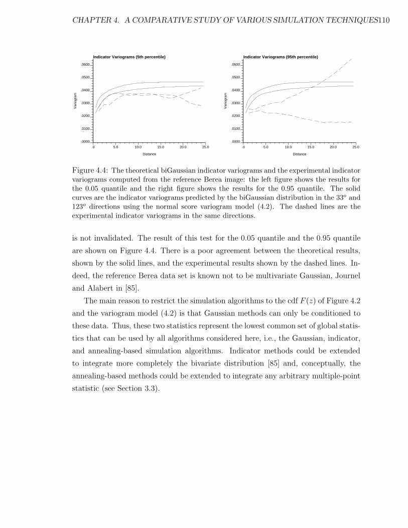
CHAPTER 4. A COMPARATIVE STUDY OF VARIOUS SIMULATION TECHNIQUES110
Var
iogr
am
Distance
Indicator Variograms (5th percentile)
.0 5.0 10.0 15.0 20.0 25.0
.0000
.0100
.0200
.0300
.0400
.0500
.0600
Var
iogr
am
Distance
Indicator Variograms (95th percentile)
.0 5.0 10.0 15.0 20.0 25.0
.0000
.0100
.0200
.0300
.0400
.0500
.0600
Figure 4.4: The theoretical biGaussian indicator variograms and the experimental indicatorvariograms computed from the reference Berea image: the left figure shows the results forthe 0.05 quantile and the right figure shows the results for the 0.95 quantile. The solidcurves are the indicator variograms predicted by the biGaussian distribution in the 33o and123o directions using the normal score variogram model (4.2). The dashed lines are theexperimental indicator variograms in the same directions.
is not invalidated. The result of this test for the 0.05 quantile and the 0.95 quantile
are shown on Figure 4.4. There is a poor agreement between the theoretical results,
shown by the solid lines, and the experimental results shown by the dashed lines. In-
deed, the reference Berea data set is known not to be multivariate Gaussian, Journel
and Alabert in [85].
The main reason to restrict the simulation algorithms to the cdf F (z) of Figure 4.2
and the variogram model (4.2) is that Gaussian methods can only be conditioned to
these data. Thus, these two statistics represent the lowest common set of global statis-
tics that can be used by all algorithms considered here, i.e., the Gaussian, indicator,
and annealing-based simulation algorithms. Indicator methods could be extended
to integrate more completely the bivariate distribution [85] and, conceptually, the
annealing-based methods could be extended to integrate any arbitrary multiple-point
statistic (see Section 3.3).

CHAPTER 4. A COMPARATIVE STUDY OF VARIOUS SIMULATION TECHNIQUES111
Flow D
irect
ion
Injector
Producer
Figure 4.5: Schematic illustration of the flow scenario.
Flow Scenario
The transfer function considered is a two-phase numerical flow simulation program
(Eclipse [48]). The 2-D grid of 40 by 40 point permeability values is associated to a
much larger horizontal grid of block horizontal permeabilities. This grid represents
one quarter of a five spot waterflooding production/injection scheme. The injector is
located in the lower left corner and the producer is located in the upper right corner,
see Figure 4.5. Thus, flow is perpendicular to the diagonal streak of low permeability
values aligned in the 123o direction in the lower left corner. All other flow properties,
except the block absolute permeabilities, have been held constant. The initially oil
saturated grid blocks are subjected to waterflooding and the fractional flow of oil
versus time4 is recorded. The three response variables retained are the time to achieve
breakthrough (5% water cut 5), the time to achieve a 95% water cut, and the time
required to recover 50% of the oil.
4The time unit is simply referred to as generic “time units” since the time is used only in arelative sense. For a constant rate injection scheme, as adopted in this problem, the actual timewould be directly related to the pore volumes injected.
5The water cut is the fractional flow rate of water. In cases, where only oil and water are flowingthe fractional flow of water is 1.0 minus the fractional flow of oil.

CHAPTER 4. A COMPARATIVE STUDY OF VARIOUS SIMULATION TECHNIQUES112
Fractional Flow of Oil versus Time
Time
Oil
Fra
ctio
n
0 10.0 20.0 30.0 40.0
.00
.20
.40
.60
.80
1.00
Figure 4.6: Fractional flow of oil for the reference Berea permeability distribution.
Figure 4.6 shows the reference waterflooding results, more precisely, the fractional
flow of oil versus time. The three reference response values are:
Time to reach 5% water cut = 4.178 time units
Time to reach 95% water cut = 29.956 time units
Time to recover 50% of the oil = 17.091 time units
The problem is to assess the uncertainty about these response variables using only
the univariate distribution of permeability values F (z) as shown on Figure 4.2, and
the normal scores semivariogram γY (h) shown on Figure 4.3 and modeled in equation
(4.2).
4.2 Stochastic Simulation and Output Uncertainty
The sequential Gaussian simulation (SGS) technique (see section 2.3.6), the sequen-
tial indicator simulation (SIS) technique (see section 2.3.7), and the annealing (SAS)
method (see section 2.5 and Chapter 3) have each been used to generate 100 uncon-
ditional (no local conditioning data) realizations of a square 40 by 40 grid the same
size as the reference Berea image of Figure 4.1. The acronyms SGS, SIS, and SAS
are used in the following text and figures to shorten the presentation.
CHAPTER 4. A COMPARATIVE STUDY OF VARIOUS SIMULATION TECHNIQUES113
The model distribution F (z) of 1600 values was used along with the normal scores
semivariogram model (4.2) as prior input information. Other implementation details
are given below:
Sequential Gaussian Simulation:
The sgsim program of GSLIB [40] was used to generate realizations with sequential
Gaussian simulation (SGS). A random path was followed in the sequential algorithm.
At each node the 24 closest previously simulated nodal values were retained for the
required simple kriging.
Each realization was generated in a reasonable 7.741 seconds of CPU time on a
DEC 5000 workstation (less than 15 minutes for the one hundred realizations). The
first four realizations, as shown on Figure 4.7, reproduce the important features of
the Berea sandstone. For example, the histogram of permeability, as visually appre-
ciated by the areal extent of different gray levels, is generally reproduced as is the
overall pattern of variability and anisotropy. These simulated realizations are consid-
ered plausible realizations of the Berea sandstone. The underlying model distribution
(cdf) was that of the 1600 reference values of Figure 4.2. However, statistical fluctu-
ations about this cdf model cause any one realization to have a different cdf. This
is illustrated on Figure 4.8 which shows a quantile-quantile plot with all 100 realiza-
tions. In average, the distribution of the SGS realizations is seen to reproduce the
reference distribution; however, there can be significant departures from the refer-
ence. These ergodic fluctuations contribute to the space of uncertainty defined by
SGS realizations. Section 4.3 considers how much of the uncertainty is due to these
ergodic fluctuations and how much is due to the higher order multivariate spatial
distribution.
The normal scores semivariogram of each realization also deviates from the model
semivariogram. This is illustrated on Figure 4.9 which shows the semivariogram,
for all 100 realizations, along the two principal directions. These fluctuations are
substantial and can not be removed by any conventional transformation procedure.
A more detailed look at ergodicity and the statistical fluctuations that can be expected
is given in Appendix B.

CHAPTER 4. A COMPARATIVE STUDY OF VARIOUS SIMULATION TECHNIQUES114
SGS Realization - One SGS Realization - Two
SGS Realization - Three SGS Realization - Four
Figure 4.7: The first four SGS realizations using the Berea permeability histogram andnormal scores semivariogram.

CHAPTER 4. A COMPARATIVE STUDY OF VARIOUS SIMULATION TECHNIQUES115
Q-Q Plot: SGS Realizations versus Reference
Reference
Sim
ulat
ed
0. 20. 40. 60. 80. 100. 120.
0.
20.
40.
60.
80.
100.
120.
Figure 4.8: A quantile-quantile plot of all 100 SGS realizations. Two identical distributionswould plot as a straight line at 45o-degrees (the gray line). In average, the distribution ofthe SGS realizations is close to the reference distribution.
Sequential Indicator Simulation:
The sisim program of GSLIB [40] was used to generate realizations with sequential
indicator simulation (SIS). A median IK approach (see section 2.3.7) was considered
with the stationary normal scores covariance model (4.2).
When the indicator thresholds or cutoffs are defined on p-quantiles qp the indicator
data i(u; qp) are the same regardless of the univariate distribution. For example,
choosing a first decile cutoff on the z-permeability data, zp=0.10 such that FZ(zp=0.10) =
0.10, yields the same indicator data as a first decile cutoff applied to the y-normal
scores data, yp=0.10 such that FY (yp=0.10) = 0.10, i.e.,
i(u; zp) = i(u; yp) when FZ(zp) = FY (yp)
Thus, the same results are obtained by performing the indicator simulation in the
normal space (with the nine deciles of the standard normal distribution) or directly
in the z-permeability space (with the nine deciles of the original Berea permeability

CHAPTER 4. A COMPARATIVE STUDY OF VARIOUS SIMULATION TECHNIQUES116
Normal Scores Semivariogram: 123 degrees
Distance
Sem
ivar
iogr
am
0 5.0 10.0 15.0 20.0 25.0
.00
.40
.80
1.20
1.60
Normal Scores Semivariogram: 33 degrees
Distance
Sem
ivar
iogr
am
0 5.0 10.0 15.0 20.0 25.0
.00
.40
.80
1.20
1.60
Figure 4.9: The normal scores semivariogram for all 100 SGS realizations in the twoprincipal directions. The model semivariogram is shown by the gray curve in the centerof the variogram cloud. The horizontal dashed line at a value of 1.0 represents the modelvariance. In average, the semivariogram of the SGS realizations is close to the modelsemivariogram.

CHAPTER 4. A COMPARATIVE STUDY OF VARIOUS SIMULATION TECHNIQUES117
distribution). To be consistent with SGS and annealing, and to make it straightfor-
ward to check reproduction of the stationary normal scores semivariogram, simulation
was performed in the normal space (with the nine standard normal deciles: -1.282,
-0.842, -0.524, -0.253, 0.000, 0.253, 0.524, 0.842, 1.282)
The normal scores semivariogram model (4.2) is adopted for all standardized in-
dicator semivariograms, and simple kriging was performed at all thresholds using the
24 closest previously simulated nodal values. At any particular location the data
configuration and the standardized semivariogram do not change from one cutoff to
the next. Therefore, at any one location the kriging weights do not change from one
cutoff to the next and only one kriging system need be solved with the same weights
applied to the different indicator data at all thresholds.
It took 12.12 seconds of CPU time on a DEC 5000 workstation to generate 1
realization (slightly over 20 minutes for the one hundred realizations). This is con-
sidered within practical limits. The first four realizations as shown on Figure 4.10,
are considered plausible realizations of the Berea permeability distribution since they
reasonably reproduce the histogram and general variability of the reference image.
Figure 4.11 shows a quantile-quantile plot of 100 realization cdf’s compared to the
reference distribution. In average, the distribution of a SIS realization is close to the
reference distribution. Once again the statistical (or ergodic) fluctuations are seen to
be significant (compare with the fluctuations obtained with the Gaussian method as
shown on Figure 4.8).
The semivariogram of each realization also fluctuates around the model semivari-
ogram. This is illustrated on Figure 4.12 which shows the semivariogram, for all 100
realizations, in the two principal directions. These fluctuations are significantly larger
than those observed with the SGS realizations, see Figure 4.9.
Annealing Simulation:
The sasim program (see Chapter 3, Appendix D, and GSLIB [40]) was used to gener-
ate realizations with the annealing (SAS) technique. The realizations were generated
in the normal space with the same distribution and semivarigoram as used by SGS
and SIS. The initial realization for each simulation was created by assigning the 1600

CHAPTER 4. A COMPARATIVE STUDY OF VARIOUS SIMULATION TECHNIQUES118
SIS Realization - One SIS Realization - Two
SIS Realization - Three SIS Realization - Four
Figure 4.10: The first four SIS realizations (generated with median indicator simulation)using the Berea permeability histogram and normal scores semivariogram.

CHAPTER 4. A COMPARATIVE STUDY OF VARIOUS SIMULATION TECHNIQUES119
Q-Q Plot: SIS Realizations versus Reference
Reference
Sim
ulat
ed
0. 20. 40. 60. 80. 100. 120.
0.
20.
40.
60.
80.
100.
120.
Figure 4.11: A quantile-quantile plot of all 100 SIS realizations. In average, the distributionof the SIS realizations is close to the reference distribution.
nodal values standard normal random deviates. Annealing was carried out with the
simulated annealing decision rule and the following objective function:
O =nh∑l=1
[γmodel(hl) − γrealization(hl)]2 (4.4)
The nh = 16 separation vectors h are defined by the offsets6 given on Table 4.1 and
graphically illustrated on Figure 4.13.
γmodel(hl) is the control or model variogram specified in (4.2), and γrealization(hl)
is the experimental semivariogram of the candidate realization.
It took 54.348 seconds of CPU time on a DEC 5000 workstation to perform 500,000
swaps and generate 1 realization when using a slow annealing schedule, see section
2.5, with parameters t0=1.0, λ = 0.5, Kmax = 160000, Kaccept = 16000, S = 5,
and ∆O = 0.000001, and running sasim until completion. Without changing the
annealing schedule, this time can be reduced by 50% by noticing that the objective
6It is relevant to state explicitly the offsets in the X and Y direction since this is the format usedby the sasim program.

CHAPTER 4. A COMPARATIVE STUDY OF VARIOUS SIMULATION TECHNIQUES120
Normal Scores Semivariogram: 123 degrees
Distance
Sem
ivar
iogr
am
0 5.0 10.0 15.0 20.0 25.0
.00
.40
.80
1.20
1.60
Normal Scores Semivariogram: 33 degrees
Distance
Sem
ivar
iogr
am
0 5.0 10.0 15.0 20.0 25.0
.00
.40
.80
1.20
1.60
Figure 4.12: The normal scores semivariogram for all 100 SIS realizations in the twoprincipal directions. The model semivariogram is shown by the gray curve in the center ofthe variogram cloud.

CHAPTER 4. A COMPARATIVE STUDY OF VARIOUS SIMULATION TECHNIQUES121
Lag Number X (horizontal offset) Y (vertical offset)1 1 02 0 13 1 14 1 -15 2 06 0 27 2 28 2 -29 2 110 1 211 1 -212 2 -113 3 -214 6 -415 2 316 4 6
Table 4.1: The lag vectors used with annealing to generate unconditional simulations withthe Berea distribution and normal scores semivariogram. These vectors are graphicallyillustrated on Figure 4.13.

CHAPTER 4. A COMPARATIVE STUDY OF VARIOUS SIMULATION TECHNIQUES122
1
2 3
4
5
6 7
8
9
10
11
12
13
14
15
16
Figure 4.13: The lag vectors used to generate unconditional realizations of Berea. The lagnumbers correspond to those given on Table 4.1.
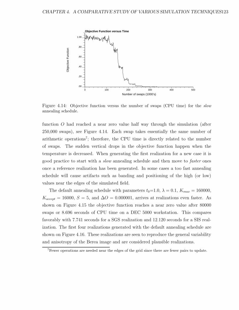
CHAPTER 4. A COMPARATIVE STUDY OF VARIOUS SIMULATION TECHNIQUES123
Objective Function versus Time
Number of swaps (1000’s)
Obj
ectiv
e F
unct
ion
0 100 200 300 400 500
.00
.20
.40
.60
.80
1.00
Figure 4.14: Objective function versus the number of swaps (CPU time) for the slowannealing schedule.
function O had reached a near zero value half way through the simulation (after
250,000 swaps), see Figure 4.14. Each swap takes essentially the same number of
arithmetic operations7; therefore, the CPU time is directly related to the number
of swaps. The sudden vertical drops in the objective function happen when the
temperature is decreased. When generating the first realization for a new case it is
good practice to start with a slow annealing schedule and then move to faster ones
once a reference realization has been generated. In some cases a too fast annealing
schedule will cause artifacts such as banding and positioning of the high (or low)
values near the edges of the simulated field.
The default annealing schedule with parameters t0=1.0, λ = 0.1, Kmax = 160000,
Kaccept = 16000, S = 5, and ∆O = 0.000001, arrives at realizations even faster. As
shown on Figure 4.15 the objective function reaches a near zero value after 80000
swaps or 8.696 seconds of CPU time on a DEC 5000 workstation. This compares
favorably with 7.741 seconds for a SGS realization and 12.120 seconds for a SIS real-
ization. The first four realizations generated with the default annealing schedule are
shown on Figure 4.16. These realizations are seen to reproduce the general variability
and anisotropy of the Berea image and are considered plausible realizations.
7Fewer operations are needed near the edges of the grid since there are fewer pairs to update.

CHAPTER 4. A COMPARATIVE STUDY OF VARIOUS SIMULATION TECHNIQUES124
Objective Function versus Time
Number of swaps (1000’s)
Obj
ectiv
e F
unct
ion
0 100 200 300 400 500
.00
.20
.40
.60
.80
1.00
Figure 4.15: Objective function versus the number of swaps (CPU time) for the fastannealing schedule.
Figure 4.17 shows a quantile-quantile plot of all 100 realization cdf’s compared
to the reference distribution. Each of the annealing realization cdf’s is seen to be
very close to the reference distribution since the initial cdf is not changed by the
annealing/perturbation process. The 1600 nodal values are each initially assigned
by randomly drawing from a standard normal distribution. The fluctuations on Fig-
ure 4.17 are the result of this drawing. Compare with the fluctuations obtained with
SGS and SIS shown on Figures 4.8 and 4.11.
The semivariogram of each realization deviates from the model semivariogram to
a much lesser degree than either SGS or SIS. This is illustrated on Figure 4.18 (to
be compared with Figures 4.9 and 4.12) which shows the semivariogram, for all 100
realizations, in the two principal directions. The fluctuations beyond 7-8 distance
units arise because the corresponding model semivariogram values do not enter the
objective function.
In most practical situations the model statistics (univariate distribution and semi-
variogram) have been inferred from a limited number of sample data; thus, one expects
a certain amount of sampling uncertainty. In such cases, the tight control provided
by the SAS realizations may not be desireable.

CHAPTER 4. A COMPARATIVE STUDY OF VARIOUS SIMULATION TECHNIQUES125
SAS Realization - One SAS Realization - Two
SAS Realization - Three SAS Realization - Four
Figure 4.16: The first four annealing realizations using the Berea permeability histogramand normal scores semivariogram.

CHAPTER 4. A COMPARATIVE STUDY OF VARIOUS SIMULATION TECHNIQUES126
Q-Q Plot: SAS Realizations versus Reference
Reference
Sim
ulat
ed
0. 20. 40. 60. 80. 100. 120.
0.
20.
40.
60.
80.
100.
120.
Figure 4.17: A quantile-quantile plot of all 100 annealing realizations. The distribution ofeach annealing realization is close to the reference distribution.
Practical Considerations in Choosing Annealing Simulation Parameters:
The annealing-based simulated realizations shown on Figure 4.16 appear reasonable
when compared to the SGS and SIS realizations shown on Figures 4.7 and 4.10.
Depending on the objective function and the annealing schedule it is possible to get
unreasonable realizations. The following empirical rules can be followed to avoid such
unreasonable results:
1. In general, the separation vectors chosen to enter the objective function should
cover a compact volumetric extent as illustrated on Figure 4.13 (in this case,
the two lags at longer distances help the results and do not lead to artifacts).
For example, choosing four lags that are not contiguous, i.e., (2,3), (4,6), (3,-
2), (6,-4), (shown on Figure 4.19) will yield realizations like those shown on
Figure 4.20. The objective function can be lowered to zero with realizations
showing a checkerboard appearance. A checkerboard is perfectly continuous for
every second lag.

CHAPTER 4. A COMPARATIVE STUDY OF VARIOUS SIMULATION TECHNIQUES127
Normal Scores Semivariogram: 123 degrees
Distance
Sem
ivar
iogr
am
0 5.0 10.0 15.0 20.0 25.0
.00
.40
.80
1.20
1.60
Normal Scores Semivariogram: 33 degrees
Distance
Sem
ivar
iogr
am
0 5.0 10.0 15.0 20.0 25.0
.00
.40
.80
1.20
1.60
Figure 4.18: The normal scores semivariogram for all 100 annealing realizations in the twoprincipal directions. The model semivariogram is shown by the gray curve in the center ofthe variogram cloud.

CHAPTER 4. A COMPARATIVE STUDY OF VARIOUS SIMULATION TECHNIQUES128
1
2
3
4
Figure 4.19: The four lag vectors used to generate unconditional realizations with artifactcheckerboard appearance. The lag numbers correspond to offsets (2,3), (4,6), (3,-2), (6,-4).This figure is to be compared to Figure 4.13 which does not lead to any artifacts.

CHAPTER 4. A COMPARATIVE STUDY OF VARIOUS SIMULATION TECHNIQUES129
SAS with four lags SAS with four lags
Figure 4.20: Two SAS realizations using the offset pairs of (2,3), (4,6), (3,-2), (6,-4) shownin Figure 4.19. The separation of the pairs leads to an unreasonable checkerboard appear-ance.
2. To reduce the required CPU time it is tempting to reduce quickly the temper-
ature in the annealing schedule. In some cases the temperature can be lowered
quickly with no consequent artifacts. In this case, if the temperature is set to
zero each realization is generated in 10000 swaps or 1.587 seconds on a DEC
5000. Two realizations are shown on Figure 4.21 with no apparent artifacts;
however, in general a too fast annealing schedule will cause a lack of convergence
and poor quality realizations. The default annealing schedule documented in
section 2.5 and coded in sasim is typically slow enough to lead to reasonable
realizations.
Flow Simulation Results:
Flow simulation, with a constant pressure drop between the injector and producer,
was performed on each of the 3 · 100 = 300 realizations. On average, it took 281
seconds on a DEC 5000 for each flow simulation. Recall that it took 7.74, 12.12, and
8.70 DEC 5000 seconds to generate a realization with sequential Gaussian, sequential

CHAPTER 4. A COMPARATIVE STUDY OF VARIOUS SIMULATION TECHNIQUES130
SAS with Temperature=zero SAS with Temperature=zero
Figure 4.21: Two SAS realizations with the temperature set to zero. These realizationsappear quite reasonable.
indicator, and annealing techniques.
The space of output uncertainty defined by each method is characterized by the
distribution (histogram) of each of the three output response variables. The his-
tograms for time8 to achieve breakthrough, the time to achieve a water cut of 95%,
and the time required to recover 50% of the oil, are shown on Figures 4.22, 4.23, and
4.24 for sequential Gaussian, sequential indicator, and annealing simulation, respec-
tively.
All simulated output distributions contain the true reference value as obtained
from the reference Berea image: the reference black dots on Figures 4.22, 4.23, and
4.24 are within the 95% probability intervals. In all cases the center (mean or median)
of the output distributions is higher than the reference value. The breakthrough time
and oil recovery is faster with the reference image than the average predicted by any
of the three simulation algorithms.
This systematic difference is explained by particular features of the reference Berea
image of Figure 4.1. The low permeability near the injector and the high permeability
8For this example, the units of time are not relevant since the same response variable is beingconsidered in all cases. The time is real time and not pore volumes injected.

CHAPTER 4. A COMPARATIVE STUDY OF VARIOUS SIMULATION TECHNIQUES131
Fre
quen
cy
.0 2.0 4.0 6.0 8.0 10.0
.000
.040
.080
.120
.160
Response One: unconditional SGS
True = 4.178
mean 4.8717std. dev. .8532
coef. of var .1751
maximum 7.2928upper quartile 5.4651
median 4.6694lower quartile 4.2416
minimum 3.3951
Fre
quen
cy
20.0 30.0 40.0 50.0 60.0
.000
.040
.080
.120
Response Two: unconditional SGS
True = 29.956
mean 33.0602std. dev. 4.4479
coef. of var .1345
maximum 44.7830upper quartile 36.0873
median 31.9523lower quartile 30.0914
minimum 25.2867
Fre
quen
cy
10.0 15.0 20.0 25.0 30.0
.000
.040
.080
.120Response Three: unconditional SGS
True = 17.091
mean 18.7598std. dev. 2.3542
coef. of var .1255
maximum 24.8604upper quartile 20.3861
median 18.3413lower quartile 17.0085
minimum 14.4716
Figure 4.22: The simulated output distributions generated by the unconditional sequentialGaussian realizations. The upper histogram is for the time to achieve 5% water cut, themiddle histogram is for the time to achieve a 95% water cut, and the lower histogram isfor the time to recover 50% of the oil. The black dot in the box plot below each histogramis the true value obtained from the reference image, the three vertical lines are the 0.025quantile, the median (0.5 quantile), and the 0.975 quantile of the output distribution.

CHAPTER 4. A COMPARATIVE STUDY OF VARIOUS SIMULATION TECHNIQUES132
Fre
quen
cy
.0 2.0 4.0 6.0 8.0 10.0
.000
.040
.080
.120
.160
Response One: unconditional SIS
True = 4.178
mean 4.9474std. dev. .8028
coef. of var .1623
maximum 7.2935upper quartile 5.4046
median 4.7717lower quartile 4.3191
minimum 3.5474
Fre
quen
cy
20.0 30.0 40.0 50.0 60.0
.000
.040
.080
.120
Response Two: unconditional SIS
True = 29.956
mean 33.6503std. dev. 4.1778
coef. of var .1242
maximum 46.2240upper quartile 36.2371
median 32.9109lower quartile 30.2623
minimum 26.0475
Fre
quen
cy
10.0 15.0 20.0 25.0 30.0
.000
.040
.080
.120
Response Three: unconditional SIS
True = 17.091
mean 19.1450std. dev. 2.2606
coef. of var .1181
maximum 25.8093upper quartile 20.2333
median 18.8895lower quartile 17.4985
minimum 14.7144
Figure 4.23: The simulated output distributions generated by the unconditional sequentialindicator realizations. The upper histogram is for the time to achieve 5% water cut, themiddle histogram is for the time to achieve a 95% water cut, and the lower histogram isfor the time to recover 50% of the oil. The black dot in the box plot below each histogramis the true value obtained from the reference image, the three vertical lines are the 0.025quantile, the median (0.5 quantile), and the 0.975 quantile of the output distribution.

CHAPTER 4. A COMPARATIVE STUDY OF VARIOUS SIMULATION TECHNIQUES133
Fre
quen
cy
.0 2.0 4.0 6.0 8.0 10.0
.000
.040
.080
.120
Response One: unconditional SAS
True = 4.178
mean 5.1005std. dev. 1.0397
coef. of var .2038
maximum 7.6889upper quartile 5.7904
median 5.1028lower quartile 4.1890
minimum 3.2988
Fre
quen
cy
20.0 30.0 40.0 50.0 60.0
.0000
.0100
.0200
.0300
.0400
.0500
.0600
.0700
.0800Response Two: unconditional SAS
True = 29.956
mean 34.5353std. dev. 5.7947
coef. of var .1678
maximum 48.7835upper quartile 38.7852
median 34.2986lower quartile 29.7469
minimum 24.6263
Fre
quen
cy
10.0 15.0 20.0 25.0 30.0
.000
.020
.040
.060
.080
Response Three: unconditional SAS
True = 17.091
mean 19.6551std. dev. 3.2340
coef. of var .1645
maximum 27.9956upper quartile 21.9916
median 19.3641lower quartile 17.0208
minimum 14.3032
Figure 4.24: The simulated output distributions generated by the unconditional annealingrealizations. The upper histogram is for the time to achieve 5% water cut, the middlehistogram is for the time to achieve a 95% water cut, and the lower histogram is for thetime to recover 50% of the oil. The black dot in the box plot below each histogram is thetrue value obtained from the reference image, the three vertical lines are the 0.025 quantile,the median (0.5 quantile), and the 0.975 quantile of the output distribution.

CHAPTER 4. A COMPARATIVE STUDY OF VARIOUS SIMULATION TECHNIQUES134
SGS realization with short time (3.40)
Injector
ProducerSGS realization with long time (7.29)
Injector
Producer
Figure 4.25: The SGS realizations that yield the shortest and the longest time to reach awater cut of 5%.
near the producer are factors. Another important factor is the continuity perpendic-
ular to the flow direction. Intuitively, one would think that the continuity between
the wells (parallel to the flow direction) is the most important factor for early break-
through. However, the wells are separated by 5 times the variogram range in that
direction and there is virtually no possibility for a direct flow path between the wells.
Continuity perpendicular to the pressure gradient as present in Berea allows a more
direct and less tortuous path from the injector to producer. This is confirmed by
visually examining the SGS, SIS, and SAS realizations that generate the shortest
“time to reach a 5% water cut” shown on the left of Figures 4.25, 4.26, and 4.27.
For all three simulation algorithms the short time cases are those where the overall
permeability is high and connected in the direction perpendicular to flow.
Figures 4.25, 4.26, and 4.27 also show the the realizations that give the longest
“time to reach a 5% water cut”. The long time realizations are characterized by overall
low permeability and a lack of continuity either between the wells or perpendicular
to the flow direction.

CHAPTER 4. A COMPARATIVE STUDY OF VARIOUS SIMULATION TECHNIQUES135
SIS realization with short time (3.55)
Injector
ProducerSIS realization with long time (7.29)
Injector
Producer
Figure 4.26: The SIS realizations that yield the shortest and the longest time to reach awater cut of 5%.
SAS realization with short time (3.29)
Injector
ProducerSAS realization with long time (7.69)
Injector
Producer
Figure 4.27: The SAS realizations that yield the shortest and the longest time to reach awater cut of 5%.

CHAPTER 4. A COMPARATIVE STUDY OF VARIOUS SIMULATION TECHNIQUES136
Response Variable Technique 95% Probability Intervalq0.025 q0.975 width
Time to reach 5% SGS 3.60 6.88 3.28SIS 3.67 6.98 3.31SAS 3.49 7.25 3.76
Time to reach 95% SGS 26.15 42.77 16.62SIS 26.78 43.71 16.93SAS 24.78 46.75 21.97
Time to recover 50% SGS 15.43 24.04 8.61SIS 15.79 25.39 9.60SAS 14.57 26.52 11.95
Table 4.2: Summary of output response for SGS, SIS, and SAS realizations.
The space of output uncertainty generated by SGS, SIS, and SAS may be sum-
marized by the 95% probability intervals of the three response variables that they
generate. The 95% probability interval is bound by the 2.5% quantile (q0.025) and
the 97.5% quantile (q0.975). The width of the 95% probability interval is defined as
q0.975 − q0.025. Table 4.2 gives the 95% probability interval for the output response
distributions generated by the SGS, SIS, and SAS simulated realizations.
In all cases the width of the 95% probability interval is largest for the annealing
(SAS) realizations. This was not expected since the Gaussian and indicator input im-
ages showed significantly more ergodic fluctuations (see Figures 4.8 and 4.11 versus
4.17 and also Figures 4.9 and 4.12 versus 4.18). Moreover, the annealing realizations
are indirectly the result of an optimization procedure whereas the Gaussian and indi-
cator realizations are generated by more traditional RF-based simulation procedures.
These facts would have a-priori led one to believe that annealing would generate a
smaller space of output uncertainty.
The SGS and SIS realizations clearly reflect more univariate and bivariate vari-
ability; however, the flow simulator response is a complex multivariate characteristic.

CHAPTER 4. A COMPARATIVE STUDY OF VARIOUS SIMULATION TECHNIQUES137
There is no theoretical or empirical relation between input uncertainty at the uni-
variate and bivariate level and output uncertainty. By construction SGS realizations
have a multivariate Gaussian distribution. It is also known that these Gaussian im-
ages have maximum entropy (see Appendix C) which may lead to realizations with
too similar flow characteristics (i.e., a smaller space of output uncertainty).
The implicit multivariate distribution of annealing realizations is the result of
many implementation decisions (see Chapter 3) and the components entering the
objective function. The result of Table 4.2 allows the conjecture that departure from
a multivariate Gaussian distribution and its maximum entropy feature in general
leads to a larger sampled space of output uncertainty.
4.3 Uncertainty due to Ergodic Fluctuations
All three simulation algorithms generate realizations {z(l)(u),u ∈ A} whose cdf
F (l)(z) and variogram γ(l)(h) deviate from the corresponding model parameters F (z)
and γ(h). These deviations, referred to as ergodic fluctuations, lead to a larger space
of input uncertainty, i.e., realizations that honor exactly the model cdf and variogram
can be considered as a subset of all the realizations. The ergodic fluctuations of the
conventional RF-based SGS and SIS algorithms were significantly more pronounced
than those of the annealing-based algorithm. The larger the space of possible out-
comes the more conservative assessment of output uncertainty; thus, at the univariate
and bivariate level the SGS and SIS realizations present a larger space of uncertainty.
There are two relevant questions related to ergodic fluctuations: 1) how much fluc-
tuation is acceptable?, and 2) how much is the space of output uncertainty expanded
by these fluctuations? Some fluctuations are acceptable and desirable since the model
statistics are typically affected by sampling fluctuations. Note that a higher order
model of uncertainty for the model parameters (F (z) and γY (h)) would be needed to
rigorously evaluate how much fluctuation is acceptable.
In many applications, the model statistics are inferred from sparse samples and

CHAPTER 4. A COMPARATIVE STUDY OF VARIOUS SIMULATION TECHNIQUES138
cannot be considered as perfectly known. Therefore, deviations from the model statis-
tics are desirable because they address a real aspect of the inherent uncertainty. Al-
though ergodic fluctuations have the same impact on the output response variables
as uncertain or randomized input model parameters; the source of the variability is
quite different. Ergodic fluctuations arise only because the physical size of the domain
being simulated is not infinite (see Appendix B). All simulation algorithms, regardless
of the ergodic fluctuations, implicitly consider that the model statistics are perfectly
known.
A worthwhile goal would be to introduce explicitly the uncertainty in the model
statistics, e.g., in some parameters of the cdf F (z) and variogram γ(h). A model
of uncertainty in these parameters could be constructed and Monte Carlo drawings
from these models would yield the parameters to be used for each realization. Thus,
fluctuations from the model parameters would be explicitly controlled. This approach
has not been considered in this dissertation and may be an interesting topic of future
research.
The other question regarding ergodic fluctuations which has been investigated
in this section is “how much is the output space of uncertainty expanded by these
fluctuations?”. To address this question one needs a subset of realizations that exactly
honor the conditioning statistics.
One idea would be to generate many realizations and keep only those that honor
the model distribution F (z) and model variogram γY (h) with some strict tolerance.
This idea was not pursued since a prohibitively large number of realizations would
have to be created to find enough that simultaneously honor F (z) and γY (h). Rather
than generate new realizations, a univariate graphical transformation procedure (see
[90], p. 478 and [40], p. 191) was used to transform the 100 SGS and the 100
SIS realizations to exactly match the model distribution F (z). Thus, the ergodic
fluctuations of F (z) can be isolated while leaving the fluctuations in the variogram9.
The transform is achieved by replacing each z-value of a particular image by a
9There is no such straightforward bivariate transform to remove fluctuations from a referencecovariance or variogram.

CHAPTER 4. A COMPARATIVE STUDY OF VARIOUS SIMULATION TECHNIQUES139
rank-preserving graphical transform, i.e,
z = F−1(F (l)(z′)) (4.5)
where F−1(·) is the inverse of the reference (model) distribution, F (l)(·) is the distri-
bution for simulation (l), z′ is a simulated value from F (l)(z), and z is the transformed
value.
The results of this histogram identification are illustrated on Figure 4.28 where
the third and fourth SGS realizations (the bottom of Figure 4.7) have been trans-
formed to reproduce exactly the distribution of Figure 4.2. The transform does not
change the spatial arrangement of high and low permeabilities; only the magnitude is
changed so that the reference histogram is reproduced. For example, the permeability
distribution shown on the upper left of Figure 4.28 had a too large proportion of low
permeability (light colored pixels). These low permeabilities have been rescaled to
obtain the distribution shown on the upper right of Figure 4.28 which has the correct
proportion of high and low permeability. Similarly, the distribution shown on the
lower left of Figure 4.28 had a too large proportion of high permeability (dark colored
pixels). The rescaled distribution shown on the lower right has the correct proportion
of each permeability type.
The univariate distribution of all 100 SGS and 100 SIS realizations F (l)(z) have
been transformed to identify the reference distribution F (z). The numerical flow
simulation was repeated to obtain the new response values. The histograms of output
response values are shown on Figures 4.29 and 4.30. The space of output uncertainty
generated before and after the univariate transformation is summarized by the 95%
probability intervals of the three response variables shown on Table 4.3.
In general, the space of uncertainty, as measured by the width of the 95% proba-
bility interval, decreases when the ergodic fluctuations in the histogram are removed.
The width of the 95% probability interval has been reduced by an average of 9% for
the SGS realizations and by an average of 25% reduction for the SIS realizations. The
larger reduction in the case of the SIS realizations is expected since the original 100
realizations showed significantly more ergodic fluctuations in the histogram than the
SGS realizations (compare Figures 4.8 and 4.11).

CHAPTER 4. A COMPARATIVE STUDY OF VARIOUS SIMULATION TECHNIQUES140
SGS Realization - Three SGS Realization - Transformed Three
SGS Realization - Four SGS Realization - Transformed Four
Figure 4.28: Two SGS realizations (the third and fourth realizations on Figure 4.7) beforeand after being transformed to identify the reference Berea permeability histogram.
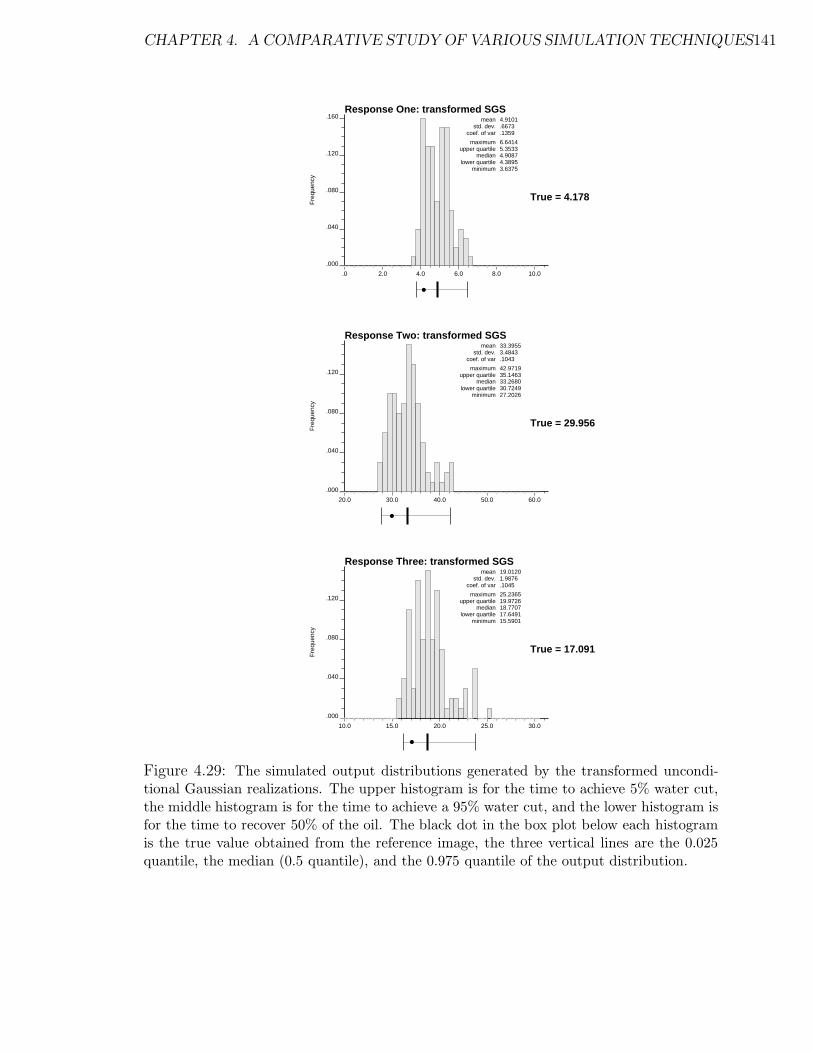
CHAPTER 4. A COMPARATIVE STUDY OF VARIOUS SIMULATION TECHNIQUES141
Fre
quen
cy
.0 2.0 4.0 6.0 8.0 10.0
.000
.040
.080
.120
.160Response One: transformed SGS
True = 4.178
mean 4.9101std. dev. .6673
coef. of var .1359
maximum 6.6414upper quartile 5.3533
median 4.9087lower quartile 4.3895
minimum 3.6375
Fre
quen
cy
20.0 30.0 40.0 50.0 60.0
.000
.040
.080
.120
Response Two: transformed SGS
True = 29.956
mean 33.3955std. dev. 3.4843
coef. of var .1043
maximum 42.9719upper quartile 35.1463
median 33.2680lower quartile 30.7249
minimum 27.2026
Fre
quen
cy
10.0 15.0 20.0 25.0 30.0
.000
.040
.080
.120
Response Three: transformed SGS
True = 17.091
mean 19.0120std. dev. 1.9876
coef. of var .1045
maximum 25.2365upper quartile 19.9726
median 18.7707lower quartile 17.6491
minimum 15.5901
Figure 4.29: The simulated output distributions generated by the transformed uncondi-tional Gaussian realizations. The upper histogram is for the time to achieve 5% water cut,the middle histogram is for the time to achieve a 95% water cut, and the lower histogram isfor the time to recover 50% of the oil. The black dot in the box plot below each histogramis the true value obtained from the reference image, the three vertical lines are the 0.025quantile, the median (0.5 quantile), and the 0.975 quantile of the output distribution.

CHAPTER 4. A COMPARATIVE STUDY OF VARIOUS SIMULATION TECHNIQUES142
Fre
quen
cy
.0 2.0 4.0 6.0 8.0 10.0
.000
.040
.080
.120
.160
Response One: transformed SIS
True = 4.178
mean 4.7795std. dev. .6098
coef. of var .1276
maximum 6.5578upper quartile 5.2285
median 4.7133lower quartile 4.3086
minimum 3.5482
Fre
quen
cy
20.0 30.0 40.0 50.0 60.0
.000
.040
.080
.120
.160
Response Two: transformed SIS
True = 29.956
mean 32.5745std. dev. 3.0376
coef. of var .0933
maximum 42.3085upper quartile 34.7588
median 32.0443lower quartile 30.4497
minimum 26.4870
Fre
quen
cy
10.0 15.0 20.0 25.0 30.0
.000
.040
.080
.120
Response Three: transformed SIS
True = 17.091
mean 18.5452std. dev. 1.7229
coef. of var .0929
maximum 23.4879upper quartile 19.7219
median 18.2691lower quartile 17.1133
minimum 15.0275
Figure 4.30: The simulated output distributions generated by the transformed uncondi-tional indicator realizations. The upper histogram is for the time to achieve 5% water cut,the middle histogram is for the time to achieve a 95% water cut, and the lower histogram isfor the time to recover 50% of the oil. The black dot in the box plot below each histogramis the true value obtained from the reference image, the three vertical lines are the 0.025quantile, the median (0.5 quantile), and the 0.975 quantile of the output distribution.

CHAPTER 4. A COMPARATIVE STUDY OF VARIOUS SIMULATION TECHNIQUES143
Response Variable Technique 95% Probability Interval % reductionq0.025 q0.975 width
Time to reach 5% SGS (before) 3.60 6.88 3.28SGS (after) 3.80 6.98 3.18 -3%SIS (before) 3.67 6.98 3.31SIS (after) 3.69 6.48 2.79 -16%
Time to reach 95% SGS (before) 26.15 42.77 16.62SGS (after) 27.85 42.37 14.52 -13%SIS (before) 26.78 43.71 16.93SIS (after) 27.06 38.88 11.82 -30%
Time to recover 50% SGS (before) 15.43 24.04 8.61SGS (after) 16.23 23.83 7.60 -11%SIS (before) 15.79 25.39 9.60SIS (after) 15.54 22.48 6.94 -28%
Table 4.3: Summary of SGS and SIS output response results before and after removingergodic fluctuations in the cdf.

CHAPTER 4. A COMPARATIVE STUDY OF VARIOUS SIMULATION TECHNIQUES144
The ergodic fluctuations of the SAS (annealing) realizations were minimal (see
Figure 4.17) and removing them would have yielded the same results as those shown
on Table 4.2. Although the output uncertainty is significantly higher for the SAS
realizations, this uncertainty is due to the multivariate (1600-variate) distribution
well beyond the variability controlled by the one and two-point distribution.
In practice, the output uncertainty is constrained by more than just a cdf and
variogram model. The permeability (and other rock properties) are known at the
well locations. The next section investigates how conditioning to local data affects
the output uncertainty.
4.4 Conditioning to Local Data
The realizations generated up until now have not considered any local conditioning
data z(uα), α = 1, . . . , n, so that the visual appearance and output uncertainty are
the result of only the implicit RF models. In practice, there are always some local
conditioning data; in particular, the petrophysical properties are typically known at
the well locations through direct measurements or interpretation of various well log
responses.
Sequential Gaussian, sequential indicator, and annealing simulation as documented
in section 2.2 have been repeated with two local conditioning data as taken from the
reference map of Figure 4.1: the permeability at the injector (45.0 md) and the per-
meability at the producer (88.0 md). In all three cases the conditioning is achieved
by fixing these two nodal values at the start of the simulation procedure. In the case
of sequential Gaussian and sequential indicator simulation these two data are used
to condition all remaining 1598 nodes. In the case of annealing these two data are
left unperturbed during the entire annealing procedure. Four conditional realizations
for SGS, SIS, and SAS are shown on Figures 4.31, 4.32, and 4.33 respectively. In all
cases the permeability in the upper right corner is higher (due to the producing well
permeability of 88 md) and the permeability in the lower left corner is lower (due to
the injecting well permeability of 45 md).

CHAPTER 4. A COMPARATIVE STUDY OF VARIOUS SIMULATION TECHNIQUES145
The flow simulation was repeated with the 3 · 100 = 300 realizations. The his-
tograms of flow response variables are shown on Figures 4.34, 4.35, and 4.36. The
results for all runs, including these conditional realizations, are shown on Table 4.4.
It appears that adding these two conditioning data has not decreased the space of
uncertainty. Two data are not sufficient to constrain the spatial distribution to an
amount noticeable by the transfer function used here (flow simulator).
4.5 Summary of the Results
The primary result of this chapter is that the annealing-based simulation results
appear to fulfill the requirements of a good simulation technique. That is,
• Plausible realizations were generated in a reasonable amount of computer time.
It took 8.696 seconds of CPU time on a DEC 5000 workstation for an SAS
realization. This compares with 7.741 seconds for a SGS realization and 12.120
seconds for a SIS realization.
• All of the input data were honored. The univariate distribution and the vari-
ogram were honored more exactly than either the SGS or the SIS realizations
(see Figure 4.17 versus 4.8 and 4.11 and also Figure 4.18 versus 4.9 and 4.12).
This is not necessarily an advantage since the ergodic fluctuations of SGS and
SIS could be considered as accounting for sampling uncertainty in the model
statistics.
• Finally, the annealing-based realizations seem to generate a space of output
uncertainty comparable to both SGS and SIS. In fact, in all cases the SAS
realizations generated a slightly larger space of uncertainty (see Table 4.4).

CHAPTER 4. A COMPARATIVE STUDY OF VARIOUS SIMULATION TECHNIQUES146
Case Time to reach 5% Time to reach 95% Time for 50% recoveryq0.025 q0.975 width q0.025 q0.975 width q0.025 q0.975 width
Unconditional SimulationsSGS 3.60 6.88 3.28 26.15 42.77 16.62 15.43 24.04 8.61SIS 3.67 6.98 3.31 26.78 43.71 16.93 15.79 25.39 9.60SAS 3.49 7.25 3.76 24.78 46.75 21.97 14.57 26.52 11.95
Transformed Unconditional SimulationsSGS 3.80 6.98 3.18 27.85 42.37 14.52 16.23 23.83 7.60SIS 3.69 6.48 2.79 27.06 38.88 11.82 15.54 22.48 6.94
Conditional SimulationsSGS 3.58 6.84 3.26 26.06 42.94 16.88 14.80 23.96 9.16SIS 3.66 7.27 3.61 26.33 45.32 18.99 15.69 26.04 10.35SAS 3.49 7.47 3.98 25.59 48.59 23.00 14.66 28.30 13.64
Table 4.4: Summary of all output response values. The unconditional realizations consideronly a distribution model F (z) and a variogram model γY (h). The transformed resultscorrespond to the same unconditional SGS and SIS results with the ergodic fluctuations inthe cdf F (l)(z) removed. The conditional results consider two local conditioning data; oneat each well. The output uncertainty generated by each simulation method is the width ofthe 95% probability interval (q0.975 − q0.025).

CHAPTER 4. A COMPARATIVE STUDY OF VARIOUS SIMULATION TECHNIQUES147
SGS Conditional Realization - One SGS Conditional Realization - Two
SGS Conditional Realization - Three SGS Conditional Realization - Four
Figure 4.31: The first four sequential Gaussian realizations using the Berea permeabilityhistogram, and normal scores semivariogram model, and two conditioning data.

CHAPTER 4. A COMPARATIVE STUDY OF VARIOUS SIMULATION TECHNIQUES148
SIS Conditional Realization - One SIS Conditional Realization - Two
SIS Conditional Realization - Three SIS Conditional Realization - Four
Figure 4.32: The first four sequential indicator realizations using the Berea permeabilityhistogram, and normal scores semivariogram model, and two conditioning data.

CHAPTER 4. A COMPARATIVE STUDY OF VARIOUS SIMULATION TECHNIQUES149
SAS Conditional Realization - One SAS Conditional Realization - Three
SAS Conditional Realization - Three SAS Conditional Realization - Four
Figure 4.33: The first four annealing realizations using the Berea permeability histogram,and normal scores semivariogram model, and two conditioning data.

CHAPTER 4. A COMPARATIVE STUDY OF VARIOUS SIMULATION TECHNIQUES150
Fre
quen
cy
.0 2.0 4.0 6.0 8.0 10.0
.000
.040
.080
.120
Response One: conditional SGS
True = 4.178
mean 4.9582std. dev. .8605
coef. of var .1736
maximum 8.7430upper quartile 5.3872
median 4.8200lower quartile 4.3492
minimum 3.4646
Fre
quen
cy
20.0 30.0 40.0 50.0 60.0
.000
.020
.040
.060
.080
.100
Response Two: conditional SGS
True = 29.956
mean 33.2936std. dev. 4.4735
coef. of var .1344
maximum 48.7133upper quartile 35.4617
median 32.9098lower quartile 30.1443
minimum 25.7926
Fre
quen
cy
10.0 15.0 20.0 25.0 30.0
.000
.040
.080
.120
Response Three: conditional SGS
True = 17.091
mean 18.7995std. dev. 2.4061
coef. of var .1280
maximum 27.1050upper quartile 20.0251
median 18.7472lower quartile 16.9775
minimum 14.6602
Figure 4.34: The simulated output distributions generated by the conditional Gaussianrealizations. The upper histogram is for the time to achieve 5% water cut, the middlehistogram is for the time to achieve a 95% water cut, and the lower histogram is for thetime to recover 50% of the oil. The black dot in the box plot below each histogram is thetrue value obtained from the reference image, the three vertical lines are the 0.025 quantile,the median (0.5 quantile), and the 0.975 quantile of the output distribution.

CHAPTER 4. A COMPARATIVE STUDY OF VARIOUS SIMULATION TECHNIQUES151
Fre
quen
cy
.0 2.0 4.0 6.0 8.0 10.0
.000
.040
.080
.120
.160Response One: conditional SIS
True = 4.178
mean 5.0428std. dev. .8358
coef. of var .1657
maximum 8.3816upper quartile 5.4509
median 4.9631lower quartile 4.4377
minimum 3.4332
Fre
quen
cy
20.0 30.0 40.0 50.0 60.0
.000
.040
.080
.120
Response Two: conditional SIS
True = 29.956
mean 34.1732std. dev. 4.5198
coef. of var .1323
maximum 51.9611upper quartile 36.5571
median 33.4862lower quartile 31.1628
minimum 26.0228
Fre
quen
cy
10.0 15.0 20.0 25.0 30.0
.000
.040
.080
.120
Response Three: conditional SIS
True = 17.091
mean 19.4290std. dev. 2.5186
coef. of var .1296
maximum 28.7117upper quartile 20.5566
median 18.8896lower quartile 17.7288
minimum 14.6489
Figure 4.35: The simulated output distributions generated by the conditional indicatorrealizations. The upper histogram is for the time to achieve 5% water cut, the middlehistogram is for the time to achieve a 95% water cut, and the lower histogram is for thetime to recover 50% of the oil. The black dot in the box plot below each histogram is thetrue value obtained from the reference image, the three vertical lines are the 0.025 quantile,the median (0.5 quantile), and the 0.975 quantile of the output distribution.

CHAPTER 4. A COMPARATIVE STUDY OF VARIOUS SIMULATION TECHNIQUES152
Fre
quen
cy
.0 2.0 4.0 6.0 8.0 10.0
.000
.020
.040
.060
.080
.100
Response One: conditional SAS
True = 4.178
mean 5.1294std. dev. 1.1318
coef. of var .2207
maximum 8.0487upper quartile 5.8276
median 5.0934lower quartile 4.1983
minimum 3.3466
Fre
quen
cy
20.0 30.0 40.0 50.0 60.0
.000
.020
.040
.060
.080
Response Two: conditional SAS
True = 29.956
mean 34.8327std. dev. 6.4776
coef. of var .1860
maximum 52.2646upper quartile 38.8941
median 34.3124lower quartile 29.5458
minimum 24.7293
Fre
quen
cy
10.0 15.0 20.0 25.0 30.0
.0000
.0100
.0200
.0300
.0400
.0500
.0600
.0700
.0800Response Three: conditional SAS
True = 17.091
mean 19.9429std. dev. 3.6634
coef. of var .1837
maximum 29.4332upper quartile 22.2814
median 19.5170lower quartile 16.9574
minimum 14.5196
Figure 4.36: The simulated output distributions generated by the conditional annealingrealizations. The upper histogram is for the time to achieve 5% water cut, the middlehistogram is for the time to achieve a 95% water cut, and the lower histogram is for thetime to recover 50% of the oil. The black dot in the box plot below each histogram is thetrue value obtained from the reference image, the three vertical lines are the 0.025 quantile,the median (0.5 quantile), and the 0.975 quantile of the output distribution.

Chapter 5
Advanced Applications of
Annealing Techniques
This chapter builds on the concepts developed in earlier chapters and presents a
number of advanced applications of annealing-based simulation algorithms.
Section 5.1 develops the application of annealing to three general geostatistical
problems. The first problem is that of conditioning stochastic realizations to multiple-
point connectivity functions. The annealing-based algorithm to achieve this condi-
tioning is demonstrated by post-processing selected unconditional Berea realizations
of Chapter 4. The improvement brought by these multiple-point statistics is shown
visually and quantified by the output distribution of three flow-related response vari-
ables. A second application addresses the problem of transforming a data set so that
it matches either a full bivariate distribution model, or some summary bivariate mo-
ments such as the variogram. The third general application relates to the integration
of a secondary variable. The algorithm is illustrated by mapping porosity in a West
Texas reservoir using both well and seismic data.
Section 5.2 presents the application of annealing to the characterization and sim-
ulation of complex geological structures. A number of examples are displayed on
gray and color scale maps for a visual demonstration of the improvement brought by
multiple-point statistics. A case study is then developed with reference data taken
from a cross-stratified sands and silty sands distributary-mouth bar environment.
153

CHAPTER 5. ADVANCED APPLICATIONS OF ANNEALING TECHNIQUES154
The improvement brought by annealing and multiple-point statistics is quantified in
the output space of uncertainty.
Section 5.3 develops a case study showing the integration of well test-derived ef-
fective absolute permeabilities. Once again, the contribution of this data is quantified
by showing the impact on the distributions of output response variables.
5.1 General Geostatistical Problems
There are a number of geostatistical problems that could be approached with the
annealing methodology. The first problem is conditioning stochastic images to spatial
connectivity functions.
5.1.1 Conditioning to Connectivity Functions
Many flow-related problems are highly sensitive to the spatial connectivity of extreme
permeability values. This has been documented by many researchers in the field
of stochastic reservoir modeling, e.g., [63]. Specifically, Journel and Alabert [85]
discuss this issue and present the indicator methodology for conditioning to two-point
connectivity of extreme values. They also propose a measure of N -points connectivity
(see also equation (2.15) in section 2.3.1):
φ(h; N ; zc) = E
N∏j=1
I(u + (j − 1)h; zc)
(5.1)
where the indicator transform I(u; zc) is defined as 1 if the value at location u is
below the critical threshold zc and 0 otherwise. The N -point connectivity function
φ(h; N ; zc) could be interpreted as the probability of having N points aligned in the
direction of h jointly below threshold zc. The direction h is chosen as an important
direction for the transfer function being considered. For the Berea image considered in
Chapter 4 (Figure 4.2), the continuity in the direction of diagonal banding (123o) and
the lack of continuity in the perpendicular direction (33o) are considered important
for the five spot injection/production scheme.

CHAPTER 5. ADVANCED APPLICATIONS OF ANNEALING TECHNIQUES155
Journel and Alabert [85] used this measure of N -point connectivity to compare
different simulation techniques. The sequential indicator algorithm was preferred over
the sequential Gaussian algorithm because it led to an N -point connectivity closer to
the reference image. The approach taken here is to show that annealing could use the
measure φ(h; N ; zc) directly as conditioning data rather than as a diagnostic statistic.
The methodology to incorporate this statistic in the objective function of annealing
was fully developed in section 3.3. The remainder of this section will develop the
application to the Berea image.
In Chapter 4, one hundred unconditional realizations of the Berea image were
generated by sequential Gaussian simulation (SGS), sequential indicator simulation
(SIS) and simulated annealing (SAS). Figure 5.1 shows the reference Berea image and
the corresponding connectivity function φ(h; N ; zc) for h approximately aligned in the
123o direction (horizontal offset = 3 and vertical offset = -2), N = 1, . . . , 10, and zc
at the first decile threshold of 35.5 md (same as that used by Journel and Alabert
[85]). The first SGS, SIS, and SAS realizations are also shown with the corresponding
connectivity function. The connectivity function for the SGS realization drops the
quickest which corresponds to the maximum entropy property of the multiGaussian
random function model (see Appendix C). Although the SGS realization is the farthest
from the Berea reference, none of the simulation algorithms come close to reproducing
the strong connectivity (diagonal banding) seen on the Berea reference image.
Recall that the SIS realizations generated in Chapter 4 were generated by median
indicator simulation (Section 2.3.7) with a single covariance. A better alternative
would have been to use experimental indicator variograms at a series of thresholds
including the first decile 35.5 md. This was not done in Chapter 4 because all tech-
niques, including annealing, were limited to the univariate distribution and a single
covariance function. The single covariance function retained was good, on average,
for the entire range of permeability values; however, it did not characterize the par-
ticularly strong continutity of the low permeability values. A full sequential multiple
indicator simulation was performed to generate the realization shown on Figure 5.2.
Note that the connectivity function is now better reproduced because, by construc-
tion, full indicator simulation identifies the two-point connectivity φ(h; 2; zc) at all
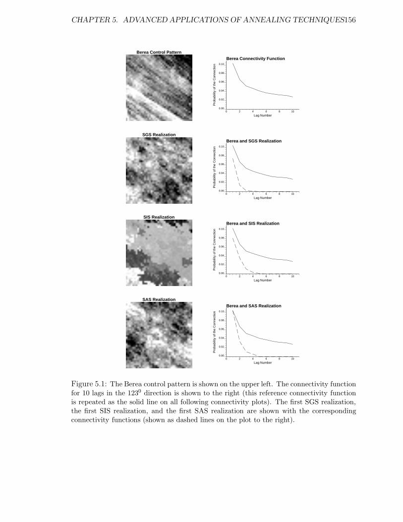
CHAPTER 5. ADVANCED APPLICATIONS OF ANNEALING TECHNIQUES156
Berea Control PatternBerea Connectivity Function
Lag Number
Pro
babi
lity
of th
e C
onne
ctio
n
0 2 4 6 8 100.00
0.02
0.04
0.06
0.08
0.10
SGS RealizationBerea and SGS Realization
Lag Number
Pro
babi
lity
of th
e C
onne
ctio
n
0 2 4 6 8 100.00
0.02
0.04
0.06
0.08
0.10
SIS RealizationBerea and SIS Realization
Lag Number
Pro
babi
lity
of th
e C
onne
ctio
n
0 2 4 6 8 100.00
0.02
0.04
0.06
0.08
0.10
SAS RealizationBerea and SAS Realization
Lag Number
Pro
babi
lity
of th
e C
onne
ctio
n
0 2 4 6 8 100.00
0.02
0.04
0.06
0.08
0.10
Figure 5.1: The Berea control pattern is shown on the upper left. The connectivity functionfor 10 lags in the 1230 direction is shown to the right (this reference connectivity functionis repeated as the solid line on all following connectivity plots). The first SGS realization,the first SIS realization, and the first SAS realization are shown with the correspondingconnectivity functions (shown as dashed lines on the plot to the right).

CHAPTER 5. ADVANCED APPLICATIONS OF ANNEALING TECHNIQUES157
Full SIS Realization
Connectivity: Berea and Full SIS Realization
Lag Number
Pro
babi
lity
of th
e C
onne
ctio
n
.0 2.0 4.0 6.0 8.0 10.0 .000
.020
.040
.060
.080
.100
Figure 5.2: A realization generated with full Sequential Indicator Simulation and the cor-responding connectivity function (dashed line). The reference Berea connectivity functionis shown as the solid line.
thresholds.
The SGS algorithm does not have the flexibility to consider multiple-point con-
nectivity measures, φ(h; N ; zc), as conditioning data; and the SIS algorithm is unable
to consider multiple-point connectivity measures, φ(h; N ; zc), for N > 2. However,
annealing could be formulated to consider these connectivity functions by adding a
component to the objective function:
Oc =10∑i=1
[φmodel(h; i; zc) − φrealization(h; i; zc)]2 (5.2)
where the 10 connectivity functions correspond to i = 1, . . . , 10. Note that i = 2
corresponds to a two-point connectivity measure. Thus, Oc calls for a combination
of 1,2,. . . ,10-variate information.
To illustrate the post-processing potential of annealing, the realizations generated
in Chapter 4 and shown on Figure 5.1, were taken as initial images for further an-
nealing processing. The temperature in the annealing schedule was set to zero since a

CHAPTER 5. ADVANCED APPLICATIONS OF ANNEALING TECHNIQUES158
high starting temperature would destroy the initial structure by accepting all pertur-
bations early in the annealing procedure. The Berea reference, the initial realizations
of Figure 5.1, the post-processed realizations and all corresponding connectivity func-
tions are shown on Figure 5.3. The post-processing yields both a visual improvement
and a noticeable improvement in the connectivity function.
Although the connectivity function is closer to the reference after post processing it
remains significantly lower for most N . The objective function in the annealing was to
match both the variogram and the connectivity function. Moreover, to minimize the
perturbation from the original images, the temperature in the annealing schedule was
set to zero; consequently, the image is frozen before reaching a global optimum (i.e.,
a perfect match to both the two-point statistics and the connectivity function). Were
the additional requirement to match the two-point statistics relaxed, the connectivity
function would be honored more closely. For example, Figure 5.4 shows the result of
post processing the first SGS realization by retaining only two lags of the variogram (a
unit distance in the vertical direction and a unit distance in the horizontal direction)
and all previous 10 connectivity values. The post-processed connectivity function,
shown by the short dashed line, is now well reproduced. Note the artifact checkerboard
aspect of the post-processed image arising from the fact that the unit lag h in the
connectivity function is three horizontal grid units and two vertical grid units rather
than being defined as a continuous line.
Figure 5.5 shows the connectivity function of all 100 SAS realizations generated in
Chapter 4 before and after post-processing. The better reproduction of the connectiv-
ity function and the visual improvement in the images are interesting features. A more
consequential measure is the impact on the output space of uncertainty. One hundred
additional flow simulations, using exactly the same flow scenario as documented in
Chapter 4, were performed using the post-processed images. Figure 5.6 shows the
output space of uncertainty before and after conditioning to the connectivity func-
tion. Table 5.1 shows the 95% probability interval before and after conditioning to
the connectivity function. Note the significant 30% reduction in the width of the 95%
probability intervals.
This reduction in the output uncertainty is the direct result of adding relevant

CHAPTER 5. ADVANCED APPLICATIONS OF ANNEALING TECHNIQUES159
Berea Control PatternBerea Connectivity Function
Lag Number
Pro
babi
lity
of th
e C
onne
ctio
n
0 2 4 6 8 100.00
0.02
0.04
0.06
0.08
0.10
SGS Realization SGS Post ProcessedConnectivity: Berea and SGS Realization
Lag Number
Pro
babi
lity
of th
e C
onne
ctio
n
0 2 4 6 8 100.00
0.02
0.04
0.06
0.08
0.10
SIS Realization SIS Post ProcessedConnectivity: Berea and SIS Realization
Lag Number
Pro
babi
lity
of th
e C
onne
ctio
n
0 2 4 6 8 100.00
0.02
0.04
0.06
0.08
0.10
SAS Realization SAS Post ProcessedConnectivity: Berea and SAS Realization
Lag Number
Pro
babi
lity
of th
e C
onne
ctio
n
0 2 4 6 8 100.00
0.02
0.04
0.06
0.08
0.10
Figure 5.3: The Berea control pattern is shown on the upper left. The connectivity func-tion for 10 lags in the 1230 direction is shown to the right (reproduced as the solid line onall following connectivity plots). The first SGS realization, the first SIS realization, andthe first SAS realization before and after post processing are shown with the correspond-ing connectivity functions. The long dashed line is the connectivity function before postprocessing and the short dashed line is after post processing.

CHAPTER 5. ADVANCED APPLICATIONS OF ANNEALING TECHNIQUES160
SGS Post Processed
Connectivity: Berea and SGS Realization
Lag Number
Pro
babi
lity
of th
e C
onne
ctio
n
0 2 4 6 8 100.00
0.02
0.04
0.06
0.08
0.10
Figure 5.4: The first SGS realization post-processed to match the Berea connectivity func-tion. The solid line corresponds to the reference Berea image, the long dashed line tothe initial SGS realization (shown on Figure 5.3), and the short dashed line to the imageshown to the left. Note the artifacts caused by relaxing the constraint to match two-pointstatistics.
Response Variable SAS 95% Probability Interval %Realizations q0.025 q0.975 width reduction
Time to reach 5% before 3.49 7.25 3.76after 3.64 6.41 2.77 -26%
Time to reach 95% before 24.78 46.75 21.97after 27.52 41.11 13.59 -38%
Time to recover 50% before 14.57 26.52 11.95after 15.35 23.88 8.53 -29%
Table 5.1: Summary of SAS output response results before and after conditioning to includethe connectivity function.

CHAPTER 5. ADVANCED APPLICATIONS OF ANNEALING TECHNIQUES161
Connectivity: SAS Realizations
Lag Number
Pro
babi
lity
of th
e C
onne
ctio
n
0 2 4 6 8 10
0.00
0.02
0.04
0.06
0.08
0.10
Connectivity: SAS Realizations After Post Processing
Lag Number
Pro
babi
lity
of th
e C
onne
ctio
n
0 2 4 6 8 10
0.00
0.02
0.04
0.06
0.08
0.10
Figure 5.5: The connectivity function for all SAS realizations before and after post pro-cessing.

CHAPTER 5. ADVANCED APPLICATIONS OF ANNEALING TECHNIQUES162
Fre
quen
cy
.0 2.0 4.0 6.0 8.0 10.0
.000
.040
.080
.120
Response One: unconditional SASmean 5.1005
std. dev. 1.0397coef. of var .2038
maximum 7.6889upper quartile 5.7904
median 5.1028lower quartile 4.1890
minimum 3.2988F
requ
ency
20.0 30.0 40.0 50.0 60.0
.0000
.0100
.0200
.0300
.0400
.0500
.0600
.0700
.0800Response Two: unconditional SAS
mean 34.5353std. dev. 5.7947
coef. of var .1678
maximum 48.7835upper quartile 38.7852
median 34.2986lower quartile 29.7469
minimum 24.6263
Fre
quen
cy
10.0 15.0 20.0 25.0 30.0
.000
.020
.040
.060
.080
Response Three: unconditional SASmean 19.6551
std. dev. 3.2340coef. of var .1645
maximum 27.9956upper quartile 21.9916
median 19.3641lower quartile 17.0208
minimum 14.3032
Fre
quen
cy
.0 2.0 4.0 6.0 8.0 10.0
.000
.040
.080
.120
Response One: post-processed SASmean 4.9223
std. dev. .7714coef. of var .1567
maximum 6.6964upper quartile 5.5296
median 4.8612lower quartile 4.2540
minimum 3.5347
Fre
quen
cy
20.0 30.0 40.0 50.0 60.0
.000
.040
.080
.120Response Two: post-processed SAS
mean 33.3572std. dev. 4.0088
coef. of var .1202
maximum 43.1688upper quartile 36.7992
median 32.6902lower quartile 30.2014
minimum 26.8260
Fre
quen
cy
10.0 15.0 20.0 25.0 30.0
.000
.020
.040
.060
.080
Response Three: post-processed SASmean 18.9260
std. dev. 2.2749coef. of var .1202
maximum 24.0021upper quartile 20.6730
median 18.5639lower quartile 17.1932
minimum 14.8614
Figure 5.6: The simulated output distributions generated by the annealing realizationsbefore and after conditioning by the connectivity function. The upper histograms are forthe time to achieve 5% water cut, the middle histograms are for the time to achieve a 95%water cut, and the lower histograms are for the time to recover 50% of the oil. The blackdot in the box plot below each histogram is the true value obtained from the referenceimage, the three vertical lines are the 0.025 quantile, the median (0.5 quantile), and the0.975 quantile of the output distribution.

CHAPTER 5. ADVANCED APPLICATIONS OF ANNEALING TECHNIQUES163
global conditioning statistics; it is not the result of a different random function model.
Once again, accounting for uncertainty in the model statistics used in the objective
function has been left for future research.
There are times when a single realization is all that is required. That single real-
ization may be used for predictive purposes with no attached measure of uncertainty,
in which case, uncertainty in the model statistics is not relevant. To ensure that this
lone realization yields results close to the center of the output distributions it would
be desirable to reproduce exactly the model statistics. The following section describes
how annealing could be used for this purpose.
5.1.2 Multivariate Spatial Transformation
Realizations generated by conventional simulation techniques typically show signif-
icant ergodic fluctuations, see Figure 4.9, Figure 4.18, and Appendix B. In certain
situations these ergodic fluctuations are desirable since they may be used to represent
(model) uncertainty in the input statistics due to sparse sampling. When the goal is
a close match to the RF model statistics it is desirable to remove these fluctuations.
Removing the departures from the model univariate distribution allows the output
uncertainty attributable to the multivariate distribution (beyond the univariate level)
to be assessed. A bivariate transformation procedure would be needed to assess the
output uncertainty attributable beyond the bivariate level. An interesting avenue of
research would be to assess independently each of the factors contributing to the out-
put uncertainty. These contributing factors would depend on the underlying random
function model; thus, availability of a multivariate transformation procedure would
provide a tool to understand better the impact of different RF models.
Another motivation for a multivariate transformation procedure arises from the
increasingly common practice of retaining a single simulated realization as an im-
proved “estimated” map. Indeed, stochastic simulation algorithms have proven to
be much more versatile than traditional interpolation algorithms in reproducing the
full spectrum of data spatial variability and in accounting for data of different types

CHAPTER 5. ADVANCED APPLICATIONS OF ANNEALING TECHNIQUES164
and sources, whether hard or soft [137]. A single realization does not allow an assess-
ment of uncertainty; however, it is quicker to generate and process through a complex
transfer function1. Given that only one realization is going to be used, it is desirable
that this realization identifies all the input spatial statistics. In other words, the
sole realization to be retained should be such that its response values are as near as
possible to the center of the output response distributions.
A unique analytical univariate transformation is possible with the rank-preserving
graphical transform procedure discussed in section 4.3 (see also [90], p. 478), i.e,
z = F−1(F (l)(z′)) (5.3)
where F−1(·) is the inverse of the model distribution, F (l)(·) is the distribution for the
simulation, z′ is a simulated value from F (l)(z), and z is the transformed value. This
transformation procedure was used in section 4.3 to evaluate the reduction in the space
of uncertainty due to removing ergodic fluctuations in the univariate distribution.
Consider the transformation of a bivariate distribution
F (l)(u,u + h; z, z′), ∀ h, z, z′ of interest
to some reference bivariate distribution
F (u,u + h; z, z′), ∀ h, z, z′ of interest
The general algorithm for such a bivariate transformation involving more than two
points at a time would require much more than the bivariate cdf F (u,u + h; z, z′).
Indeed, consider the problem of drawing a joint realization of N RV’s Z(u + hi), i =
1, . . . , N conditioned by the set of all bivariate cdf’s F (u + hi,u + hj ; z, z′), i, j =
1, . . . , N . The general algorithm would proceed as follows:
• draw a uniform [0, 1] random number y1. The first z-simulated value is as in
(5.3):
z(u + h1) = F−1(y1) = z1
1For example, in the petroleum industry it is common practice to history match the final numericalmodel of the reservoir before using it for predictive purposes. History matching consists of fine tuningthe rock/fluid properties so that a forward simulation of past production yields the actual measuredresponse. It may not be practical to perform history matching on more than one stochastic model.

CHAPTER 5. ADVANCED APPLICATIONS OF ANNEALING TECHNIQUES165
• draw a second uniform random number y2 independent of y1. The second z-
simulated value is:
z(u + h2) = F−1u+h2|u+h1
(y2|z1) = z2,
where Fu+h2|u+h1(z|z1) is the ccdf of Z(u+h2) given Z(u+h1) = z1. Everything
is fine as long as there are only two RV’s Z(u + h1) and Z(u + h2). A problem
arises already for the third variable, because Z(u+h3) must be related not only
to Z(u + h2) but also to Z(u + h1).
• draw a third independent random number y3. The third z-simulated value is:
z(u + h3) = F−1u+h3|u+h1,u+h2
(y3|z1, z2) = z3,
where F−1u+h3|u+h1,u+h2
(y3|z1, z2) is the ccdf of Z(u + h3) given Z(u + h1) =
z1 and Z(u + h2) = z2. This last ccdf actually calls for the trivariate cdf
F (u + h1,u + h2,u + h3; z, z′, z′′). That trivariate cdf ensures the consistency
between the corresponding three bivariate cdf’s.
Annealing provides an approximate solution that does not call for the multivariate
cdf by constructing an objective function that measures the difference between the
realization’s bivariate distribution and the model distribution:
O =N∑
i=1
[F (u,u + hi; z, z
′) − F (u,u + hi; z, z′)]2
(5.4)
where N is the number of point (lags) to be considered, F (u,u + hi; z, z′) is the
experimental bivariate distribution of the image being transformed, and
F (u,u + hi; z, z′) is the model bivariate distribution assumed internally consistent.
In addition to these N bivariate possibilities, the objective function may include
summaries of the full bivariate distribution, e.g., a covariance or variogram function,
∑h
[γ(h) − γ(h)]2 (5.5)
where γ(h) is the realization variogram, and γ(h) is the reference variogram for
selected separation vectors h.

CHAPTER 5. ADVANCED APPLICATIONS OF ANNEALING TECHNIQUES166
The annealing procedure to lower such objective functions, (5.4) plus (5.5), was
described in Chapter 3 and is possible with the sasim program documented in Ap-
pendix E.
As an example, consider the simulation of an 1/0 indicator variable representing
the presence or absence of shale. An anisotropic indicator semivariogram model is
available that fully characterizes the bivariate spatial distribution of that binary shale
indicator. An initial image2 is shown on the upper left of Figure 5.7. The model semi-
variogram in the two directions (aligned with the sides of the square image) is shown
by the solid lines on the semivariogram plot to the right of the initial image. The
bullets represent the experimental semivariogram values computed from that initial
image. The sasim program was used to transform this initial image into identifying
the model semivariogram. The initial image was transformed into the lower left cor-
ner image of Figure 5.7. The resulting experimental indicator semivariogram, shown
as the bullets on the plot at the right, is extremely close to the model. It took 11.4
CPU seconds on a DEC 5000 to perform the initial indicator simulation (one cutoff)
and 7.2 CPU seconds to perform the annealing post processing.
As another example, consider a non-conditional simulated realization of the Berea
permeability data. A specific sequential Gaussian simulation (SGS) realization in
the normal space, before back transformation to permeability, is shown at the upper
right of Figure 5.8. The semivariogram for four lags in the two principal directions of
continuity are shown as the bullets on the plot at the lower left. The corresponding
model is shown as the solid lines. Annealing has been applied to transform this
image so that the semivariogram model is more closely reproduced. The image and
corresponding semivariogram after post processing are shown to the right. The local
structure of the image was changed significantly since there were no local conditioning
data. It took 7.74 CPU seconds on a DEC 5000 for the original SGS simulation and
11.72 seconds for the annealing post-processing. Recall that it only took 8.69 seconds
to generate a realization with annealing starting from a random image. Depending on
the spatial features of the initial image it may be faster to generate a realization with
2That initial image could be derived from any technique. In the case of Figures 5.7 and 5.8,realizations that show large departures (due to a lack of ergodicity) from the input variogram modelwere selected for post-processing.

CHAPTER 5. ADVANCED APPLICATIONS OF ANNEALING TECHNIQUES167
Realization to be Transformed
Var
iogr
am
Distance
Indicator Semivariogram
.0 5.0 10.0 15.0 20.0
.000
.100
.200
.300
After Transformation
Var
iogr
am
Distance
Indicator Semivariogram
.0 5.0 10.0 15.0 20.0
.000
.100
.200
.300
Figure 5.7: An initial realization of a 1/0 indicator variable is shown in the upper left.Annealing is used to transform this image to identify the semivariogram model (shown asthe solid line on both semivariogram plots).

CHAPTER 5. ADVANCED APPLICATIONS OF ANNEALING TECHNIQUES168
SGS Realization (Normal Space) Post Processed (Normal Space)V
ario
gram
Distance
Semivariogram Before Transformation
.0 4.0 8.0 12.0
.00
.20
.40
.60
.80
1.00
1.20
Var
iogr
am
Distance
Semivariogram After Transformation
.0 4.0 8.0 12.0
.00
.20
.40
.60
.80
1.00
1.20
Figure 5.8: A SGS realization (in the normal space) is shown in the upper left corner.Below this realization is the corresponding variogram reproduction for four lags in the twoprincipal directions (123o and 33o). Applying annealing with the objective to honor thevariogram model (shown as the solid line) leads to the realization shown in the upper right.The variogram of this post processed image honors the variogram very closely.

CHAPTER 5. ADVANCED APPLICATIONS OF ANNEALING TECHNIQUES169
full simulated annealing starting from a random image rather than post-processing.
However, the main advantage of annealing over more conventional RF-based
stochastic simulation techniques is that the objective function can include more than
two-point statistics. The following section illustrates how a correlation coefficient with
a secondary variable could be used as a component in a global objective function.
5.1.3 Accounting for a Secondary Variable
In stochastic reservoir modeling there are usually very few direct (hard) measurements
of the attributes being mapped. Often, direct measurements are available only at well
locations and, typically, there are few wells within any one zone of the reservoir. Geo-
physical techniques provide additional measurements of sonic properties, available at
many locations, that may be correlated with the rock properties being mapped. The
quality of geophysical measurements has increased, through the use of high resolution
3-D seismic and inter-well measurements, and it now brings significant information
about the spatial distribution of rock properties such as porosity [60]. Any good sim-
ulation methodology must integrate all relevant information. Integrating geophysical
information is possible in an interpolation mode with cokriging approaches [43, 140]
or some type of trend model [100]; it is also possible to perform that integration with
annealing in a stochastic simulation mode.
The annealing algorithm described below to integrate seismic data may be gener-
alized to any situation where a secondary variable is available. For example, mapping
natural methane seepage per unit land area given sparse direct measurements and
near exhaustive satellite measurements [106].
An essential piece of information needed to account for a y-secondary variable is
a measure of correlation between the Z-primary and Y -secondary variables. When
the Z-Y correlation is very good then stochastic images of the primary z-variable will
look like the map of the secondary variable rescaled to the z-units; however, when
there is little correlation the map of the z-variable need not bear any resemblance
to the map of the y-variable. One aspect of the Z-Y correlation is reflected by the
scatterplot of collocated z-y measurements. Figure 5.9 shows an example calibration

CHAPTER 5. ADVANCED APPLICATIONS OF ANNEALING TECHNIQUES170
Z -
val
ues
Y - values
Calibration Scattergram
Y(l-1) Y(l)
Prior z-pdf for class [ Y(l-1),Y(l)]
Figure 5.9: Example calibration scatterplot and the prior z-probability pdf where thesecondary variable is y in the range (yl−1, yl].
scatterplot and the corresponding conditional distribution of z-values given a specific
range of y values. A number of such conditional distributions may be extracted from
the calibration scatterplot to allow for a reasonably complete characterization of the
Z-Y relationship [140].
In many cases, the z-y correlation may be further summarized by the linear cor-
relation coefficient:
ρ =Cov(Y, Z)
σZ · σY(5.6)
The correlation coefficient between measured y-secondary values and simulated z
values at the same location could be considered as a component in the objective
function of an annealing simulation, i.e.,
Oc = [ρcalibration − ρrealization]2 (5.7)
Recall that the key criterion for a quantity to enter the objective function is that it
must be locally updatable. The correlation coefficient meets this criterion. Consider
the following computational formula,
ρ =E{Z · Y } − E{Z} · E{Y }√
(E{Z · Z} − E{Z} · E{Z}) · (E{Y · Y } − E{Y } · E{Y })(5.8)
where the expected values are replaced by discrete summations over the N locations
in the area of interest, e.g., E{Z · Y } is evaluated by ( 1N
∑Ni=1 zi · yi).

CHAPTER 5. ADVANCED APPLICATIONS OF ANNEALING TECHNIQUES171
The correlation coefficient of the N simulated nodes, ρrealization, is locally updat-
able by updating each of the 5 summations, e.g., given a change from zoldi to znew
i the1N
∑Ni=1 zi · yi summation is updated as follows:
[1
N
N∑i=1
zi · yi
]new
=
[1
N
N∑i=1
zi · yi
]old
− 1
N
[(zold
i − znewi
)· yi
].
The other four summations are similarly updated. Moreover, if the annealing pertur-
bation mechanism is swapping then only 1N
∑Ni=1 zi ·yi need be updated. The measured
y-values never change and, in the case of swapping, the univariate distribution of the
z-values does not change.
An Example
A data set with 74 wells and a 3-D seismic survey were provided to the Stanford Center
for Reservoir Forecasting (SCRF) by Amoco Production Company in December 1990.
This data set, taken from a producing oil field in West Texas, was subjected to an
exhaustive geostatistical study [25]. One goal of the study was to generate realizations
of the 2-D vertically-averaged well porosity using both the well data and the 3-D
seismic energy data. This stochastic simulation exercise is repeated here with the
annealing-based approach.
The 74 well locations with gray-level coded porosity values are shown on the plan
map of Figure 5.10. The area enclosed by the solid border is 14000 feet by 15000
feet3. The inner area enclosed by the dashed line is a square 10400 feet by 10400 feet
area covered by 16900 CDP locations at which the sonic properties of the reservoir
have been measured. All future images of this reservoir are shown over the 10400 feet
by 10400 inner feet area covered by the seismic at an 80 by 80 foot resolution (130
by 130 blocks).
A histogram of the 74 porosity values is shown on the left of Figure 5.11. The
mean is 7.9 %, the coefficient of variation is a low 0.23, and there is no significant
skewness. The omnidirectional normal scores semivariogram of the porosity values
3The coordinates have been transformed to ensure confidentiality while preserving the spatialfeatures.

CHAPTER 5. ADVANCED APPLICATIONS OF ANNEALING TECHNIQUES172
12000-3000-2000
12000
Location Map of Well Data
4.0
4.8
5.6
6.4
7.2
8.0
8.8
9.6
10.4
11.2
12.0
Figure 5.10: A location map of the 74 well data with the porosity coded by the gray-levelof the location circles. The inner dashed line defines the area covered by the 3-D seismicsurvey.
computed from the 74 well data is shown on Figure 5.12. The horizontal dashed line
is at the unit variance of the standard normal distribution. The solid line on this
semivariogram plot is a model with a nugget effect of 20% and a single structure
spherical model with a range of 7500 feet. This semivariogram model is retained as
the sole measure of spatial continuity of porosity.
Figure 5.13 shows the gray-level coded seismic energy map. A histogram of the
16900 seismic data values is shown on the right of Figure 5.11. As shown on Fig-
ure 5.10, 19 of the 74 wells fall outside the area covered by the seismic; this leaves 55
pairs of z-porosity values and y-seismic values to establish the calibration scatterplot
shown on Figure 5.14. The linear correlation coefficent (ρ) is 0.535.
Stochastic models of the porosity should honor the sample histogram of porosity
(right of Figure 5.11), the spatial variability of porosity (variogram of Figure 5.12),
and the correlation with the seismic data. Conventional sequential Gaussian simu-
lation (SGS) would yield realizations like the two shown on Figure 5.15. Note that
the gray scale is identical to that used for the location map shown on Figure 5.10.

CHAPTER 5. ADVANCED APPLICATIONS OF ANNEALING TECHNIQUES173
Fre
quen
cy
Variable
0.0 4.0 8.0 12.0 16.0
0.000
0.040
0.080
0.120
Well Porosity Data Number of Data 74
mean 7.89std. dev. 1.78
coef. of var 0.23
maximum 11.38upper quartile 9.60
median 7.57lower quartile 6.49
minimum 3.87
Fre
quen
cy
Variable
0. 5000. 10000. 15000. 20000. 25000.
0.0000
0.0100
0.0200
0.0300
0.0400
0.0500
Seismic Energy Number of Data 16900
mean 9309.8std. dev. 5776.2
coef. of var 0.62
maximum 27700.0upper quartile 13200.0
median 8910.0lower quartile 4850.0
minimum 0.0
Figure 5.11: Histograms of 74 2-D vertically-averaged well porosity values and 16900seismic energy values.
Var
iogr
am
Distance
Porosity Normal Score Semivariogram
0. 2000. 4000. 6000. 8000. 10000.
0.00
0.40
0.80
1.20
Figure 5.12: The normal scores semivariogram based on 74 porosity values is shown by thebullets. The fitted model is shown by the solid line.
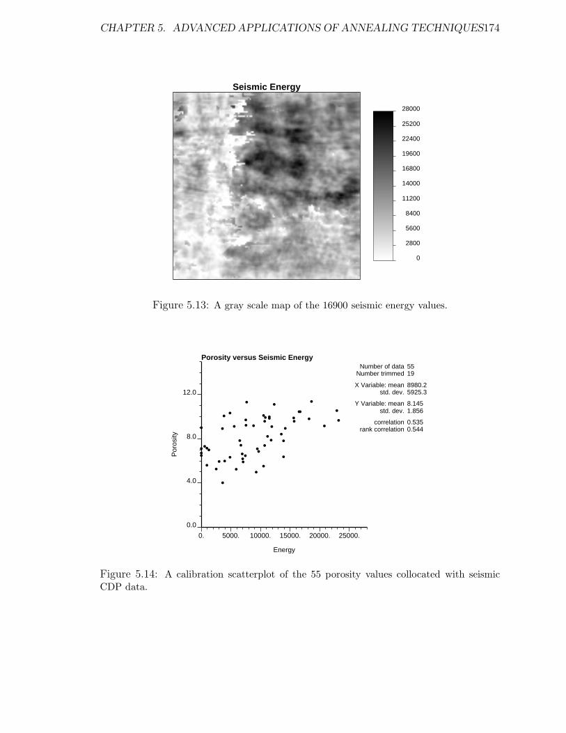
CHAPTER 5. ADVANCED APPLICATIONS OF ANNEALING TECHNIQUES174
Seismic Energy
0
2800
5600
8400
11200
14000
16800
19600
22400
25200
28000
Figure 5.13: A gray scale map of the 16900 seismic energy values.
Por
osity
Energy
Porosity versus Seismic Energy
0. 5000. 10000. 15000. 20000. 25000.
0.0
4.0
8.0
12.0
Number of data 55Number trimmed 19
X Variable: mean 8980.2std. dev. 5925.3
Y Variable: mean 8.145std. dev. 1.856
correlation 0.535rank correlation 0.544
Figure 5.14: A calibration scatterplot of the 55 porosity values collocated with seismicCDP data.

CHAPTER 5. ADVANCED APPLICATIONS OF ANNEALING TECHNIQUES175
First SGS Realization Second SGS Realization
Figure 5.15: Two sequential Gaussian realizations of the porosity.
These realizations are not built to honor the correlation with the calibration seis-
mic data. The correlation coefficient between the simulated porosity values and the
seismic values is 0.42 and 0.46 respectively for the first and second realization4.
Annealing could be used either to post-process the SGS realizations or to gener-
ate realizations with the sample histogram (Figure 5.11) and variogram model (Fig-
ure 5.12). The latter option was considered here: the sasim program was set up to
simulate directly the porosity with the objective function:
O = λ1
N∑i=1
[γmodel(hi) − γrealization(hi)]2 + λ2 [ρcalibration − ρrealization]2 (5.9)
The N = 18 separation vectors hi are defined by the most compact arrangement of 18
lags, see Figure 5.16. The ρcalibration = 0.535 is taken from the calibration scatterplot
shown on Figure 5.14.
Two realizations were generated with the two part objective function (5.9). Fig-
ure 5.17 shows how each component in the objective function changes as the sim-
ulation proceeds (the solid line is the deviation from the model variogram and the
4The correlation coefficient is high thanks to the many conditioning data used. With no condi-tioning data the correlation coefficient would be zero.
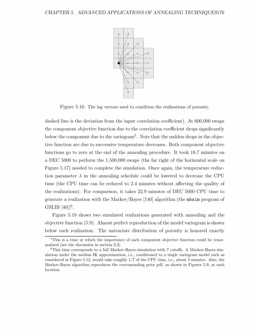
CHAPTER 5. ADVANCED APPLICATIONS OF ANNEALING TECHNIQUES176
Figure 5.16: The lag vectors used to condition the realizations of porosity.
dashed line is the deviation from the input correlation coefficient). At 600,000 swaps
the component objective function due to the correlation coefficient drops significantly
below the component due to the variogram5. Note that the sudden drops in the objec-
tive function are due to successive temperature decreases. Both component objective
functions go to zero at the end of the annealing procedure. It took 18.7 minutes on
a DEC 5000 to perform the 1,500,000 swaps (the far right of the horizontal scale on
Figure 5.17) needed to complete the simulation. Once again, the temperature reduc-
tion parameter λ in the annealing schedule could be lowered to decrease the CPU
time (the CPU time can be reduced to 2.4 minutes without affecting the quality of
the realizations). For comparison, it takes 22.9 minutes of DEC 5000 CPU time to
generate a realization with the Markov/Bayes [140] algorithm (the mbsim program of
GSLIB [40])6.
Figure 5.18 shows two simulated realizations generated with annealing and the
objective function (5.9). Almost perfect reproduction of the model variogram is shown
below each realization. The univariate distribution of porosity is honored exactly
5This is a time at which the importance of each component objective function could be renor-malized (see the discussion in section 3.2)
6This time corresponds to a full Markov-Bayes simulation with 7 cutoffs. A Markov-Bayes sim-ulation under the median IK approximation, i.e., conditioned to a single variogram model such asconsidered in Figure 5.12, would take roughly 1/7 of the CPU time, i.e., about 3 minutes. Also, theMarkov-Bayes algorithm reproduces the corresponding prior pdf, as shown in Figures 5.9, at eachlocation.

CHAPTER 5. ADVANCED APPLICATIONS OF ANNEALING TECHNIQUES177
Objective Function versus Time
Number of swaps (1000’s)
Obj
ectiv
e F
unct
ion
0 400 800 1200
0.0
0.2
0.4
0.6
0.8
1.0
Figure 5.17: The two component objective functions are plotted versus the number ofswaps. The solid line is due to the deviation from the model variogram and the dashed lineis due to the deviation of the correlation coefficient from the observed value of 0.535.
at the beginning by assigning the original nodal values by random drawing from
that reference distribution. The swapping perturbation mechanism considered in this
case does not alter the initial histogram. In both cases, the correlation coefficient
(0.535) between the simulated porosity values and seismic data has been exactly
reproduced. Figure 5.19 shows a scatterplot of the simulated porsity values from the
first realization and the seismic data, to be compared with the sample scatterplot of
Figure 5.14.
These annealing realizations appear as plausible images of the 2-D vertically av-
eraged porosity; the input control statistics are almost perfectly reproduced. These
realizations indicate a continuous zone of high porosity in the center of the map with
low porosity zones in the lower left and lower right corners. The SGS realizations
(Figure 5.15), which did not consider the seismic data, do not reveal these features
as clearly.
This example illustrates how annealing can be used to integrate geophysical in-
formation. The next section presents more examples of how annealing, with multiple

CHAPTER 5. ADVANCED APPLICATIONS OF ANNEALING TECHNIQUES178
First Annealing Realization Second Annealing Realization
Sem
ivar
iogr
am
Distance
Semivariogram: Realization One
0. 1000. 2000. 3000. 4000. 5000. 6000.
.00
1.00
2.00
3.00
Sem
ivar
iogr
am
Distance
Semivariogram: Realization Two
0. 1000. 2000. 3000. 4000. 5000. 6000.
.00
1.00
2.00
3.00
Figure 5.18: Two realizations generated with annealing to match specified lags of thevariogram (see Figure 5.16) and the correlation with the seismic data. The omnidirectionalsemivariogram of each image is shown below the corresponding realization.

CHAPTER 5. ADVANCED APPLICATIONS OF ANNEALING TECHNIQUES179
Por
osity
Seismic
Porosity versus Seismic Energy
0. 5000. 10000. 15000. 20000. 25000.
0.0
4.0
8.0
12.0
Number of data 16900
X Variable: mean 9309.763std. dev. 5776.214
Y Variable: mean 7.898std. dev. 1.829
correlation 0.535rank correlation 0.540
Figure 5.19: A scatterplot of the simulated porosity values (first realization) and the seismicdata. Note that the correlation coefficient is exactly the reference value of 0.535.
component objective functions, can be used to integrate complex geological struc-
tures.
5.2 Geological Structures
The objective function can be formulated to account for multiple-point statistics
(section 3.3) so that complex geological structures could be more realistically charac-
terized, and reproduced. Consequently, the resulting distributions of output response
variables should be more accurate.
An example is presented in the next section 5.2.1 where a reference image (ob-
tained by scanning a photograph) is analyzed through traditional two-point statistics
and then with multiple-point statistics. Simulated realizations are shown to demon-
strate visually the improvement brought by considering annealing to reproduce these
multiple-point statistics.
The visual appearance of simulated realizations is important; the human eye can

CHAPTER 5. ADVANCED APPLICATIONS OF ANNEALING TECHNIQUES180
be very sensitive to the features shared by a simulated realization and a reference im-
age. However, goodness criteria must be based on the output distributions generated
after processing these realizations through a transfer function. A case study based on
reference data taken from a cross-stratified sands and silty sands distributary-mouth
bar environment is developed in section 5.2.2. The improvement brought by annealing
and multiple-point statistics is quantified in the output space of uncertainty.
5.2.1 An Example Application: eolian Sandstone
The eolian sandstone environment illustrated by the image shown at the top of Fig-
ure 5.20 poses severe problems for traditional stochastic imaging methods. This image
represents one side of a thin rectangular parallelepiped (1 cm by 10 cm by 20 cm) cut
from an eolian sandstone. The scanned image shown at the top of Figure 5.20 has
328 by 171 square pixels each with a continuous gray level value between 0 (white)
and 1 (black). The white areas represent clean well sorted sandstone with high per-
meability and the dark areas represent finer grained sandstone with low permeability.
For computational ease this original image was upscaled to the image shown at the
bottom of Figure 5.20. The upscaled image has 164 by 85 square integer-coded pixels
with an integer gray level code ranging from 1 (white) to 8 (black).
The normal scores variogram of the eolian sandstone is shown on Figure 5.21.
Note the significant anisotropic periodicity and the 6:1 anisotropy. All distances are
relative to the discretization units of the upscaled image with the image being 164
distance units by 85 distance units. The following model was considered, with (h1, h2)
being the coordinates in the two directions corresponding to the sides of the image:
γY (h) = 0.45 · Sph
√
h21
2.02+
h22
5.02
+ 0.22 · Sph
√
h21
0.52+
h22
5.02
+ 0.45 · Exp
√
h21
0.000012+
h22
40.02
+ 0.27 · DH17.0,0.298
(√h2
1
)

CHAPTER 5. ADVANCED APPLICATIONS OF ANNEALING TECHNIQUES181
Original Eolian Sandstone
Upscaled Eolian Sandstone
Figure 5.20: The original scanned image of the eolian sandstone with the upscaled reference.

CHAPTER 5. ADVANCED APPLICATIONS OF ANNEALING TECHNIQUES182
Var
iogr
am
Distance
Normal Scores Semivariogram
.0 10.0 20.0 30.0 40.0 50.0
.00
.20
.40
.60
.80
1.00
1.20
Figure 5.21: Normal scores variogram of the eolian sandstone in the two principal direc-tions.
(5.10)
Sph(h) is the unit range spherical variogram model defined as:
Sph(h) =
[1.5h − 0.5h3] , if h ≤ 1
1, if h ≥ 1
Exp(h) is the exponential variogram function with effective range 3 defined as:
Exp(h) = [1 − exp(−h)]
and DHd,a(h) is a dampened hole effect cosine model defined as:
DHd,a(h) = 1.0 − exp
(−h · ad
)· cos (h · a)
There are four components in the semivariogram model (5.10):
1. a short scale anisotropic spherical structure that explains 40% of the total vari-
ability (the longer range is in the horizontal h2 direction and the shorter range
is in the vertical h1 direction).

CHAPTER 5. ADVANCED APPLICATIONS OF ANNEALING TECHNIQUES183
2. a second short scale anisotropic spherical structure (with a more pronounced
anisotropy along the same horizontal and vertical directions) that explains an
additional 20% of the variability,
3. a third anisotropic long range exponential structure (the range parameter is
40.0, thus, the effective range is 120.0 in the horizontal direction and 0.0 in the
vertical direction ) that explains 40% of the variability, and
4. finally, a dampened hole effect model in the vertical direction to account for the
periodicity.
Two realizations based on a Gaussian simulation algorithm (program sgsim in
GSLIB [40]) were generated and are shown on Figure 5.22. As expected the real-
izations fail to show the curvilinear well connected structures of the reference image.
The indicator variograms for the quintiles of the univariate distribution of the
eolian sandstone have been modeled with the same nested structures as the normal
scores variogram. Two realizations based on a indicator simulation algorithm (pro-
gram sisim in GSLIB [40]) were generated and are shown on Figure 5.23. Once again,
the realizations do not show the curvilinear structures or the connected features of
the reference image.
Even limited to two-point statistics the image is better characterized with full
two-point histograms which contain all of the direct and cross indicator covariances.
This possibility was considered by using the annealing program sasim (described in
Chapter 3 and documented in Appendix E). The two-point histogram for 10 lags
in four directions (offsets [1,0], [0,1], [2,1], [2,-1]) were imposed. The post-processed
realizations are shown on Figure 5.24.
Two-points statistics do a poor job of characterizing the curvilinear highly con-
nected features of this image. Boolean or marked-point processes would also be inap-
propriate due to the complex interaction between the curvilinear shapes. Simulation
procedures using multiple-point statistics would be needed to capture the curvilinear
features of this image.

CHAPTER 5. ADVANCED APPLICATIONS OF ANNEALING TECHNIQUES184
Gaussian Simulation Two
Gaussian Simulation One
Figure 5.22: Two Gaussian-based simulated realizations of the eolian sandstone.

CHAPTER 5. ADVANCED APPLICATIONS OF ANNEALING TECHNIQUES185
Indicator Simulation Two
Indicator Simulation One
Figure 5.23: Two indicator-based simulated realizations of the eolian sandstone.

CHAPTER 5. ADVANCED APPLICATIONS OF ANNEALING TECHNIQUES186
Indicator Simulation Two: processed
Indicator Simulation One: processed
Figure 5.24: Two post processed indicator-based simulated realizations of the eolian sand-stone.

CHAPTER 5. ADVANCED APPLICATIONS OF ANNEALING TECHNIQUES187
Figure 5.25: A scanned photograph of core from a distributary-mouth bar sequence [118].The darker gray levels correspond to a greater proportion of clayey/silty material. Theactual image is approximately 6 inches by 3 inches.
5.2.2 Impact on Output Response Uncertainty
In the following case-study an exhaustively sampled reference image will be repro-
duced through stochastic simulations based on RF models differing by the statistics
which constrain them. It will be shown that different models though sharing the
same covariance function C(h) and the same univariate distribution lead to real-
izations with different spatial characteristics [87] and, more importantly, result in a
different assessment of the response uncertainty.
Figure 5.25 is an image of cross-stratified sands and silty sands from a distributary-
mouth bar taken from page 151 of Sandstone Depositional Environments [118]. Fig-
ure 5.25 is approximately at 1:1 scale (6 inch by 3 inch). The grayness of the image
has been arbitrarily scaled through a monotonic function into permeability values to
yield the discrete histogram of Figure 5.26.
The reference image of Figure 5.25 is discretized into 225 x 125 square pixels. For
the rest of this study, the data and image of Figure 5.25 will be considered as the

CHAPTER 5. ADVANCED APPLICATIONS OF ANNEALING TECHNIQUES188
Fre
quen
cy
Permeability, md
0. 20. 40. 60. 80. 100.
0.000
0.050
0.100
0.150
0.200
0.250Reference Permeability Distribution
Number of Data 28125mean 10.0
std. dev. 13.96coef. of var 1.39
maximum 323.8upper quartile 13.4
median 5.23lower quartile 1.05
minimum 0.0
Figure 5.26: Distribution of the reference permeability values (md).
“true” reference to be reproduced.
The reference image will be simulated using various RF models conditioned by
various global statistics such as the covariance. However, no local conditioning will
be considered, that is, no samples will be retained from the reference image.
Gaussian Model
The reference permeability values are first transformed into a standard normal distri-
bution through a normal scores transform. Then a multivariate Gaussian RF model
is adopted for these normal scores transforms. This Gaussian RF model is fully char-
acterized by the variogram of the normal scores transforms shown in Figure 5.27. The
experimental (exhaustive) variogram of the reference normal scores has been modeled
by the nested sum of three structures, a nugget effect of 0.20, a short scale exponen-
tial structure contributing 0.55 of the total unit variance and a larger scale spherical
structure contributing 0.25; both structures are anisotropic:

CHAPTER 5. ADVANCED APPLICATIONS OF ANNEALING TECHNIQUES189
Var
iogr
am
Distance
Normal Scores Variogram
.0 10.0 20.0 30.0 40.0 50.0
.00
.20
.40
.60
.80
1.00
Figure 5.27: Semivariograms of the normal score transforms of the reference data of Fig-ure 5.25 along the vertical (upper set of curves) and horizontal directions (lower set). Thesolid lines are the model fits.
γ(hx, hy) = 0.20 + 0.55Exp
√√√√(hx
10
)2
+
(hy
1.6
)2 (5.11)
+ 0.25Sph
√√√√( hx
180
)2
+
(hy
15
)2
with Exp(h) and Sph(h) as defined in (5.10). hx and hy are the horizontal and vertical
coordinates.
The sequential Gaussian simulation algorithm and GSLIB program sgsim [40] was
used to generate 100 simulated realizations of the permeability normal scores field,
conditioned to the previous variogram model. These normal scores realizations are
then back-transformed using the reference permeability distribution of Figure 5.26.
Consequently, all back-transformed realizations exactly reproduce the original his-
togram of Figure 5.26. The first two generated permeability realizations are shown
on Figure 5.28.

CHAPTER 5. ADVANCED APPLICATIONS OF ANNEALING TECHNIQUES190
Figure 5.28: Two realizations from the Gaussian model.

CHAPTER 5. ADVANCED APPLICATIONS OF ANNEALING TECHNIQUES191
Figure 5.28 is to be compared to Figure 5.25. Note the characteristic “salt-and-
pepper” appearance of the Gaussian images, a consequence of the maximum entropy
character of the underlying RF model (see Appendix C).
The slight 10o dip of the structures seen on Figure 5.25 is not reproduced on
Figure 5.28 for the simple reason that only the vertical to horizontal anisotropy was
modeled.
Median IK Model
The median IK model represents an alternative to the Gaussian RF model in that it
is also fully characterized by a single covariance function, yet its multivariate distri-
bution is non-Gaussian.
The median IK or mosaic model is a bivariate mixture of two binormal distribu-
tions with common univariate Gaussian distribution. The first binormal distribution
has a correlation coefficient of 1 (i.e., all values are equal) and the second a correla-
tion coefficient of 0 (i.e., all values are independent). A mixture of these two bivariate
Gaussian distributions with proportion p(h) yields the following bivariate cumulative
distribution function [101].
Prob{Y (u) ≤ y, Y (u + h) ≤ y′} (5.12)
= p(h)G(min(y, y′)) + [1 − p(h)]G(y)G(y′)
where Y (u) represents the stationary RF model with standard normal cumulative
distribution function (cdf): G(y) = Prob{Y (u) ≤ y}, ∀u.
The previous bivariate distribution (5.12) corresponds to a RF model Y (u) such
that Y (u) and Y (u + h) are equal with probability p(h) and independent with the
complement probability [1 − p(h)]. It can be shown that the correlogram and all
indicator correlograms of the RF Y (u) are equal to p(h):
CY (h)
CY (0)= p(h) (5.13)
with: CY (h) = Cov{Y (u), Y (u + h)}, and:
CI(h; y, y′)CI(0; y, y′)
= p(h) ∀y, y′ (5.14)

CHAPTER 5. ADVANCED APPLICATIONS OF ANNEALING TECHNIQUES192
with: CI(h; y, y′) = Cov{I(u; y), I(u + h; y′)}and: I(u; y) = 1 if Y (u) ≤ y; = 0 if not.
One hundred realizations of the median IK model were generated using the pro-
gram sisim of GSLIB [40]; the two first generated realizations are given on Fig-
ure 5.29. Once again, all realizations share, by construction, the original histogram
of Figure 5.26.
Figure 5.29 is to be compared to Figure 5.25 for the reference and to Figure 5.28
for the Gaussian model. Remember that all images share the same histogram, i.e.,
the same proportion of high/median/low permeability values, and the same variogram
model (5.11) for normal score transforms. Hence any difference is due to the implicit
RF model beyond histogram and covariance.
The visual difference between the Gaussian and median IK realizations is quite
striking, with the median IK realizations presenting clearer spatial structures.
Multiple Indicator Model
One should question retaining the covariance as the sole spatial characteristic of an
image (or equivalently the covariance of its normal scores transform). By extracting
more structural information from the reference or sampled image, one should be able
to reproduce more of the spatial features of the reference image. Experience has
shown that whenever sampling allows inference of the attribute covariance C(h) it
also allows inference of its indicator covariances, at least for threshold values z, z′ that
are not too extreme. Thus, consider simulation of the reference image of Figure 5.25
by retaining some of its indicator covariances/variograms.
Seven threshold values zk = 0.1, 2.5, 5.0, 7.5, 10.0, 15.0, and 30.0 md, k = 1, . . . , 7
were retained which correspond to the 0.20, 0.35, 0.48, 0.60, 0.67, 0.80, and 0.92
quantiles of the exhaustive reference distribution of Figure 5.26. The indicator RF is
then defined for each threshold zk as:
I(u; zk) = 1, if permeability Z(u) ≤ zk; = 0 if not.
The corresponding exhaustive variograms in the vertical and horizontal directions,
together with their fitted models are given in Figure 5.30. All models are standardized
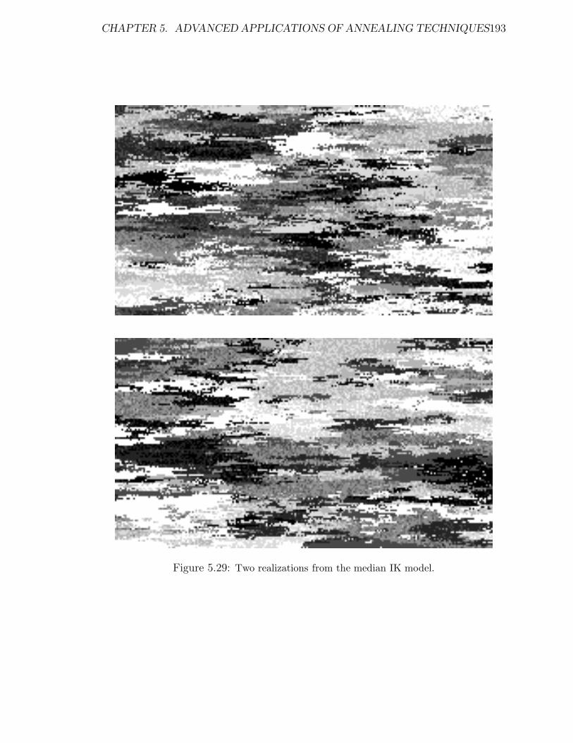
CHAPTER 5. ADVANCED APPLICATIONS OF ANNEALING TECHNIQUES193
Figure 5.29: Two realizations from the median IK model.

CHAPTER 5. ADVANCED APPLICATIONS OF ANNEALING TECHNIQUES194
Threshold Exponential Structure Spherical Structurek quantile C0() C1() a1() b1() C2() a2() b2()1 0.20 0.17 0.50 18.0 7.8 0.33 100.0 10.02 0.35 0.11 0.54 47.7 14.4 0.35 150.0 15.03 0.48 0.13 0.58 90.0 18.0 0.29 170.0 17.04 0.60 0.13 0.61 90.0 14.5 0.26 160.0 16.05 0.67 0.12 0.68 108.0 17.4 0.20 91.0 12.86 0.80 0.12 0.68 108.0 15.2 0.20 85.0 12.07 0.92 0.22 0.69 144.0 21.5 0.09 66.0 11.2
Table 5.2: Reference indicator variograms parameters. The ranges a1(), b1(), a2(), b2() areexpressed in pixel units. The relative sill values C0(), C1(), C2() are dimensionless.
to a unit sill with the following combination of nugget effect, short range exponential
structure, and longer range spherical structure:
γI(h; zk) = Co(zk) (5.15)
+ C1(zk)Exp
√√√√( hx
a1(zk)
)2
+
(hy
b1(zk)
)2
+ C2(zk)Sph
√√√√( hx
a2(zk)
)2
+
(hy
b2(zk)
)2
with Exp() and Sph() defined as in (5.11).
Table 5.2 gives the corresponding model parameters. Some remarks:
• The relative nugget effect is larger for the two extreme threshold values (first
and last); however, this “destructuring” of extreme values is not symmetric,
as would be implied by a Gaussian model [83]: the nugget effect for the 0.20
quantile is different from that for the 0.80 quantile (0.17 �= 0.12).
• The relative contribution, ranges and anisotropy ratios, of the medium range
exponential structure increases consistently from the first to last threshold.
• The relative contribution of the larger range spherical structure decreases con-
sistently from the first through the last threshold.

CHAPTER 5. ADVANCED APPLICATIONS OF ANNEALING TECHNIQUES195
Var
iogr
am
Distance
First Cutoff
.0 10.0 20.0 30.0 40.0 50.0
.0000
.0100
.0200
.0300
.0400
.0500
.0600
.0700
Var
iogr
am
Distance
Second Cutoff
.0 10.0 20.0 30.0 40.0 50.0
.000
.040
.080
.120
Var
iogr
am
Distance
Third Cutoff
.0 10.0 20.0 30.0 40.0 50.0
.000
.040
.080
.120
.160
Var
iogr
am
Distance
Fourth Cutoff
.0 10.0 20.0 30.0 40.0 50.0
.000
.050
.100
.150
.200
Var
iogr
am
Distance
Fifth Cutoff
.0 10.0 20.0 30.0 40.0 50.0
.000
.050
.100
.150
.200
.250
Var
iogr
am
Distance
Sixth Cutoff
.0 10.0 20.0 30.0 40.0 50.0
.000
.050
.100
.150
.200
.250
Var
iogr
am
Distance
Seventh Cutoff
.0 10.0 20.0 30.0 40.0 50.0
.000
.040
.080
.120
.160
Figure 5.30: Reference indicator variograms and their fitted models.

CHAPTER 5. ADVANCED APPLICATIONS OF ANNEALING TECHNIQUES196
• Therefore, high and low permeability values are less correlated than the medium
values, with low values being better correlated than high values. These remarks
are somewhat corroborated by visual inspection of Figure 5.25.
One hundred realizations of the multiple indicator model were generated using
the program sisim of GSLIB [40]; the first two realizations are given on Figure 5.31.
Figure 5.31 is to be compared to Figures 5.25, 5.28, and 5.29 respectively. Re-
member that all images share the exact same histogram of permeability values, that
of Figure 5.26.
The realizations created with multiple indicator simulation are seen to reproduce
more of the reference spatial features. Another alternative is to use annealing with
multiple-point spatial statistics to obtain a better reproduction.
Annealing
By extracting more structural information from the reference image, one should be
able to reproduce more of the spatial features of the reference image. However,
extracting too much information would lead to too close reproduction of the reference
image; this is not the goal. The goal is to extract the salient or transportable features
that, in practice, could be used for mapping a sparsely sampled reservoir.
In this case the two-point histogram for 33 lags (see Figure 5.32) and four different
five-point indicator covariances aligned in the horizontal direction were retained.
One hundred realizations of the annealing model were generated using the program
sasimi documented in Chapter 3 and Appendix E; the first two realizations are given
on Figure 5.33.
Figure 5.33 is to be compared to Figures 5.25, 5.28, 5.29, and 5.31 respectively.
Note that the annealing realizations share more spatial features with the reference
image due to the additional global statistics that were retained for the simulation.
Flow Modeling
The output uncertainty given by each of the four RF models is quantified by pro-
cessing all 401 images (the reference image and 100 realizations from each of the four

CHAPTER 5. ADVANCED APPLICATIONS OF ANNEALING TECHNIQUES197
Figure 5.31: Two realizations from the multiple indicator model.

CHAPTER 5. ADVANCED APPLICATIONS OF ANNEALING TECHNIQUES198
Figure 5.32: Lags for two-point histogram control.
RF models) through a flow-related transfer function. The 2-D images were taken to
represent vertical cross sections between an injecting and a producing well.
The constant porosity grid blocks are initially saturated with oil and then sub-
jected to a water flooding with no-flow boundary conditions on the upper and lower
boundaries of the cross section. The Eclipse flow simulator [48] has been used for the
flow simulations. Both wells operate at constant bottom hole pressure, straight line
relative permeabilities were used, and both the oil and water have a unit mobility
ratio.
The following two flow response variables were isolated to characterize the flow
characteristics of each image:
• The effective permeability of the image. This parameter is computed once the
oil is completely swept from the image and the water flow rate has stabilized.
This response variable provides an overall steady state flow characteristic of the
image.
• The time at which the water cut reaches 90%. This response is a measure of
sweepage and late flow characteristics of the image.

CHAPTER 5. ADVANCED APPLICATIONS OF ANNEALING TECHNIQUES199
Figure 5.33: Two realizations from the annealing model.

CHAPTER 5. ADVANCED APPLICATIONS OF ANNEALING TECHNIQUES200
Case Time to reach 90% Effective Permeabilityq0.025 q0.5 q0.975 q0.025 q0.5 q0.975
Reference 8.33 3.70Gaussian 7.84 11.36 16.45 1.39 2.04 3.11Median IK 7.24 11.10 16.46 1.26 2.21 4.31Full Indicator 5.83 13.03 33.65 0.83 2.13 5.79Annealing 4.69 10.37 18.60 0.91 2.36 7.24
Table 5.3: Summary of output response values. The reference values of 8.33 md and 3.70time units are followed by the median q0.05 and the 95% probability interval (q0.025 andq0.975).
The flow simulation exercise described above was also carried out using the refer-
ence spatial distribution (Figure 5.25). The reference effective permeability was 8.33
md and the time to achieve a 90% water cut was 3.70 time units.
Figure 5.34 shows the histograms of effective permeability obtained from the four
RF models being considered. Figure 5.35 shows the histograms of the time to reach
90% water cut obtained from the four RF models. The effective permeability and the
time to achieve 90% water cut have a correlation of about -0.75 in all cases.
Table 5.3 gives the median (q0.5) and the 95% probability bounds (q0.025 and q0.975)
of the flow response variables for the four sets of simulations.
Observations
• The actual reference time value (3.70 time units) is not within the range of
the 100 Gaussian model-derived response values and barely within the ranges
of the median IK and indicator model-derived distributions. The reference
effective permeability (8.33 md) is only barely in the range of the Gaussian
model derived-distribution and fits only slightly better in the ranges of the
median IK and indicator model-derived distributions.
• Although all 400 realizations of the permeability field reproduce exactly the ref-
erence univariate distribution (Figure 5.25) they all yield distributions whose
centers (mean or median) deviate considerably from the reference value. The

CHAPTER 5. ADVANCED APPLICATIONS OF ANNEALING TECHNIQUES201
Fre
quen
cy
.0 10.0 20.0 30.0 40.0
.000
.100
.200
.300
.400
Gaussian Model: Effective Permeabilitymean 11.77
std. dev. 2.14coef. of var 0.182
maximum 18.16upper quartile 13.15
median 11.36lower quartile 10.21
minimum 7.23
Fre
quen
cy
.0 10.0 20.0 30.0 40.0
.000
.100
.200
.300
.400
Median IK Model: Effective Permeabilitymean 11.42
std. dev. 2.36coef. of var 0.21
maximum 18.84upper quartile 12.69
median 11.10lower quartile 9.67
minimum 6.33
Fre
quen
cy
.0 10.0 20.0 30.0 40.0
.000
.050
.100
.150
.200Indicator Model: Effective Permeability
mean 14.04std. dev. 6.12
coef. of var 0.44
maximum 35.03upper quartile 17.30
median 13.03lower quartile 9.05
minimum 5.03
Fre
quen
cy
.0 10.0 20.0 30.0 40.0
.000
.050
.100
.150
.200
Annealing Model: Effective Permeabilitymean 11.14
std. dev. 3.86coef. of var 0.35
maximum 19.78upper quartile 14.86
median 10.37lower quartile 8.10
minimum 3.73
Figure 5.34: Distribution of effective permeabilities obtained from the Gaussian, medianIK, indicator, and annealing RF models. The dot location gives the reference image value(8.33 md).

CHAPTER 5. ADVANCED APPLICATIONS OF ANNEALING TECHNIQUES202
Fre
quen
cy
.0 2.0 4.0 6.0 8.0
.000
.100
.200
.300
.400 Gaussian Model: Late Breakthroughmean 2.11
std. dev. 0.45coef. of var 0.22
maximum 3.48upper quartile 2.38
median 2.04lower quartile 1.77
minimum 1.18
Fre
quen
cy
.0 2.0 4.0 6.0 8.0
.000
.100
.200
.300
Median IK Model: Late Breakthroughmean 2.34
std. dev. 0.78coef. of var 0.33
maximum 6.81upper quartile 2.82
median 2.21lower quartile 1.83
minimum 1.14
Fre
quen
cy
.0 2.0 4.0 6.0 8.0
.000
.050
.100
.150
.200
Indicator Model: Late Breakthroughmean 2.41
std. dev. 1.30coef. of var 0.54
maximum 7.15upper quartile 3.12
median 2.14lower quartile 1.43
minimum 0.71
Fre
quen
cy
.0 2.0 4.0 6.0 8.0
.000
.050
.100
.150
.200
Annealing Model: Late Breakthroughmean 2.80
std. dev. 1.66coef. of var 0.59
maximum 8.60upper quartile 3.64
median 2.36lower quartile 1.45
minimum 0.78
Figure 5.35: Distribution of late breakthrough times obtained from the Gaussian, medianIK, indicator, and annealing RF models. The dot location gives the reference image value(3.70 time units).
CHAPTER 5. ADVANCED APPLICATIONS OF ANNEALING TECHNIQUES203
Gaussian model is the most inaccurate in the sense that it generates distribu-
tions of response values that do not even contain the true values. The annealing
model is centered closest to the reference values. This is expected since it re-
produces the most reference statistics.
• Note that the distributions of response values need not be Gaussian, nor even
symmetric: see the indicator model-derived histograms of Figures 5.34 and 5.35.
• The multiple indicator RF model is imprecise, in the sense that it yields the
largest variance for the posterior response distribution; but that imprecision
allows accuracy, in the sense that these distributions do include the actual
response values.
• A possible reason for the actual effective permeability (8.33md) to be so low
may be the cross-bedding of the low (white) permeability streaks visible on
Figure 5.25 and their concentration next to the left vertical well. Such infor-
mation is not accounted for in any of the three RF models. Were the 10o dip
of the direction of maximum continuity modeled and the continuity of the low
indicator RV’s increased (e.g., by setting the relative nugget effect C0(1) to zero
in Table 2), the multiple indicator RF model would likely have yielded better
results, i.e., response distributions better centered on the actual values.
• Purposely not to confuse the discussion on entropy, the stochastic simulations
were made non-conditional to local data, as obtained from the producer and
injector. In practice, no matter the RF model chosen, the realizations will be
made to honor local data whether originating from well logs or seismic data
(impedance or velocity); consequently, the realizations would be less different
one from another and also more accurate, i.e., closer to the actual image; con-
sequently, the posterior response distributions would be both more precise and
more accurate.
There is much more actual information to be collected from data than a mere
covariance of normal score transforms. In which case, the output distributions can
be estimated more accurately and precisely.

CHAPTER 5. ADVANCED APPLICATIONS OF ANNEALING TECHNIQUES204
.
5.3 Well Tests
An important reservoir parameter measured by a pressure transient well test is the
effective absolute permeability near the well bore. This effective permeability does
not directly inform the block permeabilities near the well bore; however, it does
constrain a complex non-linear average of the small scale block permeabilities. Many
flow processes are directly influenced by this effective permeability. For example,
the average flow rate for a fixed pressure gradient or the reservoir pressure behavior
under constant flow rate conditions are given directly by the effective permeability
near the well. Historically, reservoir performance forecasting [111] used homogeneous
reservoir models with all blocks assigned the well test-derived permeability. Two
shortcomings of such homogeneous and deterministic models are that they do not
allow an assessment of uncertainty and they do not allow for the important influence
of small scale permeability heterogeneities. Stochastic modeling techniques would
allow the small scale permeability heterogeneities to be accounted for. However,
traditional stochastic models cannot account for the effective absolute permeabilities
measured by well tests.
Section 3.4 documents the framework of an annealing approach to include the well
test-derived effective permeability as a component objective function:
Oc =[kwelltest − krealization
]2(5.16)
where kwelltest is the well test derived result and krealization is an approximation of
the well test calculated from the candidate realization. Ideally, krealization would be
derived from a forward simulated well test; however, a full flow simulation amounts to
a global updating and would be too expensive given the computer resources available
at the time of writing this dissertation. A power average of the block permeability
values within an annular volume of investigation V is considered as a numerically

CHAPTER 5. ADVANCED APPLICATIONS OF ANNEALING TECHNIQUES205
simpler substitute for the well test forward simulation (see equation (3.28)):
k(ω) =
1
N
∑ui∈V
k(ui)ω
1ω
(5.17)
Where k(ω) is the ω-power average permeability of the N permeability values k(ui), i =
1, . . . , N , at locations ui within the volume of interest V . Before application of this
numerical equation, the averaging power ω and the volume V investigated by the well
test must be determined. The volume V is defined by an inner radius rmin and outer
radius rmax that depend on the constant A in the following equations, see also (3.32)
and Figure 3.12:
rmin = A
√√√√kwelltesttmin
φµct
= A√
tdmin(5.18)
rmax = A
√√√√kwelltesttmax
φµct= A
√tdmax (5.19)
where tmin and tdminare the real and dimensionless times at the start of the infinite-
acting radial flow period, tmax and tdmax are the real and dimensionless times at the
end of the infinite-acting radial flow period, φ is the porosity, µ is the viscosity, and ct
is the total compressibility, and kwelltest is the well test-derived effective permeability.
The constant A = 0.010 and the averaging power ω = 0.0 may be used to establish
the volume and type of averaging.
The steps needed to integrate well test-derived effective properties into stochastic
models are:
Calibrate the Volume and Type of Averaging: it is good practice to calibrate
both the constant A and the averaging power ω for each reservoir. The following
procedure (see also [7] and Section 3.4) allows establishing an optimal Aopt and
averaging power ωopt:
1. Generate ns (20-100) multiple realizations of the permeability field with
relevant statistical properties.
2. Forward simulate a well test on each realization to obtain ns pressure
response curves. The conditions should be as close as possible to those
used in the field to arrive at kwelltest.

CHAPTER 5. ADVANCED APPLICATIONS OF ANNEALING TECHNIQUES206
3. Deduce an effective permeability ki, i = 1, . . . , ns from each pressure curve
using established well test interpretation techniques [66].
4. Compute average permeabilities k(A, ω)i, i = 1, . . . , ns for values A be-
tween the practical bounding limits of 0.001 and 0.020 and for values ω
between practical bounding limits of -0.5 and 0.5.
5. Choose the pair (Aopt, ωopt) that yields the closest agreement between the
reference ki, i = 1, . . . , ns values and the approximate k(Aopt, ωopt)i, i =
1, . . . , ns values.
Once the appropriate Aopt and ωopt values have been established the goodness
of the power average approximation can be checked by plotting a scatterplot of
the k(Aopt, ωopt)i values versus the well test-derived ki values.
Construct Realizations honoring the numerical approximation to the well test.
Annealing can be used directly or as a post-processing step to generate realiza-
tions with an objective function containing the component:
Oc =[kwelltest − krealization
]2
Validate Reproduction of Well Test: by forward simulating the well test on some
of the well test-conditioned realizations it is possible to evaluate how well the
power average approximation characterizes the full well test result. The cal-
ibrated power average (5.17) should lead to a close agreement between the
known well test result and the interpreted effective permeability from a forward
simulated well test.
The resulting post-processed models may then be used for reservoir performance
forecasting. The output distributions of uncertainty will be better in the sense that
the input stochastic models now honor more relevant data (see Section 2.2).
An Example
All of the steps to incorporate well test data into stochastic models will be illustrated
in this example. The idea is to consider a realistic reservoir performance forecasting

CHAPTER 5. ADVANCED APPLICATIONS OF ANNEALING TECHNIQUES207
Injector
Injector
Injector
Injector
Producer
-2.0 6.7 md
-1.6 9.3 md
-1.2 13.0 md
-0.8 18.2 md
-0.4 25.4 md
0.0 35.4 md
0.4 49.3 md
0.8 68.8 md
1.2 96.0 md
1.6 133.9 md
2.0 187.0 md
Figure 5.36: The five spot injection/production pattern that will be used to illustrate theintegration of well test data into stochastic models.
(RPF) problem with and without well test data. The expected result is that by
integrating well test data the output response distributions will be more accurate
and precise.
The RPF problem considered here is to predict the performance (breakthrough
time, oil recovery, . . . ) of a five spot injection/production pattern. A schematic
illustration of the particular pattern is shown on Figure 5.36. The permeability
values at the producer (71.8 md) and the injector wells (clockwise from the upper
left: 231.9 md, 19.9 md, 12.6 md, and 7.6 md) are shown by a gray level scaling. All
stochastic models of the permeability for this spatial domain are conditioned to these
five local data. The gray scale legend provides both a scaling in the normal space and
in millidarcies. All future gray scale images will use this scaling.
These conditioning values were taken from an initial unconditionally simulated
realization, see Figure 5.37.
The goal of this example is to evaluate uncertainty before and after integrating
the well test data. For this reason, all flow parameters including the univariate dis-
tribution and the variogram of block permeabilities have been fixed. The reference
univariate distribution of block permeabilities is lognormal with a mean of 50.0 md
and a variance of 2500 md2 (coefficient of variation = 1.0). A histogram and log-
normal probability plot of the reference permeability values are shown at the top

CHAPTER 5. ADVANCED APPLICATIONS OF ANNEALING TECHNIQUES208
Reservoir Parameter valueNumber of grid blocks (x,y,z) 51 x 51 x 1Size of grid blocks (x,y,z) 70 x 70 x 10 feetFormation thickness 10.0 feetWellbore radius 0.33 feetPorosity 0.3 p.u.Viscosity 0.3 cpCompressibility 0.00005 1/psiFormation volume factor 1.4Production Rate 100 STB/dReservoir Boundaries no flow
Table 5.4: The parameters used for the well test integration example.
of Figure 5.37. The isotropic normal scores semivariogram, shown at the lower left
of Figure 5.37, is the sole statistical measure (aside from the reference well test re-
sponse) retained to characterize the spatial distribution of the permeability over the
area of the five spot pattern. All distance units are relative to the 51 by 51 block
discretization used to describe the five spot pattern7. The isotropic practical range
of the reference exponential semivariogram model is one half the spatial extent of the
five spot pattern. The reference realization, generated by annealing (program sasim)
using the reference univariate distribution and reference normal scores semivariogram,
is shown at the lower right of Figure 5.37.
The Eclipse black oil flow simulator [48] was used to simulate a drawdown well
test at the producing well using the reference (true) distribution of permeability. The
reservoir parameters are not important in an absolute sense; however, they are given
on Table 5.4 for completeness.
The well test pressure response for the reference image is shown on Figure 5.38.
Interactive non-linear regression software [66] could be used to interpret this well test;
however, the more traditional Miller-Dyes-Hutchinson (MDH) plot8 suffices for the
exercise considered in this dissertation. The effective permeability is inferred from
7The 2-D square pixels represent 70 feet by 70 feet blocks.8A semi-log plot of pressure at the well versus time.

CHAPTER 5. ADVANCED APPLICATIONS OF ANNEALING TECHNIQUES209
Fre
quen
cy
Variable
0. 100. 200. 300. 400. 500.
.000
.040
.080
.120
.160
Histogram Number of Data 2601
mean 50.43std. dev. 50.63
coef. of var 1.00
maximum 864.8upper quartile 62.9
median 36.5lower quartile 20.3
minimum 2.6
Cum
ulat
ive
Pro
babi
lity
Variable
Lognormal Probability Plot
.01
.1
.2
125
10
20304050607080
90959899
99.899.9
99.99
1.0 10. 100. 1000.
Sem
ivar
iogr
am
Distance
Reference Normal Scores Semivariogram Model
.0 10.0 20.0 30.0 40.0 50.0
.00
.20
.40
.60
.80
1.00
1.20
Gray Scale Map
Figure 5.37: The reference univariate distribution of block permeability values is illustratedat the top of this figure by a histogram and lognormal probability plot. The reference normalscores semivariogram model is shown at the lower left and the reference image (which yieldsthe reference well test result) is shown at the lower right.

CHAPTER 5. ADVANCED APPLICATIONS OF ANNEALING TECHNIQUES210
Reference Miller-Dyes-Hutchinson Plot
Time, hrs
Pre
ssur
e, p
si
0.1 1 10 100 1000
5800.
5820.
5840.
5860.
5880.
5900.
Figure 5.38: The Miller-Dyes-Hutchinson plot resulting from a well test with the referencedistribution of permeability.
the straight line infinite acting portion of the semi-log curve, i.e.,
k = 162.6q B µ
|m| h(5.20)
where k is the permeability in milliDarcies, q is the flowrate in STB/day, B is the
formation volume factor, µ is the viscosity in centipoise, m is the slope of the semilog
straight line (pressure in psi and time in hours), and h is the thickness of the for-
mation. Note some early time effects due to numerical precision and the late time
pressure decrease due to depletion within the area of the five spot (all sides of the five
spot pattern represent no flow boundaries). The estimated slope |m| of the semi-log
straight line leads to an effective permeability of 41.1 md.
The time interval for infinite acting radial flow was taken between dimensionless
times of 5.46 x 10⁸ and 113.8 x 10⁸ (oil field units). These times agree with the ex-
pected result for a no-flow boundary [103]. Note that the actual time limits (shown on
Figure 5.38 by the gray vertical lines) depend on the interpreted effective permeability
ke. For this reason the effective permeability is evaluated iteratively as follows:
1. Choose an initial guess ktry and compute the time limits:
tmin =tdmin
φµctr2w
ktry, tmax =
tdmaxφµctr2w
ktry

CHAPTER 5. ADVANCED APPLICATIONS OF ANNEALING TECHNIQUES211
using the dimensionless time limits of tdmin= 5.46 x 10⁸ and tdmax = 113.8 x
108.
2. Estimate a new effective permeability ktry by computing the straight line slope
between tmin and tmax.
3. If the effective permeability has changed significantly go back to step 1 and
compute new limits,. . .
No more than 10 iterations were necessary to obtain a stable effective permeability.
This interpretation procedure has been verified by simulated well tests under the
same conditions with uniform permeability fields (k= 25md, 50md, and 75md). The
interpreted results (shown on Figure 5.39) are 24.8 md, 49.8 md, and 75.5 md.
The five local conditioning values (see the well locations on Figure 5.36), the
univariate distribution of permeability (Figure 5.37), the normal scores semivariogram
(Figure 5.37), and the well test-derived effective permeability (41.1 md) are the data
available to generate stochastic models of the reservoir permeability. The importance
of the well test-derived effective permeability will be judged by integrating it into
stochastic models. The first step is to calibrate the volume and type of averaging
represented by the well test-derived effective permeability.
Volume and Type of Averaging
The four step procedure to establish the appropriate volume and type of averaging was
recalled at the beginning of this section (5.3). The first step is to generate a significant
number of realizations ns (100 in this case) that are conditional to the local data,
the univariate distribution, and the reference variogram model. In practice, these
realizations should be conditional to seismic data and all other sources of data except
the well test.
The 100 initial realizations were generated with annealing to match the variogram
model, i.e., the following objective function was used with the sasim program:
O =∑h
[γ(h) − γ(h)]2 (5.21)

CHAPTER 5. ADVANCED APPLICATIONS OF ANNEALING TECHNIQUES212
MDH PLOT - Uniform K=25
Time, hours
Pre
ssur
e
0.1 1 10 100 1000 5760.
5800.
5840.
5880.
MDH PLOT - Uniform K=50
Time, hours
Pre
ssur
e
0.1 1 10 100 1000 5870.0
5880.0
5890.0
5900.0
5910.0
5920.0
5930.0
5940.0
5950.0
MDH PLOT - Uniform K=75
Time, hours
Pre
ssur
e
0.1 1 10 100 1000 5900.0
5910.0
5920.0
5930.0
5940.0
5950.0
5960.0
Figure 5.39: Miller-Dyes-Hutchinson plots resulting from a well test in uniform permeabil-ity fields of 25md, 50md, and 75md.
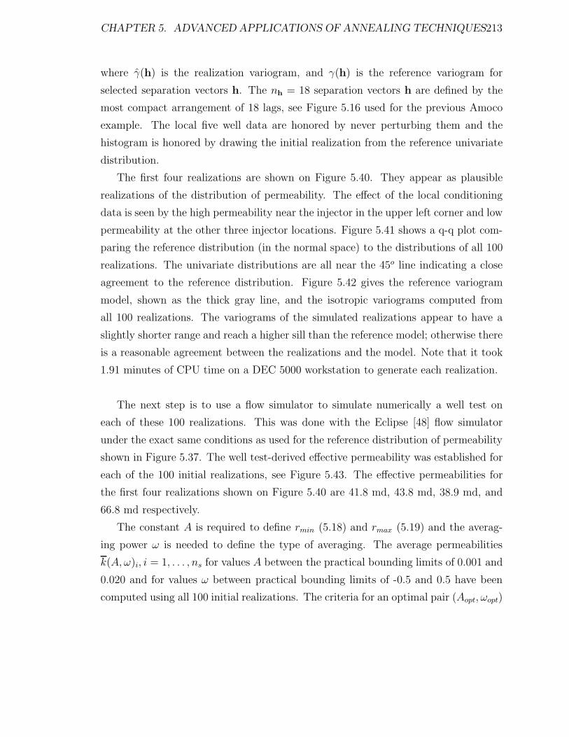
CHAPTER 5. ADVANCED APPLICATIONS OF ANNEALING TECHNIQUES213
where γ(h) is the realization variogram, and γ(h) is the reference variogram for
selected separation vectors h. The nh = 18 separation vectors h are defined by the
most compact arrangement of 18 lags, see Figure 5.16 used for the previous Amoco
example. The local five well data are honored by never perturbing them and the
histogram is honored by drawing the initial realization from the reference univariate
distribution.
The first four realizations are shown on Figure 5.40. They appear as plausible
realizations of the distribution of permeability. The effect of the local conditioning
data is seen by the high permeability near the injector in the upper left corner and low
permeability at the other three injector locations. Figure 5.41 shows a q-q plot com-
paring the reference distribution (in the normal space) to the distributions of all 100
realizations. The univariate distributions are all near the 45o line indicating a close
agreement to the reference distribution. Figure 5.42 gives the reference variogram
model, shown as the thick gray line, and the isotropic variograms computed from
all 100 realizations. The variograms of the simulated realizations appear to have a
slightly shorter range and reach a higher sill than the reference model; otherwise there
is a reasonable agreement between the realizations and the model. Note that it took
1.91 minutes of CPU time on a DEC 5000 workstation to generate each realization.
The next step is to use a flow simulator to simulate numerically a well test on
each of these 100 realizations. This was done with the Eclipse [48] flow simulator
under the exact same conditions as used for the reference distribution of permeability
shown in Figure 5.37. The well test-derived effective permeability was established for
each of the 100 initial realizations, see Figure 5.43. The effective permeabilities for
the first four realizations shown on Figure 5.40 are 41.8 md, 43.8 md, 38.9 md, and
66.8 md respectively.
The constant A is required to define rmin (5.18) and rmax (5.19) and the averag-
ing power ω is needed to define the type of averaging. The average permeabilities
k(A, ω)i, i = 1, . . . , ns for values A between the practical bounding limits of 0.001 and
0.020 and for values ω between practical bounding limits of -0.5 and 0.5 have been
computed using all 100 initial realizations. The criteria for an optimal pair (Aopt, ωopt)

CHAPTER 5. ADVANCED APPLICATIONS OF ANNEALING TECHNIQUES214
First Realization Second Realization
Third Realization Fourth Realization
Figure 5.40: The first four initial realizations generated with annealing. Note the effect ofthe five local conditioning data - one at each corner and the center.

CHAPTER 5. ADVANCED APPLICATIONS OF ANNEALING TECHNIQUES215
Q-Q Plot: Simulated versus Reference
Reference
Sim
ulat
ed
-4 -3 -2 -1 0 1 2 3
-4
-3
-2
-1
0
1
2
3
Figure 5.41: A q-q plot comparing the reference distribution (in the normal space) to thedistribution of all 100 realizations.
Normal Scores Semivariogram
Distance
Sem
ivar
iogr
am
0.0 5.0 10.0 15.0 20.0 25.0
0.0
0.2
0.4
0.6
0.8
1.0
1.2
Figure 5.42: A plot comparing the reference normal scores variogram (shown as the thickergray line) to variograms computed from all 100 realizations.

CHAPTER 5. ADVANCED APPLICATIONS OF ANNEALING TECHNIQUES216
Fre
quen
cy
20. 40. 60. 80. 100. 120.
.000
.040
.080
.120
Initial Realizations: Well Test-Derived Effective Permeabilitymean 58.30
std. dev. 15.45coef. of var 0.26
maximum 102.1upper quartile 70.8
median 54.6lower quartile 46.0
minimum 33.1
Figure 5.43: The histogram of 100 effective permeability values from initial realizations.
is to minimize the mean normalized absolute deviation and the mean normalized error
defined as:
NAD(A, ω) =i=ns∑i=1
|k(A, ω)i − ki|ki
(5.22)
NE(A, ω) = |∑i=ns
i=1 k(A, ω)i −∑i=nsi=1 ki∑i=ns
i=1 ki
| (5.23)
NAD measures correlation and NE measures the bias between the power average
approximation and the true well test values. Figure 5.44 shows gray level maps of
NAD and NE for values A ranging from 0.001 to 0.020 and values ω ranging from
-0.5 to 0.5. Note that the optimal pair Aopt = 0.003 and ωopt = 0.10 minimizes both
error terms.
Figure 5.45 shows a scatterplot of the power average numerical approximation and
the true well test-derived effective permeability. Note the unbiasedness (the average
effective permeabilities are 58.3 in both cases) and the excellent correlation value of
0.98. The physical volume informed by the well test can be determined from the
constant Aopt and knowledge of the time limits (tdminand tdmax):
rmin = A ·√
tdmin= 0.003 ·
√5.46x108 = 70.1feet

CHAPTER 5. ADVANCED APPLICATIONS OF ANNEALING TECHNIQUES217
a = 0.020
a = 0.010
a = 0.001w = -0.5 w = 0 w = +0.5
NAD
.0
.04
.08
.12
.16
.20
.24
.28
.32
.36
.40
a = 0.020
a = 0.010
a = 0.001w = -0.5 w = 0 w = +0.5
NE
.0
.04
.08
.12
.16
.20
.24
.28
.32
.36
.40
a = 0.020
a = 0.010
a = 0.001w = -0.5 w = 0 w = +0.5
NAD + NE
.0
.08
.16
.24
.32
.40
.48
.56
.64
.72
.80
Figure 5.44: Gray level maps of the mean normalized absolute deviation NAD, the meannormalized error NE, and the sum of NAD and NE, for A values ranging from 0.001to 0.020 and ω values ranging from -0.5 to 0.5. Note the optimal pair Aopt = 0.003 andωopt = 0.10 shown by the small circle.

CHAPTER 5. ADVANCED APPLICATIONS OF ANNEALING TECHNIQUES218
Pow
er A
vera
ge A
ppro
xim
atio
n
Well Test-Derived Effective Permeability
Approximate Permeability versus Well Test Derived Permeability
20. 40. 60. 80. 100. 120.
20.
40.
60.
80.
100.
120.
X Variable: mean 58.3variance 238.8
Y Variable: mean 58.3variance 290.3
correlation (r) 0.976rank correlation (r) 0.975
Figure 5.45: A scatterplot of the power average approximation and the true well test-derived effective permeabilities for all 100 initial realizations.
rmax = A ·√
tdmin= 0.003 ·
√113.8x108 = 320.0feet
The annular region defined by these limits are shown on Figure 5.46.
Conditioning to Well Test Permeability
Once the volume and type of averaging have been defined, the annealing program
developed in Chapter 3 sasim can be used to impose the power average (equation
5.17 with Aopt = 0.003 and ωopt = 0.1). The objective function is to match jointly
the spatial structure, as quantified by the variogram, and the well test derived per-
meability:
O = λ1
nh∑l=1
[γmodel(hl) − γrealization(hl)]2 + λ2
[kwelltest − krealization
]2(5.24)
The same 18 lags nh as considered for the initial 100 realizations were used for the
final simulations.
Figure 5.47 shows how each component in the objective function changes as the
simulation proceeds (the solid line is the deviation from the model variogram and

CHAPTER 5. ADVANCED APPLICATIONS OF ANNEALING TECHNIQUES219
Injector
Injector
Injector
Injector
Producer
Figure 5.46: An illustration of the annular region measured by the well test.
the dashed line is the deviation due to the well test permeability). Both component
objective functions go to zero at about 150,000 swaps. It took 1.7 minutes on a DEC
5000 to perform the 250,000 swaps (the far right of the horizontal scale on Figure 5.47)
needed to complete the simulation. It took 3.41 minutes of CPU time on a DEC 5000
workstation to generate each realization, versus 1.91 minutes of CPU time to generate
realizations that are not conditional to the well test. Once again, the temperature
reduction parameter λ in the annealing schedule could be lowered to decrease the
CPU time.
The first four realizations are shown on Figure 5.48. The conditioning data and
general characteristics (refer back to Figure 5.40) are still honored; now the calibrated
power average has also been imposed on the realizations.
Although the annealing approach imposes almost exactly the calibrated power
average, it does not ensure reproduction of either the actual effective permeability
of the actual field or the full pressure response. Another 100 well test flow simula-
tions are needed to establish the information brought by honoring the power average.
Figure 5.49 shows the distribution of the 100 well test derived effective permeability
values after post processing. Note that the distribution of effective permeabilities, af-
ter conditioning to the well test, is much more closely centered on the value inferred
from the reference image (41.1 md). Further, note the significant reduction in the
variance as compared to Figure 5.43.

CHAPTER 5. ADVANCED APPLICATIONS OF ANNEALING TECHNIQUES220
Objective Function versus Time
Number of swaps (1000’s)
Obj
ectiv
e F
unct
ion
0. 50. 100. 150. 200. 250.
.00
.20
.40
.60
.80
1.00
1.20
Figure 5.47: The objective function versus time for direct annealing simulation to matchvariogram (solid line) and the well test (dashed line).
The true reference value (41.1 md in this case) would be measured in practice and
the corresponding improvement in the distribution of effective permeabilities would
be accessible.
Impact on Output Uncertainty
The well test-derived effective permeability has been honored reasonably well by the
post-processed realizations. The important question addressed in this section is how
does integrating the well test-derived effective permeability impact the final reservoir
performance forecasting and the associated measure of uncertainty?
The impact of integrating the well test data is evaluated by simulating the perfor-
mance of the five spot pattern using the reference image (the truth), with the initial
realizations (without accounting for the well test data), and last with the realizations
conditional to the well test-derived effective permeability. The initially oil saturated
reservoir is produced by pumping from the central well and injecting water at the four
corner injector wells (see Figure 5.36). The following three output response variables
are recorded from the flow simulation output:

CHAPTER 5. ADVANCED APPLICATIONS OF ANNEALING TECHNIQUES221
First Well Test Conditioned Realization Second Well Test Conditioned Realization
Third Well Test Conditioned Realization Fourth Well Test Conditioned Realization
Figure 5.48: Four realizations of direct annealing simulation to match variogram and welltest.

CHAPTER 5. ADVANCED APPLICATIONS OF ANNEALING TECHNIQUES222
Fre
quen
cy
20. 40. 60. 80. 100. 120.
.000
.100
.200
.300
.400
Conditioned Realizations: Well Test-Derived Effective Permeabilitymean 92.0
std. dev. 3.26coef. of var 0.035
maximum 101.0upper quartile 94.0
median 92.2lower quartile 89.4
minimum 85.1
Figure 5.49: The histogram of 100 effective permeability values after post processing.
1. the time of first water arrival (breakthrough time),
2. the time to reach a 50% water cut,
3. and the final oil in place after a fixed period of production.
The three reference response values are:
Breakthrough time = 0.809 time units
Time to reach 50% water cut = 2.732 time units
Final oil recovery = 0.376
The problem is to assess the uncertainty related to prediction of these response
variables using only the five local conditioning data, the univariate distribution of
permeability values, the variogram, then in addition the well test result. Two hun-
dred additional flow simulations were performed on the initial and post-processed
realizations. Figure 5.50 shows the output space of uncertainty before and after con-
ditioning to the well test result. Table 5.5 shows the 95% probability interval before
and after conditioning to the well test data. The significant reduction in the width
of the 95% probability interval is the direct result of adding the well test-derived

CHAPTER 5. ADVANCED APPLICATIONS OF ANNEALING TECHNIQUES223
Response Variable 95% Probability Interval %q0.025 q0.5 q0.975 reduction
Breakthrough reference 1.46time before 0.45 1.11 2.15
after 0.63 1.28 2.16 -10%
Time to reach reference 5.5350% water cut before 2.22 4.12 7.36
after 3.14 4.66 6.83 -28%
Final oil reference 0.47recovery before 0.35 0.41 0.53
after 0.37 0.42 0.47 -44%
Table 5.5: Summary of output response results before and after conditioning to includethe well test-derived effective permeability.
effective permeability. Further, note that the central value (as characterized by the
median q0.5) of the post-processed realizations is closer to the true reference. Thus,
the output distributions of uncertainty are both more accurate and more precise after
accounting for more input data.
One should not expect perfect accuracy with only five well data even if the well
test data is used. In practice, the true reference value (shown as the black dot on
Figure 5.50) is not available and the width of a fixed probability interval, say the
95% probability interval, is used to assess the possible true response value. One
expects this assessment of uncertainty to be reduced as more relevant data such as
well test-derived properties are considered in the stochastic modeling.

CHAPTER 5. ADVANCED APPLICATIONS OF ANNEALING TECHNIQUES224
Fre
quen
cy
.00 .50 1.00 1.50 2.00 2.50
.000
.040
.080
.120
.160
Time of Water Breakthroughmean 1.17
std. dev. 0.42coef. of var 0.36
maximum 2.29upper quartile 1.39
median 1.11lower quartile 0.83
minimum 0.43
Fre
quen
cy
1.00 2.00 3.00 4.00 5.00 6.00 7.00 8.00 9.00
.000
.020
.040
.060
.080
Time to Reach 50 percent Water Cutmean 4.22
std. dev. 1.35coef. of var 0.32
maximum 7.97upper quartile 5.07
median 4.12lower quartile 3.14
minimum 1.76
Fre
quen
cy
.300 .350 .400 .450 .500 .550
.000
.020
.040
.060
.080
.100
Final Oil in Placemean 0.42
std. dev. 0.047coef. of var 0.11
maximum 0.55upper quartile 0.45
median 0.41lower quartile 0.38
minimum 0.34
Fre
quen
cy
.00 .50 1.00 1.50 2.00 2.50
.000
.050
.100
.150
.200
.250
Time of Water Breakthroughmean 1.2552
std. dev. .3562coef. of var .2838
maximum 2.1574upper quartile 1.3795
median 1.2804lower quartile 1.0201
minimum .6323
Fre
quen
cy
1.00 2.00 3.00 4.00 5.00 6.00 7.00 8.00 9.00
.000
.040
.080
.120
.160
Time to Reach 50 percent Water Cutmean 4.6369
std. dev. .8658coef. of var .1867
maximum 6.9745upper quartile 5.2162
median 4.6608lower quartile 4.0584
minimum 3.0233
Fre
quen
cy
.300 .350 .400 .450 .500 .550
.000
.050
.100
.150
.200
Final Oil in Placemean .4171
std. dev. .0237coef. of var .0568
maximum .4923upper quartile .4291
median .4156lower quartile .4017
minimum .3671
Figure 5.50: The simulated output distributions generated by the annealing realizationsbefore (left side) and after (right side) conditioning to the well test result. The upperhistograms are for the breakthrough time, the middle histograms are for the time to achievea 50% water cut, and the lower histograms are for final oil recovery. The black dot in thebox plot below each histogram is the true value obtained from the reference image, thethree vertical lines are the 0.025 quantile, the median (0.5 quantile), and the 0.975 quantileof the output distribution.

Chapter 6
Concluding Remarks
Reservoir performance forecasting calls for running flow simulators with numerical
models of the reservoir petrophysical properties (saturation, porosity, permeability,
. . . ). To yield unbiased predictions these numerical models must reflect both the
major flow units and the short scale heterogeneities [84]. The requirement to reflect
the short scale heterogeneities implies that smoothed models generated by kriging,
splines, or any conventional interpolation algorithm are inappropriate for reservoir
modeling. A stochastic simulation algorithm must be used to generate acceptable
input numerical models. The numerical models generated by stochastic simulation
algorithms are non-unique since the data spacing is typically large with respect to
the scale of these heterogeneities; there are many models which will honor both the
local conditioning data and the spatial variability.
Processing multiple stochastic models of the reservoir allows constructing an out-
put probability distribution of each critical response variable. For example, in an
enhanced oil recovery project a critical response variable could be the time at which
the flooding agent breaks through at the production wells. A probability distribution
of this time would be constructed by simulating the recovery project on a number
of stochastic reservoir models. These output distributions are used to judge the en-
gineering and economic viability of the project. A number of alternate production
scenarios could be considered to choose one that optimizes the ultimate recovery, with
minimal predicted uncertainty. Finally, once a production scenario has been chosen,
225

CHAPTER 6. CONCLUDING REMARKS 226
the stochastic models may be used for production planning and economic forecasting.
There are many techniques available for stochastic simulation. A recent article [59]
summarized seven different modeling techniques each of which could be implemented
in a number of different ways. The stochastic relaxation or annealing techniques
documented in this dissertation were not on the list. At the time of writing this
dissertation stochastic simulation is “the most vigorous sector of research and ap-
plications in geostatistics” [84] and new techniques are continually being developed.
Given the number of alternate techniques, criteria had to be developed to compare
simulation techniques. The following three criteria were proposed in Section 2.2:
1. A good technique must generate plausible realizations in a reasonable amount
of time. Time refers to the human involvement and CPU time required for the
initial set up and the repeated application of the technique.
2. A good technique is one that allows the maximum prior relevant information
to be accounted for. This is the only direct way to ensure that the output
distribution is as accurate as possible.
3. Finally, a good technique is one that explores the largest space of output un-
certainty, i.e., one that generates a maximum entropy distribution of response
variables.
These three criteria have been recalled and used in every chapter of this dissertation.
The motivation for considering annealing techniques arises from their ability to
integrate more prior information (see point 2 noted above) such as complex geolog-
ical structures and well test-derived effective properties. Chapter 3 of this disser-
tation developed the elements of an annealing-based stochastic simulation program
sasim that accounts for conventional covariance/variogram models, geological struc-
tures (through multiple-point statistics), and well test-derived effective permeabilities
(through appropriate power averages).
One concern with annealing-based techniques is that by exactly honoring control
statistics they may artificially limit the space of output uncertainty (see point 3 noted
above). Chapter 4 developed an extended example comparing stochastic simulation

CHAPTER 6. CONCLUDING REMARKS 227
based on annealing to the more conventional sequential Gaussian and sequential indi-
cator simulation techniques. It was shown that annealing actually generates a slightly
larger space of uncertainty. The reason for this was conjectured to be the very par-
ticular multivariate distributions used by the Gaussian and indicator techniques.
Following up on Chapter 3 and point 2 noted above, Chapter 5 presented some
advanced applications of annealing techniques where more prior information such
as multiple-point connectivity functions, seismic data, and well test-derived effective
properties were integrated into stochastic models. The importance of integrating
these additional data was displayed visually and quantified by output distributions
of flow-related variables. Integrating more relevant prior information leads to more
accurate and precise distributions of output uncertainty.
The research presented in this dissertation has uncovered many different ways
to improve the results obtained: 1) special coding and determining fast annealing
schedules would allow generating realizations much faster than the code given with
this dissertation, 2) many other types of engineering data, such as tracer tests, could
be integrated into stochastic models to yield even more accurate predictions, and 3)
accounting for uncertainty in the control statistics would lead to a larger space of
output uncertainty.
The original contribution of this dissertation has been the development of the
annealing algorithm for stochastic imaging in a reservoir modeling context. Anneal-
ing allows data, that conventional algorithms are incapable of accouting for, to be
integrated into stochastic models. The improvement in the accuracy and precision of
output distributions of uncertainty has been demonstrated with example applications
considering multiple-point spatial connectivity functions and well test data.
The immediate practical application of this technique is to stochastic modeling of
petroleum reservoirs and groundwater aquifers. The ability to integrate the results
of pressure transient well tests to integrate seismic data and to reproduce complex
geological patterns (geometries) will lead to better reservoir performance forecasting.

CHAPTER 6. CONCLUDING REMARKS 228
Ideas for Future Research
Most of the research needs discussed below may be related back to one of the three
criteria for a good stochastic simulation technique.
Implementation
The implementation of annealing for production use would warrant some effort to
fine tune the algorithm and reduce the CPU time requirements. For example, the
CPU time required to simulate the 1600 node Berea image was reduced by a factor
of 10 simply by adjusting the annealing schedule. Adjusting the annealing schedule
is problem specific since some problems require a slow schedule to arrive at plausi-
ble realizations. For example, a too fast cooling schedule can lead to artifact edge
effects. There is some evidence that analagous thermodynamic properties such as
the critical temperature [15], specific heat, or entropy [1] could be used to determine
automatically when the temperature can be decreased faster.
A number of odd artifacts, such as the checkerboard appearance of Figure 5.3,
were generated with certain objective functions. There is a need for flexible interac-
tive software that would allow real-time visualization of the stochastic model. For
example, the color frame buffer on workstation computers could be used as memory
for the simulated realization during the annealing simulation. In this way, the trans-
formation of a random image to a plausible stochastic model could be dynamically
visualized. It would be possible to appreciate which spatial features appear first and
how many components can practically enter the objective function. This visualization
would also help to understand better the annealing approach and would allow unre-
alistic realizations to be quickly recognized and discarded. One could interactively
modify the objective function with an immediate graphical display of the results.
The sasim code developed during the preparation of this dissertation should be
considered as the starting point for operating programs and further research.

CHAPTER 6. CONCLUDING REMARKS 229
Control Statistics
The annealing algorithm aims at reproducing specific control statistics. In many
cases it is not clear which statistics should be used and how to infer them. For
example, control patterns obtained by scanning reference geological images may be of
little practical value depending on the relationship between color or grayness and the
actual rock property being mapped. There are two other alternatives: 1) the result
of sedimentary clastic simulation [131] could be used to provide appropriate reference
images at the reservoir scale required, and 2) outcrops or detailed geological maps
constructed from zones of dense information could yield reference control patterns.
In all cases there is the risk that the control statistics may not be representative
of the actual reservoir; consequently, the distribution of output uncertainty may be
inaccurate. More research into the use of these real control patterns is warranted.
Any full assessment of uncertainty output should consider the uncertainty in the
input control statistics. Future research should address the problem of accounting for
uncertain control statistics in a number of ways. One possibility would be to consider
the control statistics as the result of some random function model. Then, prior to the
creation of a stochastic realization, the control statistics could be drawn from such
a model. The realizations would match the input statistics exactly and the space
of uncertainty would be expanded since these input statistics vary from one set of
realizations to another.
Engineering Data: Well Tests
One worthwile research avenue is the possibility of using engineering data based on a
convective process rather than a diffusive process. The pressure transient well tests
considered in this dissertation are based on a diffusive process; therefore, they are ap-
propriate for measuring average properties and are insensitive to local heterogeneities.
Measurements that depend on a convective process, such as tracer tests, would be
more suited to identifying local heterogeneities.
The well test information considered in this dissertation could also be extended

CHAPTER 6. CONCLUDING REMARKS 230
to multiple permeability averages within concentric annular volumes around the well-
bore. Alternate reservoir models such as fractured or faulted reservoirs could be
considered. For example, the positioning of fault boundaries could be formulated as
an optimization problem where the position and extent of the fault(s) is perturbed
to obtain a close match to an observed well test response.
Another interesting avenue of research opened up by this thesis work would be to
help in designing a test that would bring the most information about the reservoir. For
any given piece of data, as obtained from a particular well test, it should be possible
to judge its impact on output uncertainty before obtaining the information. This
would be done through stochastic simulation exercises similar to those documented
in Section 5.1 and Section 5.3. This would allow balancing the cost of obtaining
the data with its predicted impact on the output uncertainty. The data that most
significantly constrains the output realizations at the least cost is preferable.

Appendix A
Acquisition of Geological Images
This appendix documents the procedure used to acquire images in a format useful
for annealing and simulation applications. Real geological images, with all of their
complexity, motivate the development of stochastic simulation techniques that can
account for their characteristic yet complex features. The geological images here
considered correspond to clastic sedimentary environments. Clastic sediments are
the most important petroleum reservoir rock and present challenging characteristic
features for the methodology developed in this dissertation.
Depositional sedimentary environments can be classified from non-marine to deep
marine, i.e., according to topographic elevation starting from the mountains and
ending with deep sea fans.
Glacial Sediments are deposited directly from glacial ice. They are generally poorly
sorted and stratified and are rarely petroleum reservoir rocks (except in Oman).
Eolian Deposits originate from arid and semi-arid deserts. Most common are dune,
interdune, sand sheet, and extradune deposits. These are very important reser-
voir units and present considerable heterogeneity in the form of lateral discon-
tinuities, interspersed impermeable zones, cross-bedded units, and anisotropic
properties across individual laminae.
Alluvial Fan Deposits accumulate at the base of a mountain or other upland area.
These are not generally reservoir rocks for petroleum; however, some production
231

APPENDIX A. ACQUISITION OF GEOLOGICAL IMAGES 232
has been realized from ancient fan deltas in Texas, Oklahoma, New Mexico, and
Colorado.
Lacustrine Environments originate from lakes or lake systems. The major conti-
nental source of petroleum in North America, China, and North Africa is from
large lacustrine depositional systems.
Fluvial Facies Models are due to the activities of rivers, such as meandering,
straight, braided, and anastomosing environments. The coarse grained nature
of fluvial sediments form potentially good reservoir rocks. There are significant
corresponding petroleum deposits in Alberta, Montana, Texas, and Prudhoe
Bay which is largely an ancient braided river deposit.
Deltaic Environments result from interacting dynamic processes (wave energy,
tidal regime, currents, climate, . . . ) which modify and disperse riverborne flu-
vial clastic deposits. These are important reservoir source rocks.
Estuarine Deposits form in semi-enclosed marginal marine water (an estuary) where
the salinity is diluted from fluvial discharge. Estuarine deposits have excellent
oil and gas potential.
Tidal Flats occur on open coasts of low relief. The North Sea and Georgia coast of
the USA are important examples of tidal flats.
Barrier-Island and Strand Plain Deposits are sandy islands or peninsulas elon-
gated parallel to the shore. Strand-plains are wider in the land-sea direction
and generally lack well developed lagoons and inlets. These environments are
supplied and molded almost entirely by marine processes and are important oil
and gas reservoirs.
Continental Shelf is that part of the sea floor between the shoreline and the upper
edge of the continental slope. The potential for economic oil and gas accumu-
lations in sandstone facies of ancient shelf deposits is high.

APPENDIX A. ACQUISITION OF GEOLOGICAL IMAGES 233
Continental Slope is that part of the continental margin that has gradients of
greater than 1 in 40 (2.5%).
Submarine Fans are deep sea deposits formed by a whole family of mass flow pro-
cesses. Important petroleum sources are located in ancient submarine fan de-
posits (including nearly all the oil recovered in Southern California to date and
several areas within the North Sea Basin).
Each of these depositional environments is well documented in the literature. The
preceeding is to recall the origin of reservoirs and establish the important environ-
ments.
Another approach to classifying geological structures would be on the basis of the
process that creates a particular structure, e.g., structural, depositional, chemical.
This classification scheme was not considered because the above classification provides
better geometric information.
It is essential that the techniques developed in this dissertation apply to real
life problems. Consider the complexities shown on the geological images collected
later. These real images present characteristics that repeat themselves in space with
some variance; the random component makes the structures difficult to quantify with
marked point processes and the deterministic aspect of the structures poses problems
for the conventional stochastic simulation techniques.
Acquisition of Characteristic Features in an Electronic Format
Before discussing the detailed steps required to encode digitally a photograph, it is
worthwile to point out a prior fundamental assumption. The assumption is that the
rock properties are somehow characterized by a monotonic or known transform of the
grayness or color of the image. In many cases this assumption is not too limiting,
e.g., the shaleyness in a shaley-sandstone relates not only to the permeability of the
rock but also to its color. In other cases the color intensity or grayness may have no
relation to the petrophysical properties. Ideally, rock properties should be measured
directly at a very detailed scale as was done for the Berea sandstone example [53].
There are very few examples of this type of direct measurements; acquisition of such

APPENDIX A. ACQUISITION OF GEOLOGICAL IMAGES 234
exhaustive spatial data would have been prohibitively expensive for the purposes of
this dissertation.
When petrophysical properties are measured directly, a photograph or a geolo-
gist’s drawing can be digitally encoded by the procedure documented hereafter. One
significant limitation in the acquisition of geological features is that one must not to
violate any copyright protection. Permission to copy or scan an image is typically
obtainable from the publisher or original author/photographer. Some books com-
piled by educational facilities or geological associations grant limited permission to
make copies for non-commercial educational purposes, e.g., Sandstone Depositional
Environments [118]. Images from such sources have been used for this dissertation.
The procedure to encode digitally an image is:
1. The first step is to scan the image. A “Complete PC” [26] full page scanner was
purchased. The scanner will scan 8.5” by 11” pages at up to 256 gray scales and
at 300 dots per inch (dpi). Note that the gray scales are made up of particular
patterns of black pixels; the device will only scan black and white pixels at 300
dpi.
2. The scanner generates output files in a variety of commercial formats. The
difficulty is that all file formats are compressed and non-readable by standard
C or Fortran programs. Moreover, the compression algorithm is proprietary so
it is impossible to read the file directly.
This major hurdle (converting the format of the image) was crossed by using
the Microsoft Paintbrush program. The scanning software will write out a .pcx
format which the Paintbrush program can read. The Paintbrush program is
then used to write out a bit map file. This file is still binary but at least it
is not compressed. A C program was written to convert the binary file to files
compatible with the GSLIB programs [40].
3. It is now possible to read the file, create standard data files, and plot PostScript
gray scale or color maps. However, we are still not at a point where the image is
useful. The pixels are all black or white and the pattern indicates the grayness

APPENDIX A. ACQUISITION OF GEOLOGICAL IMAGES 235
Scanned Image
Figure A.1: Unprocessed output from the scanning program. Note the gray levels inducedby the pattern of black and white pixels.
level. Figure A.1 illustrates this on a small image (the original is less than one
inch square).
4. The next step is to measure the grayness by some moving window statistic
and replace the binary variable by a continuous variable. One example of this
is shown on Figure A.2 where the sum of blacks in a 3 by 3 pixel (black=1,
white=0) has replaced the original variable. Windows of various sizes, vary-
ing amounts of overlap, and varying weight functions (as described below) are
considered to remove artifacts. For example, Figure A.3 shows the image with
most artifacts removed.
The discontinuous 1/0 pixel measurements is converted to a continuous gray
scale measurement by applying a general inverse distance weighting scheme to
pixels falling within a neighborhood:
wi =
1(di+c)p∑n
i=11
(di+c)p
(A.1)
where, there are n pixels within the neighborhood, di is the anisotropic distance

APPENDIX A. ACQUISITION OF GEOLOGICAL IMAGES 236
Filtered Image
Figure A.2: Filtered with a 3 by 3 pixel sum of black pixels. Note that the pattern is lessgrainy relative to Figure A.1 but it still needs some artifacts removed.
Filtered Image
Figure A.3: Filtered so that most artifacts are removed.

APPENDIX A. ACQUISITION OF GEOLOGICAL IMAGES 237
from pixel i to the central pixel, c is a constant that smooths the weight function
(as c increases the weight function gets smoother), and p is another constant
that determines how fast the weight decreases with distance (as p increases the
weight decreases faster).
The concept of filtering or smoothing these types of images is discussed in
Switzer, 1983 [130]. A more extensive discussion on the importance of bound-
aries may be found in the same reference.
5. Sometimes the levels of grayness obtained from the moving windows are re-
combined to a subset of gray levels. There may be relatively few identifiable
classes. Considering the smallest number will simplify the analysis presented in
later chapters.
An Abbreviated Catalog of Geological Features
The following digitally encoded geological structures show characteristic features that
are not easily captured by two-points statistics. These images will motivate the de-
velopment of more advanced techniques and provide control patterns for statistical
analysis. These images do not represent an exhaustive illustration of clastic variabil-
ity. There are many other features that may be more important that those shown.
Note that some of the following images still show artifacts due to the scanning and
subsequent manipulation.
Figures A.4, A.5, A.6, and A.7 can generally be classified within the eolian en-
vironment. Figure A.4 is an example of characteristic cross bedding in an eolian
sandstone. Figure A.5 is an example of large-scale wedge and tabular cross strata
in an eolian environment (Zion National Park, Utah, U.S.A.). The photograph was
taken from A Study of Global Sand Seas [104]. Figure A.6 is an example of character-
istic ripple cross lamination structures. Figure A.7 is an example of migrating ripples
from the U.S. Wind Tunnel Laboratory.
Figures A.8 can generally be classified within the fluvial environment. Figure A.8
shows convoluted, deformed laminations in the upper part of a point bar of the Brazos
River, Texas.

APPENDIX A. ACQUISITION OF GEOLOGICAL IMAGES 238
Eolian Sandstone
Figure A.4: A real example of an eolian sandstone. The sandstone was cut into a thinrectangular parralelipiped (about 4 inches by 6 inches), photocopied, and then scanned at300 dpi to provide this image.
Wedge and Tabular Cross Strata
Figure A.5: An example of wedge and tabular cross strata (Zion National Park, Utah,U.S.A.) in an eolian sandstone (the image represents an exposed face of about 75 by 125feet). Photograph taken from A Study of Global Sand Seas [104].

APPENDIX A. ACQUISITION OF GEOLOGICAL IMAGES 239
Ripple Cross Lamination
Figure A.6: A core scale example of ripple cross laminations in an eolian sandstone.
Migrating Ripples
Figure A.7: An example of migrating ripples in a man-made eolian sandstone (Wind TunnelLaboratory).

APPENDIX A. ACQUISITION OF GEOLOGICAL IMAGES 240
Deformed Laminations
Figure A.8: A real example of convoluted and deformed laminations from a fluvial environ-ment. The original core photograph was copied from page 131 of Sandstone DepositionalEnvironments [118].
Figures A.9 and A.10 can generally be classified within a deltaic environment.
Figure A.9 shows lenticular sand laminations representing “starved current ripples”
common in the transition zone between the distal bar and distributary-mouth bar.
Figure A.10 shows large scale cross laminations common near the top of distributary-
mouth bar deposits.
Figure A.11 can generally be classified within an estuarine environment. Fig-
ure A.11 shows anastomosing layers of mud around sand ripples.
The inadequacy of two-points statistics is documented in chapter 2; however,
readers familiar with stochastic simulation techniques may have recognized that many
of the features documented in this section could not be reproduced with simulation
methods based on two-points or bivariate statistics.

APPENDIX A. ACQUISITION OF GEOLOGICAL IMAGES 241
Starved Current Ripples
Figure A.9: A real example of “Starved Current Ripples” from a deltaic environment. Theoriginal photograph was copied from page 162 of Sandstone Depositional Environments[118].

APPENDIX A. ACQUISITION OF GEOLOGICAL IMAGES 242
Large Scale Cross Laminations
Figure A.10: A real example of large-scale cross laminations from a deltaic environment.The original photograph was copied from page 162 of Sandstone Depositional Environments[118].
Anastomosing Mud Layers Around Sand
Figure A.11: A real example of anastomosing mud layers around sand ripples from anestuarine environment. The original photograph was copied from page 182 of SandstoneDepositional Environments [118].

Appendix B
Fluctuations in the cdf and
Variogram due to Ergodicity
Ergodicity is not a property of reality; it is a property of random function models.
The specific theoretical definition of ergodicity is not relevent for the applications
addressed in this appendix, it is enough to quote the ergodic characteristic theorem,
. . . Informally, a random process is said to be ergodic if the statistics of
a single realization of the process, observed over a finite spatial domain,
converge to their expected values as the size of the domain of observation
increases. G.R. Luster page 205 [99]
. . . The RF Z(u) is said to be “ergodic” in the parameter µ if the corre-
sponding realization statistics µ(l), ∀ realizations l, tends toward µ, as
the size of the field A increases. C.V. Deutsch and A.G. Journel page 121
[40]
The statistic or parameter µ is usually taken as the realization mean m =∫A z(u)du.
Ergodicity in the mean can be ensured if the covariance C(h) exists and tends to zero,
as h → ∞. Thus, if the covariance tends to zero (the variogram has a sill) and the
simulated field A becomes large with respect to the range of the covariance or vari-
ogram then the spatial mean mA of any one realization will converge to that of the
RF model.
243

APPENDIX B. FLUCTUATIONS IN THE CDF AND VARIOGRAM DUE TO ERGODICITY244
Although the notion of ergodicity can be applied to any statistic or combination
of statistics, e.g., the variogram itself, checking for ergodic conditions may not be
straightforward. To check convergence of a realization variogram requires knowledge
of fourth order moments, e.g., the fluctuation variance E{[γ(h) − γA(h)]2
}(p. 192
[90]), which are known only when the full spatial law is given by some analytical
model, e.g., the multivariate Gaussian model [134].
When one considers statistics based on any particular realization to infer the
model input statistics, one is implicitly assuming that the RF model considered is
ergodic in those statistics. In the practice of simulation, convergence is never fully
attained because realizations are simulated over finite fields, thus one should expect
fluctuations of the realization statistics from one realization to another. This appendix
provides an appreciation for the fluctuations that can be expected when the spatial
domain A is not large with respect to the range of correlation.
The statistics (histogram and variogram/covariance) of any one finite realization
will differ from the RF model or ensemble statistics. As the extent of the field gets
smaller the fluctuation of the realization statistics becomes greater.
Note that the important point is not the level of discretization. The size of the
field relative to the range of correlation is the important factor.
To illustrate this point consider a standard Gaussian RF model with a standard
normal histogram and an isotropic exponential covariance with effective range 25 grid
units (the a parameter is 25/3 = 8.3333):
C(h) =
[1 − exp(−h
a)
]
Two dimensional realizations, of varying size, are generated using the sgsim program
of GSLIB [40]. The fluctuation of the realization histogram and covariance/variogram
is observed for fields of different size. One hundred realizations of each size as specified
on Table B.1 were generated.
One hundred cumulative distribution functions for each of three selected grid sizes
(25, 100, and 250) are shown on Figure B.1. The one hundred isotropic variograms
for the same three selected grid sizes are shown on Figure B.2.

APPENDIX B. FLUCTUATIONS IN THE CDF AND VARIOGRAM DUE TO ERGODICITY245
Distributions (250 by 250 grid)
Reference N(0,1) Distribution
Rea
lizat
ion
Dis
trib
utio
ns
.00 .20 .40 .60 .80
.00
.20
.40
.60
.80
Distributions (100 by 100 grid)
Reference N(0,1) Distribution
Rea
lizat
ion
Dis
trib
utio
ns
.00 .20 .40 .60 .80
.00
.20
.40
.60
.80
Distributions (25 by 25 grid)
Reference N(0,1) Distribution
Rea
lizat
ion
Dis
trib
utio
ns
.00 .20 .40 .60 .80
.00
.20
.40
.60
.80
Figure B.1: P-P plots for 100 realizations of three different grid sizes.

APPENDIX B. FLUCTUATIONS IN THE CDF AND VARIOGRAM DUE TO ERGODICITY246
Variograms (250 by 250 grid)
Distance (grid units)
Var
iogr
am .0 5.0 10.0 15.0 20.0 25.0
.00
.40
.80
1.20
1.60
Variograms (100 by 100 grid)
Distance (grid units)
Var
iogr
am
.0 5.0 10.0 15.0 20.0 25.0 .00
.40
.80
1.20
1.60
Variograms (25 by 25 grid)
Distance (grid units)
Var
iogr
am
.0 5.0 10.0 15.0 20.0 25.0 .00
.40
.80
1.20
1.60
Figure B.2: Variograms for 100 realizations of three different grid sizes.

APPENDIX B. FLUCTUATIONS IN THE CDF AND VARIOGRAM DUE TO ERGODICITY247
Grid Size Relative Number of Nodes perSize Realization
500 20 250,000250 10 62,500150 6 22,500100 4 10,00075 3 5,62550 2 2,50025 1 625
Table B.1: The grid sizes considered to evaluate the ergodic fluctuations in the histogramand variogram. The size is given relative to the effective range (25).
As expected, the fluctuations in all three cases are centered around the model
statistics, i.e., there is no systematic bias. Also, as expected, there is significantly
more fluctuation for the 25 by 25 field than for the larger 250 by 250 field.
The fluctuation of the realization statistics from the model statistics could be
quantified by any measure of dispersion (e.g., the fluctuation variance as described
in Luster p. 192 [99]). One common, easily understood, measure of dispersion is the
mean absolute deviation:
mADcdf =1
nr
1
nc
nr∑i=1
nc∑j
|cdfmodel(j) − cdfrealization(i, j)| (B.1)
mADvariogram =1
nr
1
nlag
nr∑i=1
nlag∑j
|γmodel(j) − γrealization(i, j)| (B.2)
for nr realizations, nc cdf cutoffs, and nlag lags. In the present case there are 100
realizations (nr = 100), 9 deciles considered (nc = 9), and 24 lags (nlag = 24).
The mAD measure of spread was chosen over the more traditional variance measure
because it is expressed in the unit of the statistics being considered. The mAD
measure of dispersion for both the CDF and the variogram have been plotted versus
the relative size of the simulated field (relative to the effective range of correlation)
on Figures B.3 and B.4.
Comments:

APPENDIX B. FLUCTUATIONS IN THE CDF AND VARIOGRAM DUE TO ERGODICITY248
mAD of Simulated Variogram from Model Variogram
Size of Simulations (relative to range)
mA
D
.0 5.0 10.0 15.0 20.0 25.0 .000
.050
.100
.150
.200
Figure B.3: mAD of the Gaussian realization cdfs from the model cdfs.
mAD of Simulated Variogram from Model Variogram
Size of Simulations (relative to range)
mA
D
.0 5.0 10.0 15.0 20.0 25.0 .000
.050
.100
.150
.200
Figure B.4: mAD of the Gaussian realization variograms from the model variograms.

APPENDIX B. FLUCTUATIONS IN THE CDF AND VARIOGRAM DUE TO ERGODICITY249
• The fluctuations in the cdf and the variogram appear to decrease at the same
rate, e.g., the decrease in the mAD from a field the size of the range to that
10 times the range is 33% and 28% for the cdf and variogram respectively. It
is interesting to note that the bivariate statistics converge at the same rate or
faster than the univariate statistics.
• Note that the number of nodes is the size of the simulation squared, e.g., four
times the number of nodes must be simulated to double the size of the real-
izations. In fact, the increase is a function of dimension being considered; the
increase would be cubic for 3-D simulations.
• Fluctuations in the cdf can be removed by resetting the quantiles of the distri-
bution (see Isaaks and Srivastava [69], p. 469).
The multivariate Gaussian model is notable for its congenial properites (see Chap-
ters 2 and 4). It was conjectured that the fluctuations will be greater for any other
random function model. The median IK model (see Chapter 2), which may be used
to simulate realizations with the same univariate distribution and variogram, was
considered to test this conjecture. One hundred cumulative distribution functions
for the same three grid sizes (25, 100, and 250) are shown on Figure B.5. The one
hundred omnidirectional variograms for the same three selected grid sizes are shown
on Figure B.6.
The mAD dispersion of the realization cdfs from the model and the realization
variograms from the model are shown on Figures B.7 and B.8. These can be com-
pared to those for the Gaussian RF model shown on Figures B.3 and B.4 which are
reproduced in the gray dashed line on Figures B.7 and B.8.
The fluctuations in the cdf and the variogram appear significantly higher than
those for the Gaussian RF model. These ergodic fluctuations serve to expand the
sampled space of uncertainty and could be considered a good property (see Section
2.2).

APPENDIX B. FLUCTUATIONS IN THE CDF AND VARIOGRAM DUE TO ERGODICITY250
Distributions (250 by 250 SIS grid)
Reference N(0,1) Distribution
Rea
lizat
ion
Dis
trib
utio
ns
.00 .20 .40 .60 .80
.00
.20
.40
.60
.80
Distributions (100 by 100 SIS grid)
Reference N(0,1) Distribution
Rea
lizat
ion
Dis
trib
utio
ns
.00 .20 .40 .60 .80
.00
.20
.40
.60
.80
Distributions (25 by 25 SIS grid)
Reference N(0,1) Distribution
Rea
lizat
ion
Dis
trib
utio
ns
.00 .20 .40 .60 .80
.00
.20
.40
.60
.80
Figure B.5: P-P plots for 100 realizations of three different grid sizes.

APPENDIX B. FLUCTUATIONS IN THE CDF AND VARIOGRAM DUE TO ERGODICITY251
Variograms (250 by 250 SIS grid)
Distance (grid units)
Var
iogr
am .0 5.0 10.0 15.0 20.0 25.0
.00
.40
.80
1.20
1.60
Variograms (100 by 100 SIS grid)
Distance (grid units)
Var
iogr
am
.0 5.0 10.0 15.0 20.0 25.0 .00
.40
.80
1.20
1.60
Variograms (25 by 25 SIS grid)
Distance (grid units)
Var
iogr
am
.0 5.0 10.0 15.0 20.0 25.0 .00
.40
.80
1.20
1.60
Figure B.6: Variograms for 100 realizations of three different grid sizes.
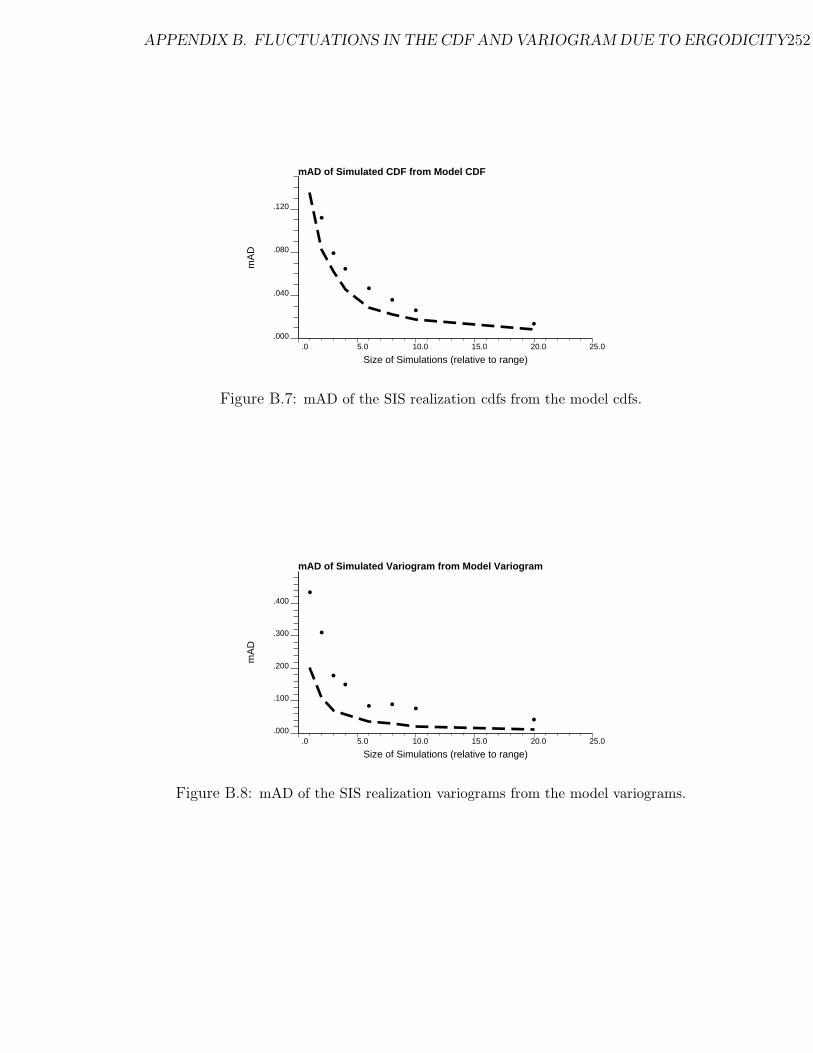
APPENDIX B. FLUCTUATIONS IN THE CDF AND VARIOGRAM DUE TO ERGODICITY252
mAD of Simulated CDF from Model CDF
Size of Simulations (relative to range)
mA
D
.0 5.0 10.0 15.0 20.0 25.0 .000
.040
.080
.120
Figure B.7: mAD of the SIS realization cdfs from the model cdfs.
mAD of Simulated Variogram from Model Variogram
Size of Simulations (relative to range)
mA
D
.0 5.0 10.0 15.0 20.0 25.0 .000
.100
.200
.300
.400
Figure B.8: mAD of the SIS realization variograms from the model variograms.

Appendix C
A Detailed Look at Spatial Entropy
As of 1992 the vast majority of geostatistical estimation (prediction) and stochastic
simulation algorithms rely on a covariance model as the sole characteristic of the
spatial distribution of the attribute under study. The choice of the covariance im-
plicitly calls for a multivariate Gaussian model for either the attribute itself or for
its normal scores transform. The choice of a prior Gaussian model could be justified
on the basis that it is both analytically simple and it is a maximum entropy model,
i.e., a model that minimizes unwarranted prior information1. The Gaussian maxi-
mum entropy characteristic also entails maximization of spatial disorder (beyond the
imposed covariance) which may cause flow simulation results performed on multiple
stochastic images to be very similar; thus, the space of (posterior) uncertainty could
be too narrow entailing a misleading sense of safety. The ability of the sole covariance
to describe adequately spatial distributions for flow studies, and the assumption that
maximum spatial disorder amounts to either no information or a safe prior hypothesis
are questioned.
This appendix attempts to clarify the link between entropy and spatial disorder
and to provide, through some examples, an appreciation of the impact of entropy of
prior random function models on the resulting response distributions.
Although extensively used in thermodynamics and information theory [58, 74, 96,
120] the concept of entropy has only been recently introduced in geostatistics [24, 116].
1That is, information that is an artifact of the RF model and not true data.
253

APPENDIX C. A DETAILED LOOK AT SPATIAL ENTROPY 254
Entropy is a measure of the uncertainty of a prior distribution model; the principle
is to maximize the uncertainty (entropy) beyond the statistics that are considered
known. In other words, the prior random function model should account only for the
statistics deemed known. If those statistics reduce to the covariance function, it is
known that the maximum entropy random function model is Gaussian. Whenever
enough data are available to allow inference of a covariance model they also usually
provide valuable additional information; in which case the maximum entropy prior
random function model is no longer Gaussian.
A case-study will show that alternative prior random function models sharing the
same covariance model could lead to much larger (posterior) uncertainty in the re-
sponse variables of transport simulations, such as effective permeability, breakthrough
times, or oil/water sweepage.
C.1 Entropy of Continuous Distributions
Let fz = fz(z1, z2, . . . , zn) be the n-variate probability density function (pdf) of the
n random variables (RV’s) Zi, i = 1, . . . , n. The uncertainty associated to the distri-
bution fz is measured by its entropy defined as [119, 24]:
Hfz = E {−lnfz(z1, . . . , zn)} (C.1)
= −∫ +∞
−∞. . .
∫ +∞
−∞[lnfz(z1, . . . , zn)] fz(z1, . . . , zn)dz1, . . . , dzn
Since the posittive function −ln(y) increases as y decreases, the smaller the pdf value
fz(z1, . . . , zn) the larger its contribution to the entropy measure H . The greater the
uncertainty, the more spread and the smaller the pdf values fz, the larger the entropy.
Note that entropy is unit-free.
The logarithmic function ln(y) comes from thermodynamics and statistical physics
where it naturally arises from the Boltzmann distribution.

APPENDIX C. A DETAILED LOOK AT SPATIAL ENTROPY 255
Univariate pdf:
For n = 1, relation (C.1) defines the entropy of a univariate continuous distribution
with pdf f(z):
Hf = −∫ +∞
−∞[lnf(z)] f(z)dz (C.2)
Classical results include, Shannon and Jones [119, 74].
• The bounded pdf with maximum entropy is the uniform distribution, i.e., f(z) =1
b−afor z ∈ [a, b] and f(z) = 0 otherwise. The entropy is Hf = ln(b − a) which
decreases to −∞ as the interval [a, b] becomes narrower corresponding to greater
certainty.
• The maximum entropy unbounded pdf 2 with a fixed variance is the normal
(Gaussian) distribution independent of its mean or expected value.
Bivariate pdf:
For n = 2, or for two RV’s Z(u) and Z(u + h) separated by a given vector h, the
entropy associated to the bivariate pdf fh(z, z′) is:
Hf(h) = −∫ +∞
−∞
∫ +∞
−∞[lnfh(z, z′)] fh(z, z′)dzdz′ (C.3)
The previous univariate results extend to the bivariate case:
• For bounded RV’s, maximum entropy is obtained for the uniform or rectangular
bivariate pdf.
• Among all bivariate pdf’s sharing the same covariance function
C(h) = Cov{Z(u), Z(u + h)} or the same covariance matrix E{(Z − m)(Z −m)T}, the Gaussian pdf maximizes entropy. Thus, if the only prior structural
information (spatial statistics) retained is the covariance function C(h) the
maximum entropy RF model is the Gaussian model.
2In practice, most histograms are bounded and very few can be considered as normal. However,a normal score transform can be applied (p. 478 [90]), and the previous argument holds for thenormal pdf of the transforms.

APPENDIX C. A DETAILED LOOK AT SPATIAL ENTROPY 256
• Different bivariate pdf’s may share the same covariance C(h) and yet have
different entropy functions Hf(h).
C.2 Entropy of Discrete Distributions
The integral expressions (C.2) and (C.3) of entropy call for continuous pdf’s and are
usually only used for analytical developments. In most practical applications, the
variable Z(u) is either categorical (e.g., rock types) or, if continuous, is discretized
into a finite number of classes, e.g., the classes of its histogram.
Let Z be a discrete RV that can take K outcome values (or be valued in K
predefined classes) with probabilities pk, k = 1, . . . , K, such that∑K
k=1 pk = 1.
The entropy attached to this discrete probability set is defined as:
H = −K∑
k=1
[lnpk]pk ≥ 0 (C.4)
Similarly, consider the stationary discrete RF Z(u) with for stationary marginal
probabilities the set {pk, k = 1, . . . , K}, and for bivariate probabilities the set:
pk,k′(h) = Prob{Z(u) ∈ category k, Z(u + h) ∈ category k′}independent of u; k, k′ = 1, . . . , K (C.5)
Note that∑K
k′ pk,k′(h) = pk = Prob{Z(u) ∈ category k} for all h.
The entropy associated to that set of bivariate probabilities is defined as:
H(h) = −K∑
k=1
K∑k′=1
[lnpk,k′]pk,k′ ≥ 0 (C.6)
Recall: [lnp]p → 0, as p → 0.
Some additional remarks:
• The discrete case entropy is non-negative as compared to the continuous case
where the entropy can be as low as −∞ (because the density fZ(z) can be
greater than 1).

APPENDIX C. A DETAILED LOOK AT SPATIAL ENTROPY 257
• If the RV Z(u) is not naturally categorical but is made discrete through clas-
sification, the class definition impacts the entropy value as defined in relations
(C.4) or (C.6). Hence, before comparing the discrete entropies of originally con-
tinuous distributions, care should be taken to standardize the class definition.
• For lag h = 0 : pk,k′(0) = 0, ∀k �= k′, and: pkk(0) = pk. Thus, the definition (6)
entails:
H(0) = −K∑
k=1
[lnpk]pk ≡ H (C.7)
The univariate entropy represents the lower bound of the bivariate entropy, i.e.,
H(h) ≥ H(0), ∀h. This lower bound can be seen as the case corresponding to
perfect dependence: Z(u + h) ≡ Z(u).
• For lag h = +∞, the two very distant RV’s Z(u) and Z(u+h) are independent
from each other, hence:
pk,k′(+∞) = pkpk′, ∀k, k′
and from relation (6):
H(∞) = −K∑
k=1
K∑k′=1
[lnpk + lnpk′] pkpk′
= −K∑
k=1
lnpk
K∑k′=1
pk′ −K∑
k′=1
lnpk′K∑
k=1
pk = 2H(0)
H(∞) = 2H(0) (C.8)
Therefore, the bivariate entropy is bounded below by the univariate entropy H(0)
and above by twice the univariate entropy:
H(h) ∈ [H(0), 2H(0)] (C.9)
Thus, a standardized relative measure of bivariate entropy is:
HR(h) =H(h) − H(0)
H(0)∈ [0, 1] (C.10)

APPENDIX C. A DETAILED LOOK AT SPATIAL ENTROPY 258
This measure of spatial disorder is compared with the relative semi-variogram defined
as (p. 33 [90]):
γR(h) =1
2
E {[Z(u + h) − Z(u)]2}C(0)
=C(0) − C(h)
C(0)∈ [0, 1] (C.11)
with C(h) being the covariance function Cov{Z(u), Z(u + h)} and C(0) the corre-
sponding variance.
The relative bivariate entropy (C.10) allows comparison of the spatial distribution
of two discrete RF’s Z(u) and Y (u) with different histograms.
C.3 Spatial Entropy
Building on the similarity of the two expressions (C.10) and (C.11) one can define an
average bivariate entropy over a field A of measure |A| as:
HR(A, A) =1
|A|2∫
Adu
∫A
HR(u − u′)du′ ∈ [0, 1] (C.12)
In practice the field A would be discretized by n locations of coordinates ui,
i = 1, . . . , n, and the space integral (C.12) approximated by:
HR(A, A) ∼= 1
n2
n∑i=1
n∑j=1
HR(ui − uj) (C.13)
When A → ∞, HR(A, A) → 1, since HR(∞) → 1.
Expressions (C.12) and (C.13) are similar to the expressions defining the dispersion
(expected spatial) variance of Z(u) within the field A, (p. 67 [90]):
D2(0/A) = E{S2(0/A)} = γ(A, A) =1
|A|2∫
Adu
∫A
γ(u − u′)du′ (C.14)
with S2(0, A) being the randomization of the spatial variance
s2(0, A) =1
|A|∫
A[z(u) − mA]2du and mA =
1
|A|∫
Az(u)du
The average relative entropy measure HR(A, A), defined in (C.12) could be used as a
global measure of spatial entropy (disorder) over the field A. However, whether this

APPENDIX C. A DETAILED LOOK AT SPATIAL ENTROPY 259
measure will prove more useful than the little used dispersion variance (C.14) is yet
questionable.
Note that the measure HR(A, A) utilizes only bivariate entropy when a full mea-
sure of the spatial entropy should use all multivariate entropy functions. In practice,
multivariate pdf’s are inaccessible. Similarly, multivariate entropy functions are not
likely to be accessible.
C.4 Some Examples
The visual difference between the low and high spatial entropy cases in the following
examples is easily appreciated; however, it is more important to demonstrate that
there is a significant effect on the response variables. Such demonstration has been
given in [87] and in chapter 4.
C.4.1 A Discrete Variable Example
Figure C.1 shows two realizations of a 2-D bombing model, i.e., circles of a constant
diameter a with their centers located in space by a Poisson process. An indicator
I(u) is defined as 0 if the point at location u falls within a circle and 1 if it falls
outside. The variogram for this process can be calculated analytically as [102, 122].
γ(h) = p(1 − pCirca(|h|))
where, h is the separation vector of modulus |h|, a is the diameter of the circles, p is
the fraction outside the circles, (1 − p) is the fraction within the circles, p(1 − p) is
the variance of the indicator I(u), and Circa(h) is the circular variogram model:
Circa(h) =
2πa2
[|h|√
a2 − |h|2 + a2sin−1( |h|
a
)], |h| ≤ a
1, |h| ≥ a
This indicator variogram model γ(h) has the familiar p(1−p) variance form with the
exponent corresponding to the hyperspherical variogram model for the dimension of
the space being considered. In 1-D the exponent becomes the linear variogram up

APPENDIX C. A DETAILED LOOK AT SPATIAL ENTROPY 260
Figure C.1: Two realizations of a 2-D bombing model.
to the range a; in 2-D the exponent is the circular variogram model; and in 3-D the
exponent becomes the spherical variogram model.
All of the realizations shown hereafter feature p = 68%±1%. That is, all simulated
indicator realizations have about the same mean and variance.
Figure C.2 shows both the analytical model and the omnidirectional experimental
variograms computed from the two realizations shown on Figure C.1. Note that the
range of the variogram is 20 units (the diameter of the circles) and the size of the
simulated field is 200 units by 200 units, ensuring reasonable ergodicity.
The bombing model images have a very low entropy for the given variogram
model. It is conjectured that these images are minimum entropy realizations for this
variogram.
Realizations generated from a multiGaussian random function model have the
maximum spatial entropy for any given covariance model. A sequential Gaussian
simulation algorithm [40, 56] has been employed to create two realizations that match
the analytical variogram model of the previous 2-D bombing model process, see Fig-
ure C.3. The corresponding omnidirectional experimental variograms and the ana-
lytical model are shown on Figure C.4.
An alternative to the maximum entropy Gaussian RF model is the implicit an-
nealing RF model which remains poorly understood. Two realizations that match
the variogram of the 2-D bombing model process are shown on Figure C.5 and the

APPENDIX C. A DETAILED LOOK AT SPATIAL ENTROPY 261
Var
iogr
am
Distance
Variograms for Bombing Model Realizations
.0 10.0 20.0 30.0 40.0 50.0
.000
.050
.100
.150
.200
Figure C.2: The analytical variogram model and the variogram corresponding to the twoimages shown on Figure C.1.
Figure C.3: Two realizations of a multiGaussian random function model with the variogramof a 2-D bombing model process. For that variogram these are maximum spatial entropyrealizations.
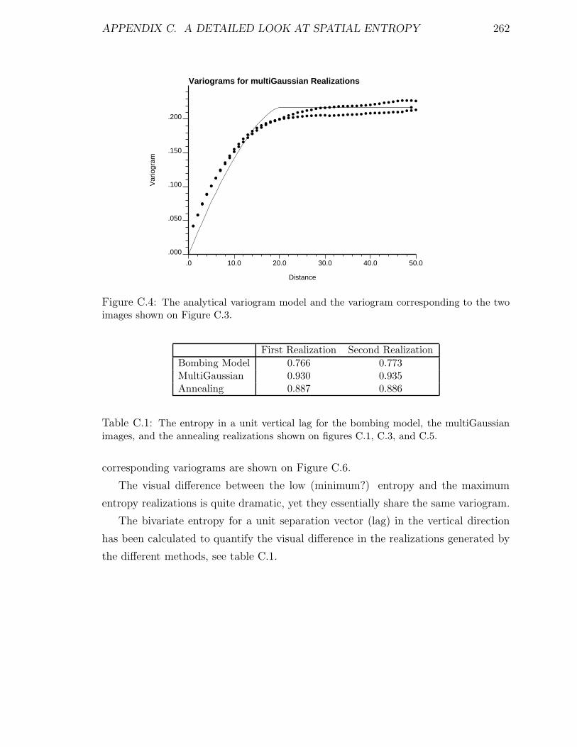
APPENDIX C. A DETAILED LOOK AT SPATIAL ENTROPY 262
Var
iogr
am
Distance
Variograms for multiGaussian Realizations
.0 10.0 20.0 30.0 40.0 50.0
.000
.050
.100
.150
.200
Figure C.4: The analytical variogram model and the variogram corresponding to the twoimages shown on Figure C.3.
First Realization Second RealizationBombing Model 0.766 0.773MultiGaussian 0.930 0.935Annealing 0.887 0.886
Table C.1: The entropy in a unit vertical lag for the bombing model, the multiGaussianimages, and the annealing realizations shown on figures C.1, C.3, and C.5.
corresponding variograms are shown on Figure C.6.
The visual difference between the low (minimum?) entropy and the maximum
entropy realizations is quite dramatic, yet they essentially share the same variogram.
The bivariate entropy for a unit separation vector (lag) in the vertical direction
has been calculated to quantify the visual difference in the realizations generated by
the different methods, see table C.1.
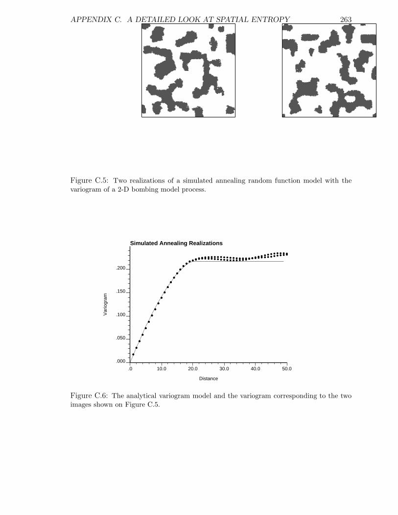
APPENDIX C. A DETAILED LOOK AT SPATIAL ENTROPY 263
Figure C.5: Two realizations of a simulated annealing random function model with thevariogram of a 2-D bombing model process.
Var
iogr
am
Distance
Simulated Annealing Realizations
.0 10.0 20.0 30.0 40.0 50.0
.000
.050
.100
.150
.200
Figure C.6: The analytical variogram model and the variogram corresponding to the twoimages shown on Figure C.5.

APPENDIX C. A DETAILED LOOK AT SPATIAL ENTROPY 264
C.4.2 A Continuous Variable Example
The so-called “mosaic” model is a bivariate mixture of two binormal distributions
with common univariate Gaussian distribution. The first binormal distribution has a
correlation coefficient of 1 (i.e., all values are equal) and the second binormal distri-
bution has a correlation coefficient of 0 (i.e., all values are independent). A mixture of
these two Gaussian distributions with proportion p(h) yields the following “mosaic”
bivariate distribution [101, 77]:
Fh(z, z′) == Prob{Z(u) ≤ z; Z(u+h) ≤ z′} = p(h)F (min(z, z′))+[1 − p(h)] F (z)F (z′)
where z corresponds to Z(u) and z′ corresponds to Z(u+h). Thus, the mosaic model
corresponds to a random function model such that Z(u) and Z(u+h) are equal with
probability p(h) and independent with the complement probability [1 − p(h)].
For a given covariance, the mosaic model has low spatial entropy: its realizations
will appear as a mosaic of independent patches of constant values, see Figure C.7.
A second interesting property of the mosaic model is that indicator correlograms
do not tend towards a pure nugget effect as the cutoff departs symmetrically from
the median, as would be the case for all multiGaussian related models [77], includ-
ing the multilognormal model. In fact, the mosaic indicator correlograms and cross
correlograms are all equal, independently of the cutoff. Therefore, realizations of
this random function model may be obtained by median indicator kriging [77] and
simulation [83]. The median indicator approach corresponds to the case when the
variogram inferred from the median cutoff is used for all other cutoffs. Consequently,
the indicator kriging weights are identical for all cutoffs.
Two realizations of a 200 by 200 unit square area are shown on Figure C.7; they
correspond to a mosaic mixture of two multilognormal distributions. The common
univariate distribution is lognormal with a mean of 1.65 and a variance of 4.67. All
indicator variograms and the normal scores variogram are exponential with no nugget
effect and a practical range of 21 units (3 times the integral range 7):
γ(h) = 1 − e−|h|
7
Figure C.8 shows the analytical and the corresponding omnidirectional experimental

APPENDIX C. A DETAILED LOOK AT SPATIAL ENTROPY 265
.0
1.00
2.0
3.0
4.0
5.0
6.0
7.0
8.0
9.0
10.0
.0
1.00
2.0
3.0
4.0
5.0
6.0
7.0
8.0
9.0
10.0
Figure C.7: Two realizations of the mosaic model generated by median indicator simula-tion.
First Realization Second RealizationMosaic Model 3.480 3.460MultiGaussian 3.670 3.677
Table C.2: The entropy in a unit vertical lag for the mosaic model and multiGaussianimages shown on figures C.7 and C.9.
variograms for the normal scores variable.
Two maximum entropy counterparts with the same univariate lognormal distribu-
tion and normal scores variogram are shown on Figure C.9. These realizations were
generated with the sequential Gaussian simulation algorithm [83]. The analytical and
experimental variograms are shown on Figure C.10.
The significant visual difference between these two random function models may
be quantified by the bivariate entropy for a unit lag in the vertical direction shown
on table C.2.
C.5 Final Thoughts
The Gaussian RF model presents maximum spatial entropy and disorder beyond the
imposed covariance; this does not imply, however, that critical response variables

APPENDIX C. A DETAILED LOOK AT SPATIAL ENTROPY 266
Var
iogr
am
Distance
Normal Scores Variograms
.0 10.0 20.0 30.0 40.0 50.0
.00
.20
.40
.60
.80
1.00
1.20
Figure C.8: The analytical variogram model and the variogram corresponding to the twoimages shown on Figure C.7.
.0
1.00
2.0
3.0
4.0
5.0
6.0
7.0
8.0
9.0
10.0
.0
1.00
2.0
3.0
4.0
5.0
6.0
7.0
8.0
9.0
10.0
Figure C.9: Two realizations of a multilognormal random function model with the vari-ogram of the median indicator simulation realizations of Figure C.8. These are maximumspatial entropy realizations.

APPENDIX C. A DETAILED LOOK AT SPATIAL ENTROPY 267
Var
iogr
am
Distance
Normal Scores Variograms
.0 10.0 20.0 30.0 40.0 50.0
.00
.20
.40
.60
.80
1.00
1.20
Figure C.10: The analytical variogram model and the variogram corresponding to the twoimages shown on Figure C.9.
from some transfer function will present the same maximum entropy character. In
fact, for some transfer functions, the Gaussian maximum entropy model may entail a
too narrow and non-conservative assessment of output uncertainty (see Sections 4.5
and 5.2.2).

Appendix D
Kriging in a Finite Domain
Adopting a random function (RF) model {Z(u),u ∈ study area A} and using the
normal equations (kriging) for estimation amounts to assume that the study area A is
embedded within an infinite domain. At first glance, this assumption has no inherent
limitations since all locations outside A are of no interest and simply not considered.
There is an interesting and practically important consequence that is reflected in
the kriging weights assigned to data contiguously aligned along finite strings. This
appendix, which documents this feature of the normal equations or kriging, is relevant
since that feature affects the quality of realizations generated with the conventional
random function (RF) approach and is not documented in any known publication.
Recall that the posterior conditional cumulative distribution functions (ccdf’s)
needed for stochastic simulation are established by constructing linear combinations
of nearby data values (or specific non-linear transforms of the original data values,
see section 2.3). Simple kriging is the theoretically correct algorithm to arrive at the
weights for each linear combination1. In practice, the more robust ordinary kriging
is often used to filter the global stationary mean from the linear combination.
Figure D.1 shows two commonly encountered situations where finite strings of
contiguously aligned data are used in kriging. In the first case, when strings of
measurements taken along a borehole are truncated by geological or stratigraphic
1This is true for the multiGaussian and the indicator RF models - two of the most common RFmodels used in practice.
268

APPENDIX D. KRIGING IN A FINITE DOMAIN 269
Kriging Within Stratigraphic Limits
drillhole
drillholedrillhole
Kriging Within a Local Search Neighborhood
?
drillhole
drillhole
drillhole
Figure D.1: Two commonly encountered situations when finite strings of contiguouslyaligned data are used in kriging. In the top figure the shaded area represents a stratigraphiclayer of interest. The shaded area in the bottom figure represents the limits of a local searchneighborhood.
APPENDIX D. KRIGING IN A FINITE DOMAIN 270
boundaries, the study area A is clearly finite. In the second case, when strings of
data are truncated by the boundaries of a local search ellipsoid, the area A may be
infinite but the local neighborhood is not.
Figure D.2 illustrates the counter-intuitive weighting scheme that will result when
kriging with a finite string of data. The profile of the ordinary kriging weights is shown
next to the string. The variogram is a common spherical model with a range equal
to the length of the string. Note that the point being estimated is beyond the range
of the variogram and yet the implicit declustering of kriging causes the weights to
change considerably along the vertical extent of the string with the outermost samples
receiving a disproportionately large weight. Further note that the kriging weights will
remain unchanged as the point being estimated moves further away. Kriging yields
this type of weighting because of the implicit assumption that the data are within an
infinite domain - the outermost data inform the infinite half-space beyond the data
string and hence receive greater weights. As the relative nugget effect increases the
weight given to each end point decreases; that is, the central samples are considered
relatively less redundant.
In all three cases of Figure D.2 the point being estimated is beyond the range of
correlation. As the point being estimated gets closer to the string the declustering
becomes less important. This is illustrated on Figure D.3 where the point being
estimated is 1.0, 0.5, and 0.25 dimensionless units from the string. The proximity to
the central samples becomes more important than the declustering as the point being
estimated gets closer.
The artifact weighting is not as pronounced with simple kriging (SK). For ex-
ample, SK applied in all cases shown on Figure D.2 would give a weight of zero to
all data points since the point being kriged is beyond the range of correlation. The
declustering, and the extra weight assigned to the outer samples, becomes important
as the range of correlation increases. This is illustrated with a spherical variogram
with no nugget effect on Figure D.4. The outermost samples are weighted more as
the range is increased from one dimensionless unit (the length of the string) to four
units.

APPENDIX D. KRIGING IN A FINITE DOMAIN 271
Nugget = 0
Data Points Along a String (with Ordinary Kriging Weight)
Point Being Kriged
.338
.039
.037
.035
.034
.034
.034
.035
.037
.039
.338
Nugget = 20%
Data Points Along a String (with Ordinary Kriging Weight)
Point Being Kriged
.233
.108
.061
.043
.036
.035
.036
.043
.061
.108
.233
Nugget = 80%
Data Points Along a String (with Ordinary Kriging Weight)
Point Being Kriged
.118
.101
.089
.080
.075
.073
.075
.080
.089
.101
.118
Figure D.2: A typical situation where the point being kriged is one or more dimensionlessdistance units (one dimensionless unit is the length of the finite string) away from thestring, the spherical variogram has a range equal to one dimensionless unit, and there are11 equally spaced data points along the string.

APPENDIX D. KRIGING IN A FINITE DOMAIN 272
Distance = 1
Data Points Along a String (with Ordinary Kriging Weight)
Point Being Kriged
.233
.108
.061
.043
.036
.035
.036
.043
.061
.108
.233
Distance = 0.5
Data Points Along a String (with Ordinary Kriging Weight)
Point Being Kriged
.137
.084
.074
.078
.084
.087
.084
.078
.074
.084
.137
Distance = 0.25
Data Points Along a String (with Ordinary Kriging Weight)
Point Being Kriged
.057
.054
.072
.103
.138
.153
.138
.103
.072
.054
.057
Figure D.3: The kriging weights are seen to change considerably as the point being esti-mated nears the well. The kriging weights are illustrated when the point is 1.00, 0.50, and0.25 dimensionless units from the well. The nugget effect is 20% in all cases.

APPENDIX D. KRIGING IN A FINITE DOMAIN 273
Range = 1Distance=0.5
Simple Kriging Weights
Point Being Kriged
-.029
.022
.039
.054
.067
.071
.067
.054
.039
.022
-.029
Range = 2
Simple Kriging Weights
Point Being Kriged
.075
.045
.059
.073
.084
.088
.084
.073
.059
.045
.075
Range = 4
Simple Kriging Weights
Point Being Kriged
.135
.048
.061
.075
.086
.090
.086
.075
.061
.048
.135
Figure D.4: The simple kriging (SK) weights are shown for a spherical variogram model asthe range is increased from one dimensionless unit to four dimensionless units. The nuggeteffect is zero and the distance of the point to the string is 0.5 dimensionless units in allcases.

APPENDIX D. KRIGING IN A FINITE DOMAIN 274
Although this odd weighting behavior is theoretically valid, it is not what a practi-
tioner anticipates. In the case of a bounded stratigraphic horizon, there is no volume
outside the limits justifying overweighting of the end values. In the case of a limited
search neighborhood, there are data beyond the limits of the data strings but these
data need not be reflected by the end points of the search neighborhood. Moreover,
one goal of ordinary kriging is to re-estimate locally the mean; assigning more weight
to the end points of strings is contrary to that goal.
The artifacts caused by this overweighting is exacerbated when the data values
present a trend. In particular, a bias may ensue when the variable has relatively
high or low values near the top and bottom of the string (often the case in contact
controlled mineralization, in fining upwards sequences, . . . ).
Empirical Solutions
Four empirical solutions to this problem are proposed below. They are all based on
approaches to trick the normal equations into not assuming an infinite domain.
An Obvious Quick Fix:
One obvious solution is to use only two samples from any one string of data. In
this case, both samples are equally redundant and equally informative of the infinite
domain. The principle disadvantage of this approach is that this may result in too
few data to allow a reliable estimate at each unsampled location.
Extend The String:
The string can be extended by adding phantom data at each end and then removing
the weights assigned to the phantom data (personal communication with R.M. Sri-
vastava, June 1991). A larger ordinary kriging system with non-existent samples at
each end point is solved, then the weights assigned to the non-existent samples are
discarded and the remaining weights are restandardized to sum to 1.0. There are a
number of implementation problems with this approach, some of these being,

APPENDIX D. KRIGING IN A FINITE DOMAIN 275
• The “second” outer points may also receive a significant weight. Adding phan-
tom data (with the same volume support) may not entirely remove the artifact
weighting.
• The local direction vector of the string must be known so that the phantom
samples are assigned the correct location.
• Any given data configuration may contain multiple strings with different num-
bers of data in each string. Adding phantom data with the same support to the
end of each string would disproportionately weight the smaller strings. Ideally,
the phantom samples would have a variable support depending on the number
of samples in a string.
• An octant search could generate multiple strings from the same well. It would
not be straightforward to check all pathological cases of this situation. More-
over, missing samples in a string would further complicate the situation.
Use Simple Kriging:
The effect is not as pronounced with simple kriging; therefore, SK with the mean
determined by local estimation over a finite volume V of interest could be applied
(personal communication with A.G. Journel, January 1992). The idea is to proceed
stepwise:
Compute the local mean with ordinary kriging a finite volume V centered near
the point being estimated. Given n nearby data z(uα), α = 1, . . . , n, an estimate
of the local mean is written as:
m∗ =n∑
α=1
ναz(uα) (D.1)
with m∗ the local mean, z(uα), α = 1, . . . , n, the local data, and να, α = 1, . . . , n,
the weights given by the ordinary kriging system:
∑n
β=1 νβ(u)C(uβ − uα) + µoV = C(V,uα), α = 1, . . . , n∑nβ=1 νβ(u) = 1
(D.2)

APPENDIX D. KRIGING IN A FINITE DOMAIN 276
with C(V,uα) = 1|V |
∫V C(u − uα)du being the average V -data location covari-
ance.
Compute the local estimate with simple kriging using the local mean estimated
from the prior ordinary kriging. The estimate at location u is written as:
z∗(u) =n∑
α=1
ξα [z(uα) − m∗] + m∗ (D.3)
with ξα, α = 1, . . . , n the simple kriging weights given by the SK system:
n∑β=1
ξβ(u)C(uβ − uα) = C(u− uα), α = 1, . . . , n (D.4)
The final weight assigned to each of the local data may be obtained from expression
(D.3) above:
z∗(u) =n∑
α=1
ξα
z(uα) −
n∑β=1
νβz(uβ)
+
n∑β=1
νβz(uβ)
z∗(u) =n∑
α=1
ξαz(uα) −n∑
α=1
ξα
n∑β=1
νβz(uβ) +n∑
β=1
νβz(uβ)
z∗(u) =n∑
β=1
[ξβ + νβ −
n∑α=1
ξανβ
]z(uβ)
Thus, the final weight λα, α = 1, . . . , n, assigned to each datum is:
λα = ξα +
1 −
n∑β=1
ξβ
· να (D.5)
Note that the sum of the final weights∑n
α=1 is equal to one, i.e., the estimator
z∗(u) (D.3) has the same unbiasedness properties as ordinary kriging. Further,
note that as the sum of the SK weights ξα approaches 1.0 the effect of the prior
ordinary kriging of the mean is filtered from the estimate.
The hope with this approach is that the weights for estimating a finite block V will not
show the same artifact overweighting of the outermost points on the string. However,
the artifact overweighting is due to the declustering in the left hand side of the kriging
APPENDIX D. KRIGING IN A FINITE DOMAIN 277
system (D.2) and the final weights λα still show the artifact overweighting. This is
illustrated on Figure D.5 where a zero nugget effect spherical variogram with a range
equal to the length of the string has been used. The kriging weights for the block
mean, at the top, show a significant overweighting of the outermost samples. The
simple kriging weights, in the center of the figure, do not show the effect because of the
relatively short range and the importance of the right hand side closeness covariance
values C(u − uα), α = 1, . . . , n. The final weights, at the bottom of the figure, are a
combination of the two previous sets of weights.
The combination of ordinary kriging to estimate m∗ and then simple kriging (with
m∗) to estimate the local value does not entirely remove the extra weight given to
the end points. Note that the overweighting is significantly less with simple kriging.
Wrap the String:
Another idea is to wrap each finite string of data, i.e., connect the two end points when
building the declustering (left hand side) kriging matrix2 (developed in discussion with
A.G. Journel, 1991).
Consider ns contiguous data i = 1, . . . , ns, aligned in a string each separated from
its neighbors by a vector hs. The covariance between any two data points i and j
(i ≥ j) is,
Ci,j = C(khs) (D.6)
with: k = min {(j − i + ns), (i − j)}None of the data points are actually moved; the above calculation simply modifies
the data-data covariance values C(uα − uβ), α = 1, . . . , n, β = 1, . . . , n, in the left
hand side kriging matrix so that all points in a string are equally redundant 3.
Implementing this correction and repeating the cases shown on Figure D.2 yields
exactly the same result in all cases, i.e., an equal weight of 0.091 for all samples
regardless of the nugget effect. This makes sense since the point being kriged is beyond
2Wrapping the data is equivalent to the “circular stationary” decision adopted by certain tech-niques in statistics and geophysics.
3Interestingly, this correction imparts a perfect banding to the data-data covariance matrix. Thismay allow a faster numerical inversion.

APPENDIX D. KRIGING IN A FINITE DOMAIN 278
Ordinary Kriging for the Block Mean
Point Being Kriged
.236
.054
.058
.060
.061
.061
.061
.060
.058
.054
.236
Simple Kriging
Point Being Kriged
-.029
.022
.039
.054
.067
.071
.067
.054
.039
.022
-.029
Final Weights
Point Being Kriged
.118
.056
.075
.091
.105
.109
.105
.091
.075
.056
.118
Figure D.5: An illustration of the effect of ordinary block kriging to estimate the localmean followed by point simple kriging using that local mean. The variogram is a sphericalmodel with no nugget effect and a range equal to one dimensionless unit (the length of thedata string). The block V is one unit by two units and the point being estimated is 0.5 unitfrom the string.

APPENDIX D. KRIGING IN A FINITE DOMAIN 279
the range of correlation and all data points are now considered equally redundant.
Repeating the cases shown on Figure D.3, i.e., where the point being estimated gets
closer to the string yields the results shown on Figure D.6. The only thing changing
within Figure D.6 is the proximity of the data values to the location being estimated
(the right hand side covariance values C(u−uα), α = 1, . . . , n in the kriging system).
The screen effect, due to the proximity to the unknown, is seen to be more important.
The ad-hoc partial solution of “wrapping” continuous strings of data has been
adopted in other image processing and geophysical applications where the implicit
assumption of an infinite domain has the same effects.
It should be noted that the assumption of an infinite domain is a fundamental
part of kriging. The kriging weights always reflect this assumption; the effects are
more pronounced, however, when dealing with finite strings of contiguous data.

APPENDIX D. KRIGING IN A FINITE DOMAIN 280
Distance = 1
Data Points Along a String (with Kriging Weight)
Point Being Kriged
.091
.091
.091
.091
.091
.091
.091
.091
.091
.091
.091
Distance = 0.5
Data Points Along a String (with Kriging Weight)
Point Being Kriged
.002
.084
.120
.127
.115
.105
.115
.127
.120
.084
.002
Distance = 0.25
Data Points Along a String (with Kriging Weight)
Point Being Kriged
-.065
.070
.127
.149
.148
.141
.148
.149
.127
.070
-.065
Figure D.6: The same cases as Figure D.3 are shown on this figure. The difference isthat the declustering of kriging has been removed. The kriging weights are seen to changeconsiderably as the point being kriged nears the data.

Appendix E
Documentation
Many programs given in the GSLIB software [40] were developed and used throughout
the preparation of this dissertation. The GSLIB source code is widely available and
no part of it will be repeated. The same programming philosophy (including variable
names) used throughout the GSLIB software dominates the source code developed
for this dissertation. Furthermore, GSLIB programs were used for most graphics and
many of the examples and case studies. For these reasons it is suggested that persons
interested in reproducing or extending the results of this dissertation obtain a copy
of GSLIB [40].
This appendix documents two programs for simulation with simulated annealing.
The source code is not listed because of length considerations. The logical construc-
tion of the programs is discussed extensively in Chapter 3 and an overall flowchart
is given in Figure 3.2. The presentation in Chapter 3 and the following discussion
of the input parameter files will enable the interested reader to construct two similar
programs.
The first program sasimi allows the simulation of an integer-coded variable with
two-point statistics and multiple-point statistics using various simulated annealing
decision rules. The second program sasimr allows the simulation of a continuous
variable conditional to two-point statistics and well test-derived effective properties.
It is always possible to code a continuous variable as an integer-coded variable (with
some loss of precision) when a feature available with a different sasim program is
281

APPENDIX E. DOCUMENTATION 282
needed. The overall flowchart for both of these programs as well as a general descrip-
tion of how they work was presented in Chapter 3. This appendix presents the source
code and a detailed description of the input parameters.
.
E.1 Program sasimi:
The sasimi program is a general purpose stochastic simulation program for integer-
coded categorical variables that can be used to generate realizations from an initial
random realization or to post-process prior realizations.
The program allows conditioning to:
1. A variogram (computed from some realization or a model).
2. Two-point histogram with or without cross terms (computed from some real-
ization or a model).
3. Multiple-point non-centered indicator covariance functions (see section 2.3.2 and
Chapter 3, the indicator function at any location may defined in the traditional
way I(u) or as J(u) = 1 − I(u).
4. Multiple-point histogram with or without cross terms (see section 2.3.2 and
Chapter 3).
The parameters required by sasimi are illustrated on Figure E.1 and described below:
• nsim: the number of simulations requested.
• nx, ny, and nz: the number of nodes in the x, y, and z direction respectively.
• nr: the number of integer-coded classes to consider. The program sasimi con-
siders only integer coded categorical variables. Variables that are not naturally
categorical must be separated into a number of categories or classes.

APPENDIX E. DOCUMENTATION 283
HIGHSIM: Input Parameters *************************
START OF PARAMETERS:1 \Number of simulations25 25 1 2 \nx, ny, nz, nr (input classes)0 0 0 1 \control: var, tp, hic, hih1 1 1 1 \relative importance69069 \Random number seedhighsim.out \Output File for realization(s)highsim.sta \Output File for statisticshighsim.dbg \Output File for Debugging12 100 \Debug level, Reporting Interval
1 \starting image option../ibt/ibt01.io \ starting image filecondit.dat \Conditioning data file1 2 0 3 \ ixl, iyl, izl, ivrl4 1 \perturbation option and increm1.0e-21 25 \ target objective function1.0 0.1 62500 6250 3 0.0000001 \ SA Schedule:t0,lam,ka,k,e,del1.0 0.1 1000 \ TA Schedule:increment, lam
1 \VARIOGRAM specification optionshales.dat \ file for control (unless =2)2 \ number of directions1 0 0 4 \ ix, iy, iz, nlag0 1 0 4
1 \TWO POINT HIST optionshales.dat \ file for control (unless =2)2 \ number of directions1 0 0 4 1 \ ix, iy, iz, nlag,icross(0=no)0 1 0 4 1
1 \HIGH ORDER COVARIANCE optionshales.dat \ file for control (unless =2)2 \ number of covariances 4 1 0 \ n-pts, cutoff,(0=low,1=hi) 0 0 0 \ points, 1,...,n-points 1 0 0 \ points, 1,...,n-points 2 0 0 \ points, 1,...,n-points 3 0 0 \ points, 1,...,n-points 4 2 1 \ n-pts, cutoff,(0=low,1=hi) 0 0 0 \ points, 1,...,n-points 1 0 0 \ points, 1,...,n-points 2 0 0 \ points, 1,...,n-points 3 0 0 \ points, 1,...,n-points
1 \HIGH ORDER HISTOGRAM optionshales.dat \ file for control (unless =2) 4 1 \ n-pts, (0=direct,1=all) 0 0 0 \ points, 1,...,n-points 1 0 0 \ points, 1,...,n-points 2 0 0 \ points, 1,...,n-points 3 0 0 \ points, 1,...,n-points
Figure E.1: An example parameter file for sasimi.

APPENDIX E. DOCUMENTATION 284
• logv: a logical flag indicating whether variogram-type control statistics are to
be considered (1=yes, 0=no). If logv=1 then the variogram specification options
are actually used.
• logtp: a logical flag indicating whether two-point histogram control statistics
are to be considered (1=yes, 0=no). If logtp=1 then the two point specification
options are actually used.
• loghic: a logical flag indicating whether high order non-centered covariance
functions are to be considered (1=yes, 0=no). If loghic=1 then the high order
multiple point covariance function specification options are actually used.
• loghih: a logical flag indicating whether multiple-point histograms are to be
considered (1=yes, 0=no). If loghih=1 then the high order multiple point his-
togram specification options are actually used.
• relimp(): the relative importance of each of the four statistical measures (vari-
ogram, two-point histogram, multiple-point indicator covariance, and multiple-
point histogram). Only the relative magnitude of the numbers with respect
to each other is important. In most cases no preferential weighting need be
considered.
• seed: the random number seed. Large (> 103) odd integers are good choices.
• outfl: the output file. This file will contain the nsim final simulations.
• stafl: the file for the output statistics. This file will contain the input and out-
put control statistics (to check how close the control statistics are reproduced).
• dbgfl: the file for the debugging output. This file will contain the debugging
output (the echoed input parameters, warning messages, . . . ).
• idbg: the debugging level. This integer debugging level may be increased from
0 through 10 to achieve more detailed reports of the program execution.

APPENDIX E. DOCUMENTATION 285
• report: the reporting interval. After report perturbations the program will
report on the current status (objective function, . . . ).
• inputo: the input (or starting image) option. The allowable options:
1. a random image will be considered in all cases. The univariate distribution
will be taken from a control image.
2. a single starting image, to be used for all simulations, is read from the
input file inpfl (see below).
3. different starting images are to be sequentially read from the input file
inpfl (see below).
• inpfl: the input file with the starting pattern(s). This file is considered only if
inputo is set to 2 (only one grid is needed) or 3 (there should be nsim grids in
the file). This file should contain a three line header (as if the file were a GSLIB
[40] or Geo-EAS [47] file with one variable) and then the image written with a
Fortran (40i2) format cycling fastest on x, then y, then z. For example, the
fortran code to read the grid:
do iz=1,nz
do iy=1,ny
read(1,’(40i2)’) (val(ix,iy,iz),ix=1,nx)
enddo
enddo
Note that all input and output integer coded grids are written with this format.
• condfl: the conditioning data file. If this file exists, the data points and values
are imposed on all of the nsim simulations. The columns for the grid location
and data value are controlled the same as the GSLIB [40] format (see below).
• ixc, iyc, izc and ivrc: the column location for the x node index, the y node
index, the z node index, and the variable.

APPENDIX E. DOCUMENTATION 286
• perturbo: the option controlling how to perturb the image. The allowable
options:
1. the grid node values are perturbed and acceptance is based on the “sim-
ulated annealing” criteria (the schedule will be automatically established
within the program).
2. the grid node values are perturbed and acceptance is based on the “simu-
lated annealing” criteria (the annealing schedule is set by the user).
3. the grid node values are perturbed and acceptance is based on the “thresh-
old accepting” criteria (the schedule is set by the user).
4. the grid node values are perturbed and acceptance is based on the “MAP”
criteria, see Section 2.5.2.
• nperturb: the number of nodes to perturb before applying the acceptance rule.
Traditionally this is set to one; however, by setting this value greater than one
it allows a better ability to escape local minima.
• objtarg: target objective function. This is usually set very low, say, 0.000001.
• sas(): simulated annealing schedule used if perturbo=2.
– sas(1) = the initial temperature (typically 1.0).
– sas(2) = the reduction parameter (between 0.0 and 1.0).
– sas(3) = ka, the maximum to try before reducing the temperature.
– sas(4) = k, the maximum to accept before reducing the temperature.
– sas(5) = e, the maximum number of times that ka is reached without
reaching k.
• tas(): threshold accepting schedule used if perturbo=3.
– tas(1) = the initial temperature parameter (typically 1.0).
– tas(2) = the reduction parameter (between 0.0 and 1.0).

APPENDIX E. DOCUMENTATION 287
– tas(3) = the maximum number of times to reduce the temperature param-
eter.
• varspec: the control variogram specification option (only used if logv=1). The
allowable options:
1. the control variogram is taken from the control pattern.
2. the control variogram is taken from the initial image (for situations when
the goal is to perturb minimally the spatial configuration of a starting
image).
3. the control variogram values are directly input (e.g. from an analytical
model).
• varfl: the file containing the image for the control variogram. This file must
contain the variogram values if varspec=3. Note that sasimi attempts to read
the variogram model in the same format as produced by vmodel [40].
• ndirv: the number of directions to compute the control variogram.
• ixv, iyv, izv, and nlagv: control the direction and number of lags for each of
the ndirv directions. The direction is specified by the grid node offsets (ixv,iyv,
and izv) that must be considered to move one unit lag. There need not be the
same number of lags considered for all directions.
• tpspec: the control two-point histogram specification option (only used if
logtp=1). The allowable options:
1. the control two-point histogram is taken from the control pattern.
2. the control two-point histogram is taken from the initial image (for situa-
tions when the goal is to perturb minimally the spatial configuration of a
starting image).
3. the control two-point histogram values are directly input (e.g. from an
analytical model).

APPENDIX E. DOCUMENTATION 288
• tpfl: the file containing the image for the control two-point histogram. This
file must contain the two-point histogram values if tpspec=3.
• ndirtp: the number of directions to compute the control two-point histogram.
• ixtp, iytp, iztp, nlagtp, and crosstp: control the direction, number of lags,
and whether or not to include the “cross” terms for each of the ndirtp directions.
The direction is specified by the grid node offsets (ixtp,iytp, and iztp) that must
be considered to move one unit lag. The number of lags is specified differently for
each of the directions. Moreover, the flag crosstp is set to 1 if cross information
is to be included and to 0 if not.
• hicspec: the control high order indicator covariance specification option (only
used if loghic=1). The allowable options:
1. the control covariances are taken from the control pattern.
2. the control covariances are taken from the initial image.
3. the control covariances are directly input (perhaps from an analytical
model).
• hicfl: the file containing the image for the control high order statistics. This
file must contain the high order indicator covariances if hicspec=3.
• nhicov: the number of high order indicator covariances to consider.
• For each of the nhicov high order indicator covariances the following parameters
are needed:
– npthic: the number of control points for the indicator covariance.
– icuthi: the integer cutoff value (the critical class).
– indhic: an integer flag specifying the definition of the indicator. indhic=0
implies the traditional definition: I(u) = 1 if the code at u is less than
or equal to the cutoff value icuthi. indhic=1 implies the non-traditional
definition: J(u) = 1 if the code at u is greater than or equal to the cutoff
value icuthi.

APPENDIX E. DOCUMENTATION 289
– ixhic, iyhic, and izhic: the points that control the configuration of the
high order indicator covariance. Note that the first point should always be
0,0,0.
• hihspec: the control high order histogram specification option (only used if
loghih=1). The allowable options:
1. the control histogram values are taken from the control pattern.
2. the control histogram values are taken from the initial image.
3. the control histogram values are directly input (perhaps from an analytical
model).
• hihfl: the file containing the image for the control high order statistics. This
file must contain the high order indicator covariances if hihspec=3.
• npthih: the number of control points for the multiple-point histogram.
• indhih: an integer flag specifying whether or not to condition to the “cross”
classes or those involving more than one code. indhih=0 implies that only the
nr direct classes will be used for conditioning. indhih=1 implies that all classes
of the histogram will be used for conditioning.
• ixhih, iyhih, and izhih: the points that control the configuration of the high
order indicator histogram. Note that the first point should always be 0,0,0.
E.2 Program sasimr:
The sasimr program is a general purpose stochastic simulation program that can be
used to generate realizations of a continuous variable from an initial random realiza-
tion or to post-process prior realizations.
The program based on sasim of GSLIB [40] allows conditioning to:
1. a variogram (computed from some realization or a model).
2. well test-derived effective permeabilities.

APPENDIX E. DOCUMENTATION 290
The parameters required by sasimr are illustrated on Figure E.2 and described below:
• condfl: the conditioning data file. If this file exists, the data points will be
fixed in all of the nsim simulations. The columns for the grid location and data
value are controlled the same as the GSLIB [40] format (see below).
• ixc, iyc, izc and ivrc: the column location for the x node index, the y node
index, the z node index, and the variable.
• tmin and tmax: trimming limits to remove missing values.
• idist: flag specifying whether the univariate distribution is Gaussian (idist = 1)
or to be defined by data values (idist = 0).
• distfl: the file with the input univariate distribution (if idist = 0).
• ivr and iwt: the column location for the variable and an optional declustering
weight. If iwt ≤ 0 then all values will be given the same weight.
• zmin and zmax: the minimum and maximum data allowable data value. These
may be used in the back transformation procedure.
• ltail and ltpar specify extrapolation in the lower tail of the distribution: ltail =
1 implements linear interpolation to the lower limit zmin and ltail = 2 imple-
ments power model interpolation, with ω = ltpar, to the lower limit zmin.
• utail and utpar specify extrapolation in the upper tail of the distribution:
utail = 1 implements linear interpolation to the upper limit zmax, utail = 2
implements power model interpolation, with ω = utpar, to the upper limit zmax,
and utail = 4 implements hyperbolic model extrapolation with ω = utpar.
• outfl: the output grid is written to this file. The output file will contain the
results, cycling fastest on x, then y, then z, then simulation by simulation.
• varfl: this output file will contain the model variogram, and the variogram
of the final grid. If the two parts objective function is used the variogram of

APPENDIX E. DOCUMENTATION 291
Simulated Annealing Simulation ******************************
START OF PARAMETERS:welldata.dat \Conditioning Data (if any)1 2 0 3 \columns: x,y,z,vr-1.0e21 1.0e21 \data trimming limits1 \0=non parametric; 1=Gaussiannodata.dat \Non parametric Distribution1 0 \columns: vr,wt0.0 30.0 \minimum and maximum data values1 0.0 \Lower tail option and parameter1 45.0 \Upper tail option and parametersasimw.out \Output File for simulationsasimw.var \Output File for variogram10 50 \Debug level, Reporting Intervalsasimw.dbg \Output File for Debugging1 \Annealing schedule? (0=auto)0.2 0.1 50 25 10 0.00001 \Manual Schedule2 \1 or 2 part objective function112063 \Random number seed10 \Number of simulations51 0.0 20.0 \nx,xmn,xsiz51 0.0 20.0 \ny,ymn,ysiz1 0.0 10.0 \nz,zmn,zsiz55.0 \radius18 1 \ndir,nlag0 1 0 \ixl(i),iyl(i),izl(i)0 2 00 3 01 3 01 2 01 1 01 0 01 -1 01 -2 01 -3 02 2 02 1 02 0 02 -1 02 -2 03 1 03 0 03 -1 01 0.1 0 \nst, nugget, (0=renormalize)2 8.33 0.9 \it,aa,cc: STRUCTURE 10.0 0.0 0.0 1.0 1.0 \ang1,ang2,ang3,anis1,anis2:1 \number of wells25 25 1 8.194 0.55 \ixw,iyw,izw, Keff, omega0.33 5000.0 \well radius, max wt radius
Figure E.2: An example parameter file for sasimr.

APPENDIX E. DOCUMENTATION 292
both parts will be in the file. The format is the same as the output from the
variogram programs in chapter 2.
• idbg: an integer debugging level between 0 and 4. The larger the debugging
level the more information written out.
• dbgfl: the file for the debugging output.
• isas: the annealing schedule (next set of parameters) can be set explicitly or it
can be set automatically (0=automatic,1=then use the following:).
• sas(6): the annealing schedule: initial temperature, the reduction factor, the
maximum number of swaps at any one given temperature, the target number
of swaps, the stopping number, and a low objective function value indicating
convergence.
• part: a one part objective function can be used that considers the overall
variogram (part = 1), or a two parts objective function that separates the pairs
involving an original conditioning data can be used (part = 2).
• seed: random number seed.
• nsim: the number of simulations to generate.
• nx, xmn, xsiz: definition of the grid system (x axis).
• ny, ymn, ysiz: definition of the grid system (y axis).
• nz, zmn, zsiz: definition of the grid system (z axis).
• radius: the maximum isotropic distance separating a pair of values to be
swapped.
• ndir and nlag: parameters defining how many directions and lags to be con-
sidered in the objective function. These should be kept quite low (less than 2-3)
or else convergence could be very slow.

APPENDIX E. DOCUMENTATION 293
• ixl, iyl, and izl: the offsets in each coordinate direction to define the ndir
directions in the objective function.
• A complete 3-D variogram model must be specified with nst = the number of
variogram structures, c0 = the isotropic nugget effect; for each of the nst nested
structures one must define it the type of structure, aa the a parameter, cc the
c parameter, ang1, ang2, ang3, anis1 and anis2 the geometric anisotropy
parameters. A detailed description of these parameters is given in section II.3. It
is essential that the variance of the values of the initial random image match the
spatial (dispersion) variance implied by the variogram model. That dispersion
variance should be equal to the total sill if it exists (i.e., a power model has
not been used) and if the size of the field is much larger than the largest range
in the variogram model. Otherwise, the dispersion variance can be calculated
from traditional formulae ([90], p. 61-67).
• nwell: the number of well tests to be entered into the objective funciton. The
following parameters must be repeated nwell times:
• ixw, iyw, and izw: the grid block location of the well(s).
• keff and omega: the effective permeability and the averaging power (poten-
tially different for each well).
• wellrad and drainrad: the radius of the well (in feet) and the drainage radius
(in the units of the grid blocks, e.g., xsiz)

Bibliography
[1] E. Aarts and J. Korst. Simulated Annealing and Boltzmann Machines. John
Wiley & Sons, New York, NY, 1989.
[2] M. Abramovitz and I. Stegun, editors. Handbook of Mathematical Functions:
with Formulas, Graphs, and Mathematical Tables. Dover, New York, NY, 1972.
9th (revised) printing.
[3] Adobe Systems Incorporated. PostScript Language Reference Manual. Addison-
Wesley, Menlo Park, CA, 1985.
[4] Adobe Systems Incorporated. PostScript Language Tutorial and Cookbook.
Addison-Wesley, Menlo Park, CA, 1985.
[5] F. Alabert. The practice of fast conditional simulations through the LU decom-
position of the covariance matrix. Math Geology, 19(5):369–386, 1987.
[6] F. Alabert. Stochastic imaging of spatial distributions using hard and soft
information. Master’s thesis, Stanford University, Stanford, CA, 1987.
[7] F. Alabert. Constraining description of randomly heterogeneous reservoirs to
pressure test data: a Monte Carlo study. In SPE Annual Conference and Ex-
hibition, San Antonio. Society of Petroleum Engineers, October 1989.
[8] F. Alabert and G. J. Massonnat. Heterogeneity in a complex turbiditic reservoir:
Stochastic modelling of facies and petrophysical variability. In 65th Annual
Technical Conference and Exhibition, number 20604, pages 775–790. Society of
Petroleum Engineers, September 1990.
294

BIBLIOGRAPHY 295
[9] T. Anderson. An Introduction to Multivariate Statistical Analysis. John Wiley
& Sons, New York, NY, 1958.
[10] H. Andrews and B. Hunt. Digital Image Restoration. Prentice Hall, Englewood
Cliffs, NJ, 1989.
[11] K. Aziz and A. Settari. Petroleum Reservoir Simulation. Applied Science Pub-
lishers, New York, NY, 1979.
[12] P. Ballin. Quantile-preserving approximations of complex transfer functions: A
waterflood example. In Report 3, Stanford Center for Reservoir Forecasting,
Stanford, CA, May 1990.
[13] P. Ballin, A. Journel, and K. Aziz. Prediction of uncertainty in reservoir per-
formance forecasting. JCPT, 31(4), April 1992.
[14] M. Barnsley. Fractals Everywhere. Academic Press, San Diego, 1988.
[15] A. Basu and L. N. Frazer. Rapid determination of the critical temperature in
simulated annealing inversion. Science, 249:1409–1412, September 1990.
[16] S. Begg, R. Carter, and P. Dranfield. Assigning effective values to simulator
gridblock parameters for heterogeneous reservoirs. SPE Reservoir Engineering,
pages 455–463, November 1989.
[17] J. Berger. Statistical Decision Theory and Bayesian Analysis. Springer Verlag,
New York, NY, 1980.
[18] J. Besag. On the statistical analysis of dirty pictures. J.R. Statistical Society
B, 48(3):259–302, 1986.
[19] D. Bounds. New optimization methods from physics and biology. Nature,
329(17):215–219, September 1987.
[20] G. Box and G. Jenkins. Time Series Analysis forecasting and control. Holden-
Day, Oakland, CA, second edition, 1976.

BIBLIOGRAPHY 296
[21] J. Bridge and M. Leeder. A simulation model of alluvial stratigraphy. Sedimen-
tology, 26:617–644, 1979.
[22] P. Brooker. Kriging. Engineering and Mining Journal, 180(9):148–153, 1979.
[23] J. Butler Jr. Pumping Tests in Non-uniform Aquifers: a Determinis-
tic/Stochastic Analysis. PhD thesis, Stanford University, Stanford, CA, 1987.
[24] G. Christakos. A Bayesian/maximum-entropy view to the spatial estimation
problem. Math Geology, 22(7):763–777, 1990.
[25] J. Chu, W. Xu, H. Zhu, and A. Journel. The Amoco case study. In Report 4,
Stanford Center for Reservoir Forecasting, Stanford, CA, May 1991.
[26] The Complete PC Inc., 1983 Concourse Drive, San Jose, CA. The Complete
Page Scanner: User’s Guide Version 2.2, 1989.
[27] D. Cuthiell, S. Bachu, J. Kramers, and L. Yuan. Characterizing shale clast
heterogeneities and their effect on fluid flow. In Second International Symposium
on Reservoir Heterogeneities, June 1989.
[28] M. Dagbert, M. David, D. Crozel, and A. Desbarats. Computing variograms
in folded strata-controlled deposits. In G. Verly et al., editors, Geostatistics for
natural resources characterization, pages 71–89. Reidel, Dordrecht, Holland,
1984.
[29] M. David. Geostatistical Ore Reserve Estimation. Elsevier, Amsterdam, 1977.
[30] B. Davis. Indicator kriging as applied to an alluvial gold deposit. In G. Verly
et al., editors, Geostatistics for natural resources characterization, volume 1,
pages 337–348. Reidel, Dordrecht, Holland, 1984.
[31] J. Davis. Statistics and Data Analysis in Geology. John Wiley & Sons, New
York, NY, 2nd edition, 1986.
[32] M. Davis. Production of conditional simulations via the LU decomposition of
the covariance matrix. Math Geology, 19(2):91–98, 1987.

BIBLIOGRAPHY 297
[33] J. Denbigh. Entropy in Relation to Incomplete Knowledge. Cambridge Univer-
sity Press, New York, NY, 1985.
[34] A. Desbarats. Stochastic Modeling of Flow in Sand-Shale Sequences. PhD thesis,
Stanford University, Stanford, CA, 1987.
[35] C. Deutsch. A probabilistic approach to estimate effective absolute permeability.
Master’s thesis, Stanford University, Stanford, CA, 1987.
[36] C. Deutsch. Calculating effective absolute permeability in sandstone/shale se-
quences. SPE Formation Evaluation, pages 343–348, September 1989.
[37] C. Deutsch. DECLUS: A Fortran 77 program for determining optimum spatial
declustering weights. Computers & Geosciences, 15(3):325–332, 1989.
[38] C. Deutsch. Relative influence on flow performance of spatial heterogeneities
versus uncertainty in relative permeability curves. In Report 3, Stanford Center
for Reservoir Forecasting, Stanford, CA, May 1990.
[39] C. Deutsch and A. Journel. The application of simulated annealing to stochastic
reservoir modeling. Submitted to J. of. Pet. Tech., January 1991.
[40] C. Deutsch and A. Journel. GSLIB: Geostatistical Software Library. to be
published by Oxford University Press, New York, NY, 1992.
[41] C. Deutsch and R. Lewis. Advances in the practical implementation of indicator
geostatistics. In Proceedings of the 23rd International APCOM Symposium,
pages 133–148, Tucson, AZ, April 1992. Society of Mining Engineers.
[42] J. Doob. Stochastic Processes. John Wiley & Sons, New York, NY, 1953.
[43] P. Doyen. Porosity from seismic data: A geostatistical approach. Geophysics,
53(10):1263–1275, 1988.
[44] P. Doyen and T. Guidish. Seismic discrimination of lithology: A Bayesian
approach. In Geostatistics Symposium, Calgary, AB, May 1990.

BIBLIOGRAPHY 298
[45] O. Dubrule and C. Kostov. An interpolation method taking into account in-
equality constraints. Math Geology, 18(1):33–51, 1986.
[46] G. Dueck and T. Scheuer. Threshold accepting: A general purpose optimization
algorithm appearing superior to simulated annealing. Journal of Computational
Physics, 90:161–175, 1990.
[47] E. Englund and A. Sparks. Geo-EAS 1.2.1 User’s Guide, EPA Report # 60018-
91/008. EPA-EMSL, Las Vegas, NV, 1988.
[48] Exploration Consultants Limited, Highlands Farm, Greys Road, Henley-on-
Thames, Oxon, England. ECLIPSE Reference Manual, November 1984.
[49] C. Farmer. Numerical rocks. In J. Fayers and P. King, editors, The Mathematical
Generation of Reservoir Geology, New York, NY, 1991. Oxford University Press.
[50] L. Gandin. Objective Analysis of Meteorological Fields. Gidrometeorologich-
eskoe Izdatel’stvo (GIMEZ), Leningrad, 1963. Reprinted by Israel Program for
Scientific Translations, Jerusalem, 1965.
[51] I. Gelfand. Generalized random processes. volume 100, pages 853–856. Dokl.
Acad. Nauk., USSR, 1955.
[52] S. Geman and D. Geman. Stochastic relaxation, Gibbs distributions, and the
Bayesian restoration of images. IEEE Transactions on Pattern Analysis and
Machine Intelligence, PAMI-6(6):721–741, November 1984.
[53] R. Giordano, S. Salter, and K. Mohanty. The effect of permeability variations
on flow in porous media. SPE paper # 14365, 1985.
[54] A. Goldberger. Best linear unbiased prediction in the generalized linear regres-
sion model. JASA, 57:369–375, 1962.
[55] J. Gomez-Hernandez. A Stochastic Approach to the Simulation of Block Con-
ductivity Fields Conditioned upon Data Measured at a Smaller Scale. PhD
thesis, Stanford University, Stanford, CA, 1991.

BIBLIOGRAPHY 299
[56] J. Gomez-Hernandez and R. Srivastava. ISIM3D: An ANSI-C three dimensional
multiple indicator conditional simulation program. Computers & Geosciences,
16(4):395–440, 1990.
[57] D. Guerillot, J. Rudkiewicz, C. Ravenne, G. Renard, and A. Galli. An integrated
model for computer aided reservoir description: from outcrop study to fluid flow
simulations. In European Symposium on Improved Oil Recovery, April 1989.
[58] S. Gull and J. Skilling. The entropy of an image. In C. Smith and W. Gandy Jr.,
editors, Maximum Entropy and Bayesian Methods in Inverse Problems, pages
287–301. Reidel, Dordrecht, Holland, 1985.
[59] H. Haldorsen and E. Damsleth. Stochastic modeling. J. of Pet. Technology,
pages 404–412, April 1990.
[60] D. Han. Effects of Porosity and Clay Content on Acoustic Properties of Sand-
stones and Unconsolidated Sediments. PhD thesis, Stanford University, Stan-
ford, CA, 1986.
[61] T. Hewett. Fractal distributions of reservoir heterogeneity and their influence
on fluid transport. SPE paper # 15386, 1986.
[62] T. Hewett and R. Behrens. Conditional simulation of reservoir heterogeneity
with fractals. Formation Evaluation, pages 300–310, 1990.
[63] T. Hewett and R. Behrens. Considerations affecting the scaling of displacements
in heterogeneous permeability distributions. In SPE Annual Conference and
Exhibition, New Orleans, LA, number 20739, pages 223–244, New Orleans, LA,
September 1990. Society of Petroleum Engineers.
[64] T. Hewett and R. Behrens. Scaling laws in reservoir simulation and their use
in a hybrid finite difference/streamtube approach to simulating the effects of
permeability heterogeneity. Unpublished Research Report, 1990.
[65] M. Hohn. Geostatistics and Petroleum Geology. Van Nostrand, New York, NY,
1988.

BIBLIOGRAPHY 300
[66] R. Horne. Modern Well Test Analysis. Petroway Inc, 926 Bautista Court, Palo
Alto, CA, 94303, 1990.
[67] E. Isaaks. Indicator simulation: Application to the simulation of a high grade
uranium mineralization. In G. Verly et al., editors, Geostatistics for natural
resources characterization, pages 1057–1069. Reidel, Dordrecht, Holland, 1984.
[68] E. Isaaks. The Application of Monte Carlo Methods to the Analysis of Spatially
Correlated Data. PhD thesis, Stanford University, Stanford, CA, 1990.
[69] E. Isaaks and R. Srivastava. An Introduction to Applied Geostatistics. Oxford
University Press, New York, NY, 1989.
[70] E. Jaynes. Entropy and search theory. In C. Smith and W. Gandy Jr., editors,
Maximum Entropy and Bayesian Methods in Inverse Problems, pages 443–454.
Reidel, Dordrecht, Holland, 1985.
[71] E. Jaynes. Where do we go from here? In C. Smith and W. Gandy Jr., editors,
Maximum Entropy and Bayesian Methods in Inverse Problems, pages 21–58.
Reidel, Dordrecht, Holland, 1985.
[72] P. Johnson. The relationship between radius of drainage and cumulative pro-
duction. SPE Formation Evaluation, pages 267–270, March 1988.
[73] R. Johnson and D. Wichern. Applied Multivariate Statistical Analysis. Prentice
Hall, Englewood Cliffs, NJ, 1982.
[74] D. Jones. Elementary Information Theory. Clarendon Press, Oxford, 1979.
[75] T. Jones, D. Hamilton, and C. Johnson. Contouring of Geological Surfaces with
the Computer. Van Nostrand Reinhold, New York, NY, 1986.
[76] A. Journel. Geostatistics for conditional simulation of orebodies. Economic
Geology, 69:673–680, 1974.
[77] A. Journel. Non-parametric estimation of spatial distributions. Math Geology,
15(3):445–468, 1983.

BIBLIOGRAPHY 301
[78] A. Journel. Mad and conditional quantile estimators. In G. Verly et al., editors,
Geostatistics for natural resources characterization, volume 2, pages 915–934.
Reidel, Dordrecht, Holland, 1984.
[79] A. Journel. The place of non-parametric geostatistics. In G. Verly et al., editors,
Geostatistics for natural resources characterization, volume 1, pages 307–355.
Reidel, Dordrecht, Holland, 1984.
[80] A. Journel. Recoverable reserves estimation - the geostatistical approach. Min-
ing Engineering, pages 563–568, June 1985.
[81] A. Journel. Constrained interpolation and qualitative information. Math Geol-
ogy, 18(3):269–286, 1986.
[82] A. Journel. Geostatistics: Models and tools for the earth sciences. Math Geol-
ogy, 18(1):119–140, 1986.
[83] A. Journel. Fundamentals of Geostatistics in Five Lessons. Volume 8 Short
Course in Geology. American Geophysical Union, Washington, D.C., 1989.
[84] A. Journel. Petroleum geostatistics in North America. In Report 4, Stanford
Center for Reservoir Forecasting, Stanford, CA, May 1991.
[85] A. Journel and F. Alabert. Non-Gaussian data expansion in the earth sciences.
Terra Nova, 1:123–134, 1989.
[86] A. Journel and F. Alabert. New method for reservoir mapping. J. of Pet.
Technology, pages 212–218, February 1990.
[87] A. Journel and C. Deutsch. Entropy and spatial disorder. In Report 5, Stanford
Center for Reservoir Forecasting, Stanford, CA, May 1992.
[88] A. Journel, C. Deutsch, and A. Desbarats. Power averaging for block effective
permeability. In 56th California Regional Meeting, pages 329–334. Society of
Petroleum Engineers, April 1986.

BIBLIOGRAPHY 302
[89] A. Journel and J. Gomez-Hernandez. Stochastic imaging of the Wilmington
clastic sequence. SPE paper # 19857, 1989.
[90] A. Journel and C. J. Huijbregts. Mining Geostatistics. Academic Press, New
York, NY, 1978.
[91] A. Journel and D. Posa. Characteristic behavior and order relations for indicator
variograms. Math Geology, 22(8):1011–1025, 1990.
[92] A. Journel and H. Zhu. Integrating soft seismic data: Markov-Bayes updating,
an alternative to cokriging and traditional regression. In Report 3, Stanford
Center for Reservoir Forecasting, Stanford, CA, May 1990.
[93] S. Kirkpatrick, C. Gelatt Jr., and M. Vecchi. Optimization by simulated an-
nealing. Science, 220(4598):671–680, May 1983.
[94] G. Korvin. Axiomatic characterization of the general mixture rule. Geoexplo-
ration, 19:267–276, 1981.
[95] J. Kramers, S. Bachu, D. Cuthiell, M. Prentice, and L. Yuan. A multidisci-
plinary approach to reservoir characterization: the Provost Upper Mannville B
pool. Journal of Canadian Petroleum Technology, 28(3), May-June 1989.
[96] S. Kullback. Information Theory and Statistics. Dover, New York, NY, 1968.
[97] G. Kunkel. Graphic Design with PostScript. Scott, Foreman and Company,
Glenview, IL, 1990.
[98] D. Luenberger. Optimization by Vector Space Methods. John Wiley & Sons,
New York, NY, 1969.
[99] G. Luster. Raw Materials for Portland Cement: Applications of Conditional
Simulation of Coregionalization. PhD thesis, Stanford University, Stanford,
CA, 1985.

BIBLIOGRAPHY 303
[100] A. Marechal. Kriging seismic data in presence of faults. In G. Verly et al., edi-
tors, Geostatistics for natural resources characterization, pages 271–294. Reidel,
Dordrecht, Holland, 1984.
[101] A. Marechal. Recovery estimation: A review of models and methods. In G. Verly
et al., editors, Geostatistics for natural resources characterization, pages 385–
420. Reidel, Dordrecht, Holland, 1984.
[102] B. Matern. Spatial Variation, volume 36 of Lecture Notes in Statistics. Springer
Verlag, New York, NY, second edition, 1980. First edition published by Med-
delanden fran Statens Skogsforskningsinstitut, Band 49, No. 5, 1960.
[103] C. Matthews and D. Russell. Pressure Buildup and Flow Tests in Wells. Society
of Petroleum Engineers, New York, NY, 1967.
[104] E. D. McKee, editor. A Study of Global Sand Seas. United States Government
Printing Office, Washington, 1979. Geological Survey Professional Paper 1052.
[105] N. Metropolis, A. Rosenbluth, M. Rosenbluth, A. Teller, and E. Teller. Equation
of state calculations by fast computing machines. J. Chem. Phys., 21(6):1087–
1092, June 1953.
[106] L. Morrissey and G. Livingston. Methane emissions from Alaskan tundra: an
assessment of local variability. Journal of Geophysical Research, 1992. In Press.
[107] D. Oliver. The averaging process in permeability estimation from well test data.
Formation Evaluation, pages 319–324, September 1990.
[108] D. Oliver. Estimation of radial permeability distribution from well test data. In
SPE Annual Conference and Exhibition, New Orleans, LA, number 20555, pages
243–250, New Orleans, LA, September 1990. Society of Petroleum Engineers.
[109] H. Omre, K. Solna, and H. Tjelmeland. Calcite cementation description and
production consequences. SPE paper # 20607, 1990.

BIBLIOGRAPHY 304
[110] W. Press, B. Flannery, S. Teukolsky, and W. Vetterling. Numerical Recipes.
Cambridge University Press, New York, NY, 1986.
[111] H. Ramey Jr. Advances in practical well test analysis. In 65th Annual Techni-
cal Conference and Exhibition, pages 665–676. Society of Petroleum Engineers,
September 1990.
[112] B. Ripley. Spatial Statistics. John Wiley & Sons, New York, NY, 1981.
[113] B. Ripley. Statistical Inference for Spatial Processes. Cambridge University
Press, New York, NY, 1988.
[114] A. Rosa. Reservoir Description by Well Test Analysis Using Cyclic Flow Rate
Variations. PhD thesis, Stanford University, Stanford, CA, 1991.
[115] M. Rosenblatt. Remarks on a multivariate transformation. Annals of Mathe-
matical Statistics, 23(3):470–472, 1952.
[116] M. Rossi and D. Posa. Measuring departure from gaussian assumptions in
spatial processes. In Proceedings of the 23rd International APCOM Symposium,
pages 189–197, Tucson, AZ, April 1992. Society of Mining Engineers.
[117] D. Rothman. Nonlinear inversion, statistical mechanics, and residual statics
estimation. Geophysics, 50:2784–2796, 1985.
[118] P. Scholle and D. Spearing, editors. Sandstone Depositional Environments. The
American Association of Petroleum Geologists, Tulsa, Oklahoma, 1982.
[119] C. Shannon. A mathematical theory of communication. Bell System Technical
Journal, 27:379–623, 1948.
[120] J. Skilling and S. Gull. Algorithms and applications. In C. Smith and W. Gandy
Jr., editors, Maximum Entropy and Bayesian Methods in Inverse Problems,
pages 93–132. Reidel, Dordrecht, Holland, 1985.
[121] A. Soares. Geostatistical estimation of orebody geometry: Morphological krig-
ing. Math Geology, 22(7):787–802, 1990.

BIBLIOGRAPHY 305
[122] A. Solow. Kriging Under a Mixture Model. PhD thesis, Stanford University,
Stanford, CA, 1985.
[123] SPE. Society of Petroleum Engineers Publications Style Guide. SPE, P.O. Box
833836, Richardson, TX 75083-3836, 1987.
[124] R. Srivastava. Minimum variance or maximum profitability? CIM Bulletin,
80(901):63–68, 1987.
[125] R. Srivastava. INDSIM2D: An FSS International Training Tool. FSS Interna-
tional, Vancouver, Canada, 1990.
[126] D. Stoyan, W. Kendall, and J. Mecke. Stochastic Geometry and its Applications.
John Wiley & Sons, New York, NY, 1987.
[127] V. Suro-Perez. Generation of a turbiditic reservoir: the Boolean alternative. In
Report 4, Stanford, CA, May 1991. Stanford Center for Reservoir Forecasting.
[128] V. Suro-Perez. Indicator Kriging and Simulation Based on Principal Component
Analysis. PhD thesis, Stanford University, Stanford, CA, 1992.
[129] V. Suro-Perez and A. Journel. Indicator principal component kriging. Math
Geology, 23(5):759–788, 1991.
[130] P. Switzer. Some spatial statistics for the interpretation of satellite data. Bull.
Int. Statist. Inst., 50(2):962–967, 1983.
[131] D. Tetzlaff and J. Harbaugh. Simulating Clastic Sedimentation. Reinhold Van
Nostrand, New York, NY, 1989.
[132] H. van Poollen. A hard look at radius of drainage and stabilization-time equa-
tions. Oil and Gas Journal, pages 139–147, September 1964.
[133] V. Cerny. Thermodynamical approach to the travelling salesman problem: an
efficient simulation algorithm. Journal of Optimization Theory and Applica-
tions, 45:41–51, 1985.

BIBLIOGRAPHY 306
[134] G. Verly. Estimation of Spatial Point and Block Distributions: The MultiGaus-
sian Model. PhD thesis, Stanford University, Stanford, CA, 1984.
[135] K. Weber. Influence of common sedimentary structures on fluid flow in reservoir
models. J. of. Pet. Tech., pages 665–672, March 1982.
[136] K. Weber. How heterogeneity affects oil recovery. In L. Lake and H. Caroll,
editors, Reservoir Characterization, pages 487–584. Academic Press, 1986.
[137] D. Wolf. Geostatistics for mapping and risk analysis. In Report 4, Stanford,
CA, May 1991. Stanford Center for Reservoir Forecasting.
[138] H. Xiao. A description of the behavior of indicator variograms for a bivariate
normal distribution. Master’s thesis, Stanford University, Stanford, CA, 1985.
[139] A. Yaglom and M. Pinsker. Random processes with stationary increments of
order n. volume 90, pages 731–734. Dokl. Acad. Nauk., USSR, 1953.
[140] H. Zhu. Modeling Mixture of Spatial Distributions with Integration of Soft Data.
PhD thesis, Stanford University, Stanford, CA, 1991.
[141] H. Zhu and A. Journel. Mixture of populations. Math Geology, 23(4):647–671,
1991.