sensors

Article

ANN-Based Airflow Control for an Oscillating WaterColumn Using Surface Elevation Measurements

Fares M’zoughi 1,* , Izaskun Garrido 1 , Aitor J. Garrido 1 and Manuel De La Sen 2

1 Automatic Control Group-ACG, Department of Automatic Control and Systems Engineering, Faculty ofEngineering of Bilbao, Institute of Research and Development of Processes-IIDP, University of the BasqueCountry-UPV/EHU, Po Rafael Moreno no3, 48013 Bilbao, Spain; izaskun.garrido@ehu.es (I.G.);aitor.garrido@ehu.es (A.J.G.)

2 Automatic Control Group-ACG, Department of Electricity and Electronics, Faculty of Science andTechnology, Institute of Research and Development of Processes-IIDP, University of the BasqueCountry-UPV/EHU, Bo Sarriena s/n, 48080 Leioa, Spain; manuel.delasen@ehu.eus

* Correspondence: fares.mzoughi@ehu.eus; Tel.: +34-94-601-4469

Received: 27 January 2020; Accepted: 27 February 2020; Published: 29 February 2020

Abstract: Oscillating water column (OWC) plants face power generation limitations due tothe stalling phenomenon. This behavior can be avoided by an airflow control strategy thatcan anticipate the incoming peak waves and reduce its airflow velocity within the turbine duct.In this sense, this work aims to use the power of artificial neural networks (ANN) to recognizethe different incoming waves in order to distinguish the strong waves that provoke the stallingbehavior and generate a suitable airflow speed reference for the airflow control scheme. The ANNis, therefore, trained using real surface elevation measurements of the waves. The ANN-basedairflow control will control an air valve in the capture chamber to adjust the airflow speed asrequired. A comparative study has been carried out to compare the ANN-based airflow control tothe uncontrolled OWC system in different sea conditions. Also, another study has been carried outusing real measured wave input data and generated power of the NEREIDA wave power plant.Results show the effectiveness of the proposed ANN airflow control against the uncontrolled caseensuring power generation improvement.

Keywords: acoustic doppler current profiler; airflow control; artificial neural network; oscillatingwater column; power generation; stalling behavior; wave energy; Wells turbine

1. Introduction

Ocean energy is a more advantageous renewable resource compared to solar and wind. It ismore reliable since it is consistent throughout the day and night and more predictable, which can beforeseen several days in advance, and has significantly denser energy. Oceans represent two-thirds ofthe earth’s surface and store the energy emitted by the sun, making up the largest source of renewableenergy. The energy within may be harnessed in various forms, such as ocean waves, ocean currents,tidal range, tidal currents, ocean thermal energy, and salinity gradients [1,2]. However, despite all ofthese points, these industries are still underdeveloped [3].

Many ocean energy technologies have emerged to exploit this resource, especially for tidal andwave conversion systems. Both technologies are predicted to contribute the most to the Europeanenergy platform in the short to medium term (2025–2030) [4,5]. However, the majority of oceanenergy-related industries are still in the early stage of development, ranging from theory, design, up tothe demonstration phases [6]. In wave energy conversion, converters of various types can be foundacross Europe, including oscillating water columns like Limpet in Scotland and NEREIDA in Spain [7],

Sensors 2020, 20, 1352; doi:10.3390/s20051352 www.mdpi.com/journal/sensors

Sensors 2020, 20, 1352 2 of 21

point absorber buoys like PowerBuoy in the UK [8], surface attenuators like the Pelamis in Portugal [9],overtopping devices like the Wave Dragon in Denmark [10], converters for tidal energy conversion,including horizontal axis turbines like SeaGen in Ireland [11], vertical axis turbines like Kobold inItaly [12], and variable foil turbines like the Stingray in the UK [13].

Energy hoarded in waves is the form of ocean energy with the highest deployment potential inEuropean waters. It is known that the waves have a global energy potential 30 times higher than thatof tides [5]. Moreover, the latest progress of developed wave energy converters (WEC) and projectsoffered favorable outcomes, which advanced the wave industry to competitive ranks. These factorsattracted the attention of investors and policymakers to wave energy; this has been noticed in somecountries that started to assess the abundant resource for possible projects, including Hawaii, Italy,India, Peru, and many others [14–17]. For countries with advanced projects, efforts were investedin the deployment and integration of full-scale converters, which led some technologies to breakinto commercial implementations [7,18,19]. By slowly earning more and more confidence frominvestors and efforts to help research and development of ocean energy, industries started to increase.In fact, the EU-funded related research themes where 68% of the funds were invested in technologydevelopment divided into 45% for wave technology development and 23% for tidal technologydevelopment [20]. Nowadays, new developments are aiming to maintain this confidence by focusingon reliability, robustness, and reduction of costs and risks [21].

One of the most employed WECs is the oscillating water column (OWC) for its simplicity andfeasibility. However, OWCs with Wells turbine-based PTO systems suffer from the stalling effect,which hinders the turbine’s efficiency, leading to a decrease in the energy extraction and limitationof the generated power [22,23]. This paper presents the modeling and control of an OWC system.The proposed control strategy aims to help the PTO avoid the power limitation from the stallingeffect. In this context, a novel ANN-based airflow control has been designed and implemented withthe objective of controlling an air valve inside the capture chamber of the OWC. This will allowthe regulation of the airflow velocity below the critical point that provokes the stalling behavior byconsidering the wave input characteristics. The ANN has been trained using real wave data measuredat the coast of Mutriku using an acoustic doppler current profiler (ADCP), and its capabilities wereadopted to recognize the incoming peak waves causing the stalling behavior and provide the adequatereference value of the desired airflow speed for the airflow control scheme.

An airflow control strategy has been proposed to OWC converters to control the airflow ratethrough the turbine, which should be prevented from exceeding the threshold value beyond whichsevere internal aerodynamic blade stalling reduces the power output. This is achieved by usinga throttle valve (in series) or a by-pass valve (in parallel), as suggested by Falcão et al. in [24].This strategy has been further implemented using various control approaches, such as the PIDcontrollers used by Amundarain et al. [25], and Mishra et al. improved the control scheme byusing fractional order PID (FOPID) in [26], which offered to the controller more flexibility in regularand irregular waves. Later intelligent tuning techniques were introduced by M’zoughi et al. usingadvanced metaheuristic optimization algorithms and fuzzy gain scheduling (FGS) in [27].

Artificial neural networks are able to efficiently approximate and interpolate multivariate datathat would require massive databases [28]. The ANN approach is acknowledged for nonlinearstatistical fitting applications [29,30]. Automatic control applications and control design applicationshave adopted ANN in many nonlinearity problems [31–33]. The nonlinearity aspect and complexityof the oscillating water column system makes the ANN a very promising solution to deal with thestalling behavior problem.

Recently, the world has generated electric power from wind turbines, but the airflowcontrol strategy for wind turbines has uncertainty. However, with the developments inmeteorological temperature and humidity predictions from Fourier-statistical analysis of hourly data,which guarantees its operation [34–36], the temperature readings for all the 365 days and the 24 h mayprovide a strong stochastical connection to the classic strategy. Likewise, the neural network models

Sensors 2020, 20, 1352 3 of 21

were able to perform cold wind control [37–39]. Consequently, knowledge through measurements ofclimatic variables is the amount of airflow received per unit area, which explains the weather recordsused to estimate airflow on wind turbines available at a certain point on the surface of the earth.Therefore, the best option for a perpetual energy solution is obtaining electricity from mechanicalenergy generated by the movement of sea waves [40–42].

The rest of this paper is organized as follows; Section 2 presents the model statement bymathematically describing the different parts of the OWC plant. The problem statement is presented inSection 3 by introducing the stalling behavior and its effect on the produced torque. Section 4 explainsthe proposed ANN-based airflow control and the designed ANN reference generator. Section 5 setsa demonstrative study case to study the effectiveness of the proposed ANN-airflow control in differentwave conditions. Finally, Section 6 finishes the article with some concluding remarks.

2. Model Statement

This section presents the modeling of the parts of the wave energy converter under study, which isthe oscillating water column shown in Figure 1. This includes the mathematical models of the waves,capture chamber, Wells turbine, and the generator.

Figure 1. Scheme of an oscillating water column system and the sea wave.

2.1. Wave Surface Dynamics

In this article, monochromatic unidirectional waves are considered as the input to the numericalmodel of the plant. To describe its surface dynamics, various wave theories may be used, such asCnoidal wave theory, second or higher-order Stokes theory, and Airy linear theory [43,44].

The simplest description of ocean waves and the most widely used is the Airy wave theory.It expresses the waves as ideal sinusoidal waves by neglecting turbulence, friction losses, and otherenergy losses [44].

The outline of an ocean wave is illustrated in Figure 1, where SWL is the still water level, h is thesea depth from the seabed to SWL. H is wave height from the wave trough to the wave crest. A is thewave amplitude from SWL to the wave crest, and λ is the wavelength, which is the distance betweensuccessive crests [44,45].

Hence, the surface elevation of an ocean wave may be written as [46,47]:

z(x, t) = A sin (ωt− kxθ) = H/2 sin (ωt− kxθ) (1)

Sensors 2020, 20, 1352 4 of 21

where x is a horizontal coordinate in which the positive direction is the direction of wave propagation,with x = 0 at the back wall, θ is the angle between the x-axis and the direction of wave advance,and k is the wave number, which is related to ω by the dispersion relationship of Equation (2) definedin [46].

k tanh(kh) = ω2/g (2)

where ω is the wave frequency, and g is the acceleration gravity.

2.2. Capture Chamber Model

The air volume in the chamber of an OWC is given in [48–50] as:

V(t) = Vc +wcH

ksin (klc/2) sin(ωt) (3)

where Vc, wc, and lc are the capture chamber’s volume, inner width, and length, respectively.From Equation (3), the volume flow rate may be described as [48–50]:

Q(t) = wccH sin(

klc2

)cos(ωt) (4)

with c = wc/k.By using Equation (4) and taking into consideration the topology of the capture chamber, the axial

airflow speed may be defined as [48–50]:

vx(t) =Q(t)

S=

8Acwc

πD2 sin(

πlccTw

)cos

(2π

Twt)

(5)

where D is the duct diameter.

2.3. Wells Turbine Model

The turbine under study, shown in Figure 2, was invented by Dr. Allan Wells in themid-1970s [47,51] and is a self-rectifying axial-flow turbine, which provides a unidirectional rotationalmovement regardless of the airflow direction thanks to its special geometry [52,53].

The Wells turbine may be described by the equations given in [23]:

dp = CaK (1/a)[v2

x + (rωr)2]

(6)

K = ρlbn/2 (7)

Tt = rCtK[v2

x + (rωr)2]

(8)

φ = vx (rωr)−1 (9)

Q = avx (10)

ηt = Ttωr (dpQ)−1 = Ct (Caφ)−1 (11)

where dp is the pressure drop, Ca and Ct are, respectively, the power and torque coefficients, φ is theflow coefficient, Tt, ηt, K, r are, respectively, the turbine’s torque, performance, constant, and meanradius, l, b, n are, respectively, the blade’s chord length, height, and number, ωr is the angular velocity,a is the cross-sectional area, and ρ is the air density.

Sensors 2020, 20, 1352 5 of 21

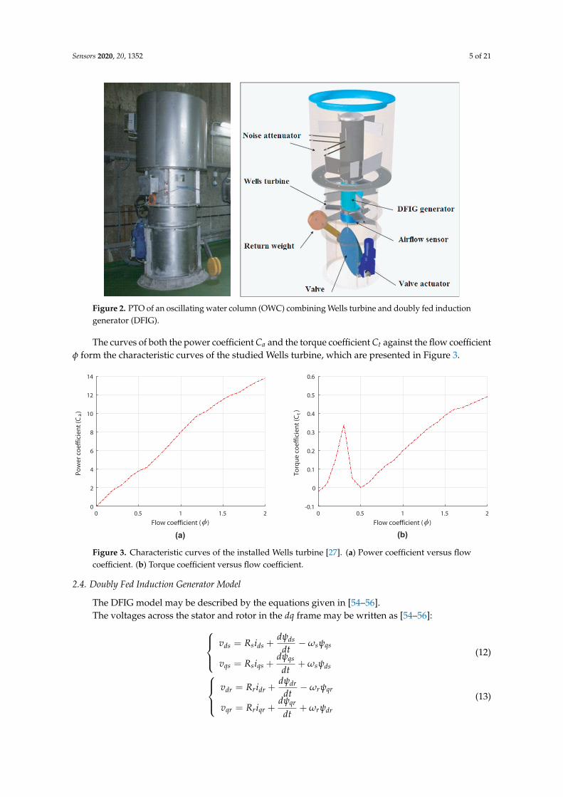
Figure 2. PTO of an oscillating water column (OWC) combining Wells turbine and doubly fed inductiongenerator (DFIG).

The curves of both the power coefficient Ca and the torque coefficient Ct against the flow coefficientφ form the characteristic curves of the studied Wells turbine, which are presented in Figure 3.

Flow coefficient ( )

0 0.5 1 1.5 2

Po

we

r co

eff

icie

nt

(Ca

)

0

2

4

6

8

10

12

14

Flow coefficient ( )

0 0.5 1 1.5 2

To

rqu

e c

oe

ffic

ien

t (C

t)

-0.1

0

0.1

0.2

0.3

0.4

0.5

0.6

ϕϕ

(a) (b)

Figure 3. Characteristic curves of the installed Wells turbine [27]. (a) Power coefficient versus flowcoefficient. (b) Torque coefficient versus flow coefficient.

2.4. Doubly Fed Induction Generator Model

The DFIG model may be described by the equations given in [54–56].The voltages across the stator and rotor in the dq frame may be written as [54–56]:

vds = Rsids +dψds

dt−ωsψqs

vqs = Rsiqs +dψqs

dt+ ωsψds

(12)

vdr = Rridr +

dψdrdt−ωrψqr

vqr = Rriqr +dψqr

dt+ ωrψdr

(13)

Sensors 2020, 20, 1352 6 of 21

where Rs and Rr are the stator and the rotor resistances, ωs and ωr are the stator and the rotor angularvelocities, ids and iqs are the d-q stator currents, idr and iqr are the d-q rotor currents.

The flux linkage in the stator and the rotor may be written as:ψds = Lssids + Lmidrψqs = Lssiqs + Lmiqr

(14)ψdr = Lrridr + Lmidsψqr = Lrriqr + Lmiqs

(15)

where Lss and Lrr are the stator and the rotor inductances, and Lm is the magnetizing inductance.The generated electromagnetic torque may be expressed as:

Te =32

p(ψdsiqs − ψqsids

)(16)

where p is the pair pole number.The mechanical interaction between the turbine and the generator can be defined as:

Jp

dωr

dt= Te − Tt (17)

where J is the inertia of the system.

3. Problem Statement

The OWC understudy consists of a Wells turbine coupled to DFIG, however, as already mentioned,the aerodynamics of the turbine gets affected by the stalling phenomenon when reaching a criticalflow rate value. In fact, this behavior occurs when the airflow velocity vx rises quickly, but the slowdynamics of the DFIG prevent the rotational speed ωr from changing as quick. The stalling effectcan be deduced from Figure 3b, which indicates that when the flow coefficient φ surpasses a certainthreshold (which is 0.3 for this turbine), the torque coefficient Ct drops drastically.

The flow coefficient φ described by Equation (9) depends on the airflow speed vx.However, as described by Equation (5), vx depends on the wave amplitude and period. In fact,the higher the wave amplitude and the shorter the period are, the stronger the wave power and theairflow speed are, as explained by Figure 4.

0

Wave periode (s)

5

10

150

0.5

1

Wave amplitude (m)

1.5

100

0

300

200

2

Air

flow

sp

eed

(m

/s)

Figure 4. Airflow speed variation for different wave amplitudes and periods.

The stalling effect is shown by studying the uncontrolled OWC plant in two sea conditions; thefirst one is a wave with a 10 s period and a wave amplitude of 0.9 m starting from 0 s to 22.5 s and the

Sensors 2020, 20, 1352 7 of 21

second one is a wave with a 10 s period and a wave amplitude of 1.2 m from 22.5 to 50 s. Figure 5 showsthat the first sea condition provides a flow coefficient lower than the threshold value 0.3, whereas,with the second sea condition, it exceeds the threshold value.

Time (s)

0 5 10 15 20 25 30 35 40 45 50

Flo

w c

oe

ffic

ien

t

0

0.1

0.2

0.3

0.4

0.5

0.6

A=1.20m

A=0.90m

Figure 5. Flow coefficient vs. time for two wave amplitudes [27].

Accordingly, the obtained torques shown in Figure 6 indicate no stalling for the first sea conditionand a drastic decrease at the crest in the second sea condition by the stalling effect. This will decreasethe produced torque in terms of the average value.

Time (s)

0 5 10 15 20 25 30 35 40 45 50

Tu

rbin

e t

orq

ue

(N

.m)

0

20

40

60

80

100

120

140

160

No Stalling Stalling behaviour

Figure 6. Turbine torques vs. time for two sea conditions [27].

4. Control Statement

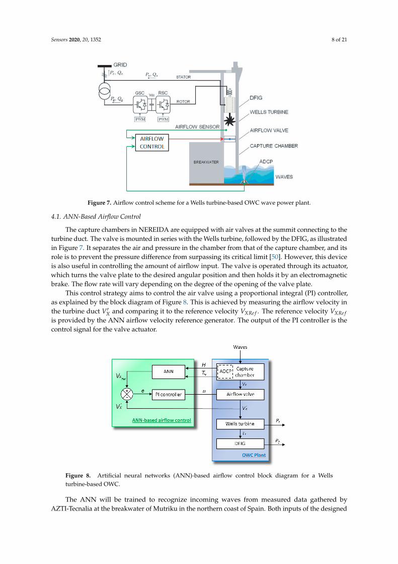
The stalling phenomenon of the Wells turbine may be avoided by continuously adjusting the flowcoefficient [48,49]. By referring to Equation (7), the flow coefficient depends on the airflow speed inthe turbine duct. Hence, regulating the airflow velocity vx will help avoid the stalling effect. In thissense, an ANN-based airflow control scheme has been proposed to control the air valve situated insidethe capture chamber of the OWC system in order to regulate the airflow speed vx, thus keeping theflow coefficient φ under the threshold value. The ANN will be trained to recognize incoming wavesfrom measured data by the acoustic doppler current profiler (ADCP). The scheme of the proposedANN-airflow control strategy is presented in Figure 7.

Sensors 2020, 20, 1352 8 of 21

Figure 7. Airflow control scheme for a Wells turbine-based OWC wave power plant.

4.1. ANN-Based Airflow Control

The capture chambers in NEREIDA are equipped with air valves at the summit connecting to theturbine duct. The valve is mounted in series with the Wells turbine, followed by the DFIG, as illustratedin Figure 7. It separates the air and pressure in the chamber from that of the capture chamber, and itsrole is to prevent the pressure difference from surpassing its critical limit [50]. However, this deviceis also useful in controlling the amount of airflow input. The valve is operated through its actuator,which turns the valve plate to the desired angular position and then holds it by an electromagneticbrake. The flow rate will vary depending on the degree of the opening of the valve plate.

This control strategy aims to control the air valve using a proportional integral (PI) controller,as explained by the block diagram of Figure 8. This is achieved by measuring the airflow velocity inthe turbine duct V′X and comparing it to the reference velocity VXRe f . The reference velocity VXRe fis provided by the ANN airflow velocity reference generator. The output of the PI controller is thecontrol signal for the valve actuator.

Figure 8. Artificial neural networks (ANN)-based airflow control block diagram for a Wellsturbine-based OWC.

The ANN will be trained to recognize incoming waves from measured data gathered byAZTI-Tecnalia at the breakwater of Mutriku in the northern coast of Spain. Both inputs of the designed

Sensors 2020, 20, 1352 9 of 21

ANN are obtained from the acoustic doppler current profiler (ADCP) installed at Mutriku (shown inFigure 9). The considered data are from 12 May 2014, where measurements of the first 20 min wererecorded every 2 h. The installed ADCP is of Workhorse 600 kHz from Teledyne RDI with a samplingperiod of 0.5 s.

Figure 9. Acoustic doppler current profiler in Mutriku.

ADCPs are hydro-acoustic devices used to measure water current velocities. This technology usesthe Doppler effect of sound waves scattered back from particles. It is able to send and receive soundsignals thanks to piezoelectric transducers. The time it takes sound waves to travel allows estimatingthe distance. The frequency shift of the echo is proportional to the water velocity within the acousticpath. Three-dimensional velocity measurements require a minimum of three beams [57,58].

In the last few years, more functionality has been added to ADCPs to include wave and turbulencemeasurements. The ADCP device specific to wave characteristic measurements is known as the acousticwave and current (AWAC) profiler, which allows the measurement of surface wave height and itsdirection [59,60]. The one installed in Mutriku is mounted upwards down at the seafloor. The AWACdevice has four transducers that transmit four beams; one transducer in the middle point vertically up,and three transducers symmetrically positioned at 120 degrees from each other and surrounding thecenter one, and they are angled off the vertical by 25 degrees [61,62].

4.2. ANN Airflow Velocity Reference Generator

The trained ANN has to generate reference airflow velocity that does not provoke the stallingbehavior of the Wells turbine, this means that when the wave power is low, the total airflow is admittedby the valve, but when the waves are strong enough to generate high airflow speed, the valve shouldblock the incoming airflow to reduce its speed. In this sense, numerous simulations were carriedout to record the acceptable waves and distinguish the strong waves that provoke the stalling effect.Hence, input–output data sets have been assembled to train the network into generating the desiredoutput. The desired airflow reference as a function of the wave amplitude and period is shown inFigure 10.

The ANN developed is a feed-forward network controller that consists of an input layer of twoneurons; one for the wave amplitude, and the other one for the wave period, and an output layerwith one neuron representing the desired airflow speed reference. Determining the number of hiddenlayers/neurons in such a complex system is an intricate task; therefore, the trial-and-error rule based onthe forward approach procedure has been used [63]. The method begins with an undersized number ofhidden layers/neurons and then increases them. At every time, the new network structure is trainedand tested. This process is repeated until the train and test results are improved. By statistical analysis,the best structure is selected by choosing the best mean squared error (MSE).

Sensors 2020, 20, 1352 10 of 21

02

46

Wave period (s)

810

1214

1600.25

0.50Wave amplitude (m)

0.751

1.251.50

1.75

40

30

10

0

20

2

Air

flow

sp

eed

(m

/s)

Figure 10. Desired airflow speed for different wave amplitudes and periods.

ANNs consist of neurons in the input, output, and hidden layers, which are connected withweighted signals (wij). The neurons consist of a bias bj, a sum function Sj coupled to an activationfunction ϕj. The sum function may be defined as:

Sj =N

∑j=1

(wjiyi) + bj (18)

where Sj is the sum from the jth neuron from the current layer, bj is the bias, N is the total number ofneurons, wji is the weight of the signal connecting the jth neuron from the current layer with the ith

neuron from the previous layer, and yi is the input signal from the neuron of the previous layer.The activation function of neurons in the input layer is clamped by the input vector; however,

the activation function of the rest of the neurons in the network can be chosen as:

yj = ϕj(Sj) =

Sj (Linear)

11+e−Sj

(Sigmoid)

eSj−e−Sj

eSj+e−Sj(Hyperbolic tangent)

(19)

To train the ANN, the Levenberg–Marquardt (LM) algorithm has been considered as a learningmethod [64]. This algorithm is a variant of Newton’s method, which was designed to minimizefunctions that are sums of squares of nonlinear functions [65]. The algorithm aims to update thenetwork weights in order to minimize the performance index by [66]:

∆X =[∇2F(X)

]−1∇F(X) (20)

where F(X) is the performance index, ∇F(X) is the gradient, and ∇2F(X) the Hessian matrix.Knowing that the performance index is defined as:

F(X) =N

∑i=1

E2i (X) = ET(X).E(X) (21)

where E(X) is the error between the ANN’s output and the target output.The gradient of the performance index may be written as:

∇F(X) = 2JT(X).E(X) (22)

Sensors 2020, 20, 1352 11 of 21

where J(X) is the Jacobian matrix defined as [67]:

J(X) =

∂E1(X)

∂X1

∂E1(X)∂X2

. . . ∂E1(X)∂Xn

∂E2(X)∂X1

∂E2(X)∂X2

. . . ∂E2(X)∂Xn

......

. . ....

∂EN(X)∂X1

∂EN(X)∂X2

· · · ∂EN(X)∂Xn

(23)

where n is the number of training patterns.Hence, the Hessian matrix may be expressed as:

∇2F(X) = 2JT(X).J(X) + 2N

∑i=1

Ei(X).∇2Ei(X) (24)

5. Results and Discussion

This section presents the simulations carried out to evaluate the performance of theproposed ANN-based airflow control. To evaluate the performance of the proposed controlmethodology, the OWC wave power plant has been implemented by a complete wave-to-wiremodel on Matlab/Simulink, and a comparison between the uncontrolled and controlled cases hasbeen performed.

To implement the OWC model, we considered the parameters obtained from real measurementsat the NEREIDA wave power plant. These parameters were provided by the Basque Energy Agency(EVE) and are detailed in Table 1.

Table 1. Plant parameters from the NEREIDA wave power plant at Mutriku.

Capture Chamber Wells Turbine DFIG Generator

wc = 4.5 m n = 5 Rs = 0.5968 Ω Prated = 18.45 kWlc = 4.3 m b = 0.21 m Rr = 0.6258 Ω Vsrated = 400 V

ρa = 1.19 kg/m3 l = 0.165 m Lss = 0.0003495 H frated = 50 Hzρw = 1029 kg/m3 r = 0.375 m Lrr = 0.324 H p = 2

a = 0.4417 m2 Lm = 0.324 H

5.1. ANN Training Performance

Using the trial-and-error rule based on the forward approach procedure, several structures withdifferent hidden layers and neurons were tested with our problem in order to obtain the best MSE.The activation function used for the neurons in the hidden layer is the hyperbolic tangent, whereas inthe output layer, the linear activation function. During the simulation tests, the comparative studytakes into account the number of epochs and the least MSE. The training process was performed oncomputers with a 3.2 GHz Intel Core i7-8700 Six-Core processor and Integrated Intel UHD Graphics630. Table 2 shows the results obtained of training different networks with different structures appliedto the problem of wave characteristics recognition.

Sensors 2020, 20, 1352 12 of 21

Table 2. Training performance of different structures using the Levenberg–Marquardt algorithm.

Network Structure Epochs MSE Network Structure Epochs MSE

11 1.1196 237 1.0463 × 10−3

2 × 2 × 1 20 8.0244 × 10−1 2 × 2 × 2 × 1 453 9.8214 × 10−4

56 7.3278 × 10−1 619 8.1576 × 10−4

98 3.8778 × 10−1 862 8.6248 × 10−4

68 1.5626 × 10−1 202 8.5032 × 10−4

2 × 4 × 1 122 9.0921 × 10−2 2 × 4 × 2 × 1 534 7.9368 × 10−4

566 6.6619 × 10−2 811 8.2294 × 10−4

698 4.2215 × 10−2 1000 7.6146 × 10−4

188 4.2318 × 10−2 115 9.0408 × 10−4

2 × 8 × 1 528 5.4049 × 10−3 2 × 2 × 4 × 1 482 7.7924 × 10−4

706 7.6852 × 10−3 (ANN1) 726 8.1396 × 10−4

1000 2.3425 × 10−3 1000 6.4947 × 10−4

307 1.7154 × 10−3 98 8.3164 × 10−4

2 × 16 × 1 423 1.3220 × 10−3 2 × 4 × 4 × 1 137 6.9595 × 10−5

775 7.3013 × 10−4 (ANN2) 546 8.0274 × 10−4

1000 8.8384 × 10−4 934 7.0812 × 10−4

From the results of Table 2, we can deduce that the results obtained using a single hidden layernetworks, known as Vanilla neural networks, performs poorly due to the nonlinearity and complexityof the problem. On the other hand, network structures with more than one hidden layer, known asdeep neural networks, offer better performance. Therefore, further analysis was carried out on thecurves of the training performance of the deep neural network structures, with the best results markedas ANN1 (2 × 2 × 4 × 1) and ANN2 (2 × 4 × 4 × 1) in order to select the adequate structure.

The evolution of the training process of ANN1 (2 × 2 × 4 × 1) is depicted in Figure 11, and theone of ANN2 (2 × 4 × 4 × 1) is depicted in Figure 12. From these figures, it can be noticed that in thecase of ANN1, the training process took more epochs to converge to the minimum MSE of 6.4947 ×10−4; however, with ANN2, it converged to a smaller MSE of 6.9595 × 10−5 in fewer epochs at 137.

1000 Epochs

0 100 200 300 400 500 600 700 800 900 1000

Me

an

Sq

ua

red

Err

or

(m

se)

10-4

10-2

100

102

Best Validation Performance is 0.00064947 at epoch 1000

Train

Validation

Test

Best

Figure 11. Training performance for a network of 2 × 2 × 4 × 1 (ANN1).

Sensors 2020, 20, 1352 13 of 21

1000 Epochs

0 100 200 300 400 500 600 700 800 900 1000

Me

an

Sq

ua

red

Err

or

(m

se)

10-4

10-2

100

102

Best Validation Performance is 6.9595e-05 at epoch 137

Train

Validation

Test

Best

Figure 12. Training performance for a network of 2 × 4 × 4 × 1 (ANN2).

Finally, the topology of ANN2 has been selected as the ANN airflow velocity reference generatorto be implemented in the proposed airflow control scheme to provide the desired airflow speed.

5.2. Control Assessment with Regular Waves

To evaluate the power generation enhancement of the proposed ANN-based airflow controlscheme, a study case considering two representative sea states from the site of Mutriku are selectedfrom the wave spectrum of the location illustrated in Figure 13.

Figure 13. Representative spectral analysis of the waves at the site Mutriku on 12 May 2014 [27].

The waves are characterized by a water depth h = 5 m and a wave period Tw = 10 s. The firstwave amplitude is A = 0.9 m from 0 s to 22.5 s, and the second wave amplitude is A = 1.2 m from22.5 s to 50 s, as shown in Figure 14.

Time (s)

0 5 10 15 20 25 30 35 40 45 50

Wa

ve

ele

va

tio

n (

m)

-2

-1

0

1

2

A=0.90m

A=1.20m

Figure 14. Considered wave input to the implemented OWC model.

Sensors 2020, 20, 1352 14 of 21

Figure 15 shows the airflow speed for both waves in the uncontrolled and controlled cases.The curves show that for the first sea condition, the airflow velocity is in the acceptable range,whereas for the second wave, the neural network recognized the wave as one that will provoke astalling behavior in the OWC; therefore, the control has been activated and the speed has been reducedby the air valve.

Time (s)

0 5 10 15 20 25 30 35 40 45 50

Air

flo

w v

elo

city

(m

/s)

0

10

20

30

40

50

Uncontrolled

ANN airflow control

Figure 15. Airflow speed for uncontrolled case and ANN-based airflow control.

The flow coefficients are presented in Figure 16 and show that, indeed, the flow coefficient of thefirst wave did not exceed the threshold value of 0.3 in the uncontrolled case, which required no actionin the controlled case. However, in the case of the second wave, the flow coefficient did exceed thethreshold value; hence, the control managed to successfully adjust it.

Time (s)

0 5 10 15 20 25 30 35 40 45 50

Flo

w c

oe

ffic

ien

t

0

0.1

0.2

0.3

0.4

0.5

0.6

Uncontrolled

ANN airflow control

Figure 16. Flow coefficients for uncontrolled case and ANN-based airflow control.

The resulting produced torques are shown in Figure 17, where it is clearly observed that with thesecond wave, the torque in the uncontrolled case has a drastic decrease at every crest, which reducesthe torque in terms of average value. However, using the ANN-airflow control, the torque has beenmaintained at the maximum value, thus maintaining a higher average value.

Time (s)

0 5 10 15 20 25 30 35 40 45 50

Tu

rbin

e t

orq

ue

(N

.m)

0

20

40

60

80

100

120

140

160

Uncontrolled

ANN airflow control

Figure 17. Turbine torque for uncontrolled case and ANN-based airflow control.

Sensors 2020, 20, 1352 15 of 21

Eventually, the generated power avoided the power drop at the peak of the second wave, as shownin Figure 18. Therefore, the generated power is higher in terms of the average value with the use of theANN-based airflow control.

Time (s)

0 5 10 15 20 25 30 35 40 45 50

Ge

ne

rate

d p

ow

er

(W)

× 104

-4

-3

-2

-1

0

1

2

Uncontrolled

ANN airflow controlStalling

Stalling avoided

Figure 18. Generated power for uncontrolled case and ANN-based airflow control.

5.3. Control Assessment with Real Measured Wave Data

In this comparative study, we considered real surface elevation measurements of waves in Mutrikuobtained by the Acoustic Doppler Current Profiler on 12 May 2014, at 00:00:00, as shown in Figure 19.This measured input will help test the proposed control with other wave amplitudes and periods.

-1,000

-0,500

0,000

0,500

1,000

1,500

Wave Height (m)

Figure 19. Measured wave input to the implemented OWC model.

The curves of the airflow speed in Figure 20 showed fast airflow at the peak of the waves,namely at 5, 8, 38, and 48 s. Effectively, the ANN controller activated the airflow control, and the speedhas been reduced by the air valve.

Time (s)

0 5 10 15 20 25 30 35 40 45 50

Air

flo

w v

elo

city

(m

/s)

0

20

40

60

80

100Uncontrolled

ANN airflow control

Figure 20. Airflow speed for uncontrolled case and ANN-based airflow control.

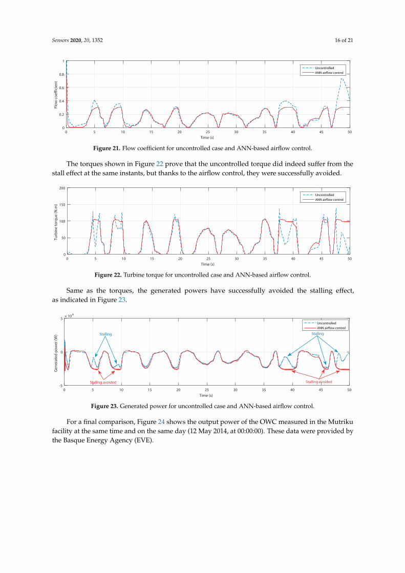
Confirming with the curves of the airflow speed, the flow coefficients, shown in Figure 21,have indeed exceeded the threshold value at the indicated instances when uncontrolled. The controlledOWC, however, shows a regulation of the coefficient at the threshold value 0.3.

Sensors 2020, 20, 1352 16 of 21

Time (s)

0 5 10 15 20 25 30 35 40 45 50

Flo

w c

oe

ffic

ien

t

0

0.2

0.4

0.6

0.8

1

Uncontrolled

ANN airflow control

Figure 21. Flow coefficient for uncontrolled case and ANN-based airflow control.

The torques shown in Figure 22 prove that the uncontrolled torque did indeed suffer from thestall effect at the same instants, but thanks to the airflow control, they were successfully avoided.

Time (s)

0 5 10 15 20 25 30 35 40 45 50

Tu

rbin

e t

orq

ue

(N

.m)

0

50

100

150

200

Uncontrolled

ANN airflow control

Figure 22. Turbine torque for uncontrolled case and ANN-based airflow control.

Same as the torques, the generated powers have successfully avoided the stalling effect,as indicated in Figure 23.

Time (s)

0 5 10 15 20 25 30 35 40 45 50

Ge

ne

rate

d p

ow

er

(W)

× 104

-5

0

5Uncontrolled

ANN airflow control

Stalling

Stalling avoidedStalling avoided

Stalling

Figure 23. Generated power for uncontrolled case and ANN-based airflow control.

For a final comparison, Figure 24 shows the output power of the OWC measured in the Mutrikufacility at the same time and on the same day (12 May 2014, at 00:00:00). These data were provided bythe Basque Energy Agency (EVE).

Sensors 2020, 20, 1352 17 of 21

-50

-40

-30

-20

-10

0

10

20

30

40

50

Generated Power (kW)

Figure 24. Generated power measured at the NEREIDA wave power plant of Mutriku.

By taking into consideration the quality of the data series due to the large sampling period,one can see the same waveform in both the numerical power of Figures 23 and 24. However, at theinstants 5, 8, 18, 38, and 48 s, the controlled power is superior to the measured power.

6. Conclusions

In this article, the modeling and implementation of an OWC system using a Wells turbine coupledto a DFIG has been presented. The paper also proposes a novel ANN-based airflow control for theOWC to deal with the stalling behavior of the Wells turbine, which proves to limit the generated power.

The proposed ANN-airflow control uses a trained artificial neural network to recognize waveswith high airflow speed that may cause a stalling effect in the system. The data used to train the ANNwere gathered by an Acoustic Doppler Current Profiler. The ANN is then able to generate an adequateairflow speed reference. The reference is used in the airflow control scheme. To design the suitablenetwork structure for the problem, numerous simulations were performed using the trial-and-errorrule based on the forward approach procedure. The best topology has been selected by consideringthe best performance index MSE, the number of epochs, and the least complicated structure.

The results of the training process showed that the best MSE is obtained with deep neuralnetworks. The considered ANN topology was able to converge in an acceptable number of epochs.Using the trained network in the airflow scheme, the airflow strategy has been able to detect strongwaves and avoid the stalling behavior. The results prove the effectiveness of the control with differentsea states. Also, a comparative study using real surface elevation measurements of waves in Mutrikushowed good avoidance of the stalling phenomenon even compared to the measured power output ofthe NEREIDA plant in Mutriku.

Author Contributions: All authors contributed to the modeling and implementation of the OWC plant. Allauthors conceived, developed, and implemented the control techniques. All authors analyzed and validated theresults. All authors contributed to writing—review and editing of the manuscript. All authors have read andagreed to the published version of the manuscript.

Funding: This work was supported in part by the Basque Government, through project IT1207-19 and by theMCIU/MINECO through RTI2018-094902-B-C21/RTI2018-094902-B-C22 (MCIU/AEI/FEDER, UE).

Acknowledgments: The authors would like to thank the editors and reviewers for the constructive commentsthat have helped to improve the initial version of the manuscript.

Conflicts of Interest: The authors declare no conflict of interest.

Sensors 2020, 20, 1352 18 of 21

Nomenclature

The following symbols are used in this manuscript:

λ, A, H Wavelength, amplitude, and height (m)h, z Sea depth and wave surface elevation (m)Tw, ω Wave period (s) and wave frequency (rad/s)g Acceleration gravity (m/s2)P, dP Capture chamber pressure and Pressure drop (Pa)wc, lc Capture chamber inner width and length (m)V, Q Capture chamber volume (m3) and flow rate (m3/s)ρ, vx Atmospheric density (kg/m3) and airflow speed (m/s)l, b, D Blade chord length, blade span and turbine diameter (m)n, p, k, K Blade number, pole number, wave number and turbine constantTe, Tt Electromagnetic and turbine torques (N.m)J Turbo-generator inertia (kg.m2)Ct, Ca, φ Torque, power and flow coefficientsRs, Rr Stator and rotor resistances (Ω)Ls, Lr Stator and rotor inductances (H)is, ir Stator and rotor currents (A)ψs, ψr Stator and rotor flux (Wb)ωs, ωr Stator and rotor rotational speed (rad/s)Sj, ϕj, bj Sum function, activation function, bias and output of the jth neuronyi, yj output of ith neuron from previous layer and output of the jth neuron from current layerwji Weight of signal connecting ith neuron from previous layer to jth neuron of current layer

References

1. Huckerby, J.; Jeffrey, H.; Jay, B.; Executive, O. An International Vision for Ocean Energy; Ocean Energy Systems:Lisbon, Portugal, 2011.

2. Brito, A.; Villate, J.L. Annual Report 2014: Implementing Agreement on Ocean Energy Systems; Ocean EnergySystems: Lisbon, Portugal, 2015.

3. Lehmann, M.; Karimpour, F.; Goudey, C.A.; Jacobson, P.T.; Alam, M.R. Ocean wave energy in the UnitedStates: Current status and future perspectives. Renew. Sustain. Energy Rev. 2017, 74, 1300–1313. [CrossRef]

4. Alamir, M.; Fiacchini, M.; Chabane, S.B.; Bacha, S.; Kovaltchouk, T. Active power control under Grid Codeconstraints for a tidal farm. In Proceedings of the 2016 Eleventh International Conference on EcologicalVehicles and Renewable Energies (EVER), New York, NY, USA, 6–8 April 2016; pp. 1–7.

5. Magagna, D.; Uihlein, A. 2014 JRC Ocean Energy Status Report; European Commission: Luxembourg, 2015.6. Rusu, L.; Onea, F. Assessment of the performances of various wave energy converters along the European

continental coasts. Energy 2015, 82, 889–904. [CrossRef]7. Heath, T.V. A review of oscillating water columns. Philos. Trans. R. Soc. A Math. Phys. Eng. Sci. 2012, 370,

235–245. [CrossRef] [PubMed]8. Lagoun, M.S.; Benalia, A.; Benbouzid, M.H. Ocean wave converters: State of the art and current status.

In Proceedings of the 2010 IEEE International Energy Conference, Manama, Bahrain, 18–22 December 2010;pp. 636–641.

9. Yemm, R.; Pizer, D.; Retzler, C.; Henderson, R. Pelamis: Experience from concept to connection. Philos. Trans.R. Soc. A Math. Phys. Eng. Sci. 2012, 370, 365–380. [CrossRef]

10. Kofoed, J.P.; Frigaard, P.; Friis-Madsen, E.; Sørensen, H.C. Prototype testing of the wave energy converterwave dragon. Renew. Energy 2006, 31, 181–189. [CrossRef]

11. Westwood, A. SeaGen installation moves forward. Renew. Energy Focus 2008, 9, 26–27. [CrossRef]12. Calcagno, G.; Salvatore, F.; Greco, L.; Moroso, A.; Eriksson, H. Experimental and numerical investigation

of an innovative technology for marine current exploitation: The Kobold turbine. In Proceedingsof the Sixteenth International Offshore and Polar Engineering Conference, San Francisco, CA, USA,28 May–2 June 2006; pp. 323–330.

Sensors 2020, 20, 1352 19 of 21

13. Kinsey, T.; Dumas, G.; Lalande, G.; Ruel, J.; Mehut, A.; Viarouge, P.; Lemay, J.; Jean, Y. Prototype testing ofa hydrokinetic turbine based on oscillating hydrofoils. Renew. Energy 2011, 36, 1710–1718. [CrossRef]

14. Stopa, J.E.; Cheung, K.F.; Chen, Y.L. Assessment of wave energy resources in Hawaii. Renew. Energy 2011, 36,554–567. [CrossRef]

15. Liberti, L.; Carillo, A.; Sannino, G. Wave energy resource assessment in the Mediterranean, the Italianperspective. Renew. Energy 2013, 50, 938–949. [CrossRef]

16. Kumar, V.S.; Anoop, T.R. Wave energy resource assessment for the Indian shelf seas. Renew. Energy 2015, 76,212–219. [CrossRef]

17. López, M.; Veigas, M.; Iglesias, G. On the wave energy resource of Peru. Energy Convers. Manag. 2015, 90,34–40. [CrossRef]

18. Drew, B.; Plummer, A.R.; Sahinkaya, M.N. A review of wave energy converter technology. Proc. Inst. Mech.Eng. A J. Power Energy 2009, 223, 887–902. [CrossRef]

19. Antonio, F.D.O. Wave energy utilization: A review of the technologies. Renew. Sustain. Energy Rev. 2010, 14,899–918.

20. Corsatea, T.D.; Magagna, D. Overview of European Innovation Activities in Marine Energy Technology; JRCScience and Policy Reports; European Commission: Brussels, Belgium, 2013.

21. European Commission. Report on the Blue Growth Strategy Towards More Sustainable Growth and Jobs inthe Blue Economy; European Commission: Brussels, Belgium, 2017; pp. 1–62. Available online: Https://ec.europa.eu/maritimeaffairs/policy/blue_growth_en (accessed on 28 February 2020).

22. Raghunathan, S. Performance of the Wells self-rectifying turbine. Aeronaut. J. 1985, 89, 369–379.23. Raghunathan, S. The wells air turbine for wave energy conversion. Prog. Aerospace Sci. 1995, 31, 335–386.

[CrossRef]24. Falcão, A.D.O.; Justino, P.A.P. OWC wave energy devices with air flow control. Ocean Eng. 1999, 26,

1275–1295. [CrossRef]25. Amundarain, M.; Alberdi, M.; Garrido, A.J.; Garrido, I. Modeling and simulation of wave energy generation

plants: Output power control. IEEE Trans. Ind. Electron. 2010, 58, 105–117. [CrossRef]26. Mishra, S.K.; Purwar, S.; Kishor, N. Air flow control of OWC wave power plants using FOPID controller.

In Proceedings of the 2015 IEEE Conference on Control Applications (CCA), Sydney, Australia, 19–22September 2016; pp. 1516–1521.

27. M’zoughi, F.; Garrido, I.; Bouallègue, S.; Ayadi, M.; Garrido, A.J. Intelligent Airflow Controls fora Stalling-Free Operation of an Oscillating Water Column-Based Wave Power Generation Plant. Electronics2019, 8, 70. [CrossRef]

28. Omidvar, O.; Elliott, D.L. Neural Systems for Control; Academic Press: Cambridge, MA, USA, 1997;ISBN 9780080537399.

29. Yilmaz, A.S.; Ozer, Z. Pitch angle control in wind turbines above the rated wind speed by multi-layerperceptron and radial basis function neural networks. Expert Syst. Appl. 2009, 36, 9767–9775. [CrossRef]

30. Alberdi, M.; Amundarain, M.; Garrido, A.; Garrido, I. Neural control for voltage dips ride-through ofoscillating water column-based wave energy converter equipped with doubly-fed induction generator.Renew. Energy 2012, 48, 16–26. [CrossRef]

31. Legowski, A.; Niezabitowski, M. An industrial robot singular trajectories planning based on graphs andneural networks. AIP Conf. Proc. 2016, 1738, 480057.

32. Bertachi, A.; Biagi, L.; Contreras, I.; Luo, N.; Vehí, J. Prediction of Blood Glucose Levels And NocturnalHypoglycemia Using Physiological Models and Artificial Neural Networks. In Proceedings of the KHD@IJCAI, Stockholm, Schweden, 13–19 July 2018; pp. 85–90.

33. Farooq, Z.; Zaman, T.; Khan, M.A.; Muyeen, S.M.; Ibeas, A. Artificial Neural Network Based AdaptiveControl of Single Phase Dual Active Bridge With Finite Time Disturbance Compensation. IEEE Access 2019,7, 112229–112239. [CrossRef]

34. Krzyszczak, J.; Baranowski, P.; Zubik, M.; Hoffmann, H. Temporal scale influence on multifractal propertiesof agro-meteorological time series. Agric. For. Meteorol. 2017, 239, 223–235. [CrossRef]

35. Castañeda-Miranda, A.; Icaza-Herrera, M.D.; Castaño, V.M. Meteorological Temperature and HumidityPrediction from Fourier-Statistical Analysis of Hourly Data. Adv. Meteorol. 2019, 2019, 1–13. [CrossRef]

36. Yang, Z.C. Hourly ambient air humidity fluctuation evaluation and forecasting based on the least-squaresFourier-model. Measurement 2019, 133, 112–123. [CrossRef]

Sensors 2020, 20, 1352 20 of 21

37. Stoyanov, D.B.; Nixon, J.D. Alternative operational strategies for wind turbines in cold climates. Renew.Energy 2020, 145, 2694–2706. [CrossRef]

38. Castañeda-Miranda, A.; Castaño, V.M. Smart frost control in greenhouses by neural networks models.Comput. Electron. Agric. 2017, 137, 102–114. [CrossRef]

39. Li, C.; Zhou, D.; Wang, H.; Lu, Y.; Li, D. Techno-economic performance study of stand-alonewind/diesel/battery hybrid system with different battery technologies in the cold region of China. Energy2020, 192, 116702. [CrossRef]

40. Konispoliatis, D.N.; Mavrakos, S.A. Natural frequencies of vertical cylindrical oscillating water columndevices. Appl. Ocean Res. 2019, 91, 101894. [CrossRef]

41. Zheng, S.; Zhu, G.; Simmonds, D.; Greaves, D.; Iglesias, G. Wave power extraction from a tubular structureintegrated oscillating water column. Renew. Energy 2020, 150, 342–355. [CrossRef]

42. Singh, U.; Abdussamie, N.; Hore, J. Hydrodynamic performance of a floating offshore OWC wave energyconverter: An experimental study. Renew. Sustain. Energy Rev. 2020, 117, 109501. [CrossRef]

43. Sobey, R.; Goodwin, P.; Thieke, R.; Westberg, R.J., Jr. Application of Stokes, Cnoidal, and Fourier wavetheories. J. Waterway Port Coast. Ocean Eng. 1987, 113, 565–587. [CrossRef]

44. Le Roux, J.P. An extension of the Airy theory for linear waves into shallow water. Coast. Eng. 2008, 55,295–301. [CrossRef]

45. Garrido, A.J.; Otaola, E.; Garrido, I.; Lekube, J.; Maseda, F.J.; Liria, P.; Mader, J. Mathematical Modeling ofOscillating Water Columns Wave-Structure Interaction in Ocean Energy Plants. Math. Prob. Eng. 2015, 2015,1–11. [CrossRef]

46. Sarmento, A.J.N.A.; de Falcão, A.F.O. Wave generation by an oscillating surface-pressure and its applicationin wave-energy extraction. J. Fluid Mech. 1985, 150, 467–485. [CrossRef]

47. Falcão, A.F.O.; Rodrigues, R.J.A. Stochastic modelling of OWC wave power plant performance. Appl. OceanRes. 2002, 24, 59–71. [CrossRef]

48. M’zoughi, F.; Bouallègue, S.; Garrido, A.J.; Garrido, I.; Ayadi, M. Stalling-free Control Strategies forOscillating-Water-Column-based Wave Power Generation Plants. IEEE Trans. Energy Convers. 2018, 33,209–222. [CrossRef]

49. M’zoughi, F.; Bouallègue, S.; Garrido, A.J.; Garrido, I.; Ayadi, M. Water Cycle Algorithm-based AirflowControl for an Oscillating Water Column-based Wave Generation Power Plant. Proc. Inst. Mech. Eng. Part I J.Syst. Control Eng. 2020, 234, 118–133. [CrossRef]

50. M’zoughi, F.; Bouallègue, S.; Garrido, A. J.; Garrido, I.; Ayadi, M. Fuzzy gain scheduled PI-based airflowcontrol of an oscillating water column in wave power generation plants. IEEE J. Ocean. Eng. 2019, 44,1058–1076. [CrossRef]

51. Falcão, A.F.O.; Gato, L.M.C. Air Turbines. In Comprehensive Renewable Energy; Sayigh, A., Ed.; 8: OceanEnergy; Elsevier: Oxford, UK, 2012; pp. 111–149.

52. López, I.; Andreu, J.; Ceballos, S.; de Alegría , I.M.; Kortabarria, I. Review of wave energy technologies andthe necessary power-equipment. Renew. Sustain. Energy Rev. 2013, 27, 413–434. [CrossRef]

53. Setoguchi, T.; Takao, M. Current status of self rectifying air turbines for wave energy conversion. EnergyConvers. Manag. 2006, 47, 2382–2396. [CrossRef]

54. Muller, S.; Diecke, M.; De Donker, R.W. Doubly fed induction generator systems for wind turbines. IEEE Ind.Appl. Mag. 2002, 8, 26–33. [CrossRef]

55. Ledesma, P.; Usaola, J. Doubly fed induction generator model for transient stability analysis. IEEE Trans.Energy Convers. 2005, 20, 388–397. [CrossRef]

56. M’zoughi, F.; Garrido, A.J.; Garrido, I.; Bouallègue, S.; Ayadi, M. Sliding Mode Rotational Speed Control ofan Oscillating Water Column-based Wave Generation Power Plants. In Proceedings of the 2018 InternationalSymposium on Power Electronics, Electrical Drives, Automation and Motion (SPEEDAM), Amalfi, Italy,20–22 Jun 2018; pp. 1263–1270.

57. Simpson, M.R. Discharge Measurements Using a Broad-Band Acoustic Doppler Current Profiler; US Departmentof the Interior, US Geological Survey: Reston, CA, USA, 2001.

58. Brumley, B.H.; Cabrera, R.G.; Deines, K.L.; Terray, E.A. Performance of a broad-band acoustic Dopplercurrent profiler. IEEE J. Ocean. Eng. 1991, 16, 402–407. [CrossRef]

59. Pedersen, T.; Nylund, S.; Dolle, A. Wave height measurements using acoustic surface tracking. In Proceedingsof the OCEANS’02 MTS/IEEE, Mississippi, MN, USA, 29–31 October 2002; Volume 3, pp. 1747–1754.

Sensors 2020, 20, 1352 21 of 21

60. Pedersen, T.; Siegel, E.; Wood, J. Directional wave measurements from a subsurface buoy with an acousticwave and current profiler (AWAC). In Proceedings of the OCEANS 2007, Vancouver, BC, Canada,29 September–4 October 2007; pp. 1–10.

61. Lohrmann, A.; Pedersen, T.K.; Nortek, A.S. System and Method for Determining Directional andNon-Directional Fluid Wave and Current Measurements. U.S. Patent 7,352,651, 1 April 2008.

62. Work, P.A. Nearshore directional wave measurements by surface-following buoy and acoustic Dopplercurrent profiler. Ocean Eng. 2008, 35, 727–737. [CrossRef]

63. Sheela, K.G.; Deepa, S.N. Review on methods to fix number of hidden neurons in neural networks.Math. Probl. Eng. 2013, doi:10.1155/2013/425740. [CrossRef]

64. Hagan, M.T.; Menhaj, M.B. Training feedforward networks with the Marquardt algorithm. IEEE Trans.Neural Netw. 1994, 5, 989–993. [CrossRef]

65. Wilamowski, B.M.; Yu, H. Improved computation for Levenberg–Marquardt training. IEEE Trans. NeuralNetw. 2010, 21, 930–937. [CrossRef]

66. Suratgar, A.A.; Tavakoli, M.B.; Hoseinabadi, A. Modified Levenberg–Marquardt method for neural networkstraining. Int. J. Comput. Inf. Eng. 2010, 6, 46–48.

67. Ampazis, N.; Perantonis, S.J. Levenberg–Marquardt algorithm with adaptive momentum for the efficienttraining of feedforward networks. In Proceedings of the IEEE-INNS-ENNS International Joint Conferenceon Neural Networks, Como, Italy, 24–27 July 2000; pp. 126–131.

c© 2020 by the authors. Licensee MDPI, Basel, Switzerland. This article is an open accessarticle distributed under the terms and conditions of the Creative Commons Attribution(CC BY) license (http://creativecommons.org/licenses/by/4.0/).