hydrodynamic analysis of oscillating water column wave ... · be hinged motions (e.g. pelamis...
TRANSCRIPT
General rights Copyright and moral rights for the publications made accessible in the public portal are retained by the authors and/or other copyright owners and it is a condition of accessing publications that users recognise and abide by the legal requirements associated with these rights.
Users may download and print one copy of any publication from the public portal for the purpose of private study or research.
You may not further distribute the material or use it for any profit-making activity or commercial gain
You may freely distribute the URL identifying the publication in the public portal If you believe that this document breaches copyright please contact us providing details, and we will remove access to the work immediately and investigate your claim.
Downloaded from orbit.dtu.dk on: Mar 11, 2020
Hydrodynamic analysis of oscillating water column wave energy devices
Bingham, Harry B.; Ducasse, Damien; Nielsen, Kim; Read, Robert
Published in:Journal of Ocean Engineering and Marine Energy
Link to article, DOI:10.1007/s40722-015-0032-4
Publication date:2015
Document VersionPublisher's PDF, also known as Version of record
Link back to DTU Orbit
Citation (APA):Bingham, H. B., Ducasse, D., Nielsen, K., & Read, R. (2015). Hydrodynamic analysis of oscillating water columnwave energy devices. Journal of Ocean Engineering and Marine Energy, 1(4), 405-419.https://doi.org/10.1007/s40722-015-0032-4

J. Ocean Eng. Mar. EnergyDOI 10.1007/s40722-015-0032-4
RESEARCH ARTICLE
Hydrodynamic analysis of oscillating water column wave energydevices
Harry B. Bingham1 · Damien Ducasse3 · Kim Nielsen2 · Robert Read1
Received: 20 January 2015 / Accepted: 15 June 2015© Springer International Publishing AG 2015
Abstract A 40-chamber I-Beam attenuator-type, oscil-lating water column, wave energy converter is analyzednumerically based on linearized potential flow theory, andexperimentally via model test experiments. The high-orderpanel method WAMIT by Newman and Lee (WAMIT; aradiation–diffraction panel program for wave-body interac-tions, 2014, http://www.wamit.com) is used for the basicwave-structure interaction analysis. The damping appliedto each chamber by the power take off is modeled in theexperiment by forcing the air through a hole with an areaof about 1% of the chamber water surface area. In thenumerical model, this damping is modeled by an equiva-lent linearized damping coefficient which extracts the sameamount of energy over one cycle as the experimentallymeasured quadratic damping coefficient. The pressure ineach chamber in regular waves of three different height-to-length ratios is measured in the experiments and comparedto calculations. The model is considered in both fixed andfreely floating, slack-moored conditions. Comparisons arealso made to experimental measurements on a single fixed
B Harry B. [email protected]
Damien [email protected]
Robert [email protected]
1 Department of Mechanical Engineering, Technical Universityof Denmark, 2800 Lyngby, Denmark
2 Rambøll A/S, Hannemanns Allé 53, 2300 Copenhagen,Denmark
3 SEURECA Muscat LLC, Jibroo, Al Azaiba, Muscat,Sultanate of Oman
chamber. The capture width ratio in each case is predictedbased on the pressures in the chambers. Good agreement isfound between the calculations and the experiments.
Keywords Wave energy conversion · Oscillating watercolumns · Marine hydrodynamics · Numerical methods ·Model testing
1 Introduction
Motivated by a desire to decrease global emissions of car-bon and other environmental pollutants, the world is movingsteadily to replace fossil fuel-based energy supplies withrenewable sources. Ocean wave energy has the potentialto make a significant contribution to this effort. A detaileddescription of the resource is given in Barstow et al. (2008).Estimates for the realistically exploitable resource vary, butaccording to the above citedwork it is on the order of 10–25%of current electricity consumption, while a recent compre-hensive study by the Electric Power Research Institute inJacobsen (2011) estimates that in the USA it could be asmuch as 1/3 of current demand. Some countries have evenlarger potentials. Wave energy converter (WEC) technol-ogy is still relatively young compared to wind, water, solarand even tidal power extraction, and it thus faces significanthurdles to achieving economically competitive designs. Sig-nificant political activity has recently been initiated, however,to mature the industry and speed the large-scale deploymentof wave energy installations, see for example: IEA (2014),OEE (2014) and SIOcean (2012).
The large-scale exploitation of wave energy will mostlikely progress gradually from breakwater-based and near-shore devices (e.g. WAVENERGY.IT 2014; Oyster 2014)to smaller- and finally larger-scale deep water sites. The
123

J. Ocean Eng. Mar. Energy
progression to deeper water will ideally take place togetherwith wind power to exploit the combined use of infrastruc-ture, maintenance services and the shielding effect of theWECs on the wind turbines. Compared to point absorber andterminatorWECs, in deepwater attenuator devices have hightheoretical absorption width and lowmooring loads. The lowloads are due to the exploitation of internal (non-rigid-bodymode) degrees of freedom and a subsequent cancelation offorces along the long ship-like structure oriented parallel tothe main direction of wave propagation. The degrees of free-dom which are used to extract energy from the waves canbe hinged motions (e.g. Pelamis 2014), individual mechan-ical oscillators (e.g. Wavestar 2014), or Oscillating WaterColumn (OWC) chambers. OWC chambers have the addi-tional attractive feature of having no moving parts in thewater, albeit at the expense of a generally reduced PowerTake Off (PTO) conversion efficiency associated with exist-ing air turbines compared to hydraulic systems. OWC-typemodes also offer less freedom in tuning for resonant motionscompared to mechanical oscillators. In-depth presentationsof the history and analysis of WECs are given by for exam-ple: Falnes (2002), Cruz (2008), Drew et al. (2009), Falcão(2010), López et al. (2013) and McCormick (2007).
The OWC is one of the oldest and most highly devel-oped forms of wave energy conversion, having been usedin the late 1800s to produce whistling buoys to warn shipsabout dangerouswaters, and since the 1940s as electrical gen-erators for navigational buoys. Several shore-based powergeneration installations have operated successfully for manyyears and a number of floating concepts have been testedover the years. Heath (2012) and CarbonTrust (2005) pro-vide good overviews of the historical development of theOWC. Research and development activity in this area hasaccelerated dramatically in recent years. A practical exam-ple is the new U-type OWC design recently developed byBoccotti (2007, 2012, 2015) and Boccotti et al. (2007). Thisdesign shows dramatically improved absorption width forfixed installations and is currently being installed in break-waters at several locations.
The goal of this paper is to clarify a number of sub-tle details associated with the use of standard radiation–diffraction theory for the analysis of wave energy deviceswhich include OWC chambers for wave energy extraction.By standard radiation–diffraction theory, wemean linearizedpotential flow theory solved in the frequency domain, andwe employ here the WAMIT software of Newman and Lee(2014). Thus all viscous and non-linear effects are neglected,although we illustrate how iteration can be used to approx-imate the nonlinear behavior of the air turbine on the OWCchamber response. We also demonstrate that the calcula-tions compare well with experimental measurements fortwo test cases with one and twenty six degrees of freedom,respectively. The concept chosen for analysis is a variant of
the I-Beam Attenuator of Moody (1980) which we call theKNSwing. The original inspiration for this concept comesfrom the Kaimei project, see Masuda (1979) and Ishii et al.(1982), which ran from 1974 through the mid 1980s in Japanand was designed by Yoshio Masuda who also invented theabove mentioned OWC-powered navigational buoys. Themodel considered here consists of forty chambers, each withinternal dimensions of 6m by 5m by 7.5m, giving a totallength of 150m. The target deployment area is the DanishNorth Sea, so the chambers are tuned to resonate at waveperiods of around 6s. Model test experiments at a scale of1:50 are carried out on the full model in both fixed and slack-moored conditions, and onon a single, fixed, double-chambersection. The PTO turbine is modeled by a hole in the cham-ber lid of approximately 1% of the chamber surface areawhich is an approximate model for an impulse turbine. Cal-culations in the frequency domain are made by estimatingan equivalent linearized effective PTO damping coefficient.The calculations generally agree well with the measureddata. A weakly non-linear time domain model is currentlyunder development, which we expect to give even betterperformance.
2 Theory
Following the work of Evans (1982), standard first-order,radiation–diffraction theory can be extended to include theresponse of one or more partially enclosed OWC chambers,together with the usual rigid-body motions. The theory isalso discussed in Falnes (2002), Lee and Nielsen (1996) andLee et al. (1996) where the last two references have a partic-ular focus on the implementation in WAMIT. We review thetheory here in some detail for completeness and to highlightseveral subtle details which are not entirely obvious in theabove mentioned references.
The flow is assumed to be described by a total velocitypotential �(x, t), satisfying the Laplace equation ∇2� = 0in the fluid, along with linearized boundary conditions onthe mean free surface at z = 0 and on the mean wetted-bodysurface S0, along with a no-flux condition on the solid seabottom. As the problem is linear, � can be represented bythe superposition of a number of time harmonic solutions atdifferent frequencies ω such that
�(x, t) = �{φ(x, ω) eiωt
}(1)
where�{} indicates the real part of a complex quantity. Hav-ing assumed linearity, we will also require the PTO to bea linear function of the response. In the context of existingfrequency domain codes, it is convenient to treat the waveinteraction with the internal pressure surface by defining anextended set of radiation modes j = 7, 8, . . . , 6+ Mp; each
123

J. Ocean Eng. Mar. Energy
Fig. 1 A schematic horizontal cross-section of an OWC chamber sec-tion
ofwhichhas apredefinedmode shape,withMp the total num-ber of OWC modes defined. Each pressure mode is assigneda complex amplitude ξ j and amode shape, n j (x, y) such thatthe total pressure applied to the interior free surface of thechamber Si is given by
p0(x, y) = −ρg
6+Mp∑j=7
ξ j n j (x, y). (2)
The body surface is now extended to include the internalchamber free surface by defining Sb = S0 + Si , and thegeneralized unit normal vector is set to zero on Si for therigid-body modes j = 1, 2, . . . , 6; and set to zero on S0 forthe pressure modes j > 6. Figure 1 illustrates the surfacesfor a horizontal cross-section of a single symmetric, double-chamber OWC section. The applied pressure modifies theBernoulli equation on the free surface to give
iω φ + g ζ = − p0ρ
iω ζ − ∂zφ = 0
}on z = 0 (3)
which can be combined with (2) to write
∂zφ − ω2
gφ = − iω
ρgp0 = iω
6+Mp∑j=7
ξ j n j , on z = 0 (4)
where ∂z indicates partial differentiation with respect to thez-coordinate. The potential is nowdecomposed into radiationand diffraction components in the usual way
φ = φR + φD, φD = A(φI + φS),
φR = iω
6+Mp∑j=1
ξ jφ j (5)
where A is the incident wave amplitude.The diffraction potential φD represents the solution for a
fixed body, with p0 = 0, subjected to a wave of amplitude
A incident from heading angle β measured from the positivex-axis. This incident wave is defined by
φI = ig
ω
cosh [k(z + h)]cosh (kh)
e−ik(x cosβ+y sin β) (6)
where the wave number k = 2π/λ is related to the wavefrequency via the dispersion relation
ω2 = gk tanh (kh) (7)
with h the water depth, g the gravitational acceleration andλ the wave length. The wave phase and group velocities aregiven by
c = ω
k, cg = c
2
(1 + 2kh
sinh (2kh)
). (8)
The forcing in the diffraction problem comes only from thesolid body boundary condition
∂nφS = −∂nφI on S0 (9)
where ∂n = n · ∇ indicates the derivative in the directionnormal to the surface. The canonical radiation potentials φ j
correspond either to unit amplitude rigid-body motion orapplied oscillatory pressure on the interior free surface, atfrequency ω. They are combined via the generalized bound-ary conditions
∂zφ j − ω2
gφ j = n j , on Si
∂nφ j = n j , on S0 (10)
where the rigid-body modes and the pressure-surface modesare automatically distinguished by the extended definition ofthe normal vector n j . In this way, the pressure modes areexpressed in the same basic form as the normal rigid-bodymodes.
In an OWC, power is extracted from the waves using themotion of the water in the chamber to force air through a tur-bine. Thus, the critical quantity here is the flux of air throughthe chamber. The set of mode shapes n j which define thepressure distribution inside the chamber can be chosen asdesired, but the most obvious choice is a set of orthogonalstanding modes inside the chamber. With this choice, themean (piston-mode) elevation inside a chamber will be theonly mode that contributes to the flux through the turbine. Inthis work, we will consider only one mode for each chamberwith n j = (0, 0, 1) on the internal free surface of chamber jand zero everywhere else on Sb. We note, however, that thehigher modes can influence the flux indirectly since all theradiation and pressure modes are coupled via the equations
123
J. Ocean Eng. Mar. Energy
of motions. If large standing mode oscillations are expectedto occur, then thesemodes should be included in the analysis.
The total volume flux q through the chamber is given by
q =∫
Si∂zφ dS =
∫
Si∂zφD dS +
∫
Si∂zφR dS
= qD + qR . (11)
The mean power extracted by the turbine over one period ofoscillation is given by
W = 1
T
∫ T
0�{p0 eiωt } �{q eiωt } dt = 1
2�{p∗
0 q} (12)
where p∗0 indicates the complex conjugate of p0 and T =
2π/ω is the wave period. Here, we have assumed that thebehavior of the air turbine is such that there is a linear rela-tionship between the flux and the pressure in each chamber,
q =6+Mp∑j=7
q j , q j = Bj0 p j0, (13)
where p j0 indicates the pressure, and Bj0 the applied damp-ing coefficient, on the chamber surface S j associated withmode j . The effects of air compressibility are also neglectedwith this assumption. In this case the total mean powerextracted by each chamber over a cycle is given by
Wj = 1
2Bj0 p
∗j0 p j0. (14)
The sum of Wj over all chambers gives the total powerextracted, and will normally be expressed as a capture widthratio by scaling it with the maximum available power pass-ing through a section of the free surface of length Lc alonga wave crest,
Wmax = 1
2ρgA2cgLc (15)
where Lc is usually taken to be either the wavelength λ orthe largest dimension of the body.
Combining (11) and (13) with the decompositions of (5)and (2), we can write a flux-pressure balance equation foreach mean pressure mode j in the form
− Bj0 ρg ξ j − q j R = q jD. (16)
The diffraction flux q jD is defined by (11), and using (4) wecan write this as
q jD =∫
S j∂zφD dS = ω2
g
∫
S jφD dS = iω
ρgX j (17)
with
X j = −iωρ
∫
SbφD n j dS (18)
the standard WAMIT definition of the exciting force coeffi-cient. Similarly for the radiation flux q j R , we combine Eqs.(11), (10) and (5) to write
q j R =∫
S j∂zφR dS = iω
6+Mp∑k=1
ξk
∫
S j∂zφkn j dS
= iω
6+Mp∑k=1
ξk
∫
S j
(ω2
gφk + nk
)n j dS
= iω
6+Mp∑k=1
ξk
[ω2
ρg
(A jk − i
ωBjk
)− c jk
](19)
where
c jk = −∫
S jnkn j dS (20)
and we have used the WAMIT definition of the added mass,and damping coefficients
A jk − i
ωBjk = ρ
∫
Sbφk n j dS. (21)
Note that due to the extended definition of the normal vectors,c jk = 0 when j > 6, except along the diagonal where c j j =−S j0 is just the area of internal free surface S j . Inserting (19)and (17) into (16) and dividing through by iω gives
−ρg B j0
iωξ j +
6+Mp∑k=1
[−ω2
ρg
(A jk − i
ωBjk
)+ c jk
]ξk
= X j
ρg. (22)
This equation is in the same form as the standard rigid-body mode equations of motion, but with an applied externaldamping coefficient which is also a function of ω. We canthus write the complete system of equations as
6+Mp∑k=1
[−ω2 (
M jk + A jk − i B jk) − 1
iωB0jk + c jk
]ξk
= X j , j = 1, 2, . . . , 6 + Mp (23)
where the matrix M jk is the standard linearized body iner-tia matrix and the WAMIT non-dimensionalization has been
123

J. Ocean Eng. Mar. Energy
applied in terms of a length-scale L , the gravitational con-stant g, the water density ρ and the incident wave elevationA. Explicitly,
A jk = A jk
ρLm, B jk = Bjk
ρωLmX j = X j
ρgLn;
ξ j = ξ j
A, B0
j j = ρ√gL
L2 Bj0, c j j = − S j0
L2 , j > 6;(24)
and ω = ω√L/g. The pressure surface mode response ξ j ,
j > 6 is a pressure headmeasured inmeters, i.e. it is a transla-tional mode like surge, sway and yaw; as opposed to the rota-tional modes roll, pitch and yaw. Thus the exponentsm and nhere are as follows:m = 3 for both j, k = 1, 2, 3, 7, . . . , 6+Mp (translational–translational mode combinations); m = 5for both j, k = 4, 5, 6 (rotational–rotational combinations);and m = 4 for translational–rotational combinations; n = 2for translational modes and n = 3 for rotational modes. Wenote that since the excess pressure developed in each OWCchamber must be produced by the floating structure itself,there will in general be hydrostatic coupling between therigid-body modes and the pressure modes which must beincluded in the matrix c jk .
Having solved for the body response in the frequencydomain, the capture width ratio with respect to a length-along-the-crest of Lc can be written in terms of nondimen-sional quantities as
W = W
Wmax=
6+Mp∑j=7
B j0 ξ∗j ξ j
cg
L
Lc(25)
where cg = cg/√gL .
If we consider a fixed, single degree of freedom OWCchamber, then the solution for the chamber response isexplicit and simply given by
ξ7 = X7[−ω2 A77 + c77 + i
(ω2 B77 + B0
ω
)] . (26)
The optimum PTO damping B0 in this case can be derivedin the usual way by inserting (26) into (14) and setting thederivative with respect to B0 to zero to get
(B0
)opt = ω
√c277 − 2 A77c77 ω2 + ( A2
77 + B277)ω
4. (27)
We note that at the undamped natural frequency of the cham-ber
ω0 =√
c77A77
(28)
i.e. when it is in resonance, the optimal damping becomes
(B0
)opt = ω3 B77 (29)
which is analagous to the optimum condition for a singledegree of freedom mechanical WEC which is tuned to reso-nance.
2.1 Estimating the linearized PTO damping coefficientB0
The choice of the air turbine used to extract power from thechamber is an important aspect of the designofOWCdevices,and an active area of ongoing research. The Wells-type tur-bine has traditionally been the most widely used, thoughimpulse turbines are also available and the recently inventedbi-radial turbine, see e.g. Falcão et al. (2013), appears toprovide another promising alternative. TheWells turbine pro-duces a linear pressure/flux relationwhich is convenient froma numerical modeling point of view, and it can be modeledin the laboratory by means of a suitably designed porousmembrane covered orifice. The impulse turbine produces aquadratic relation between pressure and flux and is simple tomodel in the lab using an open orifice with an area of around1% of the total interior free surface area. We note however,that air compressibility effects are generally important forfull-scale devices which requires special care both numeri-cally and at model scale. These issues are discussed at lengthin a recent publication by Falcão andHenriques (2014). Here,we have chosen to adopt a simple open orifice model.
To numerically model the orifice in the frequency domainrequires the development of an equivalent linear damp-ing coefficient. Ignoring compressibility effects which areinsignificant at this scale, the pressure drop across the orificeis proportional to the square of the flow velocity (or flux)through the orifice
p(t) = 1
2ρa
(1
Cd a
)2
Q(t)2 sign(Q)= 1
B1Q(t)2 sign(Q)
(30)
whereρa = 1.225 kg/m3 is the air density, a is the area of theorifice, andCd is an effective area coefficient which has beendetermined experimentally to be Cd = 0.64 for the chamberand orifice tested here. Figure 2 plots the experimental resultstogetherwith (30) andwe can see that the relation gives a verygood fit to the data. This relation can be used directly in thetime domain, but to do the analysis in the frequency domainrequires estimating an equivalent linear damping coefficient.To do this, we assume an oscillatory flux in the chamber
Q(t) = |q| sin(ωt) (31)
123

J. Ocean Eng. Mar. Energy
−5 −4 −3 −2 −1 0 1 2 3 4 5x 10⁻³
−2
−1.5
−1
−0.5
0
0.5
1
1.5
2
Q [m3/s]
p[kPa
]Measured DataTheory
Fig. 2 Measured pressure drop across the chamber orifice vs volumeflux through the chamber
and look for a B0 which gives the samemean power loss overone cycle of oscillation. The mean power loss is given by
W = 1
T
∫ T
0p(t) Q(t) dt. (32)
Inserting first (30) and then (13) into (32), using (31), andfinally equating the two results gives the relation
B0 = 3π
8|q| B1. (33)
According to our linear model, the magnitude of the flux inthe chamber is given by
|q| = B0|p0| = ρg|ξ7|B0 (34)
which leads to
B0 =√
3π
8ρg|ξ7| B1 (35)
as the equivalent linearized damping coefficient. Figure 3plots the result of (35) for the double chamber shown inFig. 7, where we have solved iteratively for the chamberresponse shown in Fig. 4 at three values of wave steepnessH/λ = 0.025, 0.04 and 0.06. Also shown for reference isthe optimum value from (27).
3 The response of one fixed, double-chambersection
We consider first the response of one fixed double-chambersection.
0.4 0.6 0.8 1 1.2 1.4 1.6 1.80
2
4
6
8
10
12
14
16
T/T0
B0
Model, H/λ = .025Model, H/λ = .04Model, H/λ = .06Optimal
Fig. 3 Equivalent linearized damping coefficients from (35) corre-sponding to the response shown in Fig. 4 for one fixed double-chamber.The optimum value of (27) is also shown
0.4 0.6 0.8 1 1.2 1.4 1.6 1.80
0.1
0.2
0.3
0.4
0.5
0.6
0.7
T/T0
|ξ 7|/A
Model, H/λ = .025Model, H/λ = .04Model, H/λ = .06Optimal
Fig. 4 Single chamber pressure response amplitude using the lin-earized PTO damping coefficient values shown in Fig. 3
3.1 Experimental measurements
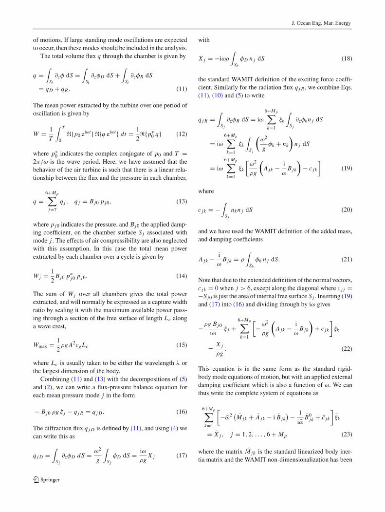
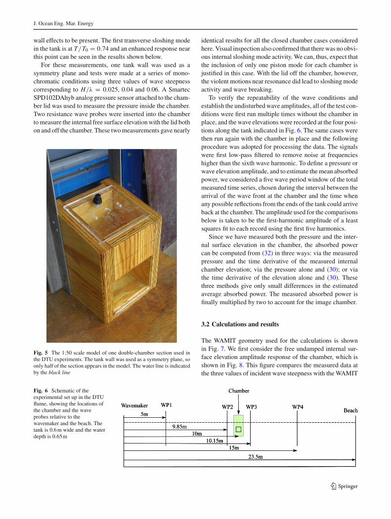
Weprovide here a brief description of the experimental set upand analysis procedure, while more details can be found inDucasse (2014). The physical model used in the experimentsis shown in Fig. 5 and a schematic of the flume is shown inin Fig. 6. The full-scale internal chamber dimensions are 6mby 5m by 7.5m in the x , y and z-directions, respectively, andthe model is at a scale of 1:50. These chamber dimensionsgive an undamped natural period of 5.9 s which is tuned tobe close to a typical value for the conditions in the DanishNorth Sea near the northwest coast of Jylland. The flumeusedhere measures 25m by 0.6m, and the water depth was set to0.65m. The width of the model is 0.1m, so there are only sixchamber widths across the flume, and we can expect some
123
J. Ocean Eng. Mar. Energy
wall effects to be present. The first transverse sloshing modein the tank is at T/T0 = 0.74 and an enhanced response nearthis point can be seen in the results shown below.
For these measurements, one tank wall was used as asymmetry plane and tests were made at a series of mono-chromatic conditions using three values of wave steepnesscorresponding to H/λ = 0.025, 0.04 and 0.06. A SmartecSPD102DAhyb analog pressure sensor attached to the cham-ber lid was used to measure the pressure inside the chamber.Two resistance wave probes were inserted into the chambertomeasure the internal free surface elevationwith the lid bothon and off the chamber. These twomeasurements gave nearly
Fig. 5 The 1:50 scale model of one double-chamber section used inthe DTU experiments. The tank wall was used as a symmetry plane, soonly half of the section appears in the model. The water line is indicatedby the black line
identical results for all the closed chamber cases consideredhere. Visual inspection also confirmed that therewas no obvi-ous internal sloshing mode activity. We can, thus, expect thatthe inclusion of only one piston mode for each chamber isjustified in this case. With the lid off the chamber, however,the violent motions near resonance did lead to sloshingmodeactivity and wave breaking.
To verify the repeatability of the wave conditions andestablish the undisturbedwave amplitudes, all of the test con-ditions were first run multiple times without the chamber inplace, and the wave elevations were recorded at the four posi-tions along the tank indicated in Fig. 6. The same cases werethen run again with the chamber in place and the followingprocedure was adopted for processing the data. The signalswere first low-pass filtered to remove noise at frequencieshigher than the sixth wave harmonic. To define a pressure orwave elevation amplitude, and to estimate themean absorbedpower, we considered a five wave period window of the totalmeasured time series, chosen during the interval between thearrival of the wave front at the chamber and the time whenany possible reflections from the ends of the tank could arriveback at the chamber. The amplitude used for the comparisonsbelow is taken to be the first-harmonic amplitude of a leastsquares fit to each record using the first five harmonics.
Since we have measured both the pressure and the inter-nal surface elevation in the chamber, the absorbed powercan be computed from (32) in three ways: via the measuredpressure and the time derivative of the measured internalchamber elevation; via the pressure alone and (30); or viathe time derivative of the elevation alone and (30). Thesethree methods give only small differences in the estimatedaverage absorbed power. The measured absorbed power isfinally multiplied by two to account for the image chamber.
3.2 Calculations and results
The WAMIT geometry used for the calculations is shownin Fig. 7. We first consider the free undamped internal sur-face elevation amplitude response of the chamber, which isshown in Fig. 8. This figure compares the measured data atthe three values of incident wave steepness with the WAMIT
Fig. 6 Schematic of theexperimental set up in the DTUflume, showing the locations ofthe chamber and the waveprobes relative to thewavemaker and the beach. Thetank is 0.6m wide and the waterdepth is 0.65m
123

J. Ocean Eng. Mar. Energy
X Y
Z
Fig. 7 The submerged geometry of the double-chamber section usedfor theWAMIT calculations. The green (bright) grid shows the internalpressure surface Si , while the olive (dull) grid shows the solid bodysurface S0. Geometry created using the MultiSurf software from Aero-Hydro (2014) (color figure online)
0.4 0.6 0.8 1 1.2 1.4 1.6 1.80
1
2
3
4
5
6
7
8
9
T/T0
| ζ i|/A
ComputedMeasured, H/λ = 0.025Measured, H/λ = 0.04Measured, H/λ = 0.06
Fig. 8 Free undamped internal surface elevation amplitude responseof the chamber plotted vs wave period
calculations. Near resonance, the internal chamber motionsbecome large enough to splash over the top of the chamberand dip below the submerged entrance, leading to stronglynonlinear effects which are, of course, not captured by thecalculations. Away from resonance, however, the agreementcan be seen to be excellent.
The response amplitude for the internal pressure in thechamber with the lid attached is shown in Fig. 9. The calcu-lations here aremadeusing the values of equivalent linearizedPTO damping coefficient shown in Fig. 3. Here, we can seethat the pressures are somewhat over predicted near reso-
0.4 0.6 0.8 1 1.2 1.4 1.6 1.80
0.1
0.2
0.3
0.4
0.5
0.6
0.7
T/T0
|p 0|/ρ
gA
H/λ=.025H/λ=.025. Exp.H/λ=.04H/λ=.04. Exp.H/λ=.06H/λ=.06. Exp.Optimal
Fig. 9 The pressure amplitudes inside the chamber normalized by theincident wave amplitude A
0.4 0.6 0.8 1 1.2 1.4 1.6 1.80
0.5
1
1.5
2
2.5
3
T/T0
Ww.r.t.
L
H/λ=.025H/λ=.025. Exp.H/λ=.04H/λ=.04. Exp.H/λ=.06H/λ=.06. Exp.(B0)opt
Fig. 10 The capture width ratio based on the length of the structure,L = 7.5m, using the PTO damping coefficients shown in Fig. 3
nance, and slightly under predicted in longer waves, but thegeneral behavior and the trends with increasing wave steep-ness are well predicted. The total absorbed power is shownin Fig. 10 in the form of the capture width ratio based on thetotal length of the chamber in the x-direction, L = 7.5m.The comparison here can be seen to follow the internal pres-sure closely, as would be expected. The optimum absorptionpredicted by using (27) as the damping coefficient is alsoshown for reference, and we can see that the theory predictssignificant improvement in the near vicinity of the resonantperiod. In all of these calculations, the finite tank width hasbeen partially accounted for by including one tank wall in theWAMIT analysis. More images of the chamber could also beadded to more fully account for the second wall, but this isleft for future work.
123

J. Ocean Eng. Mar. Energy
Fig. 11 Photo of the scale model ready for testing. A removable bowsection is fitted in this picture, but results are presented here onlywithoutthe bow
4 The response of the full model
We now consider the full 40 chamber model.
4.1 Experiments
The experiments on the full model were carried out atthe Hydraulic and Maritime Research Center (HMRC) atUniversity College Cork, Ireland in 2013. We describe theexperiment briefly here while more details can be found inNielsen (2013) and Pors and Simonsen (2013). A picture ofthe 1:50 scale model is shown in Fig. 11 and a schematicof the experimental set up is shown in Fig. 12. The basinmeasures 25m by 18.5m with a water depth of 1m. It has40 hinged-flap, dry-backed, wave paddles for wave genera-tion, and a 5m long Enkamat beach for wave absorption atthe far end. The model used in these experiments measures3m long by 0.345m wide, with a draft of 0.165m, thus wedo not expect the side walls to have any significant effect onthe measurements in this case. A cluster of five wave probeswas placed approximately 2m in front of the centerline of themodel and a horizontal line of nine probes at 1m intervalswas placed 2.25m behind the model (see Fig. 12). The samebasic experimental and analysis procedure was followed forthese tests as the one described above for the single cham-ber tests. In this case, the model was tested in both regularand irregular waves and in both a fixed and a moored condi-tion. The pressure in all 20 chambers along one side of themodel was measured using pressure sensors and the rigid-body motions were measured using an optical system. Theforces in the mooring system, which is indicated by the solidlines in Fig. 12, were also recorded. Tests were done bothwith and without the removable bow section which is shownin Fig. 11.
Fig. 12 Schematic of the experimental set up atHMRC.The solid linesindicate themooring lines and the points indicate the wave gauges. Thewater depth is 1m and themotionswheremeasured by an optical system
In this paper, we will focus on the regular wave tests,without the bow section, in the fixed and the freely floating(slack-moored) conditions. As in the single chamber tests,the regular waves were tested at wave steepness values ofH/λ = 0.025, 0.04 and 0.06. The internal chamber surfaceelevations were not measured in these tests, so the absorbedpower has been computed from the pressure measurements,together with the pressure–flux relation in (30).
4.2 Fixed model calculations and results
Figure 13 shows the high-order patch boundaries of theWAMIT geometry used for the calculations. This model wasalso created using the MultiSurf software. For the numer-ical solution in this case there are 20 degrees of freedom,one for each pair of chambers. To estimate the equivalentlinearized damping coefficients for each chamber, the pro-cedure described above is applied to iteratively find a set ofcoefficients and responses that satisfy (35). However, herean additional constraint has been added to limit the inter-nal chamber free surface motion amplitude to 2.5m (at fullscale), i.e. the distance from the mean free surface to thetop of the submerged chamber opening. From the assumedrelation between pressure and flux in the chamber (13), thiscondition can be written
ζ j = −B j0
iω|c j j | ξ j → |ξ j | ≤ 2.5
A
ω|c j j |B j0
. (36)
123

J. Ocean Eng. Mar. Energy
X
Y
Z
Fig. 13 The patch boundaries of the submerged geometry for the full40 chamber numericalmodel. The green (bright) patches show the inter-nal pressure surfaces of each chamber
The estimation of the optimal damping coefficients isnow a non-linear optimization problem which has beensolved using the Matlab constrained minimization routinefmincon based on the total absorbed power by all cham-bers with the above mentioned constraint on the maximumresponse amplitude.
Figure 14 shows the resultant damping coefficients andthe pressure response in Chamber number 1, which is at thebow of the structure. Note that since the normalization lengthin this case is twenty times larger than that used for the singlechamber case, themagnitude of B0 ismuch smaller here, eventhough B0 itself is of same order of magnitude in both cases.The same data are shown in Figs. 15 and 16 for chambernumber 10 just forward of themidships section, and chambernumber 20 at the stern of themodel. Experimental data for thefixed model is only available for the H/λ = 0.025 case andthis is also plotted. The agreement between theory and mea-surements is reasonably good, though the calculations tendto generally over-predict the pressures. The numerically opti-mizedvalues are also plotted, andwecan see that the behavior
Fig. 14 Bow chamber: theequivalent linearized dampingcoefficient (left) and thepressure response (right) for thefixed model
0.5 1 1.5 2 2.50
0.02
0.04
0.06
0.08
0.1
0.12
0.14
0.16
0.18
0.2
T/T0
Bj0
H/λ = .025H/λ = .04H/λ = .06Optimal
0.5 1 1.5 2 2.50
0.1
0.2
0.3
0.4
0.5
0.6
0.7
0.8
0.9
1
T/T0
|p 0| /ρ
gA
H/λ = .025H/λ = .025, Exp.H/λ = .04H/λ = .06Optimal
Fig. 15 Midships chamber: theequivalent linearized dampingcoefficient (left) and thepressure response (right) for thefixed model
0.5 1 1.5 2 2.50
0.02
0.04
0.06
0.08
0.1
0.12
0.14
0.16
0.18
0.2
T/T0
Bj0
H/λ = .025H/λ = .04H/λ = .06Optimal
0.5 1 1.5 2 2.50
0.1
0.2
0.3
0.4
0.5
0.6
0.7
0.8
0.9
1
T/T0
| p 0|/ρ
gA
H/λ = .025H/λ = .025, Exp.H/λ = .04H/λ = .06Optimal
123

J. Ocean Eng. Mar. Energy
Fig. 16 Stern chamber: theequivalent linearized dampingcoefficient (left) and thepressure response (right) for thefixed model
0.5 1 1.5 2 2.50
0.02
0.04
0.06
0.08
0.1
0.12
0.14
0.16
0.18
0.2
T/T0
Bj0
H/λ = .025H/λ = .04H/λ = .06Optimal
0.5 1 1.5 2 2.50
0.1
0.2
0.3
0.4
0.5
0.6
0.7
0.8
0.9
1
T/T0
| p 0|/ρ
gA
H/λ = .025H/λ = .025, Exp.H/λ = .04H/λ = .06Optimal
0.8 1 1.2 1.4 1.6 1.8 2 2.20
0.1
0.2
0.3
0.4
0.5
0.6
0.7
0.8
0.9
1
T/T0
Ww.r.t.
L
H/λ = .025H/λ = .025, Exp.H/λ = .04H/λ = .06Optimal
Fig. 17 The capture width ratio of the fixed 40 chamber model withrespect to L = 150m
of the damping coefficients and the pressure responses arequalitatively similar to that of the single chamber, though theamplitudes tend to decrease as we move from bow to stern.
Figure 17 shows the absorbed power as a capture widthratio normalized by the total length of the device L = 150m.The general over-prediction of the chamber pressures leads,as would be expected, to a general over-prediction of thedevice absorption width for wave periods above the resonantperiod. As for the single chamber case, substantial improve-ment in absorption is predicted near the resonant periodwhenan optimal damping coefficient is applied. Unfortunatelythere is a gap in the experimental data near the resonanceperiod, but new experiments are in progress to fill in thisregion.
4.3 Freely floating model calculations and results
In the freely floating case, we add the six rigid-body modesto the 20 pressure-surface modes to get 26 degrees of free-
dom. The rigid-body motions of the structure also induceflux in the chambers, so the pressure response ξ j is now thecombined result of the rigid-body motions and the internalsurface motion. The internal surface elevation ζ j , measuredrelative to the mean water line of chamber j , is thus given by
q j = |c j j | iωζ j , ζ j = ζ j0 − ξ3 + x j ξ5 + y j ξ4 (37)
where ζ j0 = ζ j0/A is the non-dimensional surface elevationamplitude relative to the still water level, and ξ3, ξ4, ξ5 repre-sent the heave, roll and pitch motion amplitudes respectively.If the non-dimensional x and y-coordinates of the center ofchamber j are given by x j , y j , then the hydrostatic couplingbetween the pressure response and the heave, pitch and rollmodes is given by
c3k = Sk0; c4k = yk Sk0; c5k = −xk Sk0, for 6 < k <= Mp
(38)
This interaction is symmetric, so these coefficients are alsoreflected across the diagonal of the c jk matrix. With thesemodifications, the solution proceeds as described above inthe fixed body case.
The results for the damping coefficients and pressuresin the bow, mid-section and stern chambers are shown inFigs. 18, 19 and 20. The experimental results for the mea-sured pressures are also shown. The agreement betweencalculations and measurements is satisfactory with a generalover-prediction near the resonant period and some under-prediction in long waves. It is clear that the motions havea significant effect on the local pressures in the chamberscompared to the fixed body case.
Figure 21 shows the absorbed power as a capture widthratio normalized by the total length of device L = 150m.The agreement here is perhaps slightly better than in thefixed model case. Interestingly, both calculations and exper-
123

J. Ocean Eng. Mar. Energy
Fig. 18 Bow chamber: theequivalent linearized dampingcoefficient (left) and thepressure response (right) for thefreely floating model
1 1.5 2 2.50
0.02
0.04
0.06
0.08
0.1
0.12
0.14
0.16
0.18
0.2
T/T0
Bj0
H/λ = .025H/λ = .04H/λ = .06Optimal
1 1.5 2 2.50
0.5
1
1.5
T/T0
| p 0|/ρ
gA
H/λ = .025H/λ = .025, Exp.H/λ = .04H/λ = .04, Exp.H/λ = .06H/λ = .06, Exp.Optimal
Fig. 19 Midships chamber: theequivalent linearized dampingcoefficient (left) and thepressure response (right) for thefreely floating model
1 1.5 2 2.50
0.02
0.04
0.06
0.08
0.1
0.12
0.14
0.16
0.18
0.2
T/T0
Bj0
H/λ = .025H/λ = .04H/λ = .06Optimal
1 1.5 2 2.50
0.5
1
1.5
T/T0
|p 0|/ρ
gA
H/λ = .025H/λ = .025, Exp.H/λ = .04H/λ = .04, Exp.H/λ = .06H/λ = .06, Exp.Optimal
Fig. 20 Stern chamber: theequivalent linearized dampingcoefficient (left) and thepressure response (right) for thefreely floating model
1 1.5 2 2.50
0.02
0.04
0.06
0.08
0.1
0.12
0.14
0.16
0.18
0.2
T/T0
Bj0
H/λ = .025H/λ = .04H/λ = .06Optimal
1 1.5 2 2.50
0.5
1
1.5
T/T0
|p 0|/ ρ
gA
H/λ = .025H/λ = .025, Exp.H/λ = .04H/λ = .04, Exp.H/λ = .06H/λ = .06, Exp.Optimal
123

J. Ocean Eng. Mar. Energy
iments predict that the motions have a positive effect onthe absorption near the resonant frequency, but a negativeeffect in long waves. The optimized damping coefficientspredict a similar improvement in absorption to that whichwas found in the fixed model case. The left hand plot inFig. 22 shows the same calculations normalized with respectto the incident wavelength λ for reference. The right handplot in Fig. 22 shows the predicted mean absorbed powerin megawatts at full scale as a function of wave period forthe three considered wave steepness values. This gives anindication of the real potential of such a device and alsoillustrates the large variability in absorbed power inherentto wave energy. As discussed above, a maximum of about80% of this absorbed power will be converted into electricalpower depending on the conditions and the actual air turbinesused. It could also be attractive to consider using valves to
0.6 0.8 1 1.2 1.4 1.6 1.8 2 2.2 2.4 2.60
0.1
0.2
0.3
0.4
0.5
0.6
0.7
0.8
0.9
1
T/T0
Ww.r.t.
L
H/λ = .025H/λ = .025, Exp.H/λ = .04H/λ = .04, Exp.H/λ = .06H/λ = .06, Exp.Optimal
Fig. 21 The capture width ratio of the moored 40 chamber model withrespect to L = 150m
0 0.2 0.4 0.6 0.8 1 1.2 1.4 1.60
0.1
0.2
0.3
0.4
0.5
0.6
0.7
0.8
0.9
1
λ/L
| ξ 1|/A
H/λ = .025H/λ = .025, Exp.H/λ = .04H/λ = .04, Exp.H/λ = .06H/λ = .06, Exp.Optimal
Fig. 23 The surge motion response of the full 40 chamber model
0 0.2 0.4 0.6 0.8 1 1.2 1.4 1.60
0.1
0.2
0.3
0.4
0.5
0.6
0.7
0.8
0.9
1
λ/L
|ξ 3|/A
H/λ = .025H/λ = .025, Exp.H/λ = .04H/λ = .04, Exp.H/λ = .06H/λ = .06, Exp.Optimal
Fig. 24 The heave motion response of the full 40 chamber model
Fig. 22 The capture width ratioof the freely floating 40 chambermodel with respect to thewavelength λ (left), and thepredicted full-scale powerabsorption in megawatts (right)
1 1.5 2 2.50
0.2
0.4
0.6
0.8
1
1.2
1.4
1.6
1.8
2
T/T0
Ww.r.t.
λ
H/λ = .025H/λ = .04H/λ = .06Optimal
4 6 8 10 12 14 16 180
2
4
6
8
10
12
14
16
18
20
T [s]
W[M
W]
H/λ = .025H/λ = .025, Exp.H/λ = .04H/λ = .04, Exp.H/λ = .06H/λ = .06, Exp.
123

J. Ocean Eng. Mar. Energy
0 0.2 0.4 0.6 0.8 1 1.2 1.4 1.60
0.1
0.2
0.3
0.4
0.5
0.6
0.7
0.8
0.9
1
λ/L
|ξ 5|/k
A
H/λ = .025H/λ = .025, Exp.H/λ = .04H/λ = .04, Exp.H/λ = .06H/λ = .06, Exp.Optimal
Fig. 25 The pitch motion response of the full 40 chamber model
connect all the chambers to a central channel to drive oneunidirectional flow through a larger and more efficient tur-bine.
Figures 23, 24 and 25 show the rigid-body motionresponse of the structure in the surge, heave and pitchmodes, respectively. These results are normalized by thewave amplitude A and the wave slope k A for translationaland rotational modes, respectively, and are plotted versusthe relative incident wavelength. Here, we can see a goodagreement between the calculations and the measurements,especially in the target wave period region where the rigid-body motions are small. The increased pressures in thechambers near resonance which are predicted by the opti-mized damping coefficients can be seen to introduce anenhanced pitch response there. We note that the mooringsystem introduces a very long natural period to the surgeresponse of the structure, but this period is far beyond thewind-wave spectrum which we focus on here. We note alsothat the vertical center of gravity and the pitch radius ofgyration of the ballasted model were used in the calcula-tions.
5 Conclusions
In this paper, we have clarified several subtle details whichare important to getting good performance out of standardfrequency domain, linear potential flow theory for the analy-sis of floating structures which include one or more OWCdegrees of freedom. This has been illustrated by consideringboth a fixed single degree of freedom OWC and an I-beamattenuator OWC device with 26 degrees of freedom. Theagreement between calculations and measurements is gen-erally found to be excellent, though the calculations tendto slightly over-predict the internal chamber pressures andtherefore the absorbed power near resonance, but under-
predict these quantities in long waves in the freely floatingcondition.
Future work will focus on weakly non-linear calculationsin the time domain which will allow for a better model of theair turbine and inclusion of some viscous and air compress-ibility effects. Possible improvements to the design whichare currently under investigation include: replacing the sim-ple chamber with a U-OWC chamber; replacing the OWCwith a simple mechanical oscillator; and introducing a valvesystem to rectify the air flow from all chambers to a centralplenum and one large unidirectional turbine. Survivabilitytests, structural calculations and detailed mooring systemdesign are also in progress to get an accurate estimate ofthe final cost of energy for such a system.
Acknowledgments The authors would like to thank Pablo Guillenfor generating the 40 chamber geometry, and Frederik Pors Jakob-sen and Morten Simonsen for building the models and carryingout the experimental measurements on the 40 chamber model. TheHMRC experiments received support from MARINET, a EuropeanCommunity—Research Infrastructure Action under the FP7 “Capac-ities” Specific Programme.
References
AeroHydro (2014) Relational 3D modeling for marine and industrialdesign. http://aerohydro.com. Accessed 1 Jan 2014
Barstow S, Mørk G, Mollison D, Cruz J (2008) The wave energyresource. In: Cruz J (ed) Ocean wave energy, Current status andfuture perspectives. Springer, Berlin
Boccotti P (2007) Comparison besteen a U-OWC and a conventionalOWC. Ocean Eng 34:799–805
Boccotti P, Filianoti P, Fiamma V, Arena F (2007) Caisson breakwatersembodying an OWC with a small opening. Part II: a small-scalefield experiment. Ocean Eng 34:820–841
Boccotti P (2012) Design of breakwaters for conversion of wave energyinto electrical energy. Ocean Eng 51:106–118
Boccotti P (2015)Wavemechanics andwave loads onmarine structures.Butterworth-Heinemann, Amsterdam
CarbonTrust (2005) Oscillating water column wave energy converterevaluation report. http://www.carbontrust.com/media/173555/owc-report.pdf. Accessed 1 Jan 2014
Cruz J (2008) Ocean wave energy, Current status and future perspec-tives. Springer, Berlin
Drew B, Plummer AR, Sahinkaya M (2009) A review of wave energyconverter technology. Proc Inst Mech Eng Part A-J Power Energy223:887–902
DucasseD (2014) A theoretical and experimental study of an oscillatingwater column attenuator. Master’s thesis, Technical University ofDenmark, Lyngby
Evans DV (1982) Wave-power absoption by systems of oscillating sur-face pressure distributions. J Fluid Mech 114:481–499
Falcão AFO (2010) Wave energy utilization: a review of the technolo-gies. Renew Sustain Energy Rev 14:899–918
FalcãoAFO,Gato LMC,Nunes EPAS (2013)A novel self-rectifying airturbine for use in wave energy converters. Renew Energy 50:289–298
Falcão AFO, Henriques JCC (2014) Model-prototype similarity ofoscillating-water-column wave energy converters. Int J MarEnergy 6:18–34
123

J. Ocean Eng. Mar. Energy
Falnes J (2002) Ocean waves and oscillating systems. Cambridge Uni-versity Press, Cambridge
Heath T (2012) A review of oscillating water columns. Phil Trans RSoc Lond A 370:235–245
IEA (2014) OES—ocean energy systems, an international energyagency technology initiative. http://www.ocean-energy-systems.org. Accessed 1 Jan 2014
Ishii S, Miyazaki T, Masuda Y, Kai G (1982) Reports and future plansfor the kaimei project. In: Proc 2nd international symposium onwave energy utilization, Trondheim, Norway
Jacobsen P (2011) Mapping and assessment of the United States oceanwave energy resource. In: Technical report 1024637. ElectricPower Research Institute, Palo Alto
Lee C-H, Newman JN, Nielsen FG (1996) Wave interactions with anoscillating water column. In: 6th intl. offshore and polar engineer-ing conference, Los Angeles, USA
Lee C-H, Nielsen FG (1996) Analysis of oscillating water columndevice using a panel method. In: 11th intl wrkshp water wavesand floating bodies, Hamburg, Germany. http://www.iwwwfb.org.Accessed 1 Jan 2014
López I, Andreu J, Ceballos S, Martinez de Alegria I, Kortabarria I(2013) Review of wave energy technologies and the necessarypower-equipment. Renew Sustain Energy Rev 27:413–434
Masuda Y (1979) Experimental full scale result of wave power machineKaimei in 1978. In: Proc. 1st inter symponwave energy utilization,Gothenburg, Sweden
McCormick M (2007) Ocean wave energy conversion. Dover, Mineola
Moody GW (1980) The NEL oscillating water column: recent develop-ments. In: First symposium on wave energy utilization, Oct 1979.Chalmers University of Technology, Gothenburg, pp 283–296
Newman JN, Lee C-H (2014) WAMIT; a radiation-diffraction panelprogram for wave-body interactions. http://www.wamit.com.Accessed 1 Jan 2014
Nielsen K (2013) Final report: KNSWING attenuator developmentphase I. Technical report, FP7-MARINET, marine renewablesinfrastructure network. http://www.fp7-marinet.eu/. Accessed 1Jan 2014
OEE (2014) Ocean energy Europe, a trade association for Oceanrenewables. http://www.oceanenergy-europe.eu/index.php/en/.Accessed 1 Jan 2014
Oyster (2014) Aquamarine power. http://aquamarinepower.com/.Accessed 1 Jan 2014
Pelamis (2014) Pelamis wave power. http://www.pelamiswave.com/.Accessed 1 Jan 2014
Pors F, Simonsen M (2013) A theoretical and experimental study of anoscillating water column attenuator. BS thesis, Technical Univer-sity of Denmark, Lyngby
SIOcean (2012) Ocean energy: state of the art. Strategic initiative forOcean energy. http://si-ocean.eu. Accessed 1 Jan 2014
WAVENERGY.IT (2014) WAVENERGY.IT S.r.l. http://wavenergy.it/.Accessed 1 Jan 2014
Wavestar (2014) Wavestar energy. http://wavestarenergy.com/.Accessed 1 Jan 2014
123